ESTIMATION OF ANNUAL AVERAGE DAILY TRAFFIC ON LOCAL …

University of Kentucky University of Kentucky

UKnowledge UKnowledge

Theses and Dissertations--Civil Engineering Civil Engineering

2016

ESTIMATION OF ANNUAL AVERAGE DAILY TRAFFIC ON LOCAL ESTIMATION OF ANNUAL AVERAGE DAILY TRAFFIC ON LOCAL

ROADS IN KENTUCKY ROADS IN KENTUCKY

William Nicholas Staats University of Kentucky, [email protected] Digital Object Identifier: http://dx.doi.org/10.13023/ETD.2016.066

Right click to open a feedback form in a new tab to let us know how this document benefits you. Right click to open a feedback form in a new tab to let us know how this document benefits you.

Recommended Citation Recommended Citation Staats, William Nicholas, "ESTIMATION OF ANNUAL AVERAGE DAILY TRAFFIC ON LOCAL ROADS IN KENTUCKY" (2016). Theses and Dissertations--Civil Engineering. 36. https://uknowledge.uky.edu/ce_etds/36

This Master's Thesis is brought to you for free and open access by the Civil Engineering at UKnowledge. It has been accepted for inclusion in Theses and Dissertations--Civil Engineering by an authorized administrator of UKnowledge. For more information, please contact [email protected].

http://uknowledge.uky.edu/

http://uknowledge.uky.edu/

https://uknowledge.uky.edu/

https://uknowledge.uky.edu/ce_etds

https://uknowledge.uky.edu/ce

https://uky.az1.qualtrics.com/jfe/form/SV_9mq8fx2GnONRfz7

mailto:[email protected]

STUDENT AGREEMENT: STUDENT AGREEMENT:

I represent that my thesis or dissertation and abstract are my original work. Proper attribution

has been given to all outside sources. I understand that I am solely responsible for obtaining

any needed copyright permissions. I have obtained needed written permission statement(s)

from the owner(s) of each third-party copyrighted matter to be included in my work, allowing

electronic distribution (if such use is not permitted by the fair use doctrine) which will be

submitted to UKnowledge as Additional File.

I hereby grant to The University of Kentucky and its agents the irrevocable, non-exclusive, and

royalty-free license to archive and make accessible my work in whole or in part in all forms of

media, now or hereafter known. I agree that the document mentioned above may be made

available immediately for worldwide access unless an embargo applies.

I retain all other ownership rights to the copyright of my work. I also retain the right to use in

future works (such as articles or books) all or part of my work. I understand that I am free to

register the copyright to my work.

REVIEW, APPROVAL AND ACCEPTANCE REVIEW, APPROVAL AND ACCEPTANCE

The document mentioned above has been reviewed and accepted by the student’s advisor, on

behalf of the advisory committee, and by the Director of Graduate Studies (DGS), on behalf of

the program; we verify that this is the final, approved version of the student’s thesis including all

changes required by the advisory committee. The undersigned agree to abide by the statements

above.

William Nicholas Staats, Student

Dr. Reginald R. Souleyrette, Major Professor

Dr. Yi-Tin Wang, Director of Graduate Studies

ESTIMATION OF ANNUAL AVERAGE DAILY

TRAFFIC ON LOCAL ROADS IN KENTUCKY

___________________________________

THESIS

___________________________________

A thesis submitted in partial fulfillment of the

requirements for the degree of Master of Science in Civil Engineering

in the College of Engineering at the University of Kentucky

By

William Nicholas Staats

Lexington, Kentucky

Director: Dr. Reginald R. Souleyrette, Professor of Civil Engineering

2016

Copyright © William Nicholas Staats 2016

ABSTRACT OF THESIS



Annual average daily traffic (AADT) is used to estimate intersection performance across

Kentucky. The Kentucky Transportation Cabinet (KYTC) currently collects AADTs for

state maintained roads, but lacks this information on local roads. A method is needed to

estimate local road AADTs in a cost-effective and reasonable manner. A literature review

was conducted on AADT models and found no models suitable to Kentucky. Therefore an

AADT model using non-linear regression was developed for local roads in Kentucky

This model divided the state into three regions utilizing Kentucky’s highway districts. This

partitioning accounted for geographic and socioeconomic variability across the state. Each

regional model relied upon three independent variables: probe count, residential vehicle

registration, and curve rating. HERE proprietary probe counts provide tracking visibility

on a select portion of vehicles moving across Kentucky highways. Residential vehicle

registrations were used to estimate trip generation information. Finally, the curve rating

partially indicates accessibility.

The models were adjusted to KYTC daily vehicle miles traveled (DVMT) county control

totals for local roads. Sensitivity analysis was conducted to examine the impact of model

errors for use in intersection safety analysis. Results indicate that the estimates generated

can be effectively used for safety assessment and countermeasure prioritization.

Key Words: Local Road, AADT, Estimating, Modeling



By

William Nicholas Staats

Reginald R. Souleyrette

Director of Thesis

Yi-Tin Wang

Director of Graduate Studies

April 20, 2016

Date

iii

ACKNOWLEDGEMENTS

The following thesis benefited from the insights, direction, and support of several people.

First I would like to express the deepest gratitude to my Thesis Chair, Dr. Reginald R.

Souleyrette, for providing me with educational guidance, technical assistance, and

financial support throughout my graduate school career despite his overwhelming schedule

as the Chair of the Civil Engineering Department. Not only did Dr. Souleyrette guide me

through graduate school, he influenced me during my undergraduate career as well. He has

been a role model for me since I was a freshman when I first met with him for academic

advising. He serves as an excellent example of what it means to be a good professional, a

good engineer, and an all-around good person.

Next I wish to thank my entire Thesis Committee including Dr. Reginald R. Souleyrette,

Dr. Mei Chen, and Dr. Kamyar Mahboub, for encouraging me to convert my Master’s final

project into a thesis.

I would also like to thank my co-workers and fellow graduate students, Eric Green and

Brian Howell, for contributing ideas, suggestions, and editorial assistance toward my

thesis. Eric was always available to bounce ideas off of and Brian assisted with fine-tuning

the writing of my thesis.

Finally, I would like to thank my mother for all the support she provides me every day, and

my brother who went and earned himself a graduate degree, forcing me to earn one myself

so he couldn’t say he was more educated.

iv

TABLE OF CONTENTS

ACKNOWLEDGEMENTS ................................................................................................ iii

LIST OF TABLES .............................................................................................................. vi

LIST OF FIGURES ........................................................................................................... vii

CHAPTER 1: BACKGROUND ......................................................................................... 1

1.1 INTRODUCTION .................................................................................................... 1

1.2 PROBLEM STATEMENT ....................................................................................... 1

1.3 OBJECTIVES ........................................................................................................... 2

CHAPTER 2: LITERATURE REVIEW ............................................................................ 3

2.1 AADT METHODOLOGIES .................................................................................... 3

2.1.1 ORDINARY LINEAR REGRESSION MODEL .............................................. 4

2.1.2 GEOGRAPHICALLY WEIGHTED REGRESSION MODEL ........................ 6

2.1.3 KRIGING INTERPOLATION MODEL ........................................................... 7

2.1.4 ARTIFICIAL NEURAL NETWORK ............................................................... 8

2.1.5 TRAVEL DEMAND MODELING ................................................................... 8

2.1.6 ORIGIN-DESTINATION (OD) CENTRALITY-BASED METHOD ............. 9

2.1.7 FLORIDA TURNPIKE MODEL .................................................................... 10

2.2 DISCUSSION AND RECOMMENDATION ........................................................ 10

CHAPTER 3: AADT MODEL ......................................................................................... 11

3.1 MODEL DEVELOPMENT .................................................................................... 11

3.2 DATA COLLECTION ........................................................................................... 12

3.2.1 SHORT DURATION TRAFFIC COUNTS .................................................... 13

3.2.2 KYTC AADT DATA ...................................................................................... 13

3.2.3 AVIS DATA .................................................................................................... 14

3.2.4 HERE DATA ................................................................................................... 14

3.3 KENTUCKY AADT MODEL ............................................................................... 15

3.3.1 AVIS-HERE NON-LINEAR REGRESSION MODEL .................................. 15

3.3.2 RURAL MODEL DEVELOPMENT .............................................................. 18

3.3.3 RURAL MODEL RESULTS .......................................................................... 23

3.3.4 URBAN MODEL DEVELOPMENT .............................................................. 32

3.3.5 URBAN MODEL RESULTS .......................................................................... 33

CHAPTER 4: SENSITIVITY ANALYSIS ...................................................................... 36

v

4.1 SENSITIVITY ANALYSIS ................................................................................... 36

4.1.1 KYTC CRASHES AND ASSOCIATED COSTS ........................................... 36

4.1.2 SENSITIVITY ANALYSIS METHODOLOGY ............................................ 37

4.1.3 RURAL MODEL SENSITIVITY ANALYSIS .............................................. 38

4.1.4 URBAN MODEL SENSITIVITY ANALYSIS .............................................. 41

CHAPTER 5: CONCLUSION ......................................................................................... 44

5.1 FINDINGS .............................................................................................................. 44

5.2 RECOMMENDATIONS ........................................................................................ 44

APPENDIX A: BROWARD COUNTY MODEL ........................................................... 46

APPENDIX B: BROWARD COUNTY WITH PVA MODEL ....................................... 53

APPENDIX C: ROOFTOP MODEL................................................................................ 55

APPENDIX D: 911 MODEL............................................................................................ 57

APPENDIX E: AVIS-HERE MODEL, ORDINARY LINEAR REGRESSION ........... 59

REFERENCES ................................................................................................................. 61

VITA ................................................................................................................................. 63

vi

LIST OF TABLES

Table 1: AADT Methodologies .......................................................................................... 3

Table 2: AVIS Data .......................................................................................................... 14

Table 3: Rural Regional Model Coefficients .................................................................... 23

Table 4: Rural Regional Model Errors.............................................................................. 24

Table 5: Rural Regional Model Errors with DVMT Adjustment Factor .......................... 29

Table 6: Urban Regional Model Coefficients ................................................................... 33

Table 7: Urban Regional Models Errors ........................................................................... 33

Table 8: Urban DVMT Control Total Data ...................................................................... 34

Table 9: Errors from Urban Regional Models after DVMT Adjustment ........................ 35

Table 10: FHWA Crash Cost Estimates by Crash Severity .............................................. 37

vii

LIST OF FIGURES

Figure A: KYTC Traffic Counts, Franklin Co.................................................................. 13

Figure B: AVIS Residential and Commercial Properties, Meade County........................ 16

Figure C: ArcMap Geocoding Inputs ............................................................................... 17

Figure D: KYTC Roadway Segments............................................................................... 19

Figure E: Modified Roadway Segments ........................................................................... 20

Figure F: HERE Probe Data Segments ............................................................................. 21

Figure G: Geographical Distribution of Errors ................................................................. 25

Figure H: Validation Errors in Three Regional Models ................................................... 26

Figure I: West Regional Model, Known vs. Model AADT .............................................. 26

Figure J: North-Central Regional Model, Known vs. Model AADT ............................... 27

Figure K: East Regional Model, Known vs. Model AADT ............................................. 27

Figure L: VMT Adjustment Ratio by County................................................................... 28

Figure M: Validation Errors in Three Regional Models (w/ Adjustment Factor) ............ 30

Figure N: West Regional Model, Known vs Model AADT (w/ Adjustment) .................. 31

Figure O: North-Central Regional Model, Known vs Model AADT (w/ Adjustment).... 31

Figure P: East Regional Model, Known vs Model AADT (w/ Adjustment) .................... 32

1

CHAPTER 1: BACKGROUND

1.1 INTRODUCTION

Annual average daily traffic (AADT) provide transportation planners and safety engineers

with critical roadway information to estimate performance, but limitations in data

collection have left much of Kentucky’s highway network unevaluated. The Federal

Highway Administration (FHWA) defines AADT as the “total volume of vehicle traffic of

a highway or road for a year divided by 365 days” (1). Transportation planners and policy

decision-makers rely heavily on AADT metrics to assess highway performance and guide

their future planning and funding decisions. For instance, AADT assists in the calculation

of vehicle miles travelled (VMT) which, in turn, establishes the basis for distributing

highway funds related to maintenance and safety. Furthermore, AADT serves as the

framework for estimating other transportation planning factors including crash rate

predictions, vehicle emissions, and forecasting future travel demand. For these reasons,

state department of transportation (DOT) planners and other affected stakeholders often

take great efforts to collect and utilize this data.

Through its Traffic Monitoring System, the Kentucky Transportation Cabinet (KYTC)

collects highway traffic data to develop AADTs on all state-maintained roads and local

roads functionally classified as Collector or above. This generally involves segmenting the

entire roadway system and using Automatic Data Recorders (ADRs) placed in each

segment to collect data for a minimum of 48 hours every three years. Factors are derived

from sites that collect data continuously – Automatic Traffic Recorders (ATRs) – and used

to annualize these short duration counts into AADTs.

Currently, Kentucky has significant gaps in collecting traffic data across its non-state

maintained transportation network. The collection of traffic data to develop AADTs on

non-state roads—also referred to as local roads—is optional for county and city agencies.

Metropolitan Planning Organizations (MPOs) and Area Development Districts (ADDs)

may also collect data. These agencies may also employ the use of ADR equipment to

determine their respective AADT. However, many local agencies struggle in their traffic

data collection efforts due to their limited fiscal resources, labor shortages, and in some

cases, the lack of expertise and/or political will. For these reasons, AADT across many of

these local roads remains unknown. To date, KYTC has obtained AADT for approximately

1,200 miles of local roadways across the entire state. This study will hereafter refer to

KYTC-provided AADT as “known” AADT, subsequently used to develop and validate the

AADT models. This represents only 2 percent of the state’s 52,000 miles of local roadways.

Consequently, approximately 98 percent of the local roadways in Kentucky currently lack

AADT thereby posing planning and funding challenges to highway officials.

1.2 PROBLEM STATEMENT

KYTC and other highway agencies rely heavily on the use of AADT in safety analysis.

This research provides a method of estimating AADTs and supports KYTC’s ability to

plan and prioritize safety mitigations.

2

1.3 OBJECTIVES

This report describes the development of a model to estimate AADT for local roads in

Kentucky. To achieve this objective, the following tasks were completed:

a. Research available AADT transportation models in use or previously developed by

other state DOTs, universities, or other research organizations, and determine

capabilities, requirements, and accuracy of selected models

b. Select an AADT transportation model that can be successfully applied to

Kentucky’s local roadway network

c. Revise and adjust model to fit the data available for Kentucky and produce relevant,

accurate, and precise model outputs

d. Validate and calibrate developed model using known local roadway data

3

CHAPTER 2: LITERATURE REVIEW

2.1 AADT METHODOLOGIES

Various methodologies were investigated that have been used across the United States to

estimate AADTs. Several methodologies were selected based upon a wide range of peer-

reviewed scientific articles published by practitioners and researchers within the

transportation planning community. This comprehensive approach to AADT estimation

provided a rigorous overview of best practices currently being used as well as those

methods which may be best suited to Kentucky’s roadway network. Academic universities

and state DOTs developed the majority of the methods described in this section. In Table

1 below, AADT methodologies, corresponding sources, and facilities of interest are shown.

Table 1: AADT Methodologies

Methodology Source Facilities of Interest

Ordinary Linear regression

Pan (2) All roads in Florida

Shen et al. (3) Off-system roads in Florida

Zhao and Chung (4) County roads in Florida

Lowry and Dixon (5) Streets in an urban area

Mohammad et al. (6) County roads in Indiana

Geographically weighted

regression Zhao and Park (7) County roads

Kriging interpolation

Selby and Kockelman

(8) All roads in Texas

Eom et al. (9) Non-freeway roads in a

county

Shamo et al. (10) Roadways with ATR data

Wang and Kockelman

(11) All roads in Texas

Artificial Neural Network Sharma et al. (12) Rural roads

Travel demand modeling

Wang et al. (13) All roads in Florida

Wang (14) All roads in Florida

Zhong and Hanson (15) Low-class roads

Origin-Destination centrality

based Method Lowry (16) Community roads

Florida Turnpike state model Florida DOT (17, 18) Roads without traffic counts

4

The following sections provide brief descriptions of each methodology. This discussion

includes an outline of the modeling equations, data input requirements, and an examination

of select source models.

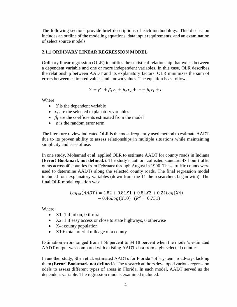
2.1.1 ORDINARY LINEAR REGRESSION MODEL

Ordinary linear regression (OLR) identifies the statistical relationship that exists between

a dependent variable and one or more independent variables. In this case, OLR describes

the relationship between AADT and its explanatory factors. OLR minimizes the sum of

errors between estimated values and known values. The equation is as follows:

𝑌 = 𝛽0 + 𝛽1𝑥1 + 𝛽2𝑥2 + ⋯ + 𝛽𝑖𝑥𝑖 + 𝜀

Where

Y is the dependent variable

𝑥𝑖 are the selected explanatory variables

𝛽𝑖 are the coefficients estimated from the model

𝜀 is the random error term

The literature review indicated OLR is the most frequently used method to estimate AADT

due to its proven ability to assess relationships in multiple situations while maintaining

simplicity and ease of use.

In one study, Mohamad et al. applied OLR to estimate AADT for county roads in Indiana

(Error! Bookmark not defined.). The study’s authors collected standard 48-hour traffic

ounts across 40 counties from February through August in 1996. These traffic counts were

used to determine AADTs along the selected county roads. The final regression model

included four explanatory variables (down from the 11 the researchers began with). The

final OLR model equation was:

𝐿𝑜𝑔10(𝐴𝐴𝐷𝑇) = 4.82 + 0.81𝑋1 + 0.84𝑋2 + 0.24𝐿𝑜𝑔(𝑋4)− 0.46𝐿𝑜𝑔(𝑋10) (𝑅2 = 0.751)

Where

X1: 1 if urban, 0 if rural

X2: 1 if easy access or close to state highways, 0 otherwise

X4: county population

X10: total arterial mileage of a county

Estimation errors ranged from 1.56 percent to 34.18 percent when the model’s estimated

AADT output was compared with existing AADT data from eight selected counties.

In another study, Shen et al. estimated AADTs for Florida “off-system” roadways lacking

them (Error! Bookmark not defined.). The research authors developed various regression

odels to assess different types of areas in Florida. In each model, AADT served as the

dependent variable. The regression models examined included:

5

Statewide model

Rural model

Small-medium urban model

Large metropolitan area model

In particular, this “rural” based model incorporated data from eight counties. The final

regression equation was:

ADT = 4853.49 + 0.12 Pop + 0.26 Labor - 18.93 Lanemile -

0.0032338 Vehicles

Where

Pop is a county’s total population;

Labor is a county’s total labor force;

Lanemile is the total lane miles of county roads in a county;

Vehicles is the number of automobiles registered in a county;

Upon initial examination, this model seemed to show promise for assessing rural roads, a

primary element of Kentucky’s local roadway network. However, the model’s coefficient

of determination, or R-squared, was only 0.25. The R-squared value can be translated as

the percentage of variance in “Y” (or ADT) that is explained by the dependent variables.

This means the model only explained 25 percent of the ADT value using its explanatory

variables. Consequently, the model’s overall usefulness is limited in estimating AADT

values in Kentucky.

Similarly, Zhao and Chung used regression modeling to assess various factors and their

ability to estimate AADTs (Error! Bookmark not defined.). The researchers examined

our unique regression models to estimate AADTs in Broward County, Florida. This yielded

the following regression equations:

Model 1: AADT = -9.520386 + 8.480001 FCLASS + 3.428939 LANE + 0.596752

REACCESS + 2.991573 DIRECTAC + 0.069086 EMPBUFF

Model 2: AADT = -6.15742 + 6.55471 LANE + 0.61433 REACCESS + 7.88344

DIRECTAC – 0.34494 DPOPCNTR


DIRECTAC – 0.10689 DPOPCNTR + 0.00112 POPBUFF


DIRECTAC – 0.10197 DPOPCNTR + 0.00104 POPBUFF +

0.00022820 EMPBUFF

6

Where

FCLASS is functional classification of roadway

LANE is the number of lanes in both directions

REACCESS is the access to regional employment

DIRECTAC is direct access (or connection) to an expressway

EMPBUFF is the number of people employed along a roadway segment

DPOPCNTR is the distance to a population center

POPBUFF is the number of people living along a roadway segment

These regression models produced R-squared values ranging from 0.66 to 0.82, a

significantly higher precision over other regression models. In addition, these models

examined a larger set of variables than regression models developed by other researchers,

thus leading to a more comprehensive approach in determining AADT. For these reasons,

these regression models exhibited the greatest initial promise for inclusion into a Kentucky-

based model, therefore the variables used in these regression models were selected for

further study and analysis.

2.1.2 GEOGRAPHICALLY WEIGHTED REGRESSION MODEL

Geographically weighted regression (GWR) models account for transportation network

spatial variation. Unlike OLR models, GWR generates equations locally for each

observation. For this reason, a GWR model is generally considered more capable in

accurately estimating results than comparable OLR models. The basic equation is as

follows:

𝑌𝑖 = 𝛽0(𝑢𝑖, 𝑣𝑖) + 𝛽1(𝑢𝑖, 𝑣𝑖)𝑥𝑖1 + 𝛽2(𝑢𝑖, 𝑣𝑖)𝑥𝑖2 + ⋯ + 𝛽𝑘(𝑢𝑖, 𝑣𝑖)𝑥𝑖𝑘

+ 𝜀𝑖

Where

𝑌𝑖 is the AADT

𝑖 is the ith observation

𝛽𝑘(𝑢𝑖, 𝑣𝑖) is the coefficient of local model to be estimated

𝑥𝑖𝑘 is the kth variable from ith observation

𝜀𝑖 is the random (model) error

The GWR model examines each observation and then selects those observations found in

close proximity to a selected geospatial area for further consideration. In those instances,

the model estimates the coefficient using a weighted factor which, in turn, relies upon a

weighting function for its calculation. Simply put, locations found closer to the roadway of

interest will receive higher weighted values on their explanatory factors. This is because

those nearby areas are considered to have proportionately larger impacts on the travel

demands of the geographical area of interest.

Zhao and Park applied this concept to develop two distinct GWR models used in estimating

AADTs and utilized data from Zhao and Chung’s OLR model (4). While more difficult to

7

implement, both GWR models showed improvements in performance over the previous

OLR model, with higher R-squared values and smaller estimation errors.

2.1.3 KRIGING INTERPOLATION MODEL

The Kriging model uses spatial interpolation to estimate unknown values at locations or

points based on known values at nearby locations or points (19). This method assumes that

observations are spatially correlated. It subsequently generates a function based on this

spatial relationship. In this manner, Kriging generates a prediction surface from existing

points to estimate values of a parameter at unknown locations. The model equation is as

follows:

�̂�(𝑆0) = ∑ 𝜆𝑖

𝑛

𝑖=1

𝑍(𝑆𝑖)

Where

�̂�(𝑆0) is the value to be estimated

𝑆0 is the location to be estimated

𝑍(𝑆𝑖) is the measured value at location i

𝜆𝑖 is the weight assigned to the value at measured location i

n is the number of measured locations included in the calculation

To use the model, a semivariogram that reflects the spatial relationship between data points

must be created. Several mathematical functions assist in identifying spatial relationships,

including exponential, spherical, and Gaussian, among others. Next, the weights for

measured locations to estimate values at unknown locations are derived from the

semivariogram.

Selby and Kockelman applied the Kriging method to estimate AADTs for Texas roadways

lacking them (Error! Bookmark not defined.). In this study, the following source data

erved as the initial input into this analysis:

Existing traffic counts from ATRs across different functional classifications in

Texas (including large metropolitan and local rural areas)

Roadway network

Block-level census data

Employment data

Based upon these input data, the authors incorporated the following variables to refine the

model:

2005 AADTs

Speed limits

Lanes

Persons/Acre

8

Jobs/Sq Mile

Rural Interstate

Rural Major road

Urban Interstate

Urban Principal Arterial

Local/collector road

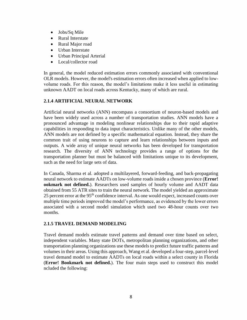
In general, the model reduced estimation errors commonly associated with conventional

OLR models. However, the model's estimation errors often increased when applied to low-

volume roads. For this reason, the model’s limitations make it less useful in estimating

unknown AADT on local roads across Kentucky, many of which are rural.

2.1.4 ARTIFICIAL NEURAL NETWORK

Artificial neural networks (ANN) encompass a consortium of neuron-based models and

have been widely used across a number of transportation studies. ANN models have a

pronounced advantage in modeling nonlinear relationships due to their rapid adaptive

capabilities in responding to data input characteristics. Unlike many of the other models,

ANN models are not defined by a specific mathematical equation. Instead, they share the

common trait of using neurons to capture and learn relationships between inputs and

outputs. A wide array of unique neural networks has been developed for transportation

research. The diversity of ANN technology provides a range of options for the

transportation planner but must be balanced with limitations unique to its development,

such as the need for large sets of data.

In Canada, Sharma et al. adopted a multilayered, forward-feeding, and back-propagating

neural network to estimate AADTs on low-volume roads inside a chosen province (Error!

ookmark not defined.). Researchers used samples of hourly volume and AADT data

obtained from 55 ATR sites to train the neural network. The model yielded an approximate

25 percent error at the 95th confidence interval. As one would expect, increased counts over

multiple time periods improved the model’s performance, as evidenced by the lower errors

associated with a second model simulation which used two 48-hour counts over two

months.

2.1.5 TRAVEL DEMAND MODELING

Travel demand models estimate travel patterns and demand over time based on select,

independent variables. Many state DOTs, metropolitan planning organizations, and other

transportation planning organizations use these models to predict future traffic patterns and

volumes in their areas. Using this approach, Wang et al. developed a four-step, parcel-level

travel demand model to estimate AADTs on local roads within a select county in Florida

(Error! Bookmark not defined.). The four main steps used to construct this model

ncluded the following:

9

1. Network Modeling: The network model was developed using original and

processed data from a range of sources. Centroids and centroid connectors were

placed in each parcel to provide access to adjacent roads.

2. Trip Generation: The model used regression equations from the Institute of

Transportation Engineers (ITE) Trip Generation manual to estimate trips generated

(20). Land-use types corresponding to each parcel in the model area informed the

regression equation selection process.

3. Trip Distribution: The model distributed trips through the gravity model method.

This method distributes trips produced in one zone to other zones in the model (21).

The model assumed each parcel only produced trips but did not attract trips in

relation to other parcels.

4. Trip Assignment: Each vehicle traveling on local roads within the model area

received trip assignments prescribing the chosen travel path. The model assumed

travelers would choose paths that minimized free-flow travel times.

The model utilized ArcGIS and Cube. The final model's results compared favorably with

known AADTs extracted from short-term traffic counts. The model generated mean

absolute errors of 52 percent, considerably lower than the 211 percent from the Zhao and

Chung OLR model.

2.1.6 ORIGIN-DESTINATION (OD) CENTRALITY-BASED METHOD

Typical origin-destination models attempt to predict travel behavior with respect to a

vehicle’s starting point (origin) and end point (destination). Lowry built upon this

conventional method by incorporating the concept of centrality into this framework

(Error! Bookmark not defined.). The Lowry model spatially interpolated AADT for local

treets found in the model area. It used the following equation to describe this relationship:

𝑂𝐷 𝑐𝑒𝑛𝑡𝑟𝑎𝑙𝑖𝑡𝑦𝑒 = ∑ 𝜎𝑖𝑗(𝑒)𝑀𝑖𝑀𝑗

𝑖𝜖𝐼,𝑗𝜖𝐽

Where

i and j are origin and destination nodes

𝜎𝑖𝑗 is the shortest path from origin i to destination j

𝜎𝑖𝑗(𝑒) is equal to 1 if link e is on the path of 𝜎𝑖𝑗, and 0 otherwise

𝑀𝑖 and 𝑀𝑗 are the corresponding multipliers for origin i and destination j

The model used multipliers for specific land-use types, as shown in the ITE Trip

Generation manual. Furthermore, it calculated trip production and attraction rates in a

manner similar to conventional travel demand models. The following inputs were required

for this process:

The street network

The known AADTs

Land use parcels

10

Boundary locations on the street network

Lastly, this model calculated three different origin-destination (OD) centrality measures,

including internal-internal OD centrality, internal-external OD centrality, and external-

external OD centrality. These measures are used as explanatory variables in accompanying

OLR models. The Lowry model produced the highest R-squared values and lowest median

absolute percent errors, respectively, in relation to the models evaluated for this literature

review.

2.1.7 FLORIDA TURNPIKE MODEL

The Florida Department of Transportation uses a statewide transportation model — the

FDOT Turnpike Model — to determine AADTs along its roadways. This model estimates

AADT on all roads including local roads. The model uses the following data as inputs:

Statewide parcel shapefile

Known AADT data shapefile

Employment data from InfoUSA

Selection of Traffic Analysis Zones

HERE Street Network

Once collected, the Turnpike Model divides the roadways found in the HERE street

network into different tiers based on the roadway's functional levels (22). Next, the model

assigns housing and employment units to routes. Housing and employment units (in terms

of number of employees) are converted into trips generated. Finally, trips are assigned

travel routes within the network. Transportation planners can then estimate AADTs based

upon the model's predicted output.

2.2 DISCUSSION AND RECOMMENDATION

The Zhao and Chung OLR method was selected as the modeling approach for estimating

local roadway AADT due to: availability of data, ability to replicate the process, and

availability of resources (chiefly time). Specifically the explanatory variables found in this

model were used to derive the first iteration of a Kentucky-based AADT model, hereafter

referred to as the Broward County model. This model was selected for several reasons.

First, it displayed positive results in estimating local roadway AADT within Broward

County, Florida. Second, it was compatible with existing data accessible across various

KYTC and county databases, thereby eliminating additional time and resource demands

needed in data collection. Finally, the model achieved an optimal balance between roadway

modeling accuracy, user friendliness, and resource requirements, to achieve the desired

effect within reasonable demands (Error! Bookmark not defined.). Other models were

xcluded from further analysis because they were either prone to excessive errors, had

limited compatibility with Kentucky’s roadway network, or imposed too many resource

(e.g., data and time) demands.

11

CHAPTER 3: AADT MODEL

3.1 MODEL DEVELOPMENT

Building upon the state of practice, six unique models were developed to estimate local

roadway traffic volumes in Kentucky. Assessments were performed to judge each model’s

capacity to produce reliable and accurate AADT estimates as well as its ability to use

readily available data. The developed models included two variations on the original

Broward County model (with and without Property Valuation Administrator (PVA) data),

a Rooftop model, a 911 model, and two variations of an AVIS-HERE model (linear and

non-linear regressions). Each model had specific advantages as well as limitations.

Ultimately, the non-linear regression AVIS-HERE model was chosen as the final Kentucky

model for estimating local road traffic counts based upon its accuracy, low error

associations, and availability of data. Section 3.3 describes this model in detail. The other

investigated models are described briefly below and in greater detail in Appendices A - E.

Initially, the Broward County model required modification to align its explanatory

variables with those most closely associated with Kentucky’s local roadway

characteristics. This model was tested on data from Boyd, Clark, Franklin, Green, and

Henry counties. However, the estimative attributes of this model were limited. A graph

comparing estimated AADT with known AADT demonstrated the model’s high error rate.

Thus, the model required additional modifications to improve its effectiveness.

In an effort to enhance the Broward County model, another component was added to it —

PVA data. County governments routinely collect PVA data for residential and commercial

properties within the county limits. PVA data may include information on property owners,

sizes, and addresses, among others. PVA data were incorporated to determine the number

and type of properties located along local roadways and analyze their potential impacts on

AADT. This model demonstrated improvement over the original Broward County version,

with reductions in the magnitude of errors corresponding to the deviation between known

and estimated AADTs. Nonetheless, the errors still exceeded acceptable ranges (100 – 300

percent), thereby excluding it from further consideration.

Next, in an attempt to improve the identification of properties located near local roadways,

the Rooftop model was developed. Properties located along local roads were assumed to

serve as potential traffic generators. To locate properties, ArcGIS was used to identify

rooftops—and by extension, their associated properties—throughout Meade County.

Properties were classified as small, medium, or large, depending on their use. For example,

individual houses were classified as small, while an industrial complex was considered

large. Furthermore, a connectivity rating was assigned to individual roads within the

county. Connectivity ratings ranged from one to six. Higher values indicated greater

connectivity between the individual road and the overall roadway network. The Rooftop

model used these variables to estimate AADT values. However, it did not produce a

measurable improvement in errors over the previous two models. The combination of high

errors along with time constraints imposed by the model’s visual identification

methodology ultimately excluded it as a viable alternative.

12

The 911 model estimated AADT based on the number and location of residential and

commercial properties in Meade County, which were identified in its emergency services,

or 911, database. This approach was similar to the Broward County with PVA model, given

that it leveraged known property addresses. The model assigned residential and

commercial properties to the nearest local roadway, with each property type serving as a

type of trip generator. Testing this model revealed it represented an improvement over

previously developed models, with lower errors found between known and estimated

AADT. Unfortunately, statewide county-level 911 data proved difficult to obtain.

Therefore, this model ended up relying on only a single county for its development and

could not be practically extrapolated to model all counties in Kentucky. A more robust

dataset was needed to provide statewide coverage of properties.

The regression techniques originally used in the 911 model were adapted to develop two

versions of the AVIS-HERE model. Both models relied on a combination of KYTC

statewide data and proprietary HERE data to successfully estimate AADTs. The AVIS-

HERE model has two multivariable forms, ordinary linear regression and non-linear

regression. In the former, the model estimates AADTs as a single statewide model and does

not make the distinction between different regions or districts. Two lane roads classified as

local roads were used to calibrate and validate the models based on known traffic counts.

Additional details on this model’s performance and derivation can be found in Appendix

E. The second AVIS-HERE model used non-linear regression to estimate AADT. This

model outperformed all models in the study with the exception of the 911 model. However,

911 model data was not readily accessible for all counties in Kentucky. Therefore, the non-

linear regression AVIS-HERE model was selected as the Kentucky local roadway AADT

model due to its combined high performance and data availability.

Two sets of models were developed for Kentucky using non-linear regression, one for rural

local roads and one for urban local roads. A separation was made for these road types to

account for the difference in traffic characteristics in these two settings. Section 3.3

includes a detailed discussion of these models and their characteristics.

3.2 DATA COLLECTION

Several data types were used as input into the AVIS-HERE model. The data collected

included: short duration traffic counts, Highway Information System (HIS) variables,

AVIS, and HERE. Short duration traffic counts track the number of vehicles passing a

roadway segment through mechanical means. HIS is a database maintained by KYTC that

includes various characteristics on the highway network including functional classification,

number of lanes, etc. KYTC also provided access to their AVIS database, a collection of

state registration records on all private and commercial vehicles. Finally, HERE

corporation’s probe count data was acquired through the University, which tracks select

smartphones, personal navigation devices, and vehicle fleets. Each data category is

discussed in greater detail below.

13

3.2.1 SHORT DURATION TRAFFIC COUNTS

KYTC strategically and periodically places automatic data recorders (ADRs) along select

roadway segments across the state to collect traffic counts. ADRs typically stay in place

for a minimum of 48 hours (although sometimes longer), but nearly always less than a

week. KYTC primarily uses ADRs to collect data on state roadways directly under its

jurisdiction, but they sometimes capture information on local roads as well. KYTC’s

Division of Planning performs these actions as part of its Traffic Monitoring System in an

effort to better understand the traffic demands and constraints existing along its

transportation network. This information is available to the public through KYTC’s

Interactive Statewide Traffic Counts Map (Figure A).

Figure A: KYTC Traffic Counts, Franklin Co.

Once traffic counts are known, KYTC transportation planners calculate the AADT for each

location. The Division of Planning provided known AADTs along selected local roadways

of interest. Portions of this data were used to validate and calibrate the AADT model

through comparison between estimated and known AADTs.

3.2.2 KYTC AADT DATA

KYTC uses Automatic Traffic Recorders (ADRs) to collect data continuously in order to

develop factors to annualize short duration coverage counts. Planners use this information

to better inform its transportation planning activities as well as meet federal guidelines such

as data collection requirements used for the Highway Performance Monitoring System

(HPMS). KYTC AADT data used in this study consisted of their most recent traffic count

14

cycle of data compiled over the years 2010 through 2013. KYTC AADTs were used to test

and calibrate models.

3.2.3 AVIS DATA

KYTC assesses the values and collects taxes on all vehicles across the state. Each year,

Kentucky vehicle owners must file for continued vehicle registration and provide required,

predetermined information to KYTC along with a fee. KYTC collects and manages this

information through its Automated Vehicle Information System (AVIS). AVIS is an

automated information technology support system used to collect, maintain, and process

motor vehicle registration data. Each County Clerk office initially enters these data into

AVIS through a computer interface. From each of these locations, the data move across the

network into the centralized AVIS mainframe, located in Frankfort, and provides the

KYTC with motor vehicle registration records from across the state.

AVIS data include information related to the vehicle, owner, and the county of record.

Specifically, AVIS data used in this analysis include: vehicle identification number (VIN),

county of registration, year of registration, registration type, and the owner’s address. The

registration type is categorized as official, commercial, or non-commercial. Vehicles

registered as official include those owned by state agencies and organizations, such as

police departments or universities. Commercial vehicles indicate ownership by registered

businesses while non-commercial vehicles are those owned by private citizens (23). A

small sample of AVIS data is shown in Table 2. All vehicle identification numbers (VINs)

and address listings have been replaced with generic identifiers to maintain confidentiality

of the data.

Table 2: AVIS Data

3.2.4 HERE DATA

The HERE corporation, formerly known as NAVTEQ, is an industry leader in geospatial

products, including digital maps. Various digital platforms incorporate this mapping

technology into their consumer products, including cell phones and GPS devices. HERE

uses mapping technology to track vehicle movements through the same cell phones and

GPS devices. The tracking process relies upon cellular towers and antennas located across

much of the nation to collect and monitor cell phone data and GPS signals.

VIN CNTY_REG YEAR_REG REGISTRATION_TYPE ADDR_STREET ADDR_CITY ADDR_STATE ADDR_ZIP

VIN #1 MEAD 15 Non-Commercial Registration ADDRESS #1 EKRON KY 401170000

VIN #2 MEAD 15 Non-Commercial Registration ADDRESS #2 BRANDENBURG KY 401080000

VIN #3 MEAD 15 Commercial Registration ADDRESS #3 BRANDENBURG KY 401080000

VIN #4 MEAD 15 Commercial Registration ADDRESS #4 VINE GROVE KY 401750000

VIN #5 MEAD 15 Commercial Registration ADDRESS #5 BRANDENBURG KY 401080000


VIN #7 MEAD 15 Non-Commercial Registration ADDRESS #7 BATTLETOWN KY 401040000


VIN #10 MEAD 15 Non-Commercial Registration ADDRESS #10 GUSTON KY 401420000

VIN #11 MEAD 15 Official Registration ADDRESS #11 EKRON KY 401170000

VIN #12 MEAD 15 Non-Commercial Registration ADDRESS #12 VINE GROVE KY 401750000

VIN #13 MEAD 15 Official Registration ADDRESS #13 BRANDENBURG KY 401080000

VIN #14 MEAD 15 Non-Commercial Registration ADDRESS #14 EKRON KY 401170000

VIN #15 MEAD 15 Commercial Registration ADDRESS #15 BATTLETOWN KY 401040000

15

HERE uses vehicle tracking data to calculate and monitor vehicular speeds across

roadways. This is accomplished by monitoring the time it takes a vehicle to move along a

predetermined roadway segment. HERE partitions existing roadways into a series of

discrete segments defined by an origin (starting point) and destination (finish point). Each

individual segment corresponds to a distinct “probe” area. Along with calculating average

speeds, HERE collects probe counts from select smartphones, personal navigation devices,

and vehicle delivery transponders (24). These counts, however, do not entirely represent

the traffic on segments. Limitations exist because not every vehicle on the roadway

contains an applicable HERE probe device, and some contain more than one.

HERE probe counts are available in 15-minute intervals for any given day of the week.

HERE initially aggregates its probe data for each day in the month, which produces a daily

count. Next, daily averages are determined for each day of the week. This methodology

combines daily counts across a given month and calculates probe count averages for each

day of the week. For example, a typical June may have four Thursdays. Probe counts are

obtained for each Thursday and averaged into a single Thursday probe count for June. This

single count is subsequently divided into 15-minute intervals. This same methodology is

used for each month of the year. Consequently, a Thursday probe count average in June

might differ from the Thursday probe count average occurring in another month. Probe

count data was acquired from the HERE corporation for the 2012 calendar year (Error!

ookmark not defined.).

3.3 KENTUCKY AADT MODEL

3.3.1 AVIS-HERE NON-LINEAR REGRESSION MODEL

The AVIS-HERE non-linear regression model was selected as the best overall modeling

method due to its ability to accurately estimate AADTs for Kentucky’s local roads while

drawing from accessible and comprehensive data sources. This model relied on property

records contained in the KYTC-sponsored AVIS database as well as the HERE

corporation’s probe counts. As discussed previously, the AVIS database is a motor vehicle

registration database that contains address information on people, commercial businesses,

and governmental agencies that own one or more vehicles registered in the state of

Kentucky. This vehicle registration database allowed for the use AVIS records as a proxy

for residential and commercial properties located in Kentucky. For instance, all addresses

of non-commercial registration records were considered private residences and used to

determine residential properties in this model. Similarly, addresses of commercially-owned

vehicles were designated as commercial properties. A limitation of this model is that it did

not take into account residential and commercial properties owning a vehicle registered

outside of Kentucky. In some instances, it was noted that a small number of vehicles were

registered in Indiana, Tennessee, and other states. Nevertheless, this model should capture

the large majority of passenger car vehicles traveling in Kentucky.

KYTC categorizes AVIS data as proprietary and sensitive due to its ability to match vehicle

identification numbers and addresses to specific individuals and businesses. Therefore, it

16

was agreed to implement appropriate safeguards and protocols when handling this data to

ensure confidentiality and prevent its release. The second data source included probe count

tabulations from the 2012 HERE data set. This data set identifies traffic counts along

roadway segments across the state. The factors used to formulate this model also included

properties, commercial properties, vehicle probe counts, and road curvature. Each factor

used is discussed in more detail below.

3.3.1.1 RESIDENTIAL PROPERTIES

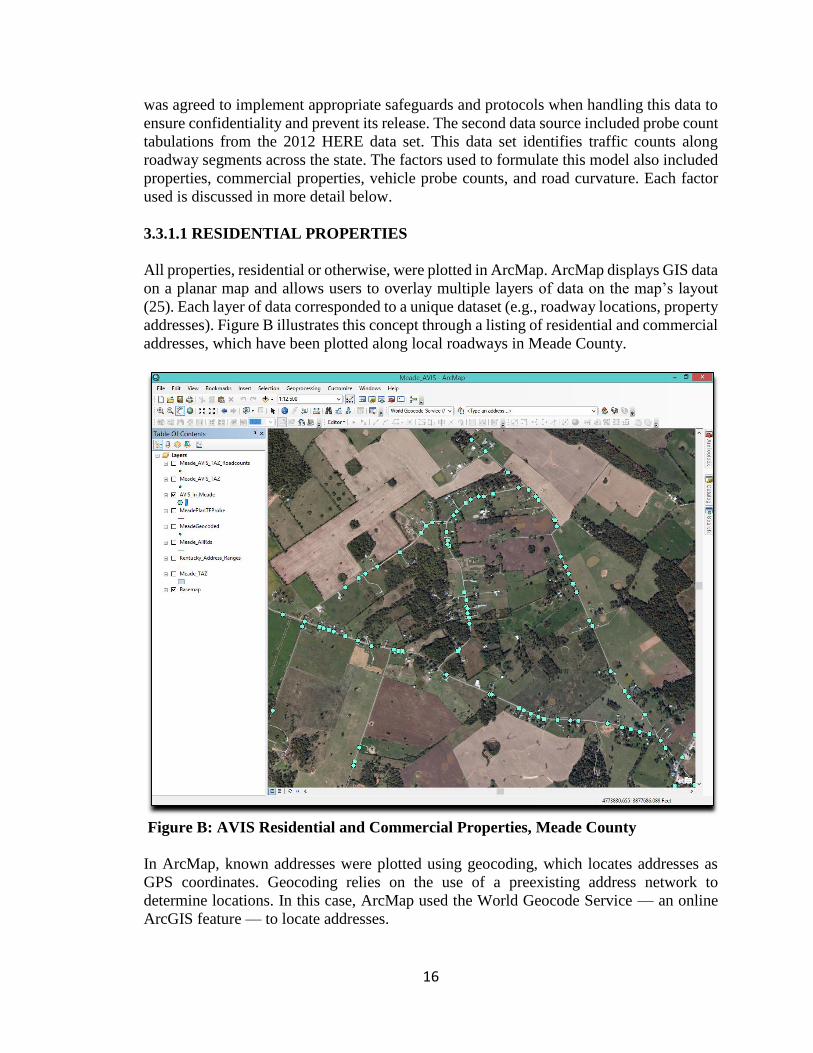
All properties, residential or otherwise, were plotted in ArcMap. ArcMap displays GIS data

on a planar map and allows users to overlay multiple layers of data on the map’s layout

(25). Each layer of data corresponded to a unique dataset (e.g., roadway locations, property

addresses). Figure B illustrates this concept through a listing of residential and commercial

addresses, which have been plotted along local roadways in Meade County.

Figure B: AVIS Residential and Commercial Properties, Meade County

In ArcMap, known addresses were plotted using geocoding, which locates addresses as

GPS coordinates. Geocoding relies on the use of a preexisting address network to

determine locations. In this case, ArcMap used the World Geocode Service — an online

ArcGIS feature — to locate addresses.

17

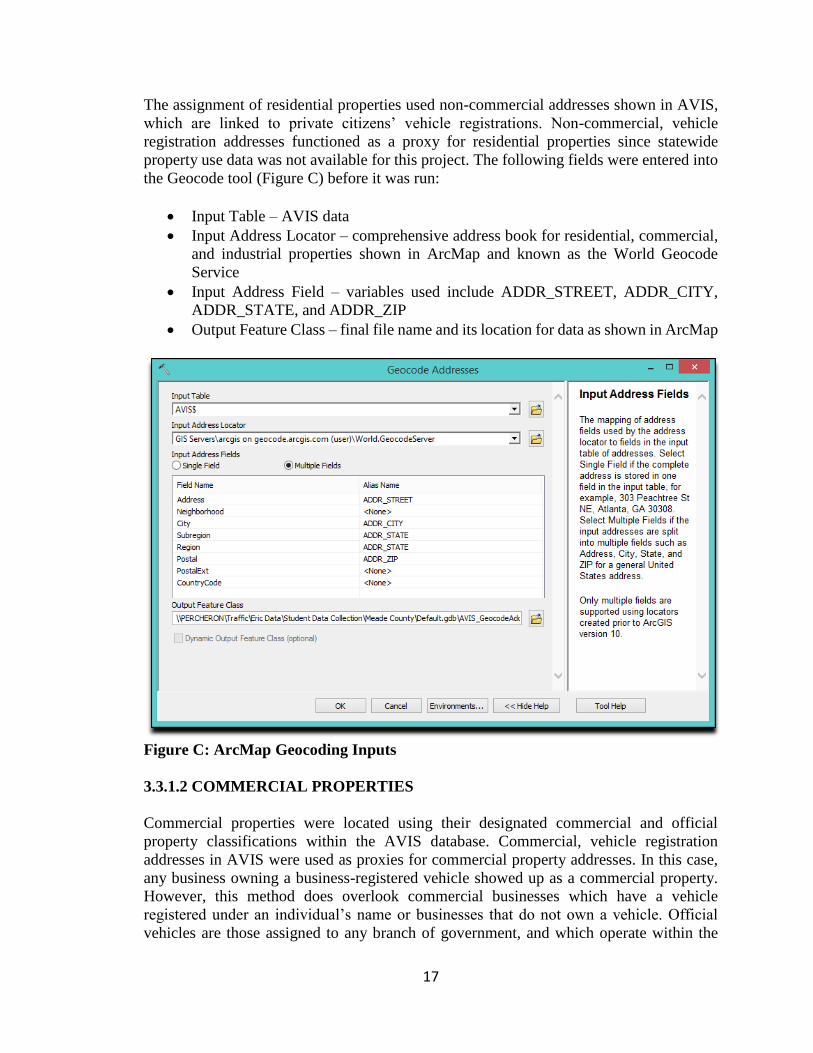
The assignment of residential properties used non-commercial addresses shown in AVIS,

which are linked to private citizens’ vehicle registrations. Non-commercial, vehicle

registration addresses functioned as a proxy for residential properties since statewide

property use data was not available for this project. The following fields were entered into

the Geocode tool (Figure C) before it was run:

Input Table – AVIS data

Input Address Locator – comprehensive address book for residential, commercial,

and industrial properties shown in ArcMap and known as the World Geocode

Service

Input Address Field – variables used include ADDR_STREET, ADDR_CITY,

ADDR_STATE, and ADDR_ZIP

Output Feature Class – final file name and its location for data as shown in ArcMap

Figure C: ArcMap Geocoding Inputs

3.3.1.2 COMMERCIAL PROPERTIES

Commercial properties were located using their designated commercial and official

property classifications within the AVIS database. Commercial, vehicle registration

addresses in AVIS were used as proxies for commercial property addresses. In this case,

any business owning a business-registered vehicle showed up as a commercial property.

However, this method does overlook commercial businesses which have a vehicle

registered under an individual’s name or businesses that do not own a vehicle. Official

vehicles are those assigned to any branch of government, and which operate within the

18

boundaries of Kentucky. These vehicles were also designated as commercial properties due

to their ability to generate higher traffic volumes along assigned roadways. The total

number of official properties is much lower than the number of commercial properties and

does not warrant assignment of an individual variable in this model.

3.3.1.3 PROBE COUNTS

The 2012 HERE probe counts were aggregated for the entire year to produce an annual

traffic count for each roadway segment. The traffic count was then divided by 365 (the

total number of days in a year) to calculate AADT. However, this measure is not a true

AADT because it does not account for all vehicles using the roadway network. HERE only

counts probes from select smartphones, personal navigation devices, and vehicle delivery

fleets. Next, the highway segmentation of the HERE roadway network, which does not use

the same segmentation as the KYTC’s HIS files, was adapted to map the values of HERE

probe counts in ArcMap. The HERE segmentation was then overlaid using the join feature

in ArcMap, which produced an average value of the probe counts for each roadway

segment from the KYTC HIS files.

3.3.1.4 ROADWAY CURVATURE

A value to describe the curvature of each road segment was calculated by determining the

actual length of the road segment and the straight length between the end points of the road

segment. The ratio of the actual length to the straight length of the road is the curve rating,

and it was used as an input variable for the model. The curve rating was included in the

model because roads designed with low anticipated AADTs would not have the adequate

funding needed to make roads straight. Thus, low-volume roadways tend to be more

sinuous than high-volume ones. An inverse relationship was expected between a road

segment’s curve rating and its AADT.

Two separate AVIS-HERE non-linear regression models were developed in this effort,

including a rural- and an urban-based models. Developing two distinct models allowed for

differentiation between conditions typically associated with rural and urban areas,

respectively. The urban and rural models, their development, and underlying results are

described in greater detail in the following sections.

3.3.2 RURAL MODEL DEVELOPMENT

The rural models were developed using short duration traffic counts, residential and

commercial property locations, and HERE probe counts. Each variable required

assignment to a defined roadway segment. In the initial step, defined roadway segments

from KYTC’s HIS database via the ArcMap-based Traffic Flow (TF) file were obtained

(26). This file contains roadway segments for all-type roads across the state, totaling

152,388 segments. The complete list of roadway segments includes state-maintained and

non-state maintained roads (typically local routes). Small, black dots divided the roadway

into its partitioned segments. To illustrate, Figure D displays a small area within Franklin

County, including U.S. Route 127, County Route 1036, and County Route 1039, and their

19

corresponding delineated segments. This figure includes five labels identifying the

segments.

Figure D: KYTC Roadway Segments

Additional modifications were performed to the original KYTC roadway segment file to

better differentiate between state-maintained and local roadway segments. This added

segmentation step employed the “planarized lines” function in ArcMap to divide local

roadways into a larger number of segments. Local roadways were divided into two distinct

segments where they intersect with state-maintained roadways (previously it was a single,

continuous segment). This step improved the accuracy of the model as it assigned discrete

AADTs to both sides of the partitioned local roadway. This process resulted in a total of

167,236 roadway segments in Kentucky, an increase of nearly 10 percent over the original

KYTC file count. Figure E illustrates the same area of Franklin County depicted in Figure

D, but using the modified segmentation process. The map now captures six distinct

segments, or one more than the previously employed segmentation process.

20

Figure E: Modified Roadway Segments

In the final step, HERE probe counts were incorporated into the segmentation process.

HERE has delineated their own unique roadway segments across the state, which

correspond with their probe counts (see Section 3.2.4 for a description of this process).

HERE’s number of roadway segments vastly exceeds the counts of KYTC’s original model

and the modified version, with a total of 514,293 segments. In Figure F, the number of

roadway segments identified through probe counts is displayed for the same area as shown

in Figures D and E. The number of segments increased to 11 for this map.

21

Figure F: HERE Probe Data Segments

The geocoding process converts a table of addresses into a set of coordinates that can be

mapped in ArcMap. Once mapped, they are treated as distinct entities (e.g., individual

properties). Points maintain attributes from the AVIS database. Therefore, each point is

also categorized as official, commercial, or non-commercial.

The roadway network file containing the HERE probe count averages was joined to the

Traffic Flow (TF) file from the KYTC HIS database. This created a new shapefile

comprising all roadway along with the average probe count and known traffic counts. At

this point the straight length of each road segment was calculated using the coordinates of

the beginning and end points of each road segment. Actual road segment lengths were also

calculated. Both calculations were performed using ArcMAP’s “calculate geometry” tool.

The ratio of actual road length to the straight length was calculated for each segment.

Each address coordinate then had information about the nearest roadway segment joined

to it, creating a shapefile of points with the following information:

AVIS registration type: official, commercial, or non-commercial

Unique ID of the roadway segment nearest to the point

Average probe count associated with the nearest roadway segment

22

State traffic count (the count was 0 for local roads)

Curve rating

The shapefile of points with associated roadway segment information was exported into

Excel to convert the data from point format to a polyline format. Each road segment, along

with its associated traffic and probe count, was placed in a separate sheet. To populate the

Residential variable for each roadway segment, the “countifs” function in Excel was

executed such that it only counted the points for each road segment that were registered as

non-commercial and had the nearest road segment with same unique ID as the segment in

question. The Commercial variable was calculated in a similar manner, except it counted

points registered as commercial or official.

Several types of regression were attempted with four variables (commercial and residential

registrations, probe count and curve rating), including ordinary multiple linear regression,

log transformed multiple linear regression, and generalized linear regression. During model

development, it was observed that many commercial properties had no vehicles registered

to those locations. As such, the commercial variable was excluded from the model. After

comparing errors among the different regression types, it was decided that a generalized

linear model with a Poisson distribution and a log link function best fit the data. This type

of model has the following format:

𝑌 = 𝑒𝛼+𝛽1𝑋1+⋯+𝛽𝑛𝑋𝑛

Where

𝑌 is the dependent variable

𝑒 is Euler’s number

𝛼 is the calibrated constant

𝛽𝑛 are the calibrated coefficients

𝑋𝑛 are the explanatory variables

𝑛 is the number of variables

To account for the spatial and socioeconomic variations across Kentucky, the state was

divided into three regions based on the highway districts. The regions and their respective

highway districts were:

West: 1, 2, 3, 4

North Central: 5, 6, 7

East: 8, 9, 10, 11, 12

One model was calibrated for each region. Certain restrictions were placed on the data used

to calibrate each region to ensure that the calibration data closely matched the

characteristics of the roads for which the models would be used to estimate AADT. The

data used to calibrate the models were known traffic counts conducted by KYTC on rural,

state-maintained roads that were functionally classified as local roads. Only roads with

traffic counts between 20 and 1000 were included in the analysis. Several roads with known

traffic counts from KYTC had AADT values ranging from 6 to 19, which appeared

23

inconsistent with numbers reported on an official traffic count. There may have been some

errors in the collection or reporting of these counts. Because of this, they were left out of

the model calibration to avoid introducing bias toward low AADT estimates. The upper

limit of 1000 was established because it was assumed that no rural local roads in Kentucky

lacking a known count would have daily traffic volumes exceeding 1000, given that the

standard definition of a local road is one with an AADT of 400 or fewer. Of the road

segments in each region that fit these criteria, 75 percent were used to calibrate the model.

The remaining 25 percent in each region were used to validate the model.

3.3.3 RURAL MODEL RESULTS

The rural models were developed using Poisson distributed non-linear regression with a

log link function in JMP 12.1, a statistical software package. The three model variables

included probe count (Probe), curve rating (Curve), and residential AVIS registrations

(Residential). Seventy-five percent of each region’s data set was randomly selected to

calibrate the model. Table 3 shows the calibrated coefficients for each model, with the

model taking the following form:

𝐴𝐴𝐷𝑇 = 𝑒𝛼+𝛽1𝑃𝑟𝑜𝑏𝑒+𝛽2𝐶𝑢𝑟𝑣𝑒+𝛽3𝑅𝑒𝑠𝑖𝑑𝑒𝑛𝑡𝑖𝑎𝑙

Table 3: Rural Regional Model Coefficients

Model 𝛼 𝛽1, Probe 𝛽2, Curve 𝛽3, Residential

West 5.7696115 0.0058785 -0.529959 0.0040769

North-Central 5.2644224 0.0057724 -0.077597 0.0055012

East 5.5054758 0.0056975 -0.015072 0.0023554

Each regional model, and its explanatory variables, was statistically significant at the 0.01

percent confidence level. Hence, regional explanatory variables were useful in accounting

for the variation in AADT. Coefficient signs (positive or negative) for each model were

calibrated as expected. Both Probe and Residential variables have positive coefficients.

This meant an increased probe count or residential vehicle registration along a road

segment would produce a higher AADT estimate. The Curve coefficient is negative, which

indicates curvier roads have lower AADTs. It was anticipated that the Curve variable

would have this effect when they decided to incorporate it into the model.

Next, each model’s AADT estimative capability was tested by using the remaining 25

percent of the data set for validation. This step compared estimated AADTs within each

calibrated model with their respective known AADTs, as contained in the regional

validation data sets. This occurred for each highway segment and generated several error

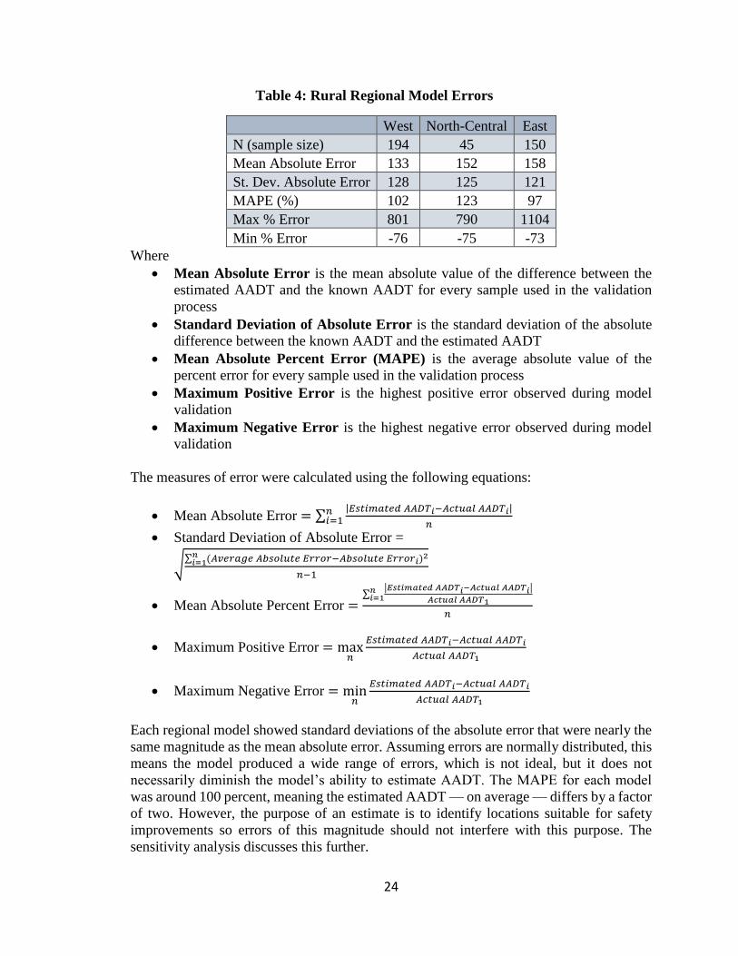
measures. Table 4 summarizes the error measures from the regional models’ validation

data.

24

Table 4: Rural Regional Model Errors

West North-Central East

N (sample size) 194 45 150

Mean Absolute Error 133 152 158

St. Dev. Absolute Error 128 125 121

MAPE (%) 102 123 97

Max % Error 801 790 1104

Min % Error -76 -75 -73

Where

Mean Absolute Error is the mean absolute value of the difference between the

estimated AADT and the known AADT for every sample used in the validation

process

Standard Deviation of Absolute Error is the standard deviation of the absolute

difference between the known AADT and the estimated AADT

Mean Absolute Percent Error (MAPE) is the average absolute value of the

percent error for every sample used in the validation process

Maximum Positive Error is the highest positive error observed during model

validation

Maximum Negative Error is the highest negative error observed during model

validation

The measures of error were calculated using the following equations:

Mean Absolute Error = ∑|𝐸𝑠𝑡𝑖𝑚𝑎𝑡𝑒𝑑 𝐴𝐴𝐷𝑇𝑖−𝐴𝑐𝑡𝑢𝑎𝑙 𝐴𝐴𝐷𝑇𝑖|

𝑛

𝑛𝑖=1

Standard Deviation of Absolute Error =

√∑ (𝐴𝑣𝑒𝑟𝑎𝑔𝑒 𝐴𝑏𝑠𝑜𝑙𝑢𝑡𝑒 𝐸𝑟𝑟𝑜𝑟−𝐴𝑏𝑠𝑜𝑙𝑢𝑡𝑒 𝐸𝑟𝑟𝑜𝑟𝑖

𝑛𝑖=1 )2

𝑛−1

Mean Absolute Percent Error =∑

|𝐸𝑠𝑡𝑖𝑚𝑎𝑡𝑒𝑑 𝐴𝐴𝐷𝑇𝑖−𝐴𝑐𝑡𝑢𝑎𝑙 𝐴𝐴𝐷𝑇𝑖|

𝐴𝑐𝑡𝑢𝑎𝑙 𝐴𝐴𝐷𝑇1

𝑛𝑖=1

𝑛

Maximum Positive Error = max𝑛

𝐸𝑠𝑡𝑖𝑚𝑎𝑡𝑒𝑑 𝐴𝐴𝐷𝑇𝑖−𝐴𝑐𝑡𝑢𝑎𝑙 𝐴𝐴𝐷𝑇𝑖


Maximum Negative Error = min𝑛

𝐸𝑠𝑡𝑖𝑚𝑎𝑡𝑒𝑑 𝐴𝐴𝐷𝑇𝑖−𝐴𝑐𝑡𝑢𝑎𝑙 𝐴𝐴𝐷𝑇𝑖


Each regional model showed standard deviations of the absolute error that were nearly the

same magnitude as the mean absolute error. Assuming errors are normally distributed, this

means the model produced a wide range of errors, which is not ideal, but it does not

necessarily diminish the model’s ability to estimate AADT. The MAPE for each model

was around 100 percent, meaning the estimated AADT — on average — differs by a factor

of two. However, the purpose of an estimate is to identify locations suitable for safety

improvements so errors of this magnitude should not interfere with this purpose. The

sensitivity analysis discusses this further.

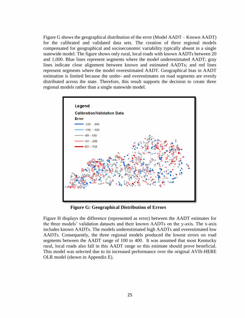
25

Figure G shows the geographical distribution of the error (Model AADT – Known AADT)

for the calibrated and validated data sets. The creation of three regional models

compensated for geographical and socioeconomic variability typically absent in a single

statewide model. The figure shows only rural, local roads with known AADTs between 20

and 1,000. Blue lines represent segments where the model underestimated AADT; gray

lines indicate close alignment between known and estimated AADTs; and red lines

represent segments where the model overestimated AADT. Geographical bias in AADT

estimation is limited because the under- and overestimates on road segments are evenly

distributed across the state. Therefore, this result supports the decision to create three

regional models rather than a single statewide model.

Figure G: Geographical Distribution of Errors

Figure H displays the difference (represented as error) between the AADT estimates for

the three models’ validation datasets and their known AADTs on the y-axis. The x-axis

includes known AADTs. The models underestimated high AADTs and overestimated low

AADTs. Consequently, the three regional models produced the lowest errors on road

segments between the AADT range of 100 to 400. It was assumed that most Kentucky

rural, local roads also fall in this AADT range so this estimate should prove beneficial.

This model was selected due to its increased performance over the original AVIS-HERE

OLR model (shown in Appendix E).

26

Figure H: Validation Errors in Three Regional Models

Figures I, J, and K display known versus estimated AADTs for each Kentucky region. An

ideal estimate would form a 45 degree line demonstrating alignment between known and

estimated AADTs. This hypothetical line is shown in each figure. Data points above the

line represent segments where the model overestimated AADT and points below the line

represent segments where the model underestimated AADT. Greater distances between the

points and the line represent greater errors.

Figure I: West Regional Model, Known vs. Model AADT

-800

-600

-400

-200

0

200

400

0 200 400 600 800 1000 1200

Erro

r (E

stim

ate

-Kn

ow

n A

AD

T)

Known AADT

Comparison of Error Across Calibrated AADT Range

0

50

100

150

200

250

300

350

400

450

500

0 200 400 600 800 1000

Mo

del

AA

DT

Known AADT

West Regional Model

27

Figure J: North-Central Regional Model, Known vs. Model AADT

Figure K: East Regional Model, Known vs. Model AADT

Each model contained a baseline AADT which represented the minimum value the model

could estimate. This baseline was approximately 100 for the West and North-Central

models and approximately 200 for the East model. The calibrated constant 𝛼 was

responsible for this baseline since it remained constant as other explanatory variables

moved to zero. Each model produced higher errors as AADT estimates increase.

Nevertheless, these regional models focused on rural, local roadways – which typically

have lower AADTs—so the higher range AADT errors were not cause for concern.

Next, KYTC’s daily vehicle miles traveled (DVMT) estimate for rural, local roads were

collected and compared those values to each model’s AADT estimates. DVMT is

0

100

200

300

400

500

600

0 200 400 600 800 1000 1200

Mo

del

AA

DT

Known AADT

North-Central Regional Model

0

100

200

300

400

500

600

700

0 200 400 600 800 1000

Mo

del

AA

DT

Known AADT

East Regional Model

28

determined by multiplying a local road segment’s distance (in miles) with its AADT and

represents the total number of vehicle miles traveled along a given roadway segment daily.

KYTC employs a power function to estimate DVMT for rural, local roads. County collector

AADTs serve as explanatory variables in this model which can be described as follows

(27):

𝐿𝑜𝑐𝑎𝑙 𝐷𝑉𝑀𝑇 = 𝐿𝑜𝑐𝑎𝑙 𝑀𝑖𝑙𝑒𝑠 ∗ 𝐿𝑜𝑐𝑎𝑙 𝐴𝐴𝐷𝑇, 𝑤ℎ𝑒𝑟𝑒 𝐿𝑜𝑐𝑎𝑙 𝐴𝐴𝐷𝑇= 3.3439 ∗ (𝐶𝑜𝑙𝑙𝑒𝑐𝑡𝑜𝑟 𝐴𝐴𝐷𝑇)0.6248

Each rural, local DVMT estimate was calculated at the roadway segment level and

aggregated county-wide to produce a county-level DVMT value, the same scale used in

the regional models. The DVMT values served as a basis of comparison with the regional

model AADT estimates. In most instances, the models produced higher DVMT values than

the KYTC DVMT estimates. Ratios by county of the KYTC DVMT estimated values to

the model’s estimated AADTs is shown in Figure L. A brief discussion of this adjustment

methodology is described in the subsequent paragraphs.

Figure L: VMT Adjustment Ratio by County

The KYTC DVMT to model DVMT ratio was used as an adjustment factor in the model’s

AADT estimates. For example, a ratio of 0.75 would be multiplied by the estimated AADT

to further refine the estimate. The majority of adjustment factors were found to be less than

one. This meant that the model DVMT estimates tended to exceed KYTC DVMT values.

29

The lowest adjustment ratios were found in population and urban areas, such as northern

Kentucky. These regions typically have increased cell phone coverage which leads to an

increase in vehicle probe counts (HERE data). The increased population density and

proximity to local roads also contributed to higher residential variable values. Therefore,

the rural, local AADT road estimates in these counties typically exceeded rural, local

AADT road estimates in less populated counties. This, in turn, produced higher DVMT

values for the model estimates compared to the KYTC DVMT values. In Figure L, counties

in pink and red show counties where the KYTC DVMT values exceeded the model’s

DVMT estimates; conversely, blue counties show locations where the KYTC DVMT

values fell below the model’s estimates. The latter case represented the majority of

counties fitting this description.

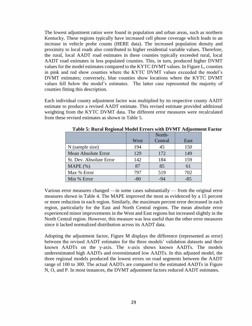
Each individual county adjustment factor was multiplied by its respective county AADT

estimate to produce a revised AADT estimate. This revised estimate provided additional

weighting from the KYTC DVMT data. The different error measures were recalculated

from these revised estimates as shown in Table 5.

Table 5: Rural Regional Model Errors with DVMT Adjustment Factor

West

North-

Central East




MAPE (%) 87 85 61

Max % Error 797 519 702

Min % Error -80 -94 -85

Various error measures changed —in some cases substantially — from the original error

measures shown in Table 4. The MAPE improved the most as evidenced by a 15 percent

or more reduction in each region. Similarly, the maximum percent error decreased in each

region, particularly for the East and North Central regions. The mean absolute error

experienced minor improvements in the West and East regions but increased slightly in the

North Central region. However, this measure was less useful than the other error measures

since it lacked normalized distribution across its AADT data.

Adopting the adjustment factor, Figure M displays the difference (represented as error)

between the revised AADT estimates for the three models’ validation datasets and their

known AADTs on the y-axis. The x-axis shows known AADTs. The models

underestimated high AADTs and overestimated low AADTs. In this adjusted model, the

three regional models produced the lowest errors on road segments between the AADT

range of 100 to 300. The actual AADTs are compared to the estimated AADTs in Figure

N, O, and P. In most instances, the DVMT adjustment factors reduced AADT estimates.

30

Figure M: Validation Errors in Three Regional Models (w/ Adjustment

Factor)

The combined errors graph for the three models (Figure M) displays a similar trend as

previously shown in Figure H. Recall, the previous error graph did not account for the

adjustment factor per the KYTC DVMT data. Nevertheless, the newly revised errors

were nearly zero in the 100 to 300 AADT range, an ideal parameter for the rural, local

roads. The revised model continued to underestimate AADTs for roads with higher

known AADTs but these roads typically lie outside the AADT range expected for rural,

local roads. Therefore, improving model errors across the lower AADT ranges remained

the focus as achieved here.

-1000

-800

-600

-400

-200

0

200

400

0 200 400 600 800 1000 1200Erro

r (E

stim

ated

-Kn

ow

n A

AD

T)

Known AADT

Comparison of Error Across Calibrated AADT Range with Adjustment Factor

31

Figure N: West Regional Model, Known vs Model AADT (w/

Adjustment)

Figure O: North-Central Regional Model, Known vs Model AADT (w/

Adjustment)

0

50

100

150

200

250

300

350

400

450

500

0 200 400 600 800 1000

Mo

del

AA

DT

Known AADT

West Regional Model (Adjusted)

0

50

100

150

200

250

300

350

400

450

500

0 200 400 600 800 1000

Mo

del

AA

DT

Actual AADT

North Central Adjusted AADT Model

32

Figure P: East Regional Model, Known vs Model AADT (w/ Adjustment)

Next, known AADTs were graphed against estimated AADTs for each of the regional

models (Figures N, O, P). The minimum estimated AADT decreased by a factor of two for

each model. Thus, these regional models improved the alignment between known and

estimated AADTs, as represented by an increased number of points moving closer to the

45 degree graph line. Each county possessed a unique adjustment factor and therefore, was

adjusted independently from other counties. This lead to increased variation in the model

AADT estimates. This can be seen by an increase in scatter between points amongst

Figures N, O, and P compared to Figures I, J, and K.

3.3.4 URBAN MODEL DEVELOPMENT

The urban AADT model was created using a similar methodology as that employed in the

rural AADT models development. To this extent, the urban models used the same

segmentation process for subdividing roadways as described in detail in section 3.3.2. The

urban model consisted of the same three variables (probe count, curve rating, and

residential AVIS registrations) derived from the same data sets. Once again, this model

split the state into three separate geographical regions (West, North-Central, and East)

using the same procedures shown in developing the rural model. 75% of the AADT data

in each region was used to calibrate the model and the remaining 25% of data to validate

the model. However, there was one major methodological difference between the rural

and urban model development. The original rural AADT model required road segments

with a known AADT between 20 and 1,000, while no such limitation was placed on the

calibration data set for the urban model. In fact, urban traffic counts span a wide range of

values and limitations on the calibrated datasets were not deemed necessary.

0

50

100

150

200

250

300

350

400

450

500

0 200 400 600 800 1000

Mo

del

AA

DT

Known AADT

East Regional Model (Adjusted)

33

3.3.5 URBAN MODEL RESULTS

The urban models were calibrated using Poisson distributed non-linear regression with a

log link function in JMP 12.1, in a similar fashion to the rural models. The three model

variables included probe count (Probe), curve rating (Curve), and residential AVIS

registrations (Residential). Table 6 shows the calibrated coefficients for each model, with

the model taking the following form:

𝐴𝐴𝐷𝑇 = 𝑒𝛼+𝛽1𝑃𝑟𝑜𝑏𝑒+𝛽2𝐶𝑢𝑟𝑣𝑒+𝛽3𝑅𝑒𝑠𝑖𝑑𝑒𝑛𝑡𝑖𝑎𝑙

Table 6: Urban Regional Model Coefficients

Model 𝛼 𝛽1, Probe 𝛽2, Curve 𝛽3, Residential

West 6.470643 0.0064529 -0.125808 0.0028887

North-Central 5.8138784 0.0112211 0.2191382 0.0115388

East 7.0093157 0.0072614 -0.079176 0.0002173

Each regional model, and its explanatory variables, was statistically significant at the 0.01

percent confidence level. Hence, regional explanatory variables were useful in accounting

for the variation in AADT. Coefficient signs (positive or negative) for each model

performed as expected for all but one coefficient. Both Probe and Residential variables had

positive coefficients. This meant an increased probe count or residential vehicle

registration along a road segment produced a higher AADT estimate. The Curve

coefficient was negative for the West and East models, which indicated curvier roads have

lower AADTs. However, the Curve coefficient in the North-Central model was positive,

which ran contrary to the results of the West and East models. Nonetheless, dividing the

state into three regions limited the overall effect this positive coefficient had on the

cumulative urban AADT estimates for the state.

The same error metrics were calculated as before as suitable measures of effectiveness.

Table 7 summarizes these error types and their associated valuations from the urban

regional models’ validation data.

Table 7: Urban Regional Models Errors





MAPE (%) 1956 1828 354

Max % Error 16878 11070 8278

Min % Error -79 -63 -81

The Table 7 summary results demonstrate the urban models had much higher errors when

compared to the rural models. One possible explanation for this may be the higher

variability of AADT values used to calibrate the urban models. Also, the urban model

34

relied upon a smaller available dataset to calibrate each regional model which likely

impacted the model’s effectiveness.

The KYTC-provided DVMT values were used as control totals to develop adjustment

factors and modify the urban models’ AADT estimates. However the calculations used to

derive control totals differed between the urban models and the rural models. In the rural

models, the DVMT adjustment factor represented the ratio between KYTC-derived rural

DVMT values for a county and rural DVMT model estimates for the same county. This

adjustment factor was applied to each rural local road segment in the county. In the urban

models, adjustment factors were calculated differently based on the following two

scenarios: the model-derived DVMT was less than the KYTC-derived DVMT or the

model-derived DVMT was greater than the KYTC-derived DVMT. For the first scenario,

adjustments were made to urban local roads found to intersect state roads when the

county’s model-derived DVMT was less than the KYTC-derived DVMT using an

adjustment factor that increased AADT on roads that intersect state roads. With the second

the urban local roads that do not intersect state roads received DVMT adjustments if the

county’s model DVMT exceeded the Cabinet’s DVMT value, thereby reducing the urban

local road AADT values.

The purpose of creating adjustment factors in this manner was to avoid assigning additional

AADT on neighborhood roads that only connect to other local roads while assigning

increased AADT on roads that contribute more heavily to state roads. An example

adjustment factor calculation for each described case scenarios shown below (and based

on the DVMT data in Table 8).

Table 8: Urban DVMT Control Total Data

County

DVMT do not

intersect state

DVMT intersect

state

KYTC

DVMT

Adjustment

Factor

Anderson 7361 6529 55000 7.30

Pike 14367 28707 37000 0.58

The urban AADT model estimated AADT values that lead to a lower DVMT (combined

intersect and do not intersect) in Anderson County than estimated by KYTC in 2014.

Therefore, an adjustment factor was needed to increase AADT on the urban, local roads

that intersect state roads. The adjustment factor was calculated as follows:

𝐴𝑑𝑗𝑢𝑠𝑡𝑚𝑒𝑛𝑡 𝐹𝑎𝑐𝑡𝑜𝑟 =𝐶𝑎𝑏𝑖𝑛𝑒𝑡 𝐷𝑉𝑀𝑇 − 𝐷𝑉𝑀𝑇 𝑛𝑜𝑡 𝑖𝑛𝑡𝑒𝑟𝑠𝑒𝑐𝑡𝑖𝑛𝑔 𝑠𝑡𝑎𝑡𝑒 𝑟𝑜𝑎𝑑𝑠

𝐷𝑉𝑀𝑇 𝑖𝑛𝑡𝑒𝑟𝑠𝑒𝑐𝑡𝑖𝑛𝑔 𝑠𝑡𝑎𝑡𝑒 𝑟𝑜𝑎𝑑𝑠

=(55000 − 7361)

6529= 7.30

This factor holds constant the AADT on local roads that do not intersect state roads while

increasing AADT on local roads that intersect state roads to 47662.

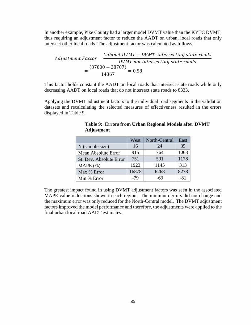
35

In another example, Pike County had a larger model DVMT value than the KYTC DVMT,

thus requiring an adjustment factor to reduce the AADT on urban, local roads that only

intersect other local roads. The adjustment factor was calculated as follows:

𝐴𝑑𝑗𝑢𝑠𝑡𝑚𝑒𝑛𝑡 𝐹𝑎𝑐𝑡𝑜𝑟 =𝐶𝑎𝑏𝑖𝑛𝑒𝑡 𝐷𝑉𝑀𝑇 − 𝐷𝑉𝑀𝑇 𝑖𝑛𝑡𝑒𝑟𝑠𝑒𝑐𝑡𝑖𝑛𝑔 𝑠𝑡𝑎𝑡𝑒 𝑟𝑜𝑎𝑑𝑠

𝐷𝑉𝑀𝑇 𝑛𝑜𝑡 𝑖𝑛𝑡𝑒𝑟𝑠𝑒𝑐𝑡𝑖𝑛𝑔 𝑠𝑡𝑎𝑡𝑒 𝑟𝑜𝑎𝑑𝑠

=(37000 − 28707)

14367= 0.58

This factor holds constant the AADT on local roads that intersect state roads while only

decreasing AADT on local roads that do not intersect state roads to 8333.

Applying the DVMT adjustment factors to the individual road segments in the validation

datasets and recalculating the selected measures of effectiveness resulted in the errors

displayed in Table 9.

Table 9: Errors from Urban Regional Models after DVMT

Adjustment





MAPE (%) 1923 1145 313

Max % Error 16878 6268 8278

Min % Error -79 -63 -81

The greatest impact found in using DVMT adjustment factors was seen in the associated

MAPE value reductions shown in each region. The minimum errors did not change and

the maximum error was only reduced for the North-Central model. The DVMT adjustment

factors improved the model performance and therefore, the adjustments were applied to the

final urban local road AADT estimates.

36

CHAPTER 4: SENSITIVITY ANALYSIS

4.1 SENSITIVITY ANALYSIS

Estimative models inherently rely on engineering judgment and analytical assumptions.

These are incorporated into the models’ algorithms to compute the desired outputs. In some

cases, however, a model may estimate values that do not align with expected empirical

solutions. This requires the model developer to perform additional checks and/or validation

procedures to further improve its performance. Sensitivity analysis is one procedure that

can be used to improve results. A sensitivity analysis measures how a model’s output (or

dependent variable) is expected to change based upon the explanatory factors (or

independent variables) used to develop it. This process provides an additional check on

uncertainty or the model’s assumptions and determines how they might impact the

predicted solutions. One of the key goals of a sensitivity analysis is to minimize any

unexpected or adverse outcomes stemming from a less-than-satisfactory output. This

process helps ensure that the model’s inaccuracies do not have an overly adverse impact

on the output. Following this process, a sensitivity analysis was developed to analyze the

selected AADT traffic model and its expected range of impacts on crash predictions,

including their severity.

4.1.1 KYTC CRASHES AND ASSOCIATED COSTS

KYTC seeks the use of an AADT traffic model to estimate traffic counts on local roads

across the state. These values are critical to KYTC for a number of reasons, including

providing a means to predict crashes along a roadway segment or at an intersection. KYTC

uses crash data to evaluate safety measure installations. Roadway segments or intersections

experiencing a large number of crashes warrant additional scrutiny to decide whether

increased funding might reduce crash frequency. In some cases, the installation of safety

measures at an appropriate roadway segment or intersection may significantly lower the

number of crashes within that area. In other cases, the installation of the safety measures

may have a negligible impact and therefore provide little benefit at a potentially high

financial cost. Intuitively, it is in KYTC’s interest to prioritize locations where treatments

will provide the greatest return on investment while avoiding areas where treatments will

yield minimal benefits at a significant cost. State DOTs take their lead from the U.S. DOT

to provide safe roadways to all their citizens. In fact, a significant percentage of overall

federal highway funding is dedicated exclusively to reducing crashes. This aligns with the

U.S. DOT’s 2012-2016 Strategic Plan “Transportation for a New Generation” and their

goal to “improve public health and safety by reducing transportation-related fatalities and

injuries.” (28)

KYTC leaders and decision-makers must rely on sound estimates and projections whenever

determining which roadways or intersections need safety treatments. Likewise, roadway

sites receive a prioritization ranking based on the expected benefits of installing a safety

measure. To compare the effects of measures at different sites, the FHWA has developed

crash costs, which are estimated based on the crash severity in terms of human life and

property damage. The categories or types of crash severity are: fatal, disabling injury,

37

evident injury, possible injury, and property damage only. Each of these categories is

assigned a corresponding monetary value (in dollars), which quantifies impacts financially.

Along with the crash types, the crash costs are further delineated according to human

capital crash costs and comprehensive crash costs. The human capital crash costs category

only includes financial losses directly associated with the crash, such as vehicle repair and

medical treatment, among others. The comprehensive crash costs category takes this a step

further and assigns a monetary value to the burdens imposed on the individual’s quality of

life due to time lost during recovery or potential physical limitations attributable to the

crash. Table 10 lists the FHWA’s crash cost estimates (29).

Table 10: FHWA Crash Cost Estimates by Crash Severity

Crash Type Human Capital

Crash Costs

Comprehensive

Crash Costs

Fatal (K) $1,245,600 $4,008,900

Disabling Injury (A) $111,400 $216,000

Evident Injury (B) $41,900 $79,000

Possible Injury (C) $28,400 $44,900

Property Damage Only (O) $6,400 $7,400

4.1.2 SENSITIVITY ANALYSIS METHODOLOGY

A sensitivity analysis was performed to assess how the model’s estimated local road AADT

values potentially impact crash estimates when accounting for errors. Safety performance

functions (SPFs) are used to estimate crashes, and for this project, were taken from the

Highway Safety Manual (HSM). SPF equations rely upon AADTs as input variables, in

our case, a known AADT for the state road and an estimated AADT for the local road. This

sensitivity analysis used the models’ maximum and minimum percent errors to estimate

AADT estimation error impact on predicted crashes.

First, all intersections in Kentucky were located via the GIS platform. Intersections were

selected so they would match the data set used in the AADT model. The types of

intersections were subsequently categorized into three groups, including:

State-maintained roadways intersecting state-maintained roadways (State-State)

State-maintained roadways intersecting local roadways (State-Local)

Local roadways intersecting local roadways (Local-Local)

All intersections forming a state-to-local roadway crossing (State-Local) formed the basis

of the sensitivity analysis. Intersections were then classified based on their characteristics.

These were used to determine the appropriate HSM regression equations used in the

analysis. For intersections, the factors considered included:

38

Rural or urban roads

Number of intersection approaches (three versus four)

Unsignalized or signalized

Number of lanes in each direction

Roadway characteristics provide transportation planners the details required when

selecting the appropriate regression equations to use. Furthermore, each regression

equation is only suitable for a specified range of traffic volumes. In this sensitivity analysis,

all of the traffic volumes on the major and minor roadways approaching intersections fell

within the acceptable ranges. Therefore, no additional modifications to the regression

equations were required.

Next, the AADTs were used in the sensitivity analysis. Known AADT is available from

HIS for the major crossing or state road. Conversely, the AADT for the local intersecting

roadway is estimated from the AVIS-HERE model. Once the AADTs and roadway

characteristics are known, the SPF can be evaluated and crash estimates produced.

4.1.3 RURAL MODEL SENSITIVITY ANALYSIS

Most rural two-lane state-local road intersections are stop controlled on the minor

approach. SPF regression equations from the Highway Safety Manual for 3 and 4 leg

intersections are shown below (30):

Rural Two-Lane, Two-Way Roads

1. Three-Leg Stop-Sign Controlled Intersections

Nspf,3SSC = exp[-9.86 + 0.79 x ln(AADTmaj) + 0.49 x ln(AADTmin)]

Where:

Nspf,3SSC = estimate of intersection-related predicted crash average crash

frequency for base conditions for three-leg stop-controlled intersections

AADTmaj = AADT (vehicles per day) on the major road

AADTmin = AADT (vehicles per day) on the minor road

Overdispersion parameter = 0.46

2. Four-Leg Stop-Sign Controlled Intersections


Where:


frequency for base conditions for four-leg stop-controlled intersections




39

A crash frequency estimate at a select intersection is determined using the intersection

regression SPF equations and their corresponding AADT values1. The Empirical Bayes

method is then used to refine this estimate by incorporating known crash data. It adjusts

the estimate for future predicted crashes using the overdispersion parameter calculated

during the development of the SPF equations. The Empirical Bayes formula is as follows:

𝐸𝑥𝑝𝑒𝑐𝑡𝑒𝑑 𝐶𝑟𝑎𝑠ℎ𝑒𝑠 𝑖𝑛 𝑋 𝑦𝑒𝑎𝑟𝑠= 𝑂𝑣𝑒𝑟𝑑𝑖𝑠𝑝𝑒𝑟𝑠𝑖𝑜𝑛 𝑝𝑎𝑟𝑎𝑚𝑒𝑡𝑒𝑟 ∗ 𝑁 ∗ 𝐶𝑀𝐹 ∗ 𝑋+ (1 − 𝑂𝑣𝑒𝑟𝑑𝑖𝑠𝑝𝑒𝑟𝑠𝑖𝑜𝑛 𝑝𝑎𝑟𝑎𝑚𝑒𝑡𝑒𝑟) ∗ 𝑃𝑟𝑒𝑣𝑖𝑜𝑢𝑠 𝑐𝑟𝑎𝑠ℎ𝑒𝑠

Where:

Overdispersion parameter is calibrated for each SPF and is obtained from the

Highway Safety Manual

N is the number of crashes predicted by the SPF

CMF is a crash modification factor (from Highway Safety Manual or CMF

Clearinghouse)

X is the number of years

Previous crashes is the number of crashes at the intersection in the past X years

The overdispersion parameter determines the SPF’s weighted contribution to the overall

crash estimate. In this case, the SPF predictions for three- and four-leg rural, state-local

intersections contributed 46 percent and 49.4 percent, respectively, to the weighted

analysis. Known, historical crash frequencies contributed the majority. Consequently, the

errors stemming from AADT estimates in this model will be minimized due to their

reduced influence on predicting expected crashes through Empirical Bayes.

A sensitivity analysis assesses the impact an estimated AADT’s error has on a decision-

maker’s selection process in implementing appropriate countermeasures at intersections.

AADT estimate errors influence the crash frequency predicted by SPFs which, in turn,

influences the Empirical Bays crash frequency prediction. Safety countermeasures can be

based on a cost-benefit ratio whereby the benefits received (e.g., crash reduction) exceed

the costs (e.g., countermeasure expense) as quantified in monetary terms.

This sensitivity analysis compared the model’s estimated AADTs with estimated AADTs

adjusted for errors. It then determined how “sensitive” the determinant variable (i.e.,

expected crashes) is to variations in error. In this case, the estimated AADTs adjusted for

errors included the following: maximum percent error (797%), average positive error

(134%), minimum percent error (-94%), and average negative error (-38%). The maximum

percent error and minimum percent error represent the extreme outliers for AADT

estimates and evaluate the maximum extent to which the model may over- or underestimate

1 In many instances, KYTC does not know the AADT of a minor road, typically a rural, local road. This becomes problematic since the minor road AADT is a key input into the regression equations described above. Therefore, KYTC currently estimates an AADT of 300 on minor roads where the AADT is unknown.

40

crashes. Likewise, the average positive error and average negative error represent the

average AADT error effect on over- or underestimating crashes. AADTs were adjusted

using the following equation:

𝐴𝑑𝑗𝑢𝑠𝑡𝑒𝑑 𝐴𝐴𝐷𝑇 = 𝐸𝑠𝑡𝑖𝑚𝑎𝑡𝑒𝑑 𝐴𝐴𝐷𝑇/(1 + 𝑃𝑒𝑟𝑐𝑒𝑛𝑡 𝐸𝑟𝑟𝑜𝑟)

Where:

Estimated AADT is the AADT generated by the model

Percent Error is either maximum percent error, minimum percent error, average

positive error, or average negative error

As seen in the previous equation, positive errors arise when overestimating AADT and

negative results arise when underestimating AADT. The adjusted AADT estimates were

then used to determine revised SPF values. The Empirical Bayes method incorporated these

updates and used crash data over the previous 10 years assuming a crash modification

factor (CMF) of 0.15. A weighted crash cost average of $54,051 was calculated using the

cost figures in Table 10 and applied to projected crashes over the next 10 years. Then, a

benefit-to-cost ratio equal to five was used to assess maximum safety countermeasure costs

for each intersection. Five iterations of this process were conducted to include the estimated

AADT and its error-induced derivatives. Those determined most cost-effective were

deemed feasible.

Next, percent errors were calculated for maximum countermeasure costs between the

original, estimated AADT and its adjusted AADTs. This range of errors described the

association of intersection crash predictions based on differences in errors. AADT

estimates ranged in error from a 134 percent overestimate to a 33 percent underestimate.

However, applying these same AADT estimates to crash predictions resulted in a

significant drop in errors as evidenced by their 28 percent overestimate and 22 percent

underestimate. The most extreme errors in AADT estimation included a 797 percent

overestimate and a 94 percent underestimate. Yet, these corresponding errors translated

into a 54 percent overestimate and 253 percent underestimate on predicting crashes.

However, the AADT errors have only a limited impact on the final crash predictions for

rural, local roads. This is because the local road AADT only influences the number of

crashes predicted by SPFs. Intersection crash predictions must take into account both SPFs

and historical crash rates, with the latter weighted proportionately higher.

A sensitivity analysis helps identify possible locations for Type I and Type II errors. A

Type I error overestimates the number of crashes occurring at an intersection. Type I errors

can lead decision-makers to implement safety countermeasures which may not be needed.

Essentially, this error can lead to unneeded expenditures on safety countermeasure but

would not have a measurable impact on crash risk. Conversely, a Type II error

underestimates the number of crashes expected at an intersection. In this instance, decision-

makers may not fully realize an intersection’s crash risk and therefore, choose not to fund

it for safety countermeasures. Type II errors are considered more severe because they may

result in higher than anticipated crash frequency or severity.

41

Oftentimes, the model estimated Type II errors at intersections lacking a historical record

of known crashes. These locations relied solely on AADT estimates since they lacked

historical crash data. Consequently, the errors associated with these AADT estimates

regularly underestimated AADT and by extension, underestimated crashes. Still,

intersections previously not experiencing a crash would probably not warrant consideration

of safety countermeasure treatment anyway. Rather, intersections identified as high crash

rate locations based on historical crash data garner increased interest from transportation

planners. In these instances, the historical crash data controls overestimated crashes. This

greatly diminished AADT estimate errors’ ability to adversely impact the calculated crash

rate.

In summary, AADT estimate errors did not significantly impact the model as a tool in

prioritizing safety countermeasures. The controlling variable in crash prediction is

historical crash data. AADT estimates may lead to Type II errors but the sensitivity analysis

demonstrated this primarily occurs at intersections lacking historical crashes. These

locations are unlikely to receive consideration for safety countermeasures anyway. Most

intersection locations have a history of crashes and would find this method suitable for

further analysis.

4.1.4 URBAN MODEL SENSITIVITY ANALYSIS

A sensitivity analysis for the urban AADT estimates was conducted in parallel to the

sensitivity analysis performed for the rural AADT estimates. Intersection crashes were

predicted following SPFs from the Highway Safety Manual and utilizing the Empirical

Bayes method to evaluate the impact of the models’ errors on the selection of intersections

for the implementation of safety countermeasures. Crashes were predicted using the base

AADT estimates from the urban models and AADTs adjusted using the following four

errors associated with the models: maximum percent error (16878%), average positive

error (1533%), minimum percent error (-81%), and average negative error (-44%). The

four intersection SPFs used in this analysis are summarized below.

Urban Intersection SPFs

1. Three-Leg Stop-SignControlled Intersections

Nspf,3SSC = exp[-13.36 + 1.11x ln(AADTmaj) + 0.41 x ln(AADTmin)]

Where:

Nspf,3SST = estimate of intersection-related predicted crash average crash

frequency for base conditions for three-leg stop-sign controlled

intersections




42

2. Four-Leg Stop-SignControlled Intersections


Where:


frequency for base conditions for four-leg stop-sign controlled intersections




3. Three-Leg Signal-Controlled Intersections

Nspf,3SC = exp[-8.90 + 0.82 x ln(AADTmaj) + 0.25 x ln(AADTmin)]

Where:

Nspf,3SC = estimate of intersection-related predicted crash average crash

frequency for base conditions for three-leg signal-controlled intersections




4. Four-Leg signal-Controlled Intersections

Nspf,4SC = exp[-10.99+ 1.07 x ln(AADTmaj) + 0.23 x ln(AADTmin)]

Where:

Nspf,4SC = estimate of intersection-related predicted crash average crash

frequency for base conditions for four-leg signal-controlled intersections




After propagating the urban models’ errors through the SPFs and Empirical Bayes formula

as described in Section 4.1.3, it was found that the errors associated with the AADT

estimates were significantly reduced through the inclusion of overdispersion parameters

and historical crash data. The maximum errors from the AADT model validation translated

into errors ranging from overestimating by 49% to underestimating by 53%. The

maximum errors associated with the predicted crashes were significantly lower than the

maximum errors associated with AADT estimates which lead to the conclusion that crashes

at urban intersections are not overly sensitive to changes in AADT on the minor roads. A

similar trend was seen when the average errors were propagated through the crash

prediction equations. They translated to an average range of overestimating crashes by

37% to underestimating by 15%. Therefore the impact of the errors from the AADT

43

estimations was reduced meaning the AADT estimates can be used as a tool to prioritize

intersections for safety countermeasure implementation.

The urban intersection analysis showed less sensitivity to model error than did the rural

intersection analysis, due to calibration and overdispersion parameters in the urban SPFs

which place less weight on local road AADT.

44

CHAPTER 5: CONCLUSION

5.1 FINDINGS

A literature review was conducted resulting in the development of multiple AADT models

for the estimation of local road AADTs in Kentucky. In the selected AADT models, two

sets (urban and rural) of three regression-based models to estimate AADT across three

regions in Kentucky including the West (highway districts 1, 2, 3 and 4), North Central

(highway districts 5, 6, and 7), and East (highway districts 8, 9, 10, 11, and 12). The models

were calibrated using generalized linear regression with a Poisson distribution and log link

function. Each model contained three variables including probe counts, residential vehicle

registrations, and roadway curvature. Probe counts were acquired from the HERE

corporation, which tracked vehicle movements through its proprietary data. KYTC

provided residential vehicle registration information obtained through its AVIS database.

Curvature variables were calculated based on road segment geometry.

The data was combined and analyzed to estimate AADT for local roads in Kentucky.

KYTC provided DVMT estimates on local roads in Kentucky to assist in further refinement

of the model. A DVMT ratio (KYTC DVMT estimate to the model’s estimated DVMT)

led to the development of an adjustment factor, which was applied to corresponding road

segments. The adjustment factor increased model performance by reducing MAPE and

maximum percent errors.

The models’ AADT estimates were subsequently analyzed model estimates using a

sensitivity analysis to understand how AADT error adjustments may impact safety

countermeasure selection. The sensitivity analysis showed that intersection crash

predictions were dominated by historical crash data, thereby reducing the impact from

AADT estimate errors. Local intersections experiencing average- to above-average crash

rates would be ideally suited for this model since historical crash data is used in conjunction

with SPF crash estimates. Intersection locations with minimal crash rates may

underestimate crashes and should be used prudently. Nevertheless, the estimates still

provide a reasonable basis for estimating intersection crashes absent this information. In

summary, the AADT model provides KYTC with a tool to better approximate local

intersection AADTs and subsequently prioritize those intersections warranting closer

examination for crash estimates.

5.2 RECOMMENDATIONS

The HERE-AVIS non-linear regression model demonstrated a reasonable basis for

estimating local road AADTs in the absence of known traffic counts. Still, the model may

be improved further with additional data sources as explanatory variables. The 911 model

initially displayed the greatest potential in estimating AADTs but data constraints

prevented its development at the statewide level. AVIS vehicle registration addresses

served as a proxy for commercial and residential properties in lieu of the 911 database.

However, vehicle registration addresses do not fully incorporate all commercial and

45

residential properties in Kentucky. Further refinements to the model should be made if 911

datasets become available in the future for Kentucky counties.

HERE probe counts represent an emerging method in determining traffic volumes but may

presently lack satisfactory vehicular or area coverage. For example, rural areas in Kentucky

sometimes experience gaps in cell phone tower coverage further diminishing the ability to

track vehicles. Continued advances in GPS technologies and increased adoption of those

devices by the public should provide additional opportunities to estimate AADTs.

Moreover, cellular coverage should continue its expansion across the U.S. and increased

coverage across rural regions should enhance tracking capabilities. However, HERE

recently discontinued the option to provide vehicle counts in probe count datasets they

offer commercially. Rather, HERE will focus solely on selling datasets containing vehicle

speeds and associated confidence intervals. This means that any future model iterations can

no longer rely on probe counts as an explanatory variable, potentially impacting model

estimates. A new model approach would be required. One such approach might involve

disaggregating the Statewide Transportation Model into smaller analysis zones. Then, trip

generation rates could be applied to each zone to develop a zone-by-zone trip estimate.

This approach would substitute HERE probe counts with generated trips.

The HERE-AVIS non-linear regression model provides empirically based AADT

estimates and should not be used as a substitute for actual AADTs acquired from traffic

counts. Rather, these estimates provide initial insights into intersections potentially

requiring safety improvements. It is recommended that actual traffic counts occur on

approaches at selected intersections prior to implementing safety countermeasures. In

some instances, preexisting regional models developed for urban areas in Kentucky may

be more appropriate for estimating AADT on local, urban roadways because they have

been calibrated for better defined regions of the state. AADT estimates from these urban

regional models should be used alongside or in place of the estimates discussed in this

report to ensure greater accuracy. Furthermore, future AADT models could follow the 911

model (Appendix D) should statewide data become available.

46

APPENDIX A: BROWARD COUNTY MODEL

A wide range of transportation data was collected across six Kentucky counties to develop

the Broward County model. They initially selected counties include Boyd, Clark, Franklin,

Green, Henry, and Meade Counties due to data availability (see figure Q). Data collection

occurred prior to and in conjunction with model development activities as data input

requirements were identified for the model development process. The data collection

process involved coordination among various state and county transportation officials in

the selected counties. KYTC, as well as select county offices, supplied the data. Select data

sets were then used to populate and determine the AADT model variable requirements,

whereas others served as validation sets to compare estimated AADTs with known

AADTs.

Figure Q: AADT Test Counties

Initially, this model was developed based upon the Zhao and Chung AADT model

developed at the Lehman Center for Transportation Research, Florida International

University (Error! Bookmark not defined.). This model estimated AADTs based upon

rdinary linear regression analysis. This model included the following regression variables:

functional classification, number of lanes, direct access to an expressway, employment

buffer, population buffer, distance to population center, and accessibility to regional

employment centers. However, the characteristics of Florida’s transportation network

differ from Kentucky’s transportation network and the model needed to be adjusted

accordingly. Therefore, the Zhao and Chung model was modified to better fit the

characteristics found within Kentucky. A description of this process, including variables,

are discussed further below:

Functional Classification: The functional classification (FCLASS) describes a roadway’s

intended purpose and inherent characteristics within the transportation network. This

variable assigns numerical values to roads across the following categories: urban principal

arterial, urban minor arterial, urban collectors, and unclassified roads. However, these

categories confront limitations in their relevance and usefulness when applied to the

47

Kentucky AADT model. The majority of local roads within Kentucky are rural and low-

volume in nature and do not fall into any one of these select categories. Therefore, this

variable was excluded in the proposed Kentucky AADT model due to the lack of variation

among the local roads in Kentucky with respect to functional classification. Furthermore,

roadway traffic volume is one of the factors used to determine a roadway’s functional

classification. Since this model intended to estimate traffic volumes, the use of functional

classification was not mutually exclusive from the output of the model and may have

negatively impacted the estimated AADTs.

Number of Lanes: The number of lanes (LANES) variable measures the number of roadway

travel lanes in both directions along a given segment of roadway. This variable has a strong

correlation to AADT due to its direct impact on roadway capacity, or how many vehicles

a roadway is designed to accommodate over time. The model contained all types of roads—

not just local—and subsequently represented a wide range of travel lanes. All types of

roads were used for development of the model, but the output focus to only estimating local

road AADTs. During this data collection phase, it was determined that only 25 percent of

the roads located in the sample county data had a known number of lanes. Local roads

frequently received less travel and were duly classified as unlisted. Many of these same

roads also typically had two lanes or one lane carrying traffic in both directions as shown

through aerial inspection methods, such as ArcMap. Therefore, all roads lacking this

information were assigned a value of two lanes, which was exceedingly common for this

data.

Direct Access to an Expressway: Any road connected to an expressway through the use of

adjoining entrance and exit ramps is considered to have direct access. The model labeled

this variable as “direct access to an expressway” (DIRECTAC). Expressways—also known

as interstates or freeways—represent limited access, high-volume major roadways and

serve as common use connectors between large population and employment centers. To

this extent, expressways typically have higher AADT values than most other categories of

roads. It stands to reason that nearby roads with direct access to these expressways will

similarly have higher AADTs. The model accounted for increased AADTs due to their

abundance of expressways. On the other hand, Kentucky has fewer expressways than

Florida so the variable was modified to capture any potential roadway lying within a

defined buffer distance from an expressway access point. The assumption being, in these

instances, that readily available expressway access for nearby roads would result in

increased AADTs along these same roads. In Figure R below, an expressway direct access

buffer zone is shown for Interstate 64 in Franklin County. By extension, all roads contained

within the red circle were designated as meeting direct access to expressway requirements.

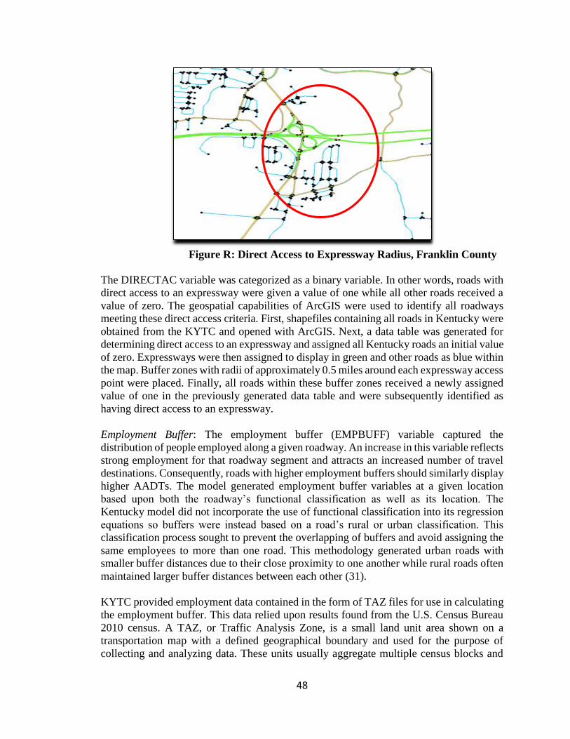
48

Figure R: Direct Access to Expressway Radius, Franklin County

The DIRECTAC variable was categorized as a binary variable. In other words, roads with

direct access to an expressway were given a value of one while all other roads received a

value of zero. The geospatial capabilities of ArcGIS were used to identify all roadways

meeting these direct access criteria. First, shapefiles containing all roads in Kentucky were

obtained from the KYTC and opened with ArcGIS. Next, a data table was generated for

determining direct access to an expressway and assigned all Kentucky roads an initial value

of zero. Expressways were then assigned to display in green and other roads as blue within

the map. Buffer zones with radii of approximately 0.5 miles around each expressway access

point were placed. Finally, all roads within these buffer zones received a newly assigned

value of one in the previously generated data table and were subsequently identified as

having direct access to an expressway.

Employment Buffer: The employment buffer (EMPBUFF) variable captured the

distribution of people employed along a given roadway. An increase in this variable reflects

strong employment for that roadway segment and attracts an increased number of travel

destinations. Consequently, roads with higher employment buffers should similarly display

higher AADTs. The model generated employment buffer variables at a given location

based upon both the roadway’s functional classification as well as its location. The

Kentucky model did not incorporate the use of functional classification into its regression

equations so buffers were instead based on a road’s rural or urban classification. This

classification process sought to prevent the overlapping of buffers and avoid assigning the

same employees to more than one road. This methodology generated urban roads with

smaller buffer distances due to their close proximity to one another while rural roads often

maintained larger buffer distances between each other (31).

KYTC provided employment data contained in the form of TAZ files for use in calculating

the employment buffer. This data relied upon results found from the U.S. Census Bureau

2010 census. A TAZ, or Traffic Analysis Zone, is a small land unit area shown on a

transportation map with a defined geographical boundary and used for the purpose of

collecting and analyzing data. These units usually aggregate multiple census blocks and

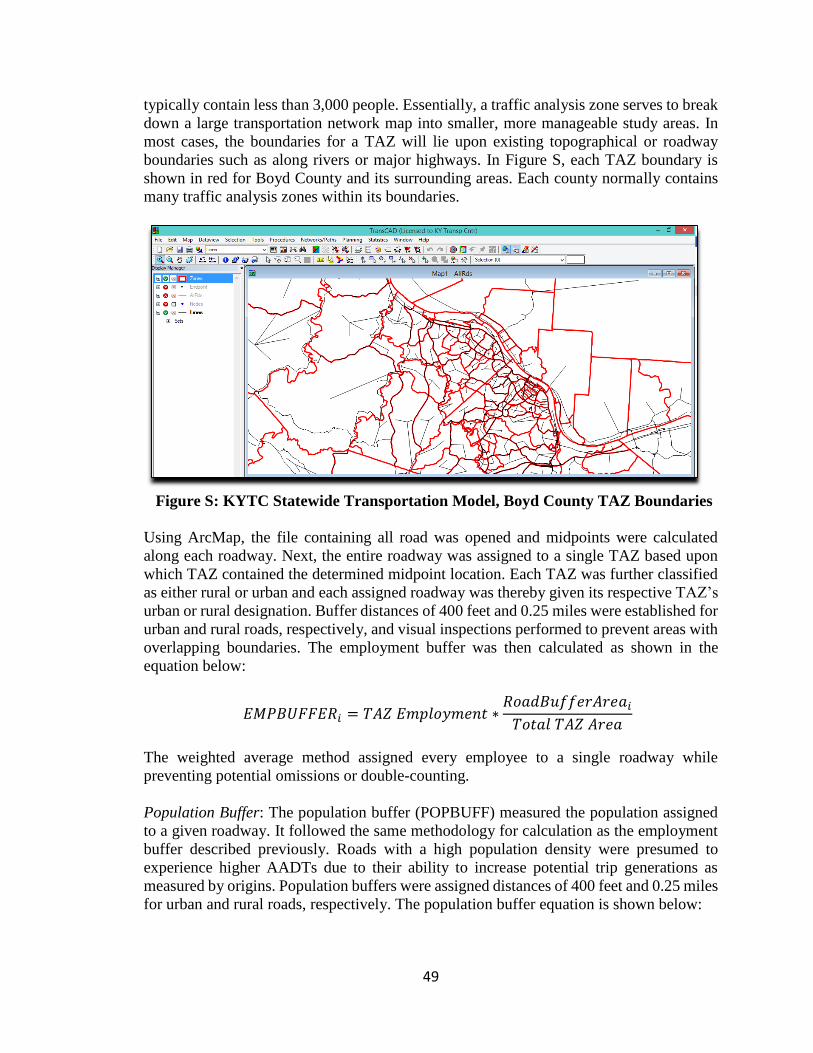
49

typically contain less than 3,000 people. Essentially, a traffic analysis zone serves to break

down a large transportation network map into smaller, more manageable study areas. In

most cases, the boundaries for a TAZ will lie upon existing topographical or roadway

boundaries such as along rivers or major highways. In Figure S, each TAZ boundary is

shown in red for Boyd County and its surrounding areas. Each county normally contains

many traffic analysis zones within its boundaries.

Figure S: KYTC Statewide Transportation Model, Boyd County TAZ Boundaries

Using ArcMap, the file containing all road was opened and midpoints were calculated

along each roadway. Next, the entire roadway was assigned to a single TAZ based upon

which TAZ contained the determined midpoint location. Each TAZ was further classified

as either rural or urban and each assigned roadway was thereby given its respective TAZ’s

urban or rural designation. Buffer distances of 400 feet and 0.25 miles were established for

urban and rural roads, respectively, and visual inspections performed to prevent areas with

overlapping boundaries. The employment buffer was then calculated as shown in the

equation below:

𝐸𝑀𝑃𝐵𝑈𝐹𝐹𝐸𝑅𝑖 = 𝑇𝐴𝑍 𝐸𝑚𝑝𝑙𝑜𝑦𝑚𝑒𝑛𝑡 ∗𝑅𝑜𝑎𝑑𝐵𝑢𝑓𝑓𝑒𝑟𝐴𝑟𝑒𝑎𝑖

𝑇𝑜𝑡𝑎𝑙 𝑇𝐴𝑍 𝐴𝑟𝑒𝑎

The weighted average method assigned every employee to a single roadway while

preventing potential omissions or double-counting.

Population Buffer: The population buffer (POPBUFF) measured the population assigned

to a given roadway. It followed the same methodology for calculation as the employment

buffer described previously. Roads with a high population density were presumed to

experience higher AADTs due to their ability to increase potential trip generations as

measured by origins. Population buffers were assigned distances of 400 feet and 0.25 miles

for urban and rural roads, respectively. The population buffer equation is shown below:

50

𝑃𝑂𝑃𝐵𝑈𝐹𝐹𝐸𝑅𝑖 = 𝑇𝐴𝑍 𝑃𝑜𝑝𝑢𝑙𝑎𝑡𝑖𝑜𝑛 ∗𝑅𝑜𝑎𝑑𝐵𝑢𝑓𝑓𝑒𝑟𝐴𝑟𝑒𝑎𝑖

𝑇𝑜𝑡𝑎𝑙 𝑇𝐴𝑍 𝐴𝑟𝑒𝑎

Distance to Population Center: The distance to the population center (DPOPCNTR)

measured the travel times from the centroid for an individual TAZ to the centroids of other

TAZs located in Kentucky. This variable considered each TAZ to be a population center.

The KYTC maintains a travel time matrix that provides travel times between the centroids

of every TAZ in the state. Using this approach, the defined centroid for each TAZ was used

as the spatial location of assignment for all roads within that TAZ and successively

calculated travel times between that select centroid and the centroid locations for all TAZs

across the state. This streamlined the calculation process by eliminating the need for

calculations between every roadway midpoint within the study area and all TAZ centroids

located across the state. This resulted in every roadway located within a select TAZ having

the same value for DPOPCNTR. However, most TAZs contained a minimal number of

roads (typically less than 25) so this proxy approach remained viable.

Regional Employment Access: The regional employment access (REACCESS) variable

accounted for trip distance and total employment at a given destination. The calculation

for determining this variable is seen below:

𝑅𝐸𝐴𝐶𝐶𝐸𝑆𝑆𝑘 = ∑ 𝐸𝑗 ∗ 𝑒−0.0954∗𝑡𝑘𝑗

𝑁𝐸

𝑗=1

Where

j is the TAZ centroid;

k is the TAZ that REACCESS is being calculated for

NE is the total number of TAZs

Ej is the total employment of TAZ j

tkj is the time from TAZ k to TAZ j

This model considered every TAZ to be a regional employment center. Similar to the

DPOPCNTR variable, this methodology determined travel times between centroids for

every respective TAZ within the state. In this equation, employment centers with

increased levels of employment coupled with short distances to roadways created a larger

trip distribution attraction and resulted in larger REACCESS values for those nearby

roadways. Finally, a query within Microsoft Access calculated REACCESS for every

single TAZ within Kentucky to produce the variables of interest.

Based upon these variables, a Kentucky model was developed using five of the original

Zhao and Chung model variables including: direct access to an expressway, employment

buffer, population buffer, distance to population center, and accessibility to regional

employment centers. The model drew upon obtained data from Boyd, Clark, Franklin,

Green, and Henry counties. The final regression equation used in this model was:

51

AADT = 357.23*DIRECTAC + 0.02*REACCESS – 0.63*POPBUFFER –

0.05*EMPBUFFER + 0.09*DISPOPCNTR

Using this regression equation, data were plotted to compare actual AADTs collected from

local traffic authorities to the estimated AADTs from the model. The results of this plot are

shown in Figure T.

Figure T: Broward County Model; Boyd, Clark, Franklin, Green, and

Henry Counties

In general, the estimative attributes of this model were limited. The large variation of data

scattered across the plot indicated excessive errors associated with this model. The errors

represented the deviations between AADTs the model estimated for a local roadway and

the actual AADTs known to occur based upon previously collected traffic counts. Each

distinctly colored line represents a different magnitude of error from the “true” value

represented by the black line within the middle portion of the graph. A 100 percent accurate

model would display all estimated data points along the black line so that the estimated

AADT would entirely match the actual AADT at any given traffic volume. Intuitively, no

model can achieve this degree of precision so the key is to optimize the model to the highest

performance possible. Following this framework, the red lines form an upper and lower

boundary showing a 100 percent error deviation between the estimated value and the actual

value. Correspondingly, an estimated AADT placed along the upper redline would be

exactly twice the value of the actual AADT. For example, an actual AADT of 600 intersects

the upper redline at an estimated AADT of 1200. In this context, errors provided a window

into the accuracy of the model to perform as intended and provide valid results. The

Broward County model graph remained limited in this regard due to the wide variation of

data spread across multiple error ranges (e.g., 100%, 200%, 300%).

0

200

400

600

800

1000

1200

0 200 400 600 800 1000 1200 1400 1600 1800 2000 2200

Mo

del

AA

DT

Actual AADT

Florida Model: Actual vs Predicted AADT (counts 2000 or less)

52

The results of this model’s regression function can be partly explained through the use of

the Broward County model itself. The state of Florida possesses unique transportation

attributes in relation to Kentucky. In particular, the majority of Florida’s local roadways

are urban in nature. This contrasts with Kentucky’s local roadways which tend to be rural

and occupied by lower traffic volumes. Due to these initial results and seemingly limited

applicability, it was decided to exclude the use of this particular model going forward. The

errors associated with this model and their descriptions are shown in Table 11.

Table 11: Broward County Model Errors

Measure of Effectiveness Broward County Model

MAPE (%) 125

Average Absolute Error 417

Maximum Positive Error (%) 833

Maximum Negative Error (%) -66

53

APPENDIX B: BROWARD COUNTY WITH PVA MODEL

This model version built upon select variables contained within the Zhao and Chung

Broward County model described in Appendix A and sought to enhance it by incorporating

property valuation administrator (PVA) data into the analysis. The most relevant variables

from the previously discussed Broward County model were extracted for use in this

enhanced model. The variables selected for inclusion were REACCESS, DISPOPCNTR,

POPBUFFER, and EMPBUFFER. To this extent, the variables DIRECTAC and LANES

were subsequently removed for use in this model due to lack of statistical significance.

Each of these two variables displayed little variation between different roadways within

the model thereby limiting their usefulness in estimating AADTs.

Next, PVA data was used as additional input into the regression model. Each county

government within Kentucky is responsible for determining and assessing taxes on its

residential and commercial properties. County governments perform these actions through

their internal or PVA office. In this effort, each PVA office collects and maintains data on

its jurisdictional properties including property owners, sizes, and addresses, among others.

The use of PVA data was sought as a tool to determine the number and type of properties

located along a local roadway.

The number of residential and commercial properties located adjacent to local roadways is

a determining factor for several AADT model variables such as trip generation and trip

distribution. Two of the county governments (Franklin and Meade) were contacted

requesting participation in this study in an effort to collect this information. The Franklin

County PVA provided use of their address database detailing the addresses of all

properties--both residential and commercial--known to exist along their local roads.

Furthermore, the Meade County road department also made their 911 emergency address

database available for use in this study. Similarly, this 911 database contained known

addresses for every residential or commercial property residing within its county borders.

This data—contained within the form of a shapefile—was merged using the route overlay

function in ArcMap and used to form the boundaries for each assessed property or parcel

of land in Franklin County. The Franklin County PVA classifies all of its properties into

one of 12 distinct categories. Within these categories, four were identified as displaying

the most utility to this model including RESIDENTIAL, COMMERCIAL,

AGRICULTURAL, and EDUCATIONAL. Each parcel was subsequently assigned to the

nearest roadway. The number of parcels assigned to each roadway was aggregated and

used this information in the follow-on regression analysis. The regression equation for this

model consisted of the following:

AADT = 4622.68 -0.01*REACCESS – 0.75*DISPOPCNTR + 0.35*POPBUFFER

– 0.92*EMPBUFFER – 0.56*RESIDENTIAL – 0.47*AGRICULTURAL +

17.92*COMMERCIAL – 3.81*EDUCATIONAL

This regression model represented incremental improvement over the previous and original

Broward County regression model. As can be seen below, the data more closely fit the

54

intended regression function as depicted by the black line located within the middle portion

of the graph (Figure U).

Figure U: Broward County with PVA Model, Franklin County

This model demonstrated improvement over the previous Broward County model across

three of the four error categories. The magnitude of the errors decreased for the MAPE,

average absolute error, and maximum positive error categories.

Table 12: Broward County with PVA Model Errors

Measure of Effectiveness Broward County with PVA

Model

MAPE (%) 82

Average Absolute Error 402



Nevertheless, the degree of improvement in relation to the original Broward County model

remained limited. Errors still occurred frequently across all three ranges of errors, or at the

100, 200, and 300 percent levels. To this extent, this model did not represent a significant

upgrade in estimating local road AADTs in relation to the original Broward County model.

Further study of the two remaining models was warranted.

0

200

400

600

800

1000

1200

1400

1600

1800

0 200 400 600 800 1000 1200 1400 1600 1800 2000

Mo

del

AA

DT

Actual AADT

Franklin County with Florida with PVA Actual vs Predicted AADT (counts 2000 or less)

55

APPENDIX C: ROOFTOP MODEL

In the “Rooftop” model, an aerial map in ArcMAP was used to visually determine the

number of properties through rooftop identification along local roadways. This approach

utilized Highway Information System data to populate roadway information within

ArcGIS. This approach was incorporated by visually identifying the number of rooftops

adjacent to roadways on this map using Google Earth. Each rooftop was thereby assigned

to the nearest roadway. In addition, rooftops were classified as small, medium, and large

and categorized according to the following attributes:

SMALL – Individual Houses

MEDIUM – Small Apartment Complex (e.g., Single Building), Minor

Buildings (e.g., small retail)

LARGE – Major Apartment Complex (e.g., Multiple Buildings), Major

Buildings (e.g., large retail), Industrial Complex or Facility

Next, a connectivity rating was established for roads within this “Rooftop” model by rating

roads from one to six based on their connectivity to other roads. The ranking system ranged

from a low rank assigned to dead end roads to the highest rank corresponding with urban

roads in a grid pattern. Visual inspection in ArcMap delineated the existence of dead end

roads. Mid-range rankings typically included the existence of minor collectors or major

through roads. It was possible to distinguish through roads and urban grid roads based on

the functional classifications found within the KYTC “All Roads” shapefile. The purpose

of the connectivity rating was to provide a variable that would account for the presence of

traffic on roadways that may not have any adjacent properties, thereby allowing the

regression model to have an intercept of zero.

The connectivity rating was used in conjunction with the three rooftop count variables to

run a regression for Meade County. The regression equation for this model was:

AADT = 113.8*CONNECTIVITY + 2.1*SMALL + 49.3*MEDIUM +

138.8*LARGE

Meade County data was used for this model in order to compare the results from this

regression analysis with that of the 911 model detailed in Appendix D. The 911 model only

used data from Meade County since 911 data had not been obtained from other Kentucky

counties. In general, the results from this model estimated higher than expected AADTs

for low-volume, local roads in comparison with actual traffic counts and lower than

expected AADTs for high-volume, local roads. The approximate range at which the

regression model moved from overestimating to underestimating actual AADTs occurred

around the 700 count threshold for the actual AADT. A graphic depicting the results from

this linear regression model is shown in Figure V.

56

Figure V: Rooftop Model, Meade County

The Rooftop model produced an increase in errors when compared to the previous Florida

with PVA model and therefore, did not improve upon the previous model. Furthermore,

this model represented the most time intensive methodology of the studied models. Due to

these reasons, it was decided to exclude this model for further analysis. The errors

associated with this model were as follows:

Table 13: Rooftop Model Errors

Measure of Effectiveness Rooftop Model

MAPE (%) 93

Absolute Error (AADT) 332



0

200

400

600

800

1000

1200

1400

1600

0 200 400 600 800 1000 1200 1400 1600

Esti

mat

e A

AD

T

Actual AADT

Meade County: Rooftop Model

57

APPENDIX D: 911 MODEL

The “911” model version utilized a similar approach to the PVA version by determining

residential and commercial property types through the use of 911 data. In this approach,

coordination with the Meade County Planning and Zoning Office was necessary for use of

their 911 database. This database contains listings of all known residential and commercial

properties within the county. Meade County provided this data in the form of a shapefile,

which can be used in ArcMap. This data was merged with the KYTC Highway Information

System (HIS) database. The HIS database is a KYTC maintained system containing the

elements of the roadway network such as roadway types, locations, and other attributes

across the state of Kentucky. The merging of this data allowed for the location of each 911

address and provided the ability to determine its proximity to nearby roadways. Properties

were subsequently assigned to the nearest roadway. Finally, the total number of properties

assigned to each roadway were aggregated and used in the follow-on regression analysis.

The regression equation for this model was:

AADT = 565.93 + 6.99*RESIDENTIAL+ 6.73*COMMERCIAL

However, this formula produced 565 vehicles per day on a road with no residential or

commercial properties alongside. Consequently, the regression was modified to force the

intercept to zero. The formula for this equation was as follows:

AADT = 43.5*RESIDENTIAL+ 16.4*COMMERCIAL

However, forcing the model to go through zero does not allow for accurate estimations of

through trips. Therefore, an intercept greater than zero, but less than the number estimated

by the regression may be more appropriate.

In this model, estimated AADTs tended to underestimate actual AADTs across much of

the traffic volume range from low to high traffic counts. The model results are shown

graphically in Figure W.

Figure W: 911 Model, Meade County

0

500

1000

1500

2000

2500

3000

0 500 1000 1500 2000 2500

Esti

mat

ed A

AD

T

Actual AADT

Meade County: 911 Model

58

The errors contained within this model are shown in the table below.

Table 14: 911 Model Errors

Measure of Effectiveness 911 Model

MAPE (%) 61

Absolute Error (AADT) 352



On average, the 911 model provided the best combination of results across the aggregated

error categories. It contained the lowest error values among all the models for the Mean

Absolute Percent Error (MAPE) and the Maximum Error as well as the second lowest

Absolute Error value. It happened to contain the highest minimum error value but this did

not differ significantly from the other model minimum error values. Aggregating the

overall errors, the 911 model was identified as the overall best performing model thus

warranting additional research efforts. However, it was later discovered that this data was

not accessible at the statewide level and therefore, this model was excluded for further

analysis.

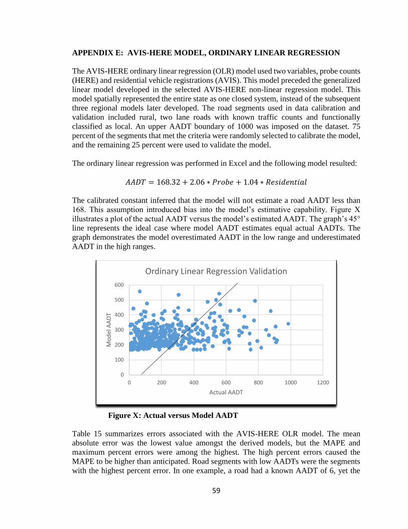
59

APPENDIX E: AVIS-HERE MODEL, ORDINARY LINEAR REGRESSION

The AVIS-HERE ordinary linear regression (OLR) model used two variables, probe counts

(HERE) and residential vehicle registrations (AVIS). This model preceded the generalized

linear model developed in the selected AVIS-HERE non-linear regression model. This

model spatially represented the entire state as one closed system, instead of the subsequent

three regional models later developed. The road segments used in data calibration and

validation included rural, two lane roads with known traffic counts and functionally

classified as local. An upper AADT boundary of 1000 was imposed on the dataset. 75

percent of the segments that met the criteria were randomly selected to calibrate the model,

and the remaining 25 percent were used to validate the model.

The ordinary linear regression was performed in Excel and the following model resulted:

𝐴𝐴𝐷𝑇 = 168.32 + 2.06 ∗ 𝑃𝑟𝑜𝑏𝑒 + 1.04 ∗ 𝑅𝑒𝑠𝑖𝑑𝑒𝑛𝑡𝑖𝑎𝑙

The calibrated constant inferred that the model will not estimate a road AADT less than

168. This assumption introduced bias into the model’s estimative capability. Figure X

illustrates a plot of the actual AADT versus the model’s estimated AADT. The graph’s 45°

line represents the ideal case where model AADT estimates equal actual AADTs. The

graph demonstrates the model overestimated AADT in the low range and underestimated

AADT in the high ranges.

Figure X: Actual versus Model AADT

Table 15 summarizes errors associated with the AVIS-HERE OLR model. The mean

absolute error was the lowest value amongst the derived models, but the MAPE and

maximum percent errors were among the highest. The high percent errors caused the

MAPE to be higher than anticipated. Road segments with low AADTs were the segments

with the highest percent error. In one example, a road had a known AADT of 6, yet the

0

100

200

300

400

500

600

0 200 400 600 800 1000 1200

Mo

del

AA

DT

Actual AADT

Ordinary Linear Regression Validation

60

model is estimated 168 based on the calibrated constant. This, in turn, created high errors.

Another method warranting additional investigation would be establishing a lower AADT

boundary on the calibration dataset and requiring exclusion for very low AADT road

segments.

Table 15: OLR Model Errors

Measure of Effectiveness OLR Model

N (sample size) 401

Mean Absolute Error 153

St. Dev. Absolute Error 124

MAPE (%) 192

Max % Error 5359

Min % Error -78

Table 16 summarizes errors for all studied models. On average, the 911 model provided

the best combination of results across the aggregated error categories. It contained the

lowest Mean Absolute Percent Error (MAPE) and Maximum Error values for all models

and the third lowest Absolute Error value. Its minimum error value exceeded other models

but not significantly. Aggregating the overall errors, the 911 model was identified as the

overall best performing model. However, the 911 data used to develop this model was not

readily available statewide. Therefore, the AVIS-HERE model was selected because it

demonstrated the best overall combination of performance and data availability due to its

low average absolute error.

Table 16: Summary of Model Errors

Measure of Effectiveness Florida Florida

with PVA Rooftop 911

AVIS-

HERE

OLR

MAPE (%) 125 82 93 61 192

Absolute Error (AADT) 417 402 332 352 153

Maximum Positive Error

(%)

833 399 494 190 5359

Maximum Negative Error

(%)

-66 -72 -60 -100 -78

61

REFERENCES

1 Federal Highway Administration (FHWA), Traffic Monitoring Guide, September 2013,

pg. 1-5 2 Pan, T. Assignment of estimated average annual daily traffic on all roads in Florida.In

Civil Engineering, No. Thesis, University of South Florida, 2008. p. 100. 3 Shen, L. D., F. Zhao, and D. I. Ospina. Estimation of Annual Average Daily Traffic for

Off-System Roads in Florida. In, 1999. p. 86 p. 4 Zhao, F., and S. Chung. Contributing Factors of Annual Average Daily Traffic in a

Florida County: Exploration with Geographic Information System and Regression

Models. Transportation Research Record, No. 1769, 2001, pp. p. 113-122. 5 Lowry, M., and M. Dixon. GIS Tools to Estimate Average Annual Daily Traffic.In,

2012. p. 33p. 6 Mohamad, D., K. Sinha, T. Kuczek, and C. Scholer. Annual Average Daily Traffic

Prediction Model for County Roads. Transportation Research Record: Journal of the

Transportation Research Board, Vol. 1617, No. -1, 1998, pp. 69-77. 7 Zhao, F., and N. Park. Using Geographically Weighted Regression Models to Estimate

Annual Average Daily Traffic. Transportation Research Record, No. 1879, 2004, pp. p.

99-107. 8 Selby, B., and K. Kockelman. Spatial Prediction of AADT in Unmeasured Locations by

Universal Kriging.In, 2011. p. 21p. 9 Eom, J. K., M. S. Park, T.-Y. Heo, and L. F. Huntsinger. Improving the Prediction of

Annual Average Daily Traffic for Nonfreeway Facilities by Applying a Spatial Statistical

Method. Transportation Research Record: Journal of the Transportation Research Board,

No. 1968, 2006, pp. pp 20-29. 10 Shamo, B., E. Asa, and J. Membah. Linear Spatial Interpolation and Analysis of

Annual Average Daily Traffic Data. Journal of Computing in Civil Engineering, Vol. 0,

No. 0, p. 04014022. 11 Wang, X., and K. M. Kockelman. Forecasting Network Data: Spatial Interpolation of

Traffic Counts from Texas Data. Transportation Research Record: Journal of the

Transportation Research Board, No. 2105, 2009, pp. pp 100-108. 12Sharma, S., P. Lingras, F. Xu, and P. Kilburn. Application of Neural Networks to

Estimate AADT on Low-Volume Roads. Journal of Transportation Engineering, Vol.

127, No. 5, 2001, pp. p. 426-432. 13Wang, T., A. Gan, and P. Alluri. Estimating Annual Average Daily Traffic for Local

Roads for Highway Safety Analysis. Transportation Research Record: Journal of the

Transportation Research Board, No. 2398, 2013, pp. pp 60–66. 14Wang, T. Improved Annual Average Daily Traffic (AADT) Estimation for Local Roads

using Parcel level Travel Demand Modeling.In, Florida International University, FIU

Electronic Theses and Dissertations, 2012. p. 135. 15Zhong, M., and B. L. Hanson. GIS-based travel demand modeling for estimating traffic

on low-class roads. Transportation Planning and Technology, Vol. 32, No. 5, 2009, pp.

423-439. 16Lowry, M. Spatial interpolation of traffic counts based on origin–destination centrality.

Journal of Transport Geography, Vol. 36, No. 0, 2014, pp. 98-105.

62

17Adler, T. J., Y. Dehghani, M. Doherty, and W. Olsen. Florida’s Turnpike State Model:

Development and Validation of an Integrated Land Use and Travel Forecasting Model.

TRB 86th Annual Meeting Compendium of Papers CD-ROM 2007. p. 14p. 18 Florida Department of Transportation. AADT Methodology for All Roads.

http://www2.dot.state.fl.us/trafficsafetywebportal/post/Post_332_Allocator%20Process.p

df. Accessed December 13, 2014. 19Arcgis Resource Center. How Kriging works.

http://help.arcgis.com/en/arcgisdesktop/10.0/help/index.html#//009z00000076000000.ht

m. Accessed on December 13, 2014. 20 Trip Generation Manual, Institute of Transportation Engineers (ITE). 9th edition.

http://www.ite.org/tripgeneration/trippubs.asp. Accessed on February 19, 2015. 21 National Highway Institute, Federal Highway Administration. Introduction to Travel

Demand Forecasting CD-ROM (FHWA-NHI-152054). Accessed on February 23, 2015 22 NAVMART. HERE Traffic Patterns. HERE. http://www.navmart.com/here-traffic-

patterns.php. Accessed June 18, 2015. 23 Jefferson County PVA. Motor Vehicle Assessment. Jefferson County Property

Valuation Assessment. https://jeffersonpva.ky.gov/property-assessment/motor-vehicle-

assessment. Accessed June 18, 2015. 24 Slash Gear. “Nokia HERE Research: We talk Smart Cities, ethical tracking & self-

driving cars”. http://www.slashgear.com/nokia-here-research-we-talk-smart-cities-

ethical-tracking-self-driving-cars-21294397/. Obtained on December 21, 2015. 25 ArcGIS Resource Center, Desktop 10.

http://help.arcgis.com/en/arcgisdesktop/10.0/help/index.html#//006600000001000000.

Accessed June 29, 2015 26 Kentucky Transportation Cabinet, Division of Planning. Highway Information System

GIS Extracts. http://transportation.ky.gov/Planning/Pages/HIS-Extracts.aspx. 27 Kentucky Transportation Cabinet, Division of Planning. Planning Highway

Information (HIS Database). Daily Vehicle Miles Traveled (DVMT) and Mileage

Reports. Accessed November 05, 2015. 28 U.S. Department of Transportation. Transportation for a New Generation Strategic

Plan, 2012-2016. Pg. 9 29 Federal Highway Administration (FHWA), Crash Cost Estimates by Maximum Police-

Reported Injury Severity within Selected Crash Geometries. FHWA-HRT-05-051.

October 2005. 30 American Association of State and Highway Transportation Officials (AASHTO).

Highway Safety Manual, 1st ed., Vol. 2. 2010. 31 Green, Eric R. and Agent, Kenneth R. Crash Rates at Intersections. Kentucky

Transportation Center, KTC-03-21/SPR258-03-2I. August 2003.

63

VITA

William Nicholas Staats, B.S, Graduate Research Assistant

Louisville, Kentucky

EDUCATION___________________________________________________________

BSCE University of Kentucky; Lexington, Kentucky. December 2014

2011 -2014 Bachelor of Science in Civil Engineering. GPA: 3.93

SERVICE AND PROFESSIONAL ACTIVITIES_____________________________

2016– Present Vice President, University of Kentucky Section of the Institute of

Transportation Engineers (UKITE).

2016 – Present Student member, Institute of Transportation Engineers (ITE).

2016 Member, UKITE Traffic Bowl Team.

2012 – Present Student member, American Railway Engineering and Maintenance-of-

Way Association (AREMA)

HONORS AND AWARDS_________________________________________________

2015 William Seymour Transportation Engineering Scholarship ($2,500),

sponsored by the Kentucky Section of the Institute of Transportation Engineers

2014 Oliver Raymond Scholarship ($2,500), sponsored by the College of

Engineering, University of Kentucky.

2014 Engineering Dean’s Circle Scholarship ($1,500), sponsored by the

College of Engineering, University of Kentucky.

2013 C. Michael Garver Scholarship ($2,500), sponsored by the College of

Engineering, University of Kentucky.

2011-2014 College of Engineering Dean's List, University of Kentucky

ESTIMATION OF ANNUAL AVERAGE DAILY TRAFFIC ON LOCAL …

Documents