Comparative Analysis of Traffic State Estimation ...eprints.qut.edu.au/90506/1/TRR2015_TT2_Accepted.pdf · Comparative Analysis of Traffic State Estimation ─ Cumulative Counts-based

Comparative Analysis of Traffic State Estimation ─ Cumulative Counts-based and Trajectory-based Methods

Takahiro Tsubota* Smart Transport Research Centre Science and Engineering Faculty Queensland University of Technology 2 George St. GPO Box 2434, Brisbane QLD 4001, Australia Phone: +61 7 3138 9994 e-mail: [email protected] Ashish Bhaskar Smart Transport Research Centre Science and Engineering Faculty Queensland University of Technology 2 George St. GPO Box 2434, Brisbane QLD 4001, Australia Phone: +61 7 3138 9985 e-mail: [email protected] Alfredo Nantes Smart Transport Research Centre Science and Engineering Faculty Queensland University of Technology 2 George St. GPO Box 2434, Brisbane QLD 4001, Australia Phone: +61 7 3138 9985 e-mail: [email protected] Edward Chung Smart Transport Research Centre Science and Engineering Faculty Queensland University of Technology 2 George St. GPO Box 2434, Brisbane QLD 4001, Australia Phone: +61 7 3138 1143 e-mail: [email protected] Vikash V. Gayah Department of Civil and Environmental Engineering The Pennsylvania State University 231L Sackett Building, University Park, PA 16802 Phone: 814 865 4014 e-mail: [email protected] *Corresponding author 5,445 words + 8 figures = 7,445 words Submitted and accepted for publication in Transportation Research Record: Journal of the Transportation Research Board

mailto:[email protected]





1 Tsubota, Bhaskar, Nantes, Chung, Gayah

ABSTRACT 1

The Macroscopic Fundamental Diagram (MFD) relates space-mean density and flow. Since the 2 MFD represents the area-wide network traffic performance, studies on perimeter control 3 strategies and network-wide traffic state estimation utilising the MFD concept has been reported. 4 Most previous works have utilised data from fixed sensors, such as inductive loops, to estimate 5 the MFD, which can cause biased estimation in urban networks due to queue spillovers at 6 intersections. To overcome the limitation, recent literature reports the use of trajectory data 7 obtained from probe vehicles. However, these studies have been conducted using simulated 8 datasets; limited works have discussed the limitations of real datasets and their impact on the 9 variable estimation. 10

This study compares two methods for estimating traffic state variables of signalised 11 arterial sections: a method based on cumulative vehicle counts (CUPRITE), and one based on 12 vehicles’ trajectory from taxi GPS log. The comparisons reveal some characteristics of taxi 13 trajectory data available in Brisbane, Australia. The current trajectory data has limitations in 14 quantity (i.e., the penetration rate), due to which the traffic state variables tend to be 15 underestimated. Nevertheless, the trajectory-based method successfully captures the features of 16 traffic states, which suggests that the trajectories from taxis can be a good estimator for the 17 network-wide traffic states. 18 19 20 21


INTRODUCTION 1

For decades, aggregate traffic behaviour in large urban areas has been observed and modelled 2 based on the empirical observations (1-3) and the two-fluid model (4). Recently, Daganzo (5) 3 reinitiated modelling network-wide traffic states to describe urban gridlock phenomena, which 4 was later verified by Geroliminis and Daganzo (6) using loop detectors and probe vehicles’ data 5 from downtown Yokohama, Japan. The relation, termed as “Network Fundamental Diagram” 6 (NFD) or “Macroscopic Fundamental Diagram” (MFD), represents an area traffic states by 7 defining the traffic throughput of an area at given density levels, and describes the dynamics of 8 area-wide traffic conditions. In recent years, the properties of the MFD have been intensively 9 investigated (7-16) for properly implementing the concept for traffic control strategies (17-25). 10

Most previous works have relied on the measurements from fixed sensors, such as 11 inductive loop detectors, from either simulated or real world networks. However, the variable 12 estimation from these sensors is challenging in signalised urban networks. Unlike freeway 13 networks, signalised arterials are characterised by stop-and-go behaviours, and the density from 14 the point measurement cannot represent the traffic states of the whole section. The occupancy (or 15 the density) from the stop line detectors is highly biased due to the stopping vehicles during red 16 time phases, as reported in literatures (26; 27). In fact, Courbon and Leclercq (28) demonstrated 17 that the shape of the MFD is highly influenced by the locations of detectors (in terms of the 18 distance from the stop line) employed for density estimations. 19

Alternatively, Tsubota, et al. (29) fused loop counts with probe samples (i.e., Bluetooth 20 data) to estimate unbiased section density, based on CUPRITE model (30; 31). After validating 21 the accuracy in a simulation (32), they applied the method to estimate the MFD from signalised 22 urban network of Brisbane, Australia (33). However, the studied network is limited to the 23 particular subset equipped with Bluetooth scanners; it only covered major arterials excluding 24 minor roads and side streets. 25 With the growing availability of GPS data from mobile sensors, the use of their 26 trajectories has become of interest for researchers to estimate network-wide traffic states and the 27 MFD. Unlike the Bluetooth data, the GPS data from probes cover a wider range of the network 28 including minor streets. Moreover, it can provide detailed trajectories of individual vehicles 29 throughout a section. Therefore, if sufficient sample is available, vehicle trajectories can provide 30 a more reliable estimator of the network traffic states as demonstrated in recent works(33-35). 31 However, these evaluations are conducted in simulation environments, which lack many real-32 world complexities. The investigation on the limitations of the currently available data (e.g., taxi 33 GPS) is still missing, such as the impact of their actual penetration rate and spatial distribution to 34 the variable estimation, which hinders the reliable introduction of the trajectory-based data to the 35 real-world control strategies. 36 To address the issue, this study compares the MFDs from two different methods: the 37 CUPRITE-based method that fuses loop counts with Bluetooth data (33), and the trajectory-38 based method using taxi GPS log, available from a major corridor in Brisbane, Australia. Both 39 methods estimate the MFD of the same corridor to discuss the limitations of the current taxi 40 sample, and to identify the future research directions. 41 42

43

44


STUDY SITE AND DATA DESCRIPTIONS 1

Study site – a major corridor 2

Figure 1 shows a major corridor of Brisbane: Coronation Drive (inbound towards Central 3 Business District (CBD)). Length of the section is 4.2 km, with three lanes in each direction. 4 Bluetooth Media Access Control Scanners (BMS scanners) are located at major signalised 5 intersections, highlighted with yellow ‘pins’ in Figure 1. Since this study focus on a corridor, not 6 a network, the estimated diagrams will be Arterial Fundamental Diagram (AFD) or Arterial 7 MFD. 8

Stop Line Detector and Signal Phase Data 9

The signal controls in Brisbane surface streets are equipped with Sydney Coordinated Adaptive 10 Traffic System (SCATS). The signalised intersections are centrally controlled and the data from 11 the controller is stored by Brisbane City Council. The detector counts and signal phases for this 12 study are collected from the SCATS traffic reporter and history reader. The vehicle counts are 13 measured at stop lines for each lane and aggregated every five minutes. 14

Bluetooth Records as Probe Vehicle Samples 15

BMS scanners (36) are increasingly used for travel time estimation and prediction (37), and are 16 identified to be a good source of probe for CUPRITE. BMS scanners have been installed at 17 major intersections by Brisbane City Council for traffic monitoring purposes. A BMS scanner 18 has a particular range of communication termed as coverage area (e.g. 100 meter radius), within 19 which it detects Bluetooth equipped electronic devices such as mobile phones, laptops and in-20 build Bluetooth in cars, and records their Media Access Control (MAC) ID and corresponding 21 timestamp. MAC ID is a unique anonymous identifier allocated to each device. By matching 22 MAC IDs at two different locations, the travel time can be calculated as the difference of the 23 timestamps. If vehicles with active Bluetooth device are recorded at two successive intersections, 24 the difference of the upstream and downstream passing time gives the individual vehicles’ travel 25 time. Interested readers should refer to Bhaskar and Chung (38) for details on the use of BMS 26 scanners as complementary transport data. For CUPRITE application, we are only interested in 27 the time when the probe is at upstream and downstream locations. Thus, the Bluetooth record is 28 a good proxy for probe required by CUPRITE model. 29 Bluetooth data includes various transportation modes, such as pedestrians and bicycles 30 (39). Although the sample size of such data is relatively small, this causes significant scatters in 31 Bluetooth travel time profile. The Median Absolute Deviation technique is applied for removing 32 outliers in travel time profile. The method defines Upper Bound and Lower Bound Values (UBV 33 and LBV, respectively) from sample median and the median absolute deviation from the median 34 (37). The samples larger than the UBV or smaller than LBV are considered as outliers. 35 𝑈𝑈𝑈𝑈𝑈𝑈 = 𝑚𝑚𝑚𝑚𝑚𝑚𝑚𝑚𝑚𝑚𝑚𝑚 + 𝜎𝜎𝜎𝜎 (1)

𝐿𝐿𝑈𝑈𝑈𝑈 = 𝑚𝑚𝑚𝑚𝑚𝑚𝑚𝑚𝑚𝑚𝑚𝑚 − 𝜎𝜎𝜎𝜎 (2)

Where 𝜎𝜎 is the standard deviation from the MAD, which is approximated as 𝜎𝜎 = 1.4826 × 𝑀𝑀𝑀𝑀𝑀𝑀, 36 assuming the data being normally distributed. MAD is defined as 37 𝑀𝑀𝑀𝑀𝑀𝑀 = 𝑚𝑚𝑚𝑚𝑚𝑚𝑚𝑚𝑚𝑚𝑚𝑚(�𝑋𝑋𝑖𝑖 − 𝑚𝑚𝑚𝑚𝑚𝑚𝑚𝑚𝑚𝑚𝑚𝑚(𝑋𝑋𝑗𝑗)�). (3)

4 Tsubota, Bhaskar, Nantes, Chung, Gayah The value of 𝜎𝜎𝜎𝜎 defines the scatter of the sample. The parameter 𝜎𝜎 is a scale factor that 1 determines the gap between UBV and LBV. For this study, 𝜎𝜎 = 2 is chosen as suggested in Kieu, 2 et al. (39). 3

Overview of taxi data 4

Taxi GPS log provides trajectories of individual vehicles. The behaviour of taxis is not identical 5 to normal vehicles because they follow circuitous routes to search for passengers; wait in a queue 6 at taxi ranks; and, stop more frequently to pick up passengers. These unique behaviours are 7 typically observed only when they are empty; once carrying a passenger, the taxi can be assumed 8 to behave as if they were an ordinary car. 9 The taxi data provides “timestamp”, “geolocation (longitude and latitude)”, “vehicle 10 speed”, “driving direction (anticlockwise angle from the horizontal axis (i.e., latitude lines))” and 11 the “states” of the taxi. The states include: 12

• “Meter On” (state 1) indicating the taxi is carrying passengers, 13 • “Logged On” (state 2) indicating the taxi is empty, and 14 • “Ignition On” (state 3) and “Ignition Off” (state 4) indicating the taxi starts and stops the 15

engine, respectively. 16

This study uses only the passenger-carrying taxis (state 1) as an estimator of the corridor 17 traffic states. The corridor MFD, the relation between flow and density of all vehicles, is 18 estimated by scaling up the flow and density of the taxi samples. The detailed process is 19 provided later in this paper. 20

STATE ESTIMATION BASED ON CUMULATIVE COUNTS – CUPRITE 21

Architecture of CUPRITE 22

CUPRITE integrates probe vehicle samples with cumulative plots U(t) and D(t) defined at the 23 upstream and downstream of the section, respectively. By introducing probe samples that 24 traverse the whole section, the cumulative plots are modified and the drifting of the plots due to 25 counting errors and/or mid-link sinks (see below) and sources can be reduced or cancelled. This 26 method draws reliable cumulative plots at upstream and downstream intersections; the vertical 27 distance of the plots represents the number of vehicles in the section, thus the density of the 28 section. 29 Here, probe vehicles are the vehicles equipped with vehicle tracking equipment. We 30 assume that the timestamps of a probe vehicle at upstream (𝑡𝑡𝑢𝑢) and downstream (𝑡𝑡𝑑𝑑) locations 31 are accurately obtained. The travel time of this vehicle is 𝑡𝑡𝑑𝑑 − 𝑡𝑡𝑢𝑢. We define the rank of the 32 probe vehicle in the cumulative plots as 𝑀𝑀(𝑡𝑡𝑑𝑑), given that the section is equipped with stop line 33 detectors and the downstream counts are more reliable than upstream ones. Thus, we fix probe’s 34 rank with 𝑀𝑀(𝑡𝑡) and define the points through which upstream plots 𝑈𝑈(𝑡𝑡) should pass. 35 Figure 2 summarises the CUPRITE architecture for density estimation assuming a mid-36 link sink case, where upstream detector is overcounting (for detail, refer to Bhaskar, et al.(31)). 37 Step 1: Cumulative plots are defined with upstream and downstream detector counts and signal 38 phase data. 39 Step 2: Probe data (the list of ([𝑡𝑡𝑢𝑢] and [𝑡𝑡𝑑𝑑]) is fixed with downstream cumulative plots and the 40 rank for each probe vehicle is defined [𝑀𝑀(𝑡𝑡𝑑𝑑)]. 41 Step 3: Points through which 𝑈𝑈(𝑡𝑡) should pass are defined from the list of [𝑡𝑡𝑢𝑢] and [𝑀𝑀(𝑡𝑡𝑑𝑑)]. 42

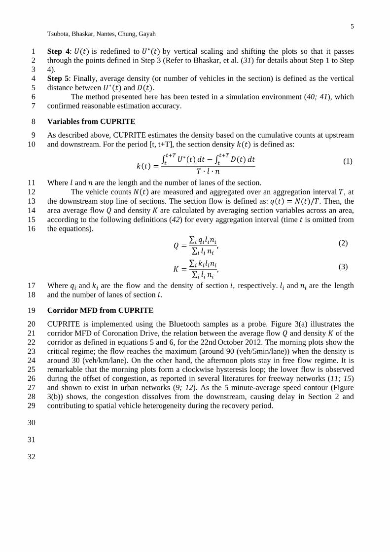
5 Tsubota, Bhaskar, Nantes, Chung, Gayah Step 4: 𝑈𝑈(𝑡𝑡) is redefined to 𝑈𝑈∗(𝑡𝑡) by vertical scaling and shifting the plots so that it passes 1 through the points defined in Step 3 (Refer to Bhaskar, et al. (31) for details about Step 1 to Step 2 4). 3 Step 5: Finally, average density (or number of vehicles in the section) is defined as the vertical 4 distance between 𝑈𝑈∗(𝑡𝑡) and 𝑀𝑀(𝑡𝑡). 5

The method presented here has been tested in a simulation environment (40; 41), which 6 confirmed reasonable estimation accuracy. 7

Variables from CUPRITE 8

As described above, CUPRITE estimates the density based on the cumulative counts at upstream 9 and downstream. For the period [t, t+T], the section density 𝑘𝑘(𝑡𝑡) is defined as: 10

𝑘𝑘(𝑡𝑡) =∫ 𝑈𝑈∗(𝑡𝑡)𝑡𝑡+𝑇𝑇𝑡𝑡 𝑚𝑚𝑡𝑡 − ∫ 𝑀𝑀(𝑡𝑡)𝑡𝑡+𝑇𝑇

𝑡𝑡 𝑚𝑚𝑡𝑡𝑇𝑇 ∙ 𝑙𝑙 ∙ 𝑚𝑚

(1)

Where 𝑙𝑙 and 𝑚𝑚 are the length and the number of lanes of the section. 11 The vehicle counts 𝑁𝑁(𝑡𝑡) are measured and aggregated over an aggregation interval 𝑇𝑇, at 12 the downstream stop line of sections. The section flow is defined as: 𝑞𝑞(𝑡𝑡) = 𝑁𝑁(𝑡𝑡)/𝑇𝑇. Then, the 13 area average flow 𝑄𝑄 and density 𝐾𝐾 are calculated by averaging section variables across an area, 14 according to the following definitions (42) for every aggregation interval (time 𝑡𝑡 is omitted from 15 the equations). 16

𝑄𝑄 =∑ 𝑞𝑞𝑖𝑖𝑙𝑙𝑖𝑖𝑚𝑚𝑖𝑖𝑖𝑖∑ 𝑙𝑙𝑖𝑖𝑖𝑖 𝑚𝑚𝑖𝑖

, (2)

𝐾𝐾 =∑ 𝑘𝑘𝑖𝑖𝑙𝑙𝑖𝑖𝑚𝑚𝑖𝑖𝑖𝑖∑ 𝑙𝑙𝑖𝑖𝑖𝑖 𝑚𝑚𝑖𝑖

, (3)

Where 𝑞𝑞𝑖𝑖 and 𝑘𝑘𝑖𝑖 are the flow and the density of section 𝑚𝑚, respectively. 𝑙𝑙𝑖𝑖 and 𝑚𝑚𝑖𝑖 are the length 17 and the number of lanes of section 𝑚𝑚. 18

Corridor MFD from CUPRITE 19

CUPRITE is implemented using the Bluetooth samples as a probe. Figure 3(a) illustrates the 20 corridor MFD of Coronation Drive, the relation between the average flow 𝑄𝑄 and density 𝐾𝐾 of the 21 corridor as defined in equations 5 and 6, for the 22nd October 2012. The morning plots show the 22 critical regime; the flow reaches the maximum (around 90 (veh/5min/lane)) when the density is 23 around 30 (veh/km/lane). On the other hand, the afternoon plots stay in free flow regime. It is 24 remarkable that the morning plots form a clockwise hysteresis loop; the lower flow is observed 25 during the offset of congestion, as reported in several literatures for freeway networks (11; 15) 26 and shown to exist in urban networks (9; 12). As the 5 minute-average speed contour (Figure 27 3(b)) shows, the congestion dissolves from the downstream, causing delay in Section 2 and 28 contributing to spatial vehicle heterogeneity during the recovery period. 29

30

31

32


TRAJECTORY-BASED STATE ESTIMATION 1

Data cleansing – map matching and trip extraction 2

A taxi works as a sensor moving in a network, and reports their locations in the space (geo-3 locations) and the timestamps every uplink intervals (i.e., 30 seconds), with which their 4 trajectories are reconstructed. Unlike the measurements by local observations, such as loop 5 detectors, this data provides the information about the spatial and temporal aspects of the traffic 6 conditions experienced by the vehicles. 7

The taxi GPS log provides whole trajectories of taxis within a day. Before estimating 8 traffic states, the data required cleaning to extract trips along the study site (i.e., Coronation 9 Drive) from the continuous trajectories. This study employs the following steps to determine the 10 trips along the study site: 11 Step 1: Data extraction along the study site 12 Step 2: Extraction of passenger-carrying taxis based on “States” 13 Step 3: Identification of trip ends 14 Step 4: Identification of U-turns 15 16 Step 1: The GPS plots along the study site are extracted based on their distances from the nearest 17 section and their driving directions. A 10-metre buffer zone is defined along the corridor, and 18 any plots outside the buffer are removed from the analysis. Vehicles are expected to be driving 19 along the road and ideally, the driving direction from GPS should match with the direction of the 20 road section defined from upstream node to the downstream node. Therefore, for the remaining 21 plots, the relative angle (θ1), defined as the absolute difference of the driving direction and the 22 section direction is estimated. If the relative angle exceeds 20 degree, the plots are removed. 23 Figure 4 (a) illustrates data extraction in step 1. 24 Step 2: This study uses passenger-carrying taxis as a proximity of ordinary cars. The taxi GPS 25 log includes the “State” as explained in the overview of taxi data. In this step, the data only the 26 logs with “Meter On” (State 1) are extracted and used for the further analysis. 27 Step 3: The GPS log is recorded every uplink interval (i.e., 30 seconds). However, longer time 28 gaps can occur due to communication errors, states being switched from “Meter On” to others 29 (e.g., “Logged On”), and/or the taxi driving into side streets and coming back to the study site. 30 When a gap is small, say a few minutes, and the vehicle changes locations during the gap, it 31 would be safe to bridge the gap by connecting the points before and after the gap, assuming the 32 gap is due to communication errors and the trip continues. However, when a gap is larger, say 33 over 10 minutes, other events could occur during this time, such as the taxi dropping off and 34 picking up passengers and the taxi driving outside the study site. In this study, 10 minutes (600 35 seconds) is used as a threshold to determine the gap ending the trip, based on the actual 36 frequency of gaps (Figure 4 (b)). Nearly 84% of gaps are within three minutes (180 seconds). 37 The other 16% range from 10 minutes to a few hours or over, which clearly separate trips. In the 38 other investigation (43), 15 minutes is recommended as a threshold, which aligns with ours. 39 Step 4: Finally, the shape of the trajectory is checked to exclude U-turns because the study 40 section is one-directional single corridor; taxis should always move from upstream to 41 downstream without any loops. The shape is checked using consecutive two plots in a trip and 42 their driving direction (Figure 4 (c)). If the angle of the current driving direction at time t, 43 θ2, with respect to the next position at time t+1 exceeds a threshold value, the taxi is assumed to 44

7 Tsubota, Bhaskar, Nantes, Chung, Gayah take a U-turn, and the plot at time t is assumed to be the end of the trip. Considering the shape of 1 the corridor, 90 degree is used as the threshold. 2

Trip distribution in space 3

The distribution of taxi trips may not be spatially homogeneous – more taxis can be observed 4 closer to the CBD area. If the proportion of the taxis to the full traffic is same (or similar) 5 throughout the corridor, the trajectories of taxis equally represent the traffic states at any sections 6 of the corridor, thus the corridor can be treated as a whole; otherwise the traffic states must be 7 estimated section by section considering the penetration rate of taxis in each section. 8 Figure 5 summarises the spatial distribution of taxi trips. The horizontal axis (x-axis) 9 shows the starting location of a trip expressed as the distance from the entrance of the corridor. 10 The vertical axis (y-axis) is the trip distance along the corridor. All the trips are mapped onto the 11 diagram inside the triangular area bounded with the hypotenuse line defined as y=L-x, where L is 12 the corridor length (left hand side of Figure 5). For instance, a taxi, which enters at the entrance 13 (x=0) and travels 4,000 metres along the corridor (y=4,000), is plotted at (0, 4000). Regardless of 14 the entering locations (x), all the trips travelling towards the end of the corridor will be plotted 15 onto the hypotenuse line because their trip lengths are expressed as L-x. 16 The contour on the right hand side of Figure 5 shows the frequency of the trips. Most 17 plots are mapped along the hypotenuse line, indicating most taxis travelling towards the end; 18 entering into the CBD area. However, the trip distribution is not uniform over the space. The 19 figure also indicates the locations of major side streets. One can recognise slightly denser plots 20 when side streets connect with Coronation Drive. Note also that blanks are located where there is 21 no side street (see the dotted rectangular in Figure 5). The highest proportion of trips is observed 22 around x=3,500 (circled in red), where another major road, Inner City Bypass, merges with 23 Coronation Drive. This observation confirms that the taxi trajectories do not equally represent 24 over the corridor. Therefore, the traffic states have to be estimated section by section, as 25 presented in Figure 1. 26

Estimation of the corridor MFD based on Edie’s definition 27

The generalised definitions of traffic flow variables, such as flow and density, were originally 28 introduced by Edie (42) based on the two-dimensional diagram as presented in Figure 6 to 29 describe traffic states of a single corridor. These consider the full behaviours of individual 30 vehicles in time and space, and should provide accurate estimates if enough trajectory data is 31 used to inform them. Recent advancement in new measurement techniques has enabled obtaining 32 trajectories from more vehicles. Consequently, the traffic state estimation utilising such 33 measurement has become of interest to researchers (27; 34; 35). An extended form of Edie’s 34 definitions has been proposed by Saberi, et al. (27) to describe traffic states of a network, based 35 on three-dimensional time-space diagram, not only of a corridor. However, our study focuses on 36 a corridor (Figure 1), thus original definitions by Edie (42) is employed. 37

The traffic states are estimated section by section using taxi trajectory data. The sections 38 are defined as consecutive two yellow pins along Coronation Drive in Figure 1. Let us consider a 39 rectangular region in time and space with dimensions of T and l, respectively as presented in 40 Figure 6. According to Edie (42), the variables, flow and density, are defined based on Total 41 Distance Travelled and Total Time Spent by taxi (TDTT and TTST, respectively) as defined below, 42 for section i. 43


𝑇𝑇𝑀𝑀𝑇𝑇𝑖𝑖𝑇𝑇 = �𝑚𝑚𝑖𝑖,𝑘𝑘𝑘𝑘

(1)

𝑇𝑇𝑇𝑇𝑇𝑇𝑖𝑖𝑇𝑇 = �𝑟𝑟𝑖𝑖,𝑘𝑘𝑘𝑘

(2)

Where 𝑚𝑚𝑖𝑖,𝑘𝑘 and 𝑟𝑟𝑖𝑖,𝑘𝑘 denote the distance travelled and time spent by vehicle 𝑘𝑘 in section 𝑚𝑚 , 1 respectively during a time period T. The 𝑚𝑚𝑖𝑖,𝑘𝑘 and 𝑟𝑟𝑖𝑖,𝑘𝑘 are derived from two consecutive reports of 2 the taxi GPS. When they happen on different sections, the time and distance between the 3 consecutive reports are decomposed to each section in proportion to the section length between 4 the two reports. Then, the flow and density of taxi samples are defined as: 5

𝑞𝑞𝑖𝑖𝑇𝑇 = 𝑇𝑇𝑀𝑀𝑇𝑇𝑖𝑖𝑇𝑇/(𝑚𝑚𝑖𝑖 ∙ 𝑙𝑙𝑖𝑖 ∙ 𝑇𝑇) (3)

𝑘𝑘𝑖𝑖𝑇𝑇 = 𝑇𝑇𝑇𝑇𝑇𝑇𝑖𝑖𝑇𝑇/(𝑚𝑚𝑖𝑖 ∙ 𝑙𝑙𝑖𝑖 ∙ 𝑇𝑇) (4)

Where 𝑞𝑞𝑖𝑖𝑇𝑇 and 𝑘𝑘𝑖𝑖𝑇𝑇 denote the flow and density of taxi samples in section 𝑚𝑚 . 𝑚𝑚𝑖𝑖 and 𝑙𝑙𝑖𝑖 are the 6 number of lanes and the length of section 𝑚𝑚. 𝑇𝑇 is the aggregation interval. Then, the flow (𝑞𝑞𝑖𝑖) and 7 density (𝑘𝑘𝑖𝑖) of full traffic is estimated as: 8

𝑞𝑞𝑖𝑖 = 𝑞𝑞𝑖𝑖𝑇𝑇/𝑋𝑋𝑖𝑖 (5)

𝑘𝑘𝑖𝑖 = 𝑘𝑘𝑖𝑖𝑇𝑇/𝑋𝑋𝑖𝑖 (6)

Where 𝑋𝑋𝑖𝑖 is the proportion of the number of taxi 𝑁𝑁𝑖𝑖𝑇𝑇 to full traffic counts 𝑁𝑁𝑖𝑖 in section 𝑚𝑚 , 9 calculated for every aggregation interval. Finally, the area average flow 𝑄𝑄 and density 𝐾𝐾 are 10 calculated as defined by equations 5 and 6. 11

RESULTS – COMPARISON OF CORRIDOR MFDS 12

Figure 7 (a) shows the corridor MFD from taxi trajectory data. The graph on the right presents 13 the closer look at the red square in the left graph. The morning plots show that the flow reaches 14 the maximum (around 70 (veh/5min/lane)) when the density is around 25 (veh/km/lane), whereas 15 the afternoon plots stay in free flow regime. The plots also exhibit hysteresis-like loops during 16 the morning peak, as observed in the corridor MFD estimated using CUPRITE (Figure 3). 17 However, the flow and density estimated from the taxi data are smaller than the one from 18 CUPRITE. Figure 7 (b) compares the corridor MFDs from two methods, the one from CUPRITE 19 (Figure 3) and the other from taxi data (Figure 7 (a)), together with the parabolic approximations 20 of the plots. As well, Figure 7 (c) compares the time-series of variables (density and flow) from 21 the different methods. As the figures show, the variables estimated from taxi trajectories are 22 smaller, only about two-thirds of the values estimated from CUPRITE. 23

This is because the taxi samples do not always represent the traffic states of the whole 24 corridor. Figure 8 (a) summarises the penetration of taxi samples for section 4, for example, 25 during morning peak (from 6AM to 11AM). The penetration rate is very low, below 3% for most 26 of the time. Moreover, there are instances when no taxi sample is available in one or more 27 sections, during which traffic states cannot be estimated. 28

9 Tsubota, Bhaskar, Nantes, Chung, Gayah Another issue in using taxi data is found by checking their average trip length (𝑇𝑇𝑀𝑀𝑇𝑇𝑖𝑖𝑇𝑇/1 𝑁𝑁𝑖𝑖𝑇𝑇). Figure 8 (b) shows the average trip length of taxi samples in section 4 during the morning 2 peak. The section is about 360 metres long, which is indicated with red line in the figure. 3 However, the average trip length of taxies is shorter in many instances, which implies that the 4 taxi samples represent only fractions of the study area. Due to this, the variables based on taxi 5 trajectories are mostly underestimated. On the contrary, CUPRITE employs Bluetooth samples 6 that traverse the whole sections, and thus it considers the section-wide traffic conditions. 7

DISCUSSIONS AND CONCLUSIONS 8

This study discovers interesting characteristics of the real taxi trajectory data available in 9 Brisbane, Australia. Firstly, the taxi samples are not uniformly distributed across the corridor; 10 rather they represent more in downstream sections. In such case, trajectory-based estimation may 11 be biased unless the corridor (or network) is properly separated considering the proportion of 12 taxis. Moreover, the trajectory-based method highly underestimates the variables compared with 13 the CUPRITE-based method. This can be because the penetration rate of taxi sample is still very 14 low (<3% during peak hours); only a fraction of their trajectories are available in most estimation 15 intervals, which causes underestimation of total time spent (TTS) and total distance travelled 16 (TDT) by taxi samples. 17 Nevertheless, the trajectory-based method successfully captures the features of traffic 18 states, such as peaks and off-peaks of density and flow, and the hysteresis loops in the MFD. It 19 should also be noted that the MFD from the trajectory-based method successfully represents the 20 critical density and the congestion regime, which are vital for traffic control purposes. These 21 findings confirm the usefulness of the taxi trajectories as an estimator of the network-wide traffic 22 states; and the possibility of area traffic control relying on the trajectory-based data sources. As 23 recognised by Nagle and Gayah (35), the more probe samples are available, the more confidence 24 one can have in estimated traffic states. Furthermore, higher uplink frequency (e.g., a few 25 seconds) may provide better estimation of variables. The future research needs include the 26 validation of the findings in controlled environments. The observation and discussion based on 27 the real data set also encourage further development of control strategies based on the trajectory 28 data. 29

ACKNOWLEDGEMENT 30

The authors would like to acknowledge Brisbane City Council and Black & White Cabs for 31 providing valuable data for this research. 32

REFERENCES 33

[1] Smeed, R. J. The Road Capacity of City Centres. Highway Research Record, Vol. No 169, 34 1966, pp. 22-29. 35 [2] Wardrop, J. G. Journey Speed and Flow in Central Urban Areas. Traffic Engineering & 36 Control, Vol. Volume: 9 No. Issue Number: 11, 1968. 37 [3] Godfrey, J. W. The Mechanism of a Road Network. Traffic Engineering and Control, Vol. 38 11, No. 7, 1969, pp. 323-327. 39 [4] Mahmassani, H. S., J. C. Williams, and R. Herman. Investigation of Network-level Traffic 40 Flow Relationships: Some Simulation Results. Transportation Research Record: Journal of 41 the Transportation Research Board, Vol. 971, 1984, pp. 121-130. 42

10 Tsubota, Bhaskar, Nantes, Chung, Gayah [5] Daganzo, C. F. Urban gridlock: Macroscopic modeling and mitigation approaches. 1 Transportation Research Part B: Methodological, Vol. 41, No. 1, 2007, pp. 49-62. 2 [6] Daganzo, C. F., and N. Geroliminis. An analytical approximation for the macroscopic 3 fundamental diagram of urban traffic. Transportation Research Part B: Methodological, Vol. 4 42, No. 9, 2008, pp. 771-781. 5 [7] Mazloumian, A., N. Geroliminis, and D. Helbing. The spatial variability of vehicle 6 densities as determinant of urban network capacity. Philosophical Transactions of the Royal 7 Society A: Mathematical, Physical and Engineering Sciences, Vol. 368, No. 1928, 2010, pp. 8 4627-4647. 9 [8] Daganzo, C. F., V. V. Gayah, and E. J. Gonzales. Macroscopic relations of urban traffic 10 variables: Bifurcations, multivaluedness and instability. Transportation Research Part B: 11 Methodological, Vol. 45, No. 1, 2011, pp. 278-288. 12 [9] Gayah, V., and C. Daganzo. Effects of Turning Maneuvers and Route Choice on a Simple 13 Network. Transportation Research Record: Journal of the Transportation Research Board, 14 Vol. 2249, No. -1, 2011, pp. 15-19. 15 [10] Gayah, V. V., and C. F. Daganzo. Clockwise hysteresis loops in the Macroscopic 16 Fundamental Diagram: An effect of network instability. Transportation Research Part B: 17 Methodological, Vol. 45, No. 4, 2011, pp. 643-655. 18 [11] Geroliminis, N., and J. Sun. Properties of a well-defined macroscopic fundamental 19 diagram for urban traffic. Transportation Research Part B: Methodological, Vol. 45, No. 3, 20 2011, pp. 605-617. 21 [12] ---. Hysteresis phenomena of a Macroscopic Fundamental Diagram in freeway 22 networks. Transportation Research Part A: Policy and Practice, Vol. 45, No. 9, 2011, pp. 966-23 979. 24 [13] Leclercq, L., and N. Geroliminis. Estimating MFDs in simple networks with route choice. 25 Transportation Research Part B: Methodological, No. 0, 2013. 26 [14] Mahmassani, H. S., M. Saberi, and A. Zockaie. Urban network gridlock: Theory, 27 characteristics, and dynamics. Transportation Research Part C: Emerging Technologies, No. 28 0, 2013. 29 [15] Saberi, M., and H. S. Mahmassani. Empirical Characterization and Interpretation of 30 Hysteresis and Capacity Drop Phenomena in Freeway Networks. Transportation Research 31 Record: Journal of the Transportation Research Board, Vol. in press, 2013. 32 [16] Tsubota, T., A. Bhaskar, E. Chung, and N. Geroliminis. Information provision and 33 network performance represented by Macroscopic Fundamental Diagram. Presented at 34 Transportation Research Board 92nd Annual Meeting Proceedings, Washington, D.C, 2013. 35 [17] Aboudolas, K., and N. Geroliminis. Perimeter and boundary flow control in multi-36 reservoir heterogeneous networks. Transportation Research Part B: Methodological, Vol. 55, 37 No. 0, 2013, pp. 265-281. 38 [18] Geroliminis, N., J. Haddad, and M. Ramezani. Optimal perimeter control for two urban 39 regions with macroscopic fundamental diagrams: A model predictive approach. IEEE 40 Transactions on Intelligent Transportation Systems, Vol. 14, No. 1, 2013, pp. 348–359. 41 [19] Haddad, J., M. Ramezani, and N. Geroliminis. Cooperative traffic control of a mixed 42 network with two urban regions and a freeway. Transportation Research Part B: 43 Methodological, Vol. 54, No. 0, 2013, pp. 17-36. 44

11 Tsubota, Bhaskar, Nantes, Chung, Gayah [20] Keyvan-Ekbatani, M., M. Papageorgiou, and I. Papamichail. Urban congestion gating 1 control based on reduced operational network fundamental diagrams. Transportation 2 Research Part C: Emerging Technologies, Vol. 33, No. 0, 2013, pp. 74-87. 3 [21] ---. Perimeter Traffic Control via Remote Feedback Gating. Procedia - Social and 4 Behavioral Sciences, Vol. 111, No. 0, 2014, pp. 645-653. 5 [22] Zheng, N., and N. Geroliminis. On the distribution of urban road space for multimodal 6 congested networks. Transportation Research Part B: Methodological, Vol. 57, No. 0, 2013, 7 pp. 326-341. 8 [23] Zheng, N., R. A. Waraich, K. W. Axhausen, and N. Geroliminis. A dynamic cordon pricing 9 scheme combining the Macroscopic Fundamental Diagram and an agent-based traffic 10 model. Transportation Research Part A: Policy and Practice, Vol. 46, No. 8, 2012, pp. 1291-11 1303. 12 [24] Haddad, J., and A. Shraiber. Robust perimeter control design for an urban region. 13 Transportation Research Part B: Methodological, Vol. 68, No. 0, 2014, pp. 315-332. 14 [25] Ramezani, M., J. Haddad, and N. Geroliminis. Dynamics of heterogeneity in urban 15 networks: aggregated traffic modeling and hierarchical control. Transportation Research 16 Part B: Methodological, Vol. 74, No. 0, 2015, pp. 1-19. 17 [26] Wu, X., H. X. Liu, and N. Geroliminis. An empirical analysis on the arterial fundamental 18 diagram. Transportation Research Part B: Methodological, Vol. 45, No. 1, 2011, pp. 255-266. 19 [27] Saberi, M., H. S. Mahmassani, T. Hou, and A. Zockaie. Estimating Network Fundamental 20 Diagram Using Three-Dimensional Vehicle Trajectories: Extending Edie’s Definitions of 21 Traffic Flow Variables to Networks. Transportation Research Record: Journal of the 22 Transportation Research Board, No. 2422, 2014, pp. pp 12–20. 23 [28] Courbon, T., and L. Leclercq. Cross-comparison of Macroscopic Fundamental Diagram 24 Estimation Methods. Procedia - Social and Behavioral Sciences, Vol. 20, No. 0, 2011, pp. 417-25 426. 26 [29] Tsubota, T., A. Bhaskar, and E. Chung. Traffic density estimation of signalised arterials 27 with stop line detector and probe data. Journal of the Eastern Asia Society for Transport 28 Studies, Vol. 10, 2013. 29 [30] Bhaskar, A., E. Chung, and A.-G. Dumont. Analysis for the Use of Cumulative Plots for 30 Travel Time Estimation on Signalized Network. International Journal of Intelligent 31 Transportation Systems Research, Vol. 8, No. 3, 2010, pp. 151-163. 32 [31] ---. Fusing Loop Detector and Probe Vehicle Data to Estimate Travel Time Statistics on 33 Signalized Urban Networks. Computer-Aided Civil and Infrastructure Engineering, Vol. 26, 34 No. 6, 2011, pp. 433-450. 35 [32] Bhaskar, A., T. Tsubota, L. M. Kieu, and E. Chung. Urban traffic state estimation: Fusing 36 point and zone based data. Transportation Research Part C: Emerging Technologies, Vol. 48, 37 No. 0, 2014, pp. 120-142. 38 [33] Tsubota, T., A. Bhaskar, and E. Chung. Brisbane Macroscopic Fundamental Diagram: 39 Empirical Findings on Network Partitioning and Incident Detection. Transportation 40 Research Record: Journal of the Transportation Research Board, Vol. 2421, 2014, pp. pp 12-41 21. 42 [34] Leclercq, L., N. Chiabaut, and B. Trinquier. Macroscopic Fundamental Diagrams: A 43 cross-comparison of estimation methods. Transportation Research Part B: Methodological, 44 Vol. 62, No. 0, 2014, pp. 1-12. 45

12 Tsubota, Bhaskar, Nantes, Chung, Gayah [35] Nagle, A. S., and V. V. Gayah. Accuracy of Networkwide Traffic States Estimated from 1 Mobile Probe Data. Transportation Research Record: Journal of the Transportation Research 2 Board, No. 2421, 2014, pp. pp 1–11. 3 [36] Bhaskar, A., L. M. Kieu, M. Qu, A. Nantes, M. Miska, and E. Chung. On the use of 4 Bluetooth MAC Scanners for live reporting of the transport network. Presented at 10th 5 International Conference of Eastern Asia Society for Transportation Studies, Taipei, Taiwan, 6 2013. 7 [37] Khoei, A. M., A. Bhaskar, and E. Chung. Travel time prediction on signalised urban 8 arterials by applying SARIMA modelling on Bluetooth data. Presented at 36th Australasian 9 Transport Research Forum (ATRF) 2013, Queensland University of Technology, Brisbane, 10 QLD., 2013. 11 [38] Bhaskar, A., and E. Chung. Fundamental understanding on the use of Bluetooth 12 scanner as a complementary transport data. Transportation Research Part C: Emerging 13 Technologies, Vol. 37, No. 0, 2013, pp. 42-72. 14 [39] Kieu, L. M., A. Bhaskar, and E. Chung. Bus and car travel time on urban networks: 15 Integrating Bluetooth and Bus Vehicle Identification Data. Presented at 25th Australian 16 Road Research Board Conference, Perth, Australia, 2012. 17 [40] Tsubota, T., A. Bhaskar, and E. Chung. Traffic Density Estimation of Signalised Arterials 18 with Stop Line Detector and Probe Data. Journal of the Eastern Asia Society for 19 Transportation Studies, Vol. 10, 2013. 20 [41] ---. Traffic Density Estimation of Signalised Arterials with Mid-Link Sinks and Sources. 21 Presented at 20th ITS World Congress, Tokyo, Japan, 2013. 22 [42] Edie, L. C. Discussion of traffic stream measurements and definitions. Port of New York 23 Authority, New York, 1963. 24 [43] Chung, E., M. Sarvi, Y. Murakami, R. Horiguchi, and M. Kuwahara. Cleansing of probe 25 car data to determine trip OD.In Proceedings of the 21st ARRB and 11th REAAA conference, 26 Cairns, Australia, 2003. 27 28 29


LIST OF FIGURES 1

2 Figure 1 Study section and Bluetooth scanner locations .............................................................. 14 3 Figure 2 Architecture of CUPRITE for density estimation ((a) Illustration of CUPRITE, and (b) 4 Flow chart of CUPRITE implementation) .................................................................................... 15 5 Figure 3 Corridor traffic states ((a) MFD based on CUPRITE (Coronation Drive inbound, 22nd 6 October 2012), (b) Speed contour from Bluetooth samples during morning peak) ..................... 16 7 Figure 4 Illustration of data cleansing process ((a) Data extraction (step 1), (b) Frequency of time 8 gap (step 3) on 22nd October 2012, and (c) U-turn check) .......................................................... 17 9 Figure 5 Spatial distribution of taxi trips on 22nd October 2012 ................................................. 18 10 Figure 6 Illustration of time-space diagram and variables ............................................................ 19 11 Figure 7 Corridor MFD from taxi data and comparison of the two estimation methods ((a) 12 Corridor MFD from taxi data, (b) Comparison the corridor MFDs, and (c) Comparison of time-13 series of variables, left: density, right: flow), all graphs from Coronation Drive inbound, on 22nd 14 October 2012) ............................................................................................................................... 20 15 Figure 8 Characteristics of taxi samples ((a) Penetration rate of section 4, and (b) Average trip 16 length in section 4, both graphs aggregated every 5 minutes, from Coronation Drive inbound, on 17 22nd October 2012) ...................................................................................................................... 21 18 19 20


1 Figure 1 Study section and Bluetooth scanner locations 2

3

Coronation DrCBD area

Section 1

Section 2

Section 3

Section 4

Section 5

15 Tsubota, Bhaskar, Nantes, Chung, Gayah 1

2 3

4 Figure 2 Architecture of CUPRITE for density estimation ((a) Illustration of 5

CUPRITE, and (b) Flow chart of CUPRITE implementation) 6

7 8

time

Cum

ulat

ive

vehi

cle

coun

ts

t

U(t)

D(t)

tU tD

Probe samples

U*(t) (Modified U(t))

U*(t)-D(t)Number of vehicles at time t

t+T

Total number of vehicles during time period [t,t+T]

Detector count

U(t)

Draw upstream/downstream cumulative plots, U(t) and D(t)

D(t)

Redefine upstream plots, U(t)

Redefined U(t)

Take vertical distance

Section Density(number of vehicles)

Probe data

List of [tu] and [td]

Define points through which U(t) should pass

Points through which U(t) should pass

Signal Phase data

(a)

(b)


1

2 Figure 3 Corridor traffic states ((a) MFD based on CUPRITE (Coronation 3

Drive inbound, 22nd October 2012), (b) Speed contour from Bluetooth 4 samples during morning peak) 5

6

0

20

40

60

80

100

0 10 20 30 40 50

Corr

idor

ave

rage

flow

(v

eh/5

min

/lan

e)

Corridor average density (veh/km/lane)

Morning(0AM-12PM)

Afternoon(12PM-12AM)

2.2 2.4 2.6 2.8 3 3.2 3.4 3.6

x 104

0

500

1000

1500

2000

2500

3000

3500

4000

100

90

80

70

60

50

40

30

20

10

0

Section 5

Section 4Section 3

Section 2

Section 1

6AM 10AM

20

40

60

80

Speed (km

/h)

8AM

Recovery period


1 2

3

4

Figure 4 Illustration of data cleansing process ((a) Data extraction (step 1), (b) 5 Frequency of time gap (step 3) on 22nd October 2012, and (c) U-turn check) 6

7

Original plots After filtering

Direction of interest(Inbound of Coronation Dr) Taxi GPS plots

Nodes of Coronation Dr

10m

Node of road section

Driving direction

1θ Rejected plotsIncluded plots

Direction of interest

0.0%

10.0%

20.0%

30.0%

40.0%

50.0%

30 60 90 120

150

180

210

240

270

300

330

360

390

420

450

480

510

540

570

600

Mor

e

Freq

uenc

y

Time gap (seconds)

2θ

Taxi position at time t

Taxi position at time t+1

Driving direction at time t

(a)

(b)

(c)

18 Tsubota, Bhaskar, Nantes, Chung, Gayah 1

2 Figure 5 Spatial distribution of taxi trips on 22nd October 2012 3

4

Starting location of trips (m)

Trip

leng

th (m

) Frequency (%)

Entrance of corridor (x=0)

End of corridor (x=L)

y=L-x

Trip length=d

x

d

Start of a trip

Trip length

Inner City BypassMajor side streets

Regions without major side streets


1

2

Figure 6 Illustration of time-space diagram and variables 3

4

l

Vehicle k

rk

dk

x1

x0

t0 t1TTime

Space


1

2

3

4

Figure 7 Corridor MFD from taxi data and comparison of the two estimation 5 methods ((a) Corridor MFD from taxi data, (b) Comparison the corridor 6 MFDs, and (c) Comparison of time-series of variables, left: density, right: 7 flow), all graphs from Coronation Drive inbound, on 22nd October 2012) 8

9 10

0

20

40

60

80

0 10 20 30 40 50

Flow

(veh

/5m

in/l

ane)

Density (veh/km/lane)

0AM-12PM

12PM-0AM

20

30

40

50

60

70

5 15 25 35

Flow

(veh

/5m

in/l

ane)


y = -0.1095x2 + 4.8619x

y = -0.0817x2 + 5.3404x

0

20

40

60

80

100

0 10 20 30 40 50

Flow

(veh

/5m

in/l

ane)


from Taxi data

from CUPRITE

0

10

20

30

40

50

0AM

3AM

6AM

9AM

12PM 3P

M

6PM

9PM

Den

sity

(veh

/km

/lan

e)

0

20

40

60

80

100

0AM

3AM

6AM

9AM

12PM 3P

M

6PM

9PM

Flow

(veh

/5m

in/l

ane)

from CUPRITE

from Taxi data

(b)

(a)

(c)


1 2

3 4 Figure 8 Characteristics of taxi samples ((a) Penetration rate of section 4, and 5 (b) Average trip length in section 4, both graphs aggregated every 5 minutes, 6

from Coronation Drive inbound, on 22nd October 2012) 7

8 9

0%

1%

2%

3%

4%

6AM 7AM 8AM 9AM 10AM 11AM

Taxi

pen

etra

tion

rate

Section 4

0

100

200

300

400

6AM 7AM 8AM 9AM 10AM 11AM

Aver

age

taxi

trip

leng

th (m

)

Taxi trip length

Section length

(a)

(b)

Comparative Analysis of Traffic State Estimation ...eprints.qut.edu.au/90506/1/TRR2015_TT2_Accepted.pdf · Comparative Analysis of Traffic State Estimation ─ Cumulative Counts-based

Documents