Establishing Lagrangian connections between observations within air masses crossing the Atlantic during the International Consortium for Atmospheric Research on Transport and Transformation

Establishing Lagrangian connections between

observations within air masses crossing the Atlantic

during the International Consortium for Atmospheric

Research on Transport and Transformation

experiment

J. Methven,1 S. R. Arnold,2 A. Stohl,3 M. J. Evans,2 M. Avery,4 K. Law,5

A. C. Lewis,6 P. S. Monks,7 D. D. Parrish,8 C. E. Reeves,9 H. Schlager,10 E. Atlas,11

D. R. Blake,12 H. Coe,13 J. Crosier,13 F. M. Flocke,14 J. S. Holloway,8 J. R. Hopkins,6

J. McQuaid,2 R. Purvis,15 B. Rappengluck,16 H. B. Singh,17 N. M. Watson,6

L. K. Whalley,18 and P. I. Williams13

Received 30 May 2006; revised 15 September 2006; accepted 18 October 2006; published 2 December 2006.

[1] The ITCT-Lagrangian-2K4 (Intercontinental Transport and Chemical Transformation)experiment was conceived with an aim to quantify the effects of photochemistry andmixing on the transformation of air masses in the free troposphere away from emissions.To this end, attempts weremade to intercept and sample air masses several times during theirjourney across the North Atlantic using four aircraft based in New Hampshire (USA), Faial(Azores) and Creil (France). This article begins by describing forecasts from two Lagrangianmodels that were used to direct the aircraft into target air masses. A novel technique thenidentifies Lagrangian matches between flight segments. Two independent searches areconducted: for Lagrangian model matches and for pairs of whole air samples with matchinghydrocarbon fingerprints. The information is filtered further by searching for matchinghydrocarbon samples that are linked by matching trajectories. The quality of these‘‘coincident matches’’ is assessed using temperature, humidity and tracer observations. Thetechnique pulls out five clear Lagrangian cases covering a variety of situations and these areexamined in detail. The matching trajectories and hydrocarbon fingerprints are shown, andthe downwind minus upwind differences in tracers are discussed.

Citation: Methven, J., et al. (2006), Establishing Lagrangian connections between observations within air masses crossing the

Atlantic during the International Consortium for Atmospheric Research on Transport and Transformation experiment, J. Geophys. Res.,

111, D23S62, doi:10.1029/2006JD007540.

1. Introduction to the ITCT-Lagrangian-2K4Experiment

1.1. Why Was a Lagrangian Experiment Needed?

[2] Simulations of global atmospheric composition,designed to investigate climate change and air qualityissues, rely on numerical models of transport and photo-chemistry. However, the chemical component of such

models is uncertain, not only because its parameters areuncertain but also because chemical reaction mechanismsare reduced to make the problem tractable. Observationsalong a single flight are insufficient to evaluate the chem-istry model because uncertainties in the origins of airmasses dominate the uncertainty in modeled composition

JOURNAL OF GEOPHYSICAL RESEARCH, VOL. 111, D23S62, doi:10.1029/2006JD007540, 2006ClickHere

for

FullArticle

1Department of Meteorology, University of Reading, Reading, UK.2School of Earth and Environment, University of Leeds, Leeds, UK.3Norwegian Institute for Air Research, Kjeller, Norway.4NASA Langley Research Center, Hampton, Virginia, USA.5Service d’Aeronomie, Centre National de la Recherche Scientifique,

Universite Pierre et Marie Curie, Paris, France.6Department of Chemistry, University of York, York, UK.7Department of Chemistry, University of Leicester, Leicester, UK.8Earth System Research Laboratory, NOAA, Boulder, Colorado, USA.9School of Environmental Sciences, University of East Anglia,

Norwich, UK.

Copyright 2006 by the American Geophysical Union.0148-0227/06/2006JD007540$09.00

D23S62

10Deutsches Zentrum fur Luft- und Raumfahrt, Oberpfaffenhofen,Germany.

11Rosenstiel School of Marine and Atmospheric Science, University ofMiami, Miami, Florida, USA.

12Department of Chemistry, University of California, Irvine, California,USA.

13School of Earth, Atmospheric and Environmental Sciences, Uni-versity of Manchester, Manchester, UK.

14Atmospheric Chemistry Division, National Center for AtmosphericResearch, Boulder, Colorado, USA.

15Facility for Airborne Atmospheric Measurements, Cranfield, UK.16Institute of Meteorology and Climate Research, Forschungszentrum

Karlsruhe, Garmisch-Partenkirchen, Germany.17NASA Ames Research Center, Moffett Field, California, USA.18School of Chemistry, University of Leeds, Leeds, UK.

1 of 21

http://dx.doi.org/10.1029/2006JD007540

[Methven et al., 2003]. This motivated the ambitious ITCT-Lagrangian-2K4 (Intercontinental Transport and ChemicalTransformation) experiment which was a part of ICARTT(International Consortium for Atmospheric Research onTransport and Transformation) (see overview by Fehsenfeldet al. [2006]). Its aim was to track polluted air masses andintercept them several times as they crossed the Atlantic,time for observable photochemical transformation and mix-ing of air masses without experiencing further emissions.[3] A few Lagrangian experiments have been conducted

previously. Notably, the Atlantic Stratocumulus TransitionExperiment (ASTEX [Huebert et al., 1996]) and AerosolCharacterisation Experiments (ACE-1 [Bates et al., 1998]and ACE-2 [Raes et al., 2000]) measured changes in aerosolproperties following air masses within the marine boundarylayer. Three Lagrangian cases were observed during ACE-2[Johnson et al., 2000]. Air masses were tracked from nearPortugal toward the Canary Islands using ‘‘smart’’ balloonstraveling at constant altitude within the boundary layer. Thephysical and chemical properties of the surrounding airmass were intensively measured using the UK C-130aircraft by intercepting the location of the balloon on threeconsecutive 9 hour flights (separated by only 3 hours), usingforecast trajectories to determine the search area. The airmasses were followed for 30 hours in each case. Hoell et al.[2000] conducted a timescale analysis for the first andsecond ACE-2 Lagrangian cases and found that meteoro-logical effects (boundary layer entrainment and surfacewind speed) and physical aerosol-cloud interactions hadgreatest influence over the aerosol size distribution andnumber concentration and that the experiment timescalewas far too short for detecting chemical processing effects.In the third ACE-2 Lagrangian case the aerosol sizedistribution barely changed over 30 hours. Fitzgerald etal. [1998] estimated using a model that the evolution ofaerosol from continental to marine air mass characteristicstakes 6–8 days.[4] In the stratosphere, measurements from different

balloon profiles have been linked using model trajectories[Rex et al., 1998; Lehmann et al., 2005] and ozonesondelaunches have also been timed using trajectory forecasts toachieve Lagrangian matches. Such experiments can bedescribed as ‘‘pseudo-Lagrangian’’ since an air mass isnot tracked using a physical marker drifting with the wind(such as a balloon or tracer release), but observations arelinked by trajectories derived using analyzed wind fields.The quality of the Lagrangian links depends on the accuracyof the trajectory calculations and the closeness of samplepoints to the linking trajectories. A match is acceptable ifthe inferred changes in ozone concentration following theair mass exceed the measurement errors and the ‘‘net matcherrors.’’ Lehmann et al. [2005] showed that for the Matchozonesonde studies the net match errors are of similarmagnitude to the measurement errors.[5] The ITCT-Lagrangian-2K4 experiment was carried

out under the auspices of IGAC. It was the first experimentaiming to take measurements that were linked by trajecto-ries over intercontinental distances through the free tropo-sphere, where vertical motion is important. In the main, itcan be described as a ‘‘pseudo-Lagrangian experiment’’ inthat the ‘‘true trajectories’’ of air parcels will never beknown. Stohl et al. [2004] have established such a Lagrang-

ian link between measurements across the Atlantic duringSeptember 1997 between a flight of the NOAA (NationalOceanic and Atmospheric Administration) WP-3D aircraftnorth from Newfoundland and a flight of the UK Meteoro-logical Research Flight C-130 west of the Azores. In thiscase, the upwind aircraft was not deliberately aimed attargets forecast to be Lagrangian opportunities, althoughboth aircraft were flying at the same time as part ofthe North Atlantic Regional Experiment (NARE) 97. Thetrajectories from the actual flight track of the WP-3D werealso not forecast and therefore the link was somewhatfortuitous. The ITCT-Lagrangian-2K4 aimed to maximizethe chances for obtaining such links by forecastingLagrangian opportunities and planning the flights on thebasis of this information.[6] In addition, smart balloons were released into pollu-

tion plumes leaving the New England coast on a number ofoccasions and the surrounding air was sampled usingaircraft over an interval of several days crossing the Gulfof Maine. Riddle et al. [2006] show that analyzed trajecto-ries usually follow the balloon tracks very closely, consti-tuting a true Lagrangian experiment over a longer timescalethan in ACE-2 [Johnson et al., 2000].

1.2. Forecasting and Flight Coordination

[7] During summer 2004, there was unprecedented cov-erage from observational platforms measuring atmosphericconstituents, including measurements from aircraft, land-based sites and a ship and a new generation of satelliteplatforms [Fehsenfeld et al., 2006]. ICARTT formed anumbrella coordinating projects, each with differing objec-tives. ICARTT took advantage of this synergy by planningand executing a series of coordinated experiments to studyaerosol and ozone precursors close to emissions and theirsubsequent chemical transformations and removal duringtransport. A key aim was to intercept a polluted air massseveral times during its transit from North America acrossthe Atlantic to investigate its chemical evolution in detail.[8] Four aircraft participated actively in the ITCT-

Lagrangian-2K4 experiment: the NOAA WP-3D, NASA(National Aeronautics and Space Administration) DC8,FAAM (Facility for Airborne Atmospheric Measurements)BAe146 and DLR (Deutsches Zentrum fur Luft- undRaumfahrt) Falcon. There were two NOAA projects as partof ICARTT: ITCT (Intercontinental Transport and ChemicalTransformation) and NEAQS (New England Air QualityStudy). The NASA project was INTEX-NA (Intercontinen-tal Chemical Transport Experiment–North America). TheBritish and German/French projects were both named ITOP(Intercontinental Transport of Ozone and Precursors).[9] Detailed forecasts of air mass trajectories from the

east coast USA were used to identify target air masses thatwould pass within range of the aircraft bases in Pease (NewHampshire, USA [43.09�N, 70.83�W]), Faial (Azores[38.52�N, 28.73�W]) and Creil (France [49.25�N,2.51�E]). The two American aircraft (hereafter WP-3Dand DC8) were directed through the targets by nudgingflight plans associated with the other objectives of ICARTT[Fehsenfeld et al., 2006] to optimize the chance of air massinterception several days downwind. The forecasts werethen refined by repeatedly calculating forward trajectoriesand Lagrangian plume calculations from their flight tracks

D23S62 METHVEN ET AL.: LAGRANGIAN MATCHES BETWEEN OBSERVATIONS

2 of 21

D23S62

(see section 2) as the meteorological forecasts were updated.The primary goal of the two downwind aircraft (BAe146and Falcon) was to intercept air that had been sampled closeto North America.[10] Many chemical transport models were run in forecast

mode for ICARTT. However, the detailed location oftargets, identified as Lagrangian opportunities, relied onthe two Lagrangian models that will be discussed insection 2.

1.3. Establishing Lagrangian Links

[11] This paper aims to identify successful Lagrangianlinks between aircraft observations and to infer the changesbetween upwind and downwind observations for the bestLagrangian cases. Following papers will examine the chem-ical and physical processes responsible for the changes byusing Lagrangian models running along the matching tra-jectories. Matches are defined as occasions when a pair ofwhole air samples collected during different flights (WAS-pair) exhibit highly correlated hydrocarbon fingerprints andthe sample time windows are also connected by trajectories(calculated from meteorological analyses). The quality ofthe matches is evaluated using a third independent set ofinformation: measurements of temperature and humiditycombined into a single variable, the long-lived tracerequivalent potential temperature (qe). The statistics of ozoneand carbon monoxide differences between upwind anddownwind observations are presented.[12] Fehsenfeld et al. [2006] summarize the instruments

and measurement techniques for observations utilized inthis paper. Some salient results of the intercomparisonflights are given in section 3 since these must be taken intoaccount when estimating the uncertainty in chemical trans-formation inferred from upwind and downwind flights.[13] Section 4 explains the techniques used to identify

matches using Lagrangian models and hydrocarbon finger-prints. Both sets of information are then used to infercoincident matches. The quality of the matches is assessedin section 5 using probability density functions (PDFs) ofthe difference in observed tracer values upwind anddownwind.[14] Section 6 analyzes the best five Lagrangian cases

from the ITCT-Lagrangian-2K4 experiment. The linkingtrajectories are shown, followed by their hydrocarbonfingerprints, composition and the inferred transformationbetween flights intercepting the air mass. The conclusionsare presented in section 7.

2. Lagrangian Model Forecasts

[15] The essential processes represented in chemical/aerosol transport models are emissions, deposition, photo-chemical/microphysical transformation within air masses,transport of constituents by the winds and mixing betweenair masses by turbulence and convection. Above the bound-ary layer and outside regions of deep convection, the mixingtimescale is generally much slower than advection time-scales associated with stretching and folding of air massesby the large-scale winds (for fuller discussion see Methvenet al. [2003]). A trace chemical is long-lived if its photo-chemical timescale is long compared to the advectiontimescales. Consequently, air masses with distinct tracer

composition are stretched forming filaments on horizontalsurfaces or layers on vertical profiles, with strong gradientsin constituents at their edges [Haynes and Anglade, 1997].[16] Air masses rapidly become too narrow to resolve in

global Eulerian models where the rate of change in concen-tration is considered at fixed grid points. This makes itdifficult to compare the model simulations with observa-tions and also implies much too great a mixing rate whichcan impact the chemical transformation if the reactions arenonlinearly dependent on concentration [e.g., Esler et al.,2004]. However, advection, mixing and transformation canbe partitioned in different ways. Lagrangian trajectorymodels (section 2.1) calculate the paths of air masses (oftenreferred to as ‘‘particles’’ because they are assumed to beinfinitesimally small) following the winds resolved inatmospheric analyses or forecasts. Transformation and mix-ing are then calculated together following trajectories. Themain problem here is the lack of knowledge about thegradients between air masses and therefore mixing.Lagrangian dispersion models (section 2.2) calculate the pathsof particles following the resolved winds but also includinga stochastic step to represent the effects of unresolvedturbulence and convection [Stohl et al., 2002]. The param-eterized ‘‘random walk’’ shuffles particles, each weightedwith the same tracer mass, so that their sum within a volumerepresents the effects of advection and diffusive mixing onpassive tracer concentration [Legras et al., 2003]. However,then the problem is that in this model framework a concen-tration is not associated with individual particles and mixingcannot affect chemical transformation along trajectories.[17] Although all three model types have their failings,

both Lagrangian approaches are attractive because theydeliberately partition the processes of transformation andmixing from the advection. The dynamics of the atmospherealso conspires to allow accurate simulation of tracer struc-tures formed by advection on scales an order of magnitudefiner than the resolution of the wind field [Methven andHoskins, 1999]. This means that the spacing of temperatureand wind observations used to construct the meteorologicalanalysis has less impact on the simulation of trace chemicalsthan uncertainty about the initial composition of air masseson leaving the boundary layer upstream.[18] The aim of the ITCT-Lagrangian-2K4 experiment

was to minimize the uncertainty associated with upwindcomposition by sampling there. Both types of Lagrangianmodels were used independently to forecast the paths oftarget air masses and in the identification of matches. Theforecasts are described in the remainder of this section.

2.1. Trajectory Model Forecasts

[19] The UGAMP (U.K. Universities Global AtmosphericModelling Programme) trajectory model [Methven, 1997;Methven et al., 2003] calculates trajectories, given windfields and release coordinates, using a fourth-order Runge-Kutta integration method. During ICARTT, the three windcomponents were calculated by transforming vorticity,divergence and surface pressure from the ECMWF (Euro-pean Centre for Medium-Range Weather Forecasts) globalspectral model truncated to T159 resolution on 60 hybridpressure h levels. The truncation from operational T511resolution has minimal impact on trajectory forecasts com-pared to variations with lead time. The transformation is


3 of 21

D23S62

identical to that used internally within the spectral modeland the resulting winds were found on a Gaussian grid withspacing in longitude and latitude of approximately 1.125�.The winds at trajectory coordinates are found by cubicinterpolation in the vertical and linear interpolation in thehorizontal and time. Forecasts and analyses were spaced bytime intervals of 6 hours and the trajectory time step was1 hour.[20] Domain filling trajectories were calculated backward

and forward 7 days from 3D grids positioned over the eastcoast USA and Azores, and backward only from westernEurope. The ‘‘release grid’’ spacing was 0.75� in longitude,0.50� in latitude and 25 hPa in pressure up to 200 hPa.Trajectory calculations were initiated immediately on com-pletion of the latest ECMWF model forecast from 1200 UT.Trajectories were released from all grids at lead times ofT+00, 24, 48 and 72 hours and also at lead times of 96 and120 hours from the Azores and European grids. In total,854144 trajectories were calculated following each dailymeteorological forecast.[21] ‘‘Lagrangian opportunities’’ were identified by

selecting the subset of trajectories from each grid that wereforecast to pass within range of two or three of the aircraftbases (Pease, Faial and Creil). The useful operating range ofthe aircraft was defined to be 1000 km. The subset wastypically a small fraction of the whole set and was usuallyclustered into a few coherent ensembles of trajectories.Plots of all Lagrangian opportunities for a given grid andlead time (available from http://badc.nerc.ac.uk/data/itop/)were used for rapid selection of dates meriting furtherexamination.[22] In order to identify Lagrangian opportunities that

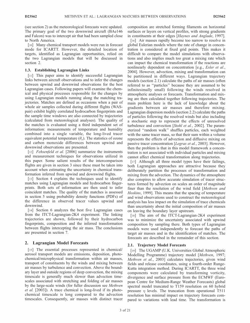
would also be likely to be polluted, emission tracers werecalculated. Gridded estimates of surface emissions wereconverted to volume sources by assuming instantaneousmixing throughout the depth of the boundary layer. Boundarylayer depth was taken from the ECMWF model output. Thesources were then integrated along trajectories wheneverthey were within the boundary layer. The NOx emissionsinventory from the Emission Database for Global Atmo-spheric Research (EDGAR [Olivier et al., 1999]) was usedto estimate the influence of anthropogenic emissions and theisoprene emissions inventory from Guenther et al. [1995]was used to indicate the influence of biogenic emissions (asa monthly mean). Clearly, both of these species have shortlifetimes (less than a day) so the emission tracers have muchhigher concentrations than could be observed along flights.Lagrangian opportunities were filtered on the basis that theanthropogenic emission tracer accumulated along backtrajectories must exceed a threshold (10 ppbv) and theaccumulated emissions along forward trajectories must staybelow the same threshold. In this way, targets were identi-fied with air masses leaving the continental boundary layerthat would also pass within range of downwind aircraft.[23] Figure 1 shows an example of an emission tracer

forecast for the U.S. east coast domain for a verificationtime 1200 UT 15 July 2004, based on an ECMWF forecaststarting from 1200 UT 13 July 2004. The air near points Aand B was also forecast to pass within range of the Azoresand Europe. The NOAA WP-3D aircraft was directed intotargets A and B and the NASA DC8 also sampled air massB on its descent into Pease.

[24] Emission tracers were also used to visualize thepolluted air mass structure over the Atlantic. Typically theair masses are stretched and folded into thin, sloping sheets(e.g., Figure 13b in section 6.2.5) seen as filaments onhorizontal surfaces. The forecasts were used to determinethe shortest route to the target and the best level to interceptit. Then the aircraft could be directed in the along-filamentdirection, sampling the air mass at several altitudes.[25] The target location was refined further by calculating

trajectories forward from the actual flight track of theupwind aircraft. The coordinates were made available forthe calculation within hours of landing. Trajectories werereleased every 10 s along the tracks. The main displacementerrors in trajectories are in the along-filament direction[Methven and Hoskins, 1999] so by flying through theforecast location of the target filament it is likely that airof similar composition will be sampled, even if the trajec-tory match has a displacement of tens of kilometers in theretrospective analysis.[26] Clearly, the forecast trajectories from flight tracks

varied as the wind forecasts were updated, but qualitativelythe set of trajectories retained similar shapes even though thefirst forecasts (for example 7 days forward from T+72 hoursinto the meteorological forecast) are based on wind forecastsextending to very long lead times (10 days). On manyoccasions the targets sampled upwind drifted out of rangeof the downwind aircraft as the forecast lead time reduced,but in many cases the targets remained within range andwere sampled (see section 6 for the best cases).

2.2. Lagrangian Dispersion Model Forecasts

[27] During ICARTT forecasts were also made usingFLEXPART, a Lagrangian particle dispersion model thatsimulates transport (by resolved winds), diffusion, dry andwet deposition. Details of the model are recorded by Stohl etal. [2005]. In its backward in time (retroplume) mode,FLEXPART has been shown to simulate measurements oflong-lived trace constituents at ground-based sites and alongaircraft tracks to the extent that potential source contribu-tions from different regions can be determined with someconfidence [Forster et al., 2001; Stohl et al., 2002, 2003].[28] During the ICARTT period FLEXPART was run

forward in time. About 100000 particles were released perday with locations weighted by an emission inventory suchthat each particle is associated with the same mass of CO onrelease. North American emissions were based on the point,onroad, nonroad and area sources from the U.S. EPANational Emissions Inventory (area sources at 4 km reso-lution) plus Mexican emissions north of 24�N and allCanadian sources south of 52�N [Frost et al., 2006]. Theinventories are estimates for the year 1999. Outside thisdomain the EDGAR emission inventory was used [Olivieret al., 1999]. Particles were carried for 20 days beforeremoval from the simulation. The positions of these par-ticles were recorded every 2 hours. The number of particlesper unit volume gives an estimate of CO concentration awayfrom the sources. FLEXPART was driven by forecasts andanalyses of winds from the Global Forecast System modelof NCEP (National Center for Environmental Prediction) at1� � 1� resolution on 26 pressure levels with a temporalresolution of 3 hours.


4 of 21

D23S62

[29] As described by Stohl et al. [2004], Lagrangianopportunities were sought by following these particlesbackward in time from the operational areas of each aircraft(Pease, Faial and Creil) and applying the following criteria:(1) The separation between the particle release point andpotential upwind link must exceed 12 hours and a distanceof 800 km. (2) The CO tracer mixing ratio must notdecrease back in time by more than 20%. (3) The RMSseparation of back trajectories released from one traceroutput cell (1� � 1� � 1000 m) must not exceed 100 kmplus 5% of travel distance. This eliminates cases with rapidback trajectory separation, indicating air being broughttogether from very different origins and therefore not agood candidate for a Lagrangian case study. The Lagrangianopportunities were ranked according to their CO tracermixing ratio weighted by the number of aircraft that couldpossibly sample it.[30] Once flights had taken place, particles were released

from boxes of size 0.7� � 0.7� � 400 m centered along theflight track and opportunities were ranked by measured CO.[31] Often the FLEXPART model with its Lagrangian

opportunity criteria highlighted different targets to theUGAMP trajectory model with its emissions tracer criteria,but on reinspection the same targets were identified by bothmodels. Each group examined the forecast products thatthey were most familiar with: FLEXPART forecasts for theNOAA WP-3D team, the UGAMP RDF forecasts for theITOP-UK team and both for the Falcon team. Agreementspotted during discussion lent weight to the decision topursue a target. FLEXPART forecasts were focussed towardplanning the upstream flights and were particularly useful inruling out cases when dilution by mixing was predicted tobe too great for the chemical contrast of the air mass toremain distinct.

[32] Comparison was also important because the twoLagrangian models used forecast winds from differentmeteorological centers (primarily for reasons of data access)which could introduce differences in target locations ofseveral hundred km on the European side of the Atlantic,especially at long lead times. The differences were used toindicate robustness in forecast Lagrangian opportunities.[33] It will be shown in section 5 that both models result

in a similar quality of coincident matches, although there aremany cases where only one of the models identifies a matchdue to the very strict, but differing, selection criteria. In thematching analysis FLEXPART was also driven by ECMWFanalyses.

3. Airborne Measurements

[34] The instruments on the four aircraft participating inthe ITCT-Lagrangian-2K4 experiment and the character-istics of their measurements are summarized by Fehsenfeldet al. [2006].[35] In order to infer changes in chemical composition

following air masses, it was crucial to compare the measure-ments by the different aircraft flying in formation as closetogether as possible. Three comparison flights were madebetween the WP-3D and DC8 on 22 July, 31 July and7 August. The DC8 and BAe146 made a rendezvous overthe mid-Atlantic on 28 July. Two comparison flights weremade between the BAe146 and Falcon: over England on7 July and over France on 3 August.[36] The ozone comparison is of particular interest since it

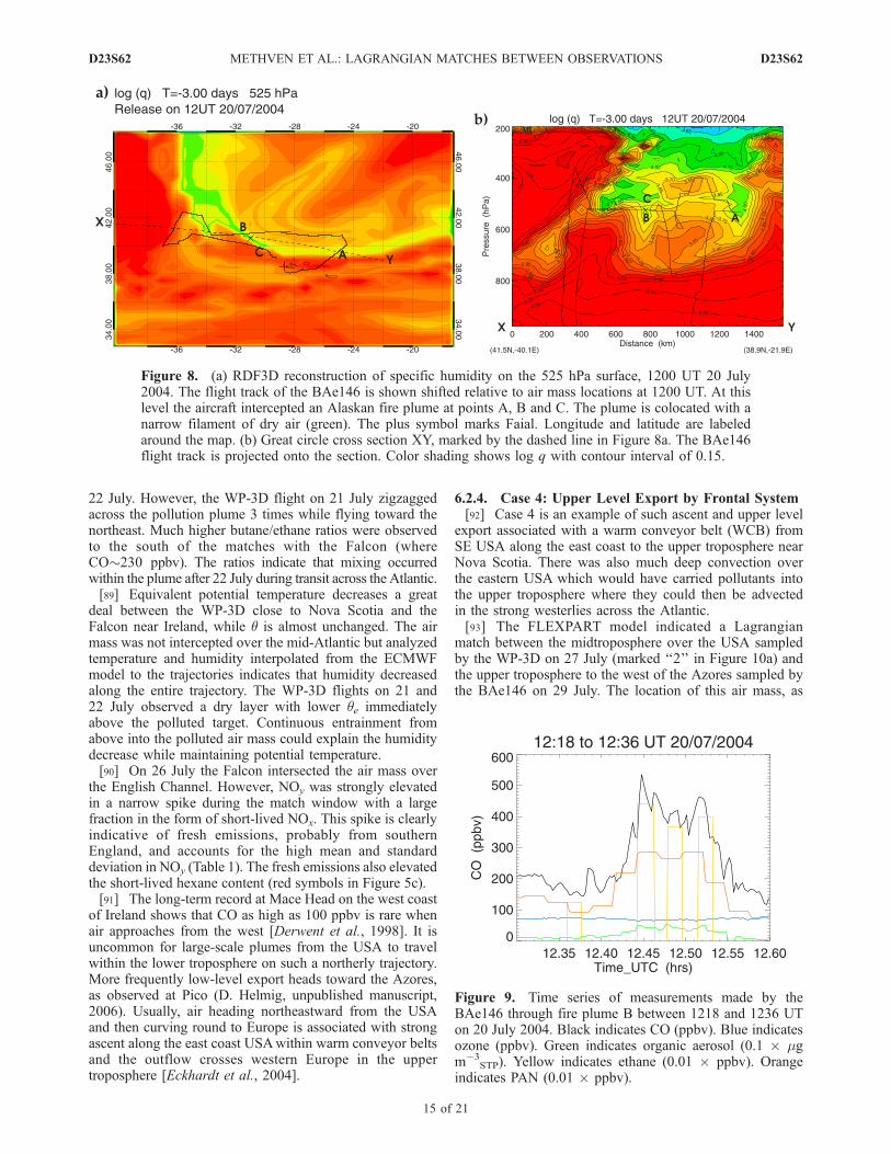
provides estimates of the limits on the determination of thenet ozone production imposed by measurement uncertainty.During each of six comparison flights the ozone measure-ments were well correlated and exhibited only small sys-

Figure 1. The 48 hour forecast depicting NOx emission tracer at 900 hPa in the U.S. domain for theverification time 1200 UT 15 July 2004. A and B mark Lagrangian targets identified from the forecast.The flight track of the NOAAWP-3D aircraft from Pease, New Hampshire (point P), is overlain. Contourinterval is 1 ppbv.


5 of 21

D23S62

tematic differences. The results indicate that the averageozone measurements agree within ±2 ppbv and the 1-sigmaprecision of the 1-s average data is better than � 1 ppbv[Fehsenfeld et al., 2006].[37] For CO, the comparison between the DC8 and

BAe146 was hindered by the lack of data from the fastresponse LARC DACOM instrument on the DC8 on28 July. However, whole air samples on the DC-8 wereanalyzed for CO to provide a comparison with the BAe146on 28 July and with the fast response CO data on the otherDC-8 flights throughout the ICARTT campaign. The resultsindicate that the average CO measurements agree within±3 ppbv for the DC-8, WP-3D and DLR Falcon, but arebiased low by 4 ppbv on the BAe146. The 1-sigmaprecision of the 1-s average data is better than �2 ppbvon all four aircraft.[38] Ambient air samples were circulated to the labora-

tories of the different groups associated with each aircraft.The hydrocarbon measurements were highly consistent[Lewis et al., 2006]. It was difficult to compare whole airsamples from comparison flights because of the differentsampling times and variability within the air masses. How-ever, it is clear that the hydrocarbon fingerprints of samplestaken within one air mass are very similar (typically thestatistic defined by equation (2), r > 0.9).[39] The frequency of data recorded by instruments varies

a great deal. Throughout this paper all data are shown with10 s resolution. Higher-frequency data have been averagedover 10 s windows centered on the time stamp. Lower-frequency data (e.g., whole air samples) are repeated atevery time point throughout the sample interval. Data fromall instruments on the DC8 and BAe146 aircraft werecollated in this way into ‘‘data merges’’ for each flight.

4. Search for Lagrangian Matches

4.1. Trajectory Model Matches

[40] Trajectories were released at 10 s intervals fromflight tracks and integrated forward and backward so thatall the associated ‘‘air masses’’ were followed over the same35 day time interval (1200 UT 1 July 2004 to 5 August 2004).The four ITCT-Lagrangian-2K4 aircraft made 40 flightsduring the period of opportunity (6 July 2004 to 1 August2004 plus the flights of the BAe146 and Falcon on 3 August),requiring 91901 trajectories from flight tracks. A timepoint on a flight was labeled as a match if its associatedtrajectory shadowed a trajectory from another flight overthe time window between the flights. If the flights wereseparated by less than 4 days, the comparison timewindow is extended to 4 days centered on the midtimebetween the flights. The criteria for ‘‘shadowing’’ wastaken to be a mean difference in latitude and equivalentpotential temperature (qe) of less than 0.5� and 2 Krespectively, averaged over the trajectory time window.For the comparison, qe was interpolated from theECMWF analyses to points spaced at 6 hour intervalsalong the trajectories. Note that often the magnitude ofchange in (analyzed) qe following a trajectory over thetime window is much greater than 2 K (e.g., associatedwith mixing or radiative cooling) but a similar evolutionmust occur for both trajectories in a matching pair suchthat their average separation is less than 2 K.

[41] In principal the match criteria based on two variablesalone could allow erroneous matches where a pair oftrajectories followed the same history of latitude and qebut at different longitudes or altitudes. However, not asingle case occurred out of the 4.1 � 109 trajectory pairs,indicating that there is negligible chance for trajectories toshadow each other this closely over a 4 day window unlessthey are within neighboring air masses.[42] A single trajectory from flight A may ‘‘match’’ with

many trajectories from flight B. Conversely, any one ofthose matching trajectories from flight B may match withmany other trajectories from flight A (‘‘converse matches’’).The many-many relationship is complex, even if only onedistinct air mass links the flights, because the two flightswill have spent different times within the air mass and mayhave intersected it on several occasions. No trajectory fromflight A matches a trajectory from flight B exactly. Thecomplexity is reduced by selecting the ‘‘best’’ matchingtrajectory from flight B for every time point along flight A.The definition of best is also problematic. One could choosethe match with the smallest latitudinal separation for exam-ple. However, this may select air masses that were sampledfor a very brief time. The chosen method was to select thetrajectory from flight B that has the most converse matcheswith flight A. In this way the ‘‘best match trajectories’’ arethe most representative of a coherent ensemble of trajecto-ries that match both flights. These trajectory-only (best)matches are marked by color bars on the time series shownin Figure 2a. Considering all ITCT-Lagrangian-2K4 flightsthere are 30887 best matching pairs.

4.2. FLEXPART Model Matches

[43] CO tracers were simulated by running the Lagrangiandispersion model FLEXPART forward in time as for theforecasts (section 2.2). The flight tracks were divided intosegments with intervals of 0.2 degrees from horizontal flightlegs (or whenever the aircraft altitude changed by more than50 m below 300 m, 150 m below 1000 m, 200 m below3000 m or 400 m above this). All particles located within30 km horizontally and 200 m vertically of a segment wereidentified and traced forward for a maximum of 10.5 days.The centroid position of these particles and their standarddeviation about the centroid was calculated. The NorthAmerican CO tracer was determined at all particle positionsand averaged over those from each flight segment.[44] Matches were defined on the basis of the same criteria

used for the identification of Lagrangian opportunities, butwith different trajectory separation criteria. The horizontaldistance between the plume centroid trajectory and down-wind measurement point plus the plume standard deviationmust be less than 18% of the distance traveled. The verticalseparation between the plume centroid trajectory and ameasurement plus the standard deviation must be less than1000 m plus 0.02% of the horizontal distance traveled.[45] In total, 395 FLEXPART ‘‘Lagrangian cases’’ were

identified and ranked according to the distance criteriaabove. By the time a plume has reached the mid-Atlanticthese two criteria are generally less strict than the trajectorymatch criteria (latitude separation < 0.5� and qe separation< 2 K). Some of these cases involved more than two aircraftflights and these were given greater weight in the ranking.


6 of 21

D23S62

In total there were 489 matches between flight time seg-ments. These are marked by red triangles in Figure 2a.[46] Although far fewer FLEXPART matches are

depicted than trajectory matches, in section 4.4 it will beshown that a similar number of coincident matches arepulled out by both models. This is because a much higherfraction of FLEXPART matches are coincident matches.Also many trajectory matches (up to 200) can be linked toone hydrocarbon match and only the best is indicated as the‘‘coincident match.’’

4.3. Hydrocarbon Fingerprinting

[47] Multicomponent hydrocarbon measurements providea means for distinguishing air masses because their relativeamounts are variable. In addition, photochemical ageing canbe inferred from compounds with a range of differentlifetimes with respect to OH reaction [e.g., Jobson et al.,1998]. If a polluted air mass mixes with a clean background,containing almost zero hydrocarbon concentrations, then theratio of any two hydrocarbons only evolves because of theirdifferent photochemical loss rates. Problems with compar-ing absolute concentrations from upwind and downwind

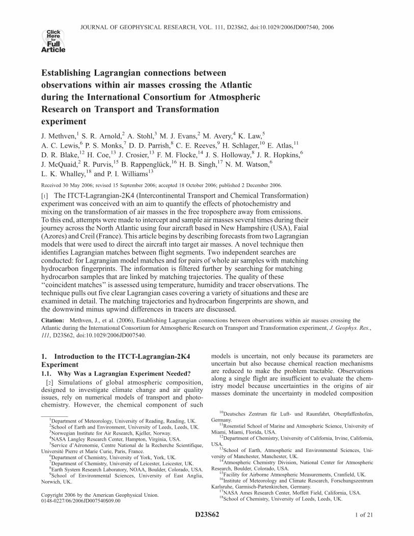
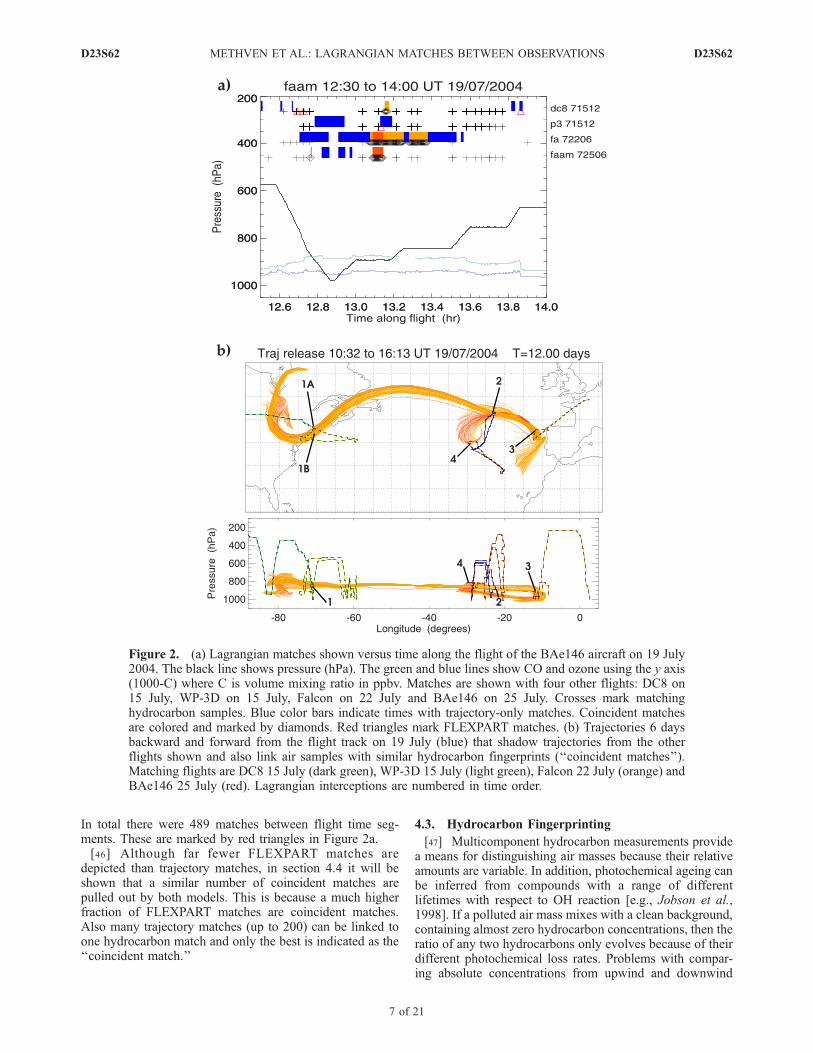
Figure 2. (a) Lagrangian matches shown versus time along the flight of the BAe146 aircraft on 19 July2004. The black line shows pressure (hPa). The green and blue lines show CO and ozone using the y axis(1000-C) where C is volume mixing ratio in ppbv. Matches are shown with four other flights: DC8 on15 July, WP-3D on 15 July, Falcon on 22 July and BAe146 on 25 July. Crosses mark matchinghydrocarbon samples. Blue color bars indicate times with trajectory-only matches. Coincident matchesare colored and marked by diamonds. Red triangles mark FLEXPART matches. (b) Trajectories 6 daysbackward and forward from the flight track on 19 July (blue) that shadow trajectories from the otherflights shown and also link air samples with similar hydrocarbon fingerprints (‘‘coincident matches’’).Matching flights are DC8 15 July (dark green), WP-3D 15 July (light green), Falcon 22 July (orange) andBAe146 25 July (red). Lagrangian interceptions are numbered in time order.


7 of 21

D23S62

samples of an air mass with variable concentrations, butdistinct composition, are to some extent circumvented byconsidering ratios.[48] Parrish [2006] examines the difficulties in using

hydrocarbon ratios to infer age of air (since leaving thesource region) that arise because air masses mix with othersthat are not clean and have different fingerprints becausethey have experienced different sources. The distribution ofsources can be estimated using the footprint of a retroplumecalculation using a Lagrangian dispersion model. It istypically found that when following a retroplume backwardin time it spreads slowly until close to the boundary layer.Here, it will be assumed that the upwind measurements aretaken above the boundary layer and that little mixing occursbefore the downwind measurements. Under these assump-tions, upwind and downwind air samples can be describedas having the same composition if their fingerprints ofhydrocarbon ratios match, after accounting for the evolutionassociated with OH loss. A. Arnold et al. (Statisticalinference of OH concentrations and air mass dilution ratesfrom successive observations of non-methane hydrocarbonsin single air masses, submitted to Journal of GeophysicalResearch, 2006, hereinafter referred to as Arnold et al.,submitted manuscript, 2006) infer the mixing rate averagedalong trajectories in addition to the OH concentration byassuming different backgrounds, estimated from theobservations.[49] Hydrocarbon fingerprints were compared between all

pairs of ‘‘whole air samples’’ (WAS pairs) collected by thefour aircraft. Matches were identified in the following way.[50] 1. The concentration ratio, hi, of 7 hydrocarbons to

ethane is found for upwind and downwind flights (to factorout dilution by mixing to a clean background). The hydro-carbons used in order of increasing reactivity with OH are:acetylene, propane, benzene, iso-butane, n-butane, pentaneand hexane (i = 1,..,7).[51] 2. The upwind ratios are adjusted to account for

photochemical loss between measurement times by takinglogs and using the rate coefficients for OH reaction, ki,assuming a constant OH concentration:

yi ¼ ln hi t1ð Þð Þ � ki � kethaneð Þ OH½ � t2 � t1ð Þ ð1Þ

where t1 and t2 are the upwind and downwind sample times,and yi is described as the ‘‘adjusted upwind ratio.’’[52] 3. For each WAS pair the scatter plot of downwind

and adjusted upwind ratios is compared with the 1:1 lineand closeness of fit measured with the statistic:

r ¼ 1�

ffiffiffiffiffiffiffiffiffiffiffiffiffiffiffiffiffiffiffiffiffiffiffiffiffiffiffiffiffiffiffiffiffiffiffi1

N�1

P12yi � xið Þ2

q

Xð2Þ

where xi = ln (hi(t2)) and X exceeds the maximum range ofx values in the data (X = 6). Note that the closest point onx = y to a measurement pair (xi, yi) is x = y = 1

2(xi + yi)

separated by the distance-squared 12(yi � xi)

2. Therefore thequantity 1 � r equals the RMS deviation from the line x = ydivided by the range in the data. N is the number ofhydrocarbons (in addition to ethane) measured in commonon both flights (cases where N < 3 were rejected).

[53] 4. The pair is labeled a ‘‘WAS match’’ if r exceedsthe 90th percentile obtained using all WAS pairs from thatpair of aircraft.[54] 5. The matching procedure was repeated for varying

OH to find the concentration that gave the highest value forr at the 50th and 90th percentiles. It was found that theidentification of Lagrangian matches is quite insensitive tovariations in OH in the range 0 to 4 � 106 molec cm�3

because the longest-lived compounds are barely affected bythe OH adjustment. A concentration of 2 � 106 molec cm�3

was used to define WAS matches. The trans-Atlanticmatches are most sensitive because of the long time elapsedbetween samples. Arnold et al. (submitted manuscript,2006) infer similar OH concentrations using a more rigor-ous method for each Lagrangian case (see section 6)allowing for mixing and taking into account measurementuncertainties and observed variability within air masses.The OH value is consistent with global estimates by Prinnet al. [1995].[55] In total there are 239608 matches meeting the

fingerprint criteria. However, most of the WAS matchesbetween samples collected by the DC8 and the WP-3D arenot linked by trajectories but simply reflect the degree ofsimilarity between air masses over the east coast USA, closeto the emissions. When DC8-DC8, P3-P3 and DC8-P3matches are excluded, the number of matches reduces to50582. WAS matches are marked by crosses on the timeseries in Figure 2a.

4.4. Coincident Matches

[56] A search was made for the subset of all matchtrajectories that link both time segments associated with aWAS pair. Every WAS measurement was associated with a6 min time segment in searching for linking trajectories.Samples typically take less than a minute to fill but thewindow was extended to allow for phase errors in thematching trajectories. These ‘‘coincident matches’’ aremarked by the diamonds and a color bar on Figure 2a.The color corresponds with the color of the matching flighttrack shown in Figure 2b.[57] All the ‘‘coincident match’’ trajectories from the

BAe146 flight track (dark blue) on 19 July are shown inFigure 2b extending 6 days backward and 6 days forward.The coincident trajectories’ colors correspond with the lastflight that they intersect.[58] Using all 40 ITCT-Lagrangian-2K4 flights, only 576

WAS matches were also linked by matching trajectories.Since the trajectories are released every 10 s from the flighttracks, there are typically many matching trajectories asso-ciated with each of these cases. These will be called‘‘coincident match trajectories’’: 8847 were found betweenall ICARTT flights, reducing to 1276 coincident matcheswhen those between the USA aircraft are excluded (DC8-DC8, P3-P3, DC8-P3).[59] A similar search was made for all FLEXPART

matches that link with both ends of a WAS match (calledFH-linked for FLEXPART-Hydrocarbon). The time seg-ments centered on the time stamp for WAS samples andFLEXPART matches were given a width of 6 min and theflights were divided into 10 s intervals (just as for thetrajectories) for the purposes of these searches. 1974 FH-linked matches were found between all ICARTT flights,


8 of 21

D23S62

reducing to 527 FH-linked matches when those between theUSA aircraft are excluded (DC8-DC8, P3-P3, DC8-P3).[60] Finally, consistency between the two models and

WAS matches is investigated by searching for coincidentmatch trajectories that link with both time segments of eachFLEXPART match (called CF-linked for coincident FLEX-PART). All the matches and corresponding time stamps arelisted at http://www.met.rdg.ac.uk/swrmethn/icartt. Onlythe best five Lagrangian cases will be discussed in section 6.

5. Evaluation of Matches Using IndependentTracer Observations

[61] The quality of the independent model and hydrocar-bon matches and their coincident matches is assessed usingfurther independent data sets: measurements of temperature,humidity, CO and ozone. A running median filter with atime window of 6 min was passed through all the time seriesof aircraft data. A running median was used (rather thanrunning mean) because it preserves the location and gradi-ent associated with boundaries between distinct air masses,while removing rapid fluctuations that cannot be associatedwith particular trajectory behavior. It has little impact on thetime series far from emissions, but smooths out rapidfluctuations over the USA close to sources, especially inthe boundary layer. The filtered aircraft data is interpolatedto the release points used for the trajectories (at 10 sintervals). Differences between upwind and downwindpotential temperature (q), equivalent potential temperature(qe), CO and ozone are calculated for every match. PDFs ofthese differences are plotted for the various methods:trajectory matches, WAS matches, coincident matches andFH-linked matches.

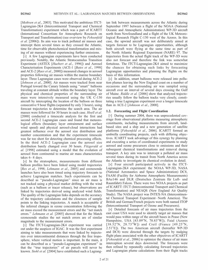
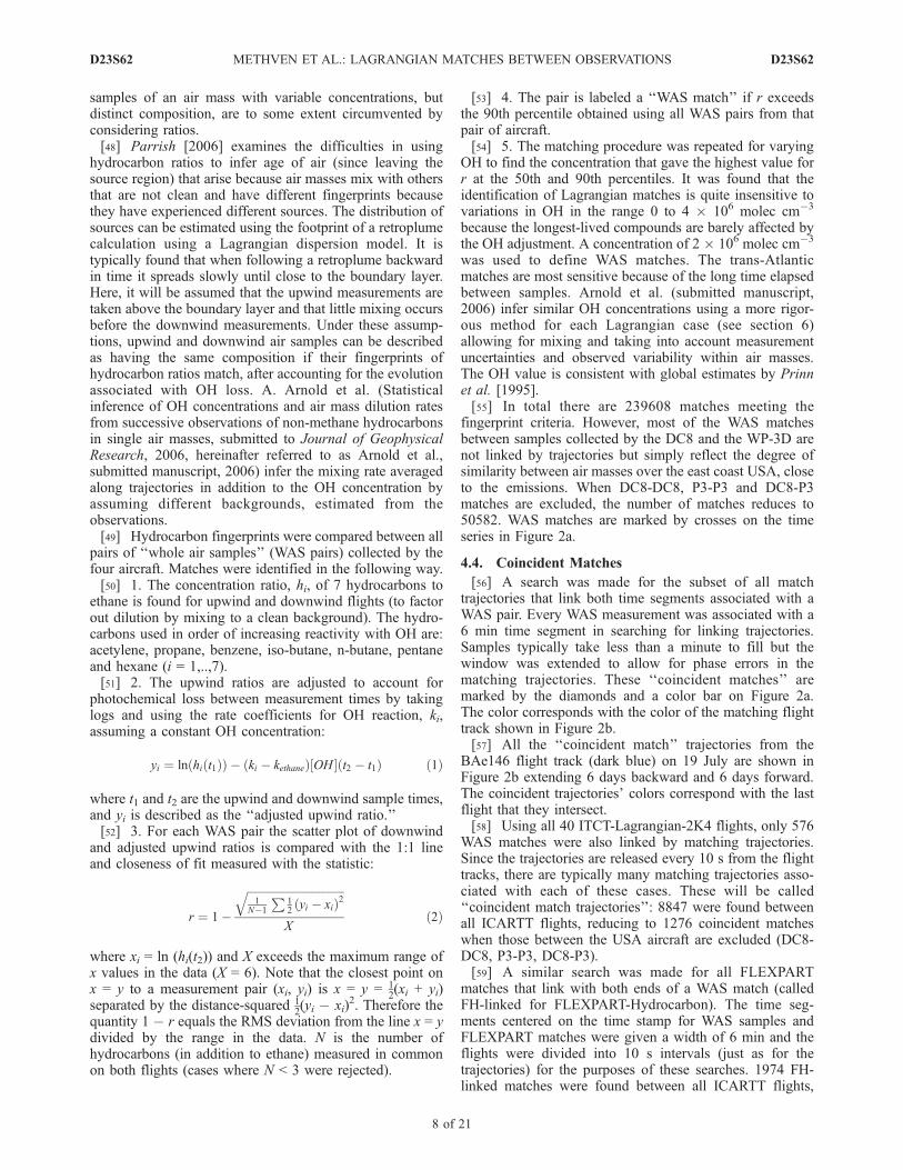
[62] The potential temperature difference between down-wind and upwind samples is divided by their time separa-tion to give the average rate of change following air masses.The resulting PDF (Figure 3a) is strongly peaked on slowcooling (0 to �2 K day�1) for coincident trajectory-hydrocarbon matches and a similar PDF is obtained usingFLEXPART-hydrocarbon (FH-linked) matches. This valueis consistent with constant radiative cooling under clearskies. The trajectory-only matches are also strongly peakednear zero, indicating that most of the trajectories that matchare almost isentropic. In contrast, the PDF for WAS matchesis much flatter indicating that many samples with similarhydrocarbon fingerprints are not within the same air mass(i.e., not linked by trajectories).[63] Note that the black curve was obtained by selecting

n time points at random from the time series of two flightsand using observed q from these pairs of points tocalculate (q2 � q1)/(t2 � t1). Each pair of flights wasweighted by setting n equal to the number of trajectorymatches between them. The ‘‘random’’ histogram illus-trates the similarity of the air masses sampled on flightsthat are linked, irrespective of Lagrangian connections.Therefore its values cannot be interpreted as heating ratesfollowing air masses. The identification of Lagrangianmatches is only successful if the PDF for matches is morestrongly peaked than the PDF for randomly selected timepoints. Clearly, WAS matches alone are not significantlydifferent from random selection.[64] Note that the coincident and FH-linked PDFs have a

secondary peak at a heating rate of about 5 K day�1. Thiscan be attributed to the time-averaged rate of latent heatrelease in ascending air masses. A better thermodynamictracer of air masses is equivalent potential temperature, qe,that is conserved for the pseudoadiabatic process of asaturated air mass experiencing condensation. The PDFsfor rate of change of qe (Figure 3b) are even more stronglypeaked on weak cooling for coincident and FH-linkedmatches. Trajectory-only matches are clearly not as goodas coincident matches. qe reveals that although trajectorymatches may occur in the same isentropic layer (range ofq values) they can have the wrong specific humidity for aLagrangian match. The additional requirement for ahydrocarbon match pulls out the matches with similarhumidity. Conversely, the PDF for WAS matches is morepeaked for qe than for q. This shows that the qe signatureand hydrocarbon fingerprint are correlated, both beingindicative of air mass origin, even if two samples are notlinked by trajectories.[65] Upwind and downwind matching observations are

used to estimate ‘‘growth rates’’ for Figure 4 using:

sc ¼1

t2 � t1lnC2 � lnC1ð Þ ð3Þ

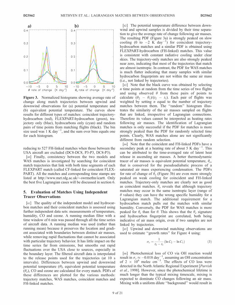
[66] Photochemical loss of CO via OH reaction wouldresult in sc � �0.018 day�1, assuming an OH concentrationof 2 � 106 molec cm�3. The effects of CO loss weredetected in the North Atlantic Regional Experiment [Parrishet al., 1998]. However, since the photochemical lifetime ismuch longer than the typical mixing timescale, mixing isexpected to dominate CO changes following an air mass.Mixing with a uniform dilute ‘‘background’’ would result in

Figure 3. Normalized histograms showing average rate ofchange along match trajectories between upwind anddownwind observations for (a) potential temperature and(b) equivalent potential temperature. The curves showresults for different types of matches: coincident trajectory-hydrocarbon (red), FLEXPART-hydrocarbon (green), tra-jectory only (blue), hydrocarbons only (cyan) and randompairs of time points from matching flights (black). The binsize used was 1 K day�1, and the sum over bins equals onefor each histogram.


9 of 21

D23S62

exponential decay of concentration with timescale �1/sc.However, typically pollution plumes do not have muchhigher CO concentrations than their surroundings, sinceCO is rather long-lived, and dilution of CO within the centerof the plume will be slow even if turbulent mixing is active.In this case, �1/sc cannot be interpreted as a turbulentmixing timescale. The narrow PDF peak for ‘‘CO growthrate’’ occurs between 0 and �0.1 day�1, indicative of a slowdilution timescale exceeding 10 days. Weak CO increase isinferred from some match pairs. This is most likely to resultfrom a slight mismatch in a plume with high variability. Forexample the downwind flight may have crossed the maxi-mum plume concentration while the upwind aircraft mayhave sampled only the flanks or flown just above or belowthe air mass sampled downstream.[67] The ‘‘ozone growth rate’’ PDF for coincident

matches peaks just above zero, consistent with slow photo-chemistry and mixing. The positive peak is perhaps attrib-utable to net photochemical ozone production in thepolluted Lagrangian matches. Stronger decrease and in-crease is seen for a few matches. Photochemical modelingeffort to explain the observations will be focussed on thebest Lagrangian cases described in the next section.

6. Best ITCT-Lagrangian-2K4 Cases

6.1. Observed Hydrocarbon Fingerprints

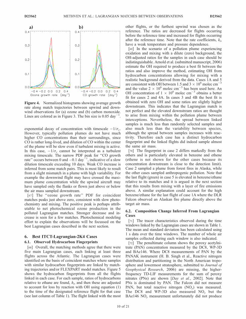
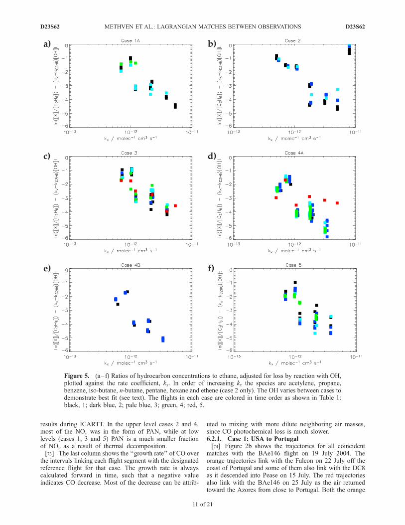
[68] Overall, the matching methods agree that there werefive main Lagrangian cases, each linking at least threeflights across the Atlantic. The Lagrangian cases wereidentified on the basis of coincident matches where sampleswith similar hydrocarbon fingerprints are linked by match-ing trajectories and/or FLEXPART model matches. Figure 5shows the hydrocarbon fingerprints from all the flightslinked in each case. For each sample, ratios of hydrocarbonsrelative to ethane are found, hi, and then these are adjustedto account for loss by reaction with OH using equation (1)to the time of the designated reference flight for that case(see last column of Table 1). The flight linked with the most

other flights, or the furthest upwind was chosen as thereference. The ratios are decreased for flights occurringbefore the reference time and increased for flights occurringafter the reference time. Note that the rate coefficients, ki,have a weak temperature and pressure dependence.[69] In the scenario of a pollution plume experiencing

oxidation and mixing with a dilute (zero) background, theOH-adjusted ratios for the samples in each case should beindistinguishable. Arnold et al. (submitted manuscript, 2006)estimate the OH required to produce a best fit between theratios and also improve the method, estimating OH fromhydrocarbon concentrations allowing for mixing with arealistic background derived from the data. Cases 1A and 5are consistent with OH between 1.5 and 3� 106 molec cm�3

and the value 2 � 106 molec cm�3 has been used here. AnOH concentration of 1 � 106 molec cm�3 obtains a betterfit for cases 2 and 4A. In cases 3 and 4B the best fit isobtained with zero OH and some ratios are slightly higherdownstream. This indicates that the Lagrangian match isnot perfect and the elevated downstream ratios are thoughtto arise from mixing within the pollution plume betweeninterceptions. Nevertheless, the spread between linkedsamples is much less than randomly selected samples andalso much less than the variability between species,although the spread between samples increases with reac-tivity. Therefore each case has a distinct hydrocarbonfingerprint and the linked flights did indeed sample almostthe same air mass.[70] The fingerprint in case 2 differs markedly from the

others and is particularly elevated in benzene and ethene(ethene is not shown for the other cases because itsconcentration downstream is close to the detection limit).Case 2 sampled a plume from forest fires in Alaska, whilethe other cases sampled anthropogenic pollution. Note thatthe last flight (green) in case 5 is elevated in benzene/ethanerelative to its matches and it is argued in the next sectionthat this results from mixing with a layer of fire emissionsabove. A similar explanation could account for the highbenzene/ethane for the last flight of case 1Awhere the DLRFalcon observed an Alaskan fire plume directly above thetarget air mass.

6.2. Composition Change Inferred From LagrangianCases

[71] The tracer characteristics observed during the timewindows linked by the Lagrangian cases are shown in Table 1.The mean and standard deviation has been calculated using1 s data over the time windows. The number of whole airsamples collected during each window is also indicated.[72] The penultimate column shows the peroxy acetylni-

trate (PAN) concentration measured by the DC8, WP-3Dand BAe146. Where DC8 measurements of PAN by thePANAK instrument (H. B. Singh et al., Reactive nitrogendistribution and partitioning in the North American tropo-sphere and lowermost stratosphere, submitted to Journal ofGeophysical Research, 2006) are missing, the higher-frequency TD-LIF measurements for the sum of peroxynitrates (PNs) are shown [Day et al., 2002]. Note thatPNs is dominated by PAN. The Falcon did not measurePAN, but total reactive nitrogen (NOy) was measured.The DC8 and WP-3D also measured NOy but theBAe146 NOy measurement unfortunately did not produce

Figure 4. Normalized histograms showing average growthrate along match trajectories between upwind and down-wind observations for (a) ozone and (b) carbon monoxide.Lines are colored as in Figure 3. The bin size is 0.05 day�1.


10 of 21

D23S62

results during ICARTT. In the upper level cases 2 and 4,most of the NOy was in the form of PAN, while at lowlevels (cases 1, 3 and 5) PAN is a much smaller fractionof NOy as a result of thermal decomposition.[73] The last column shows the ‘‘growth rate’’ of CO over

the intervals linking each flight segment with the designatedreference flight for that case. The growth rate is alwayscalculated forward in time, such that a negative valueindicates CO decrease. Most of the decrease can be attrib-

uted to mixing with more dilute neighboring air masses,since CO photochemical loss is much slower.6.2.1. Case 1: USA to Portugal[74] Figure 2b shows the trajectories for all coincident

matches with the BAe146 flight on 19 July 2004. Theorange trajectories link with the Falcon on 22 July off thecoast of Portugal and some of them also link with the DC8as it descended into Pease on 15 July. The red trajectoriesalso link with the BAe146 on 25 July as the air returnedtoward the Azores from close to Portugal. Both the orange

Figure 5. (a–f) Ratios of hydrocarbon concentrations to ethane, adjusted for loss by reaction with OH,plotted against the rate coefficient, kx. In order of increasing kx the species are acetylene, propane,benzene, iso-butane, n-butane, pentane, hexane and ethene (case 2 only). The OH varies between cases todemonstrate best fit (see text). The flights in each case are colored in time order as shown in Table 1:black, 1; dark blue, 2; pale blue, 3; green, 4; red, 5.


11 of 21

D23S62

and red trajectories shadow trajectories from the WP-3Dflight on 15 July (close to point B on Figure 1) but becauseof a system malfunction no WAS measurements were madeon this half of the flight and therefore hydrocarbon finger-prints cannot be compared. However, the match with theWP-3D is also indicated by the FLEXPART model (redtriangle in Figure 2a).[75] Further examination reveals two distinct cases: co-

incident matches along the DC8 track occur with theBAe146 19 July at higher altitude (855 hPa) than withBAe146 25 July (902 hPa). Similarly, matches occur alongthe Falcon track with the BAe146 19 July at 913 hPa(orange trajectories) but with the BAe146 25 July on alower-level run (at 965 hPa) within the marine boundarylayer (red trajectories). Therefore this case has been splitinto two, with case 1B occurring at slightly lower altitudethan case 1A. The split is confirmed by the distincthydrocarbon fingerprints for the two cases. Case 1B is morepolluted and has a higher butane/ethane ratio.

[76] In case 1A, the DC8 and WP-3D match windowswere separated by less than an hour and 0.35� latitude ontheir descent into Pease from the west. The WP-3D was atslightly lower altitude (887 hPa compared with DC8 win-dow average of 855 hPa) where CO and ozone were higher.PAN was not measured by the DC8 on this descent, butalmost 1 ppbv was observed by the WP-3D.[77] Another segment along the WP-3D track which has

trajectory and FLEXPART matches with the Falcon andBAe146 is further south by about 100 km (near Cape Cod).It has been attributed to case 1B, although the WP-3Dcrossed the maximum in the plume downwind of the NewYork conurbation (level at 928 hPa) and clearly observedhigher CO and ozone than the DC8 closer to Pease.[78] Potential temperature varies little following the air

mass 1A, but qe decreases, consistent with a decrease inspecific humidity while maintaining constant temperaturebetween Pease and the BAe146 on 19 July (as occurs incase 3). The CO mixing ratio decreases with time but at asurprisingly slow rate indicating a 1/sc timescale in the

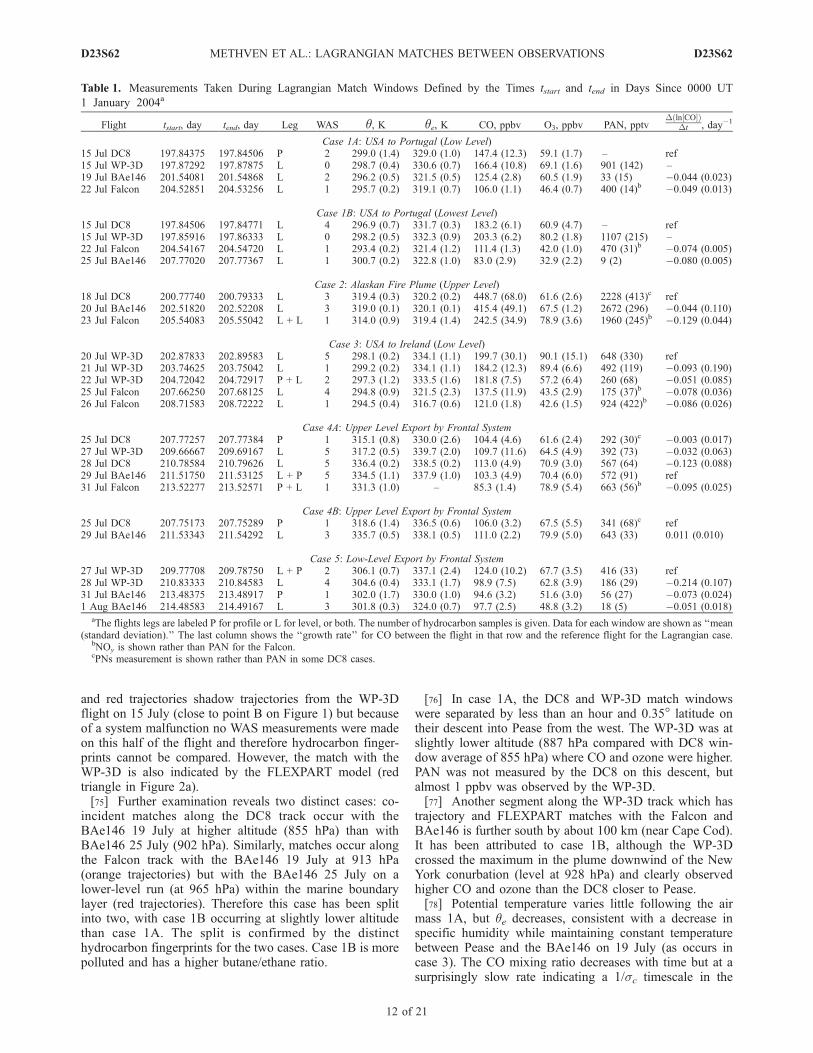
Table 1. Measurements Taken During Lagrangian Match Windows Defined by the Times tstart and tend in Days Since 0000 UT

1 January 2004a

Flight tstart, day tend, day Leg WAS q, K qe, K CO, ppbv O3, ppbv PAN, pptvD ln CO½ �ð Þ

Dt , day�1

Case 1A: USA to Portugal (Low Level)15 Jul DC8 197.84375 197.84506 P 2 299.0 (1.4) 329.0 (1.0) 147.4 (12.3) 59.1 (1.7) – ref15 Jul WP-3D 197.87292 197.87875 L 0 298.7 (0.4) 330.6 (0.7) 166.4 (10.8) 69.1 (1.6) 901 (142) –19 Jul BAe146 201.54081 201.54868 L 2 296.2 (0.5) 321.5 (0.5) 125.4 (2.8) 60.5 (1.9) 33 (15) �0.044 (0.023)22 Jul Falcon 204.52851 204.53256 L 1 295.7 (0.2) 319.1 (0.7) 106.0 (1.1) 46.4 (0.7) 400 (14)b �0.049 (0.013)

Case 1B: USA to Portugal (Lowest Level)15 Jul DC8 197.84506 197.84771 L 4 296.9 (0.7) 331.7 (0.3) 183.2 (6.1) 60.9 (4.7) – ref15 Jul WP-3D 197.85916 197.86333 L 0 298.2 (0.5) 332.3 (0.9) 203.3 (6.2) 80.2 (1.8) 1107 (215) –22 Jul Falcon 204.54167 204.54720 L 1 293.4 (0.2) 321.4 (1.2) 111.4 (1.3) 42.0 (1.0) 470 (31)b �0.074 (0.005)25 Jul BAe146 207.77020 207.77367 L 1 300.7 (0.2) 322.8 (1.0) 83.0 (2.9) 32.9 (2.2) 9 (2) �0.080 (0.005)

Case 2: Alaskan Fire Plume (Upper Level)18 Jul DC8 200.77740 200.79333 L 3 319.4 (0.3) 320.2 (0.2) 448.7 (68.0) 61.6 (2.6) 2228 (413)c ref20 Jul BAe146 202.51820 202.52208 L 3 319.0 (0.1) 320.1 (0.1) 415.4 (49.1) 67.5 (1.2) 2672 (296) �0.044 (0.110)23 Jul Falcon 205.54083 205.55042 L + L 1 314.0 (0.9) 319.4 (1.4) 242.5 (34.9) 78.9 (3.6) 1960 (245)b �0.129 (0.044)

Case 3: USA to Ireland (Low Level)20 Jul WP-3D 202.87833 202.89583 L 5 298.1 (0.2) 334.1 (1.1) 199.7 (30.1) 90.1 (15.1) 648 (330) ref21 Jul WP-3D 203.74625 203.75042 L 1 299.2 (0.2) 334.1 (1.1) 184.2 (12.3) 89.4 (6.6) 492 (119) �0.093 (0.190)22 Jul WP-3D 204.72042 204.72917 P + L 2 297.3 (1.2) 333.5 (1.6) 181.8 (7.5) 57.2 (6.4) 260 (68) �0.051 (0.085)25 Jul Falcon 207.66250 207.68125 L 4 294.8 (0.9) 321.5 (2.3) 137.5 (11.9) 43.5 (2.9) 175 (37)b �0.078 (0.036)26 Jul Falcon 208.71583 208.72222 L 1 294.5 (0.4) 316.7 (0.6) 121.0 (1.8) 42.6 (1.5) 924 (422)b �0.086 (0.026)

Case 4A: Upper Level Export by Frontal System25 Jul DC8 207.77257 207.77384 P 1 315.1 (0.8) 330.0 (2.6) 104.4 (4.6) 61.6 (2.4) 292 (30)c �0.003 (0.017)27 Jul WP-3D 209.66667 209.69167 L 5 317.2 (0.5) 339.7 (2.0) 109.7 (11.6) 64.5 (4.9) 392 (73) �0.032 (0.063)28 Jul DC8 210.78584 210.79626 L 5 336.4 (0.2) 338.5 (0.2) 113.0 (4.9) 70.9 (3.0) 567 (64) �0.123 (0.088)29 Jul BAe146 211.51750 211.53125 L + P 5 334.5 (1.1) 337.9 (1.0) 103.3 (4.9) 70.4 (6.0) 572 (91) ref31 Jul Falcon 213.52277 213.52571 P + L 1 331.3 (1.0) – 85.3 (1.4) 78.9 (5.4) 663 (56)b �0.095 (0.025)

Case 4B: Upper Level Export by Frontal System25 Jul DC8 207.75173 207.75289 P 1 318.6 (1.4) 336.5 (0.6) 106.0 (3.2) 67.5 (5.5) 341 (68)c ref29 Jul BAe146 211.53343 211.54292 L 3 335.7 (0.5) 338.1 (0.5) 111.0 (2.2) 79.9 (5.0) 643 (33) 0.011 (0.010)

Case 5: Low-Level Export by Frontal System27 Jul WP-3D 209.77708 209.78750 L + P 2 306.1 (0.7) 337.1 (2.4) 124.0 (10.2) 67.7 (3.5) 416 (33) ref28 Jul WP-3D 210.83333 210.84583 L 4 304.6 (0.4) 333.1 (1.7) 98.9 (7.5) 62.8 (3.9) 186 (29) �0.214 (0.107)31 Jul BAe146 213.48375 213.48917 P 1 302.0 (1.7) 330.0 (1.0) 94.6 (3.2) 51.6 (3.0) 56 (27) �0.073 (0.024)1 Aug BAe146 214.48583 214.49167 L 3 301.8 (0.3) 324.0 (0.7) 97.7 (2.5) 48.8 (3.2) 18 (5) �0.051 (0.018)

aThe flights legs are labeled P for profile or L for level, or both. The number of hydrocarbon samples is given. Data for each window are shown as ‘‘mean(standard deviation).’’ The last column shows the ‘‘growth rate’’ for CO between the flight in that row and the reference flight for the Lagrangian case.

bNOy is shown rather than PAN for the Falcon.cPNs measurement is shown rather than PAN in some DC8 cases.


12 of 21

D23S62

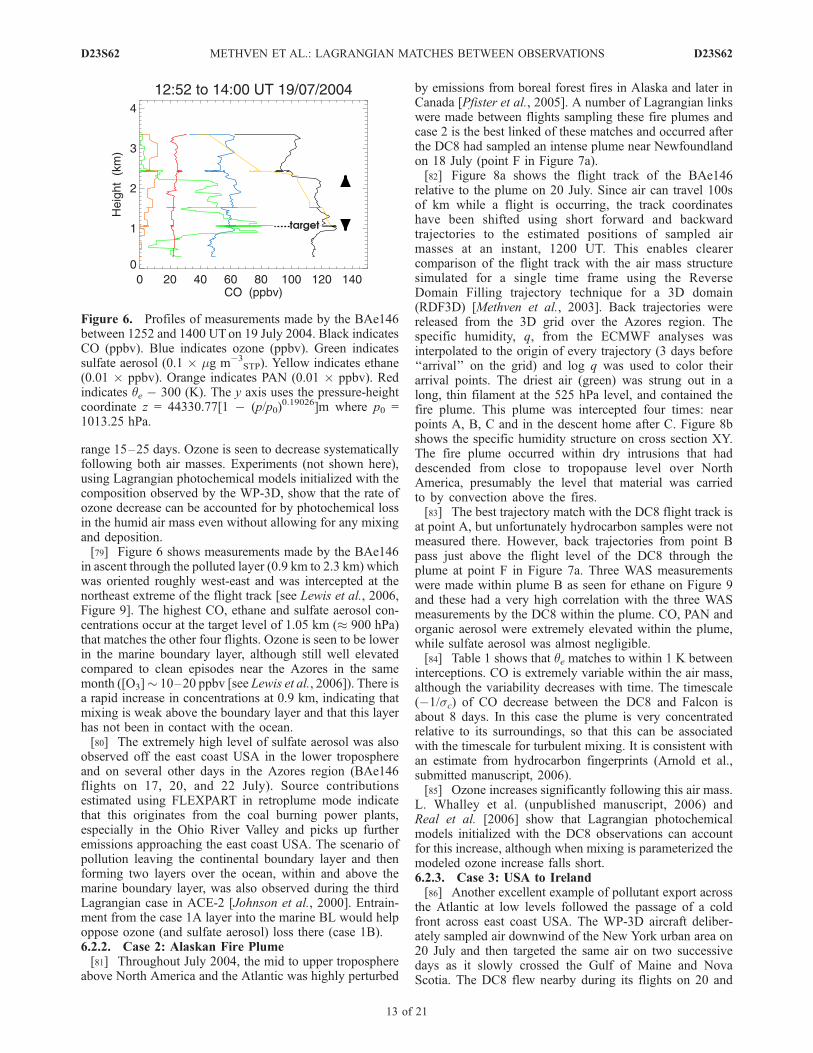
range 15–25 days. Ozone is seen to decrease systematicallyfollowing both air masses. Experiments (not shown here),using Lagrangian photochemical models initialized with thecomposition observed by the WP-3D, show that the rate ofozone decrease can be accounted for by photochemical lossin the humid air mass even without allowing for any mixingand deposition.[79] Figure 6 shows measurements made by the BAe146

in ascent through the polluted layer (0.9 km to 2.3 km) whichwas oriented roughly west-east and was intercepted at thenortheast extreme of the flight track [see Lewis et al., 2006,Figure 9]. The highest CO, ethane and sulfate aerosol con-centrations occur at the target level of 1.05 km (� 900 hPa)that matches the other four flights. Ozone is seen to be lowerin the marine boundary layer, although still well elevatedcompared to clean episodes near the Azores in the samemonth ([O3] 10–20 ppbv [see Lewis et al., 2006]). There isa rapid increase in concentrations at 0.9 km, indicating thatmixing is weak above the boundary layer and that this layerhas not been in contact with the ocean.[80] The extremely high level of sulfate aerosol was also

observed off the east coast USA in the lower troposphereand on several other days in the Azores region (BAe146flights on 17, 20, and 22 July). Source contributionsestimated using FLEXPART in retroplume mode indicatethat this originates from the coal burning power plants,especially in the Ohio River Valley and picks up furtheremissions approaching the east coast USA. The scenario ofpollution leaving the continental boundary layer and thenforming two layers over the ocean, within and above themarine boundary layer, was also observed during the thirdLagrangian case in ACE-2 [Johnson et al., 2000]. Entrain-ment from the case 1A layer into the marine BL would helpoppose ozone (and sulfate aerosol) loss there (case 1B).6.2.2. Case 2: Alaskan Fire Plume[81] Throughout July 2004, the mid to upper troposphere

above North America and the Atlantic was highly perturbed

by emissions from boreal forest fires in Alaska and later inCanada [Pfister et al., 2005]. A number of Lagrangian linkswere made between flights sampling these fire plumes andcase 2 is the best linked of these matches and occurred afterthe DC8 had sampled an intense plume near Newfoundlandon 18 July (point F in Figure 7a).[82] Figure 8a shows the flight track of the BAe146

relative to the plume on 20 July. Since air can travel 100sof km while a flight is occurring, the track coordinateshave been shifted using short forward and backwardtrajectories to the estimated positions of sampled airmasses at an instant, 1200 UT. This enables clearercomparison of the flight track with the air mass structuresimulated for a single time frame using the ReverseDomain Filling trajectory technique for a 3D domain(RDF3D) [Methven et al., 2003]. Back trajectories werereleased from the 3D grid over the Azores region. Thespecific humidity, q, from the ECMWF analyses wasinterpolated to the origin of every trajectory (3 days before‘‘arrival’’ on the grid) and log q was used to color theirarrival points. The driest air (green) was strung out in along, thin filament at the 525 hPa level, and contained thefire plume. This plume was intercepted four times: nearpoints A, B, C and in the descent home after C. Figure 8bshows the specific humidity structure on cross section XY.The fire plume occurred within dry intrusions that haddescended from close to tropopause level over NorthAmerica, presumably the level that material was carriedto by convection above the fires.[83] The best trajectory match with the DC8 flight track is

at point A, but unfortunately hydrocarbon samples were notmeasured there. However, back trajectories from point Bpass just above the flight level of the DC8 through theplume at point F in Figure 7a. Three WAS measurementswere made within plume B as seen for ethane on Figure 9and these had a very high correlation with the three WASmeasurements by the DC8 within the plume. CO, PAN andorganic aerosol were extremely elevated within the plume,while sulfate aerosol was almost negligible.[84] Table 1 shows that qe matches to within 1 K between

interceptions. CO is extremely variable within the air mass,although the variability decreases with time. The timescale(�1/sc) of CO decrease between the DC8 and Falcon isabout 8 days. In this case the plume is very concentratedrelative to its surroundings, so that this can be associatedwith the timescale for turbulent mixing. It is consistent withan estimate from hydrocarbon fingerprints (Arnold et al.,submitted manuscript, 2006).[85] Ozone increases significantly following this air mass.

L. Whalley et al. (unpublished manuscript, 2006) andReal et al. [2006] show that Lagrangian photochemicalmodels initialized with the DC8 observations can accountfor this increase, although when mixing is parameterized themodeled ozone increase falls short.6.2.3. Case 3: USA to Ireland[86] Another excellent example of pollutant export across

the Atlantic at low levels followed the passage of a coldfront across east coast USA. The WP-3D aircraft deliber-ately sampled air downwind of the New York urban area on20 July and then targeted the same air on two successivedays as it slowly crossed the Gulf of Maine and NovaScotia. The DC8 flew nearby during its flights on 20 and

Figure 6. Profiles of measurements made by the BAe146between 1252 and 1400 UTon 19 July 2004. Black indicatesCO (ppbv). Blue indicates ozone (ppbv). Green indicatessulfate aerosol (0.1 � mg m�3

STP). Yellow indicates ethane(0.01 � ppbv). Orange indicates PAN (0.01 � ppbv). Redindicates qe � 300 (K). The y axis uses the pressure-heightcoordinate z = 44330.77[1 � (p/p0)

0.19026]m where p0 =1013.25 hPa.


13 of 21

D23S62

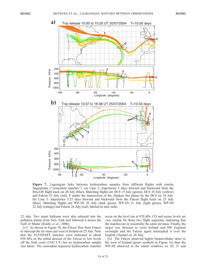
22 July. Two smart balloons were also released into thepollution plume from New York and followed it across theGulf of Maine [Riddle et al., 2006].[87] As shown in Figure 7b, the Falcon flew from France

to intercept the air mass just west of Ireland on 25 July. Notethat the FLEXPART matches were indicated at about850 hPa on the initial descent of the Falcon to low levelsoff the Irish coast (1542 UT) but no hydrocarbon samplewas taken. The coincident trajectory-hydrocarbon matches

occur on the level run at 870 hPa. CO and ozone levels arevery similar for these two flight segments, indicating thatthe matches are in essentially the same air mass. Finally, thetarget was forecast to cross Ireland and SW Englandovernight and the Falcon again intercepted it over theEnglish Channel on 26 July.[88] The Falcon observed higher butane/ethane ratios to

the west of Ireland (green symbols in Figure 5c) than theWP-3D observed in the match windows on 20, 21 and

Figure 7. Lagrangian links between hydrocarbon samples from different flights with similarfingerprints (‘‘coincident matches’’). (a) Case 2: trajectories 5 days forward and backward from theBAe146 flight track on 20 July (blue). Matching flights are DC8 15 July (green), DC8 18 July (yellow)and Falcon 23 July (red). F marks the intersection of the Alaskan fire plume by the DC8 on 18 July.(b) Case 3: trajectories 5.25 days forward and backward from the Falcon flight track on 25 July(blue). Matching flights are WP-3D 20 July (dark green), WP-3D 21 July (light green), WP-3D22 July (orange) and Falcon 26 July (red), labeled in time order.


14 of 21

D23S62

22 July. However, the WP-3D flight on 21 July zigzaggedacross the pollution plume 3 times while flying toward thenortheast. Much higher butane/ethane ratios were observedto the south of the matches with the Falcon (whereCO230 ppbv). The ratios indicate that mixing occurredwithin the plume after 22 July during transit across the Atlantic.[89] Equivalent potential temperature decreases a great

deal between the WP-3D close to Nova Scotia and theFalcon near Ireland, while q is almost unchanged. The airmass was not intercepted over the mid-Atlantic but analyzedtemperature and humidity interpolated from the ECMWFmodel to the trajectories indicates that humidity decreasedalong the entire trajectory. The WP-3D flights on 21 and22 July observed a dry layer with lower qe immediatelyabove the polluted target. Continuous entrainment fromabove into the polluted air mass could explain the humiditydecrease while maintaining potential temperature.[90] On 26 July the Falcon intersected the air mass over

the English Channel. However, NOy was strongly elevatedin a narrow spike during the match window with a largefraction in the form of short-lived NOx. This spike is clearlyindicative of fresh emissions, probably from southernEngland, and accounts for the high mean and standarddeviation in NOy (Table 1). The fresh emissions also elevatedthe short-lived hexane content (red symbols in Figure 5c).[91] The long-term record at Mace Head on the west coast

of Ireland shows that CO as high as 100 ppbv is rare whenair approaches from the west [Derwent et al., 1998]. It isuncommon for large-scale plumes from the USA to travelwithin the lower troposphere on such a northerly trajectory.More frequently low-level export heads toward the Azores,as observed at Pico (D. Helmig, unpublished manuscript,2006). Usually, air heading northeastward from the USAand then curving round to Europe is associated with strongascent along the east coast USAwithin warm conveyor beltsand the outflow crosses western Europe in the uppertroposphere [Eckhardt et al., 2004].

6.2.4. Case 4: Upper Level Export by Frontal System[92] Case 4 is an example of such ascent and upper level

export associated with a warm conveyor belt (WCB) fromSE USA along the east coast to the upper troposphere nearNova Scotia. There was also much deep convection overthe eastern USA which would have carried pollutants intothe upper troposphere where they could then be advectedin the strong westerlies across the Atlantic.[93] The FLEXPART model indicated a Lagrangian

match between the midtroposphere over the USA sampledby the WP-3D on 27 July (marked ‘‘2’’ in Figure 10a) andthe upper troposphere to the west of the Azores sampled bythe BAe146 on 29 July. The location of this air mass, as

Figure 8. (a) RDF3D reconstruction of specific humidity on the 525 hPa surface, 1200 UT 20 July2004. The flight track of the BAe146 is shown shifted relative to air mass locations at 1200 UT. At thislevel the aircraft intercepted an Alaskan fire plume at points A, B and C. The plume is colocated with anarrow filament of dry air (green). The plus symbol marks Faial. Longitude and latitude are labeledaround the map. (b) Great circle cross section XY, marked by the dashed line in Figure 8a. The BAe146flight track is projected onto the section. Color shading shows log q with contour interval of 0.15.

Figure 9. Time series of measurements made by theBAe146 through fire plume B between 1218 and 1236 UTon 20 July 2004. Black indicates CO (ppbv). Blue indicatesozone (ppbv). Green indicates organic aerosol (0.1 � mgm�3

STP). Yellow indicates ethane (0.01 � ppbv). Orangeindicates PAN (0.01 � ppbv).


15 of 21

D23S62

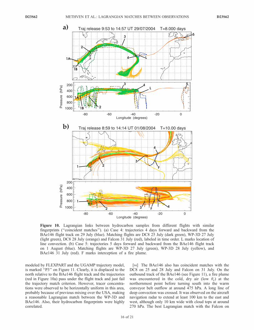
modeled by FLEXPART and the UGAMP trajectory model,is marked ‘‘P3’’ on Figure 11. Clearly, it is displaced to thenorth relative to the BAe146 flight track and the trajectories(red in Figure 10a) pass under the flight track and just failthe trajectory match criterion. However, tracer concentra-tions were observed to be horizontally uniform in this area,probably because of previous mixing over the USA, makinga reasonable Lagrangian match between the WP-3D andBAe146. Also, their hydrocarbon fingerprints were highlycorrelated.

[94] The BAe146 also has coincident matches with theDC8 on 25 and 28 July and Falcon on 31 July. On theoutbound track of the BAe146 (see Figure 11), a fire plumewas encountered in the cold, dry air (low qe) at thenorthernmost point before turning south into the warmconveyor belt outflow at around 475 hPa. A long line ofdeep convection was crossed. It was observed on the aircraftnavigation radar to extend at least 100 km to the east andwest, although only 10 km wide with cloud tops at around270 hPa. The best Lagrangian match with the Falcon on

Figure 10. Lagrangian links between hydrocarbon samples from different flights with similarfingerprints (‘‘coincident matches’’). (a) Case 4: trajectories 4 days forward and backward from theBAe146 flight track on 29 July (blue). Matching flights are DC8 25 July (dark green), WP-3D 27 July(light green), DC8 28 July (orange) and Falcon 31 July (red), labeled in time order. L marks location ofline convection. (b) Case 5: trajectories 5 days forward and backward from the BAe146 flight trackon 1 August (blue). Matching flights are WP-3D 27 July (green), WP-3D 28 July (yellow), andBAe146 31 July (red). F marks interception of a fire plume.


16 of 21

D23S62

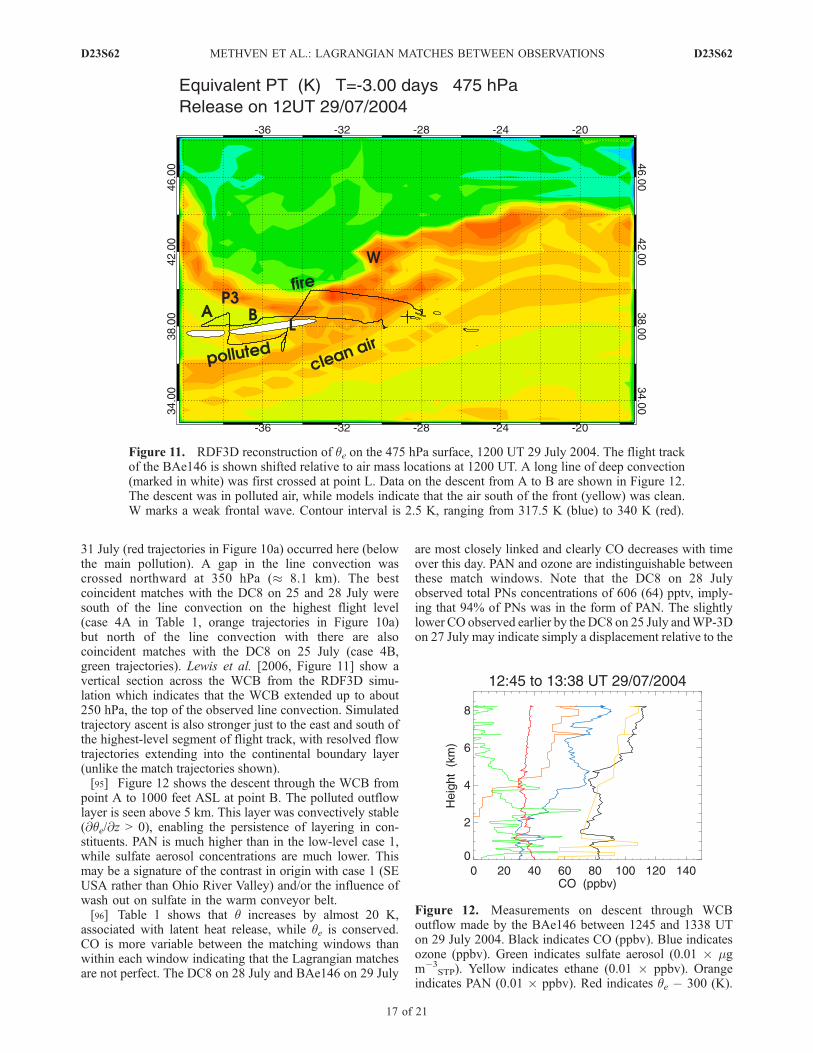
31 July (red trajectories in Figure 10a) occurred here (belowthe main pollution). A gap in the line convection wascrossed northward at 350 hPa (� 8.1 km). The bestcoincident matches with the DC8 on 25 and 28 July weresouth of the line convection on the highest flight level(case 4A in Table 1, orange trajectories in Figure 10a)but north of the line convection with there are alsocoincident matches with the DC8 on 25 July (case 4B,green trajectories). Lewis et al. [2006, Figure 11] show avertical section across the WCB from the RDF3D simu-lation which indicates that the WCB extended up to about250 hPa, the top of the observed line convection. Simulatedtrajectory ascent is also stronger just to the east and south ofthe highest-level segment of flight track, with resolved flowtrajectories extending into the continental boundary layer(unlike the match trajectories shown).[95] Figure 12 shows the descent through the WCB from

point A to 1000 feet ASL at point B. The polluted outflowlayer is seen above 5 km. This layer was convectively stable(@qe/@z > 0), enabling the persistence of layering in con-stituents. PAN is much higher than in the low-level case 1,while sulfate aerosol concentrations are much lower. Thismay be a signature of the contrast in origin with case 1 (SEUSA rather than Ohio River Valley) and/or the influence ofwash out on sulfate in the warm conveyor belt.[96] Table 1 shows that q increases by almost 20 K,

associated with latent heat release, while qe is conserved.CO is more variable between the matching windows thanwithin each window indicating that the Lagrangian matchesare not perfect. The DC8 on 28 July and BAe146 on 29 July

are most closely linked and clearly CO decreases with timeover this day. PAN and ozone are indistinguishable betweenthese match windows. Note that the DC8 on 28 Julyobserved total PNs concentrations of 606 (64) pptv, imply-ing that 94% of PNs was in the form of PAN. The slightlylower CO observed earlier by the DC8 on 25 July andWP-3Don 27 July may indicate simply a displacement relative to the

Figure 11. RDF3D reconstruction of qe on the 475 hPa surface, 1200 UT 29 July 2004. The flight trackof the BAe146 is shown shifted relative to air mass locations at 1200 UT. A long line of deep convection(marked in white) was first crossed at point L. Data on the descent from A to B are shown in Figure 12.The descent was in polluted air, while models indicate that the air south of the front (yellow) was clean.W marks a weak frontal wave. Contour interval is 2.5 K, ranging from 317.5 K (blue) to 340 K (red).

Figure 12. Measurements on descent through WCBoutflow made by the BAe146 between 1245 and 1338 UTon 29 July 2004. Black indicates CO (ppbv). Blue indicatesozone (ppbv). Green indicates sulfate aerosol (0.01 � mgm�3

STP). Yellow indicates ethane (0.01 � ppbv). Orangeindicates PAN (0.01 � ppbv). Red indicates qe � 300 (K).


17 of 21

D23S62

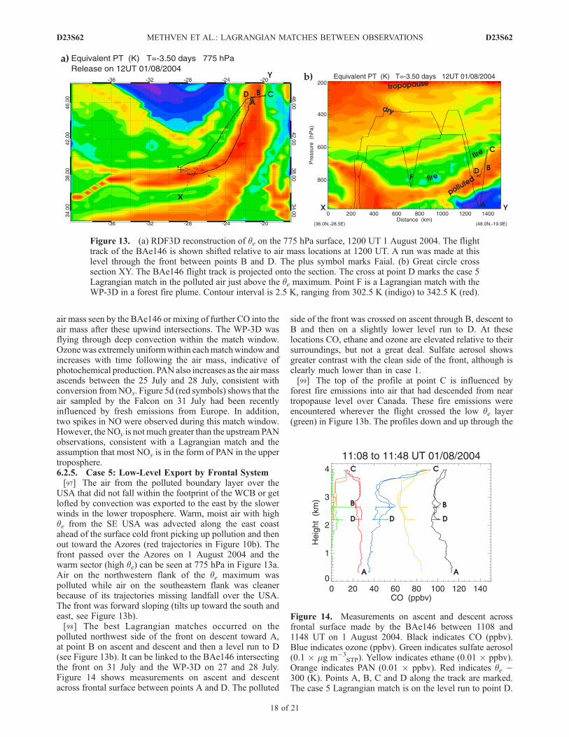
air mass seen by the BAe146 or mixing of further CO into theair mass after these upwind intersections. The WP-3D wasflying through deep convection within the match window.Ozonewas extremely uniformwithin eachmatchwindowandincreases with time following the air mass, indicative ofphotochemical production. PAN also increases as the air massascends between the 25 July and 28 July, consistent withconversion fromNOx. Figure 5d (red symbols) shows that theair sampled by the Falcon on 31 July had been recentlyinfluenced by fresh emissions from Europe. In addition,two spikes in NO were observed during this match window.However, the NOy is not much greater than the upstream PANobservations, consistent with a Lagrangian match and theassumption that most NOy is in the form of PAN in the uppertroposphere.6.2.5. Case 5: Low-Level Export by Frontal System[97] The air from the polluted boundary layer over the

USA that did not fall within the footprint of the WCB or getlofted by convection was exported to the east by the slowerwinds in the lower troposphere. Warm, moist air with highqe from the SE USA was advected along the east coastahead of the surface cold front picking up pollution and thenout toward the Azores (red trajectories in Figure 10b). Thefront passed over the Azores on 1 August 2004 and thewarm sector (high qe) can be seen at 775 hPa in Figure 13a.Air on the northwestern flank of the qe maximum waspolluted while air on the southeastern flank was cleanerbecause of its trajectories missing landfall over the USA.The front was forward sloping (tilts up toward the south andeast, see Figure 13b).[98] The best Lagrangian matches occurred on the

polluted northwest side of the front on descent toward A,at point B on ascent and descent and then a level run to D(see Figure 13b). It can be linked to the BAe146 intersectingthe front on 31 July and the WP-3D on 27 and 28 July.Figure 14 shows measurements on ascent and descentacross frontal surface between points A and D. The polluted

side of the front was crossed on ascent through B, descent toB and then on a slightly lower level run to D. At theselocations CO, ethane and ozone are elevated relative to theirsurroundings, but not a great deal. Sulfate aerosol showsgreater contrast with the clean side of the front, although isclearly much lower than in case 1.[99] The top of the profile at point C is influenced by

forest fire emissions into air that had descended from neartropopause level over Canada. These fire emissions wereencountered wherever the flight crossed the low qe layer(green) in Figure 13b. The profiles down and up through the

Figure 13. (a) RDF3D reconstruction of qe on the 775 hPa surface, 1200 UT 1 August 2004. The flighttrack of the BAe146 is shown shifted relative to air mass locations at 1200 UT. A run was made at thislevel through the front between points B and D. The plus symbol marks Faial. (b) Great circle crosssection XY. The BAe146 flight track is projected onto the section. The cross at point D marks the case 5Lagrangian match in the polluted air just above the qe maximum. Point F is a Lagrangian match with theWP-3D in a forest fire plume. Contour interval is 2.5 K, ranging from 302.5 K (indigo) to 342.5 K (red).

Figure 14. Measurements on ascent and descent acrossfrontal surface made by the BAe146 between 1108 and1148 UT on 1 August 2004. Black indicates CO (ppbv).Blue indicates ozone (ppbv). Green indicates sulfate aerosol(0.1 � mg m�3

STP). Yellow indicates ethane (0.01 � ppbv).Orange indicates PAN (0.01 � ppbv). Red indicates qe �300 (K). Points A, B, C and D along the track are marked.The case 5 Lagrangian match is on the level run to point D.


18 of 21

D23S62

fire layer near F revealed that CO was highest near thebottom of the layer (150 ppbv) but near the top there was adry layer with higher ozone. Very similar characteristicswere observed by the BAe146 on 31 July: At this earliertime the top layer contained ozone up to 200 ppbv, implyingthat the fire emissions had mixed with stratospheric air.Point F also has coincident matches with the WP-3D on28 July when it intercepted the fire plume north of theSt. Lawrence River (yellow trajectories in Figure 10b).[100] In case 5, q decreases slowly with time and qe

decreases at a faster rate. This could be explained by mixingbetween the high qe of the polluted air mass and the verylow qe of the cold, dry layer immediately above the frontalsurface (see Figure 13b). CO barely changes with time sincethe CO contrast between the two air masses is very weak(Figure 14). An increase in benzene/ethane ratio (a charac-teristic of fire plume case 2) between 31 July and 1 Augustsupports the hypothesis of mixing with the fire layer. PANdecreases with time associated with thermal decomposition.Ozone decreases with time, but modeling studies arerequired to determine the contribution from photochemicalloss.

7. Conclusions

[101] Evidence has been presented to demonstrate that airmasses were sampled several times during transit across theNorth Atlantic as part of the ITCT-Lagrangian-2K4 exper-iment. Many Lagrangian matches were identified objectivelyusing a novel technique that combines Lagrangian trajecto-ries, calculated using global meteorological analyses, and thehydrocarbon fingerprints analyzed from whole air samplescollected by the aircraft. Five cases were identified withstrong links between at least three flights spanning theAtlantic. The variability between the hydrocarbon finger-prints of linked samples is very small compared to thedifferences between randomly selected samples, once theloss of hydrocarbons through OH reaction over the timebetween samples is accounted for. The relationships betweenthe longer-lived hydrocarbons are particularly close, withvariability comparable to the variability between samplescollected on one flight through the same air mass.[102] There is always uncertainty concerning the close-

ness of the Lagrangian matches. The ideal situation wouldbe for the differences between downwind and upwindinterceptions of an air mass to reveal photochemical trans-formation in composition. However, two factors render thistask difficult:[103] 1. Variability within an air mass, since the upwind

and downwind aircraft may sample the air mass differently,even if its structure and composition had not changed overthe interval between flights. For example, in case 2, fol-lowing the Alaskan fire plume, there was strong variabilityin CO and the DC8 and BAe146 spent a different fraction oftime near the CO maximum. There is also uncertainty in thevertical structure of the plume and the level of the aircraftrelative to the plume maximum. However, other tracers, thatare not directly emitted from the fires, are much moreuniform. For example, equivalent potential temperatureagrees to within 1 K between the interceptions of theDC8, BAe146 and Falcon through the plume. Since ozonevariability is small within the plume it is reasonable to

suggest that the downwind minus upwind differences are agood estimate of ozone evolution.[104] 2. Mixing by turbulence following the flow resolved

in atmospheric analyses. In the Lagrangian experiment, therate of mixing was not observed between interceptions andthe gradients with neighboring air masses, which changecontinuously, were also not sampled between flights. Theonly quantitative way to partition the observed changebetween photochemical reaction and physical processes isthrough the use of a model.[105] Bearing these limitations in mind, the quality of

different matching techniques was assessed using indepen-dent observations of tracers to find downwind minusupwind differences. The distribution of qe differences fortrajectory-only or hydrocarbon-only matches was muchmore strongly peaked about zero than pairing random timepoints drawn from the same set of flights. Importantly, whenthe information was combined in the search for ‘‘coincidentmatches’’ the peak of the PDF more than doubled, showingthat the quality of these matches was much higher. With theexception of the coincident trajectories in case 3, the qedifferences almost all lie within �3 to +1 K day�1,consistent with pseudoadiabatic evolution following airmasses. Potential temperature increase shows that some ofthese coincident matches experienced latent heat releaseassociated with ascent and condensation. In addition, thePDFs were very similar when using the UGAMP trajectorymodel or FLEXPART Lagrangian dispersion model,together with hydrocarbon fingerprints, to identify matches.This indicates that the quality of the matches identifiedusing two different models, with different trajectorymatchingcriteria, are similar even though there are differences in thematch windows highlighted.[106] The PDF of CO growth rate (defined by (3)) shows

CO increase for a few matches, either indicating a mismatchor mixing of more CO into the air mass. However, in thevast majority of cases there is slow CO decrease with anassociated timescale of greater than 10 days for 73% ofmatches. The CO decreases more slowly than the timescaleof turbulent mixing because the targets do not have muchhigher CO than their surroundings (except in the Alaskanfire plume case 2).[107] The PDF of ozone growth rate peaks at slow

increase. It is not possible to quantify the proportionassociated with photochemistry, as opposed to mixing,without running a photochemical model for all matches.[108] The best five Lagrangian cases (see Table 1) cover a

variety of situations. Cases 1, 3 and 5 followed anthropo-genic pollution at low levels from the east coast USA rightacross the Atlantic. Case 3 was clearly influenced byentrainment from a dry layer overlying the pollution (topat 850 hPa). Nevertheless, mixing was so slow that layeringand strong variability in CO was still observed by theFalcon just west of Ireland. Case 1 also retained a highlystratified structure with weak mixing and virtually no shearin the flow. Two distinct air masses were identified travelingone above the other, both characterized by very high sulfateaerosol concentrations. The upper layer (1A) traveled justabove the marine boundary layer and appeared to mix veryslowly with its neighbors, while the lower layer (1B)descended slowly into the marine boundary layer. Contin-uous, but slow, entrainment from the polluted low-level


19 of 21

D23S62

outflow helped to maintain high pollutant levels (e.g.,sulfate aerosol) in the marine BL below, as observed inLagrangian case 3 of ACE-2 [Wood et al., 2000]. Ozonedecrease occurred in air masses traveling at low level, evenif well above the boundary layer (e.g., case 5 following acold front). Case 2 followed a highly polluted plumeoriginating from fires in Alaska as it descended from theupper troposphere across the Atlantic. Case 4 followed airascending from southeast USA in a warm conveyor belt andthen across the Atlantic in the upper troposphere. Ozoneincrease occurs in the upper troposphere in anthropogenicpollution and the Alaskan fire plume.[109] The cases detailed in this paper provide a basis for

detailed chemical transport modeling studies constrained byobservations. It is hoped that changes in concentrations ofcompounds that are not routinely observed, such as higherhydrocarbons, OVOCs, alkyl nitrates and peroxy nitrateswill reveal exciting new information about photochemicalreaction pathways.

[110] Acknowledgments. Thanks to the whole of the ICARTT team:the scientists, pilots and support staff associated with all the measurementplatforms and their campaign bases. The Natural Environment ResearchCouncil (NERC) funded the ITOP-UK project and flying time as part of theUpper Troposphere – Lower Stratosphere Ozone (UTLS) thematicprogramme. The ITOP-UK team would also like to give heartfelt thanksto the dedication of the staff from the Facility for Airborne AtmosphericMeasurements and in particular, John Reid, without whom the BAe146would never have reached the Azores, let alone made measurements, on itsfirst deployment. The deployment of the DLR Falcon in Creil, France, wasfunded by DLR. French participation in European ITOP was funded byProgramme National de Chimie Atmospherique (PNCA) (ADEME, Agencegouvernementale de l’Environnement et de la Maitrise de l’energie)/PATOM (Programme Atmosphere et Ocean Multi-echelles) of INSU(Institut National des Sciences de l’Univers) and IPSL (Institut PierreSimon Laplace). Local support from IGN (Institut Geographique National),Creil, is gratefully acknowledged. Particular thanks to Tom B. Ryerson andGerd Hubler (NOAA Earth System Research Lab) for the WP-3D coremeasurements, Glen W. Sachse (NASA Langley RC) for the DC8 COmeasurements and Ron C. Cohen (UCI) for the DC8 total peroxynitratemeasurements. John Methven is grateful for support through an AdvancedFellowship jointly sponsored by NERC and the Environment Agency.

ReferencesBates, T., B. Huebert, J. Gras, F. Griffiths, and P. Durkee (1998), Interna-tional Global Atmospheric Chemistry (IGAC) Project’s first AerosolCharacterisation Experiment (ACE-1): Overview, J. Geophys. Res.,103, 16,297–16,318.

Day, D. A., P. J. Wooldridge, M. B. Dillon, J. A. Thornton, and R. C. Cohen(2002), A thermal dissociation laser-induced fluorescence instrument forin situ detection of NO2, peroxy nitrates, alkyl nitrates, and HNO3,J. Geophys. Res., 107(D6), 4046, doi:10.1029/2001JD000779.

Derwent, R., P. Simmonds, S. Seuring, and C. Dimmer (1998), Observationand interpretation of the seasonal cycles in the surface concentrations ofozone and carbon monoxide at Mace Head, Ireland from 1990 to 1994,Atmos. Environ., 32, 145–157.

Eckhardt, S., A. Stohl, H. Wernli, P. James, C. Forster, and N. Spichtinger(2004), A 15-year climatology of warm conveyor belts, J. Clim., 17,218–237.

Esler, J., G. Roelofs, M. Kohler, and F. O’Connor (2004), A quantitativeanalysis of grid-related systematic errors in oxidising capacity and ozoneproduction rates in chemistry transport models, Atmos. Chem. Phys., 4,1781–1795.

Fehsenfeld, F., et al. (2006), International Consortium for AtmosphericResearch on Transport and Transformation (ICARTT): North Americato Europe: Overview of the 2004 summer field study, J. Geophys. Res.,doi:10.1029/2006JD007829, in press.

Fitzgerald, J., J. Marti, W. Hoppel, G. Frick, and F. Gelbard (1998), A one-dimensional sectional model to simulate multicomponent aerosol dy-namics in the marine boundary layer: 2. Model application, J. Geophys.Res., 103, 16,103–16,117.

Forster, C., et al. (2001), Transport of boreal forest fire emissions fromCanada to Europe, J. Geophys. Res., 106, 22,887–22,906.

Frost, G. J., et al. (2006), Effects of changing power plant NOx emissionson ozone in the eastern United States: Proof of concept, J. Geophys. Res.,111, D12306, doi:10.1029/2005JD006354.

Guenther, A., et al. (1995), A global model of natural volatile organiccompound emissions, J. Geophys. Res., 100, 8873–8892.

Haynes, P., and J. Anglade (1997), The vertical-scale cascade in atmo-spheric tracers due to large-scale differential advection, J. Atmos. Sci.,54, 1121–1136.

Hoell, C., C. O’Dowd, S. Osborne, and D. Johnson (2000), Time-scaleanalysis of marine boundary layer aerosol evolution: Lagrangian casestudies under clean and polluted cloudy conditions, Tellus, Ser. B, 52,423–438.

Huebert, B., A. Pszenny, and B. Blomquist (1996), The ASTEX/MAGEexperiment, J. Geophys. Res., 101, 4319–4329.

Jobson, B., D. Parrish, P. Goldan, W. Kuster, F. Fehsenfeld, D. Blake,N. Blake, and H. Niki (1998), Spatial and temporal variability of non-methane hydrocarbon mixing ratios and their relation to photochemicallifetime, J. Geophys. Res., 103, 13,557–13,567.

Johnson, D., S. Osborne, R. Wood, K. Suhre, R. Johnson, and S. Businger(2000), An overview of the Lagrangian experiments undertaken duringthe North Atlantic regional Aerosol Characterization Experiment (ACE-2), Tellus, Ser. B, 52, 290–320.

Legras, B., B. Joseph, and F. Lefvre (2003), Vertical diffusivity in the lowerstratosphere from Lagrangian back-trajectory reconstructions of ozoneprofiles, J. Geophys. Res., 108(D18), 4562, doi:10.1029/2002JD003045.

Lehmann, R., P. von der Gathen, M. Rex, and M. Streibel (2005), Statisticalanalysis of the precision of the Match method, Atmos. Chem. Phys., 5,2713–2727.

Lewis, A., et al. (2006), Chemical composition observed over the mid-Atlantic and the detection of pollution signatures far from source regions,J. Geophys. Res., doi:10.1029/2006JD007584, in press.

Methven, J. (1997), Offline trajectories: Calculation and accuracy, Tech.Rep. 44, U. K. Univ. Global Atmos. Modell. Program, Dep. of Meteorol.,Univ. of Reading, Reading, U. K.

Methven, J., and B. Hoskins (1999), The advection of high resolutiontracers by low resolution winds, J. Atmos. Sci., 56, 3262–3285.

Methven, J., S. Arnold, F. O’Connor, H. Barjat, K. Dewey, J. Kent, andN. Brough (2003), Estimating photochemically produced ozone through-out a domain using flight data and a Lagrangian model, J. Geophys. Res.,108(D9), 4271, doi:10.1029/2002JD002955.

Olivier, J., A. Bouwman, J. Berdowski, C. Veldt, J. Bloos, A. Visschedijk,C. van der Maas, and P. Zandveld (1999), Sectoral emission inventoriesof greenhouse gases for 1 990 on a per country basis as well as on 1 � 1degree, Environ. Sci. Policy, 2, 241–264.

Parrish, D. (2006), The effects of mixing on evolution of hydrocarbon ratiosin the troposphere, J. Geophys. Res., doi:10.1029/2006JD007583, inpress.

Parrish, D., M. Trainer, J. Holloway, J. Yee, M. Warshawsky, F. Fehsenfeld,G. Forbes, and J. Moody (1998), Relationships between ozone and car-bon monoxide at surface sites in the North Atlantic region, J. Geophys.Res., 103(D11), 13,357–13,376.

Pfister, G., P. Hess, L. Emmons, J.-F. Lamarque, C.Wiedinmyer, D. Edwards,G. Petron, J. Gille, and G. Sachse (2005), Quantifying CO emissions fromthe 2004 Alaskan wildfires using MOPITT CO data, Geophys. Res. Lett.,32, L11809, doi:10.1029/2005GL022995.

Prinn, R., R. Weiss, B. Miller, J. Huang, F. Alyea, D. Cunnold, P. Fraser,D. Hartley, and P. Simmonds (1995), Atmospheric trends and lifetimeof CH3CCl3 and global OH concentrations, Science, 269, 187–192.

Raes, F., T. Bates, F. McGovern, and M. van Leide (2000), The secondAerosol Characterisation Experiment (ACE-2): General overview andmain results, Tellus, Ser. B, 52, 111–125.

Real, E., et al. (2006), Processes influencing ozone levels in Alaskan forestfires plumes during long-range transport over the North Atlantic, J. Geo-phys. Res., doi:10.1029/2006JD007576, in press.

Rex, M., et al. (1998), In situ measurements of stratospheric ozone depletionrates in the Arctic winter 1991/ 1992: A Lagrangian approach, J. Geophys.Res., 103(D5), 5843–5854.

Riddle, E., P. Voss, A. Stohl, D. Holcomb, D. Mazcka, K. Washburn, andR. Talbot (2006), Trajectory model validation during the InternationalConsortium for Atmospheric Research on Transport and Transforma-tions 2004 using newly developed altitude-controlled meteorologicalballoons, J. Geophys. Res., 111, D23S57, doi:10.1029/2006JD007456.

Stohl, A., S. Eckhardt, C. Forster, P. James, N. Spichtinger, and P. Seibert(2002), A replacement for simple back trajectory calculations in theinterpretation of atmospheric trace substance measurements, Atmos.Environ., 36, 4635–4648.

Stohl, A., et al. (2003), A backward modeling study of intercontinentalpollution transport using aircraft measurements, J. Geophys. Res.,108(D12), 4370, doi:10.1029/2002JD002862.


20 of 21

D23S62

Stohl, A., O. Cooper, R. Damoah, F. Fehsenfeld, C. Forster, E.-Y. Hsie,G. Hubler, D. Parrish, andM. Trainer (2004), Forecasting for a Lagrangianaircraft campaign, Atmos. Chem. Phys., 4, 1113–1124.

Stohl, A., C. Forster, A. Frank, P. Seibert, and G. Wotawa (2005), TheLagrangian particle dispersion model FLEXPART version 6.2, Atmos.Chem. Phys., 5, 2461–2474.

Wood, R., et al. (2000), Boundary layer and aerosol evolution during the3rd Lagrangian experiment of ACE-2, Tellus, Ser. B, 52, 401–422.

��S. R. Arnold, M. J. Evans, and J. McQuaid, School of Earth and

Environment, University of Leeds, Leeds LS2 9JT, UK.E. Atlas, Rosenstiel School of Marine and Atmospheric Science,

University of Miami, Miami, FL 33149-1098, USA.M. Avery, NASA Langley Research Center, Hampton, VA 23681, USA.D. R. Blake, Department of Chemistry, University of California, Irvine,

CA 92697, USA.H. Coe, J. Crosier, and P. I. Williams, School of Earth, Atmospheric and

Environmental Sciences, University of Manchester, Manchester M13 9PL,UK.F. M. Flocke, Atmospheric Chemistry Division, National Center for

Atmospheric Research, Boulder, CO 80305, USA.

J. S. Holloway and D. D. Parrish, Earth System Research Laboratory,NOAA, Boulder, CO 80305, USA.J. R. Hopkins, A. C. Lewis, and N. M. Watson, Department of Chemistry,

University of York, York YO10 5DD, UK.K. Law, Service d’Aeronomie, Centre National de la Recherche

Scientifique, Universite Pierre et Marie Curie, F-75252 Paris, France.J. Methven, Department of Meteorology, University of Reading, P.O.

Box 243, Earley Gate, Reading RG6 6BB, UK. ([email protected])P. S. Monks, Department of Chemistry, University of Leicester, Leicester

LE1 7RH, UK.R. Purvis, Facility for Airborne Atmospheric Measurements, Cranfield

MK43 0AL, UK.B. Rappengluck, Institute of Meteorology and Climate Research,

ForschungszentrumKarlsruhe, D-82467 Garmisch-Partenkirchen, Germany.C. E. Reeves, School of Environmental Sciences, University of East

Anglia, Norwich NR4 7TJ, UK.H. Schlager, Deutsches Zentrum fur Luft- und Raumfahrt, D-82230

Oberpfaffenhofen, Germany.H. B. Singh, NASA Ames Research Center, Moffett Field, CA 94035,

USA.A. Stohl, Norwegian Institute for Air Research, N-2027 Kjeller, Norway.L. K. Whalley, School of Chemistry, University of Leeds, Leeds LS2 9JT,

UK.


21 of 21

D23S62

Establishing Lagrangian connections between observations within air masses crossing the Atlantic during the International Consortium for Atmospheric Research on Transport and Transformation

Documents