error bounds for polynomial and spline interpolation

ERROR BOUNDS FOR POLYNOMIAL AND SPLINE INTERPOLATION

By

GARY WILBUR HOWELL

A DISSERTATION PRESENTED TO THE GRADUATE SCHOOL OF THE UNIVERSITY OF FLORIDA IN

PARTIAL FULFILLMENT OF THE REQUIREMENTS FOR THE DEGREE OF DOCTOR OF PHILOSOPHY

UNIVERSITY OF FLORIDA

1986

Copyright 1986

by

Gary Wilbur Howell

To my wife, Nadia

ACKNOWLEDGEMENTS

I wish to express my sincerest appreciation to Dr.

Arun Varma for his research counseling and assistance

throughout my graduate school years. I wish also to thank

Ors. David Drake, Nicolae Dinculeanu, and Soo Bong Chae,

for their teaching and for encouraging me to pursue the

doctorate in mathematics, as well as Ors. Vasile Popov and

A. I. Khuri for their kindness in serving on my committee.

Finally of course, my parents and wife deserve rather more

thanks than can be easily expressed.

iv

TABLE OF CONTENTS

ACKNOWLEDGEMENTS •

ABSTRACT

CHAPTER

ONE

TWO

THREE

FOUR

INTRODUCTION

Lagrange and Hermite-Fejer Interpolation

Optimal Error Bounds for Two Point Hermite Interpolation

Birkhoff Interpolation Polynomial Approximation. Spline Approximation Parabolic Spline Interpolation • Optimal Error Bounds for Cubic

Spline Interpolation

BEST ERROR BOUNDS FOR DERIVATIVES OF TWO POINT LIDSTONE POLYNOMIALS

Introduction and Statement of Main Theorem

Preliminaries Proof of Theorem 3.1

A QUARTIC SPLINE

Introduction and Statement Theorems

Proof of Theorem 3.1

A QUARTIC SPLINE

Introduction and Statement Theorems

Proof of Lemma 4.1 . Proof of Theorem 4.1 Proof of Theorem 4.2

V

of

of

iv

vii

1

2

4 8

13 16 25

27

30

30 33 37

43

43 54

60

60 66 69 78

FIVE

SIX

IMPROVED ERROR BOUNDS FOR THE PARABOLIC SPLINE .

Introduction and Statement of Theorems

Proof of Theorem 5.1 Proof of Theorem 5.2 Proof of Theorem 5.3

CONCLUDING REMARKS

REFERENCES

BIOGRAPHICAL SKETCH

vi

81

85 85 88 98

107

110

113

Abstract of Dissertation Presented to the Graduate School of the University of Florida in Partial Fulfillment of the

Requirements for the Degree of Doctor of Philosophy

ERROR BOUNDS FOR POLYNOMIAL AND SPLINE INTERPOLATION

By

Gary Wilbur Howell

August 1986

Chairman: Dr. Arun K. Varma Major Department: Department of Mathematics

The present dissertation is motivated by a desire to

have a more precise knowledge of asymptotic approximation

error than that given by best order of approximation. It

owes its inspiration to a paper by G. Birkhoff and A. Priver

concerning error bounds for derivatives of Hermite

interpolation and a paper of C. A. Hall and w. W. Meyer

concerning error bounds for cubic splines.

In Chapter One we consider well known results

concerning interpolation, polynomial approximation and

error analysis of spline approximation. The results given

here are meant to provide a context for the theorems given

in later chapters. In Chapters Two and Three we consider

the problem of best error bounds for derivatives in two

point Birkhoff interpolation problems.

vii

Chapter Four presents the problems of existence,

uniqueness, explicit representation, and the problem of

convergence for fourth degree splines. Moreover we also

consider the problem of optimal pointwise error bounds for

functions f e c(S) [0,1). In Chapter Five our main object

is to sharpen the error bounds obtained earlier by Marsden

concerning quadratic spline interpolation. By doing so we

obtain in some special cases error bounds that are in fact

optimal.

viii

CHAPTER ONE INTRODUCTION

The purpose of this chapter is to provide a context

for the results derived in succeeding chapters. In order

to show some of the important achievements in

approximation by polynomials, we discuss briefly the

Lagrange and Hermite-Fejer interpolations, which match a

given function at any finite number of distinct points.

After exploring the question of computational stability of

a given interpolation, we discuss in some detail the

problem of best order of approximation by polynomials as

initiated by S. N. Bernstein [1912], D. Jackson [1930],

and A. Zygmund [1968].

In contrast to high order approximation by a single

polynomial, we next consider in great detail the problem

of approximating a given function f(x) defined on [a,b]

by the interpolatory piecewise polynomials known as

splines. Special attention is given to the problem of

approximating by piecewise cubic and piecewise parabolic

splines. The study of these splines motivates us to also

study two point Hermite and Birkhoff interpolations.

1

2

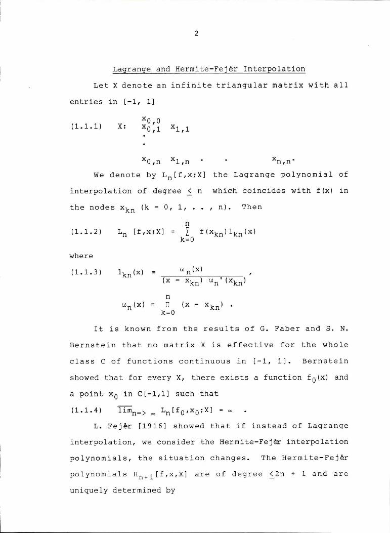
Lagrange and Hermite-Fejer Interpolation

Let X denote an infinite triangular matrix with all

entries in [-1, 1]

(1.1.1) X:

We denote by Ln[f,x;X] the Lagrange polynomial of

interpolation of degree~ n which coincides with f(x) in

the nodes xkn ( k = 0, 1, . • , n). Then

(1.1.2)

where

(1.1.3)

Ln [ f, x; X] =

=

n

n L f(xknl 1kn(x)

k=O

wn(x)

wn(x) = IT (x - xkn) • k=O

It is known from the results of G. Faber and S. N.

Bernstein that no matrix Xis effective for the whole

class C of functions continuous in [-1, 1). Bernstein

showed that for every X, there exists a function f 0 (x) and

a point x 0 in C[-1,1] such that

(1.1.4)

L. Fejer [1916) showed that if instead of Lagrange

interpolation, we consider the Hermite-Fejer interpolation

polynomials, the situation changes. The Hermite-Fejer

polynomials Hn+l[f,x,X] are of degree < 2n + 1 and are

uniquely determined by

3

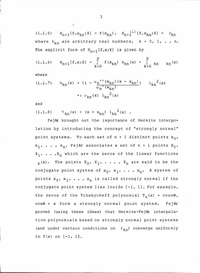
(1.1.5)

where okn are arbitrary real numbers, k = 0, 1, .• n.

The explicit form of Hn+l[f,x;X] is given by

(1.1.6)

where

(1.1. 7)

and

(1.1.8)

Hn + l [ f , x ; X] =

= ( 1 - w n' ' ( xkn) ( x - xkn) } wn' (xkn)

- • v kn ( x) 1 kn 2 ( x)

n kn ( x) = ( x - xkn) 2 lkn (x) •

2 lkn (x)

kn(x)

Fej& brought out the importance of Hermite interpo­

lation by introducing the concept of "strongly normal"

point systems. To each set of n + 1 distinct points x 0 ,

x 1 , .• , xn, Fejer associates a set of n + 1 points x 0 ,

x 1 , ,Xn which are the zeros of the linear functions

, Xn are said to be the

conjugate point system of x 0 , x 1 , , xn. A system of

points x 0 , x 1 , •• , xn is called strongly normal if the

conjugate point system lies inside [-1, 1]. For example,

the zeros of the Tchebycheff polynomial Tn(x) = cosne,

case= x form a strongly normal point system. Fejer

proved (using these ideas) that Hermite-Fej& interpola­

tion polynomials based on strongly normal point systems

(and under certain conditions on okn) converge uniformly

to f(x) on [-1, 1].

4

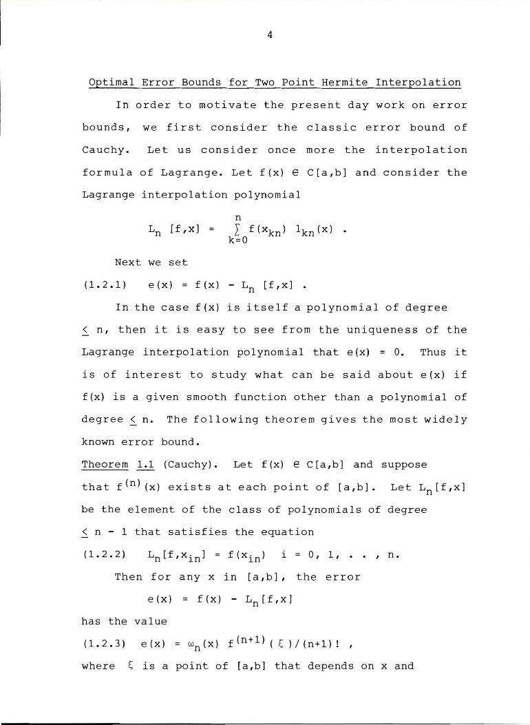
Optimal Error Bounds for Two Point Hermite Interpolation

In order to motivate the present day work on error

bounds, we first consider the classic error bound of

Cauchy. Let us consider once more the interpolation

formula of Lagrange. Let f(x) e C[a,b] and consider the

Lagrange interpolation polynomial

Ln [ f ,x] =

Next we set

n I f(xkn) 1kn(x)

k=O

(1.2.1) e ( X) = f ( X) - Ln [ f 'X] •

In the case f(x) is itself a polynomial of degree

~ n, then it is easy to see from the uniqueness of the

Lagrange interpolation polynomial that e(x) = O. Thus it

is of interest to study what can be said about e(x) if

f(x) is a given smooth function other than a polynomial of

degree ~ n. The following theorem gives the most widely

known error bound.

Theorem 1.1 (Cauchy). Let f(x) e C[a,b] and suppose

that f(n) (x) exists at each point of [a,b]. Let Ln[f,x]

be the element of the class of polynomials of degree

< n - 1 that satisfies the equation

(1.2.2)

Then for any x in [a,b], the error

e ( X) = f ( X) - Ln [ f 'X]

has the value

( 1. 2 • 3 ) e ( x) = wn ( x) f ( n + 1 ) ( t_; ) / ( n + 1 ) ! ,

where t_; is a point of [a,b] that depends on x and

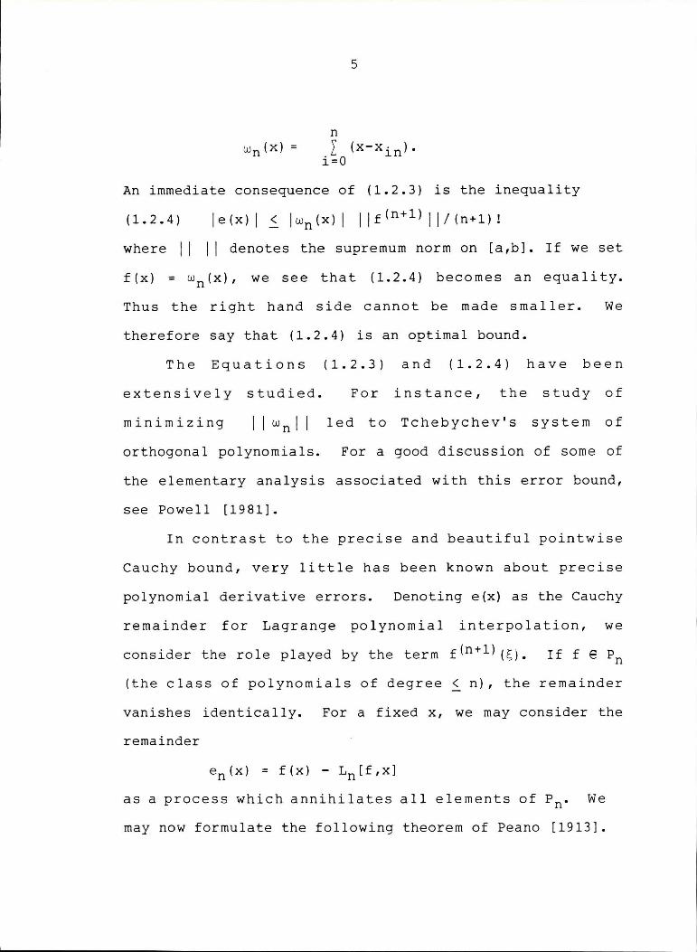
wn (x) =

5

n L (x-xin) •

i=O

An immediate consequence of (1.2.3) is the inequality

(1.2.4) I e ( x) I .S. I wn ( x) I I I f ( n + 1 ) I I / ( n + 1) !

where 11 11 denotes the supremurn norm on [a,b]. If we set

f(x) = wn(x), we see that (1.2.4) becomes an equality.

Thus the right hand side cannot be made smaller. We

therefore say that (1.2.4) is an optimal bound.

The Equations (1.2.3) and (1.2.4) have been

extensively studied. For instance, the study of

minimizing 11 wn 11 led to Tchebychev' s system of

orthogonal polynomials. For a good discussion of some of

the elementary analysis associated with this error bound,

see Powell [1981].

In contrast to the precise and beautiful pointwise

Cauchy bound, very little has been known about precise

polynomial derivative errors. Denoting e(x) as the Cauchy

remainder for Lagrange polynomial interpolation, we

consider the role played by the term f(n+l) (~i- If f e Pn

(the class of polynomials of degree~ n), the remainder

vanishes identically. For a fixed x, we may consider the

remainder

en ( X) = f ( X) - Ln [ f, X]

as a process which annihilates all elements of Pn. We

may now formulate the following theorem of Peano [1913].

6

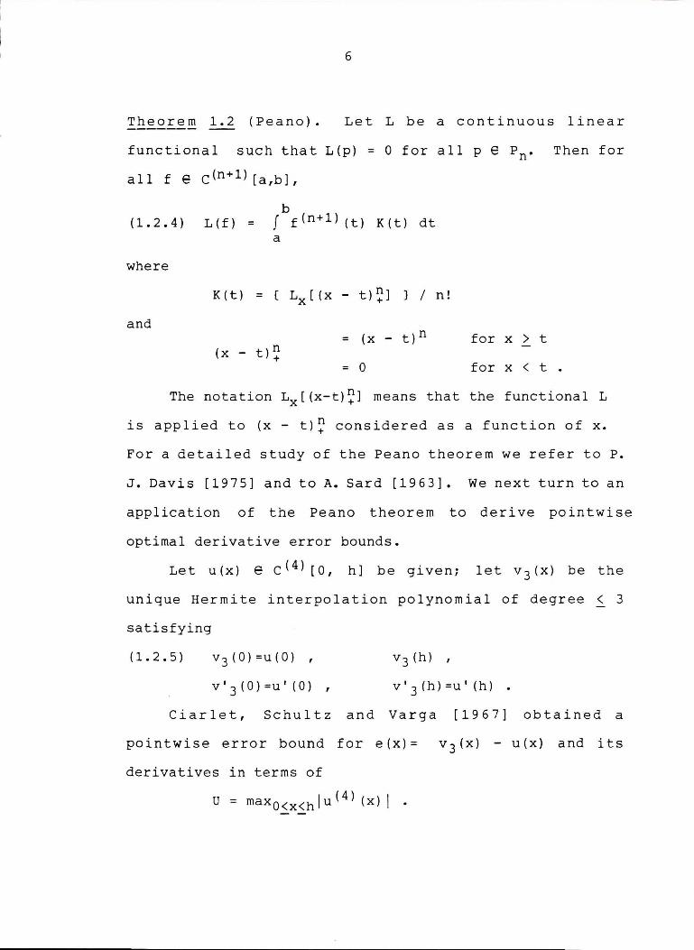
Theorem 1.2 (Peano). Let L be a continuous linear

functional such that L(p) = 0 for

all f e

(1.2.4)

where

and

c(n+l) [a,b],

b L(f) = f

a

K(t) = (

(x - t)~

f(n+l) (t) K (t) dt

LX [ (X - t)~] } I

= (X - t)n

= 0

all

n!

P e Pn.

for x > t

for x < t

Then for

The notation Lx[(x-t)~] means that the functional L

is applied to (x - t)~ considered as a function of x.

For a detailed study of the Peano theorem we refer to P.

J. Davis [1975] and to A. Sard [1963]. We next turn to an

application of the Peano theorem to derive pointwise

optimal derivative error bounds.

Let u(x) e c( 4 ) [O, h] be given; let v 3 (x) be the

unique Hermite interpolation polynomial of degree< 3

satisfying

(1.2.5) v 3 (0) =u(O) ,

v 1

3 (0)=u'(O),

v 3 (h) ,

v' 3 (h) =u' (h) .

Ciarlet, Schultz and Varga [1967] obtained a

pointwise error bound for e(x)= v 3 (x) - u(x) and its

derivatives in terms of

U = maxO<x<hlu (4 ) (x) I

7

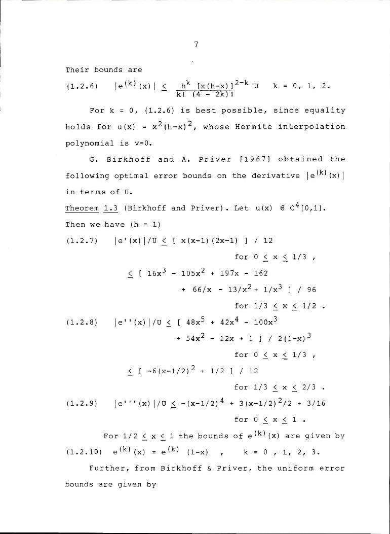
Their bounds are

(1.2.6) le(k) (x) I < hk [x(h-x)] 2-k U k ! ( 4 - 2k) !

k = 0, 1, 2.

Fork = 0, (1.2.6) is best possible, since equality

holds for u(x) = x 2 (h-x) 2 , whose Hermite interpolation

polynomial is v=O.

G. Birkhoff and A. Priver [1967] obtained the

following optimal error bounds on the derivative le(k) (x) I

in terms of U.

Theorem 1. 3 ( Birkhoff and Pri ver) . Let u (x) e c4 [ 0, 1].

Then we have (h = 1)

(1.2. 7)

(1.2.8)

(1.2.9)

le' (x) I/U .s_ x(x-1) (2x-1) ] / 12

for O < x < 1/3 ,

< [ 16x3 - 10Sx2 + 197x - 162

le' 1 (x) I/U <

+ 66/x - 13/x2 + l/x3 ] / 96

for 1/3 .s_ x < 1/2 .

48x 5 + 42x 4 - 100x3

+ 54x 2 - 12x + 1] / 2(1-x) 3

for O < x < 1/3 ,

< [ -6 ( x-1 / 2 l 2 + 1 / 2 J / 12

for 1/3 < x < 2/3 . - -

I e 1 ' ' ( x) I / U < - ( x-1 / 2) 4 + 3 ( x-1 / 2) 2 / 2 + 3 / 16

for O < x < 1 •

For 1/2 ~ x < 1 the bounds of e(k) (x) are given by

( 1. 2. 10) e ( k) ( x) = e ( k) ( 1-x) k = 0 , 1, 2, 3.

Further, from Birkhoff & Priver, the uniform error

bounds are given by

le (r) (x) < ar

(1.2.11)

8

u r = 1' 2'

ao = 1

4 2 4!

al = (/3)/216

a 2 = 1/12

a 3 = 1/2 •

3 '

The proof of the above theorem is based on the Peano

kernel theorem. It gives a general and highly useful

method for expressing the errors of approximations in

terms of derivatives of the underlying functions of the

approximation. For a computer routine which gives

polynomial error bounds by numerical quadrature of the

Peano kernel, see Howell and Diaa [1986]. Stroud [1974]

gives a readable account of some other applications.

Birkhoff Interpolation

We have just observed that in problems of Hermite

interpolation, function values and consecutive derivatives

are prescribed for given points. In 1906, G. D. Birkhoff

considered those interpolation problems in which the

consecutive derivative requirement can be dropped. This

more general kind of interpolation is now referred to as

the Birkhoff (or the lacunary) interpolation problem(s).

The Birkhoff interpolation problem differs from the

more familiar Lagrange and Hermite interpolation in both

its problems and its methods. For example, Lagrange and

Hermite interpolation problems are always uniquel y

9

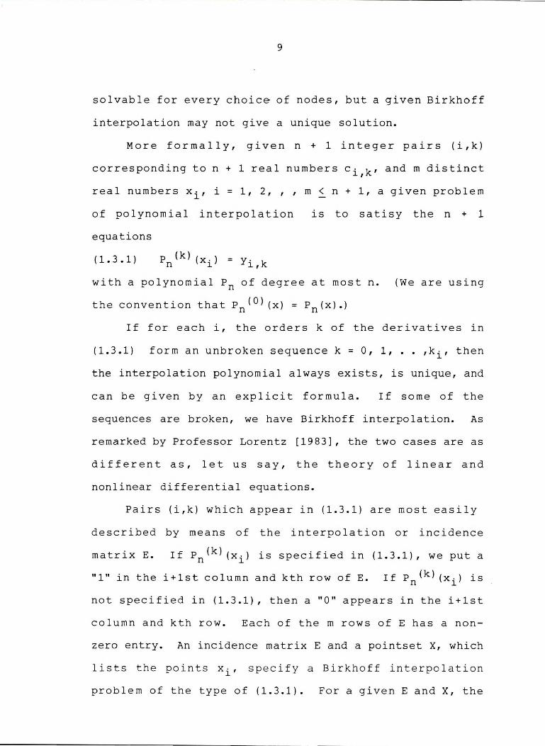
solvable for every choice of nodes, but a given Birkhoff

interpolation may not give a unique solution.

More formally, given n + 1 integer pairs (i,k)

corresponding ton+ 1 real numbers ci,k' and m distinct

real numbers xi, i = 1, 2, , , m < n + 1, a given problem

of polynomial interpolation

equations

is to satisy the n + 1

(1.3.1) p (k) (X·) = Y· k n l l,

with a polynomial Pn of degree at most n. (We are using

the convention that Pn (O) (x) = Pn (x) .)

If for each i, the orders k of the derivatives in

(1.3.1) form an unbroken sequence k = O, 1, •• ,ki' then

the interpolation polynomial always exists, is unique, and

can be given by an explicit formula. If some of the

sequences are broken, we have Birkhoff interpolation. As

remarked by Professor Lorentz [1983], the two cases are as

different as, let us say, the theory of linear and

nonlinear differential equations.

Pairs (i,k) which appear in (1.3.1) are most easily

described by means of the interpolation or incidence

matrix E. If pn(k) (xi) is specified in (1.3.1), we put a

"l" in the i+lst column and kth row of E. If P (k)(X·) is n l

not specified in (1.3.1), then a "O" appears in the i+lst

column and kth row. Each of them rows of E has a non­

zero entry. An incidence matrix E and a pointset X, which

lists the points x i, sp e cif y a Birkhoff interpolation

problem of the type of (1.3.1). For a given E and X, the

10

unique existence of an interpolation polynomial of degree

n + 1 is equivalent to the invertibility of the system of

equations given by (1.3.1), or equivalently to the inver­

tibi li ty of a matrix V which we will refer to as a

generalized Vandermonde matrix V. For Lagrange

interpolation of the points xi, i = 1, 2, •• , n + 1,

the Vandermonde Vis given as

1 1 1

(1.3.2) V =

X n 1

Inversion of the Vandermonde gives the coefficients of the

fundamental functions lkn(x) of Lagrange interpolation.

As Lagrange interpolations are always unique, it follows

that Vandermonde matrices are invertible.

For a given system (1.3.1), it is not hard to

construct an analagous matrix to (1.3.2), which we will

refer to as the generalized Vandermonde. Just as

inverting the Vandermonde matrix gives the fundamental

functions of Lagrange interpolation, inverting the genera­

lized Vandermonde gives a convenient form for representing

a Birkhoff interpolation. The Vandermonde and its

counterpart for Birkhoff interpolation are examples of

Gram matrices, of which a good account is to be found in

Davis [1975].

Though invertible, the Vandermonde matrices are known

to be extremely ill-conditioned for real-valued

11

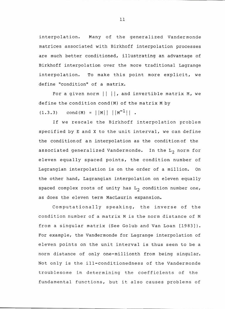
interpolation. Many of the generalized Vandermonde

matrices associated with Birkhoff interpolation processes

are much better conditioned, illustrating an advantage of

Birkhoff interpolation over the more traditional Lagrange

interpolation. To make this point more explicit, we

define "condition" of a matrix.

For a given norm 11 11, and invertible matrix M, we

define the condition cond(M) of the matrix M by

(1.3.3) cond (M) = I IM I I I I M-111 .

If we rescale the Birkhoff interpolation problem

specified by E and X to the unit interval, we can define

the condition of an interpolation as the condition of the

associated generalized Vandermonde. In the L 2 norm for

eleven equally spaced points, the condition number of

Lagrangian interpolation is on the order of a million. On

the other hand, Lagrangian interpolation on eleven equally

spaced complex roots of unity has L2 condition number one,

as does the eleven term MacLaurin expansion.

Computationally speaking, the inverse of the

condition number of a matrix Mis the norm distance of M

from a singular matrix (See Golub and Van Loan [1983]).

For example, the Vandermonde for Lagrange interpolation of

eleven points on the unit interval is thus seen to be a

norm distance of only one-millionth from being singular.

Not only is the ill-conditionedness of the Vandermonde

troublesome in determining the coefficients of the

fundamental functions, but it also causes problems of

12

round-off error in evaluating a polynomial by use of the

fundamental functions. For these reasons, it is very much

preferable to use a well-conditioned interpolation.

The MacLaurin expansion, having diagonal generalized

Vandermonde, is as well-conditioned as is possible.

Another particularly well-conditioned interpolation is the

Lidstone interpolation.

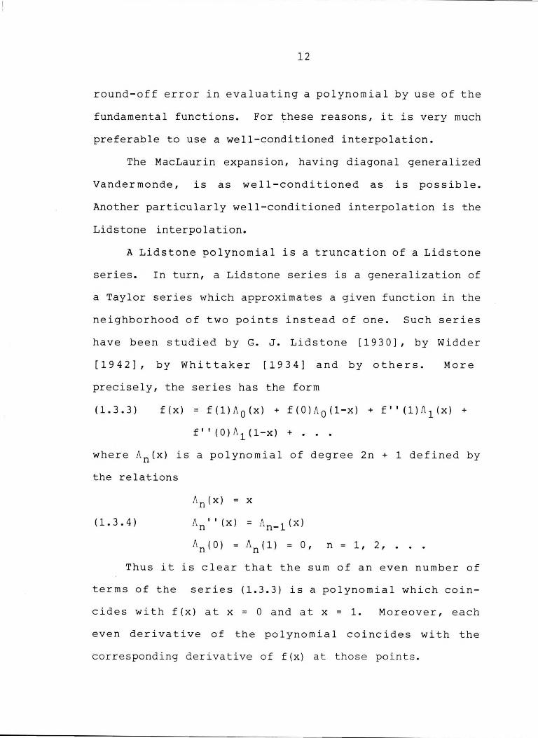
A Lidstone polynomial is a truncation of a Lidstone

series. In turn, a Lidstone series is a generalization of

a Taylor series which approximates a given function in the

neighborhood of two points instead of one. Such series

have been studied by G. J. Lidstone [1930], by Widder

[1942], by Whittaker [1934] and by others.

precisely, the series has the form

More

(1.3.3) f(x) = f(l)J\o(x) + f(0) J\ o(l-x) + f'' (l)J\1(X) +

f' ' ( 0) A 1 ( 1-x) + •

where J\n(x) is a polynomial of degree 2n + 1 defined by

the relations

J\ n(x) = x

(1.3.4) J\ n'' (x) = J\ n-1 (x)

J\n(0) = J\n(l) = 0, n = 1, 2, •..

Thus it is clear that the sum of an even number of

terms of the series (1.3.3) is a polynomial which coin-

cides with f(x) at x = 0 and at x = 1. Moreover, each

even derivative of the polynomial coincides with the

corresponding derivative of f(x} at those points.

13

Polynomial Approximation

Weierstrass first enunciated the theorem that an

arbitrary continuous function can be approximately

represented by a polynomial with any degree of accuracy.

We may express this theorem in the following form.

If f(x) is a given function, continuous for

a< x < b, and if E is a given positive quantity, it

is always possible to define a polynomial P(x) such that

(1.4.1) lf(x) - P(x) I < E

for all a< x < b.

It is readily seen that the number of terms required

to yield a specified degree of approximation, or under the

converse aspect, the degree of approximation attainable

with a specified number of terms, is related to the

properties of continuity of f(x). Naturally this has led

to many interesting developments in the theory of degree

of approximation of continuous functions by polynomials to

which we turn to describe.

A first important step in building this theory was

made by D. Jackson [1930]. Let f e C[-1,1]. Suppose that

we define the best approximation off by polynomials of

degree n by

(1.4.2)

where Pn ranges over all algebraic polynomials of degree n

and I lfl I = max lf(x) I, a~ x < b. Jackson considered the

problem of estimating En (f). To describe his results we

need the following definition.

14

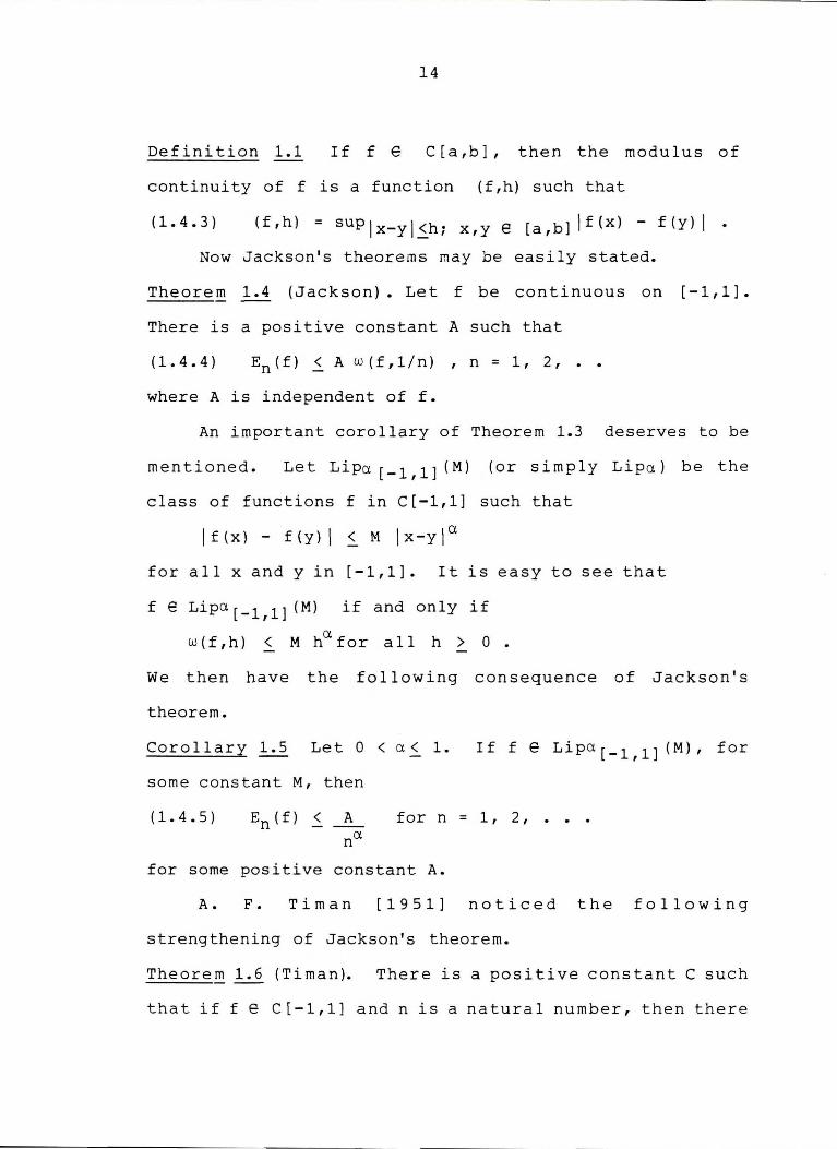
Definition 1.1 If f e C [a,b], then the modulus of

continuity of f is a function (f,h) such that

(1.4.3) (f,h) = suplx-y!~h; x,y e [a,b] If (x) - f(y) I .

Now Jackson's theorems may be easily stated.

Theorem 1.4 (Jackson). Let f be continuous on [-1,1].

There is a positive constant A such that

(1.4.4) En ( f) ~ A w ( f , 1 / n) , n = 1 , 2 ,

where A is independent off.

An important corollary of Theorem 1.3 deserves to be

m en t i one d • Le t Li pa [ _ 1 , 1 ] ( M ) ( or s i m p 1 y L i p a ) be the

class of functions fin C[-1,1] such that

! f ( x) - f ( y) I < M I x-y I a

for all x and yin [-1,1]. It is easy to see that

f e Lipa [-l,l] (M) if and only if

w(f,h) < a M h for all h > 0 •

We then have the fol lowing consequence of Jackson's

theorem.

Corollary 1.5 Let O < a < 1.

some constant M, then

If f e Lipa [-l,l] (M), for

(1.4.5) for n = 1, 2, .•• na

for some positive constant A.

A. F. Tirnan [1951] noticed the following

strengthening of Jackson's theorem.

Theorem 1.6 (Tirnan). There is a positive constant C such

that if f e C[-1,1] and n is a natural number, then there

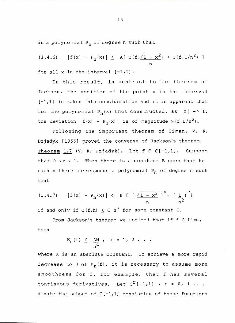
15

is a polynomial Pn of degree n such that

(1.4.6) lf( x ) - Pn(x) I .s_ A[ w(f, / 1 - x 2 ) + w (f,1/n 2 ) ]

n

for all x in the interval [-1,1].

In this result, in contrast to the theorem of

Jackson, the position of the point x in the interval

[-1,1] is taken into consideration and it is apparent that

for the polynomial Pn(x) thus constructed, as lxl -> 1,

the deviation lf(x) - Pn(x) I 2 is of magnitude w (f,1/n ).

Following the important theorem of Timan, V. K.

Dzjadyk [1956] proved the converse of Jackson's theorem.

Theorem 1.7 (V. K. Dzjadyk). Let f e C[-1,1]. Suppose

that O < a < 1. Then there is a constant B such that to

each n there corresponds a polynomial Pn of degree n such

that

(1.4. 7) lf(x) - Pn(x) I .s_ B- ( ( l l x 2 ) a +

n

a 1 ) } ~2

if and only if w (f,h) .s_ Cha for some constant C.

From Jackson's theorem we noticed that if f e Lipa ,

then

En(f) .s_ AM, n = 1, 2 ••• na

where A is an absolute constant. To achieve a more rapid

decrease to O of En(f), it is necessary to assume more

smoothness for f, for example, that f has several

continuous derivatives. Let cr[-1,1] , r = O, 1 .•.

denote the subset of C[-1,1] consisting of those functions

16

which possess r continuous derivatives on [-1,1]. For

this class of functions, Dunham Jackson proved also the

following direct theorem.

Theorem 1.8 (D. Jackson). If f e c(r) [-1,1], then

( 1. 4. 8) En ( f) ~ Ar ( 1 / n) r w ( f ( r) , 1 / n) , n = l, 2, • • •

For many important contributions we refer to the work

of G. G. Lorentz [1983].

Spline Approximation

One uses polynomials for approximation because they

can be evaluated, differentiated and integrated easily and

in finitely many steps using just the basic arithmetic

operations of addition, subtraction and multiplication.

But there are limitations of polynomial approximations.

For example, the polynomial interpolant is very sensitive

to the choice of interpolation points. If the function to

be approximated is badly behaved anywhere in the interval

of approximation, then the approximation is poor every­

where.

This global dependence on local properties can be

avoided when using piecewise polynomial approximation.

Concerning piecewise polynomial approximation, Professor

I. J. Schoenberg remarked that "polynomials are wonderful

even after they are cut into pieces, but the cutting must

be done with care. One way of doing the cutting leads to

the so-called spline functions" (Schoenberg [1946],

p. 46).

17

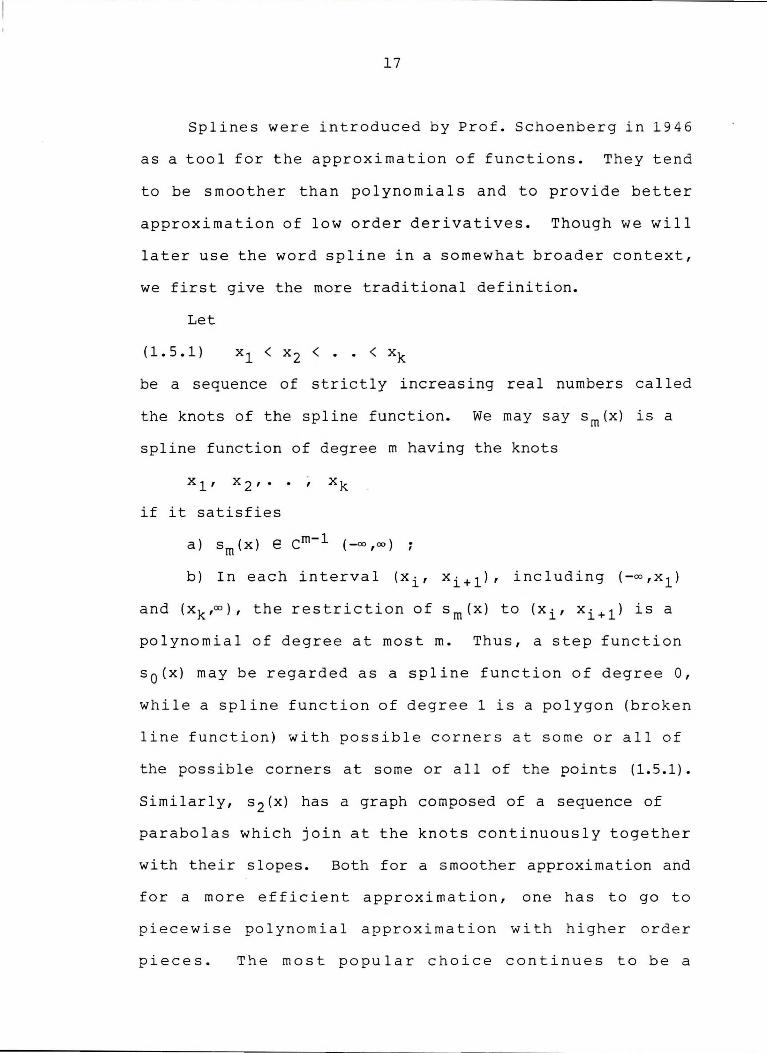
Splines were introduced by Prof. Schoenberg in 1946

as a tool for the approximation of functions. They tend

to be smoother than polynomials and to provide better

approximation of low order der i va ti ves. Though we wi 11

later use the word s p 1 ine in a somewhat broader con text,

we first give the more traditional definition.

Let

(1.5.1)

be a sequence of strictly increasing real numbers called

the knots of the spline function. We may say sm(x) is a

spline function of degree m having the knots

x 1 , x 2 , .. , xk

if it satisfies

a) s (x) e cm-l (-oo ,oo) ; m

b) In each interval (xi, xi+l), including (-00 ,x 1 )

and (xk,00), the restriction of sm (x) to (xi, xi+l) is a

polynomial of degree at most m. Thus, a step function

s 0 (x) may be regarded as a spline function of degree 0,

while a spline function of degree 1 is a polygon (broken

line function) with possible corners at some or all of

the possible corners at some or all of the points (1.5.1).

Similarly, s 2 (x) has a graph composed of a sequence of

parabolas which join at the knots continuously together

with their slopes. Both for a smoother approximation and

for a more efficient approximation, one has to go to

piecewise pol y nomial approximation with higher order

pieces. The most popular choice continues to be a

18

piecewise cubic approximating function. Various kinds of

cubic splines are in use in numerical analysis. The ones

most commonly used are complete cubic splines, periodic

cubic splines and natural cubic splines.

A spline function of degree m with k knots is repre­

sented by a different polynomial in each of the k+l

intervals into which the k knots divide the real line. As

each polynomial involves m + 1 parameters, the spline

function involves a total of (m+l) (k+l) parameters.

However, the continuity conditions stated ear 1 ier impose

certain constraints on those parameters. At each knot,

the two adjoining polynomial arcs must have equal

ordinates and equal derivatives of order 1, 2, ••• ,

m - 1. Thus, rn constraints are imposed. It is easy to

see that every spline function s(x) of degree rn with the

knots x 1 , x 2 , •• , xk has a unique representation in the

form

(1.5.1) k

s(x) = Pm(x) + L CJ· (x - XJ·)! j=l

where Prn(x) denotes a polynomial of degree m and

(1.5.2)

Also

(1.5.3)

x m = xrn +

= 0

X ) 0

X < 0

C · = (1/(rn) !) [ s(rn) (x •+) - s(rn) (x--) } • J J J

The class of "natural" spline functions was intro­

duced by Prof. Schoenberg [1946]. A spline function s(x)

19

of odd degree 2p-l with knots x 1 , x 2 , .. , xk is called

a natural spline function if the two polynomials by which

it is represented in the two end intervals (- ,x 1 ) and

(xk,+ ) are of degree p-1 or less. It is easy to express

the natural spline functions by

(1.5.4)

where

s(x)

k

k = Pp-1 (xl + I

j=l C- (X-X·) 2P-l

J J +

I cj xjr = O, r = p, p+l, •• , 2p-l. j=l

The following theorem states an important interpola­

tion property of natural spline functions.

Theorem 1.9 Let (xi, yi), i= 1, 2, •• , k, be given

data points, where the X · 1

S 1 form a strictly increasing

sequence, and let p be a positive integer not exceeding n.

Then there is a unique natural spline function s(x) of

degree 2p - 1 with the knots xi such that

(1.5.5) s(xi) = Yi , i = 1, 2, ... , k.

Natural spline functions possess certain impressive

optimal properties and can be shown to be the "best"

approximating functions in a certain sense. This is the

content of the next theorem.

Theorem 1.10 Let P(x) be the unique natural spline

function that interpolates the data points (xi,Yi),

i = 1, 2, .• , k, in accordance with Theorem 1. 7. Let

f(x) be any function of the class c(P) that satisfies the

conditions

20

(1.5.6) f(X·) =y., l l

i = 1, 2, •• , k.

Let (a,b) be a finite interval containing all the knots

xi. Then

(1.5. 7) b

f [ f ( p ) ( X ) ] 2 dx > b

f [ s ( p ) ( x ) ] 2 dx a a

with equality only if f(x) = s(x).

The effectiveness of the spline approximation can be

explained to a considerable extent by its striking conver-

gence properties. Interesting contributions were made by

J. N. Ahlberg and E. N. Nilson [1964], C. DeBoor and G.

Birkhoff [1964], A. Sharma and A. Meir [1967], M. J.

Marsden [1972], T. R. Lucas [1974], E. w. Cheney and F.

Schurer [1968], C. A. Hall [1968], C. A. Hall and w. w.

Meyer [1976], and A. K. E. Atkinson [1968]. As a good

reference on splines which offers a good comparison of the

approximating properties of polynomials and splines, we

recommend A Practical Guide to Splines by C. DeBoor

[1978].

First we discusss error analysis for the class of

functions f(x) e c( 2) with period one. Let

(1.5.8) = 1

be a division of [0,1] of mesh gauge

(1.5.9)

where

I 21

A periodic cubic spline function Yn (x) is . a function

composed of a cubic polynomial in each of the intervals of

(xiJt=o with the requirement that

Yn(x) e c( 2 ) (0,1]

and

i = o, 1, 2.

It was observed by Walsh, Ahlberg and Nilson [1962] that

there exists a unique periodic spline function Yn(x) which

interpolates f(x) at the points xn,l· It was shown that

Yn(x) and y'n(x) converge uniformly to f(x) and f'(x)

respectively as hn -> 0. Later Ahlberg and Nilson [1966]

studied the more delicate question of the convergence of

y"n(x) to f"(x). Writing

(1.5.10) ;\ . = n,1 hn, i + 1 / ( hn, i + hn, i + 1) '

i = 1, 2,

and

An= maxo~i~k l '- n,i - l/ 2 I ' where form= kn, " n,m+l is taken as

(hn,l + hn,m)/hn,l '

they show that

y'' (x) -> f''(x) n

uniformly provided that

hn -> 0 and An-> 0.

After this result, I. J. Schoenberg [1964a] raised the

question that it would be very interesting to find out to

what extent the condition An-> 0 is really necessary in

the above mentioned theorem. The above theorem together

22

with toe open problem of Schoenberg lead to important

contributions by Birkhoff and DeBoor [1964], and Meir and

Sharma [1969] which we turn to describe.

In 1964, Garrett Birkhoff and Carl DeBoor made the

following contribution. Let f(x) e C'[0,1] and let

(1.5.11) [X }k o = xo < x1 < i i=O'

be a partition. The function f(x) is now interpolated by

a cubic spline function s(x) (called a complete cubic

interpolation spline function) which means that s(x) is a

cubic polynomial when restricted to each interval

(xi,xi+l), and s (x) e c( 2 ) [0,1].

uniquely defined by the conditions

Moreover s (x) is

(1.5.13) f(xi) = s(xi)

f'(0) = s'(0),

f' (1) = s' (1)

i = 0, 1, •• , k

This first important result concerning the error analysis

yielded the following theorem.

Theorem 1.11 Let f(x) e c( 4) [0,1].

e(r) = f(r)_ s(r)

Denote

There are constants cr(m), r = 0, 1, 2, 3, depending

only on m > 0, such that

(1.5.13)

provided that

h . = l

m I

r = 0, 1, 2, 3,

23

h = max hi ,

and 11 I I denotes the supremum norm.

The authors go a step further and prove a convergence

theorem related to f e c( 3) [0,1].

Theorem 1.12 Let f"' (x) be absolutely continuous on

[0,1]. Let (xiJ1= 0 ,n (where k depends on n) be a sequence

of partitions of [0,1] such that hn = maxihi,n ->Oas

n -> Let mh,n <mas n -> Let en(x) be the error

incurred when f(x) is interpolated by a spline function on

Then

le'''nl -> 0

uniformly on (0,1] as n -> 00

The next important development came with some

interesting results by Prof. A. Sharma and A. Meir (1967]

concerning degree of approximation of spline interpola­

tion. This paper does away with some annoying assumptions

under which uniform convergence of the interpolating cubic

spline and its derivatives was proven earlier (see above

for these restrictions).

Theorem 1.13 Let f(x) be continuous and periodic with

period unity. Let

(1.5.15)

where

qn = max• • l.' J

Let sn(x) be the cubic spline of period unity with

joints (or knots) xn,i' i = O, 1, .. , n in [0,1], such

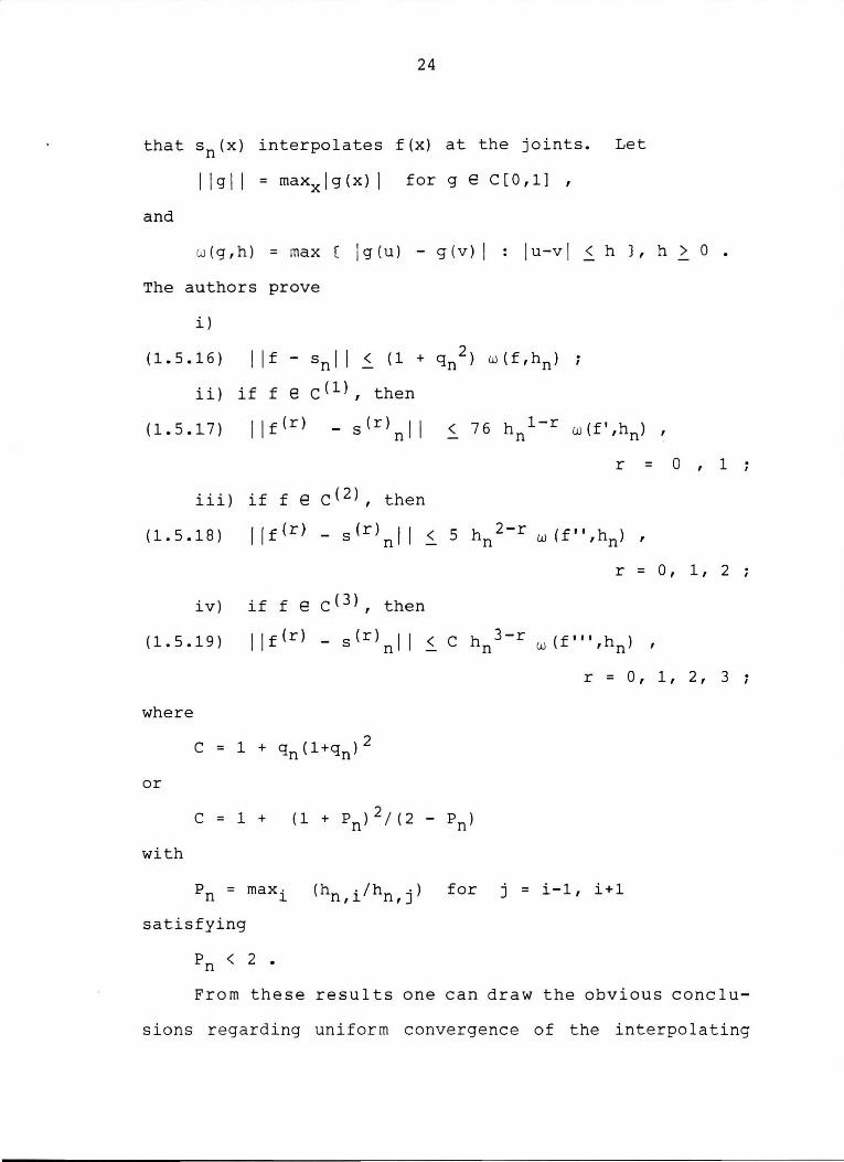
24

that sn(x) interpolates f(x) at the joints. Let

I lg! I = maxxlg(x) I forge C[0,1] ,

and

w ( g , h) = max ( I g ( u ) - g ( v ) I

The authors prove

!u-v ! < h }, h > 0 •

i)

( 1. 5 .16) I If - sn I I _s_ ( 1 + qn 2 ) w ( f, hn) ;

ii) if f e c(l), then

(1.5.17)

iii)

(1.5.18)

iv)

(1.5.19)

where

or

with

I If (r>

if f e

I It ( r >

if f e

I If (rl

P = max . n l

satisfying

- s(r)nl I

C ( 2) , then

- s(r)nll

C ( 3) , then

- s(r)nl I

< 76 hn 1-r w (f' ,hn)

r

< 5 hn 2-r w (f",hn) - ,

r =

< C hn 3-r (f"' h ) - w , n

r = 0,

for j = i-1, i+l

,

= 0 , 1

0 , 1, 2

,

1, 2, 3

From these results one can draw the obvious conclu­

sions regarding uniform convergence of the interpolating

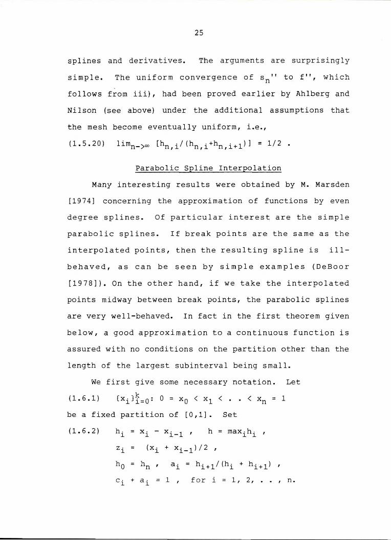
25

splines and derivatives. The arguments are surprisingly

simple. The uniform convergence Of S II n to f'', which

follows from iii), had been proved earlier by Ahlberg and

Nilson (see above) under the additional assumptions that

the mesh become eventually uniform, i.e.,

(1.5.20)

Parabolic Spline Interpolation

Many interesting results were obtained by M. Marsden

(1974] concerning the approximation of functions by even

degree splines. Of particular interest are the simple

parabolic splines. If break points are the same as the

interpolated points, then the resulting spline is ill­

behaved, as can be seen by simple examples (DeBoor

[1978]). On the other hand, if we take the interpolated

points midway between break points, the parabolic splines

are very well-behaved. In fact in the first theorem given

below, a good approximation to a continuous function is

assured with no conditions on the partition other than the

length of the largest subinterval being small.

We first give some necessary notation. Let

(1.6.1)

be a fixed partition of [0,1]. Set

(1.6.2) h- = X• - xi-1 ' h = max -h , l l l. l

z . = (X· + xi-1)/2 ' l l.

ho = hn , a- = hi+l/(hi + hi+l) ' l

C· + a - = 1 ' f o r i = 1, 2 , . . n.

l l

26

Let

ye C[0,1] , y(0) = y(l) ,

I I YI I = sup ( I Y (x) I : 0 < x < 1 }

such that y is extended periodically with period 1.

A function s(x) is defined to be a periodic quadratic

spline interpolant associated with y and (xi}r=O if

(1.6.3) a) s(x) is a quadratic expression on each

b) s(x) e C' [0,1] ,

c) s(O) = s(l) , s' (0) = s' (1)

d) s(zi) = y(zi) , i = 1, 2, . , n.

The following theorems were obtained by Marsden.

Theorem 1.14 (Marsden). Let (xiJ1=o be a partition of

[0,1], y(x) be a continuous 1- periodic function and s(x)

be the periodic quadratic spline interpolant associated

with y and (xi}~=O·

Then

(1.6.4)

(where

llsill < 2 IIYII, lleill < 2w(y,h/2),

I lei I ~ 3 w(y,h/2) •

11s11 < 2 IIYII,

S· = s(x-) and e- = y(x-) - s(x-) ). l l l l l

The constant 2 which appears in the first of the above

equations can not, in general, be decreased.

Theorem 1.15 (Marsden). Let y and y' be continuous 1-

periodic functions. Then

(1.6.5) ll s'ill ~ 2IIY'II,

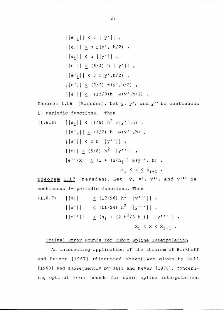
27

lle'ill .s. 3 IIY'II,

lleill < h w{y', h/2),

lleill < h IIY'II,

lie II< {5/4) h IIY'II,

I le'il I _s_ 3 w{y' ,h/2) ,

lle'II < {9/2) w{y',h/2),

I le 11 < {13/8)h w {y' ,h/2) •

Theorem 1.16 {Marsden). Let y, y', and y'' be continuous

1- periodic functions. Then

(1.6.6) I ieil I .S. (1/8) h 2 w {y' ',h) ,

I le'il I .S. {1/2) h w {y' ',h) ,

lle'II .S. 2 h IIY" l l,

!lei I .S. (5/8) h 2 I IY" II , le'' {x) I _s_ [1 + (h/hi)] w (y'', h) ,

xi .S. x .S. xi+l.

Theorem 1.17 (Marsden). Let y, y', y", and y"' be

continuous 1- periodic functions. Then

(1.6.7) I le I I < (17/96) h3 IIY"'ll ,

I I e' II < (11/24) h2 IIY"'II ,

lle"II < [h • + l

(2 h 2 /3 hi)] IIY'"II ,

Xi< X < Xi+l •

Optimal Error Bounds for Cubic Spline Interpolation

An interesting application of the theorem of Birkhoff

and Priver [1967] (discussed above) was given by Hall

[1968] and subsequently by Hall and Meyer [1976], concern­

ing optimal error bounds for cubic spline interpolation.

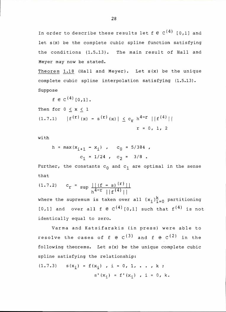
28

In order to describe these results let f e c( 4 ) [0,1] and

let s(x) be the complete cubic spline function satisfying

the conditions (1.5.13).

Meyer may now be stated.

The main result of Hall and

Theorem 1.18 (Hall and Meyer). Let s(x) be the unique

complete cubic spline interpolation satisfying (1.5.13).

Suppose

f e c( 4 l [0,11.

Then for O < x < 1

(1.7.1) Jf(r) (x) - s(r) (x) I < cr h 4-r I jf( 4 ) 11

r = 0, 1, 2

with

CO= 5/384 ,

c 1 = 1/24 , c 2 = 3/8 .

Further, the constants c 0 and c 1 are optimal in the sense

that

(1. 7 .2) cr = sup I I ( f - s l ( r) I I h 4-r JJf( 4 lJJ

where the supremum is taken over all (xi}1=o partitioning

[0,1] and over all f e c( 4 ) [0,1] such that f( 4 ) is not

identically equal to zero.

Varma and Katsifarakis (in press) were able to

resolve the cases of f e c( 3 ) and f e c( 2 ) in the

following theorems. Let s(x) be the unique complete cubic

spline satisfying the relationship:

(1.7.3)

s'(x•) = f'( x• ) l l

i = 0, k.

29

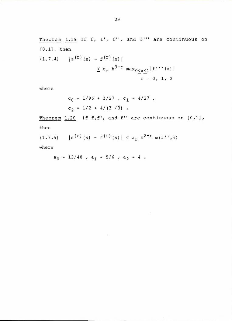
Theorem 1.19 If £, £', £", and £"' are continuous on

[ O, 1 l , then

(1.7.4) /s(r) (x) - f(r) (x) I

where

< cr h 3-r maxO<x<llf''' (x) I r = O, 1, 2

c 0 = 1/96 + 1/27 , c 1 = 4/27,

C2 = 1/2 + 4/(3 /3).

Theorem 1.20 If f,f', and f" are continuous on (0,1],

then

(1.7.5) [s(r} (x) - f(r} (x} I < ar h 2-r w(f' ',h)

where

a 0 = 13/48 , a 1 = 5/6 , a 2 = 4 •

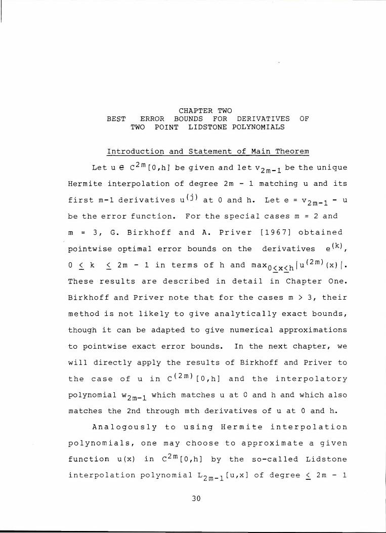
CHAPTER TWO BEST ERROR BOUNDS FOR DERIVATIVES OF

TWO POINT LIDSTONE POLYNOMIALS

Introduction and Statement of Main Theorem

Let u e c 2 m [0,h] be given and let v 2 m-l be the unique

Hermite interpolation of degree 2m - 1 matching u and its

first m-1 derivatives u(j) at 0 and h. Let e = v 2 m-l - u

be the error function. For the special cases m = 2 and

m = 3, G. Birkhoff and A. Priver [1967] obtained

pointwise optimal error bounds on the derivatives e(k),

0 < k < 2m - 1 in terms of h and maxO<x<h I u (2 m) (x) j.

These results are described in detail in Chapter One.

Birkhoff and Priver note that for the cases m > 3, their

method is not likely to give analytically exact bounds,

though it can be adapted to give numerical approximations

to pointwise exact error bounds. In the next chapter, we

will directly apply the results of Birkhoff and Priver to

the case of u in c( 2 m) [0,h] and the interpolatory

polynomial w2rn-l which matches u at 0 and hand which also

matches the 2nd through mth derivatives of u at 0 and h.

Analogously to using Hermite interpolation

polynomials, one may choose to approximate a given

function u(x) in c 2 m[0,h] by the so-called Lidstone

interpolation polynomial L 2 m_ 1 [u,x] of degree< 2m - 1

30

31

matching u and its first m - 1 derivatives u( 2 j) at 0 and

h. Thus L 2m_ 1 [u,x] satisfies the following conditions

(where we assume h = 1):

(2.1.1) L ( 2 P)[u 0] =u( 2 P)(O), 2m-1 '

L ( 2P) [u 1] = u ( 2P) (1) 2m-l '

p = o, 1, , m - 1.

The explicit formula for L2m_ 1 [u,x] is

(2.1.2)

where

(2.1.3)

and

(2.1.4)

m-1 I u (2i) (1)

i=0 L2m-l[u,x] = . ( X)

l

m-1 + L u(2i) (0) i(l-x)

i=0

2· ..L.=, B2i+l(l+x) (2i+l) ! 2

, for i > 1

Here Bn(x) denotes the Bernoulli polynomial

(2.1.5)

and where the constant B· is given by J

(2.1.6) B. = J

That (2.1.2) in fact satisfies (2.1.1) follows from

the facts

1d 2 Pl (0l = 0 p = 0, l

1, . . , i ;

(2.1.7) id 2P) (1) = 0 p = 0, 1 , . . , i - 1 ; l

APi) (1) = 1 l

The main object of this chapter is to obtain

pointwise optimal error bounds for

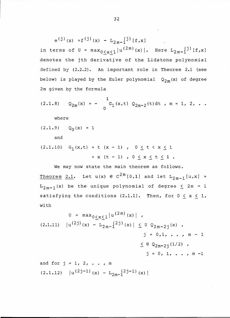
32

e(j) (x) =f (j) (x) - L 2 m-ij) [f,x]

in terms of U = maxO<x<llu( 2 m) (x) 1- Here L 2 m-ij) [f,x]

denotes the jth derivat~ve of the Lidstone polynomial

defined by (2.2.2). An important role in Theorem 2.1 (see

below) is played by the Euler polynomial o2 m(x) of degree

2m given by the formula

(2.1.8)

where

(2.1.9)

and

02m (x) =

o0 (xl = 1

1 G 1 ( x, t) Q 2 m- 2 ( t) d t , m = 1 , 2 , • .

0

(2.1.10) G1 (x,t) = t (x - 1) 0 ( t ( X ( 1

= X (t - 1) , 0 ( X ( t ( 1 .

We may now state the main theorem as follows.

Theorem 2.1. Let u(x) e c 2 m [0,1] and let L 2 m-l [u,xJ =

L 2 m_ 1 (x) be the unique polynomial of degree~ 2m - 1

satisfying the conditions (2.1.1). Then, for O < x < 1,

with

u = max O < x < 1 I u ( 2 m) ( x) I ,

(2.1.11) lu( 2 j) (x) - L 2 m_{ 2 j) (x) I < U 0 2 m-2j (x) ,

and for j = 1, 2, •. , m

j = 0,1, •• , m - 1

< u o2m_ 2 j (1/2) ,

j = O, 1, •• , m -1

(2.1.12) I u ( 2 j -1) ( x) - L 2 m-12 j -1) ( x) I

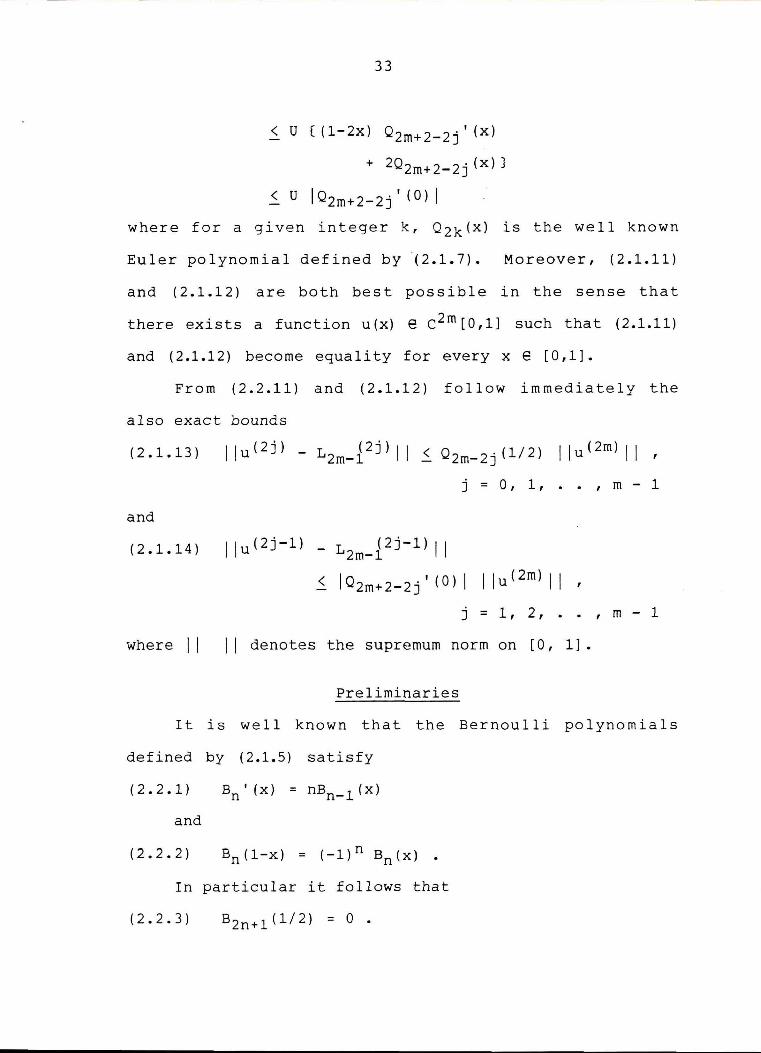
33

< u ( (l-2x) Q2m+2-2j' (x)

+ 2Q2m+2-2j(x)}

< u I02m+2-2j'(O)I

where for a given integer k , Q 2 k(x) is the well known

Euler polynomial defined by (2.1.7). Moreover, (2.1.11)

and (2.1.12) are both best possible in the sense that

there exists a function u(x) e c2m[0,1] such that (2.1.11)

and (2.1.12) become equality for every x e [0,1].

From (2.2.11) and (2.1.12) follow immediately the

also exact bounds

(2.1.13) I lu( 2 j) - L2m-i 2 j) 11 < 02m-2j( 1 / 2 ) I lu( 2m) 11 ,

j = 0, 1, .• , m - 1

and

(2.1.14) I I u ( 2 j- l) - L 2 m- i 2 j- l) I I

< I02m+2-2j' (0) I I lu ( 2m) 11 ,

j = 1, 2, . . ' m - 1

where I I 11 denotes the supremum norm on [ 0, 1] •

Preliminaries

It is well known that the Bernoulli polynomials

defined by (2.1.5) satisfy

(2.2.1)

and

(2.2.2) Bn (1-x) = (-1) n Bn (x) •

In particular it follows that

(2.2.3) B 2n+l (1/2) = 0 •

34

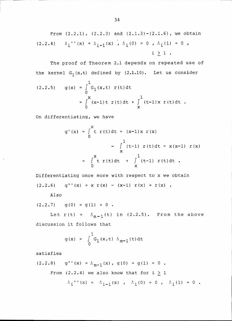
From ( 2. 2 .1) , ( 2. 2. 3) and ( 2 .1. 3) - ( 2 .1. 6) , we obtain

(2.2.4) J\i" (x) = J\i-1 (x) ' J\i (0) = O ' J\i (1) = 0 '

i > 1 .

The proof of Theorem 2.1 depends on repeated use of

the kernel G1 (x,t) defined by (2.1.10). Let us consider

1 (2.2.5) g(x) = f G1 (x,t) r(t)dt

0 X 1

= J (x-l)t r(t)dt + J (t-l)x r(t)dt . 0 X

On differentiating, we have

X g I (X) = J t r(t)dt + (x-l)x r(x)

0 1

J (t-1) r(t)dt - x(x-1) r(x) X

X 1 = f t r(t)dt + J (t-1) r(t)dt .

0 X

Differentiating once more with respect to x we obtain

(2.2.6) g' ' ( x) = x r ( x) - ( x-1) r ( x) = r ( x) .

Also

(2.2. 7) g(O) = g(l) = 0 .

Let r ( t) = J\m_ 1 (t) in (2.2.5). From the above

discussion it follows that

satisfies

(2.2.8)

1 g(x) = f G1 (x,t) J\m_ 1 (t)dt

0

g' ' ( x) = A m-l ( x) , g ( O) = g ( 1) = O

From (2.2.4) we also know that for i > 1

J\ i'' (x) = Ai-1 (x) , J\, (0) = 0, l

35

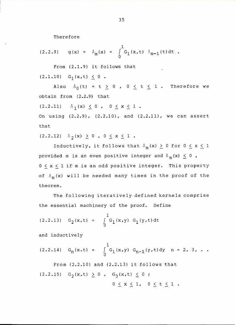
Therefore

1 (2.2.9) g ( x) = Am ( x) = f G1 (x,t) Am_ 1 (t)dt ..

0

From (2.1.9) it follows that

(2.1.10) G1 (x,t) < 0 •

Also A0 (t) = t > 0 , 0 < t < 1 •

obtain from (2.2.9) that

(2.2.11)

Therefore we

On using (2.2.9), (2.2.10), and (2.2.11), we can assert

that

(2.2.12) A2(X) ~ 0 , 0 < x < 1 .

Inductively, it follows that 11.rn(x) ~ 0 for O < x < 1

provided rn is an even positive integer and 11.m(x) i O ,

0 < x < 1 if mis an odd positive integer. This property

of 11.m(x) will be needed many times in the proof of the

theorem.

The following iteratively defined kernels comprise

the essential machinery of the proof. Define

(2.2.13) G2 (x,t) =

and inductively

(2.2.14) Gn(x.t) =

1 f G1(x,y) G1 (y,t)dt 0

1 f G1 (x,y) Gn_ 1 (y,t)dy n = 2, 3, •. 0

From (2.2.10) and (2.2.13) it follows that

(2.2.15) G2 (x,t) ~ 0, G3 (x,t) < 0

0 < X < 1, 0 < t < 1 .

36

In general

(2.2.16) (-l)nGn(x,t) > 0

0 ( X ( 1, 0 ( t ( 1 .

Finally, let us define

(2.2.17) h(x) = 1

f Gn(x,t) q(t)dt. 0

We note again that h(x) uniquely satisfies

h (2n) (x) = q (x)

h (2k) (0) = h (2k) (1) (2.2.18)

= 0 ' k = O, 1, . • I n-1 .

We also need some of the known properties of Euler

polynomials introduced in (2.1.7) and (2.1.8). We can

easily verify that

(2.1.19) 02~• (x) = Q2n-2(x)

o2n(O) = o2n(l) = O.

Furthermore,

02J2p) (0) = Q (2p) (1) 2n = 0 I p

(2.2.20) Q (2n) (l) 2n = Q (2n) (O)

2n = (-l)n

Q (2j) (x) 2n = (-1) j O2n-2j (x)

Using (2.2.13) we note that

1 f G1 (x,t) dt , 0

1 f G1 (x,t) Q 2 (t) dt 0

1 1

= 0 ' 1, . .

= f G1 (x,t) [ 0

f G1(t,y) dy] dt 0

, n-1,

37

and in general,

(2.2.21) Q2m(x) = (-l)m

Explicitly some of the first Euler polynomials are

given by

= x(l-x) 2 !

o4 (x) = x 2 ( 1-x) 2 +x ( 1-x) , 4 !

= x 3 (1-x) 3 +3x 2 (1-x) 2 +3x(l-x) 6 !

Proof of Theorem 2.1

Let P 2 rn-l denote the class of polynomials of degree

< 2m-1. Following the notation used by Birkhoff and

Priver [1967] we shall denote

(2.3.1) Gm ( i ' j ) ( X, t) = c) i + j Gm ( x, t)

Since L 2 m_ 1 [u,x] = u(x) for u(x) e P 2 m-l it follows

from the Peano theorem that for u e c2m[0,1]

(2.3.2) e(x) =: u(x) - L2m_ 1 [u,x]

1 = f Gm(x,t) u ( 2m) (t) dt

0

where Gm (x,t) is the Peano kernel defined by (2.1.10) and

(2.2.14). Differentiating (2.3.2) we have

(2.3.3) = u( 2 j) (x)- L ( 2 j) [u x] 2 m-1 '

1 . = f Gm( 2 J,O)(x,t) u( 2 m)(t) dt.

0

Let us substitute u (x) = Q 2 m (x) (as defined by

(2.1.7)) in (2.3.3) and use various properties as given by

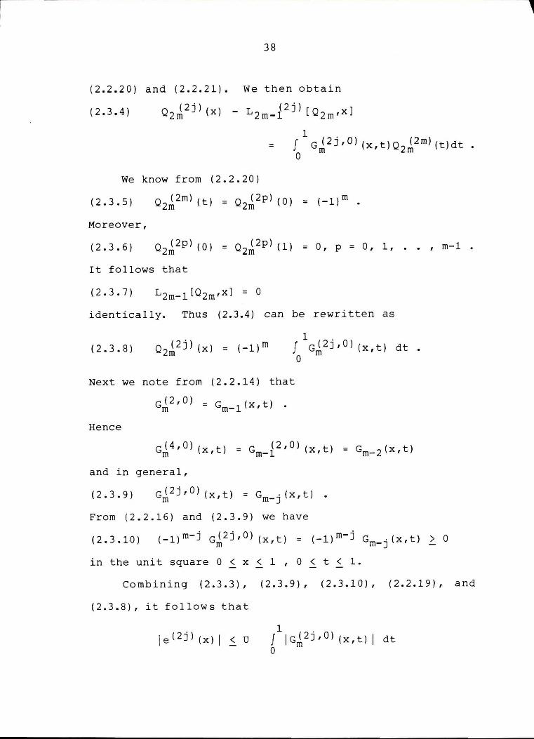
38

(2.2.20) and (2.2.21). We then obtain

(2.3.4) Q2~2j) (x) - L2m-i2j) [Q2m'x]

1 . = J GJ2J ,0) (x,t)02J2rn) (t)dt

0

We know from (2.2.20)

(2.3.5)

Moreover,

(2.3.6) Q2J 2Pl (0) = Q2J 2Pl (1) = 0, p = 0, 1, •• , m-1 •

It follows that

(2.3.7)

identically. Thus (2.3.4) can be rewritten as

(2.3.8) 1 .

f GJ 2 J 'O) ( x, t) d t . 0

Next we note from (2.2.14) that

G( 2 ,0) = G (x t) m m-1 ' •

Hence

GJ 4 ' O ) ( X , t)

and in general,

= G ( 2 ,0) (X t) = m-1 '

(2.3.9) GJ2 j ,O) (x,t) = Gm-j (x,t) •

From (2.2.16) and (2.3.9) we have

Gm_ 2 (x, t)

(2.3.10) ( -1) m-j GJ 2 j 'O) ( x, t) = (-1) m- j Gm-j ( x, t) > 0

in the unit square O ~ x ~ 1 , 0 < t < 1.

Combining (2.3.3), (2.3.9), (2.3.10), (2.2.19), and

(2.3.8), it follows that

je( 2 j) {x) I ~ U 1 .

J JGJ2J,O) (x,t) I dt 0

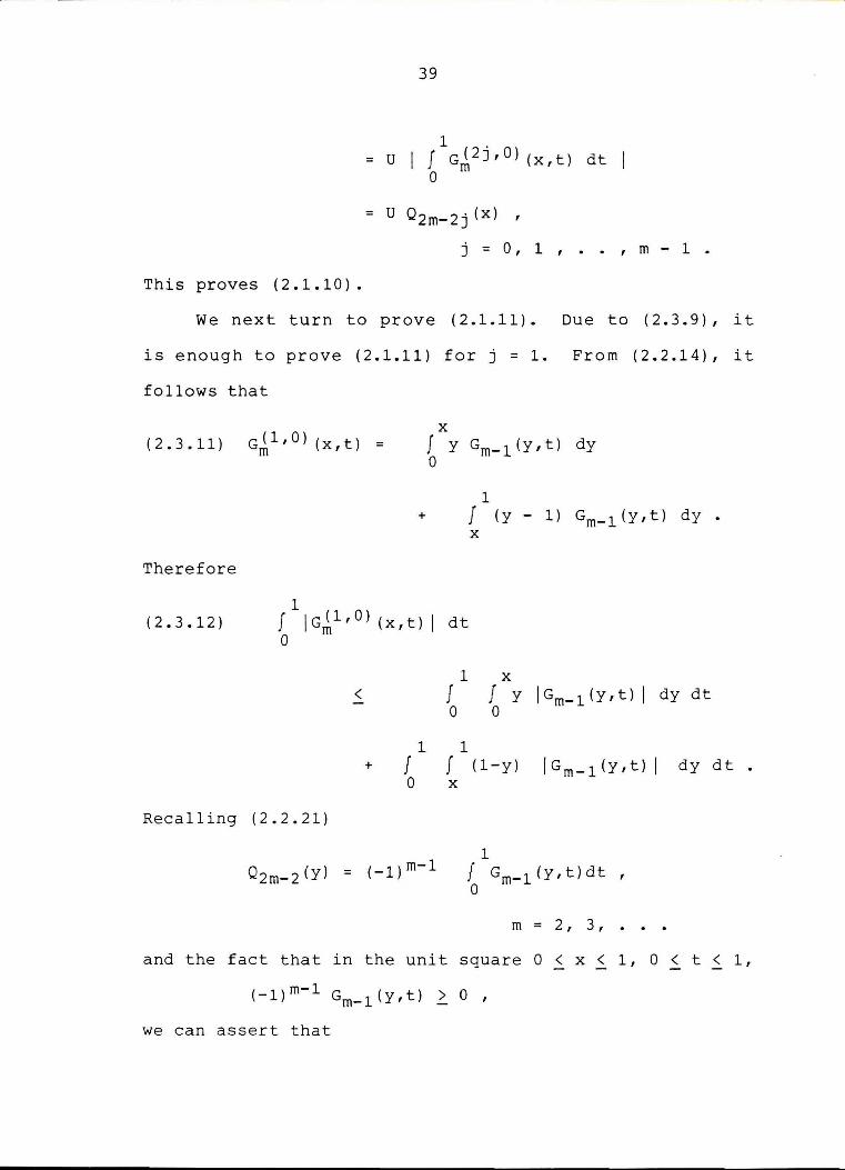
This proves (2.1.10).

39

1 . = U f GJ 2 J,O) (x,t) dt I

0

= U Q2m-2j (x) '

j = 0, 1 , •. , m - 1 .

We next turn to prove (2.1.11). Due to (2.3.9), it

is enough to prove (2.1.11) for j = 1. From (2.2.14), it

follows that

( 2 • 3 • 11) GJ l ' O) ( x, t) =

Therefore

X

f y Gm-l (y,t) dy 0

1 + f (y - 1) Gm-l (y,t) d y •

X

(2.3.12) 1

J IGJl,O) (x,t) I dt 0

<

Rec a 11 ing ( 2. 2. 21)

1 X

f f Y IGm-l (y,t) I dy dt 0 0

1 1 + f f (1-y) JGm_ 1 (y,t) I dy dt.

0 X

1 f Gm- l ( y, t) d t , 0

m = 2, 3,

and the fact that in the unit square O < x < 1, 0 < t < 1,

(-l)m-1 Gm-l(y,t) > 0 '

we can assert that

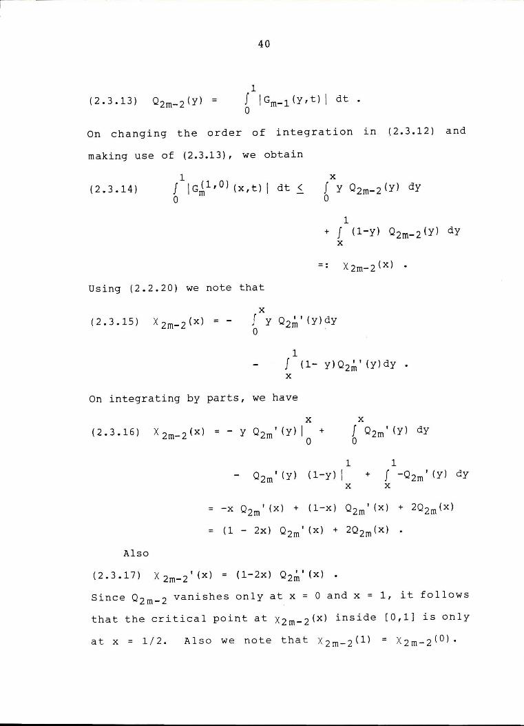
(2.3.13) 0 2m_ 2 (y) =

40

1 f I Gm- l ( y, t) I d t • 0

On changing the order of integration in (2.3.12) and

making use of (2.3.13), we obtain

(2.3.14) 1

f I GJ l ' O ) ( x , t) I d t < 0

X

f Y 02rn-2(Y) dy 0

1 + f (l-y) 02m-2(Y) dy

X

Using (2.2.20) we note that

( 2 • 3 • 15) X 2 m- 2 ( x) =

X

f y 02~• (y)dy 0

1 f (1- y)Q 2~• (y)dy X

On integrating by parts, we have

X X

(2.3.16) X 2m-2 (x) = - Y 02rn' ( Yl I + 0

f 02m' (y) dy 0

1 1 02rn'(yl (l-yll + f -Q2m' (y) dy

X X

= -x 02rn' (x) + (1-x) 02m' (x) + 2Q 2m(x)

= ( 1 - 2x) Q2m' (x) + 2Q 2m(x)

Also

(2.3.17) X 2m-2' (x) = (1-2x) Q I I (X) 2m .

Since Q2 m- 2 vanishes only at x = 0 and X = 1, it follows

that the critical point at x2 m_ 2 (x) inside [0,1] is only

at x = 1 / 2. Also we note that x 2 m_ 2 (1) = X2m-2 (0) •

41

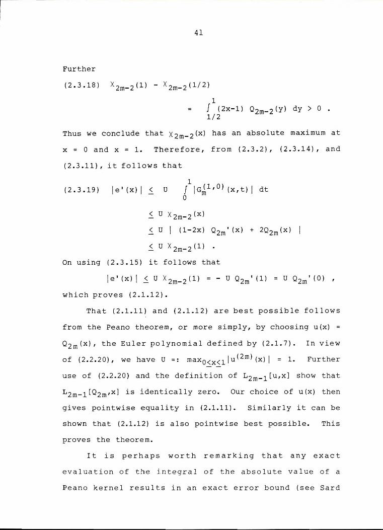
Further

(2.3.18) x2m_ 2 (1) - X2m_ 2 (1/2)

1 = f (2x-1) o2m_ 2 (y) dy > 0

1/2

Thus we conclude that x2m_ 2 (x) has an absolute maximum at

x = O and x = 1. Therefore, from (2.3.2), (2.3.14), and

(2.3.11), it follows that

(2.3.19) I e' (x) I < U 1

J IGJl,O) (x,t) I dt 0

< U X 2m-2 (x)

< U (1-2x) Q2m' (x) + 2Q 2m(x)

< U X 2m-2 ( 1) .

On using (2.3.15) it follows that

I e ' ( x) I ~ U X 2 m- 2 ( 1 ) = - U Q 2 m ' ( 1 ) = U Q 2 m ' ( 0 ) '

which proves (2.1.12).

That (2.1.11) and (2.1.12) are best possible follows

from the Peano theorem, or more simply, by choosing u(x) =

0 2 m (x), the Euler polynomial defined by (2.1. 7). In view

of (2.2.20), we have U =: maxo<x<llu( 2m)(x)I = 1. Further

use of (2.2.20) and the definition of L2m_ 1 [u,x] show that

L2m_ 1 [Q 2m,x] is identically zero. Our choice of u(x) then

gives pointwise equality in (2.1.11). Similarly it can be

shown that (2.1.12) is also pointwise best possible. This

proves the theorem.

It is perhaps worth remarking that any exact

evaluation of the integral of the absolute value of a

Peano kernel results in an exact error bound (see Sard

42

[1963] or Stroud [1974]). Generally error bounds

resulting from integration of a Peano kernel under the

assumption that u{x) e ck[a,b] also hold for u having

piecewise continuous kth derivative on [a,b], and even for

u having (k-l)st derivative absolutely continuous on

[a,b]. In the case given here we can thus expand the

class of functions for which the error bounds of Theorem

2.1 hold and hence are best possible.

As Theorem 2.1 is stated for function u{x) 2m times

continuously differentiable, it al so holds when the 2mth

derivative is merely piecewise continuous on [0,1].

Moreover the theorem holds even for the case that u(x) has

its {2m-1) st derivative absolutely continuous. In this

last case U, instead of being the max of the 2mth deriva­

tive on [0,1], beaomes the "L infinity" norm of the gener­

alized 2mth derivative. In the following chapters the

classes of functions k times continuously differentiable,

the class of functions having piecewise continuous kth

derivative and the class having k-lst derivative absolute­

ly continuous may be treated as being interchangeable.

CHAPTER THREE MORE POLYNOMIAL ERROR BOUNDS

Introduction and Statement of Theorems

Let u e c( 2 m+ 2 ) [0,h] be given. It follows from a

result of Schoenberg [1966] that there exists a unique

polynomial w2m+l [u,x] of degree < 2m+l satisfying

(3.1.1) w2m+l[u,0] = u(0) ,

W2m+l (p) [u,0] = u (p) (0)

w2m+l (p) [u,h] = u(p) [u,h]

w2m+l[u,h] = u(h)

p = 2, 3, • , m + 1 .

Theorems 3.1 and 3.2 will give bounds on U ( j) ( X)

w(j) 2 m+l(x) for the cases m = 2 and m = 3 of polynomials

w 2 rn+l satisfying (3.1.1).

The polynomial w 2 m+l[u,x] can be expressed in

relation to the Hermite polynomial v 2 m-l [u" ,x]. To

illustrate the relation between w2 rn+l and v 2 m-l' let h = 1

and let v 2 m_ 1 [g,x] be the Hermite polynomial of degree at

most 2m - 1 matching g =: u" and its first m - 1

derivatives at 0 and 1. We can represent v 2 rn_ 1 [g,x] as

(3.1.2) v2m-1 [g,x] = A0 (x)g(0) + B0 (x)g(l)

+ Al (x)g' (0) + Bl (x)g' (1)

+ A2(x)g" (0) + B 2 (x)g" (1)

+ Am-1 ( x) g ( m-1) ( 0) + Bm-1 ( x) g ( m-1) ( 1)

43

44

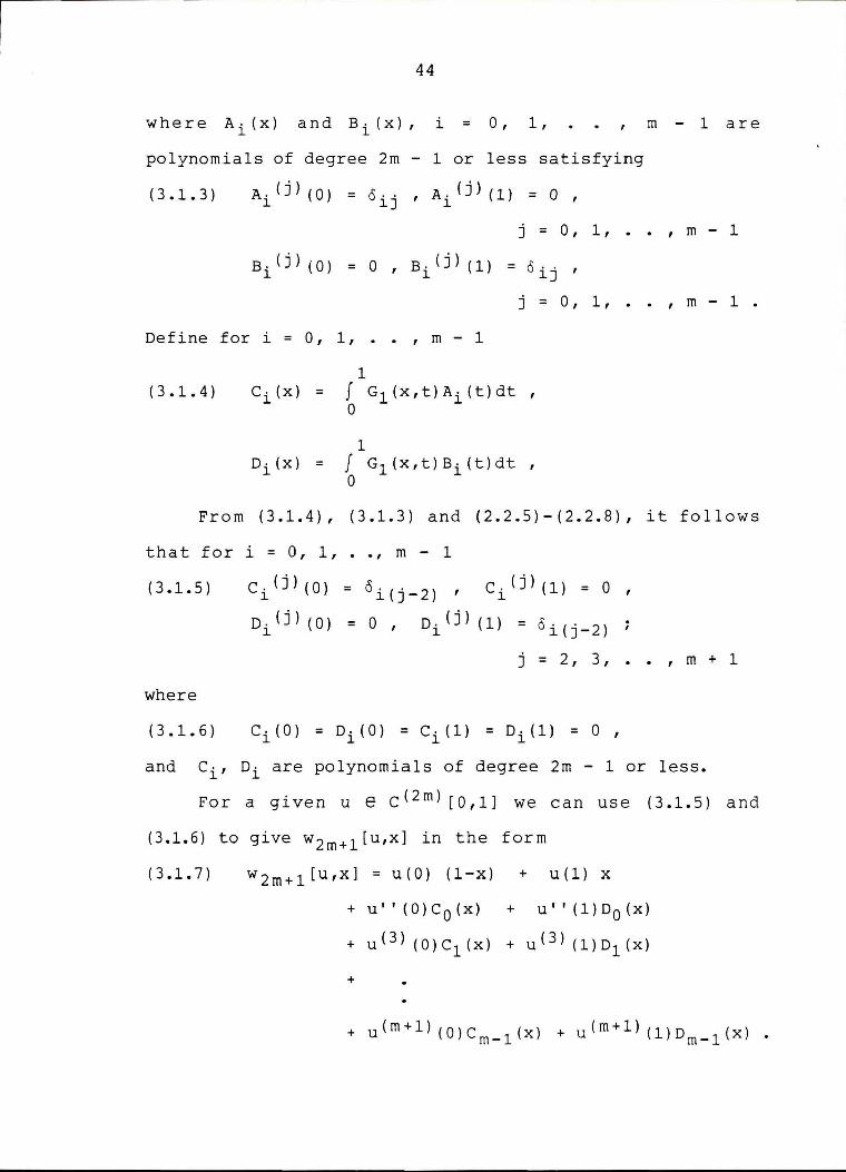
where Ai (x) and Bi (x), i = 0, 1 , . . , m - 1 are

polynomials of degree 2m - 1 or less satisfying

(3.1.3) A-(j)(O) = O··, A.(j)(l) = 0, l l] l

j = 0, 1, •• , m - 1

Bi (j) (0) = 0 , Bi (j) (1) = 0 ij ,

j = 0, 1, •. , m - 1.

Define for i = O, 1, •• , m - 1

(3.1.4) C · (x) = l

D · (x) = l

1 f G1 (x,t)Ai(t)dt, 0

1 f G1(X,t)Bi(t)dt, 0

From (3.1.4), (3.1.3) and (2.2.5)-(2.2.8), it follows

that for i = 0, 1, . . , m - 1

(3.1.5) c.(j)(O) = l

( . ) oi(j-2) , Ci J (1) = 0 ,

D · ( j) ( 0) l = 0 , Di (j) (1) = oi(j-2)

j = 2, 3, .. , m + 1

where

(3.1.6)

and Ci, Di are polynomials of degree 2m - 1 or less.

For a given u e c( 2 m) [0,1] we can use (3.1.5) and

(3.1.6) to give w2 m+l [u,x] in the form

(3.1.7) w 2 m+l[u,x] = u(O) (1-x) + u(l) x

+ u" (0)C 0 (x) + u" (l)0 0 (x)

+ u( 3 ) (O)C1(X) + u( 3 ) (l)D1(X)

+

45

Form= 2 and m = 3, we give (3.1.7) explicitly. For

m = 2, if u e C ( 6 ) [0,1], -then the unique quintic w5 [u,x]

matching u and its second and third derivatives at O and 1

is given by

(3.1.8) w5

(u,x] = (1-x) u(O) + x u(l)

+ u"(O)

+ u''(l)

[-7x/20 + x 2 /2 - x 4 /4 + x 5 /10]

[-3x/20 + x 4 /4 - x 5 /10]

+ u' '' (0) [-x/20 + x 3 /6 - x 4 /6 + x 5 /20]

+ u''' (1) [x/30 - x 4 ;12 + x 5 /20]

For u e c( 8 ) [0,1], the unique polynomial w7 [u,x] of

degree~ 7, matching u and its second, third and fourth

derivatives at O and 1 is given by

(3.1.9) w7

[u,x] = (1-x) u(O) + x u(l)

+ u"(O)

+ U I I ( 1)

[-Sx/14 + x 2 /2 - x 5;2 + x 6 /2 - x 7 /7]

[-x/7 + x 5 ;2 - x 6 /2 + x 7 /7]

+ u( 3 )(0) [-13x/210 + x 3 /6 - 3x5 /10

+ 4x 6 /15 -x 7 /14]

+ u( 3 ) (1) [4x/105 - x 5 /s + 7x 6 /30 - x 7 /14]

+ u( 4 ) (0) [-x/210 + x 4 /24 - 3x 5 /40

+ x 6 ;20 - x 7 /84]

+ u( 4 ) (1) [-x/280 + x 5 /40 - x 6 /30 + x 7 /84] •

The following theorem concerns the quintic

interpolant w5 .

Theorem 3.1 Let u e c6 [0,1] and let w5 [u,x] satisfy

(3.1.10) w5

(p) [u,O] = u (p) (0) ,

w5

(P) [u,1] = u(p) (1) , p = O, 2, 3 •

46

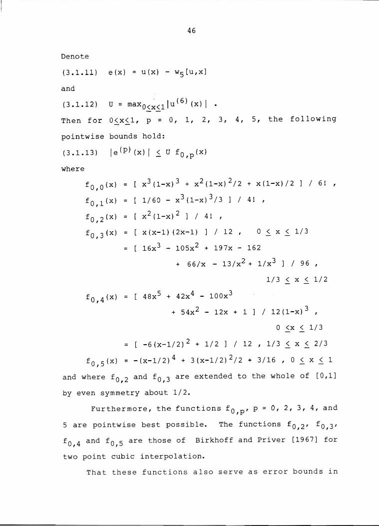
Denote

(3.1.11) e(x) = u(x) - w5 [u,x]

and

(3.1.12) . ( 6)

U = maxO<x<l I u (x) I • Then for o.s_x.s_l, p = O, 1, 2, 3, 4, 5, the following

pointwise bounds hold:

(3.1.13)

where

fo,o<xl = x 3 (1-x) 3 + x 2 (1-x) 2 /2 + x(l-x)/2 ] I 6 !

fQ,l(X) = 1/60 - x 3 (1-x) 3 /3 ] I 4 ! '

fo,2(X) = x 2 (1-x) 2 ] I 4 ! ' fo,3(X) = x(x-1) (2x-1) I 12 0 < X < 1/3

= 16x3 - 105x2 + 197x - 162

+ 66/x - 13/x2 + 1/x3 ] I 96 ' 1/3 ( X < 1/2

fo,4(X) = [ 48x5 + 42x4 - 100x3

+ 54x 2 - 12x + 1] / 12(1-x) 3 ,

= [ -6 ( x-1 / 2) 2 + 1 / 2 ] / 12

0 .s_x .s_ 1/3

1/3 .s_ X .s_ 2/3

'

f 0 , 5 (x) = -(x-1/2) 4 + 3(x-1/2) 2 /2 + 3/16 , o < x < 1

and where £0 , 2 and £0 , 3 are extended to the whole of [0,1]

by even symmetry about 1/2.

Furthermore, the functions fo,p' p = 0, 2, 3, 4, and

5 are pointwise best possible. The functions f 0 , 2 , f 0 , 3 ,

f 0 , 4 and fo,s are those of Birkhoff and Priver [1967] for

two point cubic interpolation.

That these functions also serve as error bounds in

47

the present case is a consequence of the fact that

w 511 [u,x] · is the unique cubic matching u" and u"' at 0

and 1. In other words w 511 [u,x] is the Hermite cubic

interpolation v 3 [g,x] where g = u". The error bounds

given by Birkhoff and Priver in terms of maxO<x<llg( 4 ) (x) I

are now expressed in terms of U = maxo<x< 1 1 u ( 6 ) (x) I (as

g( 4 ) is in fact u ( 6 )).

Denoting

(3.1.14) C = p p = 0, 1, .• , 5

we have

CO = 11 1 cl = 1 1 , c2 = 1

~ -

24 6 ! 2 6 ! 4 !

C3 = 1/3 , C4 = 1 , C5 = 1 . 9 4! ff 2

From (3.1.14) and (3.1.13) it follows that for every

u e c( 6 ) [O,lJ

(3.1.15) maxO<x<lle(P) (x) I < cp U

Remark 3.1 Note that

p = o, 1, .. , 5 .

p = 0, 1, .• , 5 •

If we set u(x) = t 0 , 0 (x) then we have

e (X) = f 0 , 0 (xl - w 7 [f 0 , 0 ,xJ

= fo,o(X) and U = maxo~x~1lfo,0( 6 ) I = 1

By Remark 3.1 we see that for u(x) = f 0 , 0 (x) equality is

attained in (3.1.15) for p = 0, 1, 2, 3, 4, 5. The

constants cp are thus the smallest possible.

The next . theorem gives error bounds for w7 , analogous

to the error bounds for w5 given in Theorem 3.1.

48

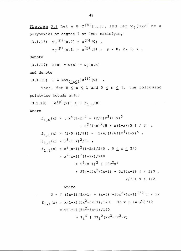
!h~£!~~ 3.2 Let u e c(B) [0,1], and let w 7 [u,x] be a

polynomial of degree 7 or less satisfying

(3.1.16) w7

<P) [u,O] = u(p) tO) ,

w7

(P) [u,1] = u(p) (1) , p = O, 2, 3, 4 •

Denote

(3.1.17) e(x) = u(x) - w7 [u,x]

and denote

( 3 . 1. 18 ) U = max O < x < 1 I u ( 8 ) ( x) I • Then, for O ~ x ~ 1 and O < p < 7, the following

pointwise bounds hold:

(3.1.19) Je(P) (x) I ~ U f 1 ,p(x)

where

f 1 , 0 (x) = [ x 4 (1-x) 4 + (2/5)x3 (1-x) 3

+ x 2 (1-x) 2 /5 + x(l-x)/5] / 8! ,

t1

,1

(x) = (1/5) (1/8!) - (1/4) (1/6 ! )x4 (1-x) 4 ,

t 1 , 2 (x) = x 3 (1-x) 3 /6!

t 1 , 3 (x) = x 2 (x-1) 2 (1-2x)/240 , 0 < x < 2/5

= x 2 (x-1) 2 (1-2x)/240

where

+ T 4 (x-1) 2 [ 10T2x 2

+ 2T(-1Sx 2+2x+l) + 5x(5x-2) ] I 120 ,

2/5 ( X ( 1/2

T = (3x-1) (Sx+l) + (x-1) (-15x2 +6x+l) l/ 2 ] / 12

f 1 , 4 ( X ) = X ( 1-X ) ( 5 X 2 - 5 X + 1 ) / 12 0 , 0 ( X ( ( 4-/6) / 1 0

= x(l-x) (Sx2-sx+l) /120

+ T14 [ 2T 1

2 (2x 3-3x 2+x)

49

where

+ 12T1 (-5x3 +sx2-3x)/5

+ (10x 3-isx 2 +9x-l) ] / 12 ,

for (4-/6)/10 < x < (3-/3)/6

T1

= 15x 2 - 9x - (x-1) (3x(4-5x)) l/ 2] /6x(2x-1) ,

t 1 , 4 (x) = x(x-1) (Sx 2-sx+l)/120

+ w4x [ 1ow2 (2x 2-3x+l)

+ 4W(1Sx2-2lx+6)

+ 5(10x 2-12x+3)

+ 5(10x 2-12x+3) ]/60,

for (3-/3) /6 < x < (6-/6) /10

and where

W = [ 3(1-x) (Sx-2) + x(3(1-x) (Sx-1) ) 1 / 2 ] , 6 (x-1) (2x-l)

t 1 , 4 (x) = x(x-1) (Sx2-sx+l)/120

(6-/6) /10 i X < 1/2

t 1 , 5 (x) = (2x-1)(10x 2-1ox+l)/l20

where

+ w14 [ 2ow1

2 (6x 2-6x+l)

+ 24W1 (15x2-14x+2)

+ 30(10x2-8x+l) ] / 120 ,

0 ( X < (4-/6)/10

w1

= [ - 15x2 + 14x - 2 - x(3x(4-5x)) 1 / 2

12x2 - 12x + 2

= (2x-1) (10x 2-1ox+l) /120 ,

(4-/6)/10 < X < (6-/6)/10

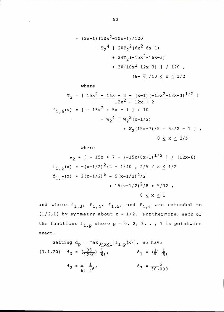
50

= (2x-1) (10x2-1ox+l) /120

where

- T24 20T 2

2 (6x 2-6x+l)

+ 24T 2 (-15x 2+16x-3)

+ 30(10x2-12x+3) ] / 120,

(6- 6)/10 < X ( 1/2

15x2 - 16x + 3 - (x-1) (-15x2 +18x-3) 1 / 2

12x2 - 12x + 2

f 1 , 6 (x) = [ - 15x2 + 5x - 1 ] / 10

where

- w 4 2 w2

2 (x-1/2)

+ w2 (15x-7) /5 + 5x/2 - 1 ] ,

0 ( X ( 2/5

w2 = [ - 15x + 7 - (-15x+6x+l) l/ 2 ] / (12x-6)

f 116 (x) = -(x-1/2) 2 /2 + 1/40 , 2/5 < x < 1/2

f 1 , 7 (x) = 2(x-1/2) 6 - 5(x-1/2) 4;2

+ lS(x-1/2) 2 /8 + 5/32 ,

0 ( X ( 1

and where f 1 , 3 , f 1 , 4 , f 1 , 5 , and f 1 , 6 are extended to

[1/2,1) by symmetry about x = 1/2. Furthermore, each of

the functions fl,p where p = 0, 2, 3, . , 7 is pointwise

exact.

Setting dp = max 0~x~1 Jf 1 ,p(x) I, we have

( 3 1 20 ) d = ( 93 ) 1 d (1) 1 • . 0 1280 8!' 1 = 5 8!

5 30,000

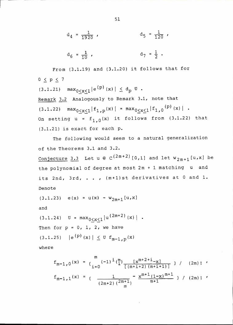
51

d - 1 7 - 2

From (3.1.19) and (3.1.20) it follows that for

0 < p .s_ 7

(3.1.21) maxo.s_x.s_lle(p) (x) I .s_ dp U •

Remark 3.2 Analogously to Remark 3.1, note that

(3.1.22) maxo.s_x.s_lif 1 ,P(x) I = maxo.s_x.s_ilf 1 , 0 (P) (x) I • On setting u = f 110 (x) it follows from (3.1.22) that

(3.1.21) is exact for each p.

The following would seem to a natural generalization

of the Theorems 3.1 and 3.2.

Conjecture 3.3 Let u e c( 2 m+ 2 ) [0,1] and let w2 m+l[u,x] be

the polynomial of degree at most 2m + 1 matching u and

its 2nd, 3rd,

Denote

• • I (m+l)st derivatives at O and 1.

(3.1.23) e(x) = u(x) - w2m+l[u,x]

and

(3.1.24) U - max I u ( 2 m + 2 ) ( x) I - 0<x<l •

Then for p = 0, 1, 2, we have

(3.1.25)

where

m fm-1,o(x) = (-l)i(f!l) [xm+2+i_x] } / ( l. -=----=:..:..:....---,-__;:,:....,...._..,... ( 2 m) ! '

i=0 [ (m+i+2) (m+i+l)]

fm-1,1 (X) = ( 1 - xm+l(l-x)m+l } / (2m) ! , ( 2m+ 2 ) (2m+l) m+l

m

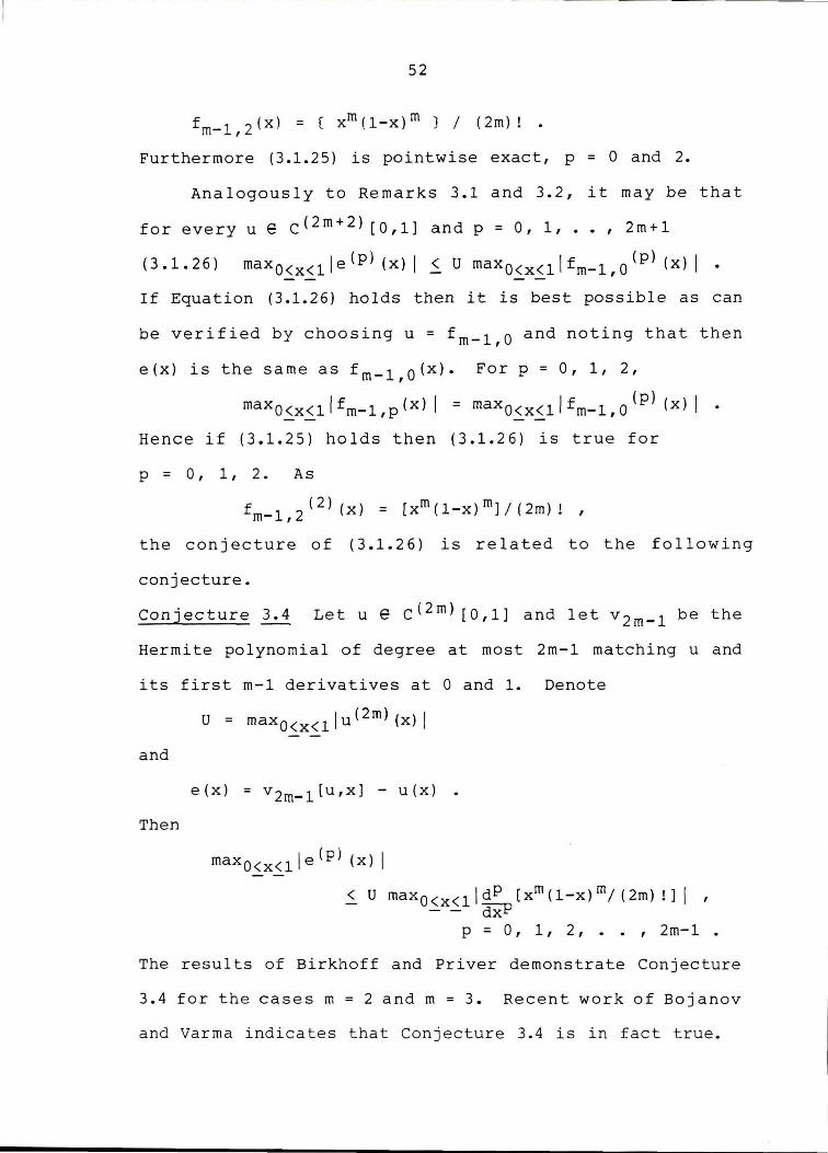
52

frn-l, 2 (x) = ( xrn(l-x)rn } / (2m) ! .

Furthermore (3.1.25) is pointwise exact, p = 0 and 2.

Analogously to Remarks 3.1 and 3.2, it may be that

for every u e c( 2 m+ 2 ) [0,1] and p = 0, 1, . . ' 2m+l

(3.1.26) maxO<x<lle(P) (x) I .s_ U maxo.s_x.s_llfm-l,O(p) (x) I • If Equation (3.1.26) holds then it is best possible as can

be verified by choosing u = frn-l,O and noting that then

e(x) is the same as fm-l,O(x). For p = O, 1, 2,

maxo.s_x.s_1lfm-l,p(x) I = rnaxo.s_x.s_1lfm-l,O (p) (x) I Hence if (3.1.25) holds then (3.1.26) is true for

p = 0, 1, 2. As

f ( 2 l(x) = [xm(l-x)m]/(2m)!, m-1,2

the conjecture of (3.1.26) is related to the following

conjecture.

Conjecture 3.4 Let u e c( 2 m) [0,1] and let v 2 m-l be the

Hermite polynomial of degree at most 2m-l matching u and

its first m-1 derivatives at O and 1. Denote

U = maxO<x<llu(2m)(x)J

and

e(x) = v 2m_ 1 [u,x] - u(x)

Then

maxO<x<l I e (p) (x) I

< u maxo<x<lldp [xm(l-x)m/(2m)!]I, - - dxP

p = O, 1, 2, •. , 2m-1 .

The results of Birkhoff and Priver demonstrate Conjecture

3.4 for the cases m = 2 and m = 3. Recent work of Bojanov

and Varma indicates that Conjecture 3.4 is in fact true.

53

The next theorem will concern an interpolatory

polynomial which enjoys a similar property to that of

the above conjectures. Let u e c( 4 ) [0,1]. Define

k 3 [u ,x] by

(3.1.27) k 3 [u,x] = u(O) (1-x) {1-2x) 2 + u{l/2) 4x(l-x)

+ u(l) x(l-2x) 2 + u' (1/2) 2x(l-x) (2x-1) •

Then k 3 [u,x] is the unique polynomial of degree 3 or less

satisfying

(3.1.28) k 3 [u,x] = u(O) , k 3 [u,1] = u(l) ,

k 3 [u,1/2] = u(l/2) k 3 ' [u,1/2] = u' (1/2)

Theorem 3.3. Let u € c( 4 ) (0,1]. Denote

e(x) = k 3 [u,x] - u(x) ,

U = maxO<x<lju(4)(x)I.

Then for p = 0, 1, 2, 3, we have

(3.1.29)

where

ie(p) (x) I < a U - p

ao = 1 / ( 2 8 4 ! ) ,

a 2 = (5/2) (1/4!)

a 1 = 1 / (2 2 4!) ,

a 3 = 1/2

That the ap are the best possible can be verified by

choosing

u(x) = [ x(l-x) (1-2x) 2 ] I (2 2 4!) •

Due to the similarity between the proof of Theorem

3.3 and several other proofs in the following chapters, it

would be redundant to prove it here.

54

Proof of Theorem 3.1

Let u e c( 6 ) [0,1]. Then

(3.2.1) w5 [u,x] = (1-x) u (0) + X u(l)

+ u"(0) [-7x/20 + x 2 /2 - x 4 /4 +

+ u"(l) [-3x/20 + x 4 /4 - x 5 ;10J

+ u"'(O) [-x/20 + x 3 /6 - x 4 /6 +

+ u"'(l) [x/30 - x 4 /12 + x 5 /20]

is the only polynomial of degree~ 5 satisfying

(3.2.2)

Define

(3.2.3)

Then

(3.2.4)

and

(3.2.5)

w5

(Pl[u,O] = u(P)(O)

w5

(P) [u,1] = u(P) (1)

e(x) = u(x) - w 5 [u,x] •

p = o, 2, 3 •

e(p) (0) = 0, e<P) (1) = 0, p = 0, 2, 3,

e ( 6 ) (x) = Q(x) =: u ( 6 ) (x) •

x 5 /10]

x 5 120J

In other words, e(x) is the unique solution of the

differential equation (3.2.5) with boundary conditions

(3.2.4). We can rephrase (3.2.4) and (3.2.5) as

(3.2.6)

and

(3.2.7)

d 2e = y(x) ,

dx 2

e(0) = 0, e(l) = 0 ,

~ = Q(x) '

dx 4

y(0) = y(l) = y'(0) = y'(l) = 0.

From (3.2.6) and (3.2.2)-(3.2.6), it follows that

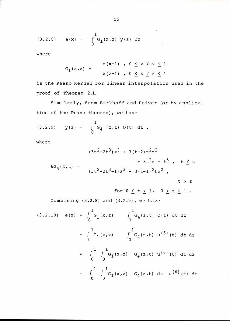
(3.2.8) e (X) =

where

55

1 f G1 (x,z) y(z) dz 0

G1 (x,z) = Z ( x-1) , 0 ( Z ( X ( 1

X ( z-1) , 0 ( X ( Z ( 1

is the Peano kernel for linear interpolation used in the

proof of Theorem 2.1.

Similarly, from Birkhoff and Priver (or by applica­

tion of the Peano theorem), we have

(3.2.9) y ( z) =

where

6G 4 ( z, t) =

1 f G4 (z,t) Q(t) dt , 0

(3t 2-2t 3 )z 3 + 3(t-2)t2 z 2

+ 3t2 z - t 3 , t < z

(3t 2-2t3-l)z 3 + 3(t-1) 2tz 2 ,

t > z

for O ~ t ~ 1, 0 < z < 1 .

Combining (3.2.8) and (3.2.9), we have

1 1 (3.2.10) e (x) = f G1 (x,z) f G4 (z,t) Q(t) dt dz

0 0

1 1 = f G1 (x,z) f G4 (z,t) u( 6 ) (t) dt dz

0 0

1 1 = f J G1 (x,z) G4 (z,t) u ( 6 ) (t) dt dz

0 0

1 1 = J f G1 (x,z) G4 (z,t) dz u( 6 ) (t) dt

0 0

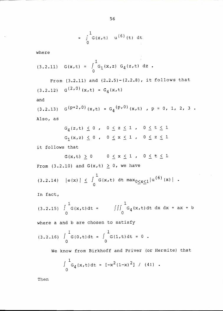
56

1 = f G(x,t) u ( 6 ) (t) dt

0

where

1 (3.2.11) G(x,t) = f G1(X,Z) G4(z,t) dz.

0

From (3.2.11) and (2.2.5)-(2.2.8), it follows that

(3.2.12) G( 2 ,0) (x,t) = G4 (x,t)

and

(3.2.13) G(p+ 2 ,0) (x,t) = G4

(p,O) (x,t) , p = 0, 1, 2, 3.

Also, as

G4 (z,t)

G1 (x,z)

it follows that

< 0

< 0

,

,

0 < z < 1 , 0 < t < 1

0 ( X ( 1 , 0 ( Z ( 1

G(x,t) > 0 0 < X < 1 , 0 < t < L

From (3.2.10) and G(x,t) ~ 0, we have

(3.2.14) le(x) I~ f 1G(x,t) dt maxo<x<llu( 6 ) (x) I .

0

In fact,

1 (3.2.15) f G(x,t)dt =

0

1 f Jf G4 (x,t)dt dx dx +ax+ b

0

where a and bare chosen to satisfy

1 1 (3.2.16) f G(O,t)dt = f G(l,t)dt = 0 •

0 0

We know from Birkhoff and Priver (or Hermite) that

1 f G4 (x,t)dt = [-x2 (1-x) 2 ] / (4!).

0

Then

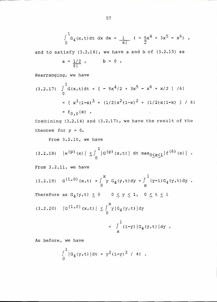
57

1 f G 4 ( x, t) d t dx d:X = 1 0 ~

( - sx4 + 3x 5 - x 6 ) , 2

and to satisfy (3.2.16), we have a and b of (3.2.15) as

a= 1/2 , 6!

Rearranging, we have

1 (3.2.17) f G(x,t)dt =

0

b = 0 •

- sx 4 ;2 + 3x5 - x 6 + x/2 ] /6!

= [ x 3 (1-x) 3 + (1/2)x2 (1-x) 2 + (1/2)x(l-x) ] / 6!

= fo,o(x) •

Combining (3.2.14) and (3.2.17), we have the result of the

theorem for p = 0.

From 3.2.10, we have

1 (3.2.18) le(P) (x) I ~J IG(p) (x,t) I dt maxO<x<llf( 6 ) (x) I •

0

From 3.2.11, we have

X 1 (3.2.19) G(l,O) (x,t) = f y G4 (y,t)dy + f (y-l)G4 (y,t)dy.

0 X

Therefore as G4 (y,t) ~ 0 0 ~ y ~ 1, 0 < t < 1

X

(3.2.20) !G(l,O) (x,t) I ~ f YIG 4 (y,t) !dy 0

1 + f ( 1-y) I G 4 ( y, t) I dy •

X

As before, we have

1 f IG4 (y,t) !dt = y 2 (1-y) 2 / 4! • 0

58

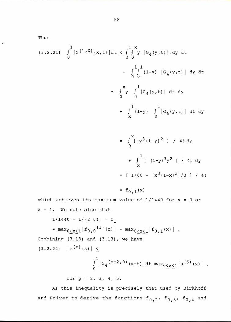
Thus

1 1 X

(3.2.21) J jG(l,O) (x,t) [dt < f f y jG4 (y,t) I . dy dt 0 0 0

1 1 + f f (1-y) IG4 (y,t) j dy dt

0 X

X 1 = f Y f IG4(y,t) I dt dy

0 0

1 1 + f (1-y)

X f IG4(y,t) I dt dy 0

X y3(1-y)2 = f [ ] I 4!dy

0

1 ( 1-y) 3y2 + f [ ] / 4 ! dy

X

= 1/60 - (x 3 (1-x) 3 )/3 ] I

= fo,l(X)

which achieves its maximum value of 1/1440 for x = 0 or

x = 1. We note also that

1/ 1440 = 1/ ( 2 6 ! ) = c1

= maxo~x~1lfo,o(l) (x) I = maxo~x~1lfo,1(x) I ·

Combining (3.18) and (3.13), we have

(3.2.22) je(P) (x) I ~

1

4 !

J jG 4 (p- 2 ,0) (x-t) jdt max 0<x<llu( 6 ) (x) I , 0

for p = 2, 3, 4, 5.

As this inequality is precisely that used by Birkhoff

and Priver to derive the functions f 0 , 2 , f 0 , 3 , f 0 , 4 and

59

f 0 , 5 , the theorem follows for p = 2, 3, 4, 5. The proof

of Theorem 3.2 is very similar and hence omitted.

CHAPTER FOUR A QUARTIC SPLINE

Introduction and Statement of Theorems

Among the many beautiful properties of the complete

cubic spline is the fact that for a given partition and

function values, the cubic spline is obtained by solving a

tridiagonally dominant system of equations.

Unfortunately, when one uses higher order complete splines

the bandwidth grows. In fact, for a 2m times continuous

spline of order 2m+l, the bandwidth of the system of

equations is 2m+l. Furthermore the diagonal becomes less

dominant ask increases.

It is na tura 1 then, to increase the order of the

spline but preserve bandwidth. Ideally we would hope to

increase the diagonal dominance and order of convergence.

In this chapter we introduce a quartic c( 2 ) spline which

gives O(h 5 ) rate approximation to a c(S) function. The

quartics are obtained by the solution of a tridiagonally

dominant system. As desired, it is more diagonally

dominant than the system associated with the complete

cubic spline.

The main result of this chapter will be to give an

exact error bound for the quartic spline discussed here.

We first give the definition.

60

61

Let f be a real-valued function defined on [a,b].

k Choose a partition (xi}i=O such that

a= x 0 < x 1 < ••• < xk = b •

Let zi = (xi-l + xi)/2, be the midpoint of [xi-l' xi] for

i = 1, 2, • , k and for these i set h · 1 = x · - x · 1 • ].- l. ].-

Definition 4.1 Given the function f and the partition

k (xi)i=O' we define a quartic spline s(x) such that

(4.1.1) s(x) e c2 [a,bl r, P 4 [xi-l' xi] , i = 1, 2, • , k;

x . ] denotes the functions which are l.

quartics when restricted to [xi-l' xi])

(4.1.2)

and

s(xi) = f(xi) for i = 0, 1, .• , k

s(zi) = f(zi) for i = 1, 2, •. , k

( 4 .1. 3) s ' (a) = f' (a) and s ' ( b) = f ' ( b) •

Lemma 4.1 Let f be a real-valued funtion defined on

[a, bl k and let (xi)i=O be a partition of [a,b]. A

quartic splines satisfies Equations (4.1.1) and (4.1.2)

if and only if s satisfies the tridiagonal system of

equations for i = 1, 2, •. , k - 1

(4.1.4)

-hi s' (xi_ 1 ) + 4(hi + hi_ 1 ) s' (xi) - hi-l s' (xi+ll

= -11 [(hi-1/hi) - (hi/hi_1 )] f(xi)

+ 16 [(hi-1/hi) f(zi+ll - (hi/hi-l) f(zi)]

- 5 [(hi-1/hi) f(xi+ll - (hi/hi-l) f(xi-l)]

where hi= xi+l - xi.

We will give the proof later.

62

Assuming from (4.1.2) that f(xi), i = 0, 1, •• , k

and f(zi), i = 1, 2, •• , k are known, then (4.1.4) is a

system of k - 1 equations in the unknown variables

s'(xi), i = 1, 2, .• , k. If we impose the conditions of

(4.1.3) that s' (x 0 ) = f' (a) and s' (xk) = f' (b) are given,

we have k-1 unknowns and the k - 1 diagonally dominant

equations (4.1.4). Lemma 4.1 thus assures us that s'(xi)

can be uniquely determined for given conditions (4.1.1)­

(4.1.3). As will be shown in the proof of the lemma, there

is, on any given subinterval [xi, xi+ll, a unique quartic

si(x) satisfying the five conditions

(4.1.5) S·(X·) = f(Xl.· ) l. l. si(zi+l) = f(zi+ll

s I • ( X. ) ::: s I ( Xl.· ) l. l.

s'i(xi+ll == s'(xi+l) .

Equations (4.1.4) are derived by imposing the conditions

that

For i == 1, 2, • • , k, si(x) is thus the restriction of

the spline s to [xi' xi+l].

Summarizing, unique solution of (4.1.4) implies that

s(x) is uniquely defined on each partition subinterval

[xi, xi+ll, i = 0, 1, •. , k-1, which is to say, on all

of [a, b]. We have shown

Corollary 4.1 The quartic spline of Definition 4.1 is, for

a given partition (xi}1=o and function f, unique.

We now make the comparisons with the complete cubic

spline more explicit. The system of equations

63

corresponding to (4.1.4) for the complete cubic spline has

left-hand side

his' (xi-1) + 2 (hi + hi-1) s' (xi) + hi-1 s' (xi+ll .

In comparison (4.1.4) is twice as diagonally dominant.

To interpolate the 2k + 1 function values f(xi) and

f (zi) using our c( 2 ) quartic required solving the

tridiagonal system of k - 1 equations (4.1.4). As the

cubic spline must match derivative and second derivative

values at each interior function value, interpolation of

the same 2k + 1 function values by the c( 2 l cubic spline

would entail solution of a system of 2k - 1 equations. In

other words, the matrix equation to be solved for the

quartic is only half as large as that required for the

cubic.

We can now state the main theorem of this chapter.

Given a partition (xi}t=o of [a, b], denote

h = maxO<i<k-lhi = maxO<i<k-l(xi+l-xi) •

For each x in [a,b], there exists i such that

0 < i < k - 1 and xi < X s_xi+l" We set t = (X - - Xi)/hi.

Theorem 4.1 Let f e c(S) [a,b] and let k (xi}i=O be a

partition of [a,b]. Let s (x) be the twice continuously

differentiable spline corresponding to f and

wheres satisfies (4.1.1)-(4.1.3). Then

(4.1.6) jf(x) - s(x) I ~ jc(t) I h 5 maxa<x<blf (S) (x) I / 5!

where

c(t) = [3t 2 (1-2t) (1-t) 2 + t(l-2t) (1-t)] / 6 •

Define

64

= ( / 1 - _J:. ) ( l / 5 + 2/30 ) / 6 . 4 m

It follows that

(4.1. 7)

Furthermore, neither lc(t) I nor c0

can be improved, as we

can show by letting f = x 5 /5! and letting k become

arbitrarily large for an equally spaced partition. An

approximate decimal expression for c0

is .0244482 and

c0

/5! is approximately .000203818 •

We will also show

(4.1.8) lf'(xi) - s'(xi)l

< h 4 maxa<x<blf (5 ) (x) I / 6!

and that this estimate is exact.

Related to Theorem 4.1 is the following conjecture.

Conjecture 4.1 Let f e c( 5 ) [a,b] and let (xi}1=o be a

partition of [a,b]. Let s(x) be the twice continuously

differentiable spline corresponding to f and

wheres satisfies (4.1.1)-(4.1.3). Then

(4.1.9) If' (x) - s' (x) I ~ h 4maxa<x<blf( 5 ) (x) I / 6! .

If Conjecture 4.1 holds, then the constant 1/6! can not be

improved. This conjecture has been verified numerically.

Remark 4.1 Given f e c 5 [a,b] and a partition (xiJf=o of

[a,b], let s be the quartic C ( 2 ) spline satisfying

(4.1.1)-(4.1.3). Then the supremum norm I lf(i) - s(i) 11

is of order hS-i maxa<x<b If (5 ) (x) I, i = o, 1, 2.

65

Theorem 4.1 demonstrates that the quartic c( 2) spline

gives the best possible order of approximation to

functions from the smooth class c( 5 l. We next discuss

interpolation to the much less smooth class of functions

which are merely continuous on [a,b]. As f' (a) and f' (b)

are not necessarily defined, we consider the quartic c< 2)

spline satisfying (4.1.1) and (4.1.2) with boundary

conditions

(4.1.10) s' (a) = s' (b) = 0 •

Denote w(f,h) =: sup!x-y!ih!f(x) - f(y) I. Theorem 4.2 Let f e C[a,b]. If (xiJf=o is the partition

of equally spaced knots, then for xi< x < zi+l = (xi+

, k - 1, we

have

(4.1.11) If (x) - s (x) I i c (t) w (f ,h) 0 < t < 1/2

and for zi+l ix i xi+l' or 1/2 ~ti 1

(4.1.12) lf(x) - s(x)! < c(l-t) w(f,h)

where c(t) = (1 + (13/3)t - 3t 2 - (58/3)t 3 + 16t 4 }

Note that maxO<t<l/ 2c(t) is approximately equal to

1.6572.

The bound of the preceding theorem is only valid for

equally spaced knots. For arbitrary partitions we can not

give a bound of this same form. However, if

we have the following theorem.

66

Theorem 4.1.3 Let f(x) e C[a,b], and lets be the c( 2 l

quartic spline satisfying (4.1.1), (4.1.2), and (4.1.9).

Then for xi~ x ~ zi+l' and i = 0, 1, 2,

(i.e., for 0 ~ t ~ 1/2 with t = (x - xi)/hi)

(4.1.13) Jf(x) - s(x) I < c 1 (t) w(f,h) ,

and for zi+l ~ x ~ xi+l' i.e. 1/2 ~ t ~ 1,

(4.1.14) Jf(x) - s(x) I _s. c 1 (1-t) w(f,h)

where

c 1 (t) = [1 + 10t2 - 28t3 + 16t4 ]

. . ' k - 1,

+ (8/3) [m 2 + m] [t(l-2t) (1-t)] •

Theorems 4.2 and 4.3 indicate that for suitable

partitions the quartic c 2 spline can provide acceptable

approximations to functions which are merely continuous on

[a,b].

Proof of Lemma 4.1

We first give an expression for the unique quartic

matching function and derivative values at endpoints and

function values at the midpoint. Specifically, let f be a

real-valued function defined on [0,1], and differentiable

at 0 and 1. Let

(4.2.1)

P1 (x) = 1 - llx2 + 18x3 - 8x 4 = (l-2x) (l-x) 2 (1+4x) ,

P2 (x) = 16x2 - 32x3 + 16x4 = 16x2 (1-x) 2 ,

P3 (x) = -sx2 + 14x3 - 8x 4 = -(1-2x)x2 [1+4(1-x)]

P4 (x) = x- 4x 2 + sx 3 - 2x 4 = x(l-2x)(l-x) 2

P5 (x) = x 2 - 3x3 + 2x 4 = x 2 (1-2x) (1-x) .

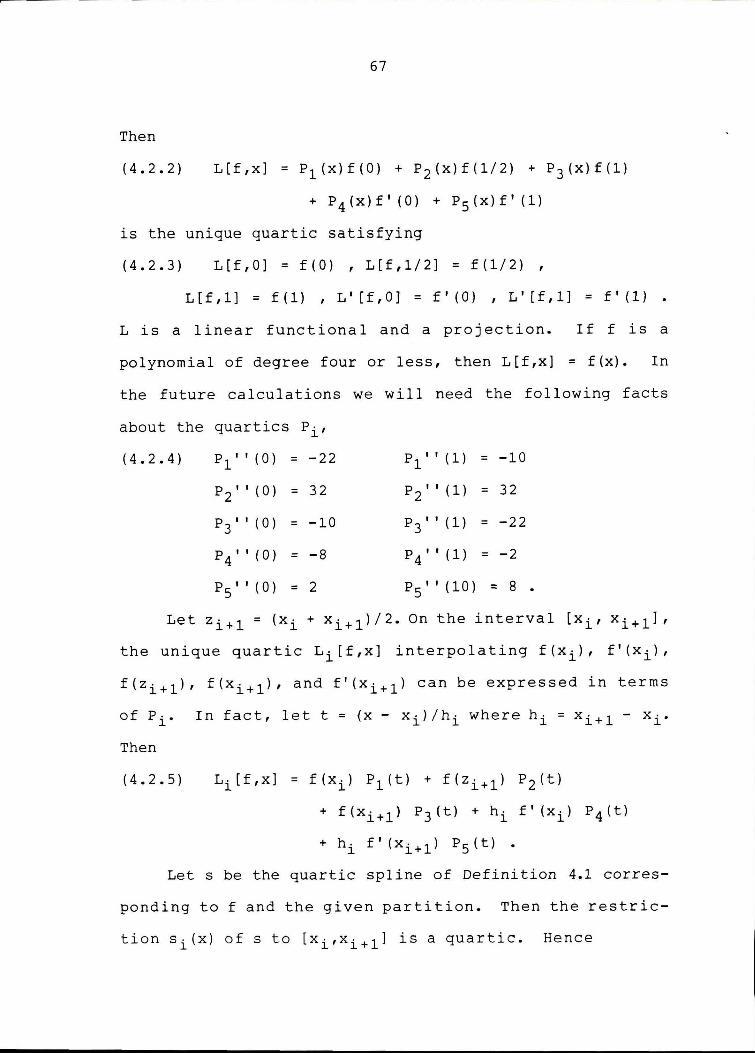
Then

(4.2.2)

67

L[f,x] = P1 (x)f(0) + P2 (x)f(l/2) + P3 (x)f(l)

+ P4 (x)f' (0) + P5 (x)f' (1)

is the unique quartic satisfying

(4.2.3) L[f,0] = f(0) , L[f,1/2] = f(l/2) ,

L[f,1] = f(l) , L' [f,0] = f' (0) , L' [f,1] = f' (1)

Lis a linear functional and a projection. If f is a

polynomial of degree four or less, then L[f,x] = f(x). In

the future calculations we will need the following facts

about the quartics p . , l

(4.2.4) P111 (0) = -22 P1

11 (l) = -10

P2 "(0) = 32 P211 (l) = 32

P311 (0) = -10 P3

11 (l) = -22

P 411 (0) = -8 P 4

11 (l) = -2

Ps"(0) = 2 Ps''(l0) = 8

Let z i + 1 = (X· l + xi+ll /2. On the interval [xi, xi+ll,

the unique quartic Li[f,x] interpolating f(xi), f'(xi),

f(zi+ll, f(xi+ll, and f'(xi+ll can be expressed in terms

of Pi. In fact, let t = (x - xi)/hi where hi= xi+l - xi.

Then

(4.2.5) Li[f,x] = f(xi) P1 (t) + f(zi+l) P2 (t)

+ f(xi+l) P3 (t) + hi f'(xi) P4 (t)

+ hi f I (Xi+l) P5 (t) .

Lets be the quartic spline of Definition 4.1 corres­

ponding to f and the given partition. Then the restric­

tion si(x) of s to [xi,xi+l] is a quartic. Hence

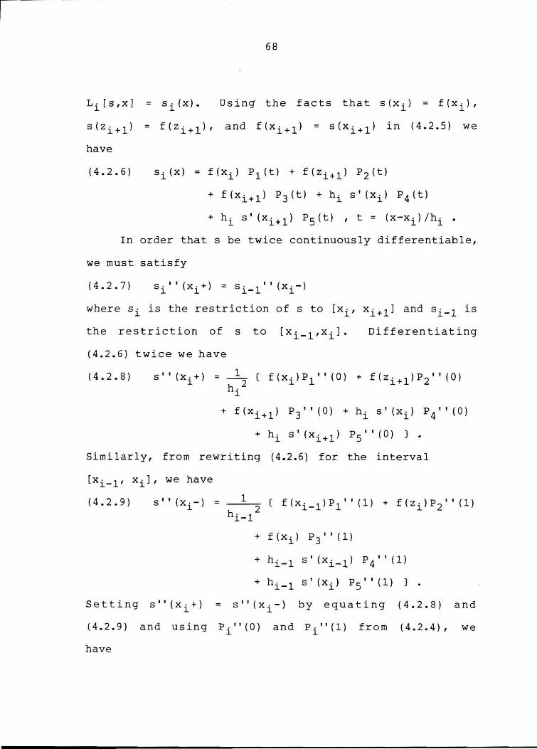
Li[s,x]

have

(4.2.6)

68

Using the facts that s(xi)

si(x) = f(xi) P 1 (t) + f(zi+l) P2 (t)

= f(X·), l

+ f(xi+l) P 3 (t) + hi s'(xi) P4 (t)

+ hi s' (xi+ll P 5 (t) , t = (x-xi) /hi •

In order thats be twice continuously differentiable,

we must satisfy

(4.2.7)

where si is the restriction of s to [xi, xi+l] and si-l is

the restriction of s to [xi_ 1 ,xi].

(4.2.6) twice we have

Differentiating

(4.2.8) s'' (xi+) = h~2 ( f(xi)P1'' (0) + f(zi+l)P2'' (0)

l

+ f(xi+ll P 311 (0) +his' (xi) P 4

11 (0)

+hi s'(xi+ll P5 "(0)}.

Similarly, from rewriting (4.2.6) for the interval

[x- 1 , x-], we have 1- 1

(4.2.9) s" (x - -) = 1

+ f(xi) P 311 (1)

+ hi-1 s' (xi-1) P4" (1)

+hi-l s'(xi) Ps"(l)}.

Setting s" (xi+) = s" (xi-) by equating (4.2.8) and

(4.2.9)

have

and using P-"(0) 1

and P - "(1) 1

from (4.2.4), we

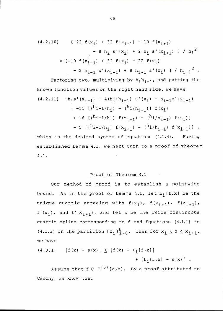
(4.2.10)

69

(-22 f(xi) + 32 f(zi+l) - 10 f(xi+l)

- 8 hi s'(xi) + 2 hi s'(xi+ll

= (-10 f(x. 1 ) + 32 f(z.) - 22 f(x-) 1- l l

} / h,2 l

- 2 hi-1 s' (xi-1) + 8 hi-1 s' (xi) } / hi-12 •

Factoring two, multiplying by hihi-l' and putting the

known function values on the right hand side, we have

(4.2.11) -his' (xi-l) + 4(hi+hi-l) s' (xi) - hi_ 1s' (xi+l)

= -11 [(hi-1/hi) - (hi/hi_1 )] f(xi)

+ 16 [ (hi-1/hi) f (zi+ll - (hi/hi-l) f (zi)]

- 5 [(hi-1/hi) f(xi+ll - (hi/hi-l) f(xi_ 1 )]

which is the desired system of equations (4.1.4). Having

established Lemma 4.1, we next turn to a proof of Theorem

4 .1.

Proof of Theorem 4.1

Our method of proof is to establish a pointwise

bound. As in the proof of Lemma 4.1, let Li[f,x] be the

unique quartic agreeing with f(xi), f(xi+ll, f(zi+l),

f'(xi), and f'(xi+ll, and lets be the twice continuous

quartic spline corresponding to f and Equations (4.1.1) to

(4.1.3) on the partition (xi}~=O· Then for xi~ x ~ xi+l'

we have

(4.3.1) if(x) - s(x) I < if(x) - Li[f,x] I

+ !Li[f,x] - s(x) I . Assume that f e c(S) [a,b]. By a proof attributed to

Cauchy, we know that

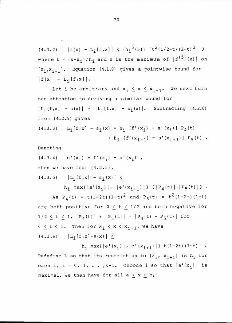
70

(4.3.2) jf(x) - Li[f,x] I .s_ (hi 5 /S!) Jt 2 (1/2-t) (1-tJ 2 j u

where t = (x-xi)/hi and U is the maximum of jf( 5 ) (x) I on

[xi,xi+l]. Equation (4.1.9) gives a pointwise bound for

jf(x) - Li[f,x] j.

Let i be arbitrary and xi~ x ~ xi+l" We next turn

our attention to deriving a similar bound for

Subtracting (4.2.6)

from (4.2.5) gives

(4.3.3) Li[f,x] - si(x) = hi [f'(xi) - s'(xi)] P 4 (t)

+ hi [f' (xi+ll - s' (xi+ll] P 5 (t)

Denoting

(4.3.4)

then we have from (4.2.5),

(4.3.5)

hi max(je'(xi)j, je'(xi+l)j} (jP 4 (t)j+JP 5 (t)j}.

As P 4 (t) = t(l-2t)(l-t) 2 and P 5 (t) = t 2 (1-2t)(l-t)

are both positive for 0 < t < 1/2 and both negative for

0 < t < 1. Then for xi ~ x ~ xi+l' we have

(4.3.6) jLi[f,x]-s(x) I .s_

hi max ( I e ' (xi) I , I e ' (xi+ 1 ) I } I t ( 1- 2 t) ( 1-t) I •

Redefine L so that its restriction to [xi, xi+ll is Li for

each i, i = 0, 1, •• ,k-1. Choose i so that je'(xi) I is

maximal. We then have for all a< x < b,

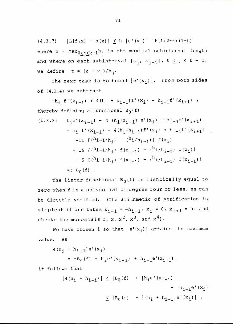
71

(4.3.7) IL[f,x] - s{x) I ~ h le' (xi) I Jt(l/2-t) (1-t) I

where h = max 0~j~k-lhj is the maximal subinterval length

and where on each subinterval [xj, xj+l], 0 ~ j ~ k - 1,

we define t = (x - xj) /hj.

The next task is to bound I e' (xi) I - From both sides

of (4.1.4) we subtract

-hi f' (xi-l) + 4(hi + hi_ 1 )f' (xi) - hi-lf' (xi+ll ,

thereby defining a functional B0 (f)

(4.3.8)

= hi f' (xi-1) - 4(hi+hi-l)f' (xi) + hi-1f' (xi+l)

-11 [(hi-1/hi) - (hi/hi-1)] f(xi)

+ 16 [(hi-1/hi) f(zi+ll - (hi/hi-l) f(zi)]

- 5 [(hi-1/hi) f(xi+ll - (hi/hi-l) f(xi_ 1 )]

=: B0 (f) •

The linear functional B0 (f) is identically equal to

zero when f is a polynomial of degree four or less, as can

be directly verified. (The arithmetic of verification is

simplest if one takes xi-l = -hi-l' xi = O, xi+l = hi and

2 3 4 checks the monomials 1, x, x , x , and x ).

We have chosen i so that le'(xi) I attains its maximum

value. As

4(h• + h- 1 )e'(x•) l 1- l

= -B 0 (fl + hie' (xi_ 1 ) + hi-le' (xi+ll,

it follows that

l4(hi + hi-1) I < IBo(f) I + !hie' (xi-1) I

+ lhi-1e' (xi) I

< IB 0 (f) I + I (hi+ hi_ 1 )e' (xi) I •

72

Hence

and

(4.3.9)

As Bo(f) is a linear functional which is zero for

polynomials of degree four or less, we can apply the Peano

theorem to get

(4.3.10) B0 (f) =

From (4.3.10) follows

xi+l (4.3.11) !B0 (f) I~ f !B0 [(x-y)+ 4 l I dy ui/ 4! •

xi-1

where Ui is the maximum of lf(S) I on [xi-l xi+l].

For xi-l ~ y ~ xi+l' B0 [(x-y)+ 4 l takes the form

( 4. 3 • 12) Bo [ ( x-y) + 4 ] =

- 16 (hi +hi-1) (xi-y) + 3 + 4hi-1 (Xi+l -y) 3

- 11 [ (hi-1/hi) - (hi/hi-l)] (xi - y) + 4

+ 16 [(hi-1/hi) (zi+l-y)+ 4 - (hi/hi-l) (zi-Y)+ 4

- 5 (hi-1/hi) (xi+l - y)4 •

In order to evaluate the integral of (4.3.11) we need

to know the sign behavior of B 0 [(x-y)+ 4 ]. We rewrite

(4.3.12) in a form which shows its symmetry about xi.

(4.3.13) Bo [ (x-y) + 4 J =

(hi/hi-1) [-S(xi-y) + hi-1) [(xi - y) - hi-1]3'

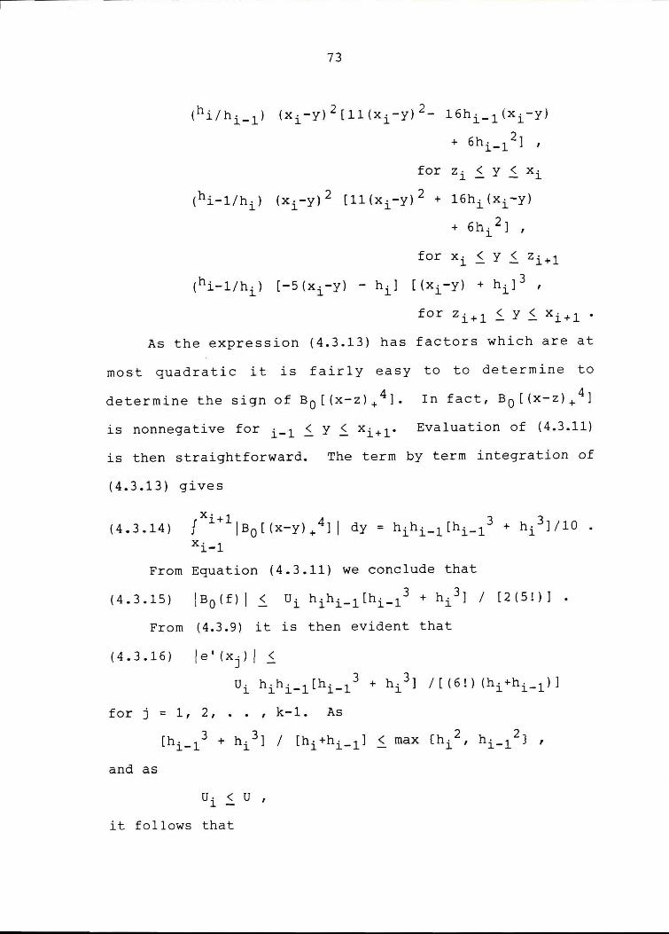
73

(hi/hi-1) (xi-y) 2 [11 (xi-y) 2_ 16hi-l (xi-y)

+ 6hi-l 2] ,

for zi .s_ y .s_ xi

(hi-1/h,) (x--y) 2 [ll(xi•-y) 2 + 16h,(x.-y) l l l l

+ 6hi 2] ,

for xi< y .S. zi+l

(hi-1/hi) [-5(xi-y) - hi] [(xi-y) + hi] 3 ,

for zi+l .S. y .S. xi+l.

As the expression (4.3.13) has factors which are at

most quadratic it is fairly easy to to determine to

determine the sign of B 0 [(x-z)+ 4 ]. In fact, B0 [(x-z)+ 4 1

is nonnegative for i-l .s_ y .S. xi+l" Evaluation of (4.3.11)

is then straightforward. The term by term integration of

(4.3.13) gives

(4.3.14) Xi+l f 1Bo[(x-y)+ 4 11 dy = hihi-l[hi-1

3 + hi

3]/10.

xi-1

From Equation (4.3.11) we conclude that

(4.3.15) IBo(f)I < U, h-h• 1 [h· 13 + h- 3 ] / [2(5!)] •

l l l- 1- l

From (4.3.9) it is then evident that

(4.3.16) le'(xj)I .S.

Ui hihi-l[hi-13 + hi3] /[(6!) (hi+hi-1)]

for j = 1, 2, , k-1. As

and as

ui .s. u ,

it follows that

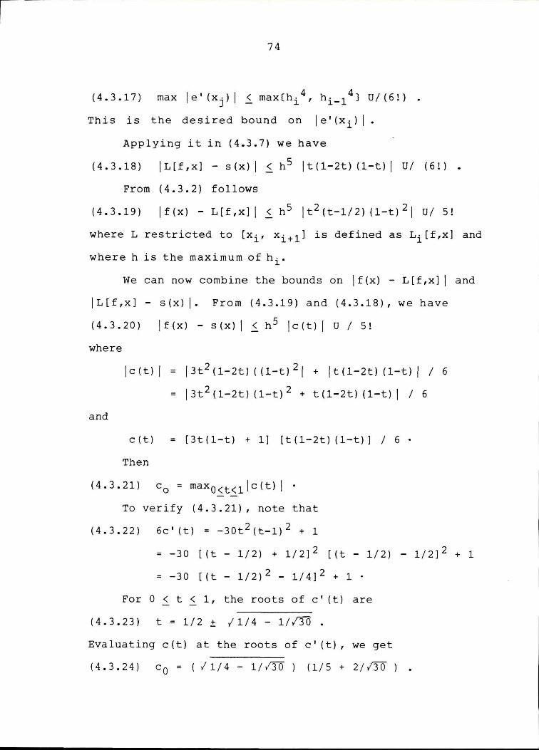
74

(4.3.17) max le' (xj) I .s_ max(hi 4 , hi_ 14 J U/ (6!) •

This is the desired bound on I e' (xi) I

Applying it in (4.3.7) we have

(4.3.18) IL[f,x] - s(x) I < h 5 it(l-2t) (1-t) I U/ (6!) •

From (4.3.2) follows

(4.3.19) lf(x) - L[f,x] I .s_ h 5 lt 2 (t-1/2) (1-t) 2 I U/ 5!

where L restricted to [xi, xi+l] is defined as Li[f,x] and

where h is the maximum of hi.

We can now combine the bounds on lf(x) - L[f,x] I and

IL[f,x] - s(x) I- From (4.3.19) and (4.3.18), we have

(4.3.20) lf(x) - s(x) I .s_ h 5 lc(t) I u / 5!

where

and

Jc(t) I = j3t2 (1-2t) ((1-t) 21 + jt(l-2t) (1-t) I / 6

= l3t 2 (1-2t) (1-t) 2 + t(l-2t) (1-t) I / 6

c(t) = [3t(l-t) + 1] [t(l-2t)(l-t)] / 6 •

Then

(4.3.21) c 0 = maxO<t<lic(t) I · To verify (4.3.21), note that

(4.3.22) 6c'(t) = -30t2 (t-1) 2 + 1

= -30 [(t - 1/2) + 1/2] 2 [(t - 1/2) - 1/2] 2 + 1

= -30 [(t - 1/2) 2 - 1/4] 2 + 1 ·

For 0 .s_ t .s_ 1, the roots of c' (t) are

(4.3.23) t = 1/2 .:t ✓ 1/4 - 1//30.

Evaluating c(t) at the roots of c' (t), we get

(4.3.24) CQ = ( /1/4 - 1//To) (1/5 + 2//3o) •

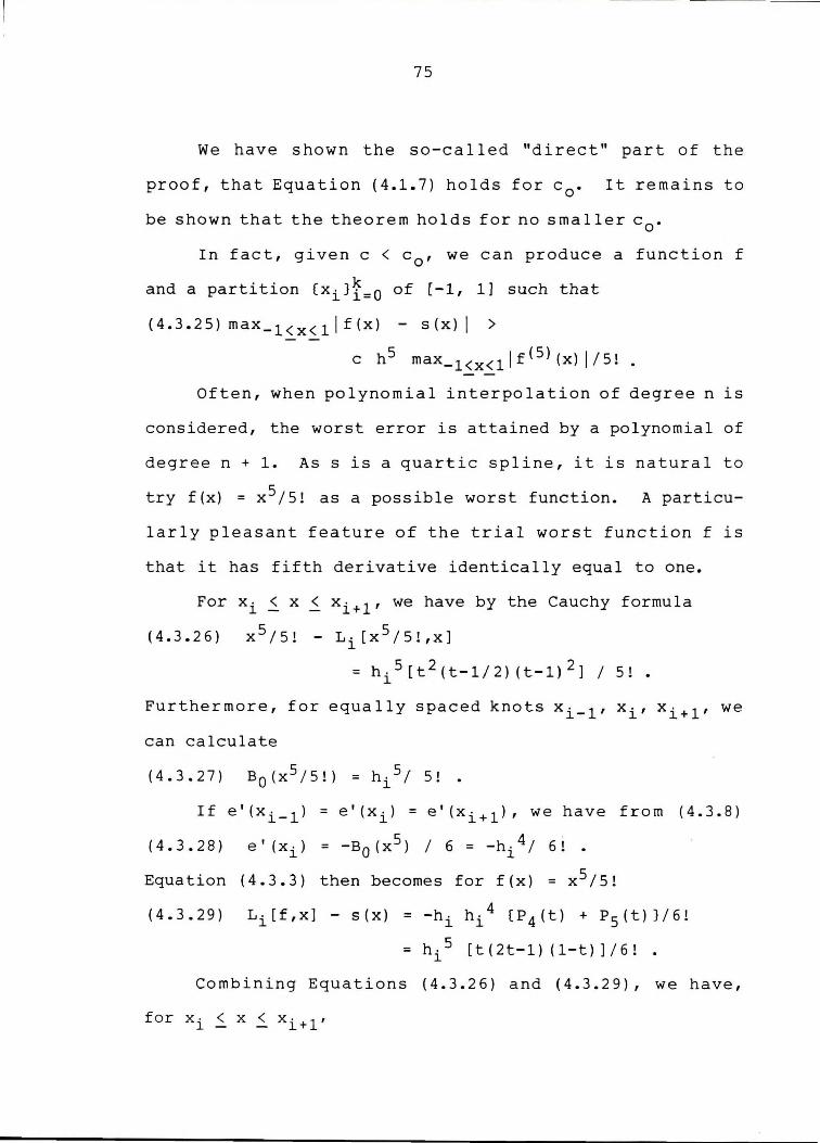
75

We have shown the so-called "direct" part of the

proof, that Equation (4.1.7) holds for c0

• It remains to

be shown that the theorem holds for no smaller c0

•

In fact, given c < c0

, we can produce a function f

. . ( }k and a partition xi i=0 of [-1, 1] such that

(4.3.25) max_l<x< 1 1 f (x) - s (x) I >

c h 5 max_l<x<llf(S)(x)j/5!.

Often, when polynomial interpolation of degree n is

considered, the worst error is attained by a polynomial of

degree n + 1. Ass is a quartic spline, it is natural to

try f(x) = x 5 /S! as a possible worst function. A particu­

larly pleasant feature of the trial worst function f is

that it has fifth derivative identically equal to one.

For xi< x < xi+l' we have by the Cauchy formula

(4.3.26) x 5 /S! - Li[x 5 /S!,x]

= hi 5 [t 2 (t-1/2)(t-1) 2 J / 5!.

Furthermore, for equally spaced knots xi-l' xi' xi+l' we

can calculate

(4.3.27) 5 _ 5 B0 (x /5!) - hi/ 5! .

If e' (xi_ 1 ) = e' (xi) = e' (xi+ll, we have from (4.3.8)

(4.3.28) e'(xi) = -Bo(x5 ) I 6 = -hi 4 / 6!.

Equation (4.3.3) then becomes for f(x) = x 5 /S!

(4.3.29) Li[f,x] - s(x) ""-hi hi 4 (P 4 (t) + P5 (t)}/6!

= hi 5 [t(2t-1) (1-t) ]/6!

Combining Equations (4.3.26) and (4.3.29), we have,

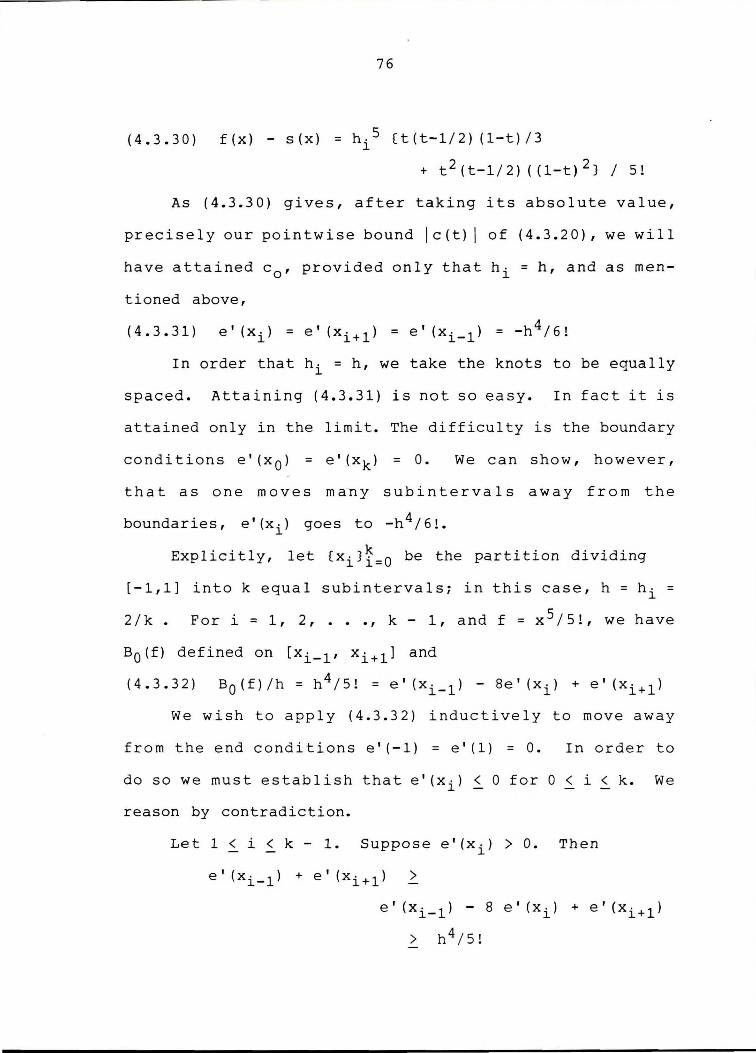
(4.3.30)

76

f(x) - s(x) = h , 5 [t(t-1/2) (l-t)/3 l

+ t 2 (t-1/2) ( (1-t) 2 } / 5!

As (4.3.30) gives, after taking its absolute value,

precisely our pointwise bound I c (t) I of (4.3.20), we will

have attained c0

, provided only that hi= h, and as men­

tioned above,

(4.3.31) e' (xi) = e' (xi+l) = e' (xi_ 1 ) = -h 4 /6!

In order that hi= h, we take the knots to be equally

spaced. Attaining (4.3.31) is not so easy. In fact it is

attained only in the limit. The difficulty is the boundary

conditions e' (x 0 ) = e' (xk) = O. We can show, however,

that as one moves many subintervals away from the

boundaries, e' (xi) goes to -h4 /6!.

Explicitly, let (xi}t=o be the partition dividing

(-1,1] into k equal subintervals; in this case, h =hi=

2/k. For i = 1, 2, ••• , k - 1, and f = x 5 /S!, we have

Bo(f) defined on [xi-l' xi+l] and

(4.3.32) Bo(f)/h = h 4 /S! = e' (xi-l) - Se' (xi) + e' (xi+l)

We wish to apply (4.3.32) inductively to move away

from the end conditions e' (-1) = e' (1) = O. In order to

do so we must establish that e' (xi) ~ 0 for O < i < k. We

reason by contradiction.

Let 1 < i < k - 1. Suppose e' (xi) > O. Then

e'(xi-1) + e'(xi+l) >

e'(xi_ 1 ) - 8 e'(xi) + e'(xi+ll

> h 4 /5!

77

Hence

max ( I e ' (xi_ 1 ) I , I e ' ( xi+ 1 ) I } > h 4 / [ 2 ( 5 ! ) 1 ,

contradicting the fact (4.3.17) that

h 4 / 6 ! > max ( I e ' ( xi_ 1 ) I , I e ' ( xi+ 1 ) I } • We have shown by assuming the contrary that

e' (xi) < 0 for i = 1, 2, •• , k - 1 •

Condition (4.1.3) is that e' (x 0 ) and e' (xk) are zero. Thus

(4.3.33) e'(xi) < 0 for i = 0, 1, •• , k.

and

Applying (4.3.32) again we have for i = 1, 2, •• , k - 1

Se' (xi) = -h4 /5! + e' (xi_ 1 ) + e' (xi+l) •

Ase' (xi_1 ), e' (xi+ll < 0, this implies that

Se' (xi) ~ -h4 /5!

(4.3.34) e' (xi)~ -h4 /[8(5!)] •

Similarly, for i = 2, 3, •• , k - 2, we have

Se' (xi) = -h4 /5! + e' (xi_ 1 ) + e' (xi+ll ,

and hence by (4.3.34),

e' (xi) < -h4 /5! - h 4 / [8 (5!)] - h 4 / [8 (5!)]

= -(1 + 1/4) h 4 /[8(5!)] •

Inductively, for i = j to i = k - j, we will have

e'(xi) < -(1 + 1/4 + 1/4 2 + • + l/4j-l}h4 /[8(5!)].

2 The harmonic series (1 + 1/ 4 + 1/ 4 + • . • is

equal to 1/(l - 1/4) or 4/3. Thus, in the limit as i, k,

and j go to infinity, we have

(4.3.35) e' (xi) ~ -(1/8) (4/3)h 4 /5! = -h 4 /6! •

We already know from (4.3.17) that ie'(xi) J ~ h 4 /6!. Thus

fork> 2j + 1, and k - j > i > j as j goes to infinity,

78

we have

{4.3.36) e' {xi) goes to -h4 /6! •

In the sense of (4.3.36), (4.3.31) is satisfied.

Then, goes x 5 /5! - s {x) goes

uniformly to the expression of (4.3.30) and (4.3.20) with

h = h ·• l It follows that the expression of (4.3.20)

cannot be improved further. In fact we have shown that

!c(t) I offers a pointwise exact bound, and its maximum c0

is the exact norm bound.

Proof of Theorem 4.2

We know from {4.3.1) that for xi < x .S. xi+l'

(4.4.1) s{x) - f{x) = P1 {t) f(xi) + P2 (t) f(zi+ll

+ P 3 (t) f{xi+l) + hi P 4 (t) s'{xi)

+ hi P 5 {t) s' {xi+l) - f(x) •

It is easily verified that P 1 (t) + P 2 (t) + P 3 {t) = 1.

Thus

(4.4.2) s(x) - f(x) = P1 (t) [f(xi) - f(x)]

+ P 2 (t) [f(Zi+l) - f{x)]

+ P 3 (t) [f{xi+l) - f(x)]

+his' {xi) P 4 (t)

+ hi s' {Xi+l) P 5 {t) •

Each of the first three terms on the right hand side

can be bounded in absolute value by (f,h). We also must

bound the last two terms. For equally spaced knots h = hi

= h • 1• i-, equation {4.1.4) reduces to

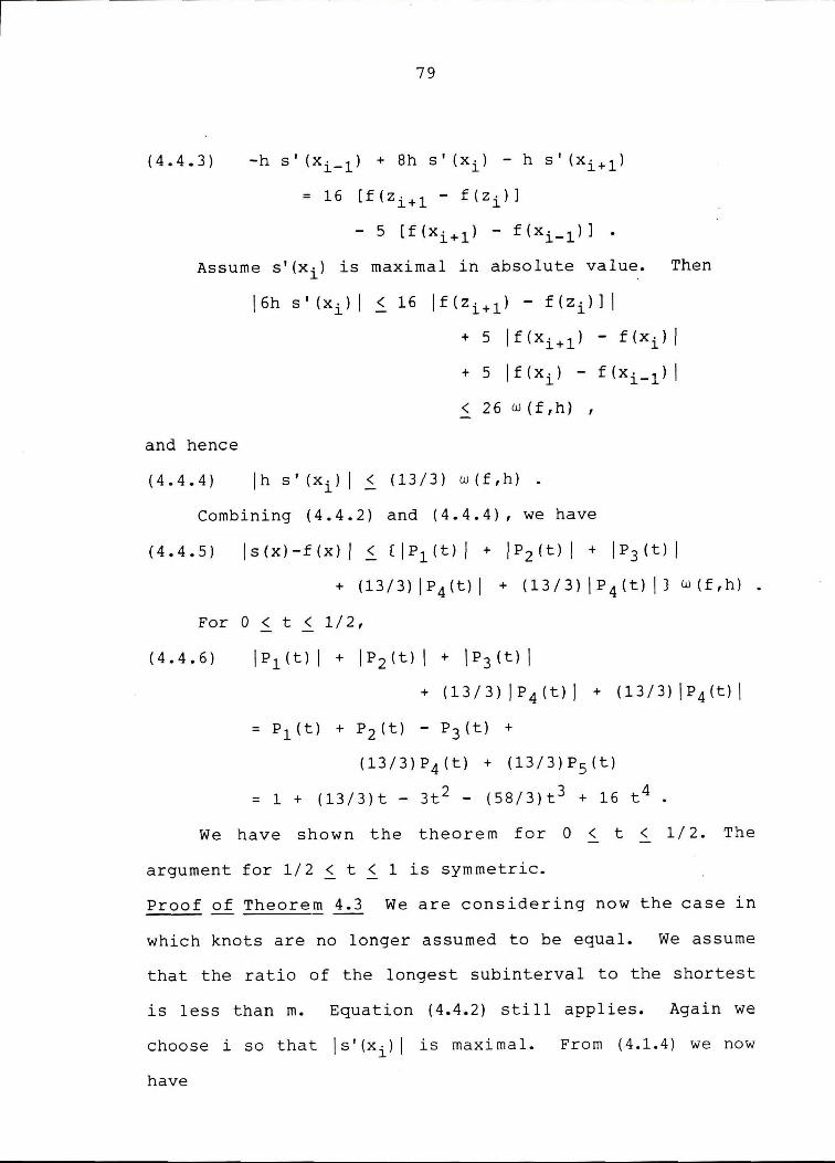
(4.4.3)

79

-h s'(xi_1 ) + 8h s'(xi) - h s'(xi+ll

= 16 [f(zi+l - f(zi)]

- 5 [f (xi+ll - f (xi_ 1 )] •

Assume s'(xi) is maximal in absolute value. Then

and hence

(4.4.4)

l6h s' (xi) I < 16 !f(zi+l) - f(zi)] I

+ 5 !f(xi+l) - f(xi) I

+ 5 !f(xi) - f (xi_ 1 ) I

< 26W(f,h),

lh s' (xi) I ~ (13/3) w (f,h) .

Combining (4.4.2) and (4.4.4), we have

(4.4.5) !s(x)-f(x) I~ [!P1 (t) I + IP 2 (t) I + IP 3 (t) I

+ (13/3)IP4(t)I + (13/3)IP4(t)!}W(f,h)

For O < t < 1/2,

(4.4.6) IP1 (t) I + IP2 (t) I + IP3 (t) I

+ (13/3)jP4(t)! + (13/3)IP4(tll

= P1 (t) + P2 (t) - P3 (t) +

(13/3)P4 (t) + (13/3)P 5 (t)

= 1 + (13/3)t - 3t2 - (58/3)t 3 + 16 t 4 .

We have shown the theorem for O < t < 1/ 2. The

argument for 1/2 ~ t ~ 1 is symmetric.

Proof of Theorem 4.3 We are considering now the case in

which knots are no longer assumed to be equal. We assume

that the ratio of the longest subinterval to the shortest

is less than m. Equation (4.4.2) still applies. Again we

choose i so that Is' (xi) I is maximal. From (4.1.4) we now

have

(4.4. 7)

Then

80

-his' (xi-1) + 4(hi+hi-1) s' (xi) - hi-ls' (xi+l)

= -11 [(hi-1/hi) - (hi/hi_1 )] f(xi)

+ 16 [ (hi-1/h ·) 1 f(zi+l) - (hi/hi-1) f (zi)]

- 5 [ (hi-1/h · ) f (xi+l) - (hi/hi-1) f(xi-1)] 1

= ll[hi/hi_1 ] [f(xi) - f(zi)]

+ 5[hi/hi-1] [-f(z•) + f(xi-1)] 1

+ ll[hi-1/hi] [f(zi+l) - f(X·)] l

+ 5 [hi-1/h ·] [f(zi+l) - f (Xi+l)] l

3 (hi + hi_ 1 ) Is' (xi) I < 16 hi/hi-l w (f, hi_ 1 /2)

+ 16 hi-1/hi w(f,hi/2)

and

ls'(xi)I < (16/3) [hi/hi-l + hi-1/hi] w (f,h)

h · + h· l 1 1-

where h = maxO<i<k-lhi.

Then for any given j, 0 .s_ j .s_ k-1 , and

m = max(hi}/(mini}, i = 0, 1, ••• , k - 1, we have

(4.4.8) rnax(lhj s'(xj)I, jhj s'(xj+illJ

< (16/3) h (m + 1/m) w (f,h) 2min[hi}

< (8/3) (m 2 + m) w (f,h) •

Substituting (4.4.8) into (4.4.2) yields the result

of the theorem.

CHAPTER FIVE IMPROVED ERROR BOUNDS FOR THE PARABOLIC SPLINE

Introduction and Statement of Theorems

The quartic splines of Chapter Four share and improve

many of the properties of the complete cubic spline. To

insure a good approximation to a given continuous

function, we must make the largest subinterval of a

partition small. Unfortunately, we must also pose some

additional restrictions on the partition. For instance,

in Theorem 4.3, the norm of the error depends not only on

the length h of the largest subinterval but also on the

ratio m of the largest to smallest length subinterval.

Similar additional restrictions must be made for the cubic

spline.

In this chapter, we will discuss a spline operator

for which the norm of the approximation error goes to zero

with the length of the largest subinterval, for any par­

tition and any continuous periodic function. This spline

is the piecewise parabolic spline introduced by Marsden

and discussed in Chapter One. Its properties are

summarized in Equations (1.6.1) to (1.6.7).

As Marsden points out, many of the bounds he gives

can be sharpened. The main result of this chapter will be

to accomplish this sharpening. While many of the bounds

81

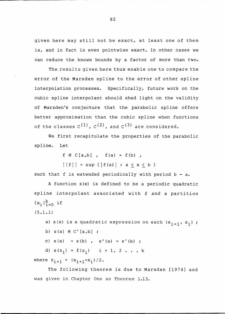
82

given here may still not be exact, at least one of them

is, and in fact is even pointwise exact. In other cases we

can reduce the known bounds by a factor of more than two.

The results given here thus enable one to compare the

error of the Marsden spline to the error of other spline

interpolation processes. Specifically, future work on the

cubic spline interpolant should shed light on the validity

of Marsden's conjecture that the parabolic spline offers

better approximation than the cubic spline when functions

of the classes c(l), c( 2 ), and c( 3 ) are considered.

We first recapitulate the properties of the parabolic

spline. Let

f e C[a,b] f(a) = f(b)

I If I I = sup ( If (x) I a<x<b}

such that f is extended periodically with period b - a.

A function s(x) is defined to be a periodic quadratic

spline interpolant associated with f and a partition

( }k i· f xi i=O

(5.1.1)

a) s (x) is a quadratic expression on each (xi-l' xi)

b) s(x) ec'[a,b];

c) s (a) = s(b) s'(a) = s'(b);

i = 1, 2 •• , k

where zi+l = (xi+l+xi)/2.

The following theorem is due to Marsden [1974] and

was given in Chapter One as Theorem 1.13.

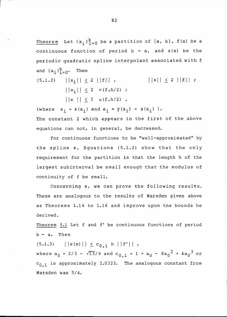
83

Theorem Let (xiJ1=o be a partition of [a, b], f(x) be a

continuous function of period b - a, and s (x) be the

periodic quadratic spline interpolant associated with f

and (xiJf=o· Then

(5.1.2) !!sill< 2 lltll,

I lei! I < 2 W(f ,h/2) ;

lie II< 3 w(f,h/2).

11s1I < 2 11£11;

(where S· = S(X·) and e- = y(x•) - S(X·) ). l l l l l

The constant 2 which appears in the first of the above

equations can not, in general, be decreased.

For continuous functions to be "well-approximated" by

the spline s, Equations (5.1.2) show that the only

requirement for the partition is that the length h of the

largest subinterval be small enough that the modulus of

continuity off be small.

Concerning s, we can prove the following results.

These are analogous to the results of Marsden given above

as Theorems 1.14 to 1.16 and improve upon the bounds he

derived.

Theorem 5.1 Let f and f' be continuous functions of period

b - a. Then

(5.1.3) lle(x)II .s_c 0 , 1 h 11£'11,

where a 0 = 2/3 - nJ/6 and c 0 , 1 = 1 + a 0 - 8a 02 + 4a 0

3 or

c 0 , 1 is approximately 1.0323. The analogous constant from

Marsden was 5 / 4.

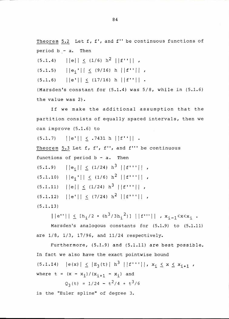
84

Theorem 5.2 Let f, f', and f" be continuous functions of

period b - a. Then

(5.1.4)

(5.1.5)

(5.1.6)

I Jell~ (1/6) h 2 llf"JI,

llei'II ~ (9/16) h llt"ll,

lle'II ~ (17/16) h 11£"11 • (Marsden's constant for (5.1.4) was 5/8, while in (5.1.6)

the value was 2).

If we make the additional assumption that the

partition consists of equally spaced intervals, then we

can improve (5.1.6) to

(5.1. 7) ile'II < .7431 h 11£"11 • Theorem 5.3 Let f, f', f", and f"' be continuous

functions of period b - a. Then

(5.1.9) Jleill ~ (1/24) h 3 llf'''II,

(5.1.10) llei'II ~ (1/6) h 2 llf"'ll,

(5.1.11) I/ell~ (1/24) h 3 Jlf'''II,

(5.1.12) Jle'II ~ (7/24) h 2 llf'''II,

(5.1.13)

I Je"I I< [hi/2 + (h3 /3hi 2 )] I If"'! I , xi_ 1 <x<xi.

Marsden's analogous constants for (5.1.9) to (5.1.11)

are 1/8, 1/3, 17/96, and 11/24 respectively.

Furthermore, (5.1.9) and (5.1.11) are best possible.

In fact we also have the exact pointwise bound

(5.1.14) Je(x) I ~ JE 3 (t) I h 3 I Jf' '' 11, xi~ x < xi+l ,

where t = (x - xi)/(xi+l - xi) and

Q3(t) = 1/24 - t 2 /4 + t 3 /6

is the "Euler spline" of degree 3.

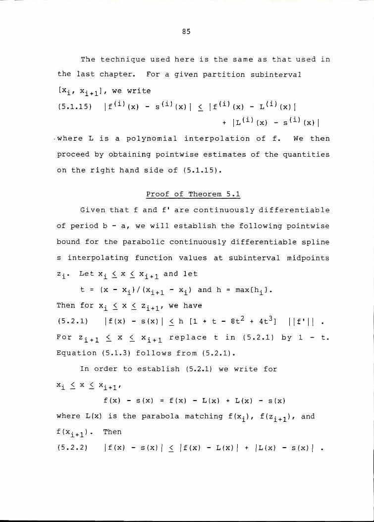
85

The technique used here is the same as that used in

the last chapter. For a given partition subinterval

(5.1.15) if(i)(x) - s(il(x)I < if(il(x) - L{il(x)I

+ IL(i) (x) - s(i) (x) I

-where Lis a polynomial interpolation of f. We then

proceed by obtaining pointwise estimates of the quantities

on the right hand side of (5.1.15).

Proof of Theorem 5.1

Given that f and f' are continuously differentiable

of period b - a, we will establish the following pointwise

bound for the parabolic continuously differentiable spline

s interpolating function values at subinterval midpoints

Then for xi< x < zi+l' we have

(5.2.1) If (x) - s (x) I _s. h [1 + t - 8t2 + 4t3 ] lit' 11 For zi+l < x < xi+l replace t in (5.2.1) by 1 - t.

Equation (5.1.3) follows from (5.2.1).

In order to establish (5.2.1) we write for

f(x) - s(x) = f(x) - L(x) + L(x) - s(x)

where L(x) is the parabola matching f(xi), f(zi+l), and

f(xi+ll. Then

(5.2.2) /f(x) - s(x) l < /f(x) - L(x) l + /L(x) - s(x) I •

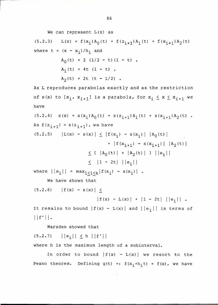
86

We can represent L(x) as

(5.2.3)

where t = (x - x , )/h• and l l

Ao ( t) = 2 ( 1 / 2 - t) ( 1 - t) ,

A1 (t) = 4t (1 - t) ,

A2 (t) = 2t (t - 1/2)

As L reproduces parabolas exactly and as the restriction

of s(x) to [xi, xi+ll is a parabola, for xi~ x ~ xi+l we

have

(5.2.5) IL(x) - s(x) I ~ Jf(xi) - s(xi) I IA 0 (t) I

+ Jf (xi+l) - s(xi+ll I JA 2 (t) I

< [ JA0 (t) I + JA2 (t) I } I Jeil I

< I 1 - 2t I I I ei 11

where I lei! I = maxl<i<kJf(xi) - s(xi) I

We have shown that

{5.2.6) Jf(x) -s(x)I <

Jf(x) -L(x)J + Jl- 2tl lleill •

It remains to bound Jf(x) - L(x)I and lleill in terms of

I If I I I •

Marsden showed that

(5.2.7)

where his the maximum length of a subinterval.

In order to bound If (x) - L {x) I we resort to the

Peano theorem. Defining g{t) =: f{xi+hit) = f(x), we have

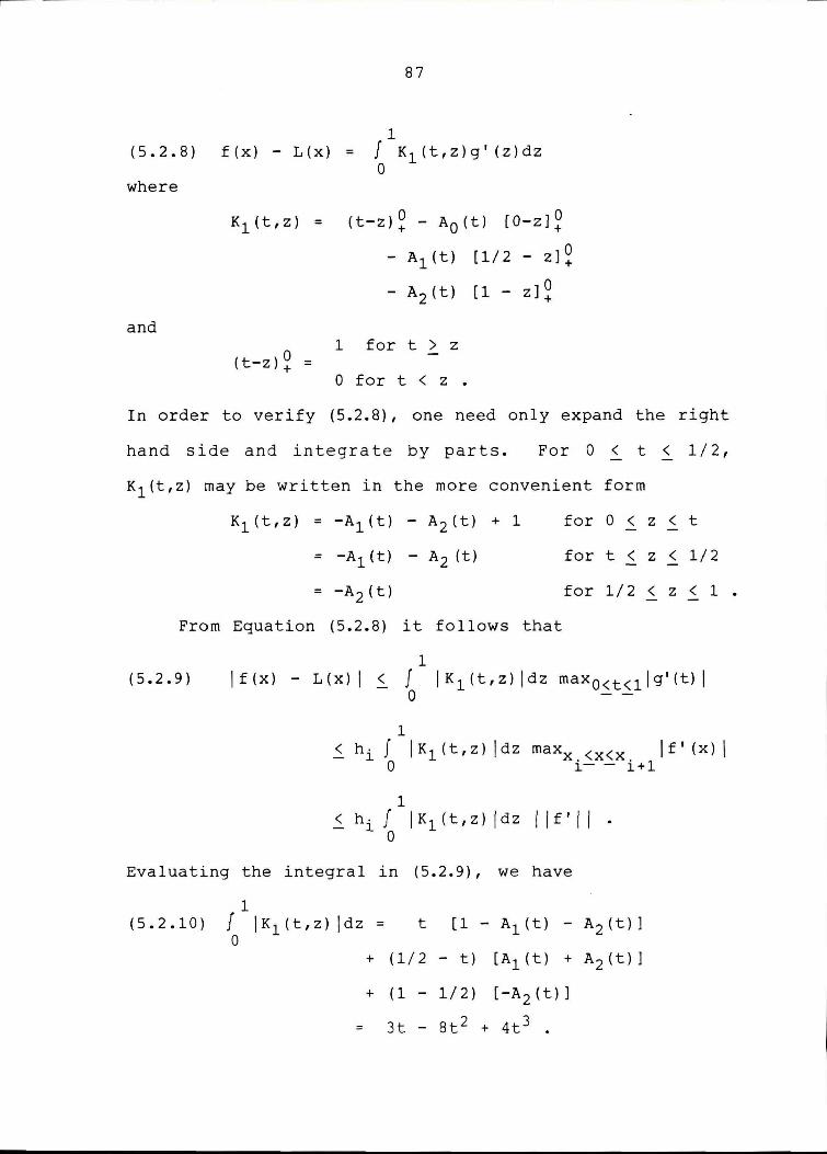
87

1 (5.2.8) f(x) - L(x) = f K1 (t,z)g' (z)dz

0 where

and

K1 (t,z) = (t-z)2 - A0 (t) (O-zJ2

(t-z)Z =

- A 1 (t) [1/2 - z]~

- A 2 ( t) [ 1 - z] 2

1 fort> z

O fort< z .

In order to verify (5.2.8), one need only expand the right

hand side and integrate by parts. For O < t < 1 / 2,

K1 (t,z) may be written in the more convenient form

From

(5.2.9)

K1 (t,z) = -A1 (t) - A2 (t) + 1 for 0 < z < t - -

= -A 1 (t) - A 2 (t) for t < z < 1/2 -

= -A 2 (t) for 1/2 < z < 1 - -Equation (5.2.8) it follows that

1 !f(x) - L(x)! < J !K 1 (t,z)!dz maxO<t<llg'(t)I

0

1 < hi J !K1 (t,z) !dz maxx <x<x If' (x) I

O i- - i+l

1 < hif IK1(t,z)ldz llf'I!.

0

Evaluating the integral in (5.2.9), we have

1 (5.2.10) f I K1 (t,z) !dz = t [1 - A 1 (t) - A 2 (t)]

0 + (1/2 - t) [A1 (t) + A 2 (t)]

+ (1 - 1/2) [-A2 (t)]

= 3t - Bt 2 + 4t 3 .

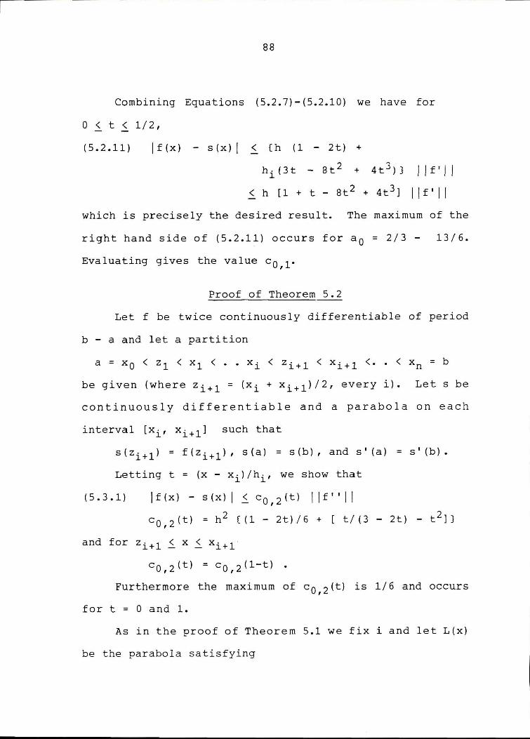
88

Combining Equations (5.2.7)-(5.2.10) we have for

0 < t .s_ 1/2,

(5.2.11) lf(x) - s(x)I < (h (1 - 2t) +

hi (3t - 8t 2 + 4t 3 ) J

< h [1 + t - 8t2 + 4t 3 ]

I If' 11

I If I 11

which is precisely the desired result. The maximum of the

right hand side of (5.2.11) occurs for a 0 = 2/3 - 13/6.

Evaluating gives the value c 0 , 1 •

Proof of Theorem 5.2

Let f be twice continuously differentiable of period

b - a and let a partition

a = XO < z 1 < X 1 < • • Xi < z i + 1 < Xi+ 1 <. • < xn = b

be given (where zi+l =(xi+ xi+l)/2, every i). Lets be

continuously differentiable and a parabola on each

interval [xi, xi+ll such that

s ( z i + 1 ) = f ( z i + 1 ) , s (a) = s ( b) , and s' (a) = s' ( b) •

Letting t = (x - xi)/hi, we show that

(5.3.1) lf(x) - s(x) I .S. c 0 , 2 (t) I If'' I I c 0 , 2 (t) = h 2 ((1 - 2t)/6 + [ t/(3 - 2t) - t 2 JJ

and for Zi+l .s. X .s. Xi+l

c 0 , 2 (t) = c 0 , 2 (1-t) •

Furthermore the maximum of c 0 , 2 (t) is 1/6 and occurs

fort= O and 1.

As in the proof of Theorem 5.1 we fix i and let L (x)

be the parabola satisfying

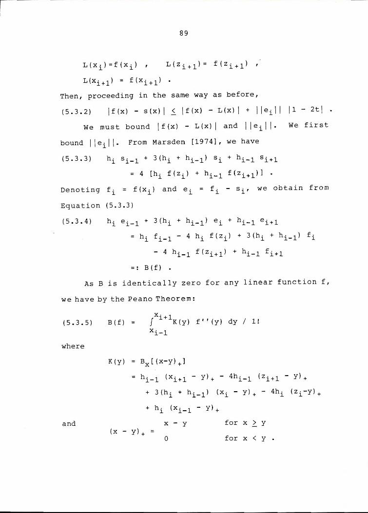
89

L(X·)=f(X · ) , l l

Then, proceeding in the same way as before,

(5.3.2) if(x) - s(x) I < if(x) - L(x) I + I lei\ I 11 - 2t\ •

We must bound If (x) - L (x) I and 11 ei I I• We first

bound 11 ei 11- From Marsden [1974], we have

(5.3.3) h, Si· -1 + 3(h • + h • 1l S· + h• l S · l l l 1- l 1- l+

Denoting fi = f(xi)

Equation (5.3.3)

and e. = f. - s. , l l l

we obtain from

(5.3.4) hi ei-1 + 3 (hi + hi-1) ei + hi-1 ei+l

= hi fi-l - 4 hi f(zi) + 3(hi + hi-l) fi

- 4 hi-1 f{zi+l) + hi-1 fi+l

-. B{f) •

As Bis identically zero for any linear function f,

we have by the Peano Theorem:

(5.3.5)

where

and

B ( f) = fxi+lK(y) f'' {y) dy / l!

xi-1

K (y) = Bx [ (x-y) +1

+ h• (x. 1 - Y)+ l i-

X - y for X > (x - y) + =

0 for X <

y

y .

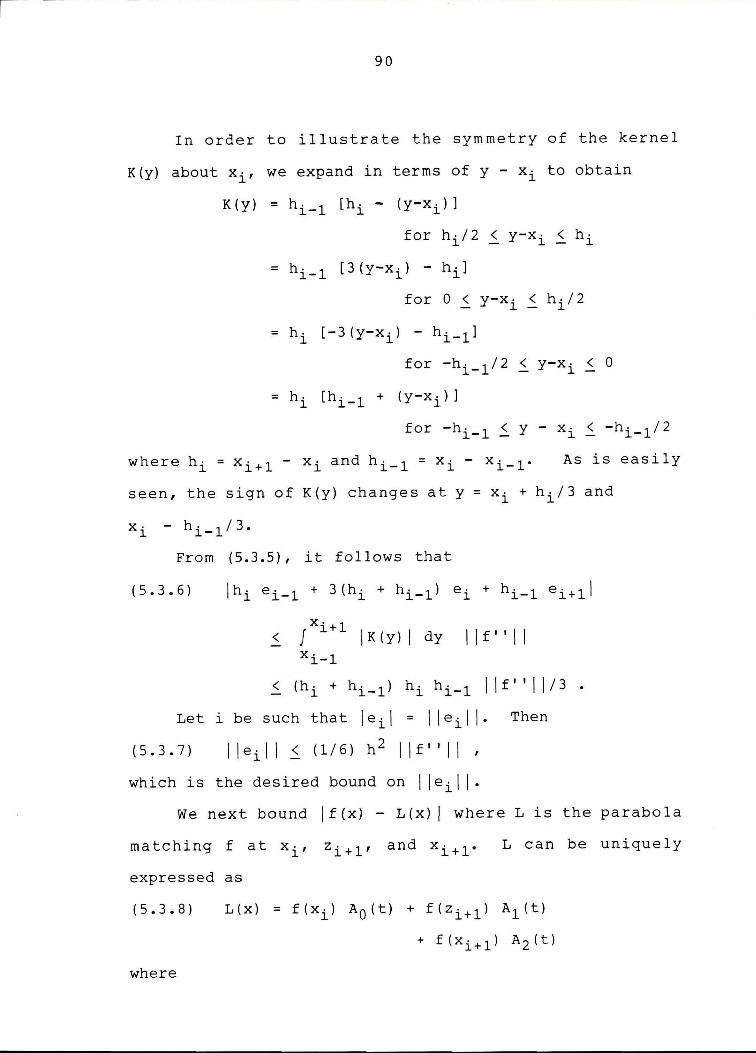
90

In order to illustrate the symmetry of the kernel

K(y) about xi, we expand in terms of y - xi to obtain

K(y) = hi-1 [hi - (y-xi)]

for hi/2 < y-xi < hi

= hi-1 [3(y-xi) - hi]

for O < y-xi < hi/2

= hi [-3(y-xi) - hi-1]

for -hi_ 1 ;2 < y-xi < 0

where h. = x. 1 - x • and h • 1 = x · - x • 1 . l l+ l l- l l- As is easily

seen, the sign of K(y) changes at y = x i+ hi/3 and

xi - hi-1/3.

From (5.3.5), it follows that

(5.3.6) lhl• ei•-1 + 3(hl• + hi•-1) e- + h- 1 e- 11 l l- l+

< Xi+l J JK(y) I dy I If II 11

xi-1

< (hi+ hi-1) hi hi-1 J if'' I l/ 3 •

Let i be such that Jeil = I Jeil J. Then

(5.3.7) lleill ~ (1/6) h 2 llf"II,

which is the desired bound on I Jeil J.

We next bound jf(x) - L(x) J where Lis the parabola

matching f at xi, zi+l' and xi+l" L can be uniquely

expressed as

(5.3.8)

where

L(x) = f(xi) Ao(t) + f(zi+l) Al (t)

+ f( x i+l) A2 (t)

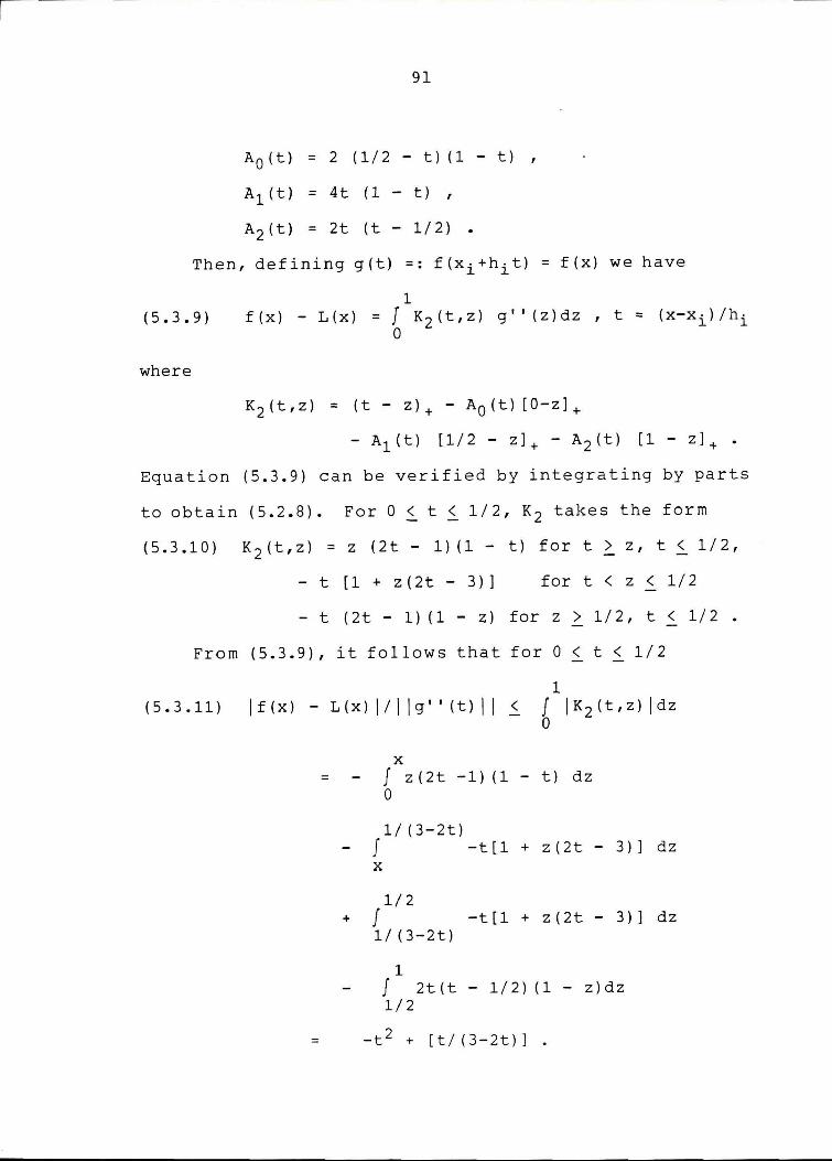
91

Ao ( t) = 2 ( 1 / 2 - t) ( 1 - t) ,

Al (t) = 4t (1 - t) ,

A2 (t) = 2t (t - 1/2)

Then, defining g(t) =: f(xi+hit) = f(x) we have

1 (5.3.9) f (x) - L(x) = J K2 (t,z) g'' (z)dz , t = (x-xi) /hi

0

where

K2 (t,z) = (t - z)+ - A0 (t) [O-z]+

- A1 (t) [1/2 - z]+ - A2 (t) [1 - z]+ •

Equation (5.3.9) can be verified by integrating by parts

to obtain (5.2.8). For O ~ t ~ 1/2, K2 takes the form

(5.3.10) K2 (t,z) = z (2t - 1) (1 - t) for t > z, t ~ 1/2,

- t [ 1 + z ( 2t - 3) ] fort< z < 1/2

- t (2t - 1) (1 - z) for z > 1/2, t < 1/2

From (5.3.9), it follows that for O < t < 1/2

1 (5.3.11) if(x) - L(x) Iii lg'' (t) 11 < J !K 2 (t,z) !dz -

0

X

= - J z(2t -1) (1 - t) dz 0

l/(3-2t) - J -t[l + z(2t - 3)] dz

X

1/2 + J -t[l + z(2t - 3)] dz

1/ (3-2t)

1 J 2t(t - 1/2) (1 - z)dz 1/2

= -t2 + [t/(3-2t)] .

92

Therefore , if O ~ t ~ 1/ 2, we have

(5.3.12) if(x) - L(x) Ii hi 2 [-t 2 + [t/(3-2t)]}j jf" (x) I I

We can now assemble the parts to get the pointwise bound

(5.3.1). Using the bound for if(x) - L(x)I of (5.3.11)

and the bound of (5.3.7) for I jeil I in the formula

lf(x) - s(x) I < if(x) - L(x) I + I leil I 11 - 2tl ,

we then have for O <ti 1/2,

(5.3.13) lf(x) - s(x)I i ( hi 2 [-t 2 + t/(3-2t)]

+ (1 - 2t) h 2 /6} llf"II

which, as hi i h, immediately implies (5.3.1). The result

for 1/2 < t ~ 1 follows by symmetry. It remains only to

be shown that the maximum of

O < c0

, 2 (t) = h 2 ((1 - 2t)/6 + [ t/(3 - 2t) - t 2 J}

is h 2 /6 and occurs fort= 0. To see this, expand c 0 , 2 (t)

at Oas

Co,2(t} = Co,2(Q) + t Co,2' (Q) + (t2/2) Co,2' I (y)

where O < t < 1/2 and O ~ y it. It is not hard to

verify that the last two terms of the above expression are

negative, and hence the maximum occurs at t = 0. This

completes the proof of Equation (5.1.4).

We next show Equation 5.1.5. From Marsden, we have

the tridiagonal system matching spline derivatives,

(5.3.14) h- l Si·-1' + 3(h - + h- 1l S·' + h- S · 1' l- l l- l l l+

or equivalently,

(5.3.15)

where

and the

93

h. 1 e • 1 ' + 3 (h. + h • 1 ) e • ' + h • e • 11

l- l- l l- l l l+

=: B1 (f).

B1 [ (x-y) +1 = h-l

= 8 (y-xi) - 3h-l

= 8(y-xi) + 3h - l i-

= -h. 1-l

last equality of (5.3.15)

2 i+l

X· l <

Z· l <

xi-1

can be

f. I l

.s_ y .s_ Xi+l

y < 2 i+l

y < X· l

<y < - z. l

verified by

integrating by parts and using the fact that B 1 is

identically zero if f is a linear function. From (5.3.15)

follows

(5.3.16) lh • le - 1 • + 3(h• + h, 1 ) e-' + h• e - 1 '1 l- 1- l i- l l l+

Xi+l < f I B 1 [ ( x-y) + 1 I dy I I f ' ' I I

xi-1

< (9/8) 2 2 (h · + h · l ) l l- 11£"11,

and hence

(5.3.17) llei'II .S. (9/16) h i!f"II,

which is precisely (5.1.5).

We next establish a pointwise bound on le'(t) I• We

show that for xi .S. x .S. xi+l' and t = (x - xi)/hi,

(5.3.18) lf'(x) - s'(x)I .S. ((9/16)h

+ 2 hi t(l - t)} llf"II.

94

If we maximize the right hand side of (5.3.18) by taking

hi = h and t = 1/2, then (5.1.6) is an immediate

consequence of (5.3.18).

To establish (5.3.18), we let J(x) be the unique

parabola satisfying

(5.3.19) = f I ( X. ) , ].

Then

and

J'(x• 1)= ].+

J' (x) - s' (x) = ( 1 - t)

(5.3.20) If' (x) - s' (x) I

e, I + ].

< lf'(x) - J'(x)I + IJ'(x) - s'(x)I

< lf'(x) -J'(x)I + llei'II (11-tl + lti}

< lf'(x) - J'(x)I + llei'II

As we already have an estimate for 11 ei' 11, we need

only estimate If' (x) - J' (x) I•

integration by parts that

1

It is easy to see by

(5.3.21) f' (x) - J' (x) = J K(t,z)g'' (z)dz / hi 0

where g(t) =: f(xi+hit) = f(x) and where

K ( t, z) = 1 - t for t > z

- t fort< z

From (5.3.21) follows

1 (5.3.22) lf'(x) - s'(x)I ~ f IK(z,t)idz llg''II / hi

0

and evaluation of (5.3.22) gives

95

(5.3.23) If' (x) - J' (x) I ~ hi 2t (1 - t) I If'' 11 .

Applying (5.3.23) and (5.3.17) in (5.3.20) gives

(5.3.24) If' (x) - s' (x) I ~

(hi 2t (1 - t) + (9/16) h } llf" 11 '

which is the desired pointwise bound.

In order to improve the bound for the case of evenly

spaced knots we return to the use of the parabola L

satisfying

L(xi) = f(xi), L(zi+l) = f(zi+ll ,

L(xi+ll = f(xi+l) •

Then for arbitrary i and xi< x < xi+l' we have

(5.3.25) If' (x) - s' (x) I

< lf'(x) - L'(x)I + IL'(x) - s'(x)I

< lf'(x) - L'(x)I

+ (1/hi) I ei Ao' (t) + ei+l A2' (t) I

< lf'(x) - L'(x)I

+ ( I ieil I/hi) ( !Ao' (t) I + IA2' (t) I}

where t = (x-xi)/hi. Differentiating equations (5.3.8)

gives

(5.3.26) I Ao' ( t) I = /3 - 4t/ I

I A2 I (t) I = 11 - 4t/

Recalling from Equation (5.3.7) that

I I ei 11 < (1/6) h2 !If"!/ I -we have

(5.3.27) /f'(x) - s'(x)/ ~ lf'(x) - L'(x)I

+ (h 2 /6hi) (/A 01 (t)/+/A2'(t)/} llf"i!

where

96

JA0 '(t)i + JA 2 '(tli = 4 - st, 0 < t < 1 / 4 - -= 2 1/4 < t < 3/4

= 8t - 4 , 3/4 < t < 1

To obtain a pointwise bound we need only bound

jf' (x) - L' (x) j. Differentiating (5.3.9), we obtain

(5.3.28) jf' (x) - L' (x) I .s_

h • l

1 J jK

2(l,O)(t,z)jdz jjf''(x)jj

0

where for O < t < 1/2

K2

(l,O) (t,z) = z(3 4t) t > z

- 1 + z(3 - 4t) t < z < 1/2

(1 - 4t) (1 - z) , 1/2 < z < 1 •

The only sign changes occur for z = 1/(3 4t) and

0 < t < 1/4 and along the lines t = 1/4 , z < 1/2, and

z = t. Evaluating the the integral of (5.3.28) for

0 .s_ t .s_ 1/4 then gives

(5.3.29) t 1

J I K2

(l,O) (t,z) jdt =

0 J z(3 - 4t)dz 0

1/ ( 3-4t) - J [-l+z(3-4t)]dz

t

1/2 + f [-l+z(3-4t)]dz

l/(3-4t)

1 +J (1-4t)(l-z)dz

1/2

= t 2 (3 - 4t) - 2t + 1/(3 - 4t) •

For the interval 1/4 < t < 1/2, the only sign change

is the 1 ine z = t. We obtain

{5.3.30)

97

1 X

f JK 2 {l,O) (t,z) ictt ==

0 J z(3 - 4t)dz 0

1/2 f [-1 + z(3-4t)]dz X

1 f {l - 4t) (1 - z)dz 1/2

= t 2 (3 - 4t) •

The expression of (5.3.30) is monotone increasing for

1/4 < t < 1/2. We have shown that

{5.3.31) if'(x) - L'(x)J/llf"II

<

hi (t 2 (3 - 4t) - 2t + 1/(3-4t)} ,

0 < t < 1/4

h · t 2 (3 - 4t) , l

1/4 < t < 1/2 .

Combining (5.3.27) and (5.3.31) we have

(5.3.32) if'(x) - s'(x)J!llf"II <

hi[t 2 (3-4t) - 2t + 1/(3-4t)]

+ (h 2 /3hi) (2-4t) ,

0 < t < 1/4

1/4 < t < 1/2 •

As usual these results can be extended by symmetry to

the interval 1/2 ~ t < 1. The bound given in (5.3.32) is

monotone decreasing from Oto 1/4 and increasing from 1/4

to 1/2. For an equally spaced partition, and t near 1/2,

(5.3.32) is quite a bit smaller than (5.3.23). For

instance for t = 1/ 2, we have 1/ 3 + 1/ 4 versus 1 7 / 16 from

(5.3.23). If we rewrite (5.3.23) as

98

(5.3.33) lf'(x) - s'(x)I < c 2 , 1 (t) llf''II

where

c2 , 1 (t) = hi 2t (1 - t) + (9/16) h

and write (5.3.32) as

(5.3.34) If' (x) - s' (x) I ~ c 2 , 1 (t) I If'' 11

where c 2 , 1 (t) is the right hand side of (5.3.32), then we

have also the pointwise bound

(5.3.34) lf'(x) - s'(x)I ~

min(c 2 , 1 (t), c 2 , 1 (t)) llf"II.

For h = h-, the maximum of the right hand side of (5.3.34) l

is approximately .7431 h I Jf" 11 and occurs for t

approximately equal to .10038.

This completes the proof of Theorem 5.2.

Proof of Theorem 5.3

We first show that if f, f', f", and f'" are

continuous and of period b - a, then

(5.4.1) llf - s!I < (1/24) h 3 llf"'II wheres is the parabolic and periodic (once differen­

tiable) spline interpolating subinterval midpoints.

Furthermore, "1/24" cannot be improved.

We proceed by demonstrating (5.1.14). For a given

partition and subinterval [xi, xi+ll, we write

(5.4.2) Jf(x) - s(x) I < Jf(x) - L(x) I + JL(x) - s(x) I where L(x) is the unique parabola satisfying

(5.4.3) L(xi) = f(xi) , L(zi+ll = f(zi+ll ,

L(xi+ll = f(xi+l)

99

L(x) may be uniquely

expressed as

(5.4.4)

where t

L(x) = f(xi) A0 (t) + f(zi+l) A1 (t)

+ f(xi+l) A 2 (t)

= (X - X · ) /h · , l l

A0 (t) =

A1 (t) =

A2 (t) =

and

2(1/2

4t(l -2t(l/2

- t) (1 - t) ,

t) ,

- t)

Proceeding by using the Cauchy formula one obtains

(5.4.5} if(x) - L(x) I ~

(1/6) lt(l/2 - t)(l - t)i IJf'''li •

In order to bound

(5.4.6) IL(x) - s (x) I = [f(xi) - s(xi)] A0 (t)

+ [f (Xi+l) - s (Xi+ll] A2 (t)

< lleill [ JAo(t)J + IA2(t)I J

= I ieil I 11 - 2tl ,

we must bound J JeiJ I = maxj=l, 2 •• ,k(lejlJ where

ej = f(xj) - s(xj). To bound I Jeil I, we resort in turn to

the tridiagonal system of (5.3.4),

(5.4. 7) h• ei-1 + 3(h · + hi-1) e- + h • 1 ei+l l l l 1-

= h-f• l - 4h. f (z.) + 3(h • + h • 1 ) f · l 1- l l l 1- l

- 4hi_ 1f(zi+ll + hi-lfi+l

- . B1 (f)

B1 (f), so defined, is a linear functional identically

zero for polynomials of degree two or less. We thus have

(5.4.8)

where

B1(f) = JXi+lK(y)f"' (y)dy / 2!

xi-1

Then

100

K (y) = Bl [ (x-y) + 2 ]

= hi-1 [xi+l - y]~ - 4hi-1 [ zi+l - y]~

+ 3(h• + h, 1 ) [x• - yJ+ 2 J. i- l

- 4hi [zi - y]i + hi-1 [xi-1 - y]~

2 = hi-1 [hi - (y-xi)] , hi/2 ~ y-xi ~ hi

2 2 hi-1 [hi - (y-xi)] - 4hi-1 [hi/ 2 - (y-xi)]

0 ~ y-xi < hi/2

-hi[hi-1 + (y-xi)2] + 4hi[hi-1/2 + (y-xi)]2 ,

-hi-l/2 ~ y-xi ~ 0

(5.4.9) lh•e • 1 + (h• + h • 1 )e • + h, 1 e - 1 1 l l- l J.- l J.- l+

Xi+l < f I K ( Y) I dy I If' ' ' I I / 2 !

xi-1

= (1/12) (hi-lhi 3 + hihi-13

) llf"'II

If we take i so that lei! is maximal, then we have

(5.4.10) 2(hi + hi_ 1 ) I lei! I <

= (1/12) (hi-lhi 3 + hihi-1 3 ) llf"'II

and hence

(5.4.11) I lei! I

< (1/24) (hi-lhi 3 + hihi-1 3 )/(hi+hi-l) I If"' 11

< (1/24) h 3 llf"'II ·

Combining (5.4.6) and (5.4.11), we have

(5.4.12) lf(x) - s(x) I ~ lf(x) - L(x) I + I lei! I 11 -2tl

< [jt(l/2-t)(l-t)j/6 + {1/24)jl-2tj}h3 11f"'II

= IQ3(t)I h 3 llf"'II

where Q3(t) is the Euler spline of degree three. Equation

101

(5.4.12) is precisely (5.1.14).

(5.1.9) and (5.1.11).

From it follow also

To see that (5.1.14) cannot be improved, consider the

"Euler spline" Qn(x) constructed by integrating a constant

n times so that the nth integration is odd for n odd and

even for n even. On the unit interval, the first few

Euler splines are

(5.4.13)

Ql(X) = X - 1/2 ,

Q2 (x) = x 2 /2 - x/2

Q3(X) = x 3 /6 - x 2 /4 + 1/24 . These can be compared to the even Euler polynomials given

in Chapter Two.

If we extend the Euler splines to the real line by

setting

( 5. 4 . 14) Qn ( x) = ( -1) j Qn ( t + j )

0 < t < 1 and j integer, then Qn(x) is n - 1 times

continuously differentiable and piecewise n times

continuously differentiable. Qn is of period 2 and has

nth derivative of plus or minus one. Q is thus a member n

of the class of functions with nth derivative piecewise

differentiable. The third derivative of o3 can be repre­

sented as the pointwise limit of the the third derivative

of a sequence [fi} of three times continuously differen­

tiable functions which converge uniformly to o3. Further­

more each of the fi have third derivative bounded in

absolute value by one.

102

Restricting Q3 (x) to any interval [0, 2k], consider

the once continuously differentiable splines parabolic in

each interval [i, i+l], and satisfying

(5.4.15) S(Zi+l) = O3(Zi+l) = 0 ,

s(0) = s(2k) , s' (0) = s' (2k)

The spline s thus defined is identically zero. It is not

hard to see that the maximum error occurs at the integer

knots and is 1/24. In fact we have shown that Q3 (x) is

actually a pointwise exact bound.

We next demonstrate Equation (5.1.10),

(5.1.10) llei'II i (1/6) h 2 llf"'II ,

uses the same functional B1 that we used in proving

(5.1.5). As in that case we have

f. I l

which is identically zero for all polynomials of degree

two or less. Hence

(5.4.17) IB1(f)I <

where

+ 6(h· + h, 1 )(y-x-) l 1- l +

+ 2h , 1 (y-x. 1 ) 1- 1- +

---- - ------ ---- --- - - - - - - - - - -

103

= 2h - 2 - 2h · (y-x-) l l l

hi/2 ~ y-xi < hi

2 6hi(y-xi) - 8(y-xi) ,

0 ~ y-xi ~ hi/2

-6hi-l(y-xi) - 8(y-xi)2 ,

-hi_ 1 /2 ~ y-xi < 0

2 2hi-1 + 2hi-1 (y-xi) ,

-hi-1 ~ y-xi ~-hi-1 12 •

Conveniently, the above kernel is positive. Evaluation of

the integral in (5.4.17) is thus straightforward, leading

to

(5.4.18) lhi-1 ei-11

+ 3 (hi + hi-1) ei' + hi ei+l1

I

< (1/3) (hi 3 + hi-1 3 ) I If' 11

) I-Assuming that i is such that lei'I attains its maximum we

then have

3 3 (5.1.10) 11ei 1 11 < (hi + hi-1 ) I If I I I 11

6 (hi+ hi-1)

~ (1/6) h2 I If' II II .

In order to extend the bound (5.1.10) to the entire

interval, choose any subinterval [xi, xi+l] of the given

partition and consider the line J' interpolating fi' and

fi+l'· J' may be represented as

(5.4.19) J' (X) = (1 - t) fi' + t fi+l' .

By the triangle inequality, we have

(5.4.20) If 1 (x) - s 1 (x) I ~ If 1 (x) - J 1 (x) I

+ IJ'(x) - s'(x)I.

As f' is twice continuously differentiable, we have the

well-known inequality

104

(5.4.21) lf'(x) - J'(x)! .s_ hi 2 t(l - t) llf'''II / 2!.

As both J' ands' are lines on [xi, xi+l], we have

(5.4.22) IJ' (x) - s' (x) I .s_ [fi' - si'] (1 - t) +

[fi+l 1 - si+1'] t

< I I ei' I I ( I 1 - t I + It I }

< I I ei' 11

< (1/6) h 2 llf"'II •

Adding (5.4.21) and (5.4.22) gives the desired formula

(5.4.23) lf'(x) - s'(x)I < [1/6 + t(l-t)/2] h 2 llf'"II

< (7/24) h 2 !lf'"II •

Several further refinements of this argument are possible.

This particular bound may be worthy of further study in

the future.

We next wish to bound f''(x) - s''(x). Choosing the

arbitrary partition subinterval [xi, xi+l], we consider

the parabola L matching fat xi, zi+l' and xi+l" By the

triangle inequality we have

(5.4.24) If" (x) - s" (x) I

< lf"(x)-L"(x) I + jL"(x) -s"(x) I

< lf"(x) - L"(x)I

+ (l/hi2) lei Ao'' (t) + ei+l A2'' (t) I

< lf''(x) - L''(x)I

+ (l/hi2) lleill (IAo"(t)l+IA2"(t)IJ

< If'' (x) - L'' (x) I

+ (l/hi 2 ) (h 3 /24) I If" I 11 [4 + 4]

< /f"(x) - L"(x)/ + (h 3 /3hi 2 ) /lf"'/1

The bound on f'' (x) - L'' (x) is obtained by the Peano

105

theorem technique. We have for 0 < t < 1 and -

f e C'" [xi,xi+lJ' that

(5.4.25) If' ' (x) - LI I (X) I <

1 h•

l IK( 2 ,0) (t,z) jdz llt"'ll/21

0

where

K(t,z) = (t - z)~ - A 0 (t) (0 - zJ2 +

- A 1 ( t) (1/2 - z]~ - A 2 (t) [1 - zJi

= (t - z) 2 - (1/2 - z) i 4t(l - t) +

- (1 - z) 2 2t(t - 1/2)

and for 0 < t < 1/2,

K( 2 ,0) (t,z)/2! = 2z 2 t > z

-1 + 2z 2 t < z' z < 1/2

- 2(1 - z)2 t < z' z > 1/2 . The first of these two terms is positive and the last two

are negative. Evaluation of the integral of (5.4.25) is

straightforward, giving for O < t < 1/2,

(5.4.26) 1£" (x) - L" (x) I ~

hi ((4t 3 /3) -t+ 1/2] llf"'II.

Using (5.4.26) in (5.4.24) gives for O ~ t ~ 1/2,

(5.4.27) 1£'' (x) - s'' (x) I ~ (hi[ (4t 3 /3) - t + 1/2]

+ h3/3hi2] I If' I I 11

~ (hi/2 + h3/3hi2} I 1£' I I 11 '

which holds also for 1/2 < t < 1.

Using the linear interpolation of fi' and fi+l' and

the usual triangular inequality, we may obtain the

alternate estimate

106

(5.4.28) . jf'' {x) - s'' {x) I < (hi[l/2 + t(l - t) l

+h2/3hi} llf'''II

which when h is larger than hi sometimes offers a lower

estimate of the error. As the proof is very similar to

those already given, we omit the details.

CHAPTER SIX CONCLUDING REMARKS

In the above chapters, we have given bounds for the

error of approximation of several polynomial and spline

interpolations. Rather than restate the theorems proved

in previous chapters, we will try to indicate what further

work is possible and desirable.

The work done here has provided some of the

motivation for the work of Bojanov and Varma (in

preparation) extending Cauchy's formula for the error of

polynomial interpolation to an expression for derivative

error. They proved the following theorem.

Theorem 6.1 (Bojanov and Varma) Let f e c(n+l) [a,b] and

let L [f ,x] be the polynomial of degree n interpolating f

at n + 1 points. Then for i < n + 1, we have

(6 .1.1) lf(i) (x) - L(i) [f,x] I _s.

11 n+l (i) 11 I If (n+l) 11/ (n+l) !

where n

n+l(X) = (X - xi) • i=O

Furthermore, (6.1.1) continues to hold for the case of

Hermite interpolation (when n (x) is appropriately

redefined). In particular, let f e c( 2 m) [0,1) and let

v 2 m-l by the two-point Hermite interpolation satisfying

107

108

V 2m- l { 0) = f { 0) ,

V2m-l {i) (0) = f{i) (0)

for i = 1, 2, • • , m - 1. Then

(6.1.2) lf{i) {x) - v2m-1 {i) {x) I

V 2m-l ( 1) = f { 1) ,

V2m-l {i) (1) = f {i) (1) ,

~ I ldi xm{l-x)ml I I lf{ 2m) I l/{2m) ! •

dxi

Equation (6.1.2) generalizes the results of Birkhoff and

Priver [1967]. A further generalization of (6.1.1) could

hold for well-posed two-point Birkhoff interpolation and

thus give the norm bounds of Chapters Two and Three.

An alternate approach, suggested in conversation with

Garrett Birkhoff, is to compute pointwise bounds for the

derivatives of polynomial interpolation by the automated

approximate evaluation of Peano kernels. A computer

routine that accomplishes the necessary evaluations is

given by Howell and Diaa {available on request). Similar

routines could automate some other sorts of error bounds.

Some of the possibilities are detailed in Howell and Diaa.

We next discuss further possibilities for the study

of spline error bounds. Hopefully, knowledge of the errors

of such error bounds should aid in comparing various

spline operators. For instance, for the class of

functions three times continuously differentiable, the

periodic parabolic splines were shown in Theorem 5.3 to

have bounds very close to the cubic splines of the type

discussed by Varma and Katsifarakis {Theorem 1.17). On

the other hand, many of the parabolic spline bounds can be

109

bettered by a c( 2 ) quartic spline which will be discussed

in 1 a ter work.

Many other spline error bounds may be amenable to the

same techniques employed here. Among these are the

derivative bounds for the c( 2 ) quartic spline of Chapter

Four, bounds for the lacunary quintics discussed by Meir

and Sharma [1973], and bounds for the local scheme

proposed by Prasad and Varma [1979].

Even the extensively studied cubic splines require

further study along these lines. The techniques used here

might yield good results when the interpolated functions

are once or twice continuously differentiable. Even the

second derivative bound given by Hall and Meyer [1976] for

c( 2 ) cubic splines interpolating c( 4 ) functions

differentiable is not exact. Finally of course it would

be of interest to develop a method (even if merely

numeric) of deriving optimal bounds for spline

interpolation in each case that the problem makes sense.

Another type of error problem which is accessible by

techniques similar to the ones given here is the error of

the quadrature associated with any given piecewise

polynomial interpolation.

REFERENCES

Ahlberg, J. H., and Nilson, E. N. "The approximation of linear functionals." J. SIAM Numer. Anal. 3:173-182 ---(1966).

Ahlberg, J. H., Nilson E. N., and Walsh J. L. The Theory of Splines and their Applications. Academic Press, New York (1967).

Atkinson, A. K. E. "On the order of convergence of natural cubic spline interpolation problems." SIAM ~ Num. Anal. 2:89-101 (1968).

Bernstein, S. approximation deg re donne. II

(1912).

N. "Sur l'ordere de la meillure des fonctions continues par des polyn6mes de M em • Ac ad . de Be 1 g i q u e 2 m e Serie 4 : 1-1 0 4

Birkhoff, G. D. "General mean value and remainder theorems with applications to mechanical differentiation and integration." Trans. Amer. Math. Soc. 7:107-136 (1906).

Birkhoff, G., and DeBoor, c. "Error bounds for spline interpolation." ~ Math. Mech. 13 :827-836 (1964).

Birkhoff, G., and Priver, A. "Hermite interpolation errors for derivatives." J. Math. Phys. ~:440-447 (1967).

Cheney, E. w., and Schurer, F. "A note on the operators arising in spline approximation." J. Approx. Theory !:94-102 (1968).

Ciarlet, P. G., Schultz, M. H., and Varga, R. S. "Numerical methods of high-order accuracy." Num. Math. 2_:394-430 (1967).

Davis, P. J. Interpolation and Approximation. Dover, New York (1975).

De Boor, C. A Practical Guide to Splines. Springer­Verlag, New' -York (1978).

110

111

Dzjadyk, V. K. "Constructive characterization of functions satisfying the Lip a condition O < a < 1 on a finite segment of the real axis." Izv. Akad. Nahk. Sov. ~at. 2: 623-652 (1956).

Fejer, L. "Uber interpolation." ~ttinger Nachrichten 66-91, Akademie der Wissenschaften, G~ttingen, (1916).

Golub, G. H., and Van Loan, C. F. Matrix Computations. Johns Hopkins University Press, Baltimore, Md. (1983).

Hall, C. A. "On error bounds for spline interpolation." ~Approx.Theory l:_:209-218 (1968).

Hall, C. A., and Meyer, W. w. "Optimal error bounds for cubic spline interpolation." J. Approx. Theory .l.§_:105-122 (1976).

Howell, G., and Diaa, N. "An APL Routine for Calculating Birkhoff Error Bounds." available on request (1986).

Jackson, D. The Theory of Approximation. Amer. Math. Assoc., New York (1930).

Karlin, S. Total Positivity, 2 Vols. Stanford University Press, Stanford, Calif. (1968).

Lidstone G. J. "Notes on the extension of Aitken's theorem (for polynomial interpolation) to the Everett types." Proc. Math. Soc. Edinburgh ~:16-19 (1930).

Lorentz, G. G. Birkhoff Interpolation. Addison-Wesley, Reading, Mass. (1983).

Lucas, T. R. "Error bounds for interpolating cubic splines under various end conditions." SIAM J. Numer. Anal. ---11:569-584 (1974).

Marsden, M. J. "On uniform spline approximation." ~ Approx. Theory _§_:249-253 (1972).

Marsden, M. J. "Quadratic spline interpolation." Bull. Amer. Math. Soc. 80:903-906 (1974).

Meir, A., and Sharma, A. "On uniform approximation by cubic splines."~ Approx. Theory ~:270-274 (1969).

Peano, G. "Resto nelle formule di quadratura espresso con un integrale definite." Rend. Accad. Lincei 22:562-569 (1913).

Powell, M. J. D. Approximation Theory and Methods. Cambridge University Press, New York (1981).

112

Sard, A. Linear Approximation. Amer. Math Soc., Providence, R.I. (1963).

Schoenberg, I. J. "Contributions to the problem of approximation of equidistant data by analytic functions. Part A: On the problem of smoothing or graduation. A first class of analytic approximation formulas." Quart. Appl. Math. _!:112-141 (1946).

Schoenberg, I. J. "On interpolation by spline functions and its minimal properties." Internat. Series Num. Math. {Birkh~ser) 1:109-129 {1964a).

Schoenberg, I. J. "Spline interpolation and best quadrature formulae." Bull. Amer. Math. Soc. 2..Q_:143-148 (1964b).

Schoenberg, I. J. "On Hermite-Birkhoff interpolation." ~ !:!ath. Anal. Appl. 16:538-543 (1966).

Sharma, A., and Meir, A. "Degree of approximation of spline interpolation." ~ Math. Mech. 15:759-767 (1967).

Stroud, A. H. Numerical Quadrature and Solution of Ordinary Differential Equations. Springer-Verlag-,-New York (1974).

Timan, A. F. "Approximation of functions satisfying Lip conditions." Dok. Akad. Nahk. Sci. SSSR. 77:969-972 (1951).

Varma, A. K., and Katsifarakis, K. L. "Optimal error bounds for cubic spline interpolation." in Approximation Theory and Applications, Proc. Int. Conf. 75th Birthday G. G. Lorentz, St. John's, Newfoundland Res. !:!ath. 133 (in press).

Walsh, J. L., Ahlberg, J. H., and Nilson E. N. approximation properties of the spline fit." J. Mech. 11:225-234 (1962).

"Best Math.

Whittaker, J. M. "On Lidstone's series and two-point expansions of analytic functions." Proc. London Math. Soc. 431-469 (1934).

Widder, D. V. "Completely convex functions and Lidstone s e r i e s . " Tran s • ~~ e r • !:! a th . Soc . ~ : 3 8 7 - 3 9 8 ( 1 9 4 2 ) .

Zygmund, A. Trigonometric Series, Vol. 1. Cambridge University Press, Cambridge, England (1968).

BIOGRAPHICAL SKETCH

The author was born on November 9, 1951, in Winfield,

Kansas. He graduated from high school in Emporia, Kansas,

in 1969 and received his B. A. in mathematics from New

College in Sarasota, Florida, in 1973. After graduation,

he worked as a construction estimator in the Washington,

D.C., area. He entered graduate school in 1978 and

received an M.S. in mathematics in 1981, an M.S. in

engineering sciences in 1984, and a Ph.D. in mathematics

in 1986.

113

I certify that I have read this study and that in my opinion it conforms to acceptable standards of scholarly presentation and is fully adequate, in scope and quality, as a dissertation for the degree of Doctor of Philosophy

~ u '----. \~L.__~~ \/Q,V "--<-

Arun K. Varma, Chairman Professor of Mathematics

I certify that I have read this study and that in my opinion it conforms to acceptable standards of scholarly presentation and is fully adequate, in scope and quality, as a dissertation for the degree of~ ~ctor of Philosophy

r.f\___ , '-::_/ . c.·, l-I,. i Cc-L-U a L u_ '-Nicol a e Dinculeanu Professor of Mathematics

I certify that I have read this study and that in my opinion it conforms to acceptable standards of scholarly presentation and is fully adequate, in scope and quality, as a dissertation for the degree of Doctor of Philosophy

~ve1 a. ~c-ui.Jg David Drake Professor of Mathematics

I certify that I have read this study and that in my opinion it conforms to acceptable standards of scholarly presentation and is fully adequate, in scope and quality, as a dissertation for the degree of Doctor of Philosophy

V. M. 9-r"C Vasile Popov Professor of Mathematics

I certify that I have read this study and that in my opinion it conforms to acceptable standards of scholarly presentation and is fully adequate, in scope and quality,

as a dissertation for the degree }J, Do~l~~losophy

A.'i: Khifu--Associate Professor

of Statistics

This dissertation was submitted to the Graduate Faculty of the Department of Mathematics in the College of Liberal Arts and Sciences and to the Graduate School and was accepted as partial fulfillment of the requirements for the degree of Doctor of Philosophy.

August 1986 Dean, Graduate School

UNIVERSITY OF FLORIDA

11111111111 1111 11 1111111111 11111111111111111111 1111111111111111 1 3 1262 08553 4286