Environmental tax design with endogenous earning abilities (with applications to France)

Environmental tax design with endogenous earning abilities

(with applications to France)

Helmuth Cremer

University of Toulouse(IDEI and GREMAQ)

Toulouse, France

Firouz Gahvari

Department of EconomicsUniversity of Illinois at Urbana-Champaign

Urbana, IL 61801, USA

Norbert Ladoux

University of Toulouse(IDEI and GREMAQ)

Toulouse, France

February 2004Revised, January 2006

Abstract

This paper develops an optimal tax system a la Mirrlees with two novel features. First,

earning abilities are determined endogenously; second, energy, a polluting good, is used

both as a factor of production and a final consumption good. The model is calibrated for

the French economy. The imposition of the optimal general income tax is redistributive

towards the poor and increases social welfare by an equivalent of 500 to 1,200 euro

per household. Turning to energy taxes: (i) The current energy consumption taxes

in France should be cut, the optimal tax is less than the marginal social damage of

emissions and turns into an outright subsidy when the inequality aversion index is high.

(ii) The optimal tax on energy as an input is always equal to its marginal social damage.

(iii) The social welfare gain due to lowering the current energy taxes to their optimal

levels, with the general income tax being set optimally in both cases, is between 17 to

32 euro per household. This hurts the rich and benefits the poor. (iv) A one-consumer

representation yields poor and misleading results.

JEL classification: H21; H23; D62

Keywords: The general income tax; endogenous earning abilities; emission taxes, con-

sumption and intermediate goods; welfare gains.

1 Introduction

The existing empirical studies of environmental taxes are almost exclusively in the

Ramsey tradition. They typically allow only for linear tax instruments and adhere to a

“representative consumer” framework.1 The Ramsey tax framework, however, does not

provide the policy makers with an adequate accounting of efficiency and redistributive

implications of environmental taxes, and may lead to suboptimal recommendations. The

current paper attempts to break loose from this tradition and examine the efficiency

and redistributive properties of optimal environmental taxes for the French economy

within the context of the modern optimal tax theory a la Mirrlees (1971). This theory

justifies the use of distortionary taxes on the basis of informational asymmetries between

tax authorities and taxpayers, allows for heterogeneity among individuals, and includes

nonlinear tax instruments. In this, we follow Cremer et al. (2003) while addressing two

major shortcomings of our earlier work. Additionally, we calculate the optimal envi-

ronmental taxes, and their associated welfare gains, for a one-consumer representation

of the French economy. This allows us to compare the implications of Mirrlees and

Ramsey approaches to optimal taxation.

The first shortcoming of Cremer et al. (2003) which we attempt to correct here

is their assumption that earning abilities are exogenously fixed. This is of course a

staple of Mirrlees’s model. The literature on optimal general income tax, with one

exception [Naito (1999)], has assumed that earning abilities are constant. However,

when there are other factors of production besides labor in the economy, the workers’

pre-tax earning abilities (wages) change. The endogeneity of the wage adds another

dimension to the traditional formulation of the optimal general income tax problem.

It complicates the optimal tax problem by quite a bit. Not only do we consider this1See, e.g., Bovenberg and Goulder (1996) and the references contained therein. Most recently, May-

eres and Proost (2001) and Schob (2003) have introduced consumer heterogeneity and distributionalaims. However, these papers remains within the Ramsey tradition considering only linear tax instru-ments.

1

problem at a theoretical level, we also compute an optimal general income tax schedule

numerically while allowing for this endogeneity.

Second, Cremer et al. (2003) considered only polluting goods ignoring polluting

inputs. This is a serious omission; lumping final goods and inputs together may lead to

incorrect policy recommendation. On the one hand, it is not difficult to find intermediate

goods that are polluting; energy being an obvious example. On the other, we know from

Diamond and Mirrlees (1971) that the tax treatment of intermediate and final goods

should in general be different. Applying their production efficiency result to economies

with a consumption externality, leads to the conclusion that polluting intermediate

goods should be taxed only in so far as they correct externalities. In contrast, we know

from Cremer and Gahvari (2001) that polluting final goods are taxed for Pigouvian

considerations as well as for redistributive concerns.2

We model the French economy as an open economy with three factors of production

and two categories of consumption goods. The factors of production are labor, capital

and energy. Labor is heterogeneous with different groups of individuals having different

productivity levels. All types of workers are immobile so that no labor is either exported

or imported. Capital inputs are rented from outside so that all capital incomes go to

“foreigners”; energy inputs are also imported.3 There are two sources of emissions in

the economy: the use of energy input on the production side and the consumption of

one category of final goods (which we call polluting goods) on the consumption side.

The specific emissions that we are concerned with are CO2 emissions. The production

process consists of two stages. First, a constant returns to scale production technology

uses the three inputs to produce a “general-purpose” output. Second, a linear technol-2Additionally, for every considered policy, we compute a value for the change it induces in social

welfare. The social welfare change calculations are in addition to calculating individual welfare changesthat Cremer et al. (2003) also undertook.

3There are two reasons for assuming capital is rented from outside. One, we do not have data onholdings of capital by different types of workers. Second, taxation of capital in a static setting is not aninteresting question. The similar assumption on energy inputs is for simplicity in exposition and of norelevant consequence.

2

ogy transforms the output into the two categories of consumption goods at constant

marginal (equal to average) costs. The first-stage production function is “nested CES”.

Consumers’ preferences are also nested CES, being a function of labor and the two final

goods.

The model is calibrated for the French economy on the basis of the data from the “In-

stitut National de la Statistique et des Etudes Economiques” (INSEE), France. We iden-

tify four groups of individuals who differ not only in earning abilities but also in tastes.

They are identified as “managerial staff”, “intermediate-salaried employees”, “white-

collar workers” and “blue-collar workers”. The polluting and non-polluting goods are

constructed from 117 consumption goods according to whether they are energy related

or not.4 We use two values for the marginal social damage of carbon emissions. A

French Government Commission (Groupe Interministeriel sur l’effet de Serre) recom-

mended a figure of 130 euro as the cost per ton of carbon (equivalent to 35 euro per ton

of CO2 emissions). This is the basis for the benchmark figure we use. However, this

figure is rather on the high side given the published values for the social damage of a

ton of CO2 emissions. We then use a second value based on a cost of 52 euro per ton

of carbon (equivalent to 14 euro per ton of CO2 emissions).5

We model the behavior of the government as one of setting optimal tax policies in

light of the constraints that it faces. We consider a general income tax system while

allowing for the endogeneity of wage. The design of optimal tax structures, and their4This treats energy from all sources (fossil fuel and nuclear) symmetrically. While not quite satis-

factory, this is inevitable at the level of aggregation we are working. It should also be borne in mindthat the purpose of this paper is not to compute precise tax rates at a disaggregate level. This willnot be possible with two types of goods and four groups of individuals. To be sure, there are moresophisticated “computable general equilibrium” models at more disaggregate levels in the literature.However, all these papers assume income taxes are linear. Our aim is thus more methodological; pre-senting a framework to calculate environmental taxes simultaneously with an optimal general incometax particularly when the wage is endogenous. It is this latter feature that distinguishes our study fromthe other papers in the literature.

5See, “Marginal damage estimates for air pollutants”, U.S. Environmental Protection Agency,http://www.epa.gov/oppt/epp/guidance/top20faqexterchart.htm, which gives a figure of 1.50 to 51 dol-lars for the social damage of a ton of CO2 emissions.

3

redistributive implications, must be based on some underlying social welfare function.

We use an iso-elastic social welfare function for this purpose. Moreover, in choosing the

value of the inequality aversion index for our optimal tax calculations, we will be guided

by the observed degree of redistribution in the existing French tax system. Specifically,

based on a recent study by Bourguignon and Spadaro (2000), we shall use 0.1 and 1.9

to be the limiting values for the inequality aversion index.

2 The private sector

Consider an open economy which uses three factors of production to produce two cat-

egories of consumption goods. The factors of production are labor, capital and energy.

Labor is heterogeneous with different groups of individuals having different productivity

levels. All types of workers are immobile so that labor is neither exported nor imported.

All capital and energy inputs are rented from outside. There are two sources of emis-

sions in the economy. On the production side, the use of labor and capital entail no

emissions but the use of energy inputs does. On the consumption side, consuming one

category of goods is non-polluting, but consuming the other category (energy) generates

emissions.

Specifically, we assume that there are four groups of individuals with differing pro-

ductivity levels and tastes. All persons, regardless of their type, are endowed with one

unit of time. Denote a person’s type by j (j = 1, 2, 3, 4), his productivity factor by nj ,

and the proportion of people of type j in the economy by πj . Normalize the popula-

tion size at one, and define the Preferences of j-type person over his labor supply, Lj ,

consumption of a “non-polluting” good, xj , a “polluting good”, yj , and total level of

emissions in the atmosphere, E.

4

2.1 Production

The production process consists of two stages. First, a constant returns to scale produc-

tion technology uses three inputs to produce a “general-purpose” output, O. Second, a

linear technology transforms the output into the two categories of consumption goods, x

and y, at constant marginal (equal to average) costs. The inputs to the first stage of pro-

duction are: labor, L, capital, K, and energy, D. The production function F (L, K, D)

is assumed to be “nested CES”. It is written as

O = F (L, K, D) = B[(1 − β)L

σ−1σ + βΓ

σ−1σ

] σσ−1

, (1)

with

Γ = A[αK

δ−1δ + (1 − α)D

δ−1δ

] δδ−1

, (2)

where B and A are constants, and σ and δ are the (Allen) elasticities of substitution

between L and Γ, and between K and D. Substituting for Γ from (2) into (1), we have

O = B

[(1 − β) L

σ−1σ + βA

σ−1σ

[αK

δ−1δ + (1 − α)D

δ−1δ

] δ(σ−1)σ(δ−1)

] σσ−1

. (3)

Aggregate output, O, is the numeraire and the units of x and y are chosen such that

their producer prices are equal to one.

Capital services and energy inputs are imported at constant world prices of r and

pD where the units of D is chosen such that pD = 1. Let w denotes the price of

one unit of effective labor, τD denotes the tax on energy input, and assume that there

are no producer taxes on labor and capital.6 The first-order conditions for the firms’

input-hiring decisions are, assuming competitive markets,

OL(L, K, D) = w, (4)

OK(L, K, D) = r, (5)

OD(L, K, D) = pD(1 + τD). (6)6All labor taxes are assumed to be levied on consumers. In competitive markets, this assumption

is of no significance. Taxation of capital in a setting like ours will serve no purpose except to violateproduction efficiency.

5

Equations (3)–(6) determine the equilibrium values of O, L, K and D as functions of

w, r and pD(1 + τD) [where r and pD are determined according to world prices].

2.2 Consumption

The consumer side is modeled a la Cremer et al. (2003). Consumers’ preferences are

nested CES, first in goods and labor supply and then in the two categories of consumer

goods. All consumer types have identical elasticities of substitution between leisure and

non-leisure goods, ρ, and between polluting and non-polluting goods, ω. Differences

in tastes are captured by differences in other parameter values of the posited utility

function (aj and bj in equations (8)–(9) below). Assume further that emissions enter the

utility function linearly. The preferences for a person of type j can then be represented

by

fj = U (x, y, Lj; θj) − φE, j = 1, 2, 3, 4, (7)

where θj reflects the “taste parameter” and

U (x, y, Lj, θj) =(

bjQjρ−1

ρ + (1 − bj)(1− Lj)ρ−1

ρ

) ρρ−1

, (8)

Qj =(ajx

ω−1ω + (1 − aj)y

ω−1ω

) ωω−1

. (9)

With emissions emanating from production as well as consumption, total level of emis-

sions is given by

E =4∑

j=1

πjyj + D. (10)

Consumers choose their consumption bundles by maximizing (7)–(9) subject to their

budget constraints. These will be nonlinear functions when the income tax schedule is

nonlinear. However, for the purpose of uniformity in exposition, we characterize the

consumers’ choices, even when they face a nonlinear constraint, as the solution to an

optimization problem in which each person faces a (type-specific) linearized and possibly

truncated budget constraint. To do this, introduce a “virtual income,” Gj , into each

6

type’s budget constraint. Denote the j-type’s net of tax wage by wjn. We can then write

j’s budget constraint as

pxj + qyj = Gj + M j + wjnLj , (11)

where p and q are the consumer prices of x and y, Gj is the income adjustment term

(virtual income) needed for linearizing the budget constraint (or the lump-sum rebate if

the tax function is linear), and M j is the individual’s exogenous income. The first-order

conditions for a j-type’s optimization problem are

1−aj

aj

(xj

yj

) 1ω = q

p , (12)

(1−bj)(xj/(1−Lj)

) 1ρ

ajbj

[aj+(1−aj)(xj/yj)

1−ωω

] ω−ρρ(1−ω)

= wjnp . (13)

Equations (11)–(13) determine xj , yj and Lj as functions of p, q, wjn and Gj + M j .

Finally, observe that w (the price of one unit of effective labor) from the production

side, and wjn (the net of tax wage of a j-type person) from the consumption side, are

related. Denote the productivity of a j-type worker by nj . Then, j’s gross of tax wage

will be wj = wnj . Denoting j’s marginal income tax rate by tj , his net of tax wage is

wjn = wj(1−tj). Determining w thus determines the general equilibrium solution for the

economy as whole [equations (4)–(13)]. This is done by equating aggregate demand for,

and aggregate supply of effective labor. Now, when j works for Lj hours, his effective

labor is njLj resulting in aggregate supply of∑4

j=1 πjnjLj . This then should be equated

with aggregate demand, L, as given by equation (4):

L =4∑

j=1

πjnjLj . (14)

2.3 Data and the calibration

To determine the general equilibrium solution of the economy numerically, one must

know different workers’ productivity rates and their respective shares in total labor force

7

(nj , πj), the parameters of the production function (σ, δ, α, β, A, B), the parameters of

the utility function (ρ, ω, aj , bj, φ), world prices (r, pD), the values of the tax parameters

(p−1, q−1, τD, tj , Gj), and exogenous income M j . We calibrate the values of all non-tax

parameters based on the available statistics for France. In doing this, we use the values

of the tax parameters as they currently are in France. Later, we calculate the tax values

endogenously as the solution to various optimal tax problems. All the data come from

the “Institut National de la Statistique et des Etudes Economiques” (INSEE), France.

We use 1989 as our base year.7

On the production side, σ and δ are calculated on the basis of current estimates in

the literature.8 We set r = 0.08. This is the commonly rate used in France for public

investment decisions.9 Given r, σ, δ, and the data for L, K, D and w, we calibrate α, β, A

and B.

We identify four types of households: “managerial staff” (Type 1), “intermediate-

salaried employees” (type 2), “white-collar workers” (Type 3) and “blue-collar workers”

(Type 4). The data also give the number of households in each type. Their productivity

rates are determined from their hourly wages in relation to the hourly wage for all

workers: hwj = njhw, (j = 1, 2, 3, 4). The marginal tax rates faced by the four types,

tj ’s, and the corresponding virtual incomes, Gj ’s, are reported in the French official

tax publications for 1989 (Ministere de l’Economie et des Finances, 1989). Turning to

consumption taxes, we note that the consumption of nonpolluting goods are taxed at

an average rate of 9.6% (p − 1 = .096), and consumption of polluting goods at 53.8%7This is the most recent year for which there exist comprehensive consumption surveys for eight dif-

ferent household types (“Budget des familles”) as well as surveys on employment and wages classified byhousehold types (“Enquete sur l’emploi”). The data covers 117 consumption goods which we aggregateinto: (i) non-energy consumption representing non-polluting goods (x), and (ii) energy consumptionrepresenting polluting goods (y).

Observe also that all published data are in French francs. We convert these into euro using the officialconversion rate of 1 euro = 6.55957 French francs.

8These are based on the estimates of elasticities of substitution between various factors of productionin Berndt and Wood (1975, 1985), Griffin and Gregory (1976), and Devezeaux de Lavergne, Ivaldi andLadoux (1990).

9See, e.g., DGEMP-DIGEC, Ministere de lEconomie et des Finances, 1997.

8

Table 1. Data Summary:1989(monetary figures in euro)

Managerial Staff Intermediary Level White Collars Blue Collars(Type 1) ((Type 2) (Type 3) (Type 4)

π 15.41 % 24.77 % 20.00 % 39.82 %I 32,753 18,071 11,795 11,650px 38,739 26,558 19,510 19,571qy 2,378 2,056 1,495 1,796n 1.18735 0.72134 0.49174 0.45180L 0.51750 0.47000 0.45000 0.48375t 28.8 % 19.2 % 14.4 % 9.6 %G 3,468 1,617 977 702M 14,329 12,394 9,931 10,134a 0.99999 0.99997 0.99997 0.99994b 0.81206 0.75740 0.71987 0.74749

Type-independent figures∑j πjnjLj = 0.30996 K = 220,664 D = 2,388 O = 42,055

pO = 1.0 w = 53,304 r = 8.0 % pD = 1.0p = 1.00000 q = 1.40322 σ = 0.8 δ = 0.32345ρ = 0.66490 ω = 0.26892 α = 0.99999 β = 0.68955A = 1.07130 B = 0.82647

* Aggregate labor includes labor supplied by the four types and other residual groups.

(q − 1 = .538); see INSEE Resultats (1998). There does not exist a reliable estimate

of τD, the energy input tax averaged over all consumption goods. In lieu of this, we set

τD = 0.

On the consumption side, the values of ρ and ω are from Cremer et al. (2003).10

We calculate aj ’s and bj ’s such that the observed data for households’ expenditures and

labor incomes are reconciled. This procedure is also used to calculate M j ’s; we do not

have direct estimates for them.11

10Cruz and Goulder (1992) and Goulder et al.(1999) use a higher value for ω (0.85), and Bour-guignon (1999) reports a range of 0.1 to 0.5 for the existing estimates of wage elasticity of labor supplywhich translate into a range of estimates for ρ from to 0.61 to 1.39. We thus also set ω = 0.99, ρ = 0.61and ρ = 1.39 in our optimal tax calculations for sensitivity analysis.

11Details of the data and calibration can be obtained from the authors directly.

9

Finally, given the disagreement in the literature over the size of the marginal social

damage of carbon emissions, we use a value for φ based on a 1990 recommendation

of the “Groupe Interministeriel sur l’effet de Serre”. This was a French Government

Commission set up to undertake an economics study of the greenhouse effect. The rec-

ommendation called for a carbon tax of 130 euro (850 French Francs) per ton of carbon.

Assuming that 130 euro measures the social damage of a ton of carbon (equivalent to 35

euro per ton of CO2 emissions), this translates into a marginal social damage for a unit

of polluting good/input that would be 10% of its cost of production.12 We then fix the

value of φ at this estimated value for all the second-best tax calculations. However, the

35 euro figure is rather on the high end of the published values for the social damage

of a ton of carbon dioxide emissions. Noting that the figures range between 1.5 to 51

dollars, we use a second value for the social damage of a ton of CO2 emissions equal to

14 euro. This being 40% of the 35 euro figure, we calculate a second value for φ such

that the first-best tax will be 4% instead of 10%.

2.4 The French benchmark tax system

In order to compare the current French tax system with the alternative tax policies

we study, the current system must be simplified so that it satisfies the assumptions

of our model. We thus construct a simplified version of the French economy which

we call “the French benchmark tax system”. This differs from the “real” French tax

system in three key assumptions. First, the population is comprised of only four types

of households; second all households work; and third all capital is imported so that labor

is the only source of domestic income.13 Specifically, we solve the model of Section 212Because at the first-best, the optimal tax on a polluting good is its marginal social damage, we

calculate φ in such a way as it would give rise to a first-best tax of 10%. Specifying the social welfare

function as∑

j πjW (fj), the marginal social damage of emissions is defined as[∑

j πjW ′(fj)]

φ/µ,

where µ is the shadow cost of public funds (the Lagrange multiplier associated with the government’sbudget constraint). This is the formula for the first-best Pigouvian tax.

Observe also that we will have a different value for φ for each set of parameters ρ, ω, aj , bj .13As observed earlier, these simplifications are necessitated by the limitation of the existing data and

the fact that we are interested only in labor income taxes. Optimal taxation of capital in a static model

10

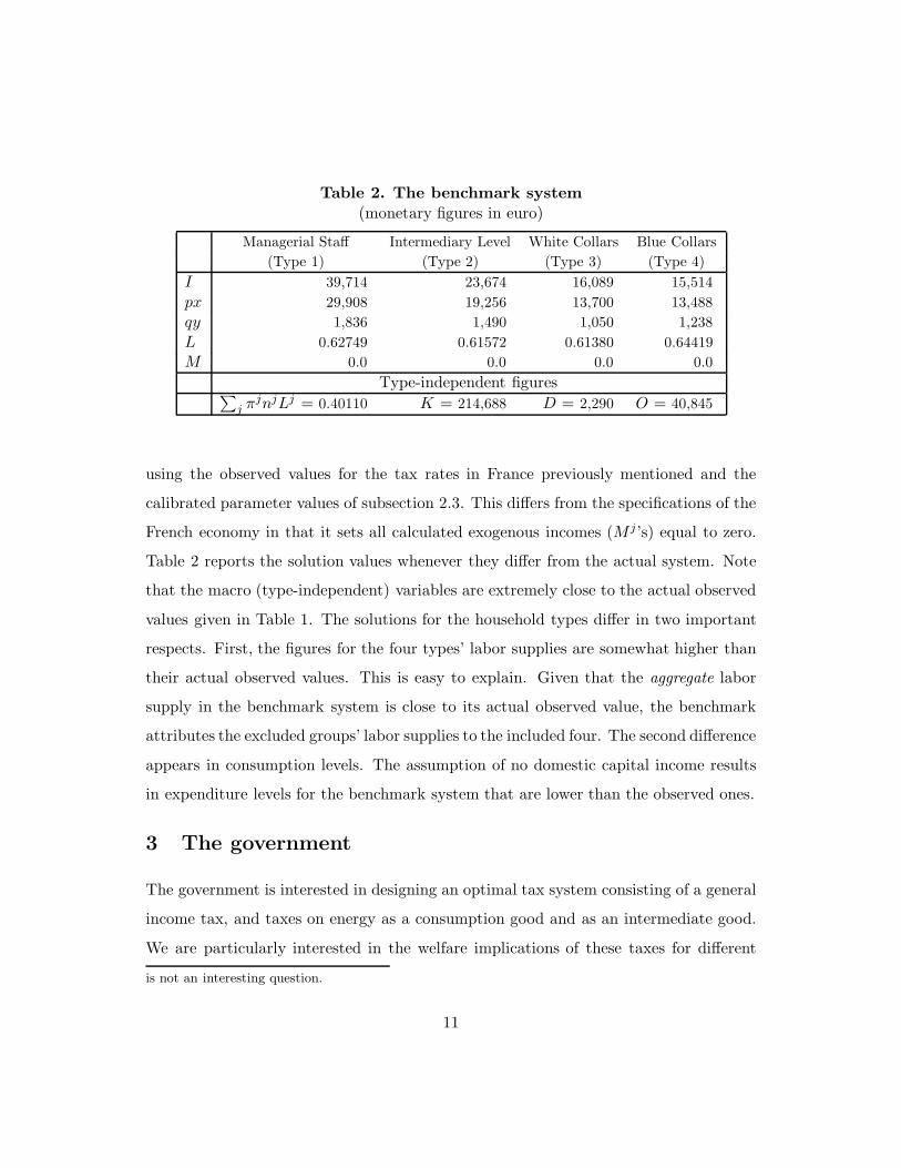
Table 2. The benchmark system(monetary figures in euro)

Managerial Staff Intermediary Level White Collars Blue Collars(Type 1) (Type 2) (Type 3) (Type 4)

I 39,714 23,674 16,089 15,514px 29,908 19,256 13,700 13,488qy 1,836 1,490 1,050 1,238L 0.62749 0.61572 0.61380 0.64419M 0.0 0.0 0.0 0.0

Type-independent figures∑j πjnjLj = 0.40110 K = 214,688 D = 2,290 O = 40,845

using the observed values for the tax rates in France previously mentioned and the

calibrated parameter values of subsection 2.3. This differs from the specifications of the

French economy in that it sets all calculated exogenous incomes (M j ’s) equal to zero.

Table 2 reports the solution values whenever they differ from the actual system. Note

that the macro (type-independent) variables are extremely close to the actual observed

values given in Table 1. The solutions for the household types differ in two important

respects. First, the figures for the four types’ labor supplies are somewhat higher than

their actual observed values. This is easy to explain. Given that the aggregate labor

supply in the benchmark system is close to its actual observed value, the benchmark

attributes the excluded groups’ labor supplies to the included four. The second difference

appears in consumption levels. The assumption of no domestic capital income results

in expenditure levels for the benchmark system that are lower than the observed ones.

3 The government

The government is interested in designing an optimal tax system consisting of a general

income tax, and taxes on energy as a consumption good and as an intermediate good.

We are particularly interested in the welfare implications of these taxes for different

is not an interesting question.

11

groups of households. With the energy taxes, we differentiate between two cases: Once

when commodity taxes must be taxed linearly and once when they can be levied at

different rates on different groups. Finally, we consider a situation where the tax ad-

ministration has the capability of observing the types and is thus able to levy differential

lump-sum taxes. This case shows the best that is hypothetically possible. It thus sets a

yardstick for judging the effectiveness of second-best taxes in attaining the government’s

efficiency and redistributive goals.

The design of an optimal tax structures must be based on some underlying social

welfare function. For this purpose, we will use an iso-elastic social welfare function of

the form

W =1

1 − η

4∑

j=1

πj(fj)1−η η 6= 1 and 0 ≤ η < ∞, (15)

where η is the “inequality aversion index”. The higher is η the more the society values

equality.14

In choosing a value for η (the inequality aversion index) for our optimal tax calcula-

tions, we will be guided by the observed degree of redistribution in the existing French

tax system. Bourguignon and Spadaro (2000) have recently studied France’s social pref-

erences as revealed through its tax system. They find that, if the uncompensated wage

elasticity of labor supply is 0.1, the marginal social welfare falls from 110 to 90 percent

of the mean as income increases from the lowest to the highest level. The fall would be

from 150 percent to 50 percent if the uncompensated labor elasticity is 0.5.

With the social welfare function (15), the marginal social utility of income for a

j-type person is given by∂fj

∂M j(fj)−η.

This implies that the ratio of the marginal social utility of the Managerial Staff’s14As is well-known, η = 0 implies a utilitarian social welfare function and η → ∞ a Rawlsian. When

η = 1, the social welfare function is given by W =∑4

j=1 πj ln(fj).

12

(type 1)income to Blue Collars’s (type 4) income is

∂f1/∂M1

∂f4/∂M4

(f4

f1

)η

.

Calculating the values for ∂fj/∂M j and fj (j = 1, 4) based on the French data sum-

marized in Table 1, setting the above expression equal to 9/11, we derive a value for

η equal to 0.1. This is the implied value for the inequality aversion index in France (if

the uncompensated wage elasticity of labor supply is 0.1). Similarly, setting the above

expression equal to 5/15, we derive a value for η equal to 1.9 for the implied value of

the inequality aversion index in France (if the uncompensated wage elasticity of labor

supply is 0.5).

3.1 Measuring welfare changes

A change in the government’s tax policy, environmental or otherwise, changes the welfare

different households differently. We shall measure these using the Hicksian “equivalent

variation” concept of a welfare change, EV . The changes are calculated relative to the

benchmark system. Denote a j-type’s indirect utility function by v(.; θj). Then, in

going from the benchmark to some other tax system (a different value for τD, p− 1, q−

1, tj , Gj, M j), we can calculate an EV ji (for each type j = 1, 2, 3, 4), from the following

relationship

v(pB, qB, wjn,B, Gj

B + M jB + EV j

i ; θj) − φ( 4∑

j=1

πjyjB + DB

)=

v(pi, qi, wjn,i, G

ji + M j

i ; θj) − φ( 4∑

j=1

πjyji + Di

),

where subscript B denotes the benchmark and subscript i refers to an alternative tax

option.15 We will then measure the “welfare change” in going from policy i to k for15The notation assumes individuals face the same prices for consumption goods. If they do not, prices

will also be indexed by j.

13

individual j by EV jk − EV j

i .16

Similarly, we can associate a measure of “aggregate welfare change” to any tax policy

by calculating how much one has to uniformly compensate each individual under the

benchmark system, to bring social welfare under the benchmark to parity with that

under the considered tax policy. Formally, the aggregate welfare measure associated

with going from the benchmark B to the alternative tax system i, EV Si , is found from

4∑

j=1

πj[v(pB, qB, w

jn,B, G

jB + M

jB + EV S

i ; θj) − φ( 4∑

j=1

πjyjB + DB

)]1−η=

4∑

j=1

πj[v(pi, qi, w

jn,i, G

ji + M j

i ; θj) − φ( 4∑

j=1

πjyji + Di

)]1−η.

4 The optimal general income tax with linear energy taxes

The standard assumption in the optimal income tax literature a la Mirrlees is that in-

comes are publicly observable so that the tax administration can levy an optimal general

income tax. We adopt this, and the accompanying, assumption on the unobservability

of wages and labor supplies in order to rule out differential lump-sum taxation. Regard-

ing consumption taxes, we shall assume that the available information is on anonymous

transactions (and not on personal consumption levels which would be difficult to justify).

This rules out nonlinear consumption taxes. In determining the mix of optimal general

income and linear consumption taxes, we follow Cremer and Gahvari (1997)’s method

and begin with the characterization of Pareto-efficient allocations that are constrained

not only by the standard self-selection constraints and the resource balance, but also by

the linearity of commodity taxes. However, the current problem is fundamentally more

complex than Cremer and Gahvari (1997)’s (as well as the traditional optimal income16This is of course different from calculating the EV in going “directly” from i to k. Whereas this latter

concept measures the “monetary equivalent” of the utility change in terms of prices in i, EV jk − EV j

i

is calculated in terms of pB (regardless of what k and i are). This way, one can compare the welfarechange in going from i to k versus, say, s to l, in a meaningful manner.

14

tax problems a la Mirrlees). The endogeneity of w adds another dimension to the prob-

lem which is generally missing in the formulation of optimal income tax problems.17

This requires us to extend Cremer and Gahvari’s method, as explained below.

We start by deriving an optimal revelation mechanism that consists of a set of type-

specific before-tax incomes, Ij ’s, aggregate expenditures on private goods, cj ’s, and a

fixed tax rate (same for everyone) on the polluting good, q − 1. Observe that, with

one extra degree in setting the commodity tax rates, due to demand and labor supply

functions being homogeneous of degree zero in prices and income, we have set the tax

rate on the nonpolluting goods equal to zero so that p = 1. This procedure determines

the polluting tax rate right from the outset. A complete solution to the optimal tax

problem per-se then requires only the design of a general income tax function.

The mechanism assigns (Ij, cj, q) to an individual who reports type j; the consumer

then allocates cj between the produced goods, x and y.18Denote Gj + wjnLj ≡ cj. One

can then determine, by setting M j = 0 in equations (11) and (12), the “conditional”

demand functions for xj and yj as xj = x(p, q, cj; θj) and yj = y(p, q, cj; θj). These

functions are independent of individual j’s labor supply because of the weak separability

of his preferences.19 Substituting these equations in the j-type’s utility function, we have

V

(p, q, cj,

Ij

wnj; θj

)≡ U

(x(p, q, cj; θj), y(p, q, cj; θj),

Ij

wnj; θj

).

The problem of the government is then to derive q, w and the second-best allocations

as the solution to

maxq,cj ,Ij ,K,D,w

11 − η

4∑

j=1

πj

V

(p, q, cj, Ij/wnj ; θj

)− φ

4∑

j=1

πjy(p, q, cj; θj

)− φD

1−η

(16)17Naito (1999) is an exception.18Strictly speaking, this procedure does not characterize “allocations” as such; the optimization is

over a mix of quantities and prices. However, given the commodity prices, utility maximizing individualswould choose the quantities themselves. We can thus think of the procedure as indirectly determiningthe final allocations.

19The functions, and the corresponding indirect utility function V (;θj), are conditional on cj; theydiffer from the customary Marshallian demand and indirect utility functions.

15

under the resource constraint,

O (L, K, D)−4∑

j=1

πj[x

(p, q, cj; θj

)+ y

(p, q, cj; θj

)]− rK − D − R ≥ 0, (17)

the incentive compatibility constraints,

V

(p, q, cj,

Ij

wnj; θj

)≥ V

(p, q, ck,

Ik

wnj; θj

)j 6= k = 1, 2, 3, 4, (18)

and the endogeneity of wage condition

w − OL (L, K, D) = 0, (19)

with

L =4∑

j=1

πjnjLj =4∑

j=1

πj Ij

w. (20)

The problem is solved analytically in the Appendix. It is interesting to note here an

implication of the production efficiency result. This is that condition w−OL (L, K, D) =

0 imposes no constraint on the problem (i.e., the Lagrangian multiplier associated with

it is zero while w = OL(.)). We prove this formally in the Appendix. The numerical

solutions are derived using GAUSS’s constrained optimization program.20 The first row

of Table 3 reports four values for the optimal tax on the polluting good based on two

values for the marginal social damage of emissions and two values for the inequality

aversion index. The second row reports the values for the optimal tax on the pollut-

ing input. Additionally, the third row reports the values for the so-called “Pigouvian

tax”. This is defined as the marginal social damage of pollution. It is measured by[∑j πj(fj)−η

]φ/µ, given our specification of the social welfare function and prefer-

ences.21

20This program, with a number of different iterative algorithms, is particularly suitable for opti-mization of nonlinear functions subject to nonlinear inequality constraints. One such routine, which wehave used, is the Boyden-Fletcher-Goldfarb-Shanno (BFGS) method known for its excellent convergenceproperties even for ill-behaved problems.

21This is Cremer et al.’s (1998) definition of the Pigouvian tax. Bovenberg and van der Ploeg (1994),Bovenberg and de Mooij (1994) and others use the Samuelson’s rule for optimal provision of publicgoods to define the “Pigouvian tax”. They term a tax Pigouvian if it is equal to the sum of the privatedollar costs of the environmental damage per unit of the polluting good across all households. In ournotation, their Pigouvian tax is

∑j πjφ/αj, where αj is the j-type’s private marginal utility of income.

16

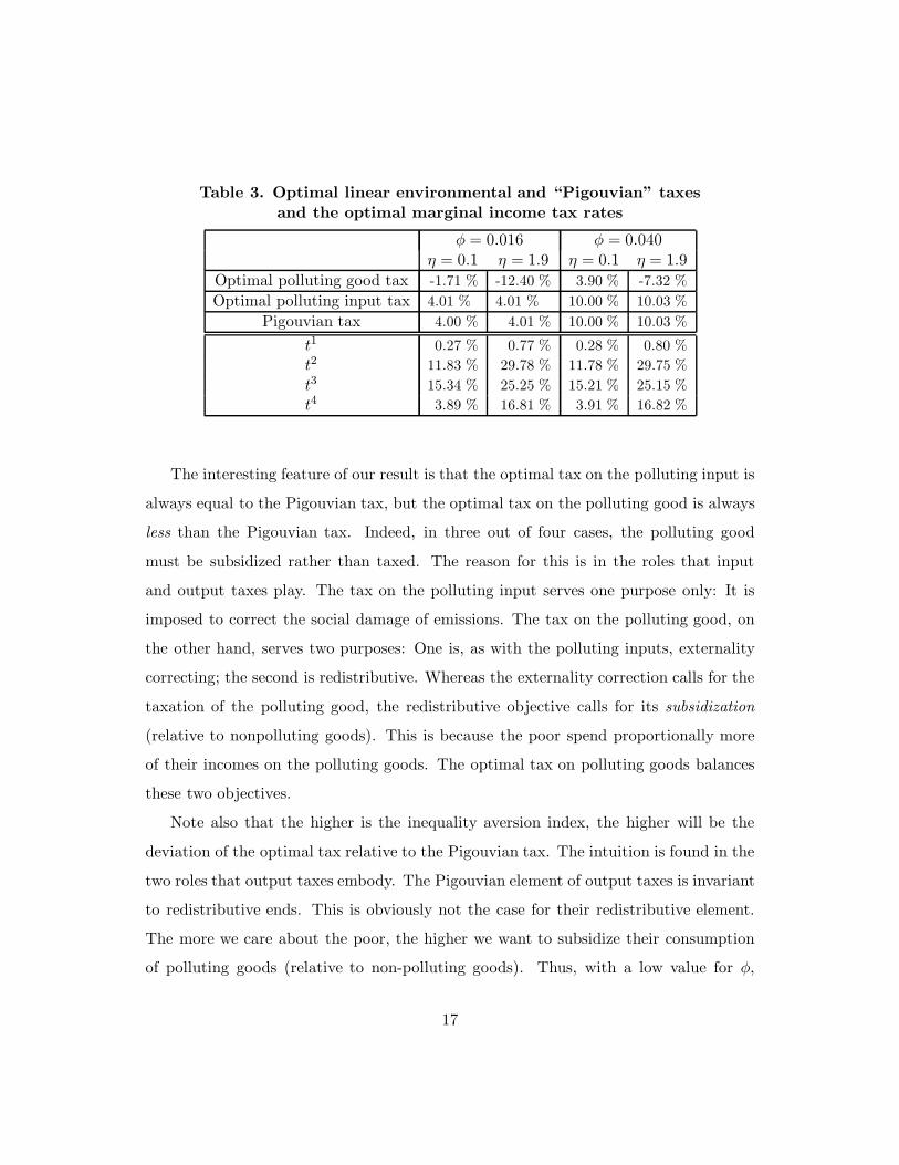
Table 3. Optimal linear environmental and “Pigouvian” taxesand the optimal marginal income tax rates

φ = 0.016 φ = 0.040η = 0.1 η = 1.9 η = 0.1 η = 1.9

Optimal polluting good tax -1.71 % -12.40 % 3.90 % -7.32 %Optimal polluting input tax 4.01 % 4.01 % 10.00 % 10.03 %

Pigouvian tax 4.00 % 4.01 % 10.00 % 10.03 %

t1 0.27 % 0.77 % 0.28 % 0.80 %t2 11.83 % 29.78 % 11.78 % 29.75 %t3 15.34 % 25.25 % 15.21 % 25.15 %t4 3.89 % 16.81 % 3.91 % 16.82 %

The interesting feature of our result is that the optimal tax on the polluting input is

always equal to the Pigouvian tax, but the optimal tax on the polluting good is always

less than the Pigouvian tax. Indeed, in three out of four cases, the polluting good

must be subsidized rather than taxed. The reason for this is in the roles that input

and output taxes play. The tax on the polluting input serves one purpose only: It is

imposed to correct the social damage of emissions. The tax on the polluting good, on

the other hand, serves two purposes: One is, as with the polluting inputs, externality

correcting; the second is redistributive. Whereas the externality correction calls for the

taxation of the polluting good, the redistributive objective calls for its subsidization

(relative to nonpolluting goods). This is because the poor spend proportionally more

of their incomes on the polluting goods. The optimal tax on polluting goods balances

these two objectives.

Note also that the higher is the inequality aversion index, the higher will be the

deviation of the optimal tax relative to the Pigouvian tax. The intuition is found in the

two roles that output taxes embody. The Pigouvian element of output taxes is invariant

to redistributive ends. This is obviously not the case for their redistributive element.

The more we care about the poor, the higher we want to subsidize their consumption

of polluting goods (relative to non-polluting goods). Thus, with a low value for φ,

17

Table 4. Emission and welfare changes in going to an optimalenvironmental-cum-general-income-tax system

(monetary figures in euro)

φ = 0.016 φ = 0.040η = 0.1 η = 1.9 η = 0.1 η = 1.9

E 5.48 % 3.34 % 2.93 % 0.82 %EV 1 -6,528 -8,068 -6,585 -8,120EV 2 -379 -547 -399 -566EV 3 2,458 2,715 2,469 2,725EV 4 2,066 2,405 2,072 2,409EV S 405 1,202 398 1,202

when η increases from 0.1 to 1.9, the optimal subsidy on energy consumption increases

from 1.71% to 12.40%; but the Pigouvian tax remains very much unchanged at 4%.

Similarly, with a high value for φ, when η increases from 0.1 to 1.9, the optimal tax

on the consumption decreases from 3.90% to an outright subsidy of 7.32%; with the

Pigouvian tax remaining unchanged at 10%.22

The last four rows in Table 3 report the marginal income tax rates on the four types.

These rates are radically different from the four marginal tax rates that are currently

in place in France (28.8% on type 1, 19.2% on Type 2, 14.4% on Type 3, and 9.6% on

Type 4). Note that in every case the highest ability persons face an extremely low, but

nevertheless a non-zero, marginal tax rate. That this rate is not strictly zero is due to

the linearity of commodity taxes imposed as an additional constraint on the second-

best; see Cremer et al. (1998). Note also that the marginal income tax rates increase

for all types as the inequality aversion index increases.

The first row in Table 4 reports the changes in aggregate emissions. It indicates

that the optimal policy entails an increase in aggregate emissions. This occurs for two22The alternative definition of the Pigouvian tax yields the following values for φ

∑j πj/αj : 3.88%

(φ = 0.016, η = 0.1), 3.68% (φ = 0.016, η = 1.9), 9.68% (φ = 0.40, η = 0.1), and 9.19% (φ = 0.040, η =1.9). Note that these values also exceed the values for the optimal polluting good taxes. However, theyare smaller than the optimal input taxes.

18

reasons. First, the optimal policy entails a cut in taxes on energy-related consumption

goods thus boosting their demand. Secondly, the increased efficiency of the tax system

as a whole encourages production and with it energy use and consumption. Note that

the introduction of taxes on energy inputs, on the other hand, has a dampening effect

on the use of energy and thus works to mitigate the increase in emissions.

On the redistributive front, the tax system becomes much more progressive. The

implied EV figures, and the associated social welfare changes, are reported in Table 4.

The magnitude of the changes are extremely large. When φ = 0.016 and η = 0.1, the

loss in Type 1’s welfare amounts to as much as 6,528 euro. Type 2 loses by 379 euro

and Types 3 and 4 gain by 2,458 and 2,066 euro. These translate into a social welfare

gain of 405 euro. Similar results hold when When φ = 0.040 and η = 0.1. Moreover, as

one might expect, the gains to the poor and the losses of the rich increase with η. The

increase in social welfare is also more pronounced for the higher value of η.

These changes come about as a result of the change in the whole structure of the tax

system, and particularly the change in the income tax structure. To isolate the effects of

environmental taxes per se, we also find the tax equilibrium of the economy while only

setting the income tax optimally keeping the energy taxes fixed at their current values.

Then compare the resulting equilibrium with the previously calculated optimal system.

Any difference must be due solely to the change in environmental taxes. The procedure

for the determination of the new equilibrium is the same as problem (16)–(20) above,

with some adjustments. This requires one to impose two additional constraints on the

problem. They are, given the current 40.32% average energy consumption tax relative

to other goods and zero energy input taxes,

q = 1.4032, (21)

OD (L, K, D) = 1. (22)

The first constraint implies that we no longer optimize with respect to q; the second

constraint enters as an additional term in the Lagrangian expression. The interesting

19

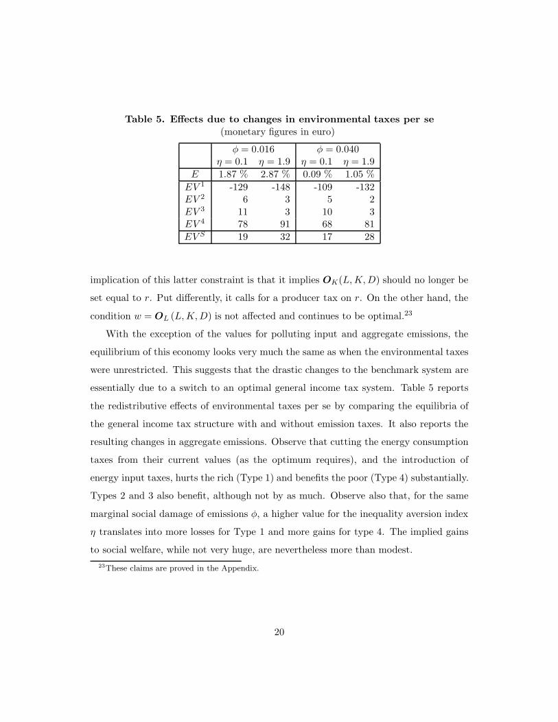
Table 5. Effects due to changes in environmental taxes per se(monetary figures in euro)

φ = 0.016 φ = 0.040η = 0.1 η = 1.9 η = 0.1 η = 1.9

E 1.87 % 2.87 % 0.09 % 1.05 %EV 1 -129 -148 -109 -132EV 2 6 3 5 2EV 3 11 3 10 3EV 4 78 91 68 81EV S 19 32 17 28

implication of this latter constraint is that it implies OK(L, K, D) should no longer be

set equal to r. Put differently, it calls for a producer tax on r. On the other hand, the

condition w = OL (L, K, D) is not affected and continues to be optimal.23

With the exception of the values for polluting input and aggregate emissions, the

equilibrium of this economy looks very much the same as when the environmental taxes

were unrestricted. This suggests that the drastic changes to the benchmark system are

essentially due to a switch to an optimal general income tax system. Table 5 reports

the redistributive effects of environmental taxes per se by comparing the equilibria of

the general income tax structure with and without emission taxes. It also reports the

resulting changes in aggregate emissions. Observe that cutting the energy consumption

taxes from their current values (as the optimum requires), and the introduction of

energy input taxes, hurts the rich (Type 1) and benefits the poor (Type 4) substantially.

Types 2 and 3 also benefit, although not by as much. Observe also that, for the same

marginal social damage of emissions φ, a higher value for the inequality aversion index

η translates into more losses for Type 1 and more gains for type 4. The implied gains

to social welfare, while not very huge, are nevertheless more than modest.23These claims are proved in the Appendix.

20

Table 6. The representative consumer(monetary figures in euro)

Data SummaryI = 16, 332 px = 24, 244 qy = 1, 890 M = 14, 329 L = 0.47879G = 3, 468 t = 18.51% n = 0.63992 a = 0.99999 b = 0.81206

BenchmarkI = 21, 328 px = 17, 431 qy = 1, 359 M = 0 L = 0.62525G = 1, 410 K = 214, 160 D = 2, 284 O = 40, 744

5 The one-consumer representation

Consider again the French economy described in Sections 2–3. A “one-consumer” repre-

sentation of this economy would average the four groups’ earning abilities, labor supplies,

incomes and expenditures and calculate a single tax bracket for them. These are shown

in the first two rows of Table 6. (The rest of the variables take identical values to those

given in table 1). Next, as in Subsection 2.4, this representation is simplified so that it

satisfies the assumptions of our model. We thus should have all households working and

that all capital is imported. Rows 3–4 in Table 6 report the solution values whenever

they differ from the actual data.

As in Section 2, the consumer maximizes his utility function represented by (7)–(9)

subject to his budget constraint (11)—all specified for one type. Then equations (11)–

(13) determine his demand functions for good and his labor supply, and consequently

indirect utility, as functions of p, q, wn and G. The government’s problem can then be

specified as one of choosing its tax instruments, q − 1, t (the income tax rate), an input

tax on D [equal to OD(L, K, D)−1], and an input tax on K [equal to OK(L, K, D)−r],

in order to maximize24

v(p, q, wn, G)− φ [y(p, q, wn, G) + D] , (23)24Again, the tax rate on x is normalized at one, so that p = 1.

21

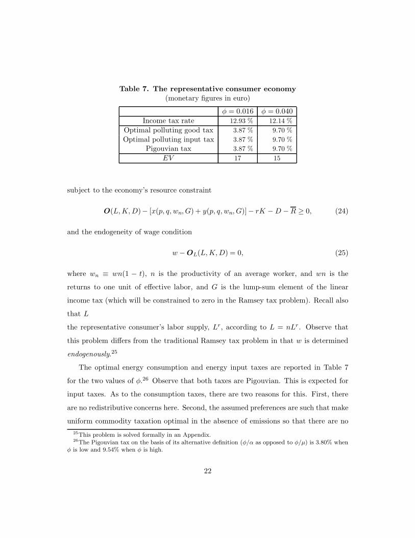
Table 7. The representative consumer economy(monetary figures in euro)

φ = 0.016 φ = 0.040Income tax rate 12.93 % 12.14 %

Optimal polluting good tax 3.87 % 9.70 %Optimal polluting input tax 3.87 % 9.70 %

Pigouvian tax 3.87 % 9.70 %EV 17 15

subject to the economy’s resource constraint

O(L, K, D)− [x(p, q, wn, G) + y(p, q, wn, G)]− rK − D − R ≥ 0, (24)

and the endogeneity of wage condition

w − OL(L, K, D) = 0, (25)

where wn ≡ wn(1 − t), n is the productivity of an average worker, and wn is the

returns to one unit of effective labor, and G is the lump-sum element of the linear

income tax (which will be constrained to zero in the Ramsey tax problem). Recall also

that L denotes aggregate effective labor [as defined by equation (14)] and differs from

the representative consumer’s labor supply, Lr, according to L = nLr . Observe that

this problem differs from the traditional Ramsey tax problem in that w is determined

endogenously.25

The optimal energy consumption and energy input taxes are reported in Table 7

for the two values of φ.26 Observe that both taxes are Pigouvian. This is expected for

input taxes. As to the consumption taxes, there are two reasons for this. First, there

are no redistributive concerns here. Second, the assumed preferences are such that make

uniform commodity taxation optimal in the absence of emissions so that there are no25This problem is solved formally in an Appendix.26The Pigouvian tax on the basis of its alternative definition (φ/α as opposed to φ/µ) is 3.80% when

φ is low and 9.54% when φ is high.

22

efficiency reasons for Ramsey taxes either. This is very much at odds with the result

derived for the heterogeneous individuals case where the tax rate reflects redistributional

concerns.27

To isolate the welfare effects of environmental taxes per se, we also find the tax

equilibrium of the economy under the constraints q = 1.4032 and OD(L, K, D) = 1,

optimizing over the income tax t and the tax on K only.28 The results are also presented

in Table 7. They are much smaller than the corresponding social welfare changes in

the heterogeneous individuals case. Most importantly, by nature, they cannot tell us

anything about how differently the poor and the rich will be affected by these taxes.

6 Summary and conclusion

This paper has explored the design of an optimal general income tax system when earn-

ing abilities are endogenous, and when energy is used both as a polluting consumption

good and a polluting input. It has shown that the optimal marginal income tax rates

are radically different from the rates that are currently in place in France. The existing

rates of 28.8% on type 1, 19.2% on Type 2, 14.4% on Type 3, and 9.6% on Type 4

are replaced by approximately 0.3%, 111.8%, 15.3% and 3.9% if the inequality aversion

index is 0.1, and by 0.8%, 29.8%, 25.2% and 16.8% if the inequality aversion index is

1.9. In both cases, the tax system becomes far more redistributive towards the poor

and more efficient. The gains and losses run in thousands of euro per household. So-

cial welfare also increases markedly by about 400 euro per household if the inequality

aversion index is 0.1 and just over 1,200 euro when the index is 1.9.27Strictly speaking, the change in energy consumption taxes in our model reflects the types’ different

preferences. Given weak separability of labor, and a general income tax, commodity taxes are redundantunless to correct for externalities if all households have the same preferences; see Cremer et al. (1998).Our varying preferences should be considered as local approximations to a more general and nonseparablepreferences.

28The restriction that the tax rate on the polluting inputs must be zero implies that at the optimumthere should be a tax on K. That is, there will be a wedge between r and the marginal product of K.In the absence of this restriction, there will be no such wedge.

23

In the case of environmental taxes, the paper has shown that the optimal tax on

energy inputs is Pigouvian and equal to its marginal social damage. The optimal tax on

the consumption of energy, on the other hand, is less than its marginal social damage.

In fact, in three out of four cases, energy consumption should be subsidized. This is in

marked contrast to the current tax system in France which taxes energy consumption

over 40% relative to non-energy related goods. The reason for this is the fact that the

poor spend proportionally more of their income on energy consumption than the rich.

To gauge the welfare implications of environmental taxes per se, we have compared

the optimal general income tax equilibria at the current environmental taxes and at

their optimal values. The results indicated substantial losses for the rich (Type 1) and

substantial gains for the poor (type 4). In comparison, the effects on Types 2 and 3

were rather marginal.

Finally, we compared our findings with those that result if one models the economy

in terms of a representative household. The comparison shows that a most significant

aspect of energy consumption taxes is missed in a one-consumer representation of the

economy. The redistributive aspects of such taxes, while quite important, are naturally

masked in such an analysis. Moreover, this may lead the government to levy taxes on

energy while in fact a subsidy is required. This is just one indication of why we believe

that in calculating optimal income and consumption taxes, including environmental

taxes, one should go beyond the traditional Ramsey tax framework. The methods of this

paper can be used to compute optimal tax structures for other countries. Better data

may allow for a greater number of types. It should also allow for a more disaggregated

set of goods and better parameter estimates. Another extension would be to consider

non-homothetic preferences directly. The current paper should be viewed more for its

methodological contribution to this endeavor, rather than the exactness of the reported

numbers. Nevertheless the numbers are very interesting even if only indicative.

24

Appendix

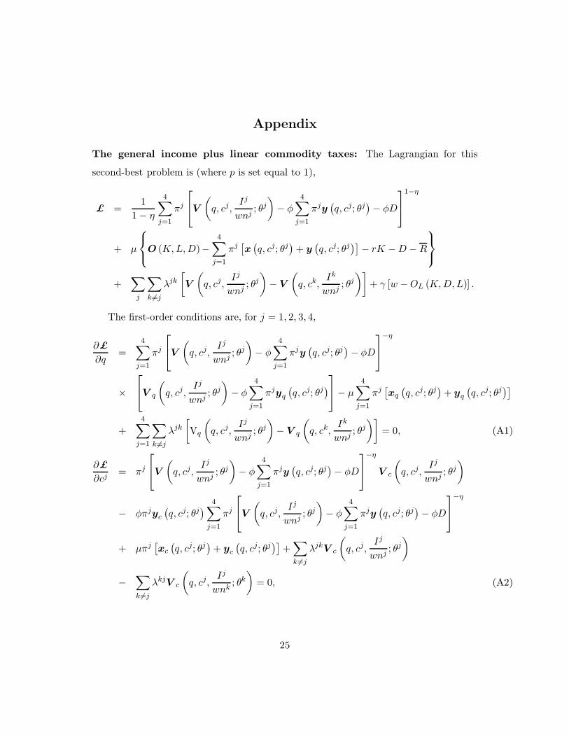
The general income plus linear commodity taxes: The Lagrangian for this

second-best problem is (where p is set equal to 1),

£ =1

1 − η

4∑

j=1

πj

V

(q, cj,

Ij

wnj; θj

)− φ

4∑

j=1

πjy(q, cj; θj

)− φD

1−η

+ µ

O (K, L, D)−

4∑

j=1

πj[x

(q, cj; θj

)+ y

(q, cj; θj

)]− rK − D − R

+∑

j

∑

k 6=j

λjk

[V

(q, cj,

Ij

wnj; θj

)− V

(q, ck,

Ik

wnj; θj

)]+ γ [w − OL (K, D, L)] .

The first-order conditions are, for j = 1, 2, 3, 4,

∂£

∂q=

4∑

j=1

πj

V

(q, cj,

Ij

wnj; θj

)− φ

4∑

j=1

πjy(q, cj; θj

)− φD

−η

×

V q

(q, cj,

Ij

wnj; θj

)− φ

4∑

j=1

πjyq

(q, cj; θj

) − µ

4∑

j=1

πj[xq

(q, cj; θj

)+ yq

(q, cj; θj

)]

+4∑

j=1

∑

k 6=j

λjk

[Vq

(q, cj,

Ij

wnj; θj

)− V q

(q, ck,

Ik

wnj; θj

)]= 0, (A1)

∂£

∂cj= πj

V

(q, cj,

Ij

wnj; θj

)− φ

4∑

j=1

πjy(q, cj; θj

)− φD

−η

V c

(q, cj,

Ij

wnj; θj

)

− φπjyc

(q, cj; θj

) 4∑

j=1

πj

V

(q, cj,

Ij

wnj; θj

)− φ

4∑

j=1

πjy(q, cj; θj

)− φD

−η

+ µπj[xc

(q, cj; θj

)+ yc

(q, cj; θj

)]+

∑

k 6=j

λjkV c

(q, cj,

Ij

wnj; θj

)

−∑

k 6=j

λkjV c

(q, cj,

Ij

wnk; θk

)= 0, (A2)

25

∂£

∂Ij= πj

V

(q, cj ,

Ij

wnj; θj

)− φ

4∑

j=1

πjy(q, cj; θj

)− φD

−η

1wnj

V L

(q, cj,

Ij

wnj; θj

)

+ µOL(L, K, D)πj

w+

∑

k 6=j

λjk 1wnj

V L

(q, cj,

Ij

wnj; θj

)

−∑

k 6=j

λkj 1wnk

V L

(q, cj ,

Ij

wnk; θk

)− γ

πj

wOLL(L, K, D) = 0, (A3)

∂£

∂D= −

4∑

j=1

πj

V

(q, cj,

Ij

wnj; θj

)− φ

4∑

j=1

πjy(q, cj; θj

)− φD

−η

φ

+ µ (OD(L, K, D)− 1)− γOLD(L, K, D) = 0, (A4)∂£

∂K= µ (OK(L, K, D)− r) − γOLK(L, K, D) = 0, (A5)

∂£

∂w=

4∑

j=1

πj

V

(q, cj,

Ij

wnj; θj

)− φ

4∑

j=1

πjy(q, cj; θj

)− φD

−η (

−Ij

njw2

)V L

(q, cj,

Ij

wnj; θj

)

+ µOL(L, K, D)−1w2

4∑

j=1

πjIj +4∑

j=1

∑

k 6=j

λjk

(−Ij

njw2

)VL

(q, cj,

Ij

wnj; θj

)

+4∑

j=1

∑

k 6=j

λjk

(Ik

njw2

)V L

(q, ck,

Ik

wnj; θj

)+ γ

1 +

1w2

4∑

j=1

πjIjOLL(L, K, D)

= 0. (A6)

Next, note that production efficiency implies that the condition w = OL(L, K, D)

imposes no constraint on the problem so that γ = 0 (we show this below). This simplifies

equations (A3)–(A6) into

∂£

∂Ij= πj

V

(q, cj,

Ij

wnj; θj

)− φ

4∑

j=1

πjy(q, cj; θj

)− φD

−η

1wnj

V L

(q, cj,

Ij

wnj; θj

)+ µπj

+∑

k 6=j

λjk 1wnj

V L

(q, cj,

Ij

wnj; θj

)−

∑

k 6=j

λkj 1wnk

V L

(q, cj,

Ij

wnk; θk

)= 0, (A7)

∂£

∂D= −

4∑

j=1

πj

V

(q, cj,

Ij

wnj; θj

)− φ

4∑

j=1

πjy(q, cj; θj

)− φD

−η

φ

+ µ (OD(L, K, D)− 1) = 0, (A8)

26

∂£

∂K= µ (OK(L, K, D)− r) = 0, (A9)

∂£

∂w= −

4∑

j=1

(Ij

w)∂£

∂Ij= 0. (A10)

Proof of γ = 0: Multiply equation (A3) through by Ij/w, sum over j and simplify to

get

− 1w2

4∑

j=1

πjIj

nj

V

(q, cj,

Ij

wnj; θj

)− φ

4∑

j=1

πjy(q, cj; θj

)− φD

−η

V L

(q, cj,

Ij

wnj; θj

)

= µL +1w2

∑

j

∑

k 6=j

[(Ij

nj)λjkV L

(q, cj,

Ij

wnj; θj

)− (

Ij

nk)λkjV L

(q, cj,

Ij

wnk; θk

)]

− 1w2

γOLL(L, K, D)(wL). (A11)

Substituting (A11) into (A6) and simplifying, one gets

∑

j

∑

k 6=j

(Ij

nk)λkjV L

(q, cj,

Ij

wnk; θk

)=

∑

j

∑

k 6=j

(Ik

nj)λjkV L

(q, ck,

Ik

wnj; θj

)+ γw2.

(A12)

But one can rewrite the left-hand side of (A12) as

∑

j

∑

k 6=j

(Ij

nk)λkjV L

(q, cj,

Ij

wnk; θk

)=

∑

j

∑

k 6=j

(Ik

nj)λjkV L

(q, ck,

Ik

wnj; θj

). (A13)

Substituting from (A13) into (A12) then implies

γ = 0.

The General income tax problem when q = 1.4032 and OD(L, K, D) = 1: The

implications of these constraints for the optimization problem of the government are

twofold. First, we no longer optimize with respect to q. Consequently, the first-order

conditions do not include equation (A1). Second, denote the Lagrange multiplier asso-

ciated with the constraint 1 − OD(L, K, D) = 0 by ζ. This brings about the following

27

changes in the first-order conditions (A2)–(A6): The expression for ∂£/∂cj remain un-

affected; the expression for ∂£/∂Ij now includes an additional term −ζODL(πj/w);

the expression for ∂£/∂D now includes an additional term −ζODD; the expression for

∂£/∂K now includes an additional term −ζODK ; and the expression for ∂£/∂w now

includes an additional term −ζODL(∑

πjIj/w2).

Using the same method as previously, one can again show that the Lagrange multi-

plier associated with the constraint OL(L, K, D) = w continues to be zero so that this

condition imposes no restriction on the problem even in the presence of the additional

constraint on OD(L, K, D). On the other hand, setting OD(L, K, D) = 1 in (A4)–(A5),

these will change to

−4∑

j=1

πj

[V

(q, cj,

Ij

wnj; θj

)− φ

4∑

j=1

πjy(q, cj; θj

)− φD ]−η φ

− ζODD(L, K, D) = 0, (A14)

µ (OK(L, K, D)− r) − ζODK(L, K, D) = 0. (A15)

Conditions (A14)–(A15) then imply that

OK(L, K, D) = r − ODK(L, K, D)µODD(L, K, D)

×

4∑

j=1

πj

V

(q, cj,

Ij

wnj; θj

)− φ

4∑

j=1

πjy(q, cj; θj

)− φD

−η

φ. (A16)

Thus, the constraint OD(L, K, D) = 1 implies that OK(L, K, D) should no longer be

set equal to r. Put differently, a producer tax on r is now optimal.

The Ramsey tax problem with endogenous w: The Lagrangian for this problem

is, where G is set equal to 0 and p equal to 1,

£ = v(p, q, wn, G)− φ [y(p, q, wn, G) + D] + γ [w − OL (K, D, L)]

+ µ[O (K, L, D)− x(p, q, wn, G)− y(p, q, wn, G)− rK − D − R

].

28

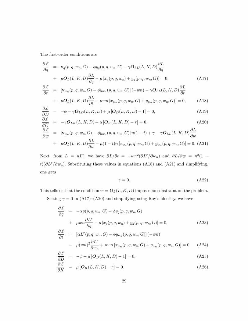
The first-order conditions are

∂£∂q

= vq(p, q, wn, G)− φyq(p, q, wn, G)− γOLL(L, K, D)∂L

∂q

+ µOL(L, K, D)∂L

∂q− µ [xq(p, q, wn) + yq(p, q, wn, G)] = 0, (A17)

∂£∂t

= [vwn(p, q, wn, G)− φywn(p, q, wn, G)] (−wn) − γOLL(L, K, D)∂L

∂t

+ µOL(L, K, D)∂L

∂t+ µwn [xwn(p, q, wn, G) + ywn(p, q, wn, G)] = 0, (A18)

∂£∂D

= −φ − γOLD(L, K, D)+ µ [OD(L, K, D)− 1] = 0, (A19)

∂£∂K

= −γOLK(L, K, D)+ µ [OK(L, K, D)− r] = 0, (A20)

∂£∂w

= [vwn(p, q, wn, G)− φywn(p, q, wn, G)]n(1 − t) + γ − γOLL(L, K, D)∂L

∂w

+ µOL(L, K, D)∂L

∂w− µ(1− t)n [xwn(p, q, wn, G) + ywn(p, q, wn, G)] = 0. (A21)

Next, from L = nLr, we have ∂L/∂t = −wn2(∂Lr/∂wn) and ∂L/∂w = n2(1 −

t)(∂Lr/∂wn). Substituting these values in equations (A18) and (A21) and simplifying,

one gets

γ = 0. (A22)

This tells us that the condition w = OL(L, K, D) imposes no constraint on the problem.

Setting γ = 0 in (A17)–(A20) and simplifying using Roy’s identity, we have

∂£∂q

= −αy(p, q, wn, G)− φyq(p, q, wn, G)

+ µwn∂Lr

∂q− µ [xq(p, q, wn) + yq(p, q, wn, G)] = 0, (A23)

∂£∂t

= [αLr(p, q, wn, G)− φywn(p, q, wn, G)] (−wn)

− µ(wn)2∂Lr

∂wn+ µwn [xwn(p, q, wn, G) + ywn(p, q, wn, G)] = 0, (A24)

∂£∂D

= −φ + µ [OD(L, K, D)− 1] = 0, (A25)

∂£∂K

= µ [OK(L, K, D)− r] = 0. (A26)

29

These equations determine the optimal Ramsey taxes in our setting.

Finally, to see the relationship with the standard Ramsey results, observe that equa-

tion (A26) implies OK(L, K, D)−r = 0, so that K should not be taxed. Similarly, equa-

tion (A25) yields OD(L, K, D)− 1 = φ/µ, and energy input should be taxed only for

Pigouvian considerations. Turning to the wage and energy consumption taxes, equa-

tions (A23)–(A24) can be simplified as follows. Differentiate the individual’s budget

constraint x + qy = wnLr once with respect to q and once with respect to wn. This

yields

∂x

∂q+

∂y

∂q= −y − (q − 1)

∂y

∂q+ wn

∂Lr

∂q,

∂x

∂wn+

∂y

∂wn= L + wn

∂Lr

∂wn− (q − 1)

∂y

∂wn.

Then substitute these values in equations (A23)–(A24) and simplify to arrive at(

1 − α

µ

)y +

(q − 1 − φ

µ

)∂y

∂q+ t(nw)

∂Lr

∂q= 0, (A27)

(1 − α

µ

)(−Lr) +

(q − 1 − φ

µ

)∂y

∂wn+ t(nw)

∂Lr

∂wn= 0. (A28)

Equations (A27)–(A28) are the standard equations derived in the Ramsey tax problem

when w is exogenous; see, for example, Cremer et al. (2001). The optimal tax on y will

then also be Pigouvian so that q − 1 = φ/µ.

The Ramsey tax problem when q = 1.4032 and OD(L, K, D) = 1: The implica-

tions of these constraints for the optimization problem of the government are twofold.

First, we no longer optimize with respect to q. Consequently, the first-order conditions

do not include equation (A17). Second, denote the Lagrange multiplier associated with

the constraint 1 − OD(L, K, D) = 0 by ζ. This brings about the following changes

in the first-order conditions (A18)–(A21): The expression for ∂£/∂t includes an addi-

tional term −ζODL(−wn2)(∂Lr/∂wn); the expression for ∂£/∂D includes an additional

term −ζODD; the expression for ∂£/∂K includes an additional term −ζODK ; and the

expression for ∂£/∂w includes an additional term −ζODLn2(1 − t)(∂Lr/∂wn).

30

Using the same method as previously, one can again show that the Lagrange mul-

tiplier associated with the constraint OL(L, K, D) = w continues to be zero (γ = 0)

so that this condition imposes no constraint on the problem even in the presence of

the additional constraint on OD(L, K, D). Now setting OD(L, K, D) = 1 and γ = 0 in

(A19)–(A20), these will change to

−φ − ζODD(L, K, D) = 0, (A29)

µ [OK(L, K, D)− r] − ζODK(L, K, D) = 0. (A30)

Conditions (A29)–(A30) then imply that

OK(L, K, D) = r − ODK(L, K, D)ODD(L, K, D)

φ

µ. (A31)

Thus, the constraint OD(L, K, D) = 1 implies that OK(L, K, D) should no longer be

set equal to r. Put differently, a producer tax on r is now optimal.

31

References

Berndt, E. R. and D. O. Wood (1975) “Technology, prices, and the derived demand forenergy,” Review of Economics and Statistics, 57, 259–268.

Berndt, E. R. and D. O. Wood (1985) Energy Price Shocks and Productivity Growthin US Manufacturing. Cambridge, MA: MIT Press.

Bourguignon, F. (1999) “Redistribution and labor-supply incentives,” mimeo.

Bourguignon, F. and A. Spadaro (2000) “Social preferences revealed through effectivemarginal tax rates,” mimeo.

Bovenberg, A.L. and F. van der Ploeg (1994) “Environmental policy, public finance andthe labor market in a second-best world,” Journal of Public Economics, 55, 349–390.

Bovenberg, A.L. and R.A. de Mooij (1994) “Environmental Levies and DistortionaryTaxation,” American Economic Review, 84, 1085–1089.

Bovenberg, A.L. and L. Goulder (1996) “Optimal environmental taxation in the pres-ence of other taxes: general equilibrium analyses,” American Economic Review, 86,985–1000.

Bovenberg, A.L. and L. Goulder (2002) “Environmental taxation and regulation,” inHandbook of Public Economics, Vol 3, ed. Auerbach, A. and M. Feldstein. Amster-dam: North-Holland, Elsevier, 1471–1545.

Cremer, H., Gahvari, F. and N. Ladoux (1998) “Externalities and optimal taxation,”Journal of Public Economics, 70, 343–364.

Cremer, H., Gahvari, F. and N. Ladoux (2003) “Environmental taxes with heterogeneousconsumers: an application to energy consumption in France,” Journal of Public

Economics, 87, 2791-2815.

Devezeaux de Lavergne J.G., Ivaldi M. and N. Ladoux (1990) “La forme flexible deFourier: une evaluation sur donnees macroeconomiques,” Annales dEconomie et de

Statistique, 17, .

(1997) “Les couts de reference de la production delectricite,” DGEMP-DIGEC, Min-istere de lEconomie et des Finances, , .

Gahvari, F. (2002) “Review of Ruud A. de Mooij: Environmental Taxation and theDouble Dividend,” Journal of Economic Literature, 40, 221–223.

Goulder, L.H., Parry, I.W.H., Williams III, R.C. and D. Burtraw (1999) “The costeffectiveness of alternative instruments for environmental protection in a second-bestsetting,” Journal of Public Economics, 72, 329–360.

Griffin, J.M. and P.R. Gregory (1976) “An intercountry translog model of energy sub-stitution responses,” American Economic Review, 66, 845–857.

32

INSEE (1998) “Comptes et Indicateurs Economiques, Rapport sur les Comptes de laNation 1997,” Serie INSEE Resultats, 165–167, ISBN 2-11-0667748-6.

INSEE (1989) “Emplois-revenus: enquete sur l’emploi de 1989, resultats detailles,” SerieINSEE Resultats, 28–29, ISBN 2-11-065325-6.

INSEE (1991a) “Consommation modes de vie: le budget des menages en 1989,” SerieConsommation Modes de Vie, 116–117, ISBN 2-11-065922-X.

INSEE (1991b) “Emplois-revenus: les salaires dans l’industrie, le commerce et les ser-vices en 1987–1989,” Serie INSEE Resultats, 367–369, ISBN 2-11-06-244-1.

INSEE (1998) “Comptes et indicateurs economiques: rapport sur les comptes de lanation 1997,” Serie INSEE Resultats, 165–167, ISBN 2-11-0667748-6.

Mayeres, I. and S. Proost (2001) “Marginal tax reform, externalities and income distri-bution,” Journal of Public Economics, 79, 343–363.

Ministere de l’Economie et des Finances (1989) “Publication N 2041 S,” France.

Naito, H. (1999) “Re-examination of uniform commodity taxes under a non-linear in-come tax system and its implication for production efficiency,” Journal of PublicEconomics, 71, 165–188.

Poterba, J.M. (1991) “Tax policy to combat global warming: on designing a carbontax,” in Global Warming: Economic Policy Responses, ed. Dornbusch, R. and J.M.Poterba. Cambridge, Massachusetts: The MIT Press.

Schob, R. (2003) “The double dividend hypothesis of environmental taxes: a survey,”CESifo Working Paper No. 946.

U.S. Environmental Protection Agency) (1998) “Marginal damage estimates for air pol-lutants,” http://www.epa.gov/oppt/epp/guidance/top20faqexterchart.htm.

33