Environmental Impacts of Cement Production - MDPI

applied sciences

Article

Environmental Impacts of Cement Production:A Statistical Analysis

Claudio Durastanti 1 and Laura Moretti 2,*1 Department of Basic and Applied Sciences for Engineering, Sapienza University of Rome, Via Antonio

Scarpa 16, 00161 Rome, Italy; [email protected] Department of Civil, Constructional and Environmental Engineering, Sapienza University of Rome,

Via Eudossiana 18, 00184 Rome, Italy* Correspondence: [email protected]; Tel.: +39-06-44-58-51-14

Received: 6 November 2020; Accepted: 17 November 2020; Published: 19 November 2020 �����������������

Abstract: The attention to environmental impacts of cement production has grown fast in recentdecades. The cement industry is a significant greenhouse gases emitter mainly due to the calcinationsof raw materials and the combustions of fuels. This paper investigates on the environmentalperformances of cement production and on the identification of factors driving emissions. For thispurpose, a sample of 193 different recipes of gray cement produced in Italy from 2014 to 2019 accordingto the European standard EN 197-1. This paper identifies the consumption impact categories (e.g.,fossil fuels, renewable and non-renewable secondary fuels) that explain the assessment of the GlobalWarming Potential, one of the most crucial impacts of cement production. Having regard to the overallexamined dataset and each cement type, a set of predictive models is implemented and evaluated.A similar approach has been adopted to produce accurate predictive models for further environmentalimpact categories that quantify emissions to air. The obtained results provide important informationthat can support cement producers to develop low-impacting cement recipes.

Keywords: life cycle analysis; cement production; EN 15804; regression analysis; AIC criterion

1. Introduction

In recent years, the interest for environmental protection has grown faster, becoming an importantcriterion for public policy in social and political contexts [1,2]. The most pursued objective is toreduce emissions of greenhouse gases (e.g., carbon dioxide, nitrous oxide and methane), which areresponsible for the greenhouse effect [3]. In particular, the cement industry contributes about 5%of global anthropogenic CO2 emissions excluding land-use change [4,5], as the production of thebinder is a highly energy-intensive and emitting process. Calcination of raw materials for the cementproduction (e.g., limestone, clay, calcareous marl and other clay-like materials) and burning (fossil)fuels to maintain high temperature in the kiln are the processes with highest environmental impact.The former is a chemical emission, the latter a physical emission. Indeed, raw materials are heatedinside large rotating furnaces at 1400 ◦C to form a solid substance called clinker [6]. During this process,chemical emissions mainly come from calcium carbonate (CaCO3) and magnesium carbonate (MgCO3)calcination according to Equations (1) and (2) [7,8]:

CaCO3(s) + heat→ CaO(s) + CO2 (g) (1)

MgCO3(s) + heat→MgO(s) + CO2 (g) (2)

Clinker is then ground or milled with gypsum and other constituents (e.g., products, raw materials,additives, recycled waste) to produce cement [9]. According to [9], 5 main types of cement (CEM I to

Appl. Sci. 2020, 10, 8212; doi:10.3390/app10228212 www.mdpi.com/journal/applsci

Appl. Sci. 2020, 10, 8212 2 of 25

CEM V) and 27 products in the family of common cements are defined. They differ for composition(proportion by mass) of the main constituents, but all contain clinker. Therefore, its productionaffects the environmental performances of the final product and cannot be overlooked in this study.The chemical process described in Equations (1) and (2) implies more than 60% of total CO2 emissionsdue to clinker production, as confirmed by the mass balance published in the last EnvironmentalProduct Declaration (EPD) of the Italian cement production [10]. Chemical emissions are not reducible,but physical emissions resulting from fuel combustion for kiln firing can be managed and reducedusing alternative/waste fuels [11] and/or by adopting energy-saving technologies [12]. However,these changes in production processes have to turn out in agreement with the required quality of theobtained products, related to construction or industrial uses [13], or with some special performancesto obtain [14–16]. Moreover, in order to reduce the impacts of cement production, in the last decadethe content of clinker in cement has decreased [17] using supplementary cementitious materials (e.g.,gypsum, ground limestone, coal fly ash or blast furnace slag) [18–20]. Therefore, the cement industryis making efforts to reduce its environmental impacts in terms of greenhouse gases that reflect onother environmental performances. The standard EN 15804 “Sustainability of construction works,environmental product declarations, core rules for the product category of construction products” [21]defines the core rules for the product category of construction Products in order to assess the life cycleimpact and develop a Type III environmental declaration (i.e., EPD) for any construction product andconstruction service [22].

According to [21], different parameters describe the environmental performances of a product,such as environmental impacts, resource use, waste categories, and output flows [23–27]. In theliterature, several studies assessed the impacts of cement production considering its upstream processes(i.e., production of commodities, raw materials, transport to the factory plant, production process) [28].The obtained results allow the cement industry to identify the best strategies to reduce its environmentalimpact. More in detail, the authors have Life Cycle Analysis (LCA) results of the Italian cementproduction from 2014 to 2019; this data refers to the environmental performances of one of the mostimportant cement industries in Europe with over 19 million of Mg produced in 2019 [29]. The impactsof more than 190 cement powders produced according to [9] have been assessed with a “from cradle togate” boundary approach using the database Ecoinvent 2.2 (Version 2.2, Ecoinvent, Zurich, Switzerland,2007) and the software package SimaPro 8.0.5.13 (Version 8.0.5.13, Pré Consultants: Amersfoort,The Netherlands, 2016) [30]. 15 different impact categories were assessed to describe the characteristicsof each cement powder recipe.

The goal of this work is to identify among these features the most relevant variables to predictthe behavior of Global Warming Potential (GWP). To obtain these results, different models have beenimplemented, by means of linear regression and variable selection procedures, more specifically,the Akaike Information Criterion. Analogous models are developed also for the other impact categoriesthat quantify emissions to air. A comparative analysis shows that the most important impact categoryto control GWP and other emissions is represented by the Abiotic depletion-fossil fuels (ADPf).

2. Data and Methods

After a quick introduction of the available dataset, this section provides the reader with the keyconcepts to investigate the behavior of the Global Warming Potential (GWP) and its connections withthe production parameters, as well as a short summary of the statistical methods here employed.

The examined impact categories (ICs) comply with the standard EN 15804 [21]; Table 1 lists theirname and units of measure.

Appl. Sci. 2020, 10, 8212 3 of 25

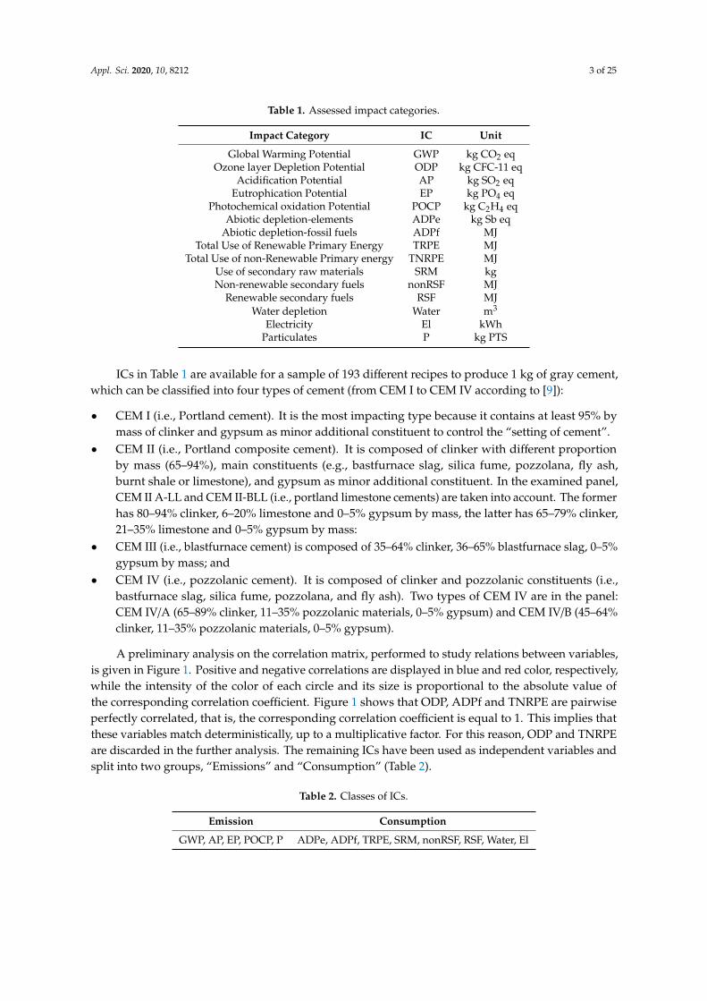
Table 1. Assessed impact categories.

Impact Category IC Unit

Global Warming Potential GWP kg CO2 eqOzone layer Depletion Potential ODP kg CFC-11 eq

Acidification Potential AP kg SO2 eqEutrophication Potential EP kg PO4 eq

Photochemical oxidation Potential POCP kg C2H4 eqAbiotic depletion-elements ADPe kg Sb eq

Abiotic depletion-fossil fuels ADPf MJTotal Use of Renewable Primary Energy TRPE MJ

Total Use of non-Renewable Primary energy TNRPE MJUse of secondary raw materials SRM kgNon-renewable secondary fuels nonRSF MJ

Renewable secondary fuels RSF MJWater depletion Water m3

Electricity El kWhParticulates P kg PTS

ICs in Table 1 are available for a sample of 193 different recipes to produce 1 kg of gray cement,which can be classified into four types of cement (from CEM I to CEM IV according to [9]):

• CEM I (i.e., Portland cement). It is the most impacting type because it contains at least 95% bymass of clinker and gypsum as minor additional constituent to control the “setting of cement”.

• CEM II (i.e., Portland composite cement). It is composed of clinker with different proportionby mass (65–94%), main constituents (e.g., bastfurnace slag, silica fume, pozzolana, fly ash,burnt shale or limestone), and gypsum as minor additional constituent. In the examined panel,CEM II A-LL and CEM II-BLL (i.e., portland limestone cements) are taken into account. The formerhas 80–94% clinker, 6–20% limestone and 0–5% gypsum by mass, the latter has 65–79% clinker,21–35% limestone and 0–5% gypsum by mass:

• CEM III (i.e., blastfurnace cement) is composed of 35–64% clinker, 36–65% blastfurnace slag, 0–5%gypsum by mass; and

• CEM IV (i.e., pozzolanic cement). It is composed of clinker and pozzolanic constituents (i.e.,bastfurnace slag, silica fume, pozzolana, and fly ash). Two types of CEM IV are in the panel:CEM IV/A (65–89% clinker, 11–35% pozzolanic materials, 0–5% gypsum) and CEM IV/B (45–64%clinker, 11–35% pozzolanic materials, 0–5% gypsum).

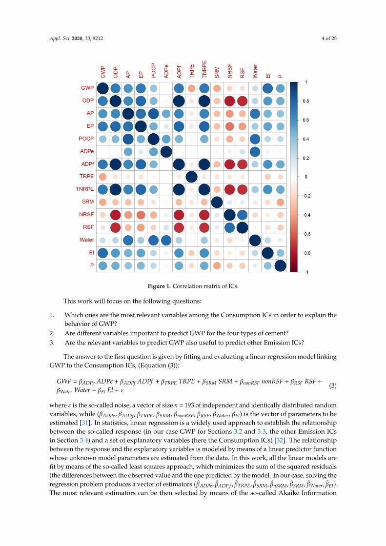
A preliminary analysis on the correlation matrix, performed to study relations between variables,is given in Figure 1. Positive and negative correlations are displayed in blue and red color, respectively,while the intensity of the color of each circle and its size is proportional to the absolute value ofthe corresponding correlation coefficient. Figure 1 shows that ODP, ADPf and TNRPE are pairwiseperfectly correlated, that is, the corresponding correlation coefficient is equal to 1. This implies thatthese variables match deterministically, up to a multiplicative factor. For this reason, ODP and TNRPEare discarded in the further analysis. The remaining ICs have been used as independent variables andsplit into two groups, “Emissions” and “Consumption” (Table 2).

Table 2. Classes of ICs.

Emission Consumption

GWP, AP, EP, POCP, P ADPe, ADPf, TRPE, SRM, nonRSF, RSF, Water, El

Appl. Sci. 2020, 10, 8212 4 of 25

Appl. Sci. 2020, 10, x; doi: FOR PEER REVIEW 4 of 25

Figure 1. Correlation matrix of ICs.

Table 2. Classes of ICs.

Emission Consumption GWP, AP, EP, POCP, P ADPe, ADPf, TRPE, SRM, nonRSF, RSF, Water, El

This work will focus on the following questions:

1. Which ones are the most relevant variables among the Consumption ICs in order to explain the behavior of GWP?

2. Are different variables important to predict GWP for the four types of cement? 3. Are the relevant variables to predict GWP also useful to predict other Emission ICs?

The answer to the first question is given by fitting and evaluating a linear regression model linking GWP to the Consumption ICs, (Equation (3)):

GWP = βADPe ADPe + βADPf ADPf + βTRPE TRPE + βSRM SRM + βnonRSF nonRSF + βRSF RSF +

βWater Water + βEl El + ε

(3)

where ε is the so-called noise, a vector of size n = 193 of independent and identically distributed random variables, while (βADPe, βADPf, βTRPE, βSRM, βnonRSF, βRSF, βWater, βEl) is the vector of parameters to be estimated [31]. In statistics, linear regression is a widely used approach to establish the relationship between the so-called response (in our case GWP for Sections 3.2 and 3.3, the other Emission ICs in Section 3.4) and a set of explanatory variables (here the Consumption ICs) [32]. The relationship between the response and the explanatory variables is modeled by means of a linear predictor function whose unknown model parameters are estimated from the data. In this work, all the linear models are fit by means of the so-called least squares approach, which minimizes the sum of the squared residuals (the differences between the observed value and the one predicted by the model.

Figure 1. Correlation matrix of ICs.

This work will focus on the following questions:

1. Which ones are the most relevant variables among the Consumption ICs in order to explain thebehavior of GWP?

2. Are different variables important to predict GWP for the four types of cement?3. Are the relevant variables to predict GWP also useful to predict other Emission ICs?

The answer to the first question is given by fitting and evaluating a linear regression model linkingGWP to the Consumption ICs, (Equation (3)):

GWP = βADPe ADPe + βADPf ADPf + βTRPE TRPE + βSRM SRM + βnonRSF nonRSF + βRSF RSF +

βWater Water + βEl El + ε(3)

where ε is the so-called noise, a vector of size n = 193 of independent and identically distributed randomvariables, while (βADPe, βADPf, βTRPE, βSRM, βnonRSF, βRSF, βWater, βEl) is the vector of parameters to beestimated [31]. In statistics, linear regression is a widely used approach to establish the relationshipbetween the so-called response (in our case GWP for Sections 3.2 and 3.3, the other Emission ICsin Section 3.4) and a set of explanatory variables (here the Consumption ICs) [32]. The relationshipbetween the response and the explanatory variables is modeled by means of a linear predictor functionwhose unknown model parameters are estimated from the data. In this work, all the linear models arefit by means of the so-called least squares approach, which minimizes the sum of the squared residuals(the differences between the observed value and the one predicted by the model. In our case, solving theregression problem produces a vector of estimators (βADPe, βADP f , βTRPE, βSRM, βnSRM, βSRM, βWater, βEl).The most relevant estimators can be then selected by means of the so-called Akaike Information

Appl. Sci. 2020, 10, 8212 5 of 25

Criterion (AIC) [32]. This procedure results in a model where only statistically significant variablesin terms of the highest variances are selected, while the others are iteratively discarded. A modelvalidation is then performed by means of a 10-fold cross validation procedure [31] to assess andcompare the accuracy of the two models. Cross validation evaluates the accuracy of a predictivemodel, estimating its ability to predict new data. In the k-fold cross validation, the original datasetis randomly partitioned into k subsamples of equal size. Then, one subsample (the validation data)is used to test the model obtained by using the remaining k-1 subsamples (the so-called trainingdata). This procedure is then repeated k times and averaged, so that all the observations are usedfor both validation and testing. The measure of the accuracy of each method is provided by the rootmean square error, the risk function which measures the square root of the average squared differencebetween observations and the estimated values [31].

As far as the second question is concerned, it is now investigated if different types of cementinfluence GWP in different ways and, consequently, if the statistical model’s accuracy can be improvedby fitting a separate regression model for each class. These regression models can be expressed asEquation (4):

GWP = βADPe;i ADPei + βADPf;i ADPfi + βTRPE;i TRPEi + βSRM;i SRMi + βnonRSF;i nonRSFi + βRSF;i

RSFi + βWater;i Wateri + βEl;i Eli + εi(4)

where i = I, II, III, IV and solving the regression model produces estimates for the set of parameters(βADPe;i, βADP f ;i, βTRPE;i, βSRM;i, βnonRSF;i, βWater;i, βEl;i), i = I, . . . , IV. It is also relevant to check if sometypes of cement behave differently in terms of the regression models and relevant variables. Again,10-fold cross validation procedures [31] are used to compare the results and to verify how accurateeach predictive model is.

Regarding the third question, a multiple linear regression using the full set of Consumption ICsis performed and used to evaluate two alternative models. The first alternative model uses as inputvariables only the ones selected for GWP. The other alternative model develops different variables foreach Emission IC, by means of the AIC criterion. If sufficiently accurate, the first model would allowthe producer to focus on the same subset of variables to control jointly all the emissions. If it is not thecase, the second model establishes which Consumption ICs are relevant to predict other emissions thanGWP. Also in this case, a 10-fold cross validation procedure has been applied to compare the accuracyof the models. The statistical analysis has been performed within the R Cran environment [33] and thesupport of additional packages [34,35].

3. Results

In this section, details concerning the performed data analysis are presented and discussed toanswer the questions introduced in Section 2. In particular, Section 3.1 includes some preliminaryexploratory analysis. Section 3.2 concentrates on Question 1, by studying and comparing two models topredict GWP, the first model obtained by fitting a linear regression, and the second model by selectingthe most relevant variables by means of the AIC criterion. Section 3.3 is concerned with Question 2.For each type of cement, a linear regression is fit and then the most important Consumption ICs areselected by the AIC criterion. Analogies and differences shown by the models here developed and theones in Section 3.1 are then investigated. Section 3.4 is focused on the other Emission ICs and, then,on Question 3. For each type of Cement and for each Emission, three different models are studied andthen compared. The first model is a linear regression which uses all the available Consumption ICsto predict each emission. The second model is a linear regression where only the relevant variablesto GWP established in Section 3.2 are used. The third model selects the relevant variables for eachEmission by the AIC criterion. The three models are then examined and compared to establish whetherthe same Consumption ICs can be used to predict accurately all the Emissions or not.

Appl. Sci. 2020, 10, 8212 6 of 25

3.1. Exploratory Analysis

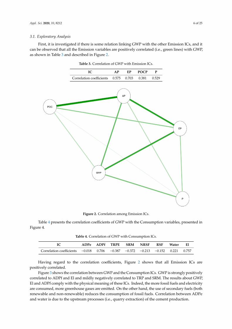
First, it is investigated if there is some relation linking GWP with the other Emission ICs, and itcan be observed that all the Emission variables are positively correlated (i.e., green lines) with GWP,as shown in Table 3 and described in Figure 2.

Table 3. Correlation of GWP with Emission ICs.

IC AP EP POCP P

Correlation coefficients 0.575 0.703 0.381 0.529

Appl. Sci. 2020, 10, x; doi: FOR PEER REVIEW 6 of 25

3.1. Exploratory Analysis

First, it is investigated if there is some relation linking GWP with the other Emission ICs, and it can be observed that all the Emission variables are positively correlated (i.e., green lines) with GWP, as shown in Table 3 and described in Figure 2.

Table 3. Correlation of GWP with Emission ICs.

IC AP EP POCP P Correlation coefficients 0.575 0.703 0.381 0.529

Table 4 presents the correlation coefficients of GWP with the Consumption variables, presented in Figure 4.

Table 4. Correlation of GWP with Consumption ICs.

IC ADPe ADPf TRPE SRM NRSF RSF Water El Correlation coefficients −0.018 0.706 −0.387 −0.372 −0.213 −0.152 0.221 0.757

Having regard to the correlation coefficients, Figure 2 shows that all Emission ICs are positively correlated.

Figure 2. Correlation among Emission ICs.

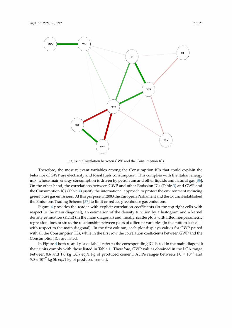
Figure 3 shows the correlation between GWP and the Consumption ICs. GWP is strongly positively correlated to ADPf and El and mildly negatively correlated to TRP and SRM. The results about GWP, El and ADPf comply with the physical meaning of these ICs. Indeed, the more fossil fuels and electricity are consumed, more greenhouse gases are emitted. On the other hand, the use of secondary fuels (both renewable and non-renewable) reduces the consumption of fossil fuels. Correlation between ADPe and water is due to the upstream processes (i.e., quarry extraction) of the cement production.

Figure 2. Correlation among Emission ICs.

Table 4 presents the correlation coefficients of GWP with the Consumption variables, presented inFigure 4.

Table 4. Correlation of GWP with Consumption ICs.

IC ADPe ADPf TRPE SRM NRSF RSF Water El

Correlation coefficients −0.018 0.706 −0.387 −0.372 −0.213 −0.152 0.221 0.757

Having regard to the correlation coefficients, Figure 2 shows that all Emission ICs arepositively correlated.

Figure 3 shows the correlation between GWP and the Consumption ICs. GWP is strongly positivelycorrelated to ADPf and El and mildly negatively correlated to TRP and SRM. The results about GWP,El and ADPf comply with the physical meaning of these ICs. Indeed, the more fossil fuels and electricityare consumed, more greenhouse gases are emitted. On the other hand, the use of secondary fuels (bothrenewable and non-renewable) reduces the consumption of fossil fuels. Correlation between ADPeand water is due to the upstream processes (i.e., quarry extraction) of the cement production.

Appl. Sci. 2020, 10, 8212 7 of 25Appl. Sci. 2020, 10, x; doi: FOR PEER REVIEW 7 of 25

Figure 3. Correlation between GWP and the Consumption ICs.

Therefore, the most relevant variables among the Consumption ICs that could explain the behavior of GWP are electricity and fossil fuels consumption. This complies with the Italian energy mix, whose main energy consumption is driven by petroleum and other liquids and natural gas [36]. On the other hand, the correlations between GWP and other Emission ICs (Table 3) and GWP and the Consumption ICs (Table 4) justify the international approach to protect the environment reducing greenhouse gas emissions. At this purpose, in 2003 the European Parliament and the Council established the Emissions Trading Scheme [37] to limit or reduce greenhouse gas emissions.

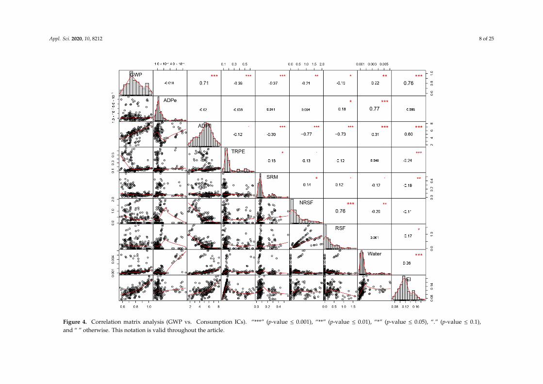
Figure 4 provides the reader with explicit correlation coefficients (in the top-right cells with respect to the main diagonal), an estimation of the density function by a histogram and a kernel density estimation (KDE) (in the main diagonal) and, finally, scatterplots with fitted nonparametric regression lines to stress the relationship between pairs of different variables (in the bottom-left cells with respect to the main diagonal). In the first column, each plot displays values for GWP paired with all the Consumption ICs, while in the first row the correlation coefficients between GWP and the Consumption ICs are listed.

In Figure 4 both x- and y- axis labels refer to the corresponding iCs listed in the main diagonal; their units comply with those listed in Table 1. Therefore, GWP values obtained in the LCA range between 0.6 and 1.0 kg CO2 eq./1 kg of produced cement; ADPe ranges between 1.0 × 10−7 and 5.0 × 10−7 kg Sb eq./1 kg of produced cement.

Figure 3. Correlation between GWP and the Consumption ICs.

Therefore, the most relevant variables among the Consumption ICs that could explain thebehavior of GWP are electricity and fossil fuels consumption. This complies with the Italian energymix, whose main energy consumption is driven by petroleum and other liquids and natural gas [36].On the other hand, the correlations between GWP and other Emission ICs (Table 3) and GWP andthe Consumption ICs (Table 4) justify the international approach to protect the environment reducinggreenhouse gas emissions. At this purpose, in 2003 the European Parliament and the Council establishedthe Emissions Trading Scheme [37] to limit or reduce greenhouse gas emissions.

Figure 4 provides the reader with explicit correlation coefficients (in the top-right cells withrespect to the main diagonal), an estimation of the density function by a histogram and a kerneldensity estimation (KDE) (in the main diagonal) and, finally, scatterplots with fitted nonparametricregression lines to stress the relationship between pairs of different variables (in the bottom-left cellswith respect to the main diagonal). In the first column, each plot displays values for GWP pairedwith all the Consumption ICs, while in the first row the correlation coefficients between GWP and theConsumption ICs are listed.

In Figure 4 both x- and y- axis labels refer to the corresponding iCs listed in the main diagonal;their units comply with those listed in Table 1. Therefore, GWP values obtained in the LCA rangebetween 0.6 and 1.0 kg CO2 eq./1 kg of produced cement; ADPe ranges between 1.0 × 10−7 and5.0 × 10−7 kg Sb eq./1 kg of produced cement.

Appl. Sci. 2020, 10, 8212 8 of 25Appl. Sci. 2020, 10, x; doi: FOR PEER REVIEW 8 of 25

Figure 4. Correlation matrix analysis (GWP vs. Consumption ICs). “***” (p-value ≤ 0.001), “**” (p-value ≤ 0.01), “*” (p-value ≤ 0.05), “.” (p-value ≤ 0.1), and “ “ otherwise. This notation is valid throughout the article.

Figure 4. Correlation matrix analysis (GWP vs. Consumption ICs). “***” (p-value ≤ 0.001), “**” (p-value ≤ 0.01), “*” (p-value ≤ 0.05), “.” (p-value ≤ 0.1),and “ ” otherwise. This notation is valid throughout the article.

Appl. Sci. 2020, 10, 8212 9 of 25

3.2. Linear Regression and Variable Selection for GWP

In this Section two predictive models for GWP are fit. The first model is a linear regression whereGWP is the scalar response and the Consumption ICs are the input variables. All variables have beenpreliminarily normalized to simplify the interpretation. The estimated coefficients are listed in Table 5,together with the related standard deviations (St. dev.) and the corresponding significance for thep-values associated to the significance test of the model.

Table 5. Linear regression summary (GWP vs. Consumption ICs).

ICsLinear Regression (GWP vs. Consumption ICs)

Coefficients St. Dev. p-Value

ADPe −0.127 0.038 **ADPf 1.503 0.077 ***TRPE −0.082 0.026 **SRM 0.532 0.025 **NRSF 0.531 0.052 ***RSF 0.563 0.039 ***

Water −0.017 0.041El −0.006 0.043

“***” (p-value ≤ 0.001), “**” (p-value ≤ 0.01) and “ ” otherwise.

To develop the second model, an AIC backward selection procedure is then performed on thelinear regression, to find the best subset of Consumption ICs to accurately predict GWP, leading to themodel described in Table 6.

Table 6. Linear regression model summary (after variable selection).

ICsLinear Regression (GWP vs. Selected Consumption ICs)

Coefficients St. Dev. p-Value

ADPe −0.140 0.022 ***ADPf 1.486 0.044 ***TRPE −0.085 0.025 ***SRM 0.527 0.024 **NRSF 0.527 0.040 ***RSF 0.558 0.037 ***

“***” (p-value ≤ 0.001), “**” (p-value ≤ 0.01).

Then, a 10-fold cross-validation procedure is performed to compare the two models. The rootmean square errors (RMSE) are computed by Equations (5) and (6):

RMSElin = ( 1n

n∑i=1

(GWPi − βlinADPeADPei − β

linADP f ADP fi − βlin

TRPETRPEi − βlinSRMSRMi

−βlinNRSFNRSFi − β

linRSFRSFi − β

linWaterWateri − β

linELELi)

2)

1/2(5)

RMSEAIC = ( 1n

n∑i=1

(GWPi − βAICADPeADPei − β

AICADP f ADP fi − βAIC

TRPETRPEi − βAICSRMSRMi

−βAICNRSFNRSFi − β

AICRSFRSFi − β

AICWaterWateri − β

AICEL ELi)

2)

1/2(6)

for the linear and AIC model, respectively. The sample size n = 193 is the number of observations,

while(βlin

ADPe, βlinADP f , βlin

TRPE, βlinSRM, βlin

NRSF, βlinRSF, βlin

Water, βlinE

), and

(βAIC

ADPe, βAICADP f , βAIC

TRPE, βAICSRM, βAIC

NRSF, βAICRSF

)are the estimated parameters with the linear model and then selected by the AIC criterion, respectively.Recall that the RMSE is a risk function aimed to measure the discrepancy between the observations

Appl. Sci. 2020, 10, 8212 10 of 25

and the corresponding estimated values. In Table 7 RMSElin is higher than RMSEAIC, thus the variablereduction produces a more accurate model.

Table 7. Comparison of RMSE between the two models.

Model RMSE

Linear 0.313AIC 0.305

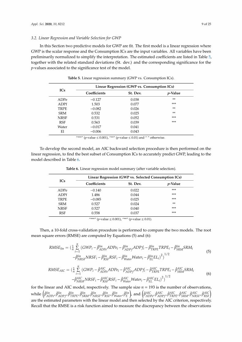
Finally, Figure 5 describes the size of each regression slope coefficient, after the variable selection.The highest contribution to GWP is given by ADPf. This result complies with the release of carbondioxide into the atmosphere by burning of fossil fuels [38–40].

Appl. Sci. 2020, 10, x; doi: FOR PEER REVIEW 10 of 25

Table 7. Comparison of RMSE between the two models.

Model RMSE Linear 0.313

AIC 0.305

Finally, Figure 5 describes the size of each regression slope coefficient, after the variable selection. The highest contribution to GWP is given by ADPf. This result complies with the release of carbon dioxide into the atmosphere by burning of fossil fuels [38–40].

Figure 5. Size of the coefficients (AIC selected components—absolute values).

In answer to Question 1, the most relevant variables among the Consumption ICs to predict GWP are ADPf, NRSF and RSF. The energy-intensive industry of cement manufacturing can motivate this variable selection: all these ICs quantify the energy, mainly fossil but also alternative, spent in the process. This result complies with the efforts to implement in the cement sector different management systems, process-integrated techniques and end-of-pipe measures identified as Best Available Techniques (BAT) to have environmental benefits (e.g., thermal energy optimization techniques in the kiln system; reduction of electrical energy use; recovery of excess heat from the process and cogeneration of steam and electrical power) [41].

3.3. Linear Regression and Variable Selection for Each Type of Cement

The different types of cement are now studied separately to evaluate their impact on GWP. Figure 6, which contains the scatterplots related to GWP and the Consumption ICs, shows that the points associated to the class CEM I (in blue) are isolated in the GWP scatterplots with respect to the data belonging to the other types. Moreover, the environmental impacts of CEM I are higher than other investigated cement types: both the qualitative and the quantitative observed trends suggest investigating whether predictive models built separately for each class (type of cement) could achieve more accurate predictions for GWP. Furthermore, it is of extreme interest to check if different variables result to be important for each separate class with respect to the ones selected for the whole dataset. Figure 6 contains a matrix of scatterplots used to visualize the relationship between pairs of variables, all listed in the main diagonal. For each scatterplot, the variables in the x-axis (y-axis, respectively) can be found in the entry belonging to the main diagonal in the same column (row, respectively). The units of each axis label are listed in Table 1.

Figure 5. Size of the coefficients (AIC selected components—absolute values).

In answer to Question 1, the most relevant variables among the Consumption ICs to predict GWPare ADPf, NRSF and RSF. The energy-intensive industry of cement manufacturing can motivate thisvariable selection: all these ICs quantify the energy, mainly fossil but also alternative, spent in the process.This result complies with the efforts to implement in the cement sector different management systems,process-integrated techniques and end-of-pipe measures identified as Best Available Techniques (BAT)to have environmental benefits (e.g., thermal energy optimization techniques in the kiln system;reduction of electrical energy use; recovery of excess heat from the process and cogeneration of steamand electrical power) [41].

3.3. Linear Regression and Variable Selection for Each Type of Cement

The different types of cement are now studied separately to evaluate their impact on GWP.Figure 6, which contains the scatterplots related to GWP and the Consumption ICs, shows that thepoints associated to the class CEM I (in blue) are isolated in the GWP scatterplots with respect to thedata belonging to the other types. Moreover, the environmental impacts of CEM I are higher thanother investigated cement types: both the qualitative and the quantitative observed trends suggestinvestigating whether predictive models built separately for each class (type of cement) could achievemore accurate predictions for GWP. Furthermore, it is of extreme interest to check if different variablesresult to be important for each separate class with respect to the ones selected for the whole dataset.Figure 6 contains a matrix of scatterplots used to visualize the relationship between pairs of variables,all listed in the main diagonal. For each scatterplot, the variables in the x-axis (y-axis, respectively) canbe found in the entry belonging to the main diagonal in the same column (row, respectively). The unitsof each axis label are listed in Table 1.

Appl. Sci. 2020, 10, 8212 11 of 25Appl. Sci. 2020, 10, x; doi: FOR PEER REVIEW 11 of 25

Figure 6. Data and types of cement. (CEM I = blue, CEM II = red, CEM III = green, CEM IV = yellow).

Figure 6. Data and types of cement. (CEM I = blue, CEM II = red, CEM III = green, CEM IV = yellow).

Appl. Sci. 2020, 10, 8212 12 of 25

The dimensions of each class are given in Table 8.

Table 8. Dimensions of datasets related to each type of cement.

Cement Type Dimension of Classes

CEM I 44CEM II 84CEM III 4CEM IV 61

Due to the small number of observations, CEM III is filtered out.For each class, a linear regression is fit, where GWP corresponds to the scalar response and the

ICs to the explanatory variables. The estimated regression coefficients for CEM I, II, and IV are listedin Tables 9–11, respectively.

Table 9. Linear regression summary (GWP vs. Consumption ICs)—CEM I.

ICsLinear Regression (GWP vs. Consumption ICs) CEM I

Coefficients St. Dev. p-Value

ADPe 0.217 0.115ADPf 0.701 0.128 ***TRPE 0.105 0.115SRM 0.046 0.111NRSF 0.090 0.079RSF 0.181 0.061 **

Water −0.165 0.092 .El 0.052 0.050

“***” (p-value ≤ 0.001), “**” (p-value ≤ 0.01), “.” (p-value ≤ 0.1), and “ ” otherwise.

Table 10. Linear regression summary (GWP vs. Consumption ICs)—CEM II.

ICsLinear Regression (GWP vs. Consumption ICs) CEM II

Coefficients St. Dev. p-Value

ADPe −0.052 0.099ADPf 1.237 0.156 ***TRPE −0.132 0.044 **SRM 0.052 0.148NRSF 0.389 0.104 ***RSF 0.414 0.077 ***

Water −0.029 0.089El −0.052 0.081

“***” (p-value ≤ 0.001), “**” (p-value ≤ 0.01) and “ ” otherwise.

Table 11. Linear regression summary (GWP vs. Consumption ICs)—CEM IV.

ICsLinear Regression (GWP vs. Consumption ICs) CEM IV

Coefficients St. Dev. p-Value

ADPe −0.049 0.045ADPf 1.234 0.157 ***TRPE −0.095 0.037 *SRM −0.007 0.032NRSF 0.420 0.091 ***RSF 0.412 0.082 ***

Water −0.016 0.062El −0.038 0.064

“***” (p-value ≤ 0.001), “*” (p-value ≤ 0.05), and “ ” otherwise.

Appl. Sci. 2020, 10, 8212 13 of 25

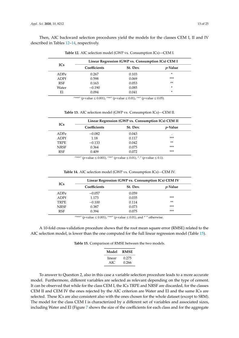
Then, AIC backward selection procedures yield the models for the classes CEM I, II and IVdescribed in Tables 12–14, respectively.

Table 12. AIC selection model (GWP vs. Consumption ICs)—CEM I.

ICsLinear Regression (GWP vs. Consumption ICs) CEM I

Coefficients St. Dev. p-Value

ADPe 0.267 0.103 *ADPf 0.598 0.069 ***RSF 0.163 0.053 **

Water −0.190 0.085 *El 0.094 0.041 *

“***” (p-value ≤ 0.001), “**” (p-value ≤ 0.01), “*” (p-value ≤ 0.05).

Table 13. AIC selection model (GWP vs. Consumption ICs)—CEM II.

ICsLinear Regression (GWP vs. Consumption ICs) CEM II

Coefficients St. Dev. p-Value

ADPe −0.082 0.043 .ADPf 1.18 0.117 ***TRPE −0.133 0.042 **NRSF 0.364 0.075 ***RSF 0.409 0.072 ***

“***” (p-value ≤ 0.001), “**” (p-value ≤ 0.01), “.” (p-value ≤ 0.1).

Table 14. AIC selection model (GWP vs. Consumption ICs)—CEM IV.

ICsLinear Regression (GWP vs. Consumption ICs) CEM IV

Coefficients St. Dev. p-Value

ADPe −0.057 0.059ADPf 1.173 0.035 ***TRPE −0.100 0.114 **NRSF 0.387 0.073 ***RSF 0.394 0.075 ***

“***” (p-value ≤ 0.001), “**” (p-value ≤ 0.01), and “ ” otherwise.

A 10-fold cross-validation procedure shows that the root mean square error (RMSE) related to theAIC selection model, is lower than the one computed for the full linear regression model (Table 15).

Table 15. Comparison of RMSE between the two models.

Model RMSE

linear 0.275AIC 0.266

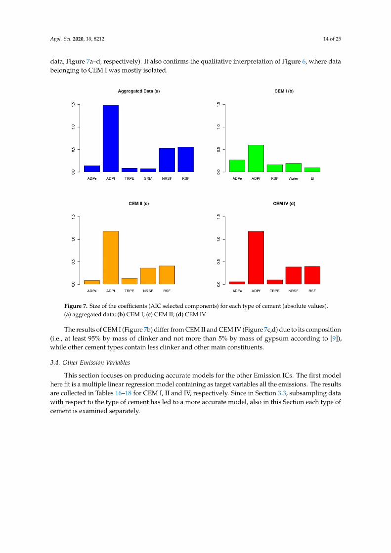
To answer to Question 2, also in this case a variable selection procedure leads to a more accuratemodel. Furthermore, different variables are selected as relevant depending on the type of cement.It can be observed that while for the class CEM I, the ICs TRPE and NRSF are discarded, for the classesCEM II and CEM IV the ones rejected by the AIC criterion are Water and El and the same ICs areselected. These ICs are also consistent also with the ones chosen for the whole dataset (except to SRM).The model for the class CEM I is characterized by a different set of variables and associated sizes,including Water and El (Figure 7 shows the size of the coefficients for each class and for the aggregate

Appl. Sci. 2020, 10, 8212 14 of 25

data, Figure 7a–d, respectively). It also confirms the qualitative interpretation of Figure 6, where databelonging to CEM I was mostly isolated.

Appl. Sci. 2020, 10, x FOR PEER REVIEW 14 of 25

data, Figure 7a,b–d, respectively). It also confirms the qualitative interpretation of Figure 6, where data belonging to CEM I was mostly isolated.

Figure 7. Size of the coefficients (AIC selected components) for each type of cement (absolute values). (a) aggregated data; (b) CEM I; (c) CEM II; (d) CEM IV.

The results of CEM I (Figure 7b) differ from CEM II and CEM IV (Figure 7c,d) due to its composition (i.e., at least 95% by mass of clinker and not more than 5% by mass of gypsum according to [9]), while other cement types contain less clinker and other main constituents.

3.4. Other Emission Variables

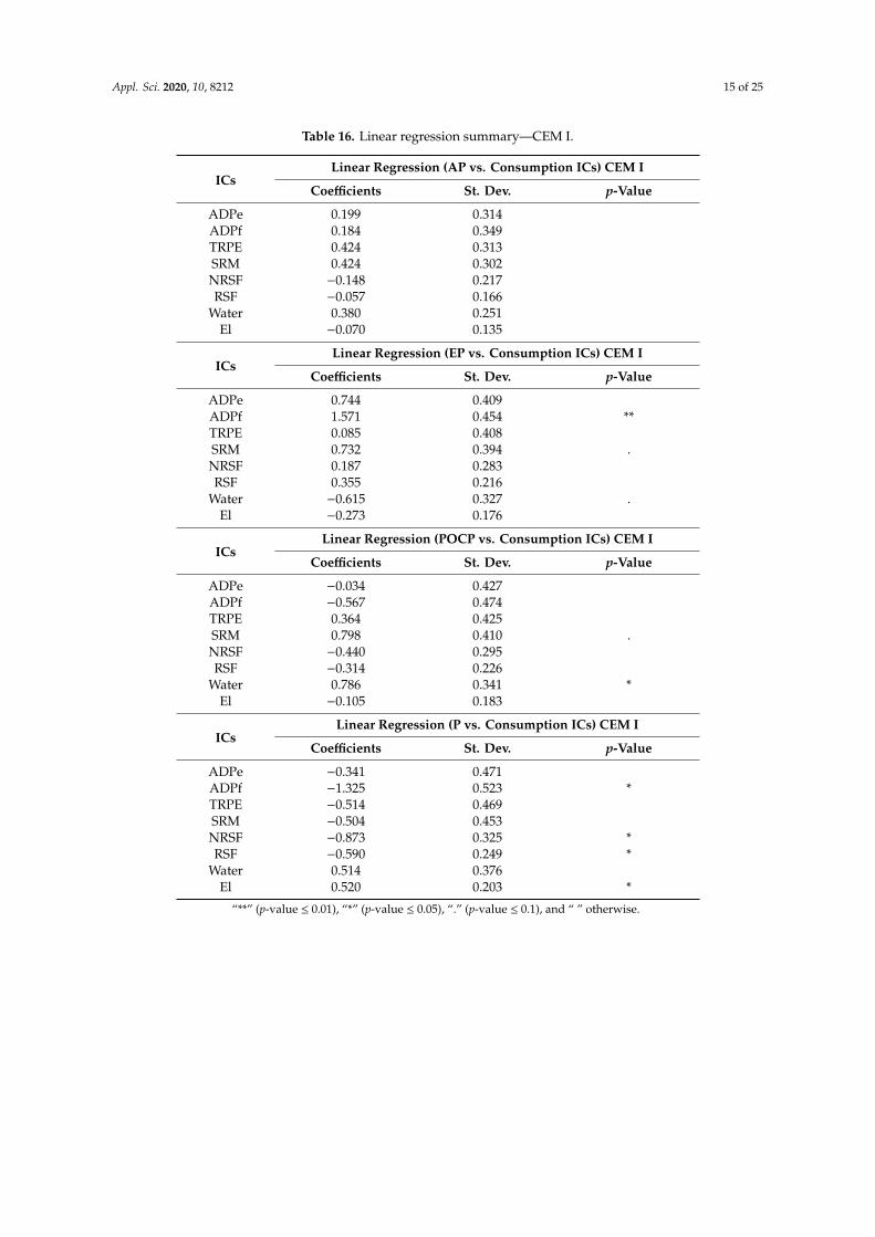
This section focuses on producing accurate models for the other Emission ICs. The first model here fit is a multiple linear regression model containing as target variables all the emissions. The results are collected in Tables 16–18 for CEM I, II and IV, respectively. Since in Section 3.3, subsampling data with respect to the type of cement has led to a more accurate model, also in this Section each type of cement is examined separately.

Figure 7. Size of the coefficients (AIC selected components) for each type of cement (absolute values).(a) aggregated data; (b) CEM I; (c) CEM II; (d) CEM IV.

The results of CEM I (Figure 7b) differ from CEM II and CEM IV (Figure 7c,d) due to its composition(i.e., at least 95% by mass of clinker and not more than 5% by mass of gypsum according to [9]),while other cement types contain less clinker and other main constituents.

3.4. Other Emission Variables

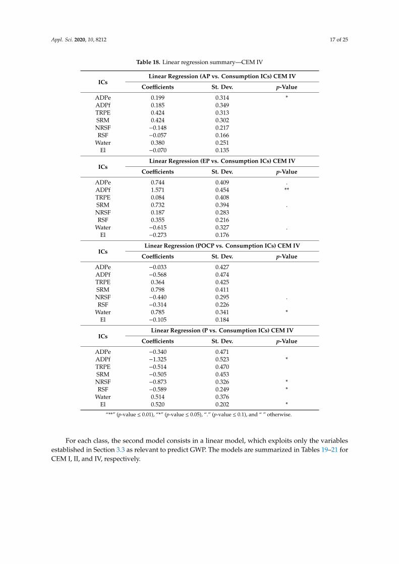
This section focuses on producing accurate models for the other Emission ICs. The first modelhere fit is a multiple linear regression model containing as target variables all the emissions. The resultsare collected in Tables 16–18 for CEM I, II and IV, respectively. Since in Section 3.3, subsampling datawith respect to the type of cement has led to a more accurate model, also in this Section each type ofcement is examined separately.

Appl. Sci. 2020, 10, 8212 15 of 25

Table 16. Linear regression summary—CEM I.

ICsLinear Regression (AP vs. Consumption ICs) CEM I

Coefficients St. Dev. p-Value

ADPe 0.199 0.314ADPf 0.184 0.349TRPE 0.424 0.313SRM 0.424 0.302NRSF −0.148 0.217RSF −0.057 0.166

Water 0.380 0.251El −0.070 0.135

ICsLinear Regression (EP vs. Consumption ICs) CEM I

Coefficients St. Dev. p-Value

ADPe 0.744 0.409ADPf 1.571 0.454 **TRPE 0.085 0.408SRM 0.732 0.394 .NRSF 0.187 0.283RSF 0.355 0.216

Water −0.615 0.327 .El −0.273 0.176

ICsLinear Regression (POCP vs. Consumption ICs) CEM I

Coefficients St. Dev. p-Value

ADPe −0.034 0.427ADPf −0.567 0.474TRPE 0.364 0.425SRM 0.798 0.410 .NRSF −0.440 0.295RSF −0.314 0.226

Water 0.786 0.341 *El −0.105 0.183

ICsLinear Regression (P vs. Consumption ICs) CEM I

Coefficients St. Dev. p-Value

ADPe −0.341 0.471ADPf −1.325 0.523 *TRPE −0.514 0.469SRM −0.504 0.453NRSF −0.873 0.325 *RSF −0.590 0.249 *

Water 0.514 0.376El 0.520 0.203 *

“**” (p-value ≤ 0.01), “*” (p-value ≤ 0.05), “.” (p-value ≤ 0.1), and “ ” otherwise.

Appl. Sci. 2020, 10, 8212 16 of 25

Table 17. Linear regression summary—CEM II.

ICsLinear Regression (AP vs. Consumption ICs) CEM II

Coefficients St. Dev. p-Value

ADPe 0.067 0.180ADPf 0.638 0.284 *TRPE −0.003 0.079SRM 0.175 0.269NRSF 0.116 0.189RSF 0.017 0.140

Water 0.605 0.160 ***El −0.160 0.147

ICsLinear Regression (EP vs. Consumption ICs) CEM II

Coefficients St. Dev. p-Value

ADPe 0.084 0.187ADPf 1.709 0.296 ***TRPE 0.145 0.083 .SRM 0.627 0.281 *NRSF 0.411 0.197 *RSF 0.427 0.146 **

Water −0.025 0.168El −0.394 0.153 *

ICsLinear Regression (POCP vs. Consumption ICs) CEM II

Coefficients St. Dev. p-Value

ADPe −0.178 0.199ADPf −0.289 0.314TRPE −0.033 0.088SRM 0.495 0.298 .NRSF 0.094 0.209RSF −0.065 0.155

Water 0.950 0.178 ***El −0.296 0.162 .

ICsLinear Regression (P vs. Consumption ICs) CEM II

Coefficients St. Dev. p-Value

ADPe −0.010 0.249ADPf −0.045 0.393TRPE −0.084 0.110SRM −0.022 0.372NRSF 0.022 0.261RSF −0.287 0.193

Water 0.141 0.222El −0.028 0.203

“***” (p-value ≤ 0.001), “**” (p-value ≤ 0.01), “*” (p-value ≤ 0.05), “.” (p-value ≤ 0.1), and “ ” otherwise.

Appl. Sci. 2020, 10, 8212 17 of 25

Table 18. Linear regression summary—CEM IV

ICsLinear Regression (AP vs. Consumption ICs) CEM IV

Coefficients St. Dev. p-Value

ADPe 0.199 0.314 *ADPf 0.185 0.349TRPE 0.424 0.313SRM 0.424 0.302NRSF −0.148 0.217RSF −0.057 0.166

Water 0.380 0.251El −0.070 0.135

ICsLinear Regression (EP vs. Consumption ICs) CEM IV

Coefficients St. Dev. p-Value

ADPe 0.744 0.409 .ADPf 1.571 0.454 **TRPE 0.084 0.408SRM 0.732 0.394 .NRSF 0.187 0.283RSF 0.355 0.216

Water −0.615 0.327 .El −0.273 0.176

ICsLinear Regression (POCP vs. Consumption ICs) CEM IV

Coefficients St. Dev. p-Value

ADPe −0.033 0.427ADPf −0.568 0.474TRPE 0.364 0.425SRM 0.798 0.411NRSF −0.440 0.295 .RSF −0.314 0.226

Water 0.785 0.341 *El −0.105 0.184

ICsLinear Regression (P vs. Consumption ICs) CEM IV

Coefficients St. Dev. p-Value

ADPe −0.340 0.471ADPf −1.325 0.523 *TRPE −0.514 0.470SRM −0.505 0.453NRSF −0.873 0.326 *RSF −0.589 0.249 *

Water 0.514 0.376El 0.520 0.202 *

“**” (p-value ≤ 0.01), “*” (p-value ≤ 0.05), “.” (p-value ≤ 0.1), and “ ” otherwise.

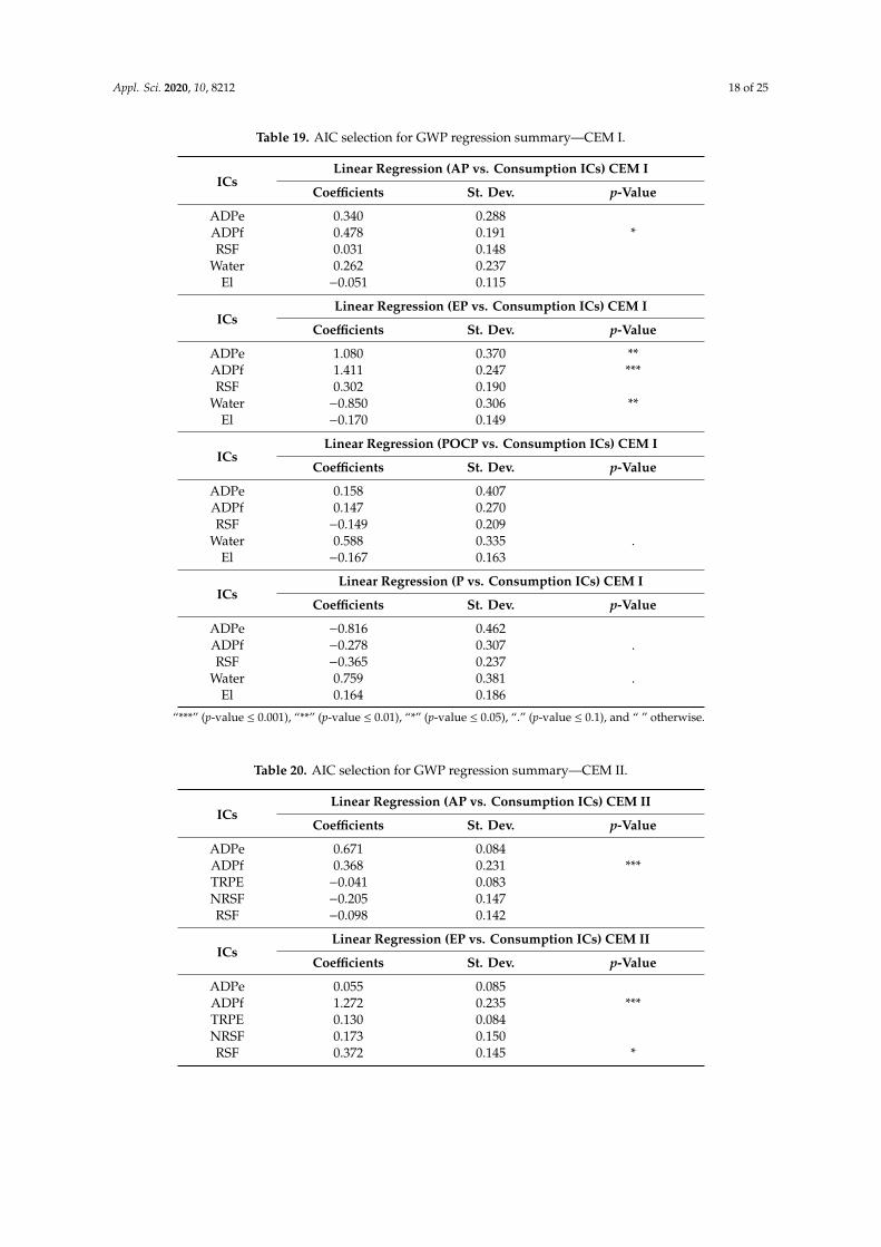
For each class, the second model consists in a linear model, which exploits only the variablesestablished in Section 3.3 as relevant to predict GWP. The models are summarized in Tables 19–21 forCEM I, II, and IV, respectively.

Appl. Sci. 2020, 10, 8212 18 of 25

Table 19. AIC selection for GWP regression summary—CEM I.

ICsLinear Regression (AP vs. Consumption ICs) CEM I

Coefficients St. Dev. p-Value

ADPe 0.340 0.288ADPf 0.478 0.191 *RSF 0.031 0.148

Water 0.262 0.237El −0.051 0.115

ICsLinear Regression (EP vs. Consumption ICs) CEM I

Coefficients St. Dev. p-Value

ADPe 1.080 0.370 **ADPf 1.411 0.247 ***RSF 0.302 0.190

Water −0.850 0.306 **El −0.170 0.149

ICsLinear Regression (POCP vs. Consumption ICs) CEM I

Coefficients St. Dev. p-Value

ADPe 0.158 0.407ADPf 0.147 0.270RSF −0.149 0.209

Water 0.588 0.335 .El −0.167 0.163

ICsLinear Regression (P vs. Consumption ICs) CEM I

Coefficients St. Dev. p-Value

ADPe −0.816 0.462ADPf −0.278 0.307 .RSF −0.365 0.237

Water 0.759 0.381 .El 0.164 0.186

“***” (p-value ≤ 0.001), “**” (p-value ≤ 0.01), “*” (p-value ≤ 0.05), “.” (p-value ≤ 0.1), and “ ” otherwise.

Table 20. AIC selection for GWP regression summary—CEM II.

ICsLinear Regression (AP vs. Consumption ICs) CEM II

Coefficients St. Dev. p-Value

ADPe 0.671 0.084ADPf 0.368 0.231 ***TRPE −0.041 0.083NRSF −0.205 0.147RSF −0.098 0.142

ICsLinear Regression (EP vs. Consumption ICs) CEM II

Coefficients St. Dev. p-Value

ADPe 0.055 0.085ADPf 1.272 0.235 ***TRPE 0.130 0.084NRSF 0.173 0.150RSF 0.372 0.145 *

Appl. Sci. 2020, 10, 8212 19 of 25

Table 20. Cont.

ICsLinear Regression (AP vs. Consumption ICs) CEM II

Coefficients St. Dev. p-Value

ADPe 0.766 0.101ADPf −0.176 0.278 ***TRPE −0.091 0.100NRSF −0.429 0.178 *RSF −0.246 0.171

ICsLinear Regression (P vs. Consumption ICs) CEM II

Coefficients St. Dev. p-Value

ADPe 0.132 0.107ADPf −0.103 0.293TRPE −0.094 0.105NRSF −0.049 0.187RSF −0.315 0.181 .

“***” (p-value ≤ 0.001), “*” (p-value ≤ 0.05), “.” (p-value ≤ 0.1), and “ ” otherwise.

Table 21. AIC selection for GWP regression summary—CEM IV.

ICsLinear Regression (AP vs. Consumption ICs) CEM IV

Coefficients St. Dev. p-Value

ADPe 0.379 0.071 ***ADPf 0.828 0.235 ***TRPE −0.015 0.063NRSF 0.094 0.150RSF 0.135 0.154

ICsLinear Regression (EP vs. Consumption ICs) CEM IV

Coefficients St. Dev. p-Value

ADPe 0.211 0.059 ***ADPf 0.858 0.195 ***TRPE −0.037 0.052NRSF −0.006 0.124RSF 0.178 0.129

ICsLinear Regression (POCP vs. Consumption ICs) CEM IV

Coefficients St. Dev. p-Value

ADPe 0.379 0.096ADPf 0.357 0.314 ***TRPE −0.028 0.084NRSF −0.115 0.200RSF 0.040 0.207

ICsLinear Regression (P vs. Consumption ICs) CEM IV

Coefficients St. Dev. p-Value

ADPe 0.071 0.095ADPf 1.021 0.314 **TRPE −0.172 0.084 *NRSF 0.292 0.200RSF 0.231 0.206

“***” (p-value ≤ 0.001), “**” (p-value ≤ 0.01), “*” (p-value ≤ 0.05), and “ ” otherwise.

Appl. Sci. 2020, 10, 8212 20 of 25

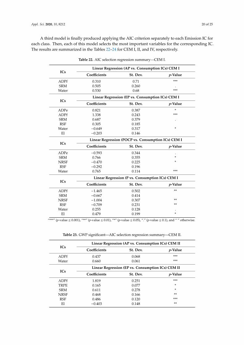
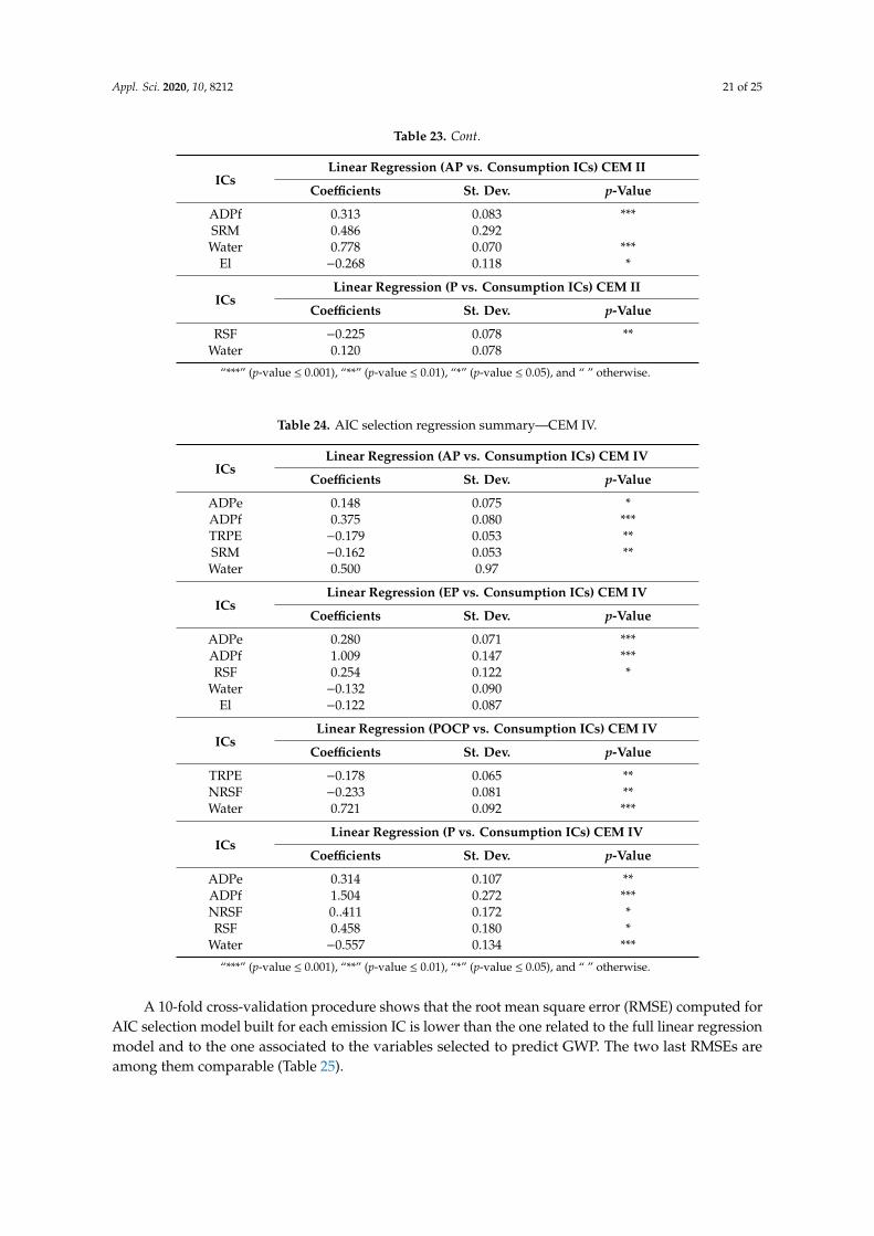
A third model is finally produced applying the AIC criterion separately to each Emission IC foreach class. Then, each of this model selects the most important variables for the corresponding IC.The results are summarized in the Tables 22–24 for CEM I, II, and IV, respectively.

Table 22. AIC selection regression summary—CEM I.

ICsLinear Regression (AP vs. Consumption ICs) CEM I

Coefficients St. Dev. p-Value

ADPf 0.310 0.71 ***SRM 0.505 0.260 .Water 0.530 0.68 ***

ICsLinear Regression (EP vs. Consumption ICs) CEM I

Coefficients St. Dev. p-Value

ADPe 0.821 0.387 *ADPf 1.338 0.243 ***SRM 0.687 0.379 .RSF 0.305 0.185

Water −0.649 0.317 *El −0.203 0.146

ICsLinear Regression (POCP vs. Consumption ICs) CEM I

Coefficients St. Dev. p-Value

ADPe −0.593 0.344 .SRM 0.766 0.355 *NRSF −0.470 0.225 *RSF −0.292 0.196

Water 0.765 0.114 ***

ICsLinear Regression (P vs. Consumption ICs) CEM I

Coefficients St. Dev. p-Value

ADPf −1.465 0.502 **SRM −0.667 0.414NRSF −1.004 0.307 **RSF −0.709 0.231 **

Water 0.255 0.128 .El 0.479 0.199 *

“***” (p-value ≤ 0.001), “**” (p-value ≤ 0.01), “*” (p-value ≤ 0.05), “.” (p-value ≤ 0.1), and “ ” otherwise.

Table 23. GWP significant—AIC selection regression summary—CEM II.

ICsLinear Regression (AP vs. Consumption ICs) CEM II

Coefficients St. Dev. p-Value

ADPf 0.437 0.068 ***Water 0.660 0.061 ***

ICsLinear Regression (EP vs. Consumption ICs) CEM II

Coefficients St. Dev. p-Value

ADPf 1.819 0.251 ***TRPE 0.165 0.077 *SRM 0.611 0.278 *NRSF 0.468 0.166 **RSF 0.486 0.120 ***El −0.403 0.148 **

Appl. Sci. 2020, 10, 8212 21 of 25

Table 23. Cont.

ICsLinear Regression (AP vs. Consumption ICs) CEM II

Coefficients St. Dev. p-Value

ADPf 0.313 0.083 ***SRM 0.486 0.292Water 0.778 0.070 ***

El −0.268 0.118 *

ICsLinear Regression (P vs. Consumption ICs) CEM II

Coefficients St. Dev. p-Value

RSF −0.225 0.078 **Water 0.120 0.078

“***” (p-value ≤ 0.001), “**” (p-value ≤ 0.01), “*” (p-value ≤ 0.05), and “ ” otherwise.

Table 24. AIC selection regression summary—CEM IV.

ICsLinear Regression (AP vs. Consumption ICs) CEM IV

Coefficients St. Dev. p-Value

ADPe 0.148 0.075 *ADPf 0.375 0.080 ***TRPE −0.179 0.053 **SRM −0.162 0.053 **Water 0.500 0.97

ICsLinear Regression (EP vs. Consumption ICs) CEM IV

Coefficients St. Dev. p-Value

ADPe 0.280 0.071 ***ADPf 1.009 0.147 ***RSF 0.254 0.122 *

Water −0.132 0.090El −0.122 0.087

ICsLinear Regression (POCP vs. Consumption ICs) CEM IV

Coefficients St. Dev. p-Value

TRPE −0.178 0.065 **NRSF −0.233 0.081 **Water 0.721 0.092 ***

ICsLinear Regression (P vs. Consumption ICs) CEM IV

Coefficients St. Dev. p-Value

ADPe 0.314 0.107 **ADPf 1.504 0.272 ***NRSF 0..411 0.172 *RSF 0.458 0.180 *

Water −0.557 0.134 ***

“***” (p-value ≤ 0.001), “**” (p-value ≤ 0.01), “*” (p-value ≤ 0.05), and “ ” otherwise.

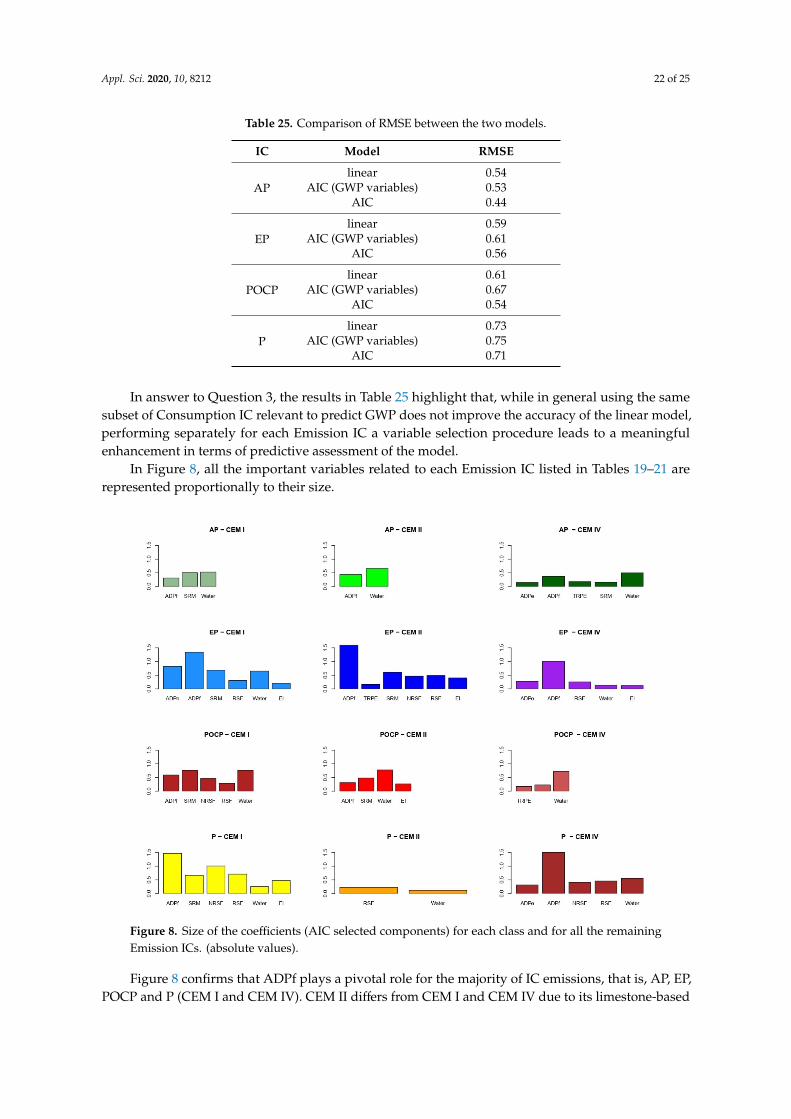
A 10-fold cross-validation procedure shows that the root mean square error (RMSE) computed forAIC selection model built for each emission IC is lower than the one related to the full linear regressionmodel and to the one associated to the variables selected to predict GWP. The two last RMSEs areamong them comparable (Table 25).

Appl. Sci. 2020, 10, 8212 22 of 25

Table 25. Comparison of RMSE between the two models.

IC Model RMSE

APlinear 0.54

AIC (GWP variables) 0.53AIC 0.44

EPlinear 0.59

AIC (GWP variables) 0.61AIC 0.56

POCPlinear 0.61

AIC (GWP variables) 0.67AIC 0.54

Plinear 0.73

AIC (GWP variables) 0.75AIC 0.71

In answer to Question 3, the results in Table 25 highlight that, while in general using the samesubset of Consumption IC relevant to predict GWP does not improve the accuracy of the linear model,performing separately for each Emission IC a variable selection procedure leads to a meaningfulenhancement in terms of predictive assessment of the model.

In Figure 8, all the important variables related to each Emission IC listed in Tables 19–21 arerepresented proportionally to their size.

Appl. Sci. 2020, 10, x FOR PEER REVIEW 22 of 25

Figure 8. Size of the coefficients (AIC selected components) for each class and for all the remaining Emission ICs. (absolute values).

Figure 8 confirms that ADPf plays a pivotal role for the majority of IC emissions, that is, AP, EP, POCP and P (CEM I and CEM IV). CEM II differs from CEM I and CEM IV due to its limestone-based composition; particularly, POCP CEM II has its highest correlation with the Water consumption IC. It is confirmed by the upstream processes necessary to quarry natural raw materials.

4. Discussion

Due to a dependence on fossil fuels and the calcination of raw materials, the cement industry generates about 5% of global greenhouse gas emissions. Within this framework, several efforts are on-going to protect the environment and increase energy efficiency using renewable resources or alternative fuels. In order to analyze comparable environmental performances, cement companies are conducting life cycle assessment of their “from cradle to gate” processes in order to identify the best strategies to meet the need for sustainable development.

In this study, having regard to the European approach compliant with the standard EN 15804, the environmental impacts of 193 different recipes of gray cement produced in Italy from 2014 to 2019 have been assessed. Fifteen different impact categories have been considered and split into two classes, “Emissions” and “Consumption”. One of the main results of this work concerns the identification of the significant Consumption ICs to predict the behavior of Emission ICs, In particular, the target of this paper consists in answering to the following questions:

1. Which ones are the most relevant variables among the Consumption ICs in order to explain the behavior of GWP?

2. Are different variables important to predict GWP for the four types of cement? 3. Are the relevant variables to predict GWP also useful to predict other Emission ICs?

Figure 8. Size of the coefficients (AIC selected components) for each class and for all the remainingEmission ICs. (absolute values).

Figure 8 confirms that ADPf plays a pivotal role for the majority of IC emissions, that is, AP, EP,POCP and P (CEM I and CEM IV). CEM II differs from CEM I and CEM IV due to its limestone-based

Appl. Sci. 2020, 10, 8212 23 of 25

composition; particularly, POCP CEM II has its highest correlation with the Water consumption IC.It is confirmed by the upstream processes necessary to quarry natural raw materials.

4. Discussion

Due to a dependence on fossil fuels and the calcination of raw materials, the cement industrygenerates about 5% of global greenhouse gas emissions. Within this framework, several efforts areon-going to protect the environment and increase energy efficiency using renewable resources oralternative fuels. In order to analyze comparable environmental performances, cement companies areconducting life cycle assessment of their “from cradle to gate” processes in order to identify the beststrategies to meet the need for sustainable development.

In this study, having regard to the European approach compliant with the standard EN 15804,the environmental impacts of 193 different recipes of gray cement produced in Italy from 2014 to 2019have been assessed. Fifteen different impact categories have been considered and split into two classes,“Emissions” and “Consumption”. One of the main results of this work concerns the identification ofthe significant Consumption ICs to predict the behavior of Emission ICs, In particular, the target of thispaper consists in answering to the following questions:

1. Which ones are the most relevant variables among the Consumption ICs in order to explain thebehavior of GWP?

2. Are different variables important to predict GWP for the four types of cement?3. Are the relevant variables to predict GWP also useful to predict other Emission ICs?

As far as Question 1 is concerned, it is shown that the most important variable to predict thebehavior of GWP is ADPf (Figure 8), while NRSF and RSF are the two other most relevant consumptionvariables. To answer Question 2, a more accurate model is produced by fitting a linear regressionand applying the AIC criterion for different types of cement (i.e., CEM I, CEM II, CEM IV) separately.Also in this case, ADPf is proved to be the most important Consumption IC. However, scatterplotsrelated to GWP and the Consumption ICs show that the environmental performances of CEM I differfrom those of the other types, and their values are higher. Predictive models built separately for eachtype of cement revealed more accurate predictions for GWP. Finally, concerning Question 3, the authorsinvestigated if the relevant variables to predict GWP could predict other Emission ICs. In this case,it is shown that fitting separately regression models and selecting the most important variables leadsto more accurate predictions for all the other Emissions ICs (Table 25) in comparison to the standardlinear model or the one which uses the same Consumption ICs for GWP. Also in this case, ADPf isconfirmed to be a strong predictor in the models related to the emission variables AP, EP, POCP (forCEM I and CEM II), and P (for CEM I and CEM IV). Therefore, the obtained results underline theneed for policies and strategies that could reduce consumption of energy, both fossil and secondaryfuels, and justify the European policies about Emission trading and Best Available Techniques to beimplemented in the cement industry.

Author Contributions: Conceptualization, C.D. and L.M.; methodology, C.D.; software, C.D. and L.M.; validation,L.M. and C.D.; formal analysis, C.D.; data curation, L.M.; writing—original draft preparation, C.D. and L.M.;review and editing, C.D. and L.M. All authors have read and agreed to the published version of the manuscript.

Funding: This research received no external funding.

Conflicts of Interest: The authors declare no conflict of interest.

References

1. Miccoli, S.; Finucci, F.; Murro, R. Assessing project quality: A multidimensional approach. Adv. Mater. Res.2014, 1030–1032, 2519–2522. [CrossRef]

2. Miccoli, S.; Finucci, F.; Murro, R. Criteria and procedures for regional environmental regeneration: A Europeanstrategic project. Appl. Mech. Mater. 2014, 675–677, 401–405. [CrossRef]

Appl. Sci. 2020, 10, 8212 24 of 25

3. Anderson, T.R.; Hawkins, E.; Jones, P.D. CO2, the greenhouse effect and global warming: From the pioneeringwork of Arrhenius and callendar to today’s Earth system models. Endeavour 2016, 40, 178–187. [CrossRef][PubMed]

4. Flower, D.J.M.; Sanjayan, J.G. Handbook of Low Carbon Concrete; Butterworth-Heinemann: Oxford, UK, 2017.5. Mahasenan, N.; Smith, S.; Humphreys, K. The cement industry and global climate change: Current and

potential future cement industry CO2 emissions. Greenhouse gas control technologies. In Proceedings of the6th International Conference on Greenhouse Gas Control Technologies, Kyoto, Japan, 1–4 October 2002.

6. Gagg, C.R. Cement and concrete as an engineering material: An historic appraisal and case study analysis.Eng. Fail. Anal. 2014, 40, 114–140. [CrossRef]

7. Olivier, J.G.J.; Peters, J.A.H.W.; Janssens-Maenhout, G. Trends in Global CO2 Emissions 2016 Report;PBL Netherlands Environmental Assessment Agency: The Hague, The Netherlands, 2016.

8. Worrell, E.; Price, L.; Martin, N.; Hendriks, C.; Ozawa Meida, L. Carbon dioxide emissions from the globalcement industry. Annu. Rev. Energy Environ. 2001, 26, 303–329. [CrossRef]

9. European Committee for Standardization. EN 197-1: 2000, Cement—Part 1: Composition, Specifications andConformity Criteria for Common Cements; European Committee for Standardization: Brussels, Belgium, 2000.

10. AITEC. Dichiarazione Ambientale Cementi Grigi Medi Italia. Available online: https://gryphon4.environdec.com/system/data/files/6/18430/S-P-00880%20EPD%20(2020).pdf (accessed on 28 October 2020).

11. Sonebi, M.; Ammar, Y.; Diederich, P. Sustainability of cement, concrete and cement replacement materials inconstruction. Sustain. Constr. Mater. 2016, 371–396. [CrossRef]

12. Mokhtar, A.; Nasooti, M. A decision support tool for cement industry to select energy efficiency measures.Energy Strategy Rev. 2020, 28, 100458. [CrossRef]

13. Loprencipe, G.; Cantisani, G. Evaluation methods for improving surface geometry of concrete floors: A casestudy. Case Stud. Struct. Eng. 2015, 4, 14–25. [CrossRef]

14. Cantisani, G.; D’Andrea, A.; Moretti, L. Natural lighting of road pre-tunnels: A methodology to assess theluminance on the pavement—Part, I. Tunn. Undergr. Space Technol. 2018, 73, 37–47. [CrossRef]

15. Cantisani, G.; D’Andrea, A.; Moretti, L. Natural lighting of road pre-tunnels: A methodology to assess theluminance on the pavement—Part II. Tunn. Undergr. Space Technol. 2018, 73, 170–178. [CrossRef]

16. Loprencipe, G.; Cantisani, G.; Di Mascio, P. Global assessment method of road distresses. Life-Cycleof Structural Systems: Design, Assessment, Maintenance and Management. In Proceedings of the 4thInternational Symposium on Life-Cycle Civil Engineering (IALCCE) 2014, Tokyo, Japan, 16–19 November2014; pp. 1113–1120.

17. PBL Netherlands Environmental Assessment Agency. Trends in Global CO2 Emissions: 2012 Report.Available online: https://ec.europa.eu/jrc/en/publication/eur-scientific-and-technical-research-reports/trends-global-co2-emissions-2012-report (accessed on 28 October 2020).

18. Mohammadi, J.; South, W. Effect of up to 12% substitution of clinker with limestone on commercial gradeconcrete containing supplementary cementitious materials. Constr. Build. Mat. 2016, 115, 555–564. [CrossRef]

19. Stanek, T.; Sulovský, P.; Bohác, M. Berlinite substitution in the cement clinker. Cem. Concr. Res. 2017, 92,21–28. [CrossRef]

20. Halbiniak, J.; Katzer, J.; Major, M.; Major, I. A Proposition of an in situ production of a blended cement.Materials 2020, 13, 2289. [CrossRef] [PubMed]

21. European Committee for Standardization. EN 15804:2012+A1:2013. Sustainability of ConstructionWorks—Environmental Product Declarations—Core Rules for the Product Category of Construction Products;European Committee for Standardization: Brussels, Belgium, 2013.

22. International Organization for Standardization (ISO). ISO 14025:2006. Environmental Labels andDeclarations—Type III Environmental Declarations—Principles and Procedures; International Organizationfor Standardization (ISO): Geneva, Switzerland, 2006.

23. Stafford, F.N.; Raupp-Pereira, F.; Labrincha, J.A.; Hotza, D. Life cycle assessment of the production of cement:A Brazilian case study. J. Clean. Prod. 2016, 137, 1293–1299. [CrossRef]

24. Moretti, L.; Caro, S. Critical analysis of the life cycle assessment of the Italian cement industry. J. Clean. Prod.2017, 152, 198–210. [CrossRef]

25. Rosyid, A.; Boedisantoso, R.; Iswara, A.P. Environmental impact studied using life cycle assessment oncement industry. IOP Conf. Ser. Earth Environ. Sci. 2020, 506, 012024. [CrossRef]

Appl. Sci. 2020, 10, 8212 25 of 25

26. Tun, T.Z.; Bonnet, S.; Gheewala, S.H. Life cycle assessment of Portland cement production in Myanmar.Int. J. Life Cycle Assess. 2020, in press. [CrossRef]

27. Song, D.; Lin, L.; Wu, Y. Extended exergy accounting for a typical cement industry in China. Energy 2019,174, 678–686. [CrossRef]

28. Vázquez-Rowe, I.; Ziegler-Rodriguez, K.; Laso, J.; Quispe, I.; Aldaco, R.; Kahhat, R. Production of cement inPeru: Understanding carbon-related environmental impacts and their policy implications. Resour. Conserv.Recycl. 2019, 142, 283–292. [CrossRef]

29. Federbeton. Rapporto di Filiera. 2019. Available online: https://www.aitecweb.com/Portals/0/pubdoc/

pubblicazioni/Rapporti/Federbeton_Rapporto_di_Filiera_2019.pdf (accessed on 29 October 2020).30. SimaPro 8.0.5.13; Software SimaPro. Pré; Consultants: Amersfoort, The Netherlands, 2016.31. Wasserman, L. All of Statistics: A Concise Course on Statistical Inference; Springer: Cham, Switzerland, 2013.32. Giraud, C. Introduction to High-Dimensional Statistics; CRC Press: Boca Raton, FL, USA, 2015.33. R Core Team. A Language and Environment for Statistical Computing; R Foundation for Statistical Computing:

Vienna, Austria, 2017.34. Peterson, B.G.; Carl, P. PerformanceAnalytics: Econometric Tools for Performance and Risk Analysis.

R Package Version 2.0.4. Available online: https://CRAN.R-project.org/package=PerformanceAnalytics(accessed on 18 November 2020).

35. Jackson, S. Corrr R: Correlations in R. R Package. 2016. Available online: https://github.com/drsimonj/corrr(accessed on 18 November 2020).

36. Cantisani, G.; Moretti, L.; Carrarini, L.; Bezzi, F.; Cherubini, V.; Nicotra, S. Italian road tunnels: Economicaland environmental effects of an on-going project to reduce lighting consumption. Sustainability 2019, 11, 4631.

37. European Union. Directive 2003/87/EC of the European Parliament and the Council of 13 October 2003 Establishinga Scheme for Greenhouse Gas Emission Allowance Trading within the Community and Amending Council Directive96/61/EC.; European Union: Brussels, Belgium, 2003.

38. Chen, K.; Winterb, R.C.; Bergman, M.K. Carbon dioxide from fossil fuels: Adapting to uncertainty. EnergyPolicy 1980, 8, 318–330. [CrossRef]

39. Von Hippel, D.; Raskin, P.; Subak, S.; Stavisky, D. Estimating greenhouse gas emissions from fossil fuelconsumption Two approaches compared. Energy Policy 1993, 21, 691–702. [CrossRef]

40. Shurpali, N.; Agarwal, A.K.; Srivastava, V.K. Greenhouse Gas. Emissions. Challenges, Technologies and Solutions;Springer: Singapore, 2019; ISBN 978-981-13-3271-5.

41. European Commission. Best Available Techniques (BAT) Reference Document for the Production of Cement, Limeand Magnesium Oxide: Industrial Emissions Directive 2010/75/EU (Integrated Pollution Prevention and Control.);European Commission: Brussels, Belgium, 2013.

Publisher’s Note: MDPI stays neutral with regard to jurisdictional claims in published maps and institutionalaffiliations.

© 2020 by the authors. Licensee MDPI, Basel, Switzerland. This article is an open accessarticle distributed under the terms and conditions of the Creative Commons Attribution(CC BY) license (http://creativecommons.org/licenses/by/4.0/).