ENHANCING PROGRESSIVE COLLAPSE RESISTANCE OF STEEL BUILDING FRAMES USING THIN INFILL STEEL PANELS A Thesis presented to the Faculty of California Polytechnic State University, San Luis Obispo In Partial Fulfillment of the Requirements for the Degree of Master of Science in Civil and Environmental Engineering by Victor Manuel Sanchez Escalera May 2011

Welcome message from author
This document is posted to help you gain knowledge. Please leave a comment to let me know what you think about it! Share it to your friends and learn new things together.
Transcript
ENHANCING PROGRESSIVE COLLAPSE RESISTANCE OF STEEL
BUILDING FRAMES USING THIN INFILL STEEL PANELS
A Thesis
presented to
the Faculty of California Polytechnic State University,
San Luis Obispo
In Partial Fulfillment
of the Requirements for the Degree of
Master of Science in Civil and Environmental Engineering
by
Victor Manuel Sanchez Escalera
May 2011

ii
© 2011
VICTOR MANUEL SANCHEZ ESCALERA
ALL RIGHTS RESERVED

iii
COMMITTEE MEMBERSHIP
TITLE: Enhancing Progressive Collapse Resistance of Steel
Building Frames Using Thin Infill Steel Panels
AUTHOR: Victor Manuel Sanchez Escalera
DATE SUBMITTED: May 2011
COMMITTEE CHAIR: Bing Qu, Assistant Professor
COMMITTEE MEMBER: Rakesh Goel, Professor
COMMITTEE MEMBER: Juan Cepeda-Rizo, Ph.D.
iv
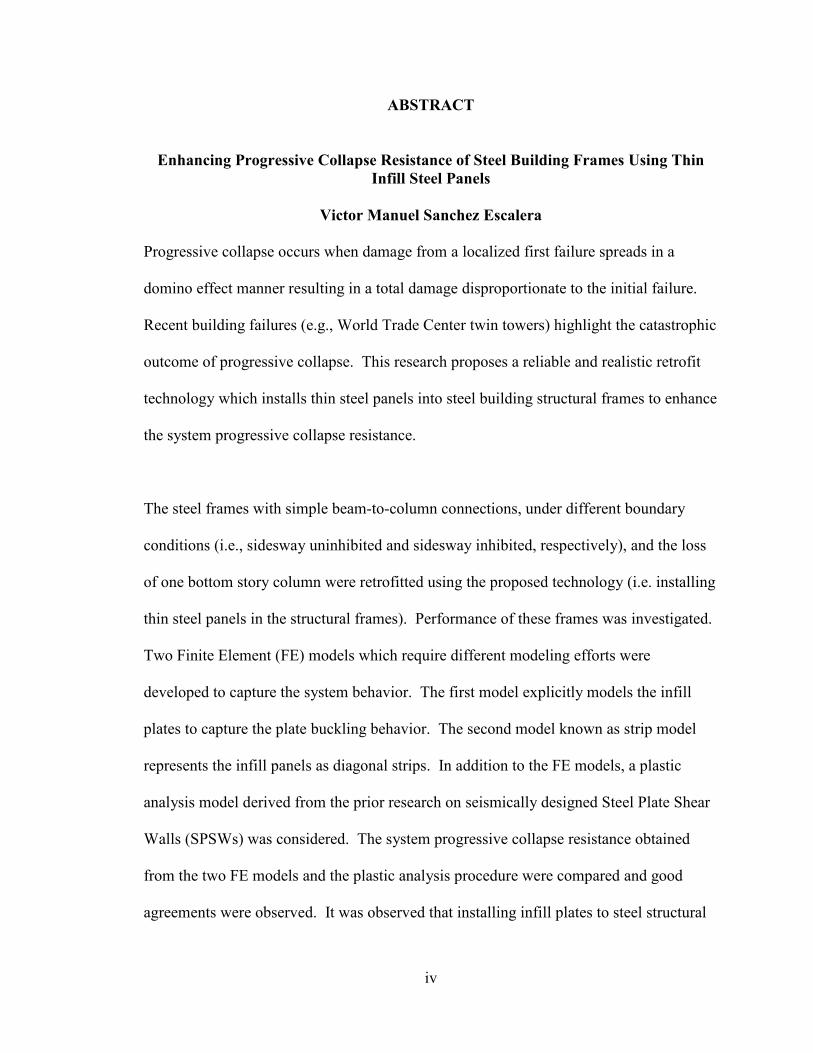
ABSTRACT
Enhancing Progressive Collapse Resistance of Steel Building Frames Using Thin
Infill Steel Panels
Victor Manuel Sanchez Escalera
Progressive collapse occurs when damage from a localized first failure spreads in a
domino effect manner resulting in a total damage disproportionate to the initial failure.
Recent building failures (e.g., World Trade Center twin towers) highlight the catastrophic
outcome of progressive collapse. This research proposes a reliable and realistic retrofit
technology which installs thin steel panels into steel building structural frames to enhance
the system progressive collapse resistance.
The steel frames with simple beam-to-column connections, under different boundary
conditions (i.e., sidesway uninhibited and sidesway inhibited, respectively), and the loss
of one bottom story column were retrofitted using the proposed technology (i.e. installing
thin steel panels in the structural frames). Performance of these frames was investigated.
Two Finite Element (FE) models which require different modeling efforts were
developed to capture the system behavior. The first model explicitly models the infill
plates to capture the plate buckling behavior. The second model known as strip model
represents the infill panels as diagonal strips. In addition to the FE models, a plastic
analysis model derived from the prior research on seismically designed Steel Plate Shear
Walls (SPSWs) was considered. The system progressive collapse resistance obtained
from the two FE models and the plastic analysis procedure were compared and good
agreements were observed. It was observed that installing infill plates to steel structural
v
frames can be an effective approach for enhancing the system progressive collapse
resistance.
Beyond the strength of the overall system, the Dynamic Increase Factor (DIF) which may
be used to amplify the static force on the system to better capture the dynamic nature of
progressive collapse demand was evaluated for the retrofitted system. Furthermore, the
demands including axial force, shear force and bending moment on individual frame
components (i.e., beams and columns) in the retrofitted system were quantified via the
nonlinear FE models and a simplified procedure based on free body diagrams (FBDs).
Finally, the impact of premature beam-to-column connection failures on the system
performance was investigated and it was observed that the retrofitted system is able to
provide stable resistance even when connection failures occur in all beams.

vi
ACKNOWLEDGEMENTS
I will like to express my sincere appreciation and gratitude to Dr. Bing Qu. His great
knowledge, enthusiasm and encouragement are invaluable. Without his guidance this
thesis would have been impossible.
Thanks to Professor Rakesh Goel and Dr. Juan Cepeda-Rizo for taking the time out of
their very busy schedules to serve on my thesis defense committee.
I am very grateful for the financial support through the California Central Coast Research
Partnership (C3RP) program sponsored by the Office of Naval Research.
Thank you to Maria Manzano, for the opportunity to work at the tutoring center and for
the scholarships and endless meals that she provided. Also, for the generous assistance
provided to other first generation college students.
Thanks to all the students and professors with whom I had interaction during my studies
at Cal Poly. Especially to fellow graduate students: Brad Stirling, Gary Guo and Paul
Gordon for the good times we spent together in the graduate lab.
I want to express gratitude to my family for all of their moral support. Although they
have minimum understanding of what exactly is taking me so long in school, they keep
providing their support and motivation. I want to especially thank my cousins Juan
Sanchez and Francisco Sanchez for all of their support and input on this thesis.
(Me gustaría agradecer a mi familia por todo su apoyo moral. Aunque, ellos no tienen la
mínima idea de que es lo que me está tomando tanto tiempo en la escuela, ellos me

vii
siguen apoyando y motivando. Especial agradecimiento para mis primos Juan y
Francisco Sánchez por todo su apoyo y comentarios en mi tesis.)
To my daughter Emma Denise Sanchez Flores for understanding that Papi had to leave
every week to keep working on the thesis. Thank you for understanding mi Corazon.
I want to show my appreciation to my fiancée, Carmen Hernandez, for her patience,
understanding and great support. Thank you mi Amor for not getting too upset when I
couldn’t talk to you when I was working on my thesis. I love you.
Overall, I am tremendously grateful with GOD for the opportunity to acquire a college
education and to complete this thesis.
viii
TABLE OF CONTENTS
LIST OF TABLES ............................................................................................................. xi
LIST OF FIGURES ........................................................................................................... xi
1 INTRODUCTION ...................................................................................................... 1
1.1 Scope .................................................................................................................... 2
1.2 Thesis Organization.............................................................................................. 3
2 LITERATURE REVIEW ........................................................................................... 5
2.1 Introduction .......................................................................................................... 5
2.2 Steel Plate Shear Walls (SPSWs) ......................................................................... 5
2.2.1 Wagner (1931) .............................................................................................. 7
2.2.2 Thorburn et al. (1983) ................................................................................... 7
2.2.3 Timler and Kulak (1983) .............................................................................. 9
2.2.4 Driver et al. (1997) ...................................................................................... 10
2.2.5 Behbahanifard et al. (2003) ......................................................................... 13
2.2.6 Berman and Bruneau (2003) ....................................................................... 14
2.2.7 Qu and Bruneau (2008) ............................................................................... 14
2.3 Progressive Collapse .......................................................................................... 15
2.3.1 Previous Progressive Collapse Cases.......................................................... 16
2.3.2 Code Provisions and Design Guidelines ..................................................... 19
2.3.3 Past Research on Enhancing Progressive Collapse Resistance .................. 21
2.4 Summary ............................................................................................................ 32
3 PLASTIC ANALYSIS OF THE PROPOSED SYSTEM ........................................ 33
3.1 Consideration of Initial Column Failure ............................................................ 33
3.2 Proposed System ................................................................................................ 34
3.3 System Behavior ................................................................................................ 36
3.3.1 Infill Panel – Tension Field Action ............................................................. 37
3.3.1.1 Equilibrium Method – Single Story Frame ......................................... 37
3.3.1.2 Kinematic Method – Single Story Frame ............................................ 46
3.3.1.3 Kinematic Method – Multistory Frame ............................................... 48
3.3.2 Boundary Frame Members - Catenary Actions .......................................... 49
3.3.2.1 Beam Catenary Action- Single Story Frame ....................................... 50
3.3.2.2 Beam Catenary Action-Multistory Frame ........................................... 56
3.3.3 Combination of Tension Fields and Catenary Actions ............................... 58
3.4 Summary ............................................................................................................ 58
4 DEVELOPMENT OF HIGH-FIDELITY ANALYTICAL MODELS .................... 59

ix
4.1 Introduction ........................................................................................................ 59
4.2 Demonstration Structure .................................................................................... 59
4.3 3D FE Model Using ABAQUS .......................................................................... 60
4.3.1.1 Parts ..................................................................................................... 62
4.3.1.2 Materials .............................................................................................. 62
4.3.1.3 Section ................................................................................................. 63
4.3.1.4 Profile .................................................................................................. 63
4.3.1.5 Step ...................................................................................................... 63
4.3.1.6 Constraints ........................................................................................... 64
4.3.1.7 Load ..................................................................................................... 65
4.3.1.8 Boundary Conditions ........................................................................... 65
4.3.1.9 Mesh .................................................................................................... 66
4.4 Strip Model using SAP2000 ............................................................................... 67
4.4.1 Parts............................................................................................................. 69
4.4.2 Restrains ...................................................................................................... 69
4.4.3 Materials ..................................................................................................... 69
4.4.4 Sections ....................................................................................................... 70
4.4.5 Plastic Hinges.............................................................................................. 70
4.4.6 Load ............................................................................................................ 71
4.5 Summary ............................................................................................................ 71
5 DISCUSSION AND COMPARISON OF RESULTS FROM DEVELOPED
ANALYTICAL MODELS ............................................................................................... 72
5.1 Introduction ........................................................................................................ 72
5.2 Considered Boundary Conditions ...................................................................... 72
5.3 Discussion and Comparison of Results .............................................................. 74
5.3.1 Boundary Condition #1 ............................................................................... 74
5.3.2 Boundary Condition #2 ............................................................................... 80
5.3.3 Boundary Condition #3 ............................................................................... 86
5.3.4 Boundary Condition #4 ............................................................................... 93
5.3.5 Boundary Condition #5 ............................................................................... 99
5.4 Summary .......................................................................................................... 106
6 PSEUDO-STATIC RESPONSE OF THE PROPOSED SYSTEM ....................... 107
6.1 Introduction ...................................................................................................... 107
6.2 Observations and Summary ............................................................................. 109
7 DEMANDS ON BOUNDARY FRAME MEMBERS ........................................... 116
x
7.1 Introduction ...................................................................................................... 116
7.2 Tension Field Action along Frame Members ................................................... 117
7.3 Demand on Beams ........................................................................................... 119
7.3.1 General FBDs of Beams ........................................................................... 120
7.3.2 Results from Different Boundary Conditions ........................................... 122
7.3.2.1 Boundary Condition #1 ..................................................................... 122
7.3.2.2 Boundary Condition #2 ..................................................................... 128
7.3.2.3 Boundary Condition #3 ..................................................................... 133
7.3.2.4 Boundary Condition #4 ..................................................................... 138
7.3.2.5 Boundary Condition #5 ..................................................................... 145
7.4 Demands on Columns ...................................................................................... 154
7.4.1 General FBDs of the Columns .................................................................. 154
7.4.2 Results from Different Boundary Conditions ........................................... 156
7.4.2.1 Boundary Condition #1 ..................................................................... 156
7.4.2.2 Boundary Condition #2 ..................................................................... 160
7.4.2.3 Boundary Condition #3 ..................................................................... 164
7.4.2.4 Boundary Condition #4 ..................................................................... 167
7.4.2.5 Boundary Condition #5 ..................................................................... 171
7.5 Summary .......................................................................................................... 174
8 IMPACT OF BEAM-TO-COLUMN CONNECTION FAILURE ON SYSTEM
BEHAVIOR .................................................................................................................... 176
8.1 Introduction ...................................................................................................... 176
8.2 Case Studies ..................................................................................................... 178
8.3 Summary .......................................................................................................... 189
9 SUMMARY, CONCLUSIONS, AND RECOMMENDATIONS FOR FUTURE
RESEARCH .................................................................................................................... 190
9.1 Summary and Conclusions ............................................................................... 190
9.2 Recommendations for Future Research ........................................................... 191
REFERENCES ............................................................................................................... 193
APPENDIX A – ALGORITHM USED TO DETERMINE THE PSEUDO-STATIC
RESPONSE..................................................................................................................... 196
xi
LIST OF TABLES
Table 8-1: Cases considered for system with beam-to-column failures ......................... 179
Table 8-2: Capacities of the systems with connection failures* ..................................... 187
LIST OF FIGURES
Figure 2-1 General SPSW configuration (Berman and Bruneau 2008) ............................. 6
Figure 2-2: Schematic of SPSW Strip Model (Thorburn et al. 1983) ................................ 8
Figure 2-3: FE Model Subjected to 2200 KN (Driver et al. 1997) ................................... 11
Figure 2-4: Strip Model of Test Specimen (Driver et al. 1998)........................................ 12
Figure 2-5: Finite Element Model (Behbahanifard et al. 2003)........................................ 13
Figure 2-6: Tension Field Action of the FE Model (Qu and Bruneau 2008) ................... 15
Figure 2-7: Ronan Point March 1968 (Wearne 2000) ...................................................... 17
Figure 2-8: Alfred P. Murrah Federal Building (Crowder 2004) ..................................... 18
Figure 2-9: collision of flight UA175 Boeing 767 jet with south tower of WTC
(Level3.com Sep 20, 2001) ............................................................................................... 19
Figure 2-10: Plan view of the tested specimen with catenary cables
(Astaneh-Asl 2007) ........................................................................................................... 22
Figure 2-11: Test Results (Astaneh-Asl 2007) ................................................................. 23
Figure 2-12: Specimen and the retrofit cable end anchorage (Astaneh-Asl, 2007) .......... 24
Figure 2-13: Column removal strategy (DoD UFC 2009) ................................................ 25
Figure 2-14: Test Specimen (Astaneh-Asl et al. 2001) ..................................................... 26
Figure 2-15: Beam-to-column connections (left) beam-to-girder connections (right)
(Astaneh-Asl et al. 2001) .................................................................................................. 27
Figure 2-16: Specimen after testing (Astaneh-Asl at al. 2001) ........................................ 28
Figure 2-17: Original design of fin plate joins (Li 2009) ................................................. 29
Figure 2-18: Retrofitting scheme 1 (J.L. Li 2009) ............................................................ 30
Figure 2-19: Retrofitting scheme 2 (Li 2009) ................................................................... 30
Figure 3-1: Frame before and after removal a column (Astaneh-Asl 2007) ..................... 34
Figure 3-2: Proposed system ............................................................................................. 35
Figure 3-3: Single plate field tension action of SPSW and proposed system ................... 35
Figure 3-4: Tension field actions in multistory SPSWs and the proposed system .......... 36
Figure 3-5: Strip model of a single SPSW with simple beam-to-column connection ...... 38
Figure 3-6: Zone 1 FBD - Top beam and right column .................................................... 38
Figure 3-7: Zone 1 FBD - Right column .......................................................................... 39
Figure 3-8: Zone 2 FBD - Top beam and right column .................................................... 41
Figure 3-9: Zone 2 FBD - Right column .......................................................................... 41
Figure 3-10: Zone 3 FBD - Bottom beam ......................................................................... 43
Figure 3-11 : Kinematic collapse mechanism single story tension field action ............... 46
Figure 3-12: Tension field distributions in a multistory frame subjected to sudden
column loss ....................................................................................................................... 48
Figure 3-13: The three-hinge beam by Timoshenko (1955) ............................................. 50
xii
Figure 3-14: Force-displacement relationship for a three-hinge beam Astaneh-Asl
(2007) ................................................................................................................................ 52
Figure 3-15: Force-displacement relationship for a three hinge beam beyond its yield
point (Astaneh-Asl 2007) .................................................................................................. 54
Figure 3-16: Three-hinge girder with end supports axially semi-rigid
(Asteneh-Asl, 2007) .......................................................................................................... 55
Figure 3-17: Vertical load resistance vs. beam cross-sectional area ................................ 56
Figure 3-18: Catenary action of a multistory frame under column loss ........................... 57
Figure 4-1: Demonstration steel frame structure .............................................................. 60
Figure 4-2: Model development diagram ......................................................................... 61
Figure 4-3: SAP2000 Strip Model .................................................................................... 68
Figure 4-4: Plastic Hinge Parameters ............................................................................... 70
Figure 5-1: Considered boundary conditions .................................................................... 73
Figure 5-2: Buckling modes for the retrofitted system under Boundary Condition #1
(Results from ABAQUS) .................................................................................................. 75
Figure 5-3: Post buckling behavior of the retrofitted system and deflection of the
original frame under Boundary Condition #1 (Results from ABAQUS) ......................... 76
Figure 5-4: Deformed shape of the retrofitted system and the original frame under
Boundary Condition #1 (Results from SAP2000) ............................................................ 77
Figure 5-5: Vertical load resistance of the retrofitted system and the original frame
under Boundary Condition #1 (Results from ABAQUS) ................................................. 78
Figure 5-6: Vertical load resistance of the retrofitted system and the original frame
under Boundary Condition #1 (Results from SAP2000) .................................................. 78
Figure 5-7: Vertical load resistance of the retrofitted system and the original frame
under Boundary Condition #1 (Results from Plastic Analysis) ........................................ 79
Figure 5-8: Comparison of vertical load resistance of the original frame under
Boundary Condition #1 ..................................................................................................... 79
Figure 5-9 Comparison of vertical load resistance of the infill panels alone under
Boundary Condition #1 ..................................................................................................... 80
Figure 5-10: Comparison of vertical load resistance of the retrofitted system under
Boundary Condition #1 ..................................................................................................... 80
Figure 5-11: Buckling modes for the retrofitted system under Boundary Condition #2
(Results from ABAQUS) .................................................................................................. 81
Figure 5-12: Post buckling behavior of the retrofitted system and deflection of the
original frame under Boundary Condition #2 (Results from ABAQUS) ......................... 82
Figure 5-13: Deformed shape of the retrofitted system and the original frame under
Boundary Condition #2 (Results from SAP2000) ............................................................ 83
Figure 5-14: Vertical load resistance of the retrofitted system and the original frame
under Boundary Condition #2 (Results from ABAQUS) ................................................. 84
Figure 5-15: Vertical load resistance of the retrofitted system and the original frame
under Boundary Condition #2 (Results from SAP2000) .................................................. 84
Figure 5-16: Vertical load resistance of the retrofitted system and the original frame
under Boundary Condition #2 (Results from Plastic Analysis) ........................................ 85
Figure 5-17: Comparison of vertical load resistance of the original frame under
Boundary Condition #2 ..................................................................................................... 85

xiii
Figure 5-18 Comparison of vertical load resistance of the infill panels alone under
Boundary Condition #2 ..................................................................................................... 86
Figure 5-19: Comparison of vertical load resistance of the retrofitted system under
Boundary Condition #2 ..................................................................................................... 86
Figure 5-20: Buckling modes for the retrofitted system under Boundary Condition #3
(Results from ABAQUS) .................................................................................................. 87
Figure 5-21: Post buckling behavior of the retrofitted system and deflection of the
original frame under Boundary Condition #3 (Results from ABAQUS) ......................... 88
Figure 5-22: Deformed shape of the retrofitted system and the original frame under
Boundary Condition #3 (Results from SAP2000) ............................................................ 89
Figure 5-23: Vertical load resistance of the retrofitted system and the original frame
under Boundary Condition #3 (Results from ABAQUS) ................................................. 90
Figure 5-24: Vertical load resistance of the retrofitted system and the original frame
under Boundary Condition #3 (Results from SAP2000) .................................................. 90
Figure 5-25: Vertical load resistance of the retrofitted system and the original frame
under Boundary Condition #3 (Results from Plastic Analysis) ........................................ 91
Figure 5-26: Comparison of vertical load resistance of the original frame under
Boundary Condition #3 ..................................................................................................... 91
Figure 5-27: Comparison of vertical load resistance of the infill panels alone under
Boundary Condition #3 ..................................................................................................... 92
Figure 5-28: Comparison of vertical load resistance of the retrofitted system under
Boundary Condition #3 ..................................................................................................... 92
Figure 5-29: Buckling modes for the retrofitted system under Boundary Condition #4
(Results from ABAQUS) .................................................................................................. 93
Figure 5-30: Post buckling behavior of the retrofitted system and deflection of the
original frame under Boundary Condition #4 (Results from ABAQUS) ......................... 94
Figure 5-31 shows the deflections of the retrofitted system and the original system
modeled in SAP 2000. ...................................................................................................... 95
Figure 5-32: Deformed shape of the retrofitted system and the original frame under
Boundary Condition #4 (Results from SAP2000) ............................................................ 95
Figure 5-33: Vertical load resistance of the retrofitted system and the original frame
under Boundary Condition #4 (Results from ABAQUS) ................................................. 96
Figure 5-34: Vertical load resistance of the retrofitted system and the original frame
under Boundary Condition #4 (Results from SAP2000) .................................................. 96
Figure 5-35: Vertical load resistance of the retrofitted system and the original frame
under Boundary Condition #4 (Results from Plastic Analysis)) ...................................... 97
Figure 5-36: Comparison of vertical load resistance of the original frame under
Boundary Condition #4 ..................................................................................................... 97
Figure 5-37: Comparison of vertical load resistance of the infill panels alone under
Boundary Condition #4 ..................................................................................................... 98
Figure 5-38: Comparison of vertical load resistance of the retrofitted system under
Boundary Condition #4 ..................................................................................................... 98
Figure 5-39: Column base reaction of the retrofitted system under Boundary
Condition #4...................................................................................................................... 99
Figure 5-40: Buckling modes for the retrofitted system under Boundary
Condition #5 (Results from ABAQUS) .......................................................................... 100

xiv
Figure 5-41: Post buckling behavior of the retrofitted system and deflection of the
original frame under Boundary Condition #5 (Results from ABAQUS) ....................... 101
Figure 5-42: Deformed shape of the retrofitted system and the original frame
under Boundary Condition #5 (Results from SAP2000) ................................................ 102
Figure 5-43: Vertical load resistance of the retrofitted system and the original frame
under Boundary Condition #5 (Results from ABAQUS) ............................................... 103
Figure 5-44: Vertical load resistance of the retrofitted system and the original frame
under Boundary Condition #5 (Results from SAP2000) ................................................ 103
Figure 5-45: Vertical load resistance of the retrofitted system and the original frame
under Boundary Condition #5 (Results from Plastic Analysis) ...................................... 104
Figure 5-46: Comparison of vertical load resistance of the original frame under
Boundary Condition #5 ................................................................................................... 104
Figure 5-47: Comparison of vertical load resistance of the infill panels alone under
Boundary Condition #5 ................................................................................................... 105
Figure 5-48: Comparison of vertical load resistance of the retrofitted system under
Boundary Condition #5 ................................................................................................... 105
Figure 5-49: Column base reactions of the retrofitted system under Boundary
Condition #5.................................................................................................................... 106
Figure 6-1: Modified performance for the system under Boundary Condition #1 ......... 111
Figure 6-2: Dynamic load amplification factor for the system under Boundary
Condition #1.................................................................................................................... 111
Figure 6-3: Modified performance for the system under Boundary Condition #2 ......... 112
Figure 6-4: Dynamic load amplification factor for the system under Boundary
Condition #2.................................................................................................................... 112
Figure 6-5: Modified performance for the system under Boundary Condition #3 ......... 113
Figure 6-6: Dynamic load amplification factor for the system under Boundary
Condition #3.................................................................................................................... 113
Figure 6-7: Modified performance for the system under Boundary Condition #4 ......... 114
Figure 6-8: Dynamic load amplification factor for the system under Boundary
Condition #4.................................................................................................................... 114
Figure 6-9: Modified performance for the system under Boundary Condition #5 ......... 115
Figure 6-10: Dynamic load amplification factor for the system under Boundary
Condition #5.................................................................................................................... 115
Figure 7-1: Tension field actions in a structural Frame .................................................. 117
Figure 7-2: Tension Field actions along columns and beams ......................................... 118
Figure 7-3: General FBDs of beams (a) Sidesway uninhibited (b) Sidesway inhibited . 120
Figure 7-4: Axial, shear, and moment diagrams for the top anchor beam under
Boundary Condition #1 ................................................................................................... 124
Figure 7-5: Axial, shear, and moment diagrams for the bottom anchor beam under
Boundary Condition #1 ................................................................................................... 125
Figure 7-6: Axial, shear, and moment diagrams for the intermediate beam under
Boundary Condition #1 ................................................................................................... 127
Figure 7-7: Axial, shear, and moment diagrams for the top anchor beam under
Boundary Condition #2 ................................................................................................... 129
Figure 7-8: Axial, shear, and moment diagrams for the bottom anchor beam under
Boundary Condition #2 ................................................................................................... 130

xv
Figure 7-9: Axial, shear, and moment diagrams for the intermediate anchor beams
under Boundary Condition #2 ......................................................................................... 132
Figure 7-10: Axial, shear, and moment diagrams for the top anchor beam under
Boundary Condition #3 ................................................................................................... 134
Figure 7-11: Axial, shear, and moment diagrams for the bottom anchor beam under
Boundary Condition #3 ................................................................................................... 135
Figure 7-12: Axial, shear, and moment diagrams for the intermediate beams under
Boundary Condition #3 ................................................................................................... 137
Figure 7-13: Axial, shear, and moment diagrams for the top right anchor beam under
Boundary Condition #4 ................................................................................................... 139
Figure 7-14: Axial, shear, and moment diagrams for the bottom right anchor beam
under Boundary Condition #4 ......................................................................................... 140
Figure 7-15: Axial, shear, and moment diagrams for the top left anchor beam under
Boundary Condition #4 ................................................................................................... 141
Figure 7-16: Axial, shear, and moment diagrams for the bottom left anchor beam
under Boundary Condition #4 ......................................................................................... 142
Figure 7-17: Axial, shear, and moment diagrams for the intermediate beams under
Boundary Condition #4 ................................................................................................... 144
Figure 7-18: Axial, shear, and moment diagrams for the top right anchor beam
under Boundary Condition #5 ......................................................................................... 146
Figure 7-19: Axial, shear, and moment diagrams for the bottom right anchor beam
under Boundary Condition #5 ......................................................................................... 147
Figure 7-20: Axial, shear, and moment diagrams for the top left anchor beam under
Boundary Condition #5 ................................................................................................... 149
Figure 7-21: Axial, shear, and moment diagrams for the bottom left anchor beam
under Boundary Condition #5 ......................................................................................... 150
Figure 7-22: Axial, shear, and moment diagrams for the right intermediate beams
under Boundary Condition #5 ......................................................................................... 152
Figure 7-23: Axial, shear, and moment diagrams for the top left intermediate beam
under Boundary Condition #5 ......................................................................................... 153
Figure 7-24: General FBDs of columns: (a) Sidesway uninhibited (b) Sidesway
inhibited .......................................................................................................................... 154
Figure 7-25: Axial, shear, and moment diagrams for the right column under
Boundary Condition #1 ................................................................................................... 157
Figure 7-26: Axial, shear, and moment diagrams for the middle column under
Boundary Condition #1 ................................................................................................... 159
Figure 7-27: Axial, shear, and moment diagrams for the right column due under
Boundary Condition #2 ................................................................................................... 161
Figure 7-28: Axial, shear, and moment diagrams for the left column under
Boundary Condition #2 ................................................................................................... 162
Figure 7-29: Axial, shear, and moment diagrams for the middle column under
Boundary Condition #2 ................................................................................................... 163
Figure 7-30: Axial, shear, and moment diagrams for the right column under
Boundary Condition #3 ................................................................................................... 165
Figure 7-31: Axial, shear, and moment diagrams for the middle column under
Boundary Condition #3 ................................................................................................... 166

xvi
Figure 7-32: Axial, shear, and moment diagrams for the left column under
Boundary Condition #4 ................................................................................................... 168
Figure 7-33: Axial, shear, and moment diagrams for the middle beam under
Boundary Condition #4 ................................................................................................... 169
Figure 7-34: Axial, shear, and moment diagrams for the right column under
Boundary Condition #4 ................................................................................................... 170
Figure 7-35: Axial, shear, and moment diagrams for the left column under
Boundary Condition #5 ................................................................................................... 172
Figure 7-36: Axial, shear, and moment diagrams for the middle column under
Boundary Condition #5 ................................................................................................... 173
Figure 7-37: Axial, shear, and moment diagrams for the right column under
Boundary Condition #5 ................................................................................................... 174
Figure 8-1: Tension field action distribution in the frame under Boundary
Condition #3 and Case A connection failures................................................................. 181
Figure 8-2: Vertical resistance of the system under Boundary Condition #3 and
Case A connection failures ............................................................................................. 182
Figure 8-3: Tension field action distribution in the frame under Boundary
Condition #3 and Case B connection failures ................................................................. 183
Figure 8-4: Vertical resistance of the system under Boundary Condition #3 and
Case B connection failures .............................................................................................. 184
Figure 8-5: Tension field action distribution in the frame under Boundary
Condition #3 and Case C connection failures ................................................................. 185
Figure 8-6: Vertical resistance of the system under Boundary Condition #3 and
Case C connection failures .............................................................................................. 186
Figure 8-7: Tension field action distribution in the frame under Boundary
Condition #3 and Case D connection failures................................................................. 188
Figure 8-8: Vertical resistance of the system under Boundary Condition #3 and
Case D connection failures ............................................................................................. 189
1
1 INTRODUCTION
Progressive collapse occurs when the damage from a localized first failure spreads in a
domino effect manner resulting in a total damage disproportionate to the initial failure. In
Section C1.4 General Structural Integrity of the American Society of Civil Engineers
(ASCE) -7 Standard: Minimum Design Loads for Buildings and Other Structures (ASCE
2005), progressive collapse is defined as “the spread of an initial local failure from
element to element resulting, eventually, in the collapse of an entire structure or a
disproportionately large part of it". In addition, ASCE -7 defines the resistance to
progressive collapse as “the ability of a structure to accommodate, with only local failure,
the notional removal of any single structural member".
Progressive collapse has been observed as one of the most catastrophic failure modes of
building structures and it may be caused by different excitations (e.g. fire, blast, collision,
and foundation failure) in the structures (in particular at the bottom story of the structure).
In an event that a building structure is subjected to abnormal loading, in addition to
bearing the localized failure caused by the excitation, the structure is subjected to its
service loads (e.g. wind and gravity). Depending on the magnitude of the unexpected
loading and the structure's ability to withstand local damage, the damaged structure
would either continue to support the service loads or it would progressively collapse. If
the structure has adequate continuity, ductility, and redundancy to resists the spread of
damage, only localized failure would occur; otherwise progressive collapse develops. In
most cases where progressive collapse develops, the majority of the fatal casualties are
2
attributed to the structural damage caused during progressive collapse rather than to the
initial abnormal load (Astaneh-Asl 2007).
This thesis investigates the behavior of a system developed for prevention of progressive
collapse of steel building frames. In this system (referred to herein as “the proposed
system”), the unstiffened thin infill steel panels are installed in the building structural
frame to increase its continuity and redundancy. In a scenario of initial column failures
which may likely trigger the system progress collapse, these infill panels are allowed to
buckle in shear and then develop the diagonal tension field actions. Such tension field
actions will bridge over the missing column, transfer the load from the damaged column
to the adjacent columns, and consequently prevent the development of progressive
collapse.
1.1 Scope
For the proposed system, this thesis focused on behavior modeling and system
performance assessment. A total of three models were developed. Building on the prior
research outcome on plastic analysis of seismically designed steel plate shear walls
(SPSWs), the first model was developed based on the classic plastic analysis framework.
The second and third models were developed using the Finite Element (FE) technology.
The second model is a 3D FE model which explicitly models the infill plates using shell
element to capture the plate buckling behavior. The third model is a simplified 2D FE
model which represents the infill panels as diagonal strips. With the developed analytical
models, behavior of the proposed system including ultimate strength and dynamic

3
amplification effects were evaluated followed by development and validation of the free
body diagrams (FBDs) for estimating the shear force, bending moment and axial force in
the beams and columns of the system. Moreover, the impact of premature beam-to-
column connection fractures on performance of the proposed system was investigated.
1.2 Thesis Organization
This thesis includes a total of 9 chapters to address the key issues within the scope
presented in the prior section.
Chapter 2 presents an overview of past research related to analytical modeling of SPSWs.
In addition, prior investigations on progressive collapse of building structures are
included.
Chapter 3 describes the proposed system and its behavior under the column removal
scenario followed by derivation of a plastic analysis model for quantification of the
progressive collapse resistance of the proposed system.
Chapter 4 presents the development of two analytical models: a 3D finite element model
and a simplified 2D model known as strip model for validating the analytical models
derived in Chapter 3.
Chapter 5 compares results obtained from the three models described in Chapters 3 and 4
together with a discussion of the effectiveness of the proposed system.
4
Chapter 6 investigate the dynamic amplification effects and determines the factors which
capture the dynamic nature of progressive loading and can be used to modify the
performance of the proposed system obtained from the nonlinear static analyses.
Chapter 7 analyzes the demand on the boundary members (i.e. beams and columns). A
procedure developed based on FBDs is presented and validated by the results from the
nonlinear FE analysis.
Chapter 8 assesses the performance and robustness of the proposed system under the
premature beam-to-column connection failures.
Chapter 9 presents summary, conclusions, and recommendations for future research on
the proposed system.
5
2 LITERATURE REVIEW
2.1 Introduction
The system considered in this thesis consists of thin infill steel panels installed in steel
building frames. When an extreme event which causes the loss of a bottom story column
occurs, the infill panels will buckle in shear and then develop diagonal tension field
actions in the building structural frame which resists and transfers the gravity load on the
building frame, preventing progressive collapse development. Such a system is proposed
here based on the inspiration from SPSWs, a relatively new lateral force resisting system
in seismic design community. Therefore, to have a better understanding of the overall
behavior of the proposed system, an extensive literature review on SPSWs is presented in
Section 2.2 followed by a review on recent research on progressive collapse phenomenon
and different retrofit strategies to enhance progressive collapse resistance of building
structures in Section 2.3.
2.2 Steel Plate Shear Walls (SPSWs)
A conventional SPSW consists of beams, columns and infill panels as shown in Figure
2-1. These beams and columns are also known as horizontal boundary elements (HBEs)
and vertical boundary elements (VBEs), respectively. The infill panel is typically a thin
steel sheet which is anchored to the surrounding boundary frame elements. SPSWs have
been used as lateral force resisting systems in seismic design practice in many countries
such as Japan, Taiwan, Canada and the United States.

6
Figure 2-1 General SPSW configuration (Berman and Bruneau 2008)
Investigation on the SPSW infill panel performance was initiated from its application in
aerospace engineering. To date, significant research efforts, both analytical and
experimental, have been made to achieve a better understand of the panel post buckling
behavior. The following literature review is presented in a chronological order to capture
the evolvement of the infill panels from an aerospace application to the current seismic
design application. Since this thesis focuses on analytical work, the literature review was
conducted with emphasis on past analytical and simulation work.

7
2.2.1 Wagner (1931)
While performing investigations for the National Advisory Committee for Aeronautics,
Wagner showed that the thin aluminum shear panels used in aircrafts and supported by
stiff boundary members develop a diagonal tension field after buckling. From his
analysis, Wagner developed what he called the “pure tension field” theory which proved
that the capacity of a thin plate attached to a relative stiffer boundary frame depends on
the tension field action. These results ended the misconception that shear panels would
provide all of their strength up to the buckling stage. In contrast, Wagner demonstrated
that the buckling of these plates is not the limit state for determination of their shear
capacity. Consequently, the load resistance mechanism changes from in-plane shear
buckling to diagonal tension yielding.
2.2.2 Thorburn et al. (1983)
Thorburn et al. developed two models that would consider the behavior of thin
unstiffened steel plates in SPSWs. These models focused on determination of the
ultimate shear strength of SPSWs and the shear resistance of the walls prior to buckling
was not addressed. Wagner’s (1931) idea of pure tension field action was implemented
on these models. These models are commonly known as the strip model and the
equivalent brace model.
In the strip model the infill panel was modeled by a series of pin-ended inclined tension
members. The strips were oriented parallel to the direction of the tension fields and were
8
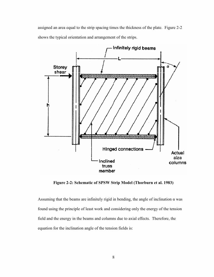
assigned an area equal to the strip spacing times the thickness of the plate. Figure 2-2
shows the typical orientation and arrangement of the strips.
Figure 2-2: Schematic of SPSW Strip Model (Thorburn et al. 1983)
Assuming that the beams are infinitely rigid in bending, the angle of inclination α was
found using the principle of least work and considering only the energy of the tension
field and the energy in the beams and columns due to axial effects. Therefore, the
equation for the inclination angle of the tension fields is:

9
4
12
tan ( )
1
c
b
L t
A
H t
A
α
⋅+
⋅=
⋅+
(2-1)
where α = the angle of inclination of the tension field,
L = the bay width
t = is the infill plate thickness
Ab = cross-section area of the beam
Ac = cross-section area of the column
From their analytical studies, Thorburn et al. concluded that 10 strips per panel would be
sufficient to accurately model the infill plate behavior.
In the equivalent brace model the investigators modeled the infill panel with a single
equivalent diagonal truss element at each floor. This element had the same story
stiffness. This model is practical to determine the story stiffness.
2.2.3 Timler and Kulak (1983)
In 1983, Timler and Kulak performed laboratory testing of a full scale SPSW to verify
the model derived by Thorburn et al (1983). The test specimen was composed of two 5
mm thick infill panels of 3750 mm bay width and 2500 mm story height. For the VBEs
and HBEs, W18X97 and W12X87 were used, respectively. The specimen was subjected
to quasi-static reverse cyclic loading to a drift of 6.25 mm, and then it was loaded
monotonically to failure.

10
Timler and Kulak concluded that Thornborn’s equation did not include the effects of
column flexibility and they revised equation (2-1) to be:
4
3
12
tan ( )1
1360
c
b c
L t
A
HH t
A I L
α
⋅+
⋅=
+ ⋅ ⋅ + ⋅ ⋅
(2-2)
where Ic = the moment of inertia of the column and all the other terms have been
previously defined.
2.2.4 Driver et al. (1997)
Driver et al. developed a finite element (FE) model and a strip model to simulate the
behavior of a four story SPSW specimen. For the FE model, Driver et al. used the 1994
edition of the finite element software ABAQUS. The infill panels were modeled using
the eight-node quadratic shell element (S8R5), while the beams and columns were
modeled using the three-node quadratic beam element (B32). The infill panels were
connected to the boundary frame directly, instead of modeling the fish plate which was
used in the test specimen. This method to model the connection between the plate and
the boundary frame was proved to be adequate. An elastic-perfectly plastic bilinear
constitutive stress-strain relationship was applied to represent the material properties.
The model was restrained against out-of-plane displacement. The initial imperfection of
10 mm was assigned to the first buckling mode of the infill panel. Figure 2-3 shows the
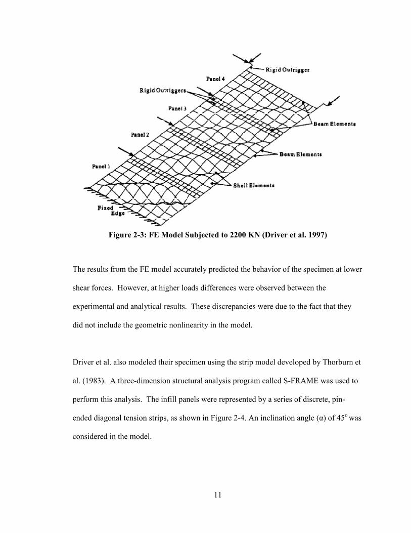
deformed model subject to a load of 2200 KN.
11
Figure 2-3: FE Model Subjected to 2200 KN (Driver et al. 1997)
The results from the FE model accurately predicted the behavior of the specimen at lower
shear forces. However, at higher loads differences were observed between the
experimental and analytical results. These discrepancies were due to the fact that they
did not include the geometric nonlinearity in the model.
Driver et al. also modeled their specimen using the strip model developed by Thorburn et
al. (1983). A three-dimension structural analysis program called S-FRAME was used to
perform this analysis. The infill panels were represented by a series of discrete, pin-
ended diagonal tension strips, as shown in Figure 2-4. An inclination angle (α) of 45o
was
considered in the model.

12
Figure 2-4: Strip Model of Test Specimen (Driver et al. 1998)
After loading began and the strips started yielding, they were subsequently removed from
the model and replaced by their equivalent yielding force. Plastic hinges were placed on
the surrounding frame members to simulate softening. Reasonable results were obtained
from the model for the behavior of each panel and for the entire wall. Nonetheless, the
model underestimated the elastic stiffness of the test specimen.
13
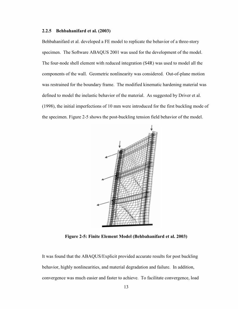
2.2.5 Behbahanifard et al. (2003)
Behbahanifard et al. developed a FE model to replicate the behavior of a three-story
specimen. The Software ABAQUS 2001 was used for the development of the model.
The four-node shell element with reduced integration (S4R) was used to model all the
components of the wall. Geometric nonlinearity was considered. Out-of-plane motion
was restrained for the boundary frame. The modified kinematic hardening material was
defined to model the inelastic behavior of the material. As suggested by Driver et al.
(1998), the initial imperfections of 10 mm were introduced for the first buckling mode of
the specimen. Figure 2-5 shows the post-buckling tension field behavior of the model.
Figure 2-5: Finite Element Model (Behbahanifard et al. 2003)
It was found that the ABAQUS/Explicit provided accurate results for post buckling
behavior, highly nonlinearities, and material degradation and failure. In addition,
convergence was much easier and faster to achieve. To facilitate convergence, load
14
increments of less than 10-5
were applied to the model. Good agreements were observed
between the results of the FE model and the test specimen.
2.2.6 Berman and Bruneau (2003)
Based on the strip model developed by Thorburn et al. (1983), Berman and Bruneau used
plastic analysis to determine the ultimate strength of SPSWs. Analytical models were
derived for single story and multistory SPSWs with either simple or rigid beam-to-
column connections.
Using both equilibrium and kinematic methods of plastic analysis, it was found that the
derived equations capture the ultimate strength of SPSWs. The results were compared
with other experimentally obtained results and agreement was observed. In addition, the
results were identical to that provided by the CAN/CSA S16-01 which is the procedure
used for calculating the shear resistance of a SPSW.
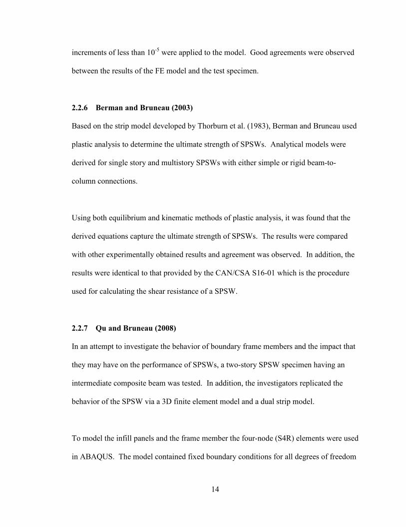
2.2.7 Qu and Bruneau (2008)
In an attempt to investigate the behavior of boundary frame members and the impact that
they may have on the performance of SPSWs, a two-story SPSW specimen having an
intermediate composite beam was tested. In addition, the investigators replicated the
behavior of the SPSW via a 3D finite element model and a dual strip model.
To model the infill panels and the frame member the four-node (S4R) elements were used
in ABAQUS. The model contained fixed boundary conditions for all degrees of freedom
15
of the nodes at the base of the SPSW. Out-of-plane displacements on the floor levels
were not allowed in the model. The model was subjected to eigenvalue buckling analysis
to determine the buckling modes of the infill panels. The obtained buckling modes were
used to introduce the initial imperfections of the infill panels. The model was then
subjected to monotonic pushover analysis. The behavior of the model can be observed in
Figure 2-6.
Figure 2-6: Tension Field Action of the FE Model (Qu and Bruneau 2008)
Both the strip model and the FE model yielded excellent correlation with the
experimental results. It was conclude that the modeling assumptions and model
development procedure utilized in the investigation are appropriate for modeling other
SPSWs.
2.3 Progressive Collapse
As mentioned earlier, ASCE-7 (ASCE 2005) defines progressive collapse as “the spread
of an initial local failure from element to element resulting, eventually, in the collapse of
an entire structure or a disproportionately large part of it". The standard further states
16
that buildings should be designed, “to sustained local damage with the structural system
as a whole remaining stable and not being damaged to an extent disproportionate to the
original local damage”. In other words, progressive collapse occurs when damage from a
localized first failure spreads in a domino effect manner resulting in a total damage
disproportionate to the initial failure. It has been observed as one of the most
catastrophic failure modes of building structures and it may be caused by different
excitations (e.g. fire, blast, collision, during and foundation failure). In fact, based on the
data from prior progressive collapse cases, most of the fatal casualties are attributed to
the damage caused by progressive collapse rather than to the unpredicted excitations.
2.3.1 Previous Progressive Collapse Cases
The Ronan Point disaster in March of 1968 triggered the consideration of progressive
collapse in design codes. The Ronan Point was a 22-story apartment complex designed
with precast-concrete load-bearing panels in Canning Town, England. A gas explosion in
the 18th floor blew out one wall which led to the collapse of the whole corner of the
building as shown in Figure 2-7. Due to insufficient progressive collapse resistance, all
the floors above and below the 18th
floor failed and collapsed one after the other in a
progressive manner. This disastrous event initiated significant research efforts on
investigating the progressive collapse behavior of building structures and it was
envisioned that better continuity and ductility, thus enhanced progressive collapse
resistance, might have had reduced the amount of damage (ASCE/SEI 7-2005).

17
Figure 2-7: Ronan Point March 1968 (Wearne 2000)
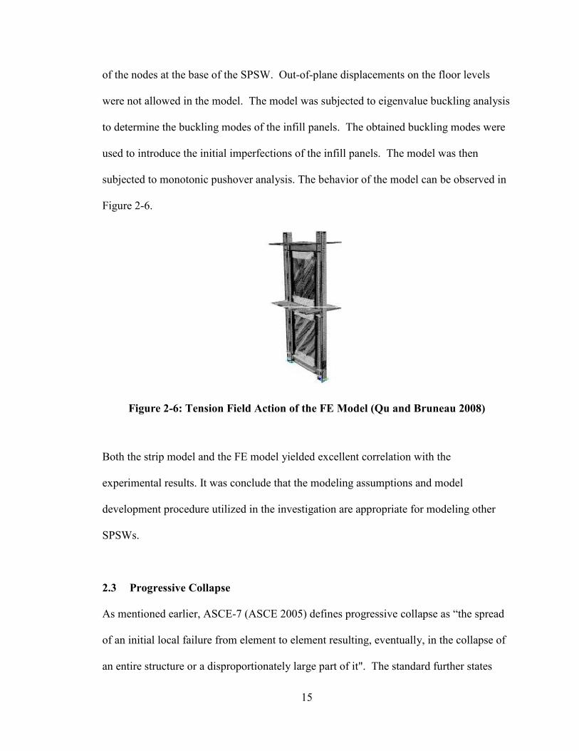
In a more recent well planned terrorist attack on April 19, 1995 in the US, a truck
containing approximately 4,000 lb of fertilizer-based explosive (ANFO) exploded outside
the ninth story Alfred P. Murrah Federal Building. The blast shockwave disintegrated
one of the 20x36 in. concrete perimeter columns and also caused brittle failure of two
others (ASCE/SEI 7-2005). Approximately 70 percent of the building experienced
dramatic collapse as shown in Figure 2-8. A total of 168 people died and many of those
deaths were due to progressive collapse. If a better system that could have enhanced the
18
progressive collapse resistance of this structure had been implemented, most of those
lives could have been saved (ASCE/SEI 7-2005).
Figure 2-8: Alfred P. Murrah Federal Building (Crowder 2004)
On September 11, 2001, the twin towers of the World Trade Center (WTC) in New York
City collapsed as the result of a terrorist attack. Two commercial airliners that had
departed from Boston’s Logan Airport were hijacked and flown into the two 110-story
towers. Some technical debates rose regarding the actual cause of the localized failure;
nonetheless a combination of the structural damages respectively from the impact and
fires resulted in progressive collapse and consequently total structural collapse of both
towers. A total of 2,270 people lost their lives at the WTC site due to the building
collapse (FEMA 2002).

19
Figure 2-9: collision of flight UA175 Boeing 767 jet with south tower of WTC
(Level3.com Sep 20, 2001)
2.3.2 Code Provisions and Design Guidelines
The ASCE standard 7, minimum Design loads for building and other structures
(ASCE/SEI 7-2005) provides an intensive and comprehensive building performance
statement in chapter C1. Section 1.4: General Structural Integrity. This commentary
addresses the quality of general structural integrity and provides two methods to address
the issue, namely direct design and indirect design. Direct design considers explicitly the
resistance to progressive collapse during the design process through either (ASCE/SEI 7-
2005):
1. Alternate Path Method- A method that allows local failure to occur, but seeks
to provide alternate load paths so that the damage is absorbed and major
collapse is avoided.
2. Specific Local Resistance Method- A method that seeks to provide sufficient
strength to resist failure from accidents or misuse.

20
The indirect design method considers the resistance to progressive collapse during the
design process through the provision of minimum levels of strength, continuity, and
ductility.
The Precast Concrete Institute (PCI) and the American Concrete Institute (ACI) also
provide recommendations and design guidelines to preserve structural integrity. The PCI
was the first American institutions to provide such guidelines in 1976 (Cleland 2007),
mainly because of the lack of redundancy in precast concrete structures. These guidelines
were added to the ACI in 1995. ACI extended these design recommendations to cast-in-
place concrete structures to enhance structural integrity via detailing requirements. These
new detailing requirement ensures that the structure would be able to redistribute load
from failed members enhancing structural collapse resistance. In addition, these detailing
requirements ensure tensile and moment reversal capacities and an overall increase in
ductility.
In an attempt to reduce the potential of progressive collapse for new and existing
facilities that experience localized structural damage through unforeseeable events, the
Unified Facilities Criteria (UFC) provides design requirements (DoD 2009). These
requirements were developed, independently, by the General Service Administration
(GSA) and by the Department of Defense (DoD) in 2003, in an attempt to protect
governmental and military facilities from potential progressive collapse caused by
terrorist attacks. In 2005 the GSA integrated its requirements into the DoD Unified
Facility Criteria (UFC) to publish the "Design of Buildings to Resist Progressive
21
Collapse" report. This document provides design recommendation rather than detailed
design requirements and equations. The appropriate design manuals and codes are
suggested to be used to address specifics about the behavior and performance of the
structure. According to this document, the level of design for progressive collapse
depends on the level of Occupancy Category (OC) which can be assessed per section 2-1
of the document. Depending on the OC, this document specifies the following levels of
progressive collapse resistance (DoD 2009):
• Tie Forces, which prescribe a tensile force capacity of the floor or roof system, to
allow the transfer of load from the damaged portion of the structure to the
undamaged portion,
• Alternate Path Method (APM), in which the building must bridge across a
removed element, and.
• Enhanced Local Resistance, in which the shear and flexural capacities of the
perimeter columns and walls are increased to provide additional protection by
reducing the probability and extent of initial damage.
2.3.3 Past Research on Enhancing Progressive Collapse Resistance
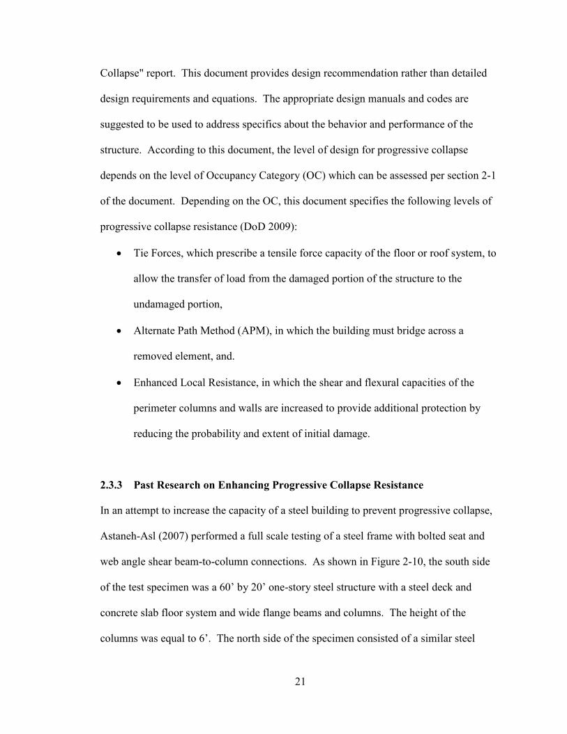
In an attempt to increase the capacity of a steel building to prevent progressive collapse,
Astaneh-Asl (2007) performed a full scale testing of a steel frame with bolted seat and
web angle shear beam-to-column connections. As shown in Figure 2-10, the south side
of the test specimen was a 60’ by 20’ one-story steel structure with a steel deck and
concrete slab floor system and wide flange beams and columns. The height of the
columns was equal to 6’. The north side of the specimen consisted of a similar steel
22
frame, but it contained catenary cables running longitudinal as seen in Figure 2-10.
These catenary cables were used to develop the catenary action under the vertical load
which would, ultimately, enhance the progressive collapse resistance of the frame. The
center columns on each longitudinal frames of the specimen were constructed 36 inches
above the laboratory floor. This action was taken to simulate the sudden lost of these
columns in the event of an explosion (columns C1 and C2 from Figure 2-10 were the two
columns removed). A hydraulic actuator pushing downward on the top of those two
columns was implemented to simulate the gravity loads on the column.
From the results shown in Figure 2-11 it is evident that the frame with the catenary cables
was able to resist higher load than the frame with no catenary cables. At the column
downward displacement of 27 inches; the catenary cables were supporting over half of
the column load. The investigator proposed to install the catenary cables as a method to
retrofit existing structures to enhance progressive collapse resistance.
Figure 2-10: Plan view of the tested specimen with catenary cables
(Astaneh-Asl 2007)

23
Figure 2-11: Test Results (Astaneh-Asl 2007)
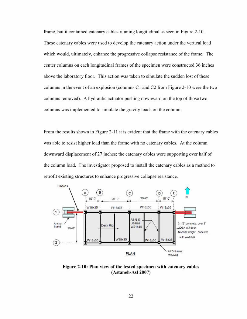
Although the catenary cable provides additional vertical load resistance after a sudden
column removal it would only work under specific circumstances. The catenary cables
would provide additional progressive collapse resistance only when an interior column is
removed due to an extreme event. In the case in which a corner column fails, the cables
may lose anchorage at the end and likely provide no additional catenary action. Note that
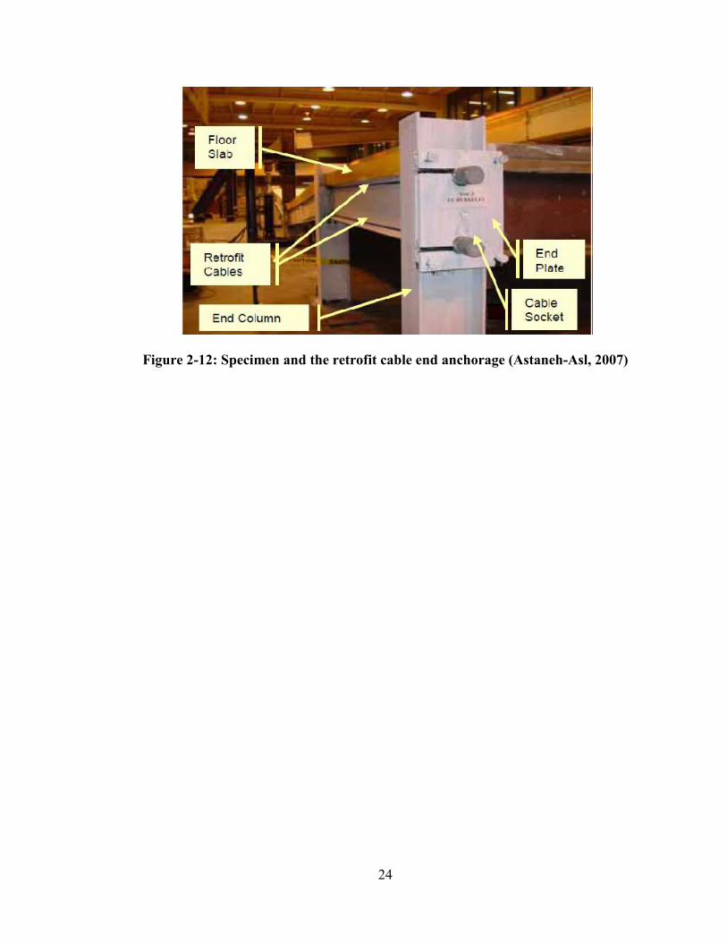
the exterior column corresponds to the end column shown in Figure 2-12. The DoD UFC
requires the removal of an exterior column as part of column removal strategy to evaluate
the building’s capacity to prevent progressive collapse. Figure 2-13 shows the diagram
outlining the column removal strategy by the DoD UFC. Therefore, the catenary cable
retrofitting technique does not meet the strategic column removal plan to evaluate the
systems progressive collapse resistance.
24
Figure 2-12: Specimen and the retrofit cable end anchorage (Astaneh-Asl, 2007)
25
Figure 2-13: Column removal strategy (DoD UFC 2009)
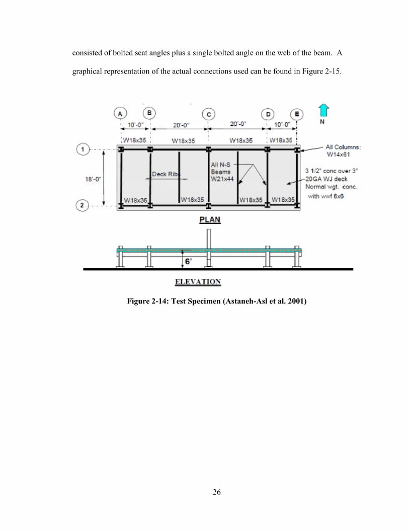
Astaneh-Asl et al. (2001) also investigated the contribution of simple beam-to-column
connections to the system progressive collapse resistance. The specimen consisted of a
60 foot by 20 foot one-story steel structure with a steel deck and concrete slab floor
system and wide flange beams and columns. Figure 2-14 shows schematics of the plan
and elevation views of the tested specimen. As seen on the elevation view the center
column corresponded to the removed column. The beam-to-column shear connections
26
consisted of bolted seat angles plus a single bolted angle on the web of the beam. A
graphical representation of the actual connections used can be found in Figure 2-15.
Figure 2-14: Test Specimen (Astaneh-Asl et al. 2001)

27
Figure 2-15: Beam-to-column connections (left) beam-to-girder connections (right)
(Astaneh-Asl et al. 2001)
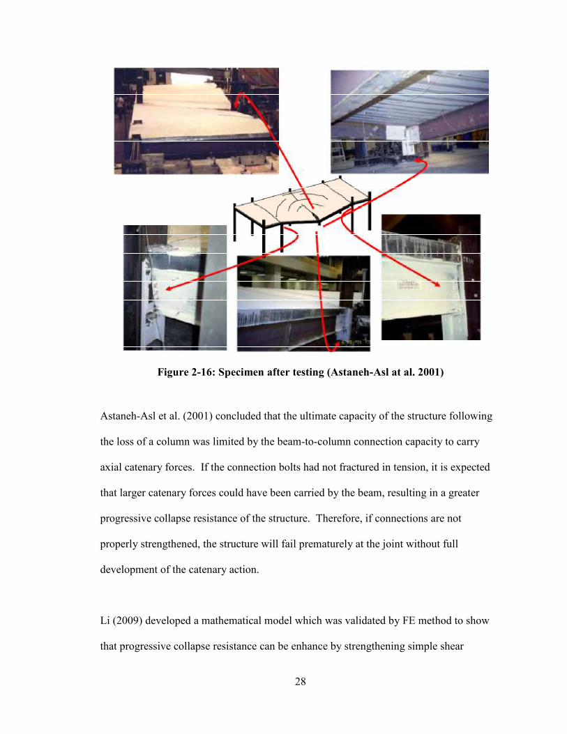
The specimen was loaded three times at the missing column by gradually increasing
vertical downward displacements to a maximum of 19, 24 and 35 inches respectively.
During the second loading it was observed that the bolts that held the longitudinal beam
east of the loaded column on the seated connection at column C2, failed. In addition, the
seated connection also yielded. Figure 2-16 shows the post-testing behavior of the
specimen. During the third loading and at approximately 26 inches of downward
displacement the connecting angles between the drop column C2 and the longitudinal
beam directly east completely failed. It was noted that after the connection failed the
concrete slab was transferring the applied force to the longitudinal beam east of the
displacing column.
28
Figure 2-16: Specimen after testing (Astaneh-Asl at al. 2001)
Astaneh-Asl et al. (2001) concluded that the ultimate capacity of the structure following
the loss of a column was limited by the beam-to-column connection capacity to carry
axial catenary forces. If the connection bolts had not fractured in tension, it is expected
that larger catenary forces could have been carried by the beam, resulting in a greater
progressive collapse resistance of the structure. Therefore, if connections are not
properly strengthened, the structure will fail prematurely at the joint without full
development of the catenary action.
Li (2009) developed a mathematical model which was validated by FE method to show
that progressive collapse resistance can be enhance by strengthening simple shear

29
connections. The researcher proposed two retrofitting techniques that would change the
partial-strength shear resisting joint to the full-strength moment resisting joints. Figure
2-17 shows the common design for fin plate shear joins of most steel structures.
Figure 2-17: Original design of fin plate joins (Li 2009)
Two retrofitting options were investigated. Retrofitting scheme 1 is similar to the flange
plate connection used in new structures (Li 2009). In addition to welding the beam flange
and the stiffener to the column as shown in Figure 2-18, the lapped flange plate was
connected to the flange of column and beam by butt welding and fillet welding,
respectively. The objective was to transfer the weakest cross-section away from the
beam-to-column joint and to improve the ductility, the continuity and the redundancy of
the structure (Li 2009).
30
Figure 2-18: Retrofitting scheme 1 (J.L. Li 2009)
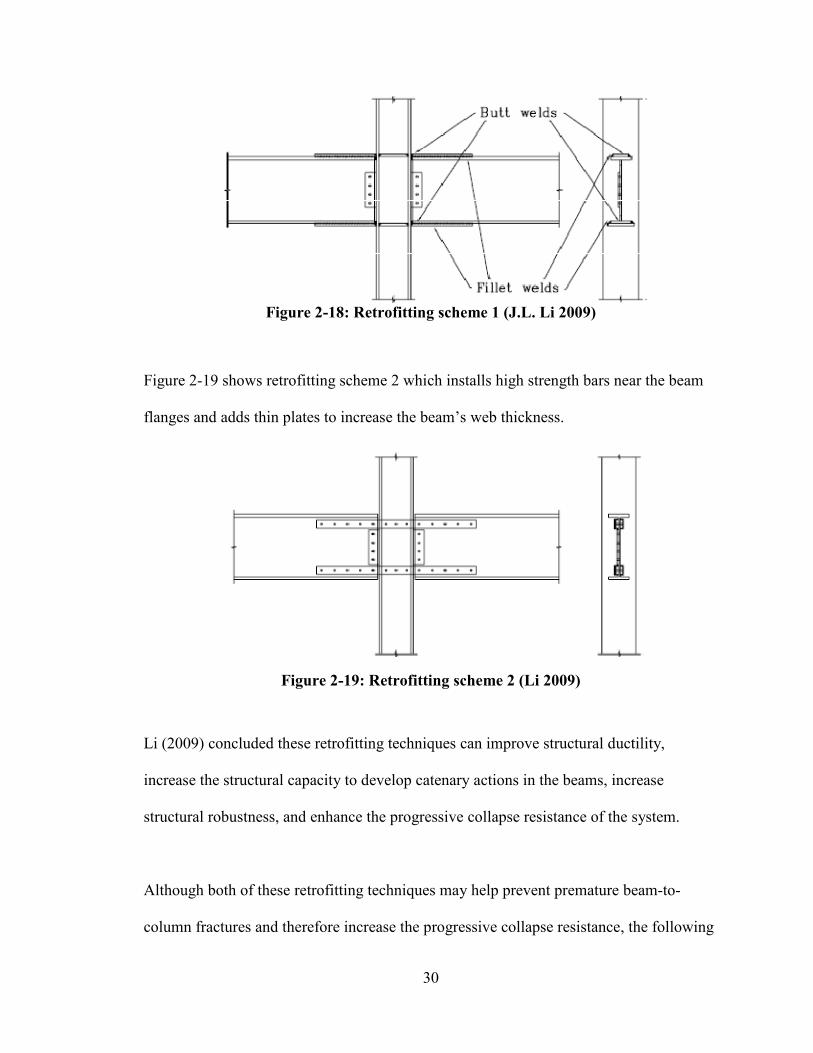
Figure 2-19 shows retrofitting scheme 2 which installs high strength bars near the beam
flanges and adds thin plates to increase the beam’s web thickness.
Figure 2-19: Retrofitting scheme 2 (Li 2009)
Li (2009) concluded these retrofitting techniques can improve structural ductility,
increase the structural capacity to develop catenary actions in the beams, increase
structural robustness, and enhance the progressive collapse resistance of the system.
Although both of these retrofitting techniques may help prevent premature beam-to-
column fractures and therefore increase the progressive collapse resistance, the following

31
disadvantages are identified. The first technique is labor intensive because it requires the
removal of the floor slab near the column in order to add the welds. In addition, the
quality of the weld can be compromised due to the inconvenient welding directions that
can be performed due to a space restriction of the already existing structure.
Furthermore, intensive welding can cause residual stress and can potentially cause non-
ductile damage of the columns and beams. The second retrofitting scheme requires many
holes to be drilled or punched on the existing columns and beams which can be labor
intensive and very difficult to accomplish on the site. In addition, these holes reduce the
net cross-section area of the beam decreasing its shear and tensile catenary capacities. By
implementing the connection retrofitting techniques suggested by Li or others, the
maximum progressive collapse resistance that can be obtained is equal to the tensile
strength of the beams. In the event in which the vertical load exceeds the tensile strength
of the beam, the beam can rupture triggering progressive collapse.
Other researchers have suggested the concept of structural compartmentalization and
isolation as a means to improve the system progressive collapse resistance. The idea is to
confine the structural damage to a small area. Based on this design philosophy, if
progressive collapse occurs only a small compartment of the entire structure will be
affected. Although this method can be feasible, compartmentalization requires small
spans and spaces with independent structural systems. In comparison with the common
continuity design, compartmentalization is significantly less efficient in terms of
constructability and space usage (Marchand & Alfawakhiri 2004). Furthermore,
32
compartmentalization does not prevent progressive collapse; instead it limits progressive
collapse damage to a small area of the entire structure.
2.4 Summary
An extensive literature review on analytical modeling of SPSWs and recent research
outcomes on progressive collapse is presented in this chapter. Emphasis was made on the
modeling of the infill panels. In addition, limitations of the current strategies for
progressive collapse retrofit of steel frames were identified.

33
3 PLASTIC ANALYSIS OF THE PROPOSED SYSTEM
3.1 Consideration of Initial Column Failure
Among the possible structural member damages in steel frame buildings, failures in
columns are more likely to initiate progress collapse since columns are the key members
to support and transfer the gravity loads acting on the frame to foundations. Past research
on structural progressive collapse caused by column failures can be divided into two
categories: the research focusing on the threat or loading mechanism causing the column
failure; and the investigations focusing on performance evaluation and retrofit of the
system vulnerable to collapse (Hoffman 2010). The second category is commonly
known as the threat independent approach in which the column that may be damaged is
removed from the system, i.e., assuming the damaged column surrenders all of its load-
carrying capacity. Although less accurate, this procedure is more versatile as the results
are valid for any abnormal loading (Hoffman 2010). In the case where the column’s
entire capacity is not lost, the threat-independent approach is more conservative because
it assumes that the column does not contribute any additional strength to the structure.
Figure 3-1 shows the collapse mechanism of a structure based on the threat independent
approach. Such an approach will be used in this thesis for assessing the performance of
the proposed system.
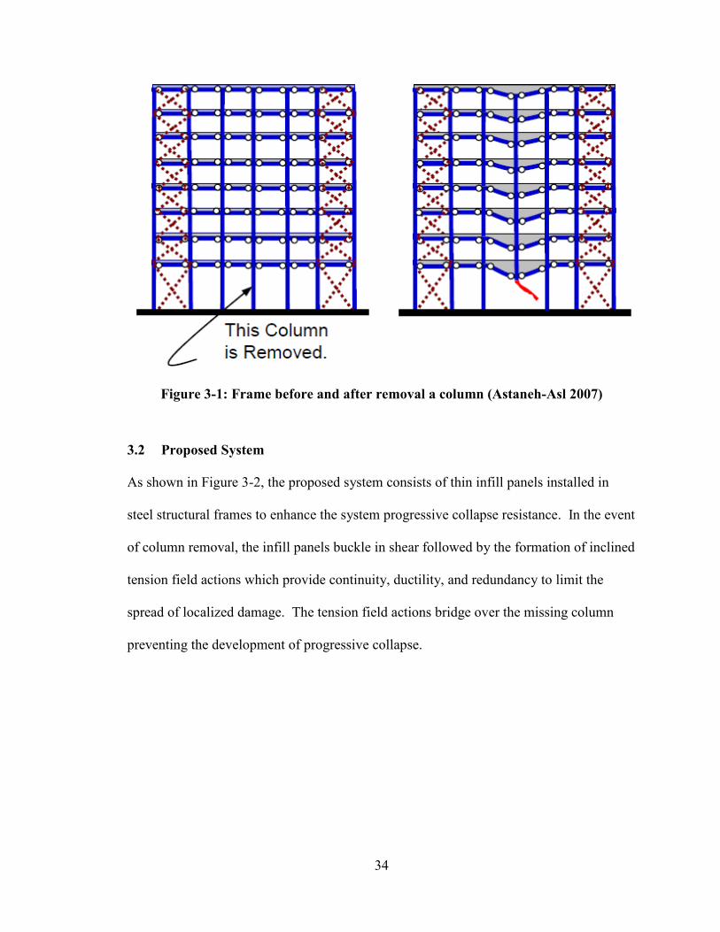
34
Figure 3-1: Frame before and after removal a column (Astaneh-Asl 2007)
3.2 Proposed System
As shown in Figure 3-2, the proposed system consists of thin infill panels installed in
steel structural frames to enhance the system progressive collapse resistance. In the event
of column removal, the infill panels buckle in shear followed by the formation of inclined
tension field actions which provide continuity, ductility, and redundancy to limit the
spread of localized damage. The tension field actions bridge over the missing column
preventing the development of progressive collapse.
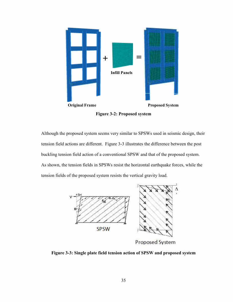
35
Figure 3-2: Proposed system
Although the proposed system seems very similar to SPSWs used in seismic design, their
tension field actions are different. Figure 3-3 illustrates the difference between the post
buckling tension field action of a conventional SPSW and that of the proposed system.
As shown, the tension fields in SPSWs resist the horizontal earthquake forces, while the
tension fields of the proposed system resists the vertical gravity load.
Figure 3-3: Single plate field tension action of SPSW and proposed system
Original Frame Proposed System
Infill Panels
+ =

36
The post buckling tension filed action on a multistory building for both, a SPSW and the
proposed system, can be found in Figure 3-4. The inclination of tension field action on
the multistory SPSWs helps resists the lateral loading. The inclination of the tension
field action of the proposed system in a multistory bridges the missing column and helps
arrest progressive collapse by transferring the load to the adjacent columns.
Figure 3-4: Tension field actions in multistory SPSWs and the proposed system
3.3 System Behavior
The behavior of the proposed system combines the infill panel tension field actions and
the boundary frame catenary actions if they are allowed to develop. This section
addresses the respective contributions of these two actions to the system progressive
collapse resistance based on the classic plastic analysis models developed by prior
researchers. The infill panels were analyzed using the strip model developed for
consideration of the tension field actions by Thorburn et al. (1983). Berman and Bruneau
(2003) confirmed the reliability of such a model for calculation of the SPSW plastic
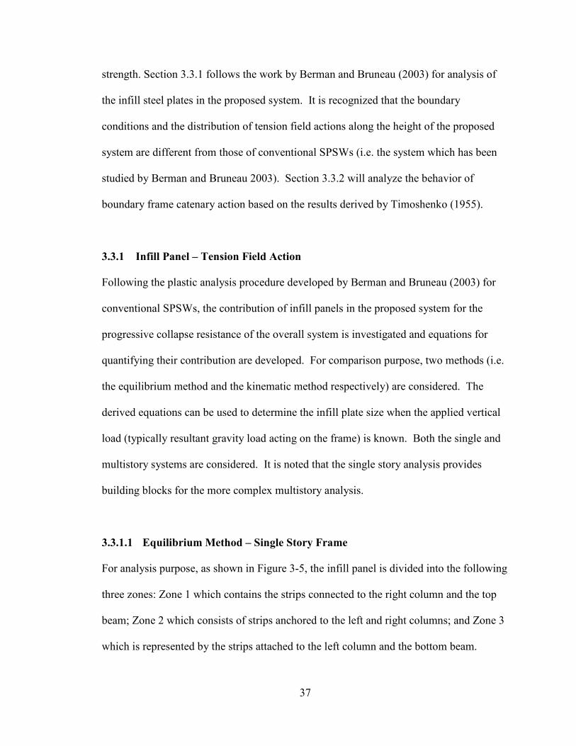
37
strength. Section 3.3.1 follows the work by Berman and Bruneau (2003) for analysis of
the infill steel plates in the proposed system. It is recognized that the boundary
conditions and the distribution of tension field actions along the height of the proposed
system are different from those of conventional SPSWs (i.e. the system which has been
studied by Berman and Bruneau 2003). Section 3.3.2 will analyze the behavior of
boundary frame catenary action based on the results derived by Timoshenko (1955).
3.3.1 Infill Panel – Tension Field Action
Following the plastic analysis procedure developed by Berman and Bruneau (2003) for
conventional SPSWs, the contribution of infill panels in the proposed system for the
progressive collapse resistance of the overall system is investigated and equations for
quantifying their contribution are developed. For comparison purpose, two methods (i.e.
the equilibrium method and the kinematic method respectively) are considered. The
derived equations can be used to determine the infill plate size when the applied vertical
load (typically resultant gravity load acting on the frame) is known. Both the single and
multistory systems are considered. It is noted that the single story analysis provides
building blocks for the more complex multistory analysis.
3.3.1.1 Equilibrium Method – Single Story Frame
For analysis purpose, as shown in Figure 3-5, the infill panel is divided into the following
three zones: Zone 1 which contains the strips connected to the right column and the top
beam; Zone 2 which consists of strips anchored to the left and right columns; and Zone 3
which is represented by the strips attached to the left column and the bottom beam.

38
Every zone is labeled and delineated by dash lines in Figure 3-5. The maximum
resistance of each zone (Pi) is found then added to determine the progressive collapse
resistance capacity of the entire infill panel.
Figure 3-5: Strip model of a single SPSW with simple beam-to-column connection
3.3.1.1.1 Zone 1:
The FBDs of Zone 1 are shown in Figure 3-6 and Figure 3-7.
Figure 3-6: Zone 1 FBD - Top beam and right column
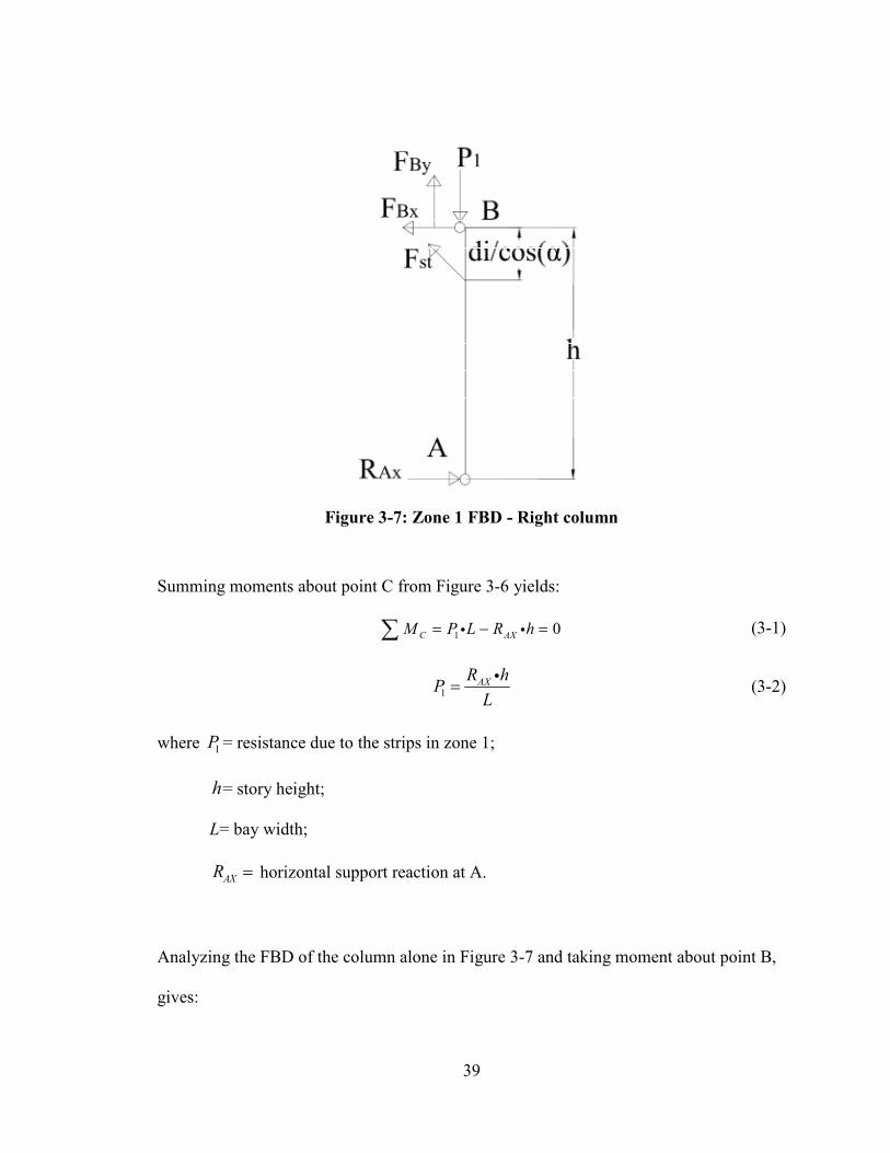
39
Figure 3-7: Zone 1 FBD - Right column
Summing moments about point C from Figure 3-6 yields:
1
0C AX
M P L R h= − =∑ i i (3-1)
1AX
R hP
L=
i
(3-2)
where 1P = resistance due to the strips in zone 1;
h= story height;
L= bay width;
AXR = horizontal support reaction at A.
Analyzing the FBD of the column alone in Figure 3-7 and taking moment about point B,
gives:
40
cos 0 cos
nB AX st
dM R h F α
α = − =
∑ i i i (3-3)
0nAX st
dR F
h
= = i (3-4)
where stF = force of one strip;
nd = perpendicular distance between the beam-column connection and the strip in
zone 1; and all the other parameters have been previously defined.
Substituting (3-4) into (3-2) results in:
1n st n std F h d F
PL h L
= =i i i
i
(3-5)
The resistance provided by one strip in zone one is:
1n std F
PL
=i
(3-6)
Therefore, the total resistance provided by all the strips in zone one can be represent by:
1
1
in st
n
d FP
L=
=∑i
(3-7)
where i = number of strips in zone 1; and all other parameters have been previously
defined.
3.3.1.1.2 Zone 2:
The FBDs of Zone 2 are shown in Figure 3-8 and Figure 3-9.

41
Figure 3-8: Zone 2 FBD - Top beam and right column
Figure 3-9: Zone 2 FBD - Right column
Summing the moments about point C and using the FBD in Figure 3-8 result in:
2 cos ( sin 0 cos
j
C AX st st
dM R h P L F h h F Lα α
α
= − − − − + =
∑ i i i i i i (3-8)
2 sinAX st j stP L R h F d F Lα= − +i i i i i (3-9)
Analyzing the FBD of the right column from Figure 3-9 yields:

42
0 B AX st j
M R h F d= − =∑ i i (3-10)
st j
AX
F dR
h=
i
(3-11)
where jd = perpendicular distance between the top right beam-column interface and the
distance to the strip in zone 2; and all the other variables have been previously defined
Substituting (3-11) into (3-9) gives:
2 sin
st j
st j st
F dP L h F d F L
hα= − +
i
i i i i i (3-12)
The resistance provided by one strip in zone 2 ( 2P ) is:
2 sinstP F α= i (3-13)
where α = the angle of inclination of the principal tensile stresses in the strips measured
from the horizontal.
The total resistance provided by the strips in Zone 2 becomes:
2
1
sinm
st
j
P F α=
=∑ i (3-14)
where m = number strips in zone two.
3.3.1.1.3 Zone 3
The FBDs of Zone 3 are shown in Figure 3-10.
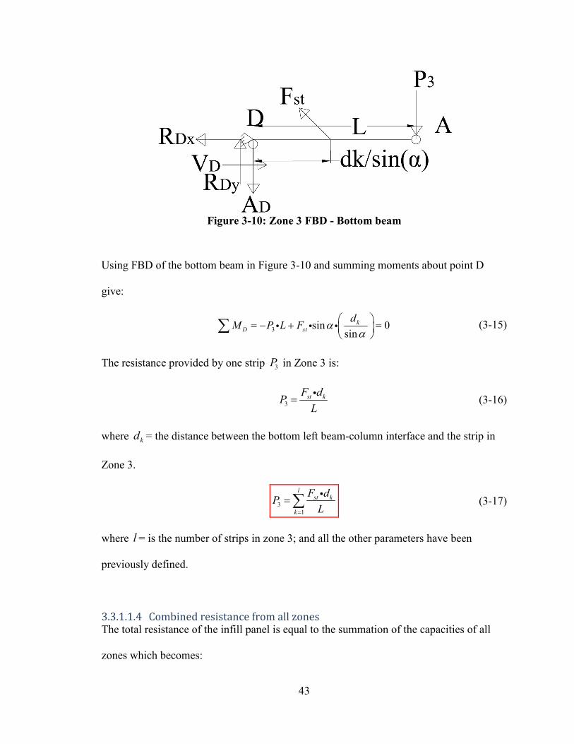
43
Figure 3-10: Zone 3 FBD - Bottom beam
Using FBD of the bottom beam in Figure 3-10 and summing moments about point D
give:
3 sin 0
sin
kD st
dM P L F α
α = − + =
∑ i i i (3-15)
The resistance provided by one strip 3P in Zone 3 is:
3 st kF dP
L=i
(3-16)
where kd = the distance between the bottom left beam-column interface and the strip in
Zone 3.
3
1
l
st k
k
F dP
L=
=∑i
(3-17)
where l = is the number of strips in zone 3; and all the other parameters have been
previously defined.
3.3.1.1.4 Combined resistance from all zones
The total resistance of the infill panel is equal to the summation of the capacities of all
zones which becomes:
44
1 2 3P P P P= + + (3-18)
Substituting the expression for the resistance of each zone gives:
1 1 1
sin i m l
n st st kst
n j k
d F F dP F
L Lα
= = =
= + +∑ ∑ ∑i i
i (3-19)
Knowing that Zones 1 and 3 have the same number of strips due to equal strip spacing
and from geometry of Figure 3-5 it is known that:
sinL
i ls
α= = (3-20)
cos sinh L
ms
α α−= (3-21)
From Figure 3-5 the distance from the upper right and the lower left strips are s/2 from
their respective beam-column interface, therefore the summation of dn and dk can be
express as follows:
2
1 1
2
i l
n k
n k
l sd d
= =
= =∑ ∑ (3-22)
Substituting equation (3-22) into(3-19), gives:
1 1 1
sin i m l
n kst
n j k
d dP F
L Lα
= = =
= + +
∑ ∑ ∑ (3-23)
2 2
1
sin2 2
m
st
j
l s l sP F
L Lα
=
= + +
∑
i i
(3-24)
Substituting equations(3-20), (3-21) into (3-24), gives:
2 2sin sin
cos sinsin
2 2st
L Ls s
h Ls sP F
L s L
α αα α
α
− = + +
i i
i (3-25)

45
2 2sin cos sin sinst
L h LP F
s s s
α α α α = + −
(3-26)
cos sin
st
hP F
s
α α =
(3-27)
Equation (3-28) represent the force in one strip:
platest y stripF f A= i (3-28)
where plateyf = plate tensile yield stress;
stripA = Area of one strip which is define by equation (3-29).
The area of a single strip is represented by (3-29).
strip plateA t s= i (3-29)
where platet = thickness of the plate;
s = spacing between strips
Equation (3-30) shows a trigonometric identity which will be used for simplification
purposes:
sin 2
sin cos2
αα α = (3-30)
Substituting equations(3-28),(3-29) and (3-30) into equation(3-27) yields:
1
sin 22
y plateP f t h α= i i i (3-31)
It is noted that the total capacity provided by the infill panel is directly proportional to the
height of the infill panel.

46
3.3.1.2 Kinematic Method – Single Story Frame
The strength of a sing-story frame with infill steel panels derived in Section 3.3.1.1 can
be equivalently obtained using another approach, i.e., kinematic method. Such a
derivation is presented in this section to confirm the adequacy of equation (3-31).
Figure 3-11 : Kinematic collapse mechanism single story tension field action
Assuming downward direction to be positive, from Figure 3-11 the external work done is
equal to:
externalW P= ∆i (3-32)
where ∆ = vertical displacement of the right column which excites the tension field
action
P = plastic strength of the single story frame with infill plates.
The beams and columns are assumed to remain elastic in the proposed system. As a
result, their contribution to the internal work is negligible compared with the internal
work done by the yielded strips. The internal energy in each strip is equal to the yielding
47
force multiplied by the corresponding displacement which can be decomposed into
horizontal and vertical components. Note that in the vertical direction the internal work
done by the strips attached to the top beams is positive while the internal work done by
the strips anchored to the bottom beam is negative due to the direction of the force in the
strips; therefore their net internal work is zero. In addition, along the horizontal
direction, the work done by any yielding force is zero because there is no displacement in
that direction under the small deformation assumption. Consequently, the vertical
component of the tension fields anchored to the right column has the only contribution to
the internal work of the system. Therefore, the internal work of the system becomes:
( )int sinplateernal c strip yW n A f α= ∆ (3-33)
where cn = number of strips anchored to the right column; and all the other parameters
have been previously defined.
From Figure 3-5:
cos
c
hn
s
α= (3-34)
Equating the external work to the internal work gives:
( )sinplatec strip yn A f Pα ∆ = ∆i (3-35)
Substituting equations(3-28),(3-29), (3-30) and (3-34) into equation(3-35) yields:
1
sin 22
y plateP f t h α= i i i (3-36)

48
Comparing equations (3-31) and (3-36), it is evident that the two methods considered
here (i.e. the equilibrium method and the kinematic method) provide the same prediction
of the progressive collapse resistance of infill plate in a single story frame.
3.3.1.3 Kinematic Method – Multistory Frame
Figure 3-12: Tension field distributions in a multistory frame subjected to sudden
column loss
On the basis of the results of infill plates in a single story frame presented in Section
3.3.1.2, the strength of infill plates in a multistory frame is investigated in this section.
The tension field distribution as represented by the diagonal strips in a multistory frame is
illustrated in Figure 3-12. Accordingly, the external work is:
externalW P= ∆i (3-37)
All the infill panels in the multistory frame are subjected to the same vertical
displacement, therefore the internal work is:
( ) ( )1 6int sin ... sinernal c st c stW n F n Fα α= ∆ + + ∆ (3-38)

49
( )1 2 3 4 5 6int sinernal c st st st st st stW n F F F F F Fα= ∆ + + + + +i i (3-39)
Substituting equations(3-28),(3-29), (3-30) and (3-34) into equation(3-39) yields:
( )1 2 3 4 5 6int
1sin 2
2ernal y pt pt pt pt pt ptW f h t t t t t tα= ∆ + + + + +i i i i (3-40)
int
1
1sin 2
2 i
n
ernal y pt
i
W f h tα=
= ∆
∑i i i i (3-41)
Equating the external work calculated by equations (3-37) to the internal work by
equation (3-41) gives:
1
1sin 2
2 i
n
y pt
i
P f h tα=
=
∑i i i (3-42)
where, n = number of plates contributing to the internal work of the multistory structure
iptt = the thickness of the ith
plate.
3.3.2 Boundary Frame Members - Catenary Actions
The catenary action in boundary frame members has been investigated by Timoshenko
(1955) and Astaneh-Asl (2007). Their analysis assumes that a multi-span frame
subjected to sudden removal of an interior column is equipped with a sufficient lateral
load resisting system which would prevent frame sway in the horizontal direction. Such
assumption allows the catenary force T to develop in the beam segments which would
provide the vertical resistance of the system against collapse. The analysis presented here
was originally derived by Timoshenko (1955) to develop the load-displacement
relationship for elastic beam members.
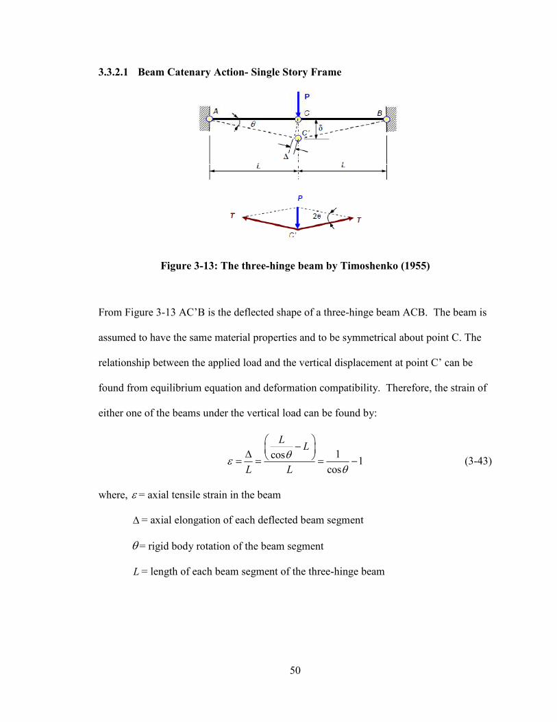
50
3.3.2.1 Beam Catenary Action- Single Story Frame
Figure 3-13: The three-hinge beam by Timoshenko (1955)
From Figure 3-13 AC’B is the deflected shape of a three-hinge beam ACB. The beam is
assumed to have the same material properties and to be symmetrical about point C. The
relationship between the applied load and the vertical displacement at point C’ can be
found from equilibrium equation and deformation compatibility. Therefore, the strain of
either one of the beams under the vertical load can be found by:
1cos
1cos
LL
L L
θεθ
− ∆ = = = − (3-43)
where, ε = axial tensile strain in the beam
∆ = axial elongation of each deflected beam segment
θ= rigid body rotation of the beam segment
L = length of each beam segment of the three-hinge beam
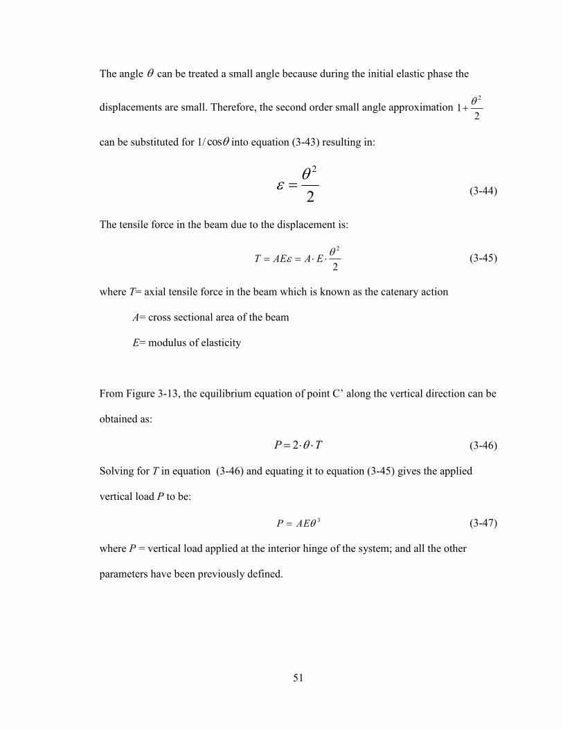
51
The angle θ can be treated a small angle because during the initial elastic phase the
displacements are small. Therefore, the second order small angle approximation 2
12
θ+
can be substituted for 1/ cosθ into equation (3-43) resulting in:
2
2
θε = (3-44)
The tensile force in the beam due to the displacement is:
2
2T AE A E
θε= = ⋅ ⋅ (3-45)
where T= axial tensile force in the beam which is known as the catenary action
A= cross sectional area of the beam
E= modulus of elasticity
From Figure 3-13, the equilibrium equation of point C’ along the vertical direction can be
obtained as:
2P Tθ= ⋅ ⋅ (3-46)
Solving for T in equation (3-46) and equating it to equation (3-45) gives the applied
vertical load P to be:
3P AEθ= (3-47)
where P = vertical load applied at the interior hinge of the system; and all the other
parameters have been previously defined.

52
Substituting L
δfor θ in equation (3-47) yields the vertical displacement δ as a function
of the vertical applied load P to be:
3P
LA E
δ = ⋅⋅
(3-48)
This equation suggests that the relationship between the vertical load and the vertical
displacement is nonlinear. Solving for θ in equation (3-46) gives:
2
P
Tθ =
⋅ (3-49)
Substituting equation (3-49) into equation (3-47) and solving for the catenary force T
gives the following:
2
3
8
P A ET
⋅ ⋅= (3-50)
Figure 3-14: Force-displacement relationship for a three-hinge beam Astaneh-Asl
(2007)

53
A graphical representation of Timoshenko's force-displacement relationship for a three
hinge beam is shown in Figure 3-14. Astaneh-Asl (2007) used those results to find the
beams elastic strain energy eU :
0
eU P d
δ
δ= ⋅∫ (3-51)
Solving for P in terms of δ in equation (3-48) and substituting those results into equation
(3-51) yields:
43 3
3 3
04 4 4
e
A E A E P P L PU d
L L AE
δ δ δδ δ
⋅ ⋅ ⋅ ⋅ ⋅= ⋅ = = = ⋅∫ (3-52)
where, eU = the elastic strain energy of the three-hinge beam;
dδ = incremental vertical displacement under the applied load P.
The above derived equation is valid when the system remains elastic. The following
equations should be considered for the cross-section when the first yielding occurs in the
system:
y
y
F
Eε = (3-53)
2
2y
y y
F
Eθ ε
⋅= ⋅ = (3-54)
y y yT AE AFε= = (3-55)
8
2y
y y y y
FP T A F
Eθ
⋅= ⋅ ⋅ = ⋅ ⋅ (3-56)
32
y y
y
P FL L
A E Eδ
⋅= ⋅ = ⋅
⋅ (3-57)

54
where, yε = yield strain;
yF = yield stress;
yT = axial tensile yield capacity;
yP = applied vertical load at time of yielding;
yθ = rigid body rotation of the beam at yielding;
yδ = vertical displacement under applied load at the time of yielding of the beam.
Assuming no strain hardening, the axial force in the beam remains constant at Ty while
the applied load P continue to increase due to an increase in the vertical deflection
(Astaneh-Asl 2007). Figure 3-15 presents the force-displacement relationship beyond the
beam’s yielding point. Note that the horizontal axis shows the vertical displacement
normalized by the beam length. The post yield region becomes linear due to no
additional resistance contribution due to the beam’s catenary forces.
Figure 3-15: Force-displacement relationship for a three hinge beam beyond its
yield point (Astaneh-Asl 2007)
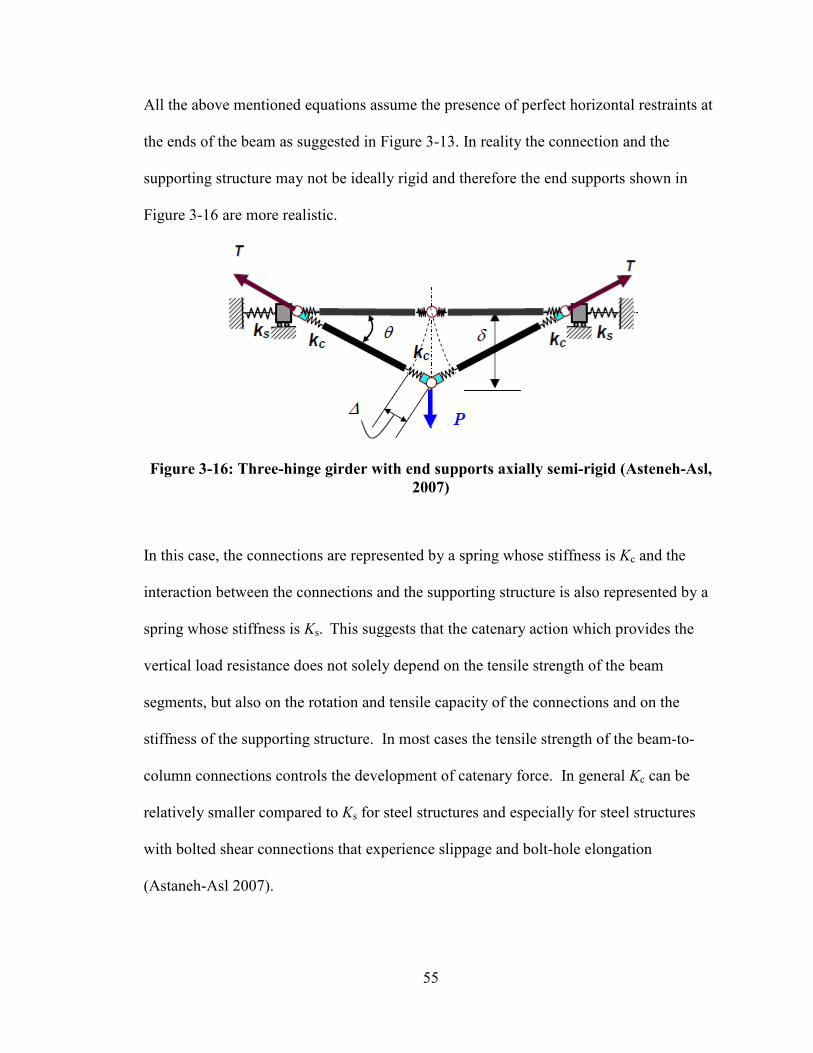
55
All the above mentioned equations assume the presence of perfect horizontal restraints at
the ends of the beam as suggested in Figure 3-13. In reality the connection and the
supporting structure may not be ideally rigid and therefore the end supports shown in
Figure 3-16 are more realistic.
Figure 3-16: Three-hinge girder with end supports axially semi-rigid (Asteneh-Asl,
2007)
In this case, the connections are represented by a spring whose stiffness is Kc and the
interaction between the connections and the supporting structure is also represented by a
spring whose stiffness is Ks. This suggests that the catenary action which provides the
vertical load resistance does not solely depend on the tensile strength of the beam
segments, but also on the rotation and tensile capacity of the connections and on the
stiffness of the supporting structure. In most cases the tensile strength of the beam-to-
column connections controls the development of catenary force. In general Kc can be
relatively smaller compared to Ks for steel structures and especially for steel structures
with bolted shear connections that experience slippage and bolt-hole elongation
(Astaneh-Asl 2007).

56
Figure 3-17: Vertical load resistance vs. beam cross-sectional area
Figure 3-17 is a graphical representation of the vertical load resistance at the time of the
first yield of the two beams adjacent to the missing column with respect to their cross-
sectional areas. A linear relationship was observed. It is noted that this graph assumes
constant vertical displacement normalized by the beam's length to be .05 and constant
elastic modulus of 29000 (ksi). In addition, the catenary action in the beams was fully
developed due to the ideally rigid connection and supporting structure.
3.3.2.2 Beam Catenary Action-Multistory Frame
The same assumption used to derive the catenary action of the three hinge beam can
apply to the multistory frame case. Similar to the single story frame, the following
assumptions were made for multistory frames: 1) the frame is subjected to a sudden
column removal; 2) the connections allow catenary action to develop in the beams; 3) the
frame is equipped with a sufficiently rigid lateral load resistance system which would
0
100
200
300
400
500
600
700
800
900
1000
0 50 100 150 200 250 300
Ve
rtic
al
loa
d r
esi
sta
nce
(k
ips)
Cross-sectional area (in2)
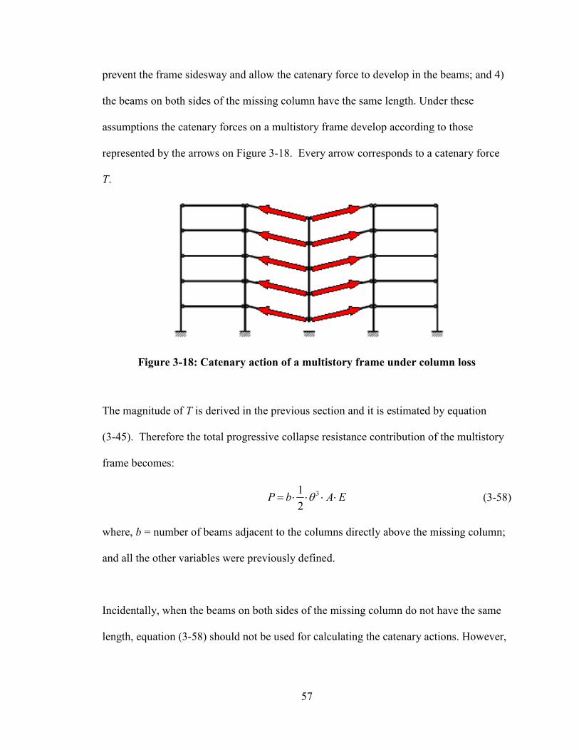
57
prevent the frame sidesway and allow the catenary force to develop in the beams; and 4)
the beams on both sides of the missing column have the same length. Under these
assumptions the catenary forces on a multistory frame develop according to those
represented by the arrows on Figure 3-18. Every arrow corresponds to a catenary force
T.
Figure 3-18: Catenary action of a multistory frame under column loss
The magnitude of T is derived in the previous section and it is estimated by equation
(3-45). Therefore the total progressive collapse resistance contribution of the multistory
frame becomes:
31
2P b A Eθ= ⋅ ⋅ ⋅ ⋅ (3-58)
where, b = number of beams adjacent to the columns directly above the missing column;
and all the other variables were previously defined.
Incidentally, when the beams on both sides of the missing column do not have the same
length, equation (3-58) should not be used for calculating the catenary actions. However,

58
if needed, the equations corresponding to such cases can be similarly derived using the
presented FBDs and procedures.
3.3.3 Combination of Tension Fields and Catenary Actions
The system progressive collapse resistance respectively provided by the infill panel
tension field actions and the boundary frame catenary actions can be found by adding
equations (3-41) and (3-58) to get:
3
1
1 1sin 2
2 2i
n
y pt
i
P f h t b A Eα θ=
= + ⋅ ⋅ ⋅ ⋅
∑i i i (3-59)
3.4 Summary
This chapter describes the proposed system and its plastic behavior under sudden column
removal. The progressive collapse resistance of this system was quantified by equation
(3-59) which combines the contributions of the infill plate tension field actions and the
boundary frame catenary actions. Results from this chapter will be verified by FE results
presented in the subsequent chapters.

59
4 DEVELOPMENT OF HIGH-FIDELITY ANALYTICAL MODELS
4.1 Introduction
In order to validate the analytical models derived in Chapter 3 for calculation of the
progressive collapse resistance of the proposed system, high-fidelity FE models were
developed and analyzed. Two FE models were considered and these two models require
different modeling efforts and have different levels of accuracy. The first model is a 3D
FE model developed using the commercially available simulation software package,
ABAQUS 6.10 (Simulia 2008). This model explicitly models the infill plates and is able
to capture the plate buckling behavior . The second model is a simplified 2D FE model
developed using another commercially available simulation software package, SAP2000,
which represents the infill panels with diagonal strips based on the concept of strip model
proposed by Thorburn et al. (1983). This chapter presents in detail the procedure and
modeling techniques used to develop both models.
4.2 Demonstration Structure
The FE models described in this chapter were developed according to a demonstration
steel frame structure which consists of a four-story two-span frame retrofitted with the
infill panels. As shown in Figure 4-1, the damaged column at the bottom story which
may trigger progressive collapse of the system was omitted to provide an initial condition
for the analysis. Incidentally, both the damages in interior and exterior columns are
considered in this thesis although Figure 4-1 only shows the interior column removal.
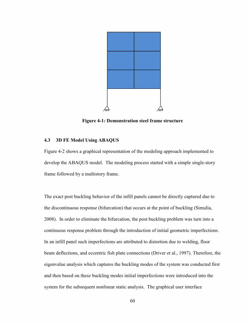
60
Figure 4-1: Demonstration steel frame structure
4.3 3D FE Model Using ABAQUS
Figure 4-2 shows a graphical representation of the modeling approach implemented to
develop the ABAQUS model. The modeling process started with a simple single-story
frame followed by a multistory frame.
The exact post buckling behavior of the infill panels cannot be directly captured due to
the discontinuous response (bifurcation) that occurs at the point of buckling (Simulia,
2008). In order to eliminate the bifurcation, the post buckling problem was turn into a
continuous response problem through the introduction of initial geometric imperfections.
In an infill panel such imperfections are attributed to distortion due to welding, floor
beam deflections, and eccentric fish plate connections (Driver et al., 1997). Therefore, the
eigenvalue analysis which captures the buckling modes of the system was conducted first
and then based on these buckling modes initial imperfections were introduced into the
system for the subsequent nonlinear static analysis. The graphical user interface
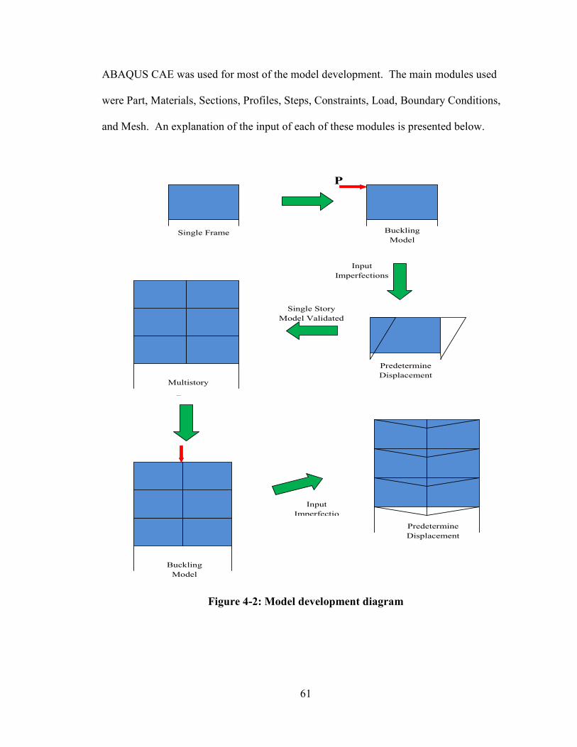
61
ABAQUS CAE was used for most of the model development. The main modules used
were Part, Materials, Sections, Profiles, Steps, Constraints, Load, Boundary Conditions,
and Mesh. An explanation of the input of each of these modules is presented below.
Figure 4-2: Model development diagram
Predetermine
Displacement
Input
Imperfections
Multistory
Frame
Buckling
Model
P
Buckling
Model
Single Frame
Predetermine
Displacement
Single Story
Model Validated
Input
Imperfectio

62
4.3.1.1 Parts
Three different parts were created for the development of the single story simulation,
namely beam, column and infill panel. The beam and column consisted of a 3D
deformable type with basic features, shape, and type consisting of wire and planar,
respectively. The infill panel part was created using a 3D deformable type with basic
features, shape and type consisting of shell and planar, respectively. Using the assembly
module these three parts was included multiple times to generate the necessary number of
beams, columns and infill panels. Defining the material's properties was the subsequent
step in developing the FE model.
4.3.1.2 Materials
In this analysis, the steels used in boundary frame and infill panels are assumed to be
both elastic-perfectly plastic but with different yield stresses. As such, two materials
were defined in the materials module. The first material with higher yield strength (50
ksi) was created for the boundary frame elements (BFEs) (e.g. beams and columns) and
the second with lower yield strength (36 ksi) was defined for the infill panel. The elastic
properties assigned to both materials consisted of Young's Modulus of 29000000 psi and
Poisson's ratio of 0.3. For the plastic material properties, the plastic strain with the
magnitude of zero was assigned to both material models to ensure the elastic-perfectly
plastic property. Both materials were modeled to be isotropic together with a simple rate
independent constitutive behavior. In addition, the von mises yield surface was used as
the yield criterion. These material properties were assigned to the sections describe in
Section 4.3.1.3.
63
4.3.1.3 Section
Beam and shell sections were created for the BFEs and the infill panels, respectively.
The infill plate thickness was assumed to be .118 in (i.e., 3mm). It is noted that such
plates may not be available in the AISC section database; however, the results obtained
from this analysis can be used to validate the equations derived in the Chapter 3. The
beam sections were defined similarly using the section profiles described in Section
4.3.1.3.
4.3.1.4 Profile
The profile consisted of the cross section corresponding to a W36-256 provided by the
AISC Steel Construction Manual (AISC 2005). The focus of the model was on the
inelastic behavior of the infill panels; therefore an elastic boundary element which is
ensured by the large cross-sections was selected. A ratio of the cross-sectional areas of
the boundary frames to the infill panel was approximately 3.55. Such a big ratio allowed
for stiff boundary and facilitated the appreciation of the post buckling behavior of the
infill panel.
4.3.1.5 Step
Abaqus/Standard uses the Riks method to solve the buckling problems. In order to
accurately capture the post buckling behavior of the infill panels, the model was
subjected to two different step procedures. The buckling modes were determined through
a linear perturbation analysis. The buckling modes acquired were then used to introduce

64
the infill plate imperfections into the post buckling analysis model which was modeled
using a static, general step corresponding to a general procedure type. For this step the
nonlinear geometry was turn on and the automatic stabilization consisted of an energy
fraction of 0.0002 for convergence purpose.
4.3.1.6 Constraints
The ABAQUS/CAE interface provides a wide variety of constraints, but all of the
member to member interactions for this model were defined through the Tie displacement
constraint. ABAQUS allows for two Tie formulations, namely, surface-to-surface
formulation, and a node-to-surface formulation. Surface-to-surface formulation was
implemented to define all the interactions between all parts of the model. This
formulation requires no common joints between the two constrained parts. This
constraint requires one surface to be defined as master surface and the other as the slave
surface. The boundary displacement of the part containing the surface defined as master
is imposed to the part containing the surface defined as slave to ensure the deformation
compatibility between the two parts.
The columns were defined as master when connected to the beams. For the interaction
between the BFEs the tie rotational degree of freedoms was turn off to allow for free
rotation in beam-to-column connections (i.e., simple shear connections were considered
here). For the interaction between the BFEs and the infill panel, the BFEs were selected
as master surface and the infill panel as the slave surface. In this case the tie rotational
degree of freedom was turn on to simulate the welded connections between the infill
65
panel and the BFEs. It is noted that if the rotational degree of freedom is turn off the
buckling analysis of the infill panel would yield inaccurate results or plate buckling
would not occur.
4.3.1.7 Load
For the buckling mode analysis, a load of 1 kip was applied vertically downward on
every beam-column connection above the removed column. This loading direction
yielded the buckling shape of the infill panels under sudden column removal.
For the subsequent nonlinear static analysis (i.e. push-down analysis), a predetermined
displacement was assigned to all the columns above the missing column. A ratio of the
downward vertical displacement (∆) to the bay width (L) of 5% was used as the target
downward displacement. As such, the bay width of 180 in the example model yielded a
displacement of 9 in.
4.3.1.8 Boundary Conditions
Pin boundary conditions were applied to the nodes at the base of the columns. In
addition, the out-of-plane displacement of the floor levels was restricted. This was model
by setting the displacement in the out-of-plane direction equal to 0 for all the nodes of
beams. The horizontal motion restriction if necessary was modeled by restricting the
horizontal motion at the end of the short beam outriggers assigned at every exterior
beam-to-column connections. It is noted that both the sidesway inhibited and sideway
66
uninhibited boundary conditions were considered in this thesis and more detailed
descriptions about these boundary conditions are presented in Chapter 5.
4.3.1.9 Mesh
Each of the parts developed in section 4.3.1.1 were meshed individually. For the
boundary frame members a 2-node linear beam element (B31) was assigned. This
element type allows for transverse shear deformation, three translational degrees of
freedom ux, uy, and uz and three rotational degrees of freedom θx, θy, and θz at each end
of the element. Furthermore, B31 elements can be subjected to large axial strains which
allows for the accurately modeling of the development of catenary action of the beam.
The infill panels were modeled using the S4R element which consists of 4-node doubly
curved thin or thick shell, reduced integration, hourglass control, and finite membrane
strains. The S4R element formulation allows for thickness changes as a function of in-
plate deformation. Also, they do not have any unconstrained hourglass modes and do not
experience transverse shear locking. The S4R strain formulation provides accurate
solutions for in-plane bending behavior (Simulia, 2008). In addition, this element yields
accurate response when undergoing large-scale buckling behavior, which involves small-
strains but large rotations and severe bending.
The seeding was assigned to the boundary elements and infill panels using the built-in
function-global seeding in the ABUQUS/CAE interface. An approximate global seeding
size of 5 was selected for both, the boundary frame elements and the infill panels. The
67
edge length of any of the parts divided by the global seeding number would yield the
number of elements along that edge. A total of 36 elements were assigned to each
boundary frame member whereas each infill panel was modeled using 1296 elements.
4.4 Strip Model using SAP2000
The actual behavior of the system can be appreciated using the 3D FE model in
ABAQUS, but such a modeling procedure is too onerous and can be computationally
expensive for multi-story frames. In addition, the preprocessor and postprocessor of
ABAQUS are not as friendly as those used by conventional practicing engineers.
Therefore, a need exists to develop a more practical and simple model to simulate the
behavior of the proposed system.
Based on the strip model developed by Thorburn et al. (1983), a simplified 2D FE model
was developed in the commercially available software package SAP2000 for the
proposed system. In the strip model, the boundary frames were considered by beam-
column elements and the diagonal strips were considered by truss elements.
This section provides a detail explanation of the model development.
The angle of inclination of each strip was found using equation(4-1) per the NEHRP
Recommended Provisions and Commentary for Seismic Regulations for New Buildings
and Other Structures (Federal Emergency Management Agency, 2004). Note that for
multistory structures Ab, Ac and Ic were taken as the average of the two adjacent floors.
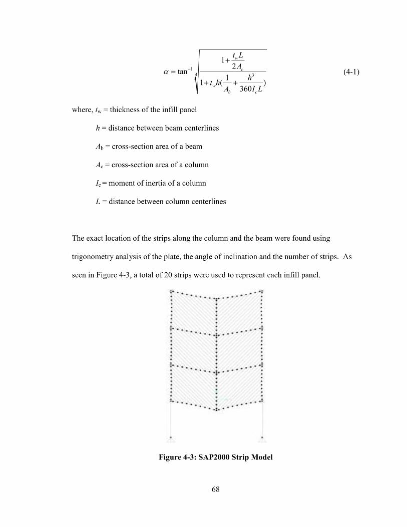
68
1
4 3
12
tan1
1 ( )360
w
c
w
b c
t L
A
ht h
A I L
α −
+=
+ + (4-1)
where, tw = thickness of the infill panel
h = distance between beam centerlines
Ab = cross-section area of a beam
Ac = cross-section area of a column
Ic = moment of inertia of a column
L = distance between column centerlines
The exact location of the strips along the column and the beam were found using
trigonometry analysis of the plate, the angle of inclination and the number of strips. As
seen in Figure 4-3, a total of 20 strips were used to represent each infill panel.
Figure 4-3: SAP2000 Strip Model
69
4.4.1 Parts
All the parts that constitute the formation of the entire frame were developed using the
node and line icons on the SAP2000 user interface. First, the nodes for the boundary
elements were drew and placed on their corresponding coordinates. Then the lines
connecting all the boundary nodes, which represent the boundary elements, were added.
Nodes along the columns and beams were added to serve as the connections between the
strips and the boundary frame. Finally, the strips were added by connecting the node on
the beams to its corresponding node on the columns.
4.4.2 Restrains
Consistent with the 3D FE model in ABAQUS, the translational deformations in the x, y,
and z directions was restrained at the two column base nodes to simulate pin connections
at the foundation. Additional restrains were added on the column nodes at each floor
level, depending on the case being investigated. All investigated cases will be explained
in the subsequent chapter. The strip-to-boundary-frame and beam-to-column connections
were modeled as hinges (i.e. setting the frame member partial fixity spring equal to zero
for major and minor moments, and torsions).
4.4.3 Materials
Two material properties were created. The material assigned to the boundary frames was
the A992Fy50 which is defined by default in the materials module of SAP 2000. This
material has minimum yield strength of 50 ksi and the effective yield strength was also
set to 50 ksi because the program uses the effective yield stress to compute the member
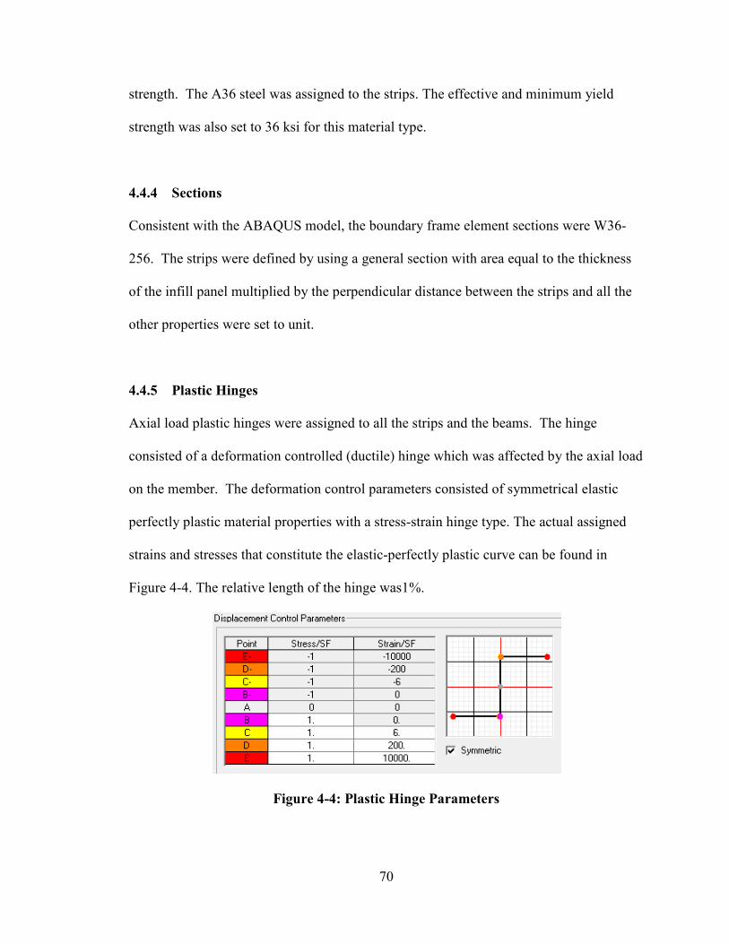
70
strength. The A36 steel was assigned to the strips. The effective and minimum yield
strength was also set to 36 ksi for this material type.
4.4.4 Sections
Consistent with the ABAQUS model, the boundary frame element sections were W36-
256. The strips were defined by using a general section with area equal to the thickness
of the infill panel multiplied by the perpendicular distance between the strips and all the
other properties were set to unit.
4.4.5 Plastic Hinges
Axial load plastic hinges were assigned to all the strips and the beams. The hinge
consisted of a deformation controlled (ductile) hinge which was affected by the axial load
on the member. The deformation control parameters consisted of symmetrical elastic
perfectly plastic material properties with a stress-strain hinge type. The actual assigned
strains and stresses that constitute the elastic-perfectly plastic curve can be found in
Figure 4-4. The relative length of the hinge was1%.
Figure 4-4: Plastic Hinge Parameters
71
Note that the plastic hinge was assigned on the center of every strip and at 10% of the
length of the beam from each end.
4.4.6 Load
One load pattern was created with a dead load type and a self weight multiplier of one.
Also, a linear static load case was used to assign a concentrated downward force of two
kips on each floor level node above the missing column. A nonlinear static load was
created to model the drop of the structure due to the removal of the column. Geometry
nonlinearly parameters were assigned to consider p-delta and large deformation effects.
The target downward displacement was selected to be 9 inches and it was assigned to the
node connecting the removed column.
4.5 Summary
The modeling procedures and details of two FE models are presented in this chapter. The
main objective of modeling the system using ABUQUS was to observe the actual
behavior of the system with consideration of plate buckling. Modeling of the system
using SAP2000 was more practical and such a model is able to provide results similar to
the ABAQUS model as will be discussed in Chapter 5. The strip model in SAP2000
which is more convenient will be used for most of the parametric investigations. Results
from the SAP2000, ABAQUS and plastic analysis models will be compared in Chapter 5.

72
5 DISCUSSION AND COMPARISON OF RESULTS FROM DEVELOPED
ANALYTICAL MODELS
5.1 Introduction
This chapter compares the system progressive collapse resistance using the models
developed in Chapters 3 and 4. Results for the original frame are also presented to
confirm the effectiveness of the proposed system. Note that the original frame refers to
the frame without any infill panels, while the retrofitted system refers to the proposed
system (i.e. the frame with infill panels).
5.2 Considered Boundary Conditions
Figure 5-1 presents the different boundary conditions for which the global behavior was
quantified for both the original frame and the retrofitted system. A total of five Boundary
Conditions (i.e. Boundary Conditions #1 through 5) were considered. Boundary
Conditions #1 through 3 corresponded to the scenarios of losing the interior column of
the frame while Boundary Conditions #4 and 5 took into account the loss of an exterior
column. For Boundary Condition #1 sidesway was uninhibited on both sides of the
frame. Boundary condition #2 inhibits sidesway deflection on one side of the frame,
assuming the presence of an infinitely rigid lateral load resisting system, while the other
side of the frame allows sidesway deflection. Boundary condition #3 inhibits sidesway
on both sides of the frame imitating infinitely rigid lateral load resisting systems on both
sides of the frame. Condition #4 allows sidesway while condition #5 inhibits sidesway
deflection. For quantification of the system vertical load resistance, all the five boundary
conditions were investigated in the nonlinear push down analysis in which a downward
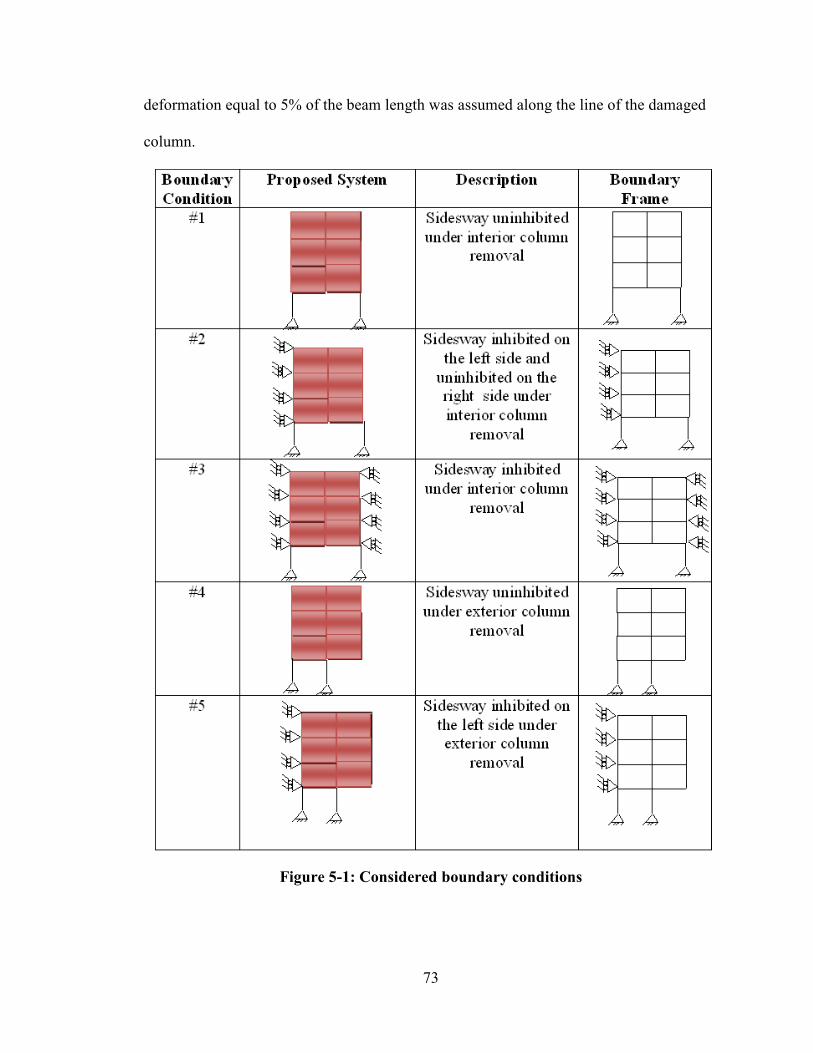
73
deformation equal to 5% of the beam length was assumed along the line of the damaged
column.
Figure 5-1: Considered boundary conditions

74
5.3 Discussion and Comparison of Results
5.3.1 Boundary Condition #1
Boundary Condition #1 corresponds to the system under interior column removal and
sidesway uninhibited on both sides of the frame. As discussed in Section 4.3, the FE
modeling of the system using ABAQUS consisted of two models, i.e. one model for
buckling mode analysis and the other model for inelastic pushdown analysis. Through
the first model the buckle modes for each infill panel was found. Then, the modes were
used to introduce the initial imperfections of the infill panels in the pushdown analysis
model. The initial imperfections enable the infill panels in the push down model to
develop the post buckling tension field actions. The initial imperfection corresponding to
the first buckling mode had a magnitude of 20% of the infill panel thickness and the
imperfections of each higher mode were reduced by 80% of the previous one. Such a
modeling strategy considered the reduced impact of higher modes on initial imperfection
of the infill plates. The first ten modes shown in Figure 5-2 were considered in this
study. Note that for other boundary conditions using all ten buckling modes was not
necessary and only the first buckling mode for each infill panel was judged to be
sufficient.
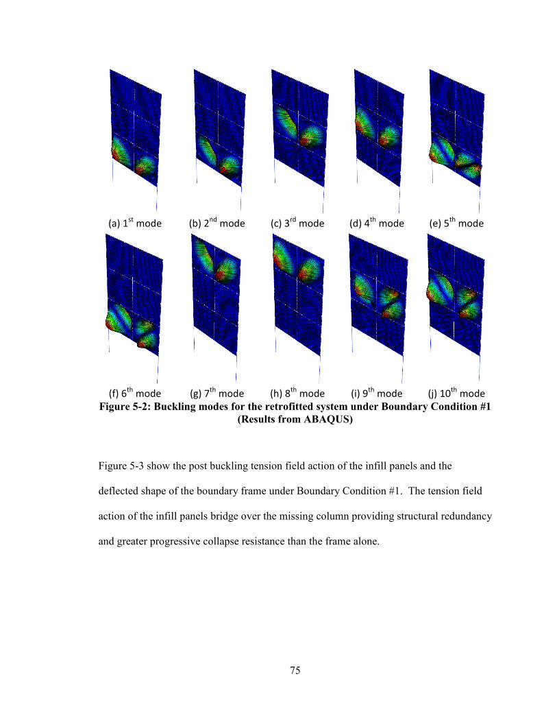
75
(a) 1
st mode
(b) 2
nd mode
(c) 3
rd mode
(d) 4
th mode
(e) 5
th mode
(f) 6
th mode
(g) 7
th mode
(h) 8
th mode
(i) 9
th mode
(j) 10
th mode
Figure 5-2: Buckling modes for the retrofitted system under Boundary Condition #1
(Results from ABAQUS)
Figure 5-3 show the post buckling tension field action of the infill panels and the
deflected shape of the boundary frame under Boundary Condition #1. The tension field
action of the infill panels bridge over the missing column providing structural redundancy
and greater progressive collapse resistance than the frame alone.
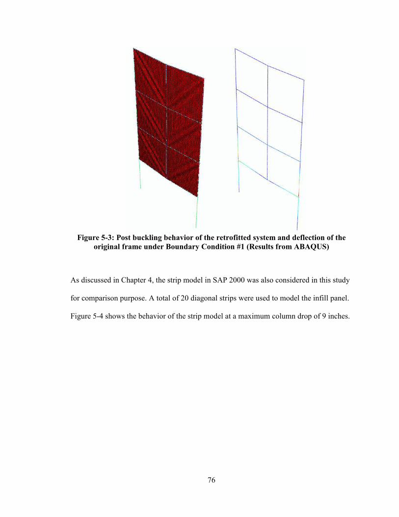
76
Figure 5-3: Post buckling behavior of the retrofitted system and deflection of the
original frame under Boundary Condition #1 (Results from ABAQUS)
As discussed in Chapter 4, the strip model in SAP 2000 was also considered in this study
for comparison purpose. A total of 20 diagonal strips were used to model the infill panel.
Figure 5-4 shows the behavior of the strip model at a maximum column drop of 9 inches.
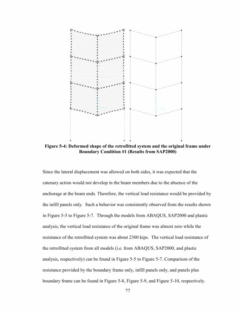
77
Figure 5-4: Deformed shape of the retrofitted system and the original frame under
Boundary Condition #1 (Results from SAP2000)
Since the lateral displacement was allowed on both sides, it was expected that the
catenary action would not develop in the beam members due to the absence of the
anchorage at the beam ends. Therefore, the vertical load resistance would be provided by
the infill panels only. Such a behavior was consistently observed from the results shown
in Figure 5-5 to Figure 5-7. Through the models from ABAQUS, SAP2000 and plastic
analysis, the vertical load resistance of the original frame was almost zero while the
resistance of the retrofitted system was about 2300 kips. The vertical load resistance of
the retrofitted system from all models (i.e. from ABAQUS, SAP2000, and plastic
analysis, respectively) can be found in Figure 5-5 to Figure 5-7. Comparison of the
resistance provided by the boundary frame only, infill panels only, and panels plus
boundary frame can be found in Figure 5-8, Figure 5-9, and Figure 5-10, respectively.
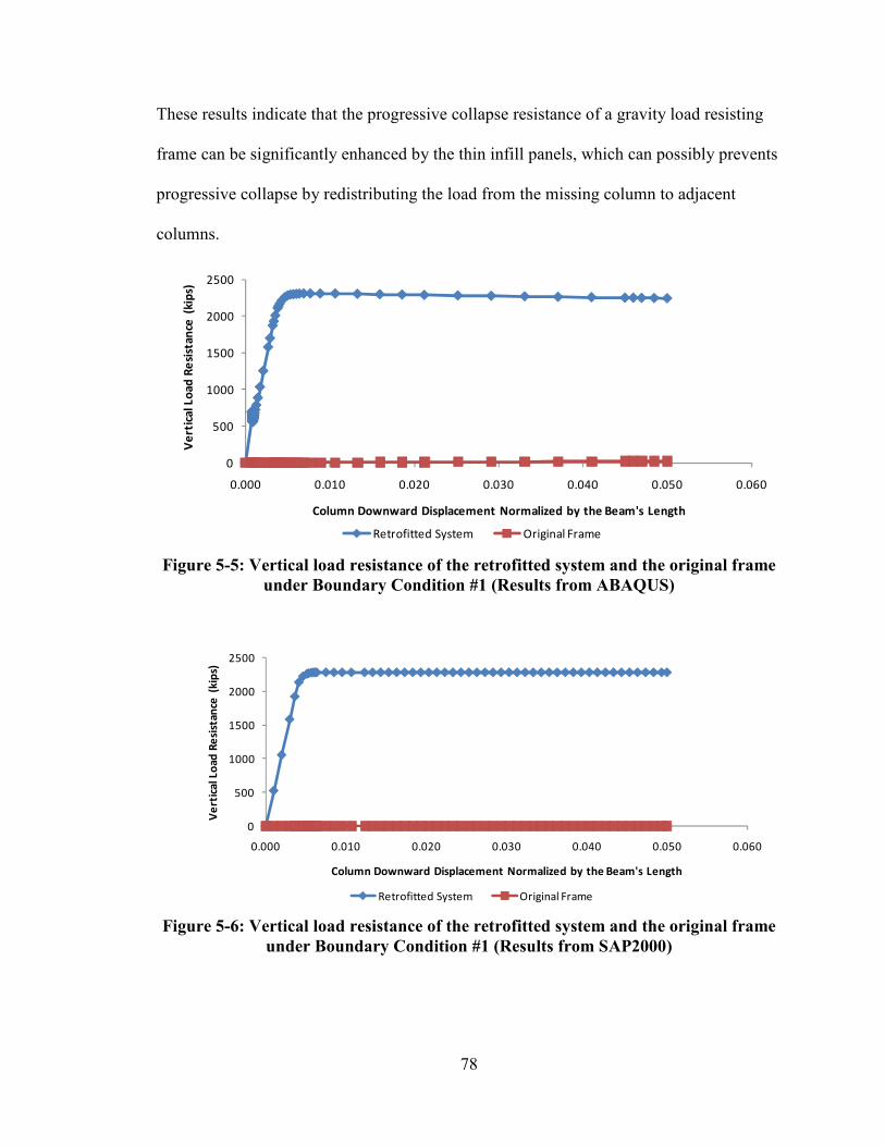
78
These results indicate that the progressive collapse resistance of a gravity load resisting
frame can be significantly enhanced by the thin infill panels, which can possibly prevents
progressive collapse by redistributing the load from the missing column to adjacent
columns.
Figure 5-5: Vertical load resistance of the retrofitted system and the original frame
under Boundary Condition #1 (Results from ABAQUS)
Figure 5-6: Vertical load resistance of the retrofitted system and the original frame
under Boundary Condition #1 (Results from SAP2000)
0
500
1000
1500
2000
2500
0.000 0.010 0.020 0.030 0.040 0.050 0.060
Ve
rtic
al
Lo
ad
Re
sist
an
ce (
kip
s)
Column Downward Displacement Normalized by the Beam's Length
Retrofitted System Original Frame
0
500
1000
1500
2000
2500
0.000 0.010 0.020 0.030 0.040 0.050 0.060
Ve
rtic
al
Lo
ad
Re
sist
an
ce (
kip
s)
Column Downward Displacement Normalized by the Beam's Length
Retrofitted System Original Frame
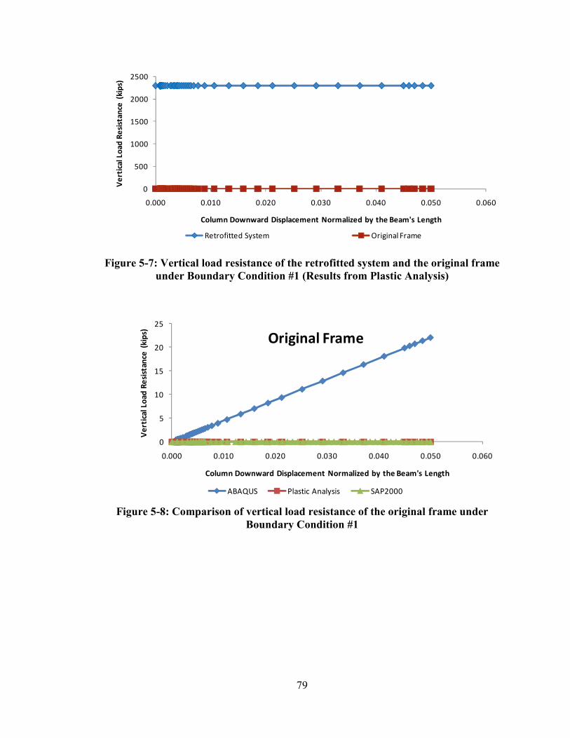
79
Figure 5-7: Vertical load resistance of the retrofitted system and the original frame
under Boundary Condition #1 (Results from Plastic Analysis)
Figure 5-8: Comparison of vertical load resistance of the original frame under
Boundary Condition #1
0
500
1000
1500
2000
2500
0.000 0.010 0.020 0.030 0.040 0.050 0.060
Ve
rtic
al
Lo
ad
Re
sist
an
ce (
kip
s)
Column Downward Displacement Normalized by the Beam's Length
Retrofitted System Original Frame
0
5
10
15
20
25
0.000 0.010 0.020 0.030 0.040 0.050 0.060
Ve
rtic
al
Lo
ad
Re
sist
an
ce (
kip
s)
Column Downward Displacement Normalized by the Beam's Length
Original Frame
ABAQUS Plastic Analysis SAP2000
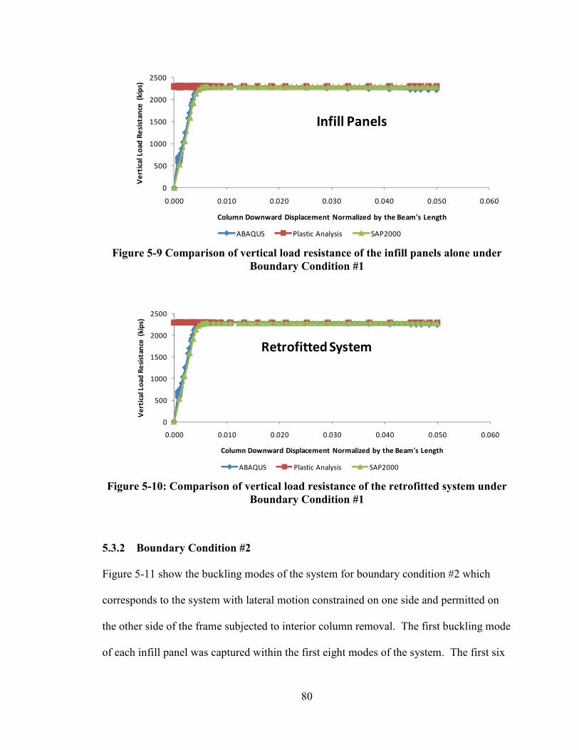
80
Figure 5-9 Comparison of vertical load resistance of the infill panels alone under
Boundary Condition #1
Figure 5-10: Comparison of vertical load resistance of the retrofitted system under
Boundary Condition #1
5.3.2 Boundary Condition #2
Figure 5-11 show the buckling modes of the system for boundary condition #2 which
corresponds to the system with lateral motion constrained on one side and permitted on
the other side of the frame subjected to interior column removal. The first buckling mode
of each infill panel was captured within the first eight modes of the system. The first six
0
500
1000
1500
2000
2500
0.000 0.010 0.020 0.030 0.040 0.050 0.060
Ve
rtic
al
Lo
ad
Re
sist
an
ce (
kip
s)
Column Downward Displacement Normalized by the Beam's Length
Infill Panels
ABAQUS Plastic Analysis SAP2000
0
500
1000
1500
2000
2500
0.000 0.010 0.020 0.030 0.040 0.050 0.060
Ve
rtic
al
Lo
ad
Re
sist
an
ce (
kip
s)
Column Downward Displacement Normalized by the Beam's Length
Retrofitted System
ABAQUS Plastic Analysis SAP2000
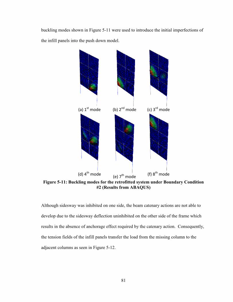
81
buckling modes shown in Figure 5-11 were used to introduce the initial imperfections of
the infill panels into the push down model.
(a) 1
st mode
(b) 2
nd mode
(c) 3
rd mode
(d) 4
th mode
(e) 7th
mode
(f) 8
th mode
Figure 5-11: Buckling modes for the retrofitted system under Boundary Condition
#2 (Results from ABAQUS)
Although sidesway was inhibited on one side, the beam catenary actions are not able to
develop due to the sidesway deflection uninhibited on the other side of the frame which
results in the absence of anchorage effect required by the catenary action. Consequently,
the tension fields of the infill panels transfer the load from the missing column to the
adjacent columns as seen in Figure 5-12.
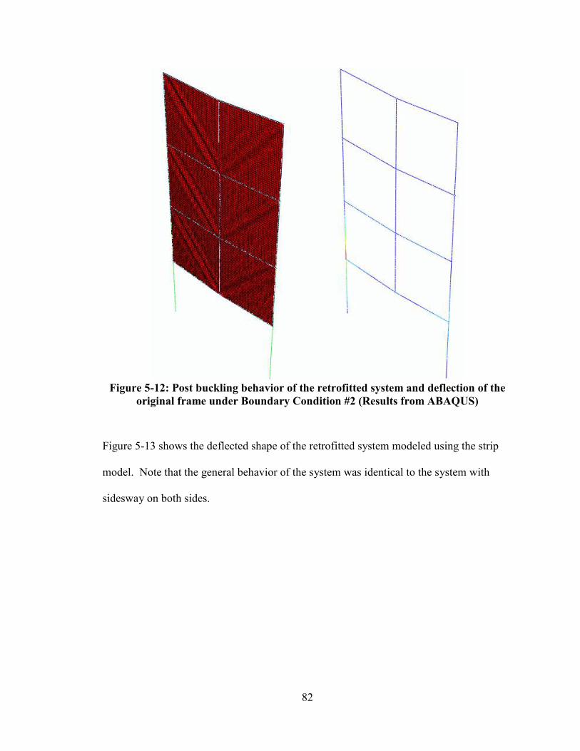
82
Figure 5-12: Post buckling behavior of the retrofitted system and deflection of the
original frame under Boundary Condition #2 (Results from ABAQUS)
Figure 5-13 shows the deflected shape of the retrofitted system modeled using the strip
model. Note that the general behavior of the system was identical to the system with
sidesway on both sides.
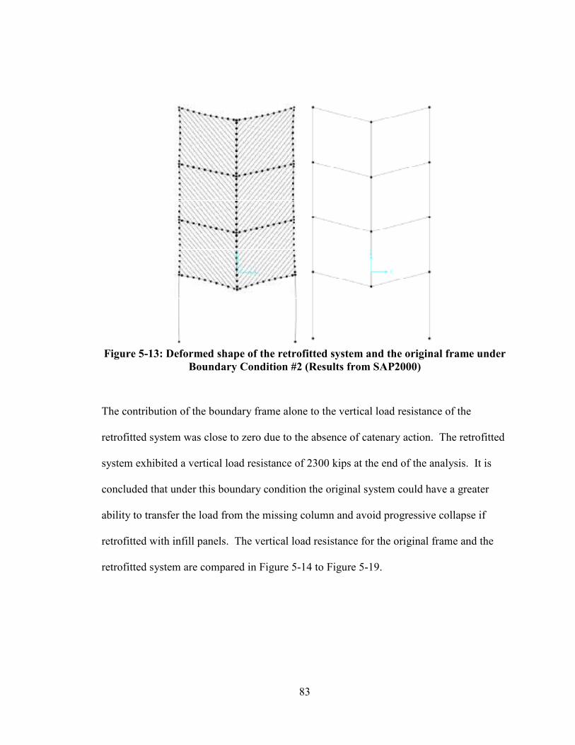
83
Figure 5-13: Deformed shape of the retrofitted system and the original frame under
Boundary Condition #2 (Results from SAP2000)
The contribution of the boundary frame alone to the vertical load resistance of the
retrofitted system was close to zero due to the absence of catenary action. The retrofitted
system exhibited a vertical load resistance of 2300 kips at the end of the analysis. It is
concluded that under this boundary condition the original system could have a greater
ability to transfer the load from the missing column and avoid progressive collapse if
retrofitted with infill panels. The vertical load resistance for the original frame and the
retrofitted system are compared in Figure 5-14 to Figure 5-19.
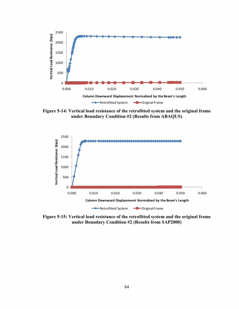
84
Figure 5-14: Vertical load resistance of the retrofitted system and the original frame
under Boundary Condition #2 (Results from ABAQUS)
Figure 5-15: Vertical load resistance of the retrofitted system and the original frame
under Boundary Condition #2 (Results from SAP2000)
0
500
1000
1500
2000
2500
0.000 0.010 0.020 0.030 0.040 0.050 0.060
Ve
rtic
al
Lo
ad
Re
sist
an
ce (
kip
s)
Column Downward Displacement Normalized by the Beam's Length
Retrofitted System Original Frame
0
500
1000
1500
2000
2500
0.000 0.010 0.020 0.030 0.040 0.050 0.060
Ve
rtic
al
Lo
ad
Re
sist
an
ce (
kip
s)
Column Downward Displacement Normalized by the Beam's Length
Retrofitted System Original Frame
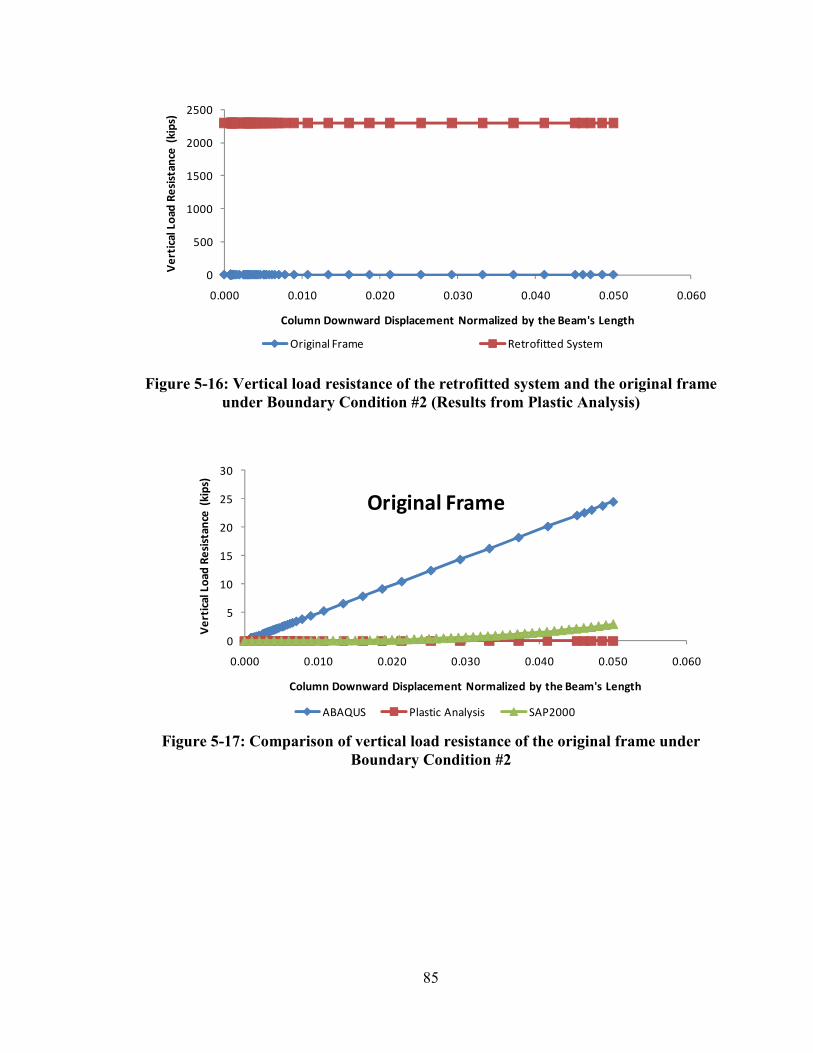
85
Figure 5-16: Vertical load resistance of the retrofitted system and the original frame
under Boundary Condition #2 (Results from Plastic Analysis)
Figure 5-17: Comparison of vertical load resistance of the original frame under
Boundary Condition #2
0
500
1000
1500
2000
2500
0.000 0.010 0.020 0.030 0.040 0.050 0.060
Ve
rtic
al
Lo
ad
Re
sist
an
ce (
kip
s)
Column Downward Displacement Normalized by the Beam's Length
Original Frame Retrofitted System
0
5
10
15
20
25
30
0.000 0.010 0.020 0.030 0.040 0.050 0.060
Ve
rtic
al
Lo
ad
Re
sist
an
ce (
kip
s)
Column Downward Displacement Normalized by the Beam's Length
Original Frame
ABAQUS Plastic Analysis SAP2000
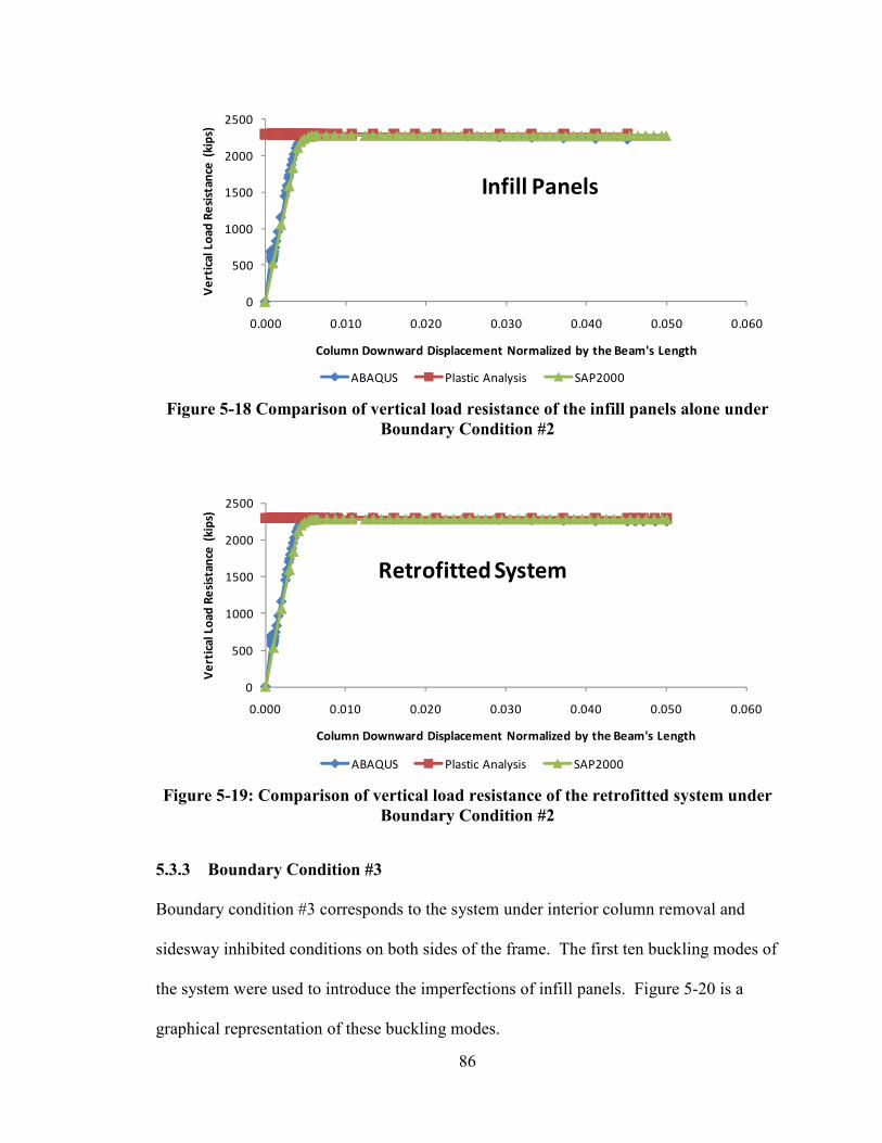
86
Figure 5-18 Comparison of vertical load resistance of the infill panels alone under
Boundary Condition #2
Figure 5-19: Comparison of vertical load resistance of the retrofitted system under
Boundary Condition #2
5.3.3 Boundary Condition #3
Boundary condition #3 corresponds to the system under interior column removal and
sidesway inhibited conditions on both sides of the frame. The first ten buckling modes of
the system were used to introduce the imperfections of infill panels. Figure 5-20 is a
graphical representation of these buckling modes.
0
500
1000
1500
2000
2500
0.000 0.010 0.020 0.030 0.040 0.050 0.060
Ve
rtic
al
Lo
ad
Re
sist
an
ce (
kip
s)
Column Downward Displacement Normalized by the Beam's Length
Infill Panels
ABAQUS Plastic Analysis SAP2000
0
500
1000
1500
2000
2500
0.000 0.010 0.020 0.030 0.040 0.050 0.060
Ve
rtic
al
Lo
ad
Re
sist
an
ce (
kip
s)
Column Downward Displacement Normalized by the Beam's Length
Retrofitted System
ABAQUS Plastic Analysis SAP2000
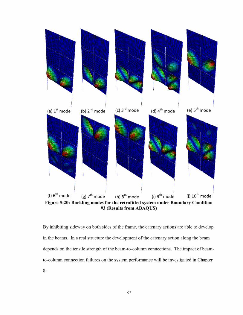
87
(a) 1st
mode (b) 2nd
mode (c) 3rd
mode (d) 4th
mode (e) 5th
mode
(f) 6th
mode (g) 7th
mode (h) 8th
mode
(i) 9th
mode (j) 10th
mode
Figure 5-20: Buckling modes for the retrofitted system under Boundary Condition
#3 (Results from ABAQUS)
By inhibiting sideway on both sides of the frame, the catenary actions are able to develop
in the beams. In a real structure the development of the catenary action along the beam
depends on the tensile strength of the beam-to-column connections. The impact of beam-
to-column connection failures on the system performance will be investigated in Chapter
8.
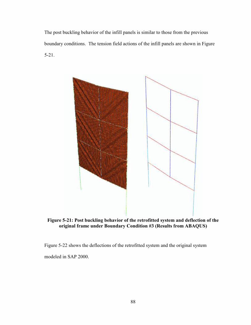
88
The post buckling behavior of the infill panels is similar to those from the previous
boundary conditions. The tension field actions of the infill panels are shown in Figure
5-21.
Figure 5-21: Post buckling behavior of the retrofitted system and deflection of the
original frame under Boundary Condition #3 (Results from ABAQUS)
Figure 5-22 shows the deflections of the retrofitted system and the original system
modeled in SAP 2000.
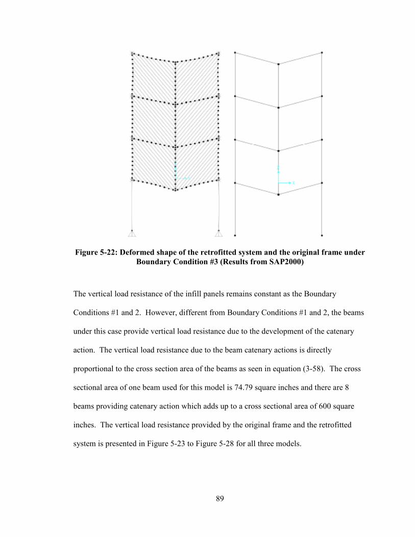
89
Figure 5-22: Deformed shape of the retrofitted system and the original frame under
Boundary Condition #3 (Results from SAP2000)
The vertical load resistance of the infill panels remains constant as the Boundary
Conditions #1 and 2. However, different from Boundary Conditions #1 and 2, the beams
under this case provide vertical load resistance due to the development of the catenary
action. The vertical load resistance due to the beam catenary actions is directly
proportional to the cross section area of the beams as seen in equation (3-58). The cross
sectional area of one beam used for this model is 74.79 square inches and there are 8
beams providing catenary action which adds up to a cross sectional area of 600 square
inches. The vertical load resistance provided by the original frame and the retrofitted
system is presented in Figure 5-23 to Figure 5-28 for all three models.
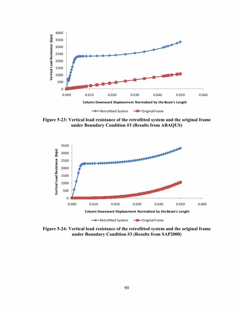
90
Figure 5-23: Vertical load resistance of the retrofitted system and the original frame
under Boundary Condition #3 (Results from ABAQUS)
Figure 5-24: Vertical load resistance of the retrofitted system and the original frame
under Boundary Condition #3 (Results from SAP2000)
0
500
1000
1500
2000
2500
3000
3500
4000
0.000 0.010 0.020 0.030 0.040 0.050 0.060
Ve
rtic
al
Lo
ad
Re
sist
an
ce (
kip
s)
Column Downward Displacement Normalized by the Beam's Length
Retrofitted System Original Frame
0
500
1000
1500
2000
2500
3000
3500
0.000 0.010 0.020 0.030 0.040 0.050 0.060
Ve
rtic
al
Lo
ad
Re
sist
an
ce (
kip
s)
Column Downward Displacement Normalized by the Beam's Length
Retrofitted System Original Frame
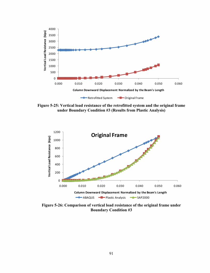
91
Figure 5-25: Vertical load resistance of the retrofitted system and the original frame
under Boundary Condition #3 (Results from Plastic Analysis)
Figure 5-26: Comparison of vertical load resistance of the original frame under
Boundary Condition #3
0
500
1000
1500
2000
2500
3000
3500
4000
0.000 0.010 0.020 0.030 0.040 0.050 0.060
Ve
rtic
al
Lo
ad
Re
sist
an
ce (
kip
s)
Column Downward Displacement Normalized by the Beam's Length
Retrofitted System Original Frame
0
200
400
600
800
1000
1200
0.000 0.010 0.020 0.030 0.040 0.050 0.060
Ve
rtic
al
Lo
ad
Re
sist
an
ce (
kip
s)
Column Downward Displacement Normalized by the Beam's Length
Original Frame
ABAQUS Plastic Analysis SAP2000
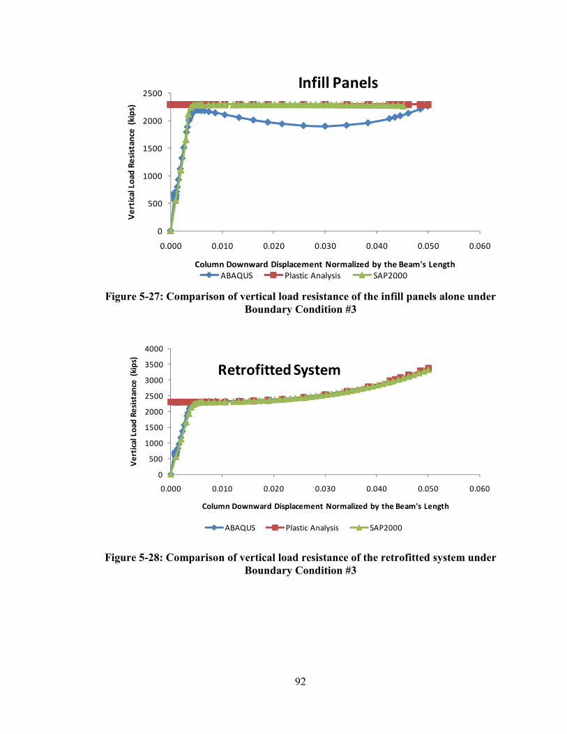
92
Figure 5-27: Comparison of vertical load resistance of the infill panels alone under
Boundary Condition #3
Figure 5-28: Comparison of vertical load resistance of the retrofitted system under
Boundary Condition #3
0
500
1000
1500
2000
2500
0.000 0.010 0.020 0.030 0.040 0.050 0.060
Ve
rtic
al
Lo
ad
Re
sist
an
ce (
kip
s)
Column Downward Displacement Normalized by the Beam's Length
Infill Panels
ABAQUS Plastic Analysis SAP2000
0
500
1000
1500
2000
2500
3000
3500
4000
0.000 0.010 0.020 0.030 0.040 0.050 0.060
Ve
rtic
al
Lo
ad
Re
sist
an
ce (
kip
s)
Column Downward Displacement Normalized by the Beam's Length
Retrofitted System
ABAQUS Plastic Analysis SAP2000
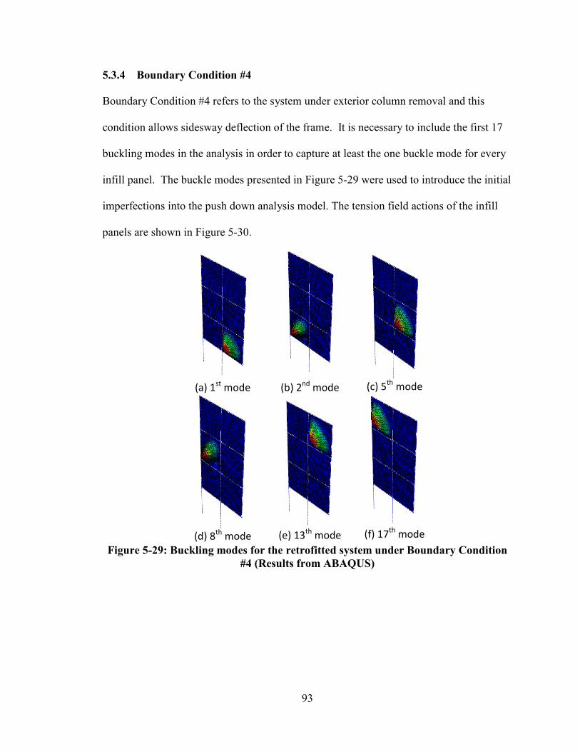
93
5.3.4 Boundary Condition #4
Boundary Condition #4 refers to the system under exterior column removal and this
condition allows sidesway deflection of the frame. It is necessary to include the first 17
buckling modes in the analysis in order to capture at least the one buckle mode for every
infill panel. The buckle modes presented in Figure 5-29 were used to introduce the initial
imperfections into the push down analysis model. The tension field actions of the infill
panels are shown in Figure 5-30.
(a) 1
st mode
(b) 2
nd mode
(c) 5
th mode
(d) 8
th mode
(e) 13
th mode
(f) 17
th mode
Figure 5-29: Buckling modes for the retrofitted system under Boundary Condition
#4 (Results from ABAQUS)
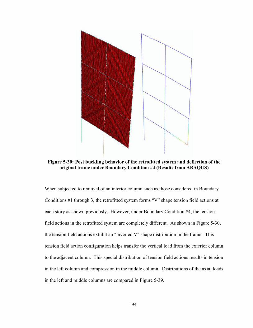
94
Figure 5-30: Post buckling behavior of the retrofitted system and deflection of the
original frame under Boundary Condition #4 (Results from ABAQUS)
When subjected to removal of an interior column such as those considered in Boundary
Conditions #1 through 3, the retrofitted system forms “V” shape tension field actions at
each story as shown previously. However, under Boundary Condition #4, the tension
field actions in the retrofitted system are completely different. As shown in Figure 5-30,
the tension field actions exhibit an "inverted V" shape distribution in the frame. This
tension field action configuration helps transfer the vertical load from the exterior column
to the adjacent column. This special distribution of tension field actions results in tension
in the left column and compression in the middle column. Distributions of the axial loads
in the left and middle columns are compared in Figure 5-39.
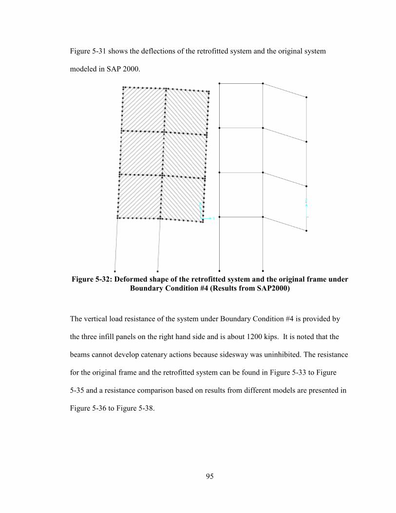
95
Figure 5-31 shows the deflections of the retrofitted system and the original system
modeled in SAP 2000.
Figure 5-32: Deformed shape of the retrofitted system and the original frame under
Boundary Condition #4 (Results from SAP2000)
The vertical load resistance of the system under Boundary Condition #4 is provided by
the three infill panels on the right hand side and is about 1200 kips. It is noted that the
beams cannot develop catenary actions because sidesway was uninhibited. The resistance
for the original frame and the retrofitted system can be found in Figure 5-33 to Figure
5-35 and a resistance comparison based on results from different models are presented in
Figure 5-36 to Figure 5-38.
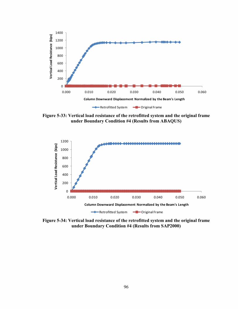
96
Figure 5-33: Vertical load resistance of the retrofitted system and the original frame
under Boundary Condition #4 (Results from ABAQUS)
Figure 5-34: Vertical load resistance of the retrofitted system and the original frame
under Boundary Condition #4 (Results from SAP2000)
0
200
400
600
800
1000
1200
1400
0.000 0.010 0.020 0.030 0.040 0.050 0.060
Ve
rtic
al
Lo
ad
Re
sist
an
ce (
kip
s)
Column Downward Displacement Normalized by the Beam's Length
Retrofitted System Original Frame
0
200
400
600
800
1000
1200
0.000 0.010 0.020 0.030 0.040 0.050 0.060
Ve
rtic
al
Lo
ad
Re
sist
an
ce (
kip
s)
Column Downward Displacement Normalized by the Beam's Length
Retrofitted System Original Frame

97
Figure 5-35: Vertical load resistance of the retrofitted system and the original frame
under Boundary Condition #4 (Results from Plastic Analysis))
Figure 5-36: Comparison of vertical load resistance of the original frame under
Boundary Condition #4
0
200
400
600
800
1000
1200
1400
0.000 0.010 0.020 0.030 0.040 0.050 0.060
Ve
rtic
al
Lo
ad
Re
sist
an
ce (
kip
s)
Column Downward Displacement Normalized by the Beam's Length
Retrofitted System Original Frame
0
2
4
6
8
10
12
0.000 0.010 0.020 0.030 0.040 0.050 0.060
Ve
rtic
al
Lo
ad
Re
sist
an
ce (
kip
s)
Column Downward Displacement Normalized by the Beam's Length
Original Frame
ABAQUS Plastic Analysis SAP2000

98
Figure 5-37: Comparison of vertical load resistance of the infill panels alone under
Boundary Condition #4
Figure 5-38: Comparison of vertical load resistance of the retrofitted system under
Boundary Condition #4
0
200
400
600
800
1000
1200
1400
0.000 0.010 0.020 0.030 0.040 0.050 0.060
Ve
rtic
al
Lo
ad
Re
sist
an
ce (
kip
s)
Column Downward Displacement Normalized by the Beam's Length
Infill Panels
ABAQUS Plastic Analysis SAP2000
0
200
400
600
800
1000
1200
1400
0.000 0.010 0.020 0.030 0.040 0.050 0.060
Ve
rtic
al
Lo
ad
Re
sist
an
ce (
kip
s)
Column Downward Displacement Normalized by the Beam's Length
Retrofitted System
ABAQUS Plastic Analysis SAP2000
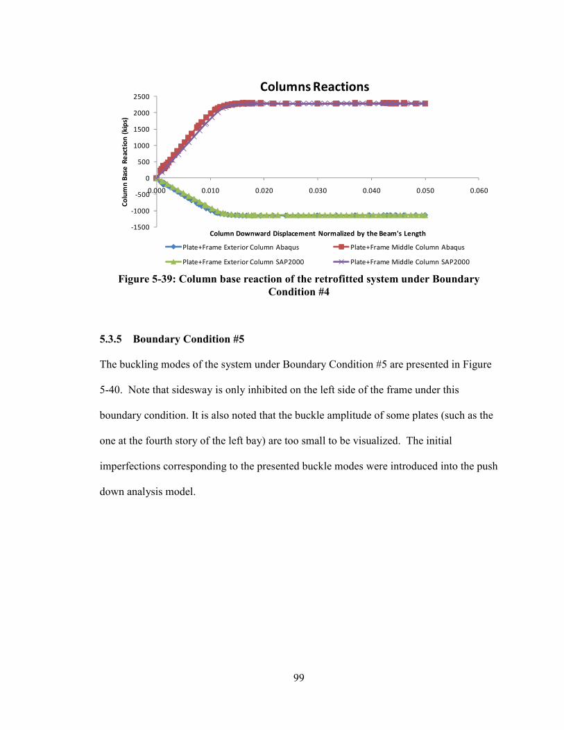
99
Figure 5-39: Column base reaction of the retrofitted system under Boundary
Condition #4
5.3.5 Boundary Condition #5
The buckling modes of the system under Boundary Condition #5 are presented in Figure
5-40. Note that sidesway is only inhibited on the left side of the frame under this
boundary condition. It is also noted that the buckle amplitude of some plates (such as the
one at the fourth story of the left bay) are too small to be visualized. The initial
imperfections corresponding to the presented buckle modes were introduced into the push
down analysis model.
-1500
-1000
-500
0
500
1000
1500
2000
2500
0.000 0.010 0.020 0.030 0.040 0.050 0.060
Co
lum
n B
ase
Re
act
ion
(k
ips)
Column Downward Displacement Normalized by the Beam's Length
Columns Reactions
Plate+Frame Exterior Column Abaqus Plate+Frame Middle Column Abaqus
Plate+Frame Exterior Column SAP2000 Plate+Frame Middle Column SAP2000
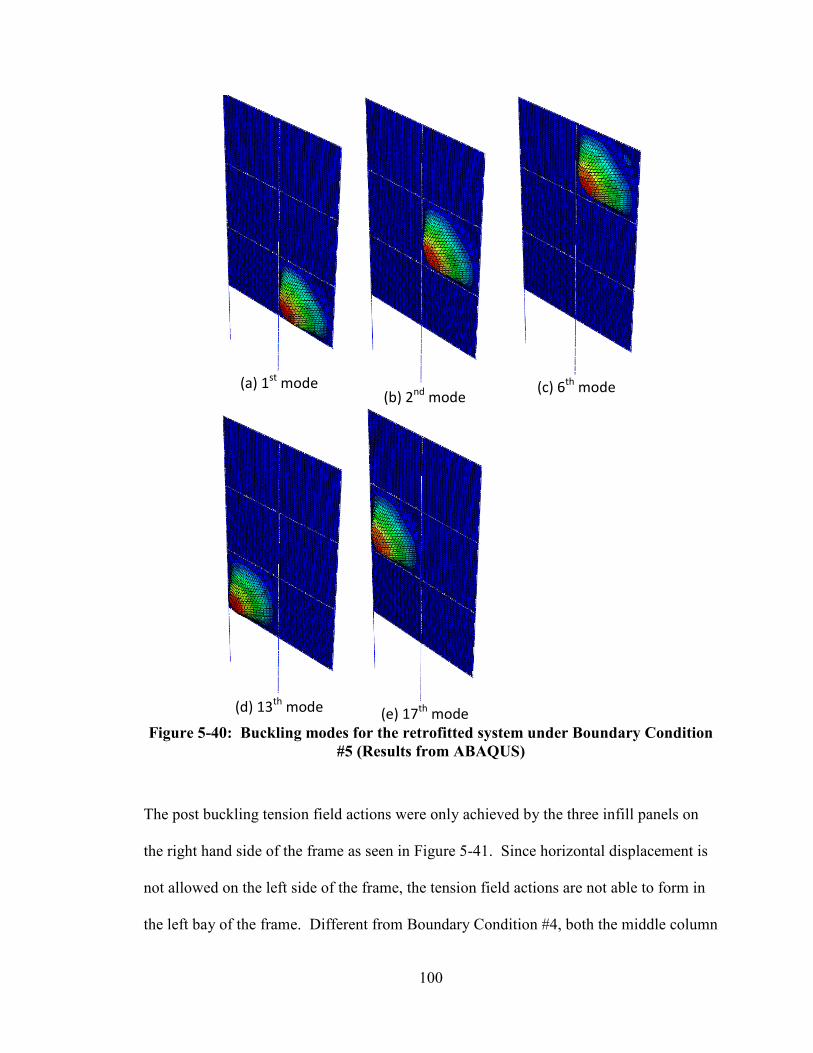
100
(a) 1
st mode
(b) 2nd
mode
(c) 6
th mode
(d) 13
th mode
(e) 17
th mode
Figure 5-40: Buckling modes for the retrofitted system under Boundary Condition
#5 (Results from ABAQUS)
The post buckling tension field actions were only achieved by the three infill panels on
the right hand side of the frame as seen in Figure 5-41. Since horizontal displacement is
not allowed on the left side of the frame, the tension field actions are not able to form in
the left bay of the frame. Different from Boundary Condition #4, both the middle column
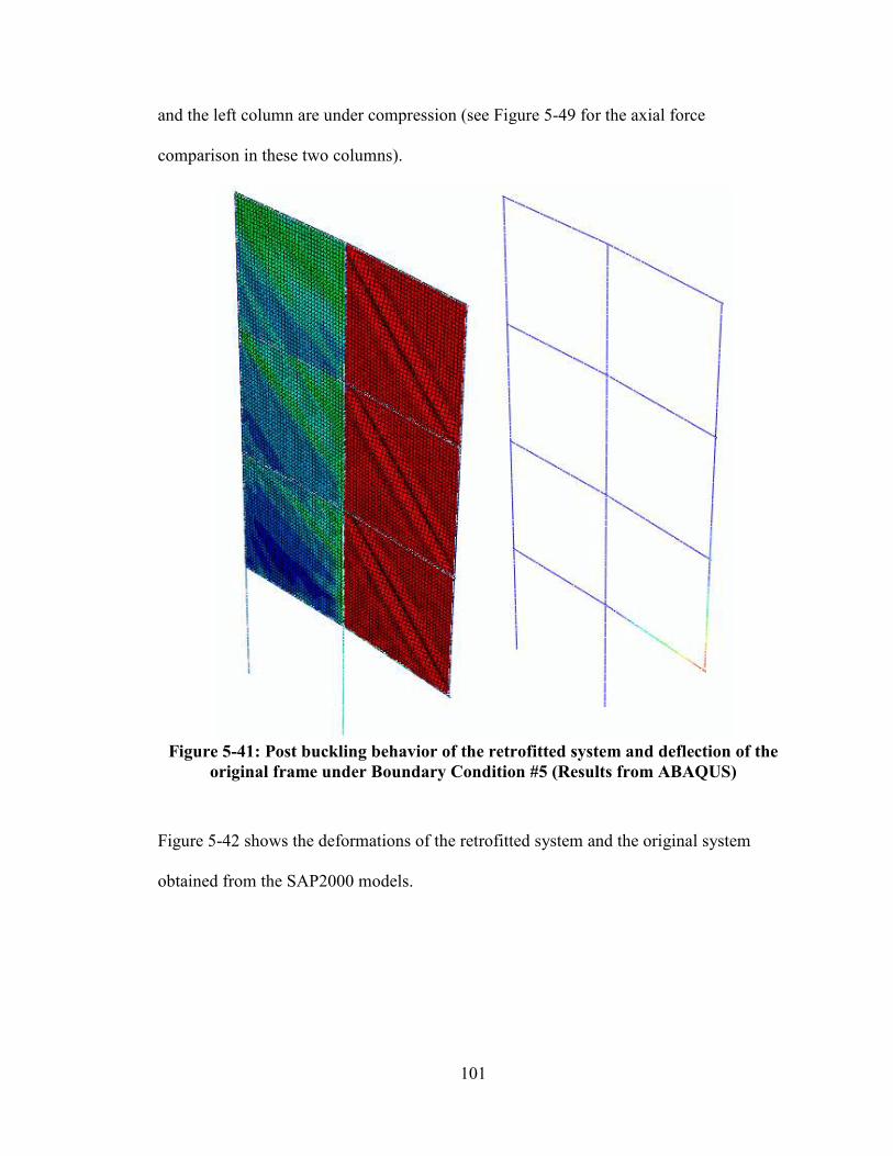
101
and the left column are under compression (see Figure 5-49 for the axial force
comparison in these two columns).
Figure 5-41: Post buckling behavior of the retrofitted system and deflection of the
original frame under Boundary Condition #5 (Results from ABAQUS)
Figure 5-42 shows the deformations of the retrofitted system and the original system
obtained from the SAP2000 models.

102
Figure 5-42: Deformed shape of the retrofitted system and the original frame under
Boundary Condition #5 (Results from SAP2000)
Comparing the results from Boundary Conditions #4 and 5, it is observed that the vertical
load resistances are identical to 1200 kips in both cases due to the same tension field
action distributions in the right bay of the frame. Moreover, the beams cannot develop
catenary actions either. The resistance for the original frame and the retrofitted system
can be found in Figure 5-33 to Figure 5-35 and a resistance comparison based on results
from different models are presented in Figure 5-36 to Figure 5-38.
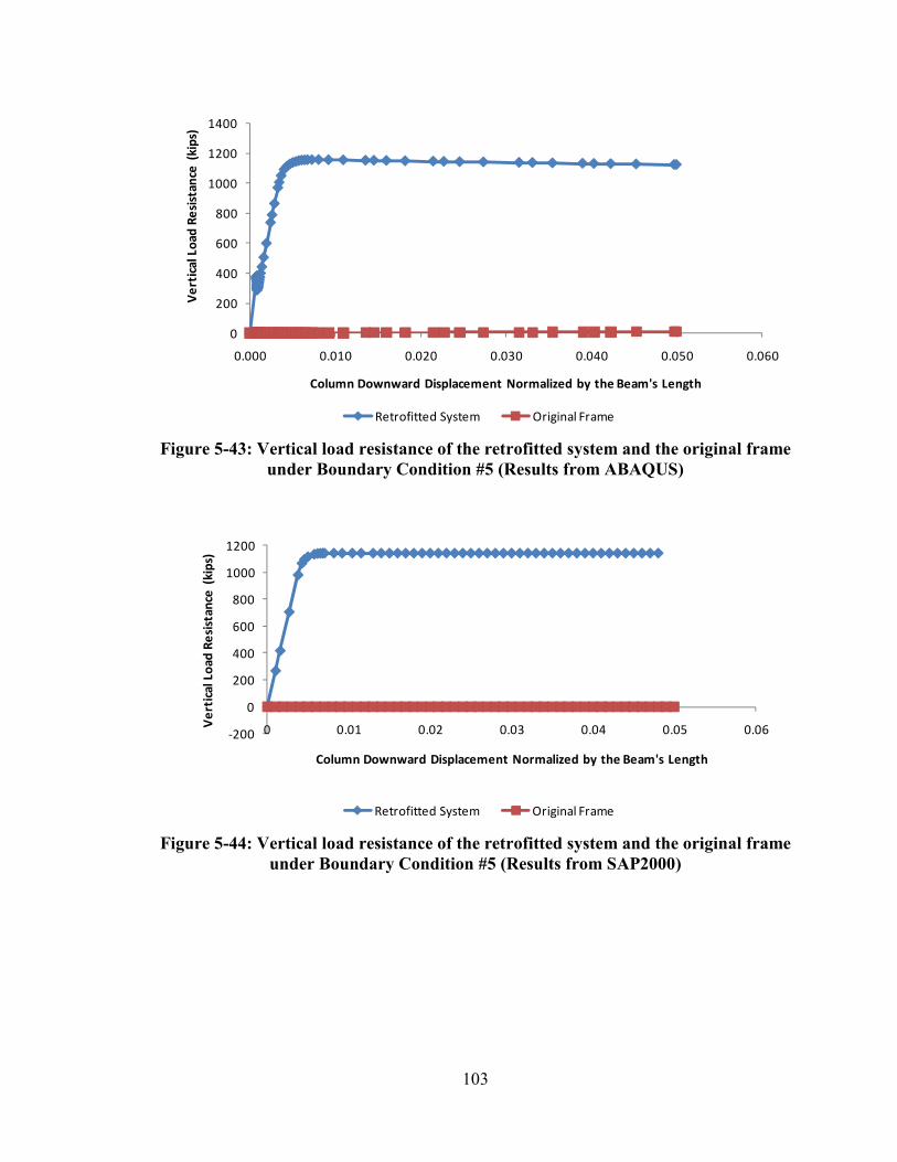
103
Figure 5-43: Vertical load resistance of the retrofitted system and the original frame
under Boundary Condition #5 (Results from ABAQUS)
Figure 5-44: Vertical load resistance of the retrofitted system and the original frame
under Boundary Condition #5 (Results from SAP2000)
0
200
400
600
800
1000
1200
1400
0.000 0.010 0.020 0.030 0.040 0.050 0.060
Ve
rtic
al
Lo
ad
Re
sist
an
ce (
kip
s)
Column Downward Displacement Normalized by the Beam's Length
Retrofitted System Original Frame
-200
0
200
400
600
800
1000
1200
0 0.01 0.02 0.03 0.04 0.05 0.06
Ve
rtic
al
Lo
ad
Re
sist
an
ce (
kip
s)
Column Downward Displacement Normalized by the Beam's Length
Retrofitted System Original Frame

104
Figure 5-45: Vertical load resistance of the retrofitted system and the original frame
under Boundary Condition #5 (Results from Plastic Analysis)
Figure 5-46: Comparison of vertical load resistance of the original frame under
Boundary Condition #5
0
200
400
600
800
1000
1200
1400
0.000 0.010 0.020 0.030 0.040 0.050 0.060
Ve
rtic
al
Lo
ad
Re
sist
an
ce (
kip
s)
Column Downward Displacement Normalized by the Beam's Length
Platic analysis
Retrofitted System Original Frame
-2
0
2
4
6
8
10
12
0.000 0.010 0.020 0.030 0.040 0.050 0.060Ve
rtic
al
Lo
ad
Re
sist
an
ce (
kip
s)
Column Downward Displacement Normalized by the Beam's Length
Original Frame
ABAQUS Plastic Analysis SAP2000
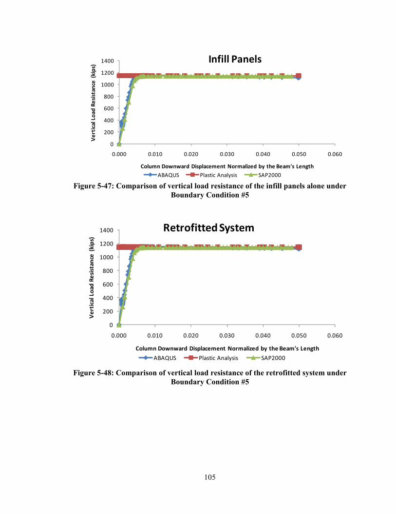
105
Figure 5-47: Comparison of vertical load resistance of the infill panels alone under
Boundary Condition #5
Figure 5-48: Comparison of vertical load resistance of the retrofitted system under
Boundary Condition #5
0
200
400
600
800
1000
1200
1400
0.000 0.010 0.020 0.030 0.040 0.050 0.060
Ve
rtic
al
Lo
ad
Re
sist
an
ce (
kip
s)
Column Downward Displacement Normalized by the Beam's Length
Infill Panels
ABAQUS Plastic Analysis SAP2000
0
200
400
600
800
1000
1200
1400
0.000 0.010 0.020 0.030 0.040 0.050 0.060
Ve
rtic
al
Lo
ad
Re
sist
an
ce (
kip
s)
Column Downward Displacement Normalized by the Beam's Length
Retrofitted System
ABAQUS Plastic Analysis SAP2000
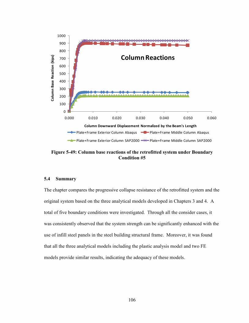
106
Figure 5-49: Column base reactions of the retrofitted system under Boundary
Condition #5
5.4 Summary
The chapter compares the progressive collapse resistance of the retrofitted system and the
original system based on the three analytical models developed in Chapters 3 and 4. A
total of five boundary conditions were investigated. Through all the consider cases, it
was consistently observed that the system strength can be significantly enhanced with the
use of infill steel panels in the steel building structural frame. Moreover, it was found
that all the three analytical models including the plastic analysis model and two FE
models provide similar results, indicating the adequacy of these models.
0
100
200
300
400
500
600
700
800
900
1000
0.000 0.010 0.020 0.030 0.040 0.050 0.060
Co
lum
n B
ase
Re
act
ion
(k
ips)
Column Downward Displacement Normalized by the Beam's Length
Column Reactions
Plate+Frame Exterior Column Abaqus Plate+Frame Middle Column Abaqus
Plate+Frame Exterior Column SAP2000 Plate+Frame Middle Column SAP2000
107
6 PSEUDO-STATIC RESPONSE OF THE PROPOSED SYSTEM
6.1 Introduction
As mentioned previously, the FE models presented in this thesis assume the threat of a
single column failure and these models were investigated using the nonlinear static
analysis procedure. As such, the nonlinear dynamic effects which may exist in the
system were not considered in the analysis. When a sudden column failure occurs,
building structures may exhibit highly nonlinear dynamic response due to the
gravitational acceleration. While conducting the nonlinear dynamic analysis on the
developed FE models is likely to provide a more accurate estimate of the system
performance, it is overly complicated and may not be convenient for practical
applications. Alternatively, UFC allows using a so-called dynamic increase factor (DIF)
to modify the structural resistance obtained from static analyses to get the dynamic
response. According to the UFC document (DoD 2009), a constant DIF of 2 should be
used for modifying the results from linear elastic analysis. The DoD provide a more
complex equation to determine the DIF for responses acquired using nonlinear static
analysis. It was determined that most steel frames should considered a DIF value of 1.3
and 1.5 (Marchand & Alfawakhiri, 2004). Given that the dynamic effects of the
proposed system may be different from conventional systems, the DIF values
recommended by the UFC may not be proper for modifying the performance of the
proposed system. As such, this chapter evaluates the DIF values for the proposed system
based on an approach developed by Izzuddin et al. (2007).
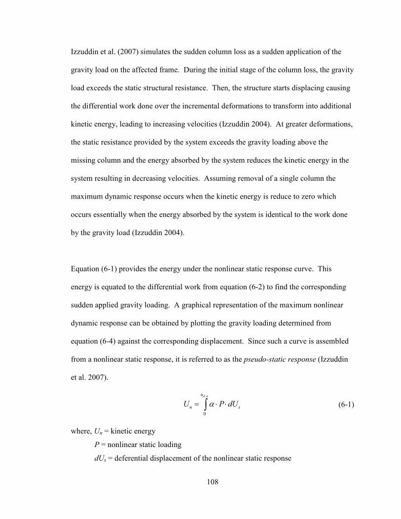
108
Izzuddin et al. (2007) simulates the sudden column loss as a sudden application of the
gravity load on the affected frame. During the initial stage of the column loss, the gravity
load exceeds the static structural resistance. Then, the structure starts displacing causing
the differential work done over the incremental deformations to transform into additional
kinetic energy, leading to increasing velocities (Izzuddin 2004). At greater deformations,
the static resistance provided by the system exceeds the gravity loading above the
missing column and the energy absorbed by the system reduces the kinetic energy in the
system resulting in decreasing velocities. Assuming removal of a single column the
maximum dynamic response occurs when the kinetic energy is reduce to zero which
occurs essentially when the energy absorbed by the system is identical to the work done
by the gravity load (Izzuddin 2004).
Equation (6-1) provides the energy under the nonlinear static response curve. This
energy is equated to the differential work from equation (6-2) to find the corresponding
sudden applied gravity loading. A graphical representation of the maximum nonlinear
dynamic response can be obtained by plotting the gravity loading determined from
equation (6-4) against the corresponding displacement. Since such a curve is assembled
from a nonlinear static response, it is referred to as the pseudo-static response (Izzuddin
et al. 2007).
,
0
d nu
n sU P dUα= ⋅ ⋅∫ (6-1)
where, Un = kinetic energy
P = nonlinear static loading
dUs = deferential displacement of the nonlinear static response
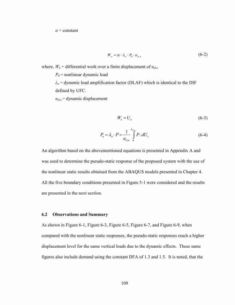
109
α = constant
0 ,n n d nW P uα λ= ⋅ ⋅ ⋅ (6-2)
where, Wn = differential work over a finite displacement of ud,n
P0 = nonlinear dynamic load
λn = dynamic load amplification factor (DLAF) which is identical to the DIF
defined by UFC.
ud,n = dynamic displacement
n nW U= (6-3)
,
, 0
1d nu
n n s
d n
P P P dUu
λ= ⋅ = ⋅∫ (6-4)
An algorithm based on the abovementioned equations is presented in Appendix A and
was used to determine the pseudo-static response of the proposed system with the use of
the nonlinear static results obtained from the ABAQUS models presented in Chapter 4.
All the five boundary conditions presented in Figure 5-1 were considered and the results
are presented in the next section.
6.2 Observations and Summary
As shown in Figure 6-1, Figure 6-3, Figure 6-5, Figure 6-7, and Figure 6-9, when
compared with the nonlinear static responses, the pseudo-static responses reach a higher
displacement level for the same vertical loads due to the dynamic effects. These same
figures also include demand using the constant DFA of 1.3 and 1.5. It is noted, that the
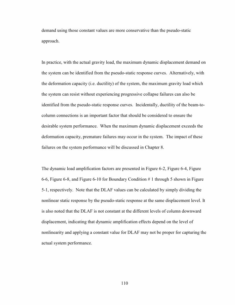
110
demand using those constant values are more conservative than the pseudo-static
approach.
In practice, with the actual gravity load, the maximum dynamic displacement demand on
the system can be identified from the pseudo-static response curves. Alternatively, with
the deformation capacity (i.e. ductility) of the system, the maximum gravity load which
the system can resist without experiencing progressive collapse failures can also be
identified from the pseudo-static response curves. Incidentally, ductility of the beam-to-
column connections is an important factor that should be considered to ensure the
desirable system performance. When the maximum dynamic displacement exceeds the
deformation capacity, premature failures may occur in the system. The impact of these
failures on the system performance will be discussed in Chapter 8.
The dynamic load amplification factors are presented in Figure 6-2, Figure 6-4, Figure
6-6, Figure 6-8, and Figure 6-10 for Boundary Condition # 1 through 5 shown in Figure
5-1, respectively. Note that the DLAF values can be calculated by simply dividing the
nonlinear static response by the pseudo-static response at the same displacement level. It
is also noted that the DLAF is not constant at the different levels of column downward
displacement, indicating that dynamic amplification effects depend on the level of
nonlinearity and applying a constant value for DLAF may not be proper for capturing the
actual system performance.
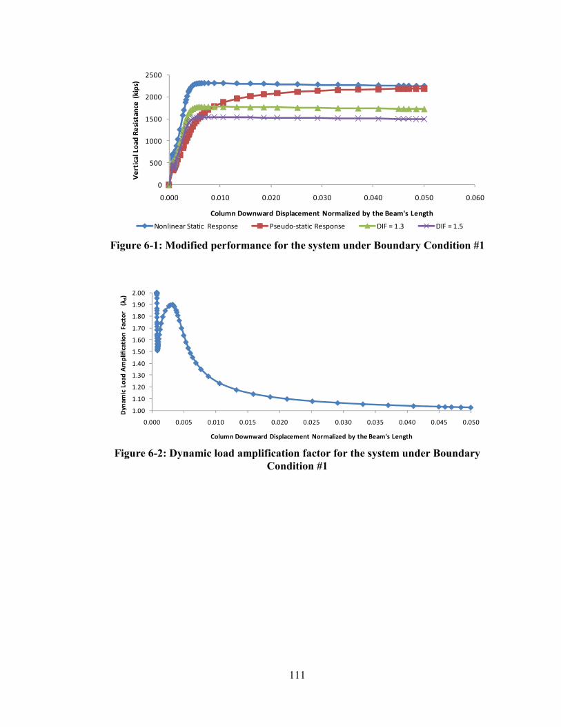
111
Figure 6-1: Modified performance for the system under Boundary Condition #1
Figure 6-2: Dynamic load amplification factor for the system under Boundary
Condition #1
0
500
1000
1500
2000
2500
0.000 0.010 0.020 0.030 0.040 0.050 0.060
Ve
rtic
al
Lo
ad
Re
sist
an
ce (
kip
s)
Column Downward Displacement Normalized by the Beam's Length
Nonlinear Static Response Pseudo-static Response DIF = 1.3 DIF = 1.5
1.00
1.10
1.20
1.30
1.40
1.50
1.60
1.70
1.80
1.90
2.00
0.000 0.005 0.010 0.015 0.020 0.025 0.030 0.035 0.040 0.045 0.050
Dy
na
mic
Lo
ad
Am
pli
fica
tio
n F
act
or
(λ
d)
Column Downward Displacement Normalized by the Beam's Length
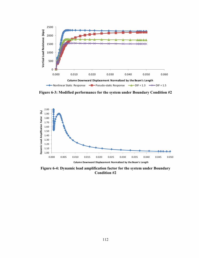
112
Figure 6-3: Modified performance for the system under Boundary Condition #2
Figure 6-4: Dynamic load amplification factor for the system under Boundary
Condition #2
0
500
1000
1500
2000
2500
0.000 0.010 0.020 0.030 0.040 0.050 0.060
Ve
rtic
al
Lo
ad
Re
sist
an
ce (
kip
s)
Column Downward Displacement Normalized by the Beam's Length
Nonlinear Static Response Pseudo-static Response DIF = 1.3 DIF = 1.5
1.00
1.10
1.20
1.30
1.40
1.50
1.60
1.70
1.80
1.90
2.00
0.000 0.005 0.010 0.015 0.020 0.025 0.030 0.035 0.040 0.045 0.050
Dy
na
mic
Lo
ad
Am
pli
fica
tio
n F
act
or
(λ
d)
Column Downward Displacement Normalized by the Beam's Length

113
Figure 6-5: Modified performance for the system under Boundary Condition #3
Figure 6-6: Dynamic load amplification factor for the system under Boundary
Condition #3
0
500
1000
1500
2000
2500
3000
3500
4000
0.000 0.010 0.020 0.030 0.040 0.050 0.060
Ve
rtic
al L
oa
d R
esi
stan
ce (
kip
s)
Column Downward Displacement Normalized by the Beam's Length
Nonlinear Static Response Pseudo-static Response DIF = 1.3 DIF = 1.5
1.00
1.10
1.20
1.30
1.40
1.50
1.60
1.70
1.80
1.90
2.00
0.000 0.005 0.010 0.015 0.020 0.025 0.030 0.035 0.040 0.045 0.050
Dy
na
mic
Lo
ad
Am
pli
fica
tio
n F
act
or
(λ
d)
Column Downward Displacement Normalized by the Beam's Length
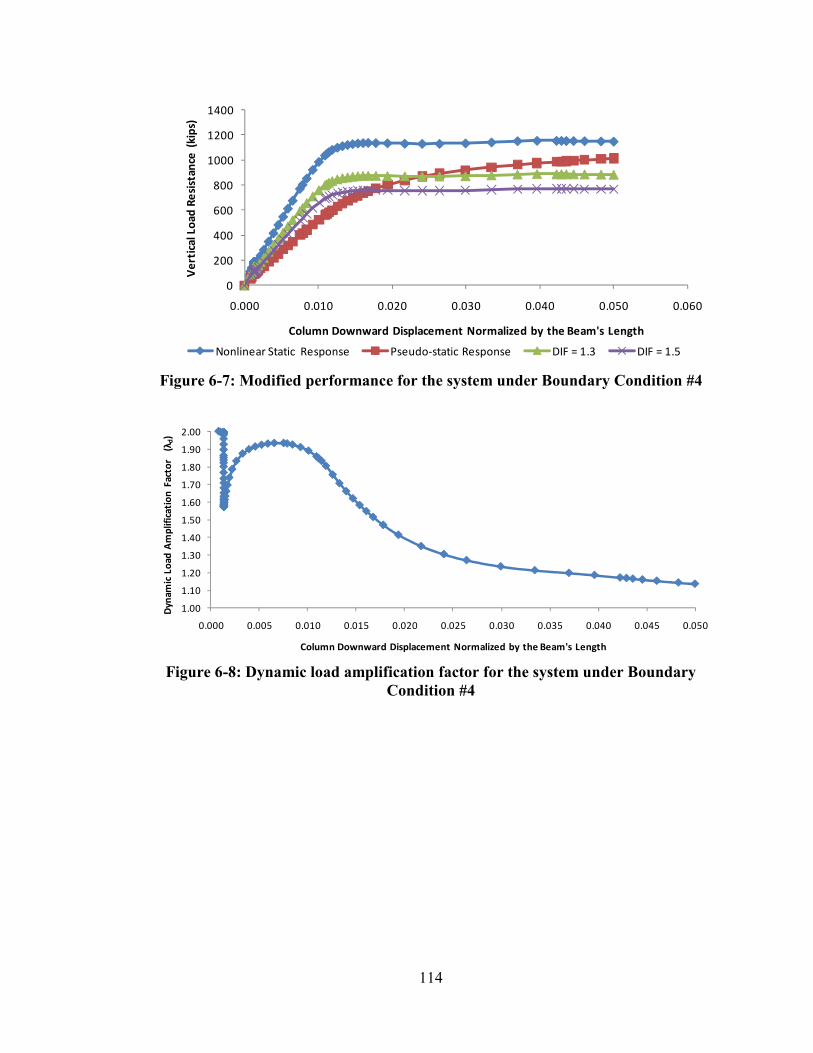
114
Figure 6-7: Modified performance for the system under Boundary Condition #4
Figure 6-8: Dynamic load amplification factor for the system under Boundary
Condition #4
0
200
400
600
800
1000
1200
1400
0.000 0.010 0.020 0.030 0.040 0.050 0.060
Ve
rtic
al L
oa
d R
esi
stan
ce (
kip
s)
Column Downward Displacement Normalized by the Beam's Length
Nonlinear Static Response Pseudo-static Response DIF = 1.3 DIF = 1.5
1.00
1.10
1.20
1.30
1.40
1.50
1.60
1.70
1.80
1.90
2.00
0.000 0.005 0.010 0.015 0.020 0.025 0.030 0.035 0.040 0.045 0.050
Dy
na
mic
Lo
ad
Am
pli
fica
tio
n F
act
or
(λ
d)
Column Downward Displacement Normalized by the Beam's Length
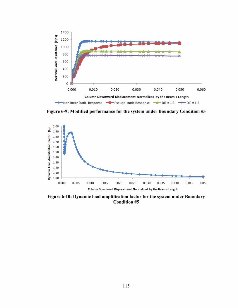
115
Figure 6-9: Modified performance for the system under Boundary Condition #5
Figure 6-10: Dynamic load amplification factor for the system under Boundary
Condition #5
0
200
400
600
800
1000
1200
1400
0.000 0.010 0.020 0.030 0.040 0.050 0.060
Ve
rtic
al L
oa
d R
esi
stan
ce (
kip
s)
Column Downward Displacement Normalized by the Beam's Length
Nonlinear Static Response Pseudo-static Response DIF = 1.3 DIF = 1.5
1.00
1.10
1.20
1.30
1.40
1.50
1.60
1.70
1.80
1.90
2.00
0.000 0.005 0.010 0.015 0.020 0.025 0.030 0.035 0.040 0.045 0.050
Dy
na
mic
Lo
ad
Am
pli
fica
tio
n F
act
or
(λ
d)
Column Downward Displacement Normalized by the Beam's Length

116
7 DEMANDS ON BOUNDARY FRAME MEMBERS
7.1 Introduction
Consideration of the demands imposed on the beams and columns by the infill panel
tension field actions (also known as: diagonal tension field action, plate tension field
action, field action, plate yielding forces, etc.) is essential to prevent the premature
boundary frame failure and hence to ensure the desirable performance of the proposed
system. The demands on the beams and columns of SPSWs under seismic load have
been investigated by Berman and Bruneau (2008) and Qu and Bruneau (2010). The
procedure developed by Berman and Bruneau (2008) to estimate the demands on the
columns consists of determination of the fundamental plastic collapse mechanism and
linear beam analysis. Their method will be used to formulate a simplified procedure for
estimating the demands on the boundary frame elements in the proposed system. Simple
FBDs for the beams and columns with infill panel tension field actions will be presented.
Based on these FBDs the demands on frame members are quantified using only linear
static analysis. For the boundary conditions illustrated in Figure 5-1, the demands on
frame members obtained from the developed simplified procedure will be compared to
those from the nonlinear static analysis using the strip model. A downward displacement
equal to 2.5% of the bay width of the frame was assumed along the damaged column in
all analysis cases. Incidentally, detailed descriptions about the strip models were
presented in Chapter 4.
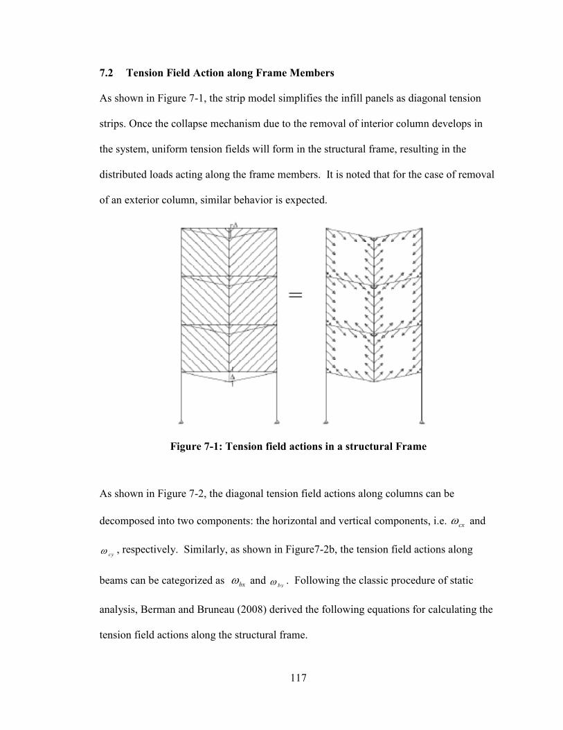
117
7.2 Tension Field Action along Frame Members
As shown in Figure 7-1, the strip model simplifies the infill panels as diagonal tension
strips. Once the collapse mechanism due to the removal of interior column develops in
the system, uniform tension fields will form in the structural frame, resulting in the
distributed loads acting along the frame members. It is noted that for the case of removal
of an exterior column, similar behavior is expected.
Figure 7-1: Tension field actions in a structural Frame
As shown in Figure 7-2, the diagonal tension field actions along columns can be
decomposed into two components: the horizontal and vertical components, i.e. cxω and
cyω , respectively. Similarly, as shown in Figure7-2b, the tension field actions along
beams can be categorized as bxω and byω . Following the classic procedure of static
analysis, Berman and Bruneau (2008) derived the following equations for calculating the
tension field actions along the structural frame.
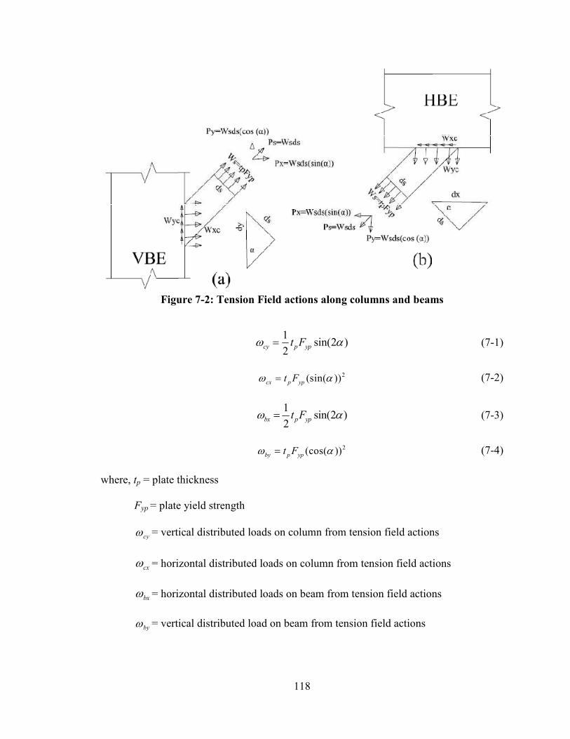
118
Figure 7-2: Tension Field actions along columns and beams
1
sin(2 )2
cy p ypt Fω α= (7-1)
2(sin( ))cx p yp
t Fω α= (7-2)
1
sin(2 )2
bx p ypt Fω α= (7-3)
2(cos( ))by p yp
t Fω α= (7-4)
where, tp = plate thickness
Fyp = plate yield strength
cyω = vertical distributed loads on column from tension field actions
cxω = horizontal distributed loads on column from tension field actions
bxω = horizontal distributed loads on beam from tension field actions
byω = vertical distributed load on beam from tension field actions
119
As suggested by equations (7-1) to (7-4) the distributed loads on each boundary frame
member depends on the thickness of the infill panel at each floor level. The required
thickness of the infill panels at different floor levels can be determine strategically based
on the vertical load resisted by the notional removed column. For simplicity, the system
presented on this thesis contains a uniform plate thickness along the different floor levels.
7.3 Demand on Beams
The demands on beams depend on the boundary conditions of the retrofitted system.
When sidesway is inhibited on both sides of the frame, the beam is subjected to: 1)
catenary action force and 2) vertical and horizontal components of the infill panel tension
field actions above and below the beam. When sidesway is uninhibited on one side or
both sides of the frame, the beam is subjected to 1) axial compression force resulted from
the horizontal component of the infill panel tension field actions acting on the columns,
and 2) vertical and horizontal components of the infill panel tension field actions above
and below the beam.

120
7.3.1 General FBDs of Beams
Figure 7-3: General FBDs of beams (a) Sidesway uninhibited (b) Sidesway inhibited
Figure 7-3 shows the FBDs for the beams under sidesway uninhibited and sidesway
inhibited boundary conditions, respectively. The simplified procedure will use these
FBDs to determine the demands on the beams. In the case when sidesway is uninhibited,
compression load, Pc, will develop at the end of the beam due to the horizontal
component of the infill panel tension field actions along the columns (Berman and
Bruneau 2008). Considering the column length tributary to each beam, the axial
compressive force on the beam becomes:
11
2 2
i icxi cxi
h hPc ω ω +
+= + (7-5)
Where, hi = story height below the beam
hi+1 = story height above the beam
cxiω and 1cxiω + = horizontal components of the tension field actions along columns
in the ith
and i+1th
story respectively.

121
Physically, the infill panel tension field actions pull the columns towards each other, and
the beams act as “shoring” to keep the columns apart. It is recognized that, when
sidesway is inhibited, the abovementioned compression force will not develop at the end
of the beams since the horizontal components of the infill panel forces will be transferred
to the horizontal restraints which prevent sidesway of the structure. In addition, due to
the presence of the horizontal restraints, the beams develop catenary action which is
denoted as Pcat in Figure 7-3b and can be calculated using equation (3-45). Note that the
catenary action only develops when sidesway is inhibited on both sides as explained in
Chapter 3. For both considered boundary conditions, i.e., the sideway uninhibited and
inhibited cases, roller supports and the axial forces determined respectively from
equations (7-5) and (3-45) are applied at the left ends of the beams, and pin supports were
assigned at the right ends. It should be noted that such boundary conditions assumed in
the FBDs are not adequate for deformation calculation however they are able to capture
the actual internal force distribution in the beams as shown in the following sections.
In addition to the axial forces acting at the ends, beams are subjected to the horizontal
and vertical components of the infill panel tension field actions above and below, i.e.,
ibxω , 1ibxω+ ,
ibyω , and
1ibyω+
as shown in Figure 7-3. While Figure 7-3 shows the general
FBDs for intermediate beams, these FBDs can also be used to determine the demands on
anchor beams (i.e. those having infill panels only on one side) by setting the infill panel
tension field actions on one side equal to zero. Moreover, when the tension field actions
above and below are identical, i.e., when the infill plates above and below an
122
intermediate beam have the same strength and thickness, the resultant infill panel forces
are equal to zero.
7.3.2 Results from Different Boundary Conditions
In order to validate the beam FBDs presented in Section 7.3.1, the demands on beams
including axial force, shear force and bending moment are compared to those obtained
from the nonlinear static push down analysis using the 2D FE model, i.e., the strip model
(see Chapter 5 for details). Described below are the detailed result comparisons for both
anchor beams and intermediate beams. Note that the demands on the beams on both
sides of the middle column are mirror images under the symmetric boundary conditions
(i.e. Boundary Conditions #1, and #3 presented in Figure 5-1). Therefore, only results
for the left-side beams were presented for such cases. In addition, since identical plates
are assumed in every floor level, the intermediate beams are expected to have the same
demands distribution. As such, only one intermediate will be studied. When plates
having different thicknesses are installed in the frame, the demands in intermediate
beams can be similarly obtained using the FBD shown in Figure 7-3.
7.3.2.1 Boundary Condition #1
Boundary condition #1 corresponds to the frame in which sidesway is uninhibited on
both sides of the frame and the interior column is removed. Under this boundary
condition, no catenary action will develop in the beams and therefore the FBD from
Figure 7-3 (a) is used.

123
7.3.2.1.1 Anchor Beams
Figure 7-4 and Figure 7-5 show the demands on the top and bottom anchor beams
respectively. It is evident that the nonlinear static analysis and the simplified procedure
give similar results. While results are only provided for the anchor beams in the left bay,
similar results can be obtained for the anchor beams in the right bay due to the symmetric
loading, geometry, and boundary conditions. As shown, the top anchor beam experiences
only compressive axial force. However, the bottom anchor beam experiences both
compressive and tensile axial forces. For the shear and bending moments, the top and
bottom anchor beams have similar distributions.

124
Figure 7-4: Axial, shear, and moment diagrams for the top anchor beam under
Boundary Condition #1
.
-700
-600
-500
-400
-300
-200
-100
0
100
200
0 50 100 150
Top
An
cho
r B
ea
m A
xia
l F
orc
e
(Kip
)
Length (in)
Nonlinear Static Analysis Simplified Procedure
-250
-200
-150
-100
-50
0
50
100
150
200
250
0 50 100 150
Top
An
cho
r B
ea
m S
he
ar
Fo
rce
(Kip
)
Length (in)
Nonlinear Static Analysis Simplified Procedure
-3000
-1000
1000
3000
5000
7000
9000
11000
0 50 100 150
Top
An
cho
r B
ea
m M
om
en
t (K
ip-i
n)
Length (in)
Nonlinear Static Analysis Simplified Procedure

125
Figure 7-5: Axial, shear, and moment diagrams for the bottom anchor beam under
Boundary Condition #1
-250
-200
-150
-100
-50
0
50
100
150
200
0 50 100 150
Bo
tto
m A
nch
or
Be
am
Ax
ial
Fo
rce
(Kip
)
Length (in)
Nonlinear Static Analysis Simplified Procedure
-250
-200
-150
-100
-50
0
50
100
150
200
0 50 100 150
Bo
tto
m A
nch
or
Be
am
Sh
ea
r
Fo
rce
(K
ip)
Length (in)
Nonlinear Static Analysis Simplified Procedure
-11000
-9000
-7000
-5000
-3000
-1000
1000
3000
0 50 100 150
Bo
tto
m A
nch
or
Be
am
Mo
me
nt
(Kip
-in
)
Length (in)
Nonlinear Static Analysis Simplified Procedure
126
7.3.2.1.2 Intermediate Beams
The axial, shear and bending moment diagrams for the intermediate beam are presented
Figure 7-6. As shown, the axial demands on the intermediate beam can be accurately
captured by the simplified procedure. Note that according to the simplified procedure the
shear and bending moment diagrams should be zero because the infill plates above and
below the intermediate beam have the same strength and thickness, resulting in identical
infill plate tension field actions and thus zero resultant forces on the intermediate beam.
The observed difference in shear and bending moment demands were caused by the
numerical errors from the nonlinear static analysis. Compared with the order of the
internal axial forces (102 kips), the observed numerical errors are negligible. It is also
recognized that the axial force at the left end of the intermediate beam is twice as much
as those at the same ends of the anchor beams because the column length tributary to the
intermediate beam is twice that of the anchor beams.
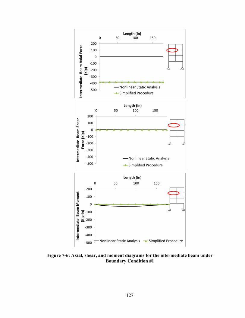
127
Figure 7-6: Axial, shear, and moment diagrams for the intermediate beam under
Boundary Condition #1
-500
-400
-300
-200
-100
0
100
200
0 50 100 150
Inte
rme
dia
te B
ea
m A
xia
l F
orc
e
(Kip
)
Length (in)
Nonlinear Static Analysis
Simplified Procedure
-500
-400
-300
-200
-100
0
100
200
0 50 100 150
Inte
rme
dia
te B
ea
m S
he
ar
Fo
rce
(K
ip)
Length (in)
Nonlinear Static Analysis
Simplified Procedure
-500
-400
-300
-200
-100
0
100
200
0 50 100 150
Inte
rme
dia
te B
ea
m M
om
en
t
(Kip
-in
)
Length (in)
Nonlinear Static Analysis Simplified Procedure

128
7.3.2.2 Boundary Condition #2
Under Boundary Condition #2, the interior column is removed and sidesway is only
inhibited on the left side of the frame. As a result, the catenary action will not develop in
the beams due to the absence of the anchorage on the right side of the frame. Therefore,
the FBD presented in Figure 7-3(a) is used in the simplified procedure. It is expected that
the beam demands under Boundary Condition 2 will be identical to the corresponding
results under Boundary Condition #1. This point is further confirmed by the results
presented in Sections 7.3.2.2.1 and 7.3.2.2.2.
7.3.2.2.1 Anchor Beams
Figure 7-7 and Figure 7-8, illustrate the axial, shear and bending moment diagrams for
the top and bottom anchor beams. As shown, the results predicted from the proposed
FBDs agree well with those obtained from the nonlinear static analysis. In addition, the
demand distributions along the anchor beams under Boundary Condition #2 is the same
as those under Boundary condition #1 (see Figure 7-4 ,Figure 7-5, Figure 7-7 and Figure
7-8).
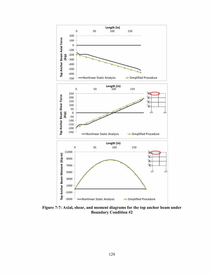
129
Figure 7-7: Axial, shear, and moment diagrams for the top anchor beam under
Boundary Condition #2
-700
-600
-500
-400
-300
-200
-100
0
100
200
0 50 100 150
Top
An
cho
r B
ea
m A
xia
l F
orc
e
(Kip
)
Length (in)
Nonlinear Static Analysis Simplified Procedure
-250
-200
-150
-100
-50
0
50
100
150
200
250
0 50 100 150
Top
An
cho
r B
ea
m S
he
ar
Fo
rce
(Kip
)
Length (in)
Nonlinear Static Analysis Simplified Procedure
-3000
-1000
1000
3000
5000
7000
9000
11000
0 50 100 150
Top
An
cho
r B
ea
m M
om
en
t (K
ip-i
n)
Length (in)
Nonlinear Static Analysis Simplified Procedure
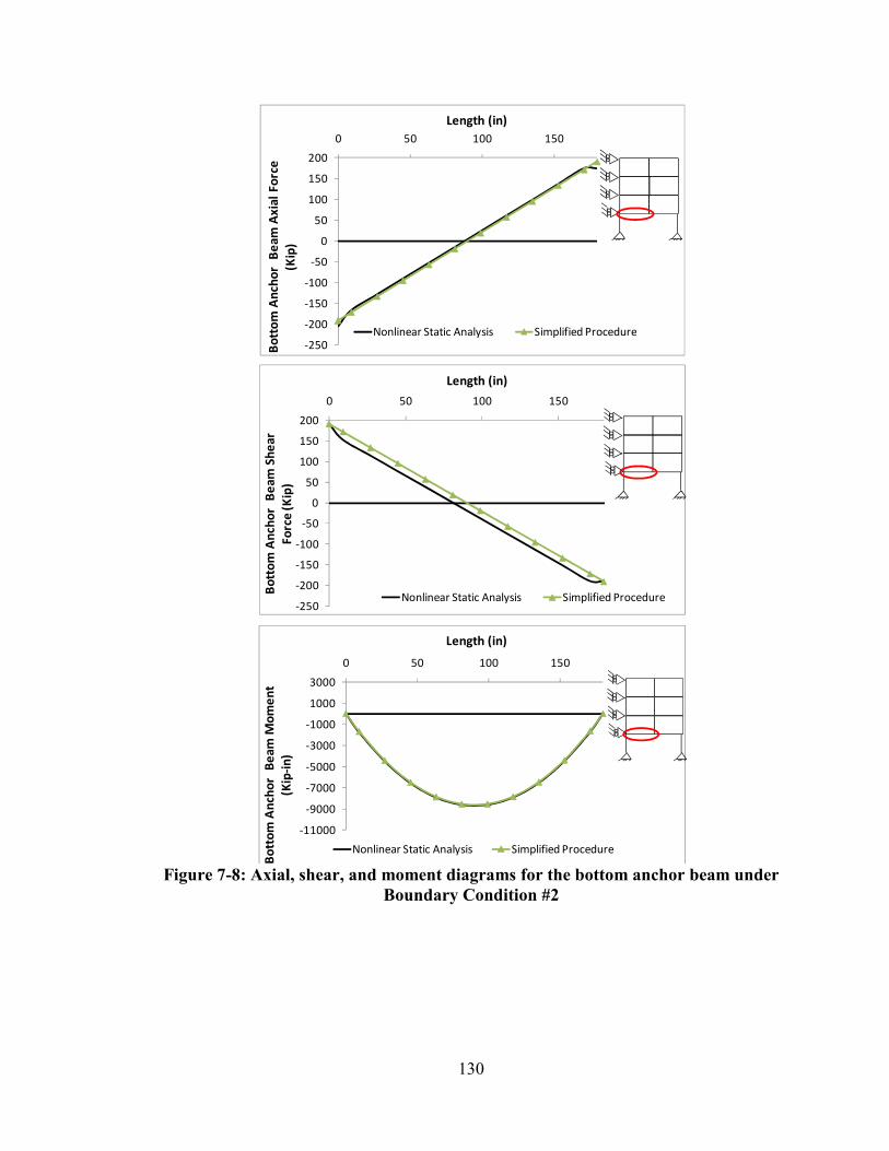
130
Figure 7-8: Axial, shear, and moment diagrams for the bottom anchor beam under
Boundary Condition #2
-250
-200
-150
-100
-50
0
50
100
150
200
0 50 100 150
Bo
tto
m A
nch
or
Be
am
Ax
ial
Fo
rce
(Kip
)
Length (in)
Nonlinear Static Analysis Simplified Procedure
-250
-200
-150
-100
-50
0
50
100
150
200
0 50 100 150
Bo
tto
m A
nch
or
Be
am
Sh
ea
r
Fo
rce
(K
ip)
Length (in)
Nonlinear Static Analysis Simplified Procedure
-11000
-9000
-7000
-5000
-3000
-1000
1000
3000
0 50 100 150
Bo
tto
m A
nch
or
Be
am
Mo
me
nt
(Kip
-in
)
Length (in)
Nonlinear Static Analysis Simplified Procedure

131
7.3.2.2.2 Intermediate Beams
The axial, shear, and bending moment diagrams for the intermediate beams are presented
in Figure 7-9. As shown, similar to the anchor beams, the demand distributions in the
intermediate beams under Boundary Condition #2 is the same as those under Boundary
Condition #1 (see Figure 7-6).
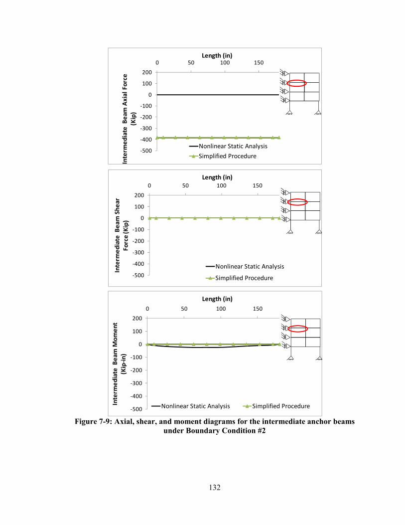
132
Figure 7-9: Axial, shear, and moment diagrams for the intermediate anchor beams
under Boundary Condition #2
-500
-400
-300
-200
-100
0
100
200
0 50 100 150
Inte
rme
dia
te B
ea
m A
xia
l F
orc
e
(Kip
)
Length (in)
Nonlinear Static Analysis
Simplified Procedure
-500
-400
-300
-200
-100
0
100
200
0 50 100 150
Inte
rme
dia
te B
ea
m S
he
ar
Fo
rce
(K
ip)
Length (in)
Nonlinear Static Analysis
Simplified Procedure
-500
-400
-300
-200
-100
0
100
200
0 50 100 150
Inte
rme
dia
te B
ea
m M
om
en
t
(Kip
-in
)
Length (in)
Nonlinear Static Analysis Simplified Procedure

133
7.3.2.3 Boundary Condition #3
Boundary Condition # 3 considers the removal of interior column and assigns the lateral
displacement restraints (i.e. sideway inhibited) on both sides of the frame. Due to the
presence of restraints, all beams are expected to develop catenary action. Therefore, the
FBD presented in Figure 7-3(b) is used to calculate the beam demands.
7.3.2.3.1 Anchor Beams
The axial, shear, and bending moment diagrams for the top and bottom anchor beams
under Boundary Condition#3 are shown in Figure 7-10 and Figure 7-11, respectively.
Compared to the anchor beams under Boundary Conditions #1 and #2, the axial tension
forces in the anchor beams under Boundary Condition #3 are significantly larger due to
the development of catenary action.

134
Figure 7-10: Axial, shear, and moment diagrams for the top anchor beam under
Boundary Condition #3
-300
-100
100
300
500
700
900
1100
0 20 40 60 80 100 120 140 160 180
Top
An
cho
r B
ea
m A
xia
l
Fo
rce
(K
ip)
Length (in)
Nonlinear Static Analysis Simplified Procedure
-300
-200
-100
0
100
200
300
0 20 40 60 80 100 120 140 160 180
Top
An
cho
r B
ea
m S
he
ar
Fo
rce
(K
ip)
Length (in)
Nonlinear Static Analysis Simplified Procedure
-3000
-1000
1000
3000
5000
7000
9000
11000
0 20 40 60 80 100 120 140 160 180
Top
An
cho
r B
ea
m M
om
en
t
(kip
-in
)
Length (in)
Nonlinear Static Analysis Simplified Procedure
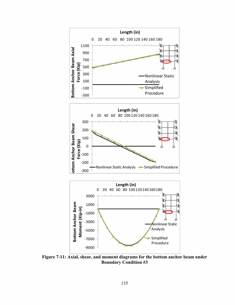
135
Figure 7-11: Axial, shear, and moment diagrams for the bottom anchor beam under
Boundary Condition #3
-300
-200
-100
0
100
200
300
0 20 40 60 80 100 120 140 160 180
Bo
tto
m A
nch
or
Be
am
Sh
ea
r
Fo
rce
(K
ip)
Length (in)
Nonlinear Static Analysis Simplified Procedure
-300
-100
100
300
500
700
900
1100
0 20 40 60 80 100 120 140 160 180
Bo
tto
m A
nch
or
Be
am
Ax
ial
Fo
rce
(K
ip)
Length (in)
Nonlinear Static
Analysis
Simplified
Procedure
-9000
-7000
-5000
-3000
-1000
1000
3000
0 20 40 60 80 100 120140 160 180
Bo
tto
m A
nch
or
Be
am
Mo
me
nt
(Kip
-in
)
Length (in)
Nonlinear Static
Analysis
Simplified
Procedure
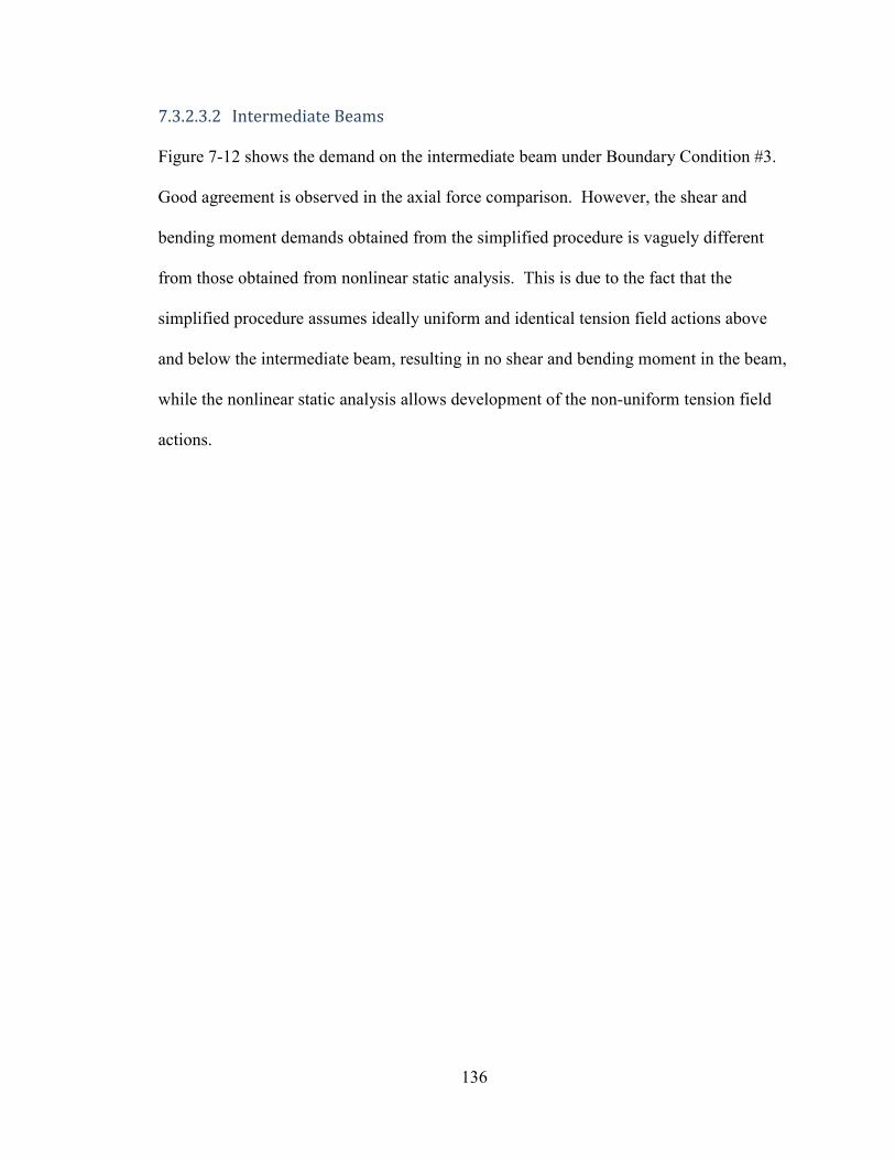
136
7.3.2.3.2 Intermediate Beams
Figure 7-12 shows the demand on the intermediate beam under Boundary Condition #3.
Good agreement is observed in the axial force comparison. However, the shear and
bending moment demands obtained from the simplified procedure is vaguely different
from those obtained from nonlinear static analysis. This is due to the fact that the
simplified procedure assumes ideally uniform and identical tension field actions above
and below the intermediate beam, resulting in no shear and bending moment in the beam,
while the nonlinear static analysis allows development of the non-uniform tension field
actions.

137
Figure 7-12: Axial, shear, and moment diagrams for the intermediate beams under
Boundary Condition #3
-200
0
200
400
600
800
0 20 40 60 80 100 120 140 160 180
Inte
rme
dia
te B
ea
m A
xia
l
Fo
rce
(K
ip)
Length (in)
Nonlinear Static Analysis Simplified Procedure
-200
0
200
400
600
800
0 20 40 60 80 100 120 140 160 180
Inte
rme
dia
te B
ea
m S
he
ar
Fo
rce
(K
ip)
Length (in)
Nonlinear Static Analysis Simplified Procedure
-200
0
200
400
600
800
0 20 40 60 80 100 120 140 160 180
Inte
rme
dia
te B
ea
m
Mo
me
nt
(Kip
-in
)
Length (in)
Nonlinear Static Analysis Simplified Procedure

138
7.3.2.4 Boundary Condition #4
Boundary Condition #4 accounts for removal of the exterior column at the bottom story
and allows lateral deformation at the left side of the frame. For this boundary condition
beam catenary action does not develop. As such, the FBD presented in Figure 7-3(a) is
used to determine the demand on the beams.
7.3.2.4.1 Anchor Beams
For Boundary Condition #4, geometric symmetry no longer applies and the two top
anchors and the two bottom anchors beams (on each side of the interior column) were
consider respectively.
The axial, shear, and bending moments for the top right and bottom right anchor beams
are respectively shown in Figure 7-13 and Figure 7-14 and good agreements are observed
between the results from the simplified procedure and the nonlinear static analysis.
The demands for the top left and bottom left anchor beams are shown in Figure 7-15 and
Figure 7-16, respectively. Good agreements are observed in all comparisons except that
the axial force in the top left anchor beam predicted by the simplified procedure is
slightly different from that from nonlinear static analysis. This observation can be
attributed to the fact that the FBD considered in the simplified procedure assumes
uniform yielding of the infill plate that is unlikely to develop under this boundary
condition. However, the observed difference is acceptable from the design perspective.
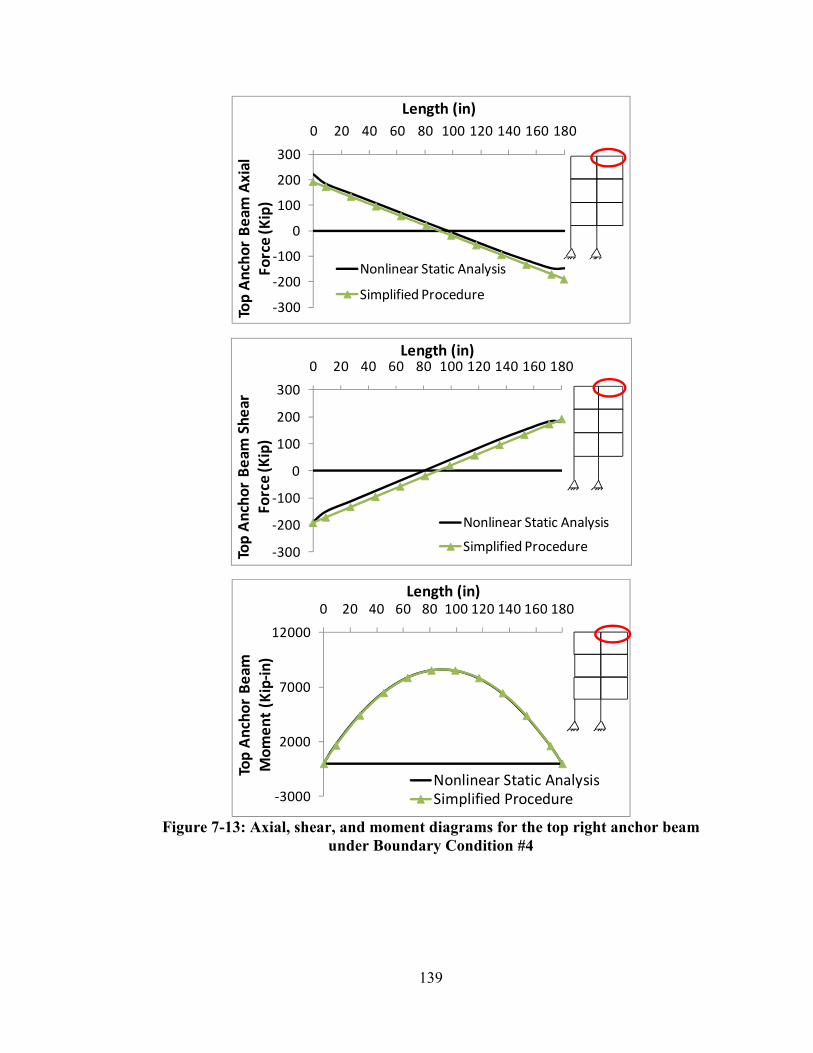
139
Figure 7-13: Axial, shear, and moment diagrams for the top right anchor beam
under Boundary Condition #4
-300
-200
-100
0
100
200
300
0 20 40 60 80 100 120 140 160 180
Top
An
cho
r B
ea
m A
xia
l
Fo
rce
(K
ip)
Length (in)
Nonlinear Static Analysis
Simplified Procedure
-300
-200
-100
0
100
200
300
0 20 40 60 80 100 120 140 160 180
Top
An
cho
r B
ea
m S
he
ar
Fo
rce
(K
ip)
Length (in)
Nonlinear Static Analysis
Simplified Procedure
-3000
2000
7000
12000
0 20 40 60 80 100 120 140 160 180
Top
An
cho
r B
ea
m
Mo
me
nt
(Kip
-in
)
Length (in)
Nonlinear Static Analysis
Simplified Procedure
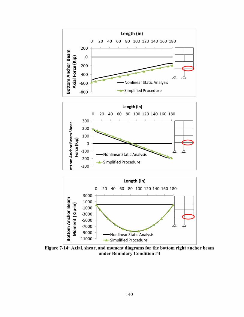
140
Figure 7-14: Axial, shear, and moment diagrams for the bottom right anchor beam
under Boundary Condition #4
-800
-600
-400
-200
0
200
0 20 40 60 80 100 120 140 160 180
Bo
tto
m A
nch
or
Be
am
Ax
ial
Fo
rce
(K
ip)
Length (in)
Nonlinear Static Analysis
Simplified Procedure
-300
-200
-100
0
100
200
300
0 20 40 60 80 100 120 140 160 180
Bo
tto
m A
nch
or
Be
am
Sh
ea
r
Fo
rce
(K
ip)
Length (in)
Nonlinear Static Analysis
Simplified Procedure
-11000
-9000
-7000
-5000
-3000
-1000
1000
3000
0 20 40 60 80 100 120 140 160 180
Bo
tto
m A
nch
or
Be
am
Mo
me
nt
(Kip
-in
)
Length (in)
Nonlinear Static Analysis
Simplified Procedure
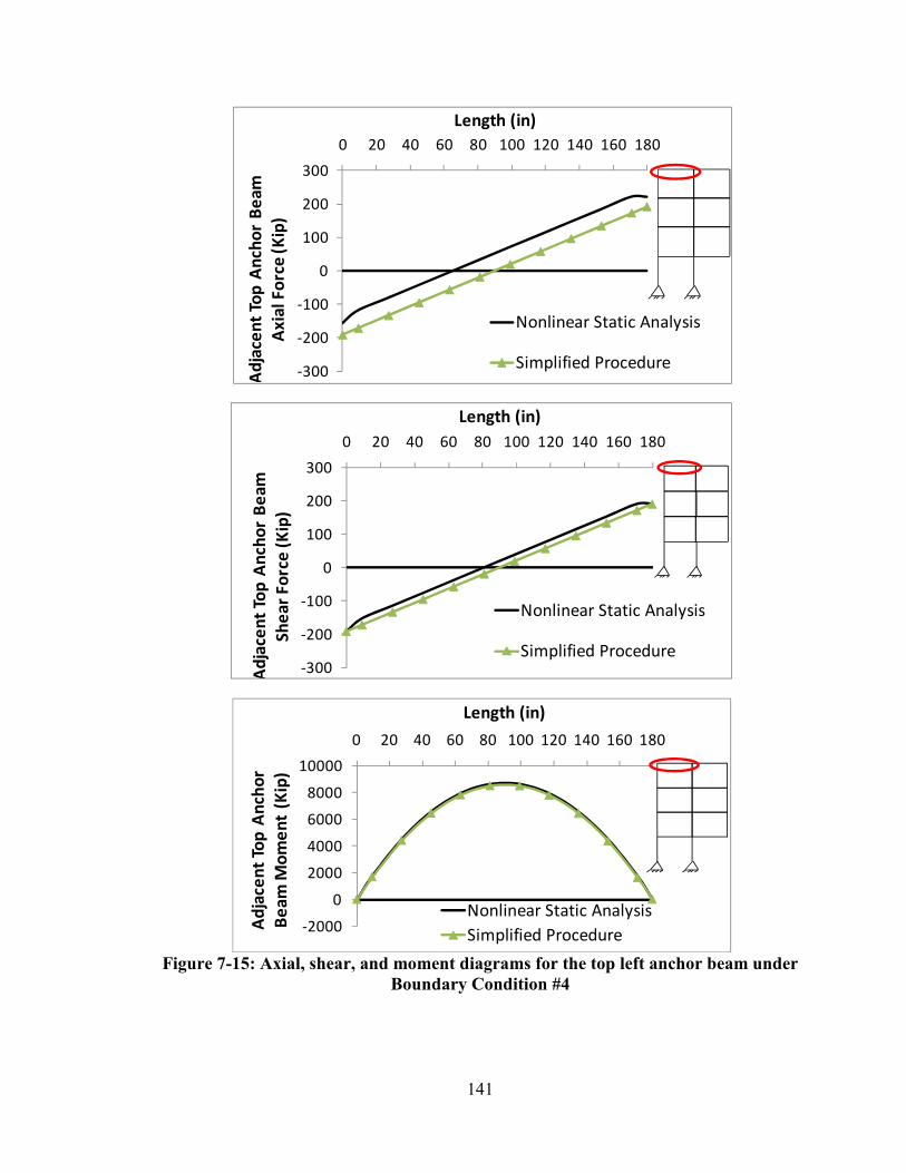
141
Figure 7-15: Axial, shear, and moment diagrams for the top left anchor beam under
Boundary Condition #4
-300
-200
-100
0
100
200
300
0 20 40 60 80 100 120 140 160 180
Ad
jace
nt
Top
An
cho
r B
ea
m
Ax
ial
Fo
rce
(K
ip)
Length (in)
Nonlinear Static Analysis
Simplified Procedure
-300
-200
-100
0
100
200
300
0 20 40 60 80 100 120 140 160 180
Ad
jace
nt
Top
An
cho
r B
ea
m
Sh
ea
r F
orc
e (
Kip
)
Length (in)
Nonlinear Static Analysis
Simplified Procedure
-2000
0
2000
4000
6000
8000
10000
0 20 40 60 80 100 120 140 160 180
Ad
jace
nt
Top
An
cho
r
Be
am
Mo
me
nt
(Kip
)
Length (in)
Nonlinear Static Analysis
Simplified Procedure
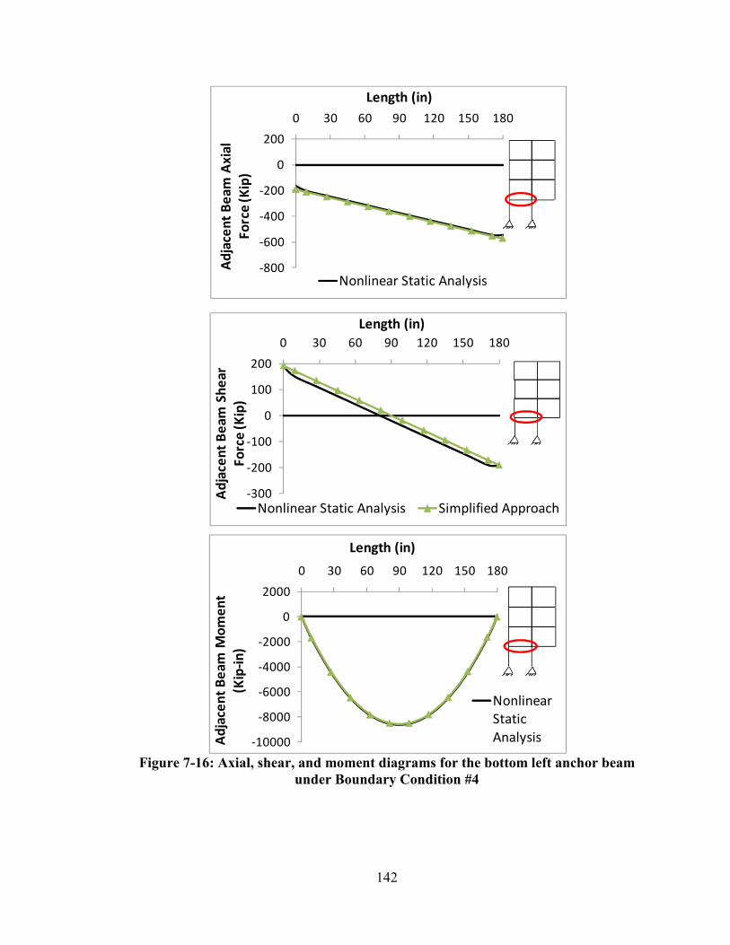
142
Figure 7-16: Axial, shear, and moment diagrams for the bottom left anchor beam
under Boundary Condition #4
-800
-600
-400
-200
0
200
0 30 60 90 120 150 180
Ad
jace
nt
Be
am
Ax
ial
Fo
rce
(K
ip)
Length (in)
Nonlinear Static Analysis
-300
-200
-100
0
100
200
0 30 60 90 120 150 180
Ad
jace
nt
Be
am
Sh
ea
r
Fo
rce
(K
ip)
Length (in)
Nonlinear Static Analysis Simplified Approach
-10000
-8000
-6000
-4000
-2000
0
2000
0 30 60 90 120 150 180
Ad
jace
nt
Be
am
Mo
me
nt
(Kip
-in
)
Length (in)
Nonlinear
Static
Analysis
143
7.3.2.4.2 Intermediate Beams
Under Boundary Condition #4, the four intermediate beams are expected to have
identical or symmetric demand distribution. As such, only one intermediate beam was
selected for analysis. The axial demand in the intermediate beam can be satisfactorily
approximated by the simplified procedure as shown in Figure 7-17. However, slight
differences are observed in the shear and moment comparisons due to numerical errors in
the nonlinear static analysis model.

144
Figure 7-17: Axial, shear, and moment diagrams for the intermediate beams under
Boundary Condition #4
-500
-400
-300
-200
-100
0
100
200
0 20 40 60 80 100 120 140 160 180
Inte
rme
dia
te B
ea
m A
xia
l
Fo
rce
(K
ip)
Length (in)
Nonlinear Static Analysis
Simplified Procedure
-500
-400
-300
-200
-100
0
100
200
0 20 40 60 80 100 120 140 160 180
Inte
rme
dia
te B
ea
m
Sh
ea
rs F
orc
e (
Kip
)
Length (in)
Nonlinear Static Analysis
Simplified Procedure
-500
-400
-300
-200
-100
0
100
200
0 20 40 60 80 100 120 140 160 180
Inte
rme
dia
te B
ea
m
Mo
me
nt
(Kip
-in
)
Length (in)
Nonlinear Static Analysis
Simplified Procedure

145
7.3.2.5 Boundary Condition #5
Boundary Condition #5 takes into account the loss of the exterior column at the bottom
story and inhibits the sideway deformation on the left side of the frame. Under such a
boundary condition, the catenary action does not develop in the beams due to the absence
of anchorage effects on the right side of the frame. Thus, the FBD presented in Figure
7-3(a) is used to quantify the demands in the beams.
7.3.2.5.1 Anchor Beam
The axial, shear, and bending moment diagrams for the right top and bottom anchor
beams under Boundary Condition#5, are presented in Figure 7-18 and Figure 7-19,
respectively. Note that the demands on these anchor beams are identical to those under
Boundary Condition #4 (see Figure 7-13 and Figure 7-14 for details).
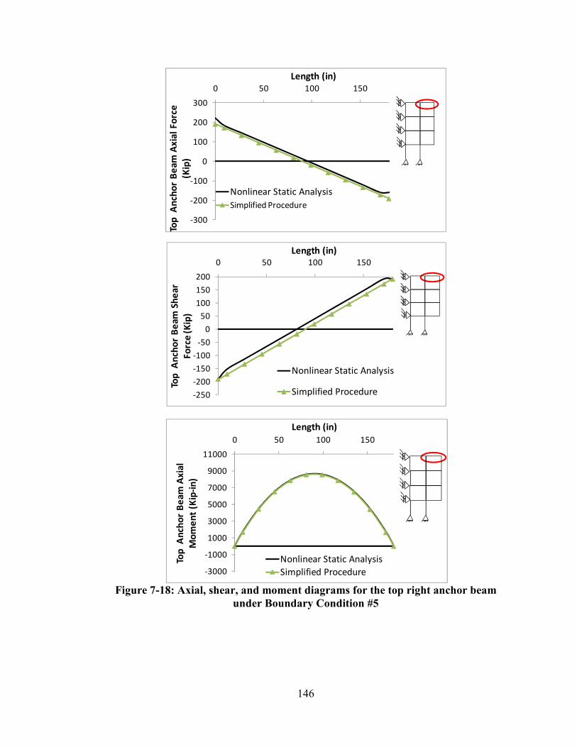
146
Figure 7-18: Axial, shear, and moment diagrams for the top right anchor beam
under Boundary Condition #5
-300
-200
-100
0
100
200
300
0 50 100 150
Top
A
nch
or
Be
am
Ax
ial
Fo
rce
(Kip
)
Length (in)
Nonlinear Static Analysis
Simplified Procedure
-250
-200
-150
-100
-50
0
50
100
150
200
0 50 100 150
Top
A
nch
or
Be
am
Sh
ea
r
Fo
rce
(K
ip)
Length (in)
Nonlinear Static Analysis
Simplified Procedure
-3000
-1000
1000
3000
5000
7000
9000
11000
0 50 100 150
Top
A
nch
or
Be
am
Ax
ial
Mo
me
nt
(Kip
-in
)
Length (in)
Nonlinear Static Analysis
Simplified Procedure

147
Figure 7-19: Axial, shear, and moment diagrams for the bottom right anchor beam
under Boundary Condition #5
-700
-600
-500
-400
-300
-200
-100
0
100
200
0 50 100 150
Bo
tto
m A
nch
or
Be
am
Ax
ial
Fo
rce
(K
ip)
Length (in)
Nonlinear Static Analysis
Simplified Procedure
-250
-200
-150
-100
-50
0
50
100
150
200
250
0 50 100 150
Bo
tto
m A
nch
or
HB
E B
ea
m F
orc
e
(Kip
)
Length (in)
Nonlinear Static
AnalysisSimplified
Procedure
-10000
-8000
-6000
-4000
-2000
0
2000
0 50 100 150
Bo
tto
m A
nch
or
Be
am
Mo
me
nt
(Kip
-in
)
Length (in)
Nonlinear Static
Analysis
Simplified
Procedure

148
The demands on the left anchor beams under Boundary Condition#5 cannot be estimated
using the FBDs because the infill panels installed in the left bay of the frame do not form
the diagonal tension field actions that are assumed in the FBDs. As such, only the results
from the nonlinear static analysis are provided in Figure 7-20 and Figure 7-21.
Compared to the corresponding results from the other boundary conditions, the top and
bottom anchor beams on the left side of the frame have relatively low demands due to the
incomplete development of the tension field actions.
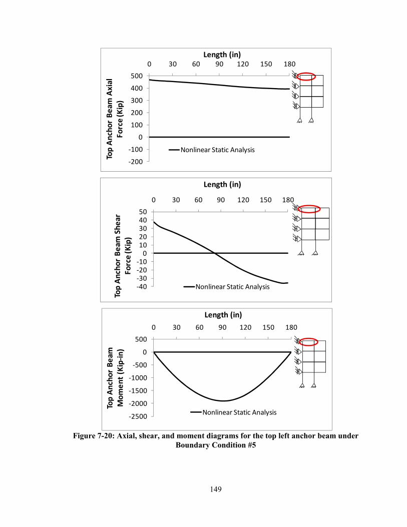
149
Figure 7-20: Axial, shear, and moment diagrams for the top left anchor beam under
Boundary Condition #5
-200
-100
0
100
200
300
400
500
0 30 60 90 120 150 180
Top
An
cho
r B
ea
m A
xia
l
Fo
rce
(K
ip)
Length (in)
Nonlinear Static Analysis
-40
-30
-20
-10
0
10
20
30
40
50
0 30 60 90 120 150 180
Top
An
ch
or
Be
am
Sh
ea
r
Fo
rce
(K
ip)
Length (in)
Nonlinear Static Analysis
-2500
-2000
-1500
-1000
-500
0
500
0 30 60 90 120 150 180
Top
An
cho
r B
ea
m
Mo
me
nt
(Kip
-in
)
Length (in)
Nonlinear Static Analysis

150
Figure 7-21: Axial, shear, and moment diagrams for the bottom left anchor beam
under Boundary Condition #5
-400
-300
-200
-100
0
100
200
0 30 60 90 120 150 180
Bo
tto
m A
nch
or
Be
am
Ax
ial
Fo
rce
(K
ip)
Length (in)
Nonlinear Static Analysis
-30
-25
-20
-15
-10
-5
0
5
10
15
0 30 60 90 120 150 180
Bo
tto
m A
nch
or
Be
am
Sh
ea
r
Fo
rce
(K
ip)
Length (in)
Nonlinear Static Analysis
-300
-100
100
300
500
700
900
1100
0 30 60 90 120 150 180
Bo
tto
m A
nch
or
Be
am
Mo
me
nt
(Kip
-in
)
Length (in)
Nonlinear Static Analysis
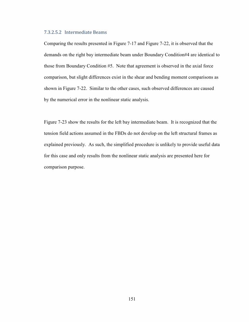
151
7.3.2.5.2 Intermediate Beams
Comparing the results presented in Figure 7-17 and Figure 7-22, it is observed that the
demands on the right bay intermediate beam under Boundary Condition#4 are identical to
those from Boundary Condition #5. Note that agreement is observed in the axial force
comparison, but slight differences exist in the shear and bending moment comparisons as
shown in Figure 7-22. Similar to the other cases, such observed differences are caused
by the numerical error in the nonlinear static analysis.
Figure 7-23 show the results for the left bay intermediate beam. It is recognized that the
tension field actions assumed in the FBDs do not develop on the left structural frames as
explained previously. As such, the simplified procedure is unlikely to provide useful data
for this case and only results from the nonlinear static analysis are presented here for
comparison purpose.

152
Figure 7-22: Axial, shear, and moment diagrams for the right intermediate beams
under Boundary Condition #5
-500
-400
-300
-200
-100
0
100
200
0 50 100 150
Inte
rme
dia
te B
ea
m A
xia
l
Fo
rce
(K
ip)
Length (in)
Nonlinear Static Analysis Simplified Procedure
-500
-400
-300
-200
-100
0
100
200
0 50 100 150
Inte
rme
dia
te B
ea
m S
he
ar
Fo
rce
(K
ip)
Length (in)
Nonlinear Static
Analysis
Simplified Procedure
-500
-400
-300
-200
-100
0
100
200
0 50 100 150
Inte
rme
dia
te B
ea
m M
om
en
t
(Kip
-in
)
Length (in)
Nonlinear Static
Procedure
Simplified
Procedure
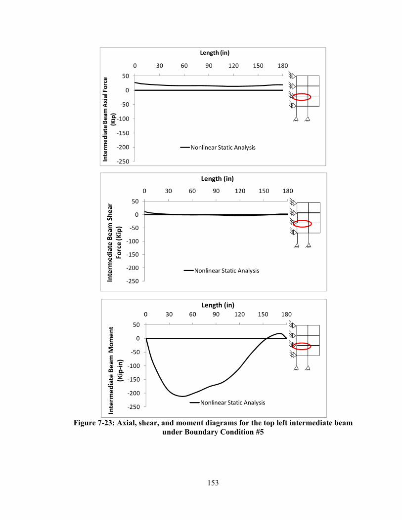
153
Figure 7-23: Axial, shear, and moment diagrams for the top left intermediate beam
under Boundary Condition #5
-250
-200
-150
-100
-50
0
50
0 30 60 90 120 150 180
Inte
rme
dia
te B
ea
m A
xia
l Fo
rce
(Kip
)
Length (in)
Nonlinear Static Analysis
-250
-200
-150
-100
-50
0
50
0 30 60 90 120 150 180
Inte
rme
dia
te B
ea
m S
he
ar
Fo
rce
(K
ip)
Length (in)
Nonlinear Static Analysis
-250
-200
-150
-100
-50
0
50
0 30 60 90 120 150 180
Inte
rme
dia
te B
ea
m M
om
en
t
(Kip
-in
)
Length (in)
Nonlinear Static Analysis
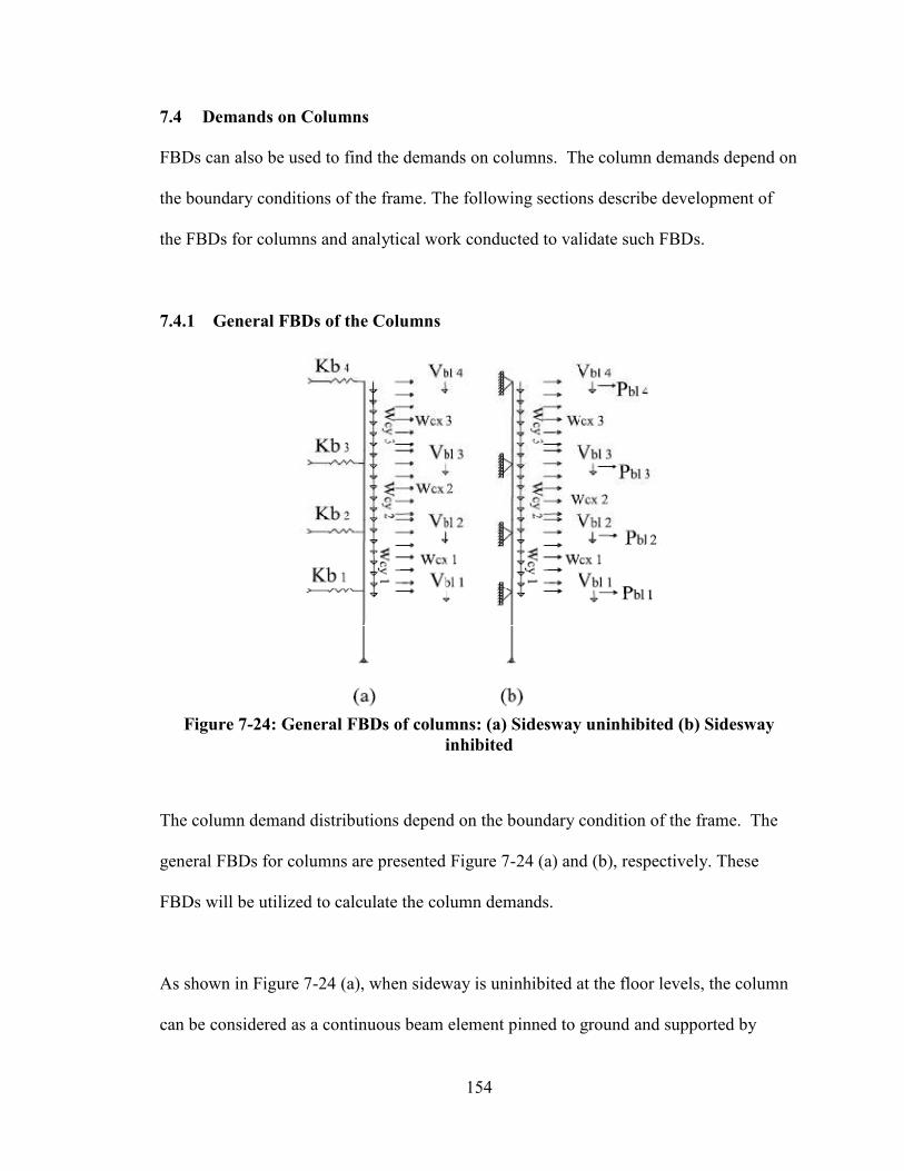
154
7.4 Demands on Columns
FBDs can also be used to find the demands on columns. The column demands depend on
the boundary conditions of the frame. The following sections describe development of
the FBDs for columns and analytical work conducted to validate such FBDs.
7.4.1 General FBDs of the Columns
Figure 7-24: General FBDs of columns: (a) Sidesway uninhibited (b) Sidesway
inhibited
The column demand distributions depend on the boundary condition of the frame. The
general FBDs for columns are presented Figure 7-24 (a) and (b), respectively. These
FBDs will be utilized to calculate the column demands.
As shown in Figure 7-24 (a), when sideway is uninhibited at the floor levels, the column
can be considered as a continuous beam element pinned to ground and supported by
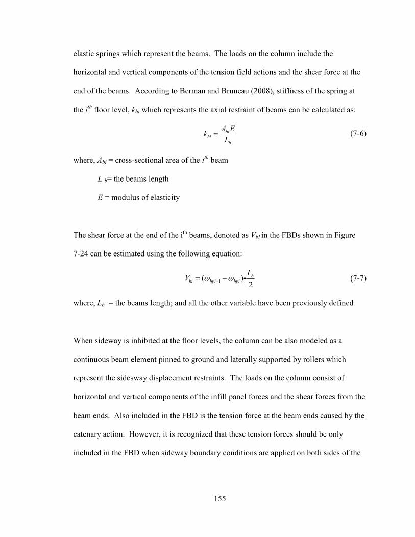
155
elastic springs which represent the beams. The loads on the column include the
horizontal and vertical components of the tension field actions and the shear force at the
end of the beams. According to Berman and Bruneau (2008), stiffness of the spring at
the ith
floor level, kbi which represents the axial restraint of beams can be calculated as:
bibi
b
A Ek
L= (7-6)
where, Abi = cross-sectional area of the ith
beam
L b= the beams length
E = modulus of elasticity
The shear force at the end of the ith
beams, denoted as Vbi in the FBDs shown in Figure
7-24 can be estimated using the following equation:
1( )2
bbi byi byi
LV ω ω+= − i (7-7)
where, Lb = the beams length; and all the other variable have been previously defined
When sideway is inhibited at the floor levels, the column can be also modeled as a
continuous beam element pinned to ground and laterally supported by rollers which
represent the sidesway displacement restraints. The loads on the column consist of
horizontal and vertical components of the infill panel forces and the shear forces from the
beam ends. Also included in the FBD is the tension force at the beam ends caused by the
catenary action. However, it is recognized that these tension forces should be only
included in the FBD when sideway boundary conditions are applied on both sides of the
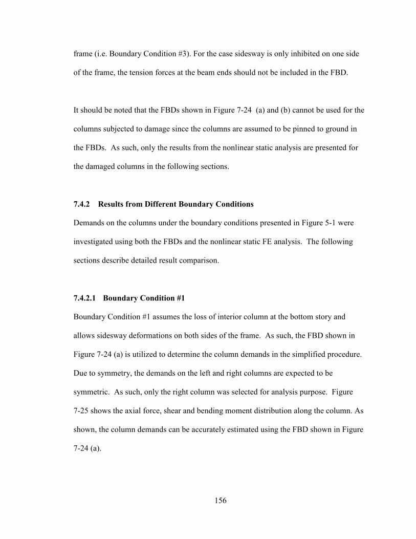
156
frame (i.e. Boundary Condition #3). For the case sidesway is only inhibited on one side
of the frame, the tension forces at the beam ends should not be included in the FBD.
It should be noted that the FBDs shown in Figure 7-24 (a) and (b) cannot be used for the
columns subjected to damage since the columns are assumed to be pinned to ground in
the FBDs. As such, only the results from the nonlinear static analysis are presented for
the damaged columns in the following sections.
7.4.2 Results from Different Boundary Conditions
Demands on the columns under the boundary conditions presented in Figure 5-1 were
investigated using both the FBDs and the nonlinear static FE analysis. The following
sections describe detailed result comparison.
7.4.2.1 Boundary Condition #1
Boundary Condition #1 assumes the loss of interior column at the bottom story and
allows sidesway deformations on both sides of the frame. As such, the FBD shown in
Figure 7-24 (a) is utilized to determine the column demands in the simplified procedure.
Due to symmetry, the demands on the left and right columns are expected to be
symmetric. As such, only the right column was selected for analysis purpose. Figure
7-25 shows the axial force, shear and bending moment distribution along the column. As
shown, the column demands can be accurately estimated using the FBD shown in Figure
7-24 (a).
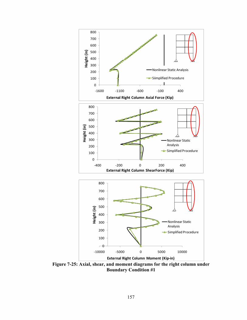
157
Figure 7-25: Axial, shear, and moment diagrams for the right column under
Boundary Condition #1
0
100
200
300
400
500
600
700
800
-400 -200 0 200 400
He
igh
t (i
n)
External Right Column ShearForce (Kip)
Nonlinear Static
Analysis
Simplified Procedure
0
100
200
300
400
500
600
700
800
-1600 -1100 -600 -100 400
He
igh
t (i
n)
External Right Column Axial Force (Kip)
Nonlinear Static Analysis
Siimplified Procedure
0
100
200
300
400
500
600
700
800
-10000 -5000 0 5000 10000
He
igh
t (i
n)
External Right Column Moment (Kip-in)
Nonlinear Static
Analysis
Simplified Procedure

158
In addition to the exterior columns, the interior column which suffered from damages at
the bottom story was also investigated. Given that the FBDs shown in Figure 7-24
assumes that the columns are pinned to the ground, the simplified procedure is not able to
predict the column demands. As such, only results from the nonlinear static analysis are
presented in Figure 7-26. It is noteworthy that the shear and bending moment in the
interior column are zero since the loads (including tension field actions and forces at the
beam ends) on both sides of the column are mirror images.
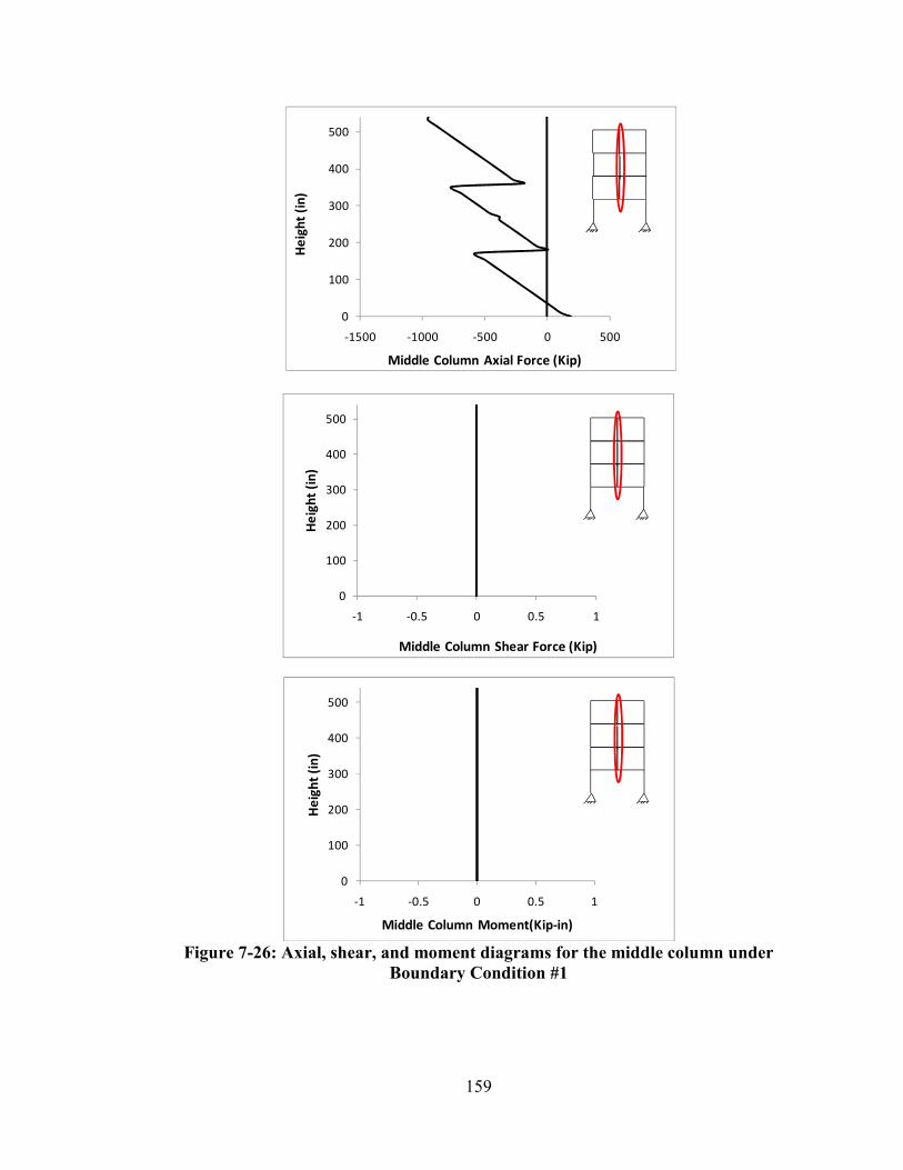
159
Figure 7-26: Axial, shear, and moment diagrams for the middle column under
Boundary Condition #1
0
100
200
300
400
500
-1500 -1000 -500 0 500
He
igh
t (i
n)
Middle Column Axial Force (Kip)
0
100
200
300
400
500
-1 -0.5 0 0.5 1
He
igh
t (i
n)
Middle Column Shear Force (Kip)
0
100
200
300
400
500
-1 -0.5 0 0.5 1
He
igh
t (i
n)
Middle Column Moment(Kip-in)

160
7.4.2.2 Boundary Condition #2
Boundary Condition #2 accounts for the loss of interior column at the bottom story and
assigns sideway inhibited restraints only on the left side of the frame (note: lateral
deformation is allowed at the right side of the frame). Due to the absence of the
anchorage on the right side of the frame, catenary action does not develop in the beams.
Therefore, the FBDs shown in Figure 7-24(a) and (b) were utilized to calculate the
demands on the exterior columns on the right and left sides of the frame, respectively.
Figure 7-27 and Figure 7-28 illustrate the axial, shear and bending moment diagram for
the right and left exterior columns, respectively. As show, the demand distributions are
either identical or symmetric in both columns. Figure 7-29 shows the demands on the
interior column which is damaged at the first story. For the reason presented previously,
only results from the nonlinear static analysis are presented.
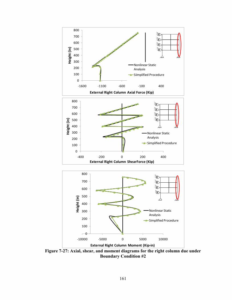
161
Figure 7-27: Axial, shear, and moment diagrams for the right column due under
Boundary Condition #2
0
100
200
300
400
500
600
700
800
-1600 -1100 -600 -100 400
He
igh
t (i
n)
External Right Column Axial Force (Kip)
Nonlinear Static
Analysis
Siimplified Procedure
0
100
200
300
400
500
600
700
800
-400 -200 0 200 400
He
igh
t (i
n)
External Right Column ShearForce (Kip)
Nonlinear Static
Analysis
Simplified Procedure
0
100
200
300
400
500
600
700
800
-10000 -5000 0 5000 10000
He
igh
t (i
n)
External Right Column Moment (Kip-in)
Nonlinear Static
Analysis
Simplified Procedure
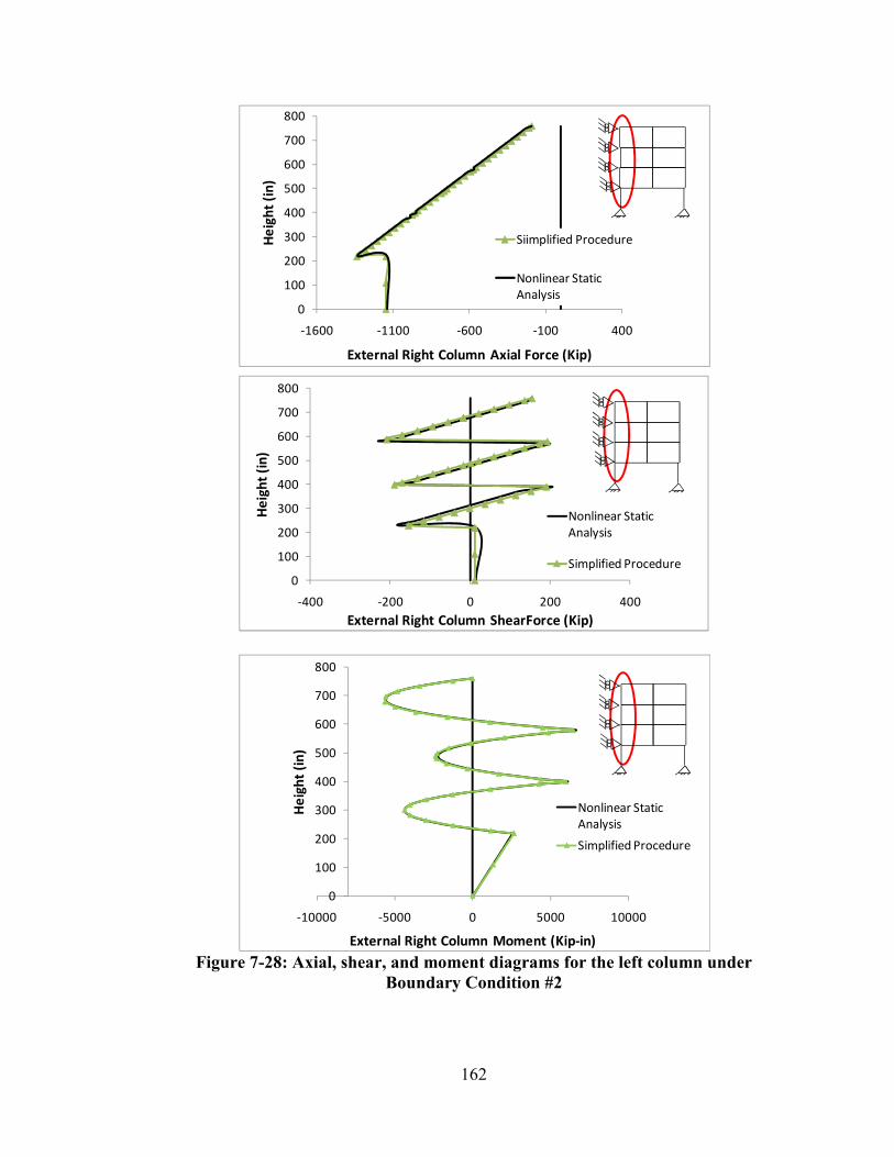
162
Figure 7-28: Axial, shear, and moment diagrams for the left column under
Boundary Condition #2
0
100
200
300
400
500
600
700
800
-1600 -1100 -600 -100 400
He
igh
t (i
n)
External Right Column Axial Force (Kip)
Siimplified Procedure
Nonlinear Static
Analysis
0
100
200
300
400
500
600
700
800
-400 -200 0 200 400
He
igh
t (i
n)
External Right Column ShearForce (Kip)
Nonlinear Static
Analysis
Simplified Procedure
0
100
200
300
400
500
600
700
800
-10000 -5000 0 5000 10000
He
igh
t (i
n)
External Right Column Moment (Kip-in)
Nonlinear Static
Analysis
Simplified Procedure
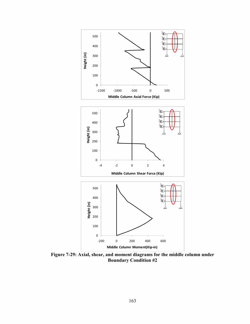
163
Figure 7-29: Axial, shear, and moment diagrams for the middle column under
Boundary Condition #2
0
100
200
300
400
500
-1500 -1000 -500 0 500
He
igh
t (i
n)
Middle Column Axial Force (Kip)
0
100
200
300
400
500
-4 -2 0 2 4
He
igh
t (i
n)
Middle Column Shear Force (Kip)
0
100
200
300
400
500
-200 0 200 400 600
He
igh
t (i
n)
Middle Column Moment(Kip-in)
164
7.4.2.3 Boundary Condition #3
Similar to Boundary Conditions #1 and 2, Boundary Condition #3 takes into account the
loss of the interior column. In addition, sidesway is inhibited on both sides of the frame.
This boundary condition results in the development of catenary actions in all beams.
Therefore, the FBD in Figure 7-24(b) is utilized to quantify the demands on exterior
columns. Due to symmetry; only the exterior column on the right side of the frame was
investigated. Figure 7-30 shows the demand distributions in this column. As shown, the
simplified procedure and the nonlinear static analysis produce similar results. For the
interior column which is damaged at the bottom story, results from the nonlinear static
analysis are presented in Figure 7-31.
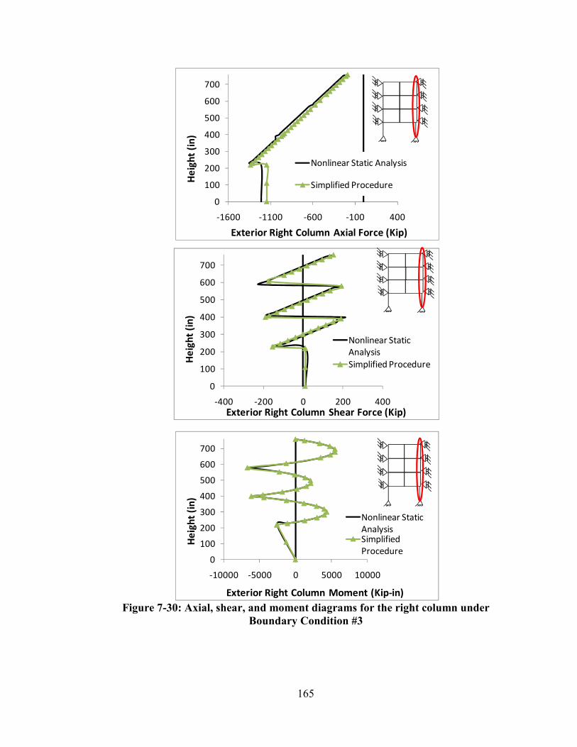
165
Figure 7-30: Axial, shear, and moment diagrams for the right column under
Boundary Condition #3
0
100
200
300
400
500
600
700
-1600 -1100 -600 -100 400
He
igh
t (i
n)
Exterior Right Column Axial Force (Kip)
Nonlinear Static Analysis
Simplified Procedure
0
100
200
300
400
500
600
700
-400 -200 0 200 400
He
igh
t (i
n)
Exterior Right Column Shear Force (Kip)
Nonlinear Static
Analysis
Simplified Procedure
0
100
200
300
400
500
600
700
-10000 -5000 0 5000 10000
He
igh
t (i
n)
Exterior Right Column Moment (Kip-in)
Nonlinear Static
AnalysisSimplified
Procedure
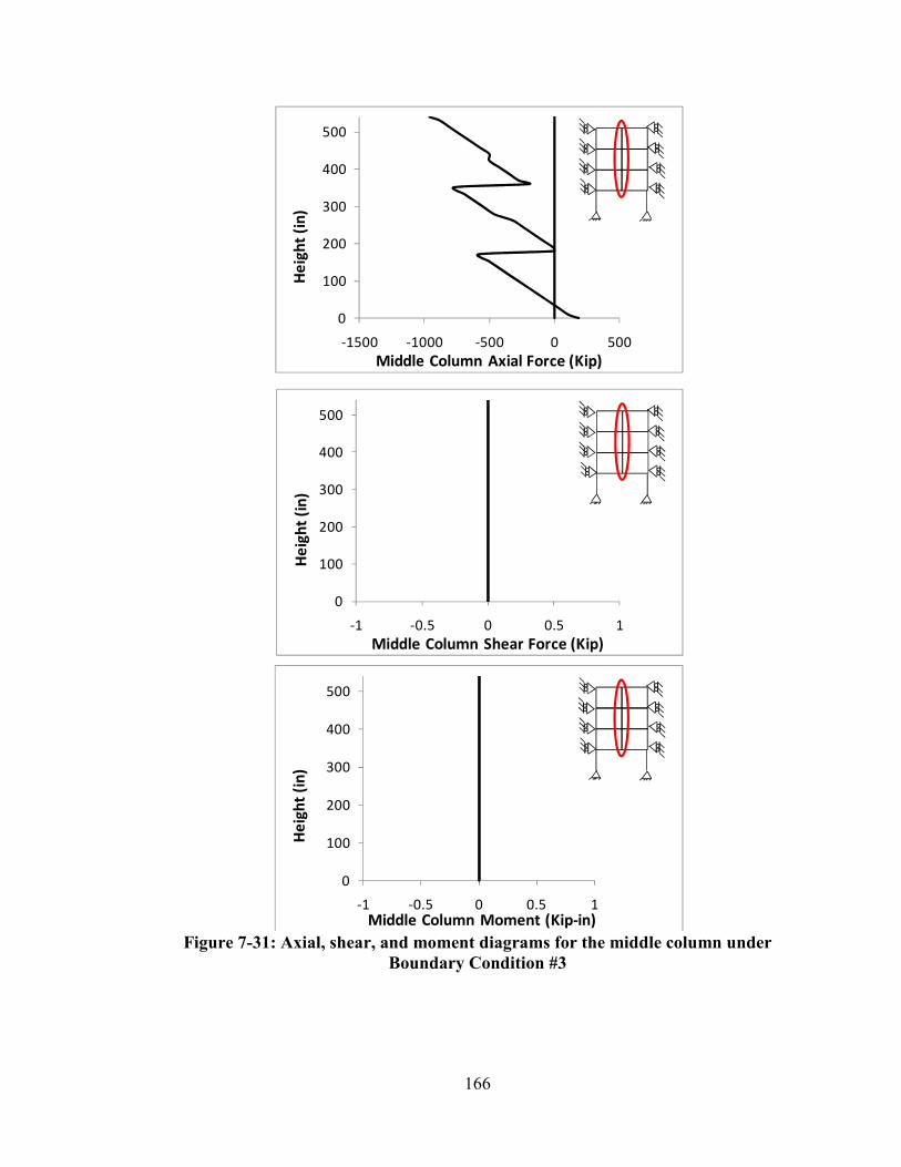
166
Figure 7-31: Axial, shear, and moment diagrams for the middle column under
Boundary Condition #3
0
100
200
300
400
500
-1500 -1000 -500 0 500
He
igh
t (i
n)
Middle Column Axial Force (Kip)
0
100
200
300
400
500
-1 -0.5 0 0.5 1
He
igh
t (i
n)
Middle Column Shear Force (Kip)
0
100
200
300
400
500
-1 -0.5 0 0.5 1
He
igh
t (i
n)
Middle Column Moment (Kip-in)
167
7.4.2.4 Boundary Condition #4
Boundary Condition #4 considers the loss of an exterior column at the bottom story and
allows sidesway displacement of the frame. The FBD shown in Figure 7-24(a) was used
to calculate the demands in the left exterior column and the corresponding results are
compared with those from the nonlinear static analysis in Figure 7-32. As shown, results
from the simplified procedure agree well with those from the nonlinear static analysis.
In addition to the left exterior column, the right exterior column and the interior column
were analyzed. It should be noted that the tension field actions develop completely in the
right bay of the frame; however, incompletely in the left bay of the frame. Therefore, the
FBDs cannot be used for these two columns and only the nonlinear static analysis was
conducted. Detailed results are presented in Figure 7-33 and Figure 7-34, respectively.
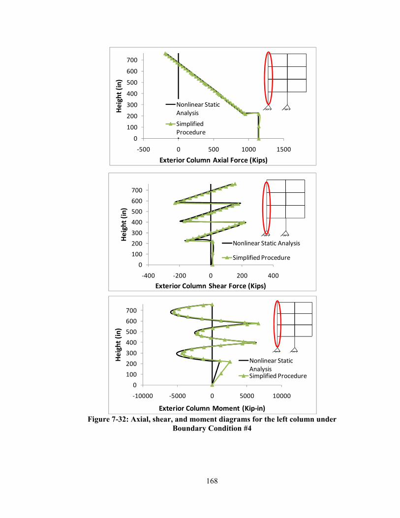
168
Figure 7-32: Axial, shear, and moment diagrams for the left column under
Boundary Condition #4
0
100
200
300
400
500
600
700
-500 0 500 1000 1500
He
igh
t (i
n)
Exterior Column Axial Force (Kips)
Nonlinear Static
Analysis
Simplified
Procedure
0
100
200
300
400
500
600
700
-400 -200 0 200 400
He
igh
t (i
n)
Exterior Column Shear Force (Kips)
Nonlinear Static Analysis
Simplified Procedure
0
100
200
300
400
500
600
700
-10000 -5000 0 5000 10000
He
igh
t (i
n)
Exterior Column Moment (Kip-in)
Nonlinear Static
AnalysisSimplified Procedure
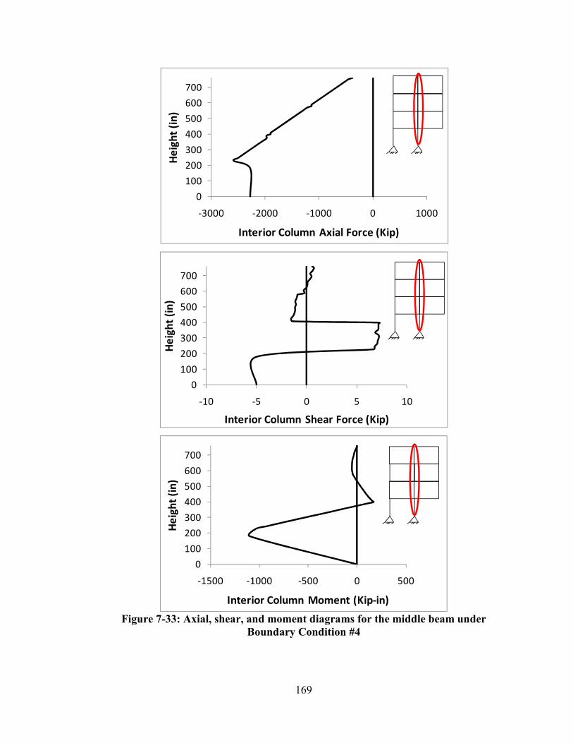
169
Figure 7-33: Axial, shear, and moment diagrams for the middle beam under
Boundary Condition #4
0
100
200
300
400
500
600
700
-3000 -2000 -1000 0 1000
He
igh
t (i
n)
Interior Column Axial Force (Kip)
0
100
200
300
400
500
600
700
-10 -5 0 5 10
He
igh
t (i
n)
Interior Column Shear Force (Kip)
0
100
200
300
400
500
600
700
-1500 -1000 -500 0 500
He
igh
t (i
n)
Interior Column Moment (Kip-in)

170
Figure 7-34: Axial, shear, and moment diagrams for the right column under
Boundary Condition #4
0
100
200
300
400
500
-600 -400 -200 0 200
He
igh
t (i
n)
Column Axial Force (Kip)
0
100
200
300
400
500
-400 -200 0 200 400
He
igh
t (i
n)
Column Shear Force (Kip)
Nonlinear
Static
Analysis
0
100
200
300
400
500
-10000 -5000 0 5000 10000
He
igh
t (i
n)
Column Moment (Kip-in)
Nonlinear
Static Analysis
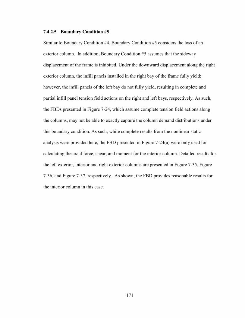
171
7.4.2.5 Boundary Condition #5
Similar to Boundary Condition #4, Boundary Condition #5 considers the loss of an
exterior column. In addition, Boundary Condition #5 assumes that the sideway
displacement of the frame is inhibited. Under the downward displacement along the right
exterior column, the infill panels installed in the right bay of the frame fully yield;
however, the infill panels of the left bay do not fully yield, resulting in complete and
partial infill panel tension field actions on the right and left bays, respectively. As such,
the FBDs presented in Figure 7-24, which assume complete tension field actions along
the columns, may not be able to exactly capture the column demand distributions under
this boundary condition. As such, while complete results from the nonlinear static
analysis were provided here, the FBD presented in Figure 7-24(a) were only used for
calculating the axial force, shear, and moment for the interior column. Detailed results for
the left exterior, interior and right exterior columns are presented in Figure 7-35, Figure
7-36, and Figure 7-37, respectively. As shown, the FBD provides reasonable results for
the interior column in this case.

172
Figure 7-35: Axial, shear, and moment diagrams for the left column under
Boundary Condition #5
0
100
200
300
400
500
600
700
-300 -200 -100 0 100
He
igh
t (i
n)
Exterior Column Axial Force (Kips)
0
100
200
300
400
500
600
700
-100 -50 0 50 100
He
igh
t (i
n)
Exterior Column Shear Force (Kips)
0
100
200
300
400
500
600
700
-2000 0 2000
He
igh
t (i
n)
Exterior Column Moment (Kips-in)
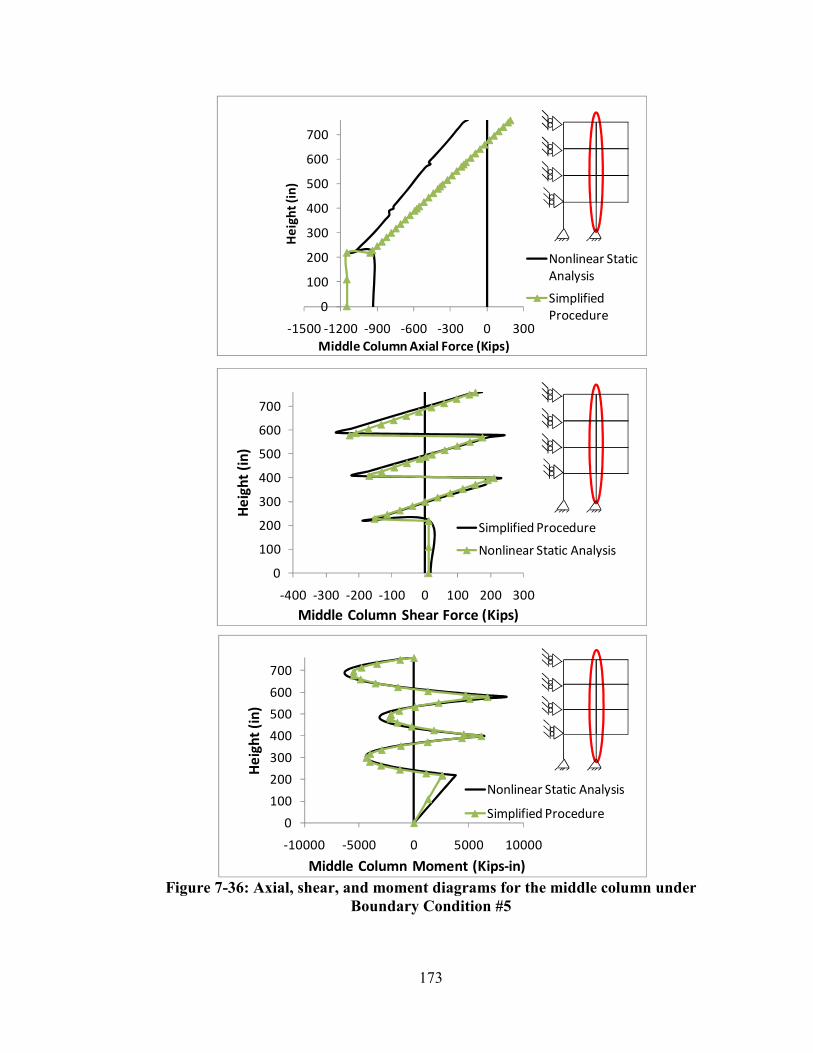
173
Figure 7-36: Axial, shear, and moment diagrams for the middle column under
Boundary Condition #5
0
100
200
300
400
500
600
700
-1500 -1200 -900 -600 -300 0 300
He
igh
t (i
n)
Middle Column Axial Force (Kips)
Nonlinear Static
Analysis
Simplified
Procedure
0
100
200
300
400
500
600
700
-400 -300 -200 -100 0 100 200 300
He
igh
t (i
n)
Middle Column Shear Force (Kips)
Simplified Procedure
Nonlinear Static Analysis
0
100
200
300
400
500
600
700
-10000 -5000 0 5000 10000
He
igh
t (i
n)
Middle Column Moment (Kips-in)
Nonlinear Static Analysis
Simplified Procedure

174
Figure 7-37: Axial, shear, and moment diagrams for the right column under
Boundary Condition #5
7.5 Summary
The demands on the boundary frame members (i.e. beams and columns) were
investigated in this chapter. All five boundary conditions presented in Figure 5-1 were
considered. The demands obtained respectively from the nonlinear static analysis using
0
100
200
300
400
500
-600 -400 -200 0 200
He
igh
t (i
n)
Exterior Column Axial Force (Kips)
0
100
200
300
400
500
-400 -200 0 200 400
He
igh
t (i
n)
Exterior Column Shear (Kips)
Nonlinear Static
Analysis
0
100
200
300
400
500
-10000 -5000 0 5000 10000
He
igh
t (i
n)
Exterior Column Moment (Kips-in)
Nonlinear Static
Analysis

175
the 2D FE models and the simplified procedure using the developed FBDs were
compared. It was observed that the simple FBDs adequately capture the demand
distributions along the frame members.
176
8 IMPACT OF BEAM-TO-COLUMN CONNECTION FAILURE ON SYSTEM
BEHAVIOR
8.1 Introduction
As discussed in the previous sections, beam-to-column connections play an important
role to transfer the axial forces in the beam to the adjacent columns when sudden column
failure occurs. To date, significant research efforts have been made to improve the
performance of beam-to-column connections to enhance the system progressive collapse
resistance (Li 2009).
In the proposed system, the beam-to-column connections may suffer from premature
failure for the following two reasons: 1) the deformation capacity (i.e., ductility) of the
connections may not be sufficient for fully developing the system strength; and 2)
significant tensile force may exist in the beam-to-column connections when the frame
boundary conditions allow the development of catenary actions. This chapter
investigates how the progressive collapse resistance of the proposed system will be
affected when premature failure occurs in the beam-to-column connections.
The 3D FE model developed in ABAQUS and considered in Chapter 4 was used here for
modeling the behavior of the proposed system under connection failures. First, the
beams with connection failures were partitioned into three segments: two exterior
segments and one interior segment, which represent the connection elements and the
beam element, respectively. The length of each connection element is 5% of the original
beam length. The failures of the beam-to-column connections were then taken into
177
account by assigning reduced yield strength (3% of the beam yield strength) and a
reduced cross-section area (50-70% of the original beam cross-section area) to the
connection elements. The progressive collapse resistances of the retrofitted system with
and without beam-to-column failure are then compared to quantify the impact of
connection failures.
Additionally, the system strength with connection failures is estimated using the
following equation:
3
1
1 1sin 2 ( )
2 2i
n
y pt
i
P f h t b c A Eα θ=
= ⋅ ⋅ ⋅ + − ⋅ ⋅ ⋅ ⋅
∑ (8-1)
where, c = number of beams affected by connection failures; and all other variables have
been previously defined.
Note that the above equation is based on equation (3-59), which was derived based on
plastic analysis. Additionally, it takes into account the loss of beam catenary actions due
to the beam-to-column connection failures.
Given that the beam-to-column connections may be more vulnerable to failure when
large tensile forces caused by the catenary action develop in the beams, the system under
Boundary Condition #3 (which assumes sideway inhibited boundary conditions on both
sides of the frame and allow the development of the beam catenary actions) was selected
for investigation.
178
8.2 Case Studies
This section investigates the impact of connection failure on the behavior of the proposed
system under Boundary Condition #3. For comparison purpose, a total of four cases (i.e.
Cases A through D, see Table 8-1 for detailed information) were considered here to
investigate the impacts of 1) connection failures occurring at different locations and 2)
number of connection failures. Detailed results from Cases A through D are presented
below.
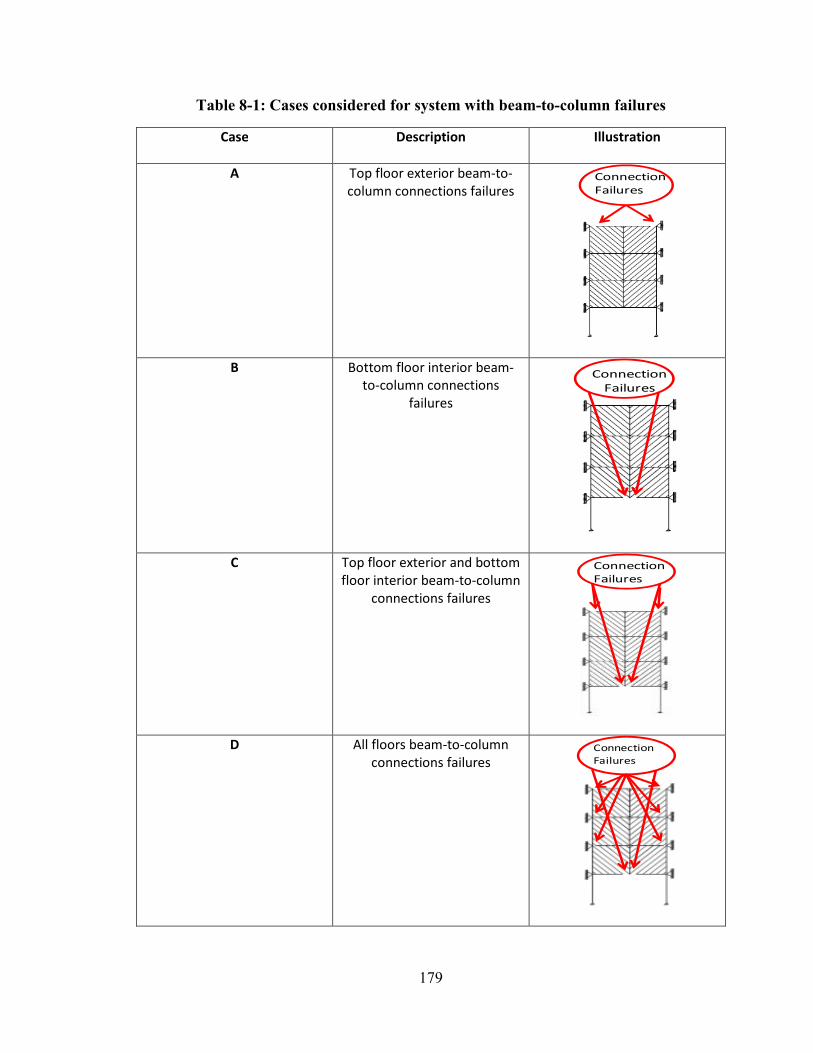
179
Table 8-1: Cases considered for system with beam-to-column failures
Case Description Illustration
A Top floor exterior beam-to-
column connections failures
B Bottom floor interior beam-
to-column connections
failures
C Top floor exterior and bottom
floor interior beam-to-column
connections failures
D All floors beam-to-column
connections failures
Connection
Failures
Connection
Failures
Connection
Failures
Connection
Failures
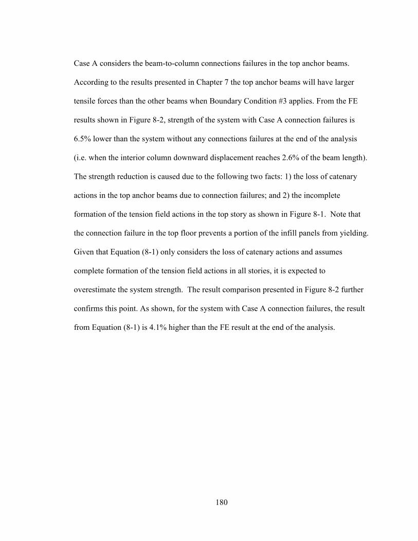
180
Case A considers the beam-to-column connections failures in the top anchor beams.
According to the results presented in Chapter 7 the top anchor beams will have larger
tensile forces than the other beams when Boundary Condition #3 applies. From the FE
results shown in Figure 8-2, strength of the system with Case A connection failures is
6.5% lower than the system without any connections failures at the end of the analysis
(i.e. when the interior column downward displacement reaches 2.6% of the beam length).
The strength reduction is caused due to the following two facts: 1) the loss of catenary
actions in the top anchor beams due to connection failures; and 2) the incomplete
formation of the tension field actions in the top story as shown in Figure 8-1. Note that
the connection failure in the top floor prevents a portion of the infill panels from yielding.
Given that Equation (8-1) only considers the loss of catenary actions and assumes
complete formation of the tension field actions in all stories, it is expected to
overestimate the system strength. The result comparison presented in Figure 8-2 further
confirms this point. As shown, for the system with Case A connection failures, the result
from Equation (8-1) is 4.1% higher than the FE result at the end of the analysis.

181
Figure 8-1: Tension field action distribution in the frame under Boundary
Condition #3 and Case A connection failures
Elastic
Yielded
Yielded
Yielded
Elastic
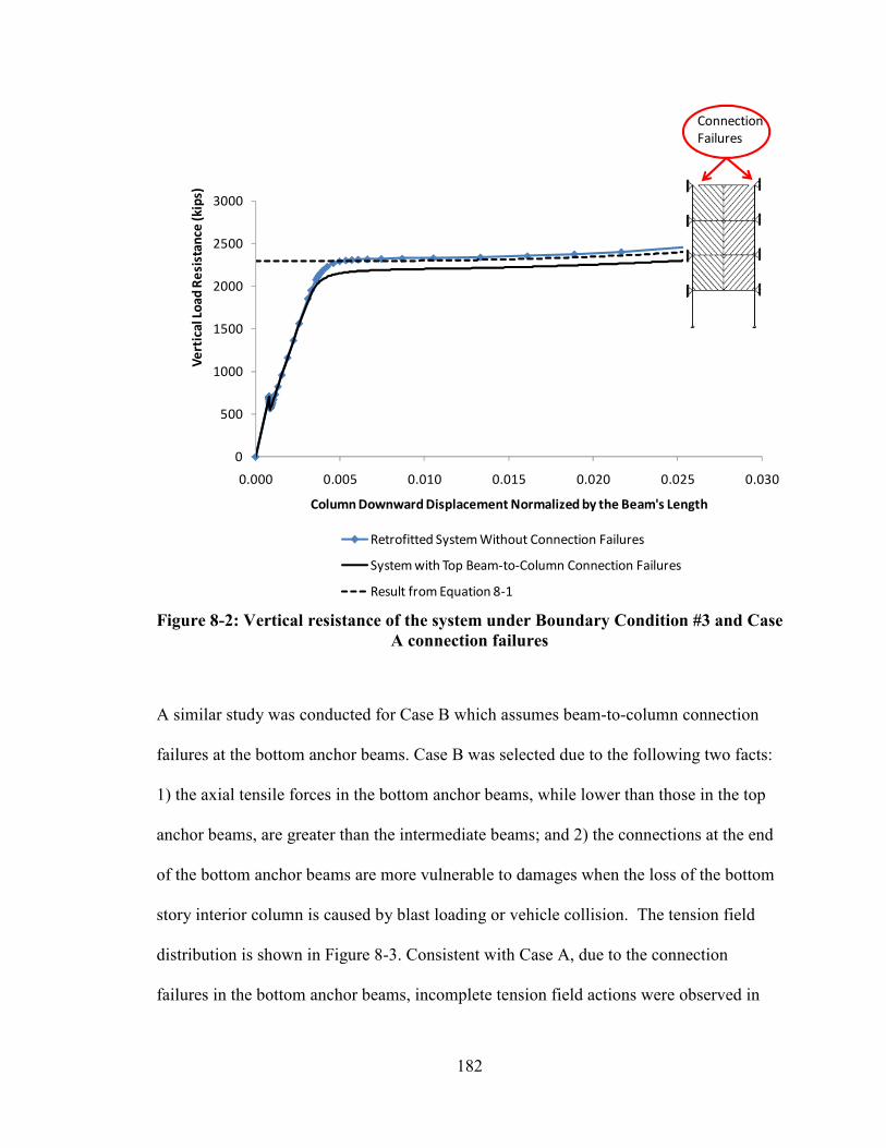
182
Figure 8-2: Vertical resistance of the system under Boundary Condition #3 and Case
A connection failures
A similar study was conducted for Case B which assumes beam-to-column connection
failures at the bottom anchor beams. Case B was selected due to the following two facts:
1) the axial tensile forces in the bottom anchor beams, while lower than those in the top
anchor beams, are greater than the intermediate beams; and 2) the connections at the end
of the bottom anchor beams are more vulnerable to damages when the loss of the bottom
story interior column is caused by blast loading or vehicle collision. The tension field
distribution is shown in Figure 8-3. Consistent with Case A, due to the connection
failures in the bottom anchor beams, incomplete tension field actions were observed in
0
500
1000
1500
2000
2500
3000
0.000 0.005 0.010 0.015 0.020 0.025 0.030
Ve
rtic
al L
oa
d R
esi
sta
nce
(k
ips)
Column Downward Displacement Normalized by the Beam's Length
Retrofitted System Without Connection Failures
System with Top Beam-to-Column Connection Failures
Result from Equation 8-1
Connection
Failures
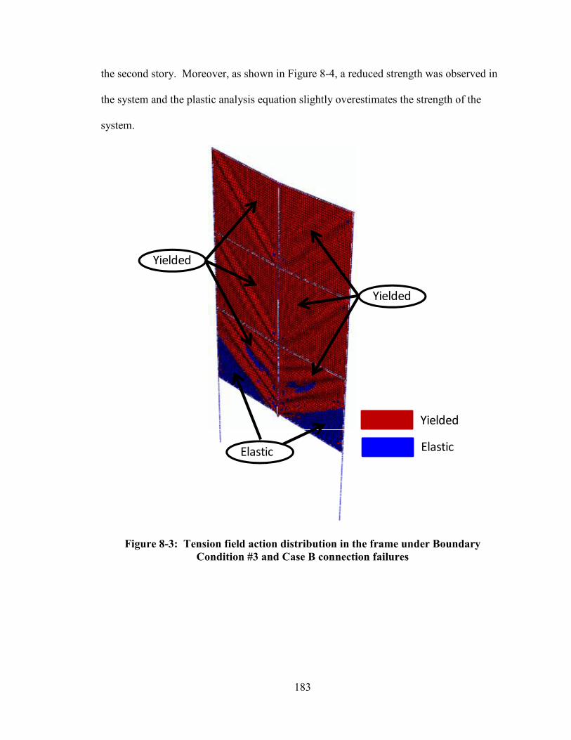
183
the second story. Moreover, as shown in Figure 8-4, a reduced strength was observed in
the system and the plastic analysis equation slightly overestimates the strength of the
system.
Figure 8-3: Tension field action distribution in the frame under Boundary
Condition #3 and Case B connection failures
Elastic
Yielded
Yielded
Yielded
Elastic
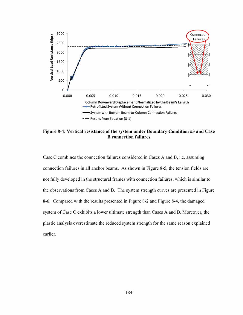
184
Figure 8-4: Vertical resistance of the system under Boundary Condition #3 and Case
B connection failures
Case C combines the connection failures considered in Cases A and B, i.e. assuming
connection failures in all anchor beams. As shown in Figure 8-5, the tension fields are
not fully developed in the structural frames with connection failures, which is similar to
the observations from Cases A and B. The system strength curves are presented in Figure
8-6. Compared with the results presented in Figure 8-2 and Figure 8-4, the damaged
system of Case C exhibits a lower ultimate strength than Cases A and B. Moreover, the
plastic analysis overestimate the reduced system strength for the same reason explained
earlier.
0
500
1000
1500
2000
2500
3000
0.000 0.005 0.010 0.015 0.020 0.025 0.030
Ve
rtic
al L
oa
d R
esi
sta
nce
(k
ips)
Column Downward Displacement Normalized by the Beam's Length
Retrofitted System Without Connection Failures
System with Bottom Beam-to-Column Connection Failures
Results from Equation (8-1)
Connection
Failures
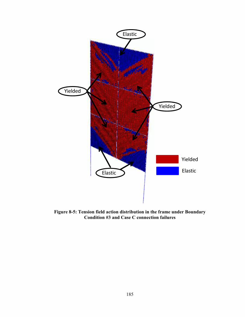
185
Figure 8-5: Tension field action distribution in the frame under Boundary
Condition #3 and Case C connection failures
Elastic
Elastic
Yielded
Yielded
Yielded
Elastic

186
Figure 8-6: Vertical resistance of the system under Boundary Condition #3 and Case
C connection failures
Case D considers the worst scenario in which connection failures occurs in all beam
members. The locations where connection failures occur are given in Figure 8-8 together
with the system responses. Compared with Cases A to C, the system considered in Case
D has a lower vertical load resistance due to the loss of catenary action in all beams and
the absence of complete tension field actions. The plate yielding distribution is shown in
Figure 8-7. It is observed that the tension field distribution of Case D is similar to that of
Case C, indicating that connections failures in intermediate beams have a negligible
impact on development of tension field actions when plates with identical thickness and
strength are used in all stories. Similar to the prior cases, the plastic analysis procedure
produces an overestimate of the system strength.
0
500
1000
1500
2000
2500
3000
0.000 0.005 0.010 0.015 0.020 0.025 0.030
Ve
rtic
al Lo
ad
Re
sist
an
ce
(k
ips)
Column Downward Displacement Normalized by the Beam's Length
Retrofitted System Without Connection Failures
System with Top and Bottom Anchor Beam-to-Column Connection Failures
Results from Equation (8-1)
Connection
Failures
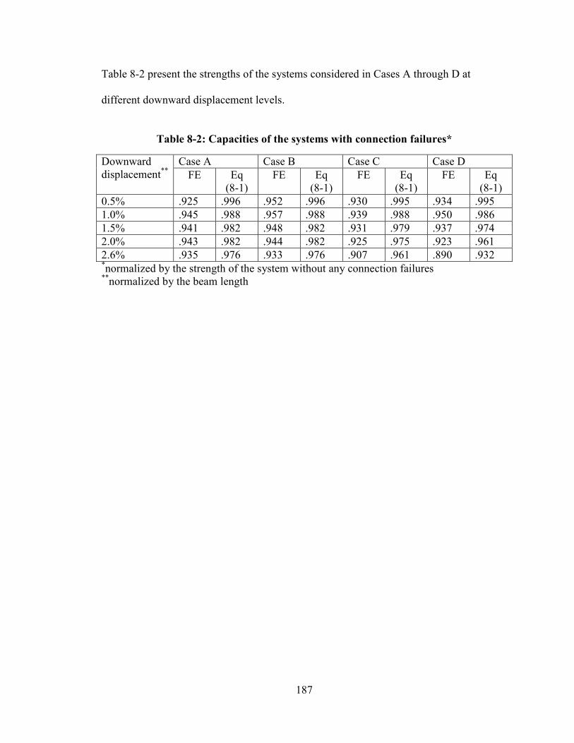
187
Table 8-2 present the strengths of the systems considered in Cases A through D at
different downward displacement levels.
Table 8-2: Capacities of the systems with connection failures*
Downward
displacement**
Case A Case B Case C Case D
FE Eq
(8-1)
FE Eq
(8-1)
FE Eq
(8-1)
FE Eq
(8-1)
0.5% .925 .996 .952 .996 .930 .995 .934 .995
1.0% .945 .988 .957 .988 .939 .988 .950 .986
1.5% .941 .982 .948 .982 .931 .979 .937 .974
2.0% .943 .982 .944 .982 .925 .975 .923 .961
2.6% .935 .976 .933 .976 .907 .961 .890 .932 *normalized by the strength of the system without any connection failures
**normalized by the beam length
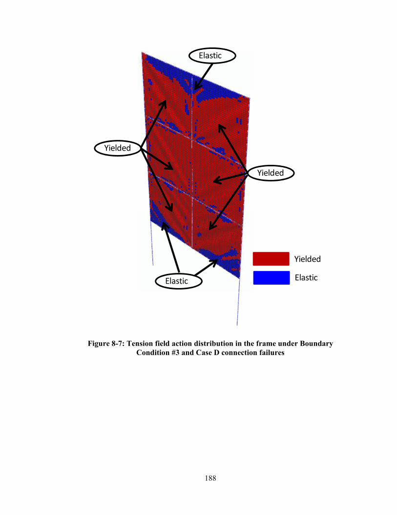
188
Figure 8-7: Tension field action distribution in the frame under Boundary
Condition #3 and Case D connection failures
Elastic
Elastic
Yielded
Yielded
Yielded
Elastic
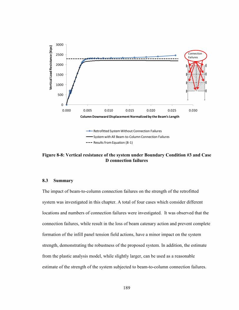
189
Figure 8-8: Vertical resistance of the system under Boundary Condition #3 and Case
D connection failures
8.3 Summary
The impact of beam-to-column connection failures on the strength of the retrofitted
system was investigated in this chapter. A total of four cases which consider different
locations and numbers of connection failures were investigated. It was observed that the
connection failures, while result in the loss of beam catenary action and prevent complete
formation of the infill panel tension field actions, have a minor impact on the system
strength, demonstrating the robustness of the proposed system. In addition, the estimate
from the plastic analysis model, while slightly larger, can be used as a reasonable
estimate of the strength of the system subjected to beam-to-column connection failures.
0
500
1000
1500
2000
2500
3000
0.000 0.005 0.010 0.015 0.020 0.025 0.030
Ve
rtic
al L
oa
d R
esi
sta
nce
(k
ips)
Column Downward Displacement Normalized by the Beam's Length
Retrofitted System Without Connection Failures
System with All Beam-to-Column Connection Failures
Results from Equation (8-1)
Connection
Failures

190
9 SUMMARY, CONCLUSIONS, AND RECOMMENDATIONS FOR FUTURE
RESEARCH
9.1 Summary and Conclusions
This thesis investigated the potential use of thin infill panels in steel frames for
enhancement of the system’s progressive collapse resistance. Five boundary conditions
were examined to consider the impacts of the different locations of initial column failures
and the different lateral displacement restraints on both sides of the frame. Three
analytical models were developed. The first model was based on plastic analysis theory.
The second and third models are FE models requiring different levels of modeling efforts.
Performance of the proposed system was evaluated using all the three developed models.
In addition, the system performance obtained from nonlinear static FE analysis was
modified to take into account the dynamic effects of progressive collapse. Furthermore,
simple FBDs for quantifying the demands including axial force, shear force and bending
moment on the boundary frame members were developed. Last, the impact of premature
beam-to-column connection failures on the system progressive collapse resistance was
addressed.
Through the analytical work conducted in this research, the following conclusions may
be drawn:
1. the proposed system is effective to enhance the system progressive collapse
resistance under all the considered boundary conditions.
2. all the developed analytical models are effective for calculating the system
ultimate strength. The plastic model is very simple and can be used in hand

191
calculations for preliminary design of the plate thickness. The 3D FE model can
be used for capturing the plate buckling and other local component behaviors.
The 2D FE model can be used for a better determination of demand distributions
in the boundary frame members.
3. the dynamic effects can be considered by modifying the system response
obtained from the nonlinear static FE analysis.
4. the demands on boundary frame members can be calculated using the developed
simple FBDs.
5. the proposed system is very robust and exhibits stable progressive collapse
resistance even when premature beam-to-column connection failures occur in the
system.
9.2 Recommendations for Future Research
While the dynamic effects were indirectly considered in Chapter 7, it would be
interesting to explore the actual dynamic behavior of the proposed system through
nonlinear dynamic analysis.
In addition, this thesis only considered simple beam-to-column connections. It would be
beneficial to investigate the behavior of the proposed system when the beam-to-column
connections are fully rigid.
Furthermore, this thesis assumed either ideally rigid or ideally flexible lateral boundary
conditions (i.e., either sidesway inhibited or sidesway uninhibited); it would be

192
interesting to investigate the performance of the proposed system when the stiffness of
the lateral restraints varies over a practical range.
193
REFERENCES
ACI. Building code Requirements for Structural Concrete (ACI Standard 318-08).
Farmington Hills, MI: American Concrete Institute, 2008.
AISC. (2005). “American Institute of Steel Construction.” Chicago, Illinois.
ASCE Standard 7-05, Minimum Design Loads for Buildings and Other Structures
(ASCE/SEI 7-2005) (2005), American Society of Civil Engineers, Reston, VA.
Astaneh-Asl, A. “Progressive Collapse Prevention of Steel Frames with Shear
Connections.” Department of Civil and Environmental Engineering and Center for
Catastrophic Risk Management University of California, Berkeley, 2007.
Astaneh-Asl, A, D. McCallen, E. Madsen, and C. Noble (2001) “Experimental and
Analytical Studies of Floor Catenary Action to Prevent Progressive Collapse,” Report
Number UCB/CESteel-01/03, Department of Civil and Environmental Engineering,
University of California, Berkeley, December (www.ce.berkeley.edu/~astaneh).
Behbahanifard, M. R., Grondin, G. Y., and Elwi, A. E. (2003). “Experimental and
Numerical Investigation of Steel Plate Shear Wall.” Structural Engineering Report 254,
Department of Civil Engineering, University of Alberta, Edmonton, Alberta, Canada.
Berman, J. W. and Bruneau, M. (2003), “Experimental Investigation of Light-Gauge
Steel Plate Shear Walls for the Seismic Retrofit Of Buildings.” Technical Report
MCEER-03-0001, Multidisciplinary Center for Earthquake Engineering Research,
Buffalo, N.Y., May 2, 2003.
Berman, J. W., and Bruneau, M. (2008), “Capacity Design of Vertical Boundary
Elements in Steel Plate Shear Walls.” AISC Engineering Journal Vol.45, No.1., pp.57-71.
Cleland, N.M. “Containing Progressive Collapse in Precast Concrete Systems.” ASCENT,
Summer 2007.
DoD. Design of Buildings to Resist Progressive Collapse (UFC 4-023-03). Washington,
DC: United States Department of Defense, 2009.
Driver, R. G., Kulak, G. L., Kennedy, D. J. L., and Elwi, A. E. (1997). “Seismic Behavior
of Steel Plate Shear Walls.” Structural Engineering Report 215, Department of Civil
Engineering, University of Alberta, Edmonton, Alberta, Canada.
Federal Emergency Management Agency (FEMA 403). (2002). “World Trade Center
building performance study: Data collection, preliminary observations, and
recommendations.” <http://www.fema.gov/rebuild/mat/mat_fema403.shtm>(January,
2011)

194
Federal Emergency Management Agency (FEMA 450). (2004), "NEHRP Recommended
Provisions For Seismic Regulations For New Buildings And Other Structures." Building
Seismic Safety Council for the Federal Emergency Management Agency, Washington,
D.C.
Hibbitt, Karlsson, and Sorenson, Inc. (HKS) (2009), "ABAQUS/Standard Users
Manual.” Version 6.9, Hibbitt, Karlsson, and Sorenson, Inc., Pawtucket, Rhode Island.
Hoffman S. T. (2010) “Behavior and performance of steel moment-framed buildings
subject to dynamic column loss scenarios” Master Thesis, University of Illinois at Urbana
Champaign. 2010.
Izzuddin B.A. “Ductility assessment for an idealized elasto-Plastic structural system
subject to an instantaneous applied load.” Internal discussion document. Imperial College
London (UK). 2004.
Izzuddin B.A., Vlassis A.G., Elghazouli A.Y., Nethercot D.A., "Progressive collapse of
multi-storey buildings due to sudden column loss-Part I: Simplified assessment
framework." Imperial College London (UK). 2007.
Level3.com (Sep 20, 2001) <http://mirror-uk-rb1.gallery.hd.org> "moment of collision of
flight UA175 Boeing 767 jet with south tower causing huge explosion seen from side of
entry 2 ANON.jpg" (January, 2011)
Li J.L. “Preventing progressive collapse through strengthening beam-to-column
connection, Part 1: Theoretical analysis” Journal of Constructional Steel Research 66
(2010) 229_237. September 13, 2009.
Marchand A. K., Alfawakhiri F. American Institute of Steel Construction, Inc. “Facts for
Steel Buildings-Blast and Progressive Collapse” vol. 2. USA: AISC; 2004.
Marchand A. K., Moore W. P., Alfawakhiri F. American Institute of Steel Construction,
Inc. “Facts for Steel Buildings-Blast and Progressive Collapse” 2004.
Qu, B., and Bruneau (2008), “Seismic Behavior and Design of Boundary Frame
Members in Steel Plate Shear Walls” Technical Rep. No. MCEER-08-0012,
Multidisciplinary Center for Earthquake Engineering Research, Buffalo, N.Y., June 20,
2008.
Qu, B., and Bruneau (2010), “Capacity Design of Intermediate Horizontal Boundary
Elements of Steel Plate Shear Walls” ASCE Journal of Structural Engineering, Vol. 136,
No. 6, June 1, 2010.
Simulia. Abaqus. Providence, RI: Dassault Systemes Corp., 2008.

195
Thorburn, L. Jane, Kulak, G. L., and Montgomery, C. J. (1983). “Analysis of Steel Plate
Shear Walls.” Structural Engineering Report No. 107, Department of Civil Engineering,
University of Alberta, Edmonton, Alberta, Canada.
Timler, P. A. and Kulak, G. L. (1983). “Experimental Study of Steel Plate Shear Walls.”
Structural Engineering Report No. 114, Department of Civil Engineering, University of
Alberta, Edmonton, Alberta, Canada.
Timoshenko, S.(1955). Strength of Materials New York: D. Van Nostrand Company.
Wagner, H., Flat Sheet Metal Girders with Very Thin Metal Webs. Part I—General
Theories and Assumptions, National Advisory Committee for Aeronautics, Technical
Memo No. 604, 1931
Wearne, P. (2000). Collapse: When buildings fall down, TV Books, New York
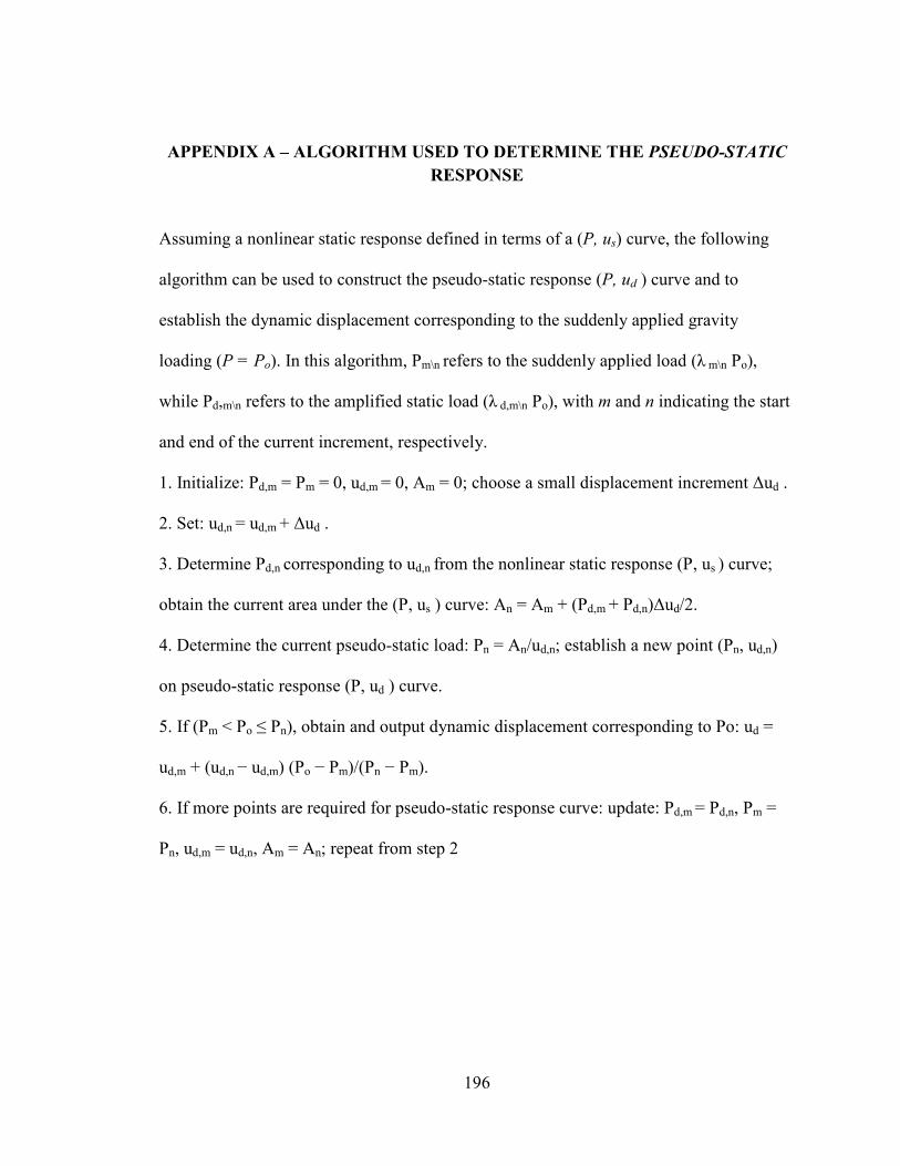
196
APPENDIX A – ALGORITHM USED TO DETERMINE THE PSEUDO-STATIC
RESPONSE
Assuming a nonlinear static response defined in terms of a (P, us) curve, the following
algorithm can be used to construct the pseudo-static response (P, ud ) curve and to
establish the dynamic displacement corresponding to the suddenly applied gravity
loading (P = Po). In this algorithm, Pm\n refers to the suddenly applied load (λ m\n Po),
while Pd,m\n refers to the amplified static load (λ d,m\n Po), with m and n indicating the start
and end of the current increment, respectively.
1. Initialize: Pd,m = Pm = 0, ud,m = 0, Am = 0; choose a small displacement increment ∆ud .
2. Set: ud,n = ud,m + ∆ud .
3. Determine Pd,n corresponding to ud,n from the nonlinear static response (P, us ) curve;
obtain the current area under the (P, us ) curve: An = Am + (Pd,m + Pd,n)∆ud/2.
4. Determine the current pseudo-static load: Pn = An/ud,n; establish a new point (Pn, ud,n)
on pseudo-static response (P, ud ) curve.
5. If (Pm < Po ≤ Pn), obtain and output dynamic displacement corresponding to Po: ud =
ud,m + (ud,n − ud,m) (Po − Pm)/(Pn − Pm).
6. If more points are required for pseudo-static response curve: update: Pd,m = Pd,n, Pm =
Pn, ud,m = ud,n, Am = An; repeat from step 2
Related Documents