Engineering Sensorial Delay to Control Phototaxis and Emergent ...yoksis.bilkent.edu.tr/pdf/files/12654.pdf · Engineering Sensorial Delay to Control Phototaxis and Emergent Collective

Engineering Sensorial Delay to Control Phototaxis and Emergent Collective Behaviors

Mite Mijalkov,1,2 Austin McDaniel,3 Jan Wehr,3 and Giovanni Volpe1,21Soft Matter Lab, Department of Physics, Bilkent University, Cankaya, 06800 Ankara, Turkey2UNAM-National Nanotechnology Research Center, Bilkent University, Ankara 06800, Turkey

3Department of Mathematics and Program in Applied Mathematics,University of Arizona, Tucson, Arizona 85721, USA

(Received 7 September 2015; published 29 January 2016)

Collective motions emerging from the interaction of autonomous mobile individuals play a key role inmany phenomena, from the growth of bacterial colonies to the coordination of robotic swarms. For thesecollective behaviors to takehold, the individualsmust be able to emit, sense, and react to signals.Whendealingwith simple organisms and robots, these signals are necessarily very elementary; e.g., a cell might signal itspresence by releasing chemicals and a robot by shining light. An additional challenge arises because themotion of the individuals is often noisy; e.g., the orientation of cells can be altered by Brownian motion andthat of robots by an uneven terrain. Therefore, the emphasis is on achieving complex and tunable behaviorsfrom simple autonomous agents communicatingwith each other in robust ways. Here, we show that the delaybetween sensing and reacting to a signal can determine the individual and collective long-term behavior ofautonomous agents whose motion is intrinsically noisy. We experimentally demonstrate that the collectivebehavior of a group of phototactic robots capable of emitting a radially decaying light field can be tuned fromsegregation to aggregation and clustering by controlling the delay with which they change their propulsionspeed in response to the light intensity theymeasure.We track this transition to the underlying dynamics of thissystem, in particular, to the ratio between the robots’ sensorial delay time and the characteristic time of therobots’ random reorientation. Supported by numerics, we discuss how the same mechanism can be appliedto control active agents, e.g., airborne drones, moving in a three-dimensional space. Given the simplicity ofthis mechanism, the engineering of sensorial delay provides a potentially powerful tool to engineer anddynamically tune the behavior of large ensembles of autonomousmobile agents; furthermore, thismechanismmight already be at work within living organisms such as chemotactic cells.

DOI: 10.1103/PhysRevX.6.011008 Subject Areas: Interdisciplinary Physics, Soft Matter

I. INTRODUCTION

The interaction between several simple autonomousagents can give rise to complex collective behaviors.This is observed at all scales, from the organization ofbacterial colonies [1,2] and the foraging of ants and bees [3]to the assembly of schools of fish [4] and the collectivemotion of human crowds [5]. Inspired by these naturalsystems, the same principles have been applied to engineerautonomous robots capable of performing tasks such assearch-and-rescue in disaster zones, surveillance of haz-ardous areas, and targeted object delivery in complexenvironments [6–11].Complex behaviors can emerge even if each agent follows

very simple rules, senses only its immediate surroundings,and directly interacts only with nearby agents, withouthaving any knowledge of an overall plan [12,13]. Forexample, while performing their swim-and-tumble motion,

chemotactic bacteria are able to climba chemotactic gradient,e.g., in order to move towards regions rich in nutrients,by simply adjusting their tumbling rate depending on thechemical concentration they sense [2,14]. Furthermore, byreleasing chemoattractant molecules into their surroundings,they are capable of generating a chemical gradient aroundthemselves to which other cells can respond, e.g., in order tocreate bacterial colonies [1]. Similarly, simple mechanismsare at work in the organization of flocks of birds, schools offish, and herds of mammals, whereby complex collectivebehaviors result from each animal reacting to signals sent byits neighbors. A similar approach has also been fruitfullyexplored in order to build artificial systems with robustbehaviors arising from interactions between very simpleconstituent agents [6,10,11,15–18]. Complex behaviorsemerging from agents obeying simple rules have the advan-tage of being extremely robust: For example, even if one ormore agents are destroyed, the others can continue to worktogether to complete the task at hand; agents can also beremoved or addedmidtaskwithout significantly affecting thefinal result.Here, we experimentally and theoretically demonstrate

that it is possible to engineer the individual and collective

Published by the American Physical Society under the terms ofthe Creative Commons Attribution 3.0 License. Further distri-bution of this work must maintain attribution to the author(s) andthe published article’s title, journal citation, and DOI.

PHYSICAL REVIEW X 6, 011008 (2016)

2160-3308=16=6(1)=011008(16) 011008-1 Published by the American Physical Society

behavior of autonomous agents whose motion is intrinsi-cally noisy by making use of the delay in their sensorialfeedback cycle. In other words, we show how the delaybetween the time when an agent senses a signal and thetime when it reacts to it can be used as a new parameter forthe engineering of large-scale organization of autonomousagents. This proposal is inspired by the motion of chemo-tactic cells, which are able to climb a chemical gradient byadjusting a different parameter, i.e., their tumbling rate, inresponse to the concentration of molecules in their sur-roundings. We demonstrate that the collective behavior of agroup of phototactic robots, capable of emitting a radiallydecaying light field, can be tuned from segregation toaggregation and clustering by controlling the delay withwhich they adjust their propulsion speed to the lightintensity. More precisely, we show that this transitionoccurs as the ratio between the robots’ sensorial delaytime and characteristic time of their random reorientationcrosses a certain critical value.

II. SINGLE AGENT

We start by considering a single autonomous agent thatmoves in a plane and whose orientation is subject to noise.This happens naturally in the case of microswimmers—microscopic particles capable of self-propulsion such asmotile bacteria and cells [19,20]—as the direction of theirmotion changes randomly over time because of the pres-ence of rotational Brownian motion [2]. Similarly, autono-mous robots, animals, and even humans can undergo arandom reorientation when moving in the absence ofexternal reference points (a striking example of this is anexperiment where blindfolded people who were asked towalk in a straight line spontaneously moved along benttrajectories [21]). Such motion is known as activeBrownian motion and can be modeled by the followingsystem of stochastic differential equations [12,20,22,23]:

8>>><>>>:

dxtdt ¼ v cosϕt;dytdt ¼ v sinϕt;

dϕtdt ¼

ffiffi2τ

qηt;

ð1Þ

where ðxt; ytÞ is the position of the agent in the planeat time t, ϕt is its orientation, v is its speed, τ is thereorientation characteristic time (i.e., the time after whichthe standard deviation of the agent’s rotation is 1 rad), andηt is a white noise driving the agent’s reorientation, asshown in Fig. 1(a). The reorientation time τ can beassociated with an effective reorientation diffusion constantDR ¼ τ−1, which, in the case of microswimmers, oftencoincides with the rotational diffusion constant of theparticle.Furthermore, we assume that this agent moves in the

presence of an external intensity field to which it reactsby adjusting its speed as a function of the instantaneousintensity it senses. We have realized this experimentally byusing a phototactic robot (Elisa-3 [24]) moving within thelight gradient generated by a 100-W infrared lamp, whichemitted a radially symmetric light intensity radiallydecaying with a characteristic length R ¼ 35 cm, as shownin Fig. 1(b). This robot measures the local light intensityIt ¼ Iðxt; ytÞ corresponding to its position ðxt; ytÞ at time tusing eight infrared sensors evenly distributed around itscircumference, and adjusts its propulsion speed vðIÞaccordingly, while randomly changing its orientation witha characteristic reorientation time τ ¼ 1 s. Its motion canbe described by modifying Eq. (1) as

8>>><>>>:

dxtdt ¼ vðItÞ cosϕt;dytdt ¼ vðItÞ sinϕt;

dϕtdt ¼

ffiffi2τ

qηt:

ð2Þ

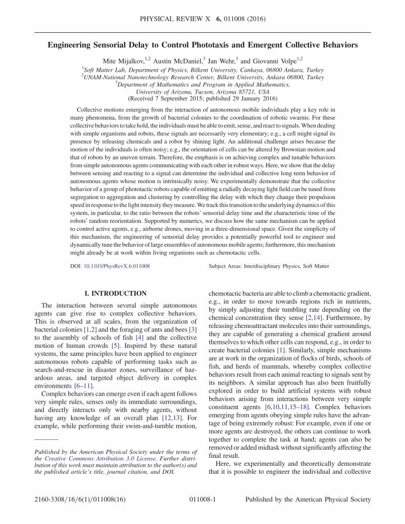
FIG. 1. (a) An autonomous agent, whose position at time t is ðxt; ytÞ, moves with speed v in the direction described by ϕt,corresponding to its instantaneous orientation (arrow), which varies randomly with a characteristic time τ. (b) Picture of a phototacticrobot in a light gradient generated by an infrared lamp. The propulsion speed of the robot depends on the instantaneously measured lightintensity, while its orientation changes randomly. A sample trajectory is shown by the gray solid line. (c) Relation between the measuredlight intensity I and the robot’s speed v [Eq. (3)].

MIJALKOV, MCDANIEL, WEHR, and VOLPE PHYS. REV. X 6, 011008 (2016)

011008-2

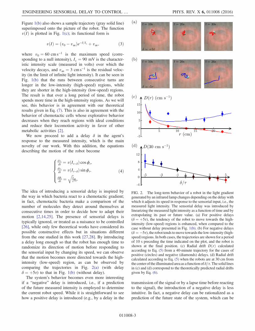
Figure 1(b) also shows a sample trajectory (gray solid line)superimposed onto the picture of the robot. The functionvðIÞ is plotted in Fig. 1(c); its functional form is

vðIÞ ¼ ðv0 − v∞Þe−I=Ic þ v∞; ð3Þ

where v0 ¼ 60 cm s−1 is the maximum speed (corre-sponding to a null intensity), Ic ¼ 90 mV is the character-istic intensity scale (measured in volts) over which thevelocity decays, and v∞ ¼ 3 cm s−1 is the residual veloc-ity (in the limit of infinite light intensity). It can be seen inFig. 1(b) that the runs between consecutive turns arelonger in the low-intensity (high-speed) regions, whilethey are shorter in the high-intensity (low-speed) regions.The result is that over a long period of time, the robotspends more time in the high-intensity regions. As we willsee, this behavior is in agreement with our theoreticalresults given in Eq. (7). This is also in agreement with thebehavior of chemotactic cells whose explorative behaviordecreases when they reach regions with ideal conditionsand reduce their locomotion activity in favor of othermetabolic activities [2].We now proceed to add a delay δ in the agent’s

response to the measured intensity, which is the mainnovelty of our work. With this addition, the equationsdescribing the motion of the robot become

8>>><>>>:

dxtdt ¼ vðIt−δÞ cosϕt;dytdt ¼ vðIt−δÞ sinϕt;

dϕtdt ¼

ffiffi2τ

qηt:

ð4Þ

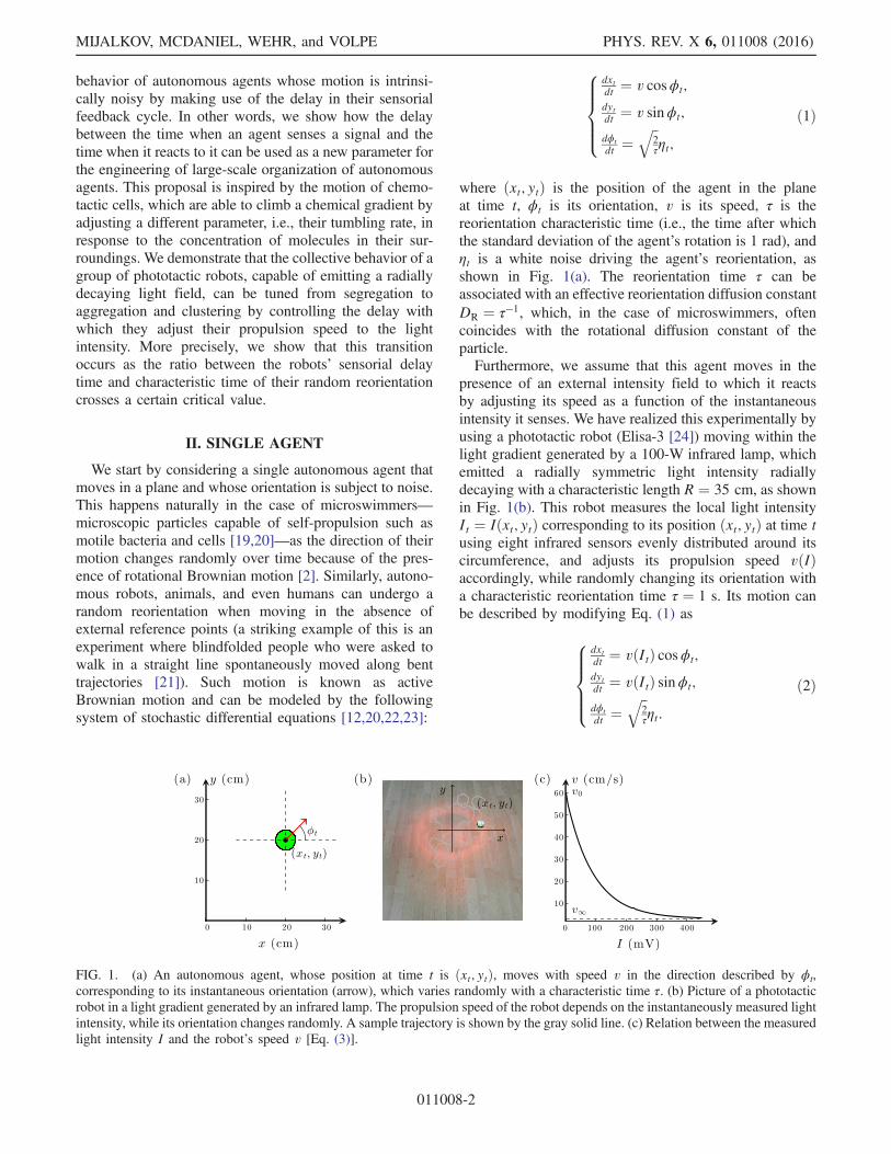
The idea of introducing a sensorial delay is inspired bythe way in which bacteria react to a chemotactic gradient;in fact, chemotactic bacteria make a comparison of thenumber of molecules they detect around themselves atconsecutive times in order to decide how to adapt theirmotion [2,14,25]. The presence of sensorial delays istypically ignored, or treated as a nuisance to be controlled[26], while only few theoretical works have considered itspossible constructive effects but in situations differentfrom the one studied in this work [27,28]. By introducinga delay long enough so that the robot has enough time torandomize its direction of motion before responding tothe sensorial input by changing its speed, we can observethat the motion becomes more directed towards the high-intensity (low-speed) region, as can be observed bycomparing the trajectories in Fig. 2(a) (with delayδ ¼ þ5τ) to that in Fig. 1(b) (without delay).The system’s behavior becomes even more interesting

if a “negative” delay is introduced, i.e., if a predictionof the future measured intensity is employed to determinethe current robot speed. While it is straightforward to seehow a positive delay is introduced (e.g., by a delay in the

transmission of the signal or by a lapse time before reactingto the signal), the introduction of a negative delay is lessintuitive. In fact, a negative delay can be rationalized as aprediction of the future state of the system, which can be

FIG. 2. The long-term behavior of a robot in the light gradientgenerated by an infrared lamp changes depending on the delay withwhich it adjusts its speed in response to the sensorial input, i.e., themeasured light intensity. The sensorial delay was introduced bylinearizing the measured light intensity as a function of time and byextrapolating its past or future value. (a) For positive delays(δ ¼ þ5τ), the tendency of the robot to move towards the high-intensity (low-speed) regions is enhanced, when compared to thecase without delay presented in Fig. 1(b). (b) For negative delays(δ ¼ −5τ), the robot tends tomove towards the low-intensity (high-speed) regions. In both cases, the trajectories are shown for a periodof 10 s preceding the time indicated on the plot, and the robot isshown at the final position. (c) Radial drift DðrÞ calculatedaccording to Eq. (5) from a 40-minute trajectory for the cases ofpositive (circles) and negative (diamonds) delays. (d) Radial driftcalculated according to Eq. (5) when the robots are at 30 cm fromthe center of the illuminated area as a function of δ=τ. The solid linesin (c) and (d) correspond to the theoretically predicted radial driftsgiven by Eq. (6).

ENGINEERING SENSORIAL DELAY TO CONTROL … PHYS. REV. X 6, 011008 (2016)

011008-3

done based on the signal received up to the present time.For example, in the case of our robots, a negative delay isintroduced by linearizing the light intensity measurement asa function of time and extrapolating it into the future, i.e.,Iðt − δÞ ≈ IðtÞ − δI0ðtÞ, where both IðtÞ and I0ðtÞ areknown at time t; higher-order predictor algorithms arealso possible, making use of more information about theevolution of the intensity measured up to the present. Weshow the corresponding trajectory in Fig. 2(b), whereδ ¼ −5τ. In this case, the robot escapes from the high-intensity region and moves towards the edge, where theinfrared lamp intensity is lower (and the speed higher).In order to quantify these observations, we have mea-

sured the effective radial drift of the robots, which iscalculated [29] as

DðrÞ ¼ 1

Δthrnþ1 − rnjrn ≅ ri; ð5Þ

where r is the radial coordinate, rn are samples of therobot’s radial position, and Δt is the time step betweensamples. The results are shown in Figs. 2(c) and 2(d). Forpositive delay (red circles), the negative drift for large radialdistance shows that the robot tends to move towards thecentral high-intensity region. For negative delay (bluediamonds), the positive drift shows that the robot escapesfrom the central high-intensity region. We have alsotheoretically calculated the radial drift for an autonomousagent whose motion is governed by Eq. (4) (the derivation

is outlined in Appendix A and described in detail inAppendix B), obtaining

DðrÞ ¼ τ

2

�1 − δ

τ

�vðrÞ dv

drðrÞ þ τvðrÞ2

r; ð6Þ

where vðrÞ ¼ vðIðrÞÞ and we have assumed a radiallysymmetric intensity distribution. The solid lines plotted inFigs. 2(c) and 2(d) show that there is a good agreementbetween these theoretical predictions and the experimen-tally measured data. We have further corroborated theseresults with numerical simulations, whose results, shown inFig. 3, are in good agreement with the experimental resultsshown in Fig. 2. The numerical simulations were performedby solving the finite difference approximation of Eq. (4)[20,30]. The delayed sensorial measurement was evaluatedby the Taylor expansion of the measured intensity about theagent’s location and extrapolating the corresponding past orfuture value.

FIG. 3. Simulated trajectories for autonomous agents in anintensity field (background yellow shading) for delays(a) δ ¼ þ5τ, (b) δ ¼ 0, and (c) δ ¼ −5τ. The agents are confinedin a circular well (gray border). (d) Radial drift as a function ofthe delay calculated from 1000 simulated trajectories of thesystem evolving for 100 s for the cases of positive (circles) andnegative (diamonds) delays. The solid lines correspond to thetheoretically predicted radial drift given by Eq. (6). Comparingthese results with the ones shown in Fig. 2, we observe a goodagreement between simulation and experiment.

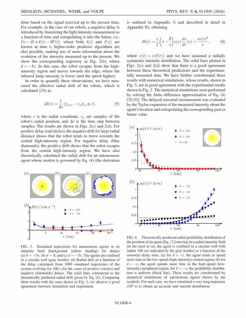
FIG. 4. Theoretically predicted radial probability distribution ofthe position of an agent [Eq. (7)] moving in a radial intensity field[in the inset in (a), the agent is confined in a circular well withradius 100 cm indicated by the gray border] as a function of thesensorial delay time: (a) for δ > −τ, the agent tends to spendmore time in the low-speed (high-intensity) central region; (b) forδ < −τ, the agent spends more time in the high-speed (low-intensity) peripheral region; for δ ¼ −τ, the probability distribu-tion is uniform (black line). These results are corroborated bynumerical simulations of autonomous agents shown by thesymbols. For each case, we have simulated a very long trajectory(108 s) to obtain an accurate and smooth distribution.

MIJALKOV, MCDANIEL, WEHR, and VOLPE PHYS. REV. X 6, 011008 (2016)

011008-4

We can also theoretically derive the approximate steady-state probability distribution of the agent’s position (thederivation is outlined in Appendix A and described in detailin Appendix B), which exists and equals

ρ0ðx; yÞ ¼1

Nvðx; yÞ1þðδ=τÞ ; ð7Þ

provided that the normalization constant

N ¼Z

vðx; yÞ−½1þðδ=τÞ�dxdy < ∞:

Equation (6) confirms our initial observations that thelarger the positive delay is [solid lines in Fig. 4(a)], themore time the agent spends in the low-speed (high-intensity) regions. On the other hand, the more negativethe delay is [solid lines in Fig. 4(b)], the more time theagent spends in the high-speed (low-intensity) regions.Interestingly, we note that there is a cutoff value at δ ¼ −τfor which the probability distribution of the agent isuniform [black solid line in Fig. 4(b)]. We have furthercorroborated these results with numerical simulationsshown by the symbols in Figs. 4(a) and 4(b).We emphasize that the qualitative change of the particle’s

behavior occurs at a negative delay, i.e., δ ¼ −τ.Introduction of negative delays is thus crucial for thedescribed transition. On the other hand, positive delaysalso strongly influence the system’s behavior. While with-out delay the particle spends more time in slow regions, apositive delay makes this tendency more pronounced, asclearly seen at the quantitative level from Eq. (7). Thistendency persists, albeit in a weaker form, for smallnegative delays −τ < δ < 0 and gets reversed at the criticalvalue δ ¼ −τ.

III. MULTIPLE AGENTS

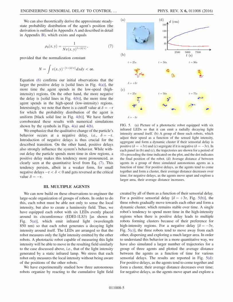
We can now build on these observations to engineer thelarge-scale organization of groups of robots. In order to dothis, each robot must be able not only to sense the localintensity, but also to create a luminosity field. Thus, wehave equipped each robot with six LEDs evenly placedaround its circumference (EDEI-1LS3) [as shown inFig. 5(a)], which emit infrared light (wavelength850 nm) so that each robot generates a decaying lightintensity around itself. The LEDs are arranged so that therobot measures only the light intensity emitted by the otherrobots. A phototactic robot capable of measuring this lightintensity will be able to move in the resulting field similarlyto the case discussed above, i.e., that of the light intensitygenerated by a static infrared lamp. We stress that eachrobot only measures the local intensity without being awareof the positions of the other robots.We have experimentally studied how three autonomous

robots organize by reacting to the cumulative light field

created by all of them as a function of their sensorial delay.For a positive sensorial delay [δ ¼ þ3τ, Fig. 5(b)], thethree robots gradually move towards each other and form adynamic cluster, which remains stable over time. A singlerobot’s tendency to spend more time in the high-intensityregions when there is positive delay leads to multiplerobots forming clusters because of their preference forhigh-intensity regions. For a negative delay [δ ¼ −3τ,Fig. 5(c)], the three robots tend to move away from eachother, dispersing and exploring a much larger area. In orderto understand this behavior in a more quantitative way, wehave also simulated a larger number of trajectories for agroup of three agents and plotted the average distancebetween the agents as a function of time for varioussensorial delays. The results are reported in Fig. 5(d):For positive delays, as the agents tend to come together andform a cluster, their average distance decreases over time;for negative delays, as the agents move apart and explore a

FIG. 5. (a) Picture of a phototactic robot equipped with sixinfrared LEDs so that it can emit a radially decaying lightintensity around itself. (b) A group of three such robots, whichadjust their speed as a function of the sensed light intensity,aggregate and form a dynamic cluster if their sensorial delay ispositive (δ ¼ þ3τ) and (c) segregate if it is negative (δ ¼ −3τ). Ineach panel in (b) and (c), the trajectories are shown for a period of10 s preceding the time indicated on the plot, and the dot indicatesthe final position of the robot. (d) Average distance d betweenagents in a group of three simulated autonomous agents as afunction of time: For positive delays, as the agents tend to cometogether and form a cluster, their average distance decreases overtime; for negative delays, as the agents move apart and explore alarger area, their average distance increases.

ENGINEERING SENSORIAL DELAY TO CONTROL … PHYS. REV. X 6, 011008 (2016)

011008-5

larger area, their average distance increases. The qualitativechange of the agents’ behavior occurs at a strictly negativevalue of the dimensionless parameter δ=τ ¼ −1 [seeEq. (7)]. While introduction of negative delays is thuscrucial for the described transition from aggregation tosegregation, positive delays also strongly influence thesystem’s behavior by enhancing the tendency of the agentsto aggregate. Importantly, not only a light field, but anyradially decaying scalar (e.g., chemical, acoustic) fieldcreated by the autonomous agents can be used in orderto achieve this kind of control over their behavior.In order to explore the scalability of this mechanism, we

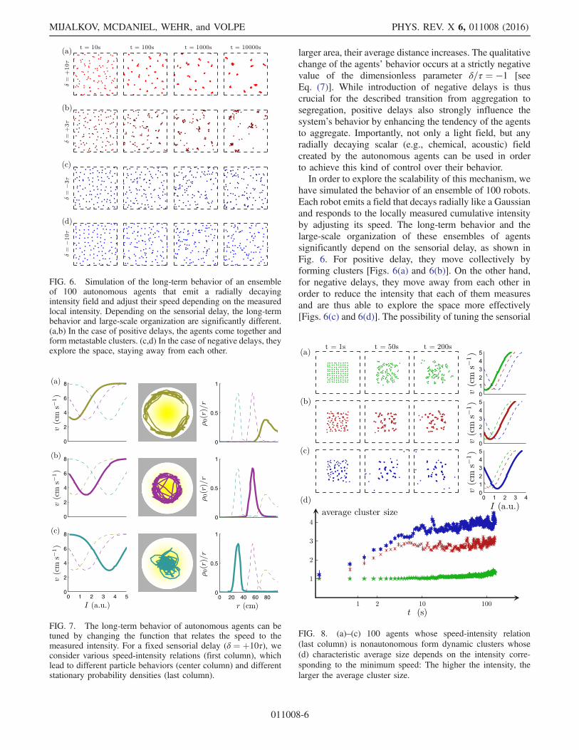
have simulated the behavior of an ensemble of 100 robots.Each robot emits a field that decays radially like a Gaussianand responds to the locally measured cumulative intensityby adjusting its speed. The long-term behavior and thelarge-scale organization of these ensembles of agentssignificantly depend on the sensorial delay, as shown inFig. 6. For positive delay, they move collectively byforming clusters [Figs. 6(a) and 6(b)]. On the other hand,for negative delays, they move away from each other inorder to reduce the intensity that each of them measuresand are thus able to explore the space more effectively[Figs. 6(c) and 6(d)]. The possibility of tuning the sensorial

0 1 2 3 4 50

2

4

6

8

0

2

4

6

8

0

2

4

6

8

0 20 40 60 800

0.5

1

0

0.5

1

0

0.5

1

FIG. 7. The long-term behavior of autonomous agents can betuned by changing the function that relates the speed to themeasured intensity. For a fixed sensorial delay (δ ¼ þ10τ), weconsider various speed-intensity relations (first column), whichlead to different particle behaviors (center column) and differentstationary probability densities (last column).

FIG. 8. (a)–(c) 100 agents whose speed-intensity relation(last column) is nonautonomous form dynamic clusters whose(d) characteristic average size depends on the intensity corre-sponding to the minimum speed: The higher the intensity, thelarger the average cluster size.

FIG. 6. Simulation of the long-term behavior of an ensembleof 100 autonomous agents that emit a radially decayingintensity field and adjust their speed depending on the measuredlocal intensity. Depending on the sensorial delay, the long-termbehavior and large-scale organization are significantly different.(a,b) In the case of positive delays, the agents come together andform metastable clusters. (c,d) In the case of negative delays, theyexplore the space, staying away from each other.

MIJALKOV, MCDANIEL, WEHR, and VOLPE PHYS. REV. X 6, 011008 (2016)

011008-6

delay can be exploited, for example, in a search-and-rescuetask by initially setting a negative delay so that the robotscan thoroughly explore the environment and, at a laterstage, a positive delay so that the robots can be collectedinto clusters to share the gathered information. Collectingall robots can also be easily achieved by sending a strongsignal capable of eclipsing the signals emitted by the robotsthemselves.It is also possible to adjust the behavior of the agents by

altering the intensity-speed relation to something differentthan Eq. (3). For example, instead of a monotonicallydecreasing relation, it is possible to use a relation with aminimum at some specific value. As can be seen in Fig. 7,this alters the agent’s behavior so that it spends more timewhere the intensity corresponds to the minimum speed. Inthis way, it is possible to control where the agent will spendmost of its time, which may be useful, e.g., for targeteddelivery. Furthermore, in the presence of multiple agentscapable of emitting a radially decaying intensity field,changing the intensity-speed relation permits one to controlvarious features of the clusters such as their characteristicsize, as shown in Fig. 8.

IV. SINGLE AND MULTIPLE ROBOTSIN THREE DIMENSIONS

Our results can also be extended to the three-dimensionalcase, where they still hold with only minor adjustments.This could be important when considering airborne objects(e.g., drones, flying insects, birds) or underwater objects(e.g., fish, submarine robots). In three dimensions, theautonomous agent motion can be modeled by the set ofequations

8>>>>>>>>><>>>>>>>>>:

dxtdt ¼ vðIt−δÞ sin θt cosϕt;dytdt ¼ vðIt−δÞ sin θt sinϕt;dztdt ¼ vðIt−δÞ cos θt;dθtdt ¼ 1

τ cot θt þffiffi2τ

qηð1Þt ;

dϕtdt ¼ 1

sin θt

ffiffi2τ

qηð2Þt ;

ð8Þ

where ðxt; yt; ztÞ is the position of the agent at time t, θt andϕt are its azimuthal and polar orientations, respectively, and

ηð1Þt and ηð2Þt are independent white noises. Similar equa-tions but without delay have already been considered, e.g.,in Ref. [31], to describe active Brownian motion in threedimensions. The last two equations describe (accelerated)Brownian motion on the surface of the unit sphere.From this model, we obtain the approximate steady-stateprobability distribution (the derivation is described inAppendix B), which exists and equals

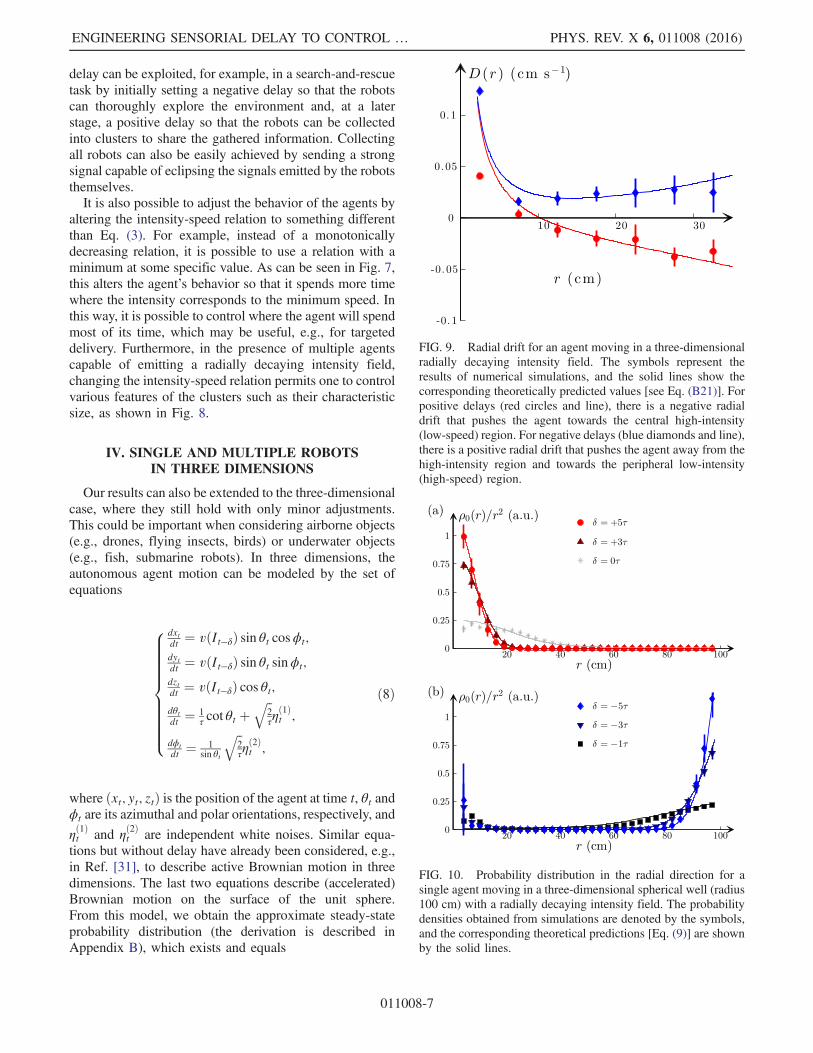
FIG. 9. Radial drift for an agent moving in a three-dimensionalradially decaying intensity field. The symbols represent theresults of numerical simulations, and the solid lines show thecorresponding theoretically predicted values [see Eq. (B21)]. Forpositive delays (red circles and line), there is a negative radialdrift that pushes the agent towards the central high-intensity(low-speed) region. For negative delays (blue diamonds and line),there is a positive radial drift that pushes the agent away from thehigh-intensity region and towards the peripheral low-intensity(high-speed) region.

FIG. 10. Probability distribution in the radial direction for asingle agent moving in a three-dimensional spherical well (radius100 cm) with a radially decaying intensity field. The probabilitydensities obtained from simulations are denoted by the symbols,and the corresponding theoretical predictions [Eq. (9)] are shownby the solid lines.

ENGINEERING SENSORIAL DELAY TO CONTROL … PHYS. REV. X 6, 011008 (2016)

011008-7

ρ0ðx; y; zÞ ¼1

Mvðx; y; zÞ1þ2ðδ=τÞ ; ð9Þ

provided that the normalization constant

M ¼Z

vðx; y; zÞ−½1þ2ðδ=τÞ�dxdydz < ∞:

Comparing Eq. (9) and Eq. (7), we note that the maindifference is that in the three-dimensional case, the uniformdistribution occurs for δ ¼ −0.5τ instead of for δ ¼ −τ.Otherwise, the agents still exhibit a qualitatively differentbehavior for positive and negative sensorial delay, corre-sponding, respectively, to an effective drift towards high-intensity and low-intensity regions, as illustrated in Figs. 9and 10. As in the two-dimensional case, in the three-dimensional case, it is also possible to engineer this drift bychanging the time delay in order to tune the collectivebehavior of a swarm from aggregation and clustering tosegregation.

V. CONCLUSION

We have demonstrated the use of delayed sensorial feed-back to control the organization of an ensemble of autono-mous agents.We realized this model experimentally by usingautonomous robots, further backed it upwith simulations, andfinally provided a mathematical analysis that agrees with theresults obtained in the experiments and simulations. Ourfindings show that a single robot, measuring the intensitylocally, spends more time in either a high- or a low-intensityregion depending on its sensorial delay. Tuning the value ofthe delay permits one to engineer the behavior of an ensembleof robots so that they come together or separate from eachother. The robustness and flexibility of these behaviors arevery promising for applications in the field of swarm robotics[6,10,11,16,18], as well as in the assembly of nanorobots,e.g., for targeted delivery within tissues. Furthermore, sincesome living entities, such as bacteria, are known to respond totemporal evolution of stimuli [2,25], the presence of asensorial delay could also explain the swarming behaviorof groups of living organisms.

ACKNOWLEDGMENTS

The authors thank Gilles Caprari (GCtronic) for hishelp with the robots. G. V. thanks Holger Stark for usefuldiscussions that led to the original idea for this work.J. W. and A.M. were partially supported by the NSF GrantsNo. DMS 1009508 and No. DMS 0623941. The work ofJ. W. was partially supported by NSF under GrantNo. DMS 1440140 while he was in residence at theMathematical Sciences Research Institute in Berkeleyduring 2015. G. V. was partially supported by MarieCurie Career Integration Grant (MC-CIG) No. PCIG11GA-2012-321726 and the Turkish Academy of Sciences

(TÜBA). M.M. was partially supported by Tubitak GrantNo. 113Z556.

APPENDIX A: MATHEMATICALDERIVATION—AN OUTLINE

We studied the limit of the system (4) as δ, τ → 0 at thesame rate so that δ ¼ cϵ and τ ¼ kϵ, where c and k remainconstant in the limit δ, τ, ϵ → 0. We expanded v about t tofirst order in δ and solved the resulting equations for _x and_y. We expanded the resulting system to first order in thesmall parameter δ=

ffiffiffiτ

p. We then considered the correspond-

ing backward Kolmogorov equation for the probabilitydensity ρ. We expanded ρ in powers of the parameter

ffiffiffiϵ

p,

i.e., ρ ¼ ρ0 þffiffiffiϵ

pρ1 þ ϵρ2 þ � � �, and used the standard

multiscale expansion method [32] to derive the backwardKolmogorov equation for the limiting density ρ0:

∂ρ0∂t ¼ τ

2

�1−δ

τ

�v

�∂v∂x

∂ρ0∂x þ∂v

∂y∂ρ0∂y

�þτv2

2Δρ0: ðA1Þ

From this equation, we got the limiting SDE:

8<:

dxt ¼ τ2

�1 − δ

τ

�vðxt; ytÞ ∂v∂x ðxt; ytÞdtþ

ffiffiffiτ

pvðxt; ytÞdW1

t ;

dyt ¼ τ2

�1 − δ

τ

�vðxt; ytÞ ∂v∂y ðxt; ytÞdtþ

ffiffiffiτ

pvðxt; ytÞdW2

t ;

ðA2Þ

where W1 and W2 are independent Wiener processes.Assuming that v is rotationally invariant, from Eq. (A2),we obtain the formula for the radial drift [Eq. (6)]:

DðrÞ ¼ τ

2

�1 − δ

τ

�vðrÞ dv

drðrÞ þ τvðrÞ2

r: ðA3Þ

Setting the right-hand side of the forward (Fokker-Planck)equation corresponding to Eq. (A1) equal to zero, we getthe formula for the stationary probability density ρ0 (if itexists) [Eq. (7)],

ρ0ðx; yÞ ¼1

Nvðx; yÞ1þðδ=τÞ ; ðA4Þ

where N is the normalization constant. A similar analysisfollows for the three-dimensional case, leading to the three-dimensional stationary probability density given by Eq. (9).A more detailed derivation is provided in the followingappendix.

APPENDIX B: MATHEMATICALDERIVATION—DETAILS

1. Mathematical derivation in two dimensions

Our motivation is the system given by Eq. (4), which wecan rewrite as

MIJALKOV, MCDANIEL, WEHR, and VOLPE PHYS. REV. X 6, 011008 (2016)

011008-8

8>>><>>>:

dxtdt ¼ vðxt−δ; yt−δÞ cosϕt;dytdt ¼ vðxt−δ; yt−δÞ sinϕt;

dϕtdt ¼

ffiffi2τ

qηt:

While the reorientation characteristic time τ is constantin the experiment, to analyze the system mathematicallywe study the limit as τ and δ go to zero. Thus, in themathematical analysis, we use ~τ and ~δ to represent thereorientation characteristic time and time delay, in order todifferentiate these parameters that will go to zero from thereorientation characteristic time τ and time delay δ in theexperiment. If τ is very small, a particle that movesaccording to the above equations changes direction veryrapidly; thus, for the displacement of this particle from itsinitial position to be significant, the particle must have alarge speed. We account for this mathematically by letting vincrease as ~τ decreases. In order to obtain nontrivialbehavior in the limit, we must define v ¼ ðu= ffiffiffi

~τp Þ, where

u does not depend on ~τ. Then, we have

8>>><>>>:

dxt ¼ 1ffiffi~τ

p uðxt−~δ; yt−~δÞ cosϕtdt;

dyt ¼ 1ffiffi~τ

p uðxt−~δ; yt−~δÞ sinϕtdt;

dϕt ¼ffiffi2~τ

qdWt;

where Wt is a Wiener process.We expand u about t to first order in ~δ. The resulting

system approximates the above equations and is also thesystem actually used in numerical simulation. We thusstudy the approximate equations:

8>>>>><>>>>>:

_xt¼ 1ffiffi~τ

phuðxt;ytÞ− ~δ∂u∂xðxt;ytÞ_xt− ~δ∂u∂yðxt;ytÞ_yt

icosϕt;

_yt¼ 1ffiffi~τ

phuðxt;ytÞ− ~δ∂u∂xðxt;ytÞ_xt− ~δ∂u∂yðxt;ytÞ_yt

isinϕt;

ϕt¼ffiffi2~τ

qWt:

Solving the first two equations for _xt and _yt, we get

8>>>>><>>>>>:

_xt ¼ 1ffiffi~τ

p uðxt; ytÞ cosϕt ×h1þ ~δffiffi

~τp

�∂u∂x ðxt; ytÞ cosϕt þ ∂u

∂y ðxt; ytÞ sinϕt

�i−1;

_yt ¼ 1ffiffi~τ

p uðxt; ytÞ sinϕt ×h1þ ~δffiffi

~τp

�∂u∂x ðxt; ytÞ cosϕt þ ∂u

∂y ðxt; ytÞ sinϕt

�i−1;

ϕt ¼ffiffi2~τ

qWt:

We approximate the system further, for ð~δ= ffiffiffi~τ

p Þ ≪ 1, by

8>>>>><>>>>>:

dxt ¼ 1ffiffi~τ

p uðxt; ytÞ cosϕt ×h1 − ~δffiffi

~τp

�∂u∂x ðxt; ytÞ cosϕt þ ∂u

∂y ðxt; ytÞ sinϕt

�idt;

dyt ¼ 1ffiffi~τ

p uðxt; ytÞ sinϕt ×h1 − ~δffiffi

~τp

�∂u∂x ðxt; ytÞ cosϕt þ ∂u

∂y ðxt; ytÞ sinϕt

�idt;

dϕt ¼ffiffi2~τ

qdWt:

ðB1Þ

We study the limit of the system (B1) as ~δ and ~τ go to zero at the same rate. This is consistent with the assumptionð~δ= ffiffiffi

~τp Þ ≪ 1. Thus, we suppose that ~δ and ~τ stay proportional to a single characteristic time ϵ, i.e., ~δ ¼ cϵ and ~τ ¼ kϵ, where

c and k remain constant in the limit ~δ, ~τ, ϵ → 0. Writing Eq. (B1) in terms of ϵ, we obtain

8>>>>><>>>>>:

dxt ¼�

1ffiffiffiffikϵ

p u cosϕt − ck u

∂u∂x cos2ϕt − c

k u∂u∂y cosϕt sinϕt

�dt;

dyt ¼�

1ffiffiffiffikϵ

p u sinϕt − ck u

∂u∂x cosϕt sinϕt − c

k u∂u∂y sin2ϕt

�dt;

dϕt ¼ffiffiffiffi2kϵ

qdWt:

ðB2Þ

We take the limit ϵ → 0 by using the multiscale expansion method (a detailed exposition can be found in, e.g., Ref. [32]).The backward Kolmogorov equation corresponding to the system (B2) of SDEs is

ENGINEERING SENSORIAL DELAY TO CONTROL … PHYS. REV. X 6, 011008 (2016)

011008-9

∂ρ∂t ¼

1

kϵ∂2ρ

∂ϕ2þ 1ffiffiffiffiffi

kϵp u cosϕ

∂ρ∂xþ

1ffiffiffiffiffikϵ

p u sinϕ∂ρ∂y

−�cku∂u∂x cos

2 ϕþ cku∂u∂y cosϕ sinϕ

� ∂ρ∂x

−�cku∂u∂x cosϕ sinϕþ c

ku∂u∂y sin

2 ϕ

� ∂ρ∂y ;

which can be written as

∂ρ∂t ¼

�1

ϵL0 þ

1ffiffiffiϵ

p L1 þ L2

�ρ; ðB3Þ

where

L0 ¼1

k∂2

∂ϕ2;

L1 ¼1ffiffiffik

p u cosϕ∂∂xþ

1ffiffiffik

p u sinϕ∂∂y ;

and

L2 ¼ −�cku∂u∂x cos

2ϕþ cku∂u∂y cosϕ sinϕ

� ∂∂x

−�cku∂u∂x cosϕ sinϕþ c

ku∂u∂y sin

2ϕ

� ∂∂y :

We expand ρ in powers offfiffiffiϵ

p,

ρ ¼ ρ0 þffiffiffiϵ

pρ1 þ ϵρ2 þ � � � ; ðB4Þ

and derive the backward Kolmogorov equation for thelimiting density ρ0. First, substituting Eq. (B4) in Eq. (B3)and equating terms of the same order in

ffiffiffiϵ

pgives the

equations

O

�1

ϵ

�∶ L0ρ0 ¼

1

k∂2ρ0∂ϕ2

¼ 0; ðB5Þ

O

�1ffiffiffiϵ

p�∶L1ρ0þL0ρ1

¼ 1ffiffiffik

p ucosϕ∂ρ0∂x þ 1ffiffiffi

kp usinϕ

∂ρ0∂y þ1

k∂2ρ1∂ϕ2

¼0;

ðB6Þ

Oð1Þ∶ L2ρ0 þ L1ρ1 þ L0ρ2 ¼∂ρ0∂t : ðB7Þ

While fðx; y;ϕ; tÞ ¼ Aðx; y; tÞϕþ Bðx; y; tÞ is the generalsolution to Eq. (B5), we expect ρ0 to be independent of ϕ,and therefore, we choose ρ0 ¼ ρ0ðx; y; tÞ. Next, we find ρ1in terms of ρ0 by solving Eq. (B6); since ρ0 does not dependon ϕ, we have

ρ1 ¼ffiffiffik

pu∂ρ0∂x cosϕþ

ffiffiffik

pu∂ρ0∂y sinϕ;

where we leave out a linear term in ϕ in order to make ρ1periodic in ϕ. We could include a term that is constant in ϕ,but this would not change the final result. Equation (B7)implies that the function ð∂ρ0=∂tÞ − L1ρ1 − L2ρ0 is in therange of the operator L0. This is a self-adjoint operator onthe space L2½0; 2π�, so the above function must beorthogonal to its kernel, which, in particular, containsconstants. It follows that

1

2π

Z2π

0

�∂ρ0∂t − L1ρ1 − L2ρ0

�dϕ ¼ 0

so that

∂ρ0∂t ¼ 1

2π

Z2π

0

��1ffiffiffik

p u cosϕ∂∂xþ

1ffiffiffik

p u sinϕ∂∂y

�

×

� ffiffiffik

pu∂ρ0∂x cosϕþ

ffiffiffik

pu∂ρ0∂y sinϕ

�

−�cku∂u∂x cos

2ϕþ cku∂u∂y cosϕ sinϕ

� ∂ρ0∂x

−�cku∂u∂x cosϕ sinϕþ c

ku∂u∂y sin

2ϕ

� ∂ρ0∂y

�dϕ;

and so

∂ρ0∂t ¼ u

2

∂∂x

�u∂ρ0∂x

�þ u

2

∂∂y

�u∂ρ0∂y

�− c2k

u∂u∂x

∂ρ0∂x

− c2k

u∂u∂y

∂ρ0∂y

or, equivalently,

∂ρ0∂t ¼

�1 − c

k

2

�u

�∂u∂x

∂ρ0∂x þ ∂u

∂y∂ρ0∂y

�þ u2

2Δρ0:

In order to compare this with the experimental results, wesubstitute u ¼ ffiffiffi

τp

v, where τ is the reorientation character-istic time in the experiments, to obtain

∂ρ0∂t ¼ τ

2

�1− δ

τ

�v

�∂v∂x

∂ρ0∂x þ ∂v

∂y∂ρ0∂y

�þ τv2

2Δρ0: ðB8Þ

a. Radial drift [Eq. (6)]

Equation (B8) is the backward Kolmogorov equation forthe SDE system

MIJALKOV, MCDANIEL, WEHR, and VOLPE PHYS. REV. X 6, 011008 (2016)

011008-10

8<:

dxt ¼ τ2

�1 − δ

τ

�vðxt; ytÞ ∂v∂x ðxt; ytÞdtþ

ffiffiffiτ

pvðxt; ytÞdW1

t ;

dyt ¼ τ2

�1 − δ

τ

�vðxt; ytÞ ∂v∂y ðxt; ytÞdtþ

ffiffiffiτ

pvðxt; ytÞdW2

t ;

where W1 and W2 are independent Wiener processes.Letting r ¼

ffiffiffiffiffiffiffiffiffiffiffiffiffiffiffix2 þ y2

pand applying the Itô formula, we

obtain

drt ¼�τ

2

�1 − δ

τ

�v

�∂v∂x

∂r∂xþ

∂v∂y

∂r∂y

�

þ τv2

2

�∂2r∂x2 þ

∂2r∂y2

��dt

þ ffiffiffiτ

pv

�∂r∂x dW

1t þ

∂r∂y dW

2t

�

or, equivalently,

drt ¼�τ

2

�1 − δ

τ

�vrt

�xt∂v∂x þ yt

∂v∂y

�þ τv2

rt

�dt

þffiffiffiτ

pv

rtðxtdW1

t þ ytdW2t Þ:

Assuming v is radially symmetric, i.e., vðx; yÞ ¼ vðrÞ withr ¼

ffiffiffiffiffiffiffiffiffiffiffiffiffiffiffix2 þ y2

p, we have

drt ¼�τ

2

�1 − δ

τ

�vðrtÞ

dvdr

ðrtÞ þτvðrtÞ2

rt

�dt

þffiffiffiτ

pvðrtÞrt

ðxtdW1t þ ytdW2

t Þ: ðB9Þ

We note that ðxt=rtÞdW1t þ ðyt=rtÞdW2

t is the stochasticdifferential of the martingale

Bt ¼Z

t

0

�xsrsdW1

s þysrsdW2

s

�;

which is a Wiener process by the Lévy theorem [33][Theorem 8.6.1] because its quadratic variation is equal tot. Thus, the effective radial drift is given by

DðrÞ ¼ τ

2

�1 − δ

τ

�vðrÞ dv

drðrÞ þ τvðrÞ2

r: ðB10Þ

b. Density [Eq. (7)]

The forward Kolmogorov equation corresponding toEq. (B8) is

∂ρ0∂t ¼ − τ

2

�1 − δ

τ

�� ∂∂x

�v∂v∂x ρ0

�þ ∂∂y

�v∂v∂y ρ0

��

þ τ

2Δðv2ρ0Þ:

Thus, the stationary probability density ρ0 satisfies

− τ

2

�1 − δ

τ

�� ∂∂x

�v∂∂x ρ0

�þ ∂∂y

�v∂∂y ρ0

��

þ τ

2Δðv2ρ0Þ ¼ 0: ðB11Þ

One can check that

ρ0ðx; yÞ ¼1

Nvðx; yÞ1þðδ=τÞ ; ðB12Þ

whereN is the normalization constant, is a positive solutionof Eq. (B11).

2. Mathematical derivation in three dimensions

Equation (8) describes the motion of a particle in threedimensions whose speed is given by vðx; y; zÞ and whosedirection is given by an accelerated Wiener process on thesurface of the unit sphere (just like in two dimensions,

eiffiffiffiffiffiffiffiffið2=τÞ

pWt is an accelerated Wiener process on the unit

circle). The precise form of the equations is8>>>>>>>>>>><>>>>>>>>>>>:

dxt ¼ 1ffiffi~τ

p uðxt−~δ; yt−~δ; zt−~δÞ sin θt cosϕtdt;

dyt ¼ 1ffiffi~τ

p uðxt−~δ; yt−~δ; zt−~δÞ sin θt sinϕtdt;

dzt ¼ 1ffiffi~τ

p uðxt−~δ; yt−~δ; zt−~δÞ cos θtdt;

dθt ¼ 1~τ cot θtdtþ

ffiffi2~τ

qdW1

t ;

dϕt ¼ffiffi2~τ

q1

sin θtdW2

t :

ðB13Þ

The justification of the last two equations is the following.We start from a Wiener process on the sphere, i.e.,

(d~θt ¼ 1

2cot ~θtdtþ d ~W1

t ;

d ~ϕt ¼ 1

sin ~θtd ~W2

t ;

and rescale the time so that

θt ¼ ~θ2t=~τ;

ϕt ¼ ~ϕ2t=~τ:

It is easy to show that these rescaled processes satisfy thelast two equations of the above system with the newWienerprocesses

Wjt ¼

ffiffiffi~τ

2

r~Wj2t=~τ; j ¼ 1; 2:

We follow the procedure that was used to analyze the two-dimensional case. Let xt ¼ ðxt; yt; ztÞ. In Eq. (B13), weexpand u about t to first order in ~δ to get

ENGINEERING SENSORIAL DELAY TO CONTROL … PHYS. REV. X 6, 011008 (2016)

011008-11

8>>>>>>>>>>>><>>>>>>>>>>>>:

_xt ¼ 1ffiffi~τ

phuðxtÞ − ~δ ∂u

∂x ðxtÞ_xt − ~δ ∂u∂y ðxtÞ_yt − ~δ ∂u

∂z ðxtÞ_ztisin θt cosϕt;

_yt ¼ 1ffiffi~τ

phuðxtÞ − ~δ ∂u

∂x ðxtÞ_xt − ~δ ∂u∂y ðxtÞ_yt − ~δ ∂u

∂z ðxtÞ_ztisin θt sinϕt;

_zt ¼ 1ffiffi~τ

phuðxtÞ − ~δ ∂u

∂x ðxtÞ_xt − ~δ ∂u∂y ðxtÞ_yt − ~δ ∂u

∂z ðxtÞ_zticos θt;

dθt ¼ 1~τ cot θtdtþ

ffiffi2~τ

qdW1

t ;

dϕt ¼ffiffi2~τ

q1

sin θtdW2

t :

ðB14Þ

Solving the first three equations for _xt, _yt, and _zt, we have

8>>>>><>>>>>:

_xt ¼ 1ffiffi~τ

p uðxtÞ cosϕt sin θt ×h1þ ~δffiffi

~τp

�∂u∂x ðxtÞ cosϕt sin θt þ ∂u

∂y ðxtÞ sinϕt sin θt þ ∂u∂z ðxtÞ cos θt

�i−1;

_yt ¼ 1ffiffi~τ

p uðxtÞ sinϕt sin θt ×h1þ ~δffiffi

~τp

�∂u∂x ðxtÞ cosϕt sin θt þ ∂u

∂y ðxtÞ sinϕt sin θt þ ∂u∂z ðxtÞ cos θt

�i−1;

_zt ¼ 1ffiffi~τ

p uðxtÞ cos θt ×h1þ ~δffiffi

~τp

�∂u∂x ðxtÞ cosϕt sin θt þ ∂u

∂y ðxtÞ sinϕt sin θt þ ∂u∂z ðxtÞ cos θt

�i−1:

We approximate the system further, for ð~δ= ffiffiffi~τ

p Þ ≪ 1, by

8>>>>><>>>>>:

dxt ¼ 1ffiffi~τ

p uðxtÞ cosϕt sin θt ×h1 − ~δffiffi

~τp

�∂u∂x ðxtÞ cosϕt sin θt þ ∂u

∂y ðxtÞ sinϕt sin θt þ ∂u∂z ðxtÞ cos θt

�idt;

dyt ¼ 1ffiffi~τ

p uðxtÞ sinϕt sin θt ×h1 − ~δffiffi

~τp

�∂u∂x ðxtÞ cosϕt sin θt þ ∂u

∂y ðxtÞ sinϕt sin θt þ ∂u∂z ðxtÞ cos θt

�idt;

dzt ¼ 1ffiffi~τ

p uðxtÞ cos θt ×h1 − ~δffiffi

~τp

�∂u∂x ðxtÞ cosϕt sin θt þ ∂u

∂y ðxtÞ sinϕt sin θt þ ∂u∂z ðxtÞ cos θt

�idt:

Let ~δ ¼ cϵ, ~τ ¼ kϵ. Then, the system we study is

8>>>>>>>>>>>><>>>>>>>>>>>>:

dxt ¼�

1ffiffiffiffikϵ

p u cosϕt sin θt − ck u

∂u∂x cos2ϕtsin2θt − c

k u∂u∂y cosϕt sinϕtsin2θt − c

k u∂u∂z cosϕt sin θt cos θt

�dt;

dyt ¼�

1ffiffiffiffikϵ

p u sinϕt sin θt − ck u

∂u∂x sinϕt cosϕtsin2θt − c

k u∂u∂y sin2ϕtsin2θt − c

k u∂u∂z sinϕt sin θt cos θt

�dt;

dzt ¼�

1ffiffiffiffikϵ

p u cos θt − ck u

∂u∂x cosϕt sin θt cos θt − c

k u∂u∂y sinϕt sin θt cos θt − c

k u∂u∂z cos2θt

�dt;

dθt ¼ 1kϵ cot θtdtþ

ffiffiffiffi2kϵ

qdW1

t ;

dϕt ¼ffiffiffiffi2kϵ

q1

sin θtdW2

t :

The backward Kolmogorov equation corresponding to the above system of SDEs is

∂ρ∂t ¼

1

kϵ∂2ρ

∂θ2 þ1

kϵ sin2 θ∂2ρ

∂ϕ2þ 1

kϵcot θ

∂ρ∂θ þ

1ffiffiffiffiffikϵ

p u cosϕ sin θ∂ρ∂x

þ 1ffiffiffiffiffikϵ

p u sinϕ sin θ∂ρ∂yþ

1ffiffiffiffiffikϵ

p u cos θ∂ρ∂z

−cku

�∂u∂x cos

2 ϕ sin2 θ þ ∂u∂y cosϕ sinϕ sin2 θ þ ∂u

∂z cosϕ sin θ cos θ

� ∂ρ∂x

−cku

�∂u∂x sinϕ cosϕ sin2 θ þ ∂u

∂y sin2 ϕ sin2 θ þ ∂u

∂z sinϕ sin θ cos θ

� ∂ρ∂y

−cku

�∂u∂x cosϕ sin θ cos θ þ ∂u

∂y sinϕ sin θ cos θ þ ∂u∂z cos

2 θ

� ∂ρ∂z

MIJALKOV, MCDANIEL, WEHR, and VOLPE PHYS. REV. X 6, 011008 (2016)

011008-12

or, equivalently,

∂ρ∂t ¼

�1

ϵL0 þ

1ffiffiffiϵ

p L1 þ L2

�ρ; ðB15Þ

where

L0 ¼1

k

� ∂2

∂θ2 þ1

sin2θ∂2

∂ϕ2þ cot θ

∂∂θ

�; L1 ¼

uffiffiffik

p�cosϕ sin θ

∂∂xþ sinϕ sin θ

∂∂yþ cos θ

∂∂z

�;

and

L2 ¼ − cku

��∂u∂x cos

2ϕsin2θ þ ∂u∂y cosϕ sinϕsin2θ þ ∂u

∂z cosϕ sin θ cos θ

� ∂∂x

þ�∂u∂x sinϕ cosϕsin2θ þ ∂u

∂y sin2ϕsin2θ þ ∂u

∂z sinϕ sin θ cos θ

� ∂∂y

þ�∂u∂x cosϕ sin θ cos θ þ ∂u

∂y sinϕ sin θ cos θ þ ∂u∂z cos

2θ

� ∂∂z

�:

We expand ρ in powers offfiffiffiϵ

p,

ρ ¼ ρ0 þffiffiffiϵ

pρ1 þ ϵρ2 þ � � � : ðB16Þ

Using Eq. (B16) in Eq. (B15) and equating terms of like powers offfiffiffiϵ

pgives the equations

O

�1

ϵ

�∶ L0ρ0 ¼

1

k

�∂2ρ0∂θ2 þ 1

sin2θ∂2ρ0∂ϕ2

þ cot θ∂ρ0∂θ

�¼ 0; ðB17Þ

O

�1ffiffiffiϵ

p�∶ L1ρ0 þ L0ρ1 ¼

uffiffiffik

p cosϕ sin θ∂ρ0∂x þ uffiffiffi

kp sinϕ sin θ

∂ρ0∂y þ uffiffiffi

kp cos θ

∂ρ0∂z

þ 1

k∂2ρ1∂θ2 þ 1

ksin2θ∂2ρ1∂ϕ2

þ 1

kcot θ

∂ρ1∂θ ¼ 0; ðB18Þ

Oð1Þ∶ L2ρ0 þ L1ρ1 þ L0ρ2 ¼∂ρ0∂t : ðB19Þ

In order to satisfy Eq. (B17), we choose ρ0 ¼ ρ0ðx; y; z; tÞ,where we leave out a term of the form Aðx; y; z; tÞϕ becausewe expect ρ0 to be independent of ϕ. Next, we find ρ1 interms of ρ0 by solving Eq. (B18). We see that ρ1 is the sumof the solutions to the partial differential equations (PDEs):

uffiffiffik

p cosϕsinθ∂ρ0∂x þ1

k∂2ρ1∂θ2 þ

1

ksin2θ∂2ρ1∂ϕ2

þ1

kcotθ

∂ρ1∂θ ¼0;

uffiffiffik

p sinϕsinθ∂ρ0∂y þ1

k∂2ρ1∂θ2 þ

1

ksin2θ∂2ρ1∂ϕ2

þ1

kcotθ

∂ρ1∂θ ¼0;

and

uffiffiffik

p cos θ∂ρ0∂z þ 1

k∂2ρ1∂θ2 þ 1

kcot θ

∂ρ1∂θ ¼ 0

or, equivalently,

uffiffiffik

p cosϕsin3θ∂ρ0∂x þ 1

ksin2θ

∂2ρ1∂θ2

þ 1

k∂2ρ1∂ϕ2

þ 1

ksin θ cos θ

∂ρ1∂θ ¼ 0;

uffiffiffik

p sinϕsin3θ∂ρ0∂y þ 1

ksin2θ

∂2ρ1∂θ2 þ 1

k∂2ρ1∂ϕ2

þ 1

ksin θ cos θ

∂ρ1∂θ ¼ 0;

and

1

k∂2ρ1∂θ2 þ 1

kcot θ

∂ρ1∂θ ¼ − uffiffiffi

kp cos θ

∂ρ0∂z :

ENGINEERING SENSORIAL DELAY TO CONTROL … PHYS. REV. X 6, 011008 (2016)

011008-13

The solution to the first equation is

ρ1 ¼ffiffiffik

pu

2

∂ρ0∂x sin θ cosϕ;

the solution to the second equation is

ρ1 ¼ffiffiffik

pu

2

∂ρ0∂y sin θ sinϕ;

and the solution to the third equation is

ρ1 ¼ffiffiffik

pu

2

∂ρ0∂z cos θ;

so that

ρ1 ¼ffiffiffik

pu

2

�∂ρ0∂x sin θ cosϕþ ∂ρ0

∂y sin θ sinϕþ ∂ρ0∂z cos θ

�;

where we leave out a term of the form Aðx; y; z; tÞϕ inorder to make ρ1 periodic in ϕ. We could include a termthat is constant in ϕ and θ, but this would not change thefinal result. Equation (B19) implies that the function

ð∂ρ0=∂tÞ − L1ρ1 − L2ρ0 is in the range of the operatorL0. We are working in the Hilbert space defined by

ðu; vÞ ¼Z

2π

0

Zπ

0

uv sin θdθdϕ:

Note that the operator 12ð∂2=∂θ2Þ is not self-adjoint in this

space; its adjoint is

1

2

∂2

∂θ2 þ cot θ∂∂θ −

1

2:

The adjoint of the operator 12cot θð∂=∂θÞ is

− 1

2cot θ

∂∂θ þ

1

2

so L0 is self-adjoint in this space. In particular, constantsare in the kernel of L�

0. Thus, we have

1

4π

Z2π

0

Zπ

0

�∂ρ0∂t − L1ρ1 − L2ρ0

�sin θdθdϕ ¼ 0

so that

∂ρ0∂t ¼ 1

4π

Z2π

0

Zπ

0

�uffiffiffik

p�cosϕ sin θ

∂∂xþ sinϕ sin θ

∂∂yþ cos θ

∂∂z

�

×

ffiffiffik

pu

2

�∂ρ0∂x sin θ cosϕþ ∂ρ0

∂y sin θ sinϕþ ∂ρ0∂z cos θ

�

−cku

��∂u∂x cos

2ϕsin2θ þ ∂u∂y cosϕ sinϕsin2θ þ ∂u

∂z cosϕ sin θ cos θ

� ∂∂x

þ�∂u∂x sinϕ cosϕsin2θ þ ∂u

∂y sin2ϕsin2θ þ ∂u

∂z sinϕ sin θ cos θ

� ∂∂y

þ�∂u∂x cosϕ sin θ cos θ þ ∂u

∂y sinϕ sin θ cos θ þ ∂u∂z cos

2θ

� ∂∂z

�ρ0

�sin θdθdϕ:

UsingR2π0 sinϕdϕ ¼ R

2π0 cosϕdϕ ¼ R

2π0 sinϕ cosϕdϕ ¼ 0, this simplifies to

∂ρ0∂t ¼ 1

4π

Z2π

0

Zπ

0

�u2cos2ϕsin3θ

∂∂x

�u∂ρ0∂x

�þ u

2sin2ϕsin3θ

∂∂y

�u∂ρ0∂y

�

þ u2cos2θ sin θ

∂∂z

�u∂ρ0∂z

�− cku∂u∂x cos

2ϕsin3θ∂ρ0∂x

−cku∂u∂y sin

2ϕsin3θ∂ρ0∂y − c

ku∂u∂z cos

2θ sin θ∂ρ0∂z

�dθdϕ:

UsingRπ0 sin3 θdθ ¼ 4

3,Rπ0 cos2 θ sin θdθ ¼ 2

3, and

R2π0 cos2 ϕdϕ ¼ R

2π0 sin2 ϕdϕ ¼ π, we have

∂ρ0∂t ¼ u

6

∂∂x

�u∂ρ0∂x

�þ u

6

∂∂y

�u∂ρ0∂y

�þ u

6

∂∂z

�u∂ρ0∂z

�−

c3k

u∂u∂x

∂ρ0∂x − c

3ku∂u∂y

∂ρ0∂y − c

3ku∂u∂z

∂ρ0∂z

MIJALKOV, MCDANIEL, WEHR, and VOLPE PHYS. REV. X 6, 011008 (2016)

011008-14

or, equivalently,

∂ρ0∂t ¼

�1 − 2 c

k

6

�u

�∂u∂x

∂ρ0∂x þ ∂u

∂y∂ρ0∂y þ ∂u

∂z∂ρ0∂z

�

þ u2

6Δρ0:

As in the two-dimensional case, we substitute u ¼ ffiffiffiτ

pv to

obtain

∂ρ0∂t ¼ τ

6

�1 − 2

δ

τ

�v

�∂v∂x

∂ρ0∂x þ ∂v

∂y∂ρ0∂y þ ∂v

∂z∂ρ0∂z

�

þ τv2

6Δρ0: ðB20Þ

a. Radial drift

Equation (B20) is the backward Kolmogorov equationfor the SDE,

8>>>><>>>>:

dxt ¼ τ6

�1 − 2 δ

τ

�vðxtÞ ∂v∂x ðxtÞdtþ

ffiffiτ3

pvðxtÞdW1

t ;

dyt ¼ τ6

�1 − 2 δ

τ

�vðxtÞ ∂v∂y ðxtÞdtþ

ffiffiτ3

pvðxtÞdW2

t ;

dzt ¼ τ6

�1 − 2 δ

τ

�vðxtÞ ∂v∂z ðxtÞdtþ

ffiffiτ3

pvðxtÞdW3

t ;

where W1, W2, and W3 are independent Wiener processes.Letting r ¼

ffiffiffiffiffiffiffiffiffiffiffiffiffiffiffiffiffiffiffiffiffiffiffiffiffix2 þ y2 þ z2

pand applying the Itô formula,

we obtain

drt ¼�τ

6

�1 − 2

δ

τ

�v

�∂v∂x

∂r∂xþ

∂v∂y

∂r∂yþ

∂v∂z

∂r∂z

�

þ τv2

6

�∂2r∂x2 þ

∂2r∂y2 þ

∂2r∂z2

��dt

þffiffiffiτ

3

rv

�∂r∂x dW

1t þ

∂r∂y dW

2t þ

∂r∂z dW

3t

�

or, equivalently,

drt ¼�τ

6

�1 − 2

δ

τ

�vrt

�xt∂v∂x þ yt

∂v∂y þ zt

∂v∂z

�þ τv2

3rt

�dt

þffiffiffiτ

3

rvrtðxtdW1

t þ ytdW2t þ ztdW3

t Þ:

Assuming v is radially symmetric, i.e., vðx; y; zÞ ¼ vðrÞ,we have

drt ¼�τ

6

�1 − 2

δ

τ

�vðrtÞ

dvdr

ðrtÞ þτvðrtÞ23rt

�dt

þffiffiffiτ

3

rvðrtÞrt

ðxtdW1t þ ytdW2

t þ ztdW3t Þ:

We note that xtrtdW1

t þ ytrtdW2

t þ ztrtdW3

t is the stochasticdifferential of

Bt ¼Z

t

0

�xsrsdW1

s þysrsdW2

s þzsrsdW3

s

�;

which is a Wiener process because its quadratic variation isequal to t. Thus, the radial drift is given by

DðrÞ ¼ τ

6

�1 − 2

δ

τ

�vðrÞ dv

drðrÞ þ τvðrÞ2

3r: ðB21Þ

b. Density [Eq. (9)]

The forward Kolmogorov equation corresponding toEq. (B20) is

∂ρ0∂t ¼ − τ

6

�1 − 2

δ

τ

�� ∂∂x

�v∂v∂x ρ0

�þ ∂∂y

�v∂v∂y ρ0

�

þ ∂∂z

�v∂v∂z ρ0

��þ τ

6Δðv2ρ0Þ:

Thus, by equating the right-hand side to zero, we find thatthe stationary probability density ρ0 (if it exists) is

ρ0ðx; y; zÞ ¼1

Mvðx; y; zÞ1þ2ðδ=τÞ ; ðB22Þ

where M is the normalization constant.

[1] J. A. Shapiro, Thinking About Bacterial Populations asMulticellular Organisms, Annu. Rev. Microbiol. 52, 81(1998).

[2] H. C. Berg, E. coli in Motion (Springer Science & BusinessMedia, New York, NY, 2004).

[3] G. M. Viswanathan, M. G. E. Da Luz, E. P. Raposo, andH. E. Stanley, The Physics of Foraging: An Introduction toRandom Searches and Biological Encounters (CambridgeUniversity Press, Cambridge, England, 2011).

[4] J. K. Parrish, S. V. Viscido, and D. Grünbaum, Self-Organized Fish Schools: An Examination of EmergentProperties, Biol. Bull. 202, 296 (2002).

[5] M. Moussaïd, D. Helbing, S. Garnier, A. Johansson, M.Combe, and G. Theraulaz, Experimental Study of theBehavioural Mechanisms Underlying Self-Organization inHuman Crowds, Proc. Roy. Soc. B: Biol. Sci. 276, 2755(2009).

[6] E. Bonabeau, M. Dorigo, and G. Theraulaz, Inspirationfor Optimization from Social Insect Behaviour, Nature(London) 406, 39 (2000).

[7] J. Halloy, G. Sempo, G. Caprari, C. Rivault, M. Asadpour,F. Tâche, I. Said, V. Durier, S. Canonge, J. M. Amé et al.,Social Integration of Robots into Groups of Cockroaches toControl Self-Organized Choices, Science 318, 1155 (2007).

ENGINEERING SENSORIAL DELAY TO CONTROL … PHYS. REV. X 6, 011008 (2016)

011008-15

[8] E. Şahin and A. Winfield, Special Issue on Swarm Robotics,Swarm Intelligence 2, 69 (2008).

[9] M. Brambilla, E. Ferrante, M. Birattari, and M. Dorigo,Swarm Robotics: A Review from the Swarm EngineeringPerspective, Swarm Intelligence 7, 1 (2013).

[10] M. Rubenstein, A. Cornejo, and R. Nagpal, ProgrammableSelf-Assembly in a Thousand-Robot Swarm, Science 345,795 (2014).

[11] J. Werfel, K. Petersen, and R. Nagpal, Designing CollectiveBehavior in a Termite-Inspired Robot Construction Team,Science 343, 754 (2014).

[12] F. Schweitzer, Brownian Agents and Active Particles(Springer, Berlin, 2003).

[13] T. Vicsek and A. Zafeiris, Collective Motion, Phys. Rep.517, 71 (2012).

[14] R. M. Macnab and D. E. Koshland, The Gradient-SensingMechanism in Bacterial Chemotaxis, Proc. Natl. Acad. Sci.U.S.A. 69, 2509 (1972).

[15] T. Vicsek, A. Czirók, E. Ben-Jacob, I. Cohen, and O.Shochet, Novel Type of Phase Transition in a Systemof Self-Driven Particles, Phys. Rev. Lett. 75, 1226(1995).

[16] M. Dorigo, V. Trianni, E. Şahin, R. Groß, T. H. Labella, G.Baldassarre, S. Nolfi, J.-L. Deneubourg, F. Mondada, D.Floreano, and L. M. Gambardella, Evolving Self-OrganizingBehaviors for a Swarm-Bot, Autonomous Robots 17, 223(2004).

[17] O. Chepizhko and F. Peruani, Diffusion, Subdiffusion,and Trapping of Active Particles in Heterogeneous Media,Phys. Rev. Lett. 111, 160604 (2013).

[18] J. Palacci, S. Sacanna, A. P. Steinberg, D. J. Pine, and P. M.Chaikin, Living Crystals of Light-Activated ColloidalSurfers, Science 339, 936 (2013).

[19] S. J. Ebbens and J. R. Howse, In Pursuit of Propulsion at theNanoscale, Soft Matter 6, 726 (2010).

[20] G. Volpe, S. Gigan, and G. Volpe, Simulation of the ActiveBrownian Motion of a Microswimmer, Am. J. Phys. 82, 659(2014).

[21] J. L. Souman, I. Frissen, M. N. Sreenivasa, and M. O. Ernst,Walking Straight into Circles, Curr. Biol. 19, 1538(2009).

[22] J. R. Howse, R. A. L. Jones, A. J. Ryan, T. Gough, R.Vafabakhsh, and R. Golestanian, Self-Motile ColloidalParticles: From Directed Propulsion to Random Walk,Phys. Rev. Lett. 99, 048102 (2007).

[23] F. Peruani and L. G. Morelli, Self-Propelled Particles withFluctuating Speed and Direction of Motion in Two Dimen-sions, Phys. Rev. Lett. 99, 010602 (2007).

[24] Elisa-3, http://www.gctronic.com/doc/index.php/Elisa‑3.[25] J. E. Segall, S. M. Block, and H. C. Berg, Temporal

Comparisons in Bacterial Chemotaxis, Proc. Natl. Acad.Sci. U.S.A. 83, 8987 (1986).

[26] Y. Chen, J. H. Lü, and X. H. Yu, Robust Consensus ofMulti-agent Systems with Time-Varying Delays in NoisyEnvironment, Sci. China Tech. Sci. 54, 2014 (2011).

[27] E. Forgoston and I. B. Schwartz,Delay-Induced Instabilitiesin Self-Propelling Swarms, Phys. Rev. E 77, 035203(2008).

[28] Y. Sun, W. Lin, and R. Erban, Time Delay Can FacilitateCoherence in Self-Driven Interacting-Particle Systems,Phys. Rev. E 90, 062708 (2014).

[29] G. Pesce, A. McDaniel, S. Hottovy, J. Wehr, and G. Volpe,Stratonovich-to-Itô Transition in Noisy Systems withMultiplicative Feedback, Nat. Commun. 4, 2733(2013).

[30] P. E. Kloeden and E. Platen, Numerical Solution ofStochastic Differential Equations (Springer Science &Business Media, Heidelberg, 1992).

[31] R. Großmann, F. Peruani, and M. Bär, A GeometricApproach to Self-Propelled Motion in Isotropic & Aniso-tropic Environments, Eur. Phys. J. Spec. Top. 224, 1377(2015).

[32] G. A. Pavliotis and A. M. Stuart, Multiscale Methods(Springer, Heidelberg, Germany, 2008).

[33] B. Øksendal, Stochastic Differential Equations (Springer,Heidelberg, Germany, 2007).

MIJALKOV, MCDANIEL, WEHR, and VOLPE PHYS. REV. X 6, 011008 (2016)

011008-16