Eng Mechanics PPT Iyambo Ipinge

Engineering Mechanics II

Dynamics

2

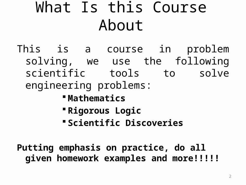
What Is this Course About

This is a course in problem solving, we use the following scientific tools to solve engineering problems:

Mathematics Rigorous Logic Scientific Discoveries

Putting emphasis on practice, do all given homework examples and more!!!!!

3

Revise the Following Scientific Concepts

• Scalar quantities – magnitude only• Vector quantities – magnitude and direction• Integration - General• Differentiation (The Chain Rule)

4

An Overview of Mechanics

Statics: The study of bodies in equilibrium.

Dynamics:1. Kinematics – analysis of motion of bodies considering geometric aspects like displacement, velocity, acceleration2. Kinetics - analysis of forces causing motion of bodies

Mechanics: The study of how bodies react to forces acting on them.

5

Types of Motion

• Rectilinear Motion (Topic for today): motion along a straight-line path. This motion can be analyzed using the Rectangular Coordinate System (x-y-z axes)

• Curvilinear Motion: motion when a particle moves along a curved path. This can be analyzed using:

(i) Rectangular Coordinates (ii) Normal and Tangential Coordinates (iii) Cylindrical Coordinates

6

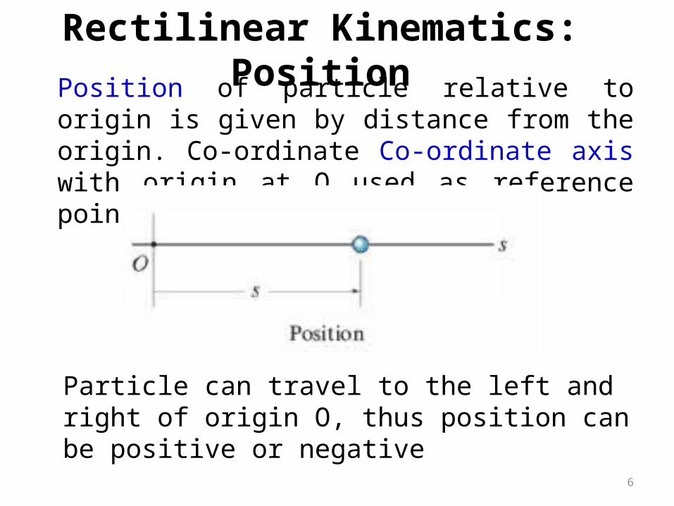
Rectilinear Kinematics: PositionPosition of particle relative to origin is given by distance from the origin. Co-ordinate Co-ordinate axis with origin at O used as reference point.

Particle can travel to the left and right of origin O, thus position can be positive or negative

7

Rectilinear Kinematics: Displacement

The total distance traveled by the particle, sT represents the total length of the path over which the particle travels.

The displacement of the particle is the change in position of the particle relative its original position

s = s’ – s , it can be positive or negative

8

Rectilinear Kinematics: VelocityVelocity is a measure of the rate of change in the position of a particle. It is a vector quantity (it has both magnitude and direction). The magnitude of the velocity is called speed, with units of m/s

Average speed is the total distance traveled divided by elapsed time: (vsp)avg = sT / t

The average velocity of a particle during a time interval t is vavg = s / t

The instantaneous velocity is the time-derivative of position.v = ds / dt

9

Rectilinear Kinematics: Acceleration

Acceleration is the rate of change in the velocity of a particle. Typical units are m/s2.

By manipulating displacement and velocity equations wrt time (t) the following equation is obtainable

ds = v dv

The instantaneous acceleration is the time derivative of velocity. a = dv / dt

Acceleration can be positive (speed increasing) or

negative (speed decreasing).

10

Rectilinear Kinematics: Equations of Motion

Three equations of used to solve problems involving kinematic linear motion.

Integrating the above equation underlying equations obtained

11

12

Example 1

Spotting a police car you brake your car from a speed of 100km/h to a speed of 80km/h during a displacement of 88m at a constant acceleration.

a) What is the acceleration

b) How much time is required to decrease the speed

13

Example 12.5 Textbook

14

PracticeRevise fundamental Scientific concepts

Read pages 1 - 32

Fundamental Problems - All

Problems 12.1 – 12.712.17 – 12.2012.29 – 12.3112.41 - 12.4012.42 – 12.5012.65 – 12.70

15

Curvilinear Kinematics: General MotionApplication

The path of motion of a plane can be tracked with radar and its x, y, and z coordinates (relative to a point on earth) recorded as a function of time.

How can we determine the velocity or acceleration of the plane at any instant?

16

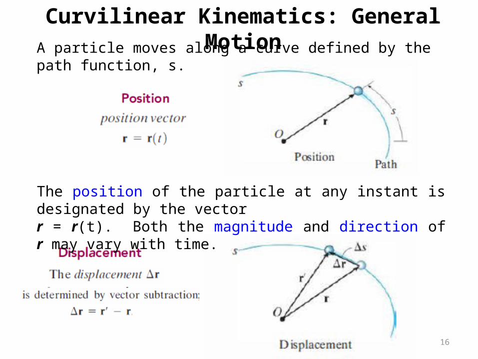
Curvilinear Kinematics: General MotionA particle moves along a curve defined by the path function, s.

The position of the particle at any instant is designated by the vectorr = r(t). Both the magnitude and direction of r may vary with time.

17

Curvilinear Kinematics: General MotionVelocity

As ∆t 0 the direction of ∆r approaches the tangent to the curve. The direction of v(instantaneous) is thus tangential to the curve

The magnitude of v is called the speed, as ∆t 0

Velocity represents the rate of change in the position of a particle.

18

Curvilinear Kinematics: General MotionAcceleration

Acceleration represents the rate of change in the velocity of a particle.

19

Curvilinear Kinematics: Rectangular Co-ordinatesPosition

20

Curvilinear Kinematics: Rectangular Co-ordinatesVelocity

The velocity vector is the time derivative of the position vector:

21

Curvilinear Kinematics: Rectangular Co-ordinatesAcceleration

The acceleration vector is the time derivative of the velocity vector (second derivative of the position vector):

22

Example

The curvilinear motion of a particle is defined by vx = 50 – 16t (meters/second) and y = 100 – 4t2 (meters). The position of x = 0 at t = 0. Plot the path of the particle and determine it’s velocity and acceleration when the position y=0 is reached

23

24

Curvilinear Kinematics: Projectile MotionApplication

25

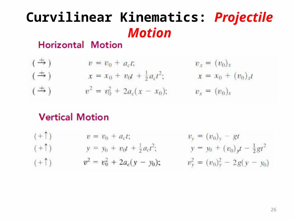
Curvilinear Kinematics: Projectile MotionProjectile motion can be treated as two rectilinear motions, one in the horizontal direction experiencing zero acceleration and the other in the vertical direction experiencing constant acceleration (i.e., from gravity). Since ax = 0, the velocity in the horizontal direction remains constant (vx = vox)

26

Curvilinear Kinematics: Projectile Motion

27

Example

A rocket has expended all its fuel when it reaches position A, where it has a velocity u at an angle with respect to the horizontal. It then begins unpowered flight and attains a maximum added height h at position B after traveling a horizontal distance s from A. Determine the expressions for h and s, the time t of flight from A to B, and the equation of the path. Assume g for gravitational acceleration!

28

Practice

Read pages 32 - 52

Fundamental Problems - All

Problems 12.81 – 12.8312.89 – 12.9112.94 – 12.9712.107 - 12.109

29

Curvilinear Kinematics: Normal & Tangential ComponentsApplication

Cars traveling along a clover-leaf interchange experience an acceleration due to a change in velocity as well as due to a change in direction of the velocity.

If the car’s speed is increasing at a known rate as it travels along a curve, how can we determine the magnitude and direction of its total acceleration?

Why would you care about the total acceleration of the car?

30

Curvilinear Kinematics: Normal & Tangential Components

When a particle moves along a curved path, it is sometimes convenient to describe its motion using coordinates other than Cartesian. When the path of motion is known, normal (n) and tangential (t) coordinates are often used.

In the n-t coordinate system, the origin is located on the particle (the origin moves with the particle).

The t-axis is tangent to the path (curve) at the instant considered, positive in the direction of the particle’s motion.The n-axis is perpendicular to the t-axis with the positive direction toward the center of curvature of the curve.

31

Curvilinear Kinematics: Normal & Tangential ComponentsPosition

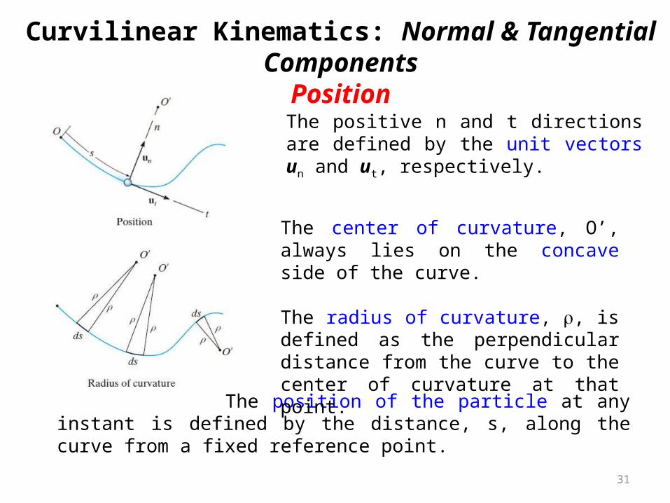
The position of the particle at any instant is defined by the distance, s, along the curve from a fixed reference point.

The positive n and t directions are defined by the unit vectors un and ut, respectively.

The center of curvature, O’, always lies on the concave side of the curve.

The radius of curvature, r, is defined as the perpendicular distance from the curve to the center of curvature at that point.

32

The velocity vector is always tangent to the path of motion (t-direction).

The magnitude is determined by taking the time derivative of the path function, s(t)

where

Here v defines the magnitude of the velocity (speed) andut defines the direction of the velocity vector.

Curvilinear Kinematics: Normal & Tangential ComponentsVelocity

33

Curvilinear Kinematics: Normal & Tangential ComponentsAcceleration

Acceleration is the time rate of change of velocity

Here v represents the change in the magnitude of velocity and ut represents the rate of change in the direction of ut.

After mathematical manipulation, the acceleration vector can be expressed as:

Homework:Understand mathematical manipulation!!!!

34

So, there are two components to the acceleration vector:

a = at ut + an un

• The normal or centripetal component is always directed toward the center of curvature of the curve.

• The tangential component is tangent to the curve and in the direction of increasing or decreasing velocity.

• The magnitude of the acceleration vector is

Curvilinear Kinematics: Normal & Tangential ComponentsAcceleration

35

Curvilinear Kinematics: Normal & Tangential ComponentsSpecial Cases of Motion

There are some special cases of motion to consider.

1) The particle moves along a straight line.r => an = v2/ = 0 =>r a = at = v

The tangential component represents the time rate of change in the magnitude of the velocity.

.

2) The particle moves along a curve at constant speed. at = v = 0 => a = an = v2/r

.

The normal component represents the time rate of change in the direction of the velocity.

36

Curvilinear Kinematics: Normal & Tangential ComponentsSpecial Cases of Motion

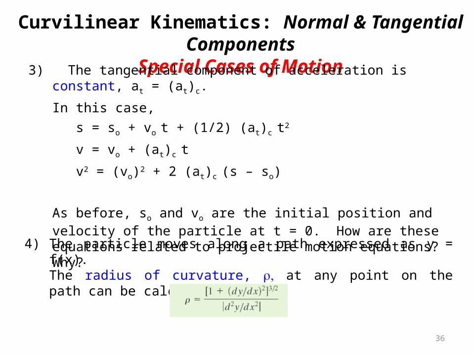
3) The tangential component of acceleration is constant, at = (at)c.

In this case, s = so + vo t + (1/2) (at)c t2

v = vo + (at)c t

v2 = (vo)2 + 2 (at)c (s – so)

As before, so and vo are the initial position and velocity of the particle at t = 0. How are these equations related to projectile motion equations? Why?

4) The particle moves along a path expressed as y = f(x).The radius of curvature, ,r at any point on the path can be calculated from

37

Example

Given: A boat travels around a circular path, r = 40 m, at a speed that increases with time, v = (0.0625 t2) m/s.

Find: The magnitudes of the boat’s velocity and acceleration at the instant t = 10 s.

38

Example

39

Practice

Read pages 52 - 67

Fundamental Problems - All

Problems 12.111 – 12.11412.125 – 12.12712.131– 12.13512.150 - 12.151

40

Curvilinear Kinematics: Cylindrical Co-ordinatesPosition

We can express the location of P in polar coordinates as r = r ur. Note that the radial direction, r, extends outward from the fixed origin, O, and the transverse coordinate, ,q is measured counter-clockwise from the horizontal (in degrees or radians).

Sometimes if motion of a particle is constrained to circular movement, the motion is best described by polar co-ordinates

Positive direction of r and q is defined by unit vectors ur and uq

Radial co-ordinate

41

Curvilinear Kinematics: Cylindrical Co-ordinatesVelocity

Thus, the velocity vector has two components: r, called the radial component, and rq called the transverse component. The speed of the particle at any given instant is given by:

Homework: The mathematical derivation of V

The instantaneous velocity (V) at a point is the first derivative of the radial distance r:

42

Curvilinear Kinematics: Cylindrical Co-ordinatesVelocity

The radial component Vr, is measure of the increase of decrease in radial distance r.

The transverse component Vq can be interpreted as the rate of motion along a circumference having a radius r.

The direction of V is tangent to the path

The angular velocity (in rad/s) is described by the following equation:

43

Curvilinear Kinematics: Cylindrical Co-ordinatesAcceleration

The instantaneous acceleration (a) at a point is the first derivative of the velocity (V):

Homework: The mathematical derivation of a

44

Example

Given: A tracking radar lies in the vertical plane of the path of a rocket which is coasting in unpowered flight above the atmosphere. For the instant when q = 30o the tracking data gives r = 8x104 m , r = 1200 m/s and q = 0.8deg/s. Take gravitational acceleration (g) = 9.2 m/s2

Find: The speed at that particular instant

r

q

..

..

..

45

Example

46

Example

47

Practice

Read pages 67 - 80

Fundamental Problems - All

Problems 12.158 – 12.16212.171 – 12.17312.192 – 12.194

48

Constraint Motion of Interconnected Particles Application

The cable and pulley system shown can be used to modify the speed of the mine car, A, relative to the speed of the motor, M.

It is important to establish the relationships between the various motions in order to determine the power requirements for the motor and the tension in the cable.

For instance, if the speed of the cable (P) is known because we know the motor characteristics, how can we determine the speed of the mine car? Will the slope of the track have any impact on the answer?

49

In many kinematics problems, the motion of one object will depend on the motion of another object.

The motion of each block can be related mathematically by defining position coordinates, sA and sB. Each coordinate axis is defined from a fixed point or datum line, measured positive along each plane in the direction of motion of each block.

The blocks in this figure are connected by an inextensible cord wrapped around a pulley. If block A moves downward along the inclined plane, block B will move up the other incline.

Constraint Motion of Interconnected Particles Position

50

Constraint Motion of Interconnected Particles Position

In this example, position coordinates sA and sB can be defined from fixed datum lines extending from the center of the pulley along each incline to blocks A and B.

If the cord has a fixed length, the position coordinates sA and sB are related mathematically by the equation

sA + lCD + sB = lT

Here lT is the total cord length and lCD is the length of cord passing over the arc CD on the pulley.

51

Constraint Motion of Interconnected Particles Velocity / Acceleration

The negative sign indicates that as A moves down the incline (positive sA direction), B moves up the incline (negative sB direction).

Accelerations can be found by differentiating the velocity expression.

The velocities of blocks A and B can be related by differentiating the position equation. Note that lCD and lT remain constant, so dlCD/dt = dlT/dt = 0

52

Constraint Motion of Interconnected Particles Example

Consider a more complicated example. Position coordinates (sA and sB) are defined from fixed datum lines, measured along the direction of motion of each block.

Note that sB is only defined to the center of the pulley above block B, since this block moves with the pulley. Also, h is a constant.

The red colored segments of the cord remain constant in length during motion of the blocks.

53

Constraint Motion of Interconnected Particles Example

The position coordinates are related by the equation

2sB + h + sA = lT

Where lT is the total cord length minus the lengths of the red segments.

Since lT and h remain constant during the motion, the velocities and accelerations can be related by two successive time derivatives:

2vB = -vA and 2aB = -aA

When block B moves downward (+sB), block A moves to the left (-sA). Remember to be consistent with your sign convention!

54

Constraint Motion of Interconnected Particles Example

This example can also be worked by defining the position coordinate for B (sB) from the bottom pulley instead of the top pulley.

The position, velocity, and acceleration relations then become

2(h – sB) + h + sA = lT

and 2vB = vA 2aB = aA

Prove to yourself that the results are the same, even if the sign conventions are different than the previous formulation.

55

Constraint Motion of Interconnected Particles Procedures for Analysis

These procedures can be used to relate the dependent motion of particles moving along rectilinear paths (only the magnitudes of velocity and acceleration change, not their line of direction).

4. Differentiate the position coordinate equation(s) to relate velocities and accelerations. Keep track of signs!

3. If a system contains more than one cord, relate the position of a point on one cord to a point on another cord. Separate equations are written for each cord.

2. Relate the position coordinates to the cord length. Segments of cord that do not change in length during the motion may be left out.

1. Define position coordinates from fixed datum lines, along the path of each particle. Different datum lines can be used for each particle.

56

Example

Given: In the figure on the left, the cord at A is pulled down with a speed of 2 m/s.

Find: The speed of block B.

Plan:

There are two cords involved in the motion in this example. There will be two position equations (one for each cord). Write these two equations, combine them, and then differentiate them.

57

Example

58

Practice

Read pages 80 - 100

Fundamental Problems - All

Problems 12.202 – 12.20412.209 – 12.210

59

Relative Motion (Translating Axes)Application

If the aircraft carrier is underway with a forward velocity of 50 km/hr and plane A takes off at a horizontal air speed of 200 km/hr (measured by someone on the water), how do we find the velocity of the plane relative to the carrier?

How would you find the same thing for airplane B?

How does the wind impact this sort of situation?

When fighter jets take off or land on an aircraft carrier, the velocity of the carrier becomes an issue.

60

Relative Motion (Translating Axes)Relative Position

The absolute position of two particles A and B with respect to the fixed x, y, z reference frame are given by rA and rB. The position of B relative to A is represented by

Therefore, if rB = (10 i + 2 j ) m

and rA = (4 i + 5 j ) m,

then rB/A = (6 i – 3 j ) m.

61

Relative Motion (Translating Axes)Relative Velocity

To determine the relative velocity of B with respect to A, the time derivative of the relative position equation is taken.

vB/A = vB – vA

orvB = vA + vB/A

In these equations, vB and vA are called absolute velocities and vB/A is the relative velocity of B with respect to A.

Note that vB/A = - vA/B .

62

Relative Motion (Translating Axes)Relative Acceleration

The time derivative of the relative velocity equation yields a similar vector relationship between the absolute and relative accelerations of particles A and B.

These derivatives yield: aB/A = aB – aA

or

aB = aA + aB/A

63

Relative Motion (Translating Axes)Problem Solving

Since the relative motion equations are vector equations, problems involving them may be solved in one of two ways.

1. For instance, the velocity vectors in vB = vA + vB/A could be written as two dimensional (2-D) Cartesian vectors and the resulting 2-D scalar component equations solved for up to two unknowns.

2. Alternatively, vector problems can be solved “graphically” by use of trigonometry. This approach usually makes use of the law of sines or the law of cosines.

64

Relative Motion (Translating Axes)Trigonometry

a b

c

C

BA

Since vector addition or subtraction forms a triangle, sine and cosine laws can be applied to solve for relative or absolute velocities and accelerations. As a review, their formulations are provided below.

Law of Cosines: Abccba cos2222 -+=

Baccab cos2222 -+=

Cabbac cos2222 -+=

Law of Sines:C

c

B

b

A

a

sinsinsin==

65

Relative Motion (Translating Axes)Example

Given: vA = 650 km/h vB = 800 km/h

Find: vB/A

Plan:

a) Vector Method: Write vectors vA and vB in Cartesian form, then determine vB – vA

b) Graphical Method: Draw vectors vA and vB from a common point. Apply the laws of sines and cosines to determine vB/A.

66

Relative Motion (Translating Axes)Example

67

Practice

Problems 12.215 – 12.22012.229 – 12.231

68

Relative Motion (Translating Axes)Example