En genetisk algoritme for navigering i arktiske regioner. Thomas Marstrander Master i datateknikk Hovedveileder: Anders Kofod-Petersen, IDI Institutt for datateknikk og informasjonsvitenskap Innlevert: juni 2014 Norges teknisk-naturvitenskapelige universitet

Welcome message from author
This document is posted to help you gain knowledge. Please leave a comment to let me know what you think about it! Share it to your friends and learn new things together.
Transcript
En genetisk algoritme for navigering i arktiske regioner.
Thomas Marstrander
Master i datateknikk
Hovedveileder: Anders Kofod-Petersen, IDI
Institutt for datateknikk og informasjonsvitenskap
Innlevert: juni 2014
Norges teknisk-naturvitenskapelige universitet

Thomas Marstrander
A genetic algorithm for weather rout-ing in Arctic regions.
Master Thesis, Spring 2014
Artificial Intelligence GroupDepartment of Computer and Information ScienceFaculty of Information Technology, Mathematics and Electrical Engineering

i
Abstract
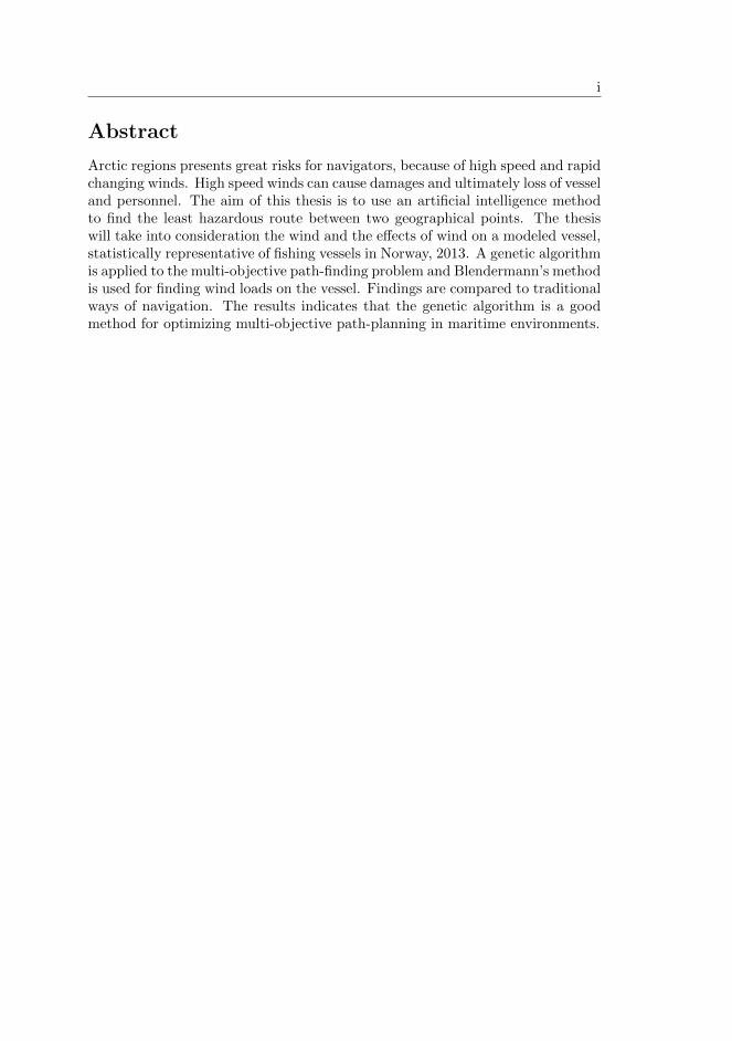
Arctic regions presents great risks for navigators, because of high speed and rapidchanging winds. High speed winds can cause damages and ultimately loss of vesseland personnel. The aim of this thesis is to use an artificial intelligence methodto find the least hazardous route between two geographical points. The thesiswill take into consideration the wind and the effects of wind on a modeled vessel,statistically representative of fishing vessels in Norway, 2013. A genetic algorithmis applied to the multi-objective path-finding problem and Blendermann’s methodis used for finding wind loads on the vessel. Findings are compared to traditionalways of navigation. The results indicates that the genetic algorithm is a goodmethod for optimizing multi-objective path-planning in maritime environments.

ii
Sammendrag
Arktiske omrader innebærer store trusler for navigering, grunnet kraftige og rasktskiftende vinder. Kraftige vinder kan forarsake skader pa personell og fartøy.Malet med tesen er a bruke en kunstig intelligens metode for a finne den tryggesteveien mellom to geografiske koordinater. Tesen analyserer vind og den effektenvind har pa en gitt skipsmodell, som er representativ for fiskebater i Norge i 2013.En genetisk algoritme blir brukt for a løse problemet og Blendermanns metodeer brukt for a finne den effekten vind har pa fartøyet. Resultater fra eksperi-mentering med programmet er sammenlignet med mer tradisjonelle metoder fornavigering. Resultatene fra tesen indikerer at den genetiske algoritmen er en godmetode for a optimalisere en rute i maritime miljø, der flere hensyn kan være ikonflikt med hverandre.

iii
Preface
This thesis is submitted to the Norwegian University of Science and Technology(NTNU) as part of the requirements for fulfilling the degree of Master of Science.
This thesis has been performed for the Department of Computer and InformationScience, NTNU, Trondheim, with Anders Kofod-Petersen as supervisor.
Thomas MarstranderTrondheim, June 26, 2014

iv
Acknowledgements
I would like to thank the whole staff at SINTEF Nord, the managing directorJørn Eldby and co-supervisor Stale Walderhaug for including me in a great workenvironment in Tromsø, and Karl Gunnar Aarsæther for valuable help on mar-itime vessel stability.
I would also like to extend thanks to ”Meteorologisk Institutt” and GunnarNoer for taking interest in my project and providing me with wind data.
Finally, I would like to thank my supervisor at the Department of Computerand Information Science, Anders Kofod-Petersen, for giving me the opportunityto take part in this interesting project and guiding me through it.

v
Abbreviations
GA Genetic Algorithm
GRT Gross Registered Tonnage
HIRLAM High Resolution Limited Area Model
IMO International Maritime Organization
MEWRA Multi Evolutionary Weather Routeing Algorithm
NETCDF Network Common Data Form
RQ Research Question
SAR Synthetic Aperture Radar
SM Systematic Mapping
UML Unified Modeling Language
vi
Symbols
AL Lateral-plane area of a maritime vessel
B Buoyancy centre of a maritime vessel
CK Rolling moment coefficient for a maritime vessel
CY Side-force moment coefficient for a maritime vessel
G Gravity centre of a maritime vessel
GMt Transverse metacentric height of a maritime vessel
HM Mean height of a maritime vessel
K Rolling moment of a maritime vessel
Mt Transverse metacentre of a maritime vessel
R Earth’s radius
SH Lateral-plane centroid above the waterline of a maritime vessel
Y Side-force moment of a maritime vessel
W Displacement of a maritime vessel
g Gravity
ε Wind attack angle in relation to ship
θ Rolling angle of a maritime vessel
ρa Air density
ρw Water density
Contents
1 Introduction 11.1 Objective . . . . . . . . . . . . . . . . . . . . . . . . . . . . . . . . 11.2 Scope . . . . . . . . . . . . . . . . . . . . . . . . . . . . . . . . . . 11.3 Research Goals . . . . . . . . . . . . . . . . . . . . . . . . . . . . . 21.4 Research Method . . . . . . . . . . . . . . . . . . . . . . . . . . . . 3
1.4.1 General Research Approach . . . . . . . . . . . . . . . . . . 31.4.2 Quantification of Simulations . . . . . . . . . . . . . . . . . 3
2 Background and Motivation 52.1 Motivation . . . . . . . . . . . . . . . . . . . . . . . . . . . . . . . 52.2 Best path . . . . . . . . . . . . . . . . . . . . . . . . . . . . . . . . 62.3 Path-finding Algorithms . . . . . . . . . . . . . . . . . . . . . . . . 62.4 Maritime Path-Planning Using Advanced Computations . . . . . . 72.5 Challenges In Maritime Path-Planning . . . . . . . . . . . . . . . . 82.6 Existing Software . . . . . . . . . . . . . . . . . . . . . . . . . . . . 92.7 Refined Problem Description and Scope . . . . . . . . . . . . . . . 10
3 Theory and Methodology 133.1 Meteorological Wind Data . . . . . . . . . . . . . . . . . . . . . . . 13
3.1.1 Representation . . . . . . . . . . . . . . . . . . . . . . . . . 133.1.2 Time-Domain and Area . . . . . . . . . . . . . . . . . . . . 133.1.3 Polar Low . . . . . . . . . . . . . . . . . . . . . . . . . . . . 14
3.2 Ship Model . . . . . . . . . . . . . . . . . . . . . . . . . . . . . . . 163.2.1 Motor . . . . . . . . . . . . . . . . . . . . . . . . . . . . . . 16
3.3 Stability And Physics Overview . . . . . . . . . . . . . . . . . . . . 173.3.1 Simplified Observer Design Model . . . . . . . . . . . . . . 183.3.2 Ship Stability . . . . . . . . . . . . . . . . . . . . . . . . . . 183.3.3 Blendermann’s Method . . . . . . . . . . . . . . . . . . . . 193.3.4 Ship Safety . . . . . . . . . . . . . . . . . . . . . . . . . . . 22
3.4 Distance Calculations . . . . . . . . . . . . . . . . . . . . . . . . . 22
viii Contents
3.4.1 Great Circles . . . . . . . . . . . . . . . . . . . . . . . . . . 233.4.2 Rhumb Line . . . . . . . . . . . . . . . . . . . . . . . . . . . 24
3.5 Genetic Algorithm Theory . . . . . . . . . . . . . . . . . . . . . . . 263.5.1 Multi-Objective Optimization . . . . . . . . . . . . . . . . . 263.5.2 Evolutionary Computing . . . . . . . . . . . . . . . . . . . . 263.5.3 Life-Cycle . . . . . . . . . . . . . . . . . . . . . . . . . . . . 273.5.4 Free Parameters . . . . . . . . . . . . . . . . . . . . . . . . 28
4 Genetic Algorithm Implementation 314.1 Search Space . . . . . . . . . . . . . . . . . . . . . . . . . . . . . . 314.2 Chromosome Representation . . . . . . . . . . . . . . . . . . . . . 324.3 User Input . . . . . . . . . . . . . . . . . . . . . . . . . . . . . . . . 334.4 Solution Space . . . . . . . . . . . . . . . . . . . . . . . . . . . . . 344.5 Initial Population . . . . . . . . . . . . . . . . . . . . . . . . . . . . 354.6 Selection Mechanism . . . . . . . . . . . . . . . . . . . . . . . . . . 354.7 Reproduction and Evolutionary Operators . . . . . . . . . . . . . . 35
4.7.1 Crossover Operation . . . . . . . . . . . . . . . . . . . . . . 374.7.2 Perturb Mutator . . . . . . . . . . . . . . . . . . . . . . . . 374.7.3 Insert Mutator . . . . . . . . . . . . . . . . . . . . . . . . . 374.7.4 Delete Mutator . . . . . . . . . . . . . . . . . . . . . . . . . 384.7.5 Swap Mutator . . . . . . . . . . . . . . . . . . . . . . . . . 384.7.6 Smooth Mutator . . . . . . . . . . . . . . . . . . . . . . . . 384.7.7 Fixed Vector Mutator . . . . . . . . . . . . . . . . . . . . . 39
4.8 Termination . . . . . . . . . . . . . . . . . . . . . . . . . . . . . . . 394.9 Fitness . . . . . . . . . . . . . . . . . . . . . . . . . . . . . . . . . . 39
4.9.1 Distance . . . . . . . . . . . . . . . . . . . . . . . . . . . . . 404.9.2 Maximum Rolling Angle . . . . . . . . . . . . . . . . . . . . 404.9.3 Average Rolling Angle . . . . . . . . . . . . . . . . . . . . . 404.9.4 Time and Fuel Usage . . . . . . . . . . . . . . . . . . . . . . 404.9.5 Maximizing Fitness Features . . . . . . . . . . . . . . . . . 414.9.6 Total Fitness . . . . . . . . . . . . . . . . . . . . . . . . . . 42
4.10 Locations Between Nodes . . . . . . . . . . . . . . . . . . . . . . . 424.11 Wind and Ship Angle Between Two Nodes . . . . . . . . . . . . . . 434.12 Time-Domain . . . . . . . . . . . . . . . . . . . . . . . . . . . . . . 444.13 Result Representation . . . . . . . . . . . . . . . . . . . . . . . . . 444.14 Data Flow of The System . . . . . . . . . . . . . . . . . . . . . . . 45
5 Technical Details 475.1 Experimental Setup . . . . . . . . . . . . . . . . . . . . . . . . . . 475.2 Programming Language . . . . . . . . . . . . . . . . . . . . . . . . 475.3 Wind Data Format . . . . . . . . . . . . . . . . . . . . . . . . . . . 48
Contents ix
5.4 Libraries and Frameworks . . . . . . . . . . . . . . . . . . . . . . . 48
6 Experiments and Results 516.1 Experimental Plan . . . . . . . . . . . . . . . . . . . . . . . . . . . 51
6.1.1 Pre-Algorithm Configuration . . . . . . . . . . . . . . . . . 516.1.2 Phase 1 . . . . . . . . . . . . . . . . . . . . . . . . . . . . . 516.1.3 Phase 2 . . . . . . . . . . . . . . . . . . . . . . . . . . . . . 526.1.4 Phase 3 . . . . . . . . . . . . . . . . . . . . . . . . . . . . . 526.1.5 Phase 4 . . . . . . . . . . . . . . . . . . . . . . . . . . . . . 526.1.6 Phase 5 . . . . . . . . . . . . . . . . . . . . . . . . . . . . . 526.1.7 Phase 6 . . . . . . . . . . . . . . . . . . . . . . . . . . . . . 52
6.2 Scenarios . . . . . . . . . . . . . . . . . . . . . . . . . . . . . . . . 536.2.1 A Normal Route . . . . . . . . . . . . . . . . . . . . . . . . 536.2.2 Polar Low Between Two Nodes . . . . . . . . . . . . . . . . 536.2.3 Path Out of Polar Low . . . . . . . . . . . . . . . . . . . . . 53
6.3 Algorithm Parameters . . . . . . . . . . . . . . . . . . . . . . . . . 536.3.1 Weights . . . . . . . . . . . . . . . . . . . . . . . . . . . . . 536.3.2 Search Space . . . . . . . . . . . . . . . . . . . . . . . . . . 546.3.3 Plotting of Solutions and Graphs . . . . . . . . . . . . . . . 54
6.4 Pre-Algorithm Configurations . . . . . . . . . . . . . . . . . . . . . 546.5 Phase 1 . . . . . . . . . . . . . . . . . . . . . . . . . . . . . . . . . 566.6 Phase 2 . . . . . . . . . . . . . . . . . . . . . . . . . . . . . . . . . 626.7 Phase 3 . . . . . . . . . . . . . . . . . . . . . . . . . . . . . . . . . 676.8 Phase 4 . . . . . . . . . . . . . . . . . . . . . . . . . . . . . . . . . 706.9 Phase 5 . . . . . . . . . . . . . . . . . . . . . . . . . . . . . . . . . 726.10 Phase 6 . . . . . . . . . . . . . . . . . . . . . . . . . . . . . . . . . 73
7 Discussion and Evaluation 777.1 Research Questions . . . . . . . . . . . . . . . . . . . . . . . . . . . 777.2 Discussion . . . . . . . . . . . . . . . . . . . . . . . . . . . . . . . . 78
7.2.1 Rolling Angles . . . . . . . . . . . . . . . . . . . . . . . . . 787.2.2 Phase 4 . . . . . . . . . . . . . . . . . . . . . . . . . . . . . 787.2.3 Selection Mechanisms . . . . . . . . . . . . . . . . . . . . . 797.2.4 Reproducibility of Experiments . . . . . . . . . . . . . . . . 797.2.5 Performance . . . . . . . . . . . . . . . . . . . . . . . . . . 797.2.6 Utility of the algorithm . . . . . . . . . . . . . . . . . . . . 80
7.3 Limitations . . . . . . . . . . . . . . . . . . . . . . . . . . . . . . . 807.3.1 Wind Data . . . . . . . . . . . . . . . . . . . . . . . . . . . 807.3.2 Terrain . . . . . . . . . . . . . . . . . . . . . . . . . . . . . 807.3.3 Blendermann Method Limitations . . . . . . . . . . . . . . 817.3.4 Average Speed . . . . . . . . . . . . . . . . . . . . . . . . . 81
x Contents
7.3.5 Traffic . . . . . . . . . . . . . . . . . . . . . . . . . . . . . . 817.3.6 Weights . . . . . . . . . . . . . . . . . . . . . . . . . . . . . 817.3.7 Time Domain . . . . . . . . . . . . . . . . . . . . . . . . . . 817.3.8 Format . . . . . . . . . . . . . . . . . . . . . . . . . . . . . 827.3.9 On Board Sensors . . . . . . . . . . . . . . . . . . . . . . . 827.3.10 Scalability . . . . . . . . . . . . . . . . . . . . . . . . . . . . 827.3.11 Safety Hazard of Icing on Ships . . . . . . . . . . . . . . . . 82
7.4 Further Work . . . . . . . . . . . . . . . . . . . . . . . . . . . . . . 847.4.1 Higher Resolution Grid . . . . . . . . . . . . . . . . . . . . 847.4.2 Terrain . . . . . . . . . . . . . . . . . . . . . . . . . . . . . 847.4.3 Plotting . . . . . . . . . . . . . . . . . . . . . . . . . . . . . 847.4.4 Redundancy . . . . . . . . . . . . . . . . . . . . . . . . . . . 857.4.5 Evolve Time for Each Node . . . . . . . . . . . . . . . . . . 857.4.6 Risk Curve . . . . . . . . . . . . . . . . . . . . . . . . . . . 857.4.7 Performance . . . . . . . . . . . . . . . . . . . . . . . . . . 85
7.5 Threats to Validity . . . . . . . . . . . . . . . . . . . . . . . . . . . 867.5.1 Time . . . . . . . . . . . . . . . . . . . . . . . . . . . . . . . 867.5.2 Algorithm Performance . . . . . . . . . . . . . . . . . . . . 867.5.3 Diversity . . . . . . . . . . . . . . . . . . . . . . . . . . . . 86
7.6 Evaluation . . . . . . . . . . . . . . . . . . . . . . . . . . . . . . . . 867.6.1 Refine the Topic to a Task . . . . . . . . . . . . . . . . . . . 877.6.2 Design the Method . . . . . . . . . . . . . . . . . . . . . . . 877.6.3 Build a Program . . . . . . . . . . . . . . . . . . . . . . . . 877.6.4 Design Experiments . . . . . . . . . . . . . . . . . . . . . . 877.6.5 Analyze the Experiments and Results . . . . . . . . . . . . 87
8 Conclusion 898.1 Generalization . . . . . . . . . . . . . . . . . . . . . . . . . . . . . 898.2 Contributions To The Research Field . . . . . . . . . . . . . . . . . 90
Bibliography 91
Appendix A: Ship model 95
List of Figures
2.1 Capsize rate of fishing vessels grouped by GRT . . . . . . . . . . . 9
3.1 Wind data area . . . . . . . . . . . . . . . . . . . . . . . . . . . . . 143.2 SAR picture of polar low . . . . . . . . . . . . . . . . . . . . . . . . 153.3 Satellite picture of polar low . . . . . . . . . . . . . . . . . . . . . . 153.4 Plot with wind data barbs . . . . . . . . . . . . . . . . . . . . . . . 163.5 Ship stability considerations . . . . . . . . . . . . . . . . . . . . . . 183.6 Wind forces on a maritime vessel . . . . . . . . . . . . . . . . . . . 203.7 Relation between safety elements . . . . . . . . . . . . . . . . . . . 223.8 Difference between great circle and rhumb line . . . . . . . . . . . 253.9 Genetic Algorithm flowchart . . . . . . . . . . . . . . . . . . . . . . 27
4.1 Modified Search Space . . . . . . . . . . . . . . . . . . . . . . . . . 344.2 Roulette wheel selection . . . . . . . . . . . . . . . . . . . . . . . . 364.3 Evolutionary operators for the GA . . . . . . . . . . . . . . . . . . 364.4 Crossover operation . . . . . . . . . . . . . . . . . . . . . . . . . . 384.5 Wind attack angles . . . . . . . . . . . . . . . . . . . . . . . . . . . 434.6 UML Class Diagram . . . . . . . . . . . . . . . . . . . . . . . . . . 46
6.1 Wind load coefficients . . . . . . . . . . . . . . . . . . . . . . . . . 55(a) Side-force coefficient . . . . . . . . . . . . . . . . . . . . . . . 55(b) Rolling moment coefficient . . . . . . . . . . . . . . . . . . . 55
6.2 Ship lateral plane areal . . . . . . . . . . . . . . . . . . . . . . . . . 556.3 Phase 1 early solutions . . . . . . . . . . . . . . . . . . . . . . . . . 58
(a) Generation 0 . . . . . . . . . . . . . . . . . . . . . . . . . . . 58(b) Generation 1 . . . . . . . . . . . . . . . . . . . . . . . . . . . 58(c) Generation 5 . . . . . . . . . . . . . . . . . . . . . . . . . . . 58
6.4 Phase 1 fitness graph . . . . . . . . . . . . . . . . . . . . . . . . . . 596.5 Phase 1 fitness features . . . . . . . . . . . . . . . . . . . . . . . . 59
(a) Maximum rolling angle . . . . . . . . . . . . . . . . . . . . . 59
xii List of Figures
(b) Distance . . . . . . . . . . . . . . . . . . . . . . . . . . . . . . 596.6 Phase 1 midrun generations . . . . . . . . . . . . . . . . . . . . . . 60
(a) 8. generation . . . . . . . . . . . . . . . . . . . . . . . . . . . 60(b) 10. generation . . . . . . . . . . . . . . . . . . . . . . . . . . 60
6.7 Phase 1 late generations . . . . . . . . . . . . . . . . . . . . . . . . 60(a) 80. generation, local optimum. . . . . . . . . . . . . . . . . . 60(b) 90. generation, escaped local optimum. . . . . . . . . . . . . 60
6.8 Phase 1 final generation . . . . . . . . . . . . . . . . . . . . . . . . 616.9 Phase 1 solution with wind data . . . . . . . . . . . . . . . . . . . 62
(a) at 0 hour. . . . . . . . . . . . . . . . . . . . . . . . . . . . . . 62(b) at 40 hours. . . . . . . . . . . . . . . . . . . . . . . . . . . . . 62(c) at 88 hours. . . . . . . . . . . . . . . . . . . . . . . . . . . . . 62
6.10 Polar low movement . . . . . . . . . . . . . . . . . . . . . . . . . . 63(a) at 0 hour. . . . . . . . . . . . . . . . . . . . . . . . . . . . . . 63(b) at 3 hours. . . . . . . . . . . . . . . . . . . . . . . . . . . . . 63(c) at 6 hours. . . . . . . . . . . . . . . . . . . . . . . . . . . . . 63(d) at 9 hours. . . . . . . . . . . . . . . . . . . . . . . . . . . . . 63
6.11 Phase 2 solution . . . . . . . . . . . . . . . . . . . . . . . . . . . . 65(a) at 0 hour. . . . . . . . . . . . . . . . . . . . . . . . . . . . . . 65(b) at 35 hours. . . . . . . . . . . . . . . . . . . . . . . . . . . . . 65(c) at 70 hours. . . . . . . . . . . . . . . . . . . . . . . . . . . . . 65(d) method comparison. . . . . . . . . . . . . . . . . . . . . . . . 65
6.12 Phase 2 fitness graph . . . . . . . . . . . . . . . . . . . . . . . . . . 666.13 Phase 3 comparison of methods . . . . . . . . . . . . . . . . . . . . 676.14 Phase 3 comparison at different timesteps. . . . . . . . . . . . . . . 69
(a) at 10 hour. . . . . . . . . . . . . . . . . . . . . . . . . . . . . 69(b) at 20 hour. . . . . . . . . . . . . . . . . . . . . . . . . . . . . 69(c) at 30 hour. . . . . . . . . . . . . . . . . . . . . . . . . . . . . 69(d) at 50 hour. . . . . . . . . . . . . . . . . . . . . . . . . . . . . 69
6.15 Phase 4 solution . . . . . . . . . . . . . . . . . . . . . . . . . . . . 716.16 Phase 4 solution close to destination . . . . . . . . . . . . . . . . . 716.17 Phase 5 solution . . . . . . . . . . . . . . . . . . . . . . . . . . . . 736.18 Phase 6 comparison of methods . . . . . . . . . . . . . . . . . . . . 746.19 Phase 6 comparison at different timesteps . . . . . . . . . . . . . . 76
(a) at 1 hour. . . . . . . . . . . . . . . . . . . . . . . . . . . . . . 76(b) at 2 hours. . . . . . . . . . . . . . . . . . . . . . . . . . . . . 76(c) at 3 hours. . . . . . . . . . . . . . . . . . . . . . . . . . . . . 76(d) at 5 hours. . . . . . . . . . . . . . . . . . . . . . . . . . . . . 76(e) at 10 hours. . . . . . . . . . . . . . . . . . . . . . . . . . . . . 76(f) at 15 hours. . . . . . . . . . . . . . . . . . . . . . . . . . . . . 76
List of Tables
3.1 Fishing vessel length . . . . . . . . . . . . . . . . . . . . . . . . . . 173.2 Reference data for Blendermann method . . . . . . . . . . . . . . . 21
6.1 Ship specific data . . . . . . . . . . . . . . . . . . . . . . . . . . . . 566.2 Phase 2 GA and loxodrome comparison . . . . . . . . . . . . . . . 646.3 Phase 2 GA and orthodrome comparison . . . . . . . . . . . . . . . 666.4 Phase 3 GA and loxodrome comparison . . . . . . . . . . . . . . . 686.5 Phase 3 GA and orthodrome comparison . . . . . . . . . . . . . . . 686.6 Phase 4 GA and modified GA comparison . . . . . . . . . . . . . . 726.7 Phase 6 GA, loxodrome and orthodrome comparison . . . . . . . . 746.8 Performance of all phases . . . . . . . . . . . . . . . . . . . . . . . 75

xiv List of Tables
Chapter 1
Introduction
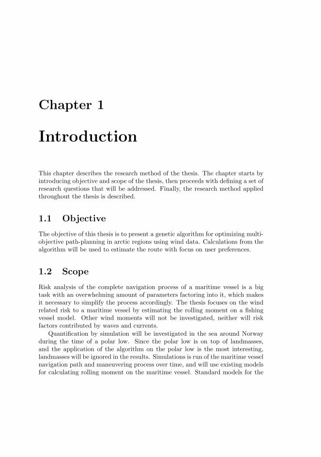
This chapter describes the research method of the thesis. The chapter starts byintroducing objective and scope of the thesis, then proceeds with defining a set ofresearch questions that will be addressed. Finally, the research method appliedthroughout the thesis is described.
1.1 Objective
The objective of this thesis is to present a genetic algorithm for optimizing multi-objective path-planning in arctic regions using wind data. Calculations from thealgorithm will be used to estimate the route with focus on user preferences.
1.2 Scope
Risk analysis of the complete navigation process of a maritime vessel is a bigtask with an overwhelming amount of parameters factoring into it, which makesit necessary to simplify the process accordingly. The thesis focuses on the windrelated risk to a maritime vessel by estimating the rolling moment on a fishingvessel model. Other wind moments will not be investigated, neither will riskfactors contributed by waves and currents.
Quantification by simulation will be investigated in the sea around Norwayduring the time of a polar low. Since the polar low is on top of landmasses,and the application of the algorithm on the polar low is the most interesting,landmasses will be ignored in the results. Simulations is run of the maritime vesselnavigation path and maneuvering process over time, and will use existing modelsfor calculating rolling moment on the maritime vessel. Standard models for the
2 Research Goals
maritime vessel rolling coefficient and angle of rolling will be applied, togetherwith a multi-objective genetic algorithm for minimizing the rolling moment andlength of a path.
The model of navigation will be presented with wind data and geographicaldata, and will not take into account interfering traffic. The resulting paths aredisplayed and compared to more traditional methods, comparing the tradeoffbetween performance of algorithms and desired outcome given specified weightsand parameters.
1.3 Research Goals
For this thesis a main goal is defined, with complementing research questions.
Goal The main goal of this thesis is to develop and study how the genetic al-gorithm can improve on traditional methods for path planning in maritimeenvironments, with focus on wind data.
The goal is defined from a motivation of combining artificial intelligence andmaritime path-planning, with focus on safety. The main goal is complementedby the following research questions, in order to address the various aspects ofdeveloping and testing such an algorithm:
Research question 1 Can a genetic algorithm find an optimal path in a mar-itime environment ?
The first research question is defined to investigate if the genetic algorithmapproach is applicable to the maritime environment. The research question willbe addressed by closely investigating what challenges exists in a maritime en-vironment, and how the GA can deal with these challenges, together with ananalysis of how the genetic algorithm evolves for a specific experiment.
Research question 2 How will the genetic algorithm compare to more tradi-tional methods of path-planning?
The second research question is designed to evaluate the GA against moretraditional methods. Existing methods will be investigated, and the final imple-mentation of the GA will be compared against some of them.
Research question 3 How will the genetic algorithm handle particularly inter-esting applications, such as navigating through a polar low, and navigatingout of a polar low?
Introduction 3
Finally, the third research question deal with the usefulness of the algorithm.Particularly interesting maritime environment scenarios are investigated, and thealgorithm will be applied to these scenarios in order to test the utility of thealgorithm.
1.4 Research Method
Prior to the thesis a specialization project was conducted, which included a lit-erature study using the systematic mapping(SM) method. SM uses thematicanalysis to find patterns and map the literature found. The main findings fromthe specialization project was a gap in artificial intelligence used in maritimepath-planning. There was found no literature on path-planning in relation to thespecial environment in arctic regions, such as the heavy wind in a polar lows.The background theory and design builds on the work done in the specializationproject, and the identified challenges in maritime path-planning.
This thesis implements the genetic algorithm using ideas for design from ear-lier work. The genetic algorithm is implemented iteratively in an agile envi-ronment, while continuously conducting experiment. The latest version shouldalways be a working system.
1.4.1 General Research Approach
The general research approach is conducted in accordance to the quantitativeresearch methodology, the following points are presented in succession throughoutthe thesis:
1. Presentation of models, theories and hypotheses – in chapter 1 and 3.
2. Development and adaption of methods for measurements of experiments –in chapter 4.
3. Experimental control and manipulation of algorithm variables – in chap-ter 6.
4. Collection of empirical simulation data – in chapter 6.
5. Modelling and analysis of the collected data – in chapter 6.
1.4.2 Quantification of Simulations
Quantification of risk by simulations is an established analysis method. The mainresults from the thesis will be through analysis of simulations. The thesis will

4 Research Method
highlight observations of how the algorithm solutions are found, how it performs,and results in comparison to more traditional navigation methods.
Chapter 2
Background and Motivation
This thesis builds on the results of the authors’ specialization project in computerscience, conducted in the fall of 2013. The purpose of this chapter is to providethe necessary background and motivation for this project, and to put the workdone in this thesis in a wider context and in relation to the work of others. Thechapter starts off with a presentation of motivation and background for the thesis,it then proceeds to present the main findings from the specialization project andsimilar research that has been conducted.
2.1 Motivation
Ameeting with representatives from ”Meteorologisk Institutt”1, ”Barentswatch”2,”Yr”3, ”SINTEF Nord”4 and ”Kystverket”5 was held at Kystverket in Tromsøthe 16. October 2013. There was identified an interest for a maritime vesselpath-planning tool that could help ship owners navigate safely in the extremeenvironment that the Arctic regions present.
In Hollnagel [1996] it is identified that a root cause of up to 90% of accidentsis attributed to human elements. In 1983 IMO adopted resolution A.528(13),Recommendation on Weather Routeing, which recognize that routeing advicesuch as ”optimum routes” has proved to benefit ship operations and safety forcrew and cargo, and recommends the usage of weather routeing. This is whythere is a need for computer calculated algorithms, which can aid in the process
1http://www.met.no/2http://www.barentswatch.no/3http://www.yr.no/4http://www.sintef.no/SINTEF-Nord-AS/5http://www.kystverket.no/
6 Best path
of path-planning and finding improvements upon your own route.One of the biggest dangers to maritime vessel, on-board equipment and crew
are when ships rolls too much from side to side. High rolling angles can resultin capsizing, and loss of equipment, vessel and ultimately personnel. Rollingmoment is highly contributed to by wind force on the side of the ship.
In light of the meeting a literature review was conducted to map out the state-of-the-art of maritime navigation, using artificial intelligence methods, in Arcticregions. The research method used in the specialization project was a thematicanalysis of the literature found using systematic mapping, to get an overview ofexisting literature and identifying research gaps. Systematic mapping is struc-tured from a user specified set of search strings applied to a set of databases.The resulting literature is manually filtered iteratively with increasingly strictconstraints. The final set of literature were used as a basis to propose the initialdesign for the multi-objective genetic algorithm used in this thesis.
2.2 Best path
In the past, best paths has been associated with the shortest path. The definitionhas since evolved and is now extended to consider optimizing a given set ofconstraints that is important for traversing the path, e.g. minimizing risk forvessel and crew, least amount of energy consumed and a minimal amount of timeexpended.
Searching for optimal solutions to problems is a common and highly valuedtask both in personal life as well as work environment. People use optimizationwithout even thinking about it to schedule weekly activities. It is also essential inadvanced science and technology, economics and business. Global optimizationis the quest to find the best solution to a problem.
2.3 Path-finding Algorithms
Path-finding algorithms can usually be divided into two categories: pregenerativeand reactive. In pregenerative algorithms the planning is done before the objectstarts traveling, and is without course corrections, as in Chen et al. [1995], whilein reactive algorithms the path is found by the vehicle as it proceeds through theenvironment [Kamon and Rivlin, 1995]. This thesis will focus on the pregenera-tive approach.
There exists many methods for finding optimal paths. In Garau et al. [2005]an application of the A* algorithm is proposed as a search algorithm for pathplanning in the ocean. Energy optimal paths are calculated in a simulated envi-ronment. The most important drawback of this paper is that the ocean currents
Background and Motivation 7
are assumed to be static, wind forces are also not taken into account. An alter-native path-planning based on potential fields are described in Barraquand et al.[1991] and Kwon et al. [2005]. This method works well for avoiding obstacles,but is susceptible to getting stuck at local minima. A comparison between A*search, rapidly-exploring random tree(RTT) and distance transforms is presentedin Jarvis [2006]. Artificial intelligence methods such as case-based reasoning havealso been used in path-planning problems [Vasudevan and Ganesan, 1996], whichhas the benefit of reusing solutions and minimize computational redundancy. Al-varez et al. [2004] provides a genetic algorithm for path planning in strong oceancurrents, and can optimize the route based on several conflicting constraints. Itis shown through rigorous comparisons, that their genetic algorithm producessignificantly superior trajectories than an implementation of particle swarm op-timization in Roberge et al. [2013].
Strong results from genetic algorithms in combination with path-planningproblems, together with the author’s motivation for using the genetic algorithm,resulted in genetic algorithm being the choice of method for solving the path-planning problem in this thesis.
Genetic algorithm uses principles of the Darwinian approach to natural se-lection, and is part of a group of algorithms called evolutionary computing.Evolutionary Computing was made known by Rechenberg [1965] and Holland[1975] by exploiting the mechanics of natural evolution. Today it is used in di-verse artificial intelligence fields such as system optimization, hardware design,computer-assisted manufacturing and robotics, and more described in Floreanoand Mattiussi [2008]. Evolutionary algorithms has the benefit of being able todesign patterns and solutions that are hard for humans to find. A good exampleis the evolved antenna at NASA [Hornby et al., 2006].
In genetic algorithms an initial population of paths are improved iteratively bygenetic operators. Unlike dynamic programming the computational complexityof genetic algorithms increase linearly with the solution space [Petkovi, 2011].The drawback of genetic algorithms is that they can not guarantee an optimalsolution in finite time.
2.4 Maritime Path-Planning Using Advanced Com-putations
As we have seen from the last section there exists many ways of dealing with thepath-planning problem, and they are very general problems. They can be usedin diverse domains, e.g. for aerial vehicles, ships, underwater vehicles, groundrobots and particles, or for routeing data packets in a network.
The primary goal of ship routeing is to reduce a voyage cost in various ways.
8 Challenges In Maritime Path-Planning
From ancient times a captain has been in charge of selecting the best courseusing experience. Maritime vessel weather routeing tries to find an optimumpath for ocean routes based on weather forecast, sea conditions and ship char-acteristics. Finding an optimum path means to focus on important factors, e.g.maximize crew comfort and safety on the voyage, minimize fuel consumption,time and distance used. The maritime navigation problem in Arctic regions isa multi-objective optimization problem, which means finding a compromise be-tween these features that usually are in conflict with each other.
Some of the first work done in complex maritime navigation was done usingthe isochrone method proposed by James [1957]. This method recursively definestime-fronts, finds the best solution for each time front and expands upon these.Several variations of the isochrone method has been proposed since this.
Kobayashi et al. [2011] uses Powell’s method to find an optimal route for fuelexpressed by a bezier curve and calculates the wind coefficients using Fujiwara’smethod. Powell’s method is not very well suited for the problem described in thisthesis because it must be a real-valued function of a fixed number of real-valuedinputs.
The evolutionary approach has been successfully applied in the maritime nav-igation domain. Several implementations of genetic algorithms in optimizationof maritime problem exists, e.g. anti-collision avoidance [Ito et al., 1999], evo-lution of controllers for autonomous vessels [Manley, 2008], traffic organizationin terminals [Smierzchalski, 1999] and cargo stowage problem [Dubrovsky et al.,2002].
A multi-objective version of the evolutionary algorithm, called MEWRA, fornavigation has been applied in Szlapczynska and Smierzchalski [2009], which wasdesigned specifically for a static model hybrid-propulsion ship and execution wasclose to 20 minutes.
2.5 Challenges In Maritime Path-Planning
From the specialization project a set of challenges in relation to path-planningin maritime environment was identified. The challenges can be divided into twogroups, static and dynamic challenges. Static challenges are objects or constraintsthat remains the same throughout traversing the path.Static challenges:
• Canals
• Shallow waters
• Land masses
Background and Motivation 9
• Traffic restricted zones
• Structures, for instance oil rigs or bridges.
Dynamic challenges are objects or fields that change over time:
• Other vessels
• Wind
• Waves
• Currents
• Ice
On a spherical surface, such as the earth, the shortest path between twocoordinates is found by traversing the Great Circle. However if there is storm inthe middle of these coordinates, traveling around the storm can save time andreduce safety risks.
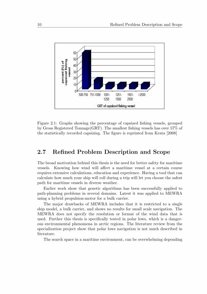
In Krata [2008] it is identified that the first feature influencing the capsizingrate of a vessel is the size of the vessel. Smaller vessels has a higher chance ofcapsizing, as illustrated in figure 2.1.
2.6 Existing Software
A simple google search for ”weather routeing software” provided an overview ofthe weather routeing software that exists today. Following is a list of the softwarethat was found and what kind of method they implement for finding the optimalroute, if specified by the provider:
• QtVlm: isochrone method
• MaxSea: isochrone method
These two softwares and variations of them were the prevailing weather route-ing programs that was found. Several monitoring and onboard-systems were alsofound, however these have different purposes than weather routeing. Both listedprograms use isochrone method. The isochrone method is an old and outdatedway of searching through the solution space, and is prone to ”isochronic loops”as explained in James [1957]. Drawbacks include having to search through thewhole search space for each time front and only allowing for single-objective op-timization.
10 Refined Problem Description and Scope
Figure 2.1: Graphs showing the percentage of capsized fishing vessels, groupedby Gross Registered Tonnage(GRT). The smallest fishing vessels has over 57% ofthe statistically recorded capsizing. The figure is reprinted from Krata [2008]
2.7 Refined Problem Description and Scope
The broad motivation behind this thesis is the need for better safety for maritimevessels. Knowing how wind will affect a maritime vessel at a certain courserequires extensive calculations, education and experience. Having a tool that cancalculate how much your ship will roll during a trip will let you choose the safestpath for maritime vessels in diverse weather.
Earlier work show that genetic algorithms has been successfully applied topath-planning problems in several domains. Latest it was applied to MEWRAusing a hybrid propulsion-motor for a bulk carrier.
The major drawbacks of MEWRA includes that it is restricted to a singleship model, a bulk carrier, and shows no results for small scale navigation. TheMEWRA does not specify the resolution or format of the wind data that isused. Further this thesis is specifically tested in polar lows, which is a danger-ous environmental phenomena in arctic regions. The literature review from thespecialization project show that polar lows navigation is not much described inliterature.
The search space in a maritime environment, can be overwhelming depending
Background and Motivation 11
on the desired precision. Because of this the author wanted to try to use agenetic algorithm, which does not have to search through the complete searchspace in order to find solutions. This thesis takes genetic algorithm in maritimeenvironment a step further by performing extensive experiments in an arcticenvironment, specifically containing a polar low. The ship model is chosen torepresent an especially threatened group of ships, small fishing vessels.
The algorithm focus on safety of the maritime ship model that is chosen inrelevance to wind, and the wind forces that act on ship model. Wind force androlling moment are therefore the main focus of the algorithm, while other dynamicfactors, such as waves and currents are not taken into account.
From the systematic mapping and existing software search there was identi-fied a research gap for artificial intelligence algorithms used with maritime path-planning. This resulted in that the path-planning system had to be developedfrom scratch, using the principles of GA and maritime seakeeping theory.
The outcome of this project includes a working system for computing thesafest path given wind data, and how this path compares to more traditionalmethods of plotting a path. The outcome also includes suggestions for furtherimprovements of the system.

12 Refined Problem Description and Scope
Chapter 3
Theory and Methodology
Predicting stability of maritime vessels and path planning has been and is still amajor research field. A variety of models has been used. The model used in thisresearch is Werner Blendermann’s method for calculating wind loads on ships,which is based on empirical data from extensive testing in wind tunnels. Thischapter contains the meteorological wind data, an overview of the physics actingon a ship, and the method used for implementing the program in this thesis.
3.1 Meteorological Wind Data
The meteorological wind data is essential for calculating the wind forces actingon a maritime vessel, and thus the risk that the windy environment poses to ourmaritime vessel.
3.1.1 Representation
Meteorological data are represented using array-oriented scientific data. The dataprovides a set of geographical locations and corresponding wind in longitudinaldirection and latitudinal direction. Together these form a wind vector at thespecified geographical location. The meteorological data is represented usinga standard scientific data format called netcdf which is explained in detail inchapter 5.
3.1.2 Time-Domain and Area
The time-domain of the data spans from 7.january up to and including 9.january2009, and has measurements for every complete hour, which makes for a total of
14 Meteorological Wind Data
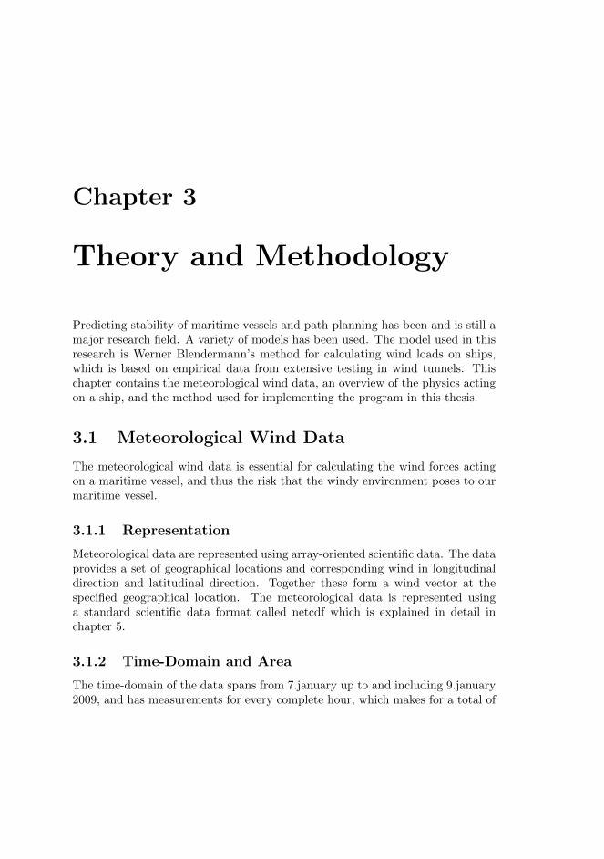
72 timestepsThe geographical zone in which there exists wind data, is limited by geograph-
ical coordinate 43E 003 in the southern corner and 83N 91’30 in the northerncorner, illustrated in figure 3.1.
Figure 3.1: Area containing wind data, limited by 43E 003 in the southern cornerand 83N 91’30 in the northern corner
3.1.3 Polar Low
Polar lows only appear in certain regions of the world during cold air outbreaks,such as the Barents Sea and the Norwegian Sea. A polar low is a low pressuresystem that can contain high speed winds with fast changing directions, whichcan be dangerous to maritime vessels. The reader is reffered to Rasmussen [1979]for a more general discussion of polar lows.
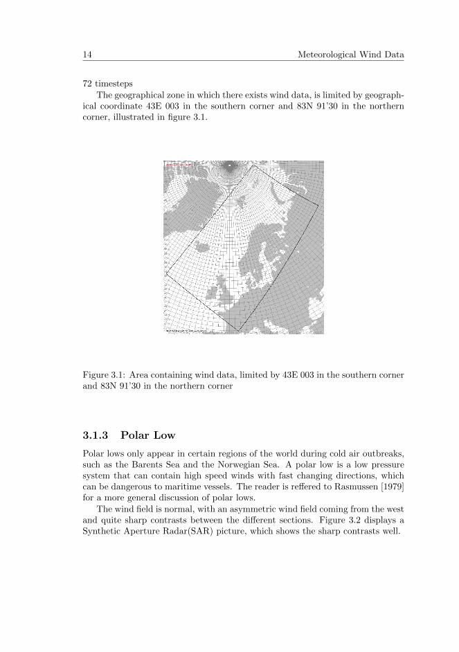
The wind field is normal, with an asymmetric wind field coming from the westand quite sharp contrasts between the different sections. Figure 3.2 displays aSynthetic Aperture Radar(SAR) picture, which shows the sharp contrasts well.
Theory and Methodology 15
Figure 3.2: A SAR picture showng the sharp contrasts of a polar low.
The data is presented using a high resolution limited area model(HIRLAM)8km model, which is an international model for presenting metrological data.This means the resolution set for the zone is 8 kilometers. The whole zone isdivided into a 8km grid with wind measurements at each gridpoint. The wind ismeasured 10 meters above ground level, which is the international standard forclimate measurements.
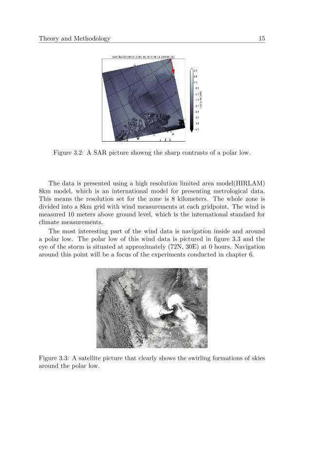
The most interesting part of the wind data is navigation inside and arounda polar low. The polar low of this wind data is pictured in figure 3.3 and theeye of the storm is situated at approximately (72N, 30E) at 0 hours. Navigationaround this point will be a focus of the experiments conducted in chapter 6.
Figure 3.3: A satellite picture that clearly shows the swirling formations of skiesaround the polar low.
16 Ship Model
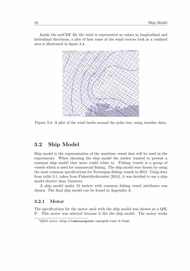
Inside the netCDF file the wind is represented as values in longitudinal andlatitudinal directions, a plot of how some of the wind vectors look in a confinedarea is illustrated in figure 3.4.
Figure 3.4: A plot of the wind barbs around the polar low, using weather data.
3.2 Ship Model
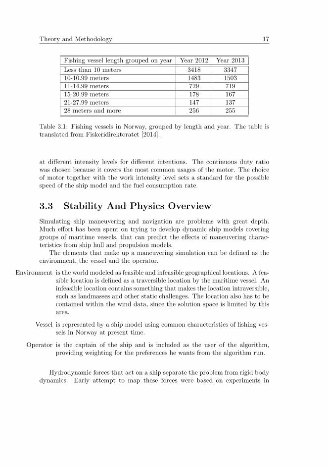
Ship model is the representation of the maritime vessel that will be used in theexperiments. When choosing the ship model the author wanted to present acommon ship model that users could relate to. Fishing vessels is a group ofvessels which is used for commercial fishing. The ship model was chosen by usingthe most common specifications for Norwegian fishing vessels in 2013. Using datafrom table 3.1, taken from Fiskeridirektoratet [2014], it was decided to use a shipmodel shorter than 15meters.
A ship model under 15 meters with common fishing vessel attributes waschosen. The final ship model can be found in Appendix A.
3.2.1 Motor
The specifications for the motor used with the ship model was chosen as a QSL91. This motor was selected because it fits the ship model. The motor works
1QSL9 motor: http://cumminsengines.com/qsl9-tier-4-final
Theory and Methodology 17
Fishing vessel length grouped on year Year 2012 Year 2013
Less than 10 meters 3418 334710-10.99 meters 1483 150311-14.99 meters 729 71915-20.99 meters 178 16721-27.99 meters 147 13728 meters and more 256 255
Table 3.1: Fishing vessels in Norway, grouped by length and year. The table istranslated from Fiskeridirektoratet [2014].
at different intensity levels for different intentions. The continuous duty ratiowas chosen because it covers the most common usages of the motor. The choiceof motor together with the work intensity level sets a standard for the possiblespeed of the ship model and the fuel consumption rate.
3.3 Stability And Physics Overview
Simulating ship maneuvering and navigation are problems with great depth.Much effort has been spent on trying to develop dynamic ship models coveringgroups of maritime vessels, that can predict the effects of maneuvering charac-teristics from ship hull and propulsion models.
The elements that make up a maneuvering simulation can be defined as theenvironment, the vessel and the operator.
Environment is the world modeled as feasible and infeasible geographical locations. A fea-sible location is defined as a traversible location by the maritime vessel. Aninfeasible location contains something that makes the location intraversible,such as landmasses and other static challenges. The location also has to becontained within the wind data, since the solution space is limited by thisarea.
Vessel is represented by a ship model using common characteristics of fishing ves-sels in Norway at present time.
Operator is the captain of the ship and is included as the user of the algorithm,providing weighting for the preferences he wants from the algorithm run.
Hydrodynamic forces that act on a ship separate the problem from rigid bodydynamics. Early attempt to map these forces were based on experiments in
18 Stability And Physics Overview
Norrbin [1971]. A more recent method is captured by performing wind tunneltests on a scale model and determine the wind loads by reference to known valuesof similar ships as in Blendermann [1994]. These models still rely on empiricalformulations for the effects which cannot be captured by the underlying theoryfor the computations.
3.3.1 Simplified Observer Design Model
To simplify the complex nature of forces acting on a ship, an observer designmodel from Fossen [2011] was used. The design is used to observe how shipsbehave in their natural environment. The model includes a disturbance model,where the disturbance is the wind and the goal is to estimate the effect of windon a maritime vessel. Other effects on the vessel, such as currents and waves, isnot taken into consideration. Wind loads, and how they will affect the ship, iscalculated from the Blendermann method. Seakeeping theory is used as a basisfor the calculations. Seakeeping theory refers to the study of ship motion andship stability.
3.3.2 Ship Stability
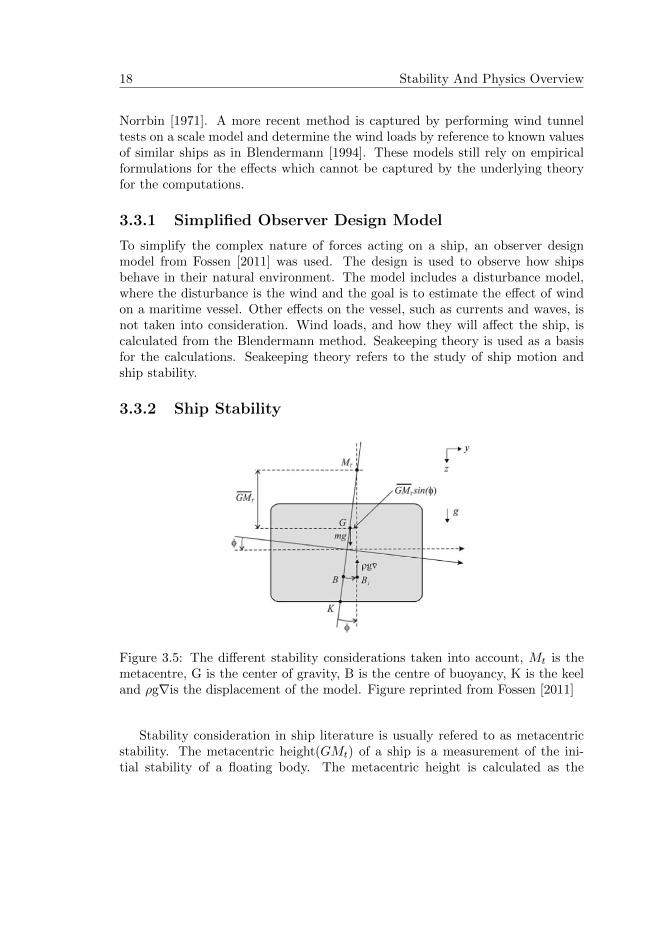
Figure 3.5: The different stability considerations taken into account, Mt is themetacentre, G is the center of gravity, B is the centre of buoyancy, K is the keeland ρg∇is the displacement of the model. Figure reprinted from Fossen [2011]
Stability consideration in ship literature is usually refered to as metacentricstability. The metacentric height(GMt) of a ship is a measurement of the ini-tial stability of a floating body. The metacentric height is calculated as the
Theory and Methodology 19
distance between the centre of gravity(G) of the ship and its’ metacentre (Mt).The metacentre is defined as the point where the vertical of the new centre ofbuoyancy(B) meets the original vertical(B1 through G) through the center ofgravity(G). These values are used for computing the rolling angle (θ) of the ship,which is the amount that the ship will roll from side to side. Increasing rollingangles cause increased discomfort and can ultimately cause the ship to capsize. Infigure 3.5 the different stability considerations of a maritime vessel are illustrated.
When a vessel is effected by an external force the centre of buoyancy B1 isshifted to B and the ship will be tilted to an angle θ. The righting couple is theforce acting to restore the ship to its’ initial equilibrium position. The rightingcouple is defined as:
RightingCouple = ρg∇ ∗GMt ∗ sin(θ) (3.1)
where ρg∇ is the displacement of the ship, comprised of water density, gravityand weight, GMt is the transverse metacentric height and θ is the rolling angleof the ship.
The righting couple, is equal to the external force acting on the ship. Sincethe external forces effecting the ship in this model is the rolling force created bythe wind moment, the righting couple is the same as the rolling moment.
A boat can handle rolling angles up to a certain point where the boat willcapsize. The angle a boat can roll to is strongly decided by the shape, size andcargo of the boat. To calculate the angles with precision a GZ-curve needs to becalculated for every individual boat. The GZ-curve is determined from extensiveexperiments in port. Because this is a rigorous process, not all boats have apre-calculated GZ-curve. Additionally, it would be infeasible to use a GZ-curveas input. An alternative method is therefore used to calculate the stability of aship in this thesis. Using the righting couple to find the rolling angle from therolling moment. Paths that have increasingly high rolling angle are penalized.
Two attributes of a route are of particular interest in regard to stability:
1. Maximum Rolling Angle: This determines how safe the route is to traverse.Less rolling angle means less chance for capsizing and less chance of injuryto crew or equipment.
2. Average Rolling Angle: This determines how comfortable the route is forpassengers and is a particularly important aspect of travel for commercialpassenger ships and leisure trips.
20 Stability And Physics Overview
3.3.3 Blendermann’s Method
To find the rolling angle for a maritime vessel, a method that can calculate therolling moment is needed, as shown in equation 3.1. In Krata [2008] it is suggestedthat the first improvement of the present stability situation, is to get rid of usingthe same stability criterias for vessels of any size.
The method presented in Blendermann [1994] is developed through extensivetesting in wind tunnels for different vessel models, ship hulls and ship character-istics, and provides different stability calculations for vessels of different size.
To calcule the rolling moment of a maritime vessel equation 3.2 is used.
CK =K
ρA ∗AL ∗HM(3.2)
where K is the rolling moment, CK is the rolling moment coefficient, is the airdensity, AL is the lateral area exposed to wind, and HM is the mean height ofthe vessel.
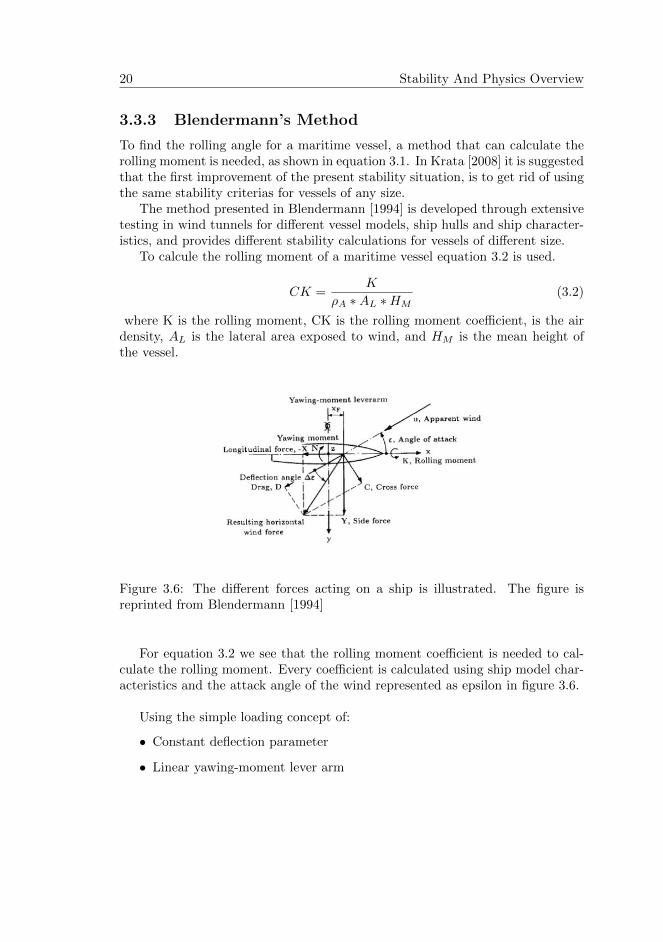
Figure 3.6: The different forces acting on a ship is illustrated. The figure isreprinted from Blendermann [1994]
For equation 3.2 we see that the rolling moment coefficient is needed to cal-culate the rolling moment. Every coefficient is calculated using ship model char-acteristics and the attack angle of the wind represented as epsilon in figure 3.6.
Using the simple loading concept of:
• Constant deflection parameter
• Linear yawing-moment lever arm
Theory and Methodology 21
• Constant rolling-moment lever arm
we get the parametrical loading conditions for calculating the rolling momentcoefficient, as shown in equation 3.3.
CK = κ ∗ SH
HM∗ CY (3.3)
where κis reference data presented in table 3.2, and CY is the side-force coefficientof the maritime vessel.
Equation 3.3 shows that CK is a function of CY, so CY has to be evaluatedfirst, using equation 3.4.
CY = CDt ∗sin2(ε)
1− δ2
∗ (1− CDL
CDt) ∗ sin2(2ε) (3.4)
The coefficients are calculated using the angle of attack from the wind(ε), shipmodel characteristics SH and HM , and reference data from table 3.2.
SH is the position of the lateral-plane centroid above the waterline.HM ismean height, defined by HM = AL
LOA, where AL is the lateral-plane area and LOA
is the length of the areal.
3.3.4 Ship Safety
It is assumed that wind causes the prime safety concern of the maritime vessel.The wind is one cause for icing on a boat and rolling of the boat. It can causediscomfort, safety hazard for the crew and equipment and in some cases capsizing.
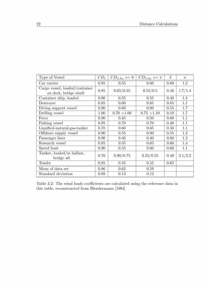
Analysis of historical data has revealed that most accidents is caused by sev-eral elements coinciding at once. The relation between the elements is as a Venndiagram in figure 3.7. There is an increasing risk for accidents, the more elementsthat coincide.
In this thesis, the ship and environment elements are addressed. The captainstill has a big responsibility of overseeing that proper standards are followed sincean increase in cargo loading can induce a list, strong heel and even capsizing.
3.4 Distance Calculations
A path along the surface of the Earth connecting two points is a track. Twotypes of track lines are of interest geographically, great circles and rhumb lines.Great circles represent the shortest possible path between two points. Rhumblines are paths with constant angular headings.
22 Distance Calculations
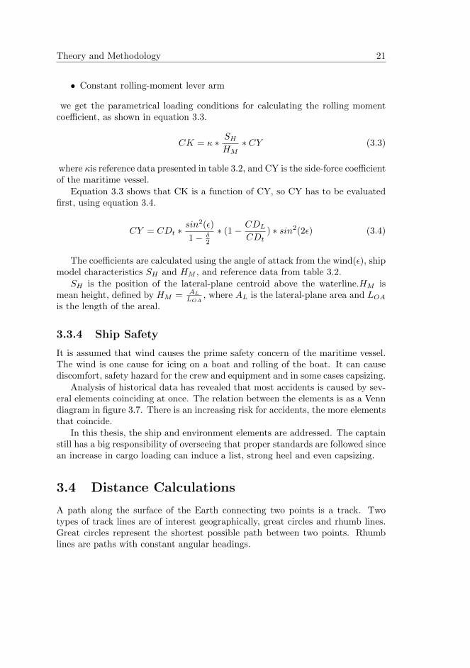
Type of Vessel CDt CDLAFε= 0 CDLAF
ε= π δ κ
Car carrier 0.95 0.55 0.60 0.80 1.2Cargo vessel, loaded/container
on deck, bridge abaft0.85 0.65/0.55 0.55/0.5 0.40 1.7/1.4
Container ship, loaded 0.90 0.55 0.55 0.40 1.4Destroyer 0.85 0.60 0.65 0.65 1.1Diving support vessel 0.90 0.60 0.80 0.55 1.7Drilling vessel 1.00 0.70 ÷1.00 0.75 ÷1.10 0.10 1.7Ferry 0.90 0.45 0.50 0.80 1.1Fishing vessel 0.95 0.70 0.70 0.40 1.1Liquified-natural-gas-tanker 0.70 0.60 0.65 0.50 1.1Offshore supply vessel 0.90 0.55 0.80 0.55 1.2Passenger liner 0.90 0.40 0.40 0.80 1.2Research vessel 0.85 0.55 0.65 0.60 1.4Speed boat 0.90 0.55 0.60 0.60 1.1Tanker, loaded/in ballast,
bridge aft0.70 0.90/0.75 0.55/0.55 0.40 3.1/2.2
Tender 0.85 0.55 0.55 0.65
Mean of data set 0.86 0.62 0.59Standard deviation 0.09 0.13 0.12
Table 3.2: The wind loads coefficients are calculated using the reference data inthis table, reconstructed from Blendermann [1994]
Theory and Methodology 23
Figure 3.7: The relations between elements concerning ship safety are illustratedas a venn diagram. The figure is reprinted from Kobylinski [2007]
3.4.1 Great Circles
A great circle is the shortest path between two points on a sphere. It makes anintersection through the sphere that cuts through both points. The equator andall meridians are great circles. It is not always apparent that the great circle is theshortest path between two points because very few map projections (includingthe mercator projection used in chapter 6) represent great circles as straight lines.
Plotting great circles for navigation is a traditional method of path-planningand is also known as orthodrome navigation method.
The haversine formula is used for finding the great circle distance betweentwo points. It calculates the distance, given the longitudinal and latitudinalcoordinates. The formula for the haversine distance, taken from Sinnott [1984] isshown in equation 3.5.
Haversine distance:
∇λ = λ2 − λ1 (3.5a)
∇φ = φ2 − φ1 (3.5b)
a1 = sin2(∇φ
2
)+ cos(φ1) ∗ cos(φ2) ∗ sin2
(∇λ
2
)(3.5c)
a2 = 2 ∗ arcsin(
min(1,
√a1)
)(3.5d)
d = R ∗ a2 (3.5e)
where λis longitude, φis latitude and R is the radius of the earth, and d is the
24 Distance Calculations
distance between point 1 and 2, defined as (φ1, λ1) and (φ2, λ2) . A sphericalEarth with 6371 kilometer radius is presumed in this thesis.
The formula for finding the mid-point of a great circle is defined in equa-tion 3.6.
Great Circle Midpoint:
b1 = cos(φ2) ∗ cos(∇λ) (3.6a)
b2 = cos(φ2) ∗ sin(∇λ) (3.6b)
φm = atan2(sin(φ1) + sin(φ2),
√(cosφ1 + b1)2 + (b2)2
)(3.6c)
λm = λ1 + atan2(b2, cos(φ1) + b1) (3.6d)
(3.6e)
where λis longitude, φis latitude R is earth’s radius and atan2 is the functiondescribed in equation 3.7. (φm, λm) is the midpoint between (φ1, λ1) and (φ2, λ2).
atan2(y, x) =
arctan( yx ) x > 0
arctan( yx + π) y ≥ 0, x < 0
arctan( yx − π) y < 0, x < 0
+π2 y > 0, x = 0
−π2 y < 0, x = 0
undefined y = 0, x = 0
(3.7)
Way-points in a great circle tracking is found by recursively finding the mid-point of the great circle.
3.4.2 Rhumb Line
A rhumb line, which is also called a loxodrome method of navigation, is a tra-ditional method of navigation. The loxodrome method constructs a curve thatcrosses each meridian at the same angle. All parallels, including the equator,are rhumb lines, since they cross all meridians at 90 degrees. Additionally, allmeridians are rhumb lines, in addition to being great circles.
Plotting a loxodromic path on a mercator map is drawing a straight linebetween two points. Navigating is also easy since you keep the same coursethroughout the whole journey.
The formula for finding the mid-point of a rhumb line is defined in equa-tion 3.8.
Theory and Methodology 25
Rhumb line midpoint:
φm =(φ1 + φ2)
2(3.8a)
c1 = tan
(pi
4+
φ1
2
)(3.8b)
c2 = tan
(π
4+
φ2
2
)(3.8c)
cm = tan
(π
4+
φm
2
)(3.8d)
λm =(λ2λ1) ∗ ln(cm) + λ1 ∗ ln(c2)λ2 ln(c1)
ln( c2c1 )(3.8e)
where λis longitude, φis latitude and ln is natural log. (φm, λm) is the midpointbetween (φ1, λ1) and (φ2, λ2) .
Way-points in a rhumb line tracking is found by recursively applying theequation 3.8.
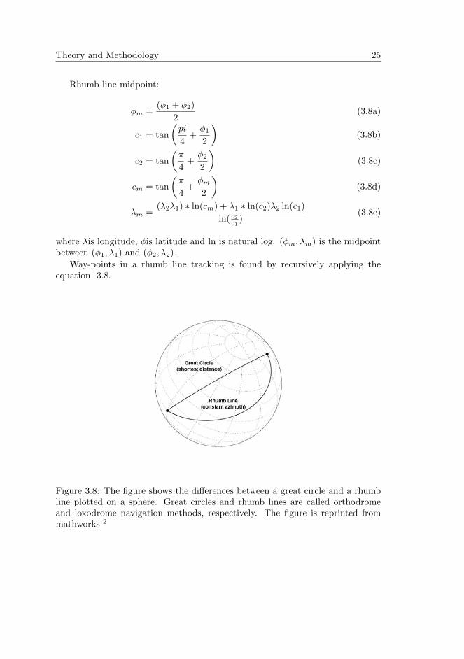
Figure 3.8: The figure shows the differences between a great circle and a rhumbline plotted on a sphere. Great circles and rhumb lines are called orthodromeand loxodrome navigation methods, respectively. The figure is reprinted frommathworks 2
26 Genetic Algorithm Theory
3.5 Genetic Algorithm Theory
3.5.1 Multi-Objective Optimization
When a problem has more than one objective for its’ solution, and these objectivescan be in conflict with each other, the problem becomes increasingly complex. Itis necessary to weight or prioritize the different features of a path in some way.There are three main groups of different multi-objective evolutionary algorithms,separated by how input is processed:
A priori the importance of the parameters are chosen in advance of the runningalgorithm.
A posteriori a pareto-optimal front is found using the algorithm and the choice of se-lecting one of these paths is given to the user.
Alternating the weighting of parameters are done in alternating fashion while runningthe algorithm, usually in the form of questions and computing from these.
A priori is the choice for this algorithm, since it will search through thecomplete search space with the intention of the user from beginning to end.
All optimization problems have inputs, an objective function and output.The input is parameters that describe how the genetic algorithm will run. Theobjective function, also called fitness function, is used to measure the results thatthe algorithm produces and compare the results against eachother. The outputis a solution or set of solutions that are optimal or close to optimal. The goalof optimization is to find an optimal solution within the variable’s bounds, i.e.within the solution space, as in Weise [2009]
3.5.2 Evolutionary Computing
Evolutionary Computing is a group of algorithms which are loosely based onthe Darwinian principles of ”survival of the fittest”. A genetic algorithm is asearch heuristic that is inspired by natural selection. Imagine a species andtheir population. Some individuals have good traits, which is passed down totheir children. The individuals with the best traits carry their genes on, whileindividuals with worse traits eventually die.
The genetic algorithms uses its own solutions and several rules to select thebest solutions and improve upon them through iteration. These kinds of algo-rithms are prefered over mathematical optimization when the solution space issufficiently big and complete knowledge of the domain is not necessarily known.
Genetic algorithms are especially useful in certain situations:
2Great circles, Rhumb lines, and Small circles: http://www.mathworks.se/
Theory and Methodology 27
• The search space is big, complex and poorly understood
• Domain knowledge is scarce and expert knowledge is hard to use for ordi-nary searches
• No adequate mathematical analysis
• Traditional search methods fail
3.5.3 Life-Cycle
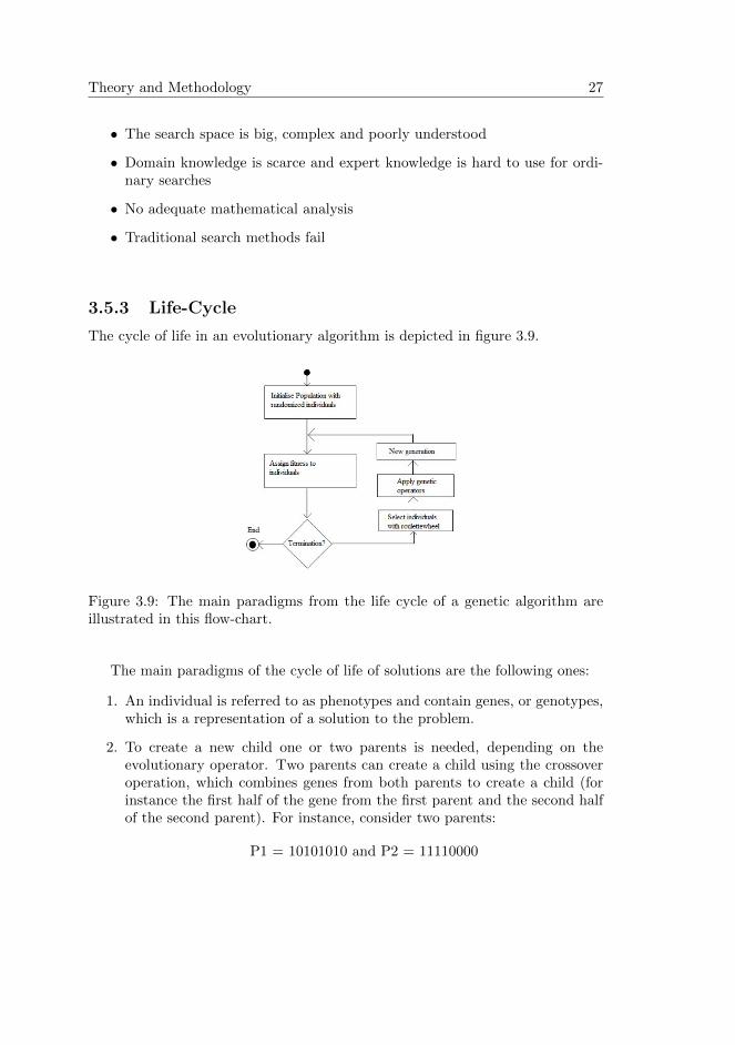
The cycle of life in an evolutionary algorithm is depicted in figure 3.9.
Figure 3.9: The main paradigms from the life cycle of a genetic algorithm areillustrated in this flow-chart.
The main paradigms of the cycle of life of solutions are the following ones:
1. An individual is referred to as phenotypes and contain genes, or genotypes,which is a representation of a solution to the problem.
2. To create a new child one or two parents is needed, depending on theevolutionary operator. Two parents can create a child using the crossoveroperation, which combines genes from both parents to create a child (forinstance the first half of the gene from the first parent and the second halfof the second parent). For instance, consider two parents:
P1 = 10101010 and P2 = 11110000
28 Genetic Algorithm Theory
if the crossover-point is set after point 5 in the genome, then the twochildren are spawned:
C1 = 10100000 and C2 = 11111010
One parent can also create a child alone, this is done by changing parts ofthe parents gene through a mutation operation.
3. There exists a fitness value for every individual which determines the qualityof the individual. Individuals are chosen to be parents through a selectionmechanism, individuals with a high fitness value has higher probability ofbeing chosen for reproduction.
4. The individuals can be removed from a population, their survival is stronglyconnected to their fitness values.
To understand the connection of the genetic algorithm to the biological processjust described, one has to think of the following correspondences on the level ofterminology described in Hromkovic [2010]:
An individual: A feasible solution
A gene: An item of the solution representation
A fitness value: A cost function
A population: A subset of the set of feasible solutions
A mutation: a random local transformation
3.5.4 Free Parameters
Following the concept of the life cycle of a genetic algorithm there are someparameters that has to be set for the concrete implementation of an algorithm.Most of these parameters are connected to a strategy for finding good solutionsat a fast rate:
• Population size
• Selection of initial population
• Fitness function and parent selection mechanism
Theory and Methodology 29
• Representation of individuals and the evolutionary operators
• Stop criterion
Population Size
Selection of population has a certain impact on the run of an algorithm:
1. A small population reduce the diversity of the population. This can resultin that the population converge to a local optimum, which is a solution thatmay be significantly weaker than the fitness of a global optimum.
2. Large populations increase the chance of finding a global optimum.
Having large populations increase the computations for each generation, sothere is important to find a good compromise between the time used for thealgorithm and the quality of the solutions. In general, small population sizesare prefered in order to be competitive with other approaches with respect toalgorithm time complexity.
Selection Of Initial Population
The traditional way to select an initial population is through completely ran-domizing the individuals in a population. Experience has shown that includingpre-computed solutions into the initial population can increase the speed of con-vergence towards good solutions. However, one risk of using only pre-computedsolutions is getting stuck at a local optimum.
Fitness Function And Parent Selection Mechanism
The simplest way to choose fitness for an optimization problem is to give eachindividual an exact fitness value, fitness(individual), which will give each indi-vidual in the population a chance of getting chosen as parents according to thefollowing probability:
p(individual) =fitness(individual)∑
Pi∈Population fitness(Pi)(3.9)
If the probability for most of the individuals in the population is similar, theirprobability of getting selected as parents is similar, resulting in what is calledlow selection pressure. This means even though some individuals are better than
30 Genetic Algorithm Theory
others, there is almost no higher chance of them getting selected as parents. Theprevious shown way of finding parents is called roulette-wheel selection. Anotherway is to rank the individuals according to their fitness and then give themprobability of getting selected for parents from this ranking. This avoids theproblem of similar probability in a population, and is called ranking selection.
Representation Of Individuals And Genetic Operators
The challenge of representating an individual is the same as representing an en-coded solution. The individual has to be constructed so it is possible to changeit easily using evolutionary operators. Some problems, like travelling salesmansproblem(TSP), consider a permutation of 1,2,...,n as the representation of feasi-ble solutions. This representation is not suitable with the crossover operation.Consider these two parents:
P1 = 1 2 3 4 5 6 7 8 and P2 = 2 4 6 8 1 3 5 7
and a crossover operation after point 4, giving the following children:
C1 = 1 2 3 4 1 3 5 7 and C2 = 2 4 6 8 5 6 7 8
where neither of the children represents a permutation of 1,2,3,4,5,6,7,8. Thereare several ways to deal with this, for example allowing solutions that do notrepresent feasible solutions, such as C1 and C2. This can however result inthat the number of individuals that do not represent any feasible solution growsfast. Another solution is to perform the crossover not on the exact solution of theproblem, but on a specifically modified representation of the problem. Whicheverway is chosen to represent the individuals and genetic operators they have to bechosen with great care.
Stop Criterion
The stop criterion determines when the genetic algorithm will terminate with asufficiently good solution. This can be determined in several ways. For instanceif an answer is needed within a specified time, a time criterion can be set, or ifthere is a desire to run the algorithm for a specific number of generations, onecan set a fixed number of generations at the beginning. Another possibility is tomeasure the average fitness of the population at the end of each generation. Ifthe fitness of the population did not change for the last few generations, then thealgorithm can stop. However, if this method is too impatient the run can resultin a local optimum.
Chapter 4
Genetic AlgorithmImplementation
Implementation of the genetic algorithm, which was developed as a main part ofthe master thesis is presented in the following chapter. The genetic algorithmis developed from scratch to solve multi-objective weather routeing between twolocations, with focus on safety related to the rolling angle of a ship model.
4.1 Search Space
The first challenge when implementing an algorithm that works with real worldvalues is the representation of the search space. A real world problem has infiniteamount of coordinates, so the amount of possible coordinates has to be limited insome way. Most traditional path planning algorithms use a search space that iseither graphic-based (for example a roadmap such as google maps) or grid-based(for example cell decomposition) as in Lacki [2008].
Building a search map and searching for a path in it are the main computa-tional tasks in the algorithm. Lacki [2008] arguments that discretized grid modelis the simplest and most efficient way to represent real world problems. For thisproject the search space will consist of a grid constructed from the wind data.This has a predefined resolution for the grid, and the additional benefit that allthe different wind data nodes are reachable and has the same chance of beingchosen.
This also means that the path can only take on the geographical locationsthere are defined wind data for, which is the grid of 8km. The navigation pathcan not take on any geographical locations between the 8km nodes, which may
32 Chromosome Representation
result in a less smooth path than the global optimum. Using this method savescomputational power and simplifies the algorithm search space. The search spaceis shown in figure 3.1.
4.2 Chromosome Representation
For any genetic algorithm the chromosome is the data that will represent a so-lution. The structure of the chromosome lays the foundation for how geneticoperators can be used, and thus how the chromosome can improve. In earlyGAs, the binary digit alphabet was used. Janikow and Michalewicz [1991] hasperformed extensive experiments comparing floating and binary chromosomesand shown that the float-valued chromosomes is faster, provides more precisionand is more concise.
The chromosome is represented as an array of all coordinates that should betraversed by the path, in chronological order. Each index consists of float-valuedcoordinates in the solution space grid, and a state variable. The first and lastnode of the array, which is the origin and destination of the navigation problem,is static and immutable.
The state variable determines whether the specific coordination is feasible. Afeasible grid is traversable and unfeasible grids are not traversable because theycontain land-masses, structures or other hindrances, which makes it impossiblefor a boat to travel through. A path is only feasible if all the locations in the chro-mosome grid is feasible and constructs a path between the origin and destinationof the problem.
Initially it was decided that each coordinate in the chromosome representationhad to be connected to the previous coordinate. During development of thealgorithm it quickly proved that trying to have the algorithm find a path whereevery coordinate had to be connected was infeasible with the computing powerand time constraints at hand. A try with 50 population and 300 generations gaveno feasible paths, and no improvement in feasible nodes, only start node.This ledto a change in the design, allowing ”jumps” from one node to another that wasn’tconnected in the immediate vicinity.
In practice this means that an initially designed path, without every interme-diary node plotted, would be infeasible:
Initial Chromosome (invalid) : [[1,0],[3,0]]
It had to contain the intermediary node [2,0] resulting in this feasible path:
Initial Chromosome (valid) : [[1,0],[2,0],[3,0]]
Genetic Algorithm Implementation 33
Because the initial representations caused crossover and mutation operators tocreate invalid paths most of the time, the final representation of paths was chosenso ”jumping” between nodes are valid paths:
Final Chromosome (valid) : [[1,0],[3,0]]
Because of this representation, there had to be implemented a method to checkevery intermediary node between two coordinates in the path representation fortheir fitness values and feasibility. The revised design allows more paths to befeasible, which means less computation time wasted trying to find feasible pathsand more computation time spent improving the feasible paths.
This representation of the chromosome allow for flexible length, there canbe any number of nodes between the origin and destination node. Allowing forflexible length has the benefit of creating smoother paths and the potential forcomplex path-patterns reliant on wind data.
4.3 User Input
Before starting the algorithm a set of limitations must be set, to specify theproblem for the run. The set of user inputs that needs to be set for each run are:
• Origin
• Destination
• Generations number
• Population size
• Fitness weights
• Ship model
• Wind data
Wind data is the meteorological data that limits the area there exists winddata for, and as a result the search space for the problem. Generations number isthe termination criteria of the algorithm, which determines when the algorithmwill end.
Ship model is the model that will be used in the simulation to traverse theset of paths that are found, and origin and destination defines the problem wherethe ship will travel.
Fitness weights are the weights that are assigned to the different fitness fea-tures of the algorithm, such as distance, maximum rolling angle and average
34 Solution Space
rolling angle.The different weights are chosen from the user’s preferations andintentions. For example a high weight on distance is prefered from an economicalpoint of view, for big boats that can handle big rolling angles. Focus on maxi-mum rolling angle on the other hand is important for small fishing vessels andpassenger boats that can only handle a certain degree of rolling during a voy-age. Average rolling can be of importance for passenger and transport vessels ofpersonnel, where comfort is important. Whichever parameters the user values isinput for the algorithm at the start, so the algorithm knows which way to evolveand what the desired outcome to the run is.
Population size is the amount of individuals a population can contain. A largepopulation size will help diversity of the population since there is bigger chanceof a suboptimal solution within the generation to be carried on. These solutionscan mutate into different optimum than the optimal solution at the present time.
4.4 Solution Space
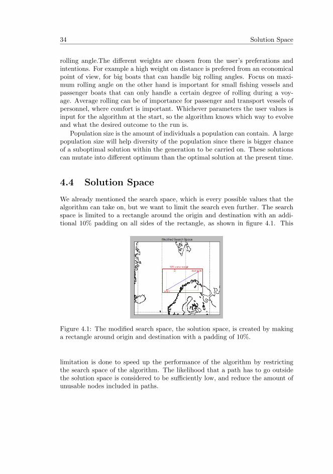
We already mentioned the search space, which is every possible values that thealgorithm can take on, but we want to limit the search even further. The searchspace is limited to a rectangle around the origin and destination with an addi-tional 10% padding on all sides of the rectangle, as shown in figure 4.1. This
Figure 4.1: The modified search space, the solution space, is created by makinga rectangle around origin and destination with a padding of 10%.
limitation is done to speed up the performance of the algorithm by restrictingthe search space of the algorithm. The likelihood that a path has to go outsidethe solution space is considered to be sufficiently low, and reduce the amount ofunusable nodes included in paths.
Genetic Algorithm Implementation 35
4.5 Initial Population
The chromosomes are not completely randomized since they static origin anddestination points. The length of a chromosome is determined as a randomnumber between 1 and length specified in equation 4.1.
ChromosomeMaxLength =√(λdestinationλorigin)2 + (φdestinationφorigin)2 (4.1)
Between the origin and destination there are an amount of intermediary nodescorresponding to the chromosome length number. These nodes are randomizedwithin the solution space. The initial population is created by filling a populationwith randomly created individuals up to the population size.
4.6 Selection Mechanism
In each generation some of the individuals of the population are chosen to get theprivilege of reproduction, and passing their genes on. The fitness value of eachindividual in a population is normalized to the total fitness value of the wholepopulation. The individuals are given a chance of getting chosen equal to theirshare of fitness compared to the rest of the population using equation 3.9.
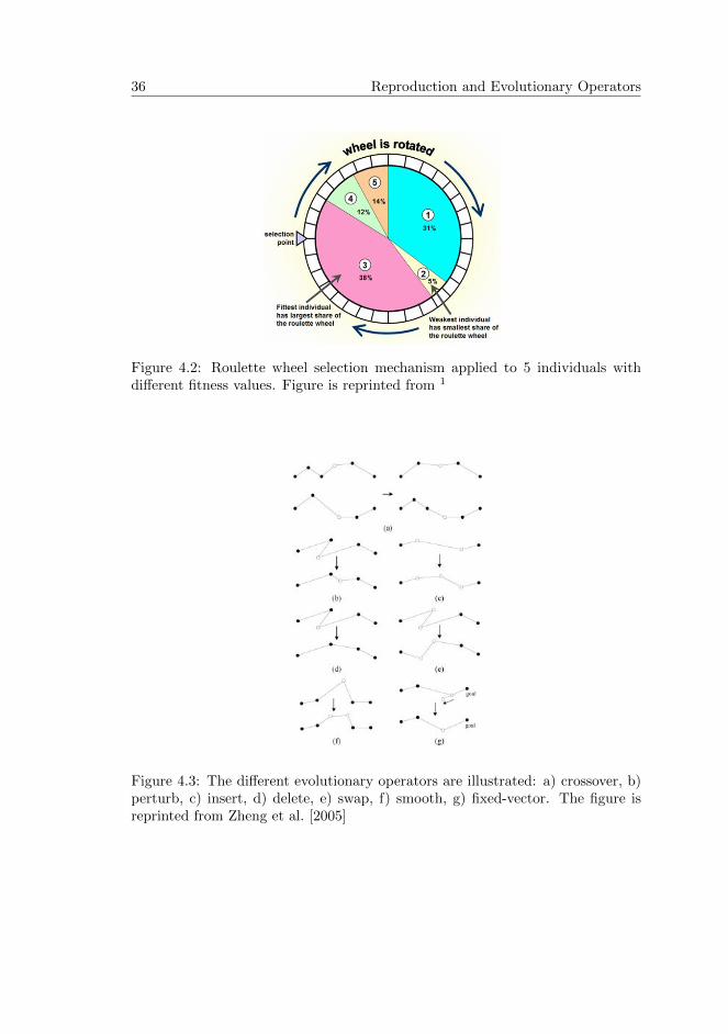
This selection is called fitness-proportionate selection, also known as roulette-wheel selection, and is illustrated in figure 4.2.Each individual is given a per-centage probability on a roulette wheel. The wheel is then spun by choosing arandom value between 0 and 100. The individual that is assigned to the choosenvalue gets to reproduce and carry on its genes. The wheel is spun until a newpopulation, with the user inputted population size of individuals, is chosen.
4.7 Reproduction and Evolutionary Operators
After the selection of individuals that gets to carry on their genes there is thereproduction phase, which consists of crossover operation and mutation operators.Crossover operation produces two new individuals with genetic traits from twochosen parents. Mutation will have genetic traits from one parent together witha mutation that is not inherited, but produced from a randomly chosen operator.The reproduction phase will continue until a new generation has been produced.The new population is then merged with the parents to create the new generation.
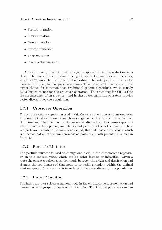
The evolutionary operators that are used in this thesis are shown in figure 4.3,listed and then explained in detail.
• Crossover operation
1Newcastle Engineering Design Centre: http://www.edc.ncl.ac.uk/
36 Reproduction and Evolutionary Operators
Figure 4.2: Roulette wheel selection mechanism applied to 5 individuals withdifferent fitness values. Figure is reprinted from 1
Figure 4.3: The different evolutionary operators are illustrated: a) crossover, b)perturb, c) insert, d) delete, e) swap, f) smooth, g) fixed-vector. The figure isreprinted from Zheng et al. [2005]
Genetic Algorithm Implementation 37
• Perturb mutation
• Insert mutation
• Delete mutation
• Smooth mutation
• Swap mutation
• Fixed-vector mutation
An evolutionary operation will always be applied during reproduction to achild. The chance of an operator being chosen is the same for all operators,which is 1/7, since there are 7 normal operators. The last operator, fixed vectormutator is only applied in special situations. This means that this algorithm hashigher chance for mutation than traditional genetic algorithms, which usuallyhas a higher chance for the crossover operation. The reasoning for this is thatthe chromosomes often are short, and in these cases mutation operators providebetter diversity for the population.
4.7.1 Crossover Operation
The type of crossover operation used in this thesis is a one-point random crossover.This means that two parents are chosen together with a random point in theirchromosomes. The first part of the genotype, divided by the crossover-point istaken from the first parent, and the second part from the other parent. Thesetwo parts are recombined to make a new child, this child has a chromosome whichis a recombination of the two chromosome parts from both parents, as shown infigure 4.4.
4.7.2 Perturb Mutator
The perturb mutator is used to change one node in the chromosome represen-tation to a random value, which can be either feasible or infeasible. Given aroute the operator selects a random node between the origin and destination andchanges the coordinates of that node to something random within the definedsolution space. This operator is introduced to increase diversity in a population.
4.7.3 Insert Mutator
The insert mutator selects a random node in the chromosome representation andinserts a new geographical location at this point. The inserted point is a random
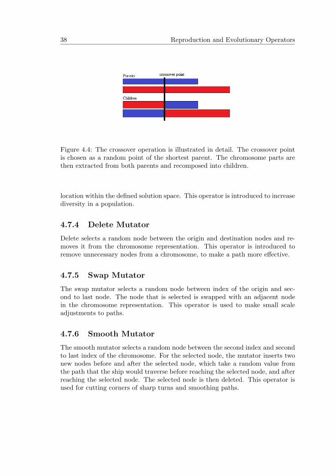
38 Reproduction and Evolutionary Operators
Figure 4.4: The crossover operation is illustrated in detail. The crossover pointis chosen as a random point of the shortest parent. The chromosome parts arethen extracted from both parents and recomposed into children.
location within the defined solution space. This operator is introduced to increasediversity in a population.
4.7.4 Delete Mutator
Delete selects a random node between the origin and destination nodes and re-moves it from the chromosome representation. This operator is introduced toremove unnecessary nodes from a chromosome, to make a path more effective.
4.7.5 Swap Mutator
The swap mutator selects a random node between index of the origin and sec-ond to last node. The node that is selected is swapped with an adjacent nodein the chromosome representation. This operator is used to make small scaleadjustments to paths.
4.7.6 Smooth Mutator
The smooth mutator selects a random node between the second index and secondto last index of the chromosome. For the selected node, the mutator inserts twonew nodes before and after the selected node, which take a random value fromthe path that the ship would traverse before reaching the selected node, and afterreaching the selected node. The selected node is then deleted. This operator isused for cutting corners of sharp turns and smoothing paths.
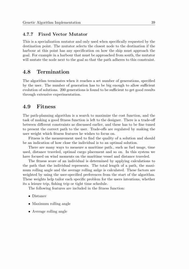
Genetic Algorithm Implementation 39
4.7.7 Fixed Vector Mutator
This is a specialization mutator and only used when specifically requested by thedestination point. The mutator selects the closest node to the destination if theharbour at this point has any specification on how the ship must approach thegoal. For example in a harbour that must be approached from south, the mutatorwill mutate the node next to the goal so that the path adheres to this constraint.
4.8 Termination
The algorithm terminates when it reaches a set number of generations, specifiedby the user. The number of generation has to be big enough to allow sufficientevolution of solutions. 200 generations is found to be sufficient to get good resultsthrough extensive experimentation.
4.9 Fitness
The path-planning algorithm is a search to maximize the cost function, and thetask of making a good fitness function is left to the designer. There is a trade-offbetween different constraints as discussed earlier, and these has to be fine tunedto present the correct path to the user. Trade-offs are regulated by making theuser weight which fitness features he wishes to focus on.
Fitness is the measurement used to find the quality of a solution and shouldbe an indication of how close the individual is to an optimal solution.
There are many ways to measure a maritime path., such as fuel usage, timeused, distance traveled, optimal cargo placement and so on. In this system wehave focused on wind moments on the maritime vessel and distance traveled.
The fitness score of an individual is determined by applying calculations tothe path that the individual represents. The total length of a path, the maxi-mum rolling angle and the average rolling anlge is calculated. These factors areweighted by using the user-specified preferences from the start of the algorithm.These weights help tailor each specific problem for the users intentions, whetherits a leisure trip, fishing trip or tight time schedule.
The following features are included in the fitness function:
• Distance
• Maximum rolling angle
• Average rolling angle
40 Fitness
4.9.1 Distance
The sum of all the distances connecting every node in the chromosome. Thedistance for a complete chromosome is calculate equation 4.2
Distance =
n−1∑i=0
haversine(i, i+ 1) (4.2)
where i ∈ Chromosomenodes, and haversine is described in equation 3.5. Chro-mosomenodes consist of every position that the maritime vessel has to traverseon a path, and will be refered to as Nodes in equations.
4.9.2 Maximum Rolling Angle
This fitness feature measures the rolling angle at every point in a path that achromosome represents. The maximum rolling angle is highest recorded anglewhich a ship will roll from side to side out of all the points that a ship passesthrough. The fitness is calculated using equation 4.3.
MaxRollAngle =∑
i∈Nodes
(max
angle(i)
)(4.3)
where angle(i) is the wind angle at a specific node, found using the Blendermannmethod.
4.9.3 Average Rolling Angle
Similar to the maximum rolling angle fitness feature, this feature measures everyrolling angle that the ship experiences on a path and calculates the average ofthese rolling angles. This fitness feature is calculated using equation 4.4.
AvgRollAngle =
∑i∈Nodes angle(i)
n(4.4)
4.9.4 Time and Fuel Usage
Time used during a path is quite interesting, however in this implementation theaverage speed of a maritime vessel is static, which results in that time used for apath is always equal to:
Time used = distanceaverage speed
Genetic Algorithm Implementation 41
Fuel usage measures the fuel used on the specified path. Since our motor hasa fuel consumption rate of 54L/hr, the fuel is calculated as follows:
fuel consumption = fuel consumption rate * time used
Both of these fitness features are functions of the distance of the path, andsince the distance is already included in the fitness function, fuel usage and timeusage are left out of the final fitness function.
4.9.5 Maximizing Fitness Features
When the maximum rolling angle for a given chromosome is calculated, it is inthe range between 0 and 180 rolling degrees, although a ship will usually capsizeat around 45 degrees, the rest of the values are fictional and a result of theblendermann method of computing the degrees. The maximum rolling angle fora ship is found, by applying the methods in chapter 3 at every location of thechromosome representation. The desired maximum rolling angle is the smallestpossible, however we want to maximize the fitness function. Because of this themaximum rolling angle is normalized against the maximum value it can reach,and then subtracted from 1, so the resulting fitness value of the maximum rollingangle is a value which we want to maximize. The process is shown in equation 4.5
Fitnessmaxrollangle = 1−(MaxRollAngle
180
)(4.5)
Similarly, average rolling angle is a value which should be as small as possible,and is made into a maximizing function using equation 4.6.
Fitnessavgrollangle = 1−(AvgRollAngle
180
)(4.6)
Distance is also a value which should be as small as possible, and is turnedinto a maximizing function by first finding the shortest possible path betweenthe origin and the destination using the haversine, in equation 3.5. The shortestpath is divided on the distance found for this chromosome to find the fitness, asshown in equation 4.7.
Fitnessdistance =haversine(origin, destination)
distance(4.7)
42 Locations Between Nodes
4.9.6 Total Fitness
Now that we have the functions for each fitness feature it is time to put themtogether into a final fitness sum. The total fitness is a sum comprised by thefunctions of fitness features, and should give a good pointer to the quality of thesolution, and how close it is to an optimal solution. This leaves the completefitness function as a set of fitness features and corresponding weights:
Fitness = (fitnessmaxrollangle ∗ weightmaxrollangle)
+ (fitnessavgrollangle ∗ weightavgrollangle)+ (fitnessdistance ∗ weightdistance) (4.8)
where weights are user-specified focus on the different fitness features. Theseweights range from 0 to 1, where 0 is irrelevant weight and 1 is the most importantweight.
4.10 Locations Between Nodes
Since the chromosome only represents the nodes that the algorithm has to visit,it does not contain every point that the vessel has to pass through. To geta complete picture of all the wind forces acting on the maritime vessel, windforce has to be calculated for every point between nodes represented by thechromosome.
To deal with this every actual step that the vessel has to traverse is calculatedby defining stepping values for longitudinal and latitudinal directions between twonodes:
∇φ = φ2 − φ1
∇λ = λ2 − λ1
LonStep =∇φ√
∇φ2 +∇λ2(4.9)
LatStep =∇λ√
∇φ2 +∇λ2(4.10)
where φ is longitude, and λ is latitude.The lonStep and latStep is then applied to the first node. If this increase
in coordinates results in a new grid, the wind forces on the maritime model iscalculated for this grid. These step values are applied iteratively to the newcoordinates, and the wind forces are measured for every new coordinate that is
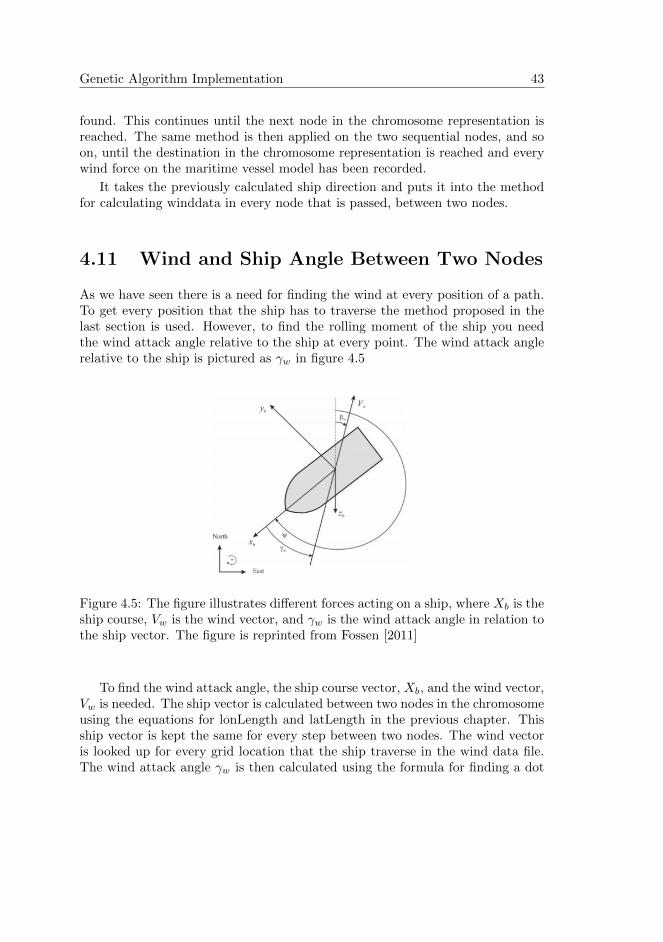
Genetic Algorithm Implementation 43
found. This continues until the next node in the chromosome representation isreached. The same method is then applied on the two sequential nodes, and soon, until the destination in the chromosome representation is reached and everywind force on the maritime vessel model has been recorded.
It takes the previously calculated ship direction and puts it into the methodfor calculating winddata in every node that is passed, between two nodes.
4.11 Wind and Ship Angle Between Two Nodes
As we have seen there is a need for finding the wind at every position of a path.To get every position that the ship has to traverse the method proposed in thelast section is used. However, to find the rolling moment of the ship you needthe wind attack angle relative to the ship at every point. The wind attack anglerelative to the ship is pictured as γw in figure 4.5
Figure 4.5: The figure illustrates different forces acting on a ship, where Xb is theship course, Vw is the wind vector, and γw is the wind attack angle in relation tothe ship vector. The figure is reprinted from Fossen [2011]
To find the wind attack angle, the ship course vector, Xb, and the wind vector,Vw is needed. The ship vector is calculated between two nodes in the chromosomeusing the equations for lonLength and latLength in the previous chapter. Thisship vector is kept the same for every step between two nodes. The wind vectoris looked up for every grid location that the ship traverse in the wind data file.The wind attack angle γw is then calculated using the formula for finding a dot
44 Time-Domain
product between two euclidean vectors shown in equation 4.11.
ShipV ector ∗WindV ector = ||ShipV ector|| ∗ ||WindV ector|| ∗ cos(γw) (4.11)
The resulting wind attack angle is then used used to check against the coef-ficient table produced from using equations 3.4 and 3.3. The coefficient is thenused to find the rolling moment and ultimately the rolling angle of a ship at agiven location using equations 3.2 and 3.1.
A coefficient table is first constructed from the ship model data and a givenprecision for angles, the precision the coefficient table is calculated for every wholerolling angle. This table is then stored in the ship model class of the algorithmfor easy access, since it is accessed for every point that every solution traverses.
4.12 Time-Domain
For the wind data there exists data for different time steps. These are for everywhole hour for 72 hours. One timestep is defined as one hour. If a path exceedsthe maximum time that exists in the wind data, the last record of time data isused to find wind data.
Finding the time for each different point in a chromosome requires to findevery point between the nodes in the chromosome. The length from origin isthen calculated for these points using the haversine formula. The time used atthat point is then found using the:
time used =∑
i∈Nodes Length(i)
AverageShipSpeed
Paths that exceeds the time limitation should usually be purged, because thewind data at these points is not existing. However, most of these results willautomatically be purged by the algorithm because of their long distances, andtime is only dependant on distance. As long as there is some weight on thedistance fitness feature of the algorithm these results will not make it to the finalsolution set.
4.13 Result Representation
The results from the genetic algorithm is the final child and parent generation.These are combined together and then the individual with the highest fitness is
Genetic Algorithm Implementation 45
chosen as the final result. All of the results gathered through the different gen-erations might be interesting to analyse to determine the speed of the algorithm,and how much each generation improves. The following features of a generationis stored in a results file for each run of the algorithm, together with their plots:
The average rolling angle average, max and min values for every generation.
The maximum rolling angle average, max and min values for every genera-tion.
The distance average, max and min values for every generation.
Time used by the system measures the performance of the algorithm
The final path solution with corresponding information
The results file also contains a header with all the input parameters fromthe user, including the fitness features weights, generation number, populationsize, winddata, ship model, origin and destination. After this the rest of theinformation listed is stored in labeled arrays, so they can be extracted at anytime for further analysis.
4.14 Data Flow of The System
Figure 4.6 shows the structure of the genetic algorithm and the main relationsbetween the different classes discussed in this chapter.
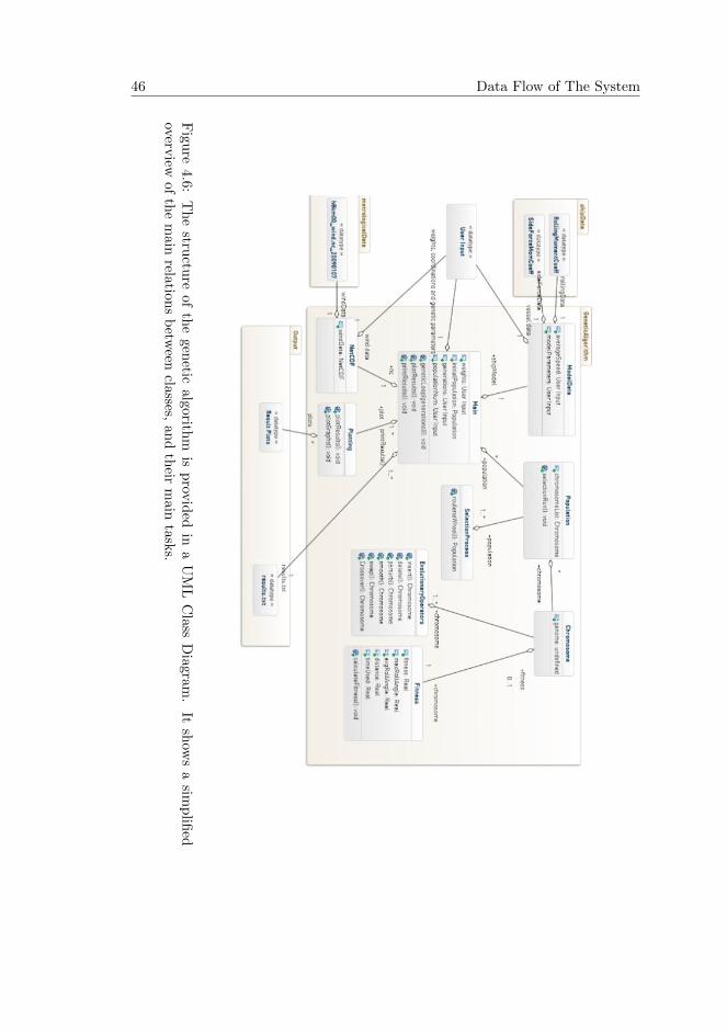
46 Data Flow of The System
Figu
re4.6:
Thestru
cture
ofthegen
eticalgorith
mis
prov
ided
inaUML
Class
Diagram
.It
show
sasim
plifi
edoverv
iewof
themain
relationsbetw
eenclasses,
andtheir
main
tasks.
Chapter 5
Technical Details
The system is built from scratch using the Python programming language. Thischapter lists the experimental setup, the extended frameworks and libraries thatwere used.
5.1 Experimental Setup
The input parameters vary between the experiments and is described at thestart of each result. Two different systems were used for different parts of theexperimenting in chapter experimentsandresults.
System 1 Phases 1 through 4 of the experiments were conducted on a fairly low-performance laptop, Samsung ultrabook with 1.8GHz Intel Core i3-3217Uprocessor, 6GB memory running 64-bit Windows 7.
System 2 Phases 5 and 6 were performed on a dedicated Acer laptop with2.3Ghz Intel Pentium T4500 Dual-Core processor, 2GB memory running64-bit Ubuntu 13.04.
5.2 Programming Language
The source code for the system is written in Python 3.31, an interpreted, inter-active, object-oriented programming language. The code is implemented using
1Python programming language: https://www.python.org/
48 Wind Data Format
the Eclipse ID2 with PyDev3 extension.
5.3 Wind Data Format
The file format that wind data was provided in was NetCDF4.0. NetCDF isan abbrevation for Network Common Data Form, and is a self-describing array-oriented scientific data structure, and widely used for meteorology. Since it is astandard file format for most wind data, the system is designed to have a NetCDFfile as standard input if wind data is going to be used.
5.4 Libraries and Frameworks
The genetic algorithm is implemented from scratch to allow total control of it, andthe necessary extensions needed for the maritime environment. It was assumedthat it could be possible to find suitable and working framework without toomuch effort wasted. Time and effort was redirected to learn these modules,and extending them to some degree, to meet the program requirements. Thisdedication of time was considered a less time-consuming approach than to writesimilar frameworks from scratch.
Matplotlib4 Matplotlib is a python 2D plotting library which produces publi-cation quality figures.Requires the following dependencies:
• PyParsing
• NumPy
• Python-Dateutil
• Six
• Pytz
PyParsing5 PyParsing creates and executes simple python grammars.
NumPy6 NumPy is a fundamental package needed for scientific computing withPython.
2Eclipse IDE: http://www.eclipse.org/3Python Developer: http://pydev.org/4Matplotlib: http://matplotlib.org/5PyParsing: http://pyparsing.wikispaces.com/6NumPy: http://www.numpy.org/

Technical Details 49
Python-Dateutil7 Python-Dateutil provides powerful extensions to the stan-dard datetime module.
Six8 Six is a Python 2 and 3 compatibility library.
Pytz9 Pytz provides world timezones definitions, modern and historical.
NetCDF4-Python10 NetCDF4-Python is a library for reading NetCDF files.Requires:
• HDF5
HDF5 11 HDF5 is a pythonic interface to the HDF5 binary data format.
7Python-Dateutil: http://labix.org/python-dateutil8Six: https://pypi.python.org/pypi/six9Pytz: https://pypi.python.org/pypi/pytz
10NetCDF4-Python: https://code.google.com/p/netcdf4-python/11HDF5: http://www.h5py.org/

50 Libraries and Frameworks
Chapter 6
Experiments and Results
Experiments were performed using the implementation of the genetic algorithmdescribed in chapter 4. The experiments consist of extensive runs for interestingapplications of the algorithm. The chapters starts off with a plan for conductingthe experiments, then provides a description of the scenarios the algorithm istested in. Finally the configurations for the algorithm, and the findings from theresults are presented.
6.1 Experimental Plan
The most interesting application of the algorithm was around and through apolar low. The polar low was close to or on top of land masses. To fully testthe algorithm’s capability in the interesting applications, and due to the lack ofsufficiently detailed terrain data, the landmasses are disregarded in the results.This mean that even if a path is on top of terrain, it is still regarded as a validpath, and is working as intended. The results of the experiments plan are dividedinto phases to cover all research questions. The phases are listed in the followingsection, and the research questions they cover.
6.1.1 Pre-Algorithm Configuration
This phase is conducted to configure ship model, and setting up algorithm to beto handle the wind data.
6.1.2 Phase 1
RQ1 Can a genetic algorithm find an optimal path in the maritime environment?
52 Experimental Plan
To see if the implementation of the algorithm can find an optimal path in mar-itime environment a simple run is executed. The results shows the set of solutionsat different generations to show how the algorithm improves upon the paths, andultimately finds a set of viable solutions.
6.1.3 Phase 2
RQ2 How will the genetic algorithm compare to more traditional methods ofpath-planning?
In the second phase, a path vertically through a polar low is considered. Thealgorithm evolves a path with reduced risk to the maritime vessel, caused bywind forces. It then compares the different fitness features of a path to the moretraditional methods, loxodrome and orthodrome path-finding.
6.1.4 Phase 3
Similar to phase 2, the experiment performed in this phase shows a horizontalpath through a polar low. This experiment reveals the differences between lox-odrome and orthodrome paths more clearly. The genetic algorithm findings isagain compared to the traditional methods, according to RQ2.
6.1.5 Phase 4
RQ3 How will the genetic algorithm handle particularly interesting applications,such as navigating through a polar low, and navigating out of a polar low?
Navigating out of a polar low is a particularly interesting application of thealgorithm. Not much literature exists on how to navigate out of storms, andfinding the safest path could help save lives. This phase attempts to find thesafest path out of a polar low.
6.1.6 Phase 5
In phase 5 a longer run is executed with higher genetic parameters. The pathstarts inside a polar low and escapes to Tromsø.
6.1.7 Phase 6
Phase 6 concludes the final experiment in this thesis and is an extended runusing considerably larger genetic parameters. It escapes the polar low towardsthe west. It uses considerably larger genetic parameters to try to find intricatepatterns through the polar low, evolved over more generations.
Experiments and Results 53
6.2 Scenarios
The different scenarios that are of interest for the application of this algorithm,given the wind data available, are listed in the following section.
6.2.1 A Normal Route
A seemingly safe path over a long distance. This path seems safe at the start ofthe journey, but if we investigate the time-domain it could intersect with a stormat a later point. This scenario will investigate the time domain of the algorithmto see how this will be handled.
6.2.2 Polar Low Between Two Nodes
A path between two geographical locations can have a polar low between them.When having to cross a polar low there arises the question of whether to try toavoid the polar low completely by going all the way around it, or just take thechance of going straight through. Gains by going straight through is a shorterpath distance, but in real environments this does not necessarily translate to lesstime and fuel spent. The gains of taking the longer route around a polar low areprimarily in safety of the ship and crew.
6.2.3 Path Out of Polar Low
This scenario investigates how a path is constructed when a ship is already stuckinside the middle of a storm. In this scenario distance of a path is of littleimportance, and is assigned only a small value to prevent the ship from going incircles or staying at the same location. This scenario is the most dangerous andpaths out of a polar low has to be carefully planned.
6.3 Algorithm Parameters
Before running the algorithm some considerations has to be made, they are ad-dressed in the following section.
6.3.1 Weights
The weights has a big impact on the run of the algorithm. They are specified inadvance of running the algorithm, so the user can decide which fitness features tofocus during each run. The weights are all normalized between 0 and 1 to allowfor desired configuration. For instance a user could specify that he wants to focus
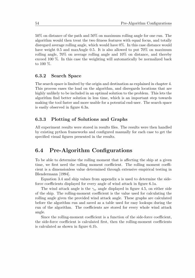
54 Pre-Algorithm Configurations
50% on distance of the path and 50% on maximum rolling angle for one run. Thealgorithm would then treat the two fitness features with equal focus, and totallydisregard average rolling angle, which would have 0%. In this case distance wouldhave weight 0.5 and maxAngle 0.5. It is also allowed to put 70% on maximumrolling angle, 70% on average rolling angle and 10% on distance, and therebyexceed 100 %. In this case the weighting will automatically be normalized backto 100 %.
6.3.2 Search Space
The search space is limited by the origin and destination as explained in chapter 4.This process eases the load on the algorithm, and disregards locations that arehighly unlikely to be included in an optimal solution to the problem. This lets thealgorithm find better solution in less time, which is an important step towardsmaking the tool faster and more usable for a potential end-user. The search spaceis easily observed in figure 6.3a.
6.3.3 Plotting of Solutions and Graphs
All experiment results were stored in results files. The results were then handledby existing python frameworks and configured manually for each case to get thespecified visual figures presented in the results.
6.4 Pre-Algorithm Configurations
To be able to determine the rolling moment that is affecting the ship at a giventime, we first need the rolling moment coefficient. The rolling moment coeffi-cient is a dimensionless value determined through extensive empirical testing inBlendermann [1994].
Equation 3.4 and ship values from appendix a is used to determine the side-force coefficients displayed for every angle of wind attack in figure 6.1a.
The wind attack angle is the γw angle displayed in figure 4.5, on either sideof the ship. The rolling-moment coefficient is the value used for calculating therolling angle given the provided wind attack angle. These graphs are calculatedbefore the algorithm run and saved as a table used for easy lookups during therun of the algorithm. The coefficients are stored for every whole wind attackangle.
Since the rolling-moment coefficient is a function of the side-force coefficient,the side-force coefficient is calculated first, then the rolling-moment coefficientsis calculated as shown in figure 6.1b.
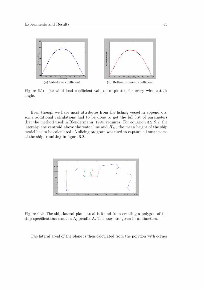
Experiments and Results 55
(a) Side-force coefficient (b) Rolling moment coefficient
Figure 6.1: The wind load coefficient values are plotted for every wind attackangle.
Even though we have most attributes from the fishing vessel in appendix a,some additional calculations had to be done to get the full list of parametersthat the method used in Blendermann [1994] requires. For equation 3.2 SH , thelateral-plane centroid above the water line and HM , the mean height of the shipmodel has to be calculated. A slicing program was used to capture all outer partsof the ship, resulting in figure 6.2.
Figure 6.2: The ship lateral plane areal is found from creating a polygon of theship specifications sheet in Appendix A. The axes are given in millimeters.
The lateral areal of the plane is then calculated from the polygon with corner
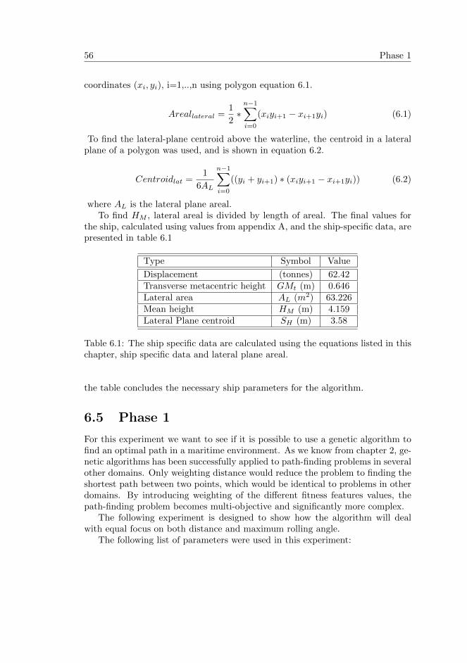
56 Phase 1
coordinates (xi, yi), i=1,..,n using polygon equation 6.1.
Areallateral =1
2∗
n−1∑i=0
(xiyi+1 − xi+1yi) (6.1)
To find the lateral-plane centroid above the waterline, the centroid in a lateralplane of a polygon was used, and is shown in equation 6.2.
Centroidlat =1
6AL
n−1∑i=0
((yi + yi+1) ∗ (xiyi+1 − xi+1yi)) (6.2)
where AL is the lateral plane areal.To find HM , lateral areal is divided by length of areal. The final values for
the ship, calculated using values from appendix A, and the ship-specific data, arepresented in table 6.1
Type Symbol Value
Displacement (tonnes) 62.42Transverse metacentric height GMt (m) 0.646Lateral area AL (m2) 63.226Mean height HM (m) 4.159Lateral Plane centroid SH (m) 3.58
Table 6.1: The ship specific data are calculated using the equations listed in thischapter, ship specific data and lateral plane areal.
the table concludes the necessary ship parameters for the algorithm.
6.5 Phase 1
For this experiment we want to see if it is possible to use a genetic algorithm tofind an optimal path in a maritime environment. As we know from chapter 2, ge-netic algorithms has been successfully applied to path-finding problems in severalother domains. Only weighting distance would reduce the problem to finding theshortest path between two points, which would be identical to problems in otherdomains. By introducing weighting of the different fitness features values, thepath-finding problem becomes multi-objective and significantly more complex.
The following experiment is designed to show how the algorithm will dealwith equal focus on both distance and maximum rolling angle.
The following list of parameters were used in this experiment:
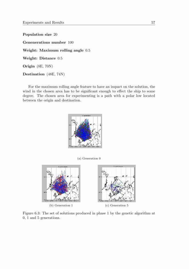
Experiments and Results 57
Population size 20
Genenerations number 100
Weight: Maximum rolling angle 0.5
Weight: Distance 0.5
Origin (8E, 70N)
Destination (48E, 74N)
For the maximum rolling angle feature to have an impact on the solution, thewind in the chosen area has to be significant enough to effect the ship to somedegree. The chosen area for experimenting is a path with a polar low locatedbetween the origin and destination.
(a) Generation 0
(b) Generation 1 (c) Generation 5
Figure 6.3: The set of solutions produced in phase 1 by the genetic algorithm at0, 1 and 5 generations.
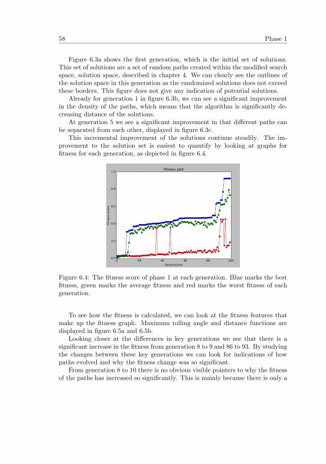
58 Phase 1
Figure 6.3a shows the first generation, which is the initial set of solutions.This set of solutions are a set of random paths created within the modified searchspace, solution space, described in chapter 4. We can clearly see the outlines ofthe solution space in this generation as the randomized solutions does not exceedthese borders. This figure does not give any indication of potential solutions.
Already for generation 1 in figure 6.3b, we can see a significant improvementin the density of the paths, which means that the algorithm is significantly de-creasing distance of the solutions.
At generation 5 we see a significant improvement in that different paths canbe separated from each other, displayed in figure 6.3c.
This incremental improvement of the solutions continue steadily. The im-provement to the solution set is easiest to quantify by looking at graphs forfitness for each generation, as depicted in figure 6.4.
Figure 6.4: The fitness score of phase 1 at each generation. Blue marks the bestfitness, green marks the average fitness and red marks the worst fitness of eachgeneration.
To see how the fitness is calculated, we can look at the fitness features thatmake up the fitness graph. Maximum rolling angle and distance functions aredisplayed in figure 6.5a and 6.5b.
Looking closer at the differences in key generations we see that there is asignificant increase in the fitness from generation 8 to 9 and 86 to 93. By studyingthe changes between these key generations we can look for indications of howpaths evolved and why the fitness change was so significant.
From generation 8 to 10 there is no obvious visible pointers to why the fitnessof the paths has increased so significantly. This is mainly because there is only a
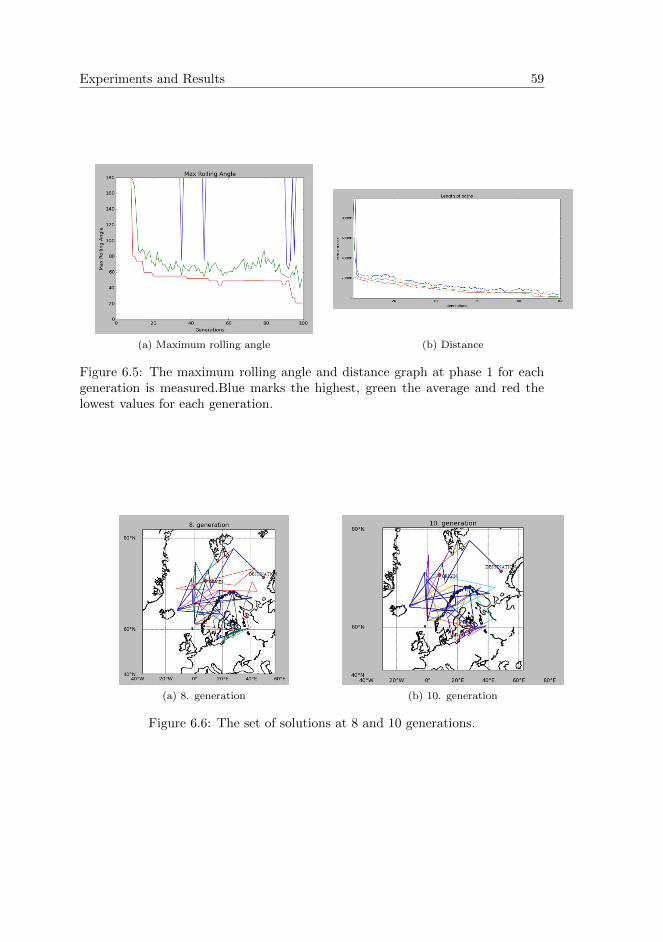
Experiments and Results 59
(a) Maximum rolling angle (b) Distance
Figure 6.5: The maximum rolling angle and distance graph at phase 1 for eachgeneration is measured.Blue marks the highest, green the average and red thelowest values for each generation.
(a) 8. generation (b) 10. generation
Figure 6.6: The set of solutions at 8 and 10 generations.
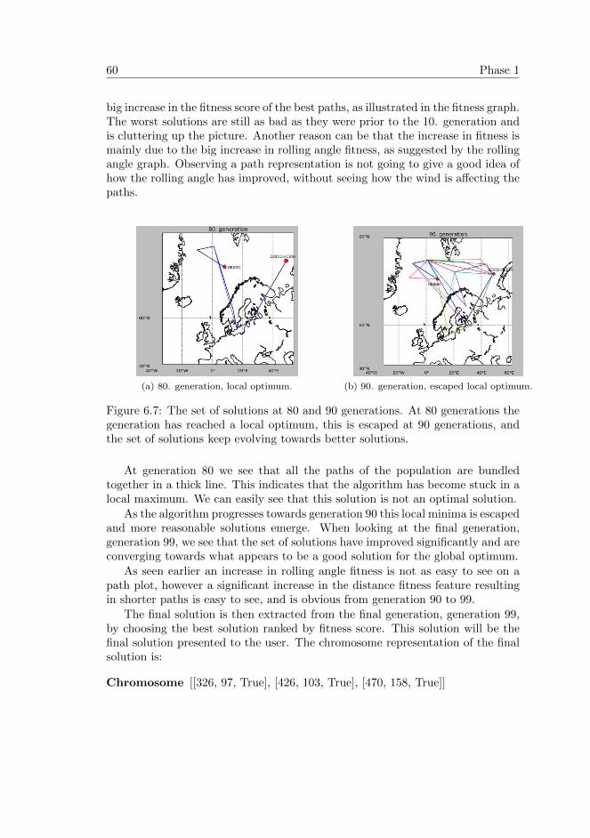
60 Phase 1
big increase in the fitness score of the best paths, as illustrated in the fitness graph.The worst solutions are still as bad as they were prior to the 10. generation andis cluttering up the picture. Another reason can be that the increase in fitness ismainly due to the big increase in rolling angle fitness, as suggested by the rollingangle graph. Observing a path representation is not going to give a good idea ofhow the rolling angle has improved, without seeing how the wind is affecting thepaths.
(a) 80. generation, local optimum. (b) 90. generation, escaped local optimum.
Figure 6.7: The set of solutions at 80 and 90 generations. At 80 generations thegeneration has reached a local optimum, this is escaped at 90 generations, andthe set of solutions keep evolving towards better solutions.
At generation 80 we see that all the paths of the population are bundledtogether in a thick line. This indicates that the algorithm has become stuck in alocal maximum. We can easily see that this solution is not an optimal solution.
As the algorithm progresses towards generation 90 this local minima is escapedand more reasonable solutions emerge. When looking at the final generation,generation 99, we see that the set of solutions have improved significantly and areconverging towards what appears to be a good solution for the global optimum.
As seen earlier an increase in rolling angle fitness is not as easy to see on apath plot, however a significant increase in the distance fitness feature resultingin shorter paths is easy to see, and is obvious from generation 90 to 99.
The final solution is then extracted from the final generation, generation 99,by choosing the best solution ranked by fitness score. This solution will be thefinal solution presented to the user. The chromosome representation of the finalsolution is:
Chromosome [[326, 97, True], [426, 103, True], [470, 158, True]]
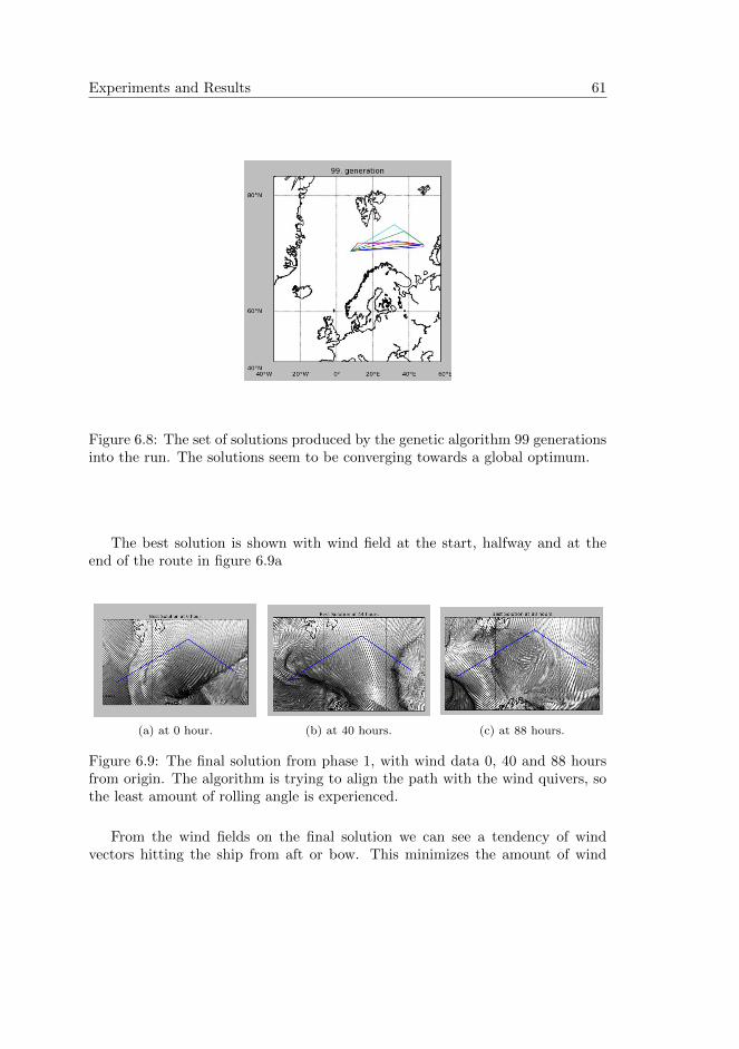
Experiments and Results 61
Figure 6.8: The set of solutions produced by the genetic algorithm 99 generationsinto the run. The solutions seem to be converging towards a global optimum.
The best solution is shown with wind field at the start, halfway and at theend of the route in figure 6.9a
(a) at 0 hour. (b) at 40 hours. (c) at 88 hours.
Figure 6.9: The final solution from phase 1, with wind data 0, 40 and 88 hoursfrom origin. The algorithm is trying to align the path with the wind quivers, sothe least amount of rolling angle is experienced.
From the wind fields on the final solution we can see a tendency of windvectors hitting the ship from aft or bow. This minimizes the amount of wind
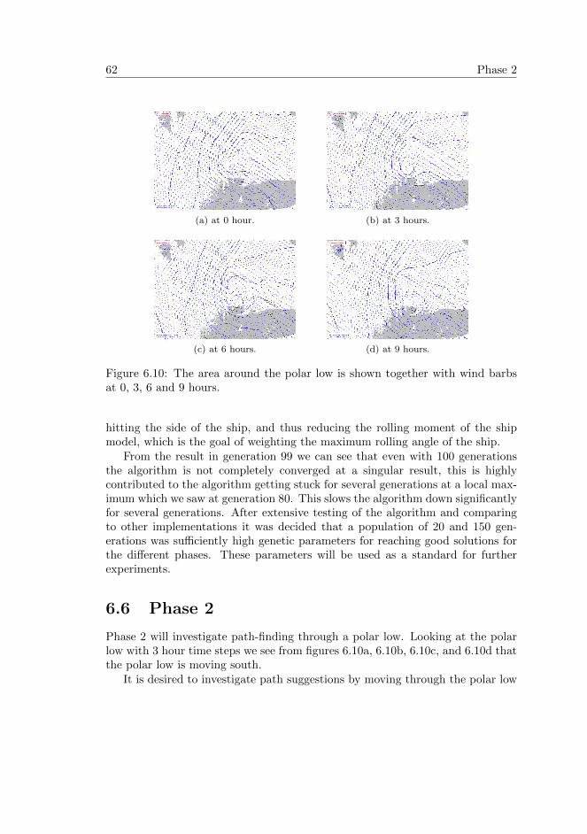
62 Phase 2
(a) at 0 hour. (b) at 3 hours.
(c) at 6 hours. (d) at 9 hours.
Figure 6.10: The area around the polar low is shown together with wind barbsat 0, 3, 6 and 9 hours.
hitting the side of the ship, and thus reducing the rolling moment of the shipmodel, which is the goal of weighting the maximum rolling angle of the ship.
From the result in generation 99 we can see that even with 100 generationsthe algorithm is not completely converged at a singular result, this is highlycontributed to the algorithm getting stuck for several generations at a local max-imum which we saw at generation 80. This slows the algorithm down significantlyfor several generations. After extensive testing of the algorithm and comparingto other implementations it was decided that a population of 20 and 150 gen-erations was sufficiently high genetic parameters for reaching good solutions forthe different phases. These parameters will be used as a standard for furtherexperiments.
6.6 Phase 2
Phase 2 will investigate path-finding through a polar low. Looking at the polarlow with 3 hour time steps we see from figures 6.10a, 6.10b, 6.10c, and 6.10d thatthe polar low is moving south.
It is desired to investigate path suggestions by moving through the polar low
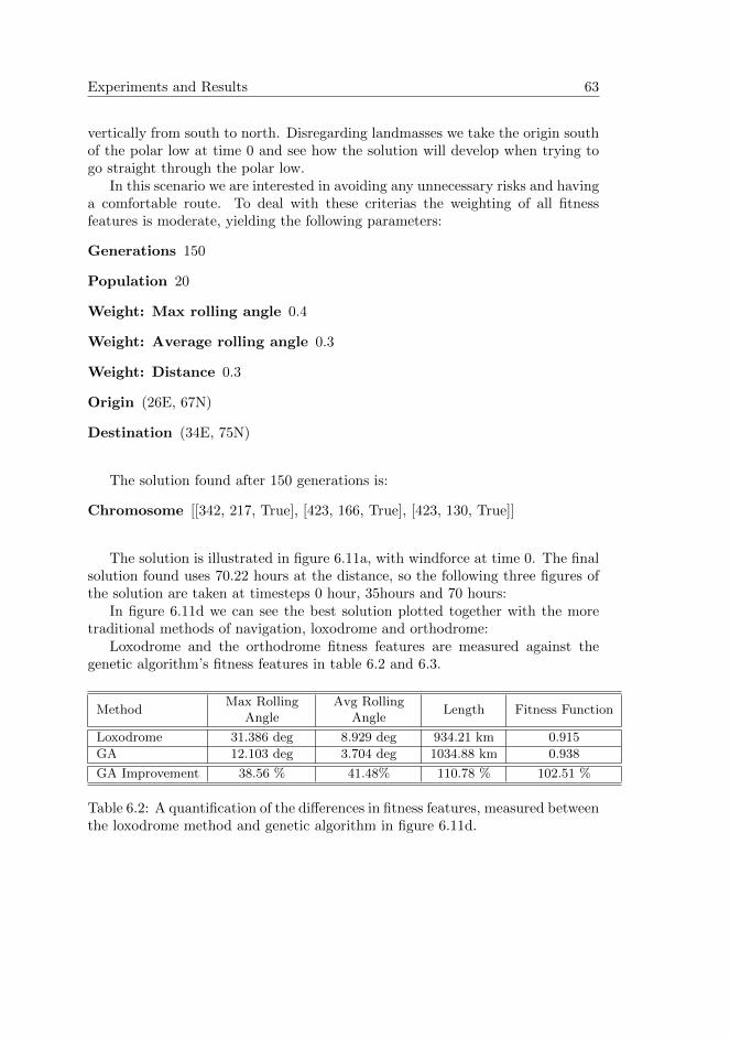
Experiments and Results 63
vertically from south to north. Disregarding landmasses we take the origin southof the polar low at time 0 and see how the solution will develop when trying togo straight through the polar low.
In this scenario we are interested in avoiding any unnecessary risks and havinga comfortable route. To deal with these criterias the weighting of all fitnessfeatures is moderate, yielding the following parameters:
Generations 150
Population 20
Weight: Max rolling angle 0.4
Weight: Average rolling angle 0.3
Weight: Distance 0.3
Origin (26E, 67N)
Destination (34E, 75N)
The solution found after 150 generations is:
Chromosome [[342, 217, True], [423, 166, True], [423, 130, True]]
The solution is illustrated in figure 6.11a, with windforce at time 0. The finalsolution found uses 70.22 hours at the distance, so the following three figures ofthe solution are taken at timesteps 0 hour, 35hours and 70 hours:
In figure 6.11d we can see the best solution plotted together with the moretraditional methods of navigation, loxodrome and orthodrome:
Loxodrome and the orthodrome fitness features are measured against thegenetic algorithm’s fitness features in table 6.2 and 6.3.
MethodMax Rolling
AngleAvg Rolling
AngleLength Fitness Function
Loxodrome 31.386 deg 8.929 deg 934.21 km 0.915
GA 12.103 deg 3.704 deg 1034.88 km 0.938
GA Improvement 38.56 % 41.48% 110.78 % 102.51 %
Table 6.2: A quantification of the differences in fitness features, measured betweenthe loxodrome method and genetic algorithm in figure 6.11d.
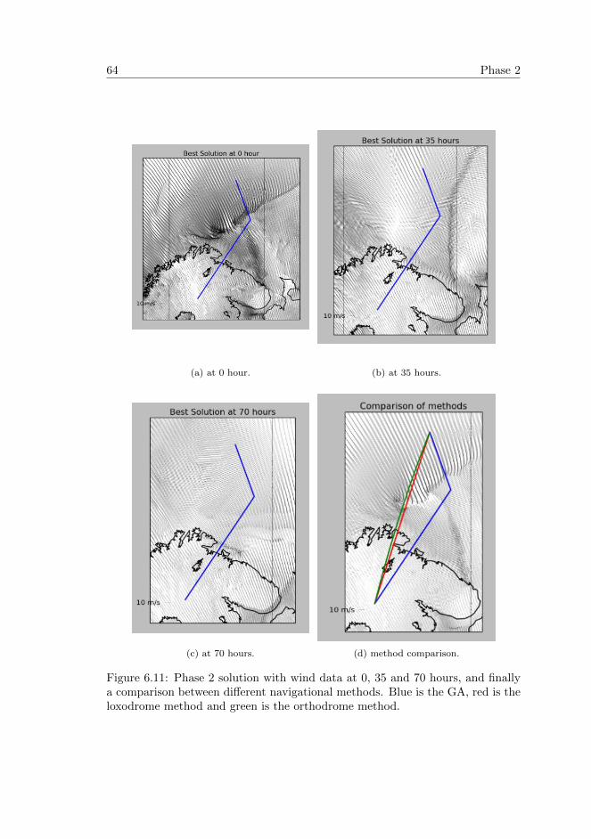
64 Phase 2
(a) at 0 hour. (b) at 35 hours.
(c) at 70 hours. (d) method comparison.
Figure 6.11: Phase 2 solution with wind data at 0, 35 and 70 hours, and finallya comparison between different navigational methods. Blue is the GA, red is theloxodrome method and green is the orthodrome method.
Experiments and Results 65
Figure 6.12: The fitness graph for every generation of the run is illustrated. Blueis the highest fitness, green is the average and red is the lowest for each generation.
We can see that the loxodrome path has over 31 degrees rolling angle at somepoint during its’ voyage, which in some cases can be enough to capsize a smallfishing vessel with low stability. Despite this high difference in maximum rollingangle the loxodrome has almost as good fitness as the genetic algorithm. This isan indication of an imperfect fitness function, and for further experiments this iscompensated by weighting the maximum rolling angle fitness feature higher.
MethodMax Rolling
AngleAvg Rolling
AngleLength Fitness Function
Orthodrome 37.928 deg 8.502 deg 933.533 km 0.902
GA 12.103 deg 3.704 deg 1034.88 km 0.938
GA Improvement 31.91 % 43.57 % 110.86 % 102.88 %
Table 6.3: A quantification of the differences in fitness features, measured betweenthe orthodrome method and genetic algorithm in figure 6.11d.
We see similar tendencies in the orthodrome’s statistics, but this path haseven worse maximum rolling angle, and a slightly shorter length.
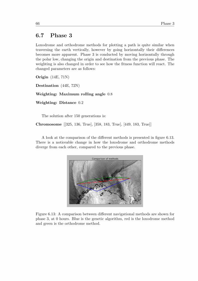
66 Phase 3
6.7 Phase 3
Loxodrome and orthodrome methods for plotting a path is quite similar whentraversing the earth vertically, however by going horizontally their differencesbecomes more apparent. Phase 3 is conducted by moving horizontally throughthe polar low, changing the origin and destination from the previous phase. Theweighting is also changed in order to see how the fitness function will react. Thechanged parameters are as follows:
Origin (14E, 71N)
Destination (44E, 72N)
Weighting: Maximum rolling angle 0.8
Weighting: Distance 0.2
The solution after 150 generations is:
Chromosome [[325, 136, True], [358, 183, True], [449, 183, True]]
A look at the comparison of the different methods is presented in figure 6.13.There is a noticeable change in how the loxodrome and orthodrome methodsdiverge from each other, compared to the previous phase.
Figure 6.13: A comparison between different navigational methods are shown forphase 3, at 0 hours. Blue is the genetic algorithm, red is the loxodrome methodand green is the orthodrome method.
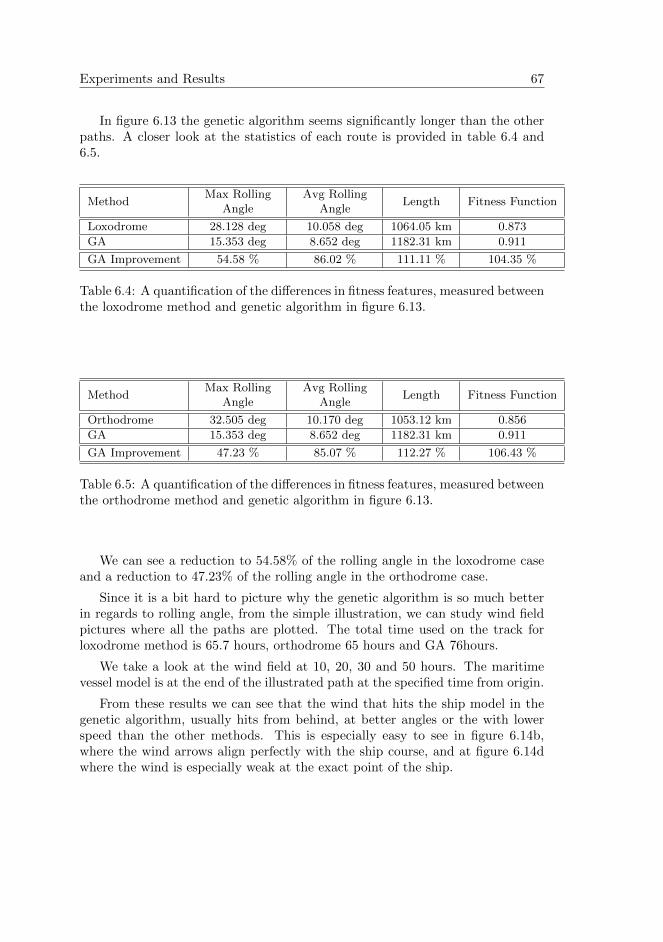
Experiments and Results 67
In figure 6.13 the genetic algorithm seems significantly longer than the otherpaths. A closer look at the statistics of each route is provided in table 6.4 and6.5.
MethodMax Rolling
AngleAvg Rolling
AngleLength Fitness Function
Loxodrome 28.128 deg 10.058 deg 1064.05 km 0.873
GA 15.353 deg 8.652 deg 1182.31 km 0.911
GA Improvement 54.58 % 86.02 % 111.11 % 104.35 %
Table 6.4: A quantification of the differences in fitness features, measured betweenthe loxodrome method and genetic algorithm in figure 6.13.
MethodMax Rolling
AngleAvg Rolling
AngleLength Fitness Function
Orthodrome 32.505 deg 10.170 deg 1053.12 km 0.856
GA 15.353 deg 8.652 deg 1182.31 km 0.911
GA Improvement 47.23 % 85.07 % 112.27 % 106.43 %
Table 6.5: A quantification of the differences in fitness features, measured betweenthe orthodrome method and genetic algorithm in figure 6.13.
We can see a reduction to 54.58% of the rolling angle in the loxodrome caseand a reduction to 47.23% of the rolling angle in the orthodrome case.
Since it is a bit hard to picture why the genetic algorithm is so much betterin regards to rolling angle, from the simple illustration, we can study wind fieldpictures where all the paths are plotted. The total time used on the track forloxodrome method is 65.7 hours, orthodrome 65 hours and GA 76hours.
We take a look at the wind field at 10, 20, 30 and 50 hours. The maritimevessel model is at the end of the illustrated path at the specified time from origin.
From these results we can see that the wind that hits the ship model in thegenetic algorithm, usually hits from behind, at better angles or the with lowerspeed than the other methods. This is especially easy to see in figure 6.14b,where the wind arrows align perfectly with the ship course, and at figure 6.14dwhere the wind is especially weak at the exact point of the ship.
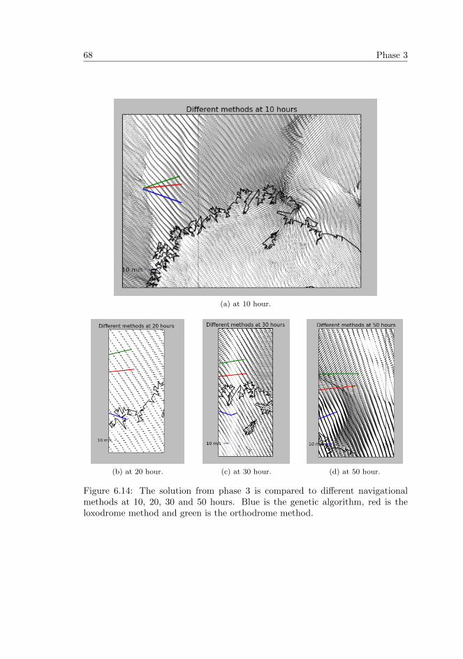
68 Phase 3
(a) at 10 hour.
(b) at 20 hour. (c) at 30 hour. (d) at 50 hour.
Figure 6.14: The solution from phase 3 is compared to different navigationalmethods at 10, 20, 30 and 50 hours. Blue is the genetic algorithm, red is theloxodrome method and green is the orthodrome method.
Experiments and Results 69
6.8 Phase 4
Previous results show that the algorithm will usually avoid the polar low, whengiven the chance. A particularly interesting application of the algorithm is howit will navigate inside of a polar low, or rather navigate out of it.
The following scenario is constructed so that the ship model starts in thepolar low at time 0 and has to navigate out of the polar low towards Tromsø atdestination (69,40N 18,56E).
This scenario presents a particularly dangerous environments for small mar-itime vessels. The weighting of maximum rolling angle will be set to very highand the weighting of distance to very low, yielding the following parameters:
Generations 150
Population 20
Weight: Max rolling angle 0.95
Weight: Distance 0.05
origin (38E, 72N)
destination (18.6E, 69.4N)
The resulting path was found:
Chromosome [[393, 166, True], [309, 166, True], [315, 211, True], [338, 199,True], [356, 213, True], [355, 185, True], [359, 184, True], [351, 154, True],[329, 166, True]]
At first glance this solution does not seem optimal. It passes quite close tothe destination and then proceeds to make a big loop before finishing at thedestination. This can be due to several factors, for instance insufficient evolutionfor the solution, the extreme weighting of the max rolling angle feature or acombination of both.
If we take a closer look at the point where the path is close to the destinationit might shed some light on the choice of taking a loop. Figure 6.16 shows thepath at 31 hours from origin. The final destination is highlighted.
Stopping the algorithm path at 31 hours and going straight to the destinationmarker seems like a reasonable choice for the algorithm. The coordinate at 31hours is (19.2476 E, 69.4274 N) which translates to (331, 169) in grid coordinates.A modified path is constructed by stopping the solution path at 31 hours andthen drawing a straight line to the destination. The real world coordinate at 31hours is calculated to grid coordinates and substitutes the second node in theoriginal solution, resulting in the following chromosome path:
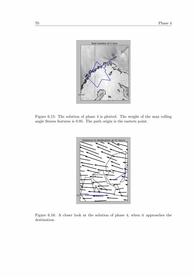
70 Phase 4
Figure 6.15: The solution of phase 4 is plotted. The weight of the max rollingangle fitness features is 0.95. The path origin is the eastern point.
Figure 6.16: A closer look at the solution of phase 4, when it approaches thedestination.
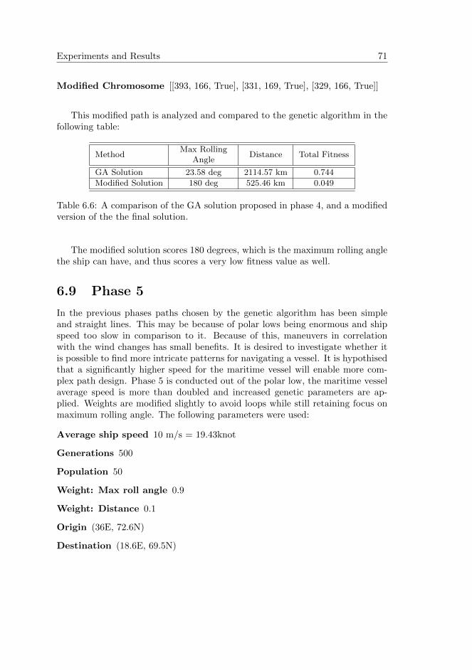
Experiments and Results 71
Modified Chromosome [[393, 166, True], [331, 169, True], [329, 166, True]]
This modified path is analyzed and compared to the genetic algorithm in thefollowing table:
MethodMax Rolling
AngleDistance Total Fitness
GA Solution 23.58 deg 2114.57 km 0.744
Modified Solution 180 deg 525.46 km 0.049
Table 6.6: A comparison of the GA solution proposed in phase 4, and a modifiedversion of the the final solution.
The modified solution scores 180 degrees, which is the maximum rolling anglethe ship can have, and thus scores a very low fitness value as well.
6.9 Phase 5
In the previous phases paths chosen by the genetic algorithm has been simpleand straight lines. This may be because of polar lows being enormous and shipspeed too slow in comparison to it. Because of this, maneuvers in correlationwith the wind changes has small benefits. It is desired to investigate whether itis possible to find more intricate patterns for navigating a vessel. It is hypothisedthat a significantly higher speed for the maritime vessel will enable more com-plex path design. Phase 5 is conducted out of the polar low, the maritime vesselaverage speed is more than doubled and increased genetic parameters are ap-plied. Weights are modified slightly to avoid loops while still retaining focus onmaximum rolling angle. The following parameters were used:
Average ship speed 10 m/s = 19.43knot
Generations 500
Population 50
Weight: Max roll angle 0.9
Weight: Distance 0.1
Origin (36E, 72.6N)
Destination (18.6E, 69.5N)
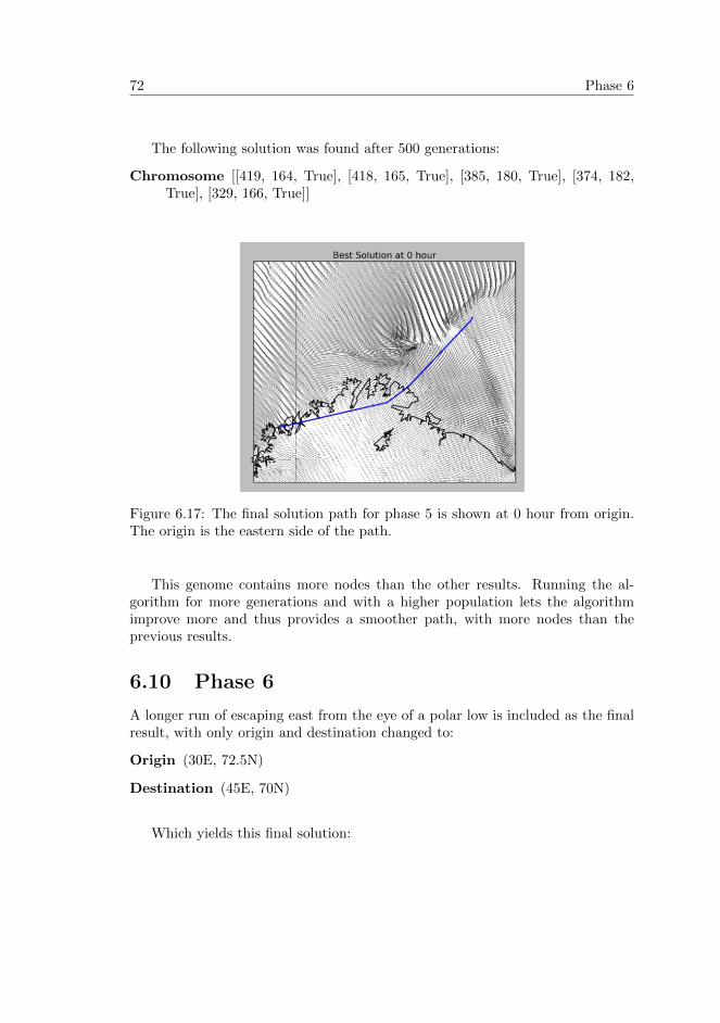
72 Phase 6
The following solution was found after 500 generations:
Chromosome [[419, 164, True], [418, 165, True], [385, 180, True], [374, 182,True], [329, 166, True]]
Figure 6.17: The final solution path for phase 5 is shown at 0 hour from origin.The origin is the eastern side of the path.
This genome contains more nodes than the other results. Running the al-gorithm for more generations and with a higher population lets the algorithmimprove more and thus provides a smoother path, with more nodes than theprevious results.
6.10 Phase 6
A longer run of escaping east from the eye of a polar low is included as the finalresult, with only origin and destination changed to:
Origin (30E, 72.5N)
Destination (45E, 70N)
Which yields this final solution:
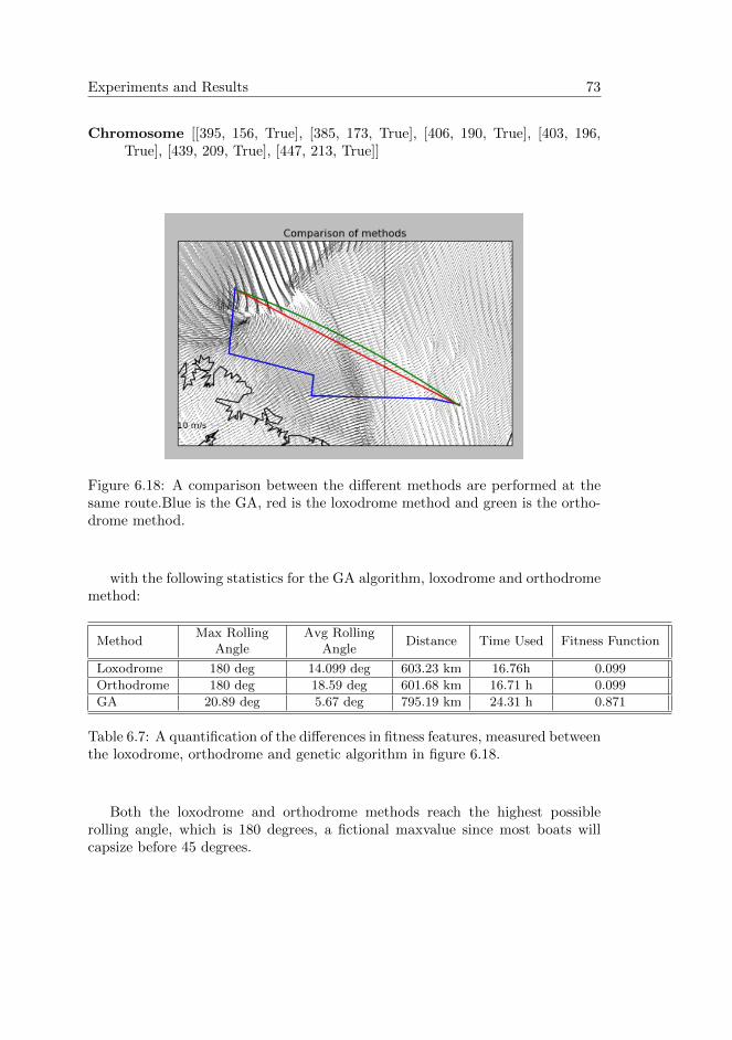
Experiments and Results 73
Chromosome [[395, 156, True], [385, 173, True], [406, 190, True], [403, 196,True], [439, 209, True], [447, 213, True]]
Figure 6.18: A comparison between the different methods are performed at thesame route.Blue is the GA, red is the loxodrome method and green is the ortho-drome method.
with the following statistics for the GA algorithm, loxodrome and orthodromemethod:
MethodMax Rolling
AngleAvg Rolling
AngleDistance Time Used Fitness Function
Loxodrome 180 deg 14.099 deg 603.23 km 16.76h 0.099
Orthodrome 180 deg 18.59 deg 601.68 km 16.71 h 0.099
GA 20.89 deg 5.67 deg 795.19 km 24.31 h 0.871
Table 6.7: A quantification of the differences in fitness features, measured betweenthe loxodrome, orthodrome and genetic algorithm in figure 6.18.
Both the loxodrome and orthodrome methods reach the highest possiblerolling angle, which is 180 degrees, a fictional maxvalue since most boats willcapsize before 45 degrees.
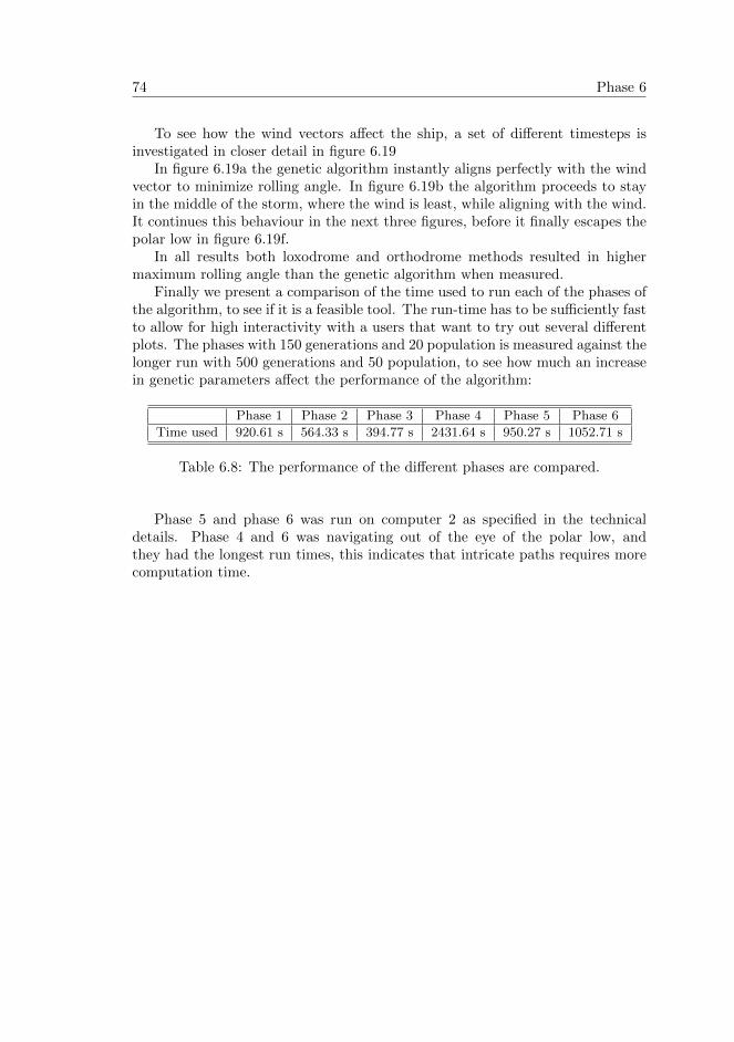
74 Phase 6
To see how the wind vectors affect the ship, a set of different timesteps isinvestigated in closer detail in figure 6.19
In figure 6.19a the genetic algorithm instantly aligns perfectly with the windvector to minimize rolling angle. In figure 6.19b the algorithm proceeds to stayin the middle of the storm, where the wind is least, while aligning with the wind.It continues this behaviour in the next three figures, before it finally escapes thepolar low in figure 6.19f.
In all results both loxodrome and orthodrome methods resulted in highermaximum rolling angle than the genetic algorithm when measured.
Finally we present a comparison of the time used to run each of the phases ofthe algorithm, to see if it is a feasible tool. The run-time has to be sufficiently fastto allow for high interactivity with a users that want to try out several differentplots. The phases with 150 generations and 20 population is measured against thelonger run with 500 generations and 50 population, to see how much an increasein genetic parameters affect the performance of the algorithm:
Phase 1 Phase 2 Phase 3 Phase 4 Phase 5 Phase 6
Time used 920.61 s 564.33 s 394.77 s 2431.64 s 950.27 s 1052.71 s
Table 6.8: The performance of the different phases are compared.
Phase 5 and phase 6 was run on computer 2 as specified in the technicaldetails. Phase 4 and 6 was navigating out of the eye of the polar low, andthey had the longest run times, this indicates that intricate paths requires morecomputation time.
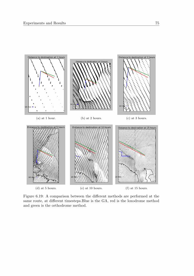
Experiments and Results 75
(a) at 1 hour. (b) at 2 hours. (c) at 3 hours.
(d) at 5 hours. (e) at 10 hours. (f) at 15 hours.
Figure 6.19: A comparison between the different methods are performed at thesame route, at different timesteps.Blue is the GA, red is the loxodrome methodand green is the orthodrome method.

76 Phase 6
Chapter 7
Discussion and Evaluation
To justify the results of a project there is a need to evaluate the findings andmethods used. How a project is evaluated is dependent on the nature of theproject. The author attempts to answer the research questions and discuss theresults found in the previous chapters. Finally thorough evaluation is conductedin accordance to the criterias listed in Cohen and Howe [1988].
7.1 Research Questions
Each of the research questions defined is listed with a discussion on how theywere addressed.
Research question 1 Can a genetic algorithm find an optimal path in a mar-itime environment ?
This research questions was constructed to figure out if it is possible to use thegenetic algorithm method a maritime environment. Phase 1 carefully investigatesthe genetic algorithm process in the maritime environment and shows how it ispossible for a genetic algorithm to approach an optimal path.
Research Question 2 How will the genetic algorithm compare to more tradi-tional methods of path-planning?
Research question 2 was designed to compare the genetic algorithm to othermethods that exists for navigating in maritime environment. The loxodrome andorthodrome methods were selected and defined in chapter 3. In phase 2,3 and
78 Discussion
6 the genetic algorithm solution is compared to the loxodrome and orthodromemethods. The fitness features of the different methods are carefully analyzed,revealing that genetic algorithm can improve greatly upon the maximum rollingangle for a path, and as a result the safety of the maritime vessel.
Research Question 3 How will the genetic algorithm handle particularly inter-esting applications, such as navigating through a polar low, and navigatingout of a polar low?
The main focus of the genetic algorithm is how wind forces act on a maritimevessel and how this affects safety of the vessel. Safety concerning the vessel isdiscussed in chapter 3. The theory section highlights that high speed and rapidchanging winds is one of the greatest threats to safety of a vessel. Polar lowscontain these both these hazards. Navigation around, through and out of a polarlow is investigate in phase 1 through 6, in chapter 6.
7.2 Discussion
The findings are commented to a certain extent in chapter 6. In this section theresearch questions are answered and then interesting aspects of the algorithm arediscussed.
7.2.1 Rolling Angles
The genetic algorithm can effectively reduce maximum rolling angle and averagerolling angle of a maritime vessel for a given route. Table 6.2 and 6.3 in phase2 shows that the genetic algorithm can reduce maximum rolling angle to 38.56%of loxodrome and 31.91% of orthodrome method. Table 6.4 and 6.5 in phase3 shows that the genetic algorithm can reduce maximum rolling angle of loxo-drome and orthodrome methods to 54.58% and 47.23% respectively, in high windareas. Overall it was shown that the genetic algorithm can reduce the maximumrolling angle in comparison to loxodrome and orthodrome methods, which is animportant factor for increasing the safety of maritime vessels.
7.2.2 Phase 4
In phase 4, figure 6.15, the final solution appears suboptimal. The final pathpasses the destination and proceeds to take a loop, before going towards thedestination. A possible reason for this unexpected choice of path is the extremeweighting of maximum rolling angle used in the experiment. Another possible
Discussion and Evaluation 79
reason is limitations in precision. The algorithm can only take on geographicalvalues described in the wind data file, which is an unwanted limitation. Thechoice of this type of limitation has been discussed, and was chosen because ofa need for discretizing the search space. However, increasing the precision andpossible values the algorithm can take on is an important point to improve inpotential further work.
7.2.3 Selection Mechanisms
In late generations the fitness values are very similar(see figure 6.12) with smallchanges between the best solutions. Similar fitness values in combination withroulette-wheel selection causes the selection probability of all individuals to besimilar. This means that the best solution has approximately the same chance ofbeing chosen for reproduction as the close to best solution. This is low selectionpressure and is undesirable, since we want the very best individuals to reproduce.Introducing tournament selection later stages of the generations could help solvethe low selection pressure. Tournament selection chooses a group of individualsfrom the population and rank them within the group. The individuals are thengiven selection probability in correlation with their ranking within the group.Using a combination of these selection mechanisms could increase the selectionpressure at all stages throughout the algorithm.
7.2.4 Reproducibility of Experiments
The random nature of the operations done in the algorithm on path solutions,makes it highly unlikely to reproduce the exact same result on two separatealgorithm runs. However, running the algorithm with similar parameters, shouldresult in somewhat similar results when they approach an optimal solution. Thenature of genetic algorithm states that it has no guarantee of getting an optimalsolution, so two different runs does not guarantee the same results. It should stillbe possible to analyse the results and compare them more traditional methodsto determine the benefits of this system.
7.2.5 Performance
It is difficult to conclude anything from the time used for each run of the al-gorithm, shown in table 6.8. They were run on 2 different systems, where thesystem setup used for phase 5 and 6 were on a dedicated machine and used forthe higher genetic parameter runs. The longer runs in phase 5 and 6 performedat similar speed as the rest of the experiments even though they had significantlyhigher genetic parameters. The time for each run of the algorithm is a bit highfor enabling high interaction with a user. Possible ways to improve performance
80 Limitations
is through using dedicated machines, faster systems or improve the algorithmefficiency through algorithm analysis.
7.2.6 Utility of the algorithm
As we can see from the performance of the different phases, the algorithm requiresquite some time and computational power to produce good results.Since manyboats are old, with old hardware and minimal computing power, it is not feasibleto run the algorithm on-board the ship. To let these users be able to benefitfrom the algorithm, it should be accessible through an online service, e.g. theBarentswatch portal. The user would input their preferences, and the all thecomputations related to the algorithm would be performed on the server side.The user would then be presented with their results when a criteria is met, e.g.a given time has elapsed, or a sufficiently good solution has been found. Thisallows users to benefit from the algorithm without the need for any computationon their side, they would only need a browser and a connection to the internet.
7.3 Limitations
In this section limitations to the algorithm is highlighted and discussed.
7.3.1 Wind Data
The wind data, and uncertainties of it, is one of the main limitations to thethesis. The algorithm needs as precise wind data, and high resolution, as possible.However, if the data has too high resolution and time steps are increased thealgorithm performance will suffer greatly. This will result in slow performanceand inability to provide fast navigational guidance, as intended. If the wind datacan be simplified without losing precision and resolution the performance andquality of the algorithm will increase.
7.3.2 Terrain
Terrain was implemented as feasible and unfeasible grids in the genetic algorithmimplementation, but all terrain was disregarded in results. The terrain was dis-regarded because the polar low was on top of terrain in the wind data, and themost interesting results were connected to navigation around and through a po-lar low. Another reason was lack of sufficiently good quality terrain data. Thismeans that shallow water is disregarded as well.
Discussion and Evaluation 81
7.3.3 Blendermann Method Limitations
The tests are performed in a wind tunnel scenario, and the method relies heavilyon empirical data. When maritime vessels are observed in their natural en-vironment, additional factors arise. For instance the effects of wind gradient,turbulence, efficiency of wind shelter and how wind affects a heavy tilted ship.Blendermann [1994] notes that in these cases the wind loading functions does notchange, but wind load parameter values must adjusted.
7.3.4 Average Speed
To calculate the exact speed of a maritime vessel is not a trivial task. Speed isaffected by wind, waves and currents, and these are subject to rapid changes.For simplification the average speed used is a static value, provided by the motorcapabilities. In reality the speed of a maritime vessel will vary depending on theweather conditions, load on the vessel and navigation decisions.
Another limitation of having a constant average speed is that it makes itimpossible to find some paths. The most intelligent solution to a problem couldfor instance consist of staying at one location until the wind blows over, and thenmove. Constant average speed also makes it impossible to navigational patternsthat move at different speeds through areas, which could decrease wind forces onthe vessel.
7.3.5 Traffic
That there are no crossing ship trajectories. If the path cross another vessel’strajectory the captain is expected to handle the necessary avoidance maneuver.The difference in path caused by such a maneuver is assumed to be negligible.
7.3.6 Weights
The algorithm could also be designed to find the pareto optimal front for anorigin and destination, and then let the user select the most appropriate routefrom this set of solutions. Using the pareto-optimal front could be a usefulalternative approach to the algorithm. This would require the algorithm to knowthe origin and destination beforehand.
7.3.7 Time Domain
The wind is measured at every whole hour. Any changes to the weather happen-ing between the full hours is not registered.Finding the wind data between everyhour is not easily dealt with, since it is very resource demanding to accumulate
82 Limitations
and work with wind data that is delivered at a smaller intervals. Weather canchange quite drastically within an hour, so this is a weakness in the wind data.One way to deal with this is to approximate the intermediary wind values as afunction of the wind data at every whole hour, however this representation ofwind data would not sufficiently precise.
7.3.8 Format
The wind data has to be specified as a netCDF file, this is a standard used for mostscientific data, especially weather forecasting data. The maritime vessel modelhas no standard file input. When making a new ship model for the algorithmevery value that is used has to be inputted into the ship model class, which canbe tedious. This can be solved by developing a standard for specifying maritimevessel models and an easy and intuitive way of input them.
7.3.9 On Board Sensors
A way to improve predictions of weather, advanced sensors can measure realtime data more precise and compare them to the weather predictions to helpthe algorithm make better decisions. The genetic algorithm can work as a toolto complement the captains observations and experience, to make better deci-sions for navigation. Together, the genetic algorithm and the captains expertknowledge can make an even better path.
7.3.10 Scalability
At present when doing simulations the system performs at a decent rate. Whenincreasing the resolution of the wind data and grid resolution, the algorithm willhave to be run for more generations to develop a sufficiently good path. Com-putations will take longer because the chromosomes will be longer to deal withthe increased resolution. This will cause a scalability issue where the algorithmwill perform slower than it is doing at the moment. This could pose a problemfor further work on the system. Improving upon the algorithm and running on adedicated and faster setup is a necessary step towards addressing this problem.
7.3.11 Safety Hazard of Icing on Ships
An aspect that was investigated in regards to the design of the algorithm is icingon ships, and the safety hazards that this presents. IMO A749(18) reveals thatto be able to measure the risk of icing and determining the dangerous areas alonga route requires knowledge of temperature along this path as well, which was not
Discussion and Evaluation 83
available for this study. However, icing is a very important aspect of safety formaritime vessels and should be looked into for further work.
Ice formation adversely affects the seaworthiness of the vessel as ice formationleads to:
1. An increase in the weight of the vessel due to accumulation of ice on thevessel’s surface. This causes a reduction in freeboard and buoyancy.
2. A rise of the vessel’s centre of gravity due to high location of ice on thevessel’s structures. This causes corresponding reduction in the level ofstability.
3. An increase of windage area due to ice formation on the upper parts of thevessel and hence an increase in heeling moment due to the action of thewind.
4. A change of trim due to uneven distribution of ice along the vessel’s length.Trim is when a ship is tilting forward or backwards.
5. The development of a constant list due to uneven distribution of ice acrossthe breadth of the vessel. List is similar to trim, it acts on the sides of theship, so list is when a ship is tilting to one of the sides due to added weight.
6. Impairment of the maneuverability and reduction of the speed of the vessel.
The main points gathered from IMO A749(18) were meteorological conditionscausing the most comomon type of ice formation due to spraying of the vessel,where spraying is water transported to the vessel by wind. Slow accumulation ofice takes place when:
1. at ambient temperature from -1 celsius to -3 celsius and any wind force
2. at ambient temperature from -4 celsius and lower and wind force from 0 to9 m/s
Very fast accumulation of ice takes place:
1. at ambient temperature of -4 celsius and lower and wind forces of 16m/sand over
2. at ambient temperature of -9 celsius and lower and wind force 10 to 15 m/s
84 Further Work
7.4 Further Work
As this system is a first prototype, a part of the thesis objective has been to givean extensive overview over the intricacies and challenges presented in this projectand suggestions for further work.
7.4.1 Higher Resolution Grid
Using wind data grid as the only viable positions that the maritime vessel canmove between is restricting. Allowing the algorithm to take on more locationswill allow for smoother movement and more complex movement patterns, butwould also require significantly more computation power.
7.4.2 Terrain
To complement the increased resolution grid for movement and wind, a suffi-ciently high resolution terrain data should be included. This will allow the algo-rithm to find paths that can maneuver in low waters depending on the depth ofthe ship, instead of just out at the deep sea.
7.4.3 Plotting
In chapter 6 the figures are plotted using matplotlib. These figures had to bemanually configured for every result to allow for decent illustrations of path andwind plotting.
When the plot is fully zoomed out the windquivers should be sufficiently small,so they don’t clutter and block the contours of terrain that lies under them. Atthe same time they have to be sufficiently large so it is possible to see where thereare strong winds and where the wind creates specific patterns, such as polar lows.On the other hand when zooming in the quivers should expand to get thicker soit is possible to see each individual wind quiver and study the data in greaterdetail.
This plotting function is a very delicate tuning process of visualization andzoom parameters, and automatization of this fine calibration was not a focus ofthe thesis. For further work, a clear improvement for ease of use and intuitivenessof the system would be to automate the visualization process. This would includealways providing good plots that give a clear view of all relevant aspects of thesolution.
Discussion and Evaluation 85
7.4.4 Redundancy
Towards the end of the algorithm, a lot of identical paths are evaluated, whichcauses unnecessary work. For these cases a lookup table could be created duringthe algorithm, which stored the values for the most popular solutions, so theywouldn’t have to be recalculated every time an already visited path was mutatedinto. Finding identical solutions in a lookup table, or similar solutions could savea lot of computation time, since most of the computation of the algorithm goesinto computing the fitness and wind moments on a ship.
7.4.5 Evolve Time for Each Node
Earlier alternating speed for a ship was discussed. A solution to include alter-nating speed in the algorithm is to evolve time used for each segment of thepath. Some limitations to how fast a passage could be traversed would have tobe computed from the ship model.
This extra implementation would include the additional element of alternat-ing speed, which could be an interesting aspect for the system, instead of theconstant average speed of the maritime vessel, which is used in this implementa-tion. Including alternating speed could introduce more complex calculations offuel usage, time usage and speed of the path, and could give suggestions of whenit is safe to give full speed and when the vessel should move slower or even stop.
7.4.6 Risk Curve
Punishing the rolling angle of a maritime vessel linearly from 0 to 90 degrees isunlikely the best solution. A vessel can have quite high rolling angles dependingon ship characteristics, up to a certain point, without any threat to safety. Mostships can roll towards 30 degrees without danger, depending on their hull andvessel characteristics. Instead of using linear punishment of the rolling angles, afitted sinus curve could be a better approximation. The sinus curve would threatlow angles ranging from 0 to 10 with very low threat to safety, then punish angleshigher than 10 degrees increasingly more.
7.4.7 Performance
A common nominator in the further work area is to increase performance, makethe algorithm faster, get higher resolution and smoother movement for small scalenavigation. A faster system can be achieved by changing to a faster programminglanguage to control the system in more detail. The algorithm can be specializedfor the system platform and more careful control of resources can optimize the
86 Threats to Validity
performance of the algorithm. A faster system would allow for more and fastercomputations, which would allow for better user interaction as well.
7.5 Threats to Validity
Threats to validity are aspects with the results that can make them hard toreproduce or cause the results to not be valid.
7.5.1 Time
If time exceeds the time that there is recorded wind data for they will simplyuse the latest wind data that exists. These wind data will not be correct, andis a threat to validity. However, since this only occours at exceptionally longsolutions these solutions will usually not be included in any final solution set,because they have too long distance.
7.5.2 Algorithm Performance
Time measurements done for the algorithms were performed on laptops withseveral other running applications and different work-loads at different times.Looking at the run-time of the algorithm at different phases they are very spread.For more precise performance calculations the algorithm should have been runin a dedicated environment.
7.5.3 Diversity
The algorithm was only tested on one type of wind data and one type of shipmodel, which may introduce bias. Further work should include extensive testingwith different ship models and wind data, to verify the value of the program.
7.6 Evaluation
The model presented in Cohen and Howe [1988] is used to justify the choice ofproject and has served as a guidance throughout structuring and conducting thethesis. The model consists of five steps:
1. refine the topic to a task
2. design the method
3. build a program
Discussion and Evaluation 87
4. design experiments
5. analyze the experiments and results
The five steps will be summarized in the following sections:
7.6.1 Refine the Topic to a Task
To refine the problem, a set of research questions was defined. Previous def-initions of the problem and how they were handled is discussed in chapter 2,the most relevant one being MEWRA. The differences between these methods ishighlighted and a justification for creating a new algorithm consisting of arcticwind data and using a representative ship model for this region is argumentedfor. The task is simplified by abstracting away some aspects listed in the scope.
7.6.2 Design the Method
The second step naturally relies on the first step, and addresses the research ques-tions with the necessary theory and methods found in chapter 2 . Argumentationsfor methods are provided.
7.6.3 Build a Program
A detailed implementation of the genetic algorithm is provided in chapter 4.This describes how the solutions are produced and how they are represented.This section also discusses any unforeseen problems encountered and how thesewere handled.
7.6.4 Design Experiments
A detailed experiment setup and plan is provided in the beginning of chapter 6.These experiments are performed to demonstrate how well the program works.The experiments are designed to be compared against traditional navigationmethods, and validity of these experiments rely on identical conditions for allmethods, which is provided.
7.6.5 Analyze the Experiments and Results
The experiment results are shown in chapter 6. The results includes all thedifferent phases and scenarios from the experiments plan. The results are showntogether with comments meant to guide the reader through the experiments.Further in this chapter, the results are discussed, comparisons are made to other

88 Evaluation
methods and limitations of the program is highlighted. Finally, the performanceof the program is considered.
Chapter 8
Conclusion
The main goal for this thesis has been to implement a path planning systemfor maritime navigation in arctic regions. The author has implemented a fullyfunctional genetic algorithm that processes wind data in the arctic region, andcreates an optimal path given user input.
The system is highly modular and highly configurable, which allows the userto specify which parameters he wishes to focus on, in relation to wind effects onmaritime vessels.
Execution of extensive simulation runs in the arctic region shows that thesystem can find paths that are hard to discover by using traditional methods ofpathplanning, due to the added dimension of time-domain simulation and windforces on the maritime vessel.
Besides the delivered system, a list of potential improvements and limita-tions of the algorithm has been discussed, which may be implemented in futureprojects.
8.1 Generalization
By substituting the ship model with a model of any vessel, the problem can begeneralized as reducing side-force moment on any type of vessel, and could beused in any vessel problem that seeks to minimize length of a path and side-forcemoment on their vessel.

90 Contributions To The Research Field
8.2 Contributions To The Research Field
The author’s previous specialization project uncovered that using artificial in-telligence methods in combination with maritime path-planning is a relativelyuntested area of path-planning. Most of the literature is focused on autonomouscollision-avoidance, cargo optimization and traffic optimization.
In light of the results found in this thesis, the genetic algorithm has been suc-cessfully applied as a multi-objective evolutionary algorithm for weather routeingin extreme weather for the arctic regions.
Bibliography
Alvarez, A., Caiti, A., and Onken, R. (2004). Evolutionary path planning forautonomous underwater vehicles in a variable ocean. Oceanic Engineering,IEEE Journal of, 29(2):418–429.
Barraquand, J., Langlois, B., and Latombe, J.-C. (1991). Numerical potentialfield techniques for robot path planning. In Advanced Robotics, 1991. ’Robotsin Unstructured Environments’, 91 ICAR., Fifth International Conference on,pages 1012–1017 vol.2.
Blendermann, W. (1994). Parameter identification of wind loads on ships. Journalof Wind Engineering and Industrial Aerodynamics, 51(3):339–351.
Chen, D., Szczerba, R., and Uhran, J. J. (1995). Planning conditional shortestpaths through an unknown environment: a framed-quadtree approach. InIntelligent Robots and Systems 95. ’Human Robot Interaction and CooperativeRobots’, Proceedings. 1995 IEEE/RSJ International Conference on, volume 3,pages 33–38 vol.3.
Cohen, P. R. and Howe, A. E. (1988). How evaluation guides ai research: Themessage still counts more than the medium. AI Magazine, 9(4):35.
Dubrovsky, O., Levitin, G., and Penn, M. (2002). A genetic algorithm with acompact solution encoding for the container ship stowage problem. Journal ofHeuristics, 8(6):585–599.
Fiskeridirektoratet (2014). Norwegian fishing vessels fishermen and licenses 2013.Technical report, Fiskeridirektoratet.
Floreano, D. and Mattiussi, C. (2008). Bio-inspired artificial intelligence: theo-ries, methods, and technologies. MIT press.
Fossen, T. I. (2011). Handbook of marine craft hydrodynamics and motion control.John Wiley & Sons.
92 Bibliography
Garau, B., Alvarez, A., and Oliver, G. (2005). Path planning of autonomousunderwater vehicles in current fields with complex spatial variability: an a*approach. In Robotics and Automation, 2005. ICRA 2005. Proceedings of the2005 IEEE International Conference on, pages 194–198.
Holland, J. H. (1975). Adaption in natural and artificial systems.
Hollnagel, E. (1996). Reliability analysis and operator modelling. ReliabilityEngineering and System Safety, 52(3):327–337.
Hornby, G. S., Globus, A., Linden, D. S., and Lohn, J. D. (2006). Automatedantenna design with evolutionary algorithms. In AIAA Space, pages 19–21.
Hromkovic, J. (2010). Algorithmics for hard problems: introduction to combina-torial optimization, randomization, approximation, and heuristics. Springer-Verlag.
Ito, M., Zhnng, F., and Yoshida, N. (1999). Collision avoidance control of shipwith genetic algorithm. In Control Applications, 1999. Proceedings of the 1999IEEE International Conference on, volume 2, pages 1791–1796 vol. 2.
James, R. W. (1957). Application of wave forecasts to marine navigation.
Janikow, C. Z. and Michalewicz, Z. (1991). An experimental comparison of binaryand floating point representations in genetic algorithms. In ICGA, pages 31–36.
Jarvis, R. (2006). Robot path planning: complexity, flexibility and applicationscope. In Proceedings of the 2006 international symposium on Practical cogni-tive agents and robots, pages 3–14. ACM.
Kamon, I. and Rivlin, E. (1995). Sensory based motion planning with globalproofs. In Intelligent Robots and Systems 95. ’Human Robot Interaction andCooperative Robots’, Proceedings. 1995 IEEE/RSJ International Conferenceon, volume 2, pages 435–440 vol.2.
Kobayashi, E., Asajima, T., and Sueyoshi, N. (2011). Advanced navigation routeoptimization for an oceangoing vessel. TransNav, the International Journal onMarine Navigation and Safety of Sea Transportation, 5(3):377–383.
Kobylinski, L. (2007). System and risk approach to ship safety, with special em-phasis of stability. Archives of Civil and Mechanical Engineering, 7(4):97–106.
Krata, P. (2008). Total losses of fishing vessels due to the insufficient stability.TransNav, the International Journal on Marine Navigation and Safety of SeaTransportation, 2(3):311–315.
Bibliography 93
Kwon, K.-Y., Cho, J., Yoo, B.-S., and Joh, J. (2005). Autonomous navigationof an underwater robot using fuzzy logic. In Fuzzy Information ProcessingSociety, 2005. NAFIPS 2005. Annual Meeting of the North American, pages540–545. IEEE.
Lacki, M. (2008). Reinforcement learning in ship handling. TransNav, the In-ternational Journal on Marine Navigation and Safety of Sea Transportation,2(2):157–160.
Manley, J. (2008). Unmanned surface vehicles, 15 years of development. InOCEANS 2008, pages 1–4.
Norrbin, N. H. (1971). Theory and observations on the use of a mathematicalmodel for ship manoeuvring in deep and confined waters. Technical report,DTIC Document.
Petkovi, D. (2011). Dynamic programming algorithm vs. genetic algorithm:Which is faster? In Bramer, M., Petridis, M., and Hopgood, A., editors, Re-search and Development in Intelligent Systems XXVII, pages 483–488. SpringerLondon.
Rasmussen, E. (1979). The polar low as an extratropical cisk disturbance. Quar-terly Journal of the Royal Meteorological Society, 105(445):531–549.
Rechenberg, I. (1965). Cybernetic solution path of an experimental problem.
Roberge, V., Tarbouchi, M., and Labonte, G. (2013). Comparison of paral-lel genetic algorithm and particle swarm optimization for real-time uav pathplanning. Industrial Informatics, IEEE Transactions on, 9(1):132–141.
Sinnott, R. W. (1984). Virtues of the haversine. Sky and telescope, 68:158.
Smierzchalski, R. (1999). Evolutionary trajectory planning of ships in navigationtraffic areas. Journal of Marine Science and Technology, 4(1):1–6.
Szlapczynska, J. and Smierzchalski, R. (2009). Multicriteria optimisation inweather routing. TransNav, the International Journal on Marine Navigationand Safety of Sea Transportation, 3(4):393–400.
Vasudevan, C. and Ganesan, K. (1996). Case-based path planning for au-tonomous underwater vehicles. Autonomous Robots, 3(2-3):79–89.
Weise, T. (2009). Global optimization algorithms–theory and application. Self-Published,.
Zheng, C., Li, L., Xu, F., Sun, F., and Ding, M. (2005). Evolutionary route plan-ner for unmanned air vehicles. Robotics, IEEE Transactions on, 21(4):609–620.

94 Bibliography
Appendix A: Ship model
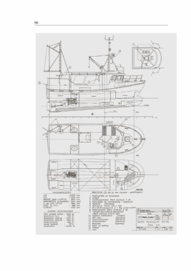
96
Related Documents