AMPLITUDE SCINTILLATIONS ON EARTH-SPACE PROPAGATION PATHS AT 2 AND 30 GHz D. N. J. Devasirvatham and D. B. Hodge (NASA-CR-156785) AMPLTUDE SCINTIlIALTIO1S ON EARTH-SPACE PROPAGATION PAT-HS AT 2 AND 30 GHz M.S. Thesis (Ohio State Univ., columbus.) 101 p HC A06/PF A01 CSCL 20N G3/32 The Ohio State University ElectroScience Laboratory Department of Electrical Engineering Columbus, Ohio 43212 Technical Report 4299-4 March 1977 Prepared for National Aeronautics and Space Administration GODDARD SPACE FLIGHT CENTER Greenbelt, Maryland 20771 IN7-293,q% - -' Unclas 28378 A UG 1978 #L"4 https://ntrs.nasa.gov/search.jsp?R=19780021364 2020-03-22T03:35:24+00:00Z

Welcome message from author
This document is posted to help you gain knowledge. Please leave a comment to let me know what you think about it! Share it to your friends and learn new things together.
Transcript
AMPLITUDE SCINTILLATIONS ON EARTH-SPACE PROPAGATION PATHS AT 2 AND 30 GHz
D N J Devasirvatham and D B Hodge
(NASA-CR-156785) AMPLTUDE SCINTIlIALTIO1S ON EARTH-SPACE PROPAGATION PAT-HS AT 2 AND 30
GHz MS Thesis (Ohio State Univ columbus) 101 p HC A06PF A01 CSCL 20N
G332
The Ohio State University
ElectroScience Laboratory Department of Electrical Engineering
Columbus Ohio 43212
Technical Report 4299-4
March 1977
Prepared for National Aeronautics and Space Administration
GODDARD SPACE FLIGHT CENTER Greenbelt Maryland 20771
IN7-293q - -
Unclas 28378
A UG 1978
L4
httpsntrsnasagovsearchjspR=19780021364 2020-03-22T033524+0000Z
NOTICES
When Government drawings specifications or other data are used for any purpose other than in connection with a definitely related Government procurement operation the United States Government thereby incurs no responsibility nor any obligation whatsoever and the fact that the Government may have formulated furnished or in any way supplied the said drawings specifications or other data is not to be regarded by implication or otherwise as in any manner licensing the holder or any other person or corporation or conveying any rights or permission to manufacture use or sell any patented invention that may in any way be related thereto
TECHNICAL REPORT STANDARD TITLE PAGE I Report No ov me Acsio n No Rcipient Catal No 3
IAMPLITUDE SCINTILLATIONS ON EARTH-SPACE [March 1977 I PROPAGATION PATHS AT 2 AND 30 GHz fo--r-m rg-tCode0
_ Author(s)s 8 Performing aptron port ODMJ Devasirvatham and DB Hodge ESL 4299-4
[4i er nngOrgant oioN and Adress unitNo The Ohio State University ElectroScience I Laboratory Department of Electrical ii Contract Grant No Engineering Columbus Ohio 43212 INAS5-22575[13Type of Report and Period Coed 12$pnoag AgecNASA GSFC Name and Addre T pe ITcnclRpr Greenbelt Maryland 20771 Technical Report E Hirschmann Code 951 Technical Officer Id-poi-orgTAgeC
15 Supplementary Notes
The material contained in this report is also used as a thesissubmitted to the Department of Electrical Engineering The Ohio State University_as partial fulfillment for the degree Master of Science
16 Abstract
Amplitude scintillation measurements were made simultaneously at 2075 and 30 GHz on earth-space propagation paths over elevation angles in the range 040 to 44 The experiment was performed as the Applications Technology Satellite (ATS-6) was moved slowly from 1 a synchronous position over Africa to a new synchronous position over the United States The received signal variance level covarianceI spectra and fade distributions are discussed as functions of the i path elevation angle These results are also compared wherever I possible with similar measurements made earlier at 20 and 30 GHz
17 Key Words (Selected by Author(s)) f18 Distributin Statement ATS-6 Millimeter wav Earth-Space PropagationLow elevation angle Scintillation Microwave
19 SecurityClas id (of Ihis report) 20 Securty Classif (ofthis page) No of 9Pages 2221 Price
Uta U b98
eor sale by the Clearinghouse for Federal Scientific and technical Informauion Sprtngficld Virginia 22151
TABLE OF CONTENTS
Chapter Page
I INTRODUCTION 1
A Overview 1 B The ATS-6 Satellite 2 C The Experiment 4 D Equipment and Facilhties 4
II THE DATA
A Recovering The Received Signals 13 B Data Characteristics 14 C Comments 32
III RESULTS VARIANCE 33
A Preliminaries 33 B Variance 34
IV RESULTS SIGNAL LEVELS CORRELATION SPECTRA AND FADE DISTRIBUTIONS 51
A Received Signal Levels 51 B Correlation (Covariance) 54 C Spectra 64 D Fade Distributions 72
V CONCLUSIONS 76
A The Received Signals 76 B Variances 77 C Received Signal Levels 78 D Cross Correlations 79 E Power Spectra 79 F Fade Distributions 79 G Summary 79
Appendix
A EDITED TAPE FORMAT 81 B TABLE OF USEFUL DATA PERIODS 82 C COMMENTS ON LOG AND AMPLITUDE VARIANCE 89 D RECEIVED SIGNALS AT LOW ELEVATION ANGLES
AND MULTIPATH EFFECTS 92 E SUMMARY OF DEFINITIONS 93
REFERENCES 96
iII
2- RAGE BLANK NOT FILMED
CHAPTER I INTRODUCTION
Chapter 1 presents an overview of the current microwave scene and the rationale behind this study The ATS-6 satellite and its role in this experiment are described The equipment and facilities used and the data processing format are shown
A Overview
Microwaves are an indispensable component of modern living Their use made the communications explosion possible and this in turn has fostered their continued growth The wide bandwidths possible have made microwave systems a very viable and in many instances the only proposition for high data rate links
The advent of the communications satellite marked the maturing of this technology It has added literally another dimension to international and domestic conmunications Small earth terminals together with high powered space qualified transmitters are a giant step forward in the quest for instantaneous global communications
Clearly their potential has not gone unnoticed The world which until a few years ago was making do with a channel capacity of just the thirty megahertz in the high frequency (hf)-band now uses almost as many gigahertz an increase by a factor of 1000 Many of the traditional users of the hf bands such as point-to-point and telex links are moving into the microwave region Further totally new satellite techniques for services such as television high speed computer-to-computer links weather survey and navigation have developed
The consequent pressure for spectrum allocations has gradually pushed the working frequencies ever higher The next series of INTELSAT commercial communication satellites will operate at 1114 GHz [l] The Communications Technology Satellite (CTS) is currently operating at 117 to 143 GHz [2] Links are already being planned at 30 GHz [2] Even higher frequencies are being explored
However the use of microwave and millimeter frequencies poses new problems to the systems engineer Their wavelengths are comparable in size to inhomogeneities in the atmosphere or smaller this in turn leads to enhanced scattering These inhomogeneities are a result of the spatial and temporal variation of meteorological parameters such as temperature pressure and water vapor content
I
along the propagation path At millimeter wavelengths raindropsbecome comparable in size to the wavelength or larger and interact very strongly with the propagating signal These small wavelengthsalso lie in the region of molecular absorption lines of the atmosshypheric gases [34567] To complicate matters further ionospheric effects are found even at decimetric wavelengths
The degree to which these factors affect a signal propagatingthrough the troposphere depends strongly on the length of the propagation path through the troposphere On earth-space links this length depends directly on the elevation angle of the path At low elevation angles the satellite-to-ground terminal path length is greater and as a result there is a significant increase in signalfluctuations (scintillations) analogous to the twinkling of stars Since the dynamic range of signal levels is of vital importance in system design and has a direct bearing on the cost and sophisticationof the equipment study of propagation at low elevation angles is of special interest [8]
The effect of the ionosphere on radio wave propagation down to metric wavelengths have been studied for several decades and a considerable body of literature exists [910] Tropospheric effects have been studied by optical and radio astronomers at frequenciesincluding and well above those of current interest [1112] Howeverthese studies have necessarily used the sun and other stars which are themselves incoherent fluctuating extended sources requiring very large antennas The artificial satellite with fixed coherent accurately calibrated transmitters is a significant new tool in this field but space-qualified millimeter wave sources are a recent development Consequently present research is directed towards increasing the data at these frequencies [1314]
This report is oriented toward the systems designer The reshysults presented herein establish numerical values for parametersdescribing microwave and millimeter wave scintillation at very low to medium elevation angles These results are also related to existing theoretical results in order to establish the validity of the assumed models useful to the practicing engineer
B The ATS-6 Satellite
The ATS-6 is a geosynchronous satellite with facilities for several types of propagation experiments The spacecraft is a fifth generation product embodying state-of-the-art high powertransmitters and antennas for space applications These include beacons at 30 GHz (Ka band) and 20 GHz (Ku band) for millimeter wave propagation experiments and one at 360144 MHz for uhf propagationstudies The L-band (860 MHz) transmitter for the Satellite Instrucshytional Television Experiment (SITE) project and S-band (2075 GHz)transmitter used in the Tracking and Data Relay (Tamp DRE)experiment
2
were designed for direct transmission to small earth or mobile terminals The largest antenna deployed in space to date - a 30 foot (91m) diameter paraboloid - was used in conjunction with many experishyments For details of the satellites capabilities used in this experiment see Table 1 [815]
Table 1
TRANSMITTER ANTENNA
XMIT FREQ POWER ERP TYPE amp BEAMWIDTH GAIN (MHz) (WATTS) (dBW) POLARIZATION (DEGREES) (dB)
046m 30000 2 42 Paraboloid 16 39
Linear
20000 2 30 Horn 5x7 27Linear
91m 2075 20 505 Paraboloid 12 394
RCP
Vee Beam 360144 048 3 Array 35 43
Linear
Through an agreement with the Government of India the satellite was moved to an orbital position over Lake Tanganika (35degE) from its position over the United States ( 94degW) to participate in the SITE program in June 1975 This provided an excellent opportunity to study microwave propagation characteristics at elevation angles varying from 400 to almost 00 During the movement of the spaceshycraft propagation characteristics at 20 and 30 GHz were studied at the Ohio State University ElectroScience Laboratory (ESL) and were reported earlier [1617] The results of these measurements indicated that severe system limitations would be imposed at these frequencies and at low elevation angles due to scintillation Thus further studies and measurements were desired to provide systems designers with a more detailed characterization of these effects
3
C The Experiment
The experiment discussed in this report was conducted during the return of the ATS-6 in August - September 1976 to its position over the United States after the conclusion of the SITE program with India This provided once again an excellent opportunity to study microwave propagation characteristics at elevation angles from 0deg-44 (Figure 1) and to compare these results with the earlier observations The movement of the spacecraft was at a rate of about one degree per day in elevation Plans were developed to utilize four frequencies (30 GHz 20 GHz 2075 GHz and 360 MHz) spanning the microwave spectrum of current interest for this experiment
Unfortunately the 20 GHz beacon failed just before the experiment was scheduled to commence The three remaining freshyquencies were monitored by Ohio State University however the 360 MHz signal was rendered virtually useless by radio frequency interference from other sources Therefore the remainder of this study will be concerned with the 2 GHz and 30 GHz data only
Records of the received signal will be presented and useful statistical parameters will be obtained The variance and the spectra of the received signals as well as the correlation between the signals will be examined Agreement with available theoretical results will be checked Whenever possible the analysis will be made using both the amplitude of the signal and the log amplitude and the correspondshying results will be compared The results of the amplitude analysis are more amenable to direct physical interpretation whereas the results of the log amplitude analysis permit direct comparison with theoretical results based on log amplitude analysis [18] Both results should be identical for the case of small scintillations
D Equipment and Facilities
The ground terminal for this experiment was located at the Satellite Communications Facility of the ElectroScience Laboratory Columbus Ohio (Figure 2) The 30 GHz receiving system consisted of a 46m Cassegrainian linearly polarized horn-fed parabolic reflector antenna (rms tolerance 064mm or 0 064A at 30 GHz) with a beamwidth of 02 degrees
A low noise front-end containing a solid state first mixer and local oscillator producing the first intermediate frequency (IF) of 105 GHz was used The 30 GHz radiometer Dicke switch in this module which was used for earlier experiments was removed to reduce signal loss Further amplification at 105 GHz using a tunnel-diode amplifier was followed by a manually controlled step attenuator The signal was then fed into a Martin Marietta phase-locked-loop (PLL) receiver This was slightly modified to increase the dynamic range The measured system margin was approximately 52 dB with a receiver bandwidth of 55 Hz See Figures 3 and 4 for block diagram and calibration characteristics of this receiving system
4
SATELLITE PATH
cu
C
L n
0 5 I0 is 20 25 30 35 40 415 ELEV (DEG)
Figure 1--Satellite path Day with elevation angle
00i
Figure 2 Satellite Communications Facility at Ohio State University
m -l m m] -P m m e- m - mim i mi - m mil mal
30 GHz RECEIVER BLOCK DIAGRAM
46M 105GHz 2TUNNELI AMP DOMTE5TKR OUTPU
MIXER 1DIODE MIXER + +t to-
AMP MIXER bull DC AMP I DATAMIXER TO DIGITALI I
2895 SWITCED IRECORDING 700 MHz 100025 MHz SYSTEM
VCO _ PHASE STRIP CHARTRS--IDETECTOR+UT RECORDEIMULTI PLIERS DTCO
SRONT END
100 MHz U100 MHz I
) 7 0 0 M H z ISYNTHESIZERJ--- 100025MHzI
MARTIN MARIETTA PLL RECEIVER
Figure 3-30 GHz receiver Block diagram
RECEIVER CHARACTERISTICS 30 GHz
Q ATTENUATOR SETTING (dB)
0 12 22 42 5 5
4
+
I 0
t o
50 40 30 20 10 0 ATTENUATION (dB)
Figure 4--30 GHz receiver calibraition curves
8
2GHz RECEIVER BLOCK DIAGRAM
TRANSISTOR 30MHz COLLNS- 455Kz SQUAWRE-
MIXER IF RECiEVER DETECTOR TO DIGITAL SWITCHED DATA
2045 MHz ATTENUATOR RECORDING 144 COUPLER I SYSTEM
20dB KLYSTRON fOSCILLATOR
STRIP CHART RECORDER
SDYMEC I POWER SYNCHRON IZE SUPPLY
16783333 MHz
REFERENCEitREFERENCE fref MULTIPLIERSfif ref
=fo 12N fref + fif ref
=N HARMONIC NUMBER =10 Figure 5--2 GHz receiver Block diagram
RECEIVER CHARACTERISTICS 2 GHz
Q ATTENUATOR SETTING (dB)
0 12 22
4
+
+ 3
+-
S -
SI t0 2
50 40 30 20 10
ATTENUATION (dB)
Figure 6--2 GHz receiver Calibration curves
0
I0
The calibration curves (Figures 46) show the receiver output level for a given input signal level expressed as an attenuation (dB) below the selected reference for that receiver These are plotted for selected values of switched sianal attenuators required to bring the levels within the working range of the receiver
The 2 GHz receiving system used a 91m (30 foot) front-fed linearly polarized parabolic reflector antenna with horn feed The surface tolerance was 12mm (008 wavelengths) rms and the beamwidth was 130 The block diagram of the Ohio State Universityshybuilt receiver is shown in Figure 5 The local oscillator for the transistorized front-end was derived from a klystron oscillator This was phase locked via a Dymec synchronizer to a reference signal obtained from a highly stable 16783333 MHz synthesized source and multiplied by 6 An IF reference of 31 MHz was also supplied The resulting 30 MHz IFwas amplified using a modified Collins 75S-3 receiver A laboratory built square-law detector was used for final detection This approach as opposed to phase-locking to the signal was possible due to the 45 KHz receiver bandwidth which could accommodate the Doppler shift resulting from satellite motion The measured system margin was approximately 52 dB The receiver calishybration characteristics are shown in Figure 6
The link calculations for both of these receiving systems are shown in Table 2 [1920]
Table 2
LINK CALCULATIONS
Elevation = 44
2 GHz 30 GHz
Transmitter power (dBm) 430 330 Spacecraft system loss (dB) - 19 - 10 Spacecraft antenna gain (dB) 394 390 Free space loss (dB) -1902 -2134 Clear air (H20 02) losses (dB) - 05 - 11 Ground antenna gain (dB) 400 578 Polarization loss (dB) - 30 0 Ground waveguide loss (dB) - - 15
Signal into mixer (dBm) - 732 - 872
Receiver noise temperature at mixer (OK) 3500 18000
Receiver bandwidth (Hz) 4500 55 Receiver noise level (dBm) -1266 -1387
SN (max) (dB) 534 515
11
The analog outputs of both receivers were in the range of 0-5 volts These were sampled and digitally recorded in real time by a laboratory built computer controlled data acquisition system at the rate of 10 samples per second at all times and 200 samples per second on demand Record header information including time receiver status and attenuator settings were combined with the sampled data before recording [21] Strip chart recordings were also made at all times
The data were subsequently edited by eliminating periods of equipment adjustment antenna peaking or adjustment and data corrupted by ground reflections at elevation angles below 038 After calishybration to compensate for receiver characteristics the edited data were rewritten onto a working tape in records of 2048 samples from each receiver ie a data period of 2048 seconds or 34 minutes Header information including elevation and azimuth angle data receiver status and time was also written for each record For details of the data format see Appendix A A table of the acceptable edited data periods is given in Appendix B
Sky photographs were also taken regularly and a log of wind conditions was kept The experiment commenced on August 28 1976 and continued through October 25 1976
12
CHAPTER II THE DATA
The conversion of the recorded receiver output voltages into relative received signal power levels will be discussed in this chapter Segments of the received signal records will be presented and the more significant features will be noted
A Recovering The Received Signals
The 2 and 30 GHz receivers were calibrated with respect to arbitrary levels somewhat above the maximum signal levels encountered during the experiment All received signal levels were then exshypressed as attentuation levels in decibels (dB) with respect to these corresponding reference levels for each receiver by means of the receiver characteristic curves (Figures 4 and 6) This process also corrected the recorded voltages for receiver non-linearities Thus if
Vrecorded = f1 (Pincident Attenuators) (2-1)
then
pincident = f2 (Vrecorded Attenuators) (2-2)
The data recorders analog to digital (AD) converter was of the 8 bit modified twos-complement type measuring -5 to +5 volts in 256 levels Since the receiver outputs ranged from 0-5 volts only useful output of 128 levels was obtained
The function f2 was evaluated for each receiver from experimenshytal calibration data for one attenuator setting only by Lagrangian interpolation at 128 discrete steps Itwas found that the complete family of characteristic curves (Figures 4 and 6) could be approxishymated by this master curve and shifted appropriately to represent the other attenuator settings
A table of usable data periods was also generated and stored in the computer This included a status word indicating whether the data from a particular receiver was usable or not (Appendix B)
13
The final working tape was written under the control of the data status table using the receiver characteristics file the quantity recorded being the signal levels below the respective references The resolution on this tape was 01 dB Overall accuracy of the data was estimated to be plusmn 1 dB considering such factors as antenna pointing error long term receiver drift and calibration errors
B Data Characteristics
A total of 75 hours of data was collected including 28 hours when both the 2 and 30 GHz beacons were recorded simultaneously Due to spacecraft power constraints during orbit transfer the 2 GHz beacon could not be operated for continuous periods exceeding one hour
In this section 30 minute segments of the received signal records are presented Interesting 6 minute portions taken from these are also shown on expanded scales In each case the data are plotted relative to the mean signal level for the period shown Further the 01 second samples are averaged over 10 samples (ie 1 second intershyvals) for ease of plotting Consequently components above 1 Hz will be smoothed out in these plots All elevation angles recorded are predicted values based on the satellite orbital elements and are not corrected for refraction though the antenna itself was pointed at the observed position of the spacecraft
The satellite was first acquired at a nominal elevation angle of -079 however the data below 0380 ie until the 30 GHz receiving antenna had cleared the ground by a few beamwidths were not considered reliable due to possible ground reflection effects
Data were collected almost continuously during the first 3 daysAs the elevation angle increased and the signals quieted observations were reduced to one or two hourly periods at different times of the days In the last few days of the experiment these were further reduced to an hours observation every 3 or 4 days
It is recognized that due to the relatively short duration of the experiment the data collected would be insufficient to average out the day to day variation in weather conditions Therefore care should be exercised in interpreting the data
14
DRY 243 HR 17 MIN 241 SEC 3 Z
EL 038
0
C)
cr
50 tO5 20 25 30 TIME (MIN)(a)
DRY 2L43 HR 17 MIN 24 SEC 3 Z
- EL 038
-j 02 t
TImE (MIN)
(b) Figure 7 Received signals on day 243 Elevation angle 0380
15
DRY 244 HA 5 MIN O SEC I Z
o- EL - 0 7 4
0
cia
deg r ~~EL - 074^ C C02
O
(a) [VA
DAY 244 HAS5 MIN 43S5EC 26 Z
3 sC r N
L-T TTIHE (MINI
en (b)
Fiue8eevdsinlndy24a Elevto ange 074
e16
I IIa III 2 3 IL S B TIME (MINI
(b)
Figure 8 Received signals on day 244 Elevation angle Q74 deg
16
DRY 2144 HR 20 MIN 14 SEC 0 Z
C
m
0
0C
to
EL 1 60
CU
DRT 244t H 20
(a)
MIN 2u4 SEC tUt Z
Fiue9
TI4
eevdsinl-ndy24= TI0
C(u
1
(IN)
MN Elevto ange6160
Fiue9I eendsgaso
C1
ay24 -lvto nl 0
DOY 245 HR 2 MIN 8 SEC 4 Z
-CEL 170
C Ir
N
CD
CD
N -
0 L 15 20 25 so
C3
C
CO TIME (MIN) o 1
Fiue1Rciesgaso a 4 Elevto ange7170
C
=
TIME (MINI
(b) Figure 10 Received signals on day 245 Elevation angle 1700
18
DAY 2L45 HR 20 MIN 3 SEC 2 Z
EL 271
CaC
CD
CU
C
-
((a)
Co
0
0 I I
10 I
15 AI
eo as so
TIME (MIN)
0 (a)
DAY 245 I-I20 MIN S SEC 2 Z
- EL 271
SC
Cu
C
cn Vv v W C
I I I I
0 i a 3 I 5 8 TIME CMIN)
(b)
Figure 11 Received signals on day 245 Elevation angle 2710
19
DAY 246 HR 2 MIN 2 SEC 5 Z
EL 282
N -
o
deg3 S
Cn
0
rz
I
O 5
URT 2i
HR2
I 10
I I 15 20
TIME (MIN)
MINIS6 3E0242
I 25
80
F r 1EL 282
T
2
(b)
S
Fiue1
(5b
ecieDge28
C2O
inlso a 46 lvt~ deg
DAT 246 HR 20 MIN 4 SEC 3 Z
C
EL 382 m
CD
C1
r shy
m
C MA I k AALI im A w
aa
o 5 to is ac as so TIME (MIN)
(a)
DAY 246 HR 20 MIN 21 SEC 7 Z
EL 382
m
cn
r
=
I I I
0 1 2 a 5 a TIME (MIN)
(b)
degFigure 13 Received signals on day 246 Elevation angle 382
21
AT 2 HlR 20 MIN 19 SEC 0 Z 0
EL 95
C
CU
m
to
C3 c
I I I I I
0 5 10 15 20 25 30 TIME (MINI
(a)
DAY 2V7 MN 20 MIN 25 SEC 50 1
EL 195
o - - - - - A A A AN- 4 0 A
CO
C
I I I I I
0 1 2 3 I 5 6 TIME (MINI
(b)
Figure 14 Received signals on day 247 Elevation angle 495
22
DRT 251 HR 17 MIN L SEC q Z
EL 929
C
m
Cn
N
C3
C
CU DAY
AELL
0
251 HR
0 5 TIME (MIN)
(a)
17 MIN 14 SEC
20
19 Z
eS
929
so
m
5-Y
DAT61 H
TIME (MIN
(a)
17TIN 1MISC 19
Figure 15 Received signals on day 251 Elevation angle 929
23
DAT 254 HIR 11 MIN 30 SEC I Z
C
EL 1222
Ca S
N
0
CO
0 5 10 is 20 es 30 TIME (MIN)
Figure 16 Received signals on day 254 Elevation angle 1222
24
DRY 259 HR 18 MIN 56 SEC 25 Z
EL 1811
m
C
0
0
CO
0
TIME (MIN)0 (a)
CU DRY 259 HR 19 MIN 10 SEC 10 Z
EL 1811
Cn
I I I I I I
o 1 9 5 20 5 30
deg -- i -- ----
TIME (MINI(b)
Figure 17 Received signals on day 259 Elevation angle 18 11
25
DAY 263 HA 18 MIN 19 SEC 0 Z
EL 2234
0
0
rwshy
to
C Cn
a
Cm C
S
DAY 263
-
HR
to is TIME (MIN)
(a)
18 MIN 39 SEC
20
29 Z
EL
2S
22-34
so
D (ab)
CO
0 2 TIME (MIN)
Figure 18 Received signals on day 263 Elevation angle 22 340
26
DRT 271 HR l MIN 36 SEC 2 Z
EL 2923
M
C3
Cuj
e
m m
cmD
C)(n
I I i I I 0 $ io 15 20 25 30
TIME (MIN)(a
DAT 271 HR 4 MIN 39 SEC 27 Z 0
EL 2923
e
CV
=
C3
(n
TIME (MIN)(b)
Figure 19 Received signals on day 271 Elevation angle 29 23
27
DRY 281 HR 12 MIN 51 SEC 4 Z 0
EL 3302
2
9
C
N-C
C
0
I I I p 1 I
0 5 10 15 20 25 30 TIME (MIN)
Figure 20 Received signals on day 281 Elevation angle 38020
28
DRY 298 MR 18 MIN 20 SEC 0 Z
EL 4389
tlco
C C3 to
C
I I I I I 0 5 10 15 20 2 5 30
TINE CHIN)
Figure 21 Received signals on day 298 Elevation angle 43 890
2-9
29
The following tabulation presents the typical characteristics of the received signal levels as a function of the propagation path elevation angle All times noted on the figures are GMT (GMT - 4 hours = Eastern Standard time)
a-) Elevation = 0389 - (-Figure 7a7b-)
Signal swings up to about 30 dB within 2 minutes and sharp spikes are observed at 30 GHz Rolling waveforms with flattened tops and sharp deep minima are found on the expanded plot
Shifts of the short term mean level on the order of 15 dB are also seen over 10 minute intervals
The behavior of the 2 GHz signal appears to be different Though the signal varies by about 10 dB in 5 minutes and the short term mean level shifts approximately 3 dB it is difficult to see the same type of behavior as was evident in the 30 GHz signal A detailed examination of the cross correlation and spectra is presented in Chapter IV
The sky was very clear and free from clouds
b) Elevation = 0740 (Figure 8a8b)-
The rapid large fluctuations have been reduced significantly However large scintillations are still present The local time is around 2 AM
The sky was relatively clear with few scattered cirrus clouds
c) Elevation = 160 (Figure 9a9b)
The large scale excursions are more infrequent and the higher frequency scintillations are more prominent
No clouds were observed along the propagation path
d) Elevation = 170 (Figure lOalOb)
The period presented is around 10 PM (local time) Once more large excursions exceeding 30 dB are seen at 30 GHz The 2 GHz also shows enhanced activity
The sky was overcast with few breaks in the clouds
30
e) Elevation = 271 (Figure llallb)
Compare these with the signals observed at an elevation angle of 1600 (Figure 9a9b) recorded at about the same time of day Although the sky was still overcast both signals have quieted down remarkably compared to the clear sky signals of Figure (9a9b)
High frequency components are clearly seen
f) Elevation = 2820 (Figure 12a12b)
This segment too is around 10 PM local time and should be compared with Figure (lOalOb) Once again an increase in large scale scintillation events can be seen
The cloud conditions were solid overcast
g) Elevation = 3820 and 495 (Figures 13a to 14b)
Both of these were around 4 PM local time and should be compared with Figures 9a9b and llallb (elevation angles 1600 and 2710) which were also observed around this time Higher scintilshylation frequencies are still present However scattered clouds were seen during the data period of Figure 13 while the sky is relatively clear during that of Figure 14 The signals at 495 are particularly interesting because rapid fluctuations have increased and are present in the 2 GHz data also
h) Elevation = 929 12220 18110 22340 29230 (Figures 15a to 19b)-
The signals from the higher elevation angles are quieter except for isolated scintillation events However it still appears that peak to peak scintillations are larger around the mid afternoon hours Photographs taken at elevation 9290 (around 1 PM local time) show a very clear day with some haze in the horizon The period of Figure 16 (1220) shortly after local sunrise on a cloudy morning is comparatively quiet Day 263 was overcast Precipitation is a possible cause for the fade events on Day 271
Unfortunately satellite scheduling did not permit sunrise measurement at these higher elevation angles
i) Elevation = 38020 4389 (Figures 20 and 21)
Signal scintillations are too small to make any comments based on signal level plots alone Isolated scintillation events are still present sometimes up to about 10 minutes in duration these appear to be related to cloud activity on the path In general the levels appear to be very stable
31
C Comments
a) Several types of signal fluctuations can be seen in the data
(i)- S-low variations of tens of dB over periods of tens of minutes at low elevation angles
(i1)- Faster fluctuations or scintillations with durations of a few minutes or less These may be continuous at low elevation angles or occur in isolated events at high elevation angles
(111) - Continuous small rapid scintillation of a dB or less are found at all elevation angles
b) At very low elevation angles it is possible that angle-ofshyarrival scintillation plays a significant role in the amplitude perceived by the receiver especially at 30 GHz This is due to the very narrow beamwidth of the antenna (020) The antenna was observed to have sharp nulls on either side of the main beam Conseshyquently the system was very sensitive to pointing errors Therefore slight changes in angle-of-arrival due to phase-front perturbations or ripple could cause sharp drops in received signal level
The 2 GHz antenna on the other hand has a much wider beamwidth (130) and was not as sensitive to pointing errors This coupled with reduced sensitivity to atmospheric inhomogeneities at 2 GHz may account for the smoother waveform even at low elevation angles
c) The terrain in front of the antennas is a well plowed dry field This together with the elimination of very low angle data ensures that the data considered is reasonably free from ground effects
d) It was not possible to directly attribute scintillations to cloud cover Scintillations were always observed and cloudy days were sometimes very quiet It can only be said that the presence of clouds sometimes contributed to signal scintillations particularly at the higher elevation angles
32
CHAPTER III RESULTS VARIANCE
The characteristics of the amplitude and log-amplitude variance of the received signals are examined in this chapter The dependence of the variance on path length is found to agree well with predictionsbased on the Kolmogorov turbulence theory Equivalent heights are deduced for a homogeneous spherical troposphere
A Preliminaries
The relative received power is defined to be
p(t) = 10 lOglo P(t)P0
20 a(t) decibels (3-1) 0
where Po is an arbitrary power level established during the calishybration procedure (see Section II-A) and P(t) is the received signal power level as determined from the receiver calibration charactershyistics a(t) and ao are the corresponding amplitude quantities Consequently the relative amplitude of the signal is
A(t) = a_t)a0
= -0 -(3-2)
This will be called the amplitude of the received signal in the following All of the following statistical analysis will be based on statistical parameters normalized in such a manner that the choice of a0 is unimportant
The relative log amplitude called the log amplitude hereafter is defined to be
pound(t) = p(t) (3-3)
Here again the choice of the constant P0 will be of no consequence
33
B Variance
The variances and the means of received signal are defined for an interval T as follows
a) Amplitude variance
2(A(t) - 7)2 dt
A2a T l2 (3-4a)
2 1
AdB lo A t (l
where A1 is the sampled value of A(t) as defined in Equation (3-2) N is the number of samples in T and
b) Mean amplitude
I A(t) dt (3-5a)
A (3-5b)
N t=lI
It should be noted that
A 2
where S2 is the second scintillation index defined by Briggs and Parkin [22] so that
I1c12 2dB 1 AdB
34
2
c) Log amplitude variance
2 1 1 (t) 2 (3-6a) 2 T ) -()t) (3-6a)
K1
= I0 lOglo 1 T2dB (3-6b)
dB 1 r t=l
Pi is the sampled value of L(t) as defined in Equation (3-3) and
K1 = 20 lOglo e (3-7)
is a constant required to satisfy the condition that aA a2 for small signal variations
d) Mean log amplitude
1 t) dtT (3-8a)
=1 N
T = j_ (3-8b)
Clearly the amplitude variance represents the ratio of the power contained in the non zero frequency component to the power In the zero frequency component (dc power) of the signal
2 The samples are taken at a rate of 10 samples per second and a
is determined for N = 2048 ie a time interval of about 205 sec or 34 minutes
The maxima and minima of the amplitude and log variances of the 2 GHz and 30 GHz received signals are shown as functions of elevation angle in Figures 22 through 25 The range of the variances is seen to exceed 20 dB at certain times The maxima and minima of both the amplitude and log amplitude variances are virtually identical except at very low elevation angles when they differ by a few dB The data periods used for these calculations are shown inAppendix B Section 2
35
o VARIANCE
+ 2 GHZ
0
C2 _
gtlt
00
CA)CD
CO
Fi gure
0 o
22
10 15 20 25 so 5 40 45
ELEV (DEG)
Amplitude variance Maxmin 2 GHz with elevation angle
LOG VRRIRNCE + 2 GHZ
0
C
0 -
Xl
O
I- I
0 5 10 15 20 25 30 35 10 45 ELEV (DEG)
Figure 23 Log amplitude variance Maxmin 2 GHz with elevation angle
VARIANCE
X 30 GHZ
M
000
so I T
X0 in
203
0 5 10 1 0 25 3 5 amp 1 ELEV WDEG)
Figure 24 Amplitude variance Maxmin 30 GHz with elevation angle
C7
LOG VRRIRNCE
X 30 GHZ
C3
Cshy
0T
C
0
Figure 25
5 10 15 20 25 ELEV (DEG)
Log amplitude variance Maxmin
30 35 40 45
30 GHz with elevation angle
Next it was assumed that the variances followed the law
02 = ALB (3-9)
where L is the path length of the received signal through the atmosphere and A and B are constants If the elevation angle is denoted by 8 then for a plane earth with an atmosphere of finite thickness
L - CSC(o) (3-10) 2
A minimum-mean-square-error curve fit to a2 = A [CSC(e)] B was performed for all the variance values obtained in this experiment The results were
Amplitude variances
a2A2 10-49 [CSC(e)]1 62 plusmn 2 (3-11)
2 [CSC(e)] 214 plusmn 3 (3-12)
A30
Log amplitude variances
02 = 10-49 [CSC(O)J 162 plusmn 2 (3-13)
2 = CSCOA220 t 3 (3-14) 30
Thesubscript on the variance denotes the frequency
Kolmogorov turbulence would give a relationship of the form [23]
aL11 6 aL1 8 33 G2 = = (3-15)
These results appear to be in fair agreement with the 2 GHz results somewhat below and the 30 GHz results above the theoretical value
40
The average amplitude and log amplitude variances at each elevation angle together with the fitted cosecant law curves are shown in Figures 26 and 27 As is to be expected this law breaks down at very small elevation angles due to the plane earth assumption
In order to improve the fit a spherical earth with a uniform atmosphere of height h was next assumed (Figure 28) The effective radius R of the earth was taken to be 43 the actual radius or 8479 km in order to compensate for standard refraction The radio waves may then be assumed to propagate in straight lines The path lengthL within this equivalent atmosphere is then-
L = h2+2hR+R 2sin 2e - Rsine (3-16)
Equation (3-9) was again fitted to all the variance values in the minimum mean-square-error sense but with the path length L givenby Equation (3-16) above The equivalent height parameter h was also a variable and was adjusted to minimize the error The compushytation was continued until successive values of h converged to within 001 km for best fit
The results are-
Amplitude variance
a2 = 10-65 L1 87 plusmn 2 (3-17)
h = 62plusmn1 km (3-18)
2 10-64 L24 8 plusmn (3-19)A30
h = 60plusmn1 km (3-20)
Log variance
2 = 10-64 L187 plusmn 2 (3-21)pound2
h = 61plusmn1 km (3-22)
2 = 10-61 L249 plusmn (3-23) a 30
h=45plusmn1 km (3-24)
41
o_ VRRIRNCE + 2 GHZ X 30 GHZ
I X
Cj- x+
X n 1 +
+ +
+ X + 0
gt30 +
INI
0 5 10 is 20 25 so 35 40 45 ELEV (DEG)
Figure 26 Mean amplitude variance with elevation angle Cosecant law
2 LOG VRRIRNCE + 2 GHZ
0 X 30 GHZ
2
N 4shy+
4-
4- x W r +-t
X X xizx X - x X x
+ + x --- +++ ++-+shy
o +
0 5 10 15 20 25 30 35 q0 15 ELEV (DEG)
Figure 27 Mean log amplitude variance with elevation angle Cosecant law
Figure 28 Ray geometry for a - spherical earth
The average amplitude and log amplitude variances at each elevation angle together with the fitted spherical earth law curves are shown in Figures 29 and 30 The amplitude and log amplitude variance curves are almost identical except at the very lowest elevation angles
The reduction in mean square error using the spherical earth model ranged from 5 to 15
The value of the equivalent height parameter h is strongly dependent on low elevation angle data
Figure 31 also shows the average amplitude variances togetherwith the 30 GHz variance data derived from the earlier set of measureshyments made in 1975 during the departure of the ATS-6 [17]
The 1975 results agree well with the recent values The cosecant law relationship found for the earlier data was [171
a2AA30 (1975) = 10-36 [CSC(O)]J1 90 (3-25)
which agrees fairly well with that shown in Equation (3-12)
44
_ VARIANCE + 2 GHZ X 30 GH
0
I
x
lshy
(UDEG) ELEV
C +
~ 25 30 I 45 1 20 35 40
ELEV (DEG)
Figure 29 Mean amplitude variance with elevation angle Spherical earth model
LOG VRRIRNCE + 2 GHZ X 30 GHZ
I x X
I- +
CD V u 30 Ma o i v
0 5 10 s1 20 25 s0 35 10 415
ELEV (DEG)
Figure 30 Mean log amplitude variance with elevation angle Spherical earth model
o VARIRNCE
3
x 30GHz 1976
7-0
+ 30 GHz
2 GHz 1975 1976
+XX
-
-40
4i
S+
Cshy+
++
_
Cr + Xx
+-
x
4+
x0 0
XXX + +
+-++ +
x
4+
x
+
x
+
x
+ +
0
0
In
a
0 5 10 15 20 ELEV
25 (DEG]
30 35 q0 45
Figure 31 Mean amplitude variance with elevation angle 1975 and 1976 results
Also at 20 GHz
872 (1975) = I0-40 [CSC(e)]1 (3-26)A20
The fairly large error bounds have been introduced in the presentresults not to indicate uncertainty in the data itself but to take into account the limited duration of the data and the correcting effect that observations over extended periods of time under different weather conditions would have on the results
The ratio of he amlitude variances of the 30 and 2 GHz received signals (aA30a A2 ) is shown in Figure 32 While it is
difficult to draw any reliable conclusionsfrom this it is observed that the average value over all the elevation angles is 92 dB Similarly a value of 44 dB was obtained for 2A na2A20 (ie for
30 and 20 GHz) during the departure of ATS-6 [17 However in this case there appears to be a tendency for this ratio to decrease as the elevation angle increases
An example of the behavior of amplitude variance with time is illustrated in Figure 33 The corresponding received signals are shown in Figures 14a and 14b This figure illustrates more clearly the manner in which the variances are affected by short periods of enhanced scintillations observed in Figure 14 and also shows how closely the 2 and 30 GHz variances track each other at this elevation angle It suggests that the cross-correlation of the signals be examined This is done in the next chapter
48
VAR 30VRR 2
-4xx
X
x -4 XX
x C2
x XX x x
Sx X x
CO XXx
CUC x x
x
ELEV (DEG)
Figure 32 Ratio of variances a2 Cy with elevation angle A30 A2
VARIANCE WITH TIME
+ 2 GHz X 30 GHz
-10 V EL 490
TIME 247 20 22Z
- X - X
-15
W-20 z
-30 I I I I I 0 200 400 600 800 1000
TIME (SEC)
Figure 33 Amplitude variance with time day 247
50
CHAPTER IV RESULTS- SIGNAL LEVELS CORRELATION
SPECTRA AND FADE DISTRIBUTIONS
In this chapter the average received signal levels are shown The correlation between the signals is discussed in detail The correlation results are compared with those predicted by the Lee and Harp model and good agreement is found Some representative samples of correlation as a function of time lag are shown Lags are in the range of 0 - 10 seconds with most of the values being around 0 - 5 seconds
The power spectra are considered next A characteristic decay is found in the 01 to 1 Hz range This decay follows the f-83 law
Fade distributions are also shown These are in general Gaussian except for anomalous cases which appear to point to some other mechanism Standard deviations calculated from the Gaussian models agree reasonably well with those calculated directly in Chapter III
A Received Signal Levels
The mean relative power in the signal is defined as
2ea (4-la)Mean Power = f t t(-a
A 2= 10 loglo dBj (4-1b)
with T = 205 seconds as before The mean power averaged over each elevation angle is shown in Figure 34 As expected the mean log amplitude (Figure 35) and mean power are virtually identical The sharp reduction in signal level at an elevation of 93 is due to the fact that the spacecraft antennas were directed toward Texas for another experiment on that day
A substantial reduction in the received power level below that predicted by simple atmospheric path loss calculations [24] at the lower elevation angles is also noted this behavior has been observed earlier by McCormick and Maynard [25]
51
a POWER + 2 GHZ X 30 GHZ
+ ++++++++ ++ + +
XX Xxx xxXX x X X x
0 TEXAS (n- POINTING
T
to- x
IDshy
0 5 10 15 20 25 s0 35 40 45 ELEV (DEG)
Figure 34 Mean relative power in the signal with elevation angle
2 LOG RMPLITUDE + 2 X 30
GHZ GHZ
+
X
+ x X x
++
X
+ xx
++ X Xx x
+ K
CsJ
-I
0 TEXAS POINTING
0
OX C3
o shy
5 10 15 20 ELEV
25 (DEG)
30 35 43 q5
Figure 35 Mean relative log amplitude of the signal with elevation angle
The more pronounced variations in the 2 GHz mean power at the
higher elevation angles is believed to be due to equipment problems
B Correlation (Covariance)
The terms Correlation and Covariance are used interchangeably in this report and both denote the correlation functions defined for lag T by
( 2(t+T)-T21 dt If(t-)
P2(T) = T
12 FT f(pt)T)2d~t l f 2 t)w )2d~t 2
(4-3)
where denotes either the log amplitude Z or the amplitude A and T is 205 seconds Therefore
N (A2 - T2)(A30 -A30 )
1 i=l 1+J (4-4) A230 2A30 A2 aA30
N1(Z2A1 - 2) (1+J 3 0 - T30 )
(pound2 (4-5) 230 KI2N dega2 P30
T
These correlation functions are equal for small scintillations
The log amplitude and amplitude peak correlation coefficients are averaged at each elevation angle and plotted in Figure 36 Although some divergence is found at the lowest elevation angles they are found to agree well at higher elevation angles
It should be noted that the effective separation between the antennas varied from 102 meters at 04 to 73 m at 4380 This separation tends to reduce the observed correlation values
54
CROSS CORRELATION
CD
o
8shy
0
x
+
X
LOG AMPLITUDE
AMPLITUDE
(119
00
C)
0 5 10 15 20
ELEV
25
(DEG)
30 35 40 q5
Figure 36 Cross correlation with elevation angle
Although there appears to be no theoretical justification the curves are again suggestive of a cosecant law A minimum-mean-square error curve fit was made to test this and the results were
Amplitude Correlation
(4-6)PA = 059 [CSC(e)]1 62 plusmn3
Log Amplitude Correlation
pZ = 059 [CSC(e)] 166 plusmn 2 (4-7)
230
These are also plotted in Figure 42
It is interesting to note that these exponents also lie in the range of the values calculated earlier for the CSC(e) exponent in the case of variance
Next the Amplitude Correlation Coefficient obtained was compared with the theoretical value predicted by Lee and Harp [26] for this frequency ratio of 1446 The covariance between the 2075 and 30 GHz signals is shown in Figure 37 together with the theoretical curve of Lee and Harp Although the spread of the covariance is large the average over the entire data base agrees well with the theoretical prediction Also included are the results for the 20 and 30 GHz data obtained earlier [17]
As the cosecant law suggested by Figure 36 appeared to be a good approximation the covariance was also plotted against CSC(e) Howshyever Figures 36 and 37 show a wide range of values for the correlation coefficient but do not show its behavior over ranges of elevation angles of interest Therefore the correlation coefshyficient was next averaged over selected elevation angles and shown in Figure 38 together with the Lee and Harp value The agreement is now seen to be very good for elevation angles up to about 50 ie in the region where the signals are being affected the most Somewhat surprisingly the correlation is seen to fall off to nearly zero at the higher elevation angles ie the region of weaker turbulence effects
It should be noted that the path length was constantly changing during the experiment while the Lee and Harp curve was calculated for a fixed path length This and the change in the effective separation between the antennas should be considered in evaluating the agreement with the theoretical value
56
I0
08 W 0
zgt 06
---1975
0
DATA
E AVE AVE
FOR EACH OVER ALL
DATA DATA
PERIOD PERIODS
00
a4
t04 -J a
r LEE as H-ARP
1 2
Figure 37
4 6 8 10 20 FREQUENCY RATIO
Cross correlation with frequency ratio
40 60 80 100
04 CORRELATION WITH
CSC ( ELEVATION) X
x 03shy
x
LEE a HARP K
0C
S0
euron XK X x coo KAMP PEAK CORR
x LOG AMP PEAK CORR SI--i LOG AMP PEAK CORR
AVERAGED OVER SELECTED ELEVATION ANGLES
-01-) ELEVATION (DEGREES
50 10 5 I 05 01-02 I h111 I lll I Ililig 10 100
CSC (ELEVATION)
Figure 38 Cross correlation averaged over selected elevation angles with cosecant (elevation)
1000
Some examples of cross-correlation and auto-correlation funcshytions of the received signals are presented in Figures 39 through 46 It was observed that over a period of a record (ie 205 seconds) significant shifts of the mean level occurred This would tend to make the process non-stationary Consequently a correction was applied to the record being analyzed by assuminq that the mean-shift was linear with time over the interval of the record This correction narrows the peak of the correlation functions ie reduces the interval of high correlation values which would otherwisebe obtained
The lags associated with the maximum values of the cross corshyrelation were in the range of 0 - 10 seconds with most of the values in the region of 0 - 5 seconds It also appeared that significant correlation was lost for lags exceeding about 15 seconds
The effects of various wind fields on the correlation function have been studied in [26] The lag of the peak correlation is shown to depend on the wind velocity across the propagation path and the shape of the curve on the wind distribution The double hump in Figure 41 for example may be attributed to non-uniform wind fields
59
AUTO-CORRELATION
EL 038
TIME 243 1727Z o 30 GHZ
AMPLITUDE
C
to
10 -80 -60 -q0 -20 0 20 40 so so800 LRG (SEC)
Figure 39 30 GHz amplitude autocorrelation function at
eleVation angle 038
AUTO-CORRELRTION
EL 038
TIME 243 17277
_ 30 GHZ
LOG AMPLITUDE
Ushy
cc
-1o0 -80 -60 -40 -20 LAG
o 20 (SEC)
40 so 8o 100
Figure 40 30 GHz log amplitude autocorrelation function at 0 38
60
CROSS-CORRELRTION
EL 038
TIME 213 1727 o AMPLITUDE
IL
-
C 4
10o -80 -s0 -40 -20 0 20 40 so so 20D LAG (SE--)
Figure 41 Amplitude cross correlation function at 0380
LU0
L) CROSS-CORRELAITION
EL 038
TIME 243 1727Z
o LOG AMPLITUDE
8shy
-100 -80 -80 -10 -20 0 20 o so 80 100 LRG (SEC)
Figure 42 Log ampltude cross correlation function at 0 380
61
CROSS-CORRELRTION
EL 495
TIME 247 2029Z o AMPLITUDE
UJ
C
tzOil -0 6 -40o -20 rl 20 40 60 80 100LAG (SEC)
Figure 43 Amplitude cross correlation function at 4950
cJ cc
- CROSS-CORRELATION
EL 929
TIME 251 171t4Z
o_ - AMPLITUDE
o -oo -so -60 -w -20 0 20 40 s0 80 100
LAG (bEC)
Figure 44 Amplitude cross correlation function at 9 290
62
CROSS-CORRELATION
EL- 22-31i TIME 263 1839Z
o AMPLITUDE
U-
C
C-
-100 -80 -Be -140 -20 a 20 40 6C) 80 10o LRG (SEC)
Figure 45 Amplitude cross correlation function at 22340
RUTO-CORRELATI ON
EL 113-89
TIME 298 1820-7
o2 GHZ
AMPLITUDE
8shy0
0 -80 -80 -0 -20 0 20 140 0 80 100 LRG (SEC)
Figure 46 2 GHz amplitude auto correlation function at 43890
63
C Spectra
Sample spectra of the received signal are shown in Figures 47 through 53 Corresponding records of received signal will be found in Figures 7 through 28 These spectra all show a characteristic decay with frequency in the range from approximately 01 Hz to 10 Hz The spectra tend to be relatively flat outside that range
The slope of the spectra in the decaying region was measured manually for several samples The results of 12 samples each at 2 GHz and 30 GHz are shown in Table 3
Table 3
SLOPE OF SIGNAL SPECTRA
2 GHz 30 GHz dBdecade dBdecade
MAXIMUM 306 312
MINIMUM 235 200
MEAN 255 268
These results agree closely with a power roll-off relationship of the form f-8 3 or 267 dBdecade This result also agrees with the assumption that a tropospheric turbulence mechanism is producingthe observed scintillations [27]
64
O POWER SPECTRUM
2 GHl RECEIVER EL 038
ai0 TIME 243 1727Z SCU
C
-j LUEDm
0
0
FREQ IN HZ
(a)
OPOWER SPECTRUM
30 GHZ RECEIVER
EL 038 0 TIME 243 1727Z
-C
U
jco
FREQ IN HZ
(b)
Figure 47 Power spectra at 0 380
65
o POWER SPECTRUM
2 GHZ RECEIVER
EL 160 TIME 244 2024Z
=7- N EU
degx
FREQ IN HZ
(a) Cr
U
LI S-Jo o POWER SPECTRUM
~30 GHZ RECEIVER
ccEL 180 wo TIME 244 2024Z
FREQ IN HZ
(b) Figure 48 Power spectra at 1600
66
_ POWER SPECTRUM
2 GHZ RECEIVER
cc L
EL TIME
282 216 2 16Z
-
cc
(a)
U
~POWER SPECTRUM
C IL 30 GHE8RECEIVER
co
UOTIME 246 2 16Z
C
-J
FRE IN HZ
(b)
Figure 49 Power spectra at 2820
67
o POWER SPECTRUM
2 GHZ RECEIVER EL 495
U TIME 247 20292
a
J
LU 0
FREQ IN HZ
(a)
oPOWER SPECTRUM
30 GHZ RECEIVER EL 495
L TIME 247 2029Z
cc - U
a S-
FREQ IN HZ
(b)
Figure 50 Power spectra at 495
68
C POWER SPECTRUM
2 0HZ RECEIVER EL 1811
o TIME 259 1913Z
a 0
m-J
FREQ IN HZ
(a)
o_ POWER SPECTRUM
30 GHZ RECEIVER EL 1811
Uj TIME 259 1913Z
oIm
FREQ IN HZ
(b)
Figure 51 Power spectra at 18 110
69
o POWER SPECTRUM
2 GHZ RECEIVER EL 2234 TIME 263 1842Z
-C
aCr
L)
CD
C
FRED IN HI (a) 0H
oPOWER SPECTRUM
30 GHZ RECEIVER EL 2234 TIME 263 1842Z
-c
m I
FREG IN HZ (b)
Figure 52 Power spectra at 2234
70
b
o POWER SPECTRUM
2 GHZ RECEIVER
EL 4389 TIME 298 1850Z
Cr
C
-J
FREQ IN HZ
Figure 53 Power spectrum at 43890
71
D Fade Distributions
Fade distributions were also studied at several elevation angles averaging about 30000 samples ie 50 minutes each Figures 54 and 55 show the percentage of time a given fade depth was exceeded plotted on a log-normal scale
The curves appear to fit fairly well within each other with increasing elevation However exceptions are clearly seen at 038 and 1600 for both 2 and 30 GHz and at 495 for the 2 GHz signal The reason for the behavior at 495 is not clear at present It should be noted that the 30 GHz fade distribution at this elevation angle does not behave in the same way
The distributions at 2820 are taken to be a representative sample for the higher elevation angle cases and show good fit to straight line approximations indicating that they are Gaussian Even the anomalous distributions show a Gaussian nature over a large portion of their ranges
The fade distributions could in fact be a combination of more than one type of statistic Deviations from the Gaussian curve are prominent for large scintillations Furthermore since the sampling rate is high (10sec) it is possible that the effects of rapid short term scintillations which are believed to be Rayleigh distributed are also being displayed in these distribution curves [28]
Assuming that the dominant long-term statistics at-the higher elevation angles are Gaussian a check was performed at 2820 as follows Let the un-normalized variance be s2 For a log-normal distribution the interval between the 50 and 999 percentile values of the cumulative distribution function - ie 50 and 01 pershycentile values of the fade distribution function - is 31 s[29] For 30 GHz from Figure 55
31 s30 = 86
=27s30
Now from the definition of a2 (Equation (3-6)) we can write that
0 ogloG2 =
dB K1
2zdB
= K110os
72
9999 FADE DISTRIBUTIONS
2 GHz 999 998 -
99 gtt
AA A
ELEVATION (DEG)
98 bull A 0
X 038 160
95 9-0D A o628228 04 A 495
90 x 0 1811 + 1+ 4381
x c0 o X
w 70 x w + E3
x 60shy
lt 50 + 40- 13
350- 0 0
C20 + x
1-0- A3 X x~
ox x 5-+ C X
+ A x X XX
2 I-
+ A
05 a
02- 0
0I 005
001 0 1 5 4 5 6 7 a 9
FADE (d8)
Figure 54 Fade distributions at 2 GHz
73
9999
999
998 -
FADE DISTRIBUTIONS
30 GHz
w w o x
99
98
95
80
A
X
x
ELEVATION (DEG)
038 x 160 0 282 A 495
1811 + 4381
600
650 a
S40 -x
w30-
-20 20
A
A x 0
10-0+D
0+ 0 5-
2--x 5
A30
Abull 0
X
0
S
X X
X OX x
2- A X
02- I A- 0 0 x
021
0010 5 10 15 20 25 30 35 40 45
FADE (d8)
Figure 55 Fade distributions at 30 GHz
74
From Figure 27 average log amplitude variance at 282
2 a ZdB 30 = - 115 dB
-115
s30 = (20 loglo e) 1 010
s30 = 234
This compares favorably with s as calculated from Figure 55
Similarly for 2 GHz at 282 from Figure 54
31 s2 = 23
= 074s2
from Figure 27 and following the same procedure as above
s2 = 045
The discrepancies could be partly due to the fact that the values shown in Figure 27 are calculated for 205 second intervals only and then averaged over each elevation angle These are therefore shortshyterm statistics and would tend to be Rayleigh distributed whereas the distributions in Figures 54 and 55 were calculated over the whole elevation angle directly these tend to be Gaussian Further the deviations from the log-normal curve for strong scintillations would also affect the result
75
CHAPTER V CONCLUSIONS
The results of the experiment are summarized in this chapter
A The Received Signals
The received siqnals show several types of fluctuations
a) Very low elevation angles (less than 40)
(i) Slow rises and fades of tens of dB over periods of tens of minutes
(ii) Faster fluctuations or scintillations with durations of a few minutes or less occurring continuously
(il) Continuous rapid scintillations of a dB or less
(iv) Slow roller-type fading is also seen However the high signal correlation found rules out ground reflection effects (Appendix D)
b) Low elevation angles (40 to 100)
(1) Very slow changes in mean level of a few dB over 30 minutes or more
(ii) Faster scintillations of several dB with periods of a few tens of seconds
(il) Continuous rapid scintillations
c) Medium elevation angles (10 - 44)
(1) Virtually no change in mean level except during precipitation events
(ii) Enhanced scintillations of a few dB for a few minutes are now visible
(iii) Continuous rapid scintillations
Scintillations were observed at all times in clear air and also in the presence of non-precipitating clouds At the highest elevation angles there appears to be a tendency for the scintillations to be enhanced in the presence of non-precipitating cumulus clouds
76
In the following discussion the symbols A and k are used to denote amplitude and log amplitude quantities respectively The symbol V is used to denote either one in general
B Variances
Amplitude and log variances are defined in Equations (3-4) and(3-6)
The range of the variances at any elevation angle exceeded 20 dB at times However the average variances followed a cosecant power law with elevation angle fairly well
Table 4
2 A [CSC(EL)] B
2 GHz 30 GHz
A B A B
10-4 9 12 162 10-4 3 214A 2 plusmn3
-43 a 2 10-49 162 10 220plusmn2 plusmn3
The fairly large error bounds have been introduced to account for the limited data Observations over extended periods under widely varying weather conditions would give a closer estimate The exponents B compare well in their range of error with the theoretical value B = 1833 for Kolmogorov type turbulence
As a refinement a spherical earth model was assumed with a uniform homogeneous atmosphere of effective height h km When this was fitted to the data the results were as follows
77
Table 5
a2 -A LB
L =Ih2 + 2hR + R2 Sin2e - RSine
R = 8479 km 0 = elevation anole
2 GHz 30 GHz
A B hkm A B hkm
10- 6 5 10- 6 4A 187 62 248 61plusmn2 plusmn1 plusmn3 plusmnI
2 10-6 4 187 61 1061 249 45
plusmn2 plusmnIt3
A reduction inmean square error of between 5 to 15 is obtained However in general the much simpler cosecant law
a A [CSC(amp)]B
appears to be quite adequate for elevation angles above 40
The 30 GHz data obtained during the departure of ATS-6 in 1975
agree well with the present data
The ratio of variances a2 1 2 has a mean value of 92 dB
A value of 44 dB was obtained for a2A30l 2A inthe 1975 measureshyments 3
C Received Signal Levels
The relative received signal levels show a strong dependence on elevation angle for elevations less than 5 They are relatively independent of elevation thereafter The drop in signal levels at low elevation angles are much greater than simple path-loss calcushylations predict
78
D Cross Correlations
Cross correlation was evaluated as a function of elevation angle Both the amplitude and log amplitude cross correlations are identical for elevations above 5 Below this angle they diverge slightly The cross correlations appear to follow a cosecant law with an exponent of 161 to 166
The average amplitude correlation was found to agree well with that predicted by Lee and Harp for the frequency ratio of 1446 The 1975 data also show good agreement with the predicted value for a frequency ratio of 15
Representative samples of auto and cross correlation functions with time lag were also shown Cross correlation lag ranged from 0 to about 10 seconds with most of the values in the region of 0 to 5 seconds Significant correlation was not found for lags exceeding 15 seconds
E Power Spectra
The power spectra of the 2 and 30 GHz signals show a characshyteristic decay with freguncy in the region of 01 to 1 Hz The roll-off follows the f- law agreeing with the assumption of tropospheric turbulence as a dominant mechanism in the samples analyzed
F Fade Distributions
Fade distributions were calculated for selected elevation angles The results suggest dominant Gaussian distributions However there is significant deviation from the normal curve for strong scintillations at low elevation angles
Fades in excess of 30 dB at 30 GHz and 7 dB at 2 GHz were observed for 5 of the time at low elevation angles These dropped to 1 dB and 06 dB respectively at 410
G Summary
Microwave signal amplitude scintillation characteristics were studied on earth-space paths for elevation angles varying from 04 to 439 using the ATS-6 satellite Beacon signals at two frequencies 2 GHz and 30 GHz were monitored simultaneously The results are consistent with similar measurements made earlier at 20 and 30 GHz
Variances are modeled well by the cosecant law and by a homoshygeneous spherical earth model with an equivalent height of 6 km Agreement with the Kolmogorov turbulence model is found The mean ratio of the variances is 94 dB
79
The correlation between the two signals was as high as 04 at low elevation angles and follows a cosecant law The average value is close to that predicted by Lee and Harp for the ratio of these frequencies Correlation lags were in the 0 - 5 second range and significant correlation was not found for lags exCeeding 15 seconds The lags may be attributed to wind fields as modeled by Lee and Harp
The power spectra at both 2 and 30 GHz show an f-8 3 roll-off in the 01 to 1 Hz range This agrees with the assumption of tropospheric turbulence as the dominant mechanism
Mean signal levels dropped sharply below predicted values at elevation angles below about 40 Fades exceeded 30 dB and 7 dB at 30 and 2 GHz respectively for 5 of the time at low elevation angles These reduced to less than I dB at an elevation of 410
The long term statistics are Gaussian except for strong scintillations when significant divergence from the Gaussian distribution was found
80
APPENDIX A EDITED TAPE FORMAT
The format of the final edited working digital magnetic tape corrected for receiver calibration characteristics is shown
Packed Tape 48 File Format
File No Day No of Records (1976)
1 243 244 38 2 245 40 3 246 247 100 4 251 254 255 47 5 257 - 263 265 266 165 6 271 18 7 275 277 281 54 8 291 292 294 296 298 70
Packed Tape 48 Record Format
Record Length = 2555 Integer words
words 1-10 = Header Wl = No of words in Record W2 = Day W3 = Hour W4 = Minute W5 = Second W6 = millisecond W7 = Azimuth (milli degrees) W8 = Elevation (milli degrees) W9 = Record Type (10 a 110 sec rate samples) W1O = Data Status
Bit = -Bit 1 = 2 GHz Rec Bit 2 = 30 GHz Rec
If receiver is on and data is usable the
corresponding bit = 1
Words 11 - 2555
Wll - W2058 max = Packed data words
in 01 dB Bits 0 - 11 2 GHz below reference IBits 12 -23 30 GHz
Remaining words are unused
81
APPENDIX B TABLE OF USEFUL DATA PERIODS
The data recorded during the experiment were edited by eliminating periods of equipment adjustment antenna peaking or adjustment and data corrupted by ground reflections at elevation angles below 038
B-I This section of the Appendix shows the periods duringwhich the data was considered usable after editing
a) Column 1
Entry number
b) Column 234
Time of day (Days Hours Minutes) Greenwich Mean Time
c) Column 56
Nominal Azimuth and Elevation angles in degrees
d) Column 78
These give the external additional attenuators in the receiver which were not directlyrecorded by the data recording system
e) Column 9
The status of the data is given in this column as an octal number as shown below
Bit no 2 1 0
Status I
Receiver 30 GHz 2 GHz 360 MHz
An acceptable data period is indicated by the corresponding bit being set to 1
82
NO OAY HOUR MIN A1 M ELEV 30 GHZ e GHZ STAT (nul (DEG) (DB) (DIR)
1 e6 10 0710l - A 14
e43 4 0 97I0 -4c4 1 1 6 37 24 -474f 6P 6 6
4 4 1 97 4F 3 o b 1b 24o4a 974F 6p 0 4 6 446 1J )2 9746 6p 1 0 7 246 19 18 97b7 45 0 6 4
8 )
a43 3L
3 it)
9763 97ol
47
47 C 0
8 b
7 r
10 2115 2L 17 9761 47 0 7
11 e45lfl -A 97b3 47 1 1 0 oe e44 bU 9eQ19 4 e 7
16 244 6 0 9819 74 0 n 5 14 244 9 50 9860 99 L 0 5
U0lb lamp
-244
i ) 1n
a 9
9AO 9830
99
99 3 b
0 1
1 4
j7 241 10 A6 9aoO 97 5 04 la 244 1ii 57 q81 5 1 1008 10 0 5
39 244 1x 30 9837 135 le 14 20 e44 IB 50 9850 154 10 3 4
244 0 I 98D9 lobO I0 2 6
22 44 41 0 959 lbO lu 2 I 26 24
45 445
1 2
54 8
9895 9P95
17017o 1030 22 27 2b e-45 6 1 9 g 95FT L7nIC 2 5
NO UAY HOUR MIN AZi M ELLV 60 GFl7 wbi$Z STAT (fLG) (DEG) (UP) (U )
4b 4 56 9913 181 1L 2 4 eL45 U 85 9913 161 0 2 5 e45 7 30 9p2 196 10 2 5
29 e45 9 20 99e2 196 10 2 4 3U =45 9 4u 99e7 211 ILI 2 5 31 11 4b50 90e7 211 16 2 U 52 24b 12 O 9941 21 3 I 5 36 245 13 15 9931 P63 i( 2 4 -4 c45
45 It 14
0 3Q
9961 99 54
263 247
IG IC
2
4 4
o6 d45 16 30 3 9 22b7 10 2 4 37 245 lb M1 9q47 b6 IC 2 4 38 245 z 6 9b6 271 10 2 6 35 40
45 e46
21 1
U 54
9b6 9994
71 26p
IC 10
2 2
0 7
41 246 0 9994 282 10 2 5 12 e46 4 U 100116 p6C 10 2 5 41 246 5 6 10006 28q 10 2 7 L4 246 b U 30f06 289 10 2 fl I b 6 17 4 10040 72 10 2 6 46 246 IS 4 10040 37 10 4 u7 246 19 U 3Lin Q $7 1 2 4 48 246 2C 4 10054 --82 I0 2 6
ee46 21 U 1On54 Ab2 10 2 4 50 a46 21 30 lO0Dt 6b2 10 2 0
NO UAY HOUR IIN AZI fuI ELEV 60 GIZ 2 bHZ STAT (DEG) (PLG) (DP) (Or)
51 47 b 9 10136 474 22 2 6 52 247 16 10153 474 22 2 4 So d47 17 U 30133 483 22 2 4 594 247 je 54 10147 491 22 2 5 95 e4 7 0 19 101 bE 495 22 2 7 5( 247 21 2 101b59 495 22 2 0 57 248 16 55 10268 594 22 2 5 58 248 19 U 10247 602 22 2 0 59 251 j7 4 10545 92c) 1) 7 60 ebl 17 2U 10545 929 2 0 0 61 e54 11 6 10850 1222 22 0 7 62 254 12 95 1P50 12e2 22 6 66 e 32 n UPSbU 1222 amp2 0 7 64 254 12 30 XOU50 1222 2 0 0 65 e55 15 34 10a67 16b3 22 0 7 66 255 16 25 10q67 163 22 0 0 67 e57 23 5 ltf 156 22 0 7 f6 eb7 14 U 111L 1t65 22 0 o 69 258 36 11316 17o4 22 0 6
r70 258 19 50 11316 1704 22 0 0 71 259 18 31 l11o2 1811 22 0 72 259 19 30 31462 1811 2a 0 0 76 260 19 29 11550 1918 22 0 6 74 260 19 26 11551 1918 22 0 4 7t 260 19 27 11550 1918 22 2 6
N10 DAY HOUR MIN AziM1 ELEV O GH2 2 6H7 STAT ( Lu ( Lu) (OH) (UU)
76 260 19 51 11 0 19018 22 2 0 77 261 i6 31 1r453 1998 22 7b e61 IN 31 111453 1998 2 2 u 79 262 2 118G3 r216 22 2 E bu 61 20 59 l1v 263 0 Pl 266 1A 19 1117 2264 22 2E 82 263 19 40 llq17 2234 1 2
86 e65 49 12a V 2416 P2 2 6
84 265 14 30 12158 2416 2 2 0 pound5 2E6 i1 1 122~v a 3t4 dc -
86 e7
266 266
16 -14
37 1
1228Q 12LP39
2r14 5o1
22 2
2 U
86 266 14 30 1226 2514 e2 0 8 271 4 52 12922 2923 22 0 6 9 e7 Q 1 2 94e 2SZ3 22 0 0 91 e71 4 66 1C942 2c3 22 6 92 eTi 5 51 1292 2926 22 2 0 96 e5 17 06 166i0 33br 22 2 6 94 475 18 50 ii0 53b 22 2 0 95 e77 2U 52 13972 653 2 2 96 277 21 56 15972 3566 22 P 0 q7 281 1 )I 144kj ULu2 22 2 6 9 t 281 1 41 14641 5 02 2e 2 0 99 291 2U b 14764 4aiq 22 2 6
IOU eql 21 0 167a 4119 22 2 U
NO t AY HOUR MIN AZIN ELEV 30 GHZ 2 GHZ STAT (uEb) (WEG) (08) (JB)
101 e92 l 5 169 16 44 22 6 102 292 19 15 16076 43Q44 22 2 0 106 94 C 55 17278 63A 22 b 14 2994 6 30 1727P 413A 22 2 0
105 296 134 27n414 4381 2 C 1o6 96 15 0 1784 4361 22 2 0 In d98 1e 20 18342 4389 22 2 6 lob 98 19 0 18342 43a9 22 2 0
B-2 The durations of the data periods used in the calculations in this report are given below
Elevation (degrees)
038 048 074 160 170 271 282 289 372 382 474 495
929 1222 1363 1565
Duration (minutes)
32 19 20 46 71 57 61 57 60 56 52 42
16 84 54 57
Elevation (degrees)
1704 1811 1918 1998 2135 2234 2416 2514 2923 3365 3536 3802
4319 4344 4358 4381 4389
Duration (minutes)
54 59 81 59 57 71 41 50 57 57 57 56
52 57 35 66 40
OF POOR QUPLrfORIG19M FAOt 1S
88
APPENDIX C COMMENTS ON LOG AND AMPLITUDE VARIANCE
Expanding the definition of log variance (Equation (3-6))
N 12NN2 1 1a = iL-- I~N 1 kJ KIN i=1( l 22
2 1 N a
= (120 log101 0a 20 lOgio (C-1)
K2N 11 a0 NJ 2 1091 ) 10
but
a a lglO a9 l - + lg0 ashy
0 a o
N a2 202 N O - 1 1oq 0 -- + loK10 To - logl - +10
K1IN i=1(I a o yl
a09lt2N aya
KaN1 20 10
20 Y2 1
1090 logoeK =a I a
Kl = lOg0 e loge
a a
2 a N
a_Y (20 loglo -_1I N I loge l 2 2 (20 logloe)2
(20 logloe) I a j=1 a
89
For small scintillations a
a 1
lo e = - Jrl
Also
2 1 Cf
ala
(a 1 1
a) (C-2)
2= N a
ao
2 N (a shy T)2
2 - 02(-3)
2 a2 for small scintillations
The computed results show excellent agreement even at low elevation angles (ie large scintillations)
Further Fried has shown [30] from energy considerations that
a2p _-T (C-4)
(This result has been adapted to be consistent with the definitions used in this study)
90
0
Now Z shows a sharp drop at low elevat~o9 angles It seen n Figure 56 where the numerical values of K1 a z(NB not pounddB
are plotted that this behavior is in fact reflected
The observations are therefore consistent However the reason for the sharp knee in the mean levels is yet to be determined
LOG-VRRIRNCE
+ 2 GHz
x 30 GHz
x2 IX)2
ci X X
CD
x
+
5 10 15 20 25 30 35 40 45 ELEV (DEG)
Figure 56 Log amplitude variance (numeric)
91
APPENDIX D RECEIVED SIGNALS AT LOW ELEVATION ANGLES
AND MULTIPATH EFFECTS
The mechanism which causes the amplitude scintillations may be regarded as being either refractive or multipath in nature Low two-frequency correlation would be expected if multipath were the dominant factor because an arbitrary differential path length cannot produce simultaneous subtractive or additive phasing at the two wavelengths employed as shown below [17]
Subtractive multipath phasing will occur at a wavelength of X1 if the difference between the two path lengths satisfy
AL = (2n+l) -7 n = O 2
Similarly at a second wavelength X2
AL = (2m+l) 2p m = 0 1 2
Therefore
(2n+l)A 1 = (2m+l)A 2
But in general
A I = PA2 where P is an arbitrary number
So that
P(2n+l) = 2m+l (D-1)
For example the 1975 measurements were performed simultaneously at 20 and 30 GHz therefore P = 32 Then
3 (2n+l) = 2m+l
or 3(2n+l) = 2(2m+l) (D-2)
However the left side of Equation (D-2) is odd and the right side is even Therefore simultaneous fading due to simple multishypath propagation cannot occur This result contradicts the very high correlations observed between the 20 and 30 GHz signal fluctuations Thus one is forced to conclude that the observed fluctuations are not a result of a simple multipath mechanism
92
APPENDIX E SUMMARY OF DEFINITIONS
a(t) is a positive real signal amplitude a are discrete samples of a(t) at equal intervals over a time interval T a(t) has been corrected for receiver nonlinearities The relative amplitudeis defined to be
a A =- I I a0
and the relative log amplitude as
20 logO ashy=
where a0 is an arbitrary constant
93
AMPLITUDE LOG AMPLITUDE RELATIONSHIP FORSMALL SCINTILLATIONS
= _ A(t) dt = fT1 (t) dt
MEAN JT d z J T N t T 20 loglo
1= 1 L1=1
MEAN TOTAL POWER I JA2(t) t (MEAN SQUARE) N 2 A vdBz
N i1I
VARIANCE ~ (NORMALIZED TO DC POWER)
2 AT
1jf A(t+i2 A N
dt 2 1 T
Wtd NaAC
2-22
NA 1 1 KNK~I 1lN1=
AMPLITUDE LOG AMPLITUDE
CORRELATION
COEFFICIENT
12 --I (Am (t)-l)(A2 (t+T)-T 2 )dt
PA(t)T Al- O 0A1 A1I[2
(A 2- A-I2 I (A (A2 A2 )
1N=l2 0= A1 A2
2 1 z(t)-T( t+r)-12 )dt
f 2K1l 2
1I2
N ( lI- -I)( 21+j- 2) 1 )
K1N 1=] lP2
RELATIONSHIP FOR SMALL SCINTILLATIONS
PA12 v 2
K 20 logloe T = j T IT
REFERENCES
[1] L Cuccia W Quan and C Hellman Above 10 GHz Satcom Bands Spur New Earth Terminal Development Microwave System News March 1977 p 3738
[2] L Cuccia et al Op Cit p 46-50
[3] D E Kerr Propagation of Short Radio Waves McGraw Hill 1964
[4] B R Bean and E J Dutton Radio Meteorology Dover 1968
[5] D C Livingston The Physics of Microwave Propagation Prentice Hall 1970
[6] Propagation Factors in Space Communications AGARD Conference Proceedings No 3 W J Mackay and Co 1967
[7] P David and J Voge Propagation of Radio Waves Pergamon Press 1969
[8] Communications Satellite Corporation COMSAT Technical Review Vol 3 No 1 to Vol 5 No 2
[9] E V Appleton URSI Proceedings Washington 1927
[10] E H Whitney and S Basu The Effect of lonosphereic Scintillation on VHFUHF satellite Communications Radio Science Vol 12 No 1 1977 p 123-133
[11] Aarons et al Radio Astronomy Measurements at VHF and Microwaves Proceedings IRE January 1958 p 325-333
[12] L A Hoffman et al Propagation Observations at 32 Millishymeters Proceedings IEEE Vol 54 No 4 April 1966
[13] L J Ippolito Effects of Precipitation on 153 and 3165 GHz Earth-Space Transmission With the ATS-V Satellite Proceedings IEEE Vol 59 No 2 1971
[14] L J Ippolito ATS-6 Millimeter WaVe Propaqation and Communishycations Experiments at 20 and 30 GHz IEEE Transactions Vol AES-ll No 6 1975
[15] Goddard Space Flight Center ATS-F and -G Data Book September 1972 p A39-A42
96
[16] D B Hodge and D M Theobold Scintillations Observed on the ATS-6 20 and 30 GHz Downlinks URSIUSNC meeting Boulder Colorado October 1975
[17] D B Hodge D M Theobold and R C Taylor ATS-6 Millimeter Wavelength Propagation Experiment Report 3863-6 January 1976 The Ohio State University ElectroScience Laboratory Department of Electrical Engineerng prepared under Contract NAS5-21983 For NASA Goddard
[18] V I Tatarski Wave Propagation in a Turbulent Medium Israel Program for Scientific Translation Jerusalem 1971
[19] R F F11ipowski and E I Muehldorf Space Communication Systems Prentice Hall 1965
[20] G N Krassner Introduction to Space Communication Systems Chapter 4 McGraw Hill 1964
[21] D M Theobold and D B Hodge ATS-6 Millimeter Wavelength Propagation Experiment Report 3863-4 April 1975 The Ohio State University ElectroScience Laboratory Department of Electrical Engineering prepared under Contract NAS5-21983 for NASA Goddard
[22] B H Briggs and I A Parkin On The Variation of Radio Star and Satellite Scintillations with Zenith Angle J Atmos Terr Phys 25 p 339-366
[23] A Kolmogorov Turbulence Classic Papers on Statistical Theory S K Friedlander and L Topper Eds New York Interscience 1961 p 151
[24] A Benoit Signal Attenuation Due to Neutral Oxygen and Water Vapor Rain and Clouds The Microwave Journal November 1968 p 73-80
[25] K S McCormick and L A Maynard Measurements of SHF Tropospheric Fading Along Earth-Space Paths at Low Elevation Angles Electronics Letters Vol 8 1972 p 274
[26] R W Lee and J C Harp Weak Scattering in Random Media with Applications to Remote Probing Proc IEEE Vol 57 1969 p 375-406
[27] R S Lawrence and J W Strohbehn ASurvey of Clear Air Propagation Effects Relevent to Optical Communications Proc IEEE Vol 58 No 10 October 1970 pp 15371538
97
[28] P F Panter Com unication Systems Design McGraw Hill 1972
pp 347-358
[29] P F Panter Op Cit p 355
[30] D L Fried Optical Resolution Through a Randomly Inhomoshygeneous Medium for Very Long and Very Short Exposures J Opt Soc Am 56 October 1966 pp 1372-1379
98
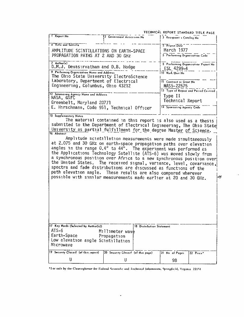
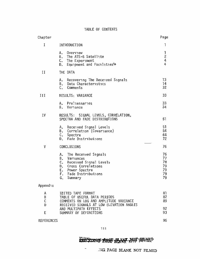
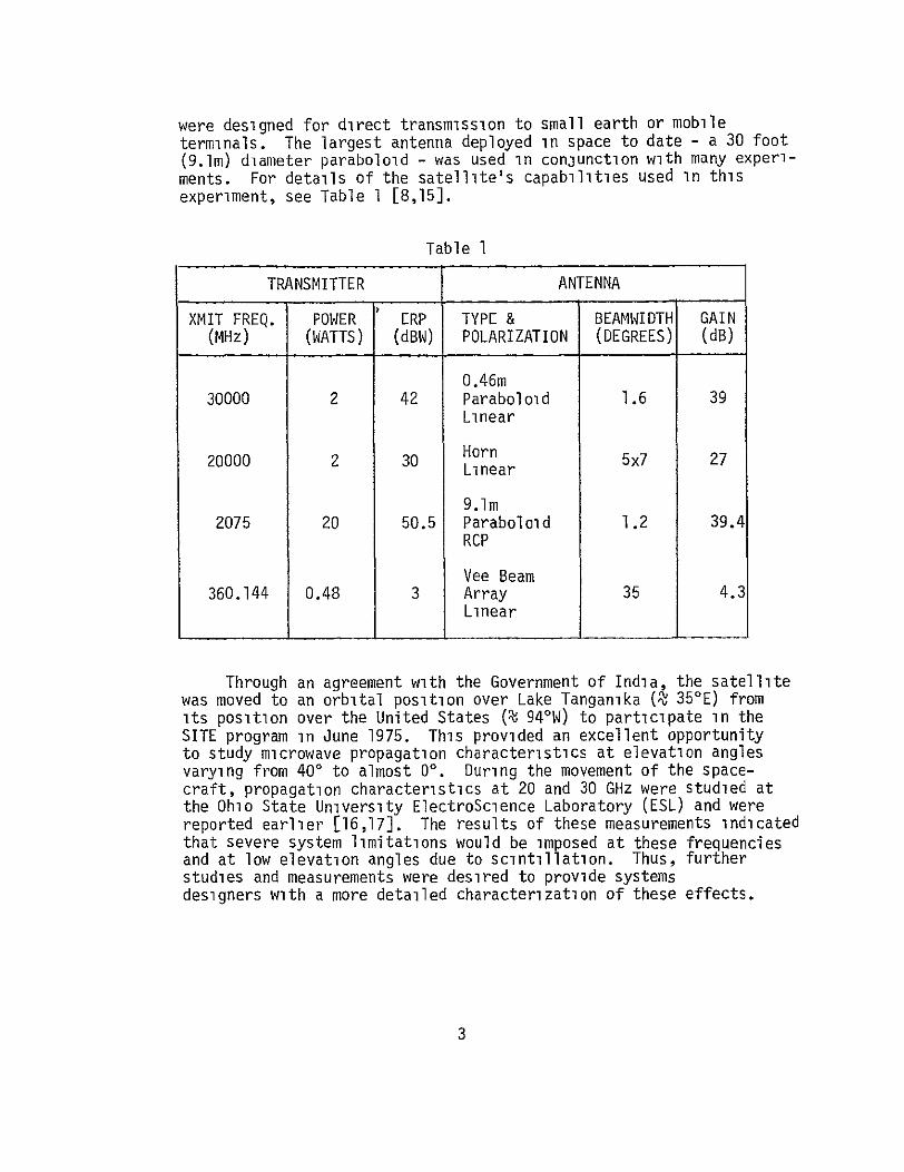
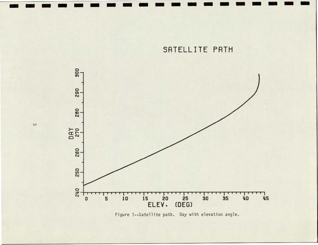
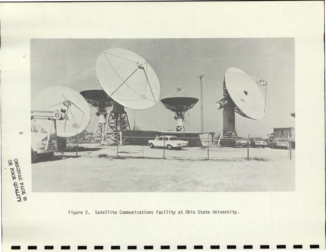
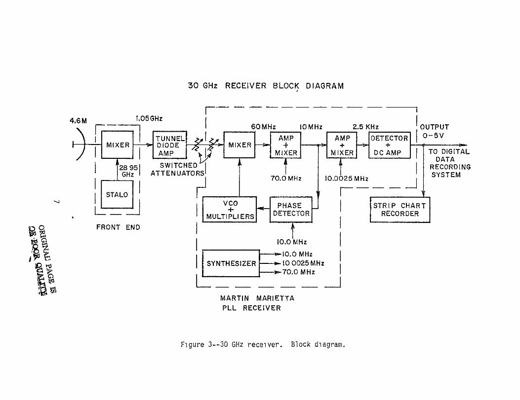
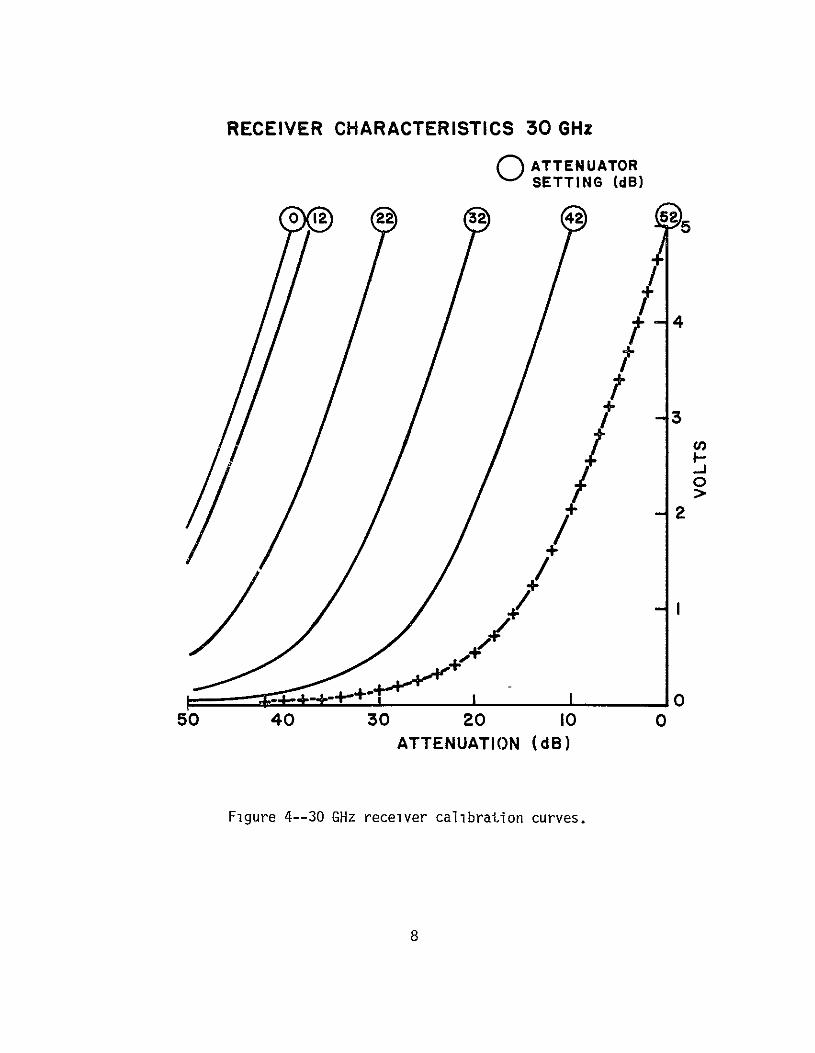
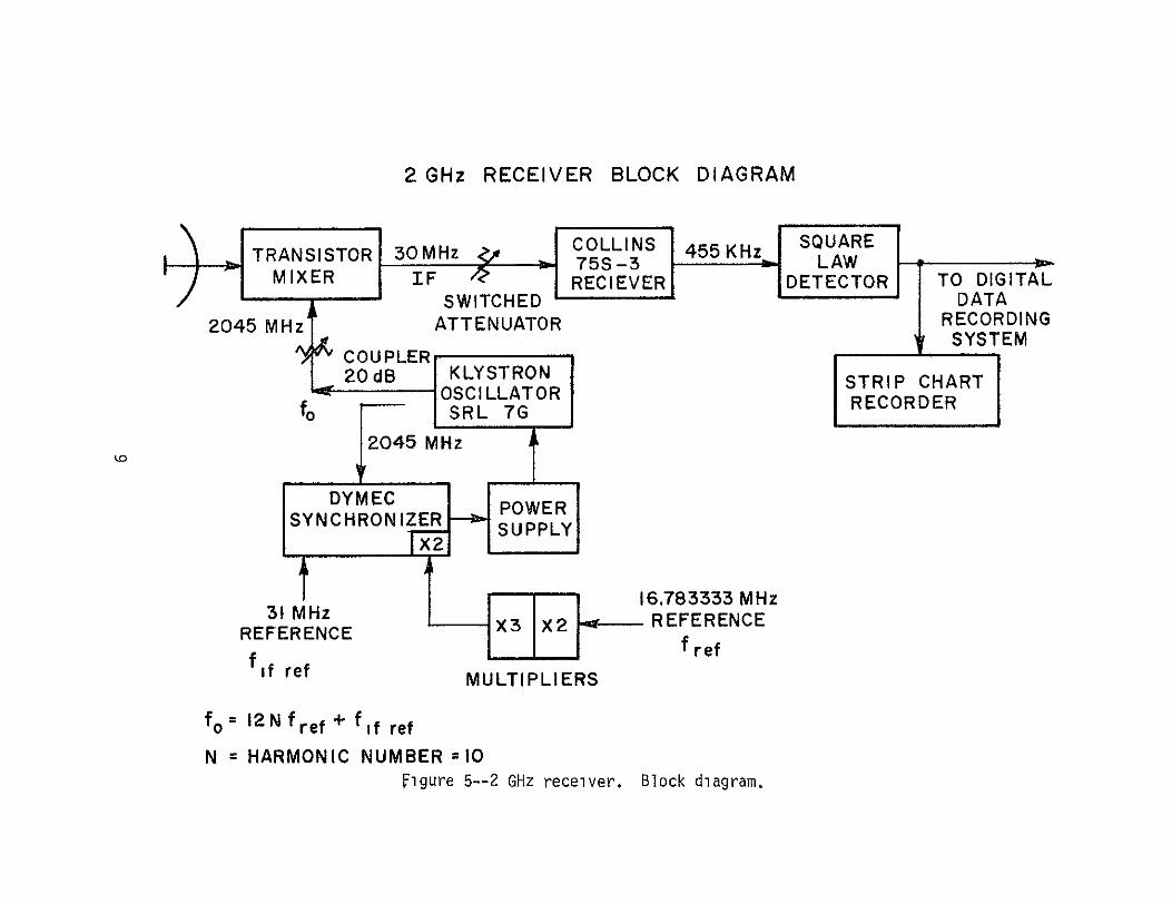
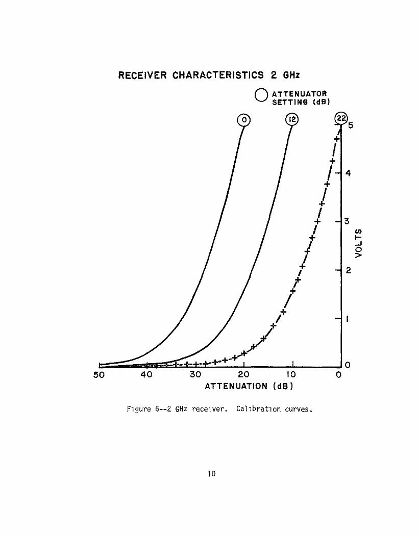
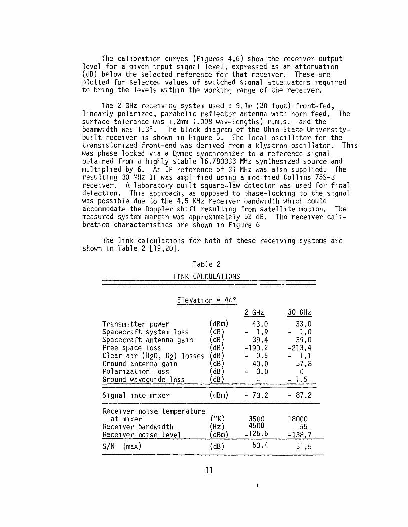
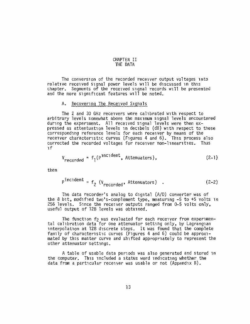
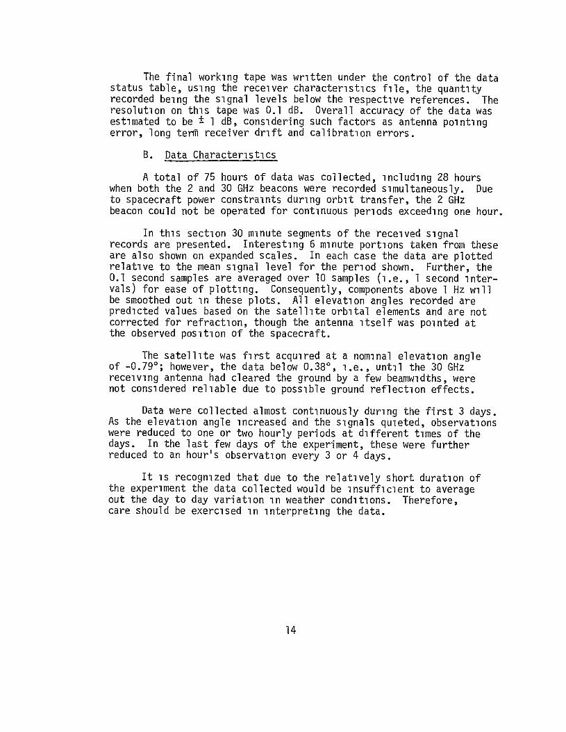
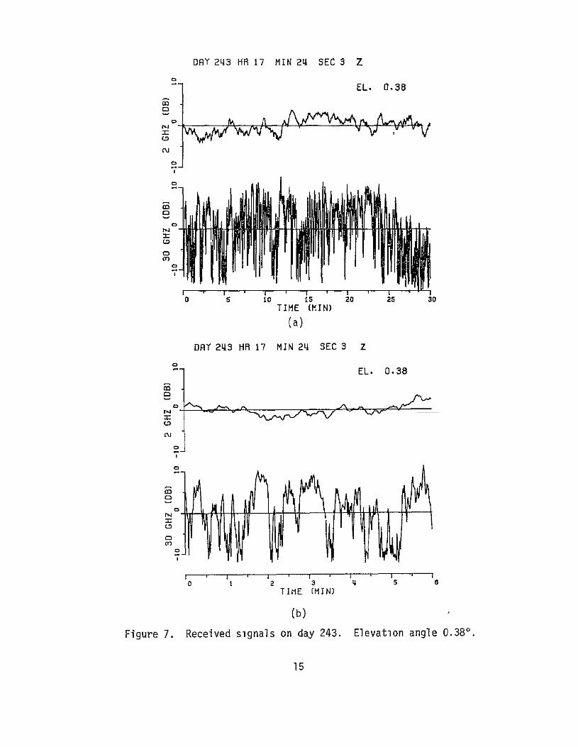
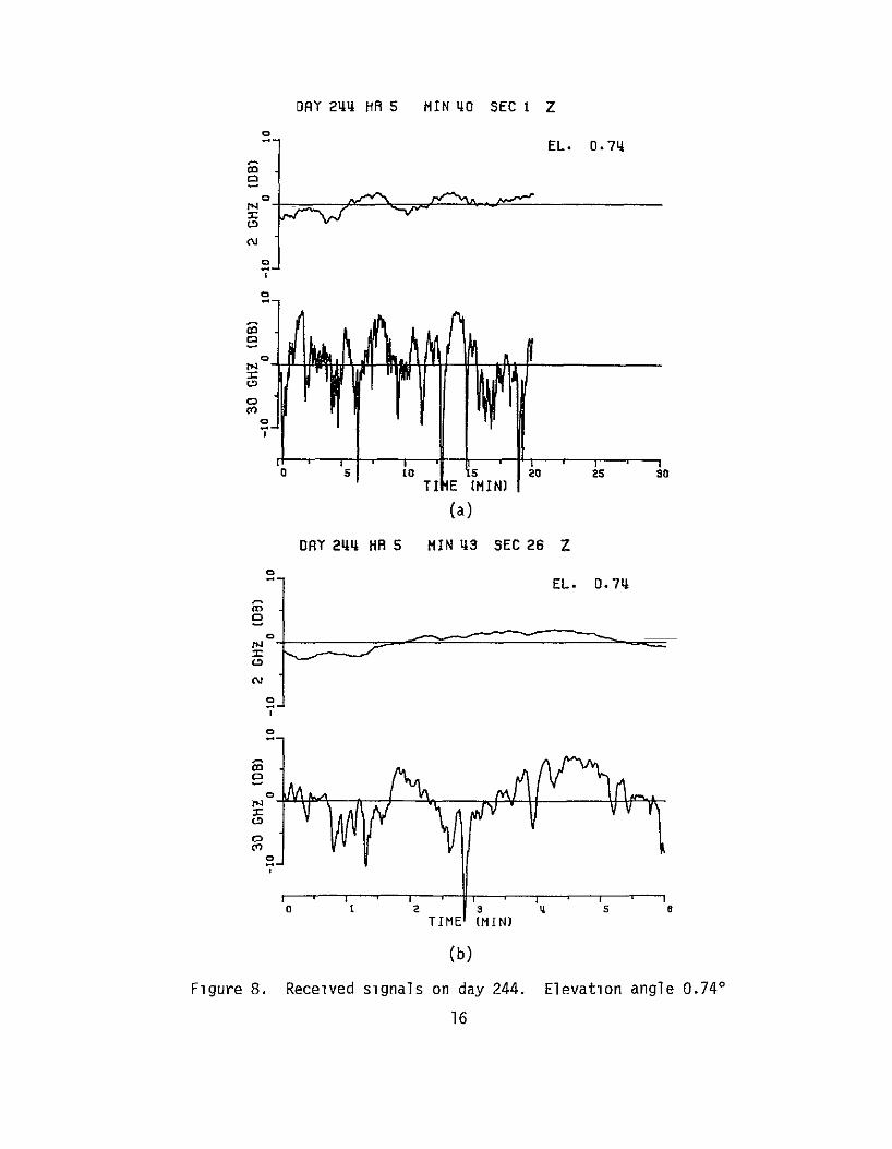
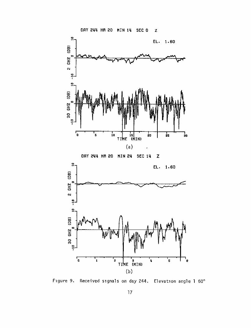
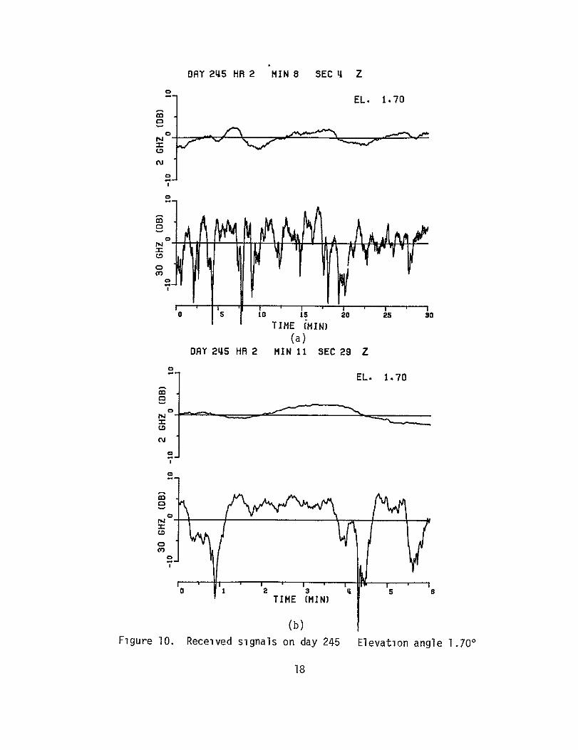
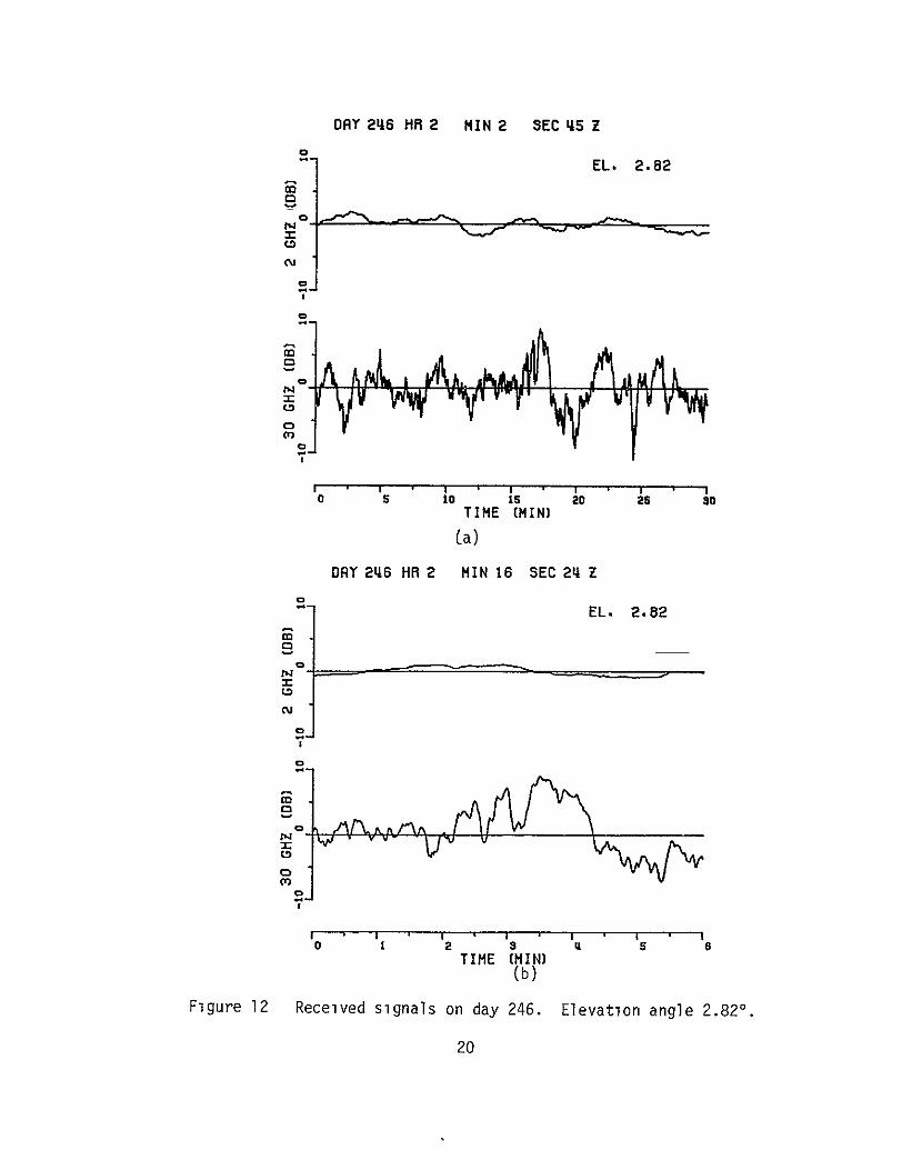
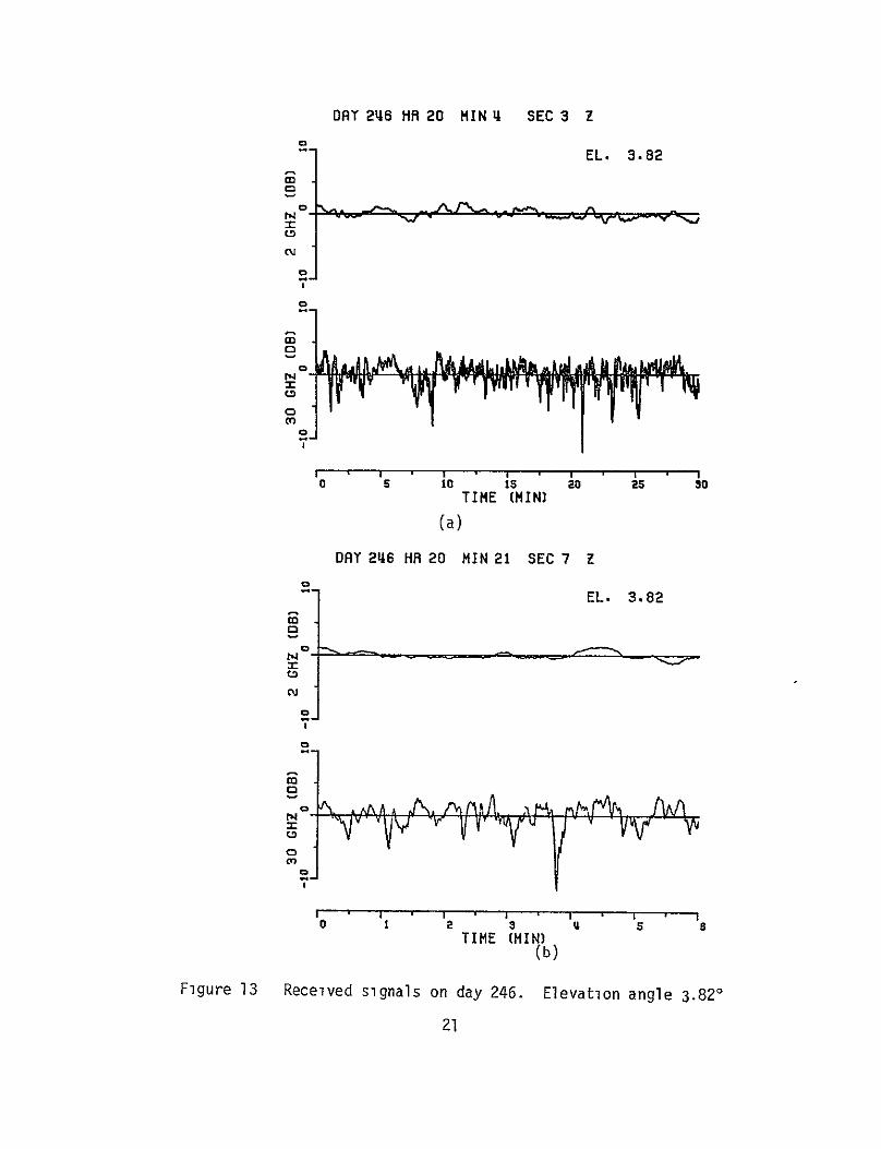
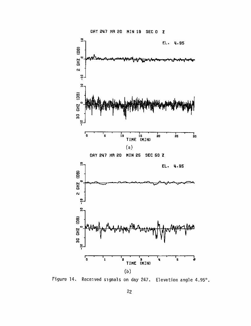
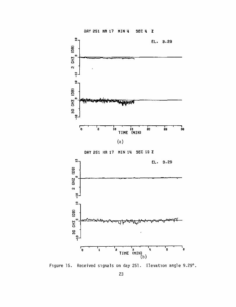
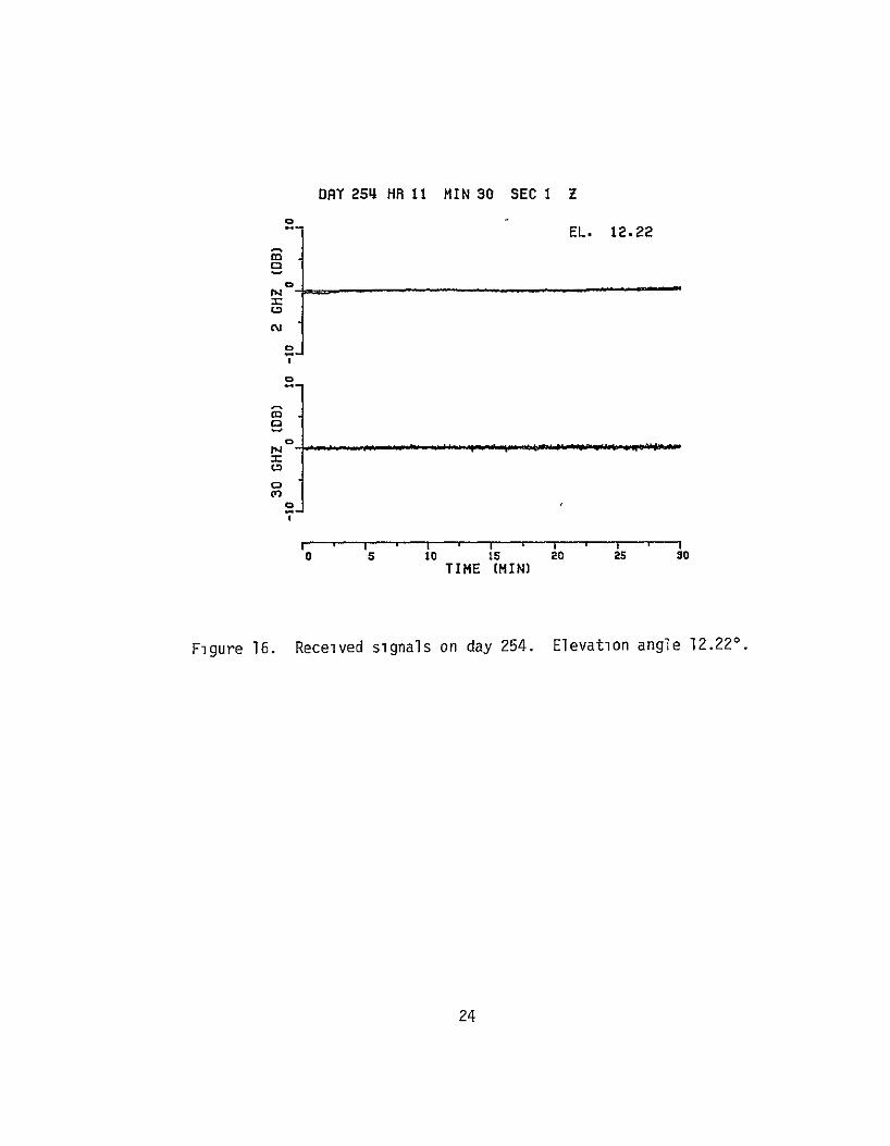
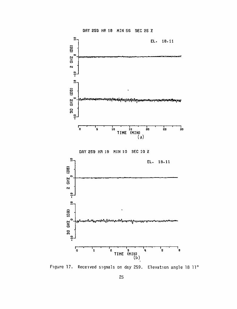
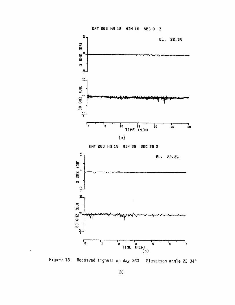
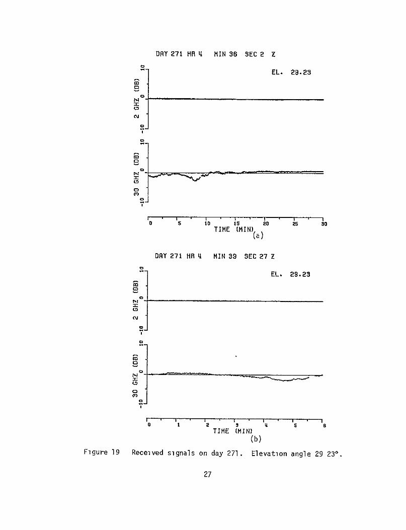
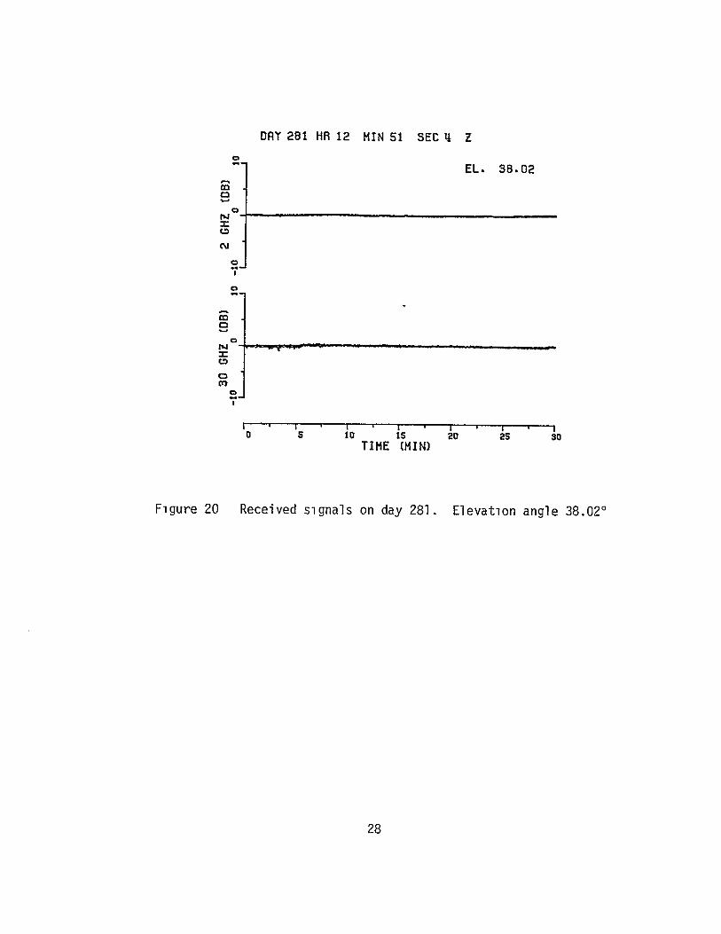
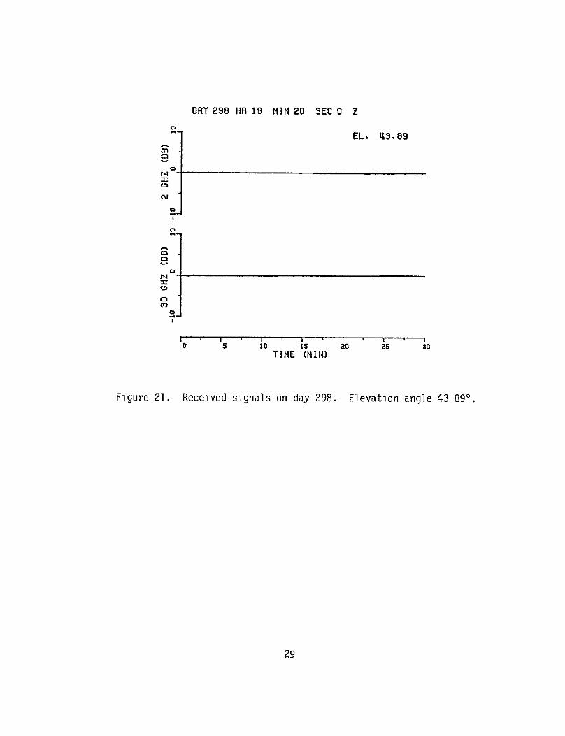
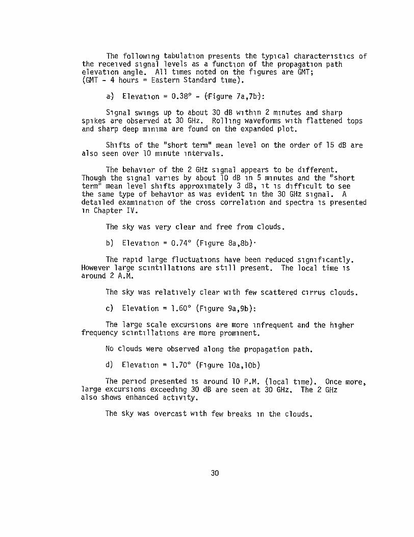
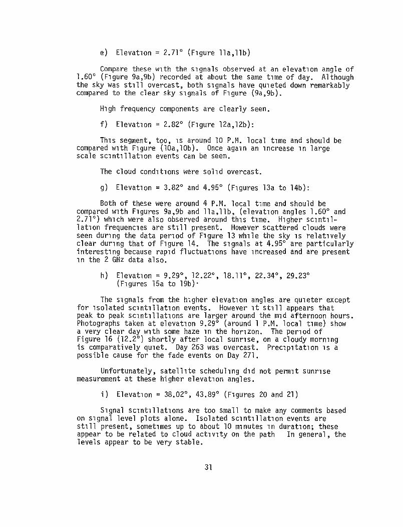
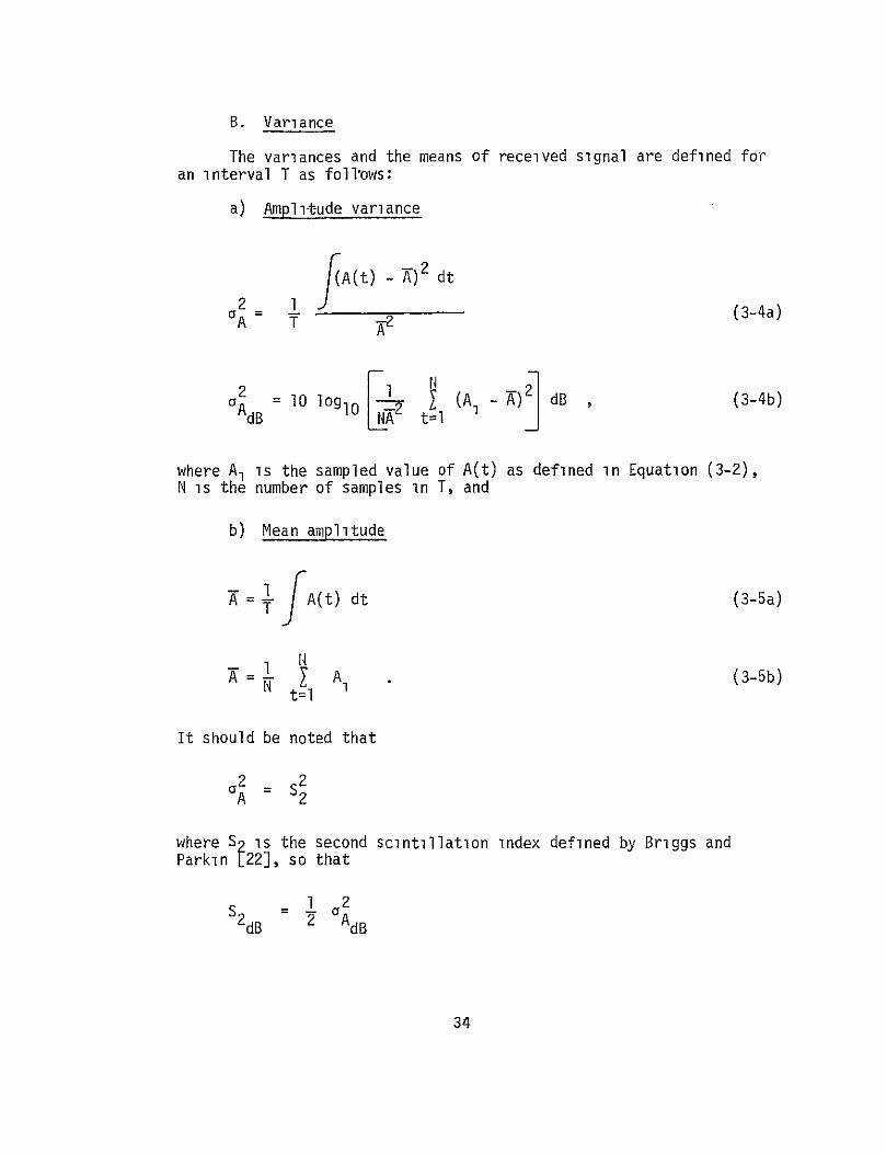
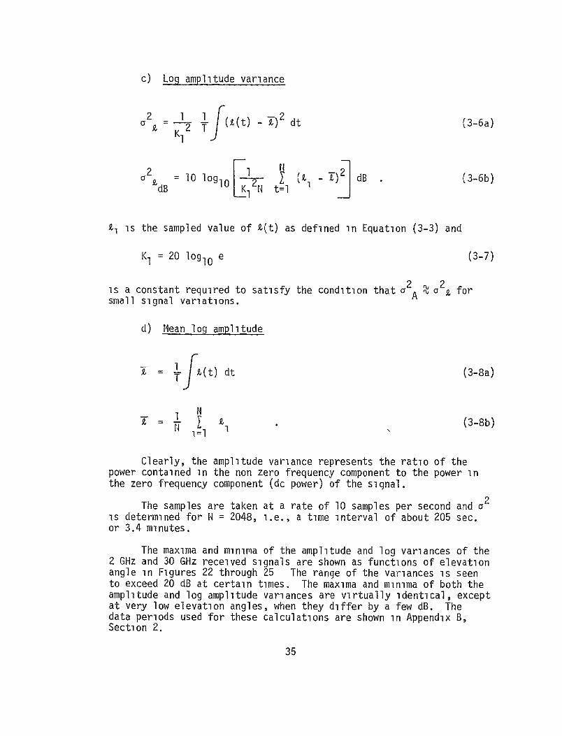
2
c) Log amplitude variance
2 1 1 (t) 2 (3-6a) 2 T ) -()t) (3-6a)
K1
= I0 lOglo 1 T2dB (3-6b)
dB 1 r t=l
Pi is the sampled value of L(t) as defined in Equation (3-3) and
K1 = 20 lOglo e (3-7)
is a constant required to satisfy the condition that aA a2 for small signal variations
d) Mean log amplitude
1 t) dtT (3-8a)
=1 N
T = j_ (3-8b)
Clearly the amplitude variance represents the ratio of the power contained in the non zero frequency component to the power In the zero frequency component (dc power) of the signal
2 The samples are taken at a rate of 10 samples per second and a
is determined for N = 2048 ie a time interval of about 205 sec or 34 minutes
The maxima and minima of the amplitude and log variances of the 2 GHz and 30 GHz received signals are shown as functions of elevation angle in Figures 22 through 25 The range of the variances is seen to exceed 20 dB at certain times The maxima and minima of both the amplitude and log amplitude variances are virtually identical except at very low elevation angles when they differ by a few dB The data periods used for these calculations are shown inAppendix B Section 2
35
o VARIANCE
+ 2 GHZ
0
C2 _
gtlt
00
CA)CD
CO
Fi gure
0 o
22
10 15 20 25 so 5 40 45
ELEV (DEG)
Amplitude variance Maxmin 2 GHz with elevation angle
LOG VRRIRNCE + 2 GHZ
0
C
0 -
Xl
O
I- I
0 5 10 15 20 25 30 35 10 45 ELEV (DEG)
Figure 23 Log amplitude variance Maxmin 2 GHz with elevation angle
VARIANCE
X 30 GHZ
M
000
so I T
X0 in
203
0 5 10 1 0 25 3 5 amp 1 ELEV WDEG)
Figure 24 Amplitude variance Maxmin 30 GHz with elevation angle
C7
LOG VRRIRNCE
X 30 GHZ
C3
Cshy
0T
C
0
Figure 25
5 10 15 20 25 ELEV (DEG)
Log amplitude variance Maxmin
30 35 40 45
30 GHz with elevation angle
Next it was assumed that the variances followed the law
02 = ALB (3-9)
where L is the path length of the received signal through the atmosphere and A and B are constants If the elevation angle is denoted by 8 then for a plane earth with an atmosphere of finite thickness
L - CSC(o) (3-10) 2
A minimum-mean-square-error curve fit to a2 = A [CSC(e)] B was performed for all the variance values obtained in this experiment The results were
Amplitude variances
a2A2 10-49 [CSC(e)]1 62 plusmn 2 (3-11)
2 [CSC(e)] 214 plusmn 3 (3-12)
A30
Log amplitude variances
02 = 10-49 [CSC(O)J 162 plusmn 2 (3-13)
2 = CSCOA220 t 3 (3-14) 30
Thesubscript on the variance denotes the frequency
Kolmogorov turbulence would give a relationship of the form [23]
aL11 6 aL1 8 33 G2 = = (3-15)
These results appear to be in fair agreement with the 2 GHz results somewhat below and the 30 GHz results above the theoretical value
40
The average amplitude and log amplitude variances at each elevation angle together with the fitted cosecant law curves are shown in Figures 26 and 27 As is to be expected this law breaks down at very small elevation angles due to the plane earth assumption
In order to improve the fit a spherical earth with a uniform atmosphere of height h was next assumed (Figure 28) The effective radius R of the earth was taken to be 43 the actual radius or 8479 km in order to compensate for standard refraction The radio waves may then be assumed to propagate in straight lines The path lengthL within this equivalent atmosphere is then-
L = h2+2hR+R 2sin 2e - Rsine (3-16)
Equation (3-9) was again fitted to all the variance values in the minimum mean-square-error sense but with the path length L givenby Equation (3-16) above The equivalent height parameter h was also a variable and was adjusted to minimize the error The compushytation was continued until successive values of h converged to within 001 km for best fit
The results are-
Amplitude variance
a2 = 10-65 L1 87 plusmn 2 (3-17)
h = 62plusmn1 km (3-18)
2 10-64 L24 8 plusmn (3-19)A30
h = 60plusmn1 km (3-20)
Log variance
2 = 10-64 L187 plusmn 2 (3-21)pound2
h = 61plusmn1 km (3-22)
2 = 10-61 L249 plusmn (3-23) a 30
h=45plusmn1 km (3-24)
41
o_ VRRIRNCE + 2 GHZ X 30 GHZ
I X
Cj- x+
X n 1 +
+ +
+ X + 0
gt30 +
INI
0 5 10 is 20 25 so 35 40 45 ELEV (DEG)
Figure 26 Mean amplitude variance with elevation angle Cosecant law
2 LOG VRRIRNCE + 2 GHZ
0 X 30 GHZ
2
N 4shy+
4-
4- x W r +-t
X X xizx X - x X x
+ + x --- +++ ++-+shy
o +
0 5 10 15 20 25 30 35 q0 15 ELEV (DEG)
Figure 27 Mean log amplitude variance with elevation angle Cosecant law
Figure 28 Ray geometry for a - spherical earth
The average amplitude and log amplitude variances at each elevation angle together with the fitted spherical earth law curves are shown in Figures 29 and 30 The amplitude and log amplitude variance curves are almost identical except at the very lowest elevation angles
The reduction in mean square error using the spherical earth model ranged from 5 to 15
The value of the equivalent height parameter h is strongly dependent on low elevation angle data
Figure 31 also shows the average amplitude variances togetherwith the 30 GHz variance data derived from the earlier set of measureshyments made in 1975 during the departure of the ATS-6 [17]
The 1975 results agree well with the recent values The cosecant law relationship found for the earlier data was [171
a2AA30 (1975) = 10-36 [CSC(O)]J1 90 (3-25)
which agrees fairly well with that shown in Equation (3-12)
44
_ VARIANCE + 2 GHZ X 30 GH
0
I
x
lshy
(UDEG) ELEV
C +
~ 25 30 I 45 1 20 35 40
ELEV (DEG)
Figure 29 Mean amplitude variance with elevation angle Spherical earth model
LOG VRRIRNCE + 2 GHZ X 30 GHZ
I x X
I- +
CD V u 30 Ma o i v
0 5 10 s1 20 25 s0 35 10 415
ELEV (DEG)
Figure 30 Mean log amplitude variance with elevation angle Spherical earth model
o VARIRNCE
3
x 30GHz 1976
7-0
+ 30 GHz
2 GHz 1975 1976
+XX
-
-40
4i
S+
Cshy+
++
_
Cr + Xx
+-
x
4+
x0 0
XXX + +
+-++ +
x
4+
x
+
x
+
x
+ +
0
0
In
a
0 5 10 15 20 ELEV
25 (DEG]
30 35 q0 45
Figure 31 Mean amplitude variance with elevation angle 1975 and 1976 results
Also at 20 GHz
872 (1975) = I0-40 [CSC(e)]1 (3-26)A20
The fairly large error bounds have been introduced in the presentresults not to indicate uncertainty in the data itself but to take into account the limited duration of the data and the correcting effect that observations over extended periods of time under different weather conditions would have on the results
The ratio of he amlitude variances of the 30 and 2 GHz received signals (aA30a A2 ) is shown in Figure 32 While it is
difficult to draw any reliable conclusionsfrom this it is observed that the average value over all the elevation angles is 92 dB Similarly a value of 44 dB was obtained for 2A na2A20 (ie for
30 and 20 GHz) during the departure of ATS-6 [17 However in this case there appears to be a tendency for this ratio to decrease as the elevation angle increases
An example of the behavior of amplitude variance with time is illustrated in Figure 33 The corresponding received signals are shown in Figures 14a and 14b This figure illustrates more clearly the manner in which the variances are affected by short periods of enhanced scintillations observed in Figure 14 and also shows how closely the 2 and 30 GHz variances track each other at this elevation angle It suggests that the cross-correlation of the signals be examined This is done in the next chapter
48
VAR 30VRR 2
-4xx
X
x -4 XX
x C2
x XX x x
Sx X x
CO XXx
CUC x x
x
ELEV (DEG)
Figure 32 Ratio of variances a2 Cy with elevation angle A30 A2
VARIANCE WITH TIME
+ 2 GHz X 30 GHz
-10 V EL 490
TIME 247 20 22Z
- X - X
-15
W-20 z
-30 I I I I I 0 200 400 600 800 1000
TIME (SEC)
Figure 33 Amplitude variance with time day 247
50
CHAPTER IV RESULTS- SIGNAL LEVELS CORRELATION
SPECTRA AND FADE DISTRIBUTIONS
In this chapter the average received signal levels are shown The correlation between the signals is discussed in detail The correlation results are compared with those predicted by the Lee and Harp model and good agreement is found Some representative samples of correlation as a function of time lag are shown Lags are in the range of 0 - 10 seconds with most of the values being around 0 - 5 seconds
The power spectra are considered next A characteristic decay is found in the 01 to 1 Hz range This decay follows the f-83 law
Fade distributions are also shown These are in general Gaussian except for anomalous cases which appear to point to some other mechanism Standard deviations calculated from the Gaussian models agree reasonably well with those calculated directly in Chapter III
A Received Signal Levels
The mean relative power in the signal is defined as
2ea (4-la)Mean Power = f t t(-a
A 2= 10 loglo dBj (4-1b)
with T = 205 seconds as before The mean power averaged over each elevation angle is shown in Figure 34 As expected the mean log amplitude (Figure 35) and mean power are virtually identical The sharp reduction in signal level at an elevation of 93 is due to the fact that the spacecraft antennas were directed toward Texas for another experiment on that day
A substantial reduction in the received power level below that predicted by simple atmospheric path loss calculations [24] at the lower elevation angles is also noted this behavior has been observed earlier by McCormick and Maynard [25]
51
a POWER + 2 GHZ X 30 GHZ
+ ++++++++ ++ + +
XX Xxx xxXX x X X x
0 TEXAS (n- POINTING
T
to- x
IDshy
0 5 10 15 20 25 s0 35 40 45 ELEV (DEG)
Figure 34 Mean relative power in the signal with elevation angle
2 LOG RMPLITUDE + 2 X 30
GHZ GHZ
+
X
+ x X x
++
X
+ xx
++ X Xx x
+ K
CsJ
-I
0 TEXAS POINTING
0
OX C3
o shy
5 10 15 20 ELEV
25 (DEG)
30 35 43 q5
Figure 35 Mean relative log amplitude of the signal with elevation angle
The more pronounced variations in the 2 GHz mean power at the
higher elevation angles is believed to be due to equipment problems
B Correlation (Covariance)
The terms Correlation and Covariance are used interchangeably in this report and both denote the correlation functions defined for lag T by
( 2(t+T)-T21 dt If(t-)
P2(T) = T
12 FT f(pt)T)2d~t l f 2 t)w )2d~t 2
(4-3)
where denotes either the log amplitude Z or the amplitude A and T is 205 seconds Therefore
N (A2 - T2)(A30 -A30 )
1 i=l 1+J (4-4) A230 2A30 A2 aA30
N1(Z2A1 - 2) (1+J 3 0 - T30 )
(pound2 (4-5) 230 KI2N dega2 P30
T
These correlation functions are equal for small scintillations
The log amplitude and amplitude peak correlation coefficients are averaged at each elevation angle and plotted in Figure 36 Although some divergence is found at the lowest elevation angles they are found to agree well at higher elevation angles
It should be noted that the effective separation between the antennas varied from 102 meters at 04 to 73 m at 4380 This separation tends to reduce the observed correlation values
54
CROSS CORRELATION
CD
o
8shy
0
x
+
X
LOG AMPLITUDE
AMPLITUDE
(119
00
C)
0 5 10 15 20
ELEV
25
(DEG)
30 35 40 q5
Figure 36 Cross correlation with elevation angle
Although there appears to be no theoretical justification the curves are again suggestive of a cosecant law A minimum-mean-square error curve fit was made to test this and the results were
Amplitude Correlation
(4-6)PA = 059 [CSC(e)]1 62 plusmn3
Log Amplitude Correlation
pZ = 059 [CSC(e)] 166 plusmn 2 (4-7)
230
These are also plotted in Figure 42
It is interesting to note that these exponents also lie in the range of the values calculated earlier for the CSC(e) exponent in the case of variance
Next the Amplitude Correlation Coefficient obtained was compared with the theoretical value predicted by Lee and Harp [26] for this frequency ratio of 1446 The covariance between the 2075 and 30 GHz signals is shown in Figure 37 together with the theoretical curve of Lee and Harp Although the spread of the covariance is large the average over the entire data base agrees well with the theoretical prediction Also included are the results for the 20 and 30 GHz data obtained earlier [17]
As the cosecant law suggested by Figure 36 appeared to be a good approximation the covariance was also plotted against CSC(e) Howshyever Figures 36 and 37 show a wide range of values for the correlation coefficient but do not show its behavior over ranges of elevation angles of interest Therefore the correlation coefshyficient was next averaged over selected elevation angles and shown in Figure 38 together with the Lee and Harp value The agreement is now seen to be very good for elevation angles up to about 50 ie in the region where the signals are being affected the most Somewhat surprisingly the correlation is seen to fall off to nearly zero at the higher elevation angles ie the region of weaker turbulence effects
It should be noted that the path length was constantly changing during the experiment while the Lee and Harp curve was calculated for a fixed path length This and the change in the effective separation between the antennas should be considered in evaluating the agreement with the theoretical value
56
I0
08 W 0
zgt 06
---1975
0
DATA
E AVE AVE
FOR EACH OVER ALL
DATA DATA
PERIOD PERIODS
00
a4
t04 -J a
r LEE as H-ARP
1 2
Figure 37
4 6 8 10 20 FREQUENCY RATIO
Cross correlation with frequency ratio
40 60 80 100
04 CORRELATION WITH
CSC ( ELEVATION) X
x 03shy
x
LEE a HARP K
0C
S0
euron XK X x coo KAMP PEAK CORR
x LOG AMP PEAK CORR SI--i LOG AMP PEAK CORR
AVERAGED OVER SELECTED ELEVATION ANGLES
-01-) ELEVATION (DEGREES
50 10 5 I 05 01-02 I h111 I lll I Ililig 10 100
CSC (ELEVATION)
Figure 38 Cross correlation averaged over selected elevation angles with cosecant (elevation)
1000
Some examples of cross-correlation and auto-correlation funcshytions of the received signals are presented in Figures 39 through 46 It was observed that over a period of a record (ie 205 seconds) significant shifts of the mean level occurred This would tend to make the process non-stationary Consequently a correction was applied to the record being analyzed by assuminq that the mean-shift was linear with time over the interval of the record This correction narrows the peak of the correlation functions ie reduces the interval of high correlation values which would otherwisebe obtained
The lags associated with the maximum values of the cross corshyrelation were in the range of 0 - 10 seconds with most of the values in the region of 0 - 5 seconds It also appeared that significant correlation was lost for lags exceeding about 15 seconds
The effects of various wind fields on the correlation function have been studied in [26] The lag of the peak correlation is shown to depend on the wind velocity across the propagation path and the shape of the curve on the wind distribution The double hump in Figure 41 for example may be attributed to non-uniform wind fields
59
AUTO-CORRELATION
EL 038
TIME 243 1727Z o 30 GHZ
AMPLITUDE
C
to
10 -80 -60 -q0 -20 0 20 40 so so800 LRG (SEC)
Figure 39 30 GHz amplitude autocorrelation function at
eleVation angle 038
AUTO-CORRELRTION
EL 038
TIME 243 17277
_ 30 GHZ
LOG AMPLITUDE
Ushy
cc
-1o0 -80 -60 -40 -20 LAG
o 20 (SEC)
40 so 8o 100
Figure 40 30 GHz log amplitude autocorrelation function at 0 38
60
CROSS-CORRELRTION
EL 038
TIME 213 1727 o AMPLITUDE
IL
-
C 4
10o -80 -s0 -40 -20 0 20 40 so so 20D LAG (SE--)
Figure 41 Amplitude cross correlation function at 0380
LU0
L) CROSS-CORRELAITION
EL 038
TIME 243 1727Z
o LOG AMPLITUDE
8shy
-100 -80 -80 -10 -20 0 20 o so 80 100 LRG (SEC)
Figure 42 Log ampltude cross correlation function at 0 380
61
CROSS-CORRELRTION
EL 495
TIME 247 2029Z o AMPLITUDE
UJ
C
tzOil -0 6 -40o -20 rl 20 40 60 80 100LAG (SEC)
Figure 43 Amplitude cross correlation function at 4950
cJ cc
- CROSS-CORRELATION
EL 929
TIME 251 171t4Z
o_ - AMPLITUDE
o -oo -so -60 -w -20 0 20 40 s0 80 100
LAG (bEC)
Figure 44 Amplitude cross correlation function at 9 290
62
CROSS-CORRELATION
EL- 22-31i TIME 263 1839Z
o AMPLITUDE
U-
C
C-
-100 -80 -Be -140 -20 a 20 40 6C) 80 10o LRG (SEC)
Figure 45 Amplitude cross correlation function at 22340
RUTO-CORRELATI ON
EL 113-89
TIME 298 1820-7
o2 GHZ
AMPLITUDE
8shy0
0 -80 -80 -0 -20 0 20 140 0 80 100 LRG (SEC)
Figure 46 2 GHz amplitude auto correlation function at 43890
63
C Spectra
Sample spectra of the received signal are shown in Figures 47 through 53 Corresponding records of received signal will be found in Figures 7 through 28 These spectra all show a characteristic decay with frequency in the range from approximately 01 Hz to 10 Hz The spectra tend to be relatively flat outside that range
The slope of the spectra in the decaying region was measured manually for several samples The results of 12 samples each at 2 GHz and 30 GHz are shown in Table 3
Table 3
SLOPE OF SIGNAL SPECTRA
2 GHz 30 GHz dBdecade dBdecade
MAXIMUM 306 312
MINIMUM 235 200
MEAN 255 268
These results agree closely with a power roll-off relationship of the form f-8 3 or 267 dBdecade This result also agrees with the assumption that a tropospheric turbulence mechanism is producingthe observed scintillations [27]
64
O POWER SPECTRUM
2 GHl RECEIVER EL 038
ai0 TIME 243 1727Z SCU
C
-j LUEDm
0
0
FREQ IN HZ
(a)
OPOWER SPECTRUM
30 GHZ RECEIVER
EL 038 0 TIME 243 1727Z
-C
U
jco
FREQ IN HZ
(b)
Figure 47 Power spectra at 0 380
65
o POWER SPECTRUM
2 GHZ RECEIVER
EL 160 TIME 244 2024Z
=7- N EU
degx
FREQ IN HZ
(a) Cr
U
LI S-Jo o POWER SPECTRUM
~30 GHZ RECEIVER
ccEL 180 wo TIME 244 2024Z
FREQ IN HZ
(b) Figure 48 Power spectra at 1600
66
_ POWER SPECTRUM
2 GHZ RECEIVER
cc L
EL TIME
282 216 2 16Z
-
cc
(a)
U
~POWER SPECTRUM
C IL 30 GHE8RECEIVER
co
UOTIME 246 2 16Z
C
-J
FRE IN HZ
(b)
Figure 49 Power spectra at 2820
67
o POWER SPECTRUM
2 GHZ RECEIVER EL 495
U TIME 247 20292
a
J
LU 0
FREQ IN HZ
(a)
oPOWER SPECTRUM
30 GHZ RECEIVER EL 495
L TIME 247 2029Z
cc - U
a S-
FREQ IN HZ
(b)
Figure 50 Power spectra at 495
68
C POWER SPECTRUM
2 0HZ RECEIVER EL 1811
o TIME 259 1913Z
a 0
m-J
FREQ IN HZ
(a)
o_ POWER SPECTRUM
30 GHZ RECEIVER EL 1811
Uj TIME 259 1913Z
oIm
FREQ IN HZ
(b)
Figure 51 Power spectra at 18 110
69
o POWER SPECTRUM
2 GHZ RECEIVER EL 2234 TIME 263 1842Z
-C
aCr
L)
CD
C
FRED IN HI (a) 0H
oPOWER SPECTRUM
30 GHZ RECEIVER EL 2234 TIME 263 1842Z
-c
m I
FREG IN HZ (b)
Figure 52 Power spectra at 2234
70
b
o POWER SPECTRUM
2 GHZ RECEIVER
EL 4389 TIME 298 1850Z
Cr
C
-J
FREQ IN HZ
Figure 53 Power spectrum at 43890
71
D Fade Distributions
Fade distributions were also studied at several elevation angles averaging about 30000 samples ie 50 minutes each Figures 54 and 55 show the percentage of time a given fade depth was exceeded plotted on a log-normal scale
The curves appear to fit fairly well within each other with increasing elevation However exceptions are clearly seen at 038 and 1600 for both 2 and 30 GHz and at 495 for the 2 GHz signal The reason for the behavior at 495 is not clear at present It should be noted that the 30 GHz fade distribution at this elevation angle does not behave in the same way
The distributions at 2820 are taken to be a representative sample for the higher elevation angle cases and show good fit to straight line approximations indicating that they are Gaussian Even the anomalous distributions show a Gaussian nature over a large portion of their ranges
The fade distributions could in fact be a combination of more than one type of statistic Deviations from the Gaussian curve are prominent for large scintillations Furthermore since the sampling rate is high (10sec) it is possible that the effects of rapid short term scintillations which are believed to be Rayleigh distributed are also being displayed in these distribution curves [28]
Assuming that the dominant long-term statistics at-the higher elevation angles are Gaussian a check was performed at 2820 as follows Let the un-normalized variance be s2 For a log-normal distribution the interval between the 50 and 999 percentile values of the cumulative distribution function - ie 50 and 01 pershycentile values of the fade distribution function - is 31 s[29] For 30 GHz from Figure 55
31 s30 = 86
=27s30
Now from the definition of a2 (Equation (3-6)) we can write that
0 ogloG2 =
dB K1
2zdB
= K110os
72
9999 FADE DISTRIBUTIONS
2 GHz 999 998 -
99 gtt
AA A
ELEVATION (DEG)
98 bull A 0
X 038 160
95 9-0D A o628228 04 A 495
90 x 0 1811 + 1+ 4381
x c0 o X
w 70 x w + E3
x 60shy
lt 50 + 40- 13
350- 0 0
C20 + x
1-0- A3 X x~
ox x 5-+ C X
+ A x X XX
2 I-
+ A
05 a
02- 0
0I 005
001 0 1 5 4 5 6 7 a 9
FADE (d8)
Figure 54 Fade distributions at 2 GHz
73
9999
999
998 -
FADE DISTRIBUTIONS
30 GHz
w w o x
99
98
95
80
A
X
x
ELEVATION (DEG)
038 x 160 0 282 A 495
1811 + 4381
600
650 a
S40 -x
w30-
-20 20
A
A x 0
10-0+D
0+ 0 5-
2--x 5
A30
Abull 0
X
0
S
X X
X OX x
2- A X
02- I A- 0 0 x
021
0010 5 10 15 20 25 30 35 40 45
FADE (d8)
Figure 55 Fade distributions at 30 GHz
74
From Figure 27 average log amplitude variance at 282
2 a ZdB 30 = - 115 dB
-115
s30 = (20 loglo e) 1 010
s30 = 234
This compares favorably with s as calculated from Figure 55
Similarly for 2 GHz at 282 from Figure 54
31 s2 = 23
= 074s2
from Figure 27 and following the same procedure as above
s2 = 045
The discrepancies could be partly due to the fact that the values shown in Figure 27 are calculated for 205 second intervals only and then averaged over each elevation angle These are therefore shortshyterm statistics and would tend to be Rayleigh distributed whereas the distributions in Figures 54 and 55 were calculated over the whole elevation angle directly these tend to be Gaussian Further the deviations from the log-normal curve for strong scintillations would also affect the result
75
CHAPTER V CONCLUSIONS
The results of the experiment are summarized in this chapter
A The Received Signals
The received siqnals show several types of fluctuations
a) Very low elevation angles (less than 40)
(i) Slow rises and fades of tens of dB over periods of tens of minutes
(ii) Faster fluctuations or scintillations with durations of a few minutes or less occurring continuously
(il) Continuous rapid scintillations of a dB or less
(iv) Slow roller-type fading is also seen However the high signal correlation found rules out ground reflection effects (Appendix D)
b) Low elevation angles (40 to 100)
(1) Very slow changes in mean level of a few dB over 30 minutes or more
(ii) Faster scintillations of several dB with periods of a few tens of seconds
(il) Continuous rapid scintillations
c) Medium elevation angles (10 - 44)
(1) Virtually no change in mean level except during precipitation events
(ii) Enhanced scintillations of a few dB for a few minutes are now visible
(iii) Continuous rapid scintillations
Scintillations were observed at all times in clear air and also in the presence of non-precipitating clouds At the highest elevation angles there appears to be a tendency for the scintillations to be enhanced in the presence of non-precipitating cumulus clouds
76
In the following discussion the symbols A and k are used to denote amplitude and log amplitude quantities respectively The symbol V is used to denote either one in general
B Variances
Amplitude and log variances are defined in Equations (3-4) and(3-6)
The range of the variances at any elevation angle exceeded 20 dB at times However the average variances followed a cosecant power law with elevation angle fairly well
Table 4
2 A [CSC(EL)] B
2 GHz 30 GHz
A B A B
10-4 9 12 162 10-4 3 214A 2 plusmn3
-43 a 2 10-49 162 10 220plusmn2 plusmn3
The fairly large error bounds have been introduced to account for the limited data Observations over extended periods under widely varying weather conditions would give a closer estimate The exponents B compare well in their range of error with the theoretical value B = 1833 for Kolmogorov type turbulence
As a refinement a spherical earth model was assumed with a uniform homogeneous atmosphere of effective height h km When this was fitted to the data the results were as follows
77
Table 5
a2 -A LB
L =Ih2 + 2hR + R2 Sin2e - RSine
R = 8479 km 0 = elevation anole
2 GHz 30 GHz
A B hkm A B hkm
10- 6 5 10- 6 4A 187 62 248 61plusmn2 plusmn1 plusmn3 plusmnI
2 10-6 4 187 61 1061 249 45
plusmn2 plusmnIt3
A reduction inmean square error of between 5 to 15 is obtained However in general the much simpler cosecant law
a A [CSC(amp)]B
appears to be quite adequate for elevation angles above 40
The 30 GHz data obtained during the departure of ATS-6 in 1975
agree well with the present data
The ratio of variances a2 1 2 has a mean value of 92 dB
A value of 44 dB was obtained for a2A30l 2A inthe 1975 measureshyments 3
C Received Signal Levels
The relative received signal levels show a strong dependence on elevation angle for elevations less than 5 They are relatively independent of elevation thereafter The drop in signal levels at low elevation angles are much greater than simple path-loss calcushylations predict
78
D Cross Correlations
Cross correlation was evaluated as a function of elevation angle Both the amplitude and log amplitude cross correlations are identical for elevations above 5 Below this angle they diverge slightly The cross correlations appear to follow a cosecant law with an exponent of 161 to 166
The average amplitude correlation was found to agree well with that predicted by Lee and Harp for the frequency ratio of 1446 The 1975 data also show good agreement with the predicted value for a frequency ratio of 15
Representative samples of auto and cross correlation functions with time lag were also shown Cross correlation lag ranged from 0 to about 10 seconds with most of the values in the region of 0 to 5 seconds Significant correlation was not found for lags exceeding 15 seconds
E Power Spectra
The power spectra of the 2 and 30 GHz signals show a characshyteristic decay with freguncy in the region of 01 to 1 Hz The roll-off follows the f- law agreeing with the assumption of tropospheric turbulence as a dominant mechanism in the samples analyzed
F Fade Distributions
Fade distributions were calculated for selected elevation angles The results suggest dominant Gaussian distributions However there is significant deviation from the normal curve for strong scintillations at low elevation angles
Fades in excess of 30 dB at 30 GHz and 7 dB at 2 GHz were observed for 5 of the time at low elevation angles These dropped to 1 dB and 06 dB respectively at 410
G Summary
Microwave signal amplitude scintillation characteristics were studied on earth-space paths for elevation angles varying from 04 to 439 using the ATS-6 satellite Beacon signals at two frequencies 2 GHz and 30 GHz were monitored simultaneously The results are consistent with similar measurements made earlier at 20 and 30 GHz
Variances are modeled well by the cosecant law and by a homoshygeneous spherical earth model with an equivalent height of 6 km Agreement with the Kolmogorov turbulence model is found The mean ratio of the variances is 94 dB
79
The correlation between the two signals was as high as 04 at low elevation angles and follows a cosecant law The average value is close to that predicted by Lee and Harp for the ratio of these frequencies Correlation lags were in the 0 - 5 second range and significant correlation was not found for lags exCeeding 15 seconds The lags may be attributed to wind fields as modeled by Lee and Harp
The power spectra at both 2 and 30 GHz show an f-8 3 roll-off in the 01 to 1 Hz range This agrees with the assumption of tropospheric turbulence as the dominant mechanism
Mean signal levels dropped sharply below predicted values at elevation angles below about 40 Fades exceeded 30 dB and 7 dB at 30 and 2 GHz respectively for 5 of the time at low elevation angles These reduced to less than I dB at an elevation of 410
The long term statistics are Gaussian except for strong scintillations when significant divergence from the Gaussian distribution was found
80
APPENDIX A EDITED TAPE FORMAT
The format of the final edited working digital magnetic tape corrected for receiver calibration characteristics is shown
Packed Tape 48 File Format
File No Day No of Records (1976)
1 243 244 38 2 245 40 3 246 247 100 4 251 254 255 47 5 257 - 263 265 266 165 6 271 18 7 275 277 281 54 8 291 292 294 296 298 70
Packed Tape 48 Record Format
Record Length = 2555 Integer words
words 1-10 = Header Wl = No of words in Record W2 = Day W3 = Hour W4 = Minute W5 = Second W6 = millisecond W7 = Azimuth (milli degrees) W8 = Elevation (milli degrees) W9 = Record Type (10 a 110 sec rate samples) W1O = Data Status
Bit = -Bit 1 = 2 GHz Rec Bit 2 = 30 GHz Rec
If receiver is on and data is usable the
corresponding bit = 1
Words 11 - 2555
Wll - W2058 max = Packed data words
in 01 dB Bits 0 - 11 2 GHz below reference IBits 12 -23 30 GHz
Remaining words are unused
81
APPENDIX B TABLE OF USEFUL DATA PERIODS
The data recorded during the experiment were edited by eliminating periods of equipment adjustment antenna peaking or adjustment and data corrupted by ground reflections at elevation angles below 038
B-I This section of the Appendix shows the periods duringwhich the data was considered usable after editing
a) Column 1
Entry number
b) Column 234
Time of day (Days Hours Minutes) Greenwich Mean Time
c) Column 56
Nominal Azimuth and Elevation angles in degrees
d) Column 78
These give the external additional attenuators in the receiver which were not directlyrecorded by the data recording system
e) Column 9
The status of the data is given in this column as an octal number as shown below
Bit no 2 1 0
Status I
Receiver 30 GHz 2 GHz 360 MHz
An acceptable data period is indicated by the corresponding bit being set to 1
82
NO OAY HOUR MIN A1 M ELEV 30 GHZ e GHZ STAT (nul (DEG) (DB) (DIR)
1 e6 10 0710l - A 14
e43 4 0 97I0 -4c4 1 1 6 37 24 -474f 6P 6 6
4 4 1 97 4F 3 o b 1b 24o4a 974F 6p 0 4 6 446 1J )2 9746 6p 1 0 7 246 19 18 97b7 45 0 6 4
8 )
a43 3L
3 it)
9763 97ol
47
47 C 0
8 b
7 r
10 2115 2L 17 9761 47 0 7
11 e45lfl -A 97b3 47 1 1 0 oe e44 bU 9eQ19 4 e 7
16 244 6 0 9819 74 0 n 5 14 244 9 50 9860 99 L 0 5
U0lb lamp
-244
i ) 1n
a 9
9AO 9830
99
99 3 b
0 1
1 4
j7 241 10 A6 9aoO 97 5 04 la 244 1ii 57 q81 5 1 1008 10 0 5
39 244 1x 30 9837 135 le 14 20 e44 IB 50 9850 154 10 3 4
244 0 I 98D9 lobO I0 2 6
22 44 41 0 959 lbO lu 2 I 26 24
45 445
1 2
54 8
9895 9P95
17017o 1030 22 27 2b e-45 6 1 9 g 95FT L7nIC 2 5
NO UAY HOUR MIN AZi M ELLV 60 GFl7 wbi$Z STAT (fLG) (DEG) (UP) (U )
4b 4 56 9913 181 1L 2 4 eL45 U 85 9913 161 0 2 5 e45 7 30 9p2 196 10 2 5
29 e45 9 20 99e2 196 10 2 4 3U =45 9 4u 99e7 211 ILI 2 5 31 11 4b50 90e7 211 16 2 U 52 24b 12 O 9941 21 3 I 5 36 245 13 15 9931 P63 i( 2 4 -4 c45
45 It 14
0 3Q
9961 99 54
263 247
IG IC
2
4 4
o6 d45 16 30 3 9 22b7 10 2 4 37 245 lb M1 9q47 b6 IC 2 4 38 245 z 6 9b6 271 10 2 6 35 40
45 e46
21 1
U 54
9b6 9994
71 26p
IC 10
2 2
0 7
41 246 0 9994 282 10 2 5 12 e46 4 U 100116 p6C 10 2 5 41 246 5 6 10006 28q 10 2 7 L4 246 b U 30f06 289 10 2 fl I b 6 17 4 10040 72 10 2 6 46 246 IS 4 10040 37 10 4 u7 246 19 U 3Lin Q $7 1 2 4 48 246 2C 4 10054 --82 I0 2 6
ee46 21 U 1On54 Ab2 10 2 4 50 a46 21 30 lO0Dt 6b2 10 2 0
NO UAY HOUR IIN AZI fuI ELEV 60 GIZ 2 bHZ STAT (DEG) (PLG) (DP) (Or)
51 47 b 9 10136 474 22 2 6 52 247 16 10153 474 22 2 4 So d47 17 U 30133 483 22 2 4 594 247 je 54 10147 491 22 2 5 95 e4 7 0 19 101 bE 495 22 2 7 5( 247 21 2 101b59 495 22 2 0 57 248 16 55 10268 594 22 2 5 58 248 19 U 10247 602 22 2 0 59 251 j7 4 10545 92c) 1) 7 60 ebl 17 2U 10545 929 2 0 0 61 e54 11 6 10850 1222 22 0 7 62 254 12 95 1P50 12e2 22 6 66 e 32 n UPSbU 1222 amp2 0 7 64 254 12 30 XOU50 1222 2 0 0 65 e55 15 34 10a67 16b3 22 0 7 66 255 16 25 10q67 163 22 0 0 67 e57 23 5 ltf 156 22 0 7 f6 eb7 14 U 111L 1t65 22 0 o 69 258 36 11316 17o4 22 0 6
r70 258 19 50 11316 1704 22 0 0 71 259 18 31 l11o2 1811 22 0 72 259 19 30 31462 1811 2a 0 0 76 260 19 29 11550 1918 22 0 6 74 260 19 26 11551 1918 22 0 4 7t 260 19 27 11550 1918 22 2 6
N10 DAY HOUR MIN AziM1 ELEV O GH2 2 6H7 STAT ( Lu ( Lu) (OH) (UU)
76 260 19 51 11 0 19018 22 2 0 77 261 i6 31 1r453 1998 22 7b e61 IN 31 111453 1998 2 2 u 79 262 2 118G3 r216 22 2 E bu 61 20 59 l1v 263 0 Pl 266 1A 19 1117 2264 22 2E 82 263 19 40 llq17 2234 1 2
86 e65 49 12a V 2416 P2 2 6
84 265 14 30 12158 2416 2 2 0 pound5 2E6 i1 1 122~v a 3t4 dc -
86 e7
266 266
16 -14
37 1
1228Q 12LP39
2r14 5o1
22 2
2 U
86 266 14 30 1226 2514 e2 0 8 271 4 52 12922 2923 22 0 6 9 e7 Q 1 2 94e 2SZ3 22 0 0 91 e71 4 66 1C942 2c3 22 6 92 eTi 5 51 1292 2926 22 2 0 96 e5 17 06 166i0 33br 22 2 6 94 475 18 50 ii0 53b 22 2 0 95 e77 2U 52 13972 653 2 2 96 277 21 56 15972 3566 22 P 0 q7 281 1 )I 144kj ULu2 22 2 6 9 t 281 1 41 14641 5 02 2e 2 0 99 291 2U b 14764 4aiq 22 2 6
IOU eql 21 0 167a 4119 22 2 U
NO t AY HOUR MIN AZIN ELEV 30 GHZ 2 GHZ STAT (uEb) (WEG) (08) (JB)
101 e92 l 5 169 16 44 22 6 102 292 19 15 16076 43Q44 22 2 0 106 94 C 55 17278 63A 22 b 14 2994 6 30 1727P 413A 22 2 0
105 296 134 27n414 4381 2 C 1o6 96 15 0 1784 4361 22 2 0 In d98 1e 20 18342 4389 22 2 6 lob 98 19 0 18342 43a9 22 2 0
B-2 The durations of the data periods used in the calculations in this report are given below
Elevation (degrees)
038 048 074 160 170 271 282 289 372 382 474 495
929 1222 1363 1565
Duration (minutes)
32 19 20 46 71 57 61 57 60 56 52 42
16 84 54 57
Elevation (degrees)
1704 1811 1918 1998 2135 2234 2416 2514 2923 3365 3536 3802
4319 4344 4358 4381 4389
Duration (minutes)
54 59 81 59 57 71 41 50 57 57 57 56
52 57 35 66 40
OF POOR QUPLrfORIG19M FAOt 1S
88
APPENDIX C COMMENTS ON LOG AND AMPLITUDE VARIANCE
Expanding the definition of log variance (Equation (3-6))
N 12NN2 1 1a = iL-- I~N 1 kJ KIN i=1( l 22
2 1 N a
= (120 log101 0a 20 lOgio (C-1)
K2N 11 a0 NJ 2 1091 ) 10
but
a a lglO a9 l - + lg0 ashy
0 a o
N a2 202 N O - 1 1oq 0 -- + loK10 To - logl - +10
K1IN i=1(I a o yl
a09lt2N aya
KaN1 20 10
20 Y2 1
1090 logoeK =a I a
Kl = lOg0 e loge
a a
2 a N
a_Y (20 loglo -_1I N I loge l 2 2 (20 logloe)2
(20 logloe) I a j=1 a
89
For small scintillations a
a 1
lo e = - Jrl
Also
2 1 Cf
ala
(a 1 1
a) (C-2)
2= N a
ao
2 N (a shy T)2
2 - 02(-3)
2 a2 for small scintillations
The computed results show excellent agreement even at low elevation angles (ie large scintillations)
Further Fried has shown [30] from energy considerations that
a2p _-T (C-4)
(This result has been adapted to be consistent with the definitions used in this study)
90
0
Now Z shows a sharp drop at low elevat~o9 angles It seen n Figure 56 where the numerical values of K1 a z(NB not pounddB
are plotted that this behavior is in fact reflected
The observations are therefore consistent However the reason for the sharp knee in the mean levels is yet to be determined
LOG-VRRIRNCE
+ 2 GHz
x 30 GHz
x2 IX)2
ci X X
CD
x
+
5 10 15 20 25 30 35 40 45 ELEV (DEG)
Figure 56 Log amplitude variance (numeric)
91
APPENDIX D RECEIVED SIGNALS AT LOW ELEVATION ANGLES
AND MULTIPATH EFFECTS
The mechanism which causes the amplitude scintillations may be regarded as being either refractive or multipath in nature Low two-frequency correlation would be expected if multipath were the dominant factor because an arbitrary differential path length cannot produce simultaneous subtractive or additive phasing at the two wavelengths employed as shown below [17]
Subtractive multipath phasing will occur at a wavelength of X1 if the difference between the two path lengths satisfy
AL = (2n+l) -7 n = O 2
Similarly at a second wavelength X2
AL = (2m+l) 2p m = 0 1 2
Therefore
(2n+l)A 1 = (2m+l)A 2
But in general
A I = PA2 where P is an arbitrary number
So that
P(2n+l) = 2m+l (D-1)
For example the 1975 measurements were performed simultaneously at 20 and 30 GHz therefore P = 32 Then
3 (2n+l) = 2m+l
or 3(2n+l) = 2(2m+l) (D-2)
However the left side of Equation (D-2) is odd and the right side is even Therefore simultaneous fading due to simple multishypath propagation cannot occur This result contradicts the very high correlations observed between the 20 and 30 GHz signal fluctuations Thus one is forced to conclude that the observed fluctuations are not a result of a simple multipath mechanism
92
APPENDIX E SUMMARY OF DEFINITIONS
a(t) is a positive real signal amplitude a are discrete samples of a(t) at equal intervals over a time interval T a(t) has been corrected for receiver nonlinearities The relative amplitudeis defined to be
a A =- I I a0
and the relative log amplitude as
20 logO ashy=
where a0 is an arbitrary constant
93
AMPLITUDE LOG AMPLITUDE RELATIONSHIP FORSMALL SCINTILLATIONS
= _ A(t) dt = fT1 (t) dt
MEAN JT d z J T N t T 20 loglo
1= 1 L1=1
MEAN TOTAL POWER I JA2(t) t (MEAN SQUARE) N 2 A vdBz
N i1I
VARIANCE ~ (NORMALIZED TO DC POWER)
2 AT
1jf A(t+i2 A N
dt 2 1 T
Wtd NaAC
2-22
NA 1 1 KNK~I 1lN1=
AMPLITUDE LOG AMPLITUDE
CORRELATION
COEFFICIENT
12 --I (Am (t)-l)(A2 (t+T)-T 2 )dt
PA(t)T Al- O 0A1 A1I[2
(A 2- A-I2 I (A (A2 A2 )
1N=l2 0= A1 A2
2 1 z(t)-T( t+r)-12 )dt
f 2K1l 2
1I2
N ( lI- -I)( 21+j- 2) 1 )
K1N 1=] lP2
RELATIONSHIP FOR SMALL SCINTILLATIONS
PA12 v 2
K 20 logloe T = j T IT
REFERENCES
[1] L Cuccia W Quan and C Hellman Above 10 GHz Satcom Bands Spur New Earth Terminal Development Microwave System News March 1977 p 3738
[2] L Cuccia et al Op Cit p 46-50
[3] D E Kerr Propagation of Short Radio Waves McGraw Hill 1964
[4] B R Bean and E J Dutton Radio Meteorology Dover 1968
[5] D C Livingston The Physics of Microwave Propagation Prentice Hall 1970
[6] Propagation Factors in Space Communications AGARD Conference Proceedings No 3 W J Mackay and Co 1967
[7] P David and J Voge Propagation of Radio Waves Pergamon Press 1969
[8] Communications Satellite Corporation COMSAT Technical Review Vol 3 No 1 to Vol 5 No 2
[9] E V Appleton URSI Proceedings Washington 1927
[10] E H Whitney and S Basu The Effect of lonosphereic Scintillation on VHFUHF satellite Communications Radio Science Vol 12 No 1 1977 p 123-133
[11] Aarons et al Radio Astronomy Measurements at VHF and Microwaves Proceedings IRE January 1958 p 325-333
[12] L A Hoffman et al Propagation Observations at 32 Millishymeters Proceedings IEEE Vol 54 No 4 April 1966
[13] L J Ippolito Effects of Precipitation on 153 and 3165 GHz Earth-Space Transmission With the ATS-V Satellite Proceedings IEEE Vol 59 No 2 1971
[14] L J Ippolito ATS-6 Millimeter WaVe Propaqation and Communishycations Experiments at 20 and 30 GHz IEEE Transactions Vol AES-ll No 6 1975
[15] Goddard Space Flight Center ATS-F and -G Data Book September 1972 p A39-A42
96
[16] D B Hodge and D M Theobold Scintillations Observed on the ATS-6 20 and 30 GHz Downlinks URSIUSNC meeting Boulder Colorado October 1975
[17] D B Hodge D M Theobold and R C Taylor ATS-6 Millimeter Wavelength Propagation Experiment Report 3863-6 January 1976 The Ohio State University ElectroScience Laboratory Department of Electrical Engineerng prepared under Contract NAS5-21983 For NASA Goddard
[18] V I Tatarski Wave Propagation in a Turbulent Medium Israel Program for Scientific Translation Jerusalem 1971
[19] R F F11ipowski and E I Muehldorf Space Communication Systems Prentice Hall 1965
[20] G N Krassner Introduction to Space Communication Systems Chapter 4 McGraw Hill 1964
[21] D M Theobold and D B Hodge ATS-6 Millimeter Wavelength Propagation Experiment Report 3863-4 April 1975 The Ohio State University ElectroScience Laboratory Department of Electrical Engineering prepared under Contract NAS5-21983 for NASA Goddard
[22] B H Briggs and I A Parkin On The Variation of Radio Star and Satellite Scintillations with Zenith Angle J Atmos Terr Phys 25 p 339-366
[23] A Kolmogorov Turbulence Classic Papers on Statistical Theory S K Friedlander and L Topper Eds New York Interscience 1961 p 151
[24] A Benoit Signal Attenuation Due to Neutral Oxygen and Water Vapor Rain and Clouds The Microwave Journal November 1968 p 73-80
[25] K S McCormick and L A Maynard Measurements of SHF Tropospheric Fading Along Earth-Space Paths at Low Elevation Angles Electronics Letters Vol 8 1972 p 274
[26] R W Lee and J C Harp Weak Scattering in Random Media with Applications to Remote Probing Proc IEEE Vol 57 1969 p 375-406
[27] R S Lawrence and J W Strohbehn ASurvey of Clear Air Propagation Effects Relevent to Optical Communications Proc IEEE Vol 58 No 10 October 1970 pp 15371538
97
[28] P F Panter Com unication Systems Design McGraw Hill 1972
pp 347-358
[29] P F Panter Op Cit p 355
[30] D L Fried Optical Resolution Through a Randomly Inhomoshygeneous Medium for Very Long and Very Short Exposures J Opt Soc Am 56 October 1966 pp 1372-1379
98
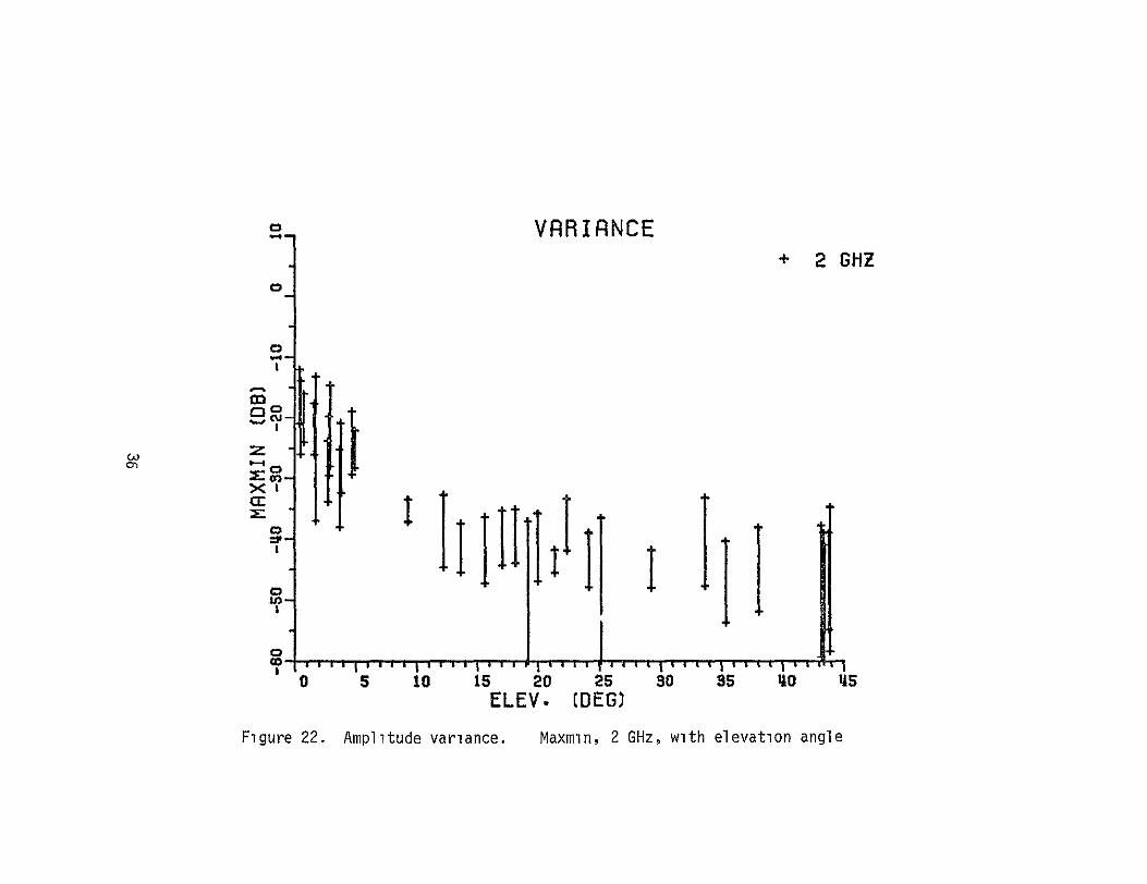
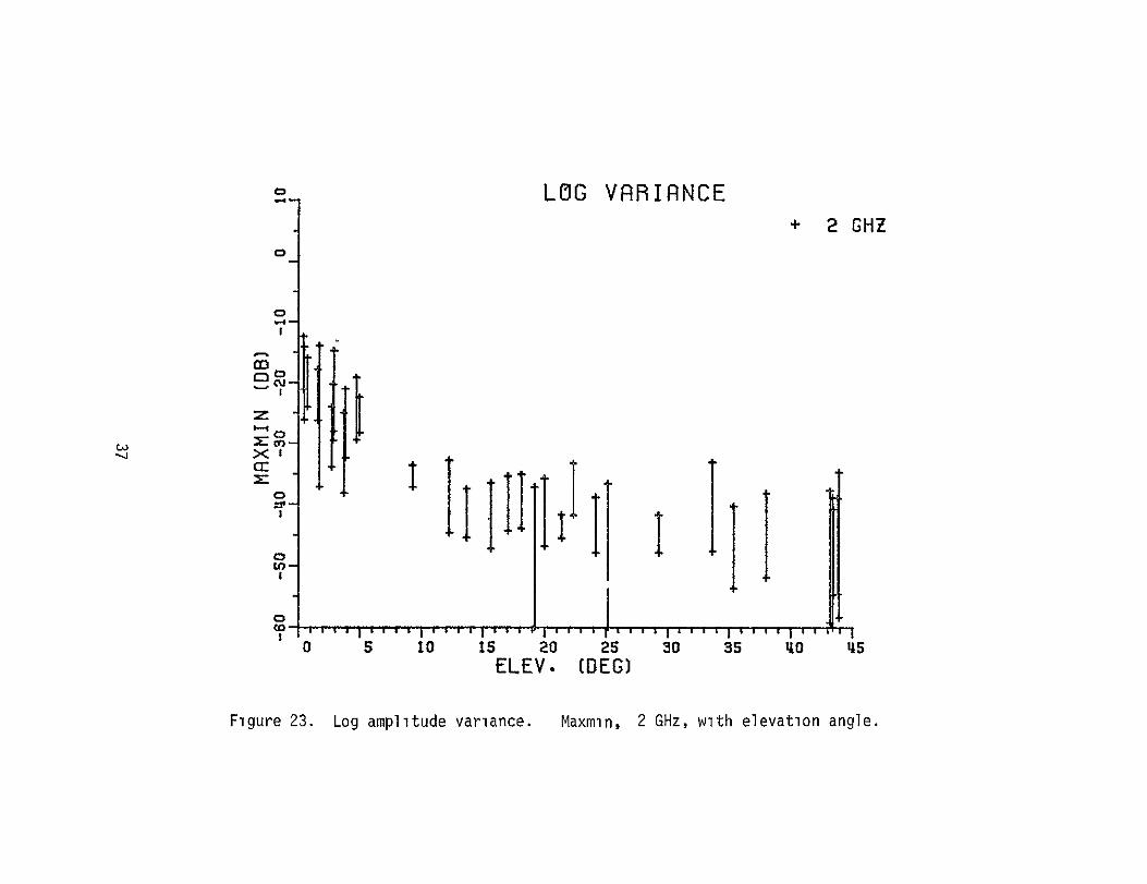
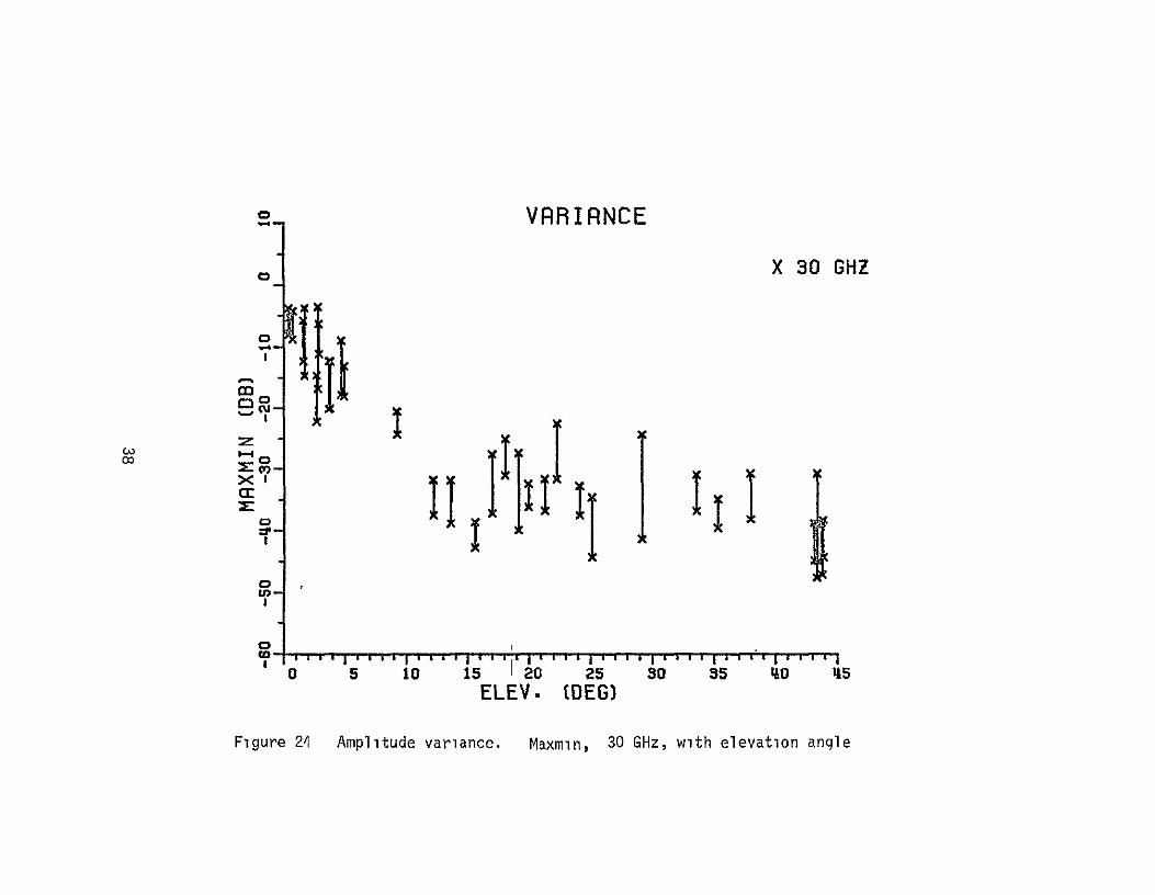
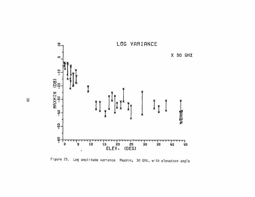
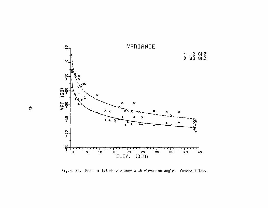
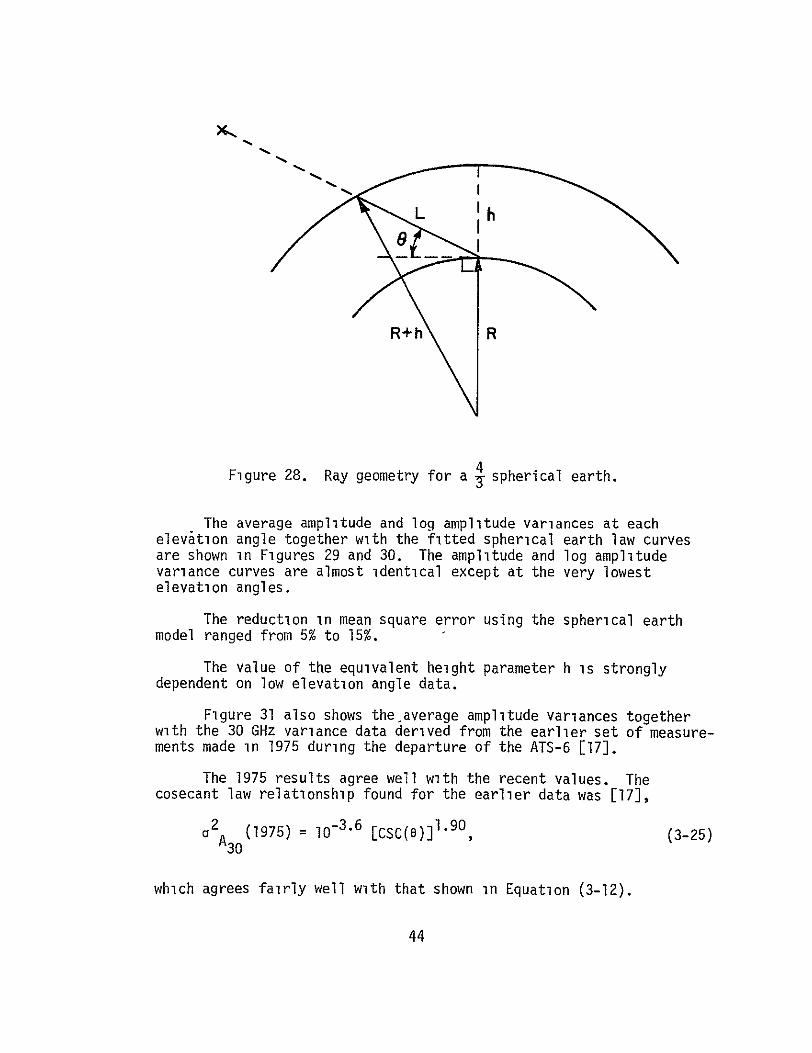
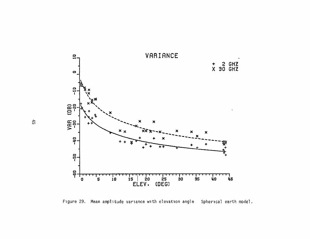
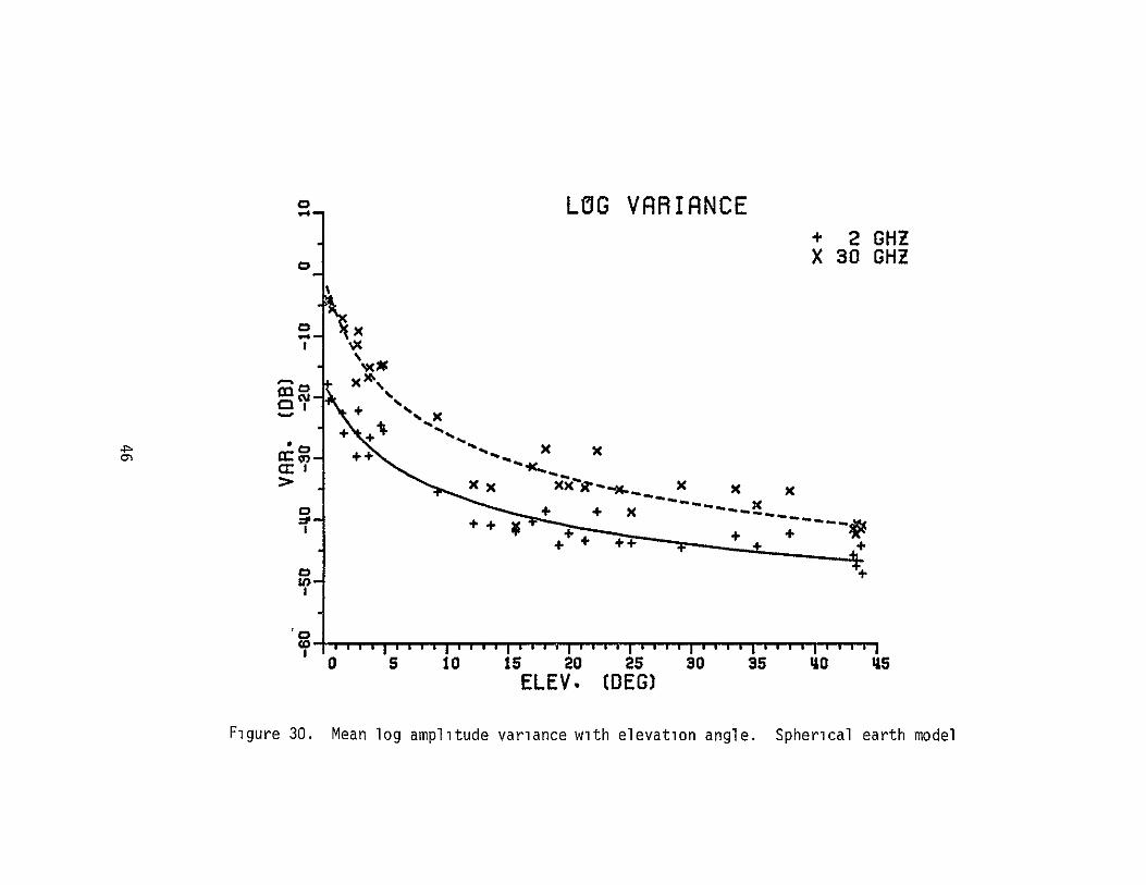
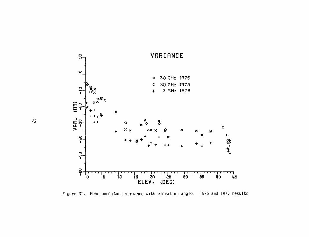
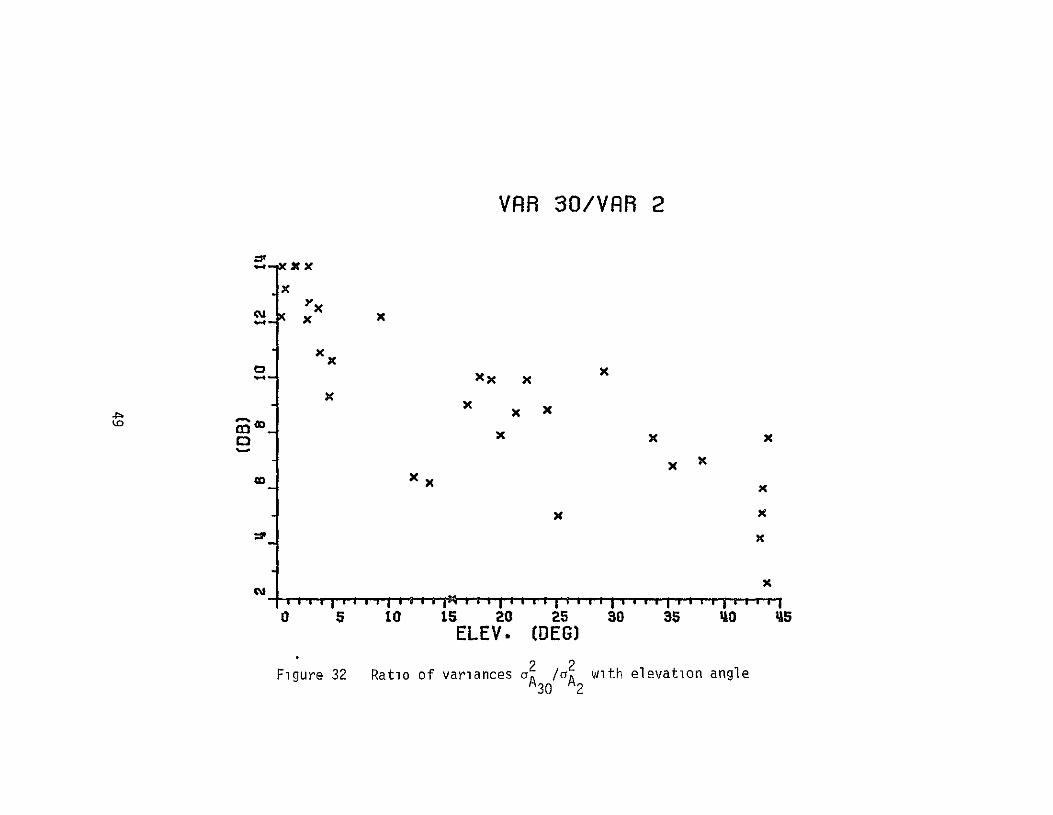
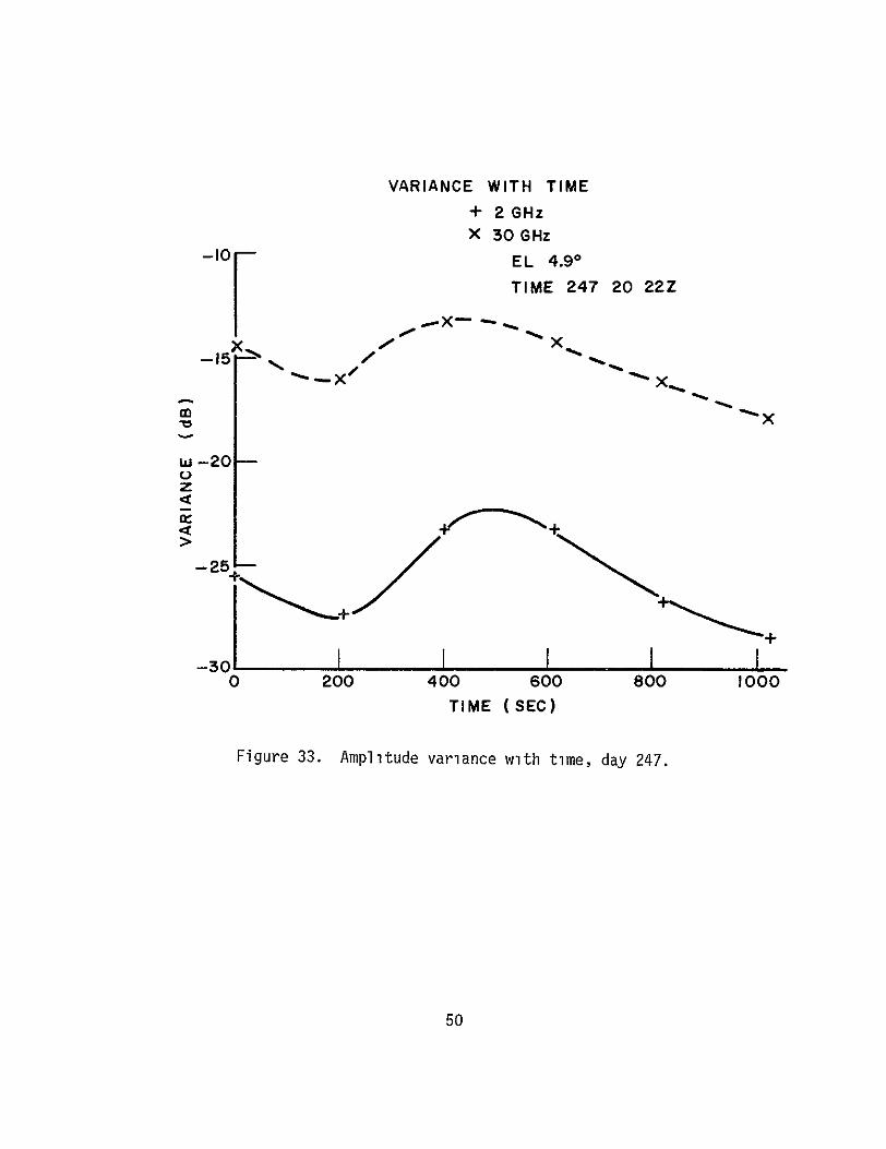
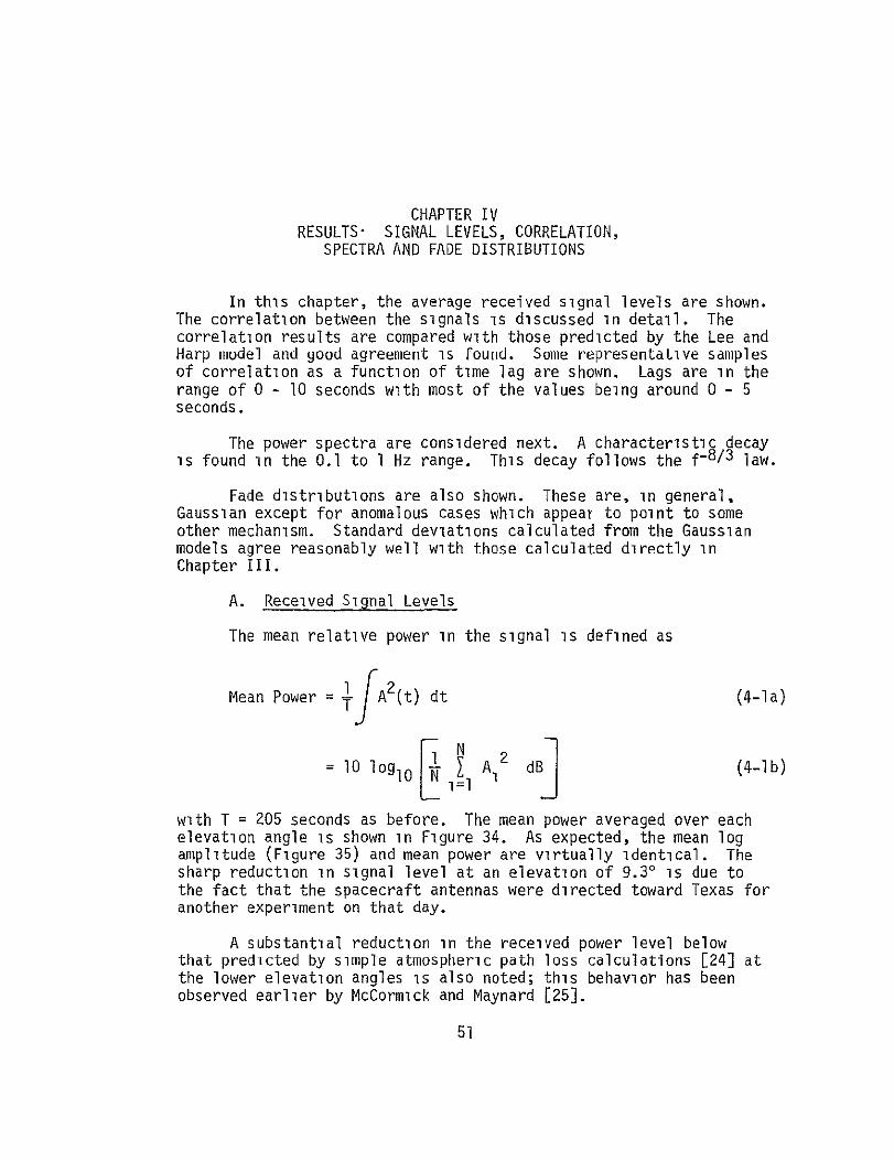
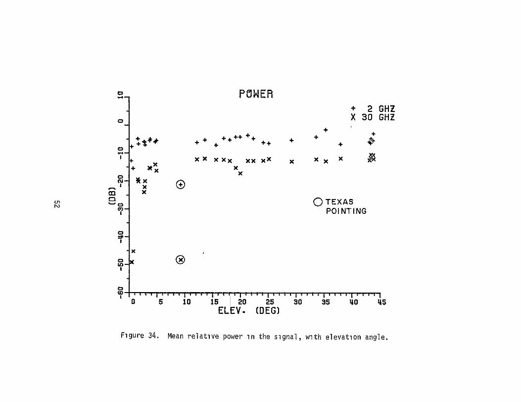
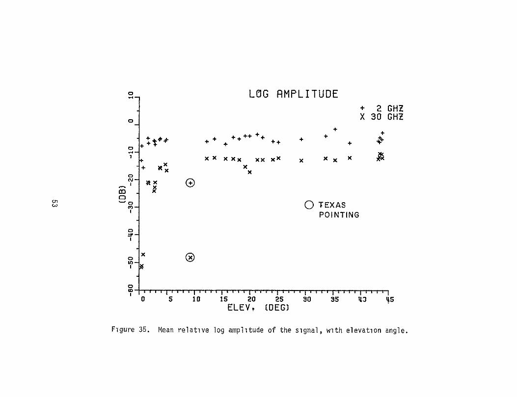
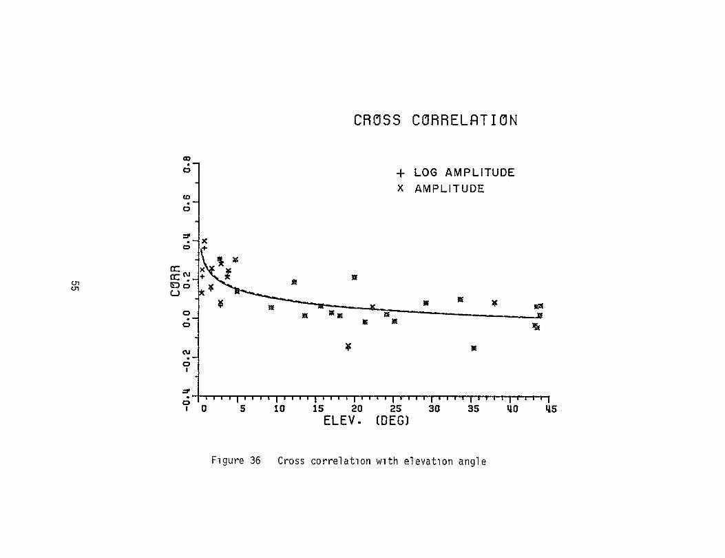
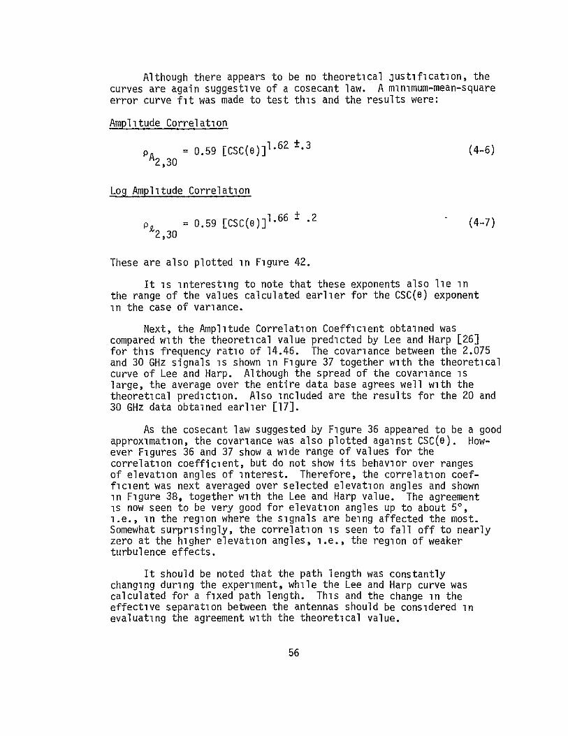
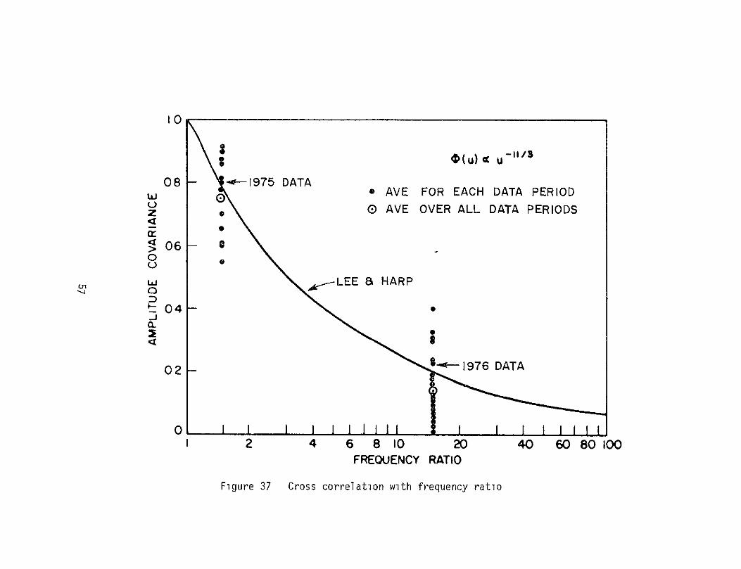
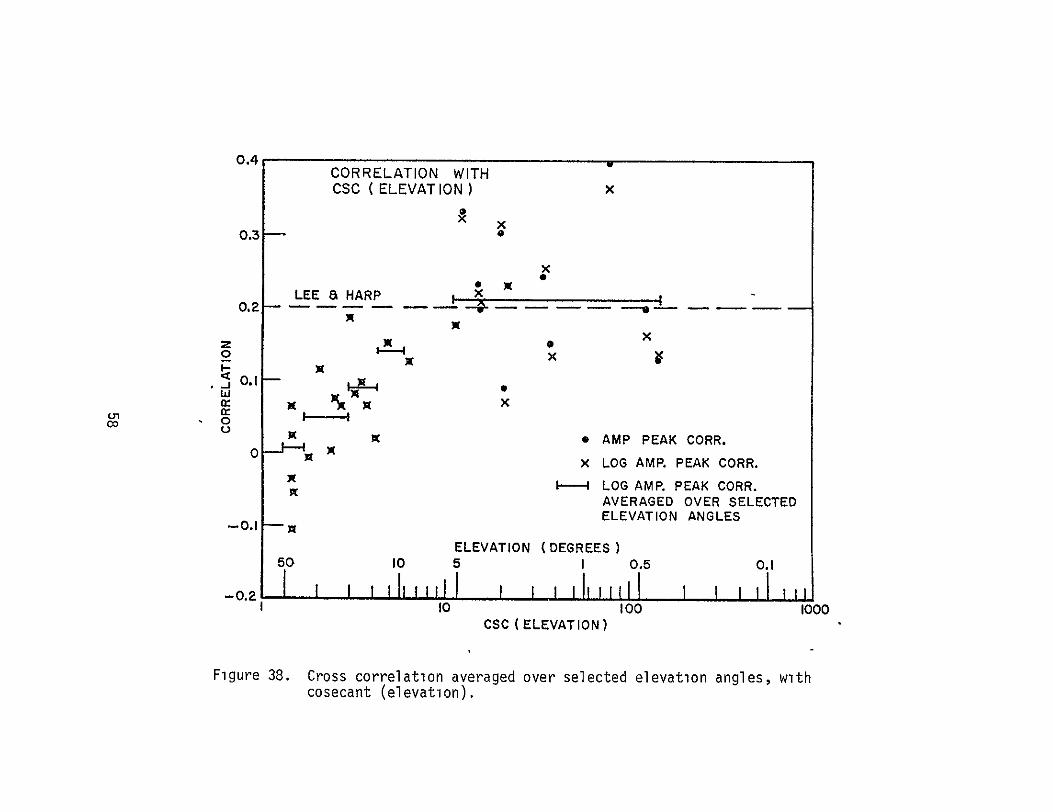
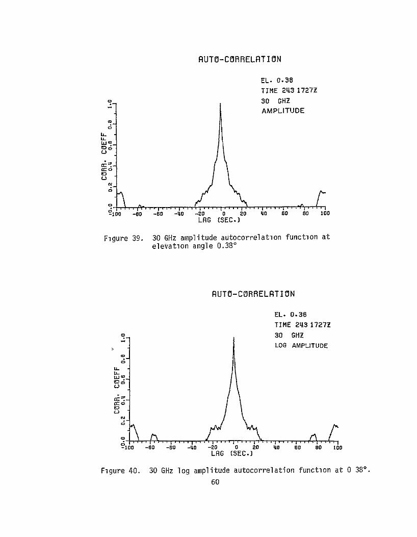
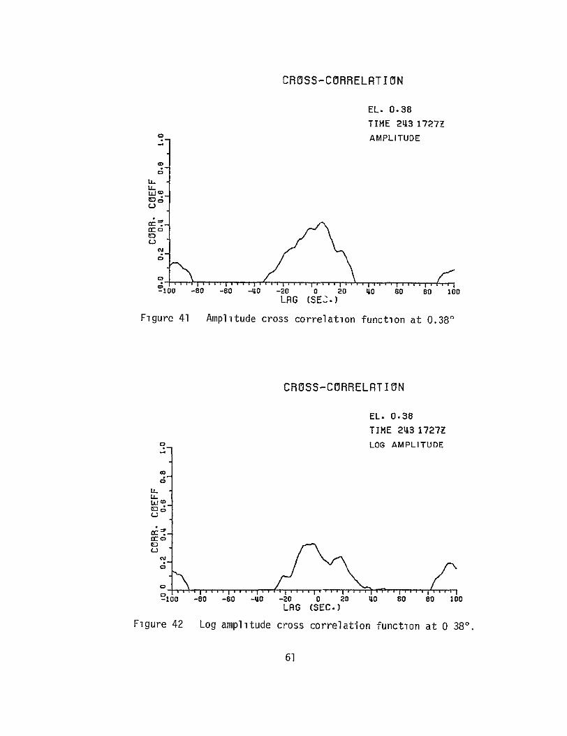
CROSS-CORRELRTION
EL 038
TIME 213 1727 o AMPLITUDE
IL
-
C 4
10o -80 -s0 -40 -20 0 20 40 so so 20D LAG (SE--)
Figure 41 Amplitude cross correlation function at 0380
LU0
L) CROSS-CORRELAITION
EL 038
TIME 243 1727Z
o LOG AMPLITUDE
8shy
-100 -80 -80 -10 -20 0 20 o so 80 100 LRG (SEC)
Figure 42 Log ampltude cross correlation function at 0 380
61
CROSS-CORRELRTION
EL 495
TIME 247 2029Z o AMPLITUDE
UJ
C
tzOil -0 6 -40o -20 rl 20 40 60 80 100LAG (SEC)
Figure 43 Amplitude cross correlation function at 4950
cJ cc
- CROSS-CORRELATION
EL 929
TIME 251 171t4Z
o_ - AMPLITUDE
o -oo -so -60 -w -20 0 20 40 s0 80 100
LAG (bEC)
Figure 44 Amplitude cross correlation function at 9 290
62
CROSS-CORRELATION
EL- 22-31i TIME 263 1839Z
o AMPLITUDE
U-
C
C-
-100 -80 -Be -140 -20 a 20 40 6C) 80 10o LRG (SEC)
Figure 45 Amplitude cross correlation function at 22340
RUTO-CORRELATI ON
EL 113-89
TIME 298 1820-7
o2 GHZ
AMPLITUDE
8shy0
0 -80 -80 -0 -20 0 20 140 0 80 100 LRG (SEC)
Figure 46 2 GHz amplitude auto correlation function at 43890
63
C Spectra
Sample spectra of the received signal are shown in Figures 47 through 53 Corresponding records of received signal will be found in Figures 7 through 28 These spectra all show a characteristic decay with frequency in the range from approximately 01 Hz to 10 Hz The spectra tend to be relatively flat outside that range
The slope of the spectra in the decaying region was measured manually for several samples The results of 12 samples each at 2 GHz and 30 GHz are shown in Table 3
Table 3
SLOPE OF SIGNAL SPECTRA
2 GHz 30 GHz dBdecade dBdecade
MAXIMUM 306 312
MINIMUM 235 200
MEAN 255 268
These results agree closely with a power roll-off relationship of the form f-8 3 or 267 dBdecade This result also agrees with the assumption that a tropospheric turbulence mechanism is producingthe observed scintillations [27]
64
O POWER SPECTRUM
2 GHl RECEIVER EL 038
ai0 TIME 243 1727Z SCU
C
-j LUEDm
0
0
FREQ IN HZ
(a)
OPOWER SPECTRUM
30 GHZ RECEIVER
EL 038 0 TIME 243 1727Z
-C
U
jco
FREQ IN HZ
(b)
Figure 47 Power spectra at 0 380
65
o POWER SPECTRUM
2 GHZ RECEIVER
EL 160 TIME 244 2024Z
=7- N EU
degx
FREQ IN HZ
(a) Cr
U
LI S-Jo o POWER SPECTRUM
~30 GHZ RECEIVER
ccEL 180 wo TIME 244 2024Z
FREQ IN HZ
(b) Figure 48 Power spectra at 1600
66
_ POWER SPECTRUM
2 GHZ RECEIVER
cc L
EL TIME
282 216 2 16Z
-
cc
(a)
U
~POWER SPECTRUM
C IL 30 GHE8RECEIVER
co
UOTIME 246 2 16Z
C
-J
FRE IN HZ
(b)
Figure 49 Power spectra at 2820
67
o POWER SPECTRUM
2 GHZ RECEIVER EL 495
U TIME 247 20292
a
J
LU 0
FREQ IN HZ
(a)
oPOWER SPECTRUM
30 GHZ RECEIVER EL 495
L TIME 247 2029Z
cc - U
a S-
FREQ IN HZ
(b)
Figure 50 Power spectra at 495
68
C POWER SPECTRUM
2 0HZ RECEIVER EL 1811
o TIME 259 1913Z
a 0
m-J
FREQ IN HZ
(a)
o_ POWER SPECTRUM
30 GHZ RECEIVER EL 1811
Uj TIME 259 1913Z
oIm
FREQ IN HZ
(b)
Figure 51 Power spectra at 18 110
69
o POWER SPECTRUM
2 GHZ RECEIVER EL 2234 TIME 263 1842Z
-C
aCr
L)
CD
C
FRED IN HI (a) 0H
oPOWER SPECTRUM
30 GHZ RECEIVER EL 2234 TIME 263 1842Z
-c
m I
FREG IN HZ (b)
Figure 52 Power spectra at 2234
70
b
o POWER SPECTRUM
2 GHZ RECEIVER
EL 4389 TIME 298 1850Z
Cr
C
-J
FREQ IN HZ
Figure 53 Power spectrum at 43890
71
D Fade Distributions
Fade distributions were also studied at several elevation angles averaging about 30000 samples ie 50 minutes each Figures 54 and 55 show the percentage of time a given fade depth was exceeded plotted on a log-normal scale
The curves appear to fit fairly well within each other with increasing elevation However exceptions are clearly seen at 038 and 1600 for both 2 and 30 GHz and at 495 for the 2 GHz signal The reason for the behavior at 495 is not clear at present It should be noted that the 30 GHz fade distribution at this elevation angle does not behave in the same way
The distributions at 2820 are taken to be a representative sample for the higher elevation angle cases and show good fit to straight line approximations indicating that they are Gaussian Even the anomalous distributions show a Gaussian nature over a large portion of their ranges
The fade distributions could in fact be a combination of more than one type of statistic Deviations from the Gaussian curve are prominent for large scintillations Furthermore since the sampling rate is high (10sec) it is possible that the effects of rapid short term scintillations which are believed to be Rayleigh distributed are also being displayed in these distribution curves [28]
Assuming that the dominant long-term statistics at-the higher elevation angles are Gaussian a check was performed at 2820 as follows Let the un-normalized variance be s2 For a log-normal distribution the interval between the 50 and 999 percentile values of the cumulative distribution function - ie 50 and 01 pershycentile values of the fade distribution function - is 31 s[29] For 30 GHz from Figure 55
31 s30 = 86
=27s30
Now from the definition of a2 (Equation (3-6)) we can write that
0 ogloG2 =
dB K1
2zdB
= K110os
72
9999 FADE DISTRIBUTIONS
2 GHz 999 998 -
99 gtt
AA A
ELEVATION (DEG)
98 bull A 0
X 038 160
95 9-0D A o628228 04 A 495
90 x 0 1811 + 1+ 4381
x c0 o X
w 70 x w + E3
x 60shy
lt 50 + 40- 13
350- 0 0
C20 + x
1-0- A3 X x~
ox x 5-+ C X
+ A x X XX
2 I-
+ A
05 a
02- 0
0I 005
001 0 1 5 4 5 6 7 a 9
FADE (d8)
Figure 54 Fade distributions at 2 GHz
73
9999
999
998 -
FADE DISTRIBUTIONS
30 GHz
w w o x
99
98
95
80
A
X
x
ELEVATION (DEG)
038 x 160 0 282 A 495
1811 + 4381
600
650 a
S40 -x
w30-
-20 20
A
A x 0
10-0+D
0+ 0 5-
2--x 5
A30
Abull 0
X
0
S
X X
X OX x
2- A X
02- I A- 0 0 x
021
0010 5 10 15 20 25 30 35 40 45
FADE (d8)
Figure 55 Fade distributions at 30 GHz
74
From Figure 27 average log amplitude variance at 282
2 a ZdB 30 = - 115 dB
-115
s30 = (20 loglo e) 1 010
s30 = 234
This compares favorably with s as calculated from Figure 55
Similarly for 2 GHz at 282 from Figure 54
31 s2 = 23
= 074s2
from Figure 27 and following the same procedure as above
s2 = 045
The discrepancies could be partly due to the fact that the values shown in Figure 27 are calculated for 205 second intervals only and then averaged over each elevation angle These are therefore shortshyterm statistics and would tend to be Rayleigh distributed whereas the distributions in Figures 54 and 55 were calculated over the whole elevation angle directly these tend to be Gaussian Further the deviations from the log-normal curve for strong scintillations would also affect the result
75
CHAPTER V CONCLUSIONS
The results of the experiment are summarized in this chapter
A The Received Signals
The received siqnals show several types of fluctuations
a) Very low elevation angles (less than 40)
(i) Slow rises and fades of tens of dB over periods of tens of minutes
(ii) Faster fluctuations or scintillations with durations of a few minutes or less occurring continuously
(il) Continuous rapid scintillations of a dB or less
(iv) Slow roller-type fading is also seen However the high signal correlation found rules out ground reflection effects (Appendix D)
b) Low elevation angles (40 to 100)
(1) Very slow changes in mean level of a few dB over 30 minutes or more
(ii) Faster scintillations of several dB with periods of a few tens of seconds
(il) Continuous rapid scintillations
c) Medium elevation angles (10 - 44)
(1) Virtually no change in mean level except during precipitation events
(ii) Enhanced scintillations of a few dB for a few minutes are now visible
(iii) Continuous rapid scintillations
Scintillations were observed at all times in clear air and also in the presence of non-precipitating clouds At the highest elevation angles there appears to be a tendency for the scintillations to be enhanced in the presence of non-precipitating cumulus clouds
76
In the following discussion the symbols A and k are used to denote amplitude and log amplitude quantities respectively The symbol V is used to denote either one in general
B Variances
Amplitude and log variances are defined in Equations (3-4) and(3-6)
The range of the variances at any elevation angle exceeded 20 dB at times However the average variances followed a cosecant power law with elevation angle fairly well
Table 4
2 A [CSC(EL)] B
2 GHz 30 GHz
A B A B
10-4 9 12 162 10-4 3 214A 2 plusmn3
-43 a 2 10-49 162 10 220plusmn2 plusmn3
The fairly large error bounds have been introduced to account for the limited data Observations over extended periods under widely varying weather conditions would give a closer estimate The exponents B compare well in their range of error with the theoretical value B = 1833 for Kolmogorov type turbulence
As a refinement a spherical earth model was assumed with a uniform homogeneous atmosphere of effective height h km When this was fitted to the data the results were as follows
77
Table 5
a2 -A LB
L =Ih2 + 2hR + R2 Sin2e - RSine
R = 8479 km 0 = elevation anole
2 GHz 30 GHz
A B hkm A B hkm
10- 6 5 10- 6 4A 187 62 248 61plusmn2 plusmn1 plusmn3 plusmnI
2 10-6 4 187 61 1061 249 45
plusmn2 plusmnIt3
A reduction inmean square error of between 5 to 15 is obtained However in general the much simpler cosecant law
a A [CSC(amp)]B
appears to be quite adequate for elevation angles above 40
The 30 GHz data obtained during the departure of ATS-6 in 1975
agree well with the present data
The ratio of variances a2 1 2 has a mean value of 92 dB
A value of 44 dB was obtained for a2A30l 2A inthe 1975 measureshyments 3
C Received Signal Levels
The relative received signal levels show a strong dependence on elevation angle for elevations less than 5 They are relatively independent of elevation thereafter The drop in signal levels at low elevation angles are much greater than simple path-loss calcushylations predict
78
D Cross Correlations
Cross correlation was evaluated as a function of elevation angle Both the amplitude and log amplitude cross correlations are identical for elevations above 5 Below this angle they diverge slightly The cross correlations appear to follow a cosecant law with an exponent of 161 to 166
The average amplitude correlation was found to agree well with that predicted by Lee and Harp for the frequency ratio of 1446 The 1975 data also show good agreement with the predicted value for a frequency ratio of 15
Representative samples of auto and cross correlation functions with time lag were also shown Cross correlation lag ranged from 0 to about 10 seconds with most of the values in the region of 0 to 5 seconds Significant correlation was not found for lags exceeding 15 seconds
E Power Spectra
The power spectra of the 2 and 30 GHz signals show a characshyteristic decay with freguncy in the region of 01 to 1 Hz The roll-off follows the f- law agreeing with the assumption of tropospheric turbulence as a dominant mechanism in the samples analyzed
F Fade Distributions
Fade distributions were calculated for selected elevation angles The results suggest dominant Gaussian distributions However there is significant deviation from the normal curve for strong scintillations at low elevation angles
Fades in excess of 30 dB at 30 GHz and 7 dB at 2 GHz were observed for 5 of the time at low elevation angles These dropped to 1 dB and 06 dB respectively at 410
G Summary
Microwave signal amplitude scintillation characteristics were studied on earth-space paths for elevation angles varying from 04 to 439 using the ATS-6 satellite Beacon signals at two frequencies 2 GHz and 30 GHz were monitored simultaneously The results are consistent with similar measurements made earlier at 20 and 30 GHz
Variances are modeled well by the cosecant law and by a homoshygeneous spherical earth model with an equivalent height of 6 km Agreement with the Kolmogorov turbulence model is found The mean ratio of the variances is 94 dB
79
The correlation between the two signals was as high as 04 at low elevation angles and follows a cosecant law The average value is close to that predicted by Lee and Harp for the ratio of these frequencies Correlation lags were in the 0 - 5 second range and significant correlation was not found for lags exCeeding 15 seconds The lags may be attributed to wind fields as modeled by Lee and Harp
The power spectra at both 2 and 30 GHz show an f-8 3 roll-off in the 01 to 1 Hz range This agrees with the assumption of tropospheric turbulence as the dominant mechanism
Mean signal levels dropped sharply below predicted values at elevation angles below about 40 Fades exceeded 30 dB and 7 dB at 30 and 2 GHz respectively for 5 of the time at low elevation angles These reduced to less than I dB at an elevation of 410
The long term statistics are Gaussian except for strong scintillations when significant divergence from the Gaussian distribution was found
80
APPENDIX A EDITED TAPE FORMAT
The format of the final edited working digital magnetic tape corrected for receiver calibration characteristics is shown
Packed Tape 48 File Format
File No Day No of Records (1976)
1 243 244 38 2 245 40 3 246 247 100 4 251 254 255 47 5 257 - 263 265 266 165 6 271 18 7 275 277 281 54 8 291 292 294 296 298 70
Packed Tape 48 Record Format
Record Length = 2555 Integer words
words 1-10 = Header Wl = No of words in Record W2 = Day W3 = Hour W4 = Minute W5 = Second W6 = millisecond W7 = Azimuth (milli degrees) W8 = Elevation (milli degrees) W9 = Record Type (10 a 110 sec rate samples) W1O = Data Status
Bit = -Bit 1 = 2 GHz Rec Bit 2 = 30 GHz Rec
If receiver is on and data is usable the
corresponding bit = 1
Words 11 - 2555
Wll - W2058 max = Packed data words
in 01 dB Bits 0 - 11 2 GHz below reference IBits 12 -23 30 GHz
Remaining words are unused
81
APPENDIX B TABLE OF USEFUL DATA PERIODS
The data recorded during the experiment were edited by eliminating periods of equipment adjustment antenna peaking or adjustment and data corrupted by ground reflections at elevation angles below 038
B-I This section of the Appendix shows the periods duringwhich the data was considered usable after editing
a) Column 1
Entry number
b) Column 234
Time of day (Days Hours Minutes) Greenwich Mean Time
c) Column 56
Nominal Azimuth and Elevation angles in degrees
d) Column 78
These give the external additional attenuators in the receiver which were not directlyrecorded by the data recording system
e) Column 9
The status of the data is given in this column as an octal number as shown below
Bit no 2 1 0
Status I
Receiver 30 GHz 2 GHz 360 MHz
An acceptable data period is indicated by the corresponding bit being set to 1
82
NO OAY HOUR MIN A1 M ELEV 30 GHZ e GHZ STAT (nul (DEG) (DB) (DIR)
1 e6 10 0710l - A 14
e43 4 0 97I0 -4c4 1 1 6 37 24 -474f 6P 6 6
4 4 1 97 4F 3 o b 1b 24o4a 974F 6p 0 4 6 446 1J )2 9746 6p 1 0 7 246 19 18 97b7 45 0 6 4
8 )
a43 3L
3 it)
9763 97ol
47
47 C 0
8 b
7 r
10 2115 2L 17 9761 47 0 7
11 e45lfl -A 97b3 47 1 1 0 oe e44 bU 9eQ19 4 e 7
16 244 6 0 9819 74 0 n 5 14 244 9 50 9860 99 L 0 5
U0lb lamp
-244
i ) 1n
a 9
9AO 9830
99
99 3 b
0 1
1 4
j7 241 10 A6 9aoO 97 5 04 la 244 1ii 57 q81 5 1 1008 10 0 5
39 244 1x 30 9837 135 le 14 20 e44 IB 50 9850 154 10 3 4
244 0 I 98D9 lobO I0 2 6
22 44 41 0 959 lbO lu 2 I 26 24
45 445
1 2
54 8
9895 9P95
17017o 1030 22 27 2b e-45 6 1 9 g 95FT L7nIC 2 5
NO UAY HOUR MIN AZi M ELLV 60 GFl7 wbi$Z STAT (fLG) (DEG) (UP) (U )
4b 4 56 9913 181 1L 2 4 eL45 U 85 9913 161 0 2 5 e45 7 30 9p2 196 10 2 5
29 e45 9 20 99e2 196 10 2 4 3U =45 9 4u 99e7 211 ILI 2 5 31 11 4b50 90e7 211 16 2 U 52 24b 12 O 9941 21 3 I 5 36 245 13 15 9931 P63 i( 2 4 -4 c45
45 It 14
0 3Q
9961 99 54
263 247
IG IC
2
4 4
o6 d45 16 30 3 9 22b7 10 2 4 37 245 lb M1 9q47 b6 IC 2 4 38 245 z 6 9b6 271 10 2 6 35 40
45 e46
21 1
U 54
9b6 9994
71 26p
IC 10
2 2
0 7
41 246 0 9994 282 10 2 5 12 e46 4 U 100116 p6C 10 2 5 41 246 5 6 10006 28q 10 2 7 L4 246 b U 30f06 289 10 2 fl I b 6 17 4 10040 72 10 2 6 46 246 IS 4 10040 37 10 4 u7 246 19 U 3Lin Q $7 1 2 4 48 246 2C 4 10054 --82 I0 2 6
ee46 21 U 1On54 Ab2 10 2 4 50 a46 21 30 lO0Dt 6b2 10 2 0
NO UAY HOUR IIN AZI fuI ELEV 60 GIZ 2 bHZ STAT (DEG) (PLG) (DP) (Or)
51 47 b 9 10136 474 22 2 6 52 247 16 10153 474 22 2 4 So d47 17 U 30133 483 22 2 4 594 247 je 54 10147 491 22 2 5 95 e4 7 0 19 101 bE 495 22 2 7 5( 247 21 2 101b59 495 22 2 0 57 248 16 55 10268 594 22 2 5 58 248 19 U 10247 602 22 2 0 59 251 j7 4 10545 92c) 1) 7 60 ebl 17 2U 10545 929 2 0 0 61 e54 11 6 10850 1222 22 0 7 62 254 12 95 1P50 12e2 22 6 66 e 32 n UPSbU 1222 amp2 0 7 64 254 12 30 XOU50 1222 2 0 0 65 e55 15 34 10a67 16b3 22 0 7 66 255 16 25 10q67 163 22 0 0 67 e57 23 5 ltf 156 22 0 7 f6 eb7 14 U 111L 1t65 22 0 o 69 258 36 11316 17o4 22 0 6
r70 258 19 50 11316 1704 22 0 0 71 259 18 31 l11o2 1811 22 0 72 259 19 30 31462 1811 2a 0 0 76 260 19 29 11550 1918 22 0 6 74 260 19 26 11551 1918 22 0 4 7t 260 19 27 11550 1918 22 2 6
N10 DAY HOUR MIN AziM1 ELEV O GH2 2 6H7 STAT ( Lu ( Lu) (OH) (UU)
76 260 19 51 11 0 19018 22 2 0 77 261 i6 31 1r453 1998 22 7b e61 IN 31 111453 1998 2 2 u 79 262 2 118G3 r216 22 2 E bu 61 20 59 l1v 263 0 Pl 266 1A 19 1117 2264 22 2E 82 263 19 40 llq17 2234 1 2
86 e65 49 12a V 2416 P2 2 6
84 265 14 30 12158 2416 2 2 0 pound5 2E6 i1 1 122~v a 3t4 dc -
86 e7
266 266
16 -14
37 1
1228Q 12LP39
2r14 5o1
22 2
2 U
86 266 14 30 1226 2514 e2 0 8 271 4 52 12922 2923 22 0 6 9 e7 Q 1 2 94e 2SZ3 22 0 0 91 e71 4 66 1C942 2c3 22 6 92 eTi 5 51 1292 2926 22 2 0 96 e5 17 06 166i0 33br 22 2 6 94 475 18 50 ii0 53b 22 2 0 95 e77 2U 52 13972 653 2 2 96 277 21 56 15972 3566 22 P 0 q7 281 1 )I 144kj ULu2 22 2 6 9 t 281 1 41 14641 5 02 2e 2 0 99 291 2U b 14764 4aiq 22 2 6
IOU eql 21 0 167a 4119 22 2 U
NO t AY HOUR MIN AZIN ELEV 30 GHZ 2 GHZ STAT (uEb) (WEG) (08) (JB)
101 e92 l 5 169 16 44 22 6 102 292 19 15 16076 43Q44 22 2 0 106 94 C 55 17278 63A 22 b 14 2994 6 30 1727P 413A 22 2 0
105 296 134 27n414 4381 2 C 1o6 96 15 0 1784 4361 22 2 0 In d98 1e 20 18342 4389 22 2 6 lob 98 19 0 18342 43a9 22 2 0
B-2 The durations of the data periods used in the calculations in this report are given below
Elevation (degrees)
038 048 074 160 170 271 282 289 372 382 474 495
929 1222 1363 1565
Duration (minutes)
32 19 20 46 71 57 61 57 60 56 52 42
16 84 54 57
Elevation (degrees)
1704 1811 1918 1998 2135 2234 2416 2514 2923 3365 3536 3802
4319 4344 4358 4381 4389
Duration (minutes)
54 59 81 59 57 71 41 50 57 57 57 56
52 57 35 66 40
OF POOR QUPLrfORIG19M FAOt 1S
88
APPENDIX C COMMENTS ON LOG AND AMPLITUDE VARIANCE
Expanding the definition of log variance (Equation (3-6))
N 12NN2 1 1a = iL-- I~N 1 kJ KIN i=1( l 22
2 1 N a
= (120 log101 0a 20 lOgio (C-1)
K2N 11 a0 NJ 2 1091 ) 10
but
a a lglO a9 l - + lg0 ashy
0 a o
N a2 202 N O - 1 1oq 0 -- + loK10 To - logl - +10
K1IN i=1(I a o yl
a09lt2N aya
KaN1 20 10
20 Y2 1
1090 logoeK =a I a
Kl = lOg0 e loge
a a
2 a N
a_Y (20 loglo -_1I N I loge l 2 2 (20 logloe)2
(20 logloe) I a j=1 a
89
For small scintillations a
a 1
lo e = - Jrl
Also
2 1 Cf
ala
(a 1 1
a) (C-2)
2= N a
ao
2 N (a shy T)2
2 - 02(-3)
2 a2 for small scintillations
The computed results show excellent agreement even at low elevation angles (ie large scintillations)
Further Fried has shown [30] from energy considerations that
a2p _-T (C-4)
(This result has been adapted to be consistent with the definitions used in this study)
90
0
Now Z shows a sharp drop at low elevat~o9 angles It seen n Figure 56 where the numerical values of K1 a z(NB not pounddB
are plotted that this behavior is in fact reflected
The observations are therefore consistent However the reason for the sharp knee in the mean levels is yet to be determined
LOG-VRRIRNCE
+ 2 GHz
x 30 GHz
x2 IX)2
ci X X
CD
x
+
5 10 15 20 25 30 35 40 45 ELEV (DEG)
Figure 56 Log amplitude variance (numeric)
91
APPENDIX D RECEIVED SIGNALS AT LOW ELEVATION ANGLES
AND MULTIPATH EFFECTS
The mechanism which causes the amplitude scintillations may be regarded as being either refractive or multipath in nature Low two-frequency correlation would be expected if multipath were the dominant factor because an arbitrary differential path length cannot produce simultaneous subtractive or additive phasing at the two wavelengths employed as shown below [17]
Subtractive multipath phasing will occur at a wavelength of X1 if the difference between the two path lengths satisfy
AL = (2n+l) -7 n = O 2
Similarly at a second wavelength X2
AL = (2m+l) 2p m = 0 1 2
Therefore
(2n+l)A 1 = (2m+l)A 2
But in general
A I = PA2 where P is an arbitrary number
So that
P(2n+l) = 2m+l (D-1)
For example the 1975 measurements were performed simultaneously at 20 and 30 GHz therefore P = 32 Then
3 (2n+l) = 2m+l
or 3(2n+l) = 2(2m+l) (D-2)
However the left side of Equation (D-2) is odd and the right side is even Therefore simultaneous fading due to simple multishypath propagation cannot occur This result contradicts the very high correlations observed between the 20 and 30 GHz signal fluctuations Thus one is forced to conclude that the observed fluctuations are not a result of a simple multipath mechanism
92
APPENDIX E SUMMARY OF DEFINITIONS
a(t) is a positive real signal amplitude a are discrete samples of a(t) at equal intervals over a time interval T a(t) has been corrected for receiver nonlinearities The relative amplitudeis defined to be
a A =- I I a0
and the relative log amplitude as
20 logO ashy=
where a0 is an arbitrary constant
93
AMPLITUDE LOG AMPLITUDE RELATIONSHIP FORSMALL SCINTILLATIONS
= _ A(t) dt = fT1 (t) dt
MEAN JT d z J T N t T 20 loglo
1= 1 L1=1
MEAN TOTAL POWER I JA2(t) t (MEAN SQUARE) N 2 A vdBz
N i1I
VARIANCE ~ (NORMALIZED TO DC POWER)
2 AT
1jf A(t+i2 A N
dt 2 1 T
Wtd NaAC
2-22
NA 1 1 KNK~I 1lN1=
AMPLITUDE LOG AMPLITUDE
CORRELATION
COEFFICIENT
12 --I (Am (t)-l)(A2 (t+T)-T 2 )dt
PA(t)T Al- O 0A1 A1I[2
(A 2- A-I2 I (A (A2 A2 )
1N=l2 0= A1 A2
2 1 z(t)-T( t+r)-12 )dt
f 2K1l 2
1I2
N ( lI- -I)( 21+j- 2) 1 )
K1N 1=] lP2
RELATIONSHIP FOR SMALL SCINTILLATIONS
PA12 v 2
K 20 logloe T = j T IT
REFERENCES
[1] L Cuccia W Quan and C Hellman Above 10 GHz Satcom Bands Spur New Earth Terminal Development Microwave System News March 1977 p 3738
[2] L Cuccia et al Op Cit p 46-50
[3] D E Kerr Propagation of Short Radio Waves McGraw Hill 1964
[4] B R Bean and E J Dutton Radio Meteorology Dover 1968
[5] D C Livingston The Physics of Microwave Propagation Prentice Hall 1970
[6] Propagation Factors in Space Communications AGARD Conference Proceedings No 3 W J Mackay and Co 1967
[7] P David and J Voge Propagation of Radio Waves Pergamon Press 1969
[8] Communications Satellite Corporation COMSAT Technical Review Vol 3 No 1 to Vol 5 No 2
[9] E V Appleton URSI Proceedings Washington 1927
[10] E H Whitney and S Basu The Effect of lonosphereic Scintillation on VHFUHF satellite Communications Radio Science Vol 12 No 1 1977 p 123-133
[11] Aarons et al Radio Astronomy Measurements at VHF and Microwaves Proceedings IRE January 1958 p 325-333
[12] L A Hoffman et al Propagation Observations at 32 Millishymeters Proceedings IEEE Vol 54 No 4 April 1966
[13] L J Ippolito Effects of Precipitation on 153 and 3165 GHz Earth-Space Transmission With the ATS-V Satellite Proceedings IEEE Vol 59 No 2 1971
[14] L J Ippolito ATS-6 Millimeter WaVe Propaqation and Communishycations Experiments at 20 and 30 GHz IEEE Transactions Vol AES-ll No 6 1975
[15] Goddard Space Flight Center ATS-F and -G Data Book September 1972 p A39-A42
96
[16] D B Hodge and D M Theobold Scintillations Observed on the ATS-6 20 and 30 GHz Downlinks URSIUSNC meeting Boulder Colorado October 1975
[17] D B Hodge D M Theobold and R C Taylor ATS-6 Millimeter Wavelength Propagation Experiment Report 3863-6 January 1976 The Ohio State University ElectroScience Laboratory Department of Electrical Engineerng prepared under Contract NAS5-21983 For NASA Goddard
[18] V I Tatarski Wave Propagation in a Turbulent Medium Israel Program for Scientific Translation Jerusalem 1971
[19] R F F11ipowski and E I Muehldorf Space Communication Systems Prentice Hall 1965
[20] G N Krassner Introduction to Space Communication Systems Chapter 4 McGraw Hill 1964
[21] D M Theobold and D B Hodge ATS-6 Millimeter Wavelength Propagation Experiment Report 3863-4 April 1975 The Ohio State University ElectroScience Laboratory Department of Electrical Engineering prepared under Contract NAS5-21983 for NASA Goddard
[22] B H Briggs and I A Parkin On The Variation of Radio Star and Satellite Scintillations with Zenith Angle J Atmos Terr Phys 25 p 339-366
[23] A Kolmogorov Turbulence Classic Papers on Statistical Theory S K Friedlander and L Topper Eds New York Interscience 1961 p 151
[24] A Benoit Signal Attenuation Due to Neutral Oxygen and Water Vapor Rain and Clouds The Microwave Journal November 1968 p 73-80
[25] K S McCormick and L A Maynard Measurements of SHF Tropospheric Fading Along Earth-Space Paths at Low Elevation Angles Electronics Letters Vol 8 1972 p 274
[26] R W Lee and J C Harp Weak Scattering in Random Media with Applications to Remote Probing Proc IEEE Vol 57 1969 p 375-406
[27] R S Lawrence and J W Strohbehn ASurvey of Clear Air Propagation Effects Relevent to Optical Communications Proc IEEE Vol 58 No 10 October 1970 pp 15371538
97
[28] P F Panter Com unication Systems Design McGraw Hill 1972
pp 347-358
[29] P F Panter Op Cit p 355
[30] D L Fried Optical Resolution Through a Randomly Inhomoshygeneous Medium for Very Long and Very Short Exposures J Opt Soc Am 56 October 1966 pp 1372-1379
98
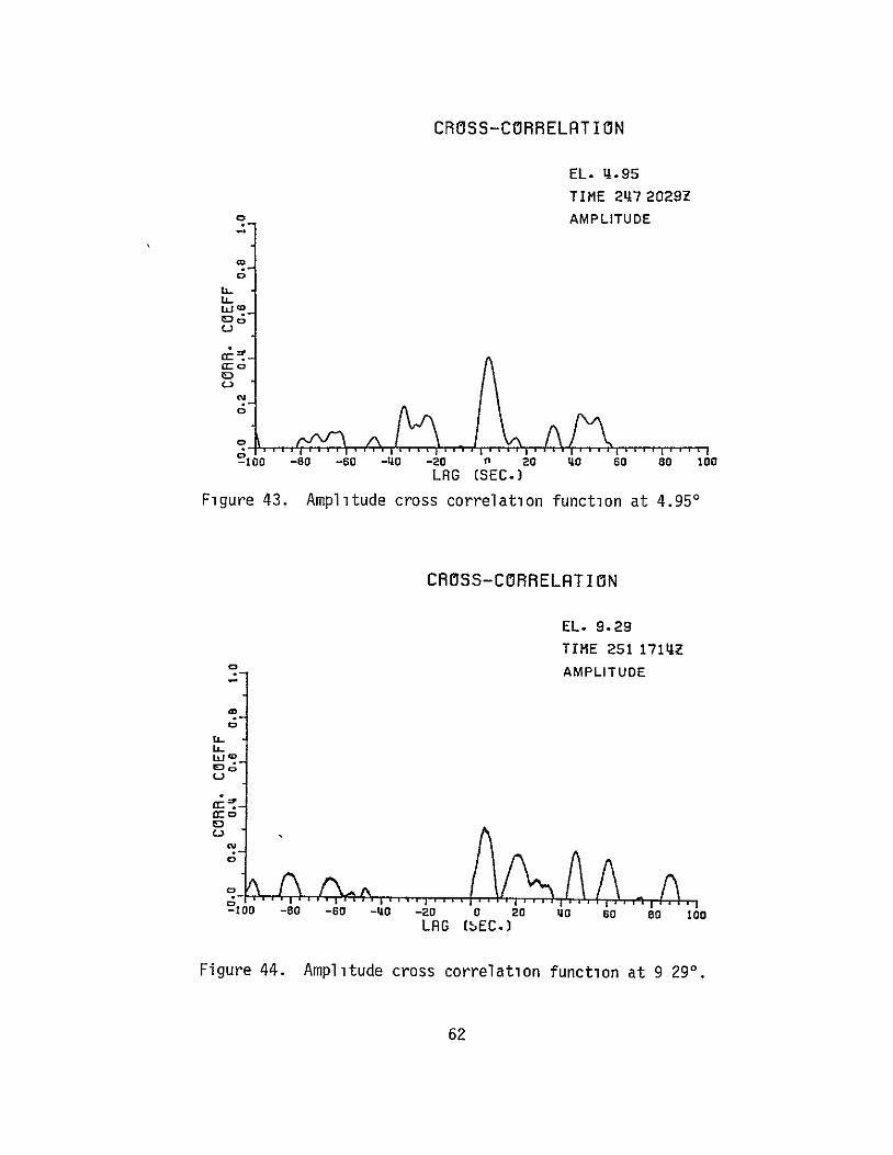
CROSS-CORRELRTION
EL 495
TIME 247 2029Z o AMPLITUDE
UJ
C
tzOil -0 6 -40o -20 rl 20 40 60 80 100LAG (SEC)
Figure 43 Amplitude cross correlation function at 4950
cJ cc
- CROSS-CORRELATION
EL 929
TIME 251 171t4Z
o_ - AMPLITUDE
o -oo -so -60 -w -20 0 20 40 s0 80 100
LAG (bEC)
Figure 44 Amplitude cross correlation function at 9 290
62
CROSS-CORRELATION
EL- 22-31i TIME 263 1839Z
o AMPLITUDE
U-
C
C-
-100 -80 -Be -140 -20 a 20 40 6C) 80 10o LRG (SEC)
Figure 45 Amplitude cross correlation function at 22340
RUTO-CORRELATI ON
EL 113-89
TIME 298 1820-7
o2 GHZ
AMPLITUDE
8shy0
0 -80 -80 -0 -20 0 20 140 0 80 100 LRG (SEC)
Figure 46 2 GHz amplitude auto correlation function at 43890
63
C Spectra
Sample spectra of the received signal are shown in Figures 47 through 53 Corresponding records of received signal will be found in Figures 7 through 28 These spectra all show a characteristic decay with frequency in the range from approximately 01 Hz to 10 Hz The spectra tend to be relatively flat outside that range
The slope of the spectra in the decaying region was measured manually for several samples The results of 12 samples each at 2 GHz and 30 GHz are shown in Table 3
Table 3
SLOPE OF SIGNAL SPECTRA
2 GHz 30 GHz dBdecade dBdecade
MAXIMUM 306 312
MINIMUM 235 200
MEAN 255 268
These results agree closely with a power roll-off relationship of the form f-8 3 or 267 dBdecade This result also agrees with the assumption that a tropospheric turbulence mechanism is producingthe observed scintillations [27]
64
O POWER SPECTRUM
2 GHl RECEIVER EL 038
ai0 TIME 243 1727Z SCU
C
-j LUEDm
0
0
FREQ IN HZ
(a)
OPOWER SPECTRUM
30 GHZ RECEIVER
EL 038 0 TIME 243 1727Z
-C
U
jco
FREQ IN HZ
(b)
Figure 47 Power spectra at 0 380
65
o POWER SPECTRUM
2 GHZ RECEIVER
EL 160 TIME 244 2024Z
=7- N EU
degx
FREQ IN HZ
(a) Cr
U
LI S-Jo o POWER SPECTRUM
~30 GHZ RECEIVER
ccEL 180 wo TIME 244 2024Z
FREQ IN HZ
(b) Figure 48 Power spectra at 1600
66
_ POWER SPECTRUM
2 GHZ RECEIVER
cc L
EL TIME
282 216 2 16Z
-
cc
(a)
U
~POWER SPECTRUM
C IL 30 GHE8RECEIVER
co
UOTIME 246 2 16Z
C
-J
FRE IN HZ
(b)
Figure 49 Power spectra at 2820
67
o POWER SPECTRUM
2 GHZ RECEIVER EL 495
U TIME 247 20292
a
J
LU 0
FREQ IN HZ
(a)
oPOWER SPECTRUM
30 GHZ RECEIVER EL 495
L TIME 247 2029Z
cc - U
a S-
FREQ IN HZ
(b)
Figure 50 Power spectra at 495
68
C POWER SPECTRUM
2 0HZ RECEIVER EL 1811
o TIME 259 1913Z
a 0
m-J
FREQ IN HZ
(a)
o_ POWER SPECTRUM
30 GHZ RECEIVER EL 1811
Uj TIME 259 1913Z
oIm
FREQ IN HZ
(b)
Figure 51 Power spectra at 18 110
69
o POWER SPECTRUM
2 GHZ RECEIVER EL 2234 TIME 263 1842Z
-C
aCr
L)
CD
C
FRED IN HI (a) 0H
oPOWER SPECTRUM
30 GHZ RECEIVER EL 2234 TIME 263 1842Z
-c
m I
FREG IN HZ (b)
Figure 52 Power spectra at 2234
70
b
o POWER SPECTRUM
2 GHZ RECEIVER
EL 4389 TIME 298 1850Z
Cr
C
-J
FREQ IN HZ
Figure 53 Power spectrum at 43890
71
D Fade Distributions
Fade distributions were also studied at several elevation angles averaging about 30000 samples ie 50 minutes each Figures 54 and 55 show the percentage of time a given fade depth was exceeded plotted on a log-normal scale
The curves appear to fit fairly well within each other with increasing elevation However exceptions are clearly seen at 038 and 1600 for both 2 and 30 GHz and at 495 for the 2 GHz signal The reason for the behavior at 495 is not clear at present It should be noted that the 30 GHz fade distribution at this elevation angle does not behave in the same way
The distributions at 2820 are taken to be a representative sample for the higher elevation angle cases and show good fit to straight line approximations indicating that they are Gaussian Even the anomalous distributions show a Gaussian nature over a large portion of their ranges
The fade distributions could in fact be a combination of more than one type of statistic Deviations from the Gaussian curve are prominent for large scintillations Furthermore since the sampling rate is high (10sec) it is possible that the effects of rapid short term scintillations which are believed to be Rayleigh distributed are also being displayed in these distribution curves [28]
Assuming that the dominant long-term statistics at-the higher elevation angles are Gaussian a check was performed at 2820 as follows Let the un-normalized variance be s2 For a log-normal distribution the interval between the 50 and 999 percentile values of the cumulative distribution function - ie 50 and 01 pershycentile values of the fade distribution function - is 31 s[29] For 30 GHz from Figure 55
31 s30 = 86
=27s30
Now from the definition of a2 (Equation (3-6)) we can write that
0 ogloG2 =
dB K1
2zdB
= K110os
72
9999 FADE DISTRIBUTIONS
2 GHz 999 998 -
99 gtt
AA A
ELEVATION (DEG)
98 bull A 0
X 038 160
95 9-0D A o628228 04 A 495
90 x 0 1811 + 1+ 4381
x c0 o X
w 70 x w + E3
x 60shy
lt 50 + 40- 13
350- 0 0
C20 + x
1-0- A3 X x~
ox x 5-+ C X
+ A x X XX
2 I-
+ A
05 a
02- 0
0I 005
001 0 1 5 4 5 6 7 a 9
FADE (d8)
Figure 54 Fade distributions at 2 GHz
73
9999
999
998 -
FADE DISTRIBUTIONS
30 GHz
w w o x
99
98
95
80
A
X
x
ELEVATION (DEG)
038 x 160 0 282 A 495
1811 + 4381
600
650 a
S40 -x
w30-
-20 20
A
A x 0
10-0+D
0+ 0 5-
2--x 5
A30
Abull 0
X
0
S
X X
X OX x
2- A X
02- I A- 0 0 x
021
0010 5 10 15 20 25 30 35 40 45
FADE (d8)
Figure 55 Fade distributions at 30 GHz
74
From Figure 27 average log amplitude variance at 282
2 a ZdB 30 = - 115 dB
-115
s30 = (20 loglo e) 1 010
s30 = 234
This compares favorably with s as calculated from Figure 55
Similarly for 2 GHz at 282 from Figure 54
31 s2 = 23
= 074s2
from Figure 27 and following the same procedure as above
s2 = 045
The discrepancies could be partly due to the fact that the values shown in Figure 27 are calculated for 205 second intervals only and then averaged over each elevation angle These are therefore shortshyterm statistics and would tend to be Rayleigh distributed whereas the distributions in Figures 54 and 55 were calculated over the whole elevation angle directly these tend to be Gaussian Further the deviations from the log-normal curve for strong scintillations would also affect the result
75
CHAPTER V CONCLUSIONS
The results of the experiment are summarized in this chapter
A The Received Signals
The received siqnals show several types of fluctuations
a) Very low elevation angles (less than 40)
(i) Slow rises and fades of tens of dB over periods of tens of minutes
(ii) Faster fluctuations or scintillations with durations of a few minutes or less occurring continuously
(il) Continuous rapid scintillations of a dB or less
(iv) Slow roller-type fading is also seen However the high signal correlation found rules out ground reflection effects (Appendix D)
b) Low elevation angles (40 to 100)
(1) Very slow changes in mean level of a few dB over 30 minutes or more
(ii) Faster scintillations of several dB with periods of a few tens of seconds
(il) Continuous rapid scintillations
c) Medium elevation angles (10 - 44)
(1) Virtually no change in mean level except during precipitation events
(ii) Enhanced scintillations of a few dB for a few minutes are now visible
(iii) Continuous rapid scintillations
Scintillations were observed at all times in clear air and also in the presence of non-precipitating clouds At the highest elevation angles there appears to be a tendency for the scintillations to be enhanced in the presence of non-precipitating cumulus clouds
76
In the following discussion the symbols A and k are used to denote amplitude and log amplitude quantities respectively The symbol V is used to denote either one in general
B Variances
Amplitude and log variances are defined in Equations (3-4) and(3-6)
The range of the variances at any elevation angle exceeded 20 dB at times However the average variances followed a cosecant power law with elevation angle fairly well
Table 4
2 A [CSC(EL)] B
2 GHz 30 GHz
A B A B
10-4 9 12 162 10-4 3 214A 2 plusmn3
-43 a 2 10-49 162 10 220plusmn2 plusmn3
The fairly large error bounds have been introduced to account for the limited data Observations over extended periods under widely varying weather conditions would give a closer estimate The exponents B compare well in their range of error with the theoretical value B = 1833 for Kolmogorov type turbulence
As a refinement a spherical earth model was assumed with a uniform homogeneous atmosphere of effective height h km When this was fitted to the data the results were as follows
77
Table 5
a2 -A LB
L =Ih2 + 2hR + R2 Sin2e - RSine
R = 8479 km 0 = elevation anole
2 GHz 30 GHz
A B hkm A B hkm
10- 6 5 10- 6 4A 187 62 248 61plusmn2 plusmn1 plusmn3 plusmnI
2 10-6 4 187 61 1061 249 45
plusmn2 plusmnIt3
A reduction inmean square error of between 5 to 15 is obtained However in general the much simpler cosecant law
a A [CSC(amp)]B
appears to be quite adequate for elevation angles above 40
The 30 GHz data obtained during the departure of ATS-6 in 1975
agree well with the present data
The ratio of variances a2 1 2 has a mean value of 92 dB
A value of 44 dB was obtained for a2A30l 2A inthe 1975 measureshyments 3
C Received Signal Levels
The relative received signal levels show a strong dependence on elevation angle for elevations less than 5 They are relatively independent of elevation thereafter The drop in signal levels at low elevation angles are much greater than simple path-loss calcushylations predict
78
D Cross Correlations
Cross correlation was evaluated as a function of elevation angle Both the amplitude and log amplitude cross correlations are identical for elevations above 5 Below this angle they diverge slightly The cross correlations appear to follow a cosecant law with an exponent of 161 to 166
The average amplitude correlation was found to agree well with that predicted by Lee and Harp for the frequency ratio of 1446 The 1975 data also show good agreement with the predicted value for a frequency ratio of 15
Representative samples of auto and cross correlation functions with time lag were also shown Cross correlation lag ranged from 0 to about 10 seconds with most of the values in the region of 0 to 5 seconds Significant correlation was not found for lags exceeding 15 seconds
E Power Spectra
The power spectra of the 2 and 30 GHz signals show a characshyteristic decay with freguncy in the region of 01 to 1 Hz The roll-off follows the f- law agreeing with the assumption of tropospheric turbulence as a dominant mechanism in the samples analyzed
F Fade Distributions
Fade distributions were calculated for selected elevation angles The results suggest dominant Gaussian distributions However there is significant deviation from the normal curve for strong scintillations at low elevation angles
Fades in excess of 30 dB at 30 GHz and 7 dB at 2 GHz were observed for 5 of the time at low elevation angles These dropped to 1 dB and 06 dB respectively at 410
G Summary
Microwave signal amplitude scintillation characteristics were studied on earth-space paths for elevation angles varying from 04 to 439 using the ATS-6 satellite Beacon signals at two frequencies 2 GHz and 30 GHz were monitored simultaneously The results are consistent with similar measurements made earlier at 20 and 30 GHz
Variances are modeled well by the cosecant law and by a homoshygeneous spherical earth model with an equivalent height of 6 km Agreement with the Kolmogorov turbulence model is found The mean ratio of the variances is 94 dB
79
The correlation between the two signals was as high as 04 at low elevation angles and follows a cosecant law The average value is close to that predicted by Lee and Harp for the ratio of these frequencies Correlation lags were in the 0 - 5 second range and significant correlation was not found for lags exCeeding 15 seconds The lags may be attributed to wind fields as modeled by Lee and Harp
The power spectra at both 2 and 30 GHz show an f-8 3 roll-off in the 01 to 1 Hz range This agrees with the assumption of tropospheric turbulence as the dominant mechanism
Mean signal levels dropped sharply below predicted values at elevation angles below about 40 Fades exceeded 30 dB and 7 dB at 30 and 2 GHz respectively for 5 of the time at low elevation angles These reduced to less than I dB at an elevation of 410
The long term statistics are Gaussian except for strong scintillations when significant divergence from the Gaussian distribution was found
80
APPENDIX A EDITED TAPE FORMAT
The format of the final edited working digital magnetic tape corrected for receiver calibration characteristics is shown
Packed Tape 48 File Format
File No Day No of Records (1976)
1 243 244 38 2 245 40 3 246 247 100 4 251 254 255 47 5 257 - 263 265 266 165 6 271 18 7 275 277 281 54 8 291 292 294 296 298 70
Packed Tape 48 Record Format
Record Length = 2555 Integer words
words 1-10 = Header Wl = No of words in Record W2 = Day W3 = Hour W4 = Minute W5 = Second W6 = millisecond W7 = Azimuth (milli degrees) W8 = Elevation (milli degrees) W9 = Record Type (10 a 110 sec rate samples) W1O = Data Status
Bit = -Bit 1 = 2 GHz Rec Bit 2 = 30 GHz Rec
If receiver is on and data is usable the
corresponding bit = 1
Words 11 - 2555
Wll - W2058 max = Packed data words
in 01 dB Bits 0 - 11 2 GHz below reference IBits 12 -23 30 GHz
Remaining words are unused
81
APPENDIX B TABLE OF USEFUL DATA PERIODS
The data recorded during the experiment were edited by eliminating periods of equipment adjustment antenna peaking or adjustment and data corrupted by ground reflections at elevation angles below 038
B-I This section of the Appendix shows the periods duringwhich the data was considered usable after editing
a) Column 1
Entry number
b) Column 234
Time of day (Days Hours Minutes) Greenwich Mean Time
c) Column 56
Nominal Azimuth and Elevation angles in degrees
d) Column 78
These give the external additional attenuators in the receiver which were not directlyrecorded by the data recording system
e) Column 9
The status of the data is given in this column as an octal number as shown below
Bit no 2 1 0
Status I
Receiver 30 GHz 2 GHz 360 MHz
An acceptable data period is indicated by the corresponding bit being set to 1
82
NO OAY HOUR MIN A1 M ELEV 30 GHZ e GHZ STAT (nul (DEG) (DB) (DIR)
1 e6 10 0710l - A 14
e43 4 0 97I0 -4c4 1 1 6 37 24 -474f 6P 6 6
4 4 1 97 4F 3 o b 1b 24o4a 974F 6p 0 4 6 446 1J )2 9746 6p 1 0 7 246 19 18 97b7 45 0 6 4
8 )
a43 3L
3 it)
9763 97ol
47
47 C 0
8 b
7 r
10 2115 2L 17 9761 47 0 7
11 e45lfl -A 97b3 47 1 1 0 oe e44 bU 9eQ19 4 e 7
16 244 6 0 9819 74 0 n 5 14 244 9 50 9860 99 L 0 5
U0lb lamp
-244
i ) 1n
a 9
9AO 9830
99
99 3 b
0 1
1 4
j7 241 10 A6 9aoO 97 5 04 la 244 1ii 57 q81 5 1 1008 10 0 5
39 244 1x 30 9837 135 le 14 20 e44 IB 50 9850 154 10 3 4
244 0 I 98D9 lobO I0 2 6
22 44 41 0 959 lbO lu 2 I 26 24
45 445
1 2
54 8
9895 9P95
17017o 1030 22 27 2b e-45 6 1 9 g 95FT L7nIC 2 5
NO UAY HOUR MIN AZi M ELLV 60 GFl7 wbi$Z STAT (fLG) (DEG) (UP) (U )
4b 4 56 9913 181 1L 2 4 eL45 U 85 9913 161 0 2 5 e45 7 30 9p2 196 10 2 5
29 e45 9 20 99e2 196 10 2 4 3U =45 9 4u 99e7 211 ILI 2 5 31 11 4b50 90e7 211 16 2 U 52 24b 12 O 9941 21 3 I 5 36 245 13 15 9931 P63 i( 2 4 -4 c45
45 It 14
0 3Q
9961 99 54
263 247
IG IC
2
4 4
o6 d45 16 30 3 9 22b7 10 2 4 37 245 lb M1 9q47 b6 IC 2 4 38 245 z 6 9b6 271 10 2 6 35 40
45 e46
21 1
U 54
9b6 9994
71 26p
IC 10
2 2
0 7
41 246 0 9994 282 10 2 5 12 e46 4 U 100116 p6C 10 2 5 41 246 5 6 10006 28q 10 2 7 L4 246 b U 30f06 289 10 2 fl I b 6 17 4 10040 72 10 2 6 46 246 IS 4 10040 37 10 4 u7 246 19 U 3Lin Q $7 1 2 4 48 246 2C 4 10054 --82 I0 2 6
ee46 21 U 1On54 Ab2 10 2 4 50 a46 21 30 lO0Dt 6b2 10 2 0
NO UAY HOUR IIN AZI fuI ELEV 60 GIZ 2 bHZ STAT (DEG) (PLG) (DP) (Or)
51 47 b 9 10136 474 22 2 6 52 247 16 10153 474 22 2 4 So d47 17 U 30133 483 22 2 4 594 247 je 54 10147 491 22 2 5 95 e4 7 0 19 101 bE 495 22 2 7 5( 247 21 2 101b59 495 22 2 0 57 248 16 55 10268 594 22 2 5 58 248 19 U 10247 602 22 2 0 59 251 j7 4 10545 92c) 1) 7 60 ebl 17 2U 10545 929 2 0 0 61 e54 11 6 10850 1222 22 0 7 62 254 12 95 1P50 12e2 22 6 66 e 32 n UPSbU 1222 amp2 0 7 64 254 12 30 XOU50 1222 2 0 0 65 e55 15 34 10a67 16b3 22 0 7 66 255 16 25 10q67 163 22 0 0 67 e57 23 5 ltf 156 22 0 7 f6 eb7 14 U 111L 1t65 22 0 o 69 258 36 11316 17o4 22 0 6
r70 258 19 50 11316 1704 22 0 0 71 259 18 31 l11o2 1811 22 0 72 259 19 30 31462 1811 2a 0 0 76 260 19 29 11550 1918 22 0 6 74 260 19 26 11551 1918 22 0 4 7t 260 19 27 11550 1918 22 2 6
N10 DAY HOUR MIN AziM1 ELEV O GH2 2 6H7 STAT ( Lu ( Lu) (OH) (UU)
76 260 19 51 11 0 19018 22 2 0 77 261 i6 31 1r453 1998 22 7b e61 IN 31 111453 1998 2 2 u 79 262 2 118G3 r216 22 2 E bu 61 20 59 l1v 263 0 Pl 266 1A 19 1117 2264 22 2E 82 263 19 40 llq17 2234 1 2
86 e65 49 12a V 2416 P2 2 6
84 265 14 30 12158 2416 2 2 0 pound5 2E6 i1 1 122~v a 3t4 dc -
86 e7
266 266
16 -14
37 1
1228Q 12LP39
2r14 5o1
22 2
2 U
86 266 14 30 1226 2514 e2 0 8 271 4 52 12922 2923 22 0 6 9 e7 Q 1 2 94e 2SZ3 22 0 0 91 e71 4 66 1C942 2c3 22 6 92 eTi 5 51 1292 2926 22 2 0 96 e5 17 06 166i0 33br 22 2 6 94 475 18 50 ii0 53b 22 2 0 95 e77 2U 52 13972 653 2 2 96 277 21 56 15972 3566 22 P 0 q7 281 1 )I 144kj ULu2 22 2 6 9 t 281 1 41 14641 5 02 2e 2 0 99 291 2U b 14764 4aiq 22 2 6
IOU eql 21 0 167a 4119 22 2 U
NO t AY HOUR MIN AZIN ELEV 30 GHZ 2 GHZ STAT (uEb) (WEG) (08) (JB)
101 e92 l 5 169 16 44 22 6 102 292 19 15 16076 43Q44 22 2 0 106 94 C 55 17278 63A 22 b 14 2994 6 30 1727P 413A 22 2 0
105 296 134 27n414 4381 2 C 1o6 96 15 0 1784 4361 22 2 0 In d98 1e 20 18342 4389 22 2 6 lob 98 19 0 18342 43a9 22 2 0
B-2 The durations of the data periods used in the calculations in this report are given below
Elevation (degrees)
038 048 074 160 170 271 282 289 372 382 474 495
929 1222 1363 1565
Duration (minutes)
32 19 20 46 71 57 61 57 60 56 52 42
16 84 54 57
Elevation (degrees)
1704 1811 1918 1998 2135 2234 2416 2514 2923 3365 3536 3802
4319 4344 4358 4381 4389
Duration (minutes)
54 59 81 59 57 71 41 50 57 57 57 56
52 57 35 66 40
OF POOR QUPLrfORIG19M FAOt 1S
88
APPENDIX C COMMENTS ON LOG AND AMPLITUDE VARIANCE
Expanding the definition of log variance (Equation (3-6))
N 12NN2 1 1a = iL-- I~N 1 kJ KIN i=1( l 22
2 1 N a
= (120 log101 0a 20 lOgio (C-1)
K2N 11 a0 NJ 2 1091 ) 10
but
a a lglO a9 l - + lg0 ashy
0 a o
N a2 202 N O - 1 1oq 0 -- + loK10 To - logl - +10
K1IN i=1(I a o yl
a09lt2N aya
KaN1 20 10
20 Y2 1
1090 logoeK =a I a
Kl = lOg0 e loge
a a
2 a N
a_Y (20 loglo -_1I N I loge l 2 2 (20 logloe)2
(20 logloe) I a j=1 a
89
For small scintillations a
a 1
lo e = - Jrl
Also
2 1 Cf
ala
(a 1 1
a) (C-2)
2= N a
ao
2 N (a shy T)2
2 - 02(-3)
2 a2 for small scintillations
The computed results show excellent agreement even at low elevation angles (ie large scintillations)
Further Fried has shown [30] from energy considerations that
a2p _-T (C-4)
(This result has been adapted to be consistent with the definitions used in this study)
90
0
Now Z shows a sharp drop at low elevat~o9 angles It seen n Figure 56 where the numerical values of K1 a z(NB not pounddB
are plotted that this behavior is in fact reflected
The observations are therefore consistent However the reason for the sharp knee in the mean levels is yet to be determined
LOG-VRRIRNCE
+ 2 GHz
x 30 GHz
x2 IX)2
ci X X
CD
x
+
5 10 15 20 25 30 35 40 45 ELEV (DEG)
Figure 56 Log amplitude variance (numeric)
91
APPENDIX D RECEIVED SIGNALS AT LOW ELEVATION ANGLES
AND MULTIPATH EFFECTS
The mechanism which causes the amplitude scintillations may be regarded as being either refractive or multipath in nature Low two-frequency correlation would be expected if multipath were the dominant factor because an arbitrary differential path length cannot produce simultaneous subtractive or additive phasing at the two wavelengths employed as shown below [17]
Subtractive multipath phasing will occur at a wavelength of X1 if the difference between the two path lengths satisfy
AL = (2n+l) -7 n = O 2
Similarly at a second wavelength X2
AL = (2m+l) 2p m = 0 1 2
Therefore
(2n+l)A 1 = (2m+l)A 2
But in general
A I = PA2 where P is an arbitrary number
So that
P(2n+l) = 2m+l (D-1)
For example the 1975 measurements were performed simultaneously at 20 and 30 GHz therefore P = 32 Then
3 (2n+l) = 2m+l
or 3(2n+l) = 2(2m+l) (D-2)
However the left side of Equation (D-2) is odd and the right side is even Therefore simultaneous fading due to simple multishypath propagation cannot occur This result contradicts the very high correlations observed between the 20 and 30 GHz signal fluctuations Thus one is forced to conclude that the observed fluctuations are not a result of a simple multipath mechanism
92
APPENDIX E SUMMARY OF DEFINITIONS
a(t) is a positive real signal amplitude a are discrete samples of a(t) at equal intervals over a time interval T a(t) has been corrected for receiver nonlinearities The relative amplitudeis defined to be
a A =- I I a0
and the relative log amplitude as
20 logO ashy=
where a0 is an arbitrary constant
93
AMPLITUDE LOG AMPLITUDE RELATIONSHIP FORSMALL SCINTILLATIONS
= _ A(t) dt = fT1 (t) dt
MEAN JT d z J T N t T 20 loglo
1= 1 L1=1
MEAN TOTAL POWER I JA2(t) t (MEAN SQUARE) N 2 A vdBz
N i1I
VARIANCE ~ (NORMALIZED TO DC POWER)
2 AT
1jf A(t+i2 A N
dt 2 1 T
Wtd NaAC
2-22
NA 1 1 KNK~I 1lN1=
AMPLITUDE LOG AMPLITUDE
CORRELATION
COEFFICIENT
12 --I (Am (t)-l)(A2 (t+T)-T 2 )dt
PA(t)T Al- O 0A1 A1I[2
(A 2- A-I2 I (A (A2 A2 )
1N=l2 0= A1 A2
2 1 z(t)-T( t+r)-12 )dt
f 2K1l 2
1I2
N ( lI- -I)( 21+j- 2) 1 )
K1N 1=] lP2
RELATIONSHIP FOR SMALL SCINTILLATIONS
PA12 v 2
K 20 logloe T = j T IT
REFERENCES
[1] L Cuccia W Quan and C Hellman Above 10 GHz Satcom Bands Spur New Earth Terminal Development Microwave System News March 1977 p 3738
[2] L Cuccia et al Op Cit p 46-50
[3] D E Kerr Propagation of Short Radio Waves McGraw Hill 1964
[4] B R Bean and E J Dutton Radio Meteorology Dover 1968
[5] D C Livingston The Physics of Microwave Propagation Prentice Hall 1970
[6] Propagation Factors in Space Communications AGARD Conference Proceedings No 3 W J Mackay and Co 1967
[7] P David and J Voge Propagation of Radio Waves Pergamon Press 1969
[8] Communications Satellite Corporation COMSAT Technical Review Vol 3 No 1 to Vol 5 No 2
[9] E V Appleton URSI Proceedings Washington 1927
[10] E H Whitney and S Basu The Effect of lonosphereic Scintillation on VHFUHF satellite Communications Radio Science Vol 12 No 1 1977 p 123-133
[11] Aarons et al Radio Astronomy Measurements at VHF and Microwaves Proceedings IRE January 1958 p 325-333
[12] L A Hoffman et al Propagation Observations at 32 Millishymeters Proceedings IEEE Vol 54 No 4 April 1966
[13] L J Ippolito Effects of Precipitation on 153 and 3165 GHz Earth-Space Transmission With the ATS-V Satellite Proceedings IEEE Vol 59 No 2 1971
[14] L J Ippolito ATS-6 Millimeter WaVe Propaqation and Communishycations Experiments at 20 and 30 GHz IEEE Transactions Vol AES-ll No 6 1975
[15] Goddard Space Flight Center ATS-F and -G Data Book September 1972 p A39-A42
96
[16] D B Hodge and D M Theobold Scintillations Observed on the ATS-6 20 and 30 GHz Downlinks URSIUSNC meeting Boulder Colorado October 1975
[17] D B Hodge D M Theobold and R C Taylor ATS-6 Millimeter Wavelength Propagation Experiment Report 3863-6 January 1976 The Ohio State University ElectroScience Laboratory Department of Electrical Engineerng prepared under Contract NAS5-21983 For NASA Goddard
[18] V I Tatarski Wave Propagation in a Turbulent Medium Israel Program for Scientific Translation Jerusalem 1971
[19] R F F11ipowski and E I Muehldorf Space Communication Systems Prentice Hall 1965
[20] G N Krassner Introduction to Space Communication Systems Chapter 4 McGraw Hill 1964
[21] D M Theobold and D B Hodge ATS-6 Millimeter Wavelength Propagation Experiment Report 3863-4 April 1975 The Ohio State University ElectroScience Laboratory Department of Electrical Engineering prepared under Contract NAS5-21983 for NASA Goddard
[22] B H Briggs and I A Parkin On The Variation of Radio Star and Satellite Scintillations with Zenith Angle J Atmos Terr Phys 25 p 339-366
[23] A Kolmogorov Turbulence Classic Papers on Statistical Theory S K Friedlander and L Topper Eds New York Interscience 1961 p 151
[24] A Benoit Signal Attenuation Due to Neutral Oxygen and Water Vapor Rain and Clouds The Microwave Journal November 1968 p 73-80
[25] K S McCormick and L A Maynard Measurements of SHF Tropospheric Fading Along Earth-Space Paths at Low Elevation Angles Electronics Letters Vol 8 1972 p 274
[26] R W Lee and J C Harp Weak Scattering in Random Media with Applications to Remote Probing Proc IEEE Vol 57 1969 p 375-406
[27] R S Lawrence and J W Strohbehn ASurvey of Clear Air Propagation Effects Relevent to Optical Communications Proc IEEE Vol 58 No 10 October 1970 pp 15371538
97
[28] P F Panter Com unication Systems Design McGraw Hill 1972
pp 347-358
[29] P F Panter Op Cit p 355
[30] D L Fried Optical Resolution Through a Randomly Inhomoshygeneous Medium for Very Long and Very Short Exposures J Opt Soc Am 56 October 1966 pp 1372-1379
98
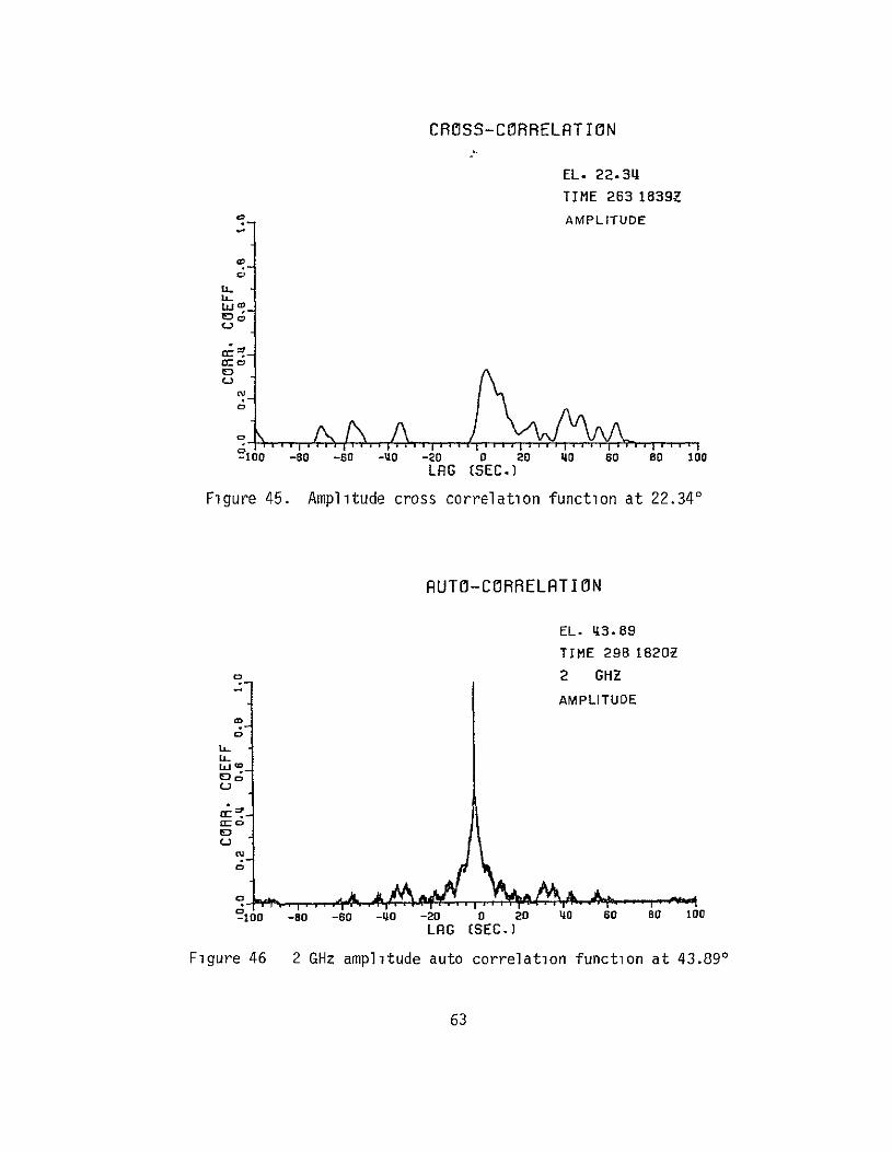
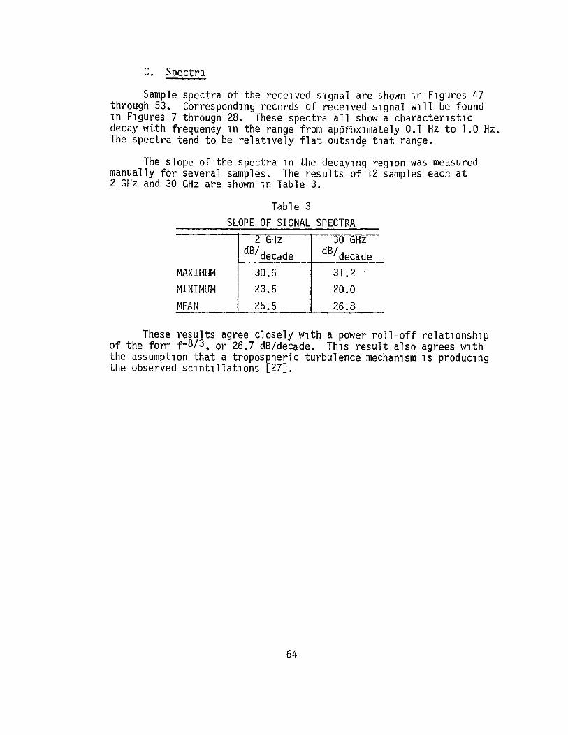
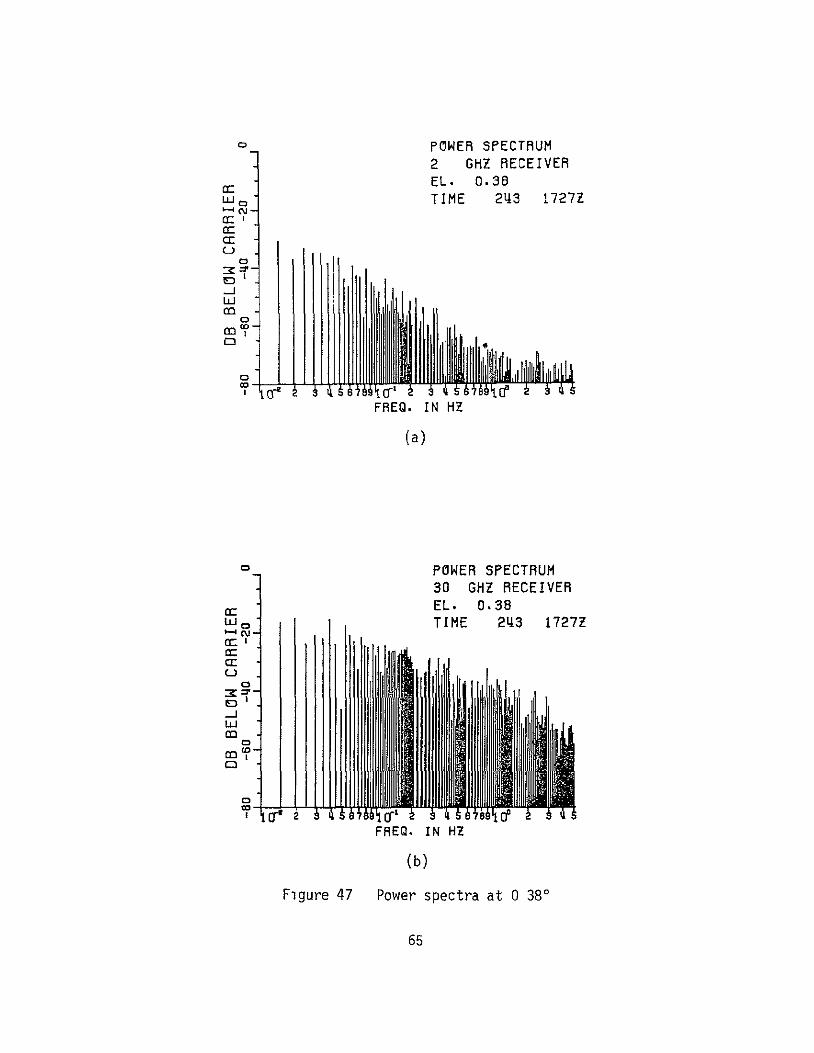
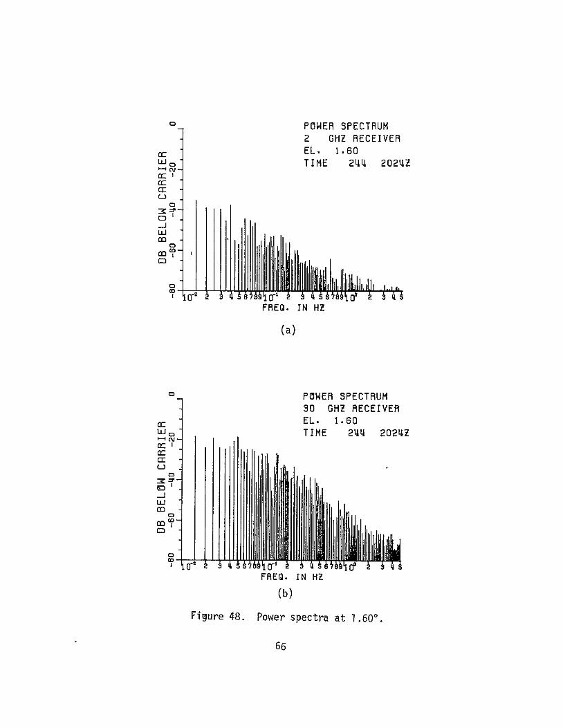
o POWER SPECTRUM
2 GHZ RECEIVER
EL 160 TIME 244 2024Z
=7- N EU
degx
FREQ IN HZ
(a) Cr
U
LI S-Jo o POWER SPECTRUM
~30 GHZ RECEIVER
ccEL 180 wo TIME 244 2024Z
FREQ IN HZ
(b) Figure 48 Power spectra at 1600
66
_ POWER SPECTRUM
2 GHZ RECEIVER
cc L
EL TIME
282 216 2 16Z
-
cc
(a)
U
~POWER SPECTRUM
C IL 30 GHE8RECEIVER
co
UOTIME 246 2 16Z
C
-J
FRE IN HZ
(b)
Figure 49 Power spectra at 2820
67
o POWER SPECTRUM
2 GHZ RECEIVER EL 495
U TIME 247 20292
a
J
LU 0
FREQ IN HZ
(a)
oPOWER SPECTRUM
30 GHZ RECEIVER EL 495
L TIME 247 2029Z
cc - U
a S-
FREQ IN HZ
(b)
Figure 50 Power spectra at 495
68
C POWER SPECTRUM
2 0HZ RECEIVER EL 1811
o TIME 259 1913Z
a 0
m-J
FREQ IN HZ
(a)
o_ POWER SPECTRUM
30 GHZ RECEIVER EL 1811
Uj TIME 259 1913Z
oIm
FREQ IN HZ
(b)
Figure 51 Power spectra at 18 110
69
o POWER SPECTRUM
2 GHZ RECEIVER EL 2234 TIME 263 1842Z
-C
aCr
L)
CD
C
FRED IN HI (a) 0H
oPOWER SPECTRUM
30 GHZ RECEIVER EL 2234 TIME 263 1842Z
-c
m I
FREG IN HZ (b)
Figure 52 Power spectra at 2234
70
b
o POWER SPECTRUM
2 GHZ RECEIVER
EL 4389 TIME 298 1850Z
Cr
C
-J
FREQ IN HZ
Figure 53 Power spectrum at 43890
71
D Fade Distributions
Fade distributions were also studied at several elevation angles averaging about 30000 samples ie 50 minutes each Figures 54 and 55 show the percentage of time a given fade depth was exceeded plotted on a log-normal scale
The curves appear to fit fairly well within each other with increasing elevation However exceptions are clearly seen at 038 and 1600 for both 2 and 30 GHz and at 495 for the 2 GHz signal The reason for the behavior at 495 is not clear at present It should be noted that the 30 GHz fade distribution at this elevation angle does not behave in the same way
The distributions at 2820 are taken to be a representative sample for the higher elevation angle cases and show good fit to straight line approximations indicating that they are Gaussian Even the anomalous distributions show a Gaussian nature over a large portion of their ranges
The fade distributions could in fact be a combination of more than one type of statistic Deviations from the Gaussian curve are prominent for large scintillations Furthermore since the sampling rate is high (10sec) it is possible that the effects of rapid short term scintillations which are believed to be Rayleigh distributed are also being displayed in these distribution curves [28]
Assuming that the dominant long-term statistics at-the higher elevation angles are Gaussian a check was performed at 2820 as follows Let the un-normalized variance be s2 For a log-normal distribution the interval between the 50 and 999 percentile values of the cumulative distribution function - ie 50 and 01 pershycentile values of the fade distribution function - is 31 s[29] For 30 GHz from Figure 55
31 s30 = 86
=27s30
Now from the definition of a2 (Equation (3-6)) we can write that
0 ogloG2 =
dB K1
2zdB
= K110os
72
9999 FADE DISTRIBUTIONS
2 GHz 999 998 -
99 gtt
AA A
ELEVATION (DEG)
98 bull A 0
X 038 160
95 9-0D A o628228 04 A 495
90 x 0 1811 + 1+ 4381
x c0 o X
w 70 x w + E3
x 60shy
lt 50 + 40- 13
350- 0 0
C20 + x
1-0- A3 X x~
ox x 5-+ C X
+ A x X XX
2 I-
+ A
05 a
02- 0
0I 005
001 0 1 5 4 5 6 7 a 9
FADE (d8)
Figure 54 Fade distributions at 2 GHz
73
9999
999
998 -
FADE DISTRIBUTIONS
30 GHz
w w o x
99
98
95
80
A
X
x
ELEVATION (DEG)
038 x 160 0 282 A 495
1811 + 4381
600
650 a
S40 -x
w30-
-20 20
A
A x 0
10-0+D
0+ 0 5-
2--x 5
A30
Abull 0
X
0
S
X X
X OX x
2- A X
02- I A- 0 0 x
021
0010 5 10 15 20 25 30 35 40 45
FADE (d8)
Figure 55 Fade distributions at 30 GHz
74
From Figure 27 average log amplitude variance at 282
2 a ZdB 30 = - 115 dB
-115
s30 = (20 loglo e) 1 010
s30 = 234
This compares favorably with s as calculated from Figure 55
Similarly for 2 GHz at 282 from Figure 54
31 s2 = 23
= 074s2
from Figure 27 and following the same procedure as above
s2 = 045
The discrepancies could be partly due to the fact that the values shown in Figure 27 are calculated for 205 second intervals only and then averaged over each elevation angle These are therefore shortshyterm statistics and would tend to be Rayleigh distributed whereas the distributions in Figures 54 and 55 were calculated over the whole elevation angle directly these tend to be Gaussian Further the deviations from the log-normal curve for strong scintillations would also affect the result
75
CHAPTER V CONCLUSIONS
The results of the experiment are summarized in this chapter
A The Received Signals
The received siqnals show several types of fluctuations
a) Very low elevation angles (less than 40)
(i) Slow rises and fades of tens of dB over periods of tens of minutes
(ii) Faster fluctuations or scintillations with durations of a few minutes or less occurring continuously
(il) Continuous rapid scintillations of a dB or less
(iv) Slow roller-type fading is also seen However the high signal correlation found rules out ground reflection effects (Appendix D)
b) Low elevation angles (40 to 100)
(1) Very slow changes in mean level of a few dB over 30 minutes or more
(ii) Faster scintillations of several dB with periods of a few tens of seconds
(il) Continuous rapid scintillations
c) Medium elevation angles (10 - 44)
(1) Virtually no change in mean level except during precipitation events
(ii) Enhanced scintillations of a few dB for a few minutes are now visible
(iii) Continuous rapid scintillations
Scintillations were observed at all times in clear air and also in the presence of non-precipitating clouds At the highest elevation angles there appears to be a tendency for the scintillations to be enhanced in the presence of non-precipitating cumulus clouds
76
In the following discussion the symbols A and k are used to denote amplitude and log amplitude quantities respectively The symbol V is used to denote either one in general
B Variances
Amplitude and log variances are defined in Equations (3-4) and(3-6)
The range of the variances at any elevation angle exceeded 20 dB at times However the average variances followed a cosecant power law with elevation angle fairly well
Table 4
2 A [CSC(EL)] B
2 GHz 30 GHz
A B A B
10-4 9 12 162 10-4 3 214A 2 plusmn3
-43 a 2 10-49 162 10 220plusmn2 plusmn3
The fairly large error bounds have been introduced to account for the limited data Observations over extended periods under widely varying weather conditions would give a closer estimate The exponents B compare well in their range of error with the theoretical value B = 1833 for Kolmogorov type turbulence
As a refinement a spherical earth model was assumed with a uniform homogeneous atmosphere of effective height h km When this was fitted to the data the results were as follows
77
Table 5
a2 -A LB
L =Ih2 + 2hR + R2 Sin2e - RSine
R = 8479 km 0 = elevation anole
2 GHz 30 GHz
A B hkm A B hkm
10- 6 5 10- 6 4A 187 62 248 61plusmn2 plusmn1 plusmn3 plusmnI
2 10-6 4 187 61 1061 249 45
plusmn2 plusmnIt3
A reduction inmean square error of between 5 to 15 is obtained However in general the much simpler cosecant law
a A [CSC(amp)]B
appears to be quite adequate for elevation angles above 40
The 30 GHz data obtained during the departure of ATS-6 in 1975
agree well with the present data
The ratio of variances a2 1 2 has a mean value of 92 dB
A value of 44 dB was obtained for a2A30l 2A inthe 1975 measureshyments 3
C Received Signal Levels
The relative received signal levels show a strong dependence on elevation angle for elevations less than 5 They are relatively independent of elevation thereafter The drop in signal levels at low elevation angles are much greater than simple path-loss calcushylations predict
78
D Cross Correlations
Cross correlation was evaluated as a function of elevation angle Both the amplitude and log amplitude cross correlations are identical for elevations above 5 Below this angle they diverge slightly The cross correlations appear to follow a cosecant law with an exponent of 161 to 166
The average amplitude correlation was found to agree well with that predicted by Lee and Harp for the frequency ratio of 1446 The 1975 data also show good agreement with the predicted value for a frequency ratio of 15
Representative samples of auto and cross correlation functions with time lag were also shown Cross correlation lag ranged from 0 to about 10 seconds with most of the values in the region of 0 to 5 seconds Significant correlation was not found for lags exceeding 15 seconds
E Power Spectra
The power spectra of the 2 and 30 GHz signals show a characshyteristic decay with freguncy in the region of 01 to 1 Hz The roll-off follows the f- law agreeing with the assumption of tropospheric turbulence as a dominant mechanism in the samples analyzed
F Fade Distributions
Fade distributions were calculated for selected elevation angles The results suggest dominant Gaussian distributions However there is significant deviation from the normal curve for strong scintillations at low elevation angles
Fades in excess of 30 dB at 30 GHz and 7 dB at 2 GHz were observed for 5 of the time at low elevation angles These dropped to 1 dB and 06 dB respectively at 410
G Summary
Microwave signal amplitude scintillation characteristics were studied on earth-space paths for elevation angles varying from 04 to 439 using the ATS-6 satellite Beacon signals at two frequencies 2 GHz and 30 GHz were monitored simultaneously The results are consistent with similar measurements made earlier at 20 and 30 GHz
Variances are modeled well by the cosecant law and by a homoshygeneous spherical earth model with an equivalent height of 6 km Agreement with the Kolmogorov turbulence model is found The mean ratio of the variances is 94 dB
79
The correlation between the two signals was as high as 04 at low elevation angles and follows a cosecant law The average value is close to that predicted by Lee and Harp for the ratio of these frequencies Correlation lags were in the 0 - 5 second range and significant correlation was not found for lags exCeeding 15 seconds The lags may be attributed to wind fields as modeled by Lee and Harp
The power spectra at both 2 and 30 GHz show an f-8 3 roll-off in the 01 to 1 Hz range This agrees with the assumption of tropospheric turbulence as the dominant mechanism
Mean signal levels dropped sharply below predicted values at elevation angles below about 40 Fades exceeded 30 dB and 7 dB at 30 and 2 GHz respectively for 5 of the time at low elevation angles These reduced to less than I dB at an elevation of 410
The long term statistics are Gaussian except for strong scintillations when significant divergence from the Gaussian distribution was found
80
APPENDIX A EDITED TAPE FORMAT
The format of the final edited working digital magnetic tape corrected for receiver calibration characteristics is shown
Packed Tape 48 File Format
File No Day No of Records (1976)
1 243 244 38 2 245 40 3 246 247 100 4 251 254 255 47 5 257 - 263 265 266 165 6 271 18 7 275 277 281 54 8 291 292 294 296 298 70
Packed Tape 48 Record Format
Record Length = 2555 Integer words
words 1-10 = Header Wl = No of words in Record W2 = Day W3 = Hour W4 = Minute W5 = Second W6 = millisecond W7 = Azimuth (milli degrees) W8 = Elevation (milli degrees) W9 = Record Type (10 a 110 sec rate samples) W1O = Data Status
Bit = -Bit 1 = 2 GHz Rec Bit 2 = 30 GHz Rec
If receiver is on and data is usable the
corresponding bit = 1
Words 11 - 2555
Wll - W2058 max = Packed data words
in 01 dB Bits 0 - 11 2 GHz below reference IBits 12 -23 30 GHz
Remaining words are unused
81
APPENDIX B TABLE OF USEFUL DATA PERIODS
The data recorded during the experiment were edited by eliminating periods of equipment adjustment antenna peaking or adjustment and data corrupted by ground reflections at elevation angles below 038
B-I This section of the Appendix shows the periods duringwhich the data was considered usable after editing
a) Column 1
Entry number
b) Column 234
Time of day (Days Hours Minutes) Greenwich Mean Time
c) Column 56
Nominal Azimuth and Elevation angles in degrees
d) Column 78
These give the external additional attenuators in the receiver which were not directlyrecorded by the data recording system
e) Column 9
The status of the data is given in this column as an octal number as shown below
Bit no 2 1 0
Status I
Receiver 30 GHz 2 GHz 360 MHz
An acceptable data period is indicated by the corresponding bit being set to 1
82
NO OAY HOUR MIN A1 M ELEV 30 GHZ e GHZ STAT (nul (DEG) (DB) (DIR)
1 e6 10 0710l - A 14
e43 4 0 97I0 -4c4 1 1 6 37 24 -474f 6P 6 6
4 4 1 97 4F 3 o b 1b 24o4a 974F 6p 0 4 6 446 1J )2 9746 6p 1 0 7 246 19 18 97b7 45 0 6 4
8 )
a43 3L
3 it)
9763 97ol
47
47 C 0
8 b
7 r
10 2115 2L 17 9761 47 0 7
11 e45lfl -A 97b3 47 1 1 0 oe e44 bU 9eQ19 4 e 7
16 244 6 0 9819 74 0 n 5 14 244 9 50 9860 99 L 0 5
U0lb lamp
-244
i ) 1n
a 9
9AO 9830
99
99 3 b
0 1
1 4
j7 241 10 A6 9aoO 97 5 04 la 244 1ii 57 q81 5 1 1008 10 0 5
39 244 1x 30 9837 135 le 14 20 e44 IB 50 9850 154 10 3 4
244 0 I 98D9 lobO I0 2 6
22 44 41 0 959 lbO lu 2 I 26 24
45 445
1 2
54 8
9895 9P95
17017o 1030 22 27 2b e-45 6 1 9 g 95FT L7nIC 2 5
NO UAY HOUR MIN AZi M ELLV 60 GFl7 wbi$Z STAT (fLG) (DEG) (UP) (U )
4b 4 56 9913 181 1L 2 4 eL45 U 85 9913 161 0 2 5 e45 7 30 9p2 196 10 2 5
29 e45 9 20 99e2 196 10 2 4 3U =45 9 4u 99e7 211 ILI 2 5 31 11 4b50 90e7 211 16 2 U 52 24b 12 O 9941 21 3 I 5 36 245 13 15 9931 P63 i( 2 4 -4 c45
45 It 14
0 3Q
9961 99 54
263 247
IG IC
2
4 4
o6 d45 16 30 3 9 22b7 10 2 4 37 245 lb M1 9q47 b6 IC 2 4 38 245 z 6 9b6 271 10 2 6 35 40
45 e46
21 1
U 54
9b6 9994
71 26p
IC 10
2 2
0 7
41 246 0 9994 282 10 2 5 12 e46 4 U 100116 p6C 10 2 5 41 246 5 6 10006 28q 10 2 7 L4 246 b U 30f06 289 10 2 fl I b 6 17 4 10040 72 10 2 6 46 246 IS 4 10040 37 10 4 u7 246 19 U 3Lin Q $7 1 2 4 48 246 2C 4 10054 --82 I0 2 6
ee46 21 U 1On54 Ab2 10 2 4 50 a46 21 30 lO0Dt 6b2 10 2 0
NO UAY HOUR IIN AZI fuI ELEV 60 GIZ 2 bHZ STAT (DEG) (PLG) (DP) (Or)
51 47 b 9 10136 474 22 2 6 52 247 16 10153 474 22 2 4 So d47 17 U 30133 483 22 2 4 594 247 je 54 10147 491 22 2 5 95 e4 7 0 19 101 bE 495 22 2 7 5( 247 21 2 101b59 495 22 2 0 57 248 16 55 10268 594 22 2 5 58 248 19 U 10247 602 22 2 0 59 251 j7 4 10545 92c) 1) 7 60 ebl 17 2U 10545 929 2 0 0 61 e54 11 6 10850 1222 22 0 7 62 254 12 95 1P50 12e2 22 6 66 e 32 n UPSbU 1222 amp2 0 7 64 254 12 30 XOU50 1222 2 0 0 65 e55 15 34 10a67 16b3 22 0 7 66 255 16 25 10q67 163 22 0 0 67 e57 23 5 ltf 156 22 0 7 f6 eb7 14 U 111L 1t65 22 0 o 69 258 36 11316 17o4 22 0 6
r70 258 19 50 11316 1704 22 0 0 71 259 18 31 l11o2 1811 22 0 72 259 19 30 31462 1811 2a 0 0 76 260 19 29 11550 1918 22 0 6 74 260 19 26 11551 1918 22 0 4 7t 260 19 27 11550 1918 22 2 6
N10 DAY HOUR MIN AziM1 ELEV O GH2 2 6H7 STAT ( Lu ( Lu) (OH) (UU)
76 260 19 51 11 0 19018 22 2 0 77 261 i6 31 1r453 1998 22 7b e61 IN 31 111453 1998 2 2 u 79 262 2 118G3 r216 22 2 E bu 61 20 59 l1v 263 0 Pl 266 1A 19 1117 2264 22 2E 82 263 19 40 llq17 2234 1 2
86 e65 49 12a V 2416 P2 2 6
84 265 14 30 12158 2416 2 2 0 pound5 2E6 i1 1 122~v a 3t4 dc -
86 e7
266 266
16 -14
37 1
1228Q 12LP39
2r14 5o1
22 2
2 U
86 266 14 30 1226 2514 e2 0 8 271 4 52 12922 2923 22 0 6 9 e7 Q 1 2 94e 2SZ3 22 0 0 91 e71 4 66 1C942 2c3 22 6 92 eTi 5 51 1292 2926 22 2 0 96 e5 17 06 166i0 33br 22 2 6 94 475 18 50 ii0 53b 22 2 0 95 e77 2U 52 13972 653 2 2 96 277 21 56 15972 3566 22 P 0 q7 281 1 )I 144kj ULu2 22 2 6 9 t 281 1 41 14641 5 02 2e 2 0 99 291 2U b 14764 4aiq 22 2 6
IOU eql 21 0 167a 4119 22 2 U
NO t AY HOUR MIN AZIN ELEV 30 GHZ 2 GHZ STAT (uEb) (WEG) (08) (JB)
101 e92 l 5 169 16 44 22 6 102 292 19 15 16076 43Q44 22 2 0 106 94 C 55 17278 63A 22 b 14 2994 6 30 1727P 413A 22 2 0
105 296 134 27n414 4381 2 C 1o6 96 15 0 1784 4361 22 2 0 In d98 1e 20 18342 4389 22 2 6 lob 98 19 0 18342 43a9 22 2 0
B-2 The durations of the data periods used in the calculations in this report are given below
Elevation (degrees)
038 048 074 160 170 271 282 289 372 382 474 495
929 1222 1363 1565
Duration (minutes)
32 19 20 46 71 57 61 57 60 56 52 42
16 84 54 57
Elevation (degrees)
1704 1811 1918 1998 2135 2234 2416 2514 2923 3365 3536 3802
4319 4344 4358 4381 4389
Duration (minutes)
54 59 81 59 57 71 41 50 57 57 57 56
52 57 35 66 40
OF POOR QUPLrfORIG19M FAOt 1S
88
APPENDIX C COMMENTS ON LOG AND AMPLITUDE VARIANCE
Expanding the definition of log variance (Equation (3-6))
N 12NN2 1 1a = iL-- I~N 1 kJ KIN i=1( l 22
2 1 N a
= (120 log101 0a 20 lOgio (C-1)
K2N 11 a0 NJ 2 1091 ) 10
but
a a lglO a9 l - + lg0 ashy
0 a o
N a2 202 N O - 1 1oq 0 -- + loK10 To - logl - +10
K1IN i=1(I a o yl
a09lt2N aya
KaN1 20 10
20 Y2 1
1090 logoeK =a I a
Kl = lOg0 e loge
a a
2 a N
a_Y (20 loglo -_1I N I loge l 2 2 (20 logloe)2
(20 logloe) I a j=1 a
89
For small scintillations a
a 1
lo e = - Jrl
Also
2 1 Cf
ala
(a 1 1
a) (C-2)
2= N a
ao
2 N (a shy T)2
2 - 02(-3)
2 a2 for small scintillations
The computed results show excellent agreement even at low elevation angles (ie large scintillations)
Further Fried has shown [30] from energy considerations that
a2p _-T (C-4)
(This result has been adapted to be consistent with the definitions used in this study)
90
0
Now Z shows a sharp drop at low elevat~o9 angles It seen n Figure 56 where the numerical values of K1 a z(NB not pounddB
are plotted that this behavior is in fact reflected
The observations are therefore consistent However the reason for the sharp knee in the mean levels is yet to be determined
LOG-VRRIRNCE
+ 2 GHz
x 30 GHz
x2 IX)2
ci X X
CD
x
+
5 10 15 20 25 30 35 40 45 ELEV (DEG)
Figure 56 Log amplitude variance (numeric)
91
APPENDIX D RECEIVED SIGNALS AT LOW ELEVATION ANGLES
AND MULTIPATH EFFECTS
The mechanism which causes the amplitude scintillations may be regarded as being either refractive or multipath in nature Low two-frequency correlation would be expected if multipath were the dominant factor because an arbitrary differential path length cannot produce simultaneous subtractive or additive phasing at the two wavelengths employed as shown below [17]
Subtractive multipath phasing will occur at a wavelength of X1 if the difference between the two path lengths satisfy
AL = (2n+l) -7 n = O 2
Similarly at a second wavelength X2
AL = (2m+l) 2p m = 0 1 2
Therefore
(2n+l)A 1 = (2m+l)A 2
But in general
A I = PA2 where P is an arbitrary number
So that
P(2n+l) = 2m+l (D-1)
For example the 1975 measurements were performed simultaneously at 20 and 30 GHz therefore P = 32 Then
3 (2n+l) = 2m+l
or 3(2n+l) = 2(2m+l) (D-2)
However the left side of Equation (D-2) is odd and the right side is even Therefore simultaneous fading due to simple multishypath propagation cannot occur This result contradicts the very high correlations observed between the 20 and 30 GHz signal fluctuations Thus one is forced to conclude that the observed fluctuations are not a result of a simple multipath mechanism
92
APPENDIX E SUMMARY OF DEFINITIONS
a(t) is a positive real signal amplitude a are discrete samples of a(t) at equal intervals over a time interval T a(t) has been corrected for receiver nonlinearities The relative amplitudeis defined to be
a A =- I I a0
and the relative log amplitude as
20 logO ashy=
where a0 is an arbitrary constant
93
AMPLITUDE LOG AMPLITUDE RELATIONSHIP FORSMALL SCINTILLATIONS
= _ A(t) dt = fT1 (t) dt
MEAN JT d z J T N t T 20 loglo
1= 1 L1=1
MEAN TOTAL POWER I JA2(t) t (MEAN SQUARE) N 2 A vdBz
N i1I
VARIANCE ~ (NORMALIZED TO DC POWER)
2 AT
1jf A(t+i2 A N
dt 2 1 T
Wtd NaAC
2-22
NA 1 1 KNK~I 1lN1=
AMPLITUDE LOG AMPLITUDE
CORRELATION
COEFFICIENT
12 --I (Am (t)-l)(A2 (t+T)-T 2 )dt
PA(t)T Al- O 0A1 A1I[2
(A 2- A-I2 I (A (A2 A2 )
1N=l2 0= A1 A2
2 1 z(t)-T( t+r)-12 )dt
f 2K1l 2
1I2
N ( lI- -I)( 21+j- 2) 1 )
K1N 1=] lP2
RELATIONSHIP FOR SMALL SCINTILLATIONS
PA12 v 2
K 20 logloe T = j T IT
REFERENCES
[1] L Cuccia W Quan and C Hellman Above 10 GHz Satcom Bands Spur New Earth Terminal Development Microwave System News March 1977 p 3738
[2] L Cuccia et al Op Cit p 46-50
[3] D E Kerr Propagation of Short Radio Waves McGraw Hill 1964
[4] B R Bean and E J Dutton Radio Meteorology Dover 1968
[5] D C Livingston The Physics of Microwave Propagation Prentice Hall 1970
[6] Propagation Factors in Space Communications AGARD Conference Proceedings No 3 W J Mackay and Co 1967
[7] P David and J Voge Propagation of Radio Waves Pergamon Press 1969
[8] Communications Satellite Corporation COMSAT Technical Review Vol 3 No 1 to Vol 5 No 2
[9] E V Appleton URSI Proceedings Washington 1927
[10] E H Whitney and S Basu The Effect of lonosphereic Scintillation on VHFUHF satellite Communications Radio Science Vol 12 No 1 1977 p 123-133
[11] Aarons et al Radio Astronomy Measurements at VHF and Microwaves Proceedings IRE January 1958 p 325-333
[12] L A Hoffman et al Propagation Observations at 32 Millishymeters Proceedings IEEE Vol 54 No 4 April 1966
[13] L J Ippolito Effects of Precipitation on 153 and 3165 GHz Earth-Space Transmission With the ATS-V Satellite Proceedings IEEE Vol 59 No 2 1971
[14] L J Ippolito ATS-6 Millimeter WaVe Propaqation and Communishycations Experiments at 20 and 30 GHz IEEE Transactions Vol AES-ll No 6 1975
[15] Goddard Space Flight Center ATS-F and -G Data Book September 1972 p A39-A42
96
[16] D B Hodge and D M Theobold Scintillations Observed on the ATS-6 20 and 30 GHz Downlinks URSIUSNC meeting Boulder Colorado October 1975
[17] D B Hodge D M Theobold and R C Taylor ATS-6 Millimeter Wavelength Propagation Experiment Report 3863-6 January 1976 The Ohio State University ElectroScience Laboratory Department of Electrical Engineerng prepared under Contract NAS5-21983 For NASA Goddard
[18] V I Tatarski Wave Propagation in a Turbulent Medium Israel Program for Scientific Translation Jerusalem 1971
[19] R F F11ipowski and E I Muehldorf Space Communication Systems Prentice Hall 1965
[20] G N Krassner Introduction to Space Communication Systems Chapter 4 McGraw Hill 1964
[21] D M Theobold and D B Hodge ATS-6 Millimeter Wavelength Propagation Experiment Report 3863-4 April 1975 The Ohio State University ElectroScience Laboratory Department of Electrical Engineering prepared under Contract NAS5-21983 for NASA Goddard
[22] B H Briggs and I A Parkin On The Variation of Radio Star and Satellite Scintillations with Zenith Angle J Atmos Terr Phys 25 p 339-366
[23] A Kolmogorov Turbulence Classic Papers on Statistical Theory S K Friedlander and L Topper Eds New York Interscience 1961 p 151
[24] A Benoit Signal Attenuation Due to Neutral Oxygen and Water Vapor Rain and Clouds The Microwave Journal November 1968 p 73-80
[25] K S McCormick and L A Maynard Measurements of SHF Tropospheric Fading Along Earth-Space Paths at Low Elevation Angles Electronics Letters Vol 8 1972 p 274
[26] R W Lee and J C Harp Weak Scattering in Random Media with Applications to Remote Probing Proc IEEE Vol 57 1969 p 375-406
[27] R S Lawrence and J W Strohbehn ASurvey of Clear Air Propagation Effects Relevent to Optical Communications Proc IEEE Vol 58 No 10 October 1970 pp 15371538
97
[28] P F Panter Com unication Systems Design McGraw Hill 1972
pp 347-358
[29] P F Panter Op Cit p 355
[30] D L Fried Optical Resolution Through a Randomly Inhomoshygeneous Medium for Very Long and Very Short Exposures J Opt Soc Am 56 October 1966 pp 1372-1379
98
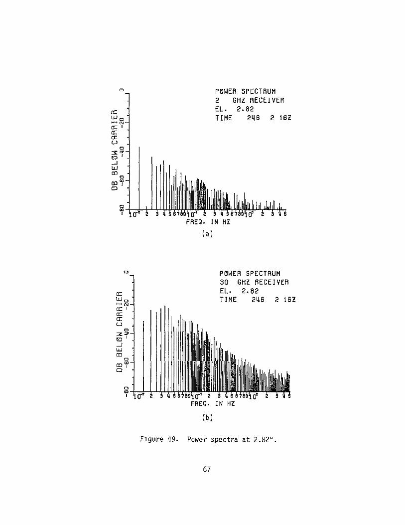
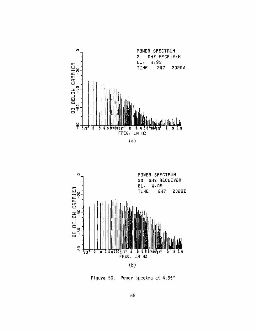
o POWER SPECTRUM
2 GHZ RECEIVER EL 495
U TIME 247 20292
a
J
LU 0
FREQ IN HZ
(a)
oPOWER SPECTRUM
30 GHZ RECEIVER EL 495
L TIME 247 2029Z
cc - U
a S-
FREQ IN HZ
(b)
Figure 50 Power spectra at 495
68
C POWER SPECTRUM
2 0HZ RECEIVER EL 1811
o TIME 259 1913Z
a 0
m-J
FREQ IN HZ
(a)
o_ POWER SPECTRUM
30 GHZ RECEIVER EL 1811
Uj TIME 259 1913Z
oIm
FREQ IN HZ
(b)
Figure 51 Power spectra at 18 110
69
o POWER SPECTRUM
2 GHZ RECEIVER EL 2234 TIME 263 1842Z
-C
aCr
L)
CD
C
FRED IN HI (a) 0H
oPOWER SPECTRUM
30 GHZ RECEIVER EL 2234 TIME 263 1842Z
-c
m I
FREG IN HZ (b)
Figure 52 Power spectra at 2234
70
b
o POWER SPECTRUM
2 GHZ RECEIVER
EL 4389 TIME 298 1850Z
Cr
C
-J
FREQ IN HZ
Figure 53 Power spectrum at 43890
71
D Fade Distributions
Fade distributions were also studied at several elevation angles averaging about 30000 samples ie 50 minutes each Figures 54 and 55 show the percentage of time a given fade depth was exceeded plotted on a log-normal scale
The curves appear to fit fairly well within each other with increasing elevation However exceptions are clearly seen at 038 and 1600 for both 2 and 30 GHz and at 495 for the 2 GHz signal The reason for the behavior at 495 is not clear at present It should be noted that the 30 GHz fade distribution at this elevation angle does not behave in the same way
The distributions at 2820 are taken to be a representative sample for the higher elevation angle cases and show good fit to straight line approximations indicating that they are Gaussian Even the anomalous distributions show a Gaussian nature over a large portion of their ranges
The fade distributions could in fact be a combination of more than one type of statistic Deviations from the Gaussian curve are prominent for large scintillations Furthermore since the sampling rate is high (10sec) it is possible that the effects of rapid short term scintillations which are believed to be Rayleigh distributed are also being displayed in these distribution curves [28]
Assuming that the dominant long-term statistics at-the higher elevation angles are Gaussian a check was performed at 2820 as follows Let the un-normalized variance be s2 For a log-normal distribution the interval between the 50 and 999 percentile values of the cumulative distribution function - ie 50 and 01 pershycentile values of the fade distribution function - is 31 s[29] For 30 GHz from Figure 55
31 s30 = 86
=27s30
Now from the definition of a2 (Equation (3-6)) we can write that
0 ogloG2 =
dB K1
2zdB
= K110os
72
9999 FADE DISTRIBUTIONS
2 GHz 999 998 -
99 gtt
AA A
ELEVATION (DEG)
98 bull A 0
X 038 160
95 9-0D A o628228 04 A 495
90 x 0 1811 + 1+ 4381
x c0 o X
w 70 x w + E3
x 60shy
lt 50 + 40- 13
350- 0 0
C20 + x
1-0- A3 X x~
ox x 5-+ C X
+ A x X XX
2 I-
+ A
05 a
02- 0
0I 005
001 0 1 5 4 5 6 7 a 9
FADE (d8)
Figure 54 Fade distributions at 2 GHz
73
9999
999
998 -
FADE DISTRIBUTIONS
30 GHz
w w o x
99
98
95
80
A
X
x
ELEVATION (DEG)
038 x 160 0 282 A 495
1811 + 4381
600
650 a
S40 -x
w30-
-20 20
A
A x 0
10-0+D
0+ 0 5-
2--x 5
A30
Abull 0
X
0
S
X X
X OX x
2- A X
02- I A- 0 0 x
021
0010 5 10 15 20 25 30 35 40 45
FADE (d8)
Figure 55 Fade distributions at 30 GHz
74
From Figure 27 average log amplitude variance at 282
2 a ZdB 30 = - 115 dB
-115
s30 = (20 loglo e) 1 010
s30 = 234
This compares favorably with s as calculated from Figure 55
Similarly for 2 GHz at 282 from Figure 54
31 s2 = 23
= 074s2
from Figure 27 and following the same procedure as above
s2 = 045
The discrepancies could be partly due to the fact that the values shown in Figure 27 are calculated for 205 second intervals only and then averaged over each elevation angle These are therefore shortshyterm statistics and would tend to be Rayleigh distributed whereas the distributions in Figures 54 and 55 were calculated over the whole elevation angle directly these tend to be Gaussian Further the deviations from the log-normal curve for strong scintillations would also affect the result
75
CHAPTER V CONCLUSIONS
The results of the experiment are summarized in this chapter
A The Received Signals
The received siqnals show several types of fluctuations
a) Very low elevation angles (less than 40)
(i) Slow rises and fades of tens of dB over periods of tens of minutes
(ii) Faster fluctuations or scintillations with durations of a few minutes or less occurring continuously
(il) Continuous rapid scintillations of a dB or less
(iv) Slow roller-type fading is also seen However the high signal correlation found rules out ground reflection effects (Appendix D)
b) Low elevation angles (40 to 100)
(1) Very slow changes in mean level of a few dB over 30 minutes or more
(ii) Faster scintillations of several dB with periods of a few tens of seconds
(il) Continuous rapid scintillations
c) Medium elevation angles (10 - 44)
(1) Virtually no change in mean level except during precipitation events
(ii) Enhanced scintillations of a few dB for a few minutes are now visible
(iii) Continuous rapid scintillations
Scintillations were observed at all times in clear air and also in the presence of non-precipitating clouds At the highest elevation angles there appears to be a tendency for the scintillations to be enhanced in the presence of non-precipitating cumulus clouds
76
In the following discussion the symbols A and k are used to denote amplitude and log amplitude quantities respectively The symbol V is used to denote either one in general
B Variances
Amplitude and log variances are defined in Equations (3-4) and(3-6)
The range of the variances at any elevation angle exceeded 20 dB at times However the average variances followed a cosecant power law with elevation angle fairly well
Table 4
2 A [CSC(EL)] B
2 GHz 30 GHz
A B A B
10-4 9 12 162 10-4 3 214A 2 plusmn3
-43 a 2 10-49 162 10 220plusmn2 plusmn3
The fairly large error bounds have been introduced to account for the limited data Observations over extended periods under widely varying weather conditions would give a closer estimate The exponents B compare well in their range of error with the theoretical value B = 1833 for Kolmogorov type turbulence
As a refinement a spherical earth model was assumed with a uniform homogeneous atmosphere of effective height h km When this was fitted to the data the results were as follows
77
Table 5
a2 -A LB
L =Ih2 + 2hR + R2 Sin2e - RSine
R = 8479 km 0 = elevation anole
2 GHz 30 GHz
A B hkm A B hkm
10- 6 5 10- 6 4A 187 62 248 61plusmn2 plusmn1 plusmn3 plusmnI
2 10-6 4 187 61 1061 249 45
plusmn2 plusmnIt3
A reduction inmean square error of between 5 to 15 is obtained However in general the much simpler cosecant law
a A [CSC(amp)]B
appears to be quite adequate for elevation angles above 40
The 30 GHz data obtained during the departure of ATS-6 in 1975
agree well with the present data
The ratio of variances a2 1 2 has a mean value of 92 dB
A value of 44 dB was obtained for a2A30l 2A inthe 1975 measureshyments 3
C Received Signal Levels
The relative received signal levels show a strong dependence on elevation angle for elevations less than 5 They are relatively independent of elevation thereafter The drop in signal levels at low elevation angles are much greater than simple path-loss calcushylations predict
78
D Cross Correlations
Cross correlation was evaluated as a function of elevation angle Both the amplitude and log amplitude cross correlations are identical for elevations above 5 Below this angle they diverge slightly The cross correlations appear to follow a cosecant law with an exponent of 161 to 166
The average amplitude correlation was found to agree well with that predicted by Lee and Harp for the frequency ratio of 1446 The 1975 data also show good agreement with the predicted value for a frequency ratio of 15
Representative samples of auto and cross correlation functions with time lag were also shown Cross correlation lag ranged from 0 to about 10 seconds with most of the values in the region of 0 to 5 seconds Significant correlation was not found for lags exceeding 15 seconds
E Power Spectra
The power spectra of the 2 and 30 GHz signals show a characshyteristic decay with freguncy in the region of 01 to 1 Hz The roll-off follows the f- law agreeing with the assumption of tropospheric turbulence as a dominant mechanism in the samples analyzed
F Fade Distributions
Fade distributions were calculated for selected elevation angles The results suggest dominant Gaussian distributions However there is significant deviation from the normal curve for strong scintillations at low elevation angles
Fades in excess of 30 dB at 30 GHz and 7 dB at 2 GHz were observed for 5 of the time at low elevation angles These dropped to 1 dB and 06 dB respectively at 410
G Summary
Microwave signal amplitude scintillation characteristics were studied on earth-space paths for elevation angles varying from 04 to 439 using the ATS-6 satellite Beacon signals at two frequencies 2 GHz and 30 GHz were monitored simultaneously The results are consistent with similar measurements made earlier at 20 and 30 GHz
Variances are modeled well by the cosecant law and by a homoshygeneous spherical earth model with an equivalent height of 6 km Agreement with the Kolmogorov turbulence model is found The mean ratio of the variances is 94 dB
79
The correlation between the two signals was as high as 04 at low elevation angles and follows a cosecant law The average value is close to that predicted by Lee and Harp for the ratio of these frequencies Correlation lags were in the 0 - 5 second range and significant correlation was not found for lags exCeeding 15 seconds The lags may be attributed to wind fields as modeled by Lee and Harp
The power spectra at both 2 and 30 GHz show an f-8 3 roll-off in the 01 to 1 Hz range This agrees with the assumption of tropospheric turbulence as the dominant mechanism
Mean signal levels dropped sharply below predicted values at elevation angles below about 40 Fades exceeded 30 dB and 7 dB at 30 and 2 GHz respectively for 5 of the time at low elevation angles These reduced to less than I dB at an elevation of 410
The long term statistics are Gaussian except for strong scintillations when significant divergence from the Gaussian distribution was found
80
APPENDIX A EDITED TAPE FORMAT
The format of the final edited working digital magnetic tape corrected for receiver calibration characteristics is shown
Packed Tape 48 File Format
File No Day No of Records (1976)
1 243 244 38 2 245 40 3 246 247 100 4 251 254 255 47 5 257 - 263 265 266 165 6 271 18 7 275 277 281 54 8 291 292 294 296 298 70
Packed Tape 48 Record Format
Record Length = 2555 Integer words
words 1-10 = Header Wl = No of words in Record W2 = Day W3 = Hour W4 = Minute W5 = Second W6 = millisecond W7 = Azimuth (milli degrees) W8 = Elevation (milli degrees) W9 = Record Type (10 a 110 sec rate samples) W1O = Data Status
Bit = -Bit 1 = 2 GHz Rec Bit 2 = 30 GHz Rec
If receiver is on and data is usable the
corresponding bit = 1
Words 11 - 2555
Wll - W2058 max = Packed data words
in 01 dB Bits 0 - 11 2 GHz below reference IBits 12 -23 30 GHz
Remaining words are unused
81
APPENDIX B TABLE OF USEFUL DATA PERIODS
The data recorded during the experiment were edited by eliminating periods of equipment adjustment antenna peaking or adjustment and data corrupted by ground reflections at elevation angles below 038
B-I This section of the Appendix shows the periods duringwhich the data was considered usable after editing
a) Column 1
Entry number
b) Column 234
Time of day (Days Hours Minutes) Greenwich Mean Time
c) Column 56
Nominal Azimuth and Elevation angles in degrees
d) Column 78
These give the external additional attenuators in the receiver which were not directlyrecorded by the data recording system
e) Column 9
The status of the data is given in this column as an octal number as shown below
Bit no 2 1 0
Status I
Receiver 30 GHz 2 GHz 360 MHz
An acceptable data period is indicated by the corresponding bit being set to 1
82
NO OAY HOUR MIN A1 M ELEV 30 GHZ e GHZ STAT (nul (DEG) (DB) (DIR)
1 e6 10 0710l - A 14
e43 4 0 97I0 -4c4 1 1 6 37 24 -474f 6P 6 6
4 4 1 97 4F 3 o b 1b 24o4a 974F 6p 0 4 6 446 1J )2 9746 6p 1 0 7 246 19 18 97b7 45 0 6 4
8 )
a43 3L
3 it)
9763 97ol
47
47 C 0
8 b
7 r
10 2115 2L 17 9761 47 0 7
11 e45lfl -A 97b3 47 1 1 0 oe e44 bU 9eQ19 4 e 7
16 244 6 0 9819 74 0 n 5 14 244 9 50 9860 99 L 0 5
U0lb lamp
-244
i ) 1n
a 9
9AO 9830
99
99 3 b
0 1
1 4
j7 241 10 A6 9aoO 97 5 04 la 244 1ii 57 q81 5 1 1008 10 0 5
39 244 1x 30 9837 135 le 14 20 e44 IB 50 9850 154 10 3 4
244 0 I 98D9 lobO I0 2 6
22 44 41 0 959 lbO lu 2 I 26 24
45 445
1 2
54 8
9895 9P95
17017o 1030 22 27 2b e-45 6 1 9 g 95FT L7nIC 2 5
NO UAY HOUR MIN AZi M ELLV 60 GFl7 wbi$Z STAT (fLG) (DEG) (UP) (U )
4b 4 56 9913 181 1L 2 4 eL45 U 85 9913 161 0 2 5 e45 7 30 9p2 196 10 2 5
29 e45 9 20 99e2 196 10 2 4 3U =45 9 4u 99e7 211 ILI 2 5 31 11 4b50 90e7 211 16 2 U 52 24b 12 O 9941 21 3 I 5 36 245 13 15 9931 P63 i( 2 4 -4 c45
45 It 14
0 3Q
9961 99 54
263 247
IG IC
2
4 4
o6 d45 16 30 3 9 22b7 10 2 4 37 245 lb M1 9q47 b6 IC 2 4 38 245 z 6 9b6 271 10 2 6 35 40
45 e46
21 1
U 54
9b6 9994
71 26p
IC 10
2 2
0 7
41 246 0 9994 282 10 2 5 12 e46 4 U 100116 p6C 10 2 5 41 246 5 6 10006 28q 10 2 7 L4 246 b U 30f06 289 10 2 fl I b 6 17 4 10040 72 10 2 6 46 246 IS 4 10040 37 10 4 u7 246 19 U 3Lin Q $7 1 2 4 48 246 2C 4 10054 --82 I0 2 6
ee46 21 U 1On54 Ab2 10 2 4 50 a46 21 30 lO0Dt 6b2 10 2 0
NO UAY HOUR IIN AZI fuI ELEV 60 GIZ 2 bHZ STAT (DEG) (PLG) (DP) (Or)
51 47 b 9 10136 474 22 2 6 52 247 16 10153 474 22 2 4 So d47 17 U 30133 483 22 2 4 594 247 je 54 10147 491 22 2 5 95 e4 7 0 19 101 bE 495 22 2 7 5( 247 21 2 101b59 495 22 2 0 57 248 16 55 10268 594 22 2 5 58 248 19 U 10247 602 22 2 0 59 251 j7 4 10545 92c) 1) 7 60 ebl 17 2U 10545 929 2 0 0 61 e54 11 6 10850 1222 22 0 7 62 254 12 95 1P50 12e2 22 6 66 e 32 n UPSbU 1222 amp2 0 7 64 254 12 30 XOU50 1222 2 0 0 65 e55 15 34 10a67 16b3 22 0 7 66 255 16 25 10q67 163 22 0 0 67 e57 23 5 ltf 156 22 0 7 f6 eb7 14 U 111L 1t65 22 0 o 69 258 36 11316 17o4 22 0 6
r70 258 19 50 11316 1704 22 0 0 71 259 18 31 l11o2 1811 22 0 72 259 19 30 31462 1811 2a 0 0 76 260 19 29 11550 1918 22 0 6 74 260 19 26 11551 1918 22 0 4 7t 260 19 27 11550 1918 22 2 6
N10 DAY HOUR MIN AziM1 ELEV O GH2 2 6H7 STAT ( Lu ( Lu) (OH) (UU)
76 260 19 51 11 0 19018 22 2 0 77 261 i6 31 1r453 1998 22 7b e61 IN 31 111453 1998 2 2 u 79 262 2 118G3 r216 22 2 E bu 61 20 59 l1v 263 0 Pl 266 1A 19 1117 2264 22 2E 82 263 19 40 llq17 2234 1 2
86 e65 49 12a V 2416 P2 2 6
84 265 14 30 12158 2416 2 2 0 pound5 2E6 i1 1 122~v a 3t4 dc -
86 e7
266 266
16 -14
37 1
1228Q 12LP39
2r14 5o1
22 2
2 U
86 266 14 30 1226 2514 e2 0 8 271 4 52 12922 2923 22 0 6 9 e7 Q 1 2 94e 2SZ3 22 0 0 91 e71 4 66 1C942 2c3 22 6 92 eTi 5 51 1292 2926 22 2 0 96 e5 17 06 166i0 33br 22 2 6 94 475 18 50 ii0 53b 22 2 0 95 e77 2U 52 13972 653 2 2 96 277 21 56 15972 3566 22 P 0 q7 281 1 )I 144kj ULu2 22 2 6 9 t 281 1 41 14641 5 02 2e 2 0 99 291 2U b 14764 4aiq 22 2 6
IOU eql 21 0 167a 4119 22 2 U
NO t AY HOUR MIN AZIN ELEV 30 GHZ 2 GHZ STAT (uEb) (WEG) (08) (JB)
101 e92 l 5 169 16 44 22 6 102 292 19 15 16076 43Q44 22 2 0 106 94 C 55 17278 63A 22 b 14 2994 6 30 1727P 413A 22 2 0
105 296 134 27n414 4381 2 C 1o6 96 15 0 1784 4361 22 2 0 In d98 1e 20 18342 4389 22 2 6 lob 98 19 0 18342 43a9 22 2 0
B-2 The durations of the data periods used in the calculations in this report are given below
Elevation (degrees)
038 048 074 160 170 271 282 289 372 382 474 495
929 1222 1363 1565
Duration (minutes)
32 19 20 46 71 57 61 57 60 56 52 42
16 84 54 57
Elevation (degrees)
1704 1811 1918 1998 2135 2234 2416 2514 2923 3365 3536 3802
4319 4344 4358 4381 4389
Duration (minutes)
54 59 81 59 57 71 41 50 57 57 57 56
52 57 35 66 40
OF POOR QUPLrfORIG19M FAOt 1S
88
APPENDIX C COMMENTS ON LOG AND AMPLITUDE VARIANCE
Expanding the definition of log variance (Equation (3-6))
N 12NN2 1 1a = iL-- I~N 1 kJ KIN i=1( l 22
2 1 N a
= (120 log101 0a 20 lOgio (C-1)
K2N 11 a0 NJ 2 1091 ) 10
but
a a lglO a9 l - + lg0 ashy
0 a o
N a2 202 N O - 1 1oq 0 -- + loK10 To - logl - +10
K1IN i=1(I a o yl
a09lt2N aya
KaN1 20 10
20 Y2 1
1090 logoeK =a I a
Kl = lOg0 e loge
a a
2 a N
a_Y (20 loglo -_1I N I loge l 2 2 (20 logloe)2
(20 logloe) I a j=1 a
89
For small scintillations a
a 1
lo e = - Jrl
Also
2 1 Cf
ala
(a 1 1
a) (C-2)
2= N a
ao
2 N (a shy T)2
2 - 02(-3)
2 a2 for small scintillations
The computed results show excellent agreement even at low elevation angles (ie large scintillations)
Further Fried has shown [30] from energy considerations that
a2p _-T (C-4)
(This result has been adapted to be consistent with the definitions used in this study)
90
0
Now Z shows a sharp drop at low elevat~o9 angles It seen n Figure 56 where the numerical values of K1 a z(NB not pounddB
are plotted that this behavior is in fact reflected
The observations are therefore consistent However the reason for the sharp knee in the mean levels is yet to be determined
LOG-VRRIRNCE
+ 2 GHz
x 30 GHz
x2 IX)2
ci X X
CD
x
+
5 10 15 20 25 30 35 40 45 ELEV (DEG)
Figure 56 Log amplitude variance (numeric)
91
APPENDIX D RECEIVED SIGNALS AT LOW ELEVATION ANGLES
AND MULTIPATH EFFECTS
The mechanism which causes the amplitude scintillations may be regarded as being either refractive or multipath in nature Low two-frequency correlation would be expected if multipath were the dominant factor because an arbitrary differential path length cannot produce simultaneous subtractive or additive phasing at the two wavelengths employed as shown below [17]
Subtractive multipath phasing will occur at a wavelength of X1 if the difference between the two path lengths satisfy
AL = (2n+l) -7 n = O 2
Similarly at a second wavelength X2
AL = (2m+l) 2p m = 0 1 2
Therefore
(2n+l)A 1 = (2m+l)A 2
But in general
A I = PA2 where P is an arbitrary number
So that
P(2n+l) = 2m+l (D-1)
For example the 1975 measurements were performed simultaneously at 20 and 30 GHz therefore P = 32 Then
3 (2n+l) = 2m+l
or 3(2n+l) = 2(2m+l) (D-2)
However the left side of Equation (D-2) is odd and the right side is even Therefore simultaneous fading due to simple multishypath propagation cannot occur This result contradicts the very high correlations observed between the 20 and 30 GHz signal fluctuations Thus one is forced to conclude that the observed fluctuations are not a result of a simple multipath mechanism
92
APPENDIX E SUMMARY OF DEFINITIONS
a(t) is a positive real signal amplitude a are discrete samples of a(t) at equal intervals over a time interval T a(t) has been corrected for receiver nonlinearities The relative amplitudeis defined to be
a A =- I I a0
and the relative log amplitude as
20 logO ashy=
where a0 is an arbitrary constant
93
AMPLITUDE LOG AMPLITUDE RELATIONSHIP FORSMALL SCINTILLATIONS
= _ A(t) dt = fT1 (t) dt
MEAN JT d z J T N t T 20 loglo
1= 1 L1=1
MEAN TOTAL POWER I JA2(t) t (MEAN SQUARE) N 2 A vdBz
N i1I
VARIANCE ~ (NORMALIZED TO DC POWER)
2 AT
1jf A(t+i2 A N
dt 2 1 T
Wtd NaAC
2-22
NA 1 1 KNK~I 1lN1=
AMPLITUDE LOG AMPLITUDE
CORRELATION
COEFFICIENT
12 --I (Am (t)-l)(A2 (t+T)-T 2 )dt
PA(t)T Al- O 0A1 A1I[2
(A 2- A-I2 I (A (A2 A2 )
1N=l2 0= A1 A2
2 1 z(t)-T( t+r)-12 )dt
f 2K1l 2
1I2
N ( lI- -I)( 21+j- 2) 1 )
K1N 1=] lP2
RELATIONSHIP FOR SMALL SCINTILLATIONS
PA12 v 2
K 20 logloe T = j T IT
REFERENCES
[1] L Cuccia W Quan and C Hellman Above 10 GHz Satcom Bands Spur New Earth Terminal Development Microwave System News March 1977 p 3738
[2] L Cuccia et al Op Cit p 46-50
[3] D E Kerr Propagation of Short Radio Waves McGraw Hill 1964
[4] B R Bean and E J Dutton Radio Meteorology Dover 1968
[5] D C Livingston The Physics of Microwave Propagation Prentice Hall 1970
[6] Propagation Factors in Space Communications AGARD Conference Proceedings No 3 W J Mackay and Co 1967
[7] P David and J Voge Propagation of Radio Waves Pergamon Press 1969
[8] Communications Satellite Corporation COMSAT Technical Review Vol 3 No 1 to Vol 5 No 2
[9] E V Appleton URSI Proceedings Washington 1927
[10] E H Whitney and S Basu The Effect of lonosphereic Scintillation on VHFUHF satellite Communications Radio Science Vol 12 No 1 1977 p 123-133
[11] Aarons et al Radio Astronomy Measurements at VHF and Microwaves Proceedings IRE January 1958 p 325-333
[12] L A Hoffman et al Propagation Observations at 32 Millishymeters Proceedings IEEE Vol 54 No 4 April 1966
[13] L J Ippolito Effects of Precipitation on 153 and 3165 GHz Earth-Space Transmission With the ATS-V Satellite Proceedings IEEE Vol 59 No 2 1971
[14] L J Ippolito ATS-6 Millimeter WaVe Propaqation and Communishycations Experiments at 20 and 30 GHz IEEE Transactions Vol AES-ll No 6 1975
[15] Goddard Space Flight Center ATS-F and -G Data Book September 1972 p A39-A42
96
[16] D B Hodge and D M Theobold Scintillations Observed on the ATS-6 20 and 30 GHz Downlinks URSIUSNC meeting Boulder Colorado October 1975
[17] D B Hodge D M Theobold and R C Taylor ATS-6 Millimeter Wavelength Propagation Experiment Report 3863-6 January 1976 The Ohio State University ElectroScience Laboratory Department of Electrical Engineerng prepared under Contract NAS5-21983 For NASA Goddard
[18] V I Tatarski Wave Propagation in a Turbulent Medium Israel Program for Scientific Translation Jerusalem 1971
[19] R F F11ipowski and E I Muehldorf Space Communication Systems Prentice Hall 1965
[20] G N Krassner Introduction to Space Communication Systems Chapter 4 McGraw Hill 1964
[21] D M Theobold and D B Hodge ATS-6 Millimeter Wavelength Propagation Experiment Report 3863-4 April 1975 The Ohio State University ElectroScience Laboratory Department of Electrical Engineering prepared under Contract NAS5-21983 for NASA Goddard
[22] B H Briggs and I A Parkin On The Variation of Radio Star and Satellite Scintillations with Zenith Angle J Atmos Terr Phys 25 p 339-366
[23] A Kolmogorov Turbulence Classic Papers on Statistical Theory S K Friedlander and L Topper Eds New York Interscience 1961 p 151
[24] A Benoit Signal Attenuation Due to Neutral Oxygen and Water Vapor Rain and Clouds The Microwave Journal November 1968 p 73-80
[25] K S McCormick and L A Maynard Measurements of SHF Tropospheric Fading Along Earth-Space Paths at Low Elevation Angles Electronics Letters Vol 8 1972 p 274
[26] R W Lee and J C Harp Weak Scattering in Random Media with Applications to Remote Probing Proc IEEE Vol 57 1969 p 375-406
[27] R S Lawrence and J W Strohbehn ASurvey of Clear Air Propagation Effects Relevent to Optical Communications Proc IEEE Vol 58 No 10 October 1970 pp 15371538
97
[28] P F Panter Com unication Systems Design McGraw Hill 1972
pp 347-358
[29] P F Panter Op Cit p 355
[30] D L Fried Optical Resolution Through a Randomly Inhomoshygeneous Medium for Very Long and Very Short Exposures J Opt Soc Am 56 October 1966 pp 1372-1379
98
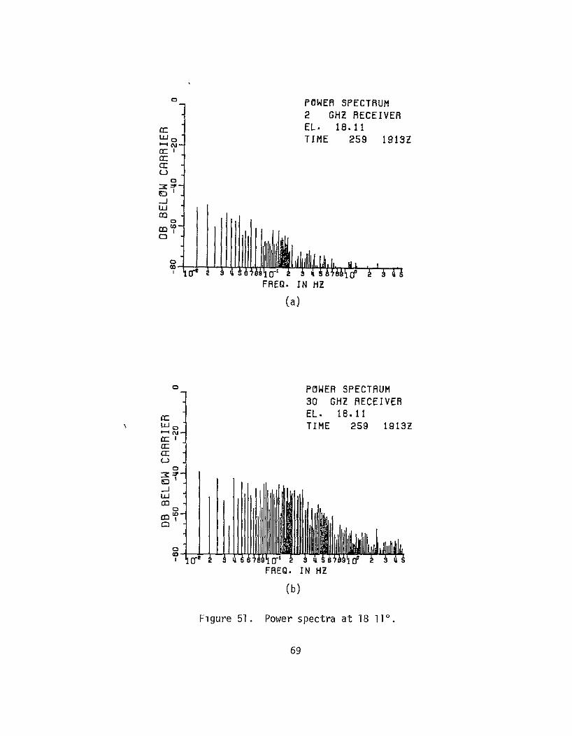
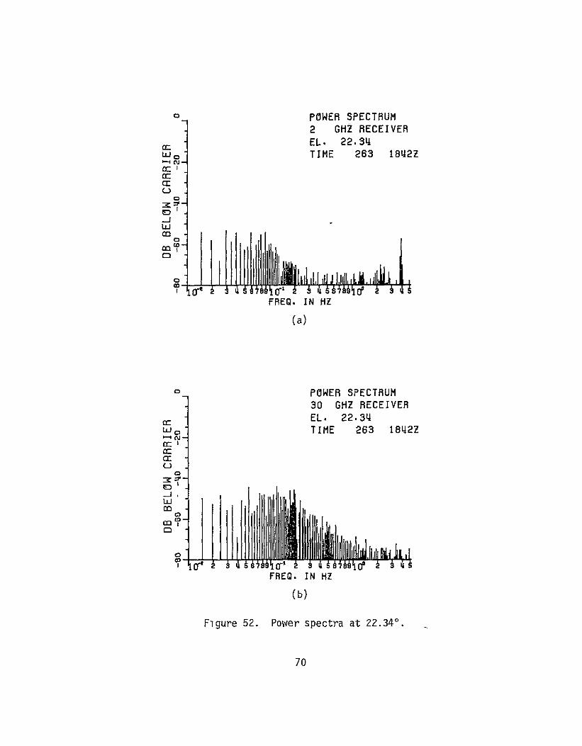
o POWER SPECTRUM
2 GHZ RECEIVER EL 2234 TIME 263 1842Z
-C
aCr
L)
CD
C
FRED IN HI (a) 0H
oPOWER SPECTRUM
30 GHZ RECEIVER EL 2234 TIME 263 1842Z
-c
m I
FREG IN HZ (b)
Figure 52 Power spectra at 2234
70
b
o POWER SPECTRUM
2 GHZ RECEIVER
EL 4389 TIME 298 1850Z
Cr
C
-J
FREQ IN HZ
Figure 53 Power spectrum at 43890
71
D Fade Distributions
Fade distributions were also studied at several elevation angles averaging about 30000 samples ie 50 minutes each Figures 54 and 55 show the percentage of time a given fade depth was exceeded plotted on a log-normal scale
The curves appear to fit fairly well within each other with increasing elevation However exceptions are clearly seen at 038 and 1600 for both 2 and 30 GHz and at 495 for the 2 GHz signal The reason for the behavior at 495 is not clear at present It should be noted that the 30 GHz fade distribution at this elevation angle does not behave in the same way
The distributions at 2820 are taken to be a representative sample for the higher elevation angle cases and show good fit to straight line approximations indicating that they are Gaussian Even the anomalous distributions show a Gaussian nature over a large portion of their ranges
The fade distributions could in fact be a combination of more than one type of statistic Deviations from the Gaussian curve are prominent for large scintillations Furthermore since the sampling rate is high (10sec) it is possible that the effects of rapid short term scintillations which are believed to be Rayleigh distributed are also being displayed in these distribution curves [28]
Assuming that the dominant long-term statistics at-the higher elevation angles are Gaussian a check was performed at 2820 as follows Let the un-normalized variance be s2 For a log-normal distribution the interval between the 50 and 999 percentile values of the cumulative distribution function - ie 50 and 01 pershycentile values of the fade distribution function - is 31 s[29] For 30 GHz from Figure 55
31 s30 = 86
=27s30
Now from the definition of a2 (Equation (3-6)) we can write that
0 ogloG2 =
dB K1
2zdB
= K110os
72
9999 FADE DISTRIBUTIONS
2 GHz 999 998 -
99 gtt
AA A
ELEVATION (DEG)
98 bull A 0
X 038 160
95 9-0D A o628228 04 A 495
90 x 0 1811 + 1+ 4381
x c0 o X
w 70 x w + E3
x 60shy
lt 50 + 40- 13
350- 0 0
C20 + x
1-0- A3 X x~
ox x 5-+ C X
+ A x X XX
2 I-
+ A
05 a
02- 0
0I 005
001 0 1 5 4 5 6 7 a 9
FADE (d8)
Figure 54 Fade distributions at 2 GHz
73
9999
999
998 -
FADE DISTRIBUTIONS
30 GHz
w w o x
99
98
95
80
A
X
x
ELEVATION (DEG)
038 x 160 0 282 A 495
1811 + 4381
600
650 a
S40 -x
w30-
-20 20
A
A x 0
10-0+D
0+ 0 5-
2--x 5
A30
Abull 0
X
0
S
X X
X OX x
2- A X
02- I A- 0 0 x
021
0010 5 10 15 20 25 30 35 40 45
FADE (d8)
Figure 55 Fade distributions at 30 GHz
74
From Figure 27 average log amplitude variance at 282
2 a ZdB 30 = - 115 dB
-115
s30 = (20 loglo e) 1 010
s30 = 234
This compares favorably with s as calculated from Figure 55
Similarly for 2 GHz at 282 from Figure 54
31 s2 = 23
= 074s2
from Figure 27 and following the same procedure as above
s2 = 045
The discrepancies could be partly due to the fact that the values shown in Figure 27 are calculated for 205 second intervals only and then averaged over each elevation angle These are therefore shortshyterm statistics and would tend to be Rayleigh distributed whereas the distributions in Figures 54 and 55 were calculated over the whole elevation angle directly these tend to be Gaussian Further the deviations from the log-normal curve for strong scintillations would also affect the result
75
CHAPTER V CONCLUSIONS
The results of the experiment are summarized in this chapter
A The Received Signals
The received siqnals show several types of fluctuations
a) Very low elevation angles (less than 40)
(i) Slow rises and fades of tens of dB over periods of tens of minutes
(ii) Faster fluctuations or scintillations with durations of a few minutes or less occurring continuously
(il) Continuous rapid scintillations of a dB or less
(iv) Slow roller-type fading is also seen However the high signal correlation found rules out ground reflection effects (Appendix D)
b) Low elevation angles (40 to 100)
(1) Very slow changes in mean level of a few dB over 30 minutes or more
(ii) Faster scintillations of several dB with periods of a few tens of seconds
(il) Continuous rapid scintillations
c) Medium elevation angles (10 - 44)
(1) Virtually no change in mean level except during precipitation events
(ii) Enhanced scintillations of a few dB for a few minutes are now visible
(iii) Continuous rapid scintillations
Scintillations were observed at all times in clear air and also in the presence of non-precipitating clouds At the highest elevation angles there appears to be a tendency for the scintillations to be enhanced in the presence of non-precipitating cumulus clouds
76
In the following discussion the symbols A and k are used to denote amplitude and log amplitude quantities respectively The symbol V is used to denote either one in general
B Variances
Amplitude and log variances are defined in Equations (3-4) and(3-6)
The range of the variances at any elevation angle exceeded 20 dB at times However the average variances followed a cosecant power law with elevation angle fairly well
Table 4
2 A [CSC(EL)] B
2 GHz 30 GHz
A B A B
10-4 9 12 162 10-4 3 214A 2 plusmn3
-43 a 2 10-49 162 10 220plusmn2 plusmn3
The fairly large error bounds have been introduced to account for the limited data Observations over extended periods under widely varying weather conditions would give a closer estimate The exponents B compare well in their range of error with the theoretical value B = 1833 for Kolmogorov type turbulence
As a refinement a spherical earth model was assumed with a uniform homogeneous atmosphere of effective height h km When this was fitted to the data the results were as follows
77
Table 5
a2 -A LB
L =Ih2 + 2hR + R2 Sin2e - RSine
R = 8479 km 0 = elevation anole
2 GHz 30 GHz
A B hkm A B hkm
10- 6 5 10- 6 4A 187 62 248 61plusmn2 plusmn1 plusmn3 plusmnI
2 10-6 4 187 61 1061 249 45
plusmn2 plusmnIt3
A reduction inmean square error of between 5 to 15 is obtained However in general the much simpler cosecant law
a A [CSC(amp)]B
appears to be quite adequate for elevation angles above 40
The 30 GHz data obtained during the departure of ATS-6 in 1975
agree well with the present data
The ratio of variances a2 1 2 has a mean value of 92 dB
A value of 44 dB was obtained for a2A30l 2A inthe 1975 measureshyments 3
C Received Signal Levels
The relative received signal levels show a strong dependence on elevation angle for elevations less than 5 They are relatively independent of elevation thereafter The drop in signal levels at low elevation angles are much greater than simple path-loss calcushylations predict
78
D Cross Correlations
Cross correlation was evaluated as a function of elevation angle Both the amplitude and log amplitude cross correlations are identical for elevations above 5 Below this angle they diverge slightly The cross correlations appear to follow a cosecant law with an exponent of 161 to 166
The average amplitude correlation was found to agree well with that predicted by Lee and Harp for the frequency ratio of 1446 The 1975 data also show good agreement with the predicted value for a frequency ratio of 15
Representative samples of auto and cross correlation functions with time lag were also shown Cross correlation lag ranged from 0 to about 10 seconds with most of the values in the region of 0 to 5 seconds Significant correlation was not found for lags exceeding 15 seconds
E Power Spectra
The power spectra of the 2 and 30 GHz signals show a characshyteristic decay with freguncy in the region of 01 to 1 Hz The roll-off follows the f- law agreeing with the assumption of tropospheric turbulence as a dominant mechanism in the samples analyzed
F Fade Distributions
Fade distributions were calculated for selected elevation angles The results suggest dominant Gaussian distributions However there is significant deviation from the normal curve for strong scintillations at low elevation angles
Fades in excess of 30 dB at 30 GHz and 7 dB at 2 GHz were observed for 5 of the time at low elevation angles These dropped to 1 dB and 06 dB respectively at 410
G Summary
Microwave signal amplitude scintillation characteristics were studied on earth-space paths for elevation angles varying from 04 to 439 using the ATS-6 satellite Beacon signals at two frequencies 2 GHz and 30 GHz were monitored simultaneously The results are consistent with similar measurements made earlier at 20 and 30 GHz
Variances are modeled well by the cosecant law and by a homoshygeneous spherical earth model with an equivalent height of 6 km Agreement with the Kolmogorov turbulence model is found The mean ratio of the variances is 94 dB
79
The correlation between the two signals was as high as 04 at low elevation angles and follows a cosecant law The average value is close to that predicted by Lee and Harp for the ratio of these frequencies Correlation lags were in the 0 - 5 second range and significant correlation was not found for lags exCeeding 15 seconds The lags may be attributed to wind fields as modeled by Lee and Harp
The power spectra at both 2 and 30 GHz show an f-8 3 roll-off in the 01 to 1 Hz range This agrees with the assumption of tropospheric turbulence as the dominant mechanism
Mean signal levels dropped sharply below predicted values at elevation angles below about 40 Fades exceeded 30 dB and 7 dB at 30 and 2 GHz respectively for 5 of the time at low elevation angles These reduced to less than I dB at an elevation of 410
The long term statistics are Gaussian except for strong scintillations when significant divergence from the Gaussian distribution was found
80
APPENDIX A EDITED TAPE FORMAT
The format of the final edited working digital magnetic tape corrected for receiver calibration characteristics is shown
Packed Tape 48 File Format
File No Day No of Records (1976)
1 243 244 38 2 245 40 3 246 247 100 4 251 254 255 47 5 257 - 263 265 266 165 6 271 18 7 275 277 281 54 8 291 292 294 296 298 70
Packed Tape 48 Record Format
Record Length = 2555 Integer words
words 1-10 = Header Wl = No of words in Record W2 = Day W3 = Hour W4 = Minute W5 = Second W6 = millisecond W7 = Azimuth (milli degrees) W8 = Elevation (milli degrees) W9 = Record Type (10 a 110 sec rate samples) W1O = Data Status
Bit = -Bit 1 = 2 GHz Rec Bit 2 = 30 GHz Rec
If receiver is on and data is usable the
corresponding bit = 1
Words 11 - 2555
Wll - W2058 max = Packed data words
in 01 dB Bits 0 - 11 2 GHz below reference IBits 12 -23 30 GHz
Remaining words are unused
81
APPENDIX B TABLE OF USEFUL DATA PERIODS
The data recorded during the experiment were edited by eliminating periods of equipment adjustment antenna peaking or adjustment and data corrupted by ground reflections at elevation angles below 038
B-I This section of the Appendix shows the periods duringwhich the data was considered usable after editing
a) Column 1
Entry number
b) Column 234
Time of day (Days Hours Minutes) Greenwich Mean Time
c) Column 56
Nominal Azimuth and Elevation angles in degrees
d) Column 78
These give the external additional attenuators in the receiver which were not directlyrecorded by the data recording system
e) Column 9
The status of the data is given in this column as an octal number as shown below
Bit no 2 1 0
Status I
Receiver 30 GHz 2 GHz 360 MHz
An acceptable data period is indicated by the corresponding bit being set to 1
82
NO OAY HOUR MIN A1 M ELEV 30 GHZ e GHZ STAT (nul (DEG) (DB) (DIR)
1 e6 10 0710l - A 14
e43 4 0 97I0 -4c4 1 1 6 37 24 -474f 6P 6 6
4 4 1 97 4F 3 o b 1b 24o4a 974F 6p 0 4 6 446 1J )2 9746 6p 1 0 7 246 19 18 97b7 45 0 6 4
8 )
a43 3L
3 it)
9763 97ol
47
47 C 0
8 b
7 r
10 2115 2L 17 9761 47 0 7
11 e45lfl -A 97b3 47 1 1 0 oe e44 bU 9eQ19 4 e 7
16 244 6 0 9819 74 0 n 5 14 244 9 50 9860 99 L 0 5
U0lb lamp
-244
i ) 1n
a 9
9AO 9830
99
99 3 b
0 1
1 4
j7 241 10 A6 9aoO 97 5 04 la 244 1ii 57 q81 5 1 1008 10 0 5
39 244 1x 30 9837 135 le 14 20 e44 IB 50 9850 154 10 3 4
244 0 I 98D9 lobO I0 2 6
22 44 41 0 959 lbO lu 2 I 26 24
45 445
1 2
54 8
9895 9P95
17017o 1030 22 27 2b e-45 6 1 9 g 95FT L7nIC 2 5
NO UAY HOUR MIN AZi M ELLV 60 GFl7 wbi$Z STAT (fLG) (DEG) (UP) (U )
4b 4 56 9913 181 1L 2 4 eL45 U 85 9913 161 0 2 5 e45 7 30 9p2 196 10 2 5
29 e45 9 20 99e2 196 10 2 4 3U =45 9 4u 99e7 211 ILI 2 5 31 11 4b50 90e7 211 16 2 U 52 24b 12 O 9941 21 3 I 5 36 245 13 15 9931 P63 i( 2 4 -4 c45
45 It 14
0 3Q
9961 99 54
263 247
IG IC
2
4 4
o6 d45 16 30 3 9 22b7 10 2 4 37 245 lb M1 9q47 b6 IC 2 4 38 245 z 6 9b6 271 10 2 6 35 40
45 e46
21 1
U 54
9b6 9994
71 26p
IC 10
2 2
0 7
41 246 0 9994 282 10 2 5 12 e46 4 U 100116 p6C 10 2 5 41 246 5 6 10006 28q 10 2 7 L4 246 b U 30f06 289 10 2 fl I b 6 17 4 10040 72 10 2 6 46 246 IS 4 10040 37 10 4 u7 246 19 U 3Lin Q $7 1 2 4 48 246 2C 4 10054 --82 I0 2 6
ee46 21 U 1On54 Ab2 10 2 4 50 a46 21 30 lO0Dt 6b2 10 2 0
NO UAY HOUR IIN AZI fuI ELEV 60 GIZ 2 bHZ STAT (DEG) (PLG) (DP) (Or)
51 47 b 9 10136 474 22 2 6 52 247 16 10153 474 22 2 4 So d47 17 U 30133 483 22 2 4 594 247 je 54 10147 491 22 2 5 95 e4 7 0 19 101 bE 495 22 2 7 5( 247 21 2 101b59 495 22 2 0 57 248 16 55 10268 594 22 2 5 58 248 19 U 10247 602 22 2 0 59 251 j7 4 10545 92c) 1) 7 60 ebl 17 2U 10545 929 2 0 0 61 e54 11 6 10850 1222 22 0 7 62 254 12 95 1P50 12e2 22 6 66 e 32 n UPSbU 1222 amp2 0 7 64 254 12 30 XOU50 1222 2 0 0 65 e55 15 34 10a67 16b3 22 0 7 66 255 16 25 10q67 163 22 0 0 67 e57 23 5 ltf 156 22 0 7 f6 eb7 14 U 111L 1t65 22 0 o 69 258 36 11316 17o4 22 0 6
r70 258 19 50 11316 1704 22 0 0 71 259 18 31 l11o2 1811 22 0 72 259 19 30 31462 1811 2a 0 0 76 260 19 29 11550 1918 22 0 6 74 260 19 26 11551 1918 22 0 4 7t 260 19 27 11550 1918 22 2 6
N10 DAY HOUR MIN AziM1 ELEV O GH2 2 6H7 STAT ( Lu ( Lu) (OH) (UU)
76 260 19 51 11 0 19018 22 2 0 77 261 i6 31 1r453 1998 22 7b e61 IN 31 111453 1998 2 2 u 79 262 2 118G3 r216 22 2 E bu 61 20 59 l1v 263 0 Pl 266 1A 19 1117 2264 22 2E 82 263 19 40 llq17 2234 1 2
86 e65 49 12a V 2416 P2 2 6
84 265 14 30 12158 2416 2 2 0 pound5 2E6 i1 1 122~v a 3t4 dc -
86 e7
266 266
16 -14
37 1
1228Q 12LP39
2r14 5o1
22 2
2 U
86 266 14 30 1226 2514 e2 0 8 271 4 52 12922 2923 22 0 6 9 e7 Q 1 2 94e 2SZ3 22 0 0 91 e71 4 66 1C942 2c3 22 6 92 eTi 5 51 1292 2926 22 2 0 96 e5 17 06 166i0 33br 22 2 6 94 475 18 50 ii0 53b 22 2 0 95 e77 2U 52 13972 653 2 2 96 277 21 56 15972 3566 22 P 0 q7 281 1 )I 144kj ULu2 22 2 6 9 t 281 1 41 14641 5 02 2e 2 0 99 291 2U b 14764 4aiq 22 2 6
IOU eql 21 0 167a 4119 22 2 U
NO t AY HOUR MIN AZIN ELEV 30 GHZ 2 GHZ STAT (uEb) (WEG) (08) (JB)
101 e92 l 5 169 16 44 22 6 102 292 19 15 16076 43Q44 22 2 0 106 94 C 55 17278 63A 22 b 14 2994 6 30 1727P 413A 22 2 0
105 296 134 27n414 4381 2 C 1o6 96 15 0 1784 4361 22 2 0 In d98 1e 20 18342 4389 22 2 6 lob 98 19 0 18342 43a9 22 2 0
B-2 The durations of the data periods used in the calculations in this report are given below
Elevation (degrees)
038 048 074 160 170 271 282 289 372 382 474 495
929 1222 1363 1565
Duration (minutes)
32 19 20 46 71 57 61 57 60 56 52 42
16 84 54 57
Elevation (degrees)
1704 1811 1918 1998 2135 2234 2416 2514 2923 3365 3536 3802
4319 4344 4358 4381 4389
Duration (minutes)
54 59 81 59 57 71 41 50 57 57 57 56
52 57 35 66 40
OF POOR QUPLrfORIG19M FAOt 1S
88
APPENDIX C COMMENTS ON LOG AND AMPLITUDE VARIANCE
Expanding the definition of log variance (Equation (3-6))
N 12NN2 1 1a = iL-- I~N 1 kJ KIN i=1( l 22
2 1 N a
= (120 log101 0a 20 lOgio (C-1)
K2N 11 a0 NJ 2 1091 ) 10
but
a a lglO a9 l - + lg0 ashy
0 a o
N a2 202 N O - 1 1oq 0 -- + loK10 To - logl - +10
K1IN i=1(I a o yl
a09lt2N aya
KaN1 20 10
20 Y2 1
1090 logoeK =a I a
Kl = lOg0 e loge
a a
2 a N
a_Y (20 loglo -_1I N I loge l 2 2 (20 logloe)2
(20 logloe) I a j=1 a
89
For small scintillations a
a 1
lo e = - Jrl
Also
2 1 Cf
ala
(a 1 1
a) (C-2)
2= N a
ao
2 N (a shy T)2
2 - 02(-3)
2 a2 for small scintillations
The computed results show excellent agreement even at low elevation angles (ie large scintillations)
Further Fried has shown [30] from energy considerations that
a2p _-T (C-4)
(This result has been adapted to be consistent with the definitions used in this study)
90
0
Now Z shows a sharp drop at low elevat~o9 angles It seen n Figure 56 where the numerical values of K1 a z(NB not pounddB
are plotted that this behavior is in fact reflected
The observations are therefore consistent However the reason for the sharp knee in the mean levels is yet to be determined
LOG-VRRIRNCE
+ 2 GHz
x 30 GHz
x2 IX)2
ci X X
CD
x
+
5 10 15 20 25 30 35 40 45 ELEV (DEG)
Figure 56 Log amplitude variance (numeric)
91
APPENDIX D RECEIVED SIGNALS AT LOW ELEVATION ANGLES
AND MULTIPATH EFFECTS
The mechanism which causes the amplitude scintillations may be regarded as being either refractive or multipath in nature Low two-frequency correlation would be expected if multipath were the dominant factor because an arbitrary differential path length cannot produce simultaneous subtractive or additive phasing at the two wavelengths employed as shown below [17]
Subtractive multipath phasing will occur at a wavelength of X1 if the difference between the two path lengths satisfy
AL = (2n+l) -7 n = O 2
Similarly at a second wavelength X2
AL = (2m+l) 2p m = 0 1 2
Therefore
(2n+l)A 1 = (2m+l)A 2
But in general
A I = PA2 where P is an arbitrary number
So that
P(2n+l) = 2m+l (D-1)
For example the 1975 measurements were performed simultaneously at 20 and 30 GHz therefore P = 32 Then
3 (2n+l) = 2m+l
or 3(2n+l) = 2(2m+l) (D-2)
However the left side of Equation (D-2) is odd and the right side is even Therefore simultaneous fading due to simple multishypath propagation cannot occur This result contradicts the very high correlations observed between the 20 and 30 GHz signal fluctuations Thus one is forced to conclude that the observed fluctuations are not a result of a simple multipath mechanism
92
APPENDIX E SUMMARY OF DEFINITIONS
a(t) is a positive real signal amplitude a are discrete samples of a(t) at equal intervals over a time interval T a(t) has been corrected for receiver nonlinearities The relative amplitudeis defined to be
a A =- I I a0
and the relative log amplitude as
20 logO ashy=
where a0 is an arbitrary constant
93
AMPLITUDE LOG AMPLITUDE RELATIONSHIP FORSMALL SCINTILLATIONS
= _ A(t) dt = fT1 (t) dt
MEAN JT d z J T N t T 20 loglo
1= 1 L1=1
MEAN TOTAL POWER I JA2(t) t (MEAN SQUARE) N 2 A vdBz
N i1I
VARIANCE ~ (NORMALIZED TO DC POWER)
2 AT
1jf A(t+i2 A N
dt 2 1 T
Wtd NaAC
2-22
NA 1 1 KNK~I 1lN1=
AMPLITUDE LOG AMPLITUDE
CORRELATION
COEFFICIENT
12 --I (Am (t)-l)(A2 (t+T)-T 2 )dt
PA(t)T Al- O 0A1 A1I[2
(A 2- A-I2 I (A (A2 A2 )
1N=l2 0= A1 A2
2 1 z(t)-T( t+r)-12 )dt
f 2K1l 2
1I2
N ( lI- -I)( 21+j- 2) 1 )
K1N 1=] lP2
RELATIONSHIP FOR SMALL SCINTILLATIONS
PA12 v 2
K 20 logloe T = j T IT
REFERENCES
[1] L Cuccia W Quan and C Hellman Above 10 GHz Satcom Bands Spur New Earth Terminal Development Microwave System News March 1977 p 3738
[2] L Cuccia et al Op Cit p 46-50
[3] D E Kerr Propagation of Short Radio Waves McGraw Hill 1964
[4] B R Bean and E J Dutton Radio Meteorology Dover 1968
[5] D C Livingston The Physics of Microwave Propagation Prentice Hall 1970
[6] Propagation Factors in Space Communications AGARD Conference Proceedings No 3 W J Mackay and Co 1967
[7] P David and J Voge Propagation of Radio Waves Pergamon Press 1969
[8] Communications Satellite Corporation COMSAT Technical Review Vol 3 No 1 to Vol 5 No 2
[9] E V Appleton URSI Proceedings Washington 1927
[10] E H Whitney and S Basu The Effect of lonosphereic Scintillation on VHFUHF satellite Communications Radio Science Vol 12 No 1 1977 p 123-133
[11] Aarons et al Radio Astronomy Measurements at VHF and Microwaves Proceedings IRE January 1958 p 325-333
[12] L A Hoffman et al Propagation Observations at 32 Millishymeters Proceedings IEEE Vol 54 No 4 April 1966
[13] L J Ippolito Effects of Precipitation on 153 and 3165 GHz Earth-Space Transmission With the ATS-V Satellite Proceedings IEEE Vol 59 No 2 1971
[14] L J Ippolito ATS-6 Millimeter WaVe Propaqation and Communishycations Experiments at 20 and 30 GHz IEEE Transactions Vol AES-ll No 6 1975
[15] Goddard Space Flight Center ATS-F and -G Data Book September 1972 p A39-A42
96
[16] D B Hodge and D M Theobold Scintillations Observed on the ATS-6 20 and 30 GHz Downlinks URSIUSNC meeting Boulder Colorado October 1975
[17] D B Hodge D M Theobold and R C Taylor ATS-6 Millimeter Wavelength Propagation Experiment Report 3863-6 January 1976 The Ohio State University ElectroScience Laboratory Department of Electrical Engineerng prepared under Contract NAS5-21983 For NASA Goddard
[18] V I Tatarski Wave Propagation in a Turbulent Medium Israel Program for Scientific Translation Jerusalem 1971
[19] R F F11ipowski and E I Muehldorf Space Communication Systems Prentice Hall 1965
[20] G N Krassner Introduction to Space Communication Systems Chapter 4 McGraw Hill 1964
[21] D M Theobold and D B Hodge ATS-6 Millimeter Wavelength Propagation Experiment Report 3863-4 April 1975 The Ohio State University ElectroScience Laboratory Department of Electrical Engineering prepared under Contract NAS5-21983 for NASA Goddard
[22] B H Briggs and I A Parkin On The Variation of Radio Star and Satellite Scintillations with Zenith Angle J Atmos Terr Phys 25 p 339-366
[23] A Kolmogorov Turbulence Classic Papers on Statistical Theory S K Friedlander and L Topper Eds New York Interscience 1961 p 151
[24] A Benoit Signal Attenuation Due to Neutral Oxygen and Water Vapor Rain and Clouds The Microwave Journal November 1968 p 73-80
[25] K S McCormick and L A Maynard Measurements of SHF Tropospheric Fading Along Earth-Space Paths at Low Elevation Angles Electronics Letters Vol 8 1972 p 274
[26] R W Lee and J C Harp Weak Scattering in Random Media with Applications to Remote Probing Proc IEEE Vol 57 1969 p 375-406
[27] R S Lawrence and J W Strohbehn ASurvey of Clear Air Propagation Effects Relevent to Optical Communications Proc IEEE Vol 58 No 10 October 1970 pp 15371538
97
[28] P F Panter Com unication Systems Design McGraw Hill 1972
pp 347-358
[29] P F Panter Op Cit p 355
[30] D L Fried Optical Resolution Through a Randomly Inhomoshygeneous Medium for Very Long and Very Short Exposures J Opt Soc Am 56 October 1966 pp 1372-1379
98
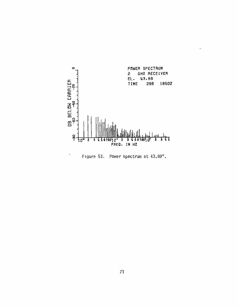
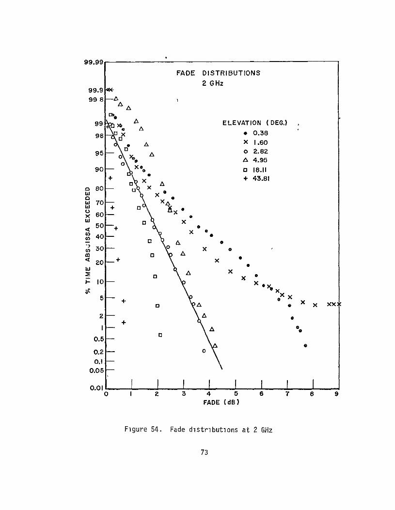
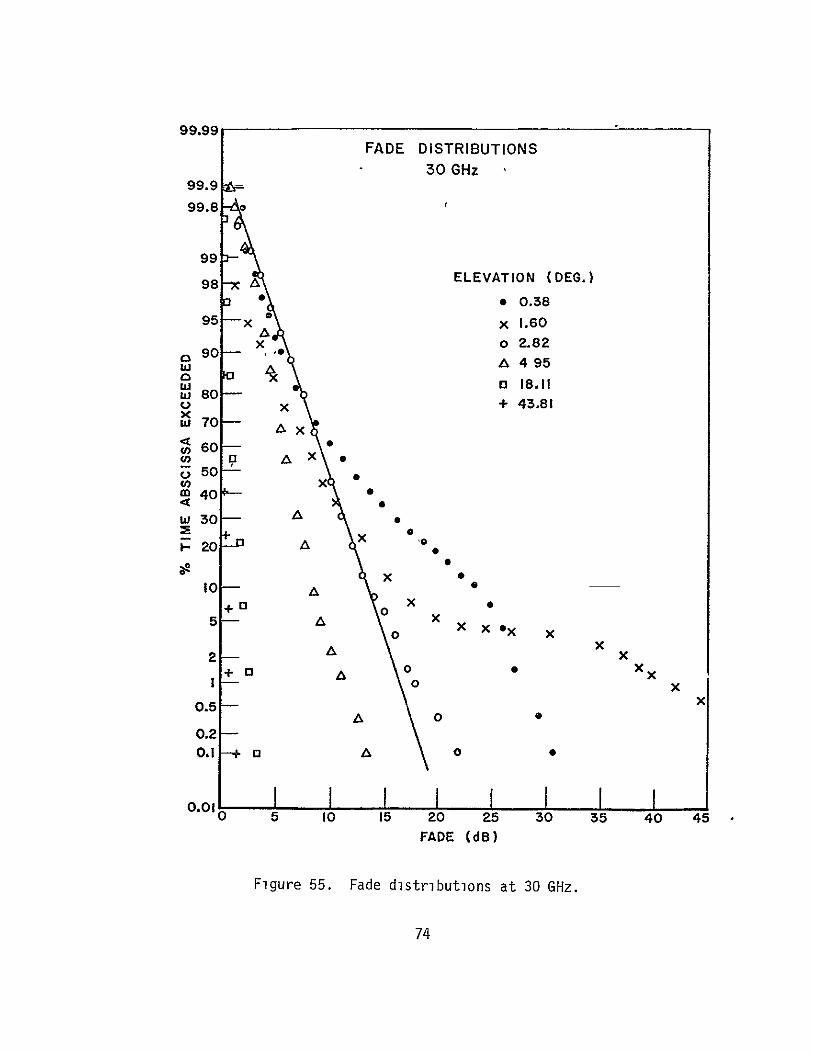
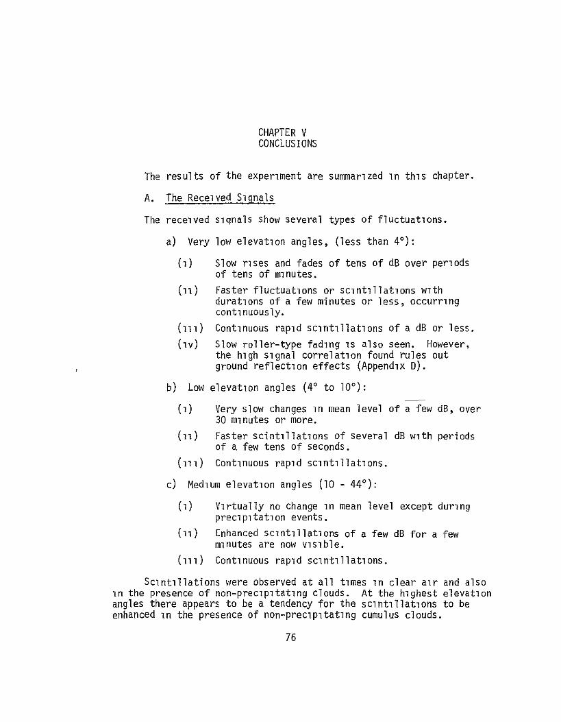
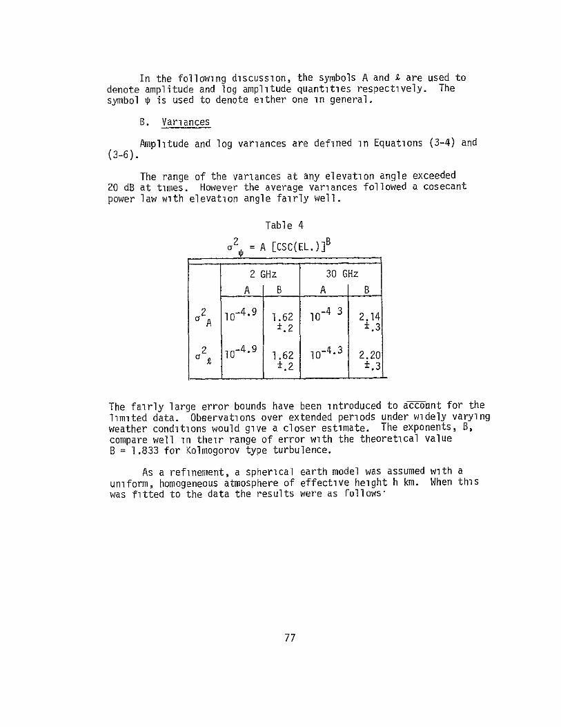
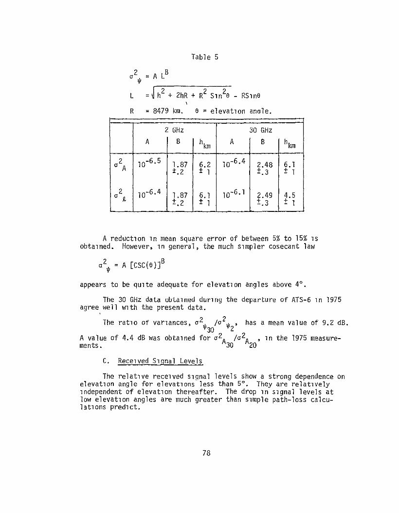
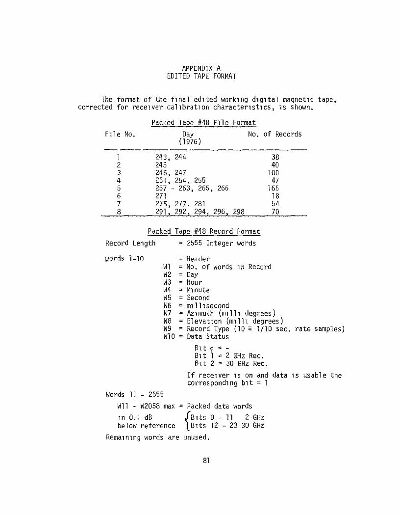
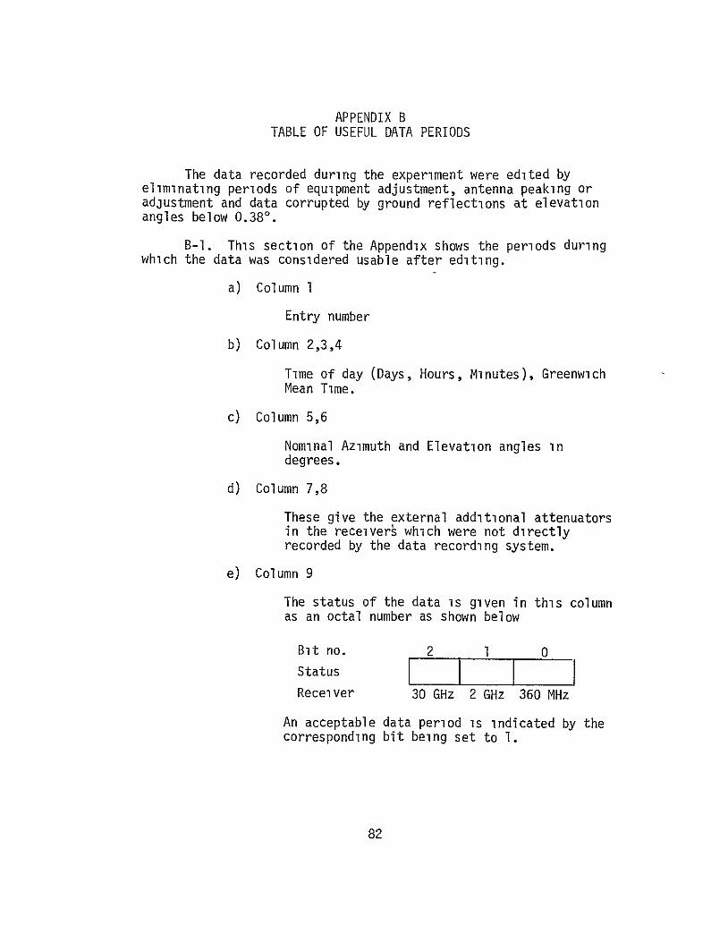
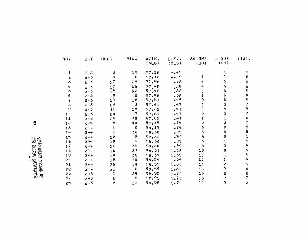
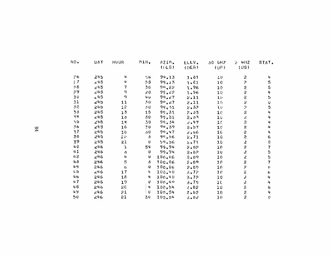
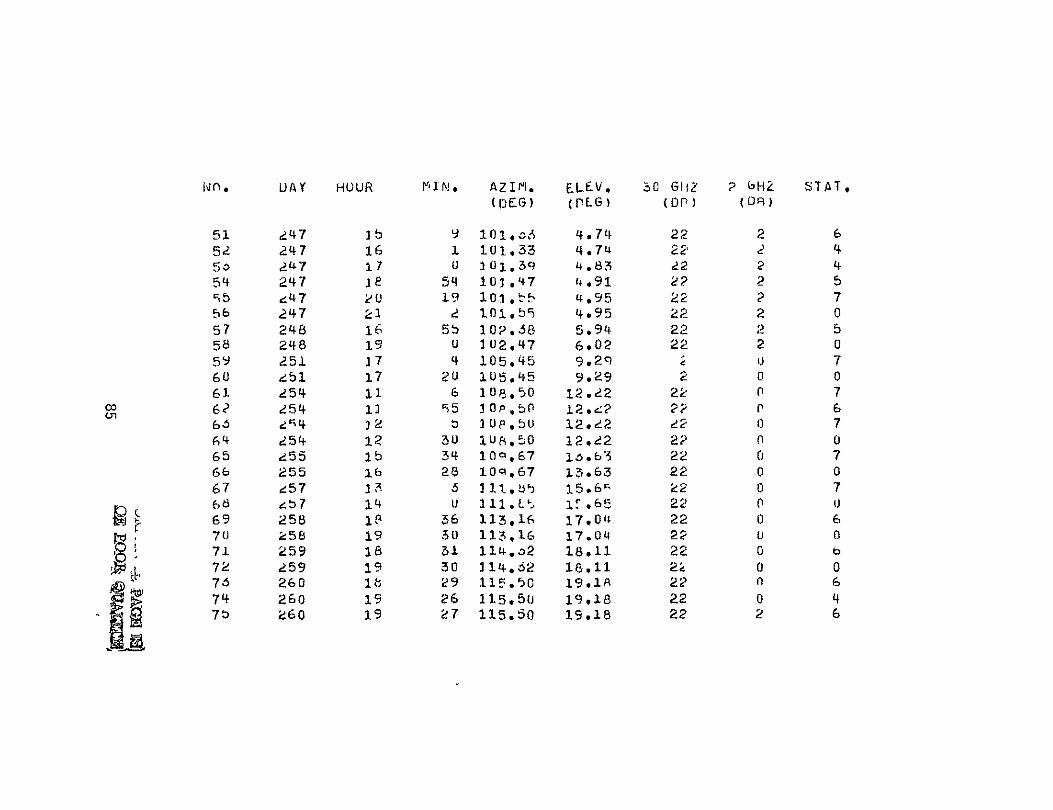
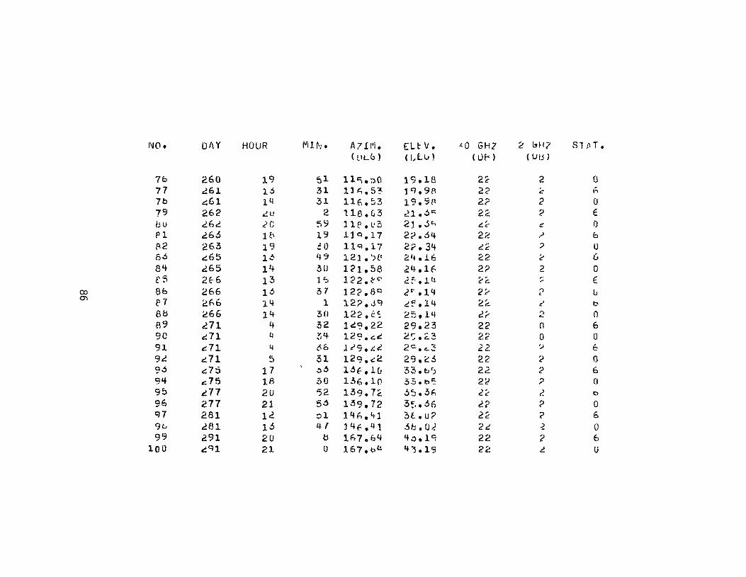
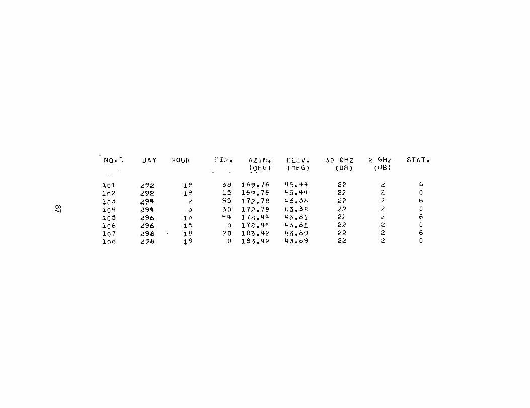
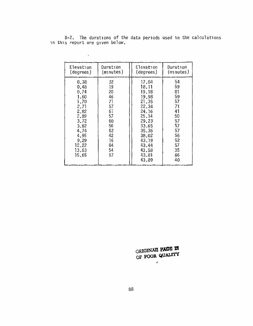
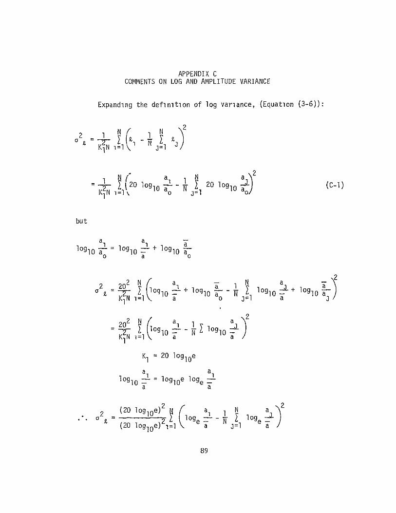
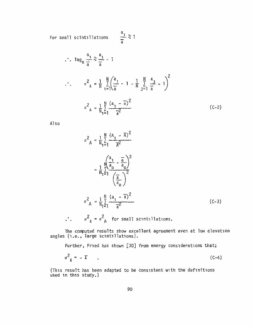
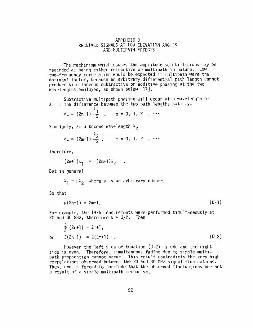
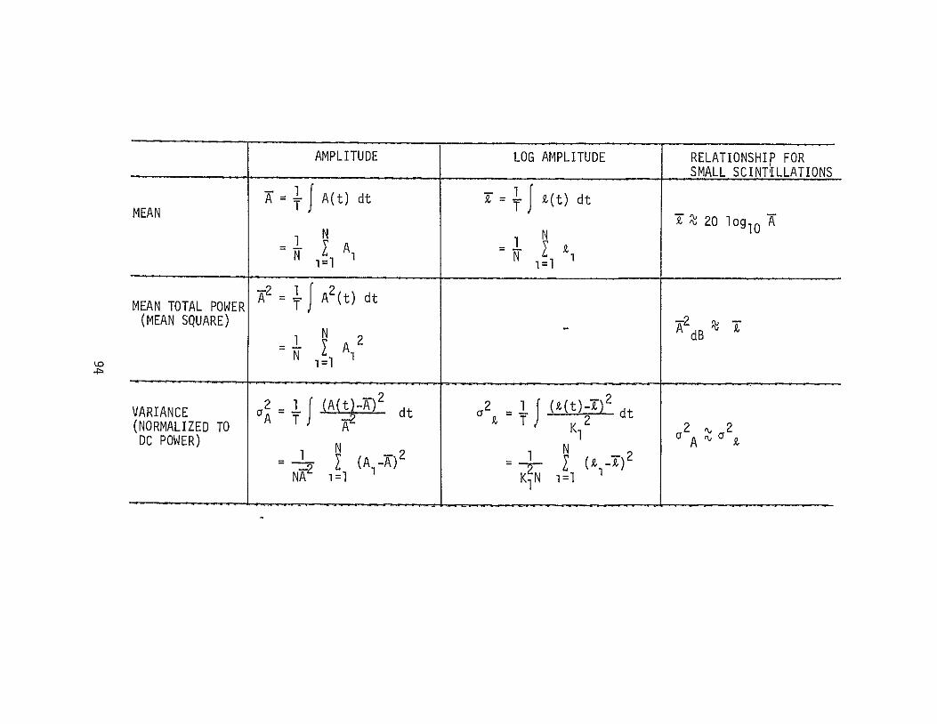
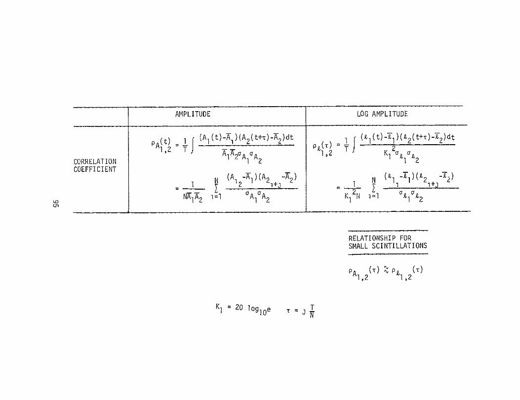
[28] P F Panter Com unication Systems Design McGraw Hill 1972
pp 347-358
[29] P F Panter Op Cit p 355
[30] D L Fried Optical Resolution Through a Randomly Inhomoshygeneous Medium for Very Long and Very Short Exposures J Opt Soc Am 56 October 1966 pp 1372-1379
98
Related Documents


