Electromagnetic Fast-transients in LV Networks with ...

Electromagnetic Fast-transients in LVNetworks with Ubiquitous Small-scale

Embedded Generation

David A. Clark

Thesis submitted to Cardiff Universityfor the degree of Doctor of Philosophy

30th March , 2012

Abstract

Small-scale embedded generation projects rated below 16A per phase are being integrated

into low-voltage distribution networks in ever increasing numbers. Seen from the

network operator’s perspective as little more than negative load, the commissioning of

such generators is subject to compliance with the Fit and Forget connection requirements

of ENA Engineering Recommendation G83/1. This thesis has sought to quantify the

electromagnetic switching transient implications of integrating very large volumes of

embedded generation into the UK’s low-voltage supply networks.

Laboratory testing of a converter-interfaced PV source has been undertaken to

characterise typical switching transient waveshapes, and equivalent representative source

models have been constructed in EMTP-ATP. A detailed frequency-dependent travelling

wave equivalent of the DNO-approved Generic UK LV Distribution network model

has been developed and, by means of extensive statistical simulation studies, used

to quantify the cumulative impact of geographically localised generators switching in

response to common network conditions.

It is found that the magnitude of generator-induced voltage and current transients

is dependent on the number of concurrently switched generators, and on their relative

locations within the network. A theoretical maximum overvoltage of 1.72pu is predicted

at customer nodes remote from the LV transformer terminals, for a scenario in which

all households have installed embedded generation. Latent diversity in switch pole

closing and inrush inception times is found to reduce predicted peak transient voltages

to around 25-40% of their theoretical maxima.

i

Acknowledgements

This work was carried out within the High-Voltage Energy Systems (HIVES) Research

Group, Institute of Energy, Cardiff School of Engineering between October 2007 and

March 2012.

Thanks are due first and foremost to Prof. Manu Haddad and Dr. Huw Griffiths for

their supervision and guidance, without which this work would not have been possible.

Sincere thanks are also due to Prof. Noel Schulz for her invaluable input while on

sabbatical from Mississippi State University.

Experimental work was undertaken in the Cardiff University Solar Energy Laboratory

under the guidance of Dr. Anthony Giles and with assistance of the school’s technical

staff, principally Mr. Paul Farrugia, Mr. Steve Mead, Mr. Mike Baynton, Mr. Alan Jauncey,

Mr. Denley Slade, Mr. Richard Rogers and Mr. David Glinn. With regard to supporting

EMTP simulation work, the author would like to acknowledge the invaluable expertise

of his colleagues Dr. Maurizio Albano, Mrs. Haziah Abdul Hamid, Mr. Stephen Robson

and Mr. Fabian Moore.

Thanks are also due to Prof. Nicholas Jenkins, Dr. Noureddine Harid, Dr. Dongsheng

Guo, Dr. Liana Cipcigan, Dr. Jun Liang, Dr. Bieshoy Awad, Mr. Steve Watts, Mr. Alexander

Bogias and Mr. Ahmed El-Mghairbi for their advice and input throughout this project.

Finally, I would like to thank my family for their patience and encouragement throughout

my time at Cardiff.

ii

List of Publications

Conference

D. Clark, A. Haddad, and H. Grffiths,“Switching transient analysis of small distributed

generators in low voltage network”, CIRED 2009. 20th International Conference and

Exhibition on Electricity Distribution - Prague, Czech Republic, June 2009.

D. Clark, A. Haddad, H. Griffiths, and N. N. Schulz, “Analysis of switching transients in

domestic installations with grid-tied microgeneration”, North American Power Symposium

(NAPS) - Starkville, MS, October 2009.

Journal

D. Clark, A. Haddad, H. Griffiths,“A laboratory test facility for the evaluation switching

transients in small-scale embedded generators”, In progress, expected submission for

review: Autumn 2012

D. Clark, A. Haddad, H. Griffiths, “A generic model for determining electromagnetic

transient propagation in low voltage supply networks”, In progress, expected submission

for review: Autumn 2012

iii

Contents

Abstract i

Acknowledgements ii

List of Publications iii

Contents ix

List of Figures xiv

List of Tables xvi

List of Abbreviations xvii

List of Mathematical Symbols xix

Hypothesis 1

Introduction 2

Chapter Summaries . . . . . . . . . . . . . . . . . . . . . . . . . . . . . . . . 5

1 Literature Review 7

1.1 UK Microgeneration Prospects . . . . . . . . . . . . . . . . . . . . . . . 81.1.1 Small-scale Embedded Generation - A Definition . . . . . . . . . 91.1.2 Adoption Scenarios . . . . . . . . . . . . . . . . . . . . . . . . . . 10

1.2 Embedded Generation Technologies and Their Impact on System Performance. . . . . . . . . . . . . . . . . . . . . . . . . . . . . . . . . . . . . . . . . 12

1.2.1 Source Types . . . . . . . . . . . . . . . . . . . . . . . . . . . . . 121.2.1.1 Photovoltaics . . . . . . . . . . . . . . . . . . . . . . . . 121.2.1.2 Wind . . . . . . . . . . . . . . . . . . . . . . . . . . . . 141.2.1.3 Small Hydro . . . . . . . . . . . . . . . . . . . . . . . . 161.2.1.4 MicroCHP . . . . . . . . . . . . . . . . . . . . . . . . . 171.2.1.5 Developing Technologies . . . . . . . . . . . . . . . . . . 19

1.2.2 Interfaces . . . . . . . . . . . . . . . . . . . . . . . . . . . . . . . 191.2.3 Impact on Grid Operation . . . . . . . . . . . . . . . . . . . . . . 20

1.2.3.1 Power Flows . . . . . . . . . . . . . . . . . . . . . . . . 211.2.3.2 Voltage Control . . . . . . . . . . . . . . . . . . . . . . 241.2.3.3 Losses . . . . . . . . . . . . . . . . . . . . . . . . . . . . 281.2.3.4 Additional Considerations . . . . . . . . . . . . . . . . . 30

1.3 Transients in Low-Voltage Systems . . . . . . . . . . . . . . . . . . . . 321.3.1 Transient Measurement Studies . . . . . . . . . . . . . . . . . . . 321.3.2 Surge Propagation and LV Transient Suppression . . . . . . . . . 34

iv

1.3.3 Power Quality Implications of SSEG . . . . . . . . . . . . . . . . 34

1.4 Time-Domain LV Network Simulation . . . . . . . . . . . . . . . . . . . 351.4.1 General . . . . . . . . . . . . . . . . . . . . . . . . . . . . . . . . 361.4.2 Cable and Line Modelling . . . . . . . . . . . . . . . . . . . . . . 371.4.3 Transformers . . . . . . . . . . . . . . . . . . . . . . . . . . . . . 411.4.4 Relays and Circuit Breakers . . . . . . . . . . . . . . . . . . . . . 421.4.5 Pertinent Studies . . . . . . . . . . . . . . . . . . . . . . . . . . . 42

1.5 Relevant Standards . . . . . . . . . . . . . . . . . . . . . . . . . . . . . 43

1.6 Chapter Summary . . . . . . . . . . . . . . . . . . . . . . . . . . . . . . 44

2 Time-Domain Simulation Suitable for Low-Voltage Systems 45

2.1 Overview of Time-Domain Simulation . . . . . . . . . . . . . . . . . . . 45

2.2 Numerical Solution of Electromagnetic Transients . . . . . . . . . . . . . 472.2.1 The Trapezoidal Rule and Linear Circuits . . . . . . . . . . . . 47

2.2.1.1 Accuracy of Solution . . . . . . . . . . . . . . . . . . . 482.2.1.2 Stability . . . . . . . . . . . . . . . . . . . . . . . . . . 492.2.1.3 Conditioning . . . . . . . . . . . . . . . . . . . . . . . . 49

2.2.2 Non-linear Components . . . . . . . . . . . . . . . . . . . . . . . 502.2.2.1 Non-linear Inductors . . . . . . . . . . . . . . . . . . . . 512.2.2.2 Hysteresis Modelling . . . . . . . . . . . . . . . . . . . . 522.2.2.3 Non-linear Resistance . . . . . . . . . . . . . . . . . . . 52

2.2.3 Transmission Lines . . . . . . . . . . . . . . . . . . . . . . . . . . 532.2.3.1 Frequency Dependent Transmission Lines . . . . . . . . 542.2.3.2 Modal Domain Model (J. Martı) . . . . . . . . . . . . . 552.2.3.3 Phase Domain Model (Noda) . . . . . . . . . . . . . . . 57

2.3 Special Considerations in LV Networks . . . . . . . . . . . . . . . . . . . 582.3.1 Distance and Time . . . . . . . . . . . . . . . . . . . . . . . . . 582.3.2 Conductor Geometry . . . . . . . . . . . . . . . . . . . . . . . . . 602.3.3 Insulation Materials . . . . . . . . . . . . . . . . . . . . . . . . . 632.3.4 Insulation Coordination . . . . . . . . . . . . . . . . . . . . . . . 63

2.4 LV Distribution Network Components . . . . . . . . . . . . . . . . . . . 632.4.1 Basis in Generic Models . . . . . . . . . . . . . . . . . . . . . . . 632.4.2 Cables . . . . . . . . . . . . . . . . . . . . . . . . . . . . . . . . 632.4.3 Overhead Lines . . . . . . . . . . . . . . . . . . . . . . . . . . . 652.4.4 Transformers . . . . . . . . . . . . . . . . . . . . . . . . . . . . . 652.4.5 Switchgear . . . . . . . . . . . . . . . . . . . . . . . . . . . . . . 662.4.6 System Equivalent Impedance . . . . . . . . . . . . . . . . . . . . 66

2.5 Domestic/Commercial Wiring Installations . . . . . . . . . . . . . . . . 672.5.1 Cables and Distribution Boards . . . . . . . . . . . . . . . . . . 672.5.2 Loads . . . . . . . . . . . . . . . . . . . . . . . . . . . . . . . . . 68

2.6 Small-scale Embedded Generation . . . . . . . . . . . . . . . . . . . . . 692.6.1 Direct Connection . . . . . . . . . . . . . . . . . . . . . . . . . . 692.6.2 Converter Interfaces . . . . . . . . . . . . . . . . . . . . . . . . . 692.6.3 Switches and Disconnects . . . . . . . . . . . . . . . . . . . . . . 69

2.7 Chapter Conclusions . . . . . . . . . . . . . . . . . . . . . . . . . . . . . 69

v

3 Laboratory Rig for the Evaluation of Microgeneration TransientPhenomena 71

3.1 Overview . . . . . . . . . . . . . . . . . . . . . . . . . . . . . . . . . . . 71

3.2 Test and Equipment Specification . . . . . . . . . . . . . . . . . . . . . . 723.2.1 Time-Domain I-V Measurement . . . . . . . . . . . . . . . . . . 723.2.2 Test Scenarios . . . . . . . . . . . . . . . . . . . . . . . . . . . . 763.2.3 Statistical Analyses . . . . . . . . . . . . . . . . . . . . . . . . . 773.2.4 Repeatability . . . . . . . . . . . . . . . . . . . . . . . . . . . . . 77

3.3 The Solar Energy Laboratory . . . . . . . . . . . . . . . . . . . . . . . . 783.3.1 Lamps . . . . . . . . . . . . . . . . . . . . . . . . . . . . . . . . . 783.3.2 Ignition and Control . . . . . . . . . . . . . . . . . . . . . . . . . 803.3.3 Orientation and Manoeuvrability . . . . . . . . . . . . . . . . . . 81

3.4 Photovoltaic Array Test Rig . . . . . . . . . . . . . . . . . . . . . . . . 823.4.1 Panels . . . . . . . . . . . . . . . . . . . . . . . . . . . . . . . . . 823.4.2 Inverter . . . . . . . . . . . . . . . . . . . . . . . . . . . . . . . . 83

3.5 Test and Measurement Equipment . . . . . . . . . . . . . . . . . . . . . 853.5.1 Steady-State Monitoring . . . . . . . . . . . . . . . . . . . . . . . 85

3.5.1.1 Probes and Meters . . . . . . . . . . . . . . . . . . . . . 853.5.1.2 Data-acquisition Board . . . . . . . . . . . . . . . . . . 86

3.5.2 Fast Transient Measurement . . . . . . . . . . . . . . . . . . . . 863.5.2.1 Voltage Probes . . . . . . . . . . . . . . . . . . . . . . . 863.5.2.2 Current Probes . . . . . . . . . . . . . . . . . . . . . . . 873.5.2.3 Scope . . . . . . . . . . . . . . . . . . . . . . . . . . . . 87

3.6 Data Acquisition . . . . . . . . . . . . . . . . . . . . . . . . . . . . . . . 873.6.1 Requirements . . . . . . . . . . . . . . . . . . . . . . . . . . . . . 883.6.2 Program Overview . . . . . . . . . . . . . . . . . . . . . . . . . . 88

3.6.2.1 Inputs . . . . . . . . . . . . . . . . . . . . . . . . . . . . 883.6.2.2 Execution . . . . . . . . . . . . . . . . . . . . . . . . . . 89

3.6.3 DAQ Program Execution Structure . . . . . . . . . . . . . . . . 903.6.4 Data Files . . . . . . . . . . . . . . . . . . . . . . . . . . . . . . . 91

3.7 Data Post-processing . . . . . . . . . . . . . . . . . . . . . . . . . . . . . 933.7.1 Rising Edge . . . . . . . . . . . . . . . . . . . . . . . . . . . . . . 943.7.2 Falling Edge . . . . . . . . . . . . . . . . . . . . . . . . . . . . . 953.7.3 Energy Measure . . . . . . . . . . . . . . . . . . . . . . . . . . . 953.7.4 Energy Content . . . . . . . . . . . . . . . . . . . . . . . . . . . . 963.7.5 Switch/Inrush Timing and Delay . . . . . . . . . . . . . . . . . . 96


4 Statistical Switching Transient Measurements of a Solar EnergyInverter Source 100

4.1 Background . . . . . . . . . . . . . . . . . . . . . . . . . . . . . . . . . . 100

4.2 Laboratory Test Configurations . . . . . . . . . . . . . . . . . . . . . . . 1014.2.1 Transients on Generator Reconnection . . . . . . . . . . . . . . . 1014.2.2 Effect of Supply Impedance on Voltage Peak . . . . . . . . . . . 1024.2.3 Transients on Generator Disconnection . . . . . . . . . . . . . . . 103

4.3 Experimental Results . . . . . . . . . . . . . . . . . . . . . . . . . . . . . 1034.3.1 Statistical Measures . . . . . . . . . . . . . . . . . . . . . . . . . 104

4.3.1.1 Skewness . . . . . . . . . . . . . . . . . . . . . . . . . . 1044.3.1.2 Kurtosis . . . . . . . . . . . . . . . . . . . . . . . . . . 104

vi

4.3.2 Current Transients . . . . . . . . . . . . . . . . . . . . . . . . . 1054.3.2.1 Peak Measurements . . . . . . . . . . . . . . . . . . . . 1064.3.2.2 Current Rate of Change . . . . . . . . . . . . . . . . . . 1074.3.2.3 Timing Dependence . . . . . . . . . . . . . . . . . . . . 1114.3.2.4 Waveshape Analysis . . . . . . . . . . . . . . . . . . . . 112

4.3.3 Voltage Transients . . . . . . . . . . . . . . . . . . . . . . . . . . 1154.3.3.1 Peak Measurements . . . . . . . . . . . . . . . . . . . . 1154.3.3.2 Voltage Rate of Change . . . . . . . . . . . . . . . . . . 1174.3.3.3 Waveshape Analysis . . . . . . . . . . . . . . . . . . . . 119

4.3.4 Switch Timing . . . . . . . . . . . . . . . . . . . . . . . . . . . . 1214.3.4.1 Pole Angle . . . . . . . . . . . . . . . . . . . . . . . . . 1214.3.4.2 Switch / Inrush Delay . . . . . . . . . . . . . . . . . . . 121

4.3.5 Transient Energy . . . . . . . . . . . . . . . . . . . . . . . . . . . 1214.3.5.1 Current Transient Energy Measure . . . . . . . . . . . . 1234.3.5.2 Voltage Transient Energy Measure . . . . . . . . . . . . 1234.3.5.3 Waveform Energy Content . . . . . . . . . . . . . . . . 125

4.4 Standardised Test Waveform Components . . . . . . . . . . . . . . . . . 1264.4.1 Insulation Coordination . . . . . . . . . . . . . . . . . . . . . . . 126

4.4.1.1 Slow-Front Transient . . . . . . . . . . . . . . . . . . . 1264.4.1.2 Fast-Front Transient . . . . . . . . . . . . . . . . . . . . 128

4.4.2 Electromagnetic Compatibility . . . . . . . . . . . . . . . . . . . 1284.4.2.1 Symmetrical Trapezoidal Pulse (STP) . . . . . . . . . . 1294.4.2.2 Double Exponential Pulse (DEP) . . . . . . . . . . . . 1304.4.2.3 Damped Oscillatory Waveform (DOW) . . . . . . . . . 131

4.4.3 Suitability of Waveshapes . . . . . . . . . . . . . . . . . . . . . . 132


5 Simulation of Individual SSEG Installations 135

5.1 Laboratory Test Setup Modelling . . . . . . . . . . . . . . . . . . . . . . 1355.1.1 Full Inverter Model . . . . . . . . . . . . . . . . . . . . . . . . . 1365.1.2 Idealised AC Source Model . . . . . . . . . . . . . . . . . . . . . 1385.1.3 Capacitive Inrush Model . . . . . . . . . . . . . . . . . . . . . . 1405.1.4 Cable Models . . . . . . . . . . . . . . . . . . . . . . . . . . . . . 1425.1.5 Load Modelling . . . . . . . . . . . . . . . . . . . . . . . . . . . . 1445.1.6 Final Rig Model . . . . . . . . . . . . . . . . . . . . . . . . . . . 1445.1.7 Comparison of Generated Waveforms . . . . . . . . . . . . . . . 1465.1.8 Solution Efficiency . . . . . . . . . . . . . . . . . . . . . . . . . . 1485.1.9 Statistical Switch Definition . . . . . . . . . . . . . . . . . . . . 1495.1.10 Statistical Evaluation . . . . . . . . . . . . . . . . . . . . . . . . 1515.1.11 Discussion of Test Set-up Model and Results . . . . . . . . . . . 153

5.2 Generic Domestic Model . . . . . . . . . . . . . . . . . . . . . . . . . . . 1545.2.1 Overview . . . . . . . . . . . . . . . . . . . . . . . . . . . . . . . 1545.2.2 Cable Models . . . . . . . . . . . . . . . . . . . . . . . . . . . . . 1545.2.3 Loads . . . . . . . . . . . . . . . . . . . . . . . . . . . . . . . . . 1555.2.4 Source Model . . . . . . . . . . . . . . . . . . . . . . . . . . . . . 1555.2.5 Model Set-up . . . . . . . . . . . . . . . . . . . . . . . . . . . . . 156

5.3 Single Generator Network Scenarios . . . . . . . . . . . . . . . . . . . . 1565.3.1 Urban LV Infeed Configuration . . . . . . . . . . . . . . . . . . . 1565.3.2 Rural LV Infeed Configuration . . . . . . . . . . . . . . . . . . . 1575.3.3 Ground Resistivity . . . . . . . . . . . . . . . . . . . . . . . . . . 158

vii

5.4 Switching Transient Simulation Results . . . . . . . . . . . . . . . . . . 1585.4.1 Urban LV Feeder Simulation Results . . . . . . . . . . . . . . . 1585.4.2 Rural LV Feeder Simulation Results . . . . . . . . . . . . . . . . 162


6 Cumulative Electromagnetic Transient Impact of SSEG 165

6.1 Generic Low-Voltage Network Models . . . . . . . . . . . . . . . . . . . 1666.1.1 The Generic UK LV Network . . . . . . . . . . . . . . . . . . . . 1666.1.2 Modelling Constraints . . . . . . . . . . . . . . . . . . . . . . . . 167

6.1.2.1 Node Limits . . . . . . . . . . . . . . . . . . . . . . . . 1696.1.2.2 Branch Limits . . . . . . . . . . . . . . . . . . . . . . . 1716.1.2.3 Switch Limits . . . . . . . . . . . . . . . . . . . . . . . 1726.1.2.4 Frequency-Dependent Line Limits . . . . . . . . . . . . 1736.1.2.5 ATPDraw Display Limits . . . . . . . . . . . . . . . . . 173

6.1.3 Consideration of Solution Efficiency . . . . . . . . . . . . . . . . 1766.1.4 Switch Control . . . . . . . . . . . . . . . . . . . . . . . . . . . . 1766.1.5 Simulated Urban Single Feeder . . . . . . . . . . . . . . . . . . . 1776.1.6 Urban LV Network - Four Feeders . . . . . . . . . . . . . . . . . 1776.1.7 Generic Rural Network . . . . . . . . . . . . . . . . . . . . . . . 177

6.2 Simulation Scenarios . . . . . . . . . . . . . . . . . . . . . . . . . . . . . 1816.2.1 SSEG Penetration . . . . . . . . . . . . . . . . . . . . . . . . . . 1816.2.2 Customer Load . . . . . . . . . . . . . . . . . . . . . . . . . . . . 1846.2.3 Voltage and Current Probes . . . . . . . . . . . . . . . . . . . . . 1856.2.4 Solution Time . . . . . . . . . . . . . . . . . . . . . . . . . . . . 186

6.3 Simulation Results . . . . . . . . . . . . . . . . . . . . . . . . . . . . . . 1866.3.1 Urban Single-Feeder Model . . . . . . . . . . . . . . . . . . . . . 186

6.3.1.1 Current Transients . . . . . . . . . . . . . . . . . . . . . 1866.3.1.2 Voltage Transients . . . . . . . . . . . . . . . . . . . . . 188

6.3.2 Generic UK LV Model . . . . . . . . . . . . . . . . . . . . . . . . 1916.3.2.1 Current Transients . . . . . . . . . . . . . . . . . . . . . 1916.3.2.2 Voltage Transients . . . . . . . . . . . . . . . . . . . . . 192

6.3.3 Rural LV Feeder . . . . . . . . . . . . . . . . . . . . . . . . . . . 1966.3.3.1 Current Transients . . . . . . . . . . . . . . . . . . . . . 1966.3.3.2 Voltage Transients . . . . . . . . . . . . . . . . . . . . . 196

6.3.4 Results Overview . . . . . . . . . . . . . . . . . . . . . . . . . . . 199

6.4 Scenario Probability . . . . . . . . . . . . . . . . . . . . . . . . . . . . . 200

6.5 Options for Mitigation . . . . . . . . . . . . . . . . . . . . . . . . . . . . 201


Conclusions 204

Suggestions for Future Work . . . . . . . . . . . . . . . . . . . . . . . . . . . 207

References 221

A Numerical Solution of Circuits Using EMTP 222

B Laboratory Equipment and DAQ 232

C Simulation Hardware/Software 239

D Simulation Models and Data 240

viii

E Proposal for Update of the Solar Energy Laboratory (May 2010) 282

ix

List of Figures

1.1 Projected Microgeneration Adoption to 2025 . . . . . . . . . . . . . . . 111.2 N ×M PV Module Array . . . . . . . . . . . . . . . . . . . . . . . . . 131.3 Output Profile Shift and MPPT in a Typical PV Installation . . . . . . 141.4 Power Curve and Wind-speed Sensitivity of Small Wind Turbine . . . . 151.5 Stirling Engine Configurations for µCHP applications . . . . . . . . . . 181.6 Interface Configurations of SSEG in LV Networks . . . . . . . . . . . . . 191.7 Generic UK LV Distribution Network . . . . . . . . . . . . . . . . . . . 221.8 Maximum Permissible Current Injection on an LV Feeder . . . . . . . . 231.9 Allowable SSEG Current Injection by Load Distribution . . . . . . . . . 261.10 Uniform and Triangular LV Feeder Load Profiles . . . . . . . . . . . . . 271.11 Voltage Profile Improvement on a Rural LV Feeder with SSEG . . . . . 271.12 Impact of SSEG on Networks Losses . . . . . . . . . . . . . . . . . . . . 281.13 Network Loss Reduction with Increasing SSEG Penetration . . . . . . . 291.14 Typical PV Grid Inverter Configuration . . . . . . . . . . . . . . . . . . 321.15 Magnitudes and Incidence of Transients in LV Supply Networks . . . . 331.16 Effect of Inverter Based SSEG on %THD and Neutral Voltage Rise . . . 351.17 Temporary Overvoltages due to Upstream Isolation of PV Inverter . . . 361.18 Cross-section of MV Cable Model . . . . . . . . . . . . . . . . . . . . . . 381.19 Cross-section of a Typical LV Distribution Cable . . . . . . . . . . . . . 381.20 Error in Self- and Mutual-Impedance of a Cable Pipe Model (Proximity

Effects Included) . . . . . . . . . . . . . . . . . . . . . . . . . . . . . . . 391.21 Error in Self- and Mutual-Impedance of a Cable Pipe Ignoring Proximity

Effects (Finite Pipe Thickness) . . . . . . . . . . . . . . . . . . . . . . . 401.22 Illustrative Domestic Cable Cross-sections . . . . . . . . . . . . . . . . . 411.23 Toroidal Transformer Circuit Representation . . . . . . . . . . . . . . . 411.24 Relay/Circuit Breaker Representation . . . . . . . . . . . . . . . . . . . 42

2.1 Two-slope Non-linear Inductor Representation . . . . . . . . . . . . . . 512.2 Non-linear Hysteresis Modelling in EMTP . . . . . . . . . . . . . . . . . 532.3 Nominal PI Line Representation . . . . . . . . . . . . . . . . . . . . . . 542.4 Skin Effect in Stranded Conductors (Circular Cross-Section) . . . . . . . 622.5 415/240V Distribution Cable Geometries . . . . . . . . . . . . . . . . . 642.6 Aerial Bundled Conductor Cross-Sections . . . . . . . . . . . . . . . . . 662.7 Switching Devices to be Modelled in Detail . . . . . . . . . . . . . . . . 662.8 Formation of an FDNE by Line Frequency Scan . . . . . . . . . . . . . 672.9 Domestic Cable Geometries . . . . . . . . . . . . . . . . . . . . . . . . . 682.10 Linear and Non-Linear Load Representation . . . . . . . . . . . . . . . 682.11 Switch Representation by Type . . . . . . . . . . . . . . . . . . . . . . 70

3.1 Basic Test Layout of Rig Indicating the Switching Device of Interest . . 723.2 Key Data Extraction from a Generic Event Record . . . . . . . . . . . . 76

x

3.3 CID Lamp Array in the Solar Energy Laboratory . . . . . . . . . . . . 783.4 Cumulative Irradiance at PV Array Surface . . . . . . . . . . . . . . . . 793.5 Spectral Irradiance of CID Lamp Array . . . . . . . . . . . . . . . . . . 803.6 Normalised Cumulative Irradiance of Lamp Array . . . . . . . . . . . . 813.7 Position and Orientation of CID Array and Target . . . . . . . . . . . . 823.8 Photovoltaic Array and Mounting . . . . . . . . . . . . . . . . . . . . . 833.9 PV Array V-I Characteristic . . . . . . . . . . . . . . . . . . . . . . . . 843.10 Grid Inverter Trolley . . . . . . . . . . . . . . . . . . . . . . . . . . . . 843.11 Complete Laboratory Equipment Set-up . . . . . . . . . . . . . . . . . . 863.12 Input Pane . . . . . . . . . . . . . . . . . . . . . . . . . . . . . . . . . . 893.13 Execution Pane . . . . . . . . . . . . . . . . . . . . . . . . . . . . . . . . 903.14 Execution Structure of the LabVIEW Data Acquisition vi . . . . . . . . 923.15 Single Transient Capture and Direct Data Extraction . . . . . . . . . . 943.16 Measurements on a Typical Dual-peak Current Waveform . . . . . . . . 953.17 Linear Interpolation Process for Determining Slope and Rise Time . . . 963.18 Falling Edge Measurement from Raw Waveforms . . . . . . . . . . . . . 973.19 Determination of the Wave Energy Measure . . . . . . . . . . . . . . . . 973.20 Switch Timing and Pole Delay Measurements . . . . . . . . . . . . . . . 98

4.1 Test Configuration A: Transient Capture on Generator Reconnect . . . 1024.2 Test Configuration B: Determining Impact of Supply Impedance . . . . 1034.3 Test Configuration C: Transient Capture on Generator Disconnect . . . 1034.4 Skewness of a Distribution . . . . . . . . . . . . . . . . . . . . . . . . . 1044.5 Kurtosis of a Distribution . . . . . . . . . . . . . . . . . . . . . . . . . . 1054.6 Sample Current Waveform with Test Configuration A . . . . . . . . . . 1064.7 Peak Current Distributions . . . . . . . . . . . . . . . . . . . . . . . . . 1074.8 Rate of Change of Current Transient Front following Pole 1 Closing . . 1084.9 Rate of Change of Current Transient Tail following Pole 1 Closing . . . 1094.10 Inrush Current Transient: Rising and Falling Edges . . . . . . . . . . . . 1104.11 Overlay of Inrush Transient Current Waveforms . . . . . . . . . . . . . . 1114.12 Angular Dependence of Current Maxima . . . . . . . . . . . . . . . . . . 1124.13 Evaluation of T1 and T2 . . . . . . . . . . . . . . . . . . . . . . . . . . . 1134.14 Current Transient Waveshape Components . . . . . . . . . . . . . . . . 1144.15 Transient Peak Voltages on Switching and Inrush . . . . . . . . . . . . . 1164.16 Voltage Transient Rate of Change Statistics . . . . . . . . . . . . . . . . 1184.17 Voltage Transient Waveshape Components . . . . . . . . . . . . . . . . . 1204.18 Switching Angles and Delay Times . . . . . . . . . . . . . . . . . . . . . 1224.19 Current Transient Energy Measures as Functions of θ . . . . . . . . . . 1244.20 Voltage Transient Energy Measures as Functions of θ . . . . . . . . . . . 1254.21 Waveform Energy Content (W) . . . . . . . . . . . . . . . . . . . . . . . 1274.22 Standard Waveshapes of BS EN 60071 . . . . . . . . . . . . . . . . . . 1284.23 Standard EMC Test Waveforms . . . . . . . . . . . . . . . . . . . . . . . 1294.24 Symmetrical Trapezoidal Pulse Representations . . . . . . . . . . . . . . 1304.25 Double Exponential Pulse Representations . . . . . . . . . . . . . . . . . 1314.26 Damped Oscillatory Waveforms . . . . . . . . . . . . . . . . . . . . . . . 133

5.1 Full Inverter Model Schematic . . . . . . . . . . . . . . . . . . . . . . . 1365.2 EMTP Photovoltaic Array Model . . . . . . . . . . . . . . . . . . . . . 1375.3 Reduced AC Source Model Schematic . . . . . . . . . . . . . . . . . . . 1395.4 Capacitive Inrush Mechanism and Modelling . . . . . . . . . . . . . . . 1395.5 Switch Timing for Capacitive Inrush Circuit . . . . . . . . . . . . . . . 140

xi

5.6 Capacitive Inrush Model Schematic . . . . . . . . . . . . . . . . . . . . 1415.7 Laboratory Cable Test Circuit . . . . . . . . . . . . . . . . . . . . . . . 1425.8 Open Circuit Pulse Test - 2.5mm2 Mains Flex . . . . . . . . . . . . . . 1435.9 Short Circuit Pulse Test - 2.5mm2 Mains Flex . . . . . . . . . . . . . . 1435.10 Laboratory Rig Model and Capacitive Inrush Source . . . . . . . . . . . 1445.11 Reduced AC and Full PWM Source Representations . . . . . . . . . . . 1455.12 Inrush Current Wavevorms for θi = 90o . . . . . . . . . . . . . . . . . . 1475.13 Terminal Voltage Perturbation on Switch Closing . . . . . . . . . . . . 1485.14 Terminal Voltage Perturbation on Inrush . . . . . . . . . . . . . . . . . 1485.15 Normalised Solution Time with Doubling of Generator Count . . . . . . 1495.16 Switch operating times as delay terms . . . . . . . . . . . . . . . . . . . 1505.17 Master-Slave cascaded switch representation in EMTP . . . . . . . . . 1515.18 Closing angle distributions for cascaded Statistical Switch . . . . . . . . 1515.19 Dependence of peak current on inrush angle θi . . . . . . . . . . . . . . 1525.20 Dependence of peak voltage on switching angle θ . . . . . . . . . . . . . 1535.21 Peak Voltage vs Peak Current over 250 simulated switching events . . . 1535.22 Generic household supply and load model (with SSEG) . . . . . . . . . 1565.23 SSEG feeding an urban underground LV circuit . . . . . . . . . . . . . 1575.24 SSEG feeding a rural overhead LV circuit . . . . . . . . . . . . . . . . . 1585.25 Range of urban feeder voltage magnitude profiles . . . . . . . . . . . . . 1595.26 Voltage Magnitude Profiles on a One-Line Urban Feeder . . . . . . . . . 1605.27 ∆V profiles under minimum and heavy load (urban) . . . . . . . . . . . 1615.28 Range of rural feeder voltage magnitude profiles . . . . . . . . . . . . . 1625.29 Mean rural voltage magnitude profiles by in-feed location . . . . . . . . 1635.30 ∆V profiles under minimum and heavy load (rural) . . . . . . . . . . . . 163

6.1 Generic UK LV Network Model . . . . . . . . . . . . . . . . . . . . . . 1666.2 400/230V LV Network Layout . . . . . . . . . . . . . . . . . . . . . . . 1686.3 Generic LV Network Modelled in EMTP . . . . . . . . . . . . . . . . . 1706.4 ATPDraw Hierarchical Group Structure . . . . . . . . . . . . . . . . . . 1756.5 Master-Slave Generator Switching Arrangement and Delay Paths . . . 1786.6 EMTP Single Feeder Model - Tiers 1 and 2 . . . . . . . . . . . . . . . . 1796.7 EMTP Single Feeder Model - Tier 3 - 6 Customer Nodes . . . . . . . . 1806.8 EMTP Four Feeder Model - Reduced Tier 3 Group . . . . . . . . . . . 1806.9 Generic LV Distribution Model in EMTP . . . . . . . . . . . . . . . . . 1816.10 Rural Network Topology . . . . . . . . . . . . . . . . . . . . . . . . . . 1826.11 EMTP Rural Feeder Model . . . . . . . . . . . . . . . . . . . . . . . . . 1836.12 Urban Feeder Penetration . . . . . . . . . . . . . . . . . . . . . . . . . . 1846.13 Rural Feeder Penetration . . . . . . . . . . . . . . . . . . . . . . . . . . 1856.14 Cumulative Network Inrush Currents - Urban Feeder . . . . . . . . . . . 1876.15 ∆V at Transformer and Customer Buses - Single Feeder . . . . . . . . . 1896.16 ∆V Profiles by Penetration Scenario (Single Urban Feeder) . . . . . . . 1906.17 Theoretical Maximum ∆V Under No-Load Conditions . . . . . . . . . 1916.18 Distributions of LV Bus Peak Inrush Current (Full LV Network) . . . . 1926.19 Effect of SSEG Penetration on Transient Voltage - Generic LV Model . 1936.20 Voltage Transient Magnitude Profiles - Generic LV Model . . . . . . . . 1956.21 Distribution of LV Bus Peak Inrush Current (Rural) . . . . . . . . . . . 1966.22 ∆V at Transformer and Customer Buses (Rural) . . . . . . . . . . . . . 1976.23 Voltage Transient Magnitude Profiles - Rural Model . . . . . . . . . . . 1986.24 Probability of Coincident Switching for a Group of Generators . . . . . 201

xii

A.1 Series RL Branch . . . . . . . . . . . . . . . . . . . . . . . . . . . . . . 224A.2 Numerical Oscillation in an RL circuit . . . . . . . . . . . . . . . . . . . 225A.3 Rectangular and Trapezoidal Integrators . . . . . . . . . . . . . . . . . 227A.4 RL branch representation in the EMTP . . . . . . . . . . . . . . . . . . 228A.5 Mapping of Stable Poles from s- to z-domain . . . . . . . . . . . . . . . 229A.6 Norton Equivalent of a Frequency Dependent Transmission Line . . . . 230

B.1 Line Impedance Compensation Frequency Scans . . . . . . . . . . . . . 235B.2 LabVIEW Data Logger - Block Diagram . . . . . . . . . . . . . . . . . 236

D.1 Urban Single Feeder - Tier 1 . . . . . . . . . . . . . . . . . . . . . . . . 240D.2 Urban Single Feeder - Tier 2 . . . . . . . . . . . . . . . . . . . . . . . . 241D.3 Urban Single Feeder - Tier 3 . . . . . . . . . . . . . . . . . . . . . . . . 242D.4 Urban Generic LV - Tier 1 . . . . . . . . . . . . . . . . . . . . . . . . . . 243D.5 Urban Generic LV - Tier 2 . . . . . . . . . . . . . . . . . . . . . . . . . . 244D.6 Urban Generic LV - Tier 3 . . . . . . . . . . . . . . . . . . . . . . . . . . 245D.7 Rural LV Model - Tiers 1 and 2 . . . . . . . . . . . . . . . . . . . . . . . 246D.8 Rural LV - Tier 3 . . . . . . . . . . . . . . . . . . . . . . . . . . . . . . . 247D.9 Voltage Measurement Blocks . . . . . . . . . . . . . . . . . . . . . . . . 248D.10 Single-Phase Service Cable Geometry . . . . . . . . . . . . . . . . . . . 250D.11 Three-Phase Trunk Cable Geometry (400/230V) . . . . . . . . . . . . . 251D.12 Single-Phase ABC Geometry (400/230V) . . . . . . . . . . . . . . . . . 252D.13 Three-Phase ABC Geometry (400/230V) . . . . . . . . . . . . . . . . . 253D.14 Domestic Cable Geometries (230V) . . . . . . . . . . . . . . . . . . . . . 254D.15 Test Configuration for Cable Travel Tests . . . . . . . . . . . . . . . . . 255D.16 Flat Twin and Earth - Measured Live-Neutral . . . . . . . . . . . . . . . 256D.17 Flat Twin and Earth - Measured Live-Earth . . . . . . . . . . . . . . . . 257D.18 Mains Flex - Measured Live-Neutral . . . . . . . . . . . . . . . . . . . . 258D.19 Mains Flex - Measured Live-Earth . . . . . . . . . . . . . . . . . . . . . 259D.20 Flat Twin and Earth - Measured Live-Neutral . . . . . . . . . . . . . . . 260D.21 Flat Twin and Earth - Measured Live-Earth . . . . . . . . . . . . . . . . 261D.22 Mains Flex - Measured Live-Neutral . . . . . . . . . . . . . . . . . . . . 262D.23 Mains Flex - Measured Live-Earth . . . . . . . . . . . . . . . . . . . . . 263D.24 Flat Twin and Earth - Pulse Applied Live-Neutral (Receiving End Short

Cct) . . . . . . . . . . . . . . . . . . . . . . . . . . . . . . . . . . . . . . 264D.25 Current Injection Method for Determining Cable Impedances (3φ) . . . 265D.26 Square Pulse and Step Test Simulation Circuit . . . . . . . . . . . . . . 265D.27 Domestic cable impedance variation with effective ρ (h=0m) . . . . . . 266D.28 Propagation tests with varying effective ρ (h=0m) . . . . . . . . . . . . 267D.29 Domestic cable impedance variation with effective ρ (h=0.5m) . . . . . 268D.30 Propagation tests with varying effective ρ (h=0.5m) . . . . . . . . . . . 269D.31 Domestic cable impedance variation with height (ρ=500Ωm) . . . . . . 271D.32 Propagation tests with varying height (ρ=500Ωm) . . . . . . . . . . . . 272D.33 Urban cable impedance variation with effective ρ (depth=0.5m) . . . . . 273D.34 Urban cable impedance variation with burial depth (ρ=100Ωm) . . . . . 274D.35 ABC cable impedance variation with soil resistivity (height=10m) . . . 275D.36 Propagation tests (ABC) with varying soil resistivity (h=10m) . . . . . 276D.37 ABC cable impedance variation with pole height (ρ = 100Ωm) . . . . . 277D.38 Propagation tests (ABC) with varying pole height (ρ = 100Ωm) . . . . . 278D.39 Inter-phase and phase-neutral capacitances of Sectored and Circular

cable models . . . . . . . . . . . . . . . . . . . . . . . . . . . . . . . . . 279

xiii

D.40 Sectored Cable Geometry in SLIM . . . . . . . . . . . . . . . . . . . . . 280D.41 Circular Cable Geometry in SLIM . . . . . . . . . . . . . . . . . . . . . 281

E.1 Basic Lamp Supply Circuitry . . . . . . . . . . . . . . . . . . . . . . . . 283E.2 Recommended Circuit for Cold-Restrike Mercury Halide Discharge Lamps

. . . . . . . . . . . . . . . . . . . . . . . . . . . . . . . . . . . . . . . . . 286E.3 Recommended Circuit for Hot-Restrike Mercury Halide Discharge Lamps 286E.4 Stage-Lighting System Components . . . . . . . . . . . . . . . . . . . . 287E.5 Lightweight Mobile Scaffold Towers . . . . . . . . . . . . . . . . . . . . 288

xiv

List of Tables

1.1 SSEG Adoption Scenarios of 2004 DTi Report . . . . . . . . . . . . . . 101.2 Typical Module Efficiency of Comercial PV Technologies . . . . . . . . . 121.3 Small-hydro Turbine Types and Capacities . . . . . . . . . . . . . . . . 161.4 Trends in Solar Inverter Development . . . . . . . . . . . . . . . . . . . 201.5 SSEG Penetration Limits Downstream of 11/0.4kV Transformer . . . . 241.6 LV Network Reliability Indices . . . . . . . . . . . . . . . . . . . . . . . 31

2.1 Limiting Criteria as Determined by Choice of Solution Time-step . . . 60

3.1 Transient Classes and Standard Test Waveshapes (IEC71) . . . . . . . . 743.2 EMC Test Waveshapes . . . . . . . . . . . . . . . . . . . . . . . . . . . . 75

4.1 Disconnection Requirements as per BS 50438 and ER G83-1 . . . . . . . 1014.2 Calculated Short-Circuit Impedance at Locations in an LV Feeder . . . 1024.3 Series Impedance Compensation (values at 50Hz) . . . . . . . . . . . . 1024.4 Summary of Transient Current Waveshape Components . . . . . . . . . 1154.5 Statistical Variation of Measured Voltage Rates of Change . . . . . . . 1194.6 Statistical Variation of Measured Voltage Front and Tail Times . . . . 1194.7 Slow-Front Waveform Components of Inrush Current Transient . . . . . 1284.8 Fast-Front Waveform Components of Measured Transients . . . . . . . 1284.9 Equivalent Waveshape Parameters for STP Representation . . . . . . . 1294.10 Equivalent Waveshape Parameters for DEP Representation . . . . . . . 1314.11 Equivalent Waveshape Parameters for DOW Representation . . . . . . 132

5.1 Nominal Design Values for PV Array Current-Source Model . . . . . . . 1365.2 Normalised Solution Time . . . . . . . . . . . . . . . . . . . . . . . . . 1495.3 Domestic Load Scenarios . . . . . . . . . . . . . . . . . . . . . . . . . . 155

6.1 Total Downstream Customer Nodes by Location . . . . . . . . . . . . . 1676.2 Limiting Listsize Variables for Large Network Models . . . . . . . . . . 1696.3 Approximate Node Count for Increasing ρg Scenarios . . . . . . . . . . . 1716.4 Approximate Branch Count for Increasing ρg Scenarios . . . . . . . . . . 1726.5 Approximate Switch Count for Increasing ρg Scenarios . . . . . . . . . . 1726.6 Listsize Values for Frequency Dependent Line Modelling . . . . . . . . . 1736.7 ATPDraw Display Limits . . . . . . . . . . . . . . . . . . . . . . . . . . 1746.8 Object and Group Counts for Different ρg Scenarios . . . . . . . . . . . 1746.9 SSEG Adoption Scenarios for EMTP Simulations . . . . . . . . . . . . 1826.10 Consumer RL Load Configurations for Network Models . . . . . . . . . 1856.11 Voltage Measurement Block Positions . . . . . . . . . . . . . . . . . . . 1866.12 Summary of Results - Urban Network Models . . . . . . . . . . . . . . 1996.13 Summary of Results - Rural Network Model . . . . . . . . . . . . . . . 1996.14 Proportion of Generator Group Switching on One Cycle . . . . . . . . . 201

xv

A.1 Discrete Time RLC Equivalents using Trapezoidal Approximation . . . 223A.2 Resistance Values for the Damping of Numerical Oscillation . . . . . . 226

B.1 Photovoltaic Test Rig Hardware . . . . . . . . . . . . . . . . . . . . . . 232B.2 Measurement and Data-Acquisition (Transient) . . . . . . . . . . . . . . 233B.3 Measurement and Data-Acquisition (Steady-State) . . . . . . . . . . . . 234

C.1 Simulation Machine Hardware . . . . . . . . . . . . . . . . . . . . . . . . 239C.2 Simulation Software Versions . . . . . . . . . . . . . . . . . . . . . . . . 239

D.1 Master Switch (Closing, Phase A) . . . . . . . . . . . . . . . . . . . . . 249D.2 Slave Switches (Closing, All Phases) . . . . . . . . . . . . . . . . . . . . 249D.3 Inrush Bypass Switch (Opening, All Phases) . . . . . . . . . . . . . . . . 249D.4 Single-Phase Service Cable Data (Underground) . . . . . . . . . . . . . 250D.5 Three-Phase Trunk Cable Data (Underground) . . . . . . . . . . . . . . 251D.6 Single-Phase ABC Service Line Data . . . . . . . . . . . . . . . . . . . . 252D.7 Three-Phase ABC Line Data . . . . . . . . . . . . . . . . . . . . . . . . 253D.8 Domestic Cable Data . . . . . . . . . . . . . . . . . . . . . . . . . . . . . 254

xvi

List of Abbreviations

Abbreviation Expansion

ABC Aerial Bundled ConductorAC Alternating CurrentADC Analogue to Digital ConverterARMA Auto-Regressive Moving Average (Function)BI Benefit IndexBIS Department of Business, Innovation and SkillsBSi British Standards InstitutionCFL Compact Fluorescent LampCHP Combined Heat and PowerCNE Combined Neutral and EarthCONSAC Concentric Sheath Aluminium Conductor(s)CP Cable PipeCSA Cross-Sectional AreaCSH Code for Sustainable HomesDAQ Data AcquisitionDC Direct CurrentDCG EMTP Development Coordination GroupDECC Department of Energy and Climate ChangeDEP Double Exponential PulseDNO Distribution Network OperatorDOW Damped Oscillatory WaveDTi Department of Trade and Industry (now BIS)EEUG European EMTP Users GroupEIRI Environmental Impact Reduction IndexEMC Electromagnetic CompatibilityEMTP Electromangetic Transients ProgramENA Energy Networks AssociationEPRI Electric Power Research InstituteER Engineering RecommendationEU European UnionFDNE Frequency-Dependent Network EquivalentFEM Finite Element MethodFFO (VFFO) (Very) Fast Front Overvoltage

xvii

Abbreviation Expansion

FIT Feed-in TariffFPSE Free-Piston Stirling EngineGaN Gallium NitrideGPIB General Purpose Interface BusGUI Graphical User InterfaceHAWT Horizontal Axis Wind TurbineLCC Line and Cable ConstantsLLRI Line-Loss Reduction IndexLoM Loss of MainsLV Low-Voltage (≤1kV)MCB Miniature Circuit BreakerMOV Metal Oxide VaristorMPPT Maximum Power Point TrackingMTBF Mean Time Between FailuresMV Medium Voltage (≤33kV)NI National InstrumentsOHL Overhead LinePLC Power Line CommunicationPMSG Permanent Magnet Synchronous GeneratorPV PhotovoltaicPVC Poly-Vinyl ChloridePWM Pulse-Width Modulationpu Per-UnitRCBO Residual Current Circuit Breaker with Overload ProtectionRCD Residual Current DeviceRHI Renewable Heat IncentiveSiC Silicone CarbideSMPS Switch-Mode Power SupplySPD Surge-Protective DeviceSSEG Small-Scale Embedded GenerationSTP Symmetrical Trapezoidal PulseTACS Transient Analysis of Control Systems%THD Percentage Total Harmonic DistortionTNA Transient Network AnalyserTOV Temporary OvervoltageVAWT Vertical Axis Wind TurbineVICP Versatile Instrument Control ProtocolVISA Virtual Instrument Software ArchitectureVPII Voltage Profile Improvement IndexWG Welsh GovernmentXLPE Cross-Linked PolyethyleneZnO Zinc Oxide

xviii

List of Mathematical Symbols

Symbol Definition

A(ω) Propagation Matrix of a Frequency-Dependent LineAD Amplitude of a Damped Oscillatory WaveAS Amplitude of a Symmetrical Trapezoidal Pulseα(ω) Attenuation Constant of a Frequency-Dependent LineBg Branch Count of a Generator Block (ATPDraw)Bl Branch Count of a Load Block (ATPDraw)Bm Branch Count of a Measurement Block (ATPDraw)β(ω) Phase Constant of a Frequency-Dependent Line

c Velocity of Light in a Vacuum (3× 108 ms−1)C CapacitanceC ′(ω) Shunt Capacitance of a Frequency-Dependent Transmission LineCi Effective Inrush Capacitance of a Grid InverterCss Steady-state Capacitance of a Grid InverterdC Conductor Diameter∆t Simulation Time-step∆I Transient Component of a Current Waveform∆V Transient Component of a Voltage Waveformf FrequencyfN Nyquist FrequencyG ConductanceG′(ω) Shunt Conductance of a Frequency-Dependent Line[G] System Conductance Matrix (EMTP)[GA] Conductance Submatrix of Uncoupled System A[GB] Conductance Submatrix of Uncoupled System Bγ(ω) Propagation Constant of a Frequency-Dependent Lineγmode Mode Propagation Constant of a JMarti Linei(t) Current - Continuous Timei[t] Current - Discrete TimeIhist Historic Current Term in EMTP SolutionIpk Largest Peak of Measured Current WaveformImax Positive Peak of Measured Current WaveformImin Negative Peak of Measured Current WaveformImpp Maximum Power Point Current of a PV Cell/ArrayIsc Short-Circuit Current of a PV Cell/Array

xix

Symbol Definition

kB Correction Factor in Total Branch Count ApproximationkN Correction Factor in Total Node Count Approximationkp Parallel Damping Factorks Series Damping FactorL InductanceL′(ω) Self and Mutual Inductance of a Frequency-Dependent Lineλ Transformer Core Fluxλsat Transformer Core Saturation Fluxλmode Modal Eigenvalue (JMarti)[Λ] Matrix of Modal Eigenvalues (JMarti)nc1φ Total Number of Single-Phase Cable Segments (ATPDraw)nc3φ Total Number of Three-Phase Cable Segments (ATPDraw)nf Total Number of Feeder Subgroups (ATPDraw)ng Number of Generator Blocks per Feeder (ATPDraw)nl Number of Load Blocks per Feeder (ATPDraw)nm Total Number of Measurement Blocks (ATPDraw)nbranch Total Branch Count (ATPDraw)ngroup Total Compressed Group Count (ATPDraw)nobj Total Object Count (ATPDraw)nnode Total Node/Bus Count (ATPDraw)Ng Node/Bus Count of a Generator Block (ATPDraw)Nl Node/Bus Count of a Load Block (ATPDraw)Nm Node/Bus Count of a Measurement Block (ATPDraw)ω Angular FrequencyR ResistanceRDC Direct-Current ResistanceReff Effective Resistance of RLC Branch by Dommel’s MethodR′(ω) Self and Mutual Resistance of a Frequency-Dependent Lineρg Penetration of SSEG (% of Capacity or per Feeder Phase)ρeff Effective SSEG Penetration Accounting for Switch Diversitys Operator Variable in the Laplace Domains Mean Separation Between Conductor CentresSg Switch Count of a Generator Block (ATPDraw)Si Current Transient Energy MeasureSv Voltage Transient Energy Measureσ Standard Deviation of Statistical Data Sett timeta Rise/Fall Time of a Symmetrical Trapezoidal Pulseth Half-Magnitude Interval of an STPτ Time Constant

xx

Symbol Definition

τkm Wavefront Propagation Time from node k to mτmax Propagation Time of the Slowest Mode (JMarti)τmin Propagation Time of the Fastest Mode (JMarti)τR Rising Time Constant of a Double-Exponential PulseτD Decay Time Constant of a Double-Exponential Pulseτsw Inter-pole Switching Delayτi Delay Between Switch Closing and Inrush Inception[Ti] Current Transformation Matrix (JMarti)[Tv] Voltage Transformation Matrix (JMarti)Tsim Simulation Time WindowT1 Rise Time of a Fast Front Transient (IEC71)T2 Tail Time of a Fast/Slow Front Transient (IEC71)Tp Rise Time of a Slow Front Transient (IEC71)Trise[20−80%] Transient Wavefront Rise Time between 20 and 80% of Magnitude

Trise[10−90%] Transient Wavefront Rise Time between 10 and 90% of Magnitude

Trise[30−90%] Transient Wavefront Rise Time between 30 and 90% of Magnitude

Tfall[80−20%] Transient Wavefront Fall Time between 80 and 20% of Magnitude

Tfall[90−10%] Transient Wavefront Fall Time between 90 and 10% of Magnitude

Tfall[50%] Transient Wavefront Fall Time from Peak to Half Magnitude

θ1 Angle of First Switch Pole Closing Relative to Voltage Zeroθ2 Angle of Second Switch Pole Closing Relative to Voltage Zeroθi Angle of Inrush Inception Relative to Voltage Zeroum Amplitude of a Synthesised Test Waveformv(t) Voltage - Continuous Timev[t] Voltage - Discrete Timevp Phase Velocity of an Electromagnetic WaveVmpp Maximum Power Point Voltage (PV Cell/Array)Voc Open Circuit Voltage (PV Cell/Array)Vpk Largest Peak of Measured Voltage WaveformVmax Positive Peak of Measured Voltage WaveformVmin Negative Peak of Measured Voltage WaveformW Energy Content of a Transient Waveformxg Generator Position on a Radial FeederY ′(ω) Shunt Admittance of a Frequency-Dependent Lineyp Proximity Effect Factorys Skin Effect Factorz Operator Variable in the Z-DomainZ ′(ω) Series Impedance of a Frequency-Dependent LineZC(ω) Characteristic Impedance of a Frequency Dependent Line[Zmode] Modal Domain Impedance Matrix (JMarti)[Zphase] Phase Domain Impedance Matrix (JMarti)

xxi

Hypothesis

Wide-scale integration of small power generators, energy storage devices and electric

vehicles into low-voltage distribution networks shall give rise to potentially disruptive

transient effects due to strict disconnection requirements, the frequency and severity of

such events being dependent on localised device concentration

1

Introduction

With mounting concern over energy security, growing public opposition to

conventional power generation on environmental grounds and increasingly

uncertain economics and politics of fossil fuel supply, there are set to be

major changes in the way in which our electrical energy is generated, distributed and

utilised. The traditional radial supply model of the power system, with electrical energy

flowing from central plant to end consumer, is becoming less familiar and there is an

increasing role for embedded generation feeding directly into low- and medium-voltage

distribution networks.

With ambitious energy efficiency and primary fuel sustainability targets for 2020

fast approaching, the UK’s networks need to adapt in order to accommodate the vast

amounts of distributed energy sources, storage devices and electric vehicles required

(see Figures 1 and 2). At the demand side, small scale generators rated below 16A per

phase may make a significant contribution to meeting these targets, with a realistic

projection of some 2-3 million installed units by 2020 [1].

To date, numerous studies have been published on energy yield maximisation and

ancillary service provision capability of low capacity or intermittent sources, either

through the use of sophisticated interface and storage devices, or by a variety of

aggregation techniques. Little attention, however, has yet been given to electromagnetic

switching transient phenomena associated with connecting large numbers of such sources

into public supply networks. On the customer side of the meter, such transients

may lead to increased insulation degradation and damage to electronic components

of equipment and appliances, while in small industrial premises other problems such as

nuisance tripping of variable speed drives may occur [4]. From the DNO’s perspective,

2

Figure 1: Historic and Projected Renewable Energy Production to 2020 by Scale [2]

Figure 2: Projected Electric Vehicle Uptake in UK to 2030 (BERR High Scenario) [3]

3

there is the risk of damage to distribution hardware and a general degradation of power

quality.

In the UK and across Europe, commercial Small-scale Embedded Generation (SSEG)

equipment for photovoltaic, micro CHP, small wind and hydro generation may undergo

a type-testing procedure in order to minimise the duration and complexity of the

commissioning process. Such generators may then be installed under a Fit and Forget

policy, in which the source is viewed from the network as variable negative load, and

no ongoing ancillary service provision is required.

One of the conditions of this policy is that grid-connected generators must disconnect

from the public supply when significant voltage or frequency deviations occur, reconnecting

again following a pre-defined delay. The conditions for these switching operations,

defined in the UK Energy Networks Association Engineering Recommendation G83/1

[5] and its equivalent British Standard BS EN 50438 [6], are summarised below.

Table 1: Recommended Disconnect Times for Generators Rated Below 16A/phase [5,6]

Protection Setting Max. Clearance Time (s) Max. Trip Setting

Overvoltage (stage 1) 1.5 264V (+15%)Undervoltage (stage 1) 1.5 207V (-10%)Overfrequency 0.5 50.5Hz (+1%)Underfrequency 0.5 47Hz (-6%)Loss of Mains 0.5 -

By a combination of laboratory measurement and extensive simulation studies, this

thesis seeks to predict the degree to which such disconnection requirements, when

applied to increasing penetrations of localised SSEG capacity, give rise to electromagnetic

switching transients within LV supply networks, and how such transients might be

mitigated should they become a concern.

Contributions of Thesis

The following is a summary of significant contributions presented in this thesis:

• Detailed analysis of EMTP simulation software capabilities in application to LV

network modelling, with a view to developing a suite of generic travelling-wave

4

network models critical to the analysis of electromagnetic transients in public

supply networks.

• Design and construction of a laboratory rig, consisting of photovoltaic array, solar

inverter and grid connection for the purpose of switching transient characterisation.

• Determination and statistical analyses of generator switching transient characteristics

necessary for the development of representative EMTP source models.

• Translation of the test arrangement into an EMTP model for verification of the

laboratory test regime.

• Using established steady-state and dynamic network models as reference, developed

detailed travelling-wave simulation models for the representation of generic LV

networks and feeders under fast-front transient conditions - this aspect may be

regarded as the principal novelty of the work.

• Extensive simulation of SSEG penetration scenarios in urban and rural networks,

to determine the cumulative effect of increasing localised source penetration on

expected voltage/current transient magnitudes.

Chapter Summaries

Chapter 1 (p7) is a review of literature underpinning research work presented in this

thesis. Given the relative novelty of electromagnetic transient studies at low voltages,

particularly those relating to embedded generation, the number of immediately relevant

research papers is quite small. This work does, however, draw upon published papers,

standards and guidelines pertaining to related areas, such as insulation coordination at

high voltage and electromagnetic compatibility. A fairly broad range of review topics

has therefore been covered.

Chapter 2 (p45) is concerned with the numerical solution of electrical circuits in

the time-domain, with a view to performing computational transient analyses on LV

networks. Underlying theory of Dommel’s trapezoidal integration method is discussed,

and its potential limitations when applied to low-voltage circuits identified. Solutions

are proposed for the treatment of network models with short cable/line travel times,

small circuit time constants, non-circular cable geometries and marginal satisfaction of

5

the assumptions of Carson’s equations due to proximity effects.

Chapter 3 (p71) details the specification and construction of a laboratory test bed

for the acquisition of generator switching transient data. A complete photovoltaic

installation was designed and installed in the Cardiff University Solar Energy Laboratory,

and a semi-automated data-acquisition system constructed using NI LabVIEW. A

range of appropriate synthesisable waveshapes is proposed for the emulation of typical

waveforms in subsequent time-domain simulation studies and laboratory tests.

Chapter 4 (p100) presents and discusses the results obtained using the laboratory

rig of chapter 3. Statistical data on voltage and current magnitudes, ramp rates,

energy measures and switch timing analyses are presented, and standardised synthetic

test waveforms fitted to typical and worst-case results. Transient front timing data

is analysed for the purpose of developing a distributed statistical switching model in

EMTP.

Chapter 5 (p135) is the first of two chapters concerning the specification and results

of transient simulation studies in EMTP. Generator switching models are developed

and compared with results of chapter 4, and a suite of simulation studies performed to

evaluate expected switching transient magnitudes due to individual generators feeding

simplified urban and rural network models.

Chapter 6 (p165) then expands upon this simulation work to assess the cumulative

impact of many generators switching in response to a single common stimulus. A

detailed travelling wave equivalent of the DNO approved Generic UK LV Network

model is developed, and extensive statistical simulation performed to assess typical

and theoretical worst-case scenarios for different levels of feeder SSEG penetration up

to 100% (One unit per customer). The self-mitigating effect of switch pole and inrush

time-dispersion is investigated, and possible solutions for the prevention of simultaneous

switching proposed.

Finally, a conclusions chapter (p204) summarises the key findings of this work and

a number of topics are identified for ongoing study.

6

Chapter 1

Literature Review

The focus of this thesis, by its nature, necessitates that a variety of existing

research areas be considered. Analysis of electromagnetic transient phenomena

in Low-Voltage networks with regard to embedded generation, though a somewhat

unknown quantity in itself, is underpinned by existing research in the fields of high-speed

electrical power measurement, time-domain circuit simulation techniques and generator

technology.

Given the consumer-led nature of microgeneration adoption, it is also important to

consider aspects of government energy strategy, existing and future financial incentives

and established predictive adoption studies in order that representative future scenarios

may be developed. Assessment of each of these aspects shall help to establish the

context for this work.

The following chapter is split by topic into five sections; Section 1.1 gives an overview

of current policy, energy strategy and scenario assessments relating to the roll-out of

Small-scale Embedded Generation (SSEG) technologies in the UK. The various SSEG

technologies currently and soon to be commercially available are then discussed in

section 1.2, together with a review of system impact assessments. Section 1.3 then

moves on to the topic of LV Network transients, their measurement and classification.

Section 1.4 is concerned with the development of simulation models, and a review

of established and novel techniques is performed. This section gives an overview of the

small number of scientific papers concerned with research problems closely related to

7

this thesis. Finally, section 1.5 is reserved for a summary of standards, engineering

recommendations and guidelines pertinent to studies presented in later chapters.

1.1 UK Microgeneration Prospects

One of the key factors in guaranteeing the success of the European SmartGrid vision

[7, 8] is the need to integrate increasing amounts of distributed and renewable energy

sources with existing energy networks. In addition to the UK’s commitment to long-term

emissions reduction targets, there are major concerns for the future availability of

primary fuels, planning barriers and public opposition to new centralised plant and

network expansion, and an ongoing requirement to maintain secure and reliable energy

supplies. All drivers point to a need for greater diversity in the UK energy mix, with

an increasing role for renewable generation over the next few decades.

Within such a dispersed energy structure, there is scope for a significant proportion

of overall energy demand to be satisfied using distributed generation (DG) embedded

within Medium- and Low-Voltage networks. At the level of the domestic and small

commercial customer, Microgeneration technologies such as Combined Heat and Power

(µCHP), Small Wind and Solar Photovoltaics (PV) have the potential to contribute

a great deal of this distributed energy requirement at the point of end use, making

the energy consumer an increasingly active participant in the developing energy supply

structure [9].

In 2008, the Welsh Government (WG) published its Renewable Energy Routemap

[10], a detailed appraisal of Wales’s sustainable energy resource and distributed generation

targets for 2025. This document followed the publication the previous year of the

Microgeneration Action Plan for Wales [11], calling for the installation of 200,000

electrical generator units (mostly below 3kWe [12]) by 2020.

Wider UK government targets were established in 2011 with the publication of

the Department of Energy and Climate Change (DECC) Microgeneration Strategy [13]

and the Microgeneration Government-Industry Contact Group Action Plan [14]. These

documents provide an outline of incentives to accelerate the adoption of microgeneration

in the UK, including the Feed-in Tariff (FIT) established in 2010, and the Renewable

8

Heat Incentive (RHI) now deferred until 2013. In comparison to the WG publications,

however, projected and target uptake figures are somewhat absent.

Despite the recent introduction of consumer market incentives, there remain a

number of technical, economic and political barriers to the wide scale adoption of

microgeneration in the UK [15]. Considerable progress will be required over the coming

decade in order to close the gap between the UK and those European countries with

established microgeneration support schemes such as Denmark and Germany [16].

There is at present no explicit policy framework at European level to incentivise the

adoption of microgeneration technologies, and EU member states are left some freedom

to respond to market directives in a manner of their choosing. These aspects, together

with varying network regulation approaches as discussed in [17], have contributed to

an inhomogeneous uptake of microgeneration across Europe.

1.1.1 Small-scale Embedded Generation - A Definition

Legally defined in the Energy Act 2004 [18] as electrical generation rated below 50kWe

(or thermal generation below 45kWth), Microgeneration represents the smallest capacity

subset of DG technologies. From the perspective of the Distribution Network Operators

(DNOs), this definition is overly broad, and such classified generators are further

subdivided according to capacity and type of grid interface in order that appropriate

connection requirements and guidelines may be standardised.

All electrical generators connecting to the public supply must comply with regulation

22 of the Electrical Safety, Quality and Continuity Regulations 2002 [19,20], but some

acceleration of the compliance process has been achieved with the introduction of the

following engineering recommendations: Generators rated below 16A per phase, with

power electronic converter interfaces typical of domestic installations, are subject to the

connection requirements outlined in Engineering Recommendation (ER) G83/1 and its

equivalent draft standard [5, 6]. Higher Capacity generator connections to the public

electricity supply rated up to an above 50kWe are governed by ER G59/1 [21].

Those generators falling under the remit of G83/1 are the primary focus of this

thesis, and in the interest of clarity and to distinguish these from larger Microgeneration

technologies, the term Small-scale Embedded Generation (SSEG) has been adopted from

9

this point onwards. This convention is in line with related studies presented in [22–25],

discussed later in this chapter.

1.1.2 Adoption Scenarios

A wide range of SSEG adoption scenarios have been proposed for the UK over the past

decade. Possibly the most widely cited is the 2004 report of the DTi (now BIS) and

Ofgem’s Distributed Generation Programme [26], in which three adoption scenarios to

2020 are presented. Total capacities and expected annual energy yields are summarised

in Table 1.1

Table 1.1: SSEG Adoption Scenarios of 2004 DTi Report [26]

Scenario2010 2015 2020

GW TWh/yr. GW TWh/yr. GW TWh/yr.

Low 0.37 0.96 1.19 3.07 2.23 5.65Mid 1.23 3.22 4.06 10.36 7.92 19.41High 2.48 6.48 8.26 21.15 15.78 39.22

Late adoption of feed-in tariffs in the UK resulted in slow market growth initially,

with an estimated 22MWe of microgeneration capacity installed by the end of 2008 [27].

By December 2010, nine months following the introduction of the tariff, cumulative FIT

applications had reached approximately 72MWe, consisting primarily of PV (67%),

Small Wind (20%) and Hydro (12%) [28, 29]. Total capacity at the end of 2010

stood at approximately 100MWe, well short of the DTi low adoption scenario of Table

1.1, though growth to the end of 2011 was encouraging. It remains to be seen how

uncertainty over feed-in tariff rates in 2012 will impact this growth rate.

The targets presented under the Microgeneration Action Plan for Wales are similarly

ambitious, with cumulative domestic installed capacity in Wales alone reaching 500MWe

by 2020 (assuming a mean installation size of 2.5kW [29]). This corresponds to an

installation in approximately one in eight of all Welsh households at current growth

rates.

Other adoption scenarios include the RWE nPower Microgeneration Market Adoption

Model (MMAM) [30], which projects roughly 30% market growth rates to 2020 under

10

the influence of the current FIT and introduction of the Code for Sustainable Homes

(CSH) level 6 in around 2016. Growth is then curtailed from 2020 onwards as government

incentives expire and the now established industries revert to natural growth models

based on economies of scale. Figure 1.1 illustrates this projected growth, and figures

for the year 2020 are comparable to the Mid adoption model of the DTi report [26].

Figure 1.1: MMAM: Projected Microgeneration Adoption to 2025 [30]

Some of the adoption models studied are technology-centric, such as the UK market

projections for µCHP presented in [31] and [32]. These are of somewhat less use for the

purposes of developing future network models as there is invariably an inherent bias in

favour of a particular generating technology, at the possible expense of another. Where

only a single immature technology is considered, there is also the increased potential

for overestimation in projections, should an unforeseen hindrance to progress occur in

its development or commercialisation. µCHP adoption in the UK is a good example of

this delayed adoption, but remains a promising technology and is discussed in section

1.5.

The final class of microgeneration adoption scenarios considered were those relating

to specific impact studies and generic network models, such as those presented in

[23, 25, 33]. Here, microgeneration penetrations are typically treated as fractions of

network capacity rather than absolute quantities, and the weighting and characteristics

11

of individual technologies are of secondary importance. The models presented in later

chapters draw heavily from this type of generic model, but are greatly informed by the

market-oriented projections of [26] and [30].

1.2 Embedded Generation Technologies and Their Impact

on System Performance

1.2.1 Source Types

The following is a breakdown of the types of SSEG technologies currently available

and eligible for UK FIT, or otherwise nearing commercialisation. The technologies

presented are those projected to make significant contribution to total DG capacity in

2020 and beyond.

1.2.1.1 Photovoltaics

The SSEG technology with the largest market share in the UK is currently solar PV,

with considerable growth in the 18 months since introduction of the FIT. By the end

of March 2011, approximately 77.3MWe of PV capacity had been registered at 28,375

individual installations [34]. A typical installation will involve a parallel array of N

module strings, each of M modules, connected to a common DC bus as shown in

Figure 1.2 [35]. Each module shall itself consist of a series arrangement of mono- or

poly-crystalline Silicon cells, so connected as to generate a rated voltage of between

12 and 240V dependent on design. Advertised module efficiencies under standard test

conditions as per [36,37] are summarised in Table 1.2 [38].

Table 1.2: Typical Module Efficiency of Comercial PV Technologies [38]

Technology Module Efficiency η (%)

Monocrystalline Si 14-19Polycrystalline Si 7.5-15Thin-Film 6-8

Polycrystalline modules are the current favoured technology of installers due to

typically lower capital costs and reduced exposure to the price volatility of the high-grade

silicon market. Thin-film technologies allow a minimisation of material requirements

12

Figure 1.2: N ×M PV Module Array

for cell manufacture, and are expected to play a key role in driving down the total

cost of future PV installations. Thin-film cells also benefit from increased performance

at low-light levels, but present typical conversion efficiencies are lower than that of

Polycrystalline Silicon, as can be seen from Table 1.2 [38].

Two primary measures are used to quantify the annual performance of a photovoltaic

installation:

1. Availability Factor (Apv): The ratio of actual operating hours to the number of

hours during which irradiation was sufficient to operate.

2. Capacity Factor (Cpv): The ratio of kWh generated to the number of kWh that

would be produced if output was constant at its peak [39].

In reality, the availability factor of a typical small-scale photovoltaic installation is

expected to be near to 100%, due to good reliability and infrequent service requirements.

Capacity factors for small PV systems are low, however, with 9.7% being the UK

average [34]. This is because of the daily and seasonal variation of incident radiation,

and economic non-viability of position tracking systems for small arrays [40]. The

efficiency of a fixed roof-mounted installation is maximised only for variable light

conditions using a Maximum Power Point Tracking (MPPT) system, integrated into

the converter interface. Figure 1.3 illustrates seasonal variation in the output profile

of a typical installation, and maximum power point shifting due to a change in global

irradiance.

13

Figure 1.3: Output Profile Shift and MPPT in a Typical PV Installation

1.2.1.2 Wind

Demand for small-scale wind installations has also increased following introduction of

the FIT in March 2010. The third quarterly report on the AEA UK Microgeneration

Index estimates total capacity of wind generators rated below 50kWe as 4.73MWe,

split across 736 individual installations. This puts the average installation size of small

wind turbines at around 6.4kWe, reflecting the efficiency and capacity factor increases

attainable with larger systems [41].

The Energy Saving Trust defines a small wind-powered electricity generating system

as having an output between 500We and 25kWe [42], but a wide variety of manufacturers’

designs exist within this definition [43]. Turbine designs are subdivided into horizontal-axis

(HAWT) and vertical-axis (VAWT) configurations, with ground-anchoring being the

preferred installation option for systems larger than about 2kWe. An overview of

roof-mounted designs rated below 2kWe can be found in the Mid-Wales Energy Agency

document [44], though reduced wind-speeds and turbulence at low hub heights will

typically render this size of turbine less economically viable.

Similar to the PV technologies discussed in the previous section, the installed

performance of a given turbine installation can be defined in terms of its availability

and capacity factors (Aw, Cw). As with PV systems, the availability of a typical small

wind installation is very high (normally in excess of 95%), but capacity factors vary

widely according to size and location, ranging from less than 5% for small systems in

urban areas [45] up to 15% or more for installations of 20kWe [46].

14

The larger capacity factors for higher rated turbines is primarily due to increased

wind speeds and reduced turbulence at elevated hub-heights, the mechanical power

output being determined by Equation (1.1) where ρ is the air density, S the blade

cross-section and Vw the wind speed at the hub height. Cp is a coefficient of performance

which is itself highly sensitive to variation in wind speed [43] as shown in Figure 1.4.

This sensitivity is most pronounced in the case of VAWTs, and MPPT systems are

necessary to maximise the output of all installed systems.

P =CpρSV

3w

2(1.1)

Figure 1.4: (a) Design Power Curve of a 2.5kW Micro Wind Turbine (3 blade, HAWT)[47], (b) Measured Sensitivity of kW-scale Turbine Performance Coefficient to WindSpeed [48]

It is reasonable to assume that due to the poor performance of very small turbines,

new installations will typically have a capacity in excess of 5kWe, and shall be mainly

connected to rural networks or small commercial building supplies [9]. Small wind

generation is unlikely to impact urban and suburban distribution networks due to

considerations of space availability, air turbulence and noise. A thorough performance

comparison is complicated, however, by the ongoing lack of dedicated standardised test

specifications for small turbines [49].

As a general rule, the mechanical energy harvested by a small turbine shall be

converted to electrical energy by means of a permanent magnet synchronous generator

(PMSG), with its variable frequency output being rectified and inverted back to 50Hz

for export to the grid. Systems larger than 15kWe shall normally be geared to increase

15

the PMSG shaft speed, but a power electronic interface remains preferable to the small

direct connected induction machine for systems up to 25kWe. Seen from the utility’s

perspective, beyond temporal variation in output profiles, the electrical characteristics

of small wind and PV systems are thus quite similar.

1.2.1.3 Small Hydro

Small Hydroelectric generation commissioning during the first 12 months of the FIT

totalled 9.72MWe across 203 installations, for an average plant rating of 48kWe [34].

This puts a typical small hydro system rating well above that of the largest SSEG,

taken as the 3-phase limit from [5] of 11kW, though low-head run of river projects may

be rated as low as 1kWe. It is recognised that the availability of sites suitable for such

projects is limited, and like small wind turbine installations shall predominantly be

confined to rural networks.

Unlike PV and small wind, there is an array of established hydro generator designs

available and the choice of technology shall depend on the characteristics of the location.

Primary factors in determining the rating of a small hydro system are the head (vertical

displacement of inlet and outlet less frictional effects) and expected flow rate. Turbine

types and typical applications are summarised in Table 1.3

Table 1.3: Small-hydro Turbine Types and Capacities [50]

Turbine Head (m) Discharge (m3/s) System Sizing

Pelton (impulse) > 50 < 1 > 20kWTurgo (impulse) > 10 < 1 > 5kWCrossflow (impulse) < 50 < 5 1→ 500kWPropeller (reaction) < 5 > 1 1→ 500kW

As with PV and wind systems, interfacing of smaller systems with the public LV

supply shall be achieved by means of an inverter, and thus the electrical characteristics

of equivalently sized systems should remain similar regardless of the energy source

employed.

16

1.2.1.4 MicroCHP

A promising SSEG technology better suited to suburban domestic application is that

of MicroCHP, with ongoing development of kilowatt-scale internal-combustion, fuel-cell

and Stirling engines [51,52]. Large-scale CHP is well established technology, particularly

in Scandinavia and Germany, but the siting of high capacity plant is economically

dependent on the availability of a sufficiently large local heat demand [53].

At the domestic level, highly efficient µCHP units rated at around 1kWe are a

promising alternative for the UK, with heat-led systems directly replacing the common

household boiler being the generally favoured approach. Such devices utilise a highly

efficient condensing boiler integrated with an external combustion (Stirling) engine

designed to convert a portion (approximately 10%) of the heat of combustion to electrical

energy. µCHP is projected to make by far the most significant contribution to 2020

SSEG adoption targets [1], but at the time of writing only one such system (Baxi) has

reached commercial launch in the UK [54], with three others (E.On-Whispergen, Bosch

and Inspirit) due on the market in 2012 [55].

The operation of a Stirling engine relies on the change in volume of a fixed mass

of working fluid (typically Nitrogen or Helium), as it is alternately heated and cooled

within an hermetically sealed casing, to drive the pistons. This motion can be used to

drive a rotating machine in the case of α- and β-type Kinematic Sterling Engines, or

a linear alternator in the case of the simpler Free-Piston Stirling Engine (FPSE) - see

Figure 1.5. A detailed comparison of µCHP technologies can be found in the paper

by Harrison [32], who identify a number devices either in development or undergoing

performance trials. Economic viability analyses estimate the payback period on marginal

unit cost (the additional cost of opting for a µCHP unit over like-for-like replacement

of a domestic boiler) to be in the region of 3-4 years.

Since the energy dissipated in the cold sink of the Stirling engine is returned to

the domestic hot water system via a heat recovery process, overall fuel efficiencies can

be extremely high. In the case of the β-type engine, the most efficient of the three

configurations, electrical efficiencies are in the region of 10-15%, while the high thermal

efficiency of the boiler raises the nominal primary fuel efficiency to above 90%.

17

Figure 1.5: Stirling Engine Configurations for µCHP applications [50]

For a grid-connected device, having two useful energy outputs theoretically allows

for two different modes of operation:

1. Thermally-Led, in which the heating demand of the home determines the electrical

generating pattern of the µCHP unit, and;

2. Electrically or Grid-Led, in which the thermal inertia of the home is exploited to

allow instantaneous network demand to determine the generator output profile.

It is evident that a grid-led operating mode would be of greatest use to a DNO,

by making available a degree of controllable localised generation at times of peak

demand, thus helping to smooth network load profiles. These operating modes have

been investigated in the paper by Pielke et al. [56], who concluded that grid-led

operation could be implemented with no noticeable effect on user comfort, but that

the unbundling of the distribution networks from generation at present means that no

added value exists in implementing such a system.

With regard to the economics of µCHP, Jablko et al. [57] found that heat engine

based units were among the most cost-effective options, but that the lifetime cost of any

CHP option is extremely sensitive to a number of factors, including gas and electricity

prices, feed-in payments and the cost of initial investment. It is unclear as yet what

rate of uptake can be expected for the first generation commercial µCHP units, given

recent volatility of gas and electricity prices. Initial FIT rates for µCHP were low at 10p

per generated kWh, with a further 3p for exports for the first 30,000 installations [34].

With tariffs expected to rise to 15p/kWh and a lifting of the installation cap [58], it

18

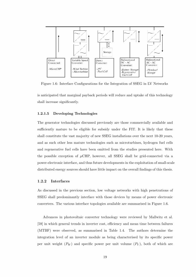
Figure 1.6: Interface Configurations for the Integration of SSEG in LV Networks

is anticipated that marginal payback periods will reduce and uptake of this technology

shall increase significantly.

1.2.1.5 Developing Technologies

The generator technologies discussed previously are those commercially available and

sufficiently mature to be eligible for subsidy under the FIT. It is likely that these

shall constitute the vast majority of new SSEG installations over the next 10-20 years,

and as such other less mature technologies such as microturbines, hydrogen fuel cells

and regenerative fuel cells have been omitted from the studies presented here. With

the possible exception of µCHP, however, all SSEG shall be grid-connected via a

power-electronic interface, and thus future developments in the exploitation of small-scale

distributed energy sources should have little impact on the overall findings of this thesis.

1.2.2 Interfaces

As discussed in the previous section, low voltage networks with high penetrations of

SSEG shall predominantly interface with those devices by means of power electronic

converters. The various interface topologies available are summarised in Figure 1.6.

Advances in photovoltaic converter technology were reviewed by Mallwitz et al.

[59] in which general trends in inverter cost, efficiency and mean time between failures

(MTBF) were observed, as summarised in Table 1.4. The authors determine the

integration level of an inverter module as being characterised by its specific power

per unit weight (PW ) and specific power per unit volume (PV ), both of which are

19

negatively affected by increases in device complexity and protection class as increased

power handling capabilities are sought. A range of future developments are identified,

including new semiconductor materials based on SiC and GaN to reduce switching

losses, and increased switching frequencies requiring advanced magnetic materials and

components.

Table 1.4: Trends in Solar Inverter Development [59]

Year 1990 2009 2015

Cost £0.9/W £0.3/W £0.2/WEfficiency 90% 96 - 98% 97 - 99%MTBF 0.1M hrs 0.5M hrs 1M hrs

A similar review of converter topologies for small wind applications can be found in

the paper by Baroudi et al. [60], in which the main PMSG diode rectifier - converter

configurations are compared in terms of cost, complexity and control requirements. It

is found that the combination of a simple diode bridge rectifier, dc boost circuit and

hard-switching inverter typical of commercially available converter modules offers a

good mix of low cost and flexibility, though controllability is somewhat limited by the

passive nature of the rectifier stage.

Finally, the paper by Emhemed et al. [61] gives an overview of the performance

of direct-connected single phase induction generators typical of those used in µCHP

systems. Particular attention is paid to the transient stability of low-rated machines in

response to faults on the 400V and 11kV networks. It is found that for LV networks

with high penetrations of small induction machines, fault ride-through is of concern

due to the lack of speed control in grid-connected mode. It is noted that the use of

static VAR compensation to mitigate voltage dips on such a network shall improve the

stability margin of all adjacent machines, and recommends an aggregated approach to

such remedial measures based on considerations of cost and complexity.

1.2.3 Impact on Grid Operation

Regardless of the particular technologies employed, mass-integration of SSEG into

low-voltage power networks will increasingly impact upon the operations of the DNOs.

A number of authors have identified symptoms associated with increasing SSEG penetration

20

levels [25,62–66], and impact studies of the following are numerous in the literature:

• Network power flows.

• Voltage regulation, rise and unbalance.

• Distribution system losses.

• System fault levels.

• Harmonic and DC current injection.

• Reliability and outage probability.

The above effects may be variously beneficial or detrimental to operation of the

distribution networks, dependent primarily on the percentage penetration of SSEG

relative to feeder capacity. Studies of these phenomena are reviewed in the following

subsection.

1.2.3.1 Power Flows

In the paper by Thomson and Infield [67], the authors present a developed load-flow

analysis tool for the evaluation of time-varying power flows on LV networks with high

penetrations of grid-connected PV and µCHP systems. This tool is used to simulate

mean voltage and network losses on a real 11/0.4kV network in Leicester, in order to

determine feasible penetration levels of SSEG according to the 10-minute mean voltage

range allowance BS EN 50160 [68]. It is found that a combined penetration of PV (28%

of customers) and µCHP (23% of customers) marginally satisfies the requirements of BS

EN 50160 without the need for network alterations. It is noted that increasing capacity

beyond these limits by adjustment of LV transformer taps is not necessarily the best

course of action as minimum winter voltages remain largely unchanged, particularly in

the case of high PV penetration. A system of distributed automatic voltage control

(DAVC), in which SSEG inverter interfaces supply or consume reactive power as a

means of network voltage improvement, is proposed.

A feature of high SSEG penetration is a reduction in mean net feeder demand.

Due to source variability, however, predictability of instantaneous power flows on the

network will be reduced in relation to a more traditional demand model. In cases where

peak generation is coincident with times of minimum demand, power flows across the

21

Figure 1.7: Generic UK LV Distribution Network as Presented in [23,25,33]

11/0.4kV and primary transformers may be reversed. This aspect has been investigated

by Cipcigan and Taylor [23] with regard to the penetration of small wind turbines, using

a PSCAD model of the UK generic LV network illustrated in Figure 1.7.

The authors found that with a minimum average customer demand of 0.16kW and

accounting for diversity of generator output, reverse power flow across the 11/0.4kV

transformer occurred at a penetration threshold of only 10% of primary transformer

capacity. Reverse flows across the primary transformer itself were observed at penetration

in excess of 82.5%, with typical transformer power handling capability being exceeded

for a 100% penetration scenario, in which a 1.1kWe source is installed in the home of

each individual customer.

Trichakis et al. [25] also make use of the UK generic LV network to evaluate the

maximum allowable penetration of SSEG on a single 0.5kVA LV feeder, supplying an

average 384 customers. Based solely on cable and transformer thermal limits, and

an even radial distribution of generator infeed, a maximum allowable penetration of

610kWe was determined for generators operating at unity power factor. This allowance

is reduced to 585 and 550kWe for 0.95 leading and 0.95 lagging power factors respectively,

reflecting the narrow operating range of a typical grid inverter.

Conti et al. [69] investigate allowable penetration levels of SSEG in the context

of transformer and cable thermal constraints, and attempt to evaluate the maximum

22

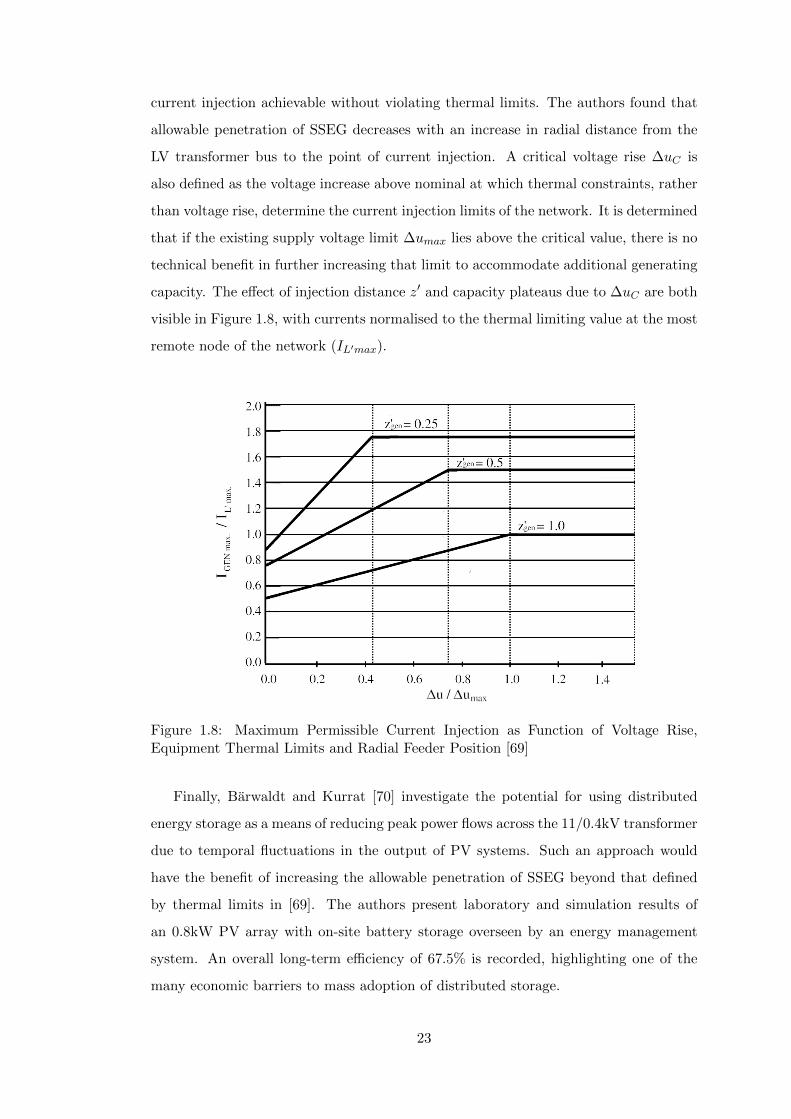
current injection achievable without violating thermal limits. The authors found that

allowable penetration of SSEG decreases with an increase in radial distance from the

LV transformer bus to the point of current injection. A critical voltage rise ∆uC is

also defined as the voltage increase above nominal at which thermal constraints, rather

than voltage rise, determine the current injection limits of the network. It is determined

that if the existing supply voltage limit ∆umax lies above the critical value, there is no

technical benefit in further increasing that limit to accommodate additional generating

capacity. The effect of injection distance z′ and capacity plateaus due to ∆uC are both

visible in Figure 1.8, with currents normalised to the thermal limiting value at the most

remote node of the network (IL′max).

Figure 1.8: Maximum Permissible Current Injection as Function of Voltage Rise,Equipment Thermal Limits and Radial Feeder Position [69]

Finally, Barwaldt and Kurrat [70] investigate the potential for using distributed

energy storage as a means of reducing peak power flows across the 11/0.4kV transformer

due to temporal fluctuations in the output of PV systems. Such an approach would

have the benefit of increasing the allowable penetration of SSEG beyond that defined

by thermal limits in [69]. The authors present laboratory and simulation results of

an 0.8kW PV array with on-site battery storage overseen by an energy management

system. An overall long-term efficiency of 67.5% is recorded, highlighting one of the

many economic barriers to mass adoption of distributed storage.

23

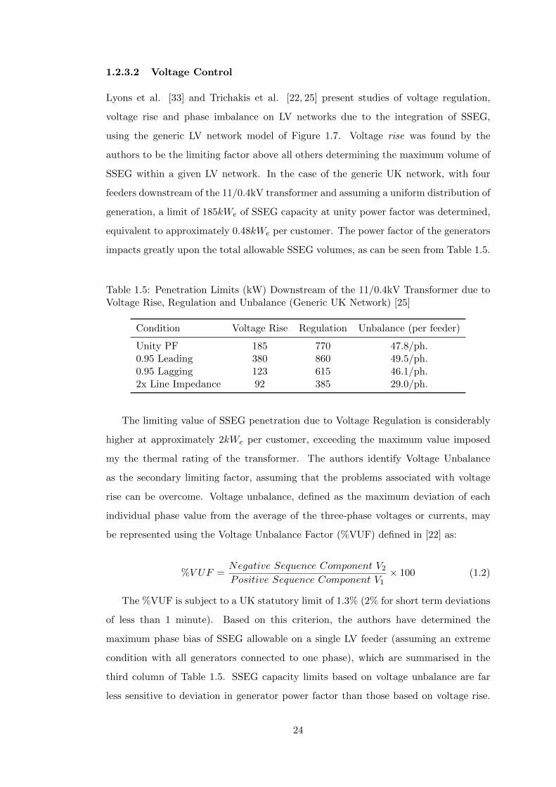
1.2.3.2 Voltage Control

Lyons et al. [33] and Trichakis et al. [22, 25] present studies of voltage regulation,

voltage rise and phase imbalance on LV networks due to the integration of SSEG,

using the generic LV network model of Figure 1.7. Voltage rise was found by the

authors to be the limiting factor above all others determining the maximum volume of

SSEG within a given LV network. In the case of the generic UK network, with four

feeders downstream of the 11/0.4kV transformer and assuming a uniform distribution of

generation, a limit of 185kWe of SSEG capacity at unity power factor was determined,

equivalent to approximately 0.48kWe per customer. The power factor of the generators

impacts greatly upon the total allowable SSEG volumes, as can be seen from Table 1.5.

Table 1.5: Penetration Limits (kW) Downstream of the 11/0.4kV Transformer due toVoltage Rise, Regulation and Unbalance (Generic UK Network) [25]

Condition Voltage Rise Regulation Unbalance (per feeder)

Unity PF 185 770 47.8/ph.0.95 Leading 380 860 49.5/ph.0.95 Lagging 123 615 46.1/ph.2x Line Impedance 92 385 29.0/ph.

The limiting value of SSEG penetration due to Voltage Regulation is considerably

higher at approximately 2kWe per customer, exceeding the maximum value imposed

my the thermal rating of the transformer. The authors identify Voltage Unbalance

as the secondary limiting factor, assuming that the problems associated with voltage

rise can be overcome. Voltage unbalance, defined as the maximum deviation of each

individual phase value from the average of the three-phase voltages or currents, may

be represented using the Voltage Unbalance Factor (%VUF) defined in [22] as:

%V UF =Negative Sequence Component V2

Positive Sequence Component V1× 100 (1.2)

The %VUF is subject to a UK statutory limit of 1.3% (2% for short term deviations

of less than 1 minute). Based on this criterion, the authors have determined the

maximum phase bias of SSEG allowable on a single LV feeder (assuming an extreme

condition with all generators connected to one phase), which are summarised in the

third column of Table 1.5. SSEG capacity limits based on voltage unbalance are far

less sensitive to deviation in generator power factor than those based on voltage rise.

24

Indeed, at unity power factor, the capacity limits are equivalent given that each 0.5MVA

transformer supplies four identical feeders. The effect of the cable impedance is far

greater, with a doubling of Z reducing allowable SSEG volumes by around 40%.

Chiradeja and Ramakumar [62,63], in their work on quantifying the system benefits

of distributed generation have proposed an indexing system for comparison of different

embedded generation scenarios. Three indices are defined for the evaluation of voltage

profile improvement (VPII), line-loss reduction (LLRI) and environmental impact reduction

(EIRI), with an overall benefit index (BI) calculated as a weighted sum according to

the priorities of the DNO.

The VPII is defined as the ratio of the voltage profile measure VP in cases with and

without distributed generation. VP itself is calculated using Equation (1.4), where N

is the total number of network load buses, Vi is the p.u. voltage at bus i, Si is p.u. load

at i, and ki is a weighting factor reflecting the criticality of a given load. In all cases,

ki must satisfy Equation (1.5).

V PII =V Pwith SSEG

V Pwithout SSEG(1.3)

V P =N∑i=1

ViSiki (1.4)

N∑i=1

ki = 1 (1.5)

Simulations are performed to evaluate each index, together with weighting-factor

sensitivity analyses, for a 12-bus 33kV network. Such a benefit indexing method could

conceivably be applied at low-voltage for the assessment of SSEG integration scenarios.

Another paper by Conti et al. [71] concerns the development of analytical methods

to evaluate the impact of SSEG on network voltage profiles, and thus the maximum

allowable volume of embedded generation that may be connected to a single feeder

without the need for relaxation of statutory supply voltage limits. For a single feeder of

unit length, the maximum permissible current injection at any position z′gen is presented

in Figure 1.9 for a range of normalised load distribution factors λLN .

25

Figure 1.9: Allowable SSEG Current Injection at Radial Position z′gen for DifferentLoad Distributions λLN [71]

The factor λLN is a measure of the uniformity of load distribution on the feeder. It

is the equivalent normalised radial distance from the transformer bus of a single lumped

element representation of the distributed load profile of the feeder. It is calculated using

(1.6), where z′ is the normalised radial distance and iL is the distributed load current

as a function of z′.

λLN =

∫ 10 z′ · iL(z′)dz′∫ 1

0 iL(z′)dz′(1.6)

With reference to Figure 1.10, a uniformly distributed feeder load has λLN =1

2,

while a triangularly descending load profile gives λLN =1

3. Thus, from Figure 1.9,

a feeder load bias toward the remote end of the line increases the scope for voltage

improvement, raising the headroom for generator current injection igen as z′ → 1.

Fletcher et al. [72] investigated the potential for voltage support in rural feeders

using distributed grid-tied PV. The authors noted significant voltage profile improvement

in networks with near unity load power factors, as illustrated in Figure 1.11. For

lagging power factors below 0.7, the inability of a small grid inverter to provide reactive

compensation means that only minimal gains in line capacity can be made using SSEGs.

The presence of SSEG may be beneficial in maintaining statutory voltage limits

26

Figure 1.10: Uniform and Triangular LV Feeder Load Profiles [71]

Figure 1.11: Voltage Profile Improvement and Reduced Line Capacity Usage on a RuralLV Feeder with SSEG and Near-Unity Power Factor Load [72]

during system voltage dips. Renders et al. [73] attempt to evaluate, and propose

improvements to, the system voltage dip immunity of voltage source converter based

SSEG interfaces. It is of note that generators rated below 16A per phase must disconnect

from the grid within 1 second in response to prolonged voltage dips below 90% of

nominal [5,6]. It is important that the response time of the disconnector is sufficient to

distinguish between short duration dips of the order of 1 or 2 cycles, and the prolonged

dips specified in ER G83/1. The authors note that high penetrations of SSEG with

overly sensitive voltage dip detection, rather than supporting the voltage may lead to

more severe voltage dip conditions as generating capacity is removed from the network.

27

Figure 1.12: Impact of SSEG on Networks Losses [25]

1.2.3.3 Losses

One of the potential benefits of SSEG from a network operator’s perspective, as identified

by a number of authors, is a reduction in I2R losses as transmission and distribution

capacity is freed up. As a best-case indication of loss reduction, one might assume the

output of a given SSEG or cluster of SSEGs to coincide with the time of peak demand,

thus curtailing the maximum current flows on the network. In reality, however, as with

any detailed system impact study, the variability of PV and CHP and locally stochastic

output profile of wind generation must all be accounted for.

In addition to their work on voltage rise, reverse power flow and thermal limit

considerations, Trichakis et al. [25] investigate the impact of SSEG on network losses

downstream of an 11/0.4kV transformer using the generic UK distribution network

model (Figure 1.7). Instantaneous network losses are evaluated downstream of the 11kV

bus under average customer maximum load (1.3kWe) and minimum load (0.16kWe)

conditions, for a range of SSEG infeed volumes. The observed characteristics are

illustrated in Figure 1.12.

As one might expect, losses on the network are minimised in instances where local

generation matches local demand. Due to the variability of both load and source,

however, optimal loss minimisation scenarios will rarely occur in practice without

28

(a) Suburban (b) Rural

Figure 1.13: Annual Network Loss Reduction with Increasing SSEG Penetration [66]

additional load control. Figure 1.12 does highlight one important consideration - the

coincidence of high SSEG availability and low local load may inadvertently lead to an

increase in network losses. There will, therefore, be an optimal SSEG penetration for

loss reduction on a given feeder loading profile. It should also be noted that both load

and generation are assumed to be uniformly distributed along the line.

While extreme operating scenarios offer an insight into network loss reduction

with SSEG, a more thorough evaluation requires the investigator to take a long-term

perspective. Such an approach might account for hourly or half-hourly load/generation

variability in order to compare cumulative energy losses over the course of a year.

Silva and Strbac [66] take a more detailed approach to the evaluation of network

losses with different penetrations of PV and µCHP. The authors’ models, based on

real distribution network topologies, account for the hourly and seasonal variability

of customer demand and SSEG output in order to evaluate losses as a percentage of

annual energy demand. Figure 1.13 illustrates the impact of each SSEG technology on

the losses in suburban and rural networks with different substation densities.

Percentage penetration here is defined as the proportion of customers with either a

1.1kWe rated µCHP or 1kW PV installed. It can be seen that despite reverse power

flow losses at peak generation with minimum load as predicted in [25], the net annual

energy loss is consistently reduced by an increase in SSEG penetration.

Finally, Chiradeja and Ramakumar [63, 74, 75] in their work on benefit indexing

29

of SSEG in LV networks have proposed a Line-Loss Reduction Index (LLRI) for the

comparison of different penetration scenarios. In a similar manner to their voltage-profile

improvement index, the LLRI is determined by comparison of the total line losses (LL)

before and after addition of SSEG to an LV feeder as given in Equation (1.7).

LLRI =LLwith SSEG

LLwithout SSEG(1.7)

LL =

M∑i=1

I2i RiDi (1.8)

The quantity LL is the sum of losses in each section of cable or overhead line, as

calculated in (1.8), where Ii is the current flowing in the ith line, Ri is the resistance

per unit length of conductor i, Di is the length of the ith conductor and M is the

total number of constituent line segments. Using this definition, the LLRI is in fact

the per-unit power loss as related to the 11/0.4kV transformer rating, which can be

straightforwardly calculated if all power flows into and out of the network are known.

Otherwise, current probes must be inserted into, and Ri evaluated for, each line

segment. The authors demonstrate the use of the LLRI by application to a 33kV meshed

network with distributed generation, but it can similarly be applied at Low-Voltage.

1.2.3.4 Additional Considerations

Other technical considerations relating to the connection of SSEG to utility networks are

summarised by O’Gorman and Redfern [65]. In addition to the impact studies already

discussed, the authors are primarily concerned with the behaviour of LV networks under

fault conditions, where a portion of fault current is supplied by embedded generation.

It is noted that fault current contribution from a remote end of a feeder may result in

maloperation or delayed operation of protection systems, and that low inertia sources

with power electronic interfaces can easily lose synchronism during a fault.

High speed disconnection of SSEGs under fault conditions as specified in ER G83/1

[5] is therefore required, but this has the detrimental effect that unfaulted generators

are unavailable during the post-fault system recovery. The improvement of SSEG fault

ride-through capability is of course key to the successful development of islandable

microgrid system models, but such scenarios are beyond the scope of this thesis. We

30

consider all SSEG in later chapters to act only as a switched negative load, as currently

treated by all UK DNOs.

Schwaegerl et al. [76] present an indexing system to evaluate the impact of distributed

generation on LV network reliability. Reliability indices based on a number of measures

are developed, as summarised in Table 1.6.

Table 1.6: LV Network Reliability Indices as per [76]

Index Unit

Fi Supply Interruption Frequency per-annumDi Mean Duration of Interruption hrs or minsQi Annual Unavailability mins/yrPi Cumulative Interrupted Power MVA/yrEi Cumulative Energy Not Supplied MVAh/yrCi Cumulative Interruption Cost £/yr

By application of this indexing system to a representative residential 20/0.4kV

distribution system in Germany, it is demonstrated that a minimum reliability cost

exists at the equivalence point of interruption and investment costs. Though DNO

operating costs have little bearing on this work, a similar evaluation system might be

employed to determine the likelihood of encountering a given SSEG network penetration

scenario. The associated overall reliability index can also be used as an indicator of the

number of SSEG disconnection events that may be encountered in any one year.

Finally, a number of impact studies relating to power quality in LV netwotks have

been performed. Good examples include work by Bhowmik et al. [77] on allowable

SSEG penetration in accordance with supply harmonic limits, and the work of Gertmar

et al. [78] on DC current injection with non-isolated grid inverters.

Supply harmonic limits provide an additional criterion for determining SSEG capacity

scenarios, but are assumed to be less severe than the voltage rise limits presented in [25].

DC injection meanwhile has been largely eliminated from the studies presented in later

chapters by use of isolating toroidal step-up transformers between the power electronics

and output filter stage as in Figure 1.14 (typical of manufacturers’ single phase inverter

designs), but transformer-less configurations could be included if required.

31

Figure 1.14: Typical PV Grid Inverter Configuration [79]

1.3 Transients in Low-Voltage Systems

As noted earlier in this chapter, the treatment of switching transients arising within

LV networks as a direct result of SSEG integration has received little or no attention

in the literature to date. There are, however, a number of more general transient

measurement, surge propagation and power quality assessments which may be used as

a benchmark for results comparison.

1.3.1 Transient Measurement Studies

Two classic measurement studies of short duration transients in LV networks are of note.

Bull and Nethercot [80] present results of a project that gathered some 36,000 event

records over a period of approximately three months, at 19 locations in and around the

Electrical Research Association (now ERA Technology) headquarters at Leatherhead

in Surrey. Measurement locations were split among domestic premises, small industrial

supplies and local Area Board substations. In a similar fashion, Goedbloed [81] presents

an analysis of 28,000 transients logged at 40 domestic, business and industrial locations

in Eindhoven, the Netherlands, collected over a total of 3,400 measurement hours.

At the service cable entries of domestic premises, both papers report a high incidence

of transient activity in the magnitude range 50-100V, with a roughly ten-fold decrease

in incidence frequency for each doubling of the magnitude. Incidence rates presented

in both papers are summarised in Figure 1.15.

Neither author has reported measured transient voltage peaks in excess of 500V

(1.5pu) at the domestic customer supply point. This contrasts sharply with business

and industrial customers who may experience transient voltages in excess of 1000V. To

32

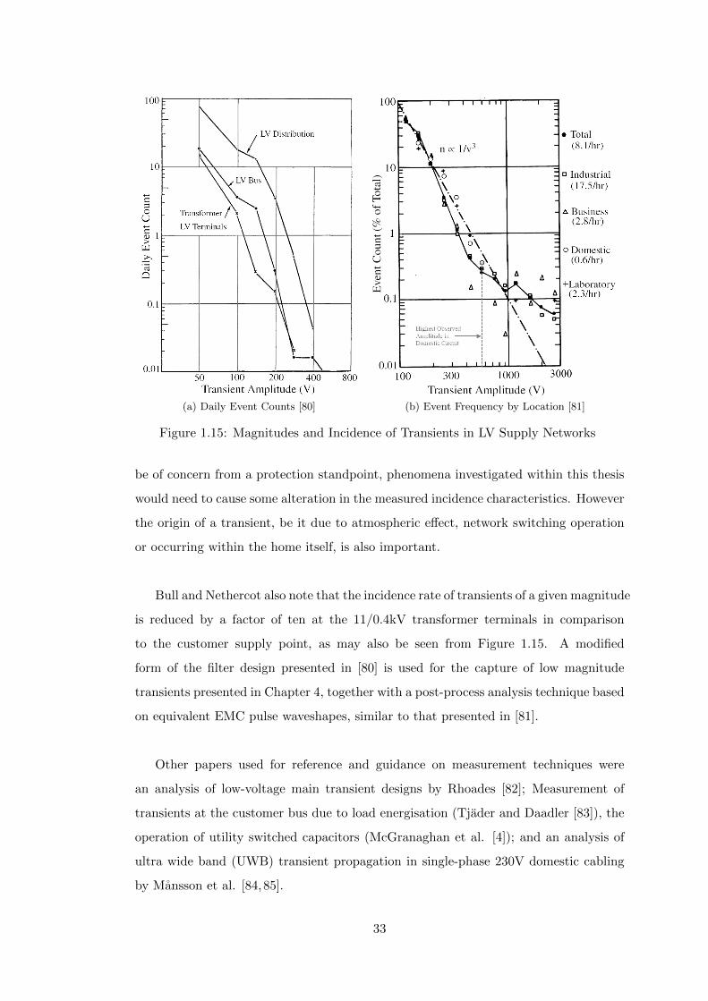
(a) Daily Event Counts [80] (b) Event Frequency by Location [81]

Figure 1.15: Magnitudes and Incidence of Transients in LV Supply Networks

be of concern from a protection standpoint, phenomena investigated within this thesis

would need to cause some alteration in the measured incidence characteristics. However

the origin of a transient, be it due to atmospheric effect, network switching operation

or occurring within the home itself, is also important.

Bull and Nethercot also note that the incidence rate of transients of a given magnitude

is reduced by a factor of ten at the 11/0.4kV transformer terminals in comparison

to the customer supply point, as may also be seen from Figure 1.15. A modified

form of the filter design presented in [80] is used for the capture of low magnitude

transients presented in Chapter 4, together with a post-process analysis technique based

on equivalent EMC pulse waveshapes, similar to that presented in [81].

Other papers used for reference and guidance on measurement techniques were

an analysis of low-voltage main transient designs by Rhoades [82]; Measurement of

transients at the customer bus due to load energisation (Tjader and Daadler [83]), the

operation of utility switched capacitors (McGranaghan et al. [4]); and an analysis of

ultra wide band (UWB) transient propagation in single-phase 230V domestic cabling

by Mansson et al. [84,85].

33

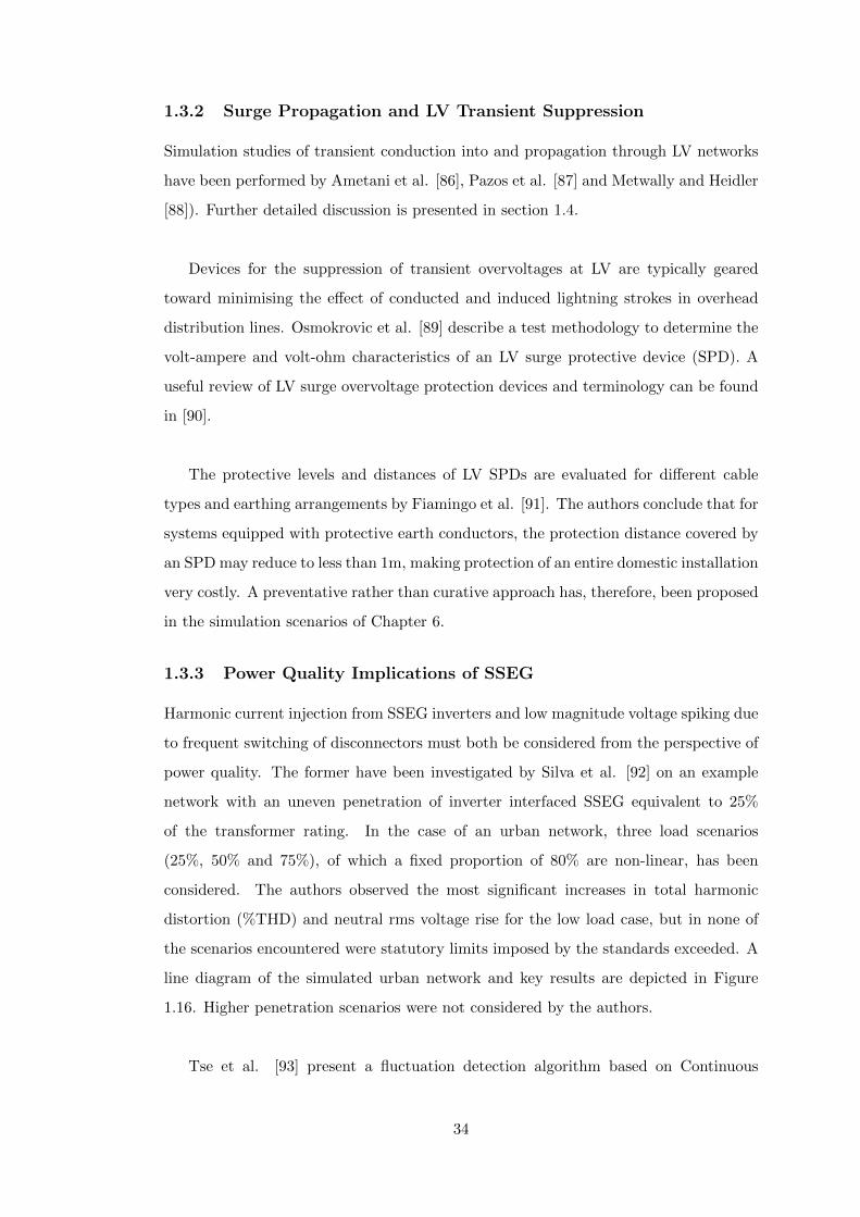
1.3.2 Surge Propagation and LV Transient Suppression

Simulation studies of transient conduction into and propagation through LV networks

have been performed by Ametani et al. [86], Pazos et al. [87] and Metwally and Heidler

[88]). Further detailed discussion is presented in section 1.4.

Devices for the suppression of transient overvoltages at LV are typically geared

toward minimising the effect of conducted and induced lightning strokes in overhead

distribution lines. Osmokrovic et al. [89] describe a test methodology to determine the

volt-ampere and volt-ohm characteristics of an LV surge protective device (SPD). A

useful review of LV surge overvoltage protection devices and terminology can be found

in [90].

The protective levels and distances of LV SPDs are evaluated for different cable

types and earthing arrangements by Fiamingo et al. [91]. The authors conclude that for

systems equipped with protective earth conductors, the protection distance covered by

an SPD may reduce to less than 1m, making protection of an entire domestic installation

very costly. A preventative rather than curative approach has, therefore, been proposed

in the simulation scenarios of Chapter 6.

1.3.3 Power Quality Implications of SSEG

Harmonic current injection from SSEG inverters and low magnitude voltage spiking due

to frequent switching of disconnectors must both be considered from the perspective of

power quality. The former have been investigated by Silva et al. [92] on an example

network with an uneven penetration of inverter interfaced SSEG equivalent to 25%

of the transformer rating. In the case of an urban network, three load scenarios

(25%, 50% and 75%), of which a fixed proportion of 80% are non-linear, has been

considered. The authors observed the most significant increases in total harmonic

distortion (%THD) and neutral rms voltage rise for the low load case, but in none of

the scenarios encountered were statutory limits imposed by the standards exceeded. A

line diagram of the simulated urban network and key results are depicted in Figure

1.16. Higher penetration scenarios were not considered by the authors.

Tse et al. [93] present a fluctuation detection algorithm based on Continuous

34

Figure 1.16: Effect of Inverter Based SSEG on %THD and Neutral Voltage Rise in theSimulated Network of [92]

Wavelet Transforms that, in addition to evaluating the harmonic content in a given

voltage waveform, is capable of determining the magnitude and frequency of a single

superimposed oscillatory transient. This method may be applied to simultaneous

power quality and transient analysis without the requirement for separate measurement

systems.

Finally, Pezos and Navarro [94] discuss field experience of power frequency overvoltages

in networks with wide scale adoption of PV systems. The overvoltages reported occur

in the time window between grid isolation of one or more inverters due to operation of

upstream circuit breakers, and the subsequent disconnection of the sources in response

to their local Loss of Mains (LoM) protection, as depicted in Figure 1.17 for a 25kWe

three phase device. Peak phase-neutral overvoltages in excess of 3.5pu have been

measured by the authors, and damage to revenue meters and other low voltage equipment

attributed to these phenomena.

1.4 Time-Domain LV Network Simulation

The final topic of this review concerns the application of digital simulation to the

solution of low-voltage transient problems, with particular reference to the modelling

of LV cables and overhead lines, distribution transformers, switches and sources.

35

Figure 1.17: Temporary Overvoltages on Upstream Isolation of PV Inverter (25kW,3φ)[94]

1.4.1 General

The primary simulation software employed in this work is a widely used royalty-free

distribution of Bonneville Power Administration’s Electromagnetic Transients Program

(EMTP). The Alternative Transient Program (EMTP-ATP), which was developed

following attempts to commercialise the previously public domain EMTP in the early

1980s [95], is together with a number of pre/post-processing tools distributed free of

charge for academic and non-commercial use under authority of the European EMTP

User Group (EEUG).

The basic time-domain digital solution method of the EMTP-ATP is based on

the algorithm presented in the 1969 paper by Dommel [96]. Many additional tools

have since been incorporated in order to expand software capability. These include

frequency dependent travelling wave line models (J. Marti, Noda . . . ) [97,98], nonlinear

components for representing varistor characteristics and transformer core saturation

[99] and supplementary tools for including and analysing control systems [100].

Specifics of the literature relating to formulation of network components and their

application in time domain simulation are discussed in the succeeding sub-sections.

General guidance on simulation component parameter estimation is given by the series

of papers by Martinez et al. [101–107], which have been used extensively in the

construction of the network models presented in Chapters 5 and 6.

36

1.4.2 Cable and Line Modelling

Many of the considerations facing the researcher studying travelling wave propagation

in low-voltage networks apply equally to the field of power-line communication (PLC).

Existing research in the modelling of PLC systems is of great use as an indicator of good

quality line and cable modelling at 11kV and 230/400V. An introductory comparison

of the different line/cable models and their characteristics is provided by Hevia [108],

ranging from the simplest lumped element equivalent PI model to the more advanced

modal and phase domain frequency dependent models of Martı and Noda respectively.

It is noted that the PI approximation, used extensively in early incarnations of the

developed network models, is far from the best choice of line representation whenever

accurate broad-band frequency response is required. This is due (a) to the fact that the

model components are evaluated at a single frequency, with degradations in accuracy

appearing with deviation from the specified solver frequency; (b) the lumped approximation

may result in spurious damped oscillation in the results which do not appear in practice;

and (c) the cascaded PI lumped approximation approach results in a network model

with many more solver nodes than there are physical system nodes, imposing limits on

the complexity and efficiency of the final simulation [108].

The solution is to employ a frequency-dependent line model, defined by its characteristic

admittance and propagation ‘constant’ which themselves are rational functions of frequency.

Options are primarily limited to the indirect modal domain model of J. Martı, and the

direct phase domain model of T. Noda, the benefits and drawbacks of each model being

discussed in Chapter 2.

The paper by Tran-Anh et al. [109] discusses the use of a J. Martı frequency

dependent transmission line for modelling medium and low voltage cabling for PLC

applications. The MV cable model developed uses three single phase sheathed cables

in a triangular arrangement, like that in Figure 1.18; a geometry that is simple to

implement in the Line and Cable Constants (LCC)routine, but ignores any outer

structure such as bedding, wire screens and external insulation. The authors accordingly

claim reasonable results with this method.

37

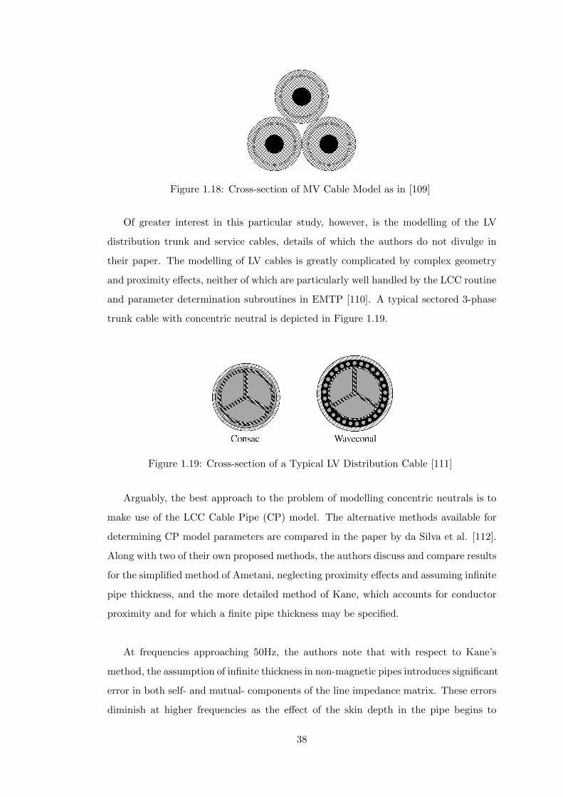
Figure 1.18: Cross-section of MV Cable Model as in [109]

Of greater interest in this particular study, however, is the modelling of the LV

distribution trunk and service cables, details of which the authors do not divulge in

their paper. The modelling of LV cables is greatly complicated by complex geometry

and proximity effects, neither of which are particularly well handled by the LCC routine

and parameter determination subroutines in EMTP [110]. A typical sectored 3-phase

trunk cable with concentric neutral is depicted in Figure 1.19.

Figure 1.19: Cross-section of a Typical LV Distribution Cable [111]

Arguably, the best approach to the problem of modelling concentric neutrals is to

make use of the LCC Cable Pipe (CP) model. The alternative methods available for

determining CP model parameters are compared in the paper by da Silva et al. [112].

Along with two of their own proposed methods, the authors discuss and compare results

for the simplified method of Ametani, neglecting proximity effects and assuming infinite

pipe thickness, and the more detailed method of Kane, which accounts for conductor

proximity and for which a finite pipe thickness may be specified.

At frequencies approaching 50Hz, the authors note that with respect to Kane’s

method, the assumption of infinite thickness in non-magnetic pipes introduces significant

error in both self- and mutual- components of the line impedance matrix. These errors

diminish at higher frequencies as the effect of the skin depth in the pipe begins to

38

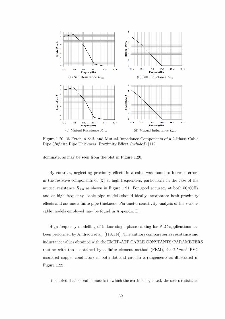
(a) Self Resistance Rnn (b) Self Inductance Lnn

(c) Mutual Resistance Rnm (d) Mutual Inductance Lnm

Figure 1.20: % Error in Self- and Mutual-Impedance Components of a 2-Phase CablePipe (Infinite Pipe Thickness, Proximity Effect Included) [112]

dominate, as may be seen from the plot in Figure 1.20.

By contrast, neglecting proximity effects in a cable was found to increase errors

in the resistive components of [Z] at high frequencies, particularly in the case of the

mutual resistance Rnm as shown in Figure 1.21. For good accuracy at both 50/60Hz

and at high frequency, cable pipe models should ideally incorporate both proximity

effects and assume a finite pipe thickness. Parameter sensitivity analysis of the various

cable models employed may be found in Appendix D.

High-frequency modelling of indoor single-phase cabling for PLC applications has

been performed by Andreou et al. [113,114]. The authors compare series resistance and

inductance values obtained with the EMTP-ATP CABLE CONSTANTS/PARAMETERS

routine with those obtained by a finite element method (FEM), for 2.5mm2 PVC

insulated copper conductors in both flat and circular arrangements as illustrated in

Figure 1.22.

It is noted that for cable models in which the earth is neglected, the series resistance

39

(a) Self Resistance Rnn (b) Self Inductance Lnn

(c) Mutual Resistance Rnm (d) Mutual Inductance Lnm

Figure 1.21: % Error in Self- and Mutual-Impedance Components of a 2-Phase CablePipe (Finite Pipe Thickness, Proximity Effect Ignored) [112]

(R11) calculated by the EMTP and FEM methods agree to within a margin of 5% over

the frequency range 50Hz to 1MHz. The self inductance (L11), however, is subject

to a fixed error of approximately 25%. If the earth is not neglected, the error in L11

at 50Hz remains large (approximately 20%), but reduces to below 5% at frequencies

above 10kHz. Of concern is the significant error introduced in the calculation of R11

over the range 0.5-500kHz, peaking at 34% at approximately 10kHz. The authors

suggest marginal conformity to assumptions of Carson’s equation/correction terms as

the source of observed errors.

By contrast, the modelling of for rural overhead cables is relatively straightforward

due to the simple geometry of the problem. Detailed studies in EMTP of LV and MV

overhead distribution lines may be found in [115] and [116] respectively, the latter being

used to determine the attenuation of high frequency signals for different customer load

types.

40

Figure 1.22: Illustrative Domestic Cable Cross-sections Used in [113,114]

(a) 700VA Inverter Transformer (b) Equivalent Circuit

Figure 1.23: Toroidal Transformer Representation for Fast-Transient Study [104,120]

1.4.3 Transformers

Modelling of the LV distribution transformer for fast-front overvoltage studies has been

performed by Mikropoulos et al. [117]. The most common transformer configuration

encountered in this work however is the single-phase toroidal transformer, common to

the vast majority of converter interfaces. Models of such transformer configurations are

non-existent in the literature. High frequency components of the transformer required

manual derivation from laboratory test results by reference to [104,118,119].

The final iteration of the toroidal transformer model consists of a linearised magnetic

circuit with lumped capacitances to represent primary, secondary and inter-winding

stray effects, as shown in figure 1.23. Detailed discussion of the transformer models

and other network components can be found in Chapter 5.

41

(a) Typical Protection Relays (b) Equivalent Circuit

Figure 1.24: Representation of Inverter Interface Relays in EMTP Simulation [121,123]

1.4.4 Relays and Circuit Breakers

As switching transient analyses shall constitute the vast majority of computational

studies in this work, the correct modelling of low-voltage circuit breakers is of importance.

Switching models vary widely in scope and complexity, from the most simple ideal

open/short circuit [121] through to elaborate nonlinear representations of switching

arc dynamics for the analysis of re-strike phenomena [122]. Due to the high recovery

voltage withstand capability of typical 230V electromechanical relays, coupled with

need to represent tens or even hundreds of independently specified switching operations,

a simplistic approach was adopted for the of modelling these devices.

Relays have been here modelled as ideal switches in parallel with an open position

contact capacitance obtained from the relevant relay datasheet. Series impedance in

the closed position may be ignored as it is negligible in comparison with that of both

the incoming circuit and the device being isolated. An example of this representation

is given in Figure 1.24. Further detail may be found in in Chapter 2

1.4.5 Pertinent Studies

Electromagnetic transient phenomena arising due to small-scale embedded generators

connecting to and disconnecting from low voltage distribution networks have not, to

the author’s knowledge, been the prime focus of any existing research to date. The

somewhat broad nature of this review is testament to this assertion.

42

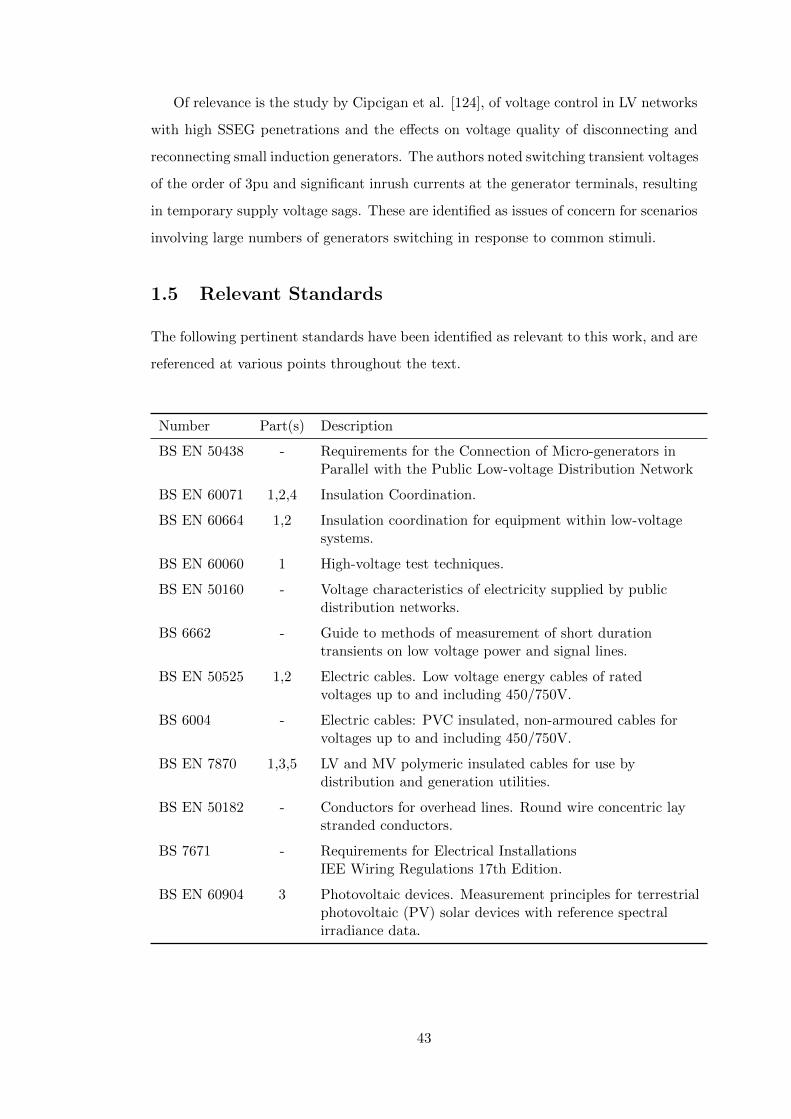
Of relevance is the study by Cipcigan et al. [124], of voltage control in LV networks

with high SSEG penetrations and the effects on voltage quality of disconnecting and

reconnecting small induction generators. The authors noted switching transient voltages

of the order of 3pu and significant inrush currents at the generator terminals, resulting

in temporary supply voltage sags. These are identified as issues of concern for scenarios

involving large numbers of generators switching in response to common stimuli.

1.5 Relevant Standards

The following pertinent standards have been identified as relevant to this work, and are

referenced at various points throughout the text.

Number Part(s) Description

BS EN 50438 - Requirements for the Connection of Micro-generators inParallel with the Public Low-voltage Distribution Network

BS EN 60071 1,2,4 Insulation Coordination.

BS EN 60664 1,2 Insulation coordination for equipment within low-voltagesystems.

BS EN 60060 1 High-voltage test techniques.

BS EN 50160 - Voltage characteristics of electricity supplied by publicdistribution networks.

BS 6662 - Guide to methods of measurement of short durationtransients on low voltage power and signal lines.

BS EN 50525 1,2 Electric cables. Low voltage energy cables of ratedvoltages up to and including 450/750V.

BS 6004 - Electric cables: PVC insulated, non-armoured cables forvoltages up to and including 450/750V.

BS EN 7870 1,3,5 LV and MV polymeric insulated cables for use bydistribution and generation utilities.

BS EN 50182 - Conductors for overhead lines. Round wire concentric laystranded conductors.

BS 7671 - Requirements for Electrical InstallationsIEE Wiring Regulations 17th Edition.

BS EN 60904 3 Photovoltaic devices. Measurement principles for terrestrialphotovoltaic (PV) solar devices with reference spectralirradiance data.

43

1.6 Chapter Summary

In this chapter, a review of literature on the topics of embedded generation technology,

low-voltage transient measurements and time-domain circuit simulation techniques

has been presented. Given the relative novelty of electromagnetic transient studies

at low voltages, particularly those relating to embedded generation, the number of

immediately relevant research papers was found to be few. Accordingly, a fairly broad

range of review topics has been included, covering published papers, standards and

guidelines in the aforementioned areas. In the next chapter, suitability of electromagnetic

transient simulation tools for low-voltage application is assessed.

44

Chapter 2

Time-Domain SimulationSuitable for Low-Voltage Systems

In this chapter, aspects of electromagnetic transient simulation pertaining to the

modelling of low-voltage networks are discussed. Consideration is given to the

modelling of individual network components and appropriate simulation setup

criteria, with the ultimate goal of developing representative LV network, embedded

source and load models in EMTP-ATP.

2.1 Overview of Time-Domain Simulation

Simulation of electrical networks is an essential process in the design and engineering

of modern power systems. Where an existing system configuration is to be altered by

some action, by addition or removal of generation, bulk load or transmission capacity,

good simulation methods are necessary in order to predict and manage any associated

changes in performance.

Steady-state simulations are used to approximate the power flows and voltage

profiles across complex power systems under a given set of time-invariant conditions.

Iterative computational methods, such as the Gauss-Seidel and Newton-Raphson algorithms

[125], are widely employed in order to determine the power flow solution where the size

and complexity of a network prohibits an efficient method of determining an exact

analytical solution.

45

When the network configuration changes over time, or is subject to disturbance,

a power system may be considered to occupy a transient state [126], and steady-state

methods alone are no longer capable of computing the associated time-variant quantities.

Thus, time-domain analyses become necessary to determine the dynamic performance of

a large electrical network. This type of simulation constitutes a diverse range of possible

system studies, broadly categorised in terms of their duration and constituent frequency

components. These criteria in turn determine the time-step resolution necessary in

order to observe and analyse a given phenomenon:

• Load and Generation Profiling [127]; Allow minute by minute or hourly assessment

of load flow variations on a power system by computation of a sequence of

steady-state snapshots (1s < ∆t < hours).

• System Dynamic Simulations; Take account of the electromechanical and control

characteristics of generators and loads in order to assess the system stability in

response to a sudden change in configuration e.g. dynamic fault studies and

assessment of power-frequency temporary over-voltages (TOV) due to switching,

line/transformer energisation or resonance in networks with large LC components

(∆t ≈ 1ms).

• Slow-front Transient Analysis [120]; Typically associated with over-voltages arising

due to the switching of system components, e.g. line energisation, fault clearing

and the making and breaking of capacitive or inductive loads. These techniques

typically require numerical solution of the time-domain differential equations

governing the electrical network in question. (∆t ≤ 10µs).

• Fast-front Transient Analysis; Mainly concerned with the impact of lightning

strokes to and in the vicinity of electrical power lines and installations, but

also applicable to certain switching operations. Travelling wave phenomena are

important in all but the shortest line sections (∆t ≤ 100ns).

• Very-fast-front Transients; Usually observed in flashover of gas-insualted switchgear

(GIS), though similar analysis techniques have application in close proximity

(undamped) lightning studies and switching in lower voltage systems. Such

studies require knowledge of the power system response at very high frequencies

(up to 100MHz) and model components accordingly share few similarities with

their 50Hz counterparts (∆t ≤ 1ns)

46

For a fixed real time window, the computation time and memory requirement of

a simulation increase in inverse proportion to the size of the required time step ∆t.

Consequently, the extent both in time and space of a solution will be largely dictated by

the frequency components of the phenomenon of interest; any over-specification in the

simulation set-up will result in wasted computing resource. It is not uncommon to find

steady state load flow models representing entire national transmission networks, but

a sufficiently comprehensive lightning fast-front over-voltage (FFO) study might only

consider a single substation and its proximate overhead lines and cables. Very-fast-front

over-voltage (VFFO) studies may even be confined to an individual substation bus

section and remain suitably representative of real phenomena.

Such considerations will be addressed in this chapter with a view towards high

resolution time-domain simulation of low voltage networks. This will allow comprehensive

studies of electromagnetic transients in such networks to be undertaken, with particular

relevance to the impact of ubiquitous small-scale embedded generation (SSEG).

2.2 Numerical Solution of Electromagnetic Transients

Numerical integrator substitution is a method for the time-domain computation of

variables in physical systems. The method was developed in the late 1960s for application

in digital simulation of electrical networks, as a more flexible and powerful alternative

to the analogue Transient Network Analyser (TNA). It forms the basis of Dommel’s

Electromagnetic Transient Program (EMTP) [96,123], a widely used and accepted tool

for the simulation of electromagnetic phenomena in power systems.

2.2.1 The Trapezoidal Rule and Linear Circuits

For the purposes of digital simulation, continuous systems must be converted to discrete

time equivalents, either as a z-domain transfer function or a set of branch difference

equations. This is most commonly achieved using the closed first order Newton-Cotes

numerical integration method, commonly known as trapezoidal integration, and is the

method employed in the EMTP-ATP simulation package due to its simplicity, stability

and accuracy in the majority of cases [123].

The solution method works by discretising all components of a given linear network

47

to branch difference equations by numerical integration, followed by formation of the

network branch conductance matrix [G]. The circuit may then be solved for each

successive discrete time step using the nodal equation:

[G] v(t) = i(t) + Iold (2.1)

where v(t) is the vector of nodal voltages, i(t) is the vector of present external

current sources, and Iold the vector of current sources which represents the state of

system at the previous time step.

This section aims to highlight the potential pitfalls in using trapezoidal integration

methods for the solution of low-voltage circuits, namely solution accuracy and stability,

and considerations of matrix conditioning. For a general summary of trapezoidal

integration and its application to linear circuit elements, please refer to Appendix A.

2.2.1.1 Accuracy of Solution

It can be easily shown that the branch difference equation, generated by Dommel’s

method for a given arrangement of linear components, is equivalent to a first-order

approximate Taylor series expansion of the exponential function:

e−x =e−

x2

ex2

'1− x

2

1 +x

2

(2.2)

where x =∆tR

Lfor an RL branch or

∆t

RCfor an RC branch. Since the exact

circuit response is exponential in nature, this approximation results in a truncation

error dependent on the ratio of solution timestep and branch time constant. ∆t must,

therefore, be carefully chosen to account for the shortest time constants and highest

frequency components in the system. It is preferable to select a value no greater than

one third of the shortest time constant of the circuit [128] (τmin) in order that erroneous

simulated circuit behaviour be avoided.

It is possible to minimise such errors through the use of exponential functions in

the system difference equations, thereby better approximating an analytical solution.

This method is known as the Root Matching (Euler) approach, in that it exactly maps

the roots of the frequency domain equivalent admittance matrix from the s- to the

48

z-domain, eliminating the truncation error described above. For further details, see

Appendix A

2.2.1.2 Stability

For the purpose of converting a continuous system to a discrete one, the trapezoidal

integrator is equivalent to bilinear transformation. An important consequence of this

equivalence is that if the continuous time transfer function of the network being modelled

is stable, the resulting discrete system will itself be stable [123]. This is one of the

reasons that the EMTP (employing Dommel’s method) is the favoured solution method

in this work.

It must be emphasised, however, that the stability of a solution does not imply

its exactness, nor indeed vice versa. Certain circuit configurations involving minimally

damped RLC branches or short τ values are susceptible to marginal numerical stability

when the trapezoidal rule is employed in its differential form. The result is a node

voltage or branch current that oscillates about the exact solution, reversing in polarity

with each successive time step. This fictitious circuit behaviour is known as numerical

oscillation [123]. For a discussion of causes, effects and mitigation of this phenomenon,

see Appendix A

2.2.1.3 Conditioning

As a general observation on the limiting factors of the EMTP solution method, the

conditioning of the system steady-state admittance matrix [Y] and the time-domain

conductance matrix [G] must be considered. As a general rule, it is advised that the use

of extremely small branch resistances and inductances in a simulation be avoided. This

is because the formation of network the Y- and G-matrices generates very large values

which tend to obscure the behaviour of other components connected to the same node.

A similar limitation applies to very large capacitances, though values large enough to

cause ill-conditioning of the conductance matrix are unlikely to be encountered in any

practical scenario. Equations (2.3) to (2.5) summarise the admittance and effective

conductance components in the EMTP solution.

49

for a Resistor, we have Y =1

R, G =

1

R(2.3)

for an Inductor, we get Y =1

ωL, Geff =

∆t

2L(2.4)

and in the case of a Capacitor Y = ωC, Geff =2C

∆t(2.5)

Conversely, very large resistances and inductances or very small capacitances will

produce very small Y- and G-matrix components, effectively removing them from the

solution altogether. This is of far lesser concern as it has little or no effect on the final

results. Ill-conditioning of the network conductance matrix is a prime cause of solution

inaccuracies and should be actively avoided in all simulations [110,123].

Due to small circuit time constants and line travel times, electromagnetic transient

simulation of Low-Voltage networks will generally require very short simulation time

steps. This requirement will tend to counteract the conditioning problems caused by

small inductances as the effective conductance is proportional to ∆t. The effective

conductance of a capacitive branch, however, is inversely proportional to ∆t, so a

requirement for high resolution will effectively reduce the threshold defining a very large

capacitance. It is still unlikely that sufficiently large values of C will be encountered,

but conditioning errors may be ruled out if consistent results can be demonstrated for

a range of simulation step sizes.

2.2.2 Non-linear Components

A brief general analysis of non-linear component representation in EMTP is given here

in order to highlight some important features.

The solution methods discussed in section A.1 are ideally suited to the accurate

analysis of linear circuits in the time domain. The modelling of non-linear components,

such as metal oxide varistors (MOV) and saturable transformer cores, can by contrast

be very accurately modelled by the use of non-linear techniques. Unfortunately, it is

not possible to combine these techniques in solving a single circuit consisting of both

linear and non-linear components, and thus a single technique must be made to work

50

for all components. Non-linear circuit analysis techniques involving representations

of all component characteristics by continuous analytical functions can be employed,

but present a wasteful computational burden when only a small proportion of circuit

components are non-linear. Far more efficient linear methods are, therefore, modified

in order to approximate a particular device performance [110].

2.2.2.1 Non-linear Inductors

Piecewise linear inductances, defined by a given flux-current characteristic, are implemented

in the EMTP using the ”switched” component representation shown in Figure 2.1. For

values of λ below λsat, the switch remains open, but closes once λsat is exceeded. The

result is the two-slope characteristic presented.

Figure 2.1: Two-slope Non-linear Inductor Representation

In reality, no switch exists in the circuit, and the branch inductance value is simply

changed directly within the conductance matrix [G] at the first time step following

the knee-point crossing. This transition is essentially analogous to a discontinuity in

the inductor current, and as such presents similar potential for numerical oscillation as

discussed in the previous section. The inclusion of representative core loss resistance in

a model will generally negate this problem.

In making the transition from slope L1 to L2 in the discrete time domain, there will

always be some degree of overshoot error if the exact crossing instant occurs between

time steps. The reconfigured circuit only applies from the first time step following the

51

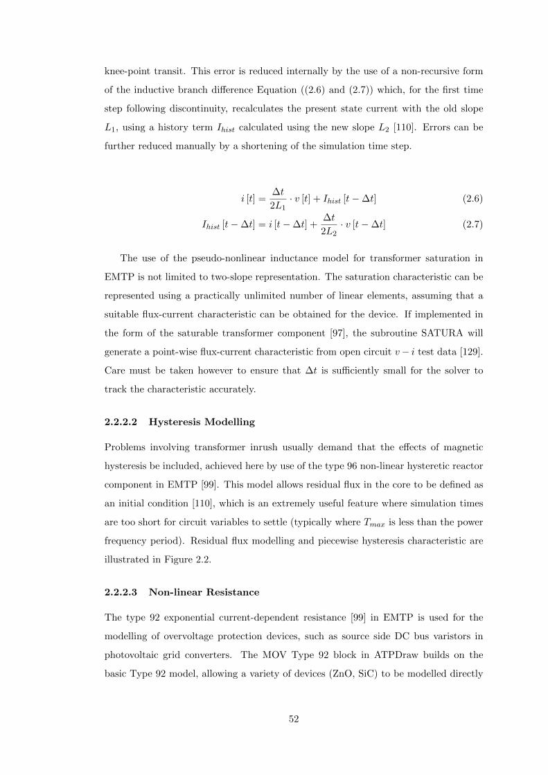
knee-point transit. This error is reduced internally by the use of a non-recursive form

of the inductive branch difference Equation ((2.6) and (2.7)) which, for the first time

step following discontinuity, recalculates the present state current with the old slope

L1, using a history term Ihist calculated using the new slope L2 [110]. Errors can be

further reduced manually by a shortening of the simulation time step.

i [t] =∆t

2L1· v [t] + Ihist [t−∆t] (2.6)

Ihist [t−∆t] = i [t−∆t] +∆t

2L2· v [t−∆t] (2.7)

The use of the pseudo-nonlinear inductance model for transformer saturation in

EMTP is not limited to two-slope representation. The saturation characteristic can be

represented using a practically unlimited number of linear elements, assuming that a

suitable flux-current characteristic can be obtained for the device. If implemented in

the form of the saturable transformer component [97], the subroutine SATURA will

generate a point-wise flux-current characteristic from open circuit v− i test data [129].

Care must be taken however to ensure that ∆t is sufficiently small for the solver to

track the characteristic accurately.

2.2.2.2 Hysteresis Modelling

Problems involving transformer inrush usually demand that the effects of magnetic

hysteresis be included, achieved here by use of the type 96 non-linear hysteretic reactor

component in EMTP [99]. This model allows residual flux in the core to be defined as

an initial condition [110], which is an extremely useful feature where simulation times

are too short for circuit variables to settle (typically where Tmax is less than the power

frequency period). Residual flux modelling and piecewise hysteresis characteristic are

illustrated in Figure 2.2.

2.2.2.3 Non-linear Resistance

The type 92 exponential current-dependent resistance [99] in EMTP is used for the

modelling of overvoltage protection devices, such as source side DC bus varistors in

photovoltaic grid converters. The MOV Type 92 block in ATPDraw builds on the

basic Type 92 model, allowing a variety of devices (ZnO, SiC) to be modelled directly

52

(a) Residual Flux (b) Piecewise Hysteresis Loop

Figure 2.2: Non-linear Hysteresis Modelling in EMTP

from the device manufacturers’ data. A least squares method is used to fit the entered

data points to the exponential formulation in (2.8) to within a defined tolerance.

i = p ·(

v

Vref

)q(2.8)

2.2.3 Transmission Lines

This section provides a general discussion of the transmission line model selection

process, and the merits and limitations of the available representations.

As a general rule, if a length of cable or overhead line to be modelled has a

travel time τ less than the solution time step ∆t, a nominal PI model with mutual

coupling of conductors, as illustrated in Figure 2.3, is considered sufficient [123]. Where

τ > ∆t, travelling wave models should always be used in order that the distributed line

parameters and propagation delays be correctly represented.

A number of travelling wave models are available, ranging in complexity from the

constant frequency lossless Bergeron model with lumped resistance approximation,

through to the frequency dependent JMarti and Noda models. If geometric and material

data for the line in question is available, it is preferred that a frequency dependent model

be used [123]. This preference becomes a requirement in cases where broad frequency

spectra are to be observed, in unbalanced problems where the zero sequence current

53

Figure 2.3: Nominal PI Line Representation

plays a significant role, or in high frequency solutions of overhead lines taking account

of eddy current induction in the earth [110].

A benefit of the use of transmission lines from the perspective of computational

requirements is that the present voltages and currents at one end of the line are

completely independent of the present states at the other. Therefore, mutual coupling in

the equivalent conductance matrix of two subsystems A and B linked by a transmission

line is eliminated, allowing the subsystems to be represented as diagonal sub-matrices

in [G] (2.9):

[G] =

[GA]

[GB]

(2.9)

The increased sparsity of the conductance matrix that arises from using transmission

line sections can greatly reduce the computational burden in simulating extensive

meshed networks. It is preferable to use a transmission line model in all cases, except

those in which it would itself impose prohibitively short ∆t requirements.

2.2.3.1 Frequency Dependent Transmission Lines

A discussion of the general aspects of frequency-dependent line representation may be

found in Appendix A.

The treatment of frequency-dependent lines and cables in the EMTP software may

be achieved by the use of a variety of models. Two such models are compared here -

one employing modal decomposition (JMarti), the other applied directly in the phase

54

domain (Noda).

2.2.3.2 Modal Domain Model (J. Martı)

This model employs a process of modal decomposition, simplifying any M-phase coupled

line into M decoupled single phase lines. Voltages and currents along the line are

determined in the phase domain by Equations (2.10) and (2.11).

[d2Vphasedx2

]=[Z ′phase

]·[Y ′phase

]· [Vphase] (2.10)[

d2Iphasedx2

]=[Y ′phase

]·[Z ′phase

]· [Iphase] (2.11)

where the products [Z ′][Y ′] and [Y ′][Z ′] are distinct except in the case where the

matrices are balanced and a lossless high-frequency approximation is assumed [110].

Modal decomposition of the phase voltage and current vectors is achieved by the use

of an appropriate transformation matrix (2.12).

[Vmode] = [TV ]−1 · [Vphase] [Imode] = [TI ]−1 · [Iphase] (2.12)

Thus, in the modal domain:

[d2Vmodedx2

]= [TV ]−1 [Z ′phase] [Y ′phase] [TV ] [Vmode] = [Λ] [Vmode] (2.13)[

d2Imodedx2

]= [TI ]

−1 [Y ′phase] [Z ′phase] [TI ] [Imode] = [Λ] [Imode] (2.14)

(2.15)

where the matrix [Λ] contains the modal eigenvalues λmode of the matrix products ZY

and YZ. The transformation matrices [TV ] and [TI ] are the eigenvector matrices, and

because [Z][Y ] 6= [Y ][Z] they are different, in contrast to their eigenvalues which are

always identical. However, only one of transformation matrices need be determined, as

they are related to each other by (2.16) [110].

[TI ] = [T tV ]−1 (2.16)

55

The modal Impedance and Admittance matrices are then given by (2.17).

[Z ′mode] = [T tI ][Z′phase][TI ] [Y ′mode] = [T tV ][Y ′phase][TV ] (2.17)

and the characteristic impedance of a given mode k is

ZC mode k =γmode kYmode k

(γmode k =

√λmode k

)(2.18)

From this point, it is a straightforward process to fit rational functions to the modal

characteristic admittances and propagation constants. These are then transformed back

into the phase domain by the use of the eigenvector matrices [TV ] and [TI ], and the

time domain equivalent of Figure A.6 generated by computing the receiving end history

term by recursive convolution.

ik hist propagation = −∫ τmax

τmin

im tot(t− u)a(u)du (2.19)

im tot = yC(t) ∗ vm(t− τmin)− im(t− τmin)

where τmin and τmax are the shortest and longest modal travel times respectively, and

yC and a are the inverse Fourier transformations of the Admittance and Propagation

matrices (see Appendix A) [110,123].

Of the frequency dependent line representations available to the EMTP user, Martı’s

model is by far the most widely used. There are, however a number of considerations

which limit its applicability to the modelling of Low-voltage networks. The primary

drawback of the modal-domain approach is that while the matrices [YC mode] and

[γmode] are themselves frequency dependent, the transformation matrices [TV ] and

[TI ] are only defined at a single frequency specified in the model set-up and thus

remain constant across the frequency range of interest [108]. This limitation impacts

the modelling of cable networks more than overhead lines, and results in errors when

applied to untransposed conductors. As such, its appropriateness for the representation

of low-voltage distribution networks in urban areas is questionable.

The fitting of the rational function to the frequency dependent modal characteristic

admittances produces an inherent instability at very low frequencies, as the functions

56

will all pass through zero if the mode shunt conductance G(ω) is omitted. Since trapped

charge investigation is not required in the studies presented in this work, this is of little

concern except in the event of dc-current injection from an embedded generator. Most

problems can be overcome by starting the function fitting from a very low frequency

(typically 10−4Hz is considered adequate [108]).

2.2.3.3 Phase Domain Model (Noda)

In order to avoid the accuracy problems caused by the mode-phase transition in the

Martı line model, it has become increasingly desirable to do away altogether with modal

transformation, and treat the fitting of frequency-dependent characteristics directly in

the phase domain [108]. Because the phase domain solution is inherently a coupled

problem, a greater number of frequency dependent components are necessary as the

off-diagonal components of the Y-matrix are non-zero. This is a minor trade-off in

favour of improved accuracy over a broad frequency range, and is more than justified

in the author’s opinion.

One of the problems associated with phase domain representation of lines is that

conversion back to the time domain by recursive convolution generates discontinuities

whenever the modal propagation times differ [98]. The solution to this problem,

as implemented in the Noda model, is to fit a rational function in the z-domain

to the frequency dependent data output by the LINE CONSTANTS and CABLE

PARAMETERS subroutines. This function fitting is performed by the external routine

ARMAFIT, which outputs auto-regressive moving average (ARMA) functions for the

line parameters of the form shown in (2.20).

G(z) =a0 + a1z

−1 + a2z−2 + · · ·+ aNz

−N

1 + b1z−1 + b2z−2 + · · · bNz−N(2.20)

When converted to the time domain, these simply produce expressions for the present

value of a variable at one terminal of the line as a sum of weighted delay terms at

the other, which is the discrete time equivalent of the recursive convolution method

required for the s-domain fitting.

57

y[t] =a0x[t] + a1x[t−∆t] + a2x[t− 2∆t] + · · ·+ aNx[t−N∆t] (2.21)

− b1y[t−∆t]− b2y[t− 2∆t]− · · · − bN [t−N∆t] (2.22)

This discrete-time function can be used directly in the EMTP simulation, making it

far more efficient than recursive convolution, and overcomes discontinuity representation

problems caused by differences in modal phase velocities. One limitation of note is that

the phase-domain line or cable model must be generated using the same time-step ∆t as

used in the simulation itself [130]. A change of solver resolution will, therefore, require

all phase domain models to be recalculated prior to simulation, but this is only a minor

inconvenience. The frequency response of a Noda model computed at a new ∆t should

always be compared with its predecessor to ensure that a correct re-fitting has taken

place.

2.3 Special Considerations in LV Networks

This section highlights a number of considerations pertaining to the modelling of

low-voltage systems in EMTP.

2.3.1 Distance and Time

Discrete time-domain simulation of electrical networks requires selection of a solution

time step and duration that is appropriate for the problem being investigated. In

general, low voltage network models will impose stringent limits on the time step

because of the short lengths of LV cables and overhead lines (compared to MV and

HV circuits), and the need to account for very fast-front transients generated close to

the customer.

The correct representation of travelling wave transmission line models requires that

the time step be no greater than half the travel time τ of the fastest propagation mode

[120]. This criterion does not, however, guarantee solution accuracy as travel times that

are a non-integer multiple of ∆t shall be subject to linear interpolation errors [110,123].

It is desirable that τmode for each propagation mode be equal to n ·∆t, where n is an

integer. This requirement is in practice very difficult to fulfil, but simulation errors

58

may be minimised by ensuring that

∆t ≤ τmode min5

(2.23)

Clearly, the reproduction of high frequency phenomena is absolutely limited by the

Nyquist sampling criterion. The maximum theoretical frequency component that can

be observed in a simulation with time-step ∆t is

fN =1

2∆tHz (2.24)

though such data would be meaningless, being indistinguishable from spurious numerical

oscillation. The inclusion of damping networks to combat numerical oscillation problems

would similarly damp the high frequency components of interest, and as such further

limits the maximum frequency reproducible at a given time step. For the steepest

expected transient voltage or current front, a minimum of 10 data points are required

in order to correctly evaluate the peak value and rate of rise [120], but a more liberal

approach has been taken here to leave sufficient headroom for the damping of numerical

problems. For a specified upper frequency bound fmax, a time step is chosen such that

∆t ≤ 1

50fmax(2.25)

For the simulation of locally generated transients, involving only a single timed

switch operation, a time-step of 1ns was chosen following multiple test executions,

to allow domestic cabling to be represented as short transmission line sections. The

modelling of multiple sources in distribution networks implies a far greater number of

solution nodes, with computational burden increasing in proportion to n2. However,

the time step requirement here can be relaxed given that minimum travel times in

distribution line and cable sections are increased, and that greater attenuation of high

frequency components with distance can be assumed. Table 2.1 summarises the impact

of selected time steps on minimum mode propagation times and maximum frequency

representation according to the criteria in (2.23) and (2.25). The minimum allowable

length of transmission line section Lmin TL is determined assuming a worst-case mode

propagation velocity equal to the speed of light in vacuo.

59

Table 2.1: Limiting Criteria as Determined by Choice of Solution Time-step

Detailed Models LV Network Models

(Domestic) Urban Rural

∆t 5ns 20ns 40nsLmin TL 3m 12m 24mfmax 4MHz 1MHz 0.5MHzTrise min 50ns 200ns 400ns

The establishment of a single ∆t for comparison studies is beneficial where phase

domain transmission line models are used, as the ARMA function can only be specified

at the exact solution time-step. In all cases, the total simulation real time window Tsim

must at least be wide enough to pick up any travelling wave reflection from the most

remote node of the model [120].

2.3.2 Conductor Geometry

The use of established overhead line and underground cable models for the representation

of low-voltage systems is not widely documented, and the assumptions made in the

development of these models must be accounted for in order to ensure that the circuits

implemented in EMTP-ATP are a true representation of real equipment. A significant

feature of LV circuits is the low X/R ratio at 50Hz, due to the small cross-sectional area

(CSA) of conductors. The attenuation constant α(ω) of a low voltage line is far higher

than that of an equivalent length of 400kV conductor and, therefore, the geographic

area of interest covered by propagating transients is very localised.

A second feature of the small CSA is that the skin depth becomes significant at

a much higher frequency than in a high voltage conductor bundle. This is illustrated

in Figure 2.4 with reference to a range of conductor stranded cross-sections. Current

is assumed to be evenly distributed among the strands of the conductors, and the

frequency-dependent resistance is normalised to the DC value. This flatter response

aids in the fitting of rational functions to the cable parameters and line constants in

the frequency domain. An estimate of the skin effect in LV 3-phase conductors at a

60

given temperature θ is given by

R(f) = RDC · (1 + ys + yp) (2.26)

with the DC resistance RDC , and skin and proximity effect factors ys and yp defined

[131] as

RDC = RO · [1 + α20(θ − 20)] (2.27)

ys =x4s

192 + 0.8x4s

(2.28)

yp =x4p

192 + 0.8x4p

(dCs

)2

·

0.312

(dCs

)2

+1.18

x4p

192 + 0.8x4p

+ 0.27

(2.29)

where x2s =

8πfksRDC

· 10−7 x2p =

8πfkpRDC

· 10−7

where RO is the dc resistance at 20C, α20 is the temperature coefficient of resistance of

the conductor material evaluated at 20C, f is the frequency in Hz, dC is the conductor

diameter in mm, and s the mean separation between conductor axes in mm. The

coefficients ks and kp are both equal to 1 for circular stranded conductors [131]. The

skin- and proximity-effect factors are multiplied by 1.5 in equivalent pipe-type cables.

An alternative method for the calculation of internal resistance is to use Kelvin

functions (modified Bessel functions) as presented in [132]. This is a more exact solution

for simple conductor geometries, and is used for the evaluation of skin effect in EMTP

line and cable models. The principal limitation of this method is that proximity effects

are unaccounted for. Resistance at high frequency is calculated by Equation (2.30),

where r is the conductor radius, ω the frequency in rad s−1 and ρ is the conductor

resistivity.

R

RDC=κ

2

Ber(κ)Bei′(κ)−Bei(κ)Ber′(κ)

Ber′2(κ) +Bei′2(κ)

(κ = r ·

√ωµ0

ρ

)(2.30)

Geometric models computed under LINE CONSTANTS and CABLE PARAMETERS

subroutines must conform to the underlying assumptions of the equations on which they

are based. All bare-conductor overhead line models used in the simulations conform

61

Figure 2.4: Skin Effect in Stranded Conductors (Circular Cross-Section) [131,132]

to the assumptions of Carson’s formula for homogeneous earth [110]. Parabolic sag is

assumed in sections shorter than 500m, and the following criteria are satisfied:

1. Conductors may be assumed to be horizontal with sag accounted for by average

height approximation, and long enough for end-effects to be ignored.

2. The air surrounding the conductors is lossless and homogeneous with permittivity

and permeability equal to that of free space.

3. The earth is also homogeneous (ε = ε0 , µ = µ0), with uniform resistivity ρ.

Electrical behaviour is that of a conductor (ωρε0 << 1), which for a critical

frequency of 4 MHz as determined in Table 2.1, places an upper limit on ρ of

4.5 kΩm. A nominal value of 100 Ωm was specified for all rural overhead lines in

this research investigation.

4. Conductor spacing ≥ 10×diameter, allowing proximity effects to be ignored.

The suitability of geometric cable models is less clear as there exists no unified

solution equivalent to Carson’s equations for OHLs [123]. Distribution cable geometries

with circular conductors and symmetric co-axial sheath construction can be modelled

quite easily using an insulated cable-pipe representation. Armoured four-conductor

cables, where a smaller neutral conductor is bundled with the three phases, are a lot

harder to represent as the individual conductors are non-circular and of varying sizes,

and the overall symmetry of the cable cross-section is lost. Indoor cabling is also difficult

to model due to the very small features involved, and the variety of environments

62

encountered makes an evaluation of a singular earth resistivity almost impossible. The

exact choice of models in this work is discussed in sections 2.4.2, 2.4.3 and 2.5.1.

2.3.3 Insulation Materials

Insulation and sheathing materials considered in the simulations were Cross-linked

Polyethylene (XLPE) for 3-phase distribution mains [133] and Extruded Poly-Vinyl

Chloride (PVC) for both indoor wiring [134] and distribution service cables [135, 136].

At present, there is no method for the inclusion of frequency-dependent dielectric

permittivity and loss factors in the insulation and sheathing of cable models. This is

of little concern as the dielectric properties of PVC and XLPE are essentially constant

over the frequency range of interest, and thus a single valued εr is considered sufficient.

2.3.4 Insulation Coordination

Insulation Coordination in low voltage systems is covered by BS EN 60664 [137], but

reference has also been made to high voltage insulation coordination standards BS EN

60071 [138] in the classification of transient wave shapes. Reference to these standards

is made throughout this document in relation to specific test and simulation criteria.

2.4 LV Distribution Network Components

This section briefly summarises the specification of distribution network components in

ATPDraw, the graphical preprocessor to EMTP-ATP.

2.4.1 Basis in Generic Models

Because of the wide variation in LV distribution network topologies, it would be

impossible to simulate scenarios covering all possible combinations of feeder capacity,

local loading and penetration of small-scale embedded generators (SSEG). Instead,

generic network models have been developed based on the dynamic benchmark models

employed in [23,24,33]. The models themselves are discussed in detail in Chapter 6

2.4.2 Cables

A variety of 415/240V cable models [111] have been constructed in ATP-EMTP for

the analysis of transient propagation in LV grids. The two categories of cable models;

3-phase mains and single-phase service cables, are summarised in Figure 2.5.

63

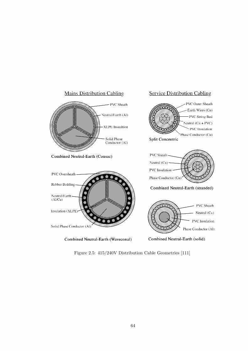
Figure 2.5: 415/240V Distribution Cable Geometries [111]

64

Concentric single phase service cables are straightforward to model in ATP-EMTP

as sheathed single core cables, assuming the stranded conductors to be solid tubular

sections of equal Cross-Section Area (CSA). Split concentric constructions can also be

accommodated by the use of an additional armour conductor for the earth wires. Cable

data used in this work as per [135,136] are provided in Appendix D

The modelling of 3-phase cables with concentric combined Neutral-Earth conductors

is considerably more difficult, mainly due to the sector geometry of the phase conductor

cross-section. As a rule, cable models in electromagnetic transients simulation software

pre-processors accept conductors of circular or tubular cross-section only, in order that

an analytical solution for the cable parameters may be easily obtained. A geometric

cable model accepting conductors of arbitrary shape and orientation would require an

intermediate finite element modelling stage in order to achieve similar results, adding

significant computational requirements to a given simulation. At present, no such

function is available to any of the ATP pre-processors, and an approximation to circular

conductor cross-section has been made where necessary.

2.4.3 Overhead Lines

The modelling of wood pole mounted bare-conductor overhead lines for rural distribution

networks is comparatively straightforward as the assumptions of carson’s equations are

easily satisfied. Aerial bundled conductor (ABC) lines common to rural 230/400V

circuits are somewhat less straightforward due to the effects of proximity between

phases.

Single and three-phase ABC conductors may be modelled using the LCC routine in

EMTP as unsheathed single sore cables in a close bundle as depicted by the cross-sections

of Figure 2.6 [139].

2.4.4 Transformers

All models used in this thesis consider the distribution network in detail up to the

11kV transformer. As such, the 415V winding of the transformer should be rendered

in detail, taking account of its winding impedances and stray capacitance, and also

including the inter-winding capacitive coupling to the 11kV primary.

65

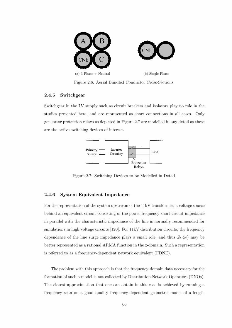
(a) 3 Phase + Neutral (b) Single Phase

Figure 2.6: Aerial Bundled Conductor Cross-Sections

2.4.5 Switchgear

Switchgear in the LV supply such as circuit breakers and isolators play no role in the

studies presented here, and are represented as short connections in all cases. Only

generator protection relays as depicted in Figure 2.7 are modelled in any detail as these

are the active switching devices of interest.

Figure 2.7: Switching Devices to be Modelled in Detail

2.4.6 System Equivalent Impedance

For the representation of the system upstream of the 11kV transformer, a voltage source

behind an equivalent circuit consisting of the power-frequency short-circuit impedance

in parallel with the characteristic impedance of the line is normally recommended for

simulations in high voltage circuits [120]. For 11kV distribution circuits, the frequency

dependence of the line surge impedance plays a small role, and thus ZC(ω) may be

better represented as a rational ARMA function in the z-domain. Such a representation

is referred to as a frequency-dependent network equivalent (FDNE).

The problem with this approach is that the frequency-domain data necessary for the

formation of such a model is not collected by Distribution Network Operators (DNOs).

The closest approximation that one can obtain in this case is achieved by running a

frequency scan on a good quality frequency-dependent geometric model of a length

66

or mesh of 11kV cable or OHL. Figure 2.8 illustrates the process of extracting the

frequency domain self- and mutual-impedance scan, to which rational functions Z(z)

may be fitted by linearised least-squares approximation as per [140,141].

Figure 2.8: Formation of an FDNE by Line Frequency Scan

2.5 Domestic/Commercial Wiring Installations

There follows a discussion of requirements for the modelling of cabling and load conditions,

for scenarios in which additional detail downstream of the customer supply point is

needed.

2.5.1 Cables and Distribution Boards

Early domestic cable models consisted of lumped equivalent PI sections, providing

reasonable results in simulations with time steps greater than 10ns. The drawback

with this approach is that the discrete components have to be evaluated individually

for each length and cross-section of cable, and are only correct at a single frequency. A

frequency dependent transmission line is therefore preferred, but given the prohibitively

short travel times between cable terminals, a different time step has been chosen for

the more detailed studies (see Table 2.1).

Assuming a propagation velocity equal to that of free space (νp = c), a travelling

wave line model at a solution time-step of 5ns can theoretically represent section lengths

as short as 3m. This reduces to approximately 1.6m if one assumes that all propagation

modes occur within the PVC insulation/sheath. Minimisation of interpolation errors

then dictates a practical lower limit of 8m for a single line section, which is considered

ample for the representation of typical domestic wiring circuits.

A library of flat and circular flex cable geometries, as depicted in Figure 2.9 has been

constructed using both modal- and phase- domain frequency dependent line models,

67

Figure 2.9: Domestic Cable Geometries

Figure 2.10: Linear and Non-Linear Load Representation

yielding very similar results.

2.5.2 Loads

Localised customer load is represented to varying degrees of detail as dictated by the

required time-step resolution of a given model. High resolution domestic circuit circuit

models in which mains cable runs are represented explicitly as travelling-wave models

(section 2.5.1) require that loads appearing on different mains and spurs be modelled

separately. A selection of linear and pseudo-nonlinear branches are used to represent

typical localised loads for different household occupancy scenarios.

Nonlinear load is modelled as an antiparallel arrangement of empirically defined

Shockley diode elements as depicted in Figure 2.10. Linear loads are supplemented

with shunt capacitance of 10-40pF, representing stray effects in adapters and power

supply circuitry. Nonlinear loads by contrast are assumed to possess significant input

capacitance allowing stray effects to be neglected.

In lower resolution models incorporating many customer nodes dispersed across

multiple LV feeders, the modelling of circuits downstream of the consumer unit becomes

68

impractical. Individual customer load must, therefore, be aggregated into a single

linear branch. Stray effects are still included, though supplemented with an additional

capacitance in place of the omitted cable spurs.

2.6 Small-scale Embedded Generation

2.6.1 Direct Connection

Direct-connected induction machine type sources, being limited to certain µCHP and

micro-wind designs, are taken to constitute only a small proportion of future installed

SSEG capacity. The specific characteristics of such generators have for this reason been

omitted from study, an exclusive adoption of converter-based devices being assumed.

2.6.2 Converter Interfaces

The necessary level of detail in modelling converter topologies is largely dictated by

its required degree of flexibility in application. A range of device equivalent circuits

have been developed, ranging from a simplistic representation of output filters and

capacitive inrush to complex explicit representation of power electronic circuits and

toroidal transformer saturation characteristics. A detailed discussion of each topology

and its applicability to the simulation of transient phenomena can be found in Chapter

5.

2.6.3 Switches and Disconnects

Main inverter disconnect relays are represented as ideal switches in parallel with their

nominal open-state stray capacitances, with contact resistance neglected. Power-electronic

switches are treated in a similar fashion, with the addition of on-state series resistance,

snubber circuitry and antiparallel diode branch as depicted in Figure 2.11. Discussion of

relay pole adaptation to statistical or systematic switches for the purpose of large-scale

repeat simulations is given in Chapter 6.

2.7 Chapter Conclusions

In this chapter, Dommel’s trapezoidal integration method for time-domain computation

of electromagnetic transients has been discussed. The merits and drawbacks of this

solution method have been evaluated, with particular consideration of solution accuracy,

69

Figure 2.11: Switch Representation by Type

stability and conditioning of the network conductance matrix. It was determined that

a discretisation based on trapezoidal integration, despite a propensity for giving rise

to numerical oscillation, was the best initial choice due to the inherent stability of the

resulting discrete system model.

Particular consideration has been given to difficulties in the modelling of low-voltage

network components, as distinct from those relating to MV and HV systems. Principal

considerations are time-step constraints due to propagation times in very short (of

the order of 10m) cables and lines and the handling of small circuit time constants;

non-circular cable geometries; and marginal satisfaction of the assumptions of Carson’s

equations due to the neglect of proximity effects.

In the light of such considerations, with the aid of laboratory test and manufacturers’

data, a library of low-voltage system components has been generated using the EMTP-ATP

graphical preprocessor ATPDraw. Transient characteristics of small distributed generators,

however, remain an unknown, necessitating the design and construction of a generator

test bed as discussed in the next chapter.

70

Chapter 3

Laboratory Rig for theEvaluation of MicrogenerationTransient Phenomena

The development of good predictive simulation models is heavily dependent on

the availability of field and laboratory test data. In the case of LV networks and

associated embedded generation technologies, the available data are somewhat

limited, with little or no data relating to electromagnetic transient phenomena. This

chapter details the design and construction of a laboratory test bed for the acquisition

of the necessary simulation model data.

3.1 Overview

The principal aim of the laboratory work undertaken was to study voltage and current

transients at the device terminals and consumer bus, arising due to switching of an

integrated protection relay as required by ENA ER G83-1 [5]. The chosen source

technology for this investigation was a solar photovoltaic energy system, as depicted

in Figure 3.1, which was constructed and tested within the Cardiff University Solar

Energy Laboratory.

The chosen solar inverter, as with all off-the-shelf SSEG grid interfaces, has an

integrated electromechanical protection relay and control system to facilitate disconnection

of the source from (and delayed reconnection to) the grid in response to voltage rise/dip,

frequency deviation and loss-of-mains scenarios as defined in G83-1. It is the operation

of this relay and any associated electrical transients that shall be of primary interest

71

Figure 3.1: Basic Test Layout of Rig Indicating the Switching Device of Interest

in this chapter. The laboratory rig design would therefore need to incorporate the

following components:

• A means of triggering inverter grid protection in a user-determinable manner;

• Steady-state measurement apparatus to record pre- and post-switch conditions;

• Transient measurement system capable of capturing and processing a wide range

of voltage and current waveform data, consisting of one or more transient peaks;

• Data acquisition system for the automated logging of large quantities of steady-state

and transient data.

3.2 Test and Equipment Specification

This section describes the specified laboratory test regimes, together with a breakdown

of key measurement criteria as derived from insulation coordination and electromagnetic

compatibility standards. Requirements of the test equipment, such as measurement

resolution and data handling capability, are then discussed.

3.2.1 Time-Domain I-V Measurement

In order to correctly characterise the transient behaviour of each switching event, a

comprehensive set of measurement criteria was established. These criteria serve to

maximise the data yield of a given test, thereby minimising the need for repetition

and allowing statistical methods to be applied. Using the standardised wave-shapes

from Insulation Coordination and EMC standards [137, 138, 142, 143] (Table 3.1) and

commonly used electromagnetic susceptibility test wave-shapes as in [81] (Table 3.2)

as reference, it was determined that the following data should be acquired for each

switching event:

72

• Peak transient voltages and currents (Vmax, Vmin, Imax, Imin) at the generator

terminals and consumer unit bus,

• Rate of rise of voltage and current fronts

(dVrisedt

,dIrisedt

)for both positive- and

negative-going transients,

• 50% values of voltage and current tails and rates of roll-off

(dVfalldt

,dIfalldt

),

• Switching delays (τsw) in operation of live and neutral relay poles, and any

subsequent transients due to inrush (τi),

• Instantaneous terminal voltage and timing of switching instants with respect to

the supply voltage sinusoid (tsw1, tsw2).

A sequence of transient events may be observed for each switching operation, due

to independent pole closing delays and the possible occurrence of capacitive inrush.

A sufficiently large time window would therefore be necessary to capture all of the

relevant data for each event. A suitable window was found experimentally to be around

20ms. It was anticipated that while relay pole operation might give rise to the fastest

transients, worst case current and voltage magnitudes would be associated with the

subsequent inrush. It was important, therefore, to quantify the magnitudes and relative

frequency of occurrence of any and all inrush events as these shall represent the most

onerous conditions with regard to insulation degradation, thermal overload and damage

to electronic components by induced effects.

The components of the electromagnetic immunity test waveshapes can be calculated

from acquired data using the relations in Table 3.2, where um is the peak value of the

transient,du

dtthe initial rate of rise and S the energy measure of the wave:

S =

∫ ∞0

u2(t)dt (3.1)

These measurements may either be interrogated in hardware at the time of test,

or sufficient waveform data should be stored such that the required values may be

extracted by post-processing. Figure 3.2 illustrates the measurement points of interest

on a generic waveform, with reference to one cycle of the 50Hz supply voltage.

Given the lack of pre-existing transient data, and the fact that electrical time

constants in an LV network are typically much shorter than those at medium and

73

Table 3.1: Transient Classes and Standard Test Waveshapes According to InsulationCoordination Standard BS EN 60071 [138]

Class Slow-Front Fast-Front Very-Fast-Front

TypicalWaveshapes

20µs < TP ≤ 5ms 0.1µs < T1 ≤ 20µs Tf < 100nsRange of 0.3MHz < f1 < 100MHzWaveshapes T2 < 20ms T2 < 300µs 30kHz < f2 < 300kHz

-StandardWaveshapes

Standard TP = 250µs T1 = 1.2µs -Values T2 = 2 500µs T2 = 50µs

Standard Switching Lightning -Test Impulse Test Impulse Test

74

Table 3.2: Common Electromagnetic Susceptibility Test Waveshapes [81]

Symmetric Trapezoidal Double Exponential Damped OscillatoryPulse (STP) Pulse (DEP) Wave (DOW)

- u(t) = AD

(e− tτd − e−

tτr

)u(t) =

umtat [0 ≤ t ≤ ta]

- - u = ume−α(t−ta) cos (ω(t−ta))

[t > ta]

um = AS um = AD ·r − 1

re−

ln(r)r−1 -

du

dt=ASta

du

dt=r − 1

τdAD -

S =

(th −

ta3

)A2S S =

τ(r − 1)2

2(r + 1)A2d S =

(ta3

+2α2 + ω2

4α(α2 + ω2)

)u2m

-

(r =

τdτr

)(ω = 2πfw)

75

Figure 3.2: Key Data Extraction from a Generic Event Record

high-voltage, the data acquisition equipment was specified to achieve the maximum

possible bandwidth. Post-processing of very large data files was deemed undesirable,

and a direct extraction of characteristic values in hardware preferred wherever feasible.

3.2.2 Test Scenarios

A primary requirement of the laboratory study was to quantify the dependence of

transient currents and voltages on instantaneous local loading, and on distance of the

connection point from the 11kV transformer. As such, the test rig was designed to

include a variable local dump load, and a range of possible fault levels at the consumer

bus. In addition, all tests were specified to perform switch timing and delay analyses

on the acquired data. Three principal test configurations were specified in order to

quantify the following:

• Transient voltages and currents generated on disconnection of the inverter from

the mains supply.

• Transient voltages and currents generated on reconnection to the supply.

• The effect of supply impedance on the magnitudes of these transients.

76

Details of the rig components and equipment capabilities are given in sections 3.4

and 3.5. The specifics of each testing configuration are covered in detail in Chapter 4

3.2.3 Statistical Analyses

Simulations of individual timed switching events provide useful pointers to the transient

phenomena of interest, but the information that these simulations provide is minimal,

and in many cases represents a worst-case scenario which itself may occur too infrequently

to be of any concern. Far more useful information can be obtained by performing

a sequence of simulations in which the operation of switches in successive re-runs is

governed by a statistical distribution in time. This is of particular use when multiple

devices are operating on a single network in response to a common stimulus, each with

their own pole operation delay.

In order to inform such simulations, sufficient statistical data must be obtained by

laboratory test under repeatable conditions. A large number of events must be recorded

in order that the statistical distributions governing the switch pole operation may be

extracted, and minimisation of total lab time requires that all test scenarios be specified

to generate this timing data. Being confined to a single test rig and lacking any external

source of additional data, the amount of statistical information that could be extracted

was somewhat limited due to the time-consuming nature of the acquisition process.

3.2.4 Repeatability

It was determined that all testing and data acquisition be performed on a complete

system rather than using a representative source behind a grid inverter, so as to be

able to fully mimic source-device interaction in subsequent simulations. Given the

present drive towards expansion in small grid-tied photovoltaic systems in the UK,

this form of generation was deemed most appropriate for study, and a small test rig

constructed (section 3.4). In order to collect useful laboratory data on a systematic

basis, external variables such as temperature, irradiance and airflow had to remain as

constant as possible for the duration of a test, allowing electrical phenomena to be

observed in isolation. Outdoor testing was deemed unfavourable in the short-term due

to variability of conditions, and it was decided that all testing be undertaken within

the School of Engineering’s Solar Energy Laboratory.

77

3.3 The Solar Energy Laboratory

The Solar Energy Laboratory at Cardiff University is a dedicated environment for the

evaluation and testing of full-scale solar thermal and photovoltaic systems in situ, under

repeatable controlled conditions. The laboratory’s main feature is a manoeuvrable array

of 36 parabolic Compact Iodide Daylight (CID) lamps, shown in operation in Figure

3.3. The lamps are arranged in a square array, measuring 2.85m x 2.85m between

corner beam centers, and at a distance of 5.2m from target illuminates an area of

approximately 10m2 at a spectral intensity in excess of 400W/m2.

Figure 3.3: CID Lamp Array in the Solar Energy Laboratory

The use of narrow beam angles results in considerable hot-spot formation, and peak

intensities at the center of the target area are typically above 700W/m2. A number

of broadband irradiance tests were performed using a pyranometer placed at 25 evenly

spaced points in a plane perpendicular to the angle of incidence. The results of these

tests were used to determine the optimal size and position of a test rig, and the radiation

flux density at the surface of the chosen configuration is shown in Figure 3.4.

3.3.1 Lamps

The lamps used are 1000W Cold-restrike narrow-spot CIDs with 8-inch parabolic

reflectors. These produce a spectrum comparable to that of direct solar radiation,

78

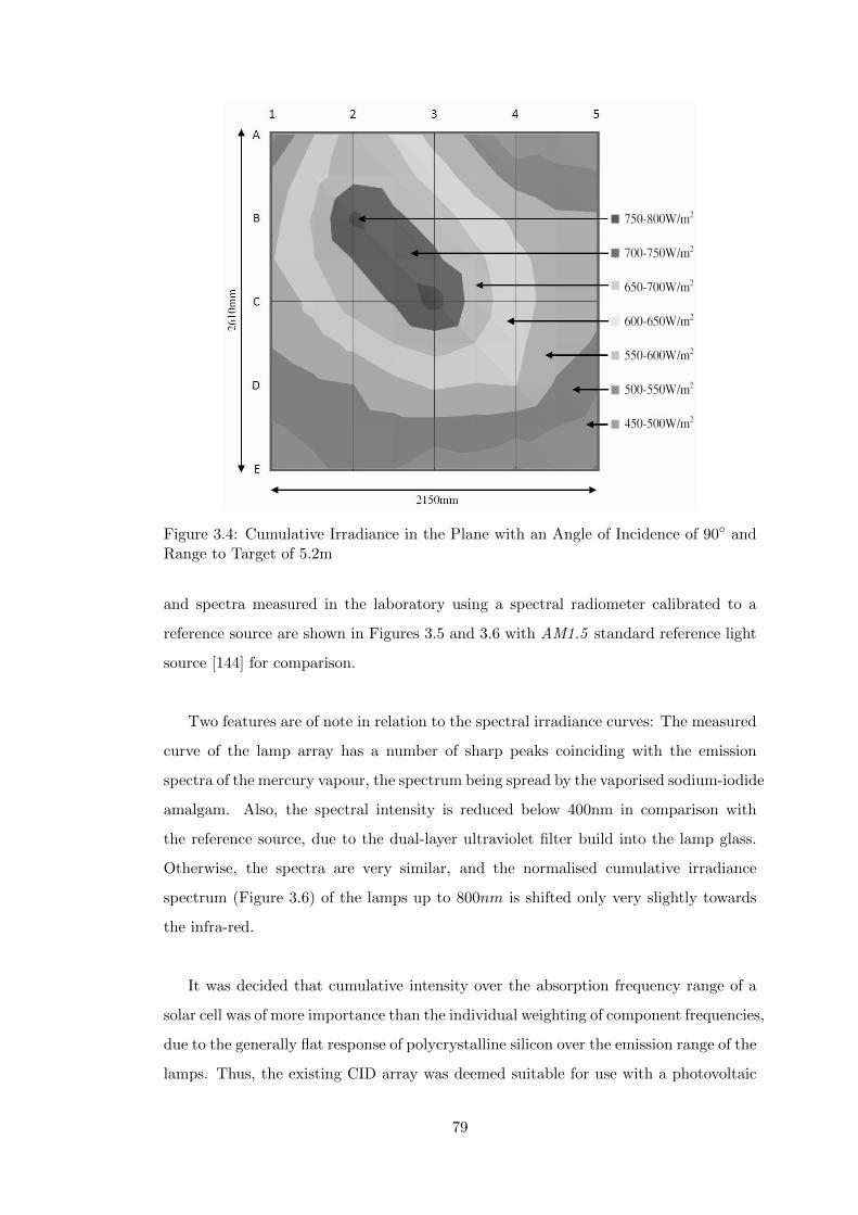
Figure 3.4: Cumulative Irradiance in the Plane with an Angle of Incidence of 90 andRange to Target of 5.2m

and spectra measured in the laboratory using a spectral radiometer calibrated to a

reference source are shown in Figures 3.5 and 3.6 with AM1.5 standard reference light

source [144] for comparison.

Two features are of note in relation to the spectral irradiance curves: The measured

curve of the lamp array has a number of sharp peaks coinciding with the emission

spectra of the mercury vapour, the spectrum being spread by the vaporised sodium-iodide

amalgam. Also, the spectral intensity is reduced below 400nm in comparison with

the reference source, due to the dual-layer ultraviolet filter build into the lamp glass.

Otherwise, the spectra are very similar, and the normalised cumulative irradiance

spectrum (Figure 3.6) of the lamps up to 800nm is shifted only very slightly towards

the infra-red.

It was decided that cumulative intensity over the absorption frequency range of a

solar cell was of more importance than the individual weighting of component frequencies,

due to the generally flat response of polycrystalline silicon over the emission range of the

lamps. Thus, the existing CID array was deemed suitable for use with a photovoltaic

79

Figure 3.5: Spectral Irradiance of Lamp Array, Scaled for a Cumulative Total of1000Wm−2 (AM1.5 Spectrum [144] for Comparison)

rig, with the condition that the rig be placed far enough from the lamps to avoid cell

damage due to hot-spot formation.

3.3.2 Ignition and Control

The intensity and lifetime of metal-halide discharge lamps are sensitive to deviation

of terminal voltage from their rating. To minimise the effect of the high supply

voltage (typically in excess of 420V , 3-phase), as well as more short-term variability,

the lamp-ballast and ignition circuits are fed from a stabilised supply configured to

supply the lamps at their rated voltage. In addition, single phase variacs are provided

downstream of the stabilisers, to provide a degree of individual lamp brightness control.

Because the lamps have a very limited dimming capability, the usefulness of individual

control variacs is limited. It was not possible to repeat experiments for a range

of irradiance levels, and small adjustments were made only periodically in order to

counteract the natural dulling that occurs with with lamp ageing.

Finally, lamp ignition is performed by individual 12kV igniters housed at the rear

of each lamp assembly. Lamps are fired in groups of three from ignition switches

mounted on the wall of the laboratory, and once ignited are subject to a 30-minute

power cycle before re-ignition. This condition was found to be the principal cause of

80

Figure 3.6: Normalised Cumulative Irradiance of Lamp Array from 280nm to 800nm(AM1.5 [144] for Comparison)

delay in extended test regimes, as a misfired lamp requires those already lit to be fully

cycled before a second attempt can be made. A proposal was drafted by the author for

conversion of the CID array to equivalently rated parabolic halogens utilising a stage

lighting system, which would eliminate time-consuming power cycling requirements and

allow for dynamic variation in light intensity during future tests (see Appendix E).

3.3.3 Orientation and Manoeuvrability

Positioning of the lamp array is achieved by use of two travelling crane hoists running

on I-beams in the ceiling space of the laboratory. Once in position, the array must be

anchored by means of fixed load-bearing chains so as not to statically load the crane

clutch. Verical and Horizontal manoeuvring of the array during test is therefore not

possible, and a suitable fixed position of the tilt axis was determined for all tests. The

tilt angle and lamp rotation were then adjusted in order to align with the test object.

In order to maximise the beam spread, and thereby minimise hotspot formation, the

full length of the laboratory was utilised. A tilt angle of 36 was found to satisfy this

condition, and kept fixed for the duration of testing. Thus a fixed tilt angle could also

be specified for the photovoltaic array, discussed in the next section. The laboratory

configuration is shown diagrammatically in Figure 3.7

81

Figure 3.7: Position and Orientation of CID Array and Target

3.4 Photovoltaic Array Test Rig

3.4.1 Panels

Economical use of the illuminable area was made using an array of BP Solar 380J

multi-crystalline silicon-nitride PV panels [145]. The panels were arranged in a 4 × 2

array, measuring 2150mm by 2690mm with a total cell surface area of 4.80m2. These

were mounted on a lightweight frame constructed from 30 × 30mm and 45 × 45mm

modular aluminium section, as shown in Figure 3.8. Manoeuvrability was achieved by

mounting on antistatic castors, and a sliding hinged frame construction was chosen to

allow minor adjustment of the tilt angle (36 ± 5).

82

Figure 3.8: Photovoltaic Array and Mounting

The panels were string-connected to form an array with a nominal rating of 640W

under standard test conditions (1000W/m2 AM1.5 spectrum, 20C air temperature).

Due to a reduced and uneven distribution of radiation emitted by the lamps, and an

elevated air temperature typically around 25C, the peak output power was reduced

to approximately 350W as shown in the array I-V curve of Figure 3.9. Operation at

the maximum power point (MPP) at an air-temperature of 25C generated a current of

2.83A at a terminal voltage of 123.3V DC. System open circuit voltage was approximately

151.1V, while short-circuit current was measured at 4.64A, slightly above its nominal

value of 4.55A.

3.4.2 Inverter

Output current from the array was fed to an SMA SunnyBoyTM 700 Grid Inverter,

mounted on a moveable trolley as shown in Figure 3.10. The inverter input MPP

voltage range was set to 100-160V for a peak theoretical efficiency of 93.3%. The AC

terminals were connected through a 16A miniature circuit breaker (MCB) to a 16m

83

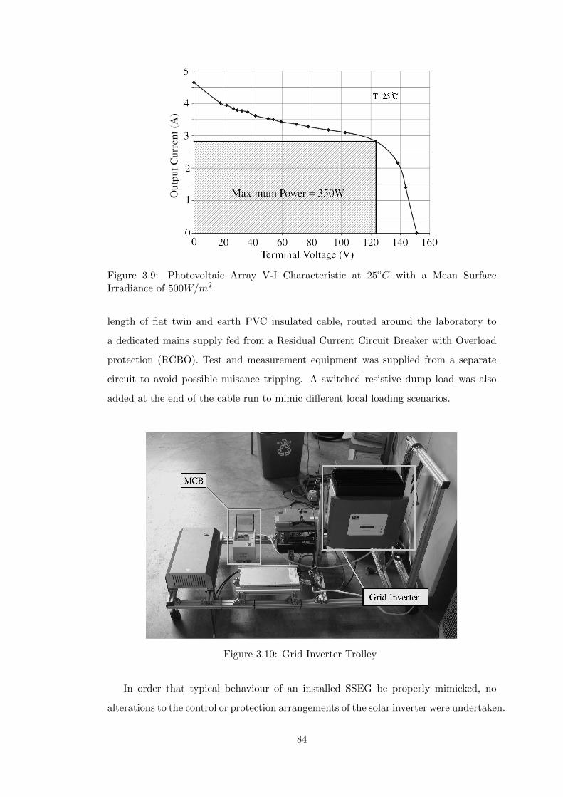
Figure 3.9: Photovoltaic Array V-I Characteristic at 25C with a Mean SurfaceIrradiance of 500W/m2

length of flat twin and earth PVC insulated cable, routed around the laboratory to

a dedicated mains supply fed from a Residual Current Circuit Breaker with Overload

protection (RCBO). Test and measurement equipment was supplied from a separate

circuit to avoid possible nuisance tripping. A switched resistive dump load was also

added at the end of the cable run to mimic different local loading scenarios.

Figure 3.10: Grid Inverter Trolley

In order that typical behaviour of an installed SSEG be properly mimicked, no

alterations to the control or protection arrangements of the solar inverter were undertaken.

84

The integrated protection was permitted to disconnect the device from the supply in

response to voltage deviations and loss-of-mains, in the same manner as would occur

in a normal domestic installation. Controlled disconnection was achieved indirectly

by manipulation of the incoming mains supply voltage, rather than by direct manual

operation of the protection relays. The pre-set delay in the relay open/close cycle was

also preserved to allow realistic settling time for the DC bus capacitance post-disconnect.

3.5 Test and Measurement Equipment

The following section briefly discusses the measurement equipment specifications for the

laboratory, and provides a breakdown of devices used and their key features. Detailed

equipment information can be found in Appendix B. Equipment may be broadly split

into two categories according to resolution; one for steady state applications (monitoring)

and the other for high speed transient data capture.

3.5.1 Steady-State Monitoring

Continuous monitoring of the voltages and currents in the test system is necessary in

order that switching operations may be repeated from the same initial state, and to

allow relation of transient measurements to prior steady-state conditions.

3.5.1.1 Probes and Meters

Voltage and current measurements on the array DC bus were made using LeCroy

SI-9000 200:1 differential voltage and LEM PR20 20kHz multimeter AC/DC current

probes. A second, identical pair of probes were used for monitoring of the AC voltage

and current at the inverter terminals. Steady-state voltage and current measurement at

the load was performed by a Keithley 2000 Multimeter and a third LEM PR20 current

probe.

The current and voltage probes were connected in differential mode to analogue

input channels 0 to 4 of a USB data-acquisition board, while the multimeter was

connected to the PC via a National InstrumentsTM GPIB-USB converter. The set-up

is illustrated in Figure 3.11.

85

Figure 3.11: Complete Laboratory Equipment Set-up, Indicating the SwitchingOperation of Interest

3.5.1.2 Data-acquisition Board

An NI USB-6212 400kS/s multifunction data-acquisition (DAQ) board with 16-bit input

ADC was used for the collection of steady-state system data. All probes were connected

to the DAQ via a connector box and short lengths of 0.23mm2 foil-shielded twisted pair

cable. The signal lines were terminated in differential mode with 100kΩ resistor pairs

between each channel and the earth reference of the DAQ.

3.5.2 Fast Transient Measurement

A second set of measurement equipment was specified for the high-frequency measurement

of transients, as can also be seen in Figure 3.11.

3.5.2.1 Voltage Probes

Voltage transients were measured at the inverter AC terminals and consumer unit

bus using a pair of Pintek DP-25 differential probes. These probes have a low input

capacitance (1.2pF differential, 3.7pF common), and a -3dB bandwidth of 25MHz at

an attenuation setting of 200:1.

86

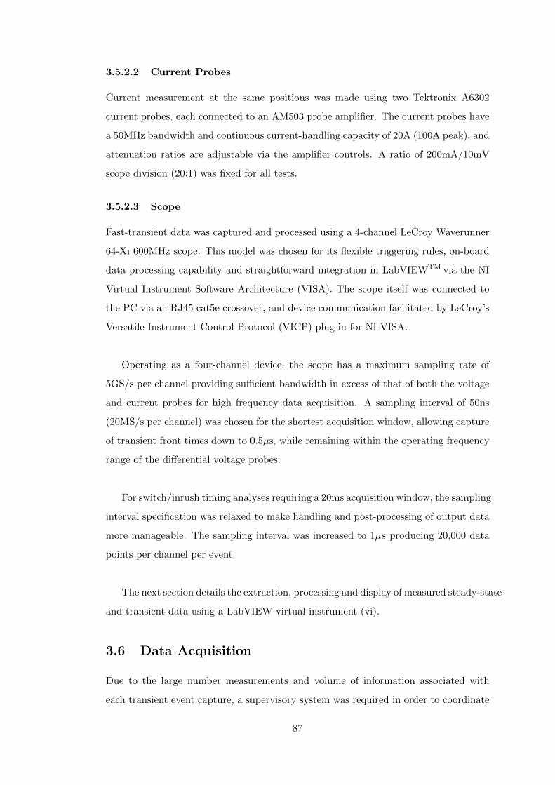
3.5.2.2 Current Probes

Current measurement at the same positions was made using two Tektronix A6302

current probes, each connected to an AM503 probe amplifier. The current probes have

a 50MHz bandwidth and continuous current-handling capacity of 20A (100A peak), and

attenuation ratios are adjustable via the amplifier controls. A ratio of 200mA/10mV

scope division (20:1) was fixed for all tests.

3.5.2.3 Scope

Fast-transient data was captured and processed using a 4-channel LeCroy Waverunner

64-Xi 600MHz scope. This model was chosen for its flexible triggering rules, on-board

data processing capability and straightforward integration in LabVIEWTM via the NI

Virtual Instrument Software Architecture (VISA). The scope itself was connected to

the PC via an RJ45 cat5e crossover, and device communication facilitated by LeCroy’s

Versatile Instrument Control Protocol (VICP) plug-in for NI-VISA.

Operating as a four-channel device, the scope has a maximum sampling rate of

5GS/s per channel providing sufficient bandwidth in excess of that of both the voltage

and current probes for high frequency data acquisition. A sampling interval of 50ns

(20MS/s per channel) was chosen for the shortest acquisition window, allowing capture

of transient front times down to 0.5µs, while remaining within the operating frequency

range of the differential voltage probes.

For switch/inrush timing analyses requiring a 20ms acquisition window, the sampling

interval specification was relaxed to make handling and post-processing of output data

more manageable. The sampling interval was increased to 1µs producing 20,000 data

points per channel per event.

The next section details the extraction, processing and display of measured steady-state

and transient data using a LabVIEW virtual instrument (vi).

3.6 Data Acquisition

Due to the large number measurements and volume of information associated with

each transient event capture, a supervisory system was required in order to coordinate

87

the triggering and data-extraction processes. A transient logger was constructed using

LabVIEW for the processing and storage of steady-state and transient data extracted

via the DAQ and Oscilloscope.

3.6.1 Requirements

It was decided that the transient logger should perform the following broad functions:

1. Steady-state monitoring of array and inverter currents, voltages and power flows

for the full duration of a test.

2. Display captured transient waveforms on an event-by-event basis.

3. Provide visual indication of measurement system status and prompt for action

following triggering events.

4. Allow remote re-arming of all triggers from inside the execution loop.

5. Facilitate the extraction and storage of data, either by generating new files or

appending to an existing dataset.

3.6.2 Program Overview

The transient logger vi consists of a tabbed display, with controls and indicators

assigned to pages by function. The tabs are broken down as follows:

• Inputs: For the specification of measurement equipment set-up parameters prior

to test.

• Execution: Provides rolling display of steady-state measurements and trigger

event feedback during the test.

• Error Handling : Gathers error log information at key stages of the program

execution loop.

3.6.2.1 Inputs

The Inputs panel is shown in Figure 3.12. This screen allows the user to enter information

such as the attenuation settings of voltage and current probes, the desired scope set-up

parameters (time-base, vertical scale, sample size, trigger levels) and DAQ card set-up

(sampling rates, scaling, number of cycles recorded per sweep). The number of events

88

to be recorded in a test session may be specified, as well as the location to which output

data is to be saved (either to a new file, or appended to an existing data set).

Figure 3.12: Input Pane

3.6.2.2 Execution

The Execution panel is shown in Figure 3.13. When a test is being performed, this pane

provides a continuously updating display of the steady state operation of the system,

allowing the user to ensure switching of the generator disconnect only after steady state

operation has been reached. Steady state monitoring is performed with the visual aid

of the left-hand charts, while the right-hand side displays transient waveforms from the

previous event as a visual review.

The DC power output of the PV array, AC real power output of the inverter and

load power are calculated internally using the power analyser module and displayed,

together with converter efficiency and export power factor. An indicator is provided

to inform the user when the system is fully grid-connected and exporting power. Only

under such conditions should a new fault event be initiated, so this feature helps to

minimise the duration of a test. Similarly, indication is provided when the trigger state

89

Figure 3.13: Execution Pane

of the scope changes, allowing the user to verify captured data before it is stored.

After testing numerous versions of the vi during its development stage, it was

decided that a manual approval mechanism for the storage of event data was the

most robust approach, even if initially it is time-consuming. The sensitive trigger

requirements of certain tests gave rise to a significant number of nuisance events,

while others were missed entirely due to ill-defined glitch trigger set-up. No optimal

triggering regime could be identified such that only useful data was produced, limiting

the applicability of a fully automated data logging system. This was only of minor

inconvenience, as user input was still necessary to initiate successive transients.

3.6.3 DAQ Program Execution Structure

Figure 3.14 summarises the execution structure of the transient data logger vi. Once

initial set-up parameters have been specified by the user, a run command will initialise

the scope and DAQ card before dropping in to a loop in which steady-state monitoring

data is collected and refreshed. On closing the MCB, the inverter will remain disconnected

for three minutes as a safety precaution. This is followed by a short period of grid

monitoring (typically around 20s) before the GridGuardTM disconnectors close.

90

Triggering of the scope due to this switching operation is flagged to the user, who

must verify that correct triggering has occurred. If so, the program execution breaks

out of the steady-state loop and continues to the data extraction stage, otherwise the

scope is manually re-armed from the execution panel and the program continues to wait

for an event.

The data extraction stage involves interrogation of the waveforms within the scope

software to retrieve the following measurements:

• Peak currents and voltages: Vmax, Vmin, Imax, Imin

• Rise time of the front: Tr 20−80%, Tr 10−90%, Tr 30−90%

• Fall time of the tail: Tf 80−20%, Tf 90−10%, Tf 90−30%

• Maximum rate of change:dV

dt

∣∣∣∣max

,dI

dt

∣∣∣∣max

• Energy content of the transient: W ≈∫ T

0(v · i) dt

• Energy measure of the transient: Sv ≈∫ T

0v2(t) dt, Si ≈

∫ T

0i2(t) dt

On the first recorded event, the user is either prompted for a new measurement file

name, or to identify an existing file to append, and measurements of subsequent events

are automatically appended to the same file. The raw waveforms are also time-stamped

and saved to auxiliary data files, with descriptive file names generated from that of the

parent measurement file.

Once the transfer to the data logging PC is complete, the event count is incremented

and if the requested number has been reached, the program exits with a visual indicator

signifying successful completion. Otherwise, the scope is re-armed and the program

returns to the steady-state monitoring loop to await the next trigger event. The

program may be halted manually at any point if necessary.

3.6.4 Data Files

Measurement and Raw Data files are saved as comma-separated variable (csv) files for

simple post-processing in Matlab or Excel. If a new file is to be created, the first storage

91

Figure 3.14: Execution Structure of the LabVIEW Data Acquisition vi

92

request will prompt for a file name for the measurement file. The program will then

create a set of raw data files by appending a descriptive string to this file name, and

saving these to the same folder. For example, a measurement file name "file1.csv"

will generate auxiliary files "file1_Vsource.csv", "file1_Vload.csv"... for each of

the transient data acquisition channels.

3.7 Data Post-processing

Fast transient waveforms captured using the scope fall into one of two categories:

1. Single-peak snapshots for determining peak values and rates of change at high

precision.

2. Dual-peak capture for switch timing analysis, determination of switch pole delay

and transformer current inrush measurement.

Interrogation of single-peak waveforms, such as that shown in Figure 3.15, is a simple

process, and the measurements identified on page section 3.6.3 can all be extracted in

the scope hardware before the data is transferred to the PC for storage. A sub-vi

within the data-acquisition program was written in order to perform this interrogation

procedure, thus minimising the amount of post-processing of raw data required.

For the identification of timing of transient fronts with respect to the supply voltage

sinusoid, a longer capture window of 20ms is necessary. Within this window, a pair

of transients of opposing polarity are normally observed as shown in Figure 3.16,

from which the required timing information can be extracted. Due to the variation

in switch pole delay τsw and inrush delay τi between successive tests, evaluation of

these quantities using scope hardware was found to be unreliable. Determining the

amplitudes and rise/fall-times of the secondary peak was thus inconsistent, and as

such, all waveform captures with multiple peaks required further post-processing to

complete the measurement data set.

This section details the post-processing operations undertaken in order to generate

measurement sets from raw waveforms.

93

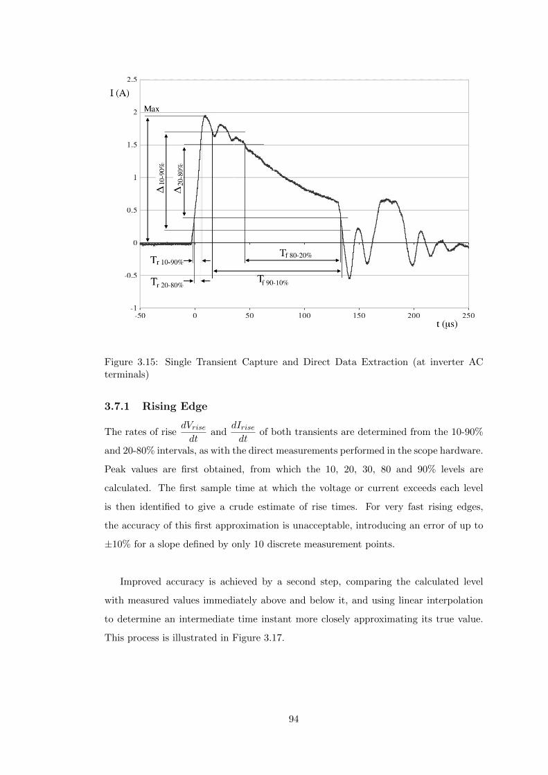
Figure 3.15: Single Transient Capture and Direct Data Extraction (at inverter ACterminals)

3.7.1 Rising Edge

The rates of risedVrisedt

anddIrisedt

of both transients are determined from the 10-90%

and 20-80% intervals, as with the direct measurements performed in the scope hardware.

Peak values are first obtained, from which the 10, 20, 30, 80 and 90% levels are

calculated. The first sample time at which the voltage or current exceeds each level

is then identified to give a crude estimate of rise times. For very fast rising edges,

the accuracy of this first approximation is unacceptable, introducing an error of up to

±10% for a slope defined by only 10 discrete measurement points.

Improved accuracy is achieved by a second step, comparing the calculated level

with measured values immediately above and below it, and using linear interpolation

to determine an intermediate time instant more closely approximating its true value.

This process is illustrated in Figure 3.17.

94

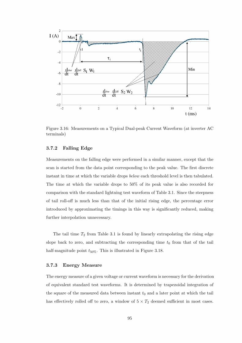
Figure 3.16: Measurements on a Typical Dual-peak Current Waveform (at inverter ACterminals)

3.7.2 Falling Edge

Measurements on the falling edge were performed in a similar manner, except that the

scan is started from the data point corresponding to the peak value. The first discrete

instant in time at which the variable drops below each threshold level is then tabulated.

The time at which the variable drops to 50% of its peak value is also recorded for

comparison with the standard lightning test waveform of Table 3.1. Since the steepness

of tail roll-off is much less than that of the initial rising edge, the percentage error

introduced by approximating the timings in this way is significantly reduced, making

further interpolation unnecessary.

The tail time T2 from Table 3.1 is found by linearly extrapolating the rising edge

slope back to zero, and subtracting the corresponding time t0 from that of the tail

half-magnitude point t50%. This is illustrated in Figure 3.18.

3.7.3 Energy Measure

The energy measure of a given voltage or current waveform is necessary for the derivation

of equivalent standard test waveforms. It is determined by trapezoidal integration of

the square of the measured data between instant t0 and a later point at which the tail

has effectively rolled off to zero, a window of 5 × T2 deemed sufficient in most cases.

95

Figure 3.17: Linear Interpolation Process for Determining Slope and Rise Time ofFast-front Transients

The integration in Equation (3.2) was performed for both transients in each captured

waveform, where ∆t represents the sampling interval of the oscilloscope. The process

is illustrated in Figure 3.19.

Sv =

∫ t0+5·T2

t0

v2(t) dt =

5·T2∆t∑n=1

v2[(n− 1)∆t+ t0] + v2[n∆t+ t0]

2

·∆t (3.2)

3.7.4 Energy Content

The energy content W is determined in a similar manner, except that it is calculated

from a third waveform p(t), which is simply the product of the coincident instantaneous

values of v(t) and i(t). This waveform is then numerically integrated over the same

time window as used for the energy measure S.

W =

∫ t0+5·T2

t0

p(t) dt =

5·T2∆t∑n=1

p[(n− 1)∆t+ t0] + p[n∆t+ t0]

2

·∆t (3.3)

3.7.5 Switch/Inrush Timing and Delay

The timing of switch operation and inrush inception relative to the zero-crossing of

the grid reference sinusoid can be determined by interrogation of the inverter terminal

current and voltage waveforms. No point-on-wave control of the relay closing operation

96

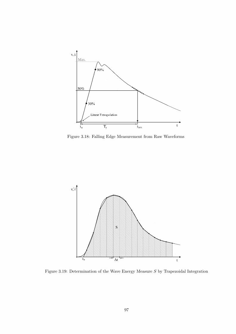
Figure 3.18: Falling Edge Measurement from Raw Waveforms

Figure 3.19: Determination of the Wave Energy Measure S by Trapezoidal Integration

97

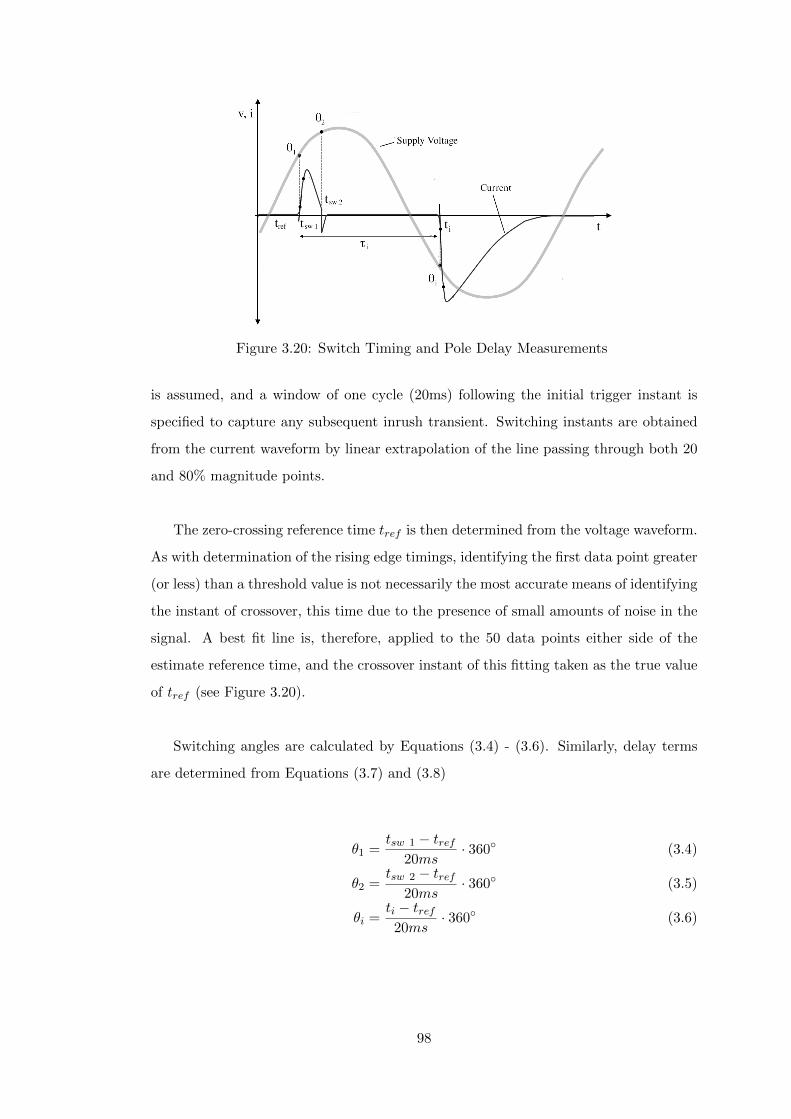
Figure 3.20: Switch Timing and Pole Delay Measurements

is assumed, and a window of one cycle (20ms) following the initial trigger instant is

specified to capture any subsequent inrush transient. Switching instants are obtained

from the current waveform by linear extrapolation of the line passing through both 20

and 80% magnitude points.

The zero-crossing reference time tref is then determined from the voltage waveform.

As with determination of the rising edge timings, identifying the first data point greater

(or less) than a threshold value is not necessarily the most accurate means of identifying

the instant of crossover, this time due to the presence of small amounts of noise in the

signal. A best fit line is, therefore, applied to the 50 data points either side of the

estimate reference time, and the crossover instant of this fitting taken as the true value

of tref (see Figure 3.20).

Switching angles are calculated by Equations (3.4) - (3.6). Similarly, delay terms

are determined from Equations (3.7) and (3.8)

θ1 =tsw 1 − tref

20ms· 360 (3.4)

θ2 =tsw 2 − tref

20ms· 360 (3.5)

θi =ti − tref

20ms· 360 (3.6)

98

τsw = tsw 2 − tsw 1 (3.7)

τi = ti − tsw 1 (3.8)


Characterisation of switching transients associated with SSEG disconnect and reconnect

operations is vital to the development of good simulation models. Details of a laboratory

test bed for the acquisition and analysis of switching transient magnitude, waveshape

and energy content under repeatable conditions and according to existing Insulation

Coordination standards have been presented. A complete photovoltaic installation

was designed and installed in the Cardiff University Solar Energy Laboratory, and a

semi-automated data-logging system constructed using NI LabVIEW for the acquisition

of generator transient data.

A variety of appropriate synthetic waveshapes has been proposed for the emulation

of typical waveforms in future time-domain simulation studies and laboratory tests. A

discussion of the results obtained from laboratory testing may be found in the chapter

that follows.

99

Chapter 4

Statistical Switching TransientMeasurements of a Solar EnergyInverter Source

In this chapter, results of laboratory experiments are presented with reference to

specific test configurations. Data are presented in such a way as to inform the

detailed simulation models of Chapters 5 and 6, and simple simulation results

accompany measurements where appropriate. To aid in the development of the software

models, experimental waveforms are compared with standardised test waveshapes in

order to identify the most appropriate transient source representations for future study.

4.1 Background

Connection of embedded generation rated below 16A per phase into the public electricity

supply is admissible subject to the given installation satisfying the connection requirements

in BS EN 50438 [6]. An important requirement of this document is that a generator

must disconnect from the grid in response to voltage and/or frequency excursions, as

summarised in Table 4.1. These requirements are equivalent to those laid out in Energy

Networks Association (ENA) Engineering Recommendation G83-1 [5].

Disconnection must be achieved by means of a two-pole electromechanical relay, such

that the device is fully isolated from the grid in the event of a fault on the supply side of

the consumer bus. Following restoration of the supply voltage and frequency to within

the allowable ranges defined in Table 4.1, a grid monitoring system shall wait a pre-set

time before re-closing the relay poles. This delay may vary from 20s for a low-inertia

100

Table 4.1: Disconnection Requirements of BS EN 50438 [6] and ER G83-1 [5]

Protection Setting Max. Clearance Time (s) Max. Trip Setting

Overvoltage (stage 1) 1.5 264V (+15%)Undervoltage (stage 1) 1.5 207V (-10%)Overfrequency 0.5 50.5Hz (+1%)Underfrequency 0.5 47Hz (-6%)Loss of Mains 0.5 -

device such as a grid inverter, to 3 minutes or more for a small induction generator,

but factory settings of like devices are typically uniform and remain unchanged once

installed.

Low voltage feeders with high penetration of embedded generation below 16A/phase

shall, therefore, be subject to multiple simultaneous or near-simultaneous switching

events in response to individual voltage or frequency excursions, with potential for

associated electromagnetic switching transients and transformer inrush. The purpose

of the laboratory experiments presented here is to understand and quantify the transient

characteristics of individual embedded generators over the disconnect/reconnect cycle.

The results shall help inform subsequent transient simulations with increased numbers

of devices, such that the cumulative effects of clustered generation may be predicted.

4.2 Laboratory Test Configurations

This section summarises variations in the detailed equipment specification discussed in

section 3.5, for the purpose of acquiring a range of data sets. For clarity, alterations

to the standard configuration are illustrated with the use of one-line diagrams. In all

cases, the solar array is connected to the inverter and available for generation.

4.2.1 Transients on Generator Reconnection

The generator was connected to the LV supply by 16m of 2.5mm2 twin and earth

cable, with a switch and MCB for protection and isolation, as shown in Figure 4.1.

Initial disconnection of the generator is achieved by a loss-of-mains (LoM) trip, initiated

by manual opening of the circuit breaker. Supply to the generator terminals is then

restored, and the transient logger armed to await reclosing of the disconnector.

101

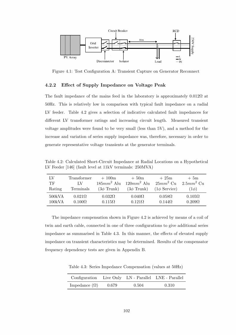
Figure 4.1: Test Configuration A: Transient Capture on Generator Reconnect

4.2.2 Effect of Supply Impedance on Voltage Peak

The fault impedance of the mains feed in the laboratory is approximately 0.012Ω at

50Hz. This is relatively low in comparison with typical fault impedance on a radial

LV feeder. Table 4.2 gives a selection of indicative calculated fault impedances for

different LV transformer ratings and increasing circuit length. Measured transient

voltage amplitudes were found to be very small (less than 5V), and a method for the

increase and variation of series supply impedance was, therefore, necessary in order to

generate representative voltage transients at the generator terminals.

Table 4.2: Calculated Short-Circuit Impedance at Radial Locations on a HypotheticalLV Feeder [146] (fault level at 11kV terminals: 250MVA)

LV Transformer + 100m + 50m + 25m + 5m

TF LV 185mm2 Alu 120mm2 Alu 25mm2 Cu 2.5mm2 CuRating Terminals (3φ Trunk) (3φ Trunk) (1φ Service) (1φ)

500kVA 0.021Ω 0.032Ω 0.040Ω 0.058Ω 0.105Ω100kVA 0.100Ω 0.115Ω 0.121Ω 0.144Ω 0.209Ω

The impedance compensation shown in Figure 4.2 is achieved by means of a coil of

twin and earth cable, connected in one of three configurations to give additional series

impedance as summarised in Table 4.3. In this manner, the effects of elevated supply

impedance on transient characteristics may be determined. Results of the compensator

frequency dependency tests are given in Appendix B.

Table 4.3: Series Impedance Compensation (values at 50Hz)

Configuration Live Only LN - Parallel LNE - Parallel

Impedance (Ω) 0.679 0.504 0.310

102

Figure 4.2: Test Configuration B: Determining Impact of Supply Impedance

4.2.3 Transients on Generator Disconnection

The capture of transients associated with the disconnection of the generator under

export conditions requires that the mains supply to the terminals remain live during

the entire switching cycle. A protection mechanism other than the LoM trip must,

therefore, be triggered, by either voltage or frequency deviation beyond the limits

defined in [5]. A variable transformer was employed to shift the feeder voltage beyond

the threshold levels dictated in Table 4.1, as illustrated in Figure 4.3.

Figure 4.3: Test Configuration C: Transient Capture on Generator Disconnect

Extensive testing using configuration C produced no significant results relating to

the disconnection of the generator. This is attributable to the fact that the solar inverter

feeds a predominantly resistive supply circuit, and operates close to unity power factor.

Current interruption therefore occurs near zero on the voltage sinusoid, and transient

recovery voltages are accordingly negligible. As a result, the sections that follow are

focused on re-closing operation of the inverter relay disconnect.

4.3 Experimental Results

The following section presents results of transient measurements made on reconnection

of the grid inverter to the LV supply. Results are presented in the following subsections:

• Current Measurements

103

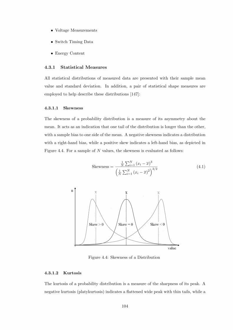
• Voltage Measurements

• Switch Timing Data

• Energy Content

4.3.1 Statistical Measures

All statistical distributions of measured data are presented with their sample mean

value and standard deviation. In addition, a pair of statistical shape measures are

employed to help describe these distributions [147]:

4.3.1.1 Skewness

The skewness of a probability distribution is a measure of its asymmetry about the

mean. It acts as an indication that one tail of the distribution is longer than the other,

with a sample bias to one side of the mean. A negative skewness indicates a distribution

with a right-hand bias, while a positive skew indicates a left-hand bias, as depicted in

Figure 4.4. For a sample of N values, the skewness is evaluated as follows:

Skewness =1N

∑Ni=1 (xi − x)3(

1N

∑Ni=1 (xi − x)2

)3/2(4.1)

Figure 4.4: Skewness of a Distribution

4.3.1.2 Kurtosis

The kurtosis of a probability distribution is a measure of the sharpness of its peak. A

negative kurtosis (platykurtosis) indicates a flattened wide peak with thin tails, while a

104

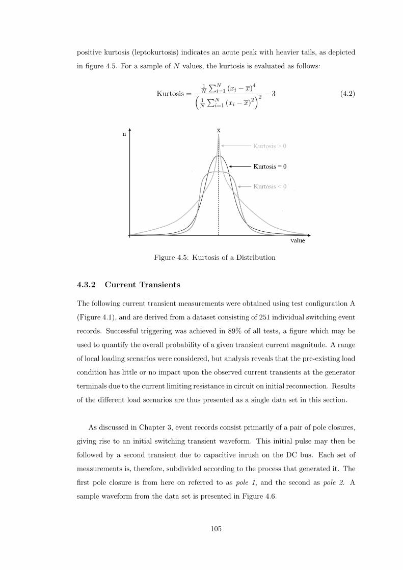
positive kurtosis (leptokurtosis) indicates an acute peak with heavier tails, as depicted

in figure 4.5. For a sample of N values, the kurtosis is evaluated as follows:

Kurtosis =1N

∑Ni=1 (xi − x)4(

1N

∑Ni=1 (xi − x)2

)2 − 3 (4.2)

Figure 4.5: Kurtosis of a Distribution

4.3.2 Current Transients

The following current transient measurements were obtained using test configuration A

(Figure 4.1), and are derived from a dataset consisting of 251 individual switching event

records. Successful triggering was achieved in 89% of all tests, a figure which may be

used to quantify the overall probability of a given transient current magnitude. A range

of local loading scenarios were considered, but analysis reveals that the pre-existing load

condition has little or no impact upon the observed current transients at the generator

terminals due to the current limiting resistance in circuit on initial reconnection. Results

of the different load scenarios are thus presented as a single data set in this section.

As discussed in Chapter 3, event records consist primarily of a pair of pole closures,

giving rise to an initial switching transient waveform. This initial pulse may then be

followed by a second transient due to capacitive inrush on the DC bus. Each set of

measurements is, therefore, subdivided according to the process that generated it. The

first pole closure is from here on referred to as pole 1, and the second as pole 2. A

sample waveform from the data set is presented in Figure 4.6.

105

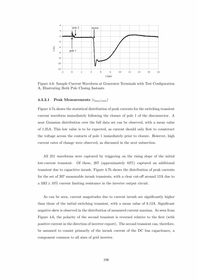
Figure 4.6: Sample Current Waveform at Generator Terminals with Test ConfigurationA, Illustrating Both Pole Closing Instants

4.3.2.1 Peak Measurements (imax/min)

Figure 4.7a shows the statistical distribution of peak currents for the switching transient

current waveform immediately following the closure of pole 1 of the disconnector. A

near Gaussian distribution over the full data set can be observed, with a mean value

of 1.35A. This low value is to be expected, as current should only flow to counteract

the voltage across the contacts of pole 1 immediately prior to closure. However, high

current rates of change were observed, as discussed in the next subsection.

All 251 waveforms were captured by triggering on the rising slope of the initial

low-current transient. Of these, 207 (approximately 82%) captured an additional

transient due to capacitive inrush. Figure 4.7b shows the distribution of peak currents

for the set of 207 measurable inrush transients, with a clear cut-off around 12A due to

a 33Ω± 10% current limiting resistance in the inverter output circuit.

As can be seen, current magnitudes due to current inrush are significantly higher

than those of the initial switching transient, with a mean value of 9.12A. Significant

negative skew is observed in the distribution of measured current maxima. As seen from

Figure 4.6, the polarity of the second transient is reversed relative to the first (with

positive current in the direction of inverter export). The second transient can, therefore,

be assumed to consist primarily of the inrush current of the DC bus capacitance, a

component common to all sizes of grid inverter.

106

(a) Peak Current on Closing Pole 1

(b) Peak Inrush Current

Figure 4.7: Peak Current Distributions

4.3.2.2 Current Rate of Change

(di

dt

)In addition to peak value measurement, it is important to evaluate the rate of change

in the leading and trailing edges of a current waveform. Fast rising current impulses

can accelerate the degradation of insulation, and may cause high voltages to develop

across transformer windings and other inductive network components.

Figures 4.8a and 4.9a depict the statistical distribution of rising and falling edge

rates of change for the initial current transient following pole 1 closing. Due to the

low amplitude of the switching current transient, the presence of even small quantities

of noise can result in errors when determining the 10% rise time. Rising edge rate of

change is thus evaluated over the interval 30% to 90% of the peak value, similar to the

voltage measurement techniques of IEC60 [148], giving a bimodal distribution as seen

in Figure 4.8a. The measured values are split evenly between the two modes; those

of mode 1 occupying the range 20-100 kA/s, with a mean value of 59.4 kA/s, and for

mode 2, a range 100-200 kA/s with a mean of 144.5kA/s.

As can be seen from Figure 4.8b, there is a broadly linear relationship between

the the rate of change and peak current, and the two result clusters giving rise to the

107

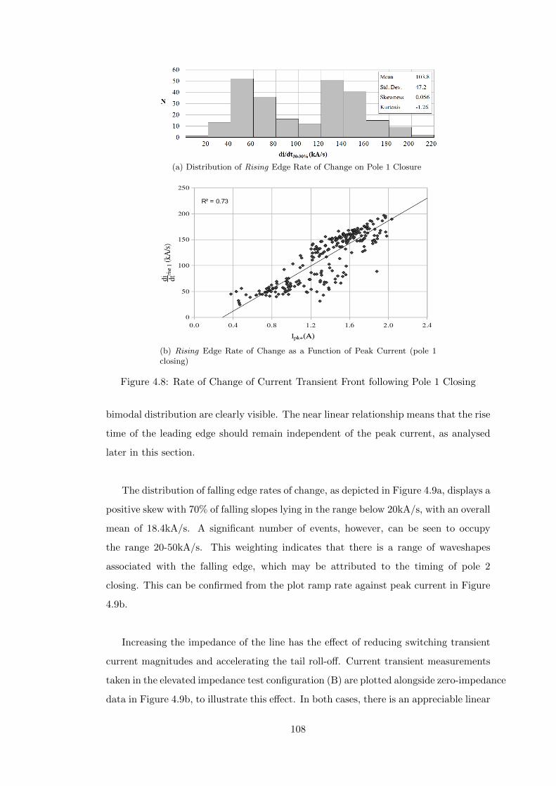
(a) Distribution of Rising Edge Rate of Change on Pole 1 Closure

(b) Rising Edge Rate of Change as a Function of Peak Current (pole 1closing)

Figure 4.8: Rate of Change of Current Transient Front following Pole 1 Closing

bimodal distribution are clearly visible. The near linear relationship means that the rise

time of the leading edge should remain independent of the peak current, as analysed

later in this section.

The distribution of falling edge rates of change, as depicted in Figure 4.9a, displays a

positive skew with 70% of falling slopes lying in the range below 20kA/s, with an overall

mean of 18.4kA/s. A significant number of events, however, can be seen to occupy

the range 20-50kA/s. This weighting indicates that there is a range of waveshapes

associated with the falling edge, which may be attributed to the timing of pole 2

closing. This can be confirmed from the plot ramp rate against peak current in Figure

4.9b.

Increasing the impedance of the line has the effect of reducing switching transient

current magnitudes and accelerating the tail roll-off. Current transient measurements

taken in the elevated impedance test configuration (B) are plotted alongside zero-impedance

data in Figure 4.9b, to illustrate this effect. In both cases, there is an appreciable linear

108

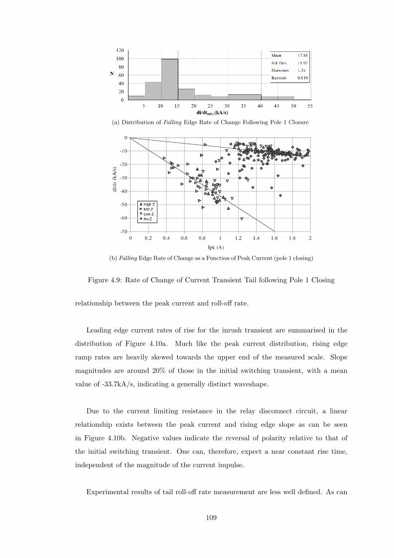
(a) Distribution of Falling Edge Rate of Change Following Pole 1 Closure

(b) Falling Edge Rate of Change as a Function of Peak Current (pole 1 closing)

Figure 4.9: Rate of Change of Current Transient Tail following Pole 1 Closing

relationship between the peak current and roll-off rate.

Leading edge current rates of rise for the inrush transient are summarised in the

distribution of Figure 4.10a. Much like the peak current distribution, rising edge

ramp rates are heavily skewed towards the upper end of the measured scale. Slope

magnitudes are around 20% of those in the initial switching transient, with a mean

value of -33.7kA/s, indicating a generally distinct waveshape.

Due to the current limiting resistance in the relay disconnect circuit, a linear

relationship exists between the peak current and rising edge slope as can be seen

in Figure 4.10b. Negative values indicate the reversal of polarity relative to that of

the initial switching transient. One can, therefore, expect a near constant rise time,

independent of the magnitude of the current impulse.

Experimental results of tail roll-off rate measurement are less well defined. As can

109

(a) Distribution of Inrush Transient Rising Edge Rate of Change

(b) Rising Edge Rate of Change as a Function of Peak Current

(c) Distribution of Inrush Transient Falling Edge Rate of Change

Figure 4.10: Inrush Current Transient: Rising and Falling Edges

be seen from Figure 4.10c, there is a rough bimodal distribution of falling edgedi

dtfrom

peak to half magnitude. This may be partly explained from observation as follows:

1. Inrush initiated during the first quarter cycle of the supply voltage sinusoid results

in a transient in which high current is sustained for the remainder of the half cycle

by the still rising voltage.

2. Pole closure during the second quarter cycle results in a faster rolloff as the voltage

is itself falling away and is unable to sustain the high current.

This effect can be observed in the waveform overlay of Figure 4.11. Case 1 has the

effect of elongating the tail, thus reducing the effective rate of rolloff, while case 2 will

110

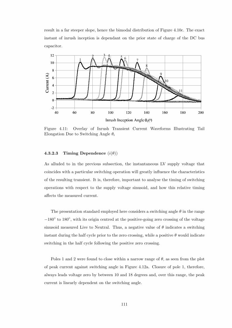
result in a far steeper slope, hence the bimodal distribution of Figure 4.10c. The exact

instant of inrush inception is dependant on the prior state of charge of the DC bus

capacitor.

Figure 4.11: Overlay of Inrush Transient Current Waveforms Illustrating TailElongation Due to Switching Angle θi

4.3.2.3 Timing Dependence (i(θ))

As alluded to in the previous subsection, the instantaneous LV supply voltage that

coincides with a particular switching operation will greatly influence the characteristics

of the resulting transient. It is, therefore, important to analyse the timing of switching

operations with respect to the supply voltage sinusoid, and how this relative timing

affects the measured current.

The presentation standard employed here considers a switching angle θ in the range

−180 to 180, with its origin centred at the positive-going zero crossing of the voltage

sinusoid measured Live to Neutral. Thus, a negative value of θ indicates a switching

instant during the half cycle prior to the zero crossing, while a positive θ would indicate

switching in the half cycle following the positive zero crossing.

Poles 1 and 2 were found to close within a narrow range of θ, as seen from the plot

of peak current against switching angle in Figure 4.12a. Closure of pole 1, therefore,

always leads voltage zero by between 10 and 18 degrees and, over this range, the peak

current is linearly dependent on the switching angle.

111

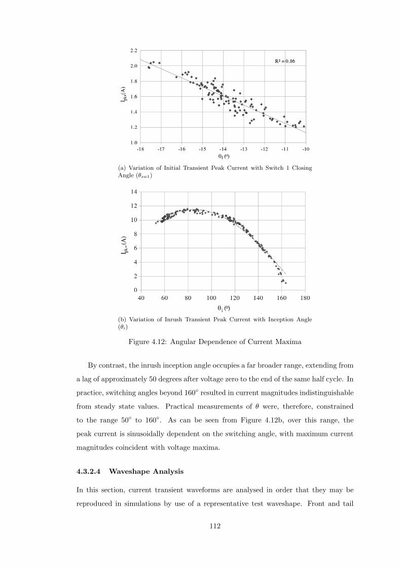
(a) Variation of Initial Transient Peak Current with Switch 1 ClosingAngle (θsw1)

(b) Variation of Inrush Transient Peak Current with Inception Angle(θi)

Figure 4.12: Angular Dependence of Current Maxima

By contrast, the inrush inception angle occupies a far broader range, extending from

a lag of approximately 50 degrees after voltage zero to the end of the same half cycle. In

practice, switching angles beyond 160 resulted in current magnitudes indistinguishable

from steady state values. Practical measurements of θ were, therefore, constrained

to the range 50 to 160. As can be seen from Figure 4.12b, over this range, the

peak current is sinusoidally dependent on the switching angle, with maximum current

magnitudes coincident with voltage maxima.

4.3.2.4 Waveshape Analysis

In this section, current transient waveforms are analysed in order that they may be

reproduced in simulations by use of a representative test waveshape. Front and tail

112

times are compared with the ranges defined in Insulation Coordination Standards

[120,138,142] for the purpose of classification.

Figure 4.14a shows the distribution of measured rise times for all captured switching

current transients. The total rise time T1 is linearly extrapolated from T30−90% by

multiplying by the factor 1.67 as defined in [148] for voltage measurements. The mean

rise time of Figure 4.14a is approximately 15.4µs.

The tail times T2 of the initial switching current transient are depicted in Figure

4.14b, as measured from the extrapolated switching instant to the 50% roll-off point

as shown in figure 4.13. The mean tail time was found to be 80.9µs, meaning that the

average switching current transient falls within the definition of a fast-front according

to BS EN 60071-1 [138].

Figure 4.13: Evaluation of T1 and T2 as per [138]

An equivalent analysis has been performed for the inrush transient, with rise time

distributions plotted in Figure 4.14c, and tail distributions in Figure 4.14d. Average and

extreme values of the waveshape components are summarised in Table 4.4, and are used

in the specification of a representative double exponential pulse for later simulations as

per [120].

113

(a) Pole 1 Switching Transient Front Rise Time (T1)

(b) Pole 1 Switching Transient Tail Times (T2)

(c) Inrush Current Transient Rise Time (T1)

(d) Inrush Current Transient Tail Time (T2)

Figure 4.14: Current Transient Waveshape Components

114

Table 4.4: Summary of Transient Current Waveshape Components

Switching Transient Ipk1 (A) T1 (µs) T2 (µs)

Mean Value 1.34 15.5 80.9Minimum 0.38 8.5 22.9Maximum 2.05 41.5 224.5

Inrush Transient Ipk2 (A) T1 (µs) T2 (µs)

Mean Value 9.12 270.8 2,630Minimum 0.46 243 785Maximum 11.6 705 5,366

4.3.3 Voltage Transients

Voltage transient measurements were obtained from a set of 120 event records using

laboratory test configuration B (see Figure 4.2). The transients were isolated for

analysis by subtraction of the mains voltage sinusoid, leaving a waveform consisting

solely of voltage impulses and supply harmonics. This method introduces the potential

for error in time-zeroing the sinusoid, and a voltage offset may occur. Absolute magnitudes

may, therefore, deviate by up to 5V either side of the true value.

4.3.3.1 Peak Measurements (vmax, vmin)

Peak voltages obtained without the series line impedance compensation (Zmin = 0.12Ω)

were generally too small to distinguish from background noise and supply harmonics

(see Figure 4.2). The results presented here are those obtained with an elevated series

impedance. From the data obtained, it is observed that an increase in series impedance

beyond 0.4Ω at 50Hz has little determinable effect on voltage distortion, and Figure

4.15a illustrates the combined distribution of positive voltage peaks for low- mid- and

high-impedance cases. It is possible that a larger data set would begin to illustrate

some trend, but it would be inconclusive to infer such a relationship from this small

data set.

Figure 4.15a gives a mean pole 1 switching transient voltage magnitude of 47.5V,

at a standard deviation of 12.9V. Figure 4.15b indicates a broadly linear relationship

between switching voltage and current transient magnitudes for the elevated line impedance

scenario. Error bars of ±5V are included.

115

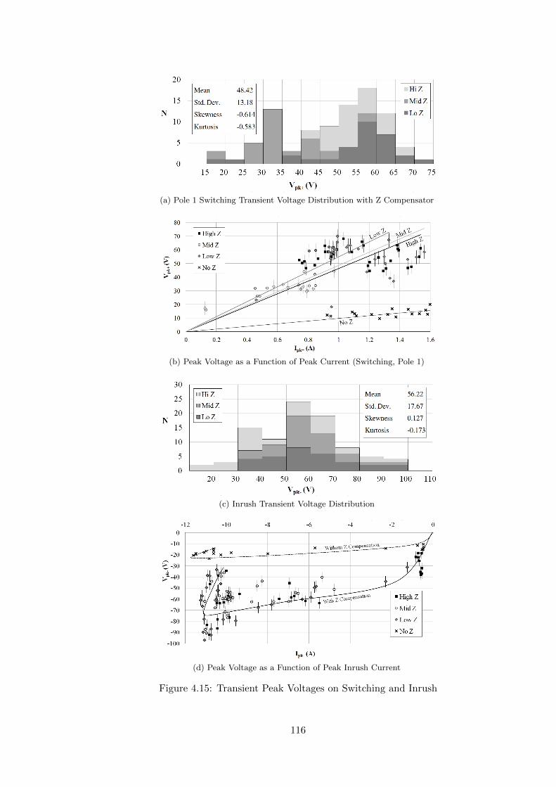
(a) Pole 1 Switching Transient Voltage Distribution with Z Compensator

(b) Peak Voltage as a Function of Peak Current (Switching, Pole 1)

(c) Inrush Transient Voltage Distribution

(d) Peak Voltage as a Function of Peak Inrush Current

Figure 4.15: Transient Peak Voltages on Switching and Inrush

116

Of the 91 switching waveforms captured under the increased line impedance scenario,

82 (90%) recorded a second additional transient due to current inrush. Inrush transient

magnitudes were similarly unaltered by change in supply impedance, and are presented

cumulatively in Figure 4.15c. Mean voltage magnitude is 55.7V, with a standard

deviation of 17.6V.

A relationship between inrush peak voltages and currents is somewhat more pronounced

than with the switching transients, as can be seen from Figure 4.15d (negative values

indicating a reversal of polarity with respect to switching transient measurements).

Due to a distinct weighting of results towards the upper end of the current scale, it is

difficult to derive a singular relationship over the full current range. There is, however,

a visible divergence of peak voltage with increasing current suggesting a two-slope or

polynomial relationship.

As discussed in section 4.3.2, the rising edge rate of change of the inrush current

transient varies linearly with current magnitude. For a low voltage feeder with series

resistance R and reactance X, the voltage drop should be a function of both the current

and its derivative, with the effect ofdi

dtdominating for very steep rising edges. This

explains the nonlinear slope of Figure 4.15d.

4.3.3.2 Voltage Rate of Change

(dv

dt

)As with the current transients of section 4.3.2, voltage waveforms were analysed to

determine rising and falling edge rates of change. General observation indicates that

leading and trailing edges are nearly symmetrical, as distinct from the fast rise and

relatively slow tail of the current waveforms. Voltage rates of change are, therefore,

evaluated over the intervals 30%-90% and 90%-30% of peak for the front and tail

respectively.

Figures 4.16a and 4.16b show the distributions of rising and falling edge voltage

ramp rates respectively. Similarly, Figures 4.16c and 4.16d are the distributions of

inrush rising and falling edge ramp rates. A statistical analysis of these datasets is

summarised in Table 4.5.

117

(a) Pole 1 Switching Transient Transient Rising Edgedv+

dt

(b) Pole 1 Switching Transient Falling Edgedv−dt

(c) Inrush Transient Rising Edgedv+

dt

(d) Inrush Transient Falling Edgedv−dt

Figure 4.16: Voltage Transient Rate of Change Statistics

118

Table 4.5: Statistical Variation of Measured Voltage Rates of Change

Quantity Switching ↑ Switching ↓ Inrush ↑ Inrush ↓

v 3170 kV/s -2754 kV/s -343 kV/s 283 kV/sσ 1254 kV/s 2037 kV/s 90 kV/s 101 kV/s

4.3.3.3 Waveshape Analysis

Given the similarity of rising and falling edge rates of change for both switching and

inrush voltage transients, a typical waveform may be expected to display a good

degree of symmetry about its peak. Thus, little similarity exists between the measured

waveforms and either of the standard insulation coordination test waveshapes as presented

in Chapter 3. Arbitrarily treating the measured waveforms as fast-front impulses as in

[138], the front and tail times (T1, T2) have been calculated as per Figure 4.13 and are

summarised in Figures 4.17a to 4.17d.

Switching transient front times form a neat Gaussian distribution about a mean

value of 15.8µs as shown in Figure 4.17a, while the tail times of Figure 4.17b, as

measured from the virtual zero of the rising edge to the 50% decay point, are considerably

more dispersed. A significant weighting of results in the region 10 to 30 µs keeps the

mean value low at 32.3µs, but the numerous outlying results between 30 and 85µs

should not be ignored.

Front and Tail times for the inrush voltage transient form a somewhat neater pair

of distributions, as can be seen from Figures 4.17c and 4.17d. Mean values of 191.5 and

299.3 µs were recorded for T1 and T2 respectively. Statistical analyses are summarised

in Table 4.6.

Table 4.6: Statistical Variation of Measured Voltage Front and Tail Times

Quantity Switching Transient Inrush Transient

T1 15.8 µs 191.5 µsσ 9.8 µs 132.6 µs

T2 32.3 µs 299.3 µsσ 26.6 µs 160.1 µs

119

(a) Distribution of Switching Transient Front Times (T1)

(b) Distribution of Switching Transient Tail Times (T2)

(c) Distribution of Inrush Transient Front Times (T1)

(d) Distribution of Inrush Transient Tail Times (T2)

Figure 4.17: Voltage Transient Waveshape Components

120

4.3.4 Switch Timing

One of the most important factors to consider in the development of the simulation

models is the timing of transient fronts relative to the supply voltage sinusoid, and thus

the delay between the closing instants of poles 1 and 2 and instant of inrush inception.

Statistical switching analyses using EMTP-ATP require that the distribution in time

of pole closure times be known, while a master-slave switch implementation requires

an evaluation of the pole delay statistics.

For the purpose of the following analyses, the full set of 251 current transient

waveforms from section 4.3.2 have been used as they have more clearly defined switching

times than the equivalent set of voltage transients. Pole closing angles are determined

by identifying absolute switching times from a current waveform, then indexing the

associated voltage sinusoid.

4.3.4.1 Pole Angle (θsw)

Figure 4.18a gives the distribution of pole 1 closing angles. As noted earlier in this

chapter, the first pole closure leads the positive-going voltage zero and is confined to a

relatively narrow range of values between 6 and 20. The distribution itself is clearly

Gaussian, with a mean value of 13.8, making the statistical switch the ideal choice for

simulation of the leading pole closure.

4.3.4.2 Switch / Inrush Delay (τsw, τi)

Figure 4.18b depicts the distribution of switching delays between poles 1 and 2 of the

generator disconnect. The delay between closure of the first disconnector pole and the

subsequent current inrush is shown in Figure 4.18c. While the switching delay τsw

occupies a broadly Gaussian distribution, that of the inrush delay τi is comparatively

flat (negative kurtosis). In the absence of additional statistical data, a continuous

uniform distribution of τi over the range 3.5 to 10 ms has been chosen for the purpose

of implementing statistical switches (see Chapter 6).

4.3.5 Transient Energy

The final quantity of interest is a measure of the energy content of the transient. This

gives an indication of the duty requirements of equipment in the vicinity of the switch,

121

(a) Distribution of Pole 1 Switching Angles Leading Voltage Zero

(b) Distribution of Switching Delay τsw

(c) Distribution of Inrush Inception Delay τi

Figure 4.18: Switching Angles and Delay Times

122

but also completes a set of measurable quantities from which equivalent EMC test

waveforms may be calculated.

4.3.5.1 Current Transient Energy Measure (Si)

Current transient energy measures are computed from the set of waveforms used in

section 4.3.2, for both switching and inrush transients where applicable. The energy

measure Si was evaluated by trapezoidal integration using (4.3).

Si =

∫ T

t=0i2(t)dt (4.3)

The resulting values are plotted in Figures 4.19a and 4.19b as functions of the

switching angle θ. Over the narrow range occupied by θ1, the energy measure is roughly

linearly dependent on the switching angle, much like the peak current and ramp rate.

Inrush inception by contrast may occur at almost any instant in half cycle following

the positive-going zero crossing of the voltage sinusoid.

As discussed in section 4.3.2, the tail time of a given inrush current transient is

heavily dependent on the inrush inception angle, with high sustained currents occurring

in the range θi < 90. The energy measure is proportional to the integral of a sinusoid

between θi and 180. The overlay in Figure 4.19b is a plot of this integral, with an

additional scaling factor of 0.44.

4.3.5.2 Voltage Transient Energy Measure (Sv)

Measurements of the voltage transient energy measure Sv were similarly performed on

the result set of section 4.3.3. As discussed earlier, amplitude measurements on this

data set are subject to a potential systematic offset error due to subtraction of the

voltage sinusoid during the preprocessing stage. This error is unavoidably amplified

in the calculation of Sv due to the squaring of measured values. Taking as before the

conservative offset error in voltage measurements as ± 5V , then for a mean switching

transient voltage peak of 47.5V, the error margin in Sv becomes ±22%. This is reduced

to ±18% for the inrush transient due to the increased mean voltage peak of 55.7V.

Figures 4.20a and 4.20b illustrate the relationship between Sv and θ for the switching

and inrush transients respectively. Much like the current energy measure, Sv1 for the

123

(a) Pole 1 Switching Transient Si as Function of θ1

(b) Inrush Transient Si as Function of θi

Figure 4.19: Current Transient Energy Measures as Functions of θ

124

switching transient is broadly linearly dependent on the pole angle θ1, over the measured

range.

Sv2 by contrast is roughly proportional to sin2(θ2), as can be seen from the curve

overlay in Figure 4.20b, with peak energy measure of approximately 1.5V 2s occurring

at θ2 ≈ 90.

(a) Pole 1 Switching Transient Sv as Function of θ1

(b) Inrush Transient Sv as Function of θi

Figure 4.20: Voltage Transient Energy Measures as Functions of θ

4.3.5.3 Waveform Energy Content (W )

In addition to the voltage and current waveforms pairs output by the transient logger,

a third waveform was constructed by multiplication of the instantaneous values of both

measured quantities. The energy content of the transients can, therefore, be estimated

by integration of the waveform product v(t) · i(t) over the pulse duration. The data set

of section 4.3.2 was once again used for the calculation of energy content.

W1, the energy content of the switching transients, is presented as a distribution in

Figure 4.21a. As expected from the short duration and low magnitude of the switching

125

current transient, and its proximity to the voltage zero crossing, the energy content is

very low, with a mean value of 8.2mJ . The plot of Figure 4.21b illustrates the linear

dependence of W1 on the pole angle θ1.

Of greater interest is the energy content of the inrush transient W2. As can be seen

from Figure 4.21c, typical values of W2 are around three orders of magnitude larger

than those of the switching transient, with a mean value of 5.2J . This is due to the

increased current magnitudes and slower front and tail times of the inrush transient.

As with the current energy measure Si2, the energy content W2 is proportional to the

integral of sin θ2, as shown by the overlay in Figure 4.21d. The theoretical maximum

value of the curve fitting is 15.5J, but in practice no switching angles smaller than 50

were observed during testing regime, effectively limiting W2 for this particular device

to approximately 13.6J .

4.4 Standardised Test Waveform Components

This section summarises the computation of a selection of standard test waveform

components from experimental quantities, as introduced in Chapter 3. This will assist

in the modelling of observed phenomena as presented in Chapters 5 and 6. The section

is split according to the type of standard employed, and a discussion of calculation

methods included in each subsection.

4.4.1 Insulation Coordination

The standard test waveshapes of BS EN 60071-1 [138] for systems rated above 100V

are summarised in Figure 4.22. Insulation Coordination standards for systems rated

below 1000V (BS EN 60664 [137]) make reference to standard impulse test waveforms,

but provide little assistance with regard to waveshape specifications.

4.4.1.1 Slow-Front Transient

Of the data sets analysed in this chapter, only the current inrush transient falls within

the definition of a slow-front waveshape. Table 4.7 summarises the typical and worst-case

shape factors for the purpose of repeat simulations.

126

(a) Distribution of Switching Transient Energy Content (W1)

(b) Switching Transient Energy Content as Function of θ1

(c) Distribution of Inrush Transient Energy Content (W2)

(d) Inrush Transient Energy Content as Function of θi

Figure 4.21: Waveform Energy Content (W)

127

(a) Slow-Front (b) Fast-Front

Figure 4.22: Standard Waveshapes of BS EN 60071

Table 4.7: Slow-Front Waveform Components of Inrush Current Transient

I2 pk (A) Tp (µs) T2 (ms)

∆I2Typical 9 300 2.5

Worst Case 12 250 5.5

4.4.1.2 Fast-Front Transient

The remaining data sets fall between the definitions of slow- and fast-front transients,

and only the switching current impulse displays a classically large ratio of front and

tail times. Voltage transients (switching and inrush) were found to exhibit a high

degree of symmetry about the peak, lending themselves more readily to representation

as symmetrical trapezoidal pulses. Table 4.8 summarises the typical and worst-case

values of the fast-front waveshape components for the remaining measured data sets.

Table 4.8: Fast-Front Waveform Components of Measured Transients

Peak Value T1 (µs) T2 (µs)

∆I1Typical 1.5 A 15 80

Worst Case 2 A 8 225

∆V1Typical 50 V 16 32

Worst Case 70 V 8 80

∆V2Typical 60 V 200 300

Worst Case 100 V 100 450

4.4.2 Electromagnetic Compatibility

A selection of typical Electromagnetic Compatibility test waveshapes, as used for the

classification of low-voltage transients in [81] are presented in Figure 4.23. These

waveshapes offer an alternative method for the application of experimental data to

simulation, as have been chosen as their components can be easily evaluated from

128

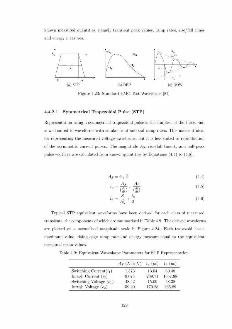
known measured quantities; namely transient peak values, ramp rates, rise/fall times

and energy measures.

(a) STP (b) DEP (c) DOW

Figure 4.23: Standard EMC Test Waveforms [81]

4.4.2.1 Symmetrical Trapezoidal Pulse (STP)

Representation using a symmetrical trapezoidal pulse is the simplest of the three, and

is well suited to waveforms with similar front and tail ramp rates. This makes it ideal

for representing the measured voltage waveforms, but it is less suited to reproduction

of the asymmetric current pulses. The magnitude AS , rise/fall time ta and half-peak

pulse width th are calculated from known quantities by Equations (4.4) to (4.6).

AS = v , i (4.4)

ta =AS

(dvdt ),As

(didt)(4.5)

th =S

A2S

+ta3

(4.6)

Typical STP equivalent waveforms have been derived for each class of measured

transients, the components of which are summarised in Table 4.9. The derived waveforms

are plotted on a normalised magnitude scale in Figure 4.24. Each trapezoid has a

maximum value, rising edge ramp rate and energy measure equal to the equivalent

measured mean values.

Table 4.9: Equivalent Waveshape Parameters for STP Representation

AS (A or V) ta (µs) th (µs)

Switching Current(i1) 1.573 13.04 60.48Inrush Current (i2) 9.074 289.71 1657.98Switching Voltage (v1) 48.42 15.09 48.38Inrush Voltage (v2) 59.20 179.28 265.89

129

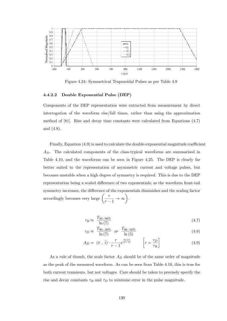
Figure 4.24: Symmetrical Trapezoidal Pulses as per Table 4.9

4.4.2.2 Double Exponential Pulse (DEP)

Components of the DEP representation were extracted from measurement by direct

interrogation of the waveform rise/fall times, rather than using the approximation

method of [81]. Rise and decay time constants were calculated from Equations (4.7)

and (4.8).

Finally, Equation (4.9) is used to calculate the double-exponential magnitude coefficient

AD. The calculated components of the class-typical waveforms are summarised in

Table 4.10, and the waveforms can be seen in Figure 4.25. The DEP is clearly far

better suited to the representation of asymmetric current and voltage pulses, but

becomes unstable when a high degree of symmetry is required. This is due to the DEP

representation being a scaled difference of two exponentials; as the waveform front-tail

symmetry increases, the difference of the exponentials diminishes and the scaling factor

accordingly becomes very large

(r

r − 1→∞

).

τR ≈T30−90%

ln (7)(4.7)

τD ≈T90−30%

ln (7)or

T90−50%

ln (5)(4.8)

AD = (v , i) · r

r − 1e

ln (r)(r−1)

[r =

τDτR

](4.9)

As a rule of thumb, the scale factor AD should be of the same order of magnitude

as the peak of the measured waveform. As can be seen from Table 4.10, this is true for

both current transients, but not voltages. Care should be taken to precisely specify the

rise and decay constants τR and τD to minimise error in the pulse magnitude.

130

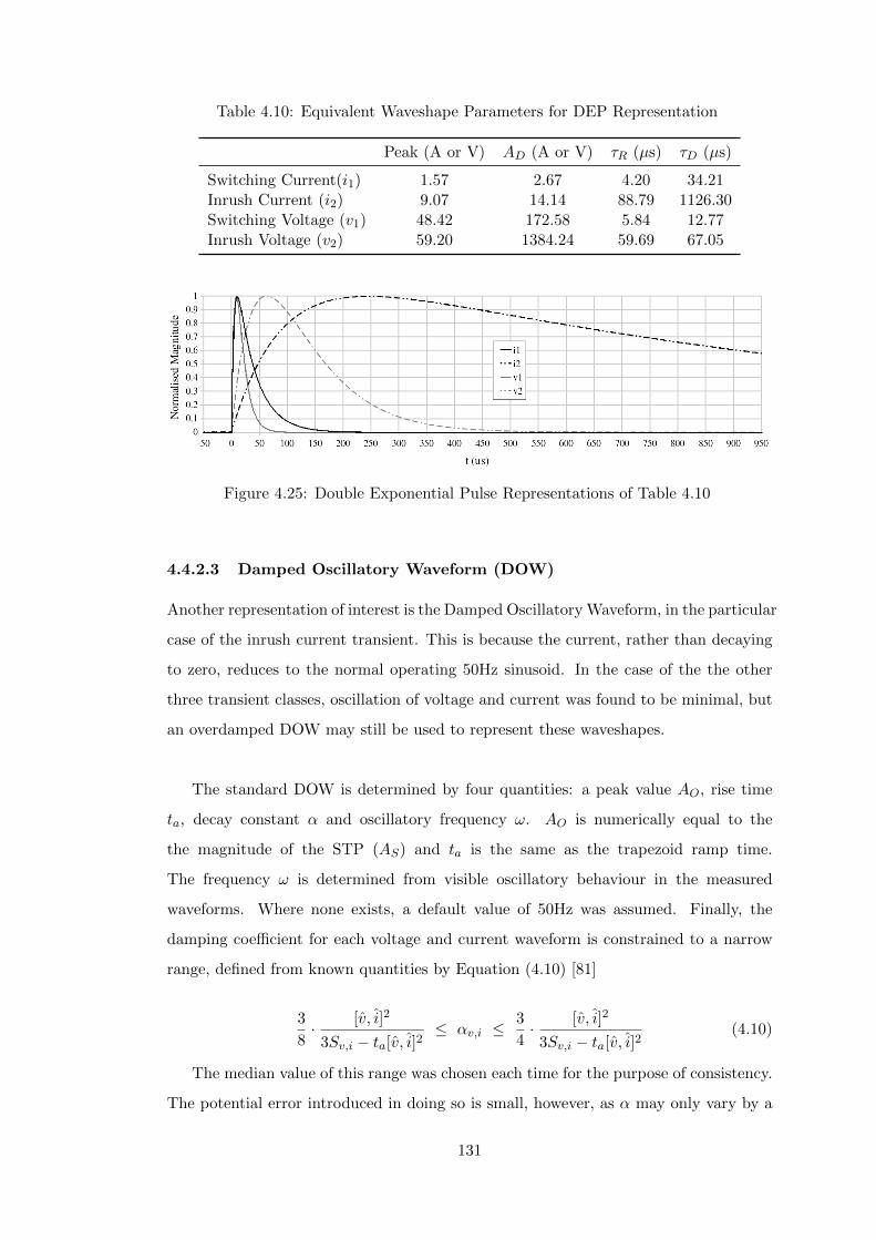
Table 4.10: Equivalent Waveshape Parameters for DEP Representation

Peak (A or V) AD (A or V) τR (µs) τD (µs)

Switching Current(i1) 1.57 2.67 4.20 34.21Inrush Current (i2) 9.07 14.14 88.79 1126.30Switching Voltage (v1) 48.42 172.58 5.84 12.77Inrush Voltage (v2) 59.20 1384.24 59.69 67.05

Figure 4.25: Double Exponential Pulse Representations of Table 4.10

4.4.2.3 Damped Oscillatory Waveform (DOW)

Another representation of interest is the Damped Oscillatory Waveform, in the particular

case of the inrush current transient. This is because the current, rather than decaying

to zero, reduces to the normal operating 50Hz sinusoid. In the case of the the other

three transient classes, oscillation of voltage and current was found to be minimal, but

an overdamped DOW may still be used to represent these waveshapes.

The standard DOW is determined by four quantities: a peak value AO, rise time

ta, decay constant α and oscillatory frequency ω. AO is numerically equal to the

the magnitude of the STP (AS) and ta is the same as the trapezoid ramp time.

The frequency ω is determined from visible oscillatory behaviour in the measured

waveforms. Where none exists, a default value of 50Hz was assumed. Finally, the

damping coefficient for each voltage and current waveform is constrained to a narrow

range, defined from known quantities by Equation (4.10) [81]

3

8· [v, i]2

3Sv,i − ta[v, i]2≤ αv,i ≤

3

4· [v, i]2

3Sv,i − ta[v, i]2(4.10)

The median value of this range was chosen each time for the purpose of consistency.

The potential error introduced in doing so is small, however, as α may only vary by a

131

factor of 2 over its full range. Table 4.11 summarises the calculated shape factors for

the four measured transient classes.

Table 4.11: Equivalent Waveshape Parameters for DOW Representation

AO (A or V) ta (µs) α (kHz) ω (Hz)

Switching Current(i1) 1.57 13.04 6.914 ∼1000Inrush Current (i2) 9.07 289.71 0.47 ∼70

Switching Voltage (v1) 48.42 15.09 18.88 ∼2000Inrush Voltage (v2) 59.20 179.30 3.94 ∼1200

Representative damped oscillatory waveforms are depicted in Figure 4.26 for both

switching and inrush current and voltage transients. Typical waveforms captured with

the transient logger are overlaid for reference. As can be seen from these plots, the DOW

is particularly suited to the representation of slow-front inrush current transients, where

sinusoidal behaviour follows the tail roll-off. For fast-front transients, however, the

coefficient α is large enough to result in critical damping. In this case, the frequency

ω simply becomes a shape factor that can be used to fit the exponential curve to

the tail. In this mode of operation, there is little to distinguish the DOW from the

double-exponential, except that the rising edge is here assumed to be linear over the

rise time ta.

4.4.3 Suitability of Waveshapes

From the analysis of measured waveshape components T1 and T2, it is noted that

established insulation coordination test waveforms for slow- and fast-front transients do

not necessarily give the best reproduction of measured phenomena. With the exception

of the inrush current transient (∆I2), all measured characteristics fall somewhere between

the standard definitions of slow-front and fast-front transients, and in the case of

voltage transients (∆V ) there is a greater degree of symmetry between the front and

tail than is allowed by the standard 1.2/50µs lightning impulse. Measured switching

voltage transients (∆V1) might be better represented using the standard 8/20µs surge

waveshape of BS EN 61000 [149], more commonly used for current injection tests.

The use of more arbitrarily defined EMC waveshapes (STP,DEP and DOW) gives

more flexibility to reproduce specific transient characteristics, as each of these shapes

132

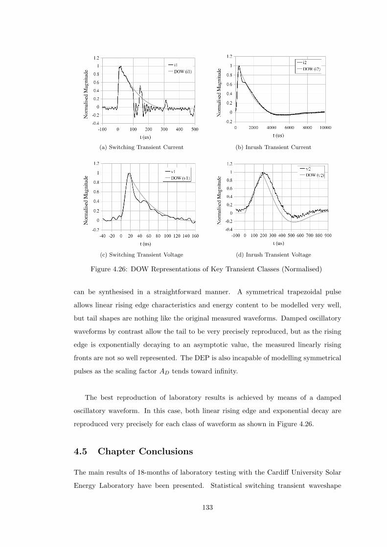
(a) Switching Transient Current (b) Inrush Transient Current

(c) Switching Transient Voltage (d) Inrush Transient Voltage

Figure 4.26: DOW Representations of Key Transient Classes (Normalised)

can be synthesised in a straightforward manner. A symmetrical trapezoidal pulse

allows linear rising edge characteristics and energy content to be modelled very well,

but tail shapes are nothing like the original measured waveforms. Damped oscillatory

waveforms by contrast allow the tail to be very precisely reproduced, but as the rising

edge is exponentially decaying to an asymptotic value, the measured linearly rising

fronts are not so well represented. The DEP is also incapable of modelling symmetrical

pulses as the scaling factor AD tends toward infinity.

The best reproduction of laboratory results is achieved by means of a damped

oscillatory waveform. In this case, both linear rising edge and exponential decay are

reproduced very precisely for each class of waveform as shown in Figure 4.26.


The main results of 18-months of laboratory testing with the Cardiff University Solar

Energy Laboratory have been presented. Statistical switching transient waveshape

133

datasets for voltage and current magnitudes, ramp rates and energy measures have

been acquired for 251 unique event records. Analysis of switching angles has been used

to determine the relative timing of pole closing and inverter capacitive inrush inception,

for the purpose of translation to statistically determined switching models in EMTP.

The main conclusions are as follows:

• Generator disconnection under export conditions produces no measurable transient

voltages due to current interruption occurring at V ≈ 0V in a predominantly

resistive circuit.

• Reconnection operations involve the closing of a pair of relay poles at the zero-crossing

of the supply voltage sinusoid, with a mean pole separation of 0.7ms.

• Relay pole closing gives rise to an initial fast front, low magnitude current transient

(typical: 1.5A, 15/80µs)

• In approximately 80% of cases, switching is followed by a slow-front, higher

magnitude inrush current transient (9A, 300/2500µs) associated with charging

of the inverter DC bus capacitance. Mean inrush delay time was found to be

approximately 9.4ms.

• A transient voltage perturbation is associated with each current transient, its

magnitude dependent on the current amplitude and impedance of the incoming

mains supply (switching: 16/32µs, inrush: 200/300µs)

• Measured transient characteristics may be reproduced using a variety of synthesisable

test waveshapes common to insulation coordination and EMC standards. It was

found that a damped oscillatory waveform representation gives the best overall

reproduction of front and tail characteristics, and has the flexibility to handle

each class of measured voltage and current waveshape.

134

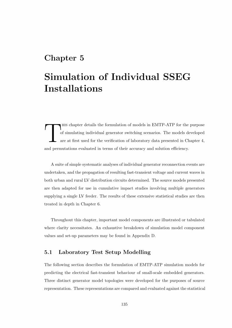
Chapter 5

Simulation of Individual SSEGInstallations

This chapter details the formulation of models in EMTP-ATP for the purpose

of simulating individual generator switching scenarios. The models developed

are at first used for the verification of laboratory data presented in Chapter 4,

and permutations evaluated in terms of their accuracy and solution efficiency.

A suite of simple systematic analyses of individual generator reconnection events are

undertaken, and the propagation of resulting fast-transient voltage and current waves in

both urban and rural LV distribution circuits determined. The source models presented

are then adapted for use in cumulative impact studies involving multiple generators

supplying a single LV feeder. The results of these extensive statistical studies are then

treated in depth in Chapter 6.

Throughout this chapter, important model components are illustrated or tabulated

where clarity necessitates. An exhaustive breakdown of simulation model component

values and set-up parameters may be found in Appendix D.

5.1 Laboratory Test Setup Modelling

The following section describes the formulation of EMTP-ATP simulation models for

predicting the electrical fast-transient behaviour of small-scale embedded generators.

Three distinct generator model topologies were developed for the purposes of source

representation. These representations are compared and evaluated against the statistical

135

data generated from the laboratory tests of Chapter 4. The applicability of the developed

topologies to up-scaling for large multi-source simulations is discussed with reference

to solution efficiency and software capability.

5.1.1 Full Inverter Model

The most elaborate of the three topologies explicitly represents all electrical components

of inverter and primary source, as illustrated in Figure 5.1. In this instance, a 640W

rated photovoltaic array was chosen in line with the laboratory specification. An

interchangeable lower capacity source was also specified according to the measured

VI characteristic of the array.

Figure 5.1: Full Inverter Model Schematic

A nonlinear current source was employed for representation of the PV array, similar

to that proposed in [150]. The nonlinear source is implemented as a current generator

in parallel with a diode defined by a 20-point piecewise linear approximation of the

Shockley equation. The current source is fixed at the nominal short-circuit current

of the array, and the diode V-I curve defined such that the full source current is

circulated when VD equals the open circuit voltage of the array. The diode characteristic

knee-point is defined according to the nominal maximum power point (MPP). These

quantities are summarised in Table 5.1 for both the full rating of the array and its

measured performance.

Table 5.1: Nominal Design Values for PV Array Current-Source Model [145]

Quant. Nominal Measured Equivalent Cct Representation (figure 5.2)

Isc 4.8A 4.64A Current Source Value (IDC)Voc 164V 151.1V Diode Voltage (VD) when ID = IscImpp 4.55A 2.83A Difference Current Isc − ID when VD = VmppVmpp 138.4V 123.3V Diode Voltage VD when ID = Isc − Impp

136

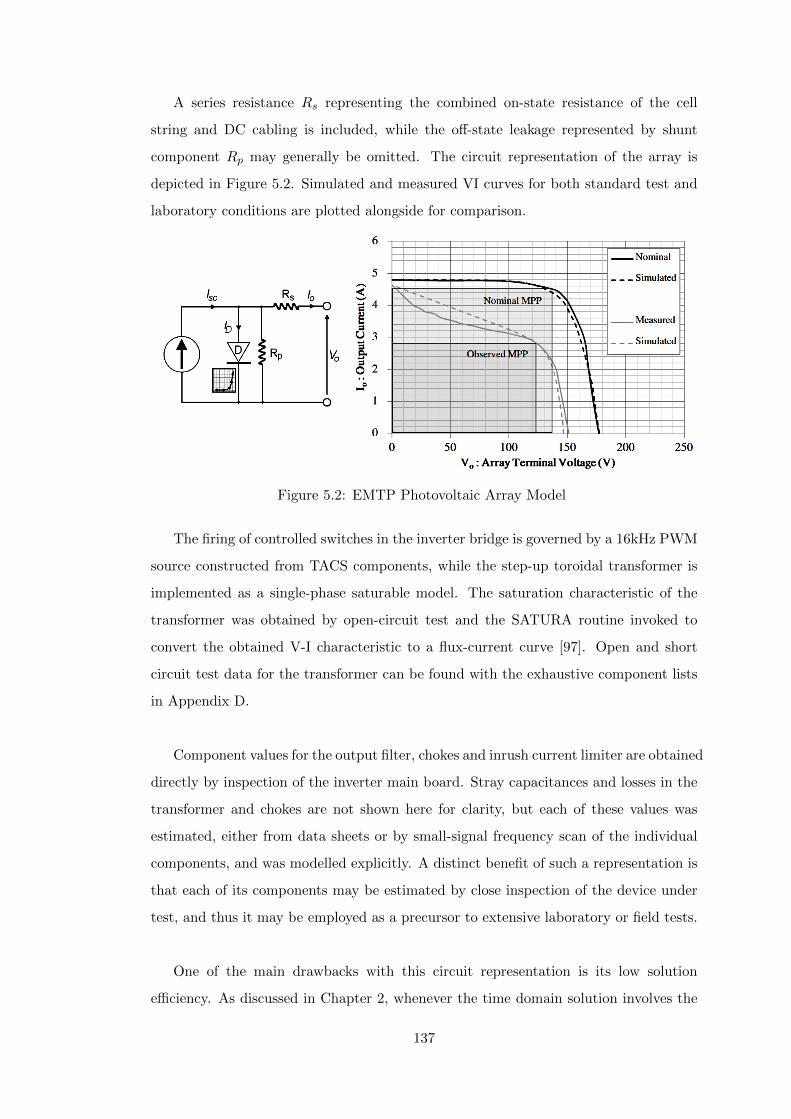
A series resistance Rs representing the combined on-state resistance of the cell

string and DC cabling is included, while the off-state leakage represented by shunt

component Rp may generally be omitted. The circuit representation of the array is

depicted in Figure 5.2. Simulated and measured VI curves for both standard test and

laboratory conditions are plotted alongside for comparison.

Figure 5.2: EMTP Photovoltaic Array Model

The firing of controlled switches in the inverter bridge is governed by a 16kHz PWM

source constructed from TACS components, while the step-up toroidal transformer is

implemented as a single-phase saturable model. The saturation characteristic of the

transformer was obtained by open-circuit test and the SATURA routine invoked to

convert the obtained V-I characteristic to a flux-current curve [97]. Open and short

circuit test data for the transformer can be found with the exhaustive component lists

in Appendix D.

Component values for the output filter, chokes and inrush current limiter are obtained

directly by inspection of the inverter main board. Stray capacitances and losses in the

transformer and chokes are not shown here for clarity, but each of these values was

estimated, either from data sheets or by small-signal frequency scan of the individual

components, and was modelled explicitly. A distinct benefit of such a representation is

that each of its components may be estimated by close inspection of the device under

test, and thus it may be employed as a precursor to extensive laboratory or field tests.

One of the main drawbacks with this circuit representation is its low solution

efficiency. As discussed in Chapter 2, whenever the time domain solution involves the

137

opening or closing of a switch, partial re-triangularisation of the circuit admittance

matrix must be performed before the solver can proceed. Simulation of a 16kHz

PWM bridge such as that depicted in Figure 5.1 requires a minimum of 640 such

operations per power frequency cycle (assuming that all four poles switch on the same

time step), constituting a significant portion of the overall solution time. Every effort

must, therefore, be made to minimise the extent of the solution time window.

A constraint was placed on the time taken for the circuit to settle into its steady

state, prior to executing the switching operation of interest. Using such a brute-force

approach, the settling time demanded by full emulation of the inverter control logic was

found to be prohibitively long. Modelling of the controller has accordingly been omitted

from this model, but as a consequence the initial state of the inverter (principally, the

DC bus voltage and array output current) must be manually specified. While this is

minor concern for simulations involving individual cases, translation of such a model

for the purpose of statistical study, or for cumulative impact assessments of generator

sets across multiple phases, quickly becomes cumbersome. For very large simulations,

there is the added problem of potential branch and node limit violation. This aspect

is covered in more detail in section 5.1.7.

5.1.2 Idealised AC Source Model

A generator disconnect operation may be represented somewhat more simply by replacing

the inverter bridge and its associated firing circuit with an equivalent AC source and

impedance, as depicted in Figure 5.3. This topology eliminates the most computationally

inefficient component of its predecessor, namely the high-frequency switching in the

bridge circuit, while preserving the type-98 piecewise pseudo-nonlinear inductance for

transformer saturation.

Of the three source variants presented, it is the simplified AC model that bears

greatest resemblance to that employed during the early stages of research [151, 152].

Numerous refinements have since been made in the light of laboratory tests to improve

the flexibility of the model. These relate principally to the inclusion of inverter inrush

currents such that the AC source model may also be used to model generator reconnection.

Transformer inrush is handled by means of a single-phase nonlinear transformer

138

Figure 5.3: Reduced AC Source Model Schematic

model, taken directly from the PWM inverter circuit of 5.1.1. In the absence of the

inverter bridge, the capacitive component of the inrush current is initially absent.

On closing the generator output breakers, the inverter DC bus capacitor is charged

from the grid [153], the bypass diodes of the off-state power-electronic switches acting

as a bridge rectifier as depicted in Figure 5.4a. As was noted in Chapter 4, the inrush

duration is generally very short, and the instantaneous current magnitude drops to

less than 1A within 10ms of inception. This behaviour may be simply represented by

means of a pair of series connected capacitors as shown in Figure 5.4b, with an inrush

capacitance Ci many times larger than the initially bypassed steady-state capacitor Cs.

With the aid of measured current waveforms for calibration purposes, the capacitive

inrush is artificially restored by adding this branch on the source side of the transformer

as depicted in Figure 5.3.

(a) DC capacitor charging in off-state (b) Artificial Inrush Circuit

Figure 5.4: Capacitive Inrush Mechanism and Modelling

For the remainder of the positive half cycle following closure of the inrush switch

139

swi, Cs is bypassed by the diode allowing a large charging current to flow. After the first

negative-going voltage zero, the diode becomes reverse biased and the current reduced

accordingly. For simulation cases spanning multiple 50Hz cycles, repeated fictitious

capacitive inrush is prevented by opening the cut-out switch swco prior to the next

positive-going voltage zero. A delay of 10ms between closing swi and opening swco is

sufficient for this purpose. A typical switch timing arrangement is illustrated in Figure

5.5 with reference to the terminal voltage sinusoid.

Figure 5.5: Switch Timing for Capacitive Inrush Circuit

5.1.3 Capacitive Inrush Model

Further reduction in source model complexity may be achieved if one is interested solely

in transient phenomena related to generator-grid reconnection. Analysis of laboratory

data has shown that it is the reconnection process that gives rise to the most pronounced

voltage and current perturbations. By contrast, the initial disconnection of a generator

in response to voltage or frequency deviations was found to be comparatively uneventful.

In such a scenario, the generator can be modelled most satisfactorily by reduction to

a network of purely passive components. Explicit modelling of the distributed energy

source itself, by means of either a PWM bridge or an equivalent AC circuit, is not

necessary in this case. A further increase in computational efficiency may be achieved

by substituting the type-98 pseudo-nonlinear transformer model for an ideal equivalent.

140

In the absence of the core saturation characteristic, transformer inrush and capacitive

inrush may be efficiently combined into a single lumped equivalent capacitance. The

final simplified circuit is shown in Figure 5.6.

Figure 5.6: Capacitive Inrush Model Schematic

The generation of meaningful simulation results from the use of this greatly simplified

model requires prior knowledge of the switching characteristics of a given device. The

equivalent inrush and steady-state capacitances are precisely specified by inspection of

the measured transient waveforms. Specification of the model in this way was found to

give extremely good results. In the absence of such data, an approximation of device

performance may be made if component values of the output filter and current limiting

resistance are known.

The primary benefit of the capacitive inrush model is a greatly increased solution

efficiency, due in part to the total absence of pseudo-nonlinear components. Switching

operation counts are reduced to four per generator per simulation case, in comparison

to the many thousands required of the PWM model. Sparing use of components also

allows for minimisation of overall branch and node counts. While this economy may

be trivial in the case of individual switching studies, it is critical to the formulation of

large and complex models for the purpose of cumulative impact study. Such studies

may involve hundreds of independently switched generators across multiple phases, and

due care must be taken in order to remain within the predefined limits of the software.

This aspect is discussed in more detail in Chapter 6.

141

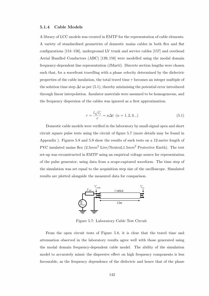
5.1.4 Cable Models

A library of LCC models was created in EMTP for the representation of cable elements.

A variety of standardised geometries of domestic mains cables in both flex and flat

configurations [154–156], underground LV trunk and service cables [157] and overhead

Aerial Bundled Conductors (ABC) [139, 158] were modelled using the modal domain

frequency-dependent line representation (JMartı). Discrete section lengths were chosen

such that, for a wavefront travelling with a phase velocity determined by the dielectric

properties of the cable insulation, the total travel time τ becomes an integer multiple of

the solution time step ∆t as per (5.1), thereby minimising the potential error introduced

through linear interpolation. Insulator materials were assumed to be homogeneous, and

the frequency dispersion of the cables was ignored as a first approximation.

τ =l√εrc

= n∆t (n = 1, 2, 3...) (5.1)

Domestic cable models were verified in the laboratory by small-signal open and short

circuit square pulse tests using the circuit of figure 5.7 (more details may be found in

Appendix ). Figures 5.8 and 5.9 show the results of such tests on a 12-metre length of

PVC insulated mains flex (2.5mm2 Live/Neutral,1.5mm2 Protective Earth). The test

set-up was reconstructed in EMTP using an empirical voltage source for representation

of the pulse generator, using data from a scope-captured waveform. The time step of

the simulation was set equal to the acquisition step size of the oscilloscope. Simulated

results are plotted alongside the measured data for comparison.

Figure 5.7: Laboratory Cable Test Circuit

From the open circuit tests of Figure 5.8, it is clear that the travel time and

attenuation observed in the laboratory results agree well with those generated using

the modal domain frequency-dependent cable model. The ability of the simulation

model to accurately mimic the dispersive effect on high frequency components is less

favourable, as the frequency dependence of the dielectric and hence that of the phase

142

Figure 5.8: Open Circuit Pulse Test - 2.5mm2 Mains Flex

velocity are ignored. The effects of dispersion manifest themselves in a time-spreading

of the measured reflected pulse on its return to the source, reducing the initially sharp

definition of its rising edge. The simulated pulse by contrast remains well-defined

following its transit. Though clearly a problem for studies in the MHz domain, for the

purpose of switching transients in the frequency range 10-500kHz, this discrepancy was

deemed acceptable.

Figure 5.9: Short Circuit Pulse Test - 2.5mm2 Mains Flex

The short circuit test of Figure 5.9 again gives a good reproduction of the time delay

for the propagation of a 75ns square pulse. The only major discrepancy is that due to

the necessary omission of proximity effects in the calculation of the series resistance,

the attenuation of the LCC model is less pronounced than that observed for the real

cable. This effect is compensated at the frequency of interest by the addition of a small

143

series resistance in the final simulation models.

5.1.5 Load Modelling

The local load for the laboratory rig simulations was modelled as a resistance, with

a small parallel stray capacitance determined from a frequency scan of the test load

bank.

5.1.6 Final Rig Model

The completed single-phase rig model is shown in Figure 5.10a. The interchangeable

source models are each depicted in increasing complexity by Figures 5.10b, 5.11a and

5.11b. For the purpose of the following comparative studies, a 50ms solution window

was specified to allow for a one-cycle settling time, and a solution time step of 20ns

chosen in line with the time-resolution of laboratory data.

(a) EMTP Simulated Laboratory Rig Model

(b) Capacitive Inrush Model

Figure 5.10: Laboratory Rig Model in ATPDraw and Capacitive Inrush Source

144

(a)

Equiv

ale

nt

AC

Model

(b)

PW

MM

odel

Fig

ure

5.11

:R

educe

dA

Can

dF

ull

PW

MS

ourc

eR

epre

senta

tion

s(A

TP

Dra

w)

145

5.1.7 Comparison of Generated Waveforms

Figures 5.12, 5.13 and 5.14 compare equivalent waveforms generated using the three

source variants with a sample capture taken from the laboratory data. The former is

a plot of current in the live terminal conductor (measured in the direction of positive

export), with the rising edge of the measured inrush lagging the positive-going voltage

zero by a quarter cycle (θi = 90o).

The capacitive model was found to give the best reproduction of the measured inrush

waveform, followed closely by the AC equivalent model. In both cases the magnitude

and slope of the current surge closely match the data, though the AC model is slightly

conservative in its estimate of peak current, falling short relative to capacitive inrush

model by approximately 1.5A. The introduction of the equivalent inrush capacitance

in both models allows for fine control of the angle of inrush θi, and as such the timing

of the rising edge can be tuned to match the data very closely.

The same cannot be said of the full PWM model, however, which despite giving a

reasonable reproduction of the overall wave-shape offers little in the way of controllability,

as evidenced by the inherent delay visible in the waveform of Figure 5.12. Such

behaviour is due primarily to a portion of the inrush current being determined by the

transformer saturation characteristic, which does not in itself account for the effects of

remnant flux in the core. Correct representation of such effects would likely provide

better control of the current front timing, but in order to do so, initial conditions

would need to be individually specified on a case by case basis. This requirement

would render the formulation of statistical studies, involving tens or hundreds of cases,

entirely impractical.

Measurable perturbations in the terminal voltage occur initially on closing the

electromechanical relays in the inverter disconnector. A second voltage peak may

also be observed in conjunction with the aforementioned current inrush. Figure 5.13

compares the simulated terminal voltage perturbation on CB closing with that obtained

by measurement. In this case, the perturbation is dominated by an oscillation between

the transformer output capacitor and line reactance. Since in each of the three source

models the components on the grid-side of the toroidal transformer are identical, there

146

Figure 5.12: Inrush Current Wavevorms for θi = 90o

is little to distinguish between their behaviours. Vmax anddV

dt maxin each case were

found to lie within 5% of the measured value, though some higher frequency components

in the measured results are absent from the simulations, most likely due to simplifying

assumptions in modelling of the filter circuit. The second pole closing operation is also

visible in the measured waveform, while coincident switching has been assumed in the

simulation models.

Reproduction of the secondary voltage perturbation was found to be somewhat

less straightforward. As can be seen from Figure 5.14, the measured dV consists of

a single voltage dip, with a magnitude around twice that of Figure 5.13, while the

rate of rise is reduced roughly fivefold. This behaviour is partially reproduced by the

Capacitive Inrush and AC models, but both also give rise to a lightly damped oscillation

following the initial peak, persisting for 1-2ms at a frequency of roughly 2kHz. This

discrepancy may be due either to an under-estimation of inherent damping in the supply

cables, or more likely the use of ideal components in the simulated notch filter network.

Additional refinement of the source models in the light of these differences shall be a

focus of future work. The PWM model significantly underestimates the peak voltage by

around 40%, and suffers also from the delay caused by a poorly initialised transformer

inrush characteristic.

147

Figure 5.13: Terminal Voltage Perturbation on Switch Closing

Figure 5.14: Terminal Voltage Perturbation on Inrush

5.1.8 Solution Efficiency

Table 5.2 summarises the scaling of overall solution time by source count and topology.

Solution times in CPU-seconds were logged for cases executed sequentially on a single

machine. Twenty executions were performed for each case and averaged solution times

148

normalised to that of the shortest case (5.2).

Tnorm. =Tsoln.Tmin

(5.2)

Table 5.2: Normalised Solution Time

Case Capacitive Inrush Model AC Equivalent Full PWM

1 Generator 1.0 1.83 2.072 Generators 1.53 2.07 2.324 Generators 2.13 2.72 3.76

For cases involving individual generators, significant CPU time savings can be made

by utilising a simple capacitive inrush source representation in place of the AC or

PWM equivalents. As the number of generators involved increases the relative economy

diminishes, though an absolute reduction in solution time is still clearly visible from

Figure 5.15.

Figure 5.15: Normalised Solution Time with Successive Doubling of Generator Count

5.1.9 Statistical Switch Definition

The laboratory rig model variants were adapted for use in system studies by replacing

the single-shot timed switches sw1, sw2, swt and swc with statistical equivalents.

Closing times for both poles of the disconnector were defined by a Gaussian distribution,

as corroborated by laboratory measurement. Closing times for the fictitious inrush

149

switch swi were modelled as a linear distribution over the measured range, in the

absence of more clearly defined behaviour.

In order to minimise the independent switch count in a given simulation, absolute

switch time distributions were converted to the following set of delay distributions:

1. Absolute closing time of first breaker pole: tsw 1

2. Breaker pole delay: ∆tsw 1−2 = tsw 2 − tsw 1

3. Inrush delay: ∆tsw 1−i = tsw i − tsw 1

4. Arbitrary cut-off delay: ∆tsw i−c = tsw c − tsw i

The newly defined delay quantities are depicted in Figure 5.16 with reference to a

typical output current waveform. Using this representation, the sequence of switching

operations within the generator model can be replicated by a cascaded master slave

representation as depicted in Figure 5.17.

Figure 5.16: Switch operating times as delay terms

150

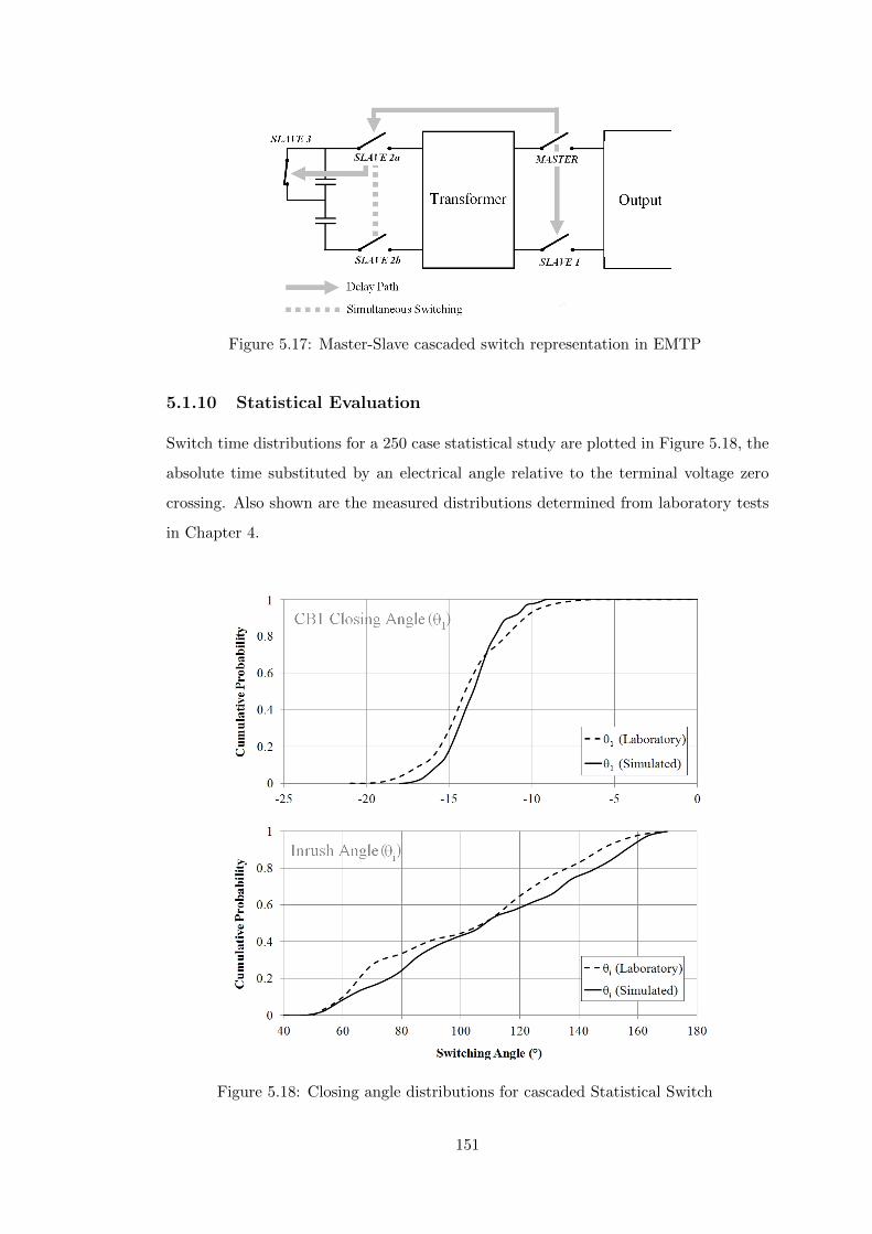
Figure 5.17: Master-Slave cascaded switch representation in EMTP

5.1.10 Statistical Evaluation

Switch time distributions for a 250 case statistical study are plotted in Figure 5.18, the

absolute time substituted by an electrical angle relative to the terminal voltage zero

crossing. Also shown are the measured distributions determined from laboratory tests

in Chapter 4.

Figure 5.18: Closing angle distributions for cascaded Statistical Switch

151

Having converted the time domain source model to a statistically determined one,

the single shot case of section 5.1.7 can be extended to many cases in order to verify

the dependence of peak currents and voltages on switching angle. Figure 5.19 compares

such a dependence of the measured inrush current peak on the angle θi, together with

that generated using statistically switched capacitive inrush model.

Of the three cases, the capacitive inrush model was found to give the best reproduction

of the θi − Imax relationship. The AC and PWM models each introduce a systematic

error associated with the fixed initial conditions governing residual transformer core

flux. A similar behaviour is noted regarding maximum voltage deviation. The dependence

of voltage transient magnitude on θi for the statistical capacitive inrush model is

compared with laboratory measurement in Figure 5.20. Two local loading scenarios

are presented, and good agreement of measurement and simulation observed in each.

Beyond θi ≈ 140o, ∆V2 reduces to a small value and the simulation results accordingly

become less well defined as the solver output summary is unable to distinguish between

the two peaks ∆V1 and ∆V2.

Figure 5.19: Dependence of peak current on inrush angle θi

The relationship between peak voltage and current by contrast is well represented

in the simulation case (Figure 5.21). Identical behaviour to that of the CI model was

observed with both EAC and PWM models, as the V-I characteristics are governed

those components common to each model. It can be safely assumed that the output

filter network and upstream cabling models are an adequate representation of their

hardware equivalents.

152

Figure 5.20: Dependence of peak voltage on switching angle θ

Figure 5.21: Peak Voltage vs Peak Current over 250 simulated switching events

5.1.11 Discussion of Test Set-up Model and Results

The merits and drawbacks of three alternative source representations have been discussed.

It has been shown that those SSEG switching operations of greatest interest may

be represented by means of the simplest simulation model - namely the equivalent

capacitive inrush model. This is an important finding as it is desirable to minimise

the computational burden posed by simulating large numbers of embedded generators,

where software limitations begin to impose practical constraints on the model’s extent.

For the purposes of small network studies and short simulation regimes, a model

explicitly representing the source (either as a PWM bridge or equivalent AC source) may

be employed. Though this additional complexity is unnecessary for the representation

of generator reconnection and inrush, it does afford a degree of flexibility in allowing

a single model topology to represent all permutations of switching operations. Subject

153

to the precise specification of initial conditions, these models are able to give excellent

results, but their increased complexity and associated solution inefficiency precludes

their applicability to extensive study.

5.2 Generic Domestic Model

5.2.1 Overview

Given the near infinite variety of domestic wiring and load configurations, the specification

of a typical domestic model is at best an exercise in the arbitrary. However, a number

of circuit features and wiring topologies common to domestic installations may be

identified (with reference to [156]), and some general assumptions may be made regarding

household load scenarios from the available aggregated demand figures [159]. This

section is concerned with formulation of a domestic cabling and load model in EMTP

for the purpose of SSEG switching studies.

5.2.2 Cable Models

A library of frequency-dependent cable sections was generated using the modal domain

travelling wave representation of Marti [160]. PVC insulated and shrouded cables in

both flat and round flex configurations were modelled with power conductor geometries

in the range of 1.5 − 6mm2.

One difficulty faced in modelling domestic wiring by this method is in specifying

the resistivity ρ of the ground medium. Given the variety of possible surface and

ballast materials (brick, concrete, wood, plasterboard, pvc conduit . . . ), and taking

into account the effects of moisture content and ambient temperature, values of ρ may

vary from 100 to tens of thousands of Ωm, and as such it is impossible to typify the

electrical properties of all surrounding media.

However, given the proximity of the protective earth to both power conductors,

it was assumed that the electrical characteristics of a cable should remain largely

independent of the properties of the ground medium. This is particularly true in

the case of building materials with a high volume resistivity, an assertion confirmed

by parametric study (see Appendix D). For the purpose of this study, a fairly large

ground resistivity value (500Ωm) was chosen, resulting in numerically stable models in

154

the majority of cases. An adjustment of ±5Ωm was necessary in certain instances in

which stability was found to be marginal.

5.2.3 Loads

A set of domestic load configurations was specified, as summarised in Table 5.3. First, a

Base load representing common background demand (refrigerator compressors, emergency

lighting, standby equipment etc.) was defined in line with the minimum average load

scenarios presented in [25]. Secondly, a Normal occupancy scenario supplements the

base case with a combination of linear and nonlinear loads to represent lighting, small

consumer appliances, computers and other low power equipment [92], based on typical

household demand [159].

Table 5.3: Domestic Load Scenarios

Load Configuration Magnitude Power Factor Stray Cap.

Base Load 160W 0.95 500pFNormal Load (Linear) +200W 0.95 500pFNormal Load (Nonlin.) +140W 0.5 470nFHeavy Load +800W 1.0 500pF

Finally, a Heavy load scenario is specified with reference to the generic UK LV

network model [22–25] by splitting the 11/0.4kV transformer capacity evenly among

all 384 supplied customers (approximately 1.3 kW). The difference between Normal

and Heavy load scenarios was assumed to be taken up by water/space heating and

cooking and, as such, is modelled purely as a resistance.

A small stray capacitance of the order of a few hundred pF was added in each

case, with the exception of the nonlinear load which incorporates an input capacitance

typical of a small power electronic interface (CFL, SMPS . . . ).

5.2.4 Source Model

Since generator reconnection is of most interest from an electromagnetic transient

standpoint, the capacitive inrush model (section 5.1.3) was chosen for all studies involving

the generic domestic circuit.

155

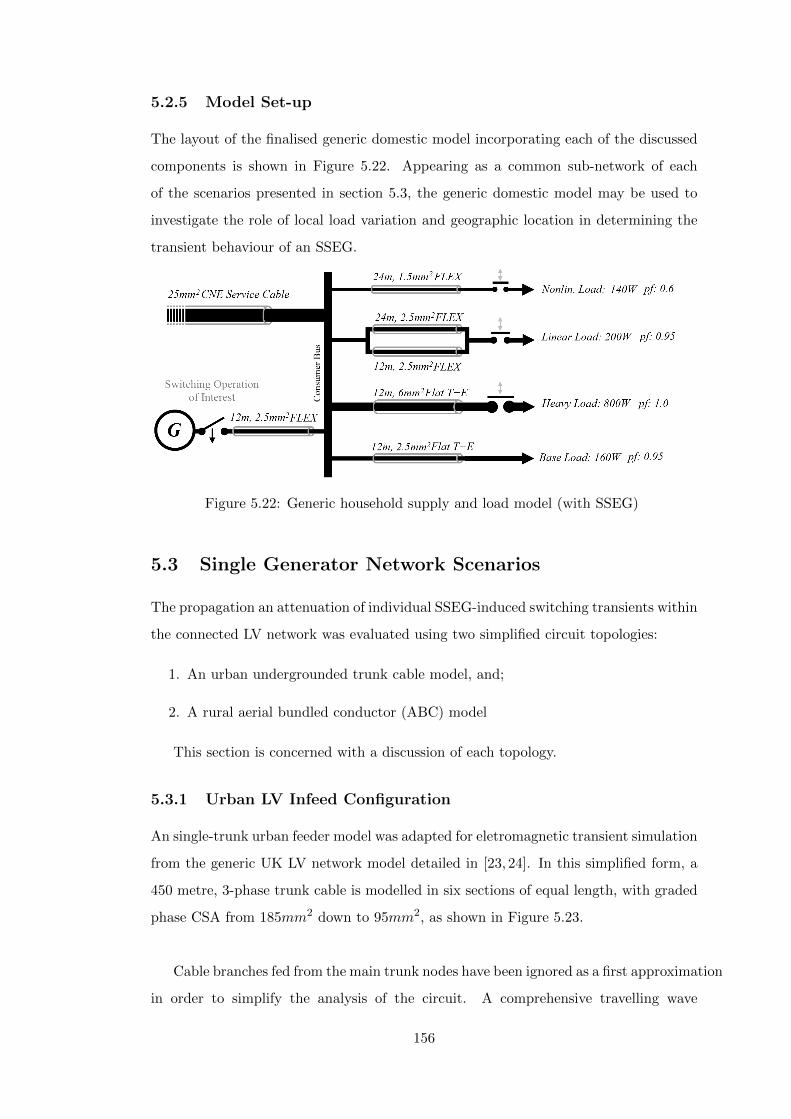
5.2.5 Model Set-up

The layout of the finalised generic domestic model incorporating each of the discussed

components is shown in Figure 5.22. Appearing as a common sub-network of each

of the scenarios presented in section 5.3, the generic domestic model may be used to

investigate the role of local load variation and geographic location in determining the

transient behaviour of an SSEG.

Figure 5.22: Generic household supply and load model (with SSEG)

5.3 Single Generator Network Scenarios

The propagation an attenuation of individual SSEG-induced switching transients within

the connected LV network was evaluated using two simplified circuit topologies:

1. An urban undergrounded trunk cable model, and;

2. A rural aerial bundled conductor (ABC) model

This section is concerned with a discussion of each topology.

5.3.1 Urban LV Infeed Configuration

An single-trunk urban feeder model was adapted for eletromagnetic transient simulation

from the generic UK LV network model detailed in [23, 24]. In this simplified form, a

450 metre, 3-phase trunk cable is modelled in six sections of equal length, with graded

phase CSA from 185mm2 down to 95mm2, as shown in Figure 5.23.

Cable branches fed from the main trunk nodes have been ignored as a first approximation

in order to simplify the analysis of the circuit. A comprehensive travelling wave

156

Figure 5.23: SSEG feeding an urban underground LV circuit

analogue of the UK generic LV network is presented in Chapter 6. The sectored

geometry of the trunk cable [111, 157] is approximated by an equivalent circular cable

pipe model as discussed in Chapter 2.

A 50-metre length of single-phase 25mm2 service cable links the consumer bus of the

generic domestic model to phase A of any of the six trunk nodes (x = 75m → 450m).

In this way, the combined effect of a generator’s local load and its position relative to

the LV terminals of the 11/0.4kV transformer may be investigated.

Each of the aforementioned trunk nodes, together with the transformer terminal

(x = 0m) and consumer bus, is fitted with a TACS filtered voltage probe. This allows

straightforward identification of high frequency voltage transient peaks in which the

magnitude lies below the steady-state amplitude of the grid supply voltage (< 325V ).

The 11kV grid supply and circuit (not shown) are represented as an ideal voltage

source behind a parallel source/surge impedance network [120], and a 1500-metre length

of 11kV cable, modelled in the same fashion as the LV trunk cables.

5.3.2 Rural LV Infeed Configuration

A similar topology was specified for investigating an SSEG connecting into a rural

overhead LV circuit. In the absence of an established generic LV model for the simulation

of rural networks, a library of wood-pole mounted Aerial Bundled Conductors (ABC)

as standardised in [139] was created in line with typical DNO guidelines for new and

replacement lines [158]. A trunk circuit of length 1400m was constructed using line

157

Figure 5.24: SSEG feeding a rural overhead LV circuit

spans of 50m, with graded CSA from 120mm2 down to 70mm2 as shown in Figure 5.24.

The consumer is fed from one of the trunk nodes by 100m of single phase 35mm2

service line, for a total effective circuit length of 500-1500m. A 3.6km section of the

11kV bare conductor OHL circuit upstream of the transformer (not shown) is modelled

according to [161].

5.3.3 Ground Resistivity

In both the urban and rural models, ground resistivity for the LV distribution circuit

was assumed to be 100Ωm as per the guidelines of [120]. This is in contrast to the

higher resistivity ground (500Ωm) chosen for the domestic cable models. The effects of

adjacent conductive media (pipelines, telegraph cables etc.) have been ignored for the

generalised case.

5.4 Switching Transient Simulation Results

There follows a summary of simulation results for scenarios with a single generator

feeding each of the simplified LV circuits. Unless otherwise specified, statistical data is

based on a regime of 100 test cases in each scenario, with generator switch distributions

according to section 5.1.9.

5.4.1 Urban LV Feeder Simulation Results

Transient voltage magnitudes were recorded at each node (x = 0, 75, ... 450m) for each

of the generator feed-in locations xg. Figure 5.25 shows the mean voltage magnitude

158

Figure 5.25: Range of urban feeder voltage magnitude profiles for xg = 75m andxg = 450m (minimum load)

profiles under minimum load conditions, for generators connected adjacent to the

11/0.4kV transformer (xg = 75m) and at the remote end of the feeder (xg = 450m).

The range of values obtained in both cases is illustrated by means of the 5th and 95th

percentile values, also plotted in Figure 5.25.

It is clear that the voltage magnitudes encountered with a single generator feeding

an urban cable network are near immeasurable ( 0.01 pu in the worst case). However,

it is of interest to note the effect of position on the voltage profile. The results indicate

a linearly attenuated transient voltage magnitude in the region x = 0 → xg, and a

subsequent plateauing effect along the circuit downstream of xg. This is more clearly

illustrated by Figure 5.26a. Here, the mean spike magnitude profile is plotted explicitly

for each of the six in-feed positions.

The same plot is reproduced in Figure 5.26b, with a larger voltage scale to include

the range of simulated voltages at the consumer bus (vcon) for each value of xg. It is

clear that the magnitude of the voltage transient is greatly curtailed by the short length

of service cable linking the consumer bus and the LV trunk node. In this instance, the

results is a mean attenuation of 5.5V from an initial magnitude in the range 7.0-9.5V.

Despite this observation, the magnitudes encountered remain of no concern from the

standpoint of either insulation coordination or electromagnetic compatibility.

159

(a) Mean urban voltage magnitude profiles by in-feed location (min. load)

(b) Mean urban magnitude profiles including consumer bus (min. load)

Figure 5.26: Voltage Magnitude Profiles on a One-Line Urban Feeder

160

Figure 5.27: Magnitude profiles for xg = 75m and 450m under minimum and heavyload conditions (urban)

The final plot of figure 5.27 illustrates the effect of consumer bus loading on transient

peak voltage. Mean magnitude profiles are illustrated for generators at xg = 75m, 225m

and 450m for the minimum load scenario. This is overlaid with the same set of profiles

generated under the heavy load scenario.

It is clear that some curtailment of the transient voltage is attributable to the local

load condition, the extent of this effect being dependant on the customer’s position

relative to the transformer LV bus. Switching under heavy load conditions for example

will typically reduce peak voltages by around 10% for a remotely connected customer,

compared to the minimum load case. For an equivalent customer connected close to

the transformer, the effect is negligible.

161

5.4.2 Rural LV Feeder Simulation Results

The analyses of the previous section were repeated for the rural feeder model, this

time with customers connected in 200m intervals up to 1400m from the transformer.

Figure 5.28 illustrates the effect of feed-in position on the expected transient voltage

magnitude.

Figure 5.28: Range of rural feeder voltage magnitude profiles for xg = 400m andxg = 1400m (minimum load)

The behaviour of the rural circuit is very similar to the urban case in this regard,

though some elevation in voltage is to be observed in the rural circuit. The gradient

of the transient magnitude profile is approximately doubled over an equivalent length

of overhead circuit, with mean voltages rising to around 17V for a generator located

1500m from the LV terminals of the pole transformer.

The dependence of dV on xg is once again a linear one as can be seen from Figure

5.29, but unlike the underground circuit of the urban case, the attenuation attributable

to the single phase overhead service line is comparatively minimal, despite its increased

length. A reduction in magnitude of only 1-2V can be expected to occur in propagation

from the customer bus to its adjacent trunk node.

Finally, the attenuation of a typical transient due to local load conditions is somewhat

less pronounced in the rural case. An equivalent reduction of 10% in the transient

162

Figure 5.29: Mean rural voltage magnitude profiles by in-feed location (min. load)

voltage magnitude under heavy load for example requires approximately 800m of ABC

between the consumer and the LV transformer (in contrast to 450m of underground

cable in the urban case). This is illustrated in Figure 5.30.

Figure 5.30: Magnitude profiles for xg = 400m and 1400m under minimum and heavyload conditions (rural)

163


In this chapter, simulation models for the representation of embedded generators rated

below 16A/phase have been developed and compared according to their flexibility and

solution efficiency. A generic model for the representation of domestic power circuitry

has been proposed and, in conjunction with simplified single trunk models of urban

and rural LV utility circuits, used to estimate transient voltage magnitudes due to

generators switching at different radial feeder positions. Principal conclusions are as

follows:

• The most severe generator switching transients (those associated with grid-reconnection)

may be modelled using a simplified capacitive inrush circuit representation, ignoring

all components behind the inverter DC bus.

• Relay pole closing and inrush inception may be accurately reproduced by means

of a cascaded master-slave switch representation, useful for statistical/systematic

study in EMTP.

• Typical simulated transient voltage magnitudes are extremely low for simulations

involving single generators, with worst cases of 1.03 and 1.06 p.u. for simplified

urban and rural network topologies respectively.

• Simulated voltages were found to be largely independent of localised loading

conditions.

Chapter 6 builds on this work, using the developed source models to investigate

the cumulative effect of multiple generators switching in response to common network

conditions.

164

Chapter 6

Cumulative ElectromagneticTransient Impact of SSEG

Building on the laboratory and simulation results of Chapters 4 5, a suite

of cumulative impact studies was drawn up to assess the combined impact

of multiple generators switching in response to common stimuli. In order

that these simulation studies could be performed, it was necessary to develop a best

optimised EMTP-ATP LV network model, as distinct from the simple one-line source

evaluation model presented in Chapter 5. This work has resulted in the development

of a complete travelling-wave equivalent of a 400/230V circuit, as broadly defined in

the generic UK LV distribution network.

The explicit representation of such extensive networks and large numbers of generators

presents its own challenges in terms of complexity and computational efficiency, and

there is a need to be mindful of the practical operating limits of the software. Clearly,

the network topology itself shall have some effect on the results of a given simulation,

but given the variety of LV network configurations that might be encountered, consideration

of all possible scenarios would be extremely time-consuming. An approach based on

DNO-approved generic models has therefore been adopted as a first approximation,

allowing these results to tie in with other studies based on generic networks [22–25].

Future work may then begin to consider the nuances of various network configurations.

In this chapter, an analysis of the various design choices and constraints and the

resulting hierarchical network models is undertaken. A set of simulation scenarios is

proposed based on generator penetration, using the capacitive source representation

165

developed in Chapter 5 (Figure 5.10b), and a variety of network loading profiles. The

results of extensive statistical simulations are presented and discussed in the sections

that follow.

6.1 Generic Low-Voltage Network Models

6.1.1 The Generic UK LV Network

The DNO-approved generic UK LV network as presented in [25] is depicted in figure 6.1.

The model consists of a parallel pair of 33/11kV transformers supplying six identical

11kV feeders. Each 11kV feeder supplies eight 400V buses through 500kVA 11/0.4kV

transformers, and each bus in turn supplies four feeders supplying 384 evenly distributed

customers. The total circuit length from 11kV bus to most remote customer node is

1.5km. Table 6.1 gives a breakdown of the total number of downstream consumer nodes

at each level of the model.

Figure 6.1: Generic UK LV Network Model

166

Table 6.1: Total Downstream Customer Nodes by Location

Position Customers Minimum Load (kVA) Maximum Load (kVA)

11kV Bus 18432 3000 2400011kV Feeder 3072 500 4000400V Bus 384 61.4 500400V Feeder 96 15.4 125

Load is assumed uniformly distributed across the network, ranging from a minimum

of approximately 160VA per customer up to a maximum defined by the rating of the

500kVA transformers (approximately 1300VA per customer).

For the purpose of electromagnetic transient simulation, modelling of the complete

11kV and 400V radial network with its 18,432 individual consumer nodes was deemed

impracticable within the constraints imposed by even the most liberally specified EMTP

listsize variables. It was noted, however, that for transient overvoltages generated on

the 400/230V side of the transformer, the effect of coupling to the 11kV circuit should

be negligible. Indeed, an overvoltage of almost 30 p.u. would be needed to register any

significant disturbance which, though theoretically plausible in the case of lightning

induced overvoltages from strikes to nearby structures, is at least an order of magnitude

higher than that expected to occur due to switching.

The interaction between neighbouring 400V buses was, therefore, ignored for the

purposes of this study, and only one 400/230V circuit modelled explicitly. The 11kV

circuit upstream of the 500kVA transformer is represented simply by means of a 1.5km

length of 3-phase underground cable, as in the simplified models of Chapter 5. A

one-line diagram of the LV bus/feeder sections to be modelled is shown in Figure 6.2.

6.1.2 Modelling Constraints

The permissible extent of a simulation model in EMTP-ATP is constrained by a set

of variable dimensioning limits defined in the listsize file of the EMTP installation.

Those limiting values of particular interest are summarised in Table 6.2. Default values

for the standard atpmingw software build packaged with the ATP easy installer [162]

are listed. Equivalent limiting values are also given for an alternative software build

(gigmingw) available from [163] which, though potentially less stable than the standard

release, is capable of handling simulation models with far greater volumes of network

167

Figure 6.2: 400/230V LV Network Layout

168

elements [164].

Table 6.2: Limiting Listsize Variables for Large Network Models [95]

Variable Description atpmingw gigmingw

LBUS Maximum number of network nodes 6,000 100,000

LBRNCH Maximum number of network branches 10,000 200,000

LSWTCH Maximum number of switches, 1,200 6,000diodes and thyristors

Storage space for frequency-dependentLFSEM lines/cables ≈ 7×Number of poles 100,000 400,000

required to represent branch Z0 and A1

Storage space for frequency-dependent

LFD line/cable transformation matrices ≈ 2N2 3,000 12,000for each unique N-phase line

LHIST Additional frequency-dependant storage 15,000 60,000≈ 15×Number of coupled phases

In predicting potential limit violations in either ATP distribution, the following

quantities are defined with reference to the generic LV model, as illustrated in more

detail in Figure 6.3.

• nL: Number of customer load buses per feeder = 96

• ng: Number of generator buses per feeder ≤ 96

• nc3φ: Number of 3-phase cable segments per feeder = 20

• nc1φ: Number of 1-phase cable segments per feeder = 96

• nf : Total Number of 400/230V feeders

• nm: Total Number of measurement positions

6.1.2.1 Node Limits

The number of nodes required to represent a given network scenario may be estimated

by Equation (6.1), where NL is the number of nodes required to represent an aggregated

customer load (3 ), Ng the node count of the chosen generator model (25 → 43 ) , Nm the

169

(a) 400/230V Bus

(b) Individual Feeder Detail

Figure 6.3: Generic LV Network Modelled in EMTP

170

node count per phase for each voltage measurement group (≈15 ) and kN is a constant

accounting for network nodes necessary for representing the network upstream from,

and including, the LV transformer (≈30).

nnode ≈ nf × (nLNL + ngNg + 4nc3φ + 2nc1φ) + 3nmNm + kN (6.1)

Table 6.3 summarises the predicted node counts by generator model and SSEG

% penetration (ρg) on a four-feeder generic LV network. It is clear that based on

node/bus counts alone, only low penetration scenarios can be fully represented using

the standard atpmingw distribution. For a ρg scenarios in excess of 25%, the additional

capacity afforded by the gigmingw distribution becomes necessary, even when using the

minimal-node capacitive inrush generator model.

Table 6.3: Approximate Node Count for Increasing SSEG Penetration Scenarios

Generator Modelρg

25% 50% 100%

Capacitive Inrush 4,900 7,300 12,100AC Equivalent 6,500 10,600 18,600Full Inverter 6,600 10,800 19,000

6.1.2.2 Branch Limits

Branch counts for the same circuit may be estimated by Equation (6.2) where BL

is the branch count of an aggregate customer load (4), Bg the branch count for the

chosen generator model (44→ 128) and Bm is the number of branches in a single phase

measurement block (15). The constant kB is used to factor in those network branches

upstream of the 400V bus (≈50). Predicted branch counts are summarised in Table

6.4.

nbranch ≈ nf × (nLBL + ngBg + 4nc 3φ + 2nc 1φ) + 3nmBm + kB (6.2)

171

Table 6.4: Approximate Branch Count for Increasing SSEG Penetration Scenarios

Generator Modelρg

25% 50% 100%

Capacitive Inrush 7,300 11,700 20,600AC Equivalent 10,000 17,100 31,300Full Inverter 15,400 27,800 52,800

Once again, predicted component counts greatly exceed the limits imposed by the

standard installation in all but the lowest penetration scenarios. The large branch

counts required for high ρg scenarios can, therefore, only be expected to compile with

the gigmingw distribution.

6.1.2.3 Switch Limits

Possibly the most restrictive of the listsize variables, LSWTCH limits the total number

of individual switches (timed, statistic and systematic), diodes, thyristors and valves

for an individual simulation case. Since the switch count is dependent on the choice of

generator model as well as the total number of embedded generators, an estimate of

the switch count can be obtained from Equation (6.3), where Sg is the switch count for

the chosen generator model (6 for the capacitive inrush and AC equivalents, 15 for the

PWM bridge). Table 6.5 gives the expected switch count for each of the penetration

scenarios already discussed.

nswitch = nfngSg (6.3)

Table 6.5: Approximate Switch Count for Increasing SSEG Penetration Scenarios

Generator Modelρg

25% 50% 100%

Capacitive Inrush 576 1,152 2,304AC Equivalent 576 1,152 2,304Full Inverter 1,440 2,880 5,760

Not only is the switch limit (1200 ) exceeded for ρg in excess of 50%, the switch count

for maximum SSEG penetration using the full inverter model is very close to the limit

for the giga version (6000 ). It is advised where possible to use either the Capacitive

Inrush or Equivalent AC models so as to avoid unwanted errors should LSWTCH be

172

exceeded, and to minimise the total number of partial Y-matrix re-traingularisation

operations associated with the opening and closing of switches.

6.1.2.4 Frequency-Dependent Line Limits

The remaining three listsize variables governing use of frequency-dependent transmission

lines are independent of ρg, as the topology of the cable network does not change

between simulations. The required values for LFSEM, LFD and LHIST can be estimated

by the equations in Table 6.6.

Table 6.6: Approximate Listsize Values for Frequency Dependent Line Modelling

Variable Approximation Single Feeder 4 Feeders

LFSEM 14nfPZ0 (4nc3φ + 2nc1φ) 76,000 305,000

LFD 2 (4uc3φ + 2uc1φ)2 800 800

LHIST 15nf (7nc3φ + 2nc1φ) 5,200 21,000

PZ0 and PA1 are the number of poles required to fit Z0 and A1 respectively for each

branch. A curve fitting of 20 points per decade from 1mHz up to 10MHz was found

to give good results for all cable geometries, from 25mm2 single phase service lines

up to the 185mm2 three-phase trunk cable, with the number of poles rarely exceeding

PZ0 = PA1 ≈ 20. The quantities uc1φ and uc3φ are the number of uniquely defined single

and three-phase cables respectively. Since it is desirable to minimise these quantities

as far as possible, only a limited range of conductor grades have been included in

the finalised generic LV model, consistent with the specification of the generic UK LV

model.

6.1.2.5 ATPDraw Display Limits

In order that the finalised generic model be portable for further application, the display

limitations of typical graphical preprocessors should also be adhered to. ATPDraw, the

most commonly used preprocessor to EMTP-ATP imposes its own constraints on the

number of objects in a single circuit. In addition, since the finished model shall include

hundreds of generators, loads and cables, it is desirable to make maximal use of the

circuit compression function in order to avoid a sprawling and convoluted network

173

topology. The number of hierarchical compressed groups that may exist in a single

model is also constrained. Limiting values are summarised in Table 6.7.

Table 6.7: ATPDraw Display Limits

Constraint Value

Object Limit 10,000Group Limit (pre version 5.6) 255Group Limit (version 5.6 onwards) 2047

Estimates of the object and group counts may be obtained from Equations (6.4)

and (6.5). The number of circuit objects is approximately equal to the number of

circuit branches plus the number of compressed groups. The compressed group count,

in turn, assumes a hierarchical structure in which each aggregated customer load and

each generator is assigned its own group. Customers are then compressed into groups

of six to be fed from each of sixteen LV trunk nodes, all of which are further compressed

into a single LV feeder group. This hierarchical structure is depicted in Figure 6.4.

nobjects ≈ nbranch + ngroups (6.4)

ngroups ≈ nf ·(

7

6nL + ng + 1

)+ nm (6.5)

The ATPDraw object and group counts are summarised in Table 6.8 for different

penetration scenarios on a four-feeder network. Use of the capacitive inrush generator

model is assumed.

Table 6.8: Approximate Object/Group Counts for Different SSEG Penetrations

Countρg

25% 50% 100%

Objects 7,800 12,400 20,500Groups 560 650 850

It is clear from a comparison of Tables 6.7 and 6.8 that in order for the generic LV

model to be useful, there is necessarily a major constraint on extent and complexity

imposed by the display limits of the GUI. Maximal use of the gigamingw distribution’s

expanded capabilities is, therefore, unachievable on practical grounds. It can be seen

that for even low penetration scenarios, the anticipated object count is close to the

174

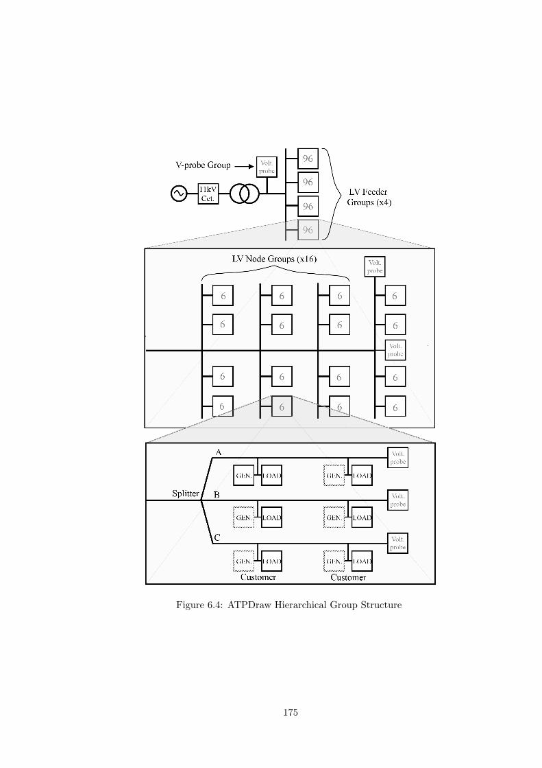
Figure 6.4: ATPDraw Hierarchical Group Structure

175

allowable limit of 10,000, and indeed some further aggregation of consumer loads has

been necessary in order to obtain a functional 50% ρg model.

6.1.3 Consideration of Solution Efficiency

The inherent complexity of models for the purpose of cumulative generator impact

studies means that significant computational power is required in order to generate a

statistically significant number of results. It is desirable, therefore, that the time step

be as large as possible without compromising the solution accuracy, and also that the

extent of the solution time window be minimised.

Node and branch economy is achieved by modelling the consumer as a single lumped

equivalent RL load connected directly to the single-phase service line of the LV network.

The short 12m lengths of cable that appear in the generic domestic model of Chapter

5 are omitted here, being replaced by small equivalent series resistances. The shortest

travel time of the model becomes that of the 25m service line, and the maximum

permissible time-step is doubled accordingly.

This economy is partially negated by the need to accommodate switching operations

on all three phases. As such, the solution time window has to be extended relative to

the single phase case by2

3of a cycle in order to guarantee that transient waveforms

in phases B and C are correctly recorded. The resulting solver setup requires a time

step ∆t of 40ns for simulation over a window Tmax=60ms for a total of 1.5 million data

points per voltage or current probe.

6.1.4 Switch Control

While the specification of master-slave switching arrangements is straightforward for

single generator studies, switch control becomes considerably more complex in scenarios

involving multiple sources. Ideally, each generator in the system would have its own

independent master-slave arrangement, but the number of independent switches allowed

in any one study is limited by statistical practicality to five [165]. Since as many as 192

generators split across three phases are to be simulated at the same time, an elaborate

arrangement of slave switch control paths must be employed.

176

Selecting one generator in phase A of the first feeder as a master, each other

generator becomes a slave unit with a delay term determined by the phase arrangement

of that generator (A=0ms, B=6.667ms, C=13.333ms). In this way, the switch time

distribution of the first closing pole of each disconnector is maintained, but a small offset

is introduced in each case, dependent on the actual closing time of the master switch.

Since the standard deviation of this offset is very small, being equal to the standard

deviation of the master switch pole, this arrangement may be deemed an acceptable

approximation to coincident independent switching behaviour. The arrangement of

switch delay paths is depicted in Figure 6.5

6.1.5 Simulated Urban Single Feeder

The completed single LV feeder model is depicted in Figures 6.6 and 6.7. By limiting

the model extent to only one feeder, 96 customers may be represented explicitly, each

with its own incoming service cable.

6.1.6 Urban LV Network - Four Feeders

As discussed, the object limits of ATPDraw become prohibitive for very large models

and as a result a complete 4-feeder model cannot simply be generated using carbon

copies of Figure 6.6. The LV node groups in this case are simplified by lumping each

customer phase-pair into a single equivalent load at the terminal of a 50m service cable

as depicted in Figure 6.8. In this way, all four feeders may be represented as shown in

Figure 6.9.

6.1.7 Generic Rural Network

In order to assess the cumulative impact of generators in rural networks, it was necessary

to also develop a representative rural LV circuit. In the absence of an established

reference network model, a topology based on that of the generic UK LV network

was adopted, but with a geographic load density around one tenth that of the urban

network, as in [92]. The network itself is a single feeder arrangement constructed using

aerial bundled conductor (ABC) cable models in 35, 70 and 120mm2 CSA, suspended in

50m spans from 9m tall wood poles as recommended by DNO planning guidelines [158].

The rural LV feeder structure is depicted in Figure 6.10, while Figure 6.11 is the

177

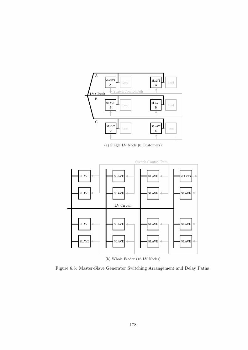
(a) Single LV Node (6 Customers)

(b) Whole Feeder (16 LV Nodes)

Figure 6.5: Master-Slave Generator Switching Arrangement and Delay Paths

178

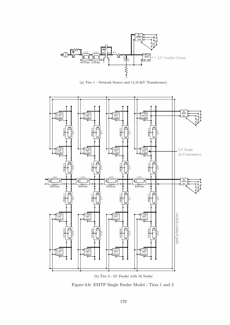
(a) Tier 1 - Network Source and 11/0.4kV Transformer)

(b) Tier 2 - LV Feeder with 16 Nodes

Figure 6.6: EMTP Single Feeder Model - Tiers 1 and 2

179

Figure 6.7: EMTP Single Feeder Model - Tier 3 - 6 Customer Nodes

Figure 6.8: EMTP Four Feeder Model - Reduced Tier 3 Group

180

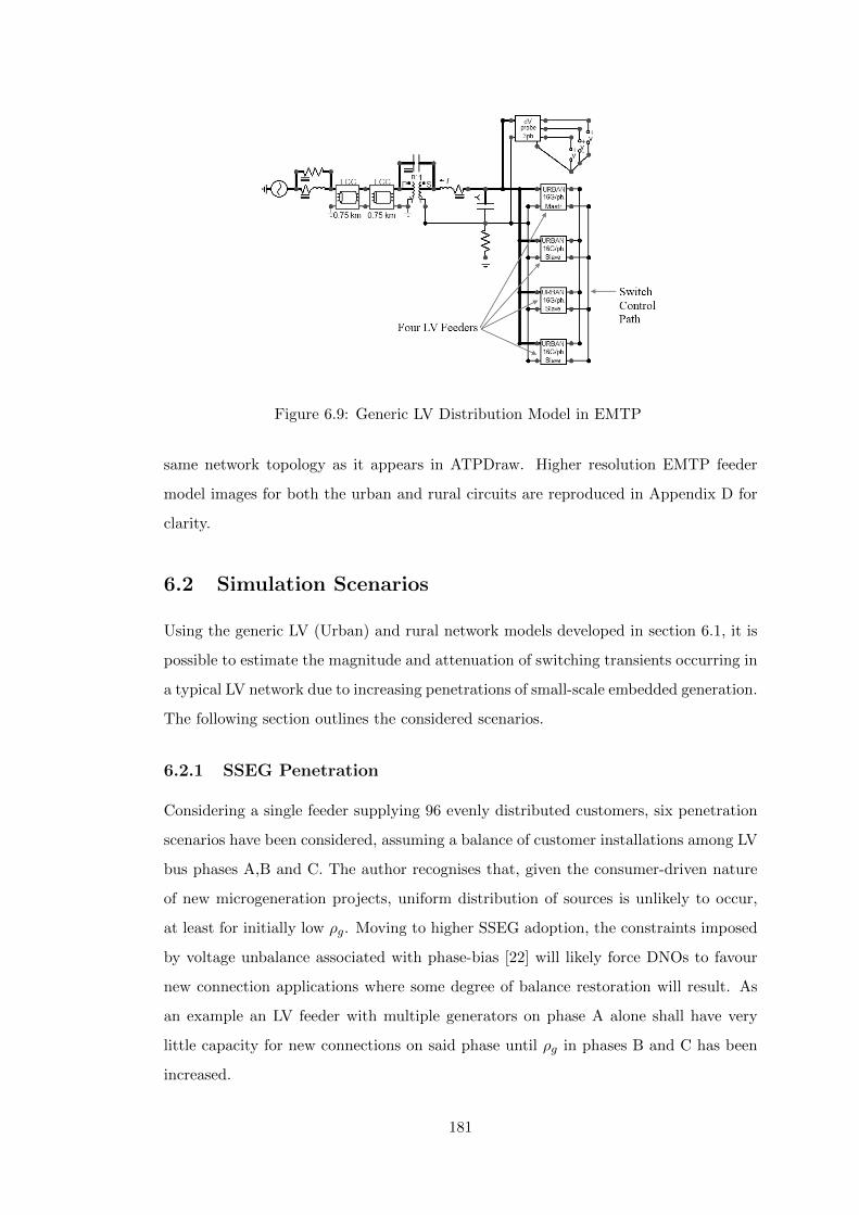
Figure 6.9: Generic LV Distribution Model in EMTP

same network topology as it appears in ATPDraw. Higher resolution EMTP feeder

model images for both the urban and rural circuits are reproduced in Appendix D for

clarity.

6.2 Simulation Scenarios

Using the generic LV (Urban) and rural network models developed in section 6.1, it is

possible to estimate the magnitude and attenuation of switching transients occurring in

a typical LV network due to increasing penetrations of small-scale embedded generation.

The following section outlines the considered scenarios.

6.2.1 SSEG Penetration

Considering a single feeder supplying 96 evenly distributed customers, six penetration

scenarios have been considered, assuming a balance of customer installations among LV

bus phases A,B and C. The author recognises that, given the consumer-driven nature

of new microgeneration projects, uniform distribution of sources is unlikely to occur,

at least for initially low ρg. Moving to higher SSEG adoption, the constraints imposed

by voltage unbalance associated with phase-bias [22] will likely force DNOs to favour

new connection applications where some degree of balance restoration will result. As

an example an LV feeder with multiple generators on phase A alone shall have very

little capacity for new connections on said phase until ρg in phases B and C has been

increased.

181

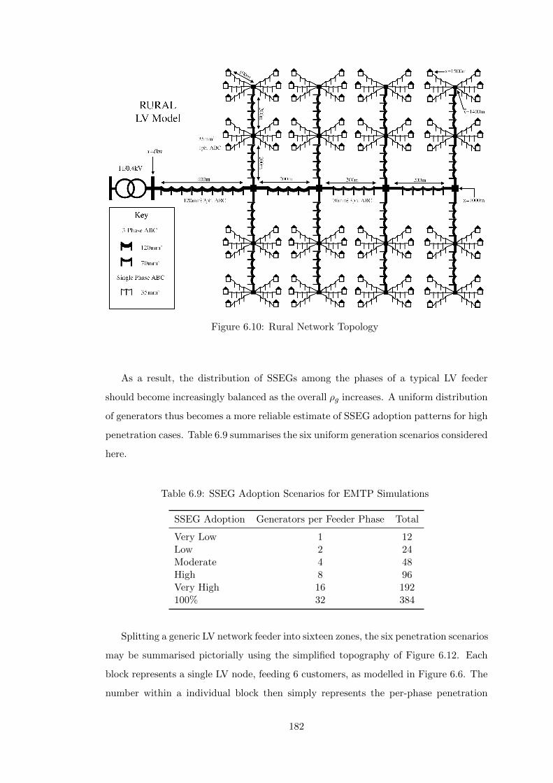
Figure 6.10: Rural Network Topology

As a result, the distribution of SSEGs among the phases of a typical LV feeder

should become increasingly balanced as the overall ρg increases. A uniform distribution

of generators thus becomes a more reliable estimate of SSEG adoption patterns for high

penetration cases. Table 6.9 summarises the six uniform generation scenarios considered

here.

Table 6.9: SSEG Adoption Scenarios for EMTP Simulations

SSEG Adoption Generators per Feeder Phase Total

Very Low 1 12Low 2 24Moderate 4 48High 8 96Very High 16 192100% 32 384

Splitting a generic LV network feeder into sixteen zones, the six penetration scenarios

may be summarised pictorially using the simplified topography of Figure 6.12. Each

block represents a single LV node, feeding 6 customers, as modelled in Figure 6.6. The

number within a individual block then simply represents the per-phase penetration

182

(a) Tier 1 - Network Source and 11/0.4kV Transformer)

(b) Tier 2 - LV Feeder with 32 Nodes (Three Customers per Node)

Figure 6.11: EMTP Rural Feeder Model

183

for for that LV node (max. 2 generators/phase for a total of 6). A similar pictorial

representation may be seen in Figure 6.13 for the thirty-two customer groups of the

rural equivalent network (Figure 6.11). A different notation is used here as only one

customer is supplied per single-phase service line in the rural case, halving the size of

a customer grouping to 3. An empty block in both cases indicates that no SSEG feeds

that LV node (load only).

(a) Very Low (3%) (b) Low (6%) (c) Moderate (12.5%)

(d) High (25%) (e) Very High (50%) (f) 100%

Figure 6.12: Urban Feeder Penetration - 16 LV Blocks of 6 Customers Each (2Customers per Phase, dot indicates presence of 1 SSEG per phase at a node)

6.2.2 Customer Load

Customer load is assumed to be uniformly distributed throughout the network, with

each customer modelled as a series linear RL branch based on average domestic load

power factor, with shunt stray capacitance of a few tens of picofarads. No diversity

in the load is taken into account here. Maximum and minimum load conditions are

defined as in Chapter 5 to be 160VA and 1300VA respectively, and a third typical load

of 500VA is arbitrarily defined. A no-load condition is also considered in order to define

the lower limits of statistical current distributions for each ρg case. Load configurations

are summarised in Table 6.10.

184

(a) Very Low (3%) (b) Low (6%) (c) Moderate (12.5%)

(d) High(25%) (e) Very High (50%) (f) 100%

Figure 6.13: Rural Feeder Penetration - 32 LV Blocks of 3 Custmers Each (1 Customerper Phase, dot indicates presence of 1 SSEG per phase at a node)

Table 6.10: Consumer RL Load Configurations for Network Models

Condition Load VA Cos(θ) Feeder kVA

Minimum 160 0.95 15Typical 500 0.95 48Maximum 1300 0.95 125No Load 1 1 0.1

6.2.3 Voltage and Current Probes

Four sets of voltage probes are connected at various points throughout the LV network

models in order to detect the magnitude of voltage perturbations due to generator

switching events. Each voltage probe is connected into the circuit via a notch filter

based on that used in [80], to remove any fundamental power frequency component

from the results. The positions of the measurement blocks relative to the 500kVA

transformer LV bus (x = 0) are summarised in Table 6.11. In both cases, Block 1 is

located at the transformer LV terminals, while Block 4 is a set of single phase probes

connected to the most remote consumer bus in each phase (see Figures 6.6, 6.7 and 6.11)

185

Table 6.11: Voltage Measurement Block Positions

ModelVolt Probe Position

Block 1 Block 2 Block 3 Block 4

Urban x = 0m x = 300m x = 450m x = 500mRural x = 0m x = 1, 000m x = 1, 400m x = 1, 500m

Current probes are located on the LV winding of the 11/0.4kV transformer to

measure the peak cumulative inrush current drawn from the grid due to coincident

switching operations.

6.2.4 Solution Time

For any statistical simulation study, the processing requirements are heavily dependent

on the number of non-concurrent switching operations, and as a consequence the total

solution time shall depend on the penetration scenario being considered. Using a time

step of 40ns over a window of 60ms, solution times of 250-case statistical studies were

found to increase with ρg from 10 to 72 hours on a typical laboratory workstation

(2.8GHz dual core, 3GB RAM).

6.3 Simulation Results

The following section summarises the results obtained from simulations of each of

the outlined generator/load scenarios. Statistical data is generated from data sets,

each consisting of 250 repeat cases with switch closing and delay times statistically

distributed in the same manner as in Chapter 5. Results are presented by network

topology, starting with the urban single feeder model and progressing to the generic

four-feeder and rural models.

6.3.1 Urban Single-Feeder Model

6.3.1.1 Current Transients (Urban Feeder)

The plot in Figure 6.14a shows the statistical distribution of peak currents measured

at the LV terminal of the 500kVA transformer. A normalised combined data set of all

three phases (750 results per curve) is plotted. Only the no load and maximum load

conditions are shown here to avoid overlapping ranges, and the lowest ρg scenarios are

omitted for clarity. The dashed vertical line at approximately 245A marks the phase

186

(a) Statistical Distributions of LV Bus Peak Current by SSEG Penetration (All Phases)

(b) Dependence of Inrush Current Statistics on Generator Count.

Figure 6.14: Cumulative Network Inrush Currents - Urban Feeder

current amplitude under maximum load condition with no SSEG (assuming the supply

voltage to be approximately 240Vrms), and forms the a base line for that condition,

much as I = 0A forms the base line for the no load case.

It can be seen that for a given load scenario, an increase in the number of concurrent

SSEG switching operations leads to an increase in the mean current magnitude above

the base line. This is a linear relationship as can be seen from Figure 6.14b. By contrast,

the dispersion of peak current distribution displays a square-root proportionality with

ρg.

187

Ipk ∝ ρg σIpk ∝√ρg

It is also noted that the deviation, skew and kurtosis of current distributions are

all independent of the pre-existing load condition. Thus current distributions in the

full load case are the same as at no load, but offset by a value equal to the phase load

current amplitude (245A in this case). Given that the magnitude of the inrush for each

generator is governed by a current limiting resistance, such behaviour is to be expected

if one assumes an invariant bus voltage.

6.3.1.2 Voltage Transients (Urban Feeder

Figure 6.15 shows how the transient voltage magnitudes at the extreme ends of the LV

feeder are related to ρg on said feeder under a no-load condition. The lower of the two

solid black lines depicts the mean voltage transient magnitude (∆V ) at the transformer

400V bus. The same measure is also plotted for a remote customer bus (x = 500m)

with an installed SSEG unit.

Simulated data ranges are indicated for both by means of greyed area plots bounded

above and below by 5th and 95th percentiles. For ρg in excess of 4 units per phase

(12.5%), some crossover of these ranges occurs. The grey dotted line is the envelope of

maximum ∆V from all 250 repeat cases at at any feeder location.

A linear relationship exists between ∆V and the number of concurrently switched

generators (ng) in a given phase, though voltage magnitudes themselves remain very

low even in the worst case. For the highly improbable scenario in which all generators

on an LV feeder with ρg = 100% happen to switch on the same cycle, the magnitude

of the voltage perturbation is unlikely to exceed ±40V (0.125 pu) at any point on the

feeder. The distribution of peak voltage along the line for two penetration scenarios is

plotted in Figure 6.16.

In contrast to the linearly decreasing profiles of the single-phase cases of Chapter 5,

voltage profiles obtained from cumulative impact study suggest a far flatter response,

particularly in the highest penetration scenarios. The combined effect of concurrently

switched but spatially dispersed generators serves to boost transient voltage magnitudes

188

Figure 6.15: Transient Voltage Magnitude at Transformer and Customer Buses as aFunction of SSEG Penetration, Single Urban Feeder, No Load (All Phases)

near to the LV transformer to a greater degree than those a the customer supply point.

This is primarily due to the successive reduction of inrush current in each cable stage

as circuits tee off the main trunk. A broad spread of results is still observed, however,

in the region bounded by the 5th and 95th percentiles, with this range widening with

distance from the transformer terminals. This is in agreement with the results of

Chapter 5 (Section 5.4.1).

A theoretical maximum ∆V can be said to occur when inrush inception for all

generators on a given feeder occurs simultaneously. A timed switch equivalent urban

feeder model has been constructed to demonstrate this case. Current inrush inception

is taken to occur at θi = 90 (voltage maximum). The simulated theoretical maximum

voltage profile is plotted alongside the statistical data of Figure 6.16.

It is clear that time-dispersion of switch pole closing and inrush inception greatly

limits the maximum transient voltage magnitude that can be expected to occur on

each disconnect/reconnect cycle. Voltage maxima with statistically determined inrush

inception are consistently reduced to 35-40% of their theoretical maxima along the full

length of the feeder.

Theoretical maximum ∆V profiles are plotted in Figure 6.17 for the four penetration

scenarios (12.5 - 100%), indicating a linear dependence of theoretical ∆Vmax on ρg. It

189

Figure 6.16: ∆V Profile for Different Penetration Scenarios, Single Urban Feeder (AllPhases)

is interesting to note that the angle of generator inrush inception is itself dependent on

the state of charge on the DC bus capacitor prior to switching. Since all generators on a

feeder are assumed to have initially disconnected in response to a common stimulus, be

it overvoltage, frequency deviation or temporary loss of mains, the expected variation

in charge states of the DC bus capacitor for equally rated devices will not be great.

It is hypothesised that the statistical distribution of θi for a group of generators

will in reality occupy a narrower range than that assumed in this study, and that truly

representative voltage maxima shall lie in the region bounded by the dotted lines of

Figure 6.16. Confirmation of this hypothesis will require exhaustive field testing on an

LV feeder with high SSEG penetration, and is proposed for future work.

190

Figure 6.17: Theoretical Maximum ∆V Under No-Load Conditions

6.3.2 Generic UK LV Model

The analyses of section 6.3.1 have been repeated for the four feeder case. As explained

earlier in this chapter, the highest SSEG penetration scenario investigable using the

3-phase statistical switching model is 50%, due to the limitation on object counts

imposed by ATPDraw.

6.3.2.1 Current Transients (Generic UK LV)

The statistical distributions of phase peak inrush current, as measured at the LV

terminals of the 500kVA transformer, are plotted in Figure 6.18 for three distinct load

scenarios. As with the single feeder model the effect of the existing load condition on a

particular current distribution is to shif it to the right by an amount equivalent to the

steady-state current amplitude.

In this case, however, some compression of the current range is observed for the

maximum load case as the customer bus voltage is pulled down. The effect of a lower

generator terminal voltage vg is to reduce the magnitude of the inrush current for a

given current-limiting resistance RLIM . Under low-load conditions, vg may conversely

be expected to rise above the nominal, thus increasing the expected inrush magnitude.

|iinr.| ≈vg(θi)

RLIM(6.6)

191

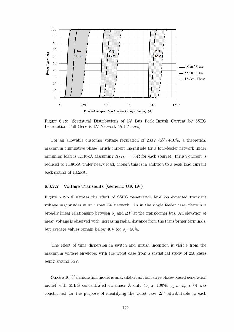
Figure 6.18: Statistical Distributions of LV Bus Peak Inrush Current by SSEGPenetration, Full Generic LV Network (All Phases)

For an allowable customer voltage regulation of 230V -6%/+10%, a theoretical

maximum cumulative phase inrush current magnitude for a four-feeder network under

minimum load is 1.316kA (assuming RLIM = 33Ω for each source). Inrush current is

reduced to 1.186kA under heavy load, though this is in addition to a peak load current

background of 1.02kA.

6.3.2.2 Voltage Transients (Generic UK LV)

Figure 6.19b illustrates the effect of SSEG penetration level on expected transient

voltage magnitudes in an urban LV network. As in the single feeder case, there is a

broadly linear relationship between ρg and ∆V at the transformer bus. An elevation of

mean voltage is observed with increasing radial distance from the transformer terminals,

but average values remain below 40V for ρg=50%.

The effect of time dispersion in switch and inrush inception is visible from the

maximum voltage envelope, with the worst case from a statistical study of 250 cases

being around 55V.

Since a 100% penetration model is unavailable, an indicative phase-biased generation

model with SSEG concentrated on phase A only (ρg A=100%, ρg B=ρg B=0) was

constructed for the purpose of identifying the worst case ∆V attributable to each

192

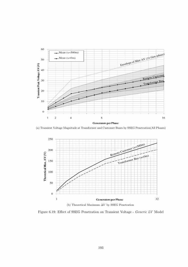
(a) Transient Voltage Magnitude at Transformer and Customer Buses by SSEG Penetration(All Phases)

(b) Theoretical Maximum ∆V by SSEG Penetration

Figure 6.19: Effect of SSEG Penetration on Transient Voltage - Generic LV Model

193

penetration scenario. The results of this model are depicted in Figure 6.19b, indicating

a theoretical maximum consumer bus ∆V of 230V under a 100% ρg scenario. This is

reduced to approximately 160V for ρg=50%, a roughly three-fold increase relative to

the upper ∆V envelope of Figure 6.19a. Dispersion of θi can, therefore, be said to have

a greater limiting effect on transient voltage magnitude as the extent of the simulation

network increases.

Feeder voltage magnitude profiles for the generic LV network are shown in Figure

6.20a for two ρg scenarios (12.5 and 50%). Continuing the trend of the single feeder

model, the peak voltages observed along the main LV trunk are nearly constant as

the cable impedance is inversely related to its current handling capacity. This may

be contrasted with the linearly position-dependent voltage profile associated with an

individual generator - see Chapter 5 (Section 5.4.1). Some attenuation is observed,

however, across the single phase service cable between consumer and adjacent LV node

(last 50m).

Figure 6.20b in turn depicts the theoretical maximum voltage profiles generated

from a coincident timed switch model (θi = 90). As with the single phase feeder

model, it is anticipated that field testing on a real network will generate ∆V profiles

lying between the values of Figures 6.20a and 6.20b.

194

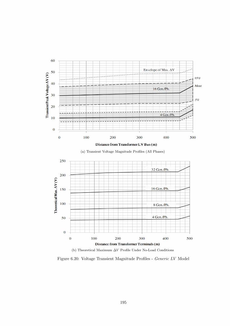
(a) Transient Voltage Magnitude Profiles (All Phases)

(b) Theoretical Maximum ∆V Profile Under No-Load Conditions

Figure 6.20: Voltage Transient Magnitude Profiles - Generic LV Model

195

6.3.3 Rural LV Feeder

A number of distinctions have been observed between transient propagation characteristics

in the urban and rural networks. A discussion of results obtained with the single generic

rural feeder model follows.

6.3.3.1 Current Transients (Rural)

Cumulative phase current distributions as measured at the LV transformer terminals

are consistent with those of the single urban feeder model. A minor reduction in

peak current and narrowing of the current range at full load are both attributable to

the increased series impedance of the network relative to the urban case. Normal load

current amplitude for the full load case is indicated by the vertical dashed line of Figure

6.21.

Figure 6.21: Statistical Distributions of LV Bus Peak Inrush Current by SSEGPenetration, Rural Feeder (Per-Phase)

6.3.3.2 Voltage Transients (Rural)

Figure 6.22 shows how the concentration of embedded generation within a rural network

impacts upon expected voltage transient magnitudes at different feeder locations.

The first distinction between the rural and urban results is in the measurement

location giving rise to the worst case ∆V . In an urban network, the most severe

transient voltage magnitudes are observed at the remote customer bus. The rural

network by contrast gives rise to a maximum ∆V at the adjacent LV node (x=1400m),

196

Figure 6.22: Transient Voltage Magnitude at Transformer and Customer Buses as aFunction of SSEG Penetration, Rural Network (All Phases)

as is visible from Figures 6.23a and 6.23b.

Mean voltage transient magnitudes at the LV node are approximately 50V for 100%

ρg, approximately twice their equivalent values from the urban case. ∆V at the same

location for ρg=50% (16 generators/phase) is equivalent to that of the generic LV model

under the same penetration scenario.

Of note is the greatly reduced transient magnitude at the transformer terminals. It

is clear that attenuation of SSEG-induced switching transients is greater in the overhead

rural circuit than in the underground urban network, due to the combined increase in

length and series impedance of the 230V circuit. The highest ∆V values are, therefore,

confined to the more remote rural nodes. This behaviour may also be partly attributed

to the elevated capacitance of underground circuits, though this effect is only marginal

as insulated aerial bundled conductors themselves are highly capacitance compared

with separated conductors.

The statistical and theoretical maximum ∆V profiles, of Figures 6.23a and 6.23b

respectively, indicate that a worst case transient magnitude of 240V occurs at a remote

LV node under a 100% SSEG penetration. This is to be contrasted with a 120V

maximum observed in the urban feeder model, suggesting that generators switching

under ER G83-1 [5] have a greater electromagnetic transient impact on rural feeders

197

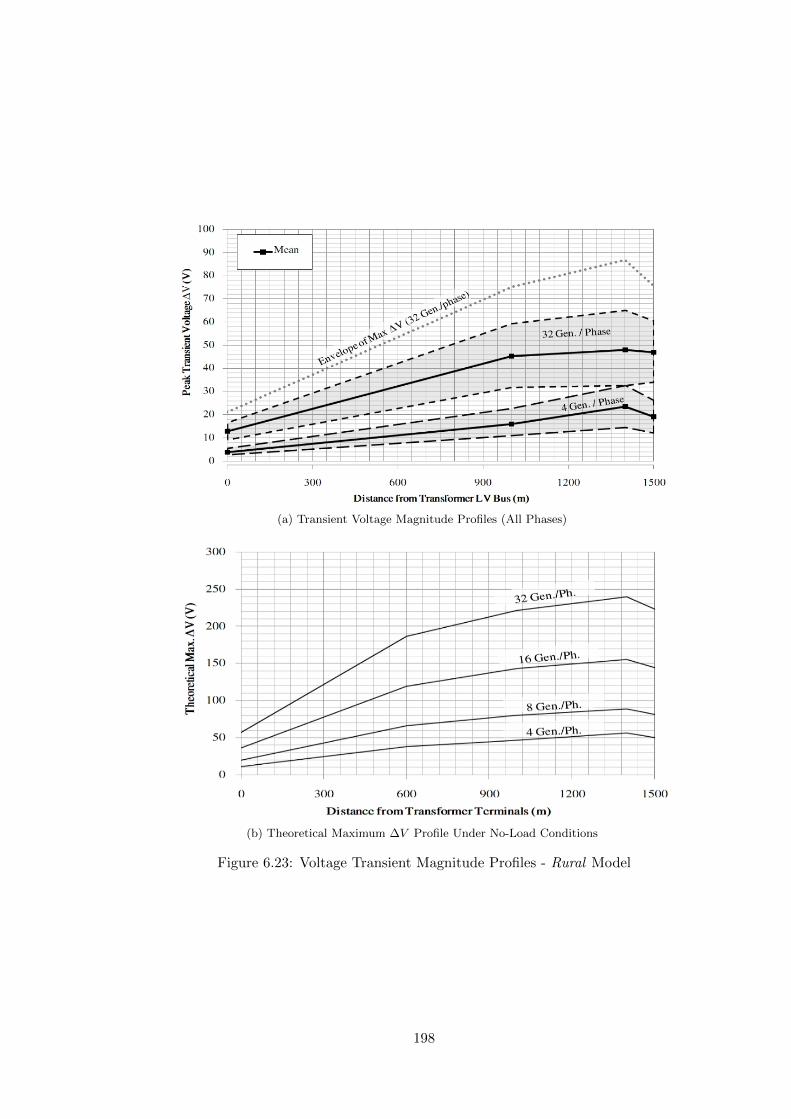
(a) Transient Voltage Magnitude Profiles (All Phases)

(b) Theoretical Maximum ∆V Profile Under No-Load Conditions

Figure 6.23: Voltage Transient Magnitude Profiles - Rural Model

198

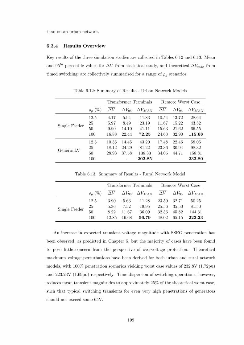
than on an urban network.

6.3.4 Results Overview

Key results of the three simulation studies are collected in Tables 6.12 and 6.13. Mean

and 95th percentile values for ∆V from statistical study, and theoretical ∆Vmax from

timed switching, are collectively summarised for a range of ρg scenarios.

Table 6.12: Summary of Results - Urban Network Models

Transformer Terminals Remote Worst Case

ρg (%) ∆V ∆V95 ∆VMAX ∆V ∆V95 ∆VMAX

Single Feeder

12.5 4.17 5.94 11.83 10.54 13.72 28.6425 5.97 8.49 23.19 11.67 15.22 43.5250 9.90 14.10 41.11 15.63 21.62 66.55100 16.88 22.44 72.25 24.63 32.90 115.68

Generic LV

12.5 10.35 14.45 43.20 17.48 22.46 58.0525 18.12 24.29 81.22 23.36 30.94 98.3250 28.93 37.58 138.33 34.05 44.71 158.81100 - - 202.85 - - 232.80

Table 6.13: Summary of Results - Rural Network Model

Transformer Terminals Remote Worst Case

ρg (%) ∆V ∆V95 ∆VMAX ∆V ∆V95 ∆VMAX

Single Feeder

12.5 3.90 5.63 11.28 23.59 32.71 50.2525 5.36 7.52 19.95 25.56 35.50 81.5050 8.22 11.67 36.09 32.56 45.82 144.31100 12.85 16.68 56.79 48.02 65.15 223.23

An increase in expected transient voltage magnitude with SSEG penetration has

been observed, as predicted in Chapter 5, but the majority of cases have been found

to pose little concern from the perspective of overvoltage protection. Theoretical

maximum voltage perturbations have been derived for both urban and rural network

models, with 100% penetration scenarios yielding worst case values of 232.8V (1.72pu)

and 223.23V (1.69pu) respectively. Time-dispersion of switching operations, however,

reduces mean transient magnitudes to approximately 25% of the theoretical worst case,

such that typical switching transients for even very high penetrations of generators

should not exceed some 65V.

199

At this voltage level, transients due to generator switching would be indistinguishable

from the regularly occurring low-magnitude background perturbations recorded by Bull

[80] and Goedbloed [81] (see Figure 1.15 on p33). If, as predicted, the frequency of

disconnection events was to rise along with SSEG penetration, there would likely be

some cause for concern regarding power quality and insulation degradation due to

frequently occurring low-magnitude, fast-front switching transients. This aspect shall

require further study in order to make any definite conclusions.

6.4 Scenario Probability

The probability that any of the simulated scenarios shall be encountered in practice is

of course dependent on the speed with which each generator responds to detection of

an abnormal system condition. Engineering recommendation G83-1 [5] requires that

generators disconnect within 1 second of over/under-voltage detection (0.5 seconds

in the case of over/under-frequency and/or loss of mains). It is anticipated that

all generators shall disconnect in a time well within these limits, and a Gaussian

distribution of disconnection times is assumed.

If all generators subsequently undergo a homogeneously specified grid monitoring

procedure, reconnection times shall occupy a similar distribution, though discretised

into 20ms segments by successive positive zero-crossings of the terminal voltage. The

number of concurrent switching events on each cycle shall then be proportional to the

normalised area under the continuous probability curve for the duration of that cycle.

An example is depicted in Figure 6.24 for a group of generators disconencting with a

mean time of 250ms, and a standard deviation of pole opening instants of 50ms.

Reconnection occurs after a grid-monitoring time τG (assuming that by this time

normal voltage/frequency conditions have been resumed), giving rise to the discretised

switch distribution on the right hand side. In this case, the maximum proportion of

generators switching on the same cycle (effective penetration, ρeff ) should be reduced

to approximately 16% of the total penetration.

Taking as an example the 100% penetration scenario in the Generic LV Model,

the effective penetration due to such switching characteristics would be reduced from

200

Figure 6.24: Probability of Coincident Switching for a Group of Generators

32 generators per feeder phase to only 5, and in such case the appropriate simulation

results for a lower ρg shall apply. Though this does not rule out coincident switching

of all generators, the probability of such an event is significantly reduced, depending

on the switching characteristics of each generator.

Table 6.14 summarises the effective penetration ρeff reconnecting on a single cycle

for a group of generators, based on the standard deviation of pole opening times.

Table 6.14: Proportion of Generator Group Switching on One Cycle

σsw (ms) 20 50 100

Effective Penetration on Median Cycle(%) 35 16 8

6.5 Options for Mitigation

Where switching transients are deemed to problems on LV networks from the perspective

of either insulation coordination or power quality. the most obvious course of action is

to prevent a high-coincidence scenario by manipulation of the grid monitoring delay τG.

Factory specification of grid inverters shall normally fix τG to 180 seconds as per

general recommendations in the connection standards [5, 6], which is unlikely to be

changed after installation in a customer’s premises. However the minimum allowable

τG for inverter based systems is 20s, and the author proposes that new installations

take advantage of this additional range so as to effect a dispersion of switching delays.

201

Adjustment to τG might either be made manually at the point of commissioning, or

automatically by means of a pseudo-random delay term generated on device firmware

installation.


Results of cumulative impact studies involving multiple spatially dispersed embedded

generators on an LV network have been presented. Key to the acquisition of these results

has been the development in EMTP-ATP of an extensive travelling wave equivalent of

the Generic LV Network model, as approved by UK DNOs. Smaller generic single-feeder

models have also been developed for high penetration studies relating to urban and rural

installations. It has been found that:

• LV networks incorporating up to 192 individually specified and spatially dispersed

embedded generators (50% of total households) may be modelled in detail in

EMTP for the purpose of systematic and statistical analyses while remaining

within the operational limits of the software;

• By treating embedded generation within a network on a per-phase basis, penetration

scenarios may be increased to 100% for the purpose of timed-switching (worst-case)

analyses;

• For the highest SSEG penetration scenarios, the theoretical maximum transient

voltage at the most remote point of the network due to mass reconnection of

generators is approximately 233V for the generic UK urban LV model (223V for

a rural feeder)

• Typical transient magnitudes at these locations are reduced to approximately 25%

of their theoretical maxima due to temporal dispersion of switch closing times and

inrush inception angles.

• Transient voltage peak values are attenuated to a greater degree in rural overhead

circuits than in urban underground cables, with simulated maximum amplitudes

at the LV transformer terminals dropping to 203V (urban) and 57V (rural).

• For lower penetrations of SSEG, there is little to distinguish the characteristics

of a typical cumulative transient event from the switching of a large load, thus

202

demanding little concern from the perspective of insulation coordination or EMC.

Statistical studies have revealed that time-dispersion between switch closing and

inrush inception instants of each generator significantly limits the magnitude of generated

transients, with mean voltage magnitudes at the customer bus and transformer terminals

reducing to 1.13 and 1.12 pu respectively for the generic UK LV network model. It is

hypothesised that these results may be conservative, due to overly randomised inrush

inception timing, and that true behaviour shall lie closer to the theoretical maxima. It

has been noted that diversity in the response times of grid disconnects serves to reduce

the effective penetration of coincidently switched generators.

As a general observation, Dommel’s EMTP method (using trapezoidal integration)

was found give a good balance between performance and solution speed for the large-scale

studies presented here. No significant problems were reported on the grounds of

solution stability or numerical oscillation. Some economy of model components might

be achieved in future, allowing for more extensive networks with higher SSEG penetrations

to be analysed using the same freely available software tools. At the present time, there

would appear to be no technical benefit in switching to alternative (Euler, Gear 2nd

Order, Runge-Kutta . . . ) or novel solution methods, though these options may be

exploited in future for verification purposes.

203

Conclusions

The primary focus of this thesis has been the development of models for the

computation of electromagnetic fast-transient propagation within LV networks,

and the application of said models in the context of an ever increasing penetration

of small embedded generators with ratings below 16 Amps per phase. This chapter

charts the most significant project findings and deliverables, and a number of ideas are

presented for further refinements and ongoing work.

As the gap between supply of and demand for electrical energy narrows, and concern

over climate change and primary fuel availability rises, there is an increasing need to

move towards a more distributed power generation model in order to accommodate the

necessary levels of renewable generation to meet long-term renewables and emissions

targets. With ever growing numbers of small generators feeding into public supply

networks, the consumer is set to play an increasingly active role in the energy market.

From the perspective of a network operator, however, there is little to distinguish

between a small generator rated at or below 16A per phase on the one hand and a

similarly rated load on the other. Indeed, the only distinction is in the direction of

real power flow and, for this reason, there is a tendency to regard such generators as

negative loads.

This designation at present precludes the use of such small scale embedded generation

for ancillary service provision, with a requirement instead that generators should disconnect

in response to excessive grid voltage or frequency deviation. It is hypothesised that as

the penetration of embedded generators on a given LV bus increases, these disconnection

requirements shall give rise to an increased incidence and severity of localised switching

transients on the 400/230V circuit above that already encountered. This thesis has

204

sought to predict the magnitudes of switching transients for a range of network topologies

and increasing SSEG penetration scenarios, and to propose options for mitigation in

cases where excessive voltages or currents are predicted.

Practical considerations pertinent to time-domain simulation of low-voltage networks

were first addressed including solution time-step limits imposed by short travelling wave

line segments and circuit time constants, and the need for an appropriate numerical

representation of compact non-circular conductor geometries. An evaluation of modal-

and phase-domain frequency dependent line models was undertaken, and found to yield

improved results over the simplified Π-equivalent employed in earlier work.

Generator switching patterns and associated transient characteristics were evaluated

from extensive testing of a photovoltaic inverter rig within the Cardiff University Solar

Energy Laboratory. Statistical analyses of amplitudes, front/tail times, ramp rates and

energy measures were used to formulate a suite of easily synthesised representative test

waveforms suitable for application to future laboratory and field tests. It was found

that capacitive inrush gave rise to the worst case transient current magnitudes, and

that the depth of voltage perturbations is heavily dependent on the impedance of the

LV circuit. Timing data of relay pole closing instants and inrush inception with respect

to the supply voltage sinusoid was used to specify statistical rules for the control of

switches in complex simulation models.

A trio of alternative source representations of varying complexity was developed

in EMTP-ATP for modelling transient behaviour associated with a range of switching

operations. The most versatile of these models incorporates an explicit representation

of the inverter DC bus and power electronic circuitry, and allows both disconnect and

reconnect operations to be investigated using a single model. The provision of such

flexibility, however, comes at the expense of solution accuracy, and a sensitivity to

initial conditions makes complex source representation undesirable for large studies.

Having determined experimentally that it is the generator reconnection process that

gives rise to the most significant transient voltages and currents, it was possible to adopt

a far simpler and more efficient reconnection-only model for the most computationally

demanding cumulative impact studies. This was a major benefit as the very largest

205

system studies undertaken required such extensive models that exhaustion of simulation

component limits was a frequent occurrence.

Indicative LV network feeder models were developed for fast transient analysis

from existing dynamic system studies and DNO planning guidelines. Indeed, the

primary novelty of this work has been the formulation of a detailed travelling wave

equivalent of the generic UK LV Network model, as recognised by the UK Distribution

Network Operators. It is intended that the developed model should remain useful for

studies beyond the scope of this document. The display limitations of the ATPDraw

preprocessor have been adhered to in order to maximise ease of use, and solution times

of 250-case statistical studies vary by complexity between 10 and 72 hours for a typical

modern workstation (2.8GHz dual core, 3GB RAM).

For the purpose of the cumulative studies, both generator penetration and aggregated

background load were assumed to have an even phase distribution and geographical

dispersion, with a discrete set of fixed scenarios proposed. Such an assumption was

deemed appropriate to the needs of this work, in order that the initial number of

variables be manageable. It is anticipated that more realistic diversity and imbalance

scenarios shall be incorporated into future studies.

Extensive simulations involving the generic UK LV network equivalent and rural

feeder models indicate absolute worst case maximum transient voltage magnitudes at

any location in the region of 233V and 223V respectively, for a 100% penetration

scenario in which each and every customer has some form of converter-interfaced

generating equipment, be it a PV system, micro CHP unit or small wind turbine.

A broadly linear relationship is found to exist between SSEG penetration and typical

transient voltage magnitudes, but some plateauing of maximum theoretical values is

observed due to partial voltage collapse on current inrush.

Time dispersion of switch pole closing and inrush inception, according to the statistical

behaviour determined from laboratory tests, was found to limit the severity of transients,

and envelopes of maximum voltage spike amplitudes were found to drop to around

35-40% of their theoretical maxima. It has been postulated that these results are

somewhat conservative, as in practice the diversity of inrush inception across a population

206

of generators should be constrained according to the charge states of each inverter’s

DC bus capacitance. Though highly variable from one switching event to the next,

variation between sources for the same event is likely to be minimal.

Regardless of such conservative statistical results, worst-case voltages and currents

are found to be more than manageable from the general perspective of insulation

coordination. There remains, however, the secondary consideration of electromagnetic

compatibility and received power quality, which must be addressed on a case by case

basis. A method for the artificial dispersion of switch timing by implementation of a

pseudorandom grid-monitoring delay has been proposed.

Suggestions for Future Work

Generic LV Model: Further Development

As discussed in Chapter 6, some difficulty was encountered in statistical representation

of very high SSEG penetration scenarios using the generic UK LV model, due to an

exhaustion of allowable network object counts. Efforts are ongoing to identify economies

that will in future work allow all possible penetration scenarios to be considered.

The limitation of the LCC routine with regard to handling of sectored conductors

is identified as a possible source of error in simulations of LV networks. It is proposed

that a finite-element frequency scan preprocessing stage be integrated into the cable

geometry specification for future studies, in place of the existing method in which

equivalent circular conductors are assumed and satisfaction of the assumptions of

Carson’s equations and correction factors cannot be guaranteed.

Consideration of Load/Generator Diversity

It is proposed that ongoing simulation studies using these updated models should also

account for diversity of instantaneous power demand by incorporating a variety of

customer load profiles, and giving consideration to the effect of load/generation phase

imbalance. Both of these aspects may be investigated with minimal adjustment to the

existing models.

207

Disconnection Frequency Sensitivity Analysis

It is proposed that a study be undertaken to quantify the expected frequency of

disconnection events for a typical grouping of generators on an LV feeder, and how

the size of a given generator group can be expected to impact this frequency. The

cascading effect of undervoltage protection relays under heavy load conditions is of

particular interest, as this is the most likely cause of simultaneous switching.

Field Study on a Real LV Feeder

Field measurements are proposed in order to confirm a number of this work’s assertions

- principally that inrush diversity across a generator group shall in practice be lower

than that assumed here, resulting in an increase of typical transient current and voltage

magnitudes. Since such a study would necessitate consideration of high SSEG feeder

penetrations, appropriate test networks would likely be limited to suburban housing

developments in which embedded generation has been installed at the time of construction.

Failing this, a representative laboratory based feeder model employing multiple inverters

could be constructed for the purpose of verifying statistically determined switching

behaviour.

Such a field study would also allow the simulation models presented in this thesis

to be developed from generic network approximations to true system representations in

which a real circuit topology is explicitly represented. Such an approach would permit

investigation of the effects of network topology on the frequency and severity of the

generated transients.

208

References

[1] “The growth potential for microgeneration in England, Wales and Scotland -report by Element Energy Ltd to BERR,” Department for Business Enterpriseand Regulatory Reform, Tech. Rep., 2008.

[2] M. Landy, “Analysis of renewables growth to 2020 - report to DECC,” AEATechnology, Tech. Rep., 2010.

[3] “Investigation into the Scope for the Transport Sector to Switch to ElectricVehicles and Plugin Hybrid Vehicles - Report by ARUP to BERR,” Departmentfor Busiess Enterprise and Regulatory Reform: Department of Transport, Tech.Rep., 2008.

[4] M. F. McGranaghan, R. M. Zavadil, G. Hensley, T. Singh, and M. Samotyj,“Impact of utility switched capacitors on customer systems: Magnification atlow voltage capacitors,” in Proceedings of the IEEE Power Engineering SocietyTransmission and Distribution Conference - Dallas, TX, 1991, pp. 908–914.

[5] Engineering Recommendation G83/1 - Recommendations for the Connection ofSmall-Scale Embedded Generators (Up to 16A Per Phase) in Parallel with PublicLow-Voltage Distribution Networks, Energy Networks Association Std., 2003.

[6] BS EN 50438:2007 - Requirements for the Connection of Micro-generators inParallel with the Public Low-voltage Distribution Network, British StandardsInstitution Std., 2007.

[7] Vision and Strategy for Europe’s Electricity Grids of the Future - EuropeanSmartGrids Technology Platform. Office for Official Publications of the EuropeanCommunities, 2006.

[8] Strategic Research Agenda for Europe’s Electricity Networks of the Future -European SmartGrids Technology Platform. Office for Official Publications ofthe European Communities, 2007.

[9] J. Watson, A. S. Bahaj, and P. A. James, “Unlocking the power house - innovationbrief,” Sussex Energy Group, SPRU, University of Sussex; Sustainable EnergyResearch Group, School of Civil Engineering and the Environment, University ofSouthampton, Tech. Rep., 2006.

[10] Renewable Energy Route Map for Wales. Welsh Government, 2008.

[11] Microgeneration Action Plan for Wales. Welsh Government, 2007.

[12] “Potential for microgeneration - study and analysis (final report),” Energy SavingTrust, Econnect and Element Energy, Tech. Rep., 2005.

209

[13] Microgeneration Strategy. Department for Energy and Climate Change (DECC),2011.

[14] Microgeneration Government-Industry Group Action Plan. Energy EfficiencyPartnership for Homes, 2011.

[15] J. Watson, R. Sauter, P. A. James, L. Myers, T. Venables, and R. Wing,“The regulatory impacts of domestic-scale microgeneration - response to Ofgemconsultation,” Sussex Energy Group, SPRU, University of Sussex; Dept. of Civiland Environmental Engineering, University of Southampton; Tanaka BusinessSchool, Dept. of Civil Engineering, Imperial College London, Tech. Rep., 2005.

[16] M. C. Claudy, C. Michelsen, and A. O’Driscoll, “The diffusion of microgenerationtechnologies - assessing the influence of perceived product characteristics on homeowners’ willingness to pay,” Energy Policy, vol. 39, no. 3, pp. 1459 – 1469, 2011.

[17] S. Ropenus, H. K. Jacobsen, and S. T. Schroder, “Network regulation and supportschemes - how policy interactions affect the integration of distributed generation,”Renewable Energy, vol. 36, no. 7, pp. 1949 – 1956, 2011.

[18] Energy Act 2004, Part 2; Sustainability and Renewable Energy Sources, Chapter1: Sustainable Energy, Section 82: ”Microgeneration”. UK Government.

[19] Connecting a Microgeneration System to a Domestic or Similar ElectricalInstallation (In parallel with mains supply). Electrical Safety Council, 2007.

[20] The Electricity Safety, Quality and Continuity Regulations 2002. UKGovernment - Crown Copyright, 2002.

[21] Engineering Recommendation G59/1 - Recommendations for the Connectionof Embedded Generation Plant to the Public Electricity Suppliers’ DistributionSystems, Energy Networks Association Std., 1991.

[22] P. Trichakis, P. C. Taylor, L. M. Cipcigan, P. F. Lyons, R. A. Hair, and T. Ma,“Aninvestigation of voltage unbalance in low voltage distribution networks with highlevels of SSEG,” in UPEC ’06: Proceedings of the 41st International UniversitiesPower Engineering Conference - Newcastle upon Tyne, UK, P. C. Taylor, Ed.,vol. 1, 2006, pp. 182–186.

[23] L. M. Cipcigan and P. C. Taylor, “Investigation of the reverse power flowrequirements of high penetrations of small-scale embedded generation,”RenewablePower Generation, IET, vol. 1, no. 3, pp. 160–166, 2007.

[24] L. M. Cipcigan, P. C. Taylor, and P. Trichakis, “The impact of small scale windgenerators on LV distribution system voltage,” in International Conference onClean Electrical Power (ICCEP) - Capri, Italy, 2007, pp. 9–13.

[25] P. Trichakis, P. C. Taylor, P. F. Lyons, and R. Hair, “Predicting the technicalimpacts of high levels of small-scale embedded generators on low voltagenetworks,” IET Renewable Power Generation, vol. 2, no. 4, pp. 249–262, 2008.

[26] Mott-Macdonald, “System integration of additional microgeneration (SIAM),”Department of Trade and Industry and Ofgem, Tech. Rep., June 2004.

210

[27] H. Perhad and B. Madden, “Numbers of microgeneration units installed inEngland, Wales, Scotland, and Northern Ireland - Final report for BERR,”Department for Busiess Enterprise and Regulatory Reform, Tech. Rep., 2008.

[28] C. McNaught and H. Haydock, “The AEA Microgeneration Index QuarterlySummary Report 1 (October),” AEA, Tech. Rep., 2010.

[29] C. McNaught and H. Haydock, “The AEA Microgeneration Index QuarterlySummary Report 2 (December),” AEA, Tech. Rep., 2010.

[30] R. Harper, “UK trends in microgeneration adoption,” RWE nPower, Tech. Rep.,2008.

[31] D. Infield and F. Li, “Integrating micro-generation and distribution systes - areview of recent research,” IEEE Power and Energy Society General Meeting:Conversion and Delivery of Electrical Energy in the 21st Century - Pittsburgh,PA, 2008.

[32] J. Harrison, “Micro combined heat and power,” EA Technology, Tech. Rep., 2003.

[33] P. F. Lyons, P. C. Taylor, L. M. Cipcigan, P. Trichakis, and A. Wilson, “Smallscale energy zones and the impacts of high concentrations of small scale embeddedgenerators,” in UPEC ’06. Proceedings of the 41st International UniversitiesPower Engineering Conference - Newcastle upon Tyne, UK, vol. 1, 2006, pp.128–132.

[34] C. McNaught and H. Haydock, “The AEA Microgeneration Index QuarterlySummary Report 3 (March),” AEA, Tech. Rep., 2011.

[35] Photovoltaics in Buildings: Guide to installation of PV Systems (2nd Edition).Depatment of Trade and Industry, 2006.

[36] Photovoltaic Module Datasheets for Systems up to 600V, SHARP, last accessdate: July 2011. [Online]. Available: http://www.sharpusa.com/SolarElectricity/SolarProducts/LiteratureDownloads.aspx

[37] Photovoltaic Module Datasheets for Systems up to 600V, BPSolar, last access date:August 2011. [Online]. Available: http://www.bp.com/sectiongenericarticle.do?categoryId=9019590&contentId=7036980

[38] RenSMART. (2011) PV comparison table. Last access date: July 2011. [Online].Available: http://www.rensmart.com/Products/SolarPV

[39] R. Ramakumar and J. E. Bigger,“Photovoltaic systems,”Proceedings of the IEEE,vol. 81, no. 3, pp. 365–377, 1993.

[40] K. Akhmad, F. Belley, A. Kitamura, F. Yamamoto, S. Akita, H. Takakura,H. Okamoto, and Y. Hamakawa, “Effect of installation conditions on the outputcharacteristics of photovoltaic modules,” in First IEEE World Conference onPhotovoltaic Energy Conversion; Twenty Fourth IEEE Photovoltaic SpecialistsConference - Waikoloa, Hawaii, vol. 1, 1994, pp. 730–733.

[41] G. Sinden, “Wind power and the UK wind resource,” Environmental ChangeInstitute, University of Oxford, Tech. Rep., 2005.

211

http://www.sharpusa.com/SolarElectricity/SolarProducts/LiteratureDownloads.aspx

http://www.sharpusa.com/SolarElectricity/SolarProducts/LiteratureDownloads.aspx

http://www.bp.com/sectiongenericarticle.do?categoryId=9019590&contentId=7036980

http://www.bp.com/sectiongenericarticle.do?categoryId=9019590&contentId=7036980

http://www.rensmart.com/Products/SolarPV

[42] Installing small wind-powered electricity generating systems. Energy SavingTrust - Energy Efficiency Best Practice in Housing, 2004.

[43] A. Mirecki, X. Roboam, and F. Richardeau, “Architecture complexity and energyefficiency of small wind turbines,” Industrial Electronics, IEEE Transactions on,vol. 54, no. 1, pp. 660–670, 2007.

[44] “Domestic roof-mounted wind turbines - the current state of the art,” Mid WalesEnergy Agency, Tech. Rep., 2005.

[45] S. J. Watson. (2007) Predicting the yield of micro-wind turbines in theroof-top urban environment. Centre for Renewable Energy Systems Technology(CREST), Loughborough University. Last access date: July 2011. [Online].Available: http://www.warwickwindtrials.org.uk/resources/Microwind.pdf

[46] G. Y. Pam and E. J. Bala, “Potential output power from the 20 kW jacobs windturbine generator across 19 sites in northern Nigeria,” in Proceeding of the 5thEuropean-African Conference on Wind Engineering (EACWE) - Florence, Italy,2009.

[47] Proven WT2500 2.5kW Wind Turbine Datasheet, Proven Engineering ProductsLtd, Wardhead Park, Stewarton, Ayrshire, KA3 5LH.

[48] A. Glass and G. Levermore, “Micro wind turbine performance under real weatherconditions in urban environment,” Building Services Engineering Research andTechnology, vol. 32, no. 3, pp. 245–262, August 2011.

[49] S. Turan, A. Peacock, and M. Newborough, “Micro and small wind turbineapplications in the built environment,” INESCO Science and Technology Vision,vol. 3, no. 3, pp. 106–110, 2007.

[50] R. Gross, G. Jenkins, O. Paish, B. W. Leyland, N. Eyre, J. Harrison,C. Mahkamov, K. andHurley, J. L. Slowe, B. WIlliams, R. Hacker, R. Heap,L. Magistry, and I. Burdon, Micro Energy Systems: Review of Technology, Issuesof Scale and Integration, M. Knowles, I. Burdon, and R. Beith, Eds. ProfessionalEngineering Publishing, 2004.

[51] R. Lasseter, A. Akhil, C. Marnay, J. Stevens, J. Dagle, R. Guttromson, A. S.Meliopoulos, R. Yinger, and J. Eto, “The CERTS Microgrid Concept - Whitepaper on Integration of Distributed Energy Sources,” 2002.

[52] N. Hatziargyriou, H. Asano, R. Iravani, and C. Marnay, “Microgrids,” Power andEnergy Magazine, IEEE, vol. 5, no. 4, pp. 78–94, 2007.

[53] C. Marnay and G. Venkataramanan, “Microgrids in the evolving electricitygeneration and delivery infrastructure,” in IEEE Power Engineering SocietyGeneral Meeting, 2006.

[54] (2012) Profile: Baxi ecogen micro-chp unit. The Combined Heat andPower Association. Last access date: February 2012. [Online]. Available:http://www.chpa.co.uk/micro-chp 190.html

[55] J. Harrison. (2012) Stirling engines. Last access date: July 2012. [Online].Available: http://www.microchap.info/stirling engine.htm

212

http://www.warwickwindtrials.org.uk/resources/Microwind.pdf

http://www.chpa.co.uk/micro-chp_190.html

http://www.microchap.info/stirling_engine.htm

[56] M. Pielke and M. Kurraat, “Integration of combined heat and power micro unitsinto the low voltage network by using a grid-oriented operation mode,” in CIREDSeminar 2008: SmartGrids for Distribution, Frankfurt, Germany, 2008.

[57] R. Jablko, C. Saniter, R. Hanitsch, and S. Holler, “Technical and economicalcomparison of micro CHP systems,” in International Conference on Future PowerSystems - Amsterdam, Netherlands, 2005, p. 6 pp.

[58] G. Meeks, D. Sowden, and C. Yates. (2012) Press release -industry welcomes forthcoming rise in feed-in tariff for microCHP.Combined Heat and Pwoer Association (CHPA). Last accessdate: February 2012. [Online]. Available: http://www.chpa.co.uk/industry-welcomes-forthcoming-rise-in-feed-in-tariff-for-microchp- 659.html

[59] R. Mallwitz and B. Engel, “Solar power inverters,” in 6th International Conferenceon Integrated Power Electronics Systems (CIPS), 2010, pp. 1 –7.

[60] J. A. Baroudi, V. Dinavahi, and A. M. Knight, “A review of power convertertopologies for wind generators,” Renewable Energy, vol. 32, no. 14, pp. 2369–2385,2007.

[61] A. S. Emhemed, R. M. Tumilty, G. M. Burt, and J. R. McDonald, “Transientperformance analysis of single-phase induction generators for microgenerationapplications,” in 4th IET Conference on Power Electronics, Machines and Drives(PEMD) - York, UK, 2008, pp. 345–349.

[62] P. Chiradeja and R. Ramakumar, “Voltage profile improvement with distributedwind turbine generation: A case study,” in IEEE Power Engineering SocietyGeneral Meeting - Totonto, Canada, vol. 4, 2003, p. 2336.

[63] P. Chiradeja and R. Ramakumar, “An approach to quantify the technical benefitsof distributed generation,” IEEE Transaction on Energy Conversion,, vol. 19,no. 4, pp. 764–773, 2004.

[64] T. Tran-Quoc, C. Andrieu, and N. Hadjsaid, “Technical impacts of smalldistributed generation units on LV networks,” in IEEE Power Engineering SocietyGeneral Meeting - Toronto, Canada, C. Andrieu, Ed., vol. 4, 2003, p. 2464.

[65] R. O’Gorman and M. A. Redfern, “The difficulties of connecting renewablegeneration into utility networks,” in IEEE Power Engineering Society GeneralMeeting - Toronto, Canada, vol. 3, 2003, p. 1471.

[66] N. Silva and G. Strbac, “Optimal design policy and strategic investment indistribution networks with distributed generation,” in CIRED Seminar: SmartGrids for Distribution - Frankfurt, Germany, 2008.

[67] M. Thomson and D. Infield, “Network power-flow analysis for a high penetrationof distributed generation,” IEEE Transactions on Power Systems, vol. 22, no. 3,pp. 1157 –1162, 2007.

[68] BS EN 50160:2007 - Voltage characteristics of electricity supplied by publicdistribution networks, British Standards Institute Std., 2007.

[69] S. Conti, S. Raiti, G. Tina, and U. Vagliasindi, “Distributed generation in LVdistribution networks: voltage and thermal constraints,” in Proceedings of theIEEE Power Tech Conference - Bologna, Italy, vol. 2, june 2003.

213

http://www.chpa.co.uk/industry-welcomes-forthcoming-rise-in-feed-in-tariff-for-microchp-_659.html

http://www.chpa.co.uk/industry-welcomes-forthcoming-rise-in-feed-in-tariff-for-microchp-_659.html

[70] G. Barwaldt and M. Kurrat, “Application of energy storage systems minimizingeffects of fluctuating feed-in of photovoltaic systems,” in CIRED Seminar: SmartGrids for Distribution - Frankfurt, Germany, 2008.

[71] S. Conti, S. Raiti, and G. Tina, “Small-scale embedded generation effecton voltage profile: an analytical method,” IEE Proceedings on Generation,Transmission and Distribution, vol. 150, no. 1, pp. 78 – 86, jan. 2003.

[72] S. Fletcher, K. Meah, and S. Ula, “Simulation and analysis of a solar photovoltaicgeneration system for voltage support in a distributed generation scheme,” inProceedings of the IEEE Region 5 Technical Conference - Fayetteville, AR.Institute of Electrical and Electronic Engineers, 2007.

[73] B. Renders, W. R. Ryckaert, K. De Gusseme, K. Stockman, and L. Vandevelde,“Improving the voltage dip immunity of converter-connected distributedgeneration units,” Renewable Energy, vol. 33, pp. 1011–1–18, 2008.

[74] R. Ramakumar and P. Chiradeja, “Distributed generation and renewable energysystems,” in IECEC ’02 - The 37th Intersociety Energy Conversion EngineeringConference - Washington, DC, 2002, pp. 716–724.

[75] P. Chiradeja, “Benefit of distributed generation: A line loss reduction analysis,”in IEEE/PES Transmission and Distribution Conference and Exhibition: Asiaand Pacific - Dalian, China, 2005, pp. 1–5.

[76] L. Tao, C. Schwaegerl, and N. Hermann, “Impact of microgrids concept on lowvoltage network reliability,” in CIRED Seminar: Smart Grids for Distribution -Frankfurt, Germany, 2008.

[77] A. Bhowmik, A. Maitra, S. M. Halpin, and J. E. Schatz, “Determination ofallowable penetration levels of distributed generation resources based on harmoniclimit consideration,” IEEE Power Engineering Review, vol. 22, no. 4, pp. 79–79,2002.

[78] L. Gertmar, P. Karlsson, and O. Samuelsson, “On DC injection to AC gridsfrom distributed generation,” in European Conference on Power Electronics andApplications - Dresden, Germany, 2005.

[79] Sunny Boy 700 - Technical Description. Solar Inverter for Photovoltaic Plants,1st ed., SMA Reglesysteme GmbH.

[80] J. Bull and W. Nethercot, “The frequency of occurrence and the magnitude ofshort duration transients in low-voltage supply mains,” Radio and ElectronicEngineer, vol. 28, no. 3, pp. 185 –190, 1964.

[81] J. Goedbloed, “Transients in low-voltage supply networks,” IEEE Transactionson Electromagnetic Compatibility, vol. 29, no. 2, pp. 104 –115, May 1987.

[82] W. Rhoades, “Congruence of low voltage power main transient designs,” in IEEENational Symposium on Electromagnetic Compatibility - Denver, CO, may. 1989,pp. 285 –293.

[83] A. Tjader and J. Daalder, “Transients due to load energizing in low voltagesystems,” in Proceedings of the 18th International Conference on ElectricityDistribution (CIRED) - Turin, Italy, 2005.

214

[84] D. Mansson, T. Nilsson, R. Thottappillil, and M. Backstrom, “Propagation ofUWB transients in low-voltage installation power cables,” IEEE Transactions onElectromagnetic Compatibility, vol. 49, no. 3, pp. 585 –592, 2007.

[85] D. Mansson, R. Thottappillil, and M. Backstrom, “Propagation ability ofUWB transients through junctions of low-voltage power installation cable,” inAsia-Pacific Symposium on Electromagnetic Compatibility and 19th InternationalZurich Symposium on Electromagnetic Compatibility - Singapore, May 2008, pp.279 –282.

[86] A. Ametani, K. Hashimoto, and N. Nagaoka, “Modeling of incoming lightningsurges into a house in a low-voltage distribution system,” EMTP Journal, vol. 11,2006.

[87] F. J. Pazos, J. Amantegui, F. Ferrandis, and A. Barona, “Overvoltages in lowvoltage systems due to normal medium voltage switching,” May 21-24 2007.

[88] I. Metwally and F. Heidler,“Influence of line routing and terminations on transientovervoltages in lv power installations,” in 18th International Zurich Symposiumon Electromagnetic Compatibility, sep. 2007, pp. 313 –316.

[89] P. Osmokrovic, B. Loncar, and S. Stankovic, “The new method of determiningcharacteristics of elements for overvoltage protection of low-voltage system,” IEEETransactions on Instrumentation and Measurement, vol. 55, no. 1, pp. 257–265,2006.

[90] D. Paul, “Low voltage power system surge overvoltage protection,” in IEEEIndustrial and Commercial Power Systems Technical Conference - ClearwaterBeach, FL, 2000, pp. 21–29.

[91] F. Fiamingo, M. Marzinotto, C. Mazzetti, Z. Flisowski, G. B. Lo Piparo, andG. L. Amicucci, “Evaluation of SPD protection distance in low-voltage systems,”Journal of Electrostatics, vol. 65, no. 5-6, pp. 363–370, 2007.

[92] F. Silva, S. Pinto, and J. Silva, “Impact of microgeneration on the quality ofpower: Effect on the voltage waveform,” in 35th Annual Conference of IndustrialElectronics (IECON) - Porto, Portugal, nov. 2009, pp. 3672 –3678.

[93] N. Tse and L. Zhou, “Detection of voltage variations due to distributed energyresources,” in IEEE Power Energy Society General Meeting, 2009, pp. 1 –5.

[94] F. Pazos and E. Navarro, “Field experience of power frequency overvoltagesin wide-scale photovoltaic systems,” in CIGRE/IEEE PES Joint Symposium:Integration of Wide-Scale Renewable Resources Into the Power Delivery System- Calgary, Canada, 2009, p. 1.

[95] A. Ametani, M. Kizilcay, M. P. Pereira, B. J. Elliott, W. S. Meyer, J. Choo,C. Huang, and W. Levy, Rule Book - Alternative Transients Program - Part I,1987.

[96] H. W. Dommel, “Digital computer solution of electromagnetic transients insingle-and multiphase networks,” IEEE Transactions on Power Apparatus andSystems, vol. PAS-88, no. 4, pp. 388–399, 1969.

215

[97] A. Ametani, M. Kizilcay, M. P. Pereira, B. J. Elliott, W. S. Meyer, J. Choo,C. Huang, and W. Levy, Rule Book - Alternative Transients Program - Part IV,1987.

[98] T. Noda and A. Ametani, User Instructions of Noda Setup in ATP, 1997.

[99] A. Ametani, M. Kizilcay, M. P. Pereira, B. J. Elliott, W. S. Meyer, J. Choo,C. Huang, and W. Levy, Rule Book - Alternative Transients Program - Part V,1987.

[100] A. Ametani, M. Kizilcay, M. P. Pereira, B. J. Elliott, W. S. Meyer, J. Choo,C. Huang, and W. Levy, Rule Book - Alternative Transients Program - Part III,1987.

[101] J. Martinez, J. Mahseredjian, and R. Walling, “Parameter determination:procedures for modeling system transients,” IEEE Power and Energy Magazine,vol. 3, no. 5, pp. 16 – 28, 2005.

[102] J. Martinez, B. Gustavsen, and D. Durbak, “Parameter determination formodeling system transients - part I: overhead lines,” IEEE Transactions on PowerDelivery, vol. 20, no. 3, pp. 2038 – 2044, 2005.

[103] B. Gustavsen, J. Martinez, and D. Durbak, “Parameter determination formodeling system transients-part II: Insulated cables,” IEEE Transactions onPower Delivery, vol. 20, no. 3, pp. 2045 – 2050, 2005.

[104] J. Martinez, R. Walling, B. Mork, J. Martin-Arnedo, and D. Durbak, “Parameterdetermination for modeling system transients-part III: Transformers,” IEEETransactions on Power Delivery, vol. 20, no. 3, pp. 2051 – 2062, july 2005.

[105] J. Martinez and D. Durbak, “Parameter determination for modeling systemstransients-part V: Surge arresters,” IEEE Transactions on Power Delivery,vol. 20, no. 3, pp. 2073 – 2078, july 2005.

[106] J. Martinez, J. Mahseredjian, and B. Khodabakhchian, “Parameter determinationfor modeling system transients-part VI: Circuit breakers,” IEEE Transactions onPower Delivery, vol. 20, no. 3, pp. 2079 – 2085, july 2005.

[107] B. Johnson, H. Hess, and J. Martinez, “Parameter determination for modelingsystem transients-part VII: Semiconductors,” IEEE Transactions on PowerDelivery, vol. 20, no. 3, pp. 2086 – 2094, july 2005.

[108] O. Hevia, “Alternative transients program - comparison of transmission linemodels.”

[109] T. Tran-Anh and P. Auriol, “Distribution network modelling for power linecommunication applications,” in International Symposium on Power LineCommunications and Its Applications, 2005.

[110] W. Scott-Meyer, T. Liu, and H. W. Dommel, The Electromagnetic TransientsProgram (EMTP) Theory Book. Bonneville Power Administration, Portland,Oregon, 1995.

[111] G. F. Moore, Ed., BICC Cables: Electric Cables Handbook. Blackwell Science,1997.

216

[112] D. da Silva, G. Fernandez, and R. Rivas, “Calculation of frequency-dependentparameters of pipe-type cables: Comparison of methods,” in TDC ’06. IEEE/PESTransmission Distribution Conference and Exposition: Latin America - Caracas,Venezuela, 2006, pp. 1 –6.

[113] G. T. Andreou, D. P. Labridis, and G. K. Papagiannis, “Modelling low voltagedistribution cables for powerline communications,” in Proceedings of the IEEEPower Tech Conference - Bologna, Italy, 2003.

[114] G. T. Andreou and D. P. Labridis, “Electrical parameters of low-voltage powerdistribution cables used for power-line communications,” IEEE Transactions onPower Delivery, vol. 22, no. 2, pp. 879 –886, april 2007.

[115] S. Matsuura, T. Noda, A. Asakawa, and S. Yokoyama, “EMTP modelling of adistribution line for lightning overvoltage studies,” in IPST07 - Proceedings of theInternational Conference on Power Systems Transients - Lyon, France, 2007.

[116] R. Keyhani and D. Birtwhistle, “Modelling high frequency signal propagation overlow voltage overhead distribution networks using EMTP,” in IEEE InternationalSymposium on Power Line Communications and its Applications - Orlando, FL,2006, pp. 80 –85.

[117] P. N. Mikropoulos, T. E. Tsovilis, Z. Politis, and A. G. Kagiannas, “Evaluationof fast-front overvoltages arising at a 20/0.4 kV distribution transformer,” in 7thMediterranean Conference and Exhibition on Power Generation, Transmission,Distribution and Energy Conversion (MedPower 2010) - Agia Napa, Cyprus, nov.2010, pp. 1 –6.

[118] A. Morched, J. Marti, and J. Ottevangers, “A high frequncy transformer model forthe EMTP,” IEEE Transactions on Power Delivery, vol. 8, no. 3, pp. 1615–1626,1993.

[119] C. Brozio and H. Vermeulen, “Wideband equivalent circuit modellingand parameter estimation methodology for two-winding transformers,” IEEProceedings on Generation, Transmission and Distribution, vol. 150, no. 4, pp.487 – 492, july 2003.

[120] PD IEC TR 60071-4:2004 - Insulation co-ordination, Part 4: Computationalguide to insulation co-ordination and modelling of electrical networks, BritishStandards Institution Std., 2004.

[121] A. Ametani, M. Kizilcay, M. P. Pereira, B. J. Elliott, W. S. Meyer, J. Choo,C. Huang, and W. Levy, Rule Book - Alternative Transients Program - Part IX,1987.

[122] C. Ramırez and P. A. Calva, “Simultaion of electric power circuit breakers in theemtp incorporating electric arc models: Alpplication to reactor bank switchingand short line fault,” in Annual Report Conference on Electrical Insulation andDielectric Phenomena, 2001.

[123] N. Watson and J. Arillaga, Power Systems Electromagnetic TransientsSimulation, 1st ed., ser. IET Power and Energy Series 39. The Institution ofEngineeering and Technology, London, UK, 2003.

217

[124] L. Cipcigan, P. C. Taylor, T. Funabashi, and P. F. Lyons, “Active voltage controlin small-scale energy zones,” Transactions of the Japanese Institute of ElectricalEngineer (IEEJ), vol. 124, pp. 1–10, 2004.

[125] J. J. Grainger and W. Stevenson, Power Systems Analysis, A. B. Akay andE. Castellano, Eds. London, UK: McGraw-Hill Inc, 1994.

[126] E. Peskin, Transient and Steady-State Analysis of Electrical Networks. D. VanNostrand Company (Canada) Ltd, 1961.

[127] L. Freris and D. Infield, Renewable Energy in Power Systems. John Wiley andSons, Ltd, 2008.

[128] L. Cipcigan, “Numerical oscillations in electromagnetic transients programs,”in 11th International Symposium on System Theory, Automation, Robotics,Computers, Informatics, Electronics and Instrumentation (SINTES) - Craiova,Romania, 2003.

[129] N. Chiesa and H. K. Høidalen, “On the calculation of fluxl inkage/current-characteristics for delta-coupled transformer windings.” EEUG - EuropeanEMTP User Group, 2005.

[130] T. Noda, N. Nagaoka, and A. Ametani, “Phase domain modeling offrequency-dependent transmission lines by means of an ARMA model,” IEEETransactions on Power Delivery, vol. 11, no. 1, pp. 401 –411, jan 1996.

[131] BS IEC 60287-1-1:2006 - Electric cables. Calculation of the current rating.Current rating equations (100% load factor) and calculation of losses. General,British Standards Institution Std., 31 January 2007 2006.

[132] W. Mingli and F. Yu, “Numerical calculations of internal impedance of solidand tubular cylindrical conductors under large parameters,” IEE Proceedings onGeneration, Transmission and Distribution, vol. 151, no. 1, pp. 67 – 72, January2004.

[133] BS 7870-3.40:2001 LV and MV polymeric insulated cables for use by distributionand generation utilities. Specification for distribution cables of rated voltage 0.6/1kV. XLPE insulated, copper wire waveform concentric cables with solid aluminiumconductors, British Standards Institution Std., 2001.

[134] BS 6004:2000 - Electric cables: PVC insulated, non-armoured cables for voltagesup to and including 450/750V, for electric power, lighting and internal wiring,British Standards Institution Std., 2000.

[135] BS 7870-3.10:2001, LV and MV polymeric insulated cables for use by distributionand generation utilities. Specification for distribution cables of rated voltage 0.6/1kV. PVC insulated combined neutral and earth copper wire concentric cables withcopper or aluminium conductors, British Standards Institution Std., 2001.

[136] BS 7870-3.20:2001 - LV and MV Polymeric Insulated Cables for use byDistribution and Generation Facilities - Part 3: Specification for DistributionCables of Rated Voltage 0.6/1 kV - Section 3.20: PVC Insulated Split ConcentricCables with Copper or Aluminium Conductors (Implementation of HD 603),British Standards Institution Std., 2001.

218

[137] BS EN 60664-1:2007 - Insulation coordination for equipment within low-voltagesystems, Part 1: Principles, requirements and tests, British Standards InstitutionStd., 2007.

[138] BS EN 60071-1:2006 - Insulation co-ordination, Part 1: Definitions, principlesand rules, British Standards Institution Std., 2006.

[139] BS 7870-5:2011 - LV and MV polymeric insulated cables for use by distributionand generation utilities Part 5: Polymeric insulated aerial bundled conductors(ABC) of rated voltage 0.6/1 kV for overhead distribution (Implementation ofHD 626), British Standards Institution Std., 2011.

[140] N. R. Watson, A. M. Cola, G. D. Irwin, and O. Nayak, “Z-domainfrequency-dependent network equivalent for electromagnetic transient studies,” inProceedings of the International Conference on Power Systems Transients (IPST)- Budapest, Hungary, 1999.

[141] Y. Wang and N. Watson, “Z-domain frequency-dependent AC-system equivalentfor electromagnetic transient simulation,” IEE Proceedings - Generation,Transmission and Distribution, vol. 150, no. 2, pp. 141–146, 2003.

[142] BS EN 60071-2:1997, IEC 60071-2:1996 Insulation co-ordination. Applicationguide, British Standards Institution Std., 1997.

[143] BS 6662:1985, IEC 60816:1984 - Guide to methods of measurement of shortduration transients on low voltage power and signal lines, British StandardsInstitution Std., 1985.

[144] BS EN 60904-3:2008 - Photovoltaic devices. Measurement principles forterrestrial photovoltaic (PV) solar devices with reference spectral irradiance data,BSi Std., 2008.

[145] BP 380 Datasheet - 80 Watt Photovoltaic Module: High-efficiency photovoltaicmodule using silicon nitride multicrystalline silicon cells, BP Solar, 2006.

[146] S. McFayden. (2012, June) Low-voltage fault tables. Myelectrical. Last accessdate: August 2012. [Online]. Available: http://myelectrical.com/notes/entryid/193/low-voltage-fault-tables

[147] D. Shchiff and R. D’Agostino, Practical Engineering Statistics. Wiley, New York,1996.

[148] BS EN 60060-1: 2010 - High-voltage test techniques, Part 1: General definitionsand test requirements, British Standards Institution Std.

[149] BS EN 61000-4-5:2006 - Electromagnetic compatibility (EMC). Testing andmeasurement techniques. Surge immunity test, British Standards Institution Std.,2006.

[150] M. Azab, “Improved circuit model of a photovoltaic array,” International Journalof Electrical Power and Energy Systems Engineering, vol. 2:3, 2009.

[151] D. Clark, A. Haddad, H. Griffiths, and N. N. Schulz, “Analysis of switchingtransients in domestic installations with grid-tied microgeneration,” in NorthAmerican Power Symposium (NAPS) - Starkville, MS, oct. 2009, pp. 1 –6.

219

http://myelectrical.com/notes/entryid/193/low-voltage-fault-tables

http://myelectrical.com/notes/entryid/193/low-voltage-fault-tables

[152] D. Clark, A. Haddad, and H. Griffiths, “Switching transient analysis ofsmall distributed generators in low voltage networks,” in CIRED 2009. 20thInternational Conference and Exhibition on Electricity Distribution - Prague,Czech Republic, june 2009, pp. 1 –4.

[153] A. Maknouninejad, N. Kutkut, and I. Batarseh, “Analysis and control of PVinverters operating in VAR mode at night,” in IEEE PES Innovative Smart GridTechnologies (ISGT) - Manchester, UK, 2011.

[154] BS EN 50525-1:2011 - Electric cables - Low voltage energy cables of rated voltagesup to and including 450/750 V. Part 1: General requirements, British StandardsInstitution Std.

[155] BS EN 50525-2-11:2011 - Electric cables. Low voltage energy cables of ratedvoltages up to and including 450/750V. Cables for general applications. Flexiblecables with thermoplastic PVC insulation, British Standards Institution Std.

[156] BS7671: Requirements for Electrical Installations - IEE Wiring Regulations 17thEdition, British Standards Institution Std., 2008.

[157] BS 7870-3.11:2001 - LV and MV polymeric insulated cables for use by distributionand generation utilities. Specification for distribution cables of rated voltage 0.6/1kV. XLPE insulated combined neutral and earth copper wire concentric cables withcopper or aluminium conductors (Implementation of HD 603), British StandardsInstitution Std., 2001.

[158] NSP/004/041 - Specification for LV ABC Overhead Lines, CE Electric UK Std.,January 2007.

[159] K. Brennan and M. Anderson. (2010) Consultation - reviewof typial domestic consumption values. Office of Gas andElectricity Markets (OFGEM). [Online]. Available: http://www.ofgem.gov.uk/Markets/RetMkts/Compl/Consumption/Documents1/Review%20of%20typical%20domestic%20consumption%20values.pdf

[160] A. Ametani, M. Kizilcay, M. P. Pereira, B. J. Elliott, W. S. Meyer, J. Choo,C. Huang, and W. Levy, Rule Book - Alternative Transients Program - PartsXVII-XVIII, 1987.

[161] B. Wareing, Wood Pole Overhead Lines, A. T. Johns and D. F. Warne, Eds. IETPower and Energy Series, 2005.

[162] Japanese atp user group secure server. Last access date: December 2011.[Online]. Available: thunderbird.kuee.kyoto-u.ac.jp

[163] European emtp user group secure server. Last access date: March 2012. [Online].Available: www.eeug.org

[164] B. Mork, R. Nelson, B. Kirkendall, and N. Stenvig, “Determination ofhigh-frequency current distribution using emtp-based transmission line modelswith resulting radiated electromagnetic fields,” in Proceedings of the IEEEInternational Symposium on Power Line Communications and its ApplicationsRio de Janeiro, Brazil, 2010.

220

http://www.ofgem.gov.uk/Markets/RetMkts/Compl/Consumption/Documents1/Review%20of%20typical%20domestic%20consumption%20values.pdf



thunderbird.kuee.kyoto-u.ac.jp

www.eeug.org

[165] A. Ametani, M. Kizilcay, M. P. Pereira, B. J. Elliott, W. S. Meyer, J. Choo,C. Huang, and W. Levy, Rule Book - Alternative Transients Program - Part VI,1987.

[166] V. Brandwajn, “Damping of numerical noise in the EMTP solution,” EMTPNewsletter, vol. 2, pp. 10–19, 1982.

[167] F. Alvarado, “Eliminating numerical oscillations in trapezoidal integration,”EMTP Newsletter, vol. 2, no. 3, pp. 20–32, 1982.

221

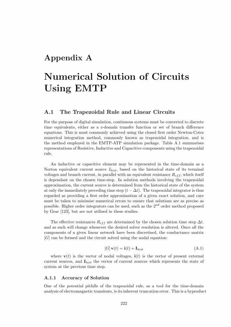
Appendix A

Numerical Solution of CircuitsUsing EMTP

A.1 The Trapezoidal Rule and Linear Circuits

For the purpose of digital simulation, continuous systems must be converted to discretetime equivalents, either as a z-domain transfer function or set of branch differenceequations. This is most commonly achieved using the closed first order Newton-Cotesnumerical integration method, commonly known as trapezoidal integration, and isthe method employed in the EMTP-ATP simulation package. Table A.1 summarisesrepresentations of Resistive, Inductive and Capacitive components using the trapezoidalrule.

An inductive or capacitive element may be represented in the time-domain as aNorton equivalent current source Ihist, based on the historical state of its terminalvoltages and branch current, in parallel with an equivalent resistance Reff , which itselfis dependant on the chosen time-step. In solution methods involving the trapezoidalapproximation, the current source is determined from the historical state of the systemat only the immediately preceding time step (t−∆t). The trapezoidal integrator is thusregarded as providing a first order approximation of a given exact solution, and caremust be taken to minimise numerical errors to ensure that solutions are as precise aspossible. Higher order integrators can be used, such as the 2nd order method proposedby Gear [123], but are not utilised in these studies.

The effective resistances Reff are determined by the chosen solution time step ∆t,and as such will change whenever the desired solver resolution is altered. Once all thecomponents of a given linear network have been discretised, the conductance matrix[G] can be formed and the circuit solved using the nodal equation:

[G] v(t) = i(t) + Ihist (A.1)

where v(t) is the vector of nodal voltages, i(t) is the vector of present externalcurrent sources, and Ihist the vector of current sources which represents the state ofsystem at the previous time step.

A.1.1 Accuracy of Solution

One of the potential pitfalls of the trapezoidal rule, as a tool for the time-domainanalysis of electromagnetic transients, is its inherent truncation error. This is a byproduct

222

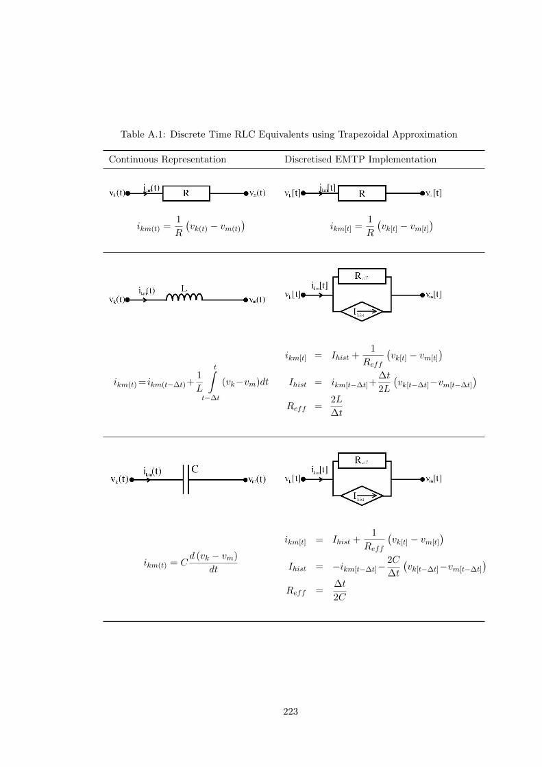
Table A.1: Discrete Time RLC Equivalents using Trapezoidal Approximation

Continuous Representation Discretised EMTP Implementation

ikm(t) =1

R

(vk(t) − vm(t)

)ikm[t] =

1

R

(vk[t] − vm[t]

)

ikm(t) = ikm(t−∆t)+1

L

t∫t−∆t

(vk−vm)dt

ikm[t] = Ihist +1

Reff

(vk[t] − vm[t]

)Ihist = ikm[t−∆t]+

∆t

2L

(vk[t−∆t]−vm[t−∆t]

)Reff =

2L

∆t

ikm(t) = Cd (vk − vm)

dt

ikm[t] = Ihist +1

Reff

(vk[t] − vm[t]

)Ihist = −ikm[t−∆t]−

2C

∆t

(vk[t−∆t]−vm[t−∆t]

)Reff =

∆t

2C

223

of its equivalence to a first-order approximate Taylor series expansion of the exponentialfunction. This is illustrated by analysis of the simple series RL branch of Figure A.1.

Figure A.1: Series RL Branch

Application of the trapezoidal rule in discretising this series arrangement results inthe difference equation (A.2) for the present state branch current [96,123]:

i[t] =

(1− ∆tR

2L

)(

1 +∆tR

2L

) i[t−∆t] +

∆t

2L(1 +

∆tR

2L

) (v[t] + v[t−∆t]) (A.2)

The exact analytical solution of the RL circuit current or central node voltage is afirst order exponential decay, while the difference equation defined from the trapezoidalrule is found by observation to be a combination of first order taylor series expansionsof the exact exponential:

e−x =e−

x2

ex2

'1− x

2+ · · ·

1 +x

2+ · · ·

(A.3)

where x =∆tR

L. This approximation results in a truncation error which is dependent

on the ratio of solution timestep and branch time constant. ∆t must, therefore,be carefully chosen to account for the shortest time constants and highest frequencycomponents in the system. It is preferable to select a value no greater than one thirdof the shortest time constant of the circuit [128] (τmin) in order that erroneous circuitbehaviour be avoided.

It is possible to minimise such errors through the use of exponential functions inthe system difference equations, thereby better approximating an analytical solution.This method is known as the Root Matching (Euler) approach, in that it exactly mapsthe roots of the frequency domain equivalent admittance matrix from the s- to thez-domain without the truncation error described above. There exist two variants ofthis method discussed later in the chapter.

A.1.2 Stability

Another point of note is the requirement that the digital solution be numerically stable.As already mentioned, the truncation error due to the trapezoidal approximation is afunction of the chosen simulation time step, and results in an imperfect mapping of thesystem transfer function from the continuous to the discrete time domain.

One important property of the trapezoidal rule, however, is that if the continuoustime transfer function of the network being modelled is stable, its mapping to thez-domain will always be stable [123]. This is a property not shared, for example, by

224

the more efficient forward Euler method and is one of the reasons that the EMTP(employing the trapezoidal integral) is the favoured solution method in this work.

It must be emphasised, however, that the stability of a solution does not implyits exactness, nor indeed vice versa. Certain circuit configurations involving minimallydamped RLC branches or short τ values are susceptible to marginal numerical stabilitywhen the trapezoidal rule is employed in its differential form. The result is typicallyan output that fluctuates alternately about the exact solution with each successivetime-step, known as Numerical Oscillation.

A.1.3 Numerical Oscillation

The effects of numerical oscillation are illustrated in Figure A.2. Here, a step responsehas been computed in EMTP-ATP for a simple RL circuit, with different ∆t - τ ratios.The damping factorK is the ratio of the parallel damping resistance Rp and the effectiveresistance of the inductive branch Reff .

K =RpReff

=Rp∆t

2L(A.4)

Figure A.2: Numerical Oscillation following current interruption in an RL circuit

It is clear from this example that the time-step must be well conditioned in orderto reflect the characteristics of the circuit, or the circuit suitably damped to relaxthe resolution requirement of low values of τ . This is a potentially resource-intensiverequirement in the simulation of low-voltage networks as individual component valuesare typically far smaller than their equivalents in high voltage systems for which theprogram was originally intended. This is a limiting consideration in the case of RCbranches where both values are likely to be very small.

The detrimental effects of numerical oscillation can be reduced with the conservativeapplication of damping resistance [110]. Where no existing stray or internal resistancecan be quantified in the real circuit being modelled, problematic LC components may bedamped by inclusion of fictitious resistances, placed either in parallel with inductancesor in series with capacitances. Employment of very short solver time steps (< 1µs)

225

will tend to increase the incidence of numerical oscillation as the gradients of currentand voltage discontinuities increases. The physical nature of Low-Voltage networkswill invariably demand time steps in the low nanosecond range, and as such dampingof numerical errors becomes increasingly important.

The choice of appropriate damping resistance is a compromise between maximisingthe rate of response, and minimising the introduction of phase errors in the solution[110], but the detrimental impact of artificial damping on the accurate representation ofa problem should always be considered. Table A.2 gives a range of recommended valuesfor damping resistances suitable for the treatment of spurious numerical oscillation inthe EMTP. The values preceding the effective resistance expressions are the dampingcoefficients Kp (parallel) and Ks (series) which can be modified within the EMTP.

Table A.2: Resistance Values for the Damping of Numerical Oscillation

Parallel Damping of an Inductor Series Damping of a Capacitor

Rp = Kp ·2L

∆t(5.4≤ Kp≤ 9.4) Rs = Ks ·

∆t

2C(0.1≤ Rs≤ 0.2) [166]

Rp =20

3· 2L

∆t[167]

The inclusion of damping resistance in parallel with the an inductor modifies theform of the branch difference equation of Table A.1. For a branch current i and voltdrop v :

v[t] =1

∆t

2L+

1

Rp

· (i[t]− i[t−∆t])− α · v[t−∆t] (A.5)

where α is the reciprocal of the damping factor:

α =Rp −

2L

∆t

Rp +2L

∆t

(A.6)

Numerical oscillation in the inductor voltage will, therefore, be damped for any valueof α less than 1. By setting the parallel resistance value equal to the effective resistanceof the inductor Reff , critical damping may be achieved, reducing the oscillation tozero in a single time step. This has the effect of removing the historic voltage termv[t − ∆t] from Equation (A.5), making the solution a function of present and pastbranch currents only. This critically damped case of the trapezoidal rule solution isknown as the backward Euler method, and is discussed alongside other alternativesin the next subsections. A similar result is obtained for the critical series damping ofoscillatory capacitor current.

226

A.1.4 Alternative Methods

The development of branch central difference equations by Dommel’s method is arguablythe most straightforward and flexible approach to the time-domain computation ofelectromagnetic transient phenomena. As discussed, however, this approach is proneto numerical oscillation when applied to simulations involving step voltages or currentinterruption [123]. An alternative to employing damping resistance in the EMTP is touse an exponential form of the branch difference equation. With reference to Equation(A.3), the expression derived by numerical integrator substitution for the current in aseries RL branch is in fact a truncated taylor series representation of the analyticallyexact exponential decay.

The error associated with this truncated form of the solution manifests itself in theimprecise mapping of system poles and zeros from the continuous s to the discrete zdomain - it is in fact the time-domain equivalent of the bilinear transform [123]. Errorscan be minimised by selecting a suitably short time step in relation to the branchtime constant, but this can give rise to excessively long simulation times when a farsmaller ∆t is required to satisfy the circuit characteristics than is needed to representthe highest frequency component of the transient. This requirement can be relaxed byextending the Taylor series to an infinitely large number of terms, thereby giving riseto the exponential form of the difference equation which is capable of computing exactsolutions regardless of the choice of time step. A desirable consequence of switching tothis method is the total elimination of spurious numerical oscillation, as it is in effecta critically damped trapezoidal rule solution.

The exponential form of the difference equation is known as the root-matchingmethod, because it eliminates the truncation error associated with the mapping ofroots from the s to z domain. Two frequently used forms of the root matching methodare the Forward and Reverse Rectangular (Euler) methods, as illustrated in Figure A.3.

Figure A.3: Rectangular and Trapezoidal Integrators

The use of a rectangular integrator has the effect of removing one term fromthe difference equation. For example, the voltage across an RL branch using theDommel method is dependent on the branch voltage and current at the previoustime step, and also the current at the present time. By contrast, the forward Eulermethod is dependent only on the past history terms v [t−∆t] and i [t−∆t], while thebackward Euler solution is independent of the historic voltage term v [t−∆t]. Thishas the effect of increasing the computation efficiency, but care must be taken with theforward rectangular method as the feed-forward nature of the solution makes it proneto instability.

227

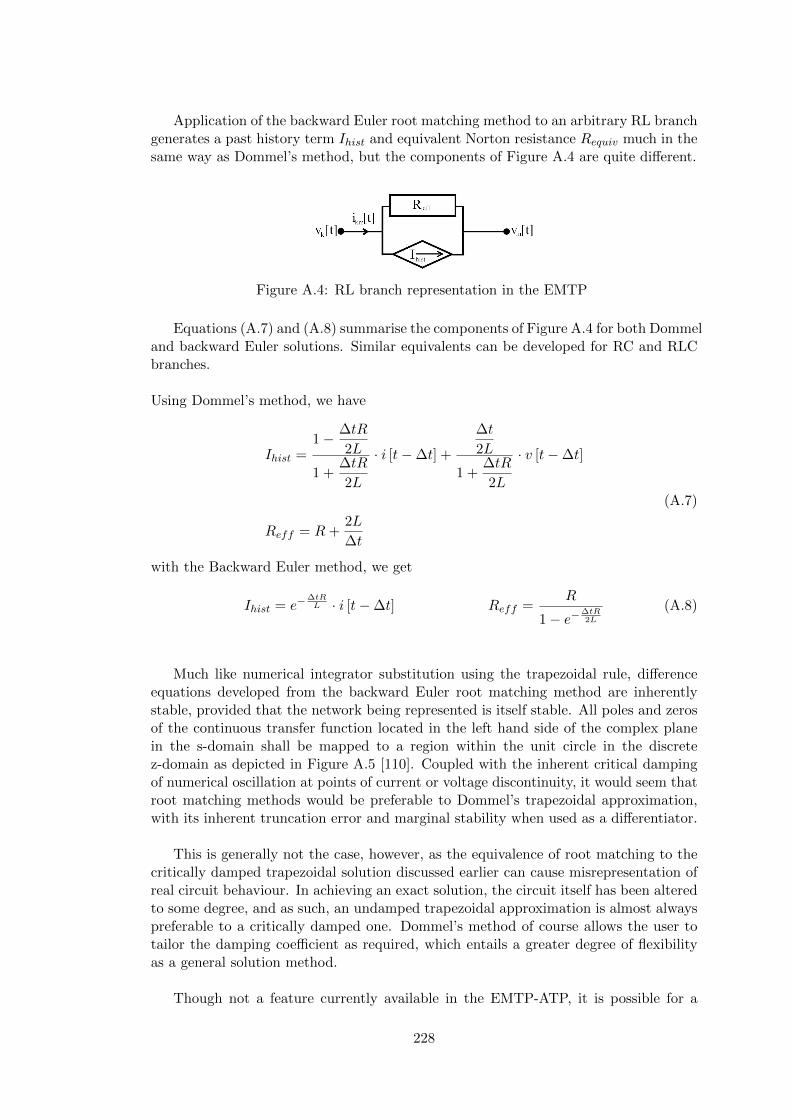
Application of the backward Euler root matching method to an arbitrary RL branchgenerates a past history term Ihist and equivalent Norton resistance Requiv much in thesame way as Dommel’s method, but the components of Figure A.4 are quite different.

Figure A.4: RL branch representation in the EMTP

Equations (A.7) and (A.8) summarise the components of Figure A.4 for both Dommeland backward Euler solutions. Similar equivalents can be developed for RC and RLCbranches.

Using Dommel’s method, we have

Ihist =1− ∆tR

2L

1 +∆tR

2L

· i [t−∆t] +

∆t

2L

1 +∆tR

2L

· v [t−∆t]

(A.7)

Reff = R+2L

∆t

with the Backward Euler method, we get

Ihist = e−∆tRL · i [t−∆t] Reff =

R

1− e−∆tR2L

(A.8)

Much like numerical integrator substitution using the trapezoidal rule, differenceequations developed from the backward Euler root matching method are inherentlystable, provided that the network being represented is itself stable. All poles and zerosof the continuous transfer function located in the left hand side of the complex planein the s-domain shall be mapped to a region within the unit circle in the discretez-domain as depicted in Figure A.5 [110]. Coupled with the inherent critical dampingof numerical oscillation at points of current or voltage discontinuity, it would seem thatroot matching methods would be preferable to Dommel’s trapezoidal approximation,with its inherent truncation error and marginal stability when used as a differentiator.

This is generally not the case, however, as the equivalence of root matching to thecritically damped trapezoidal solution discussed earlier can cause misrepresentation ofreal circuit behaviour. In achieving an exact solution, the circuit itself has been alteredto some degree, and as such, an undamped trapezoidal approximation is almost alwayspreferable to a critically damped one. Dommel’s method of course allows the user totailor the damping coefficient as required, which entails a greater degree of flexibilityas a general solution method.

Though not a feature currently available in the EMTP-ATP, it is possible for a

228

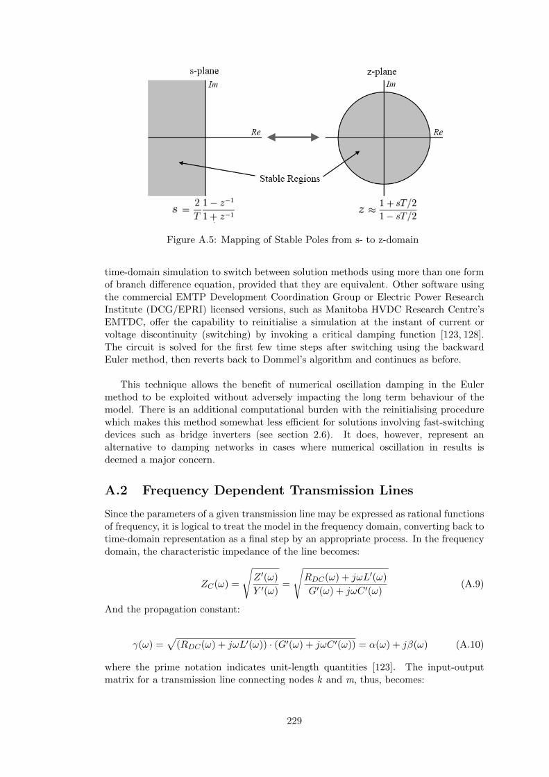
Figure A.5: Mapping of Stable Poles from s- to z-domain

time-domain simulation to switch between solution methods using more than one formof branch difference equation, provided that they are equivalent. Other software usingthe commercial EMTP Development Coordination Group or Electric Power ResearchInstitute (DCG/EPRI) licensed versions, such as Manitoba HVDC Research Centre’sEMTDC, offer the capability to reinitialise a simulation at the instant of current orvoltage discontinuity (switching) by invoking a critical damping function [123, 128].The circuit is solved for the first few time steps after switching using the backwardEuler method, then reverts back to Dommel’s algorithm and continues as before.

This technique allows the benefit of numerical oscillation damping in the Eulermethod to be exploited without adversely impacting the long term behaviour of themodel. There is an additional computational burden with the reinitialising procedurewhich makes this method somewhat less efficient for solutions involving fast-switchingdevices such as bridge inverters (see section 2.6). It does, however, represent analternative to damping networks in cases where numerical oscillation in results isdeemed a major concern.

A.2 Frequency Dependent Transmission Lines

Since the parameters of a given transmission line may be expressed as rational functionsof frequency, it is logical to treat the model in the frequency domain, converting back totime-domain representation as a final step by an appropriate process. In the frequencydomain, the characteristic impedance of the line becomes:

ZC(ω) =

√Z ′(ω)

Y ′(ω)=

√RDC(ω) + jωL′(ω)

G′(ω) + jωC ′(ω)(A.9)

And the propagation constant:

γ(ω) =√

(RDC(ω) + jωL′(ω)) · (G′(ω) + jωC ′(ω)) = α(ω) + jβ(ω) (A.10)

where the prime notation indicates unit-length quantities [123]. The input-outputmatrix for a transmission line connecting nodes k and m, thus, becomes:

229

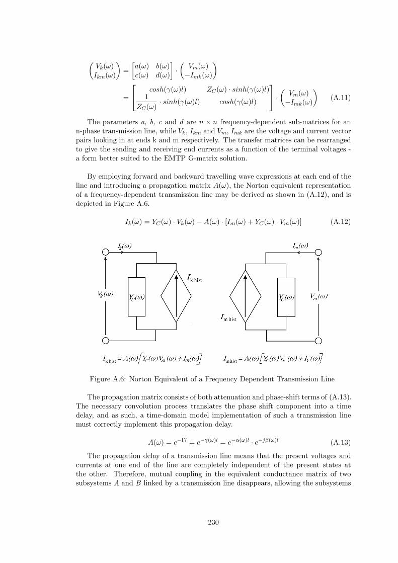
(Vk(ω)Ikm(ω)

)=

[a(ω) b(ω)c(ω) d(ω)

]·(Vm(ω)−Imk(ω)

)

=

cosh(γ(ω)l) ZC(ω) · sinh(γ(ω)l)1

ZC(ω)· sinh(γ(ω)l) cosh(γ(ω)l)

· ( Vm(ω)−Imk(ω)

)(A.11)

The parameters a, b, c and d are n × n frequency-dependent sub-matrices for ann-phase transmission line, while Vk, Ikm and Vm, Imk are the voltage and current vectorpairs looking in at ends k and m respectively. The transfer matrices can be rearrangedto give the sending and receiving end currents as a function of the terminal voltages -a form better suited to the EMTP G-matrix solution.

By employing forward and backward travelling wave expressions at each end of theline and introducing a propagation matrix A(ω), the Norton equivalent representationof a frequency-dependent transmission line may be derived as shown in (A.12), and isdepicted in Figure A.6.

Ik(ω) = YC(ω) · Vk(ω)−A(ω) · [Im(ω) + YC(ω) · Vm(ω)] (A.12)

Figure A.6: Norton Equivalent of a Frequency Dependent Transmission Line

The propagation matrix consists of both attenuation and phase-shift terms of (A.13).The necessary convolution process translates the phase shift component into a timedelay, and as such, a time-domain model implementation of such a transmission linemust correctly implement this propagation delay.

A(ω) = e−Γl = e−γ(ω)l = e−α(ω)l · e−jβ(ω)l (A.13)

The propagation delay of a transmission line means that the present voltages andcurrents at one end of the line are completely independent of the present states atthe other. Therefore, mutual coupling in the equivalent conductance matrix of twosubsystems A and B linked by a transmission line disappears, allowing the subsystems

230

to be represented as diagonal sub-matrices in [G]:

[G] =

[[GA]

[GB]

](A.14)

The increased sparsity of the conductance matrix arising from the use of transmissionline sections can greatly reduce the computational burden in simulating extensivemeshed networks. It is preferable to use a transmission line model in all cases, exceptthose in which it would itself impose prohibitively short ∆t requirements.

231

Appendix B

Laboratory Equipment and DAQ

B.1 Test and Measurement

Table B.1: Photovoltaic Test Rig Hardware

Mfr/Model Qty Description and Specification

BP380J 8 BPSolar Multicrystalline SiN PV ModuleNominal Power: 80W (±5%)Nominal Voltage: 12VVoltage at Pmax: 17.6VCurrent at Pmax: 4.55AShort Circuit Current: 4.80AOpen Circuit Voltage: 22.1VMax. System Voltage: 600V

SMA SB700 1 SMA SunnyBoy 700 Solar InverterInverter: Sine Wave, Current Source, 16kHz PWMSelected DC Input Range: <200VMax. DC Input Power: 670WNominal DC Bus Voltage: 125VMPP Voltage Range: 100-160VAC Nominal Power: 600WTHD: <3%Maximum Efficiency: 93.3%Certified Efficiency: 91.5%

WY NH204/63 1 Wylex 2 Way Consumer UnitMain DP Switch: 63ASingle Pole MCB: 16A

HA Birch B9427/2 1 Dummy Load - 0.4-31A

232

Tab

leB

.2:

Mea

sure

men

tan

dD

ata-

Acq

uis

itio

n(T

ran

sien

t)

Qty

Model

Des

crip

tion

Sp

ec.

1-

DA

QW

orkst

atio

nIn

tel

Cor

e2

E84

00(3

GH

z)4G

BR

AM

,W

indow

sX

PP

roSP

3

1L

eCro

yW

aver

unn

er64

Xi

600M

Hz

Osc

illo

scop

eB

andw

idth

:60

0MH

zB

WL

imit

:20

/200

MH

zC

han

nel

s:4

Inte

rlea

ved

Sam

ple

Rat

e:10G

S/s

Ver

tica

lR

esol

uti

on:

8b

it

2P

inte

kD

P25

Diff

eren

tial

Vol

tage

Pro

be

Ban

dw

idth

:25

MH

zC

MV

olta

ge:

1000

VA

Cpk

Att

enu

atio

n:

x20

,x50

,x200

Inp

ut

R:

4MΩ±

2%In

put

C:

1.2p

F±

5%

2T

ektr

onix

AM

503-

AC

urr

ent

Pro

be

Am

plifier

Ban

dw

idth

:D

C-

50M

Hz

2T

ektr

onix

A63

02C

urr

ent

Pro

be

Ban

dw

idth

:D

C-

50M

Hz

Curr

ent

Rat

ing:

20A

Conti

nu

ous

/50A

pk

233

Tab

leB

.3:

Mea

sure

men

tan

dD

ata-

Acq

uis

itio

n(S

tead

y-S

tate

)

Qty

Model

Des

crip

tion

Sp

ec.

1N

IU

SB

6212

Mu

ltif

un

ctio

nD

ata-

Acq

uis

itio

nB

oard

Res

oluti

on:

16b

itSam

ple

Rat

e:40

0kS

/s

Anal

ogue

IN(D

iff):

x8

Anal

ogue

OU

T:

x2

Dig

ital

I/O

:x32

1N

IG

PIB

-US

B-H

SN

atio

nal

Inst

rum

ents

GP

IBC

ontr

olle

r-

2L

eCro

yS

I900

0D

iffer

enti

alV

olta

geP

rob

eB

and

wid

th:

DC

-15M

Hz

Inp

ut

Z:

2MΩ

Att

enu

atio

n:

x20

,x200

CM

RR

(dB

,50

Hz)

:-8

0M

axim

um

Vol

tage

(diff

):±

700V

3L

EM

PR

20A

C/D

CC

urr

ent

Pro

be

Ban

dw

idth

:D

C-

20kH

zC

urr

ent

Ran

ge:±

30A

Wor

kin

gV

olta

ge:

300V

rms

1K

eith

ley

2000

Mult

imet

erB

andw

idth

:3H

z-

300kH

zIn

put

Z:

1MΩ±

2%

,100pF

Max

Vol

tage

:10

00V

pk

234

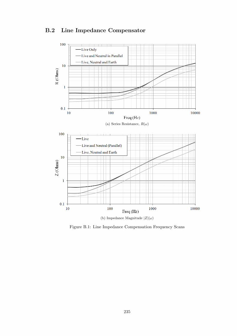
B.2 Line Impedance Compensator

(a) Series Resistance, R(ω)

(b) Impedance Magnitude |Z|(ω)

Figure B.1: Line Impedance Compensation Frequency Scans

235

Fig

ure

B.2

:L

abV

IEW

Dat

aL

ogge

r-

Blo

ckD

iagr

am

236

With reference to the LabVIEW block diagram in figure B.2, a breakdown of theindividual sub-vi components and their functions follows:

ScopeInit.vi is run as the first step of each test. It starts by fullyresetting the scope to a default configuration, and then sets eachmeasurement parameter in sequence according to the user inputs. Thisfunction is time-consuming at around 10 seconds, but is only performedonce per test as it is assumed that the same setup parameters are

required for each event in a particular test. The only additional scope setup requirementis the re-arming of the trigger between events which can be performed much moreefficiently by a second vi.

ScopeReset.vi allows the user to re-arm the trigger between events.This is achieved by adjusting the trigger from Stop to Auto and back toSingle with a time delay suitable to allow the scope to cycle fully. Sincethis does not require a complete scope reset, the process is much fasterthan the initial setup, and the program need only pass the original

trigger setup values to this vi.

AcquireData.vi takes a snapshot of the steady-state voltages andcurrents in the system with a sampling rate and duration defined in theinitial test setup. Quantities to monitor are extracted via predefinedglobal channels, and scaled according to the user-input scaling factors(e.g. the attenuation of the probes used). The scaled signals are

combined in a dynamic data cluster, and triggered relative to a rising edge of theAC voltage cycle to maintain a stable display.

SSDataProcess.vi takes the dynamic data cluster output from theprevious vi, and performs a set of statistical tests to extract informationabout the present steady-state of the system. The vi returns mean DCvoltage and current, and both peak and rms AC voltage and currentfor each successive snapshot.

PowerAnalysis.vi takes the same data cluster, and applies a poweranalyser module to the DC and AC signals. The vi returns the averageDC input power to the inverter over the acquired time window, togetherwith P, Q, S and power-factor readings for the AC inverter output. Theoverall converter efficiency is also computed as a percentage.

ScopeDataOut.vi extracts a set of internally defined measurementsfrom the waveform captured by the scope. These include positive andnegative peak values, and rise times for the instantaneous voltage andcurrent traces. Instantaneous power data is also returned via the mathfunction of the scope. This data is compiled into three arrays (V, I

and P), and is output from the vi along with the captured waveforms themselves.

DataFileInit.vi is called if the user requests a new file inthe test setup. It will create a new Excel spreadsheetfile, complete with column headings ready to accept any newdata.

237

DataToFile.vi appends an existing file with newly acquiredmeasurement data, each successive event being saved to a new rowin the file. Since data files are only accessed when new data is ready,the chances of data corruption should the program crash for any reasonare minimised.

WaveFileInit.vi creates a new file path for saving the raw waveformdata if new file is selected on the input screen. It takes the filepath of the measurement file and appends the string waveforms tocreate a sister file for storing the acquired data points. For example,a measurement file with the name abc.xls would generate a second file

abcwaveforms.xls.

WaveToFile.vi appends waveform data to the accompanying waveformfile. The append to file function in LabVIEW is not suitable for thistask as it will only add data to a new row - the waveforms on theother hand, being large data sets, are best stored in columns. This vimust therefore extract the existing data from the waveform file to an

array, transpose to rows, and append the new data set before transposing again backto columns and resaving to the same file.

238

Appendix C

Simulation Hardware/Software

Table C.1: Simulation Machine Hardware

Machine Processor RAM OS

M1-M3 Intel Core 2 6420 (2.13GHz) 2GB Windows XP Pro SP3M4 Intel Pentium 4 3.2 GHz 2GB Windows XP Pro SP3M5-M11 Intel Core 2 6420 (2.13GHz) 2GB Windows XP Pro SP3M12 Intel Core 2 E8400 (3GHz) 4GB Windows XP Pro SP3

Table C.2: Simulation Software Versions

Software Description Version Release

ATP MingW32 ATP-EMTP for Windows (32-bit) 18-Oct-2011Giga-version (gigmingw

ATPDraw Graphical ATP Preprocessor 5.7p4 20-Jun-2011

PlotXWin Plotting Application for ATP 24-Nov-2009Easy-Install

ATPLauncher Program Launcher for ATP 1.17 31-Aug-2009

ReadLis .lis file Reader (Dr. M. Albano) 0.10.19.05 24-Sep-2010

239

Appendix D

Simulation Models and Data

D.1 ATPDraw Model Topologies

Urban Single Feeder model, tier 1. 11kV circuitry and 11/0.4kV transformer.

Figure D.1: Urban Single Feeder - Tier 1

240

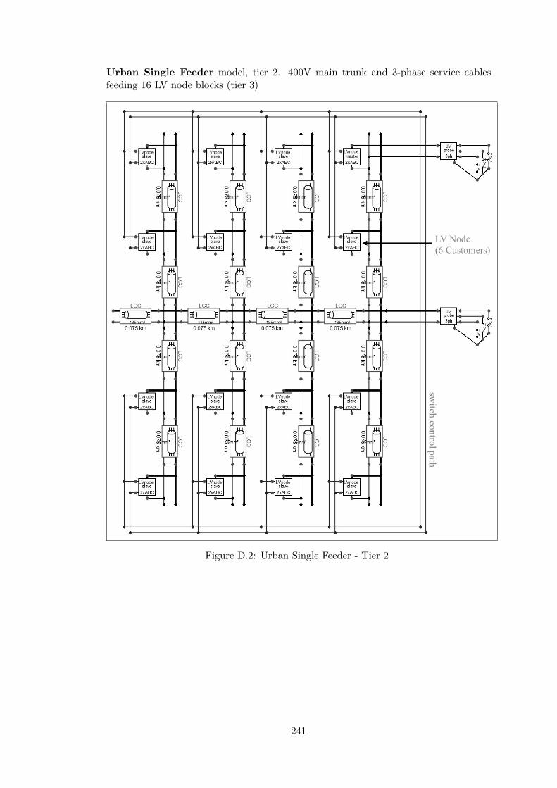
Urban Single Feeder model, tier 2. 400V main trunk and 3-phase service cablesfeeding 16 LV node blocks (tier 3)


241

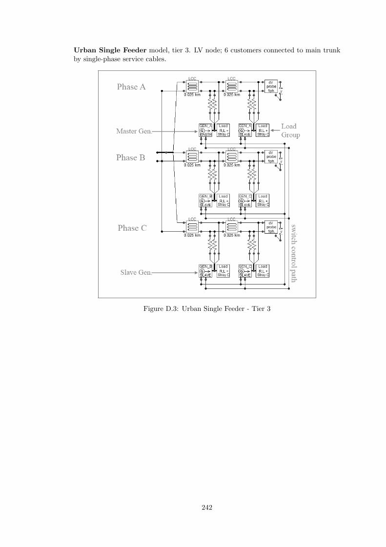
Urban Single Feeder model, tier 3. LV node; 6 customers connected to main trunkby single-phase service cables.


242

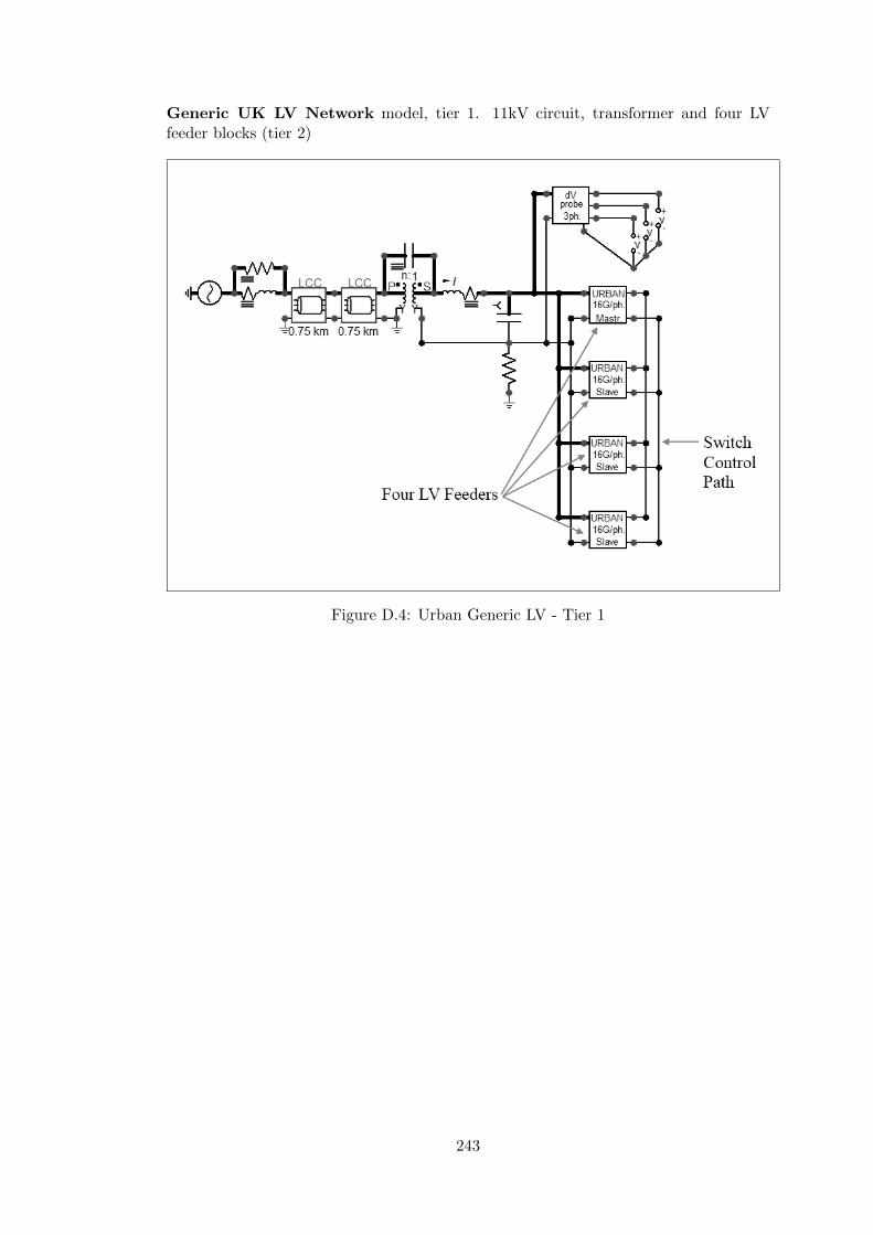
Generic UK LV Network model, tier 1. 11kV circuit, transformer and four LVfeeder blocks (tier 2)

Figure D.4: Urban Generic LV - Tier 1

243

Generic UK LV Network model, tier 2. Identical to the single feeder case (figureD.2)


244

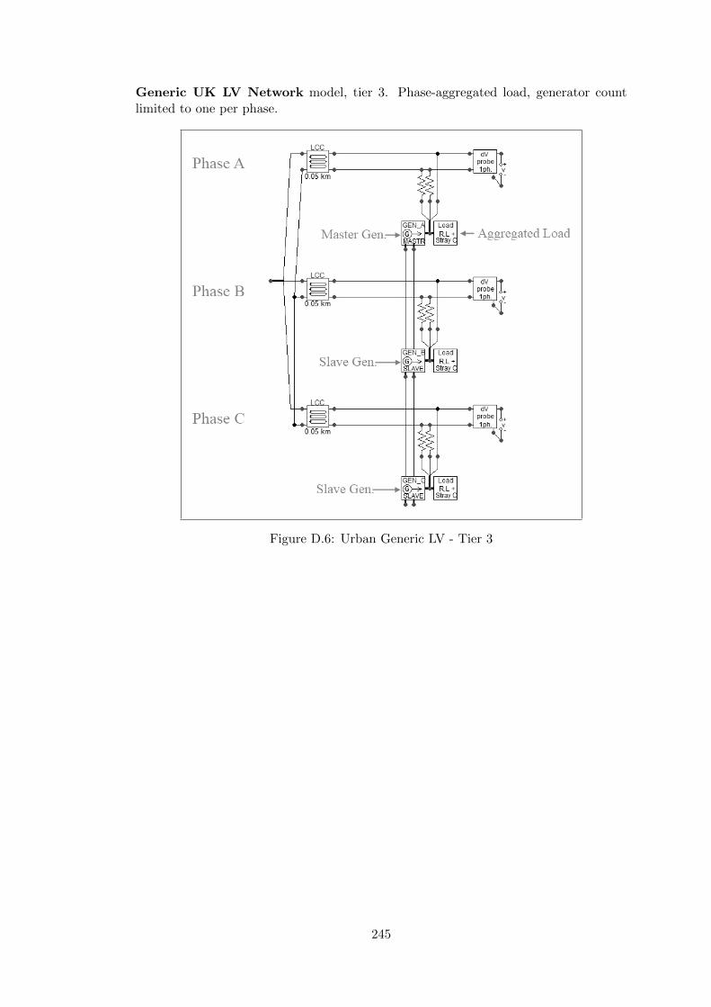
Generic UK LV Network model, tier 3. Phase-aggregated load, generator countlimited to one per phase.


245

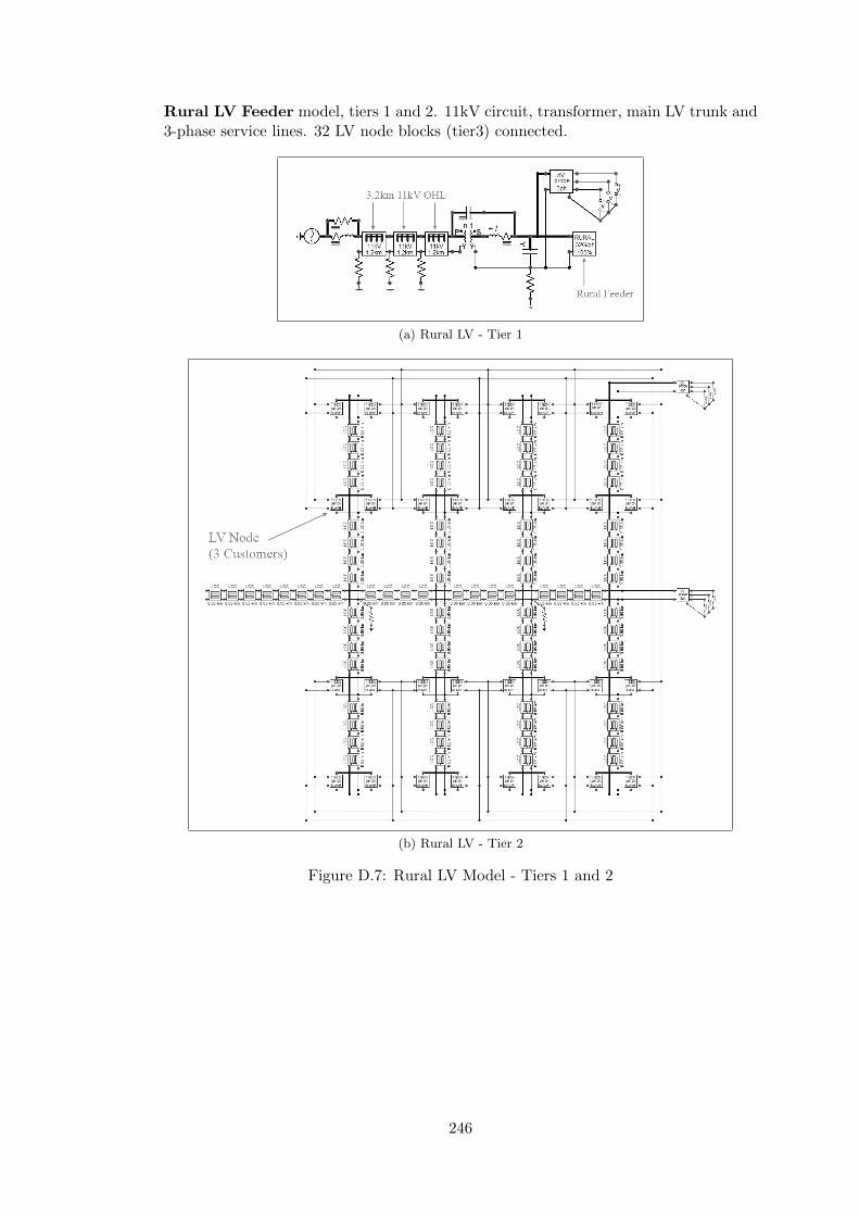
Rural LV Feeder model, tiers 1 and 2. 11kV circuit, transformer, main LV trunk and3-phase service lines. 32 LV node blocks (tier3) connected.

(a) Rural LV - Tier 1

(b) Rural LV - Tier 2

Figure D.7: Rural LV Model - Tiers 1 and 2

246

Rural LV Feeder model, tier 3. One customer per phase, connected by single-phaseoverhead service lines.

Figure D.8: Rural LV - Tier 3

247

∆V Measurement Blocks with notch filter circuitry; Single and Three-phase.

(a) Single-Phase

(b) Three-Phase

Figure D.9: Voltage Measurement Blocks

248

D.2 Statistical Switch Timing

Table D.1: Master Switch (Closing, Phase A)

Mean Time Preceding VA=0 Std.Dev. Distribution

sw1 (master) 0.76ms 92.0µs Gaussian

Table D.2: Slave Switches (Closing, All Phases)

Phase A Phase B Phase C

Delay Std.Dev. Delay Std.Dev. Delay Std.Dev. Distr.

sw1 0ms 92.0µs 6.67ms 92.0µs 13.33ms 92.0µs Gaussian

sw2 98.5µs 33.1µs 6.765ms 33.1µs 13.432ms 33.1µs Gaussian

swi 6.75ms 1.876ms 13.42ms 1.876ms 20.08ms 1.876ms Uniform

Table D.3: Inrush Bypass Switch (Opening, All Phases)

Delay Folowing swi Std.Dev. Distribution

swc 10.0ms 0ms Uniform

249

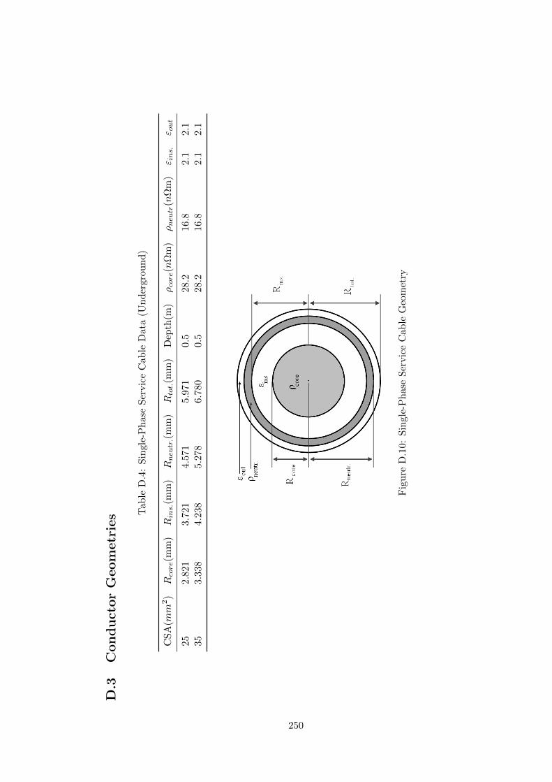
D.3

Con

du

ctor

Geom

etr

ies T

able

D.4

:S

ingl

e-P

has

eSer

vic

eC

able

Dat

a(U

nd

ergr

oun

d)

CSA

(mm

2)

Rcore(m

m)

Rins.

(mm

)Rneutr.(

mm

)Rtot.(m

m)

Dep

th(m

)ρcore(n

Ωm

)ρneutr

(nΩ

m)

ε ins.

ε out

252.

821

3.72

14.

571

5.97

10.

528

.216.8

2.1

2.1

353.

338

4.23

85.

278

6.78

00.

528

.216.8

2.1

2.1

Fig

ure

D.1

0:Sin

gle-

Phas

eS

ervic

eC

able

Geo

met

ry

250

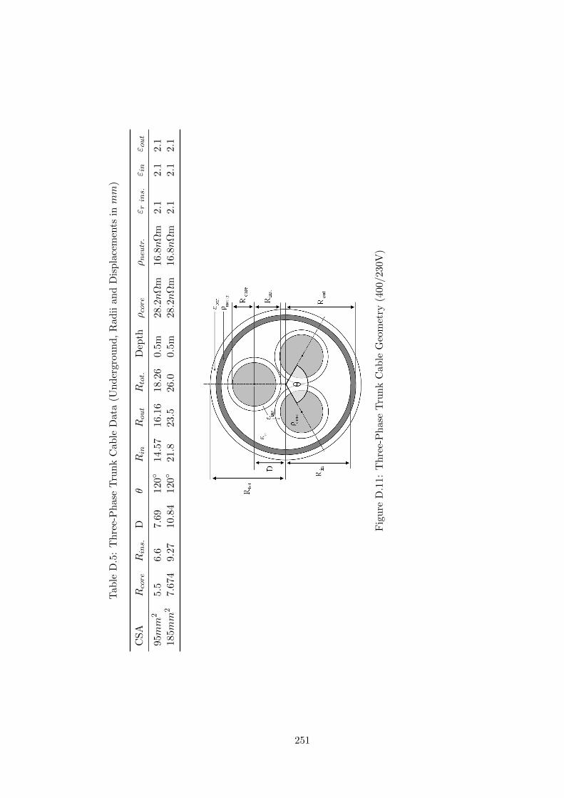
Tab

leD

.5:

Th

ree-

Ph

ase

Tru

nk

Cab

leD

ata

(Und

ergr

oun

d,

Rad

iian

dD

ispla

cem

ents

inmm

)

CSA

Rcore

Rins.

Dθ

Rin

Rout

Rtot.

Dep

thρcore

ρneutr.

ε rins.

ε in

ε out

95mm

25.

56.

67.

6912

0

14.5

716

.16

18.2

60.

5m28

.2n

Ωm

16.8n

Ωm

2.1

2.1

2.1

185mm

27.

674

9.27

10.8

412

0

21.8

23.5

26.0

0.5m

28.2n

Ωm

16.8n

Ωm

2.1

2.1

2.1

Fig

ure

D.1

1:T

hre

e-P

has

eT

runk

Cab

leG

eom

etry

(400

/230

V)

251

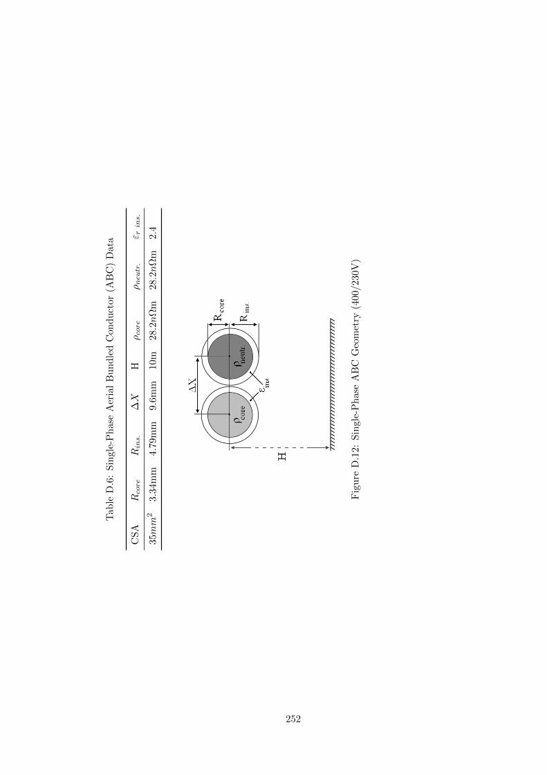
Tab

leD

.6:

Sin

gle-

Ph

ase

Aer

ial

Bun

dle

dC

ond

uct

or(A

BC

)D

ata

CSA

Rcore

Rins.

∆X

Hρcore

ρneutr.

ε rins.

35mm

23.

34m

m4.

79m

m9.

6mm

10m

28.2n

Ωm

28.2n

Ωm

2.4

Fig

ure

D.1

2:S

ingl

e-P

has

eA

BC

Geo

met

ry(4

00/2

30V

)

252

Tab

leD

.7:

Th

ree-

Ph

ase

Aer

ial

Bund

led

Con

duct

or(A

BC

)D

ata

CSA

Rcore

Rins.

∆X

∆Y

Hρcore

ρneutr.

ε rins.

70mm

24.

9mm

6.39

mm

12.8

mm

12.8

mm

10m

28.2n

Ωm

28.2n

Ωm

2.4

120mm

26.

5mm

8.2m

m16

.4m

m16

.4m

m10

m28

.2n

Ωm

28.2n

Ωm

2.4

Fig

ure

D.1

3:T

hre

e-P

has

eA

BC

Geo

met

ry(4

00/2

30V

)

253

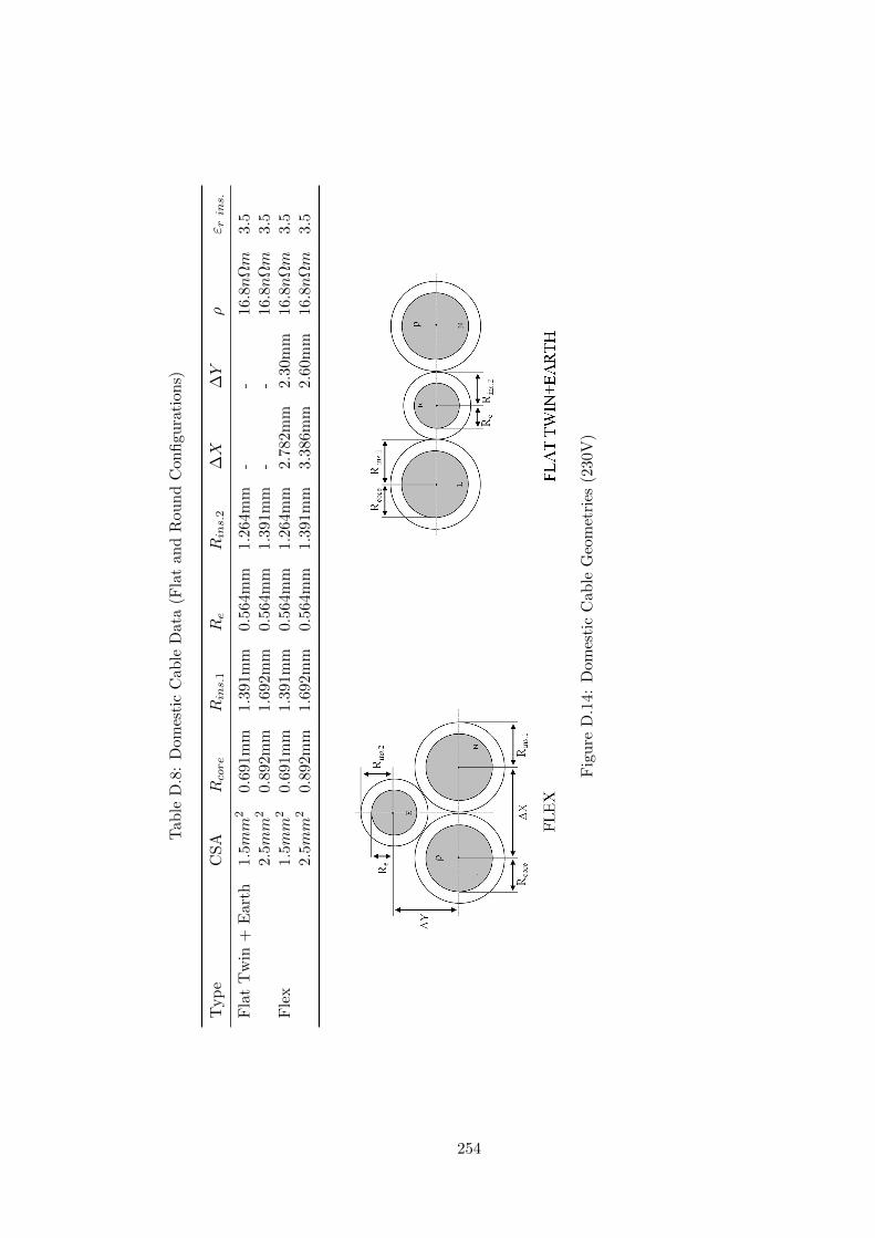
Tab

leD

.8:

Dom

esti

cC

able

Dat

a(F

lat

and

Rou

nd

Con

figu

rati

ons)

Typ

eC

SA

Rcore

Rins.

1Re

Rins.

2∆X

∆Y

ρε r

ins.

Fla

tT

win

+E

arth

1.5mm

20.

691m

m1.

391m

m0.

564m

m1.

264m

m-

-16.8n

Ωm

3.5

2.5mm

20.

892m

m1.

692m

m0.

564m

m1.

391m

m-

-16.8n

Ωm

3.5

Fle

x1.

5mm

20.

691m

m1.

391m

m0.

564m

m1.

264m

m2.

782m

m2.

30m

m16.8n

Ωm

3.5

2.5mm

20.

892m

m1.

692m

m0.

564m

m1.

391m

m3.

386m

m2.

60m

m16.8n

Ωm

3.5

Fig

ure

D.1

4:D

omes

tic

Cab

leG

eom

etri

es(2

30V

)

254

D.4 Cable Propagation Tests (Domestic)

The following plots are the results of low voltage square pulse and step propagationtesting of domestic cables, undertaken in the Cardiff School of Engineering PowerSystems Laboratory. The signal source was a Thandar TG105 pulse generator andmeasurements were made using a LeCroy Waverunner 64Xi oscilloscope. Two cablesamples were subjected to test, with the following configurations:

1. Flat Twin and Earth with solid copper conductors

2. Flex with stranded copper conductors

Each 12m cable section was double PVC insulated with a 2.5mm2 conductor CSA(1.5mm2 Protective Earth), and held at a fixed height of approximately 1m aboveground, as depicted in Figure D.15.

Figure D.15: Test Configuration for Cable Travel Tests

The test configuration has been reconstructed in EMTP using an empirical voltagesource representation of the pulse generator. Results obtained using four variants ofeach cable model (Pi, Bergeron, JMarti and Noda) are plotted for comparison.

255

D.4.1 Open Circuit Test - Square Pulse

Flat Twin and Earth configuration, pulse applied between Live and Neutral.

(a) Sending End

(b) Receiving End (Open)

Figure D.16: Flat Twin and Earth - Measured Live-Neutral

256

Flat Twin and Earth configuration, pulse applied between Live and Earth.

(a) Sending End


Figure D.17: Flat Twin and Earth - Measured Live-Earth

257

Circular Flex configuration, pulse applied between Live and Neutral.

(a) Sending End


Figure D.18: Mains Flex - Measured Live-Neutral

258

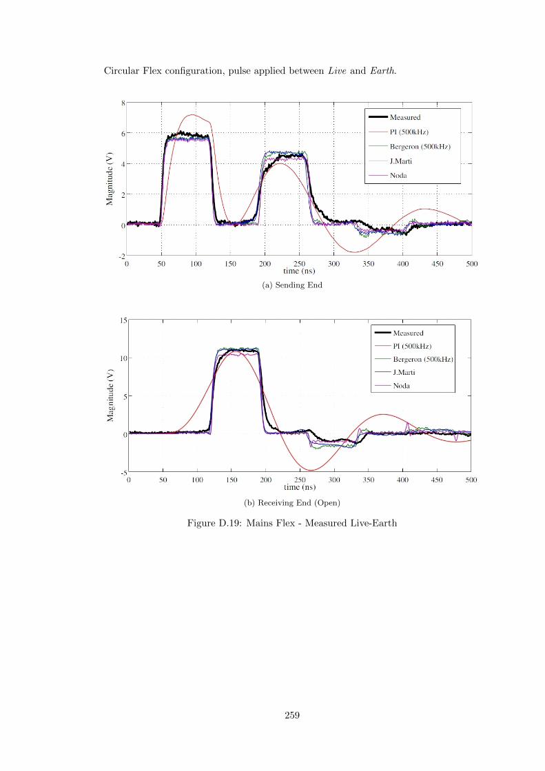
Circular Flex configuration, pulse applied between Live and Earth.

(a) Sending End


Figure D.19: Mains Flex - Measured Live-Earth

259

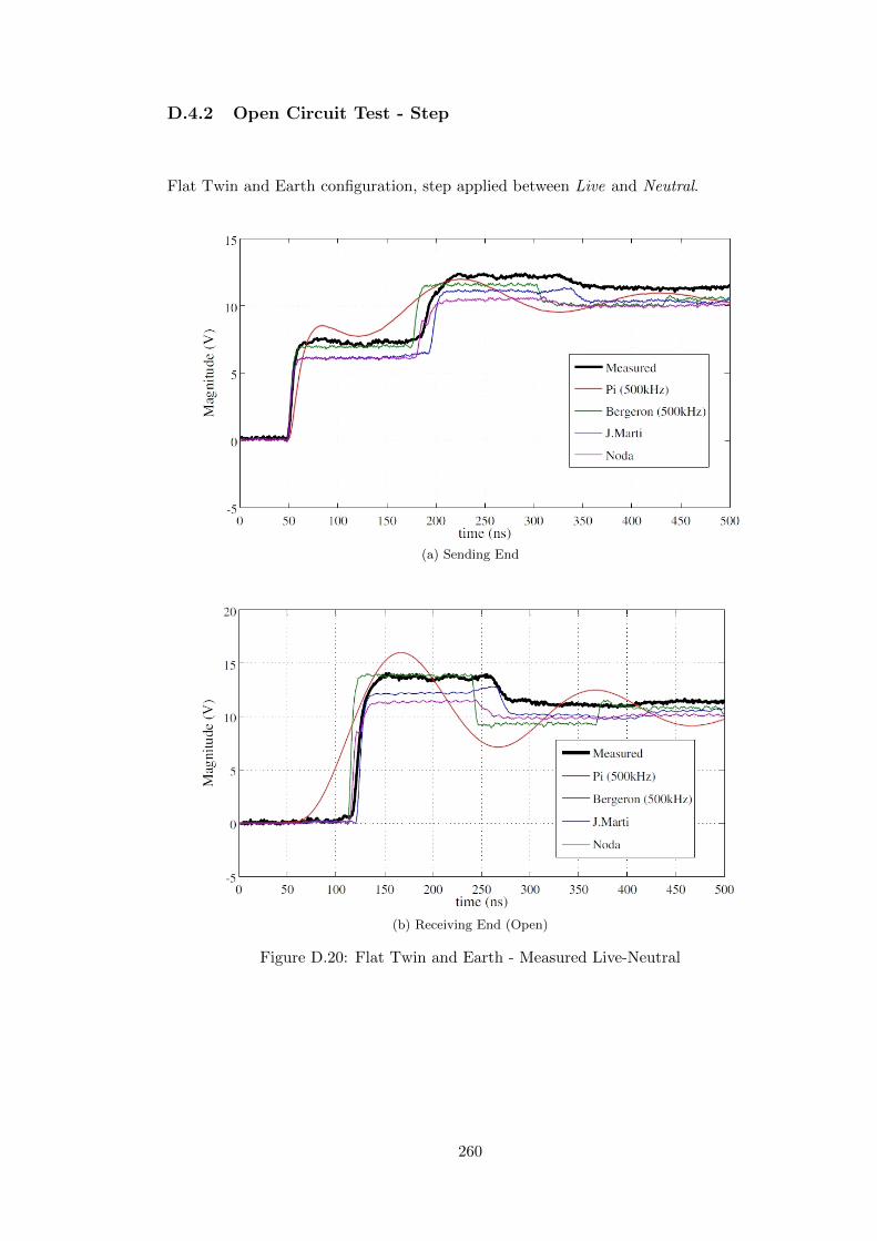
D.4.2 Open Circuit Test - Step

Flat Twin and Earth configuration, step applied between Live and Neutral.

(a) Sending End


Figure D.20: Flat Twin and Earth - Measured Live-Neutral

260

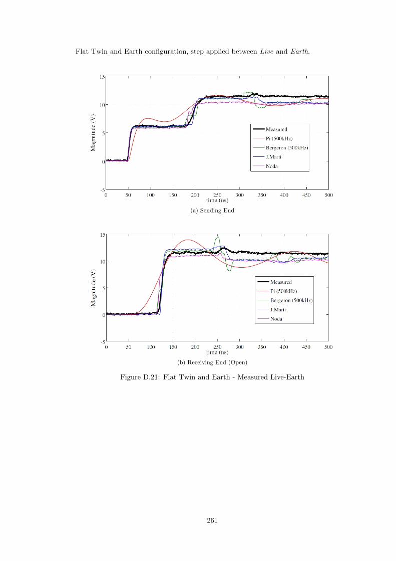
Flat Twin and Earth configuration, step applied between Live and Earth.

(a) Sending End


Figure D.21: Flat Twin and Earth - Measured Live-Earth

261

Circular Flex configuration, step applied between Live and Neutral.

(a) Sending End


Figure D.22: Mains Flex - Measured Live-Neutral

262

Circular Flex configuration, step applied between Live and Earth.

(a) Sending End


Figure D.23: Mains Flex - Measured Live-Earth

263

D.4.3 Short Circuit Test - Square Pulse

Flat Twin and Earth configuration, pulse applied between Live and Neutral.

Figure D.24: Flat Twin and Earth - Pulse Applied Live-Neutral (Receiving End ShortCct)

264

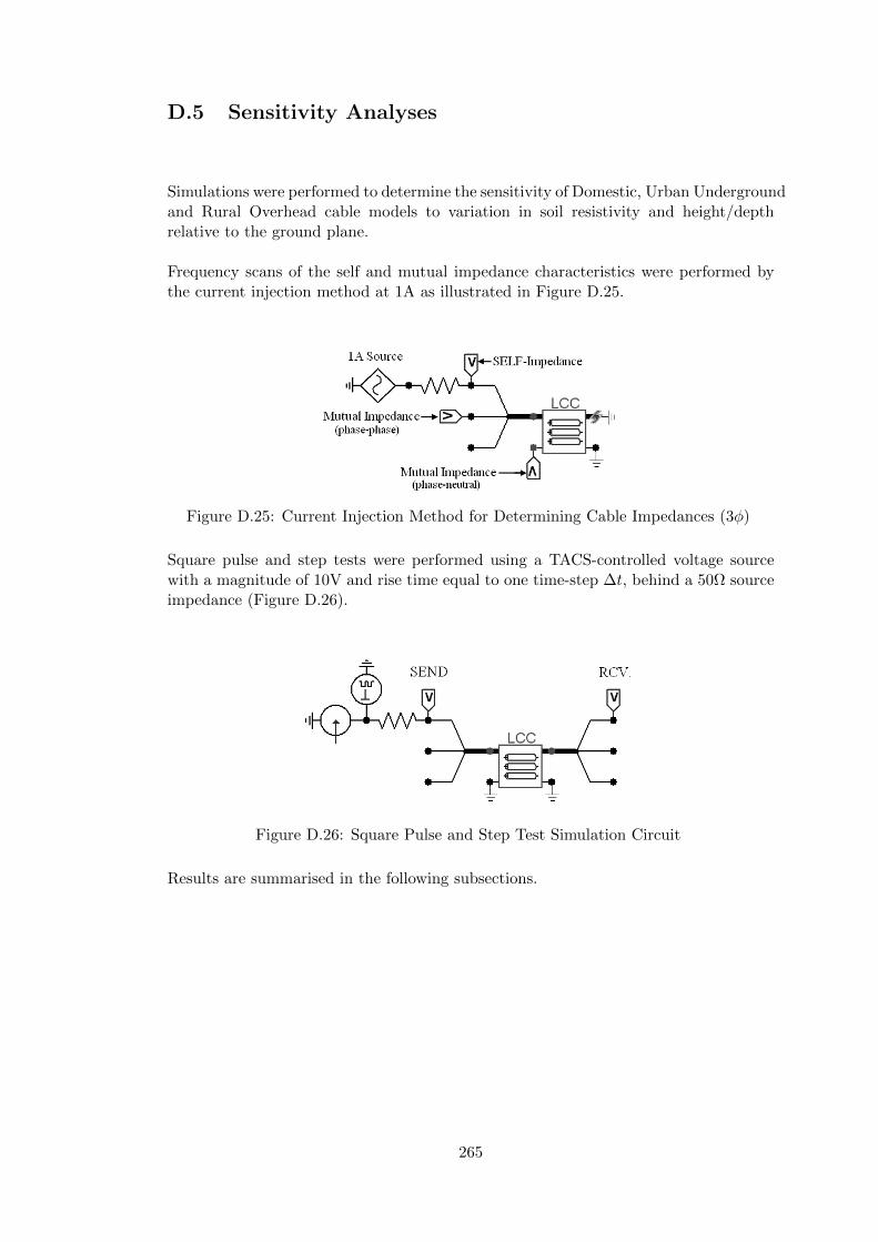
D.5 Sensitivity Analyses

Simulations were performed to determine the sensitivity of Domestic, Urban Undergroundand Rural Overhead cable models to variation in soil resistivity and height/depthrelative to the ground plane.

Frequency scans of the self and mutual impedance characteristics were performed bythe current injection method at 1A as illustrated in Figure D.25.

Figure D.25: Current Injection Method for Determining Cable Impedances (3φ)

Square pulse and step tests were performed using a TACS-controlled voltage sourcewith a magnitude of 10V and rise time equal to one time-step ∆t, behind a 50Ω sourceimpedance (Figure D.26).

Figure D.26: Square Pulse and Step Test Simulation Circuit

Results are summarised in the following subsections.

265

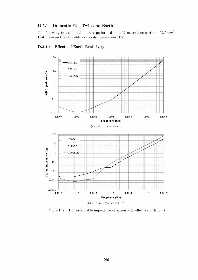
D.5.1 Domestic Flat Twin and Earth

The following test simulations were performed on a 12 metre long section of 2.5mm2

Flat Twin and Earth cable as specified in section D.3.

D.5.1.1 Effects of Earth Resistivity

(a) Self Impedance (L)

(b) Mutual Impedance (L-E)

Figure D.27: Domestic cable impedance variation with effective ρ (h=0m)

266

(a) Square Pulse

(b) Step

Figure D.28: Propagation tests with varying effective ρ (h=0m)

267



Figure D.29: Domestic cable impedance variation with effective ρ (h=0.5m)

268

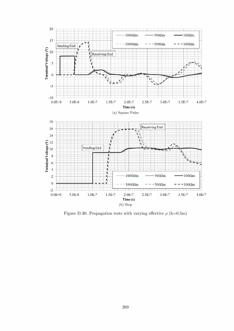
(a) Square Pulse

(b) Step

Figure D.30: Propagation tests with varying effective ρ (h=0.5m)

269

Principal observations:

• No discernible dependence of self-impedance on ground resistivity, regardless ofposition relative to the ground plane.

• Mutual impedance independent of ρ except in cases of very low resistivity wherethe conductor separation is of the same order of magnitude as cable position aboveground (e.g. inside a metallic conduit).

• Minor decrease in phase velocity with increasing ρ.

270

D.5.1.2 Effect of Height Relative to Ground Plane



Figure D.31: Domestic cable impedance variation with height (ρ=500Ωm)

271

(a) Square Pulse

(b) Step

Figure D.32: Propagation tests with varying height (ρ=500Ωm)


• Beyond h=2cm, self and mutual impedances are independent of proximity toground at frequencies in excess of 10kHz.

• For cables at surface (h=0), both self and mutual impedances are significantlyreduced at high frequency.

• Increased cable surge impedance with height (source impedance fixed: 50Ω)

• Increased propagation velocity with height

272

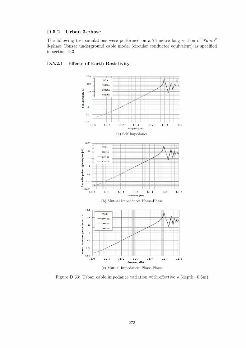
D.5.2 Urban 3-phase

The following test simulations were performed on a 75 metre long section of 95mm2

3-phase Consac underground cable model (circular conductor equivalent) as specifiedin section D.3.


(a) Self Impedance

(b) Mutual Impedance: Phase-Phase

(c) Mutual Impedance: Phase-Phase

Figure D.33: Urban cable impedance variation with effective ρ (depth=0.5m)

273

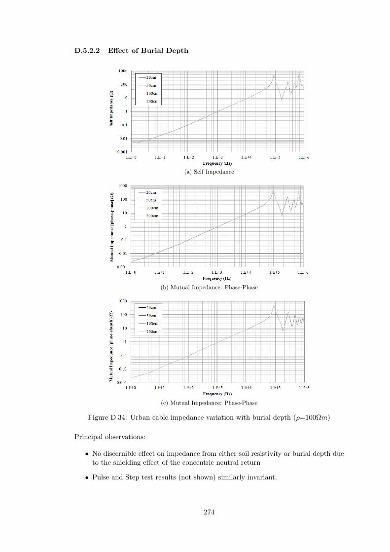
D.5.2.2 Effect of Burial Depth

(a) Self Impedance


(c) Mutual Impedance: Phase-Phase

Figure D.34: Urban cable impedance variation with burial depth (ρ=100Ωm)


• No discernible effect on impedance from either soil resistivity or burial depth dueto the shielding effect of the concentric neutral return

• Pulse and Step test results (not shown) similarly invariant.

274

D.5.3 Rural 3-phase ABC

The following test simulations were performed on a 50 metre long section of 70mm2

3-phase Aerial Bundled Conductor model as specified in section D.3.


(a) Self Impedance


Figure D.35: ABC cable impedance variation with soil resistivity (height=10m)

275

(a) Square Pulse

(b) Step

Figure D.36: Propagation tests (ABC) with varying soil resistivity (h=10m)

276

D.5.3.2 Effect of Pole Height

(a) Self Impedance


Figure D.37: ABC cable impedance variation with pole height (ρ = 100Ωm)

277

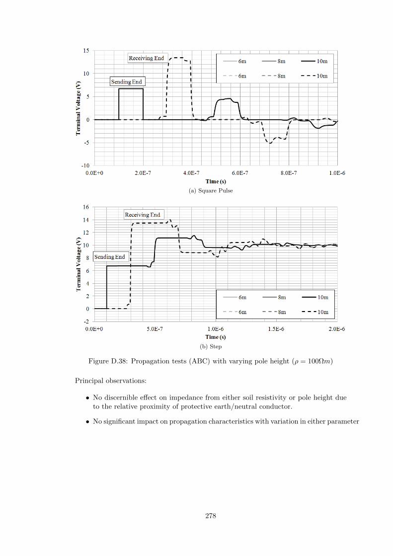
(a) Square Pulse

(b) Step

Figure D.38: Propagation tests (ABC) with varying pole height (ρ = 100Ωm)


• No discernible effect on impedance from either soil resistivity or pole height dueto the relative proximity of protective earth/neutral conductor.

• No significant impact on propagation characteristics with variation in either parameter

278

D.6 Cable CSA Equivalence

In the absence of an established finite-element modelling preprocessor to the LCCroutine in EMTP-ATP, a number of electrostatic simulations were performed in order todevelop circular-conductor equivalents of sectored cables common to Urban undergroundnetworks. In making the transition between geometries, conductor cross-sectional areasare preserved but the use of circular conductors increases the overall cable diameter, andmore significantly it reduces both inter-phase and phase-neutral capacitances (Cp,Cn)as depicted in Figure D.39.

Figure D.39: Inter-phase and phase-neutral capacitances of Sectored and Circular cablemodels

This may be rectified by the introduction of a fictitious permittivity εr’ for theinsulation of the circular cable model which, assuming an homogeneous dielectric regionhas no impact on the series impedance of the cable. As shunt conductance is ignoredin the model, there is no need to scale to account for dielectric loss. CapacitancesCp and Cn were determined by finite element analysis using the Electromagnetic Fieldpackage SLIM. Figure D.40 depicts the simulated sectored cross-section and its fieldand equipotential distributions in even and odd mode excitation.

279

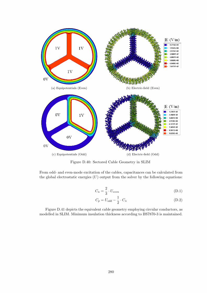
(a) Equipotentials (Even) (b) Electric-field (Even)

(c) Equipotentials (Odd) (d) Electric-field (Odd)

Figure D.40: Sectored Cable Geometry in SLIM

From odd- and even-mode excitation of the cables, capacitances can be calculated fromthe global electrostatic energies (U) output from the solver by the following equations:

Cn =2

3· Ueven (D.1)

Cp = Uodd −1

2· Cn (D.2)

Figure D.41 depicts the equivalent cable geometry employing circular conductors, asmodelled in SLIM. Minimum insulation thickness according to BS7870-3 is maintained.

280

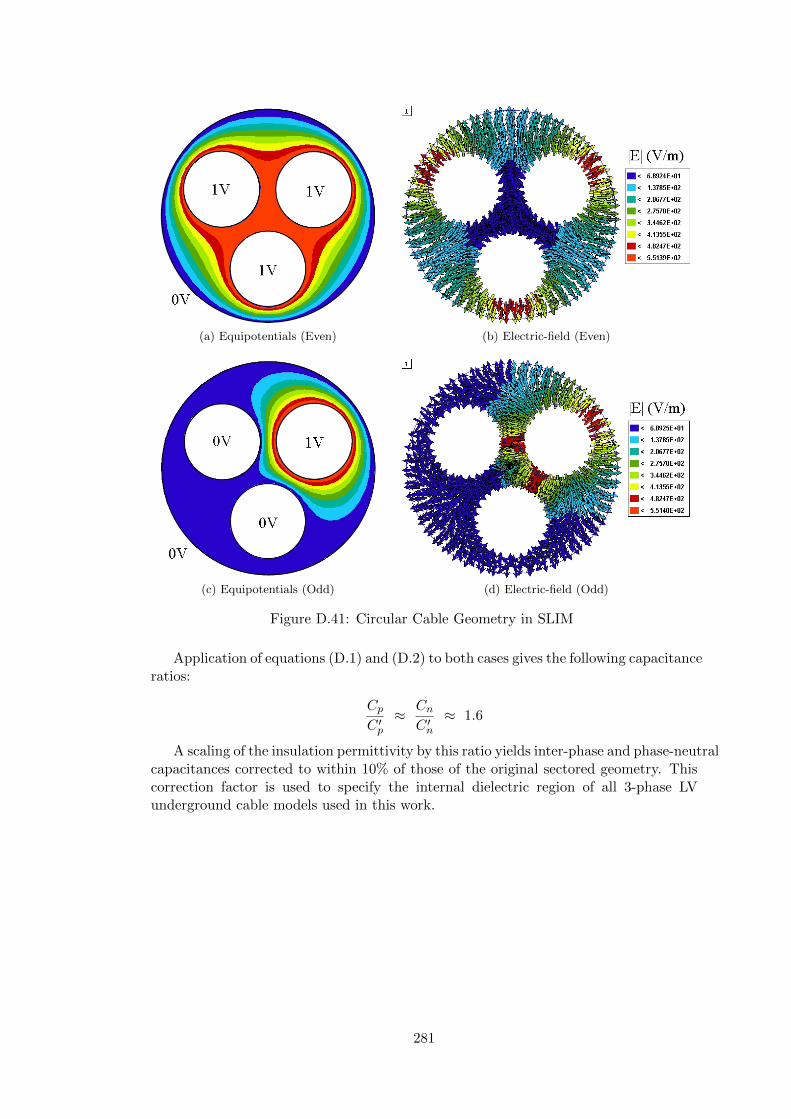
(a) Equipotentials (Even) (b) Electric-field (Even)

(c) Equipotentials (Odd) (d) Electric-field (Odd)

Figure D.41: Circular Cable Geometry in SLIM

Application of equations (D.1) and (D.2) to both cases gives the following capacitanceratios:

CpC ′p≈ Cn

C ′n≈ 1.6

A scaling of the insulation permittivity by this ratio yields inter-phase and phase-neutralcapacitances corrected to within 10% of those of the original sectored geometry. Thiscorrection factor is used to specify the internal dielectric region of all 3-phase LVunderground cable models used in this work.

281

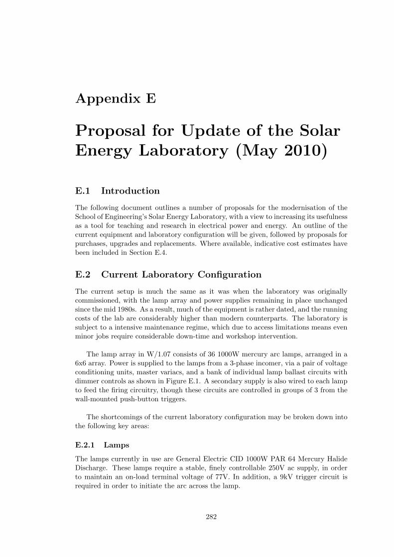
Appendix E

Proposal for Update of the SolarEnergy Laboratory (May 2010)

E.1 Introduction

The following document outlines a number of proposals for the modernisation of theSchool of Engineering’s Solar Energy Laboratory, with a view to increasing its usefulnessas a tool for teaching and research in electrical power and energy. An outline of thecurrent equipment and laboratory configuration will be given, followed by proposals forpurchases, upgrades and replacements. Where available, indicative cost estimates havebeen included in Section E.4.

E.2 Current Laboratory Configuration

The current setup is much the same as it was when the laboratory was originallycommissioned, with the lamp array and power supplies remaining in place unchangedsince the mid 1980s. As a result, much of the equipment is rather dated, and the runningcosts of the lab are considerably higher than modern counterparts. The laboratory issubject to a intensive maintenance regime, which due to access limitations means evenminor jobs require considerable down-time and workshop intervention.

The lamp array in W/1.07 consists of 36 1000W mercury arc lamps, arranged in a6x6 array. Power is supplied to the lamps from a 3-phase incomer, via a pair of voltageconditioning units, master variacs, and a bank of individual lamp ballast circuits withdimmer controls as shown in Figure E.1. A secondary supply is also wired to each lampto feed the firing circuitry, though these circuits are controlled in groups of 3 from thewall-mounted push-button triggers.

The shortcomings of the current laboratory configuration may be broken down intothe following key areas:

E.2.1 Lamps

The lamps currently in use are General Electric CID 1000W PAR 64 Mercury HalideDischarge. These lamps require a stable, finely controllable 250V ac supply, in orderto maintain an on-load terminal voltage of 77V. In addition, a 9kV trigger circuit isrequired in order to initiate the arc across the lamp.

282

Figure E.1: Basic Lamp Supply Circuitry

Since harmonisation of the university supply to the European 230V standard, thelamps in the array have been running at below their rated voltage, a problem exacerbatedby a number of faulty power factor correction capacitors. Discharge lamps of this typeare by their nature highly sensitive to variations in voltage, and will typically notignite if the supply drops below approximately 90% of the rated value. A small rangeof dimming may be achieved by varying the supply between 90-100% of the rated value,however the functionality of the control variacs has largely been lost since moving to230V, such that at full supply the lamps are confined to the lower end of their operatingrange.

The reduced and varied terminal voltages mean that typical lamp brightness isconsiderably lower than in the original specification, lamp operating lifetimes are reduced,and certain lamps will often refuse to fire on the first attempt, requiring a 30-minuteheat/cool cycle for those lamps which operate successfully before re-firing. At a replacementcost in eccess of £150 per lamp, the present system is economically unsustainable.

E.2.2 Ignition

Ignition for the lamps is provided by 12 normally-open 3-phase switches mounted onthe wall of the laboratory. When a switch is held closed, power is supplied to the 9kVignition circuits of three of the lamps. The ignition switches should only remain closedfor maximum of 5 seconds, by which time all three lamps should ignite. As mentionedabove however, ignition is not always successful and one of the lamps will require firingagain.

This is the key problem with the current ignition scheme, in that individual controlof the lamp igniters cannot be achieved if the lamps fire in groups of 3. It is also badpractice to re-fire lamps which are already lit, since this drastically reduces the life ofboth the lamp and igniter. A failed ignition therefore requires that the two operationallamps be cycled through a 10-minute warm-up period, and following extinguishing beallowed to cool for a further 20 minutes to allow the mercury vapor to deposit in thewell of the lamp. Only then can the three lamps be successfully fired again. This makesfailed ignition a major time-consuming factor in any testing regime.

E.2.3 Ballast and PFC

As with all forms of discharge lamp, the solar array requires a ballast in order tomaintain a steady arc across the lamps. In addition, due to the low power factor of

283

such arcs, considerable correction is required in the form of large capacitors across thelamp terminals. Each lamp supply circuit is provided with a large ballast inductor and175uF capacitor in order to maintain near unity power-factor, though this is somewhatcompromised by running at a lower than specified supply voltage.

The ballast and PFC circuitry, although still functional, is no longer suitable for thejob it is required to perform. A number of the ballast units require replacing as theyproduce excessive levels of noise when operational, and some of the PFC capacitorshave failed resulting in drastically reduced lamp terminal voltage.

E.2.4 Dimming

In addition to the lamp ballast, a degree of dimming control was incorporated into theoriginal design through the use of individual supply variacs. The 36 control variacs,mounted on the ballast panels running along the side of the laboratory, allow the supplyvolts to be dropped to approximately 90% of the rated value in order to reduce the arcintensity of individual lamps.

While the benefit of such a scheme in maximising the uniformity of emmittedradiation can easily be appreciated, the functionality has largely been lost since supplyvoltages were reduced to harmonised levels. Running at an upper voltage of 230V nowmeans that lamps are confined to the lower end of their useful range, and any attemptto further reduce the supply volts will quench the arc. Any future scheme based ondischarge lamps and requiring intensity control will need this issue addressing.

In addition to the operational limitations of the dimming circuitry, there is thepractical issue of access and maintanance. Due to the physical size of the control panel,it is not actually possible to bring the lamp array down to ground level for maintenanceas the crane is obstructed. It must therefore be suspended on 1m supports, making itvery difficult to get access to the centre of the array to replace lamps and check thefiring circuits.

E.2.5 General Circuitry and Labelling

Fault-finding and maintenance on the control and ballast circuitry is complicated bya general lack of color-coding and labelling. Faulty circuits need to be traced throughby hand in order to know which ballast, dimmer control or PFC cap relates to whichlamp, and half of the dimmer variacs are unlabelled. This makes it a complex andtime-consuming process to determine the cause of faults on the system.

Since any change in lamp technology will require an overhaul of the supply, afully-labelled, traceable system should be a priority in order to improve accessabilityand cut maintenance down-time.

E.3 Proposals

The following section outlines a number of proposals for upgrading or modernising thelaboratory.

284

E.3.1 Lamp Array and Control Gear

Due to the range of lighting options available, there is no single ideal configuration thata new array should take. Each technology has its benefits and limitations, and the finaldecision will need to strike the best balance between functionality, flexibility and cost.There follows some examples of new configurations, with a breakdown of requirementsin each case.

E.3.1.1 Option 1: Cold-Restrike Mercury Halide Discharge

The first option is to continue with cold-restrike mercury arc lamps, identical to thoseused in the present rig. This would allow continued use of the existing lamp housings,but the power supply, dimming and firing circuitry would require major overhaul.Firstly, the power supply to each lamp would need to be boosted back above 240Vin order to bring the lamps back into a respectable operating range, though as alreadymentioned the dimmable range of the current lamps is small. The easiest way to achievea correct operating voltage would be to adjust upper voltage limit of the master variacs,which should be simple enough as the units are rated for 470V 3 phase.

In addition, ageing PFC and ballast units would need servicing or replacing inorder to balance out performance across the array, and the trigger circuits shouldalso be replaced with modern high-voltage igniters, with individual firing control. Inits current state, due to the limited functionality of the lamp dimming circuitry, theindividual control variacs are of little or no use in any test regime. If dimming capabilitywere deemed a requirement then the supply variacs would need to be maintained,however halogen lamps would be a far more suitable choice in this case due to theirwide operating range.

Figure E.2 depicts the recommended GE setup for cold-restrike lamps. The drawbackof this option, in addition to high replacement cost of faulty equipment and the needto maintain the bulky ballast and PFC banks, is the high lamp replacement cost. Atapproximately £125 + VAT each a full array replacement would cost approximately£5500, with a rated lifetime of 1500 hours. Through the use of individual ignitionswitches, much of the problem caused by the need to cycle lamps between firings isremoved, but it does not negate the need to cycle array between tests. This drawbackcan be overcome by the use of hot-restrike lamps, as outlined in option 2. For a fullcost breakdown of this option, see Section E.4.1.1.

E.3.1.2 Option 2: Hot-Restrike Mercury Halide Discharge

An alternative configuration using hot-restrike discharge lamps could also be implemented.This would eliminate the need to cycle the lamps after each operation, which wouldreduce testing time and also make the lab more suitable for short teaching demonstrations.As with option 1, this would allow us to keep the existing frame and lamp holders, andthe requirements for ballast, PFC and firing switch replacement would be the same.

The main difference in this case would be the need for hot-restrike igniters. Theseare more expensive than their cold-restrike counterparts, with the recommended GEmodel costing about £450 each. Furnishing a complete lab with 36 hot-restrike ignitersrepresents a major expense, and therefore makes this the most expensive option in termsof initial investment. In addition, running costs wuold remain high as hot-restrike lamps

285

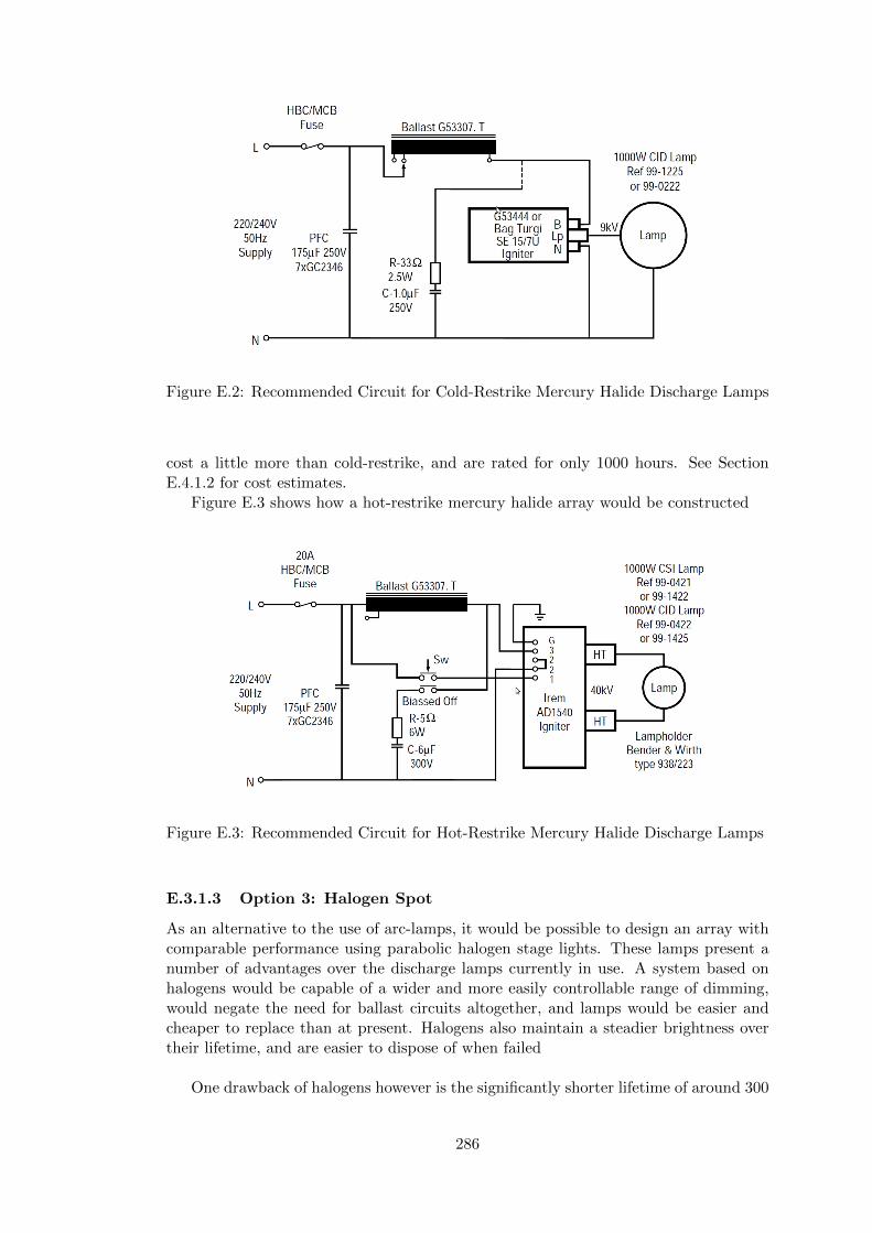
Figure E.2: Recommended Circuit for Cold-Restrike Mercury Halide Discharge Lamps

cost a little more than cold-restrike, and are rated for only 1000 hours. See SectionE.4.1.2 for cost estimates.

Figure E.3 shows how a hot-restrike mercury halide array would be constructed

Figure E.3: Recommended Circuit for Hot-Restrike Mercury Halide Discharge Lamps

E.3.1.3 Option 3: Halogen Spot

As an alternative to the use of arc-lamps, it would be possible to design an array withcomparable performance using parabolic halogen stage lights. These lamps present anumber of advantages over the discharge lamps currently in use. A system based onhalogens would be capable of a wider and more easily controllable range of dimming,would negate the need for ballast circuits altogether, and lamps would be easier andcheaper to replace than at present. Halogens also maintain a steadier brightness overtheir lifetime, and are easier to dispose of when failed

One drawback of halogens however is the significantly shorter lifetime of around 300

286

hours. Lamps will therefore need replacing about four times as often as at present, butat a cost of £20 + VAT per lamp, this still represents a much lower running cost thanat present. There will also be the likely initial investment for 36 new lamp housings,as it is impossible to find PAR 64 halogens with G38 connectors. It may however bepossible to retorofit the existing equipment with adapters, assuming that the currenthousings are capable of dissipating the eccess heat generated by halogen lamps

The most interesting opportunity presented by moving to halogen however is theoption of using an off-the-shelf, robust stage lighting system. This would replace theexisting bulky ballast, PFC and dimming circuitry, which could then be removedentirely, creating useful additional space for storage and maintenance. In its placewould be a compact, wall-mounted 36-channel power-electronic dimmer, with a DMXconnection to desk-mounted control board which could be located either in the laboratoryitself, or in the 2nd floor control room.

This would allow the user to start up, dim, and shut down each lamp individuallyfrom a workstation, giving a degree of flexibility and control not possible with thecurrent setup. A DMX controller could also be programmed to simulate the changein light intensity throughout the day if required. Such a system could be purchasedfor less than £2500, making this a more attractive initial investment than moving tohot-restrike discharge lamps. Figure E.4 provides an example of the equipment requiredto implement such a system. For cost estimates, see Section E.4.1.3.

(a) Halogen PAR (b) 18-Channel Dimmer Unit (c) DMX Control Panel

Figure E.4: Stage-Lighting System Components

E.3.1.4 Option 4: Halogen Flood

An alternative to spot lamps is to use halogen flood lights. The hardware requirementsin this case would be identical to that outlined in option 3, as lamp ratings andconnections would be the same. This highlights another degree of flexibility affordedby a halogen-based system in that it is possible to switch relatively quickly and cheaplybetween different lamps as the present test regime requires.

While spot lamps are useful for high intensity or small-area testing, a flood arraywould be ideal for maintaining a high degree of uniformity over large areas such asa militple-panel photovoltaic array. This capability would greatly reduce the effect oflocalised hot-spots which currently limits the test performance of PV cells. Halogen

287

floods have the same unit cost and rated lifetime as spots, with a full compliment of 36costing less than £1000.

E.3.2 Access and Maintenance

A key contributor to laboratory downtime is the lack of dedicated equipment for thepurpose of lamp replacement and general maintenance. At present, if a lamp is lost fromthe array the one-tonne rig must be transferred to a crane hoist, moved horizontally intoposition and lowered face-down onto four support structures at a height of about 1mfrom the ground. Since this arrangement only allows access to the lamps along the edgesof the array, any central lamps must be replaced with the array in an upright postionwhere they can be reached from the floor. This allows the rig to swing dangerously onthe crane hoist during maintenance which should be avoided.

To address these problems, the workshop recommendation is to purchase a dedicatedlightweight scaffold tower of a suitable height to reach each of the 36 lamps in its uprightposition. Towers such as those shown in Figure E.5 are available for about £700, witha working height of 5.5m, or £1000 for working height of 7.15m.

(a) 3.5m Platform (b) 5.5m Platform

Figure E.5: Lightweight Mobile Scaffold Towers

Mr. Paul Farrugia has expressed concern, particularly from a safety perspective,over the continued use of the crane hoist for lifting and moving the lamp array. It issuggested that the current system be replaced with an X-Y drive system running eitheron a pair of fixed uprights or a rolling floor-mounted rig. This would give us the sameif not a greater degree of manoeuvreability, allowing us to bring the array as close asrequired to the test object, wile completely eliminating the problem of the rig swingingand bouncing on the crane. Options for implementation will need to be discussed ingreater detail with the mechanical workshop.

If the crane system can not be replaced, then to overcome the problem of the uprightrig swinging during maintenance work, it is recommended that covered anchor pointsbe sunk into the floor of the laboratory, allowing use of heavy-duty ratchet straps to tiethe rig in place. This should be combined with a load-bearing cushion to protect the

288

rig and floor surface from impact with the ground. It is recommended that the craneunits be fitted with variable speed drives in order to soften the lift/drop process, whichat present causes the rig to jerk violently whenever the clutch is engaged. The presentbehaviour makes it difficult to lower the rig to the floor without rebounding, and alsoplaces excessive stress on the structure. The horizontal crane drives would also benefitfrom some additional control due to a slight speed imbalance between the right andleft units. Over time this causes the rig to shift off-center, a problem which could berectified either by matching the speeds or by providing a degree of individual control toeach crane. Speed selectors and directional controls could be combined with the lampcontrol panel to provide a single control unit

In addition to crane lift control drives, the oscillation of the rig could also be reducedby fitting dampers between the inner and outer frames of the array. This would reducethe mechanical stress on the wiring, lamp housings and tilt control drives when thearray is being manoeuvred into position.

Another important aspect to address is the tilt mecanism of the array. This iscurrently provided by a low-speed motor on a chain drive attatched to the tilt axis ofthe array. The problem here is due to the inertia of the rig, which when the tilt driveis activated causes its movement to lag the motor. The rotation is initially taken up bythe chain, and the rig will then swing precariously into place to balance out. This is adifficult problem to address as the array is required to sit on the chain support whenbeing manoeuvred, however a finer control of the motor position would be beneficialand help to reduce this effect.

E.3.3 Working Environment

Any laboratory test based on characterisation of devices or the collection of some formof statistical data requires the user to spend significant amounts of time working inthe laboratory. The working environment should therefore be comfortable, and provideample space for test equipment, tools and components.

The lab should be provided with desk space and chairs for at least two peopleto work for extended periods, and ideally a work table with clamps for building testequipment, soldering etc. Storage is currently provided by three metal cabinets anda cupboard/drawer unit at the back of the lab which is likely sufficient for currentneeds, but both need sorting, emptying and labelling in order to become useful. Thelaboratory also requires suitable regular and recycling waste disposal bins

It would also be beneficial to reinstate the 2nd floor control room, which wouldbe used as a workspace and also to house any new control gear such as DMX dimmerboards. This woulg greatly reduce the time spent working under the lights, particularlyfor lengh characterisation or data-acquisition tests. It is also recommended that screeningfilm be applied to the 2nd floor corridor windows to minimise distraction and avoiddazzling passers-by

Some thought will need to be given to heating of the laboratory, as winter temperaturesindoors drop to around 10 C without the lamps in operation, making it almostimpossible to work. This is mostly due to poor insulation around the bay doors,but is also partly attributable to poor draught exclusion between W/1.07 and 1.08.The separator between the two labs currently consists of a vertical shutter door, with

289

the doorway blocked up with three large slabs of polystyrene foam. This does littleto block draughts from next door, and the foam blocks consequentially move aboutwhich is noisy and distracting. It is recommended that the door be replaced with amore suitable alternative which provides a comparable degree of insulation between therooms, while allowing access when necessary.

With regard to equipment specific to power-based measurememnt and testing, thereare a number of tools which would be useful to have as permanent fixtures in the lab,such as a good quality oscilloscope, power analyser, a set of DC/high frequency voltageand current probes, and a range of high voltage leads, connectors, probes and commonlyused components for quicky making up custom test equipment. More sophisticatedequipment would need to be obtained on a project-specific basis.

One important addition from an electrical perspective however would be the provisionof solid earthing points around the lab. These are currently not provided for, and theonly option for earthing is to return to the supply earth which is unsuitable for anyform of high voltage testing. Electrical connections to the laboratory metalwork ora dedicated earthing rod should be made available, together with a ready supply ofearth-braid for the connection of individual pieces of equipment.

E.3.4 Health and Safety

On the subject of health and safety, there are a number of recommendations forimprovement. First and foremost should be the provision of suitable safety eyewearfor working under high-intensity lights. Though the risk of dangerous levels of UVexposure are minimal, the visible light intensity is high enough to cause serious eyedamage. Filtered safety spectacles can be purchased cheaply and should be providedfor all work in the laboratory, and also to visitors whenever the array is operational. It isalso recommended that dedicated safety headwear and gloves be provided for wheneverthe array is brought down on the crane and lamps replaced.

Regarding the safety concerns of manoeuvring the solar array, the majority ofconcerns are summarised in Section E.3.2, and need not be repeated here. The additionof a lightweight scaffold tower will however require that correct training be undertakenfor working at height, and suitable electrical safety provisions and guidelines will needto be available if the lab is to be used for ongoing work on photovoltaics.

290

E.4

Cost

Esi

mate

s

The

follw

oin

gse

ctio

nsu

mm

aris

esth

em

ater

ial

cost

wh

ere

pos

sible

ofth

epro

pos

als

inse

ctio

nE

.3.

Th

em

ajo

rity

of

qu

ote

sare

still

pen

din

gas

of

11/0

5/20

10

E.4

.1L

am

pA

rray

and

Contr

ol

Gear

E.4

.1.1

Opti

on

1:

Cold

-rest

rike

Dis

charg

eL

am

ps

(main

tain

ing

curr

ent

setu

p)

Tab

leE

.1:

Init

ial

Cos

ts

Item

Unit

Cost

(£)

Qty

Su

bto

tal

(£)

VA

T(£

)T

ota

l(£

)Su

pp

lier

Lam

ps:

GE

CID

1000

W99

-122

5G

38126.0

036

4536.0

0793.8

05329.8

0A

Clighti

ng

uk

Ignit

ors:

G53

444

TH

OR

N10

00W

SE

15/7

W40.0

036

1440.0

0252.0

01692.0

0sl

bb

reaker

slt

dR

epla

cem

ent

Bal

last

s-

10

--

-U

nknow

nR

epla

cem

ent

PF

C-

10

--

-U

nknow

n

10A

Sin

gle

Ph

ase

Mom

enta

ryT

rigg

erS

wit

ches

10.6

336

22.6

83.9

726.6

5R

S

Tab

leE

.2:

Ongo

ing

Cos

ts

Item

Unit

Cost

(£)

Qty

Su

bto

tal

(£)

VA

T(£

)T

ota

l(£

)Su

pp

lier

Lam

ps:

GE

CID

1000

W99

-122

5G

38126.0

036

4536.0

0793.8

05329.8

02

AC

lighti

ng

uk

1E

xis

ting

trig

ger

panel

sca

nb

ere

-use

d2C

om

ple

tela

mp

repla

cem

ent

ever

y1200-1

500

lam

p-h

ours

291

E.4

.1.2

Opti

on

2:

Hot-

rest

rike

Dis

charg

eL

am

ps

Tab

leE

.3:

Init

ial

Cos

ts

Item

Unit

Cost

(£)

Qty

Su

bto

tal

(£)

VA

T(£

)T

ota

l(£

)Su

pp

lier

Lam

ps:

GE

CID

1000

W99

-142

5G

38H

R128.5

036

4626.0

0809.5

55435.5

5A

Clighti

ng

uk

Ignit

ors:

IRE

MA

D15

40ig

nit

er400

36

14,4

00.0

02520.0

016920.0

0un

know

nR

epla

cem

ent

Bal

last

s-

10

--

-U

nknow

nR

epla

cem

ent

PF

C-

10

--

-U

nknow

n

10A

Sin

gle

Ph

ase

Mom

enta

ryT

rigg

erS

wit

ches

10.6

336

22.6

83.9

726.6

5R

S10

ASin

gle

Ph

ase

Lat

chin

gT

rigg

erSw

itch

es0.8

536

30.6

05.3

635.9

6R

SA

dd

itio

nal

bia

sR

Cnet

wor

k-

--

--

Tab

leE

.4:

Ongo

ing

Cos

ts

Item

Unit

Cost

(£)

Qty

Su

bto

tal

(£)

VA

T(£

)T

ota

l(£

)Su

pp

lier

Lam

ps:

GE

CID

1000

W99

-142

5G

38H

R128.5

036

4626.0

0809.5

55435.5

52

AC

lighti

ng

uk

1E

xis

ting

trig

ger

panel

sca

nb

ere

-use

d2C

om

ple

tela

mp

repla

cem

ent

ever

y1200-1

500

lam

p-h

ours

292

E.4

.1.3

Opti

ons

3/4:

Halo

gen

Lam

ps

Tab

leE

.5:

Init

ial

Cos

ts

Item

Unit

Cost

(£)

Qty

Su

bto

tal

(£)

VA

T(£

)T

ota

l(£

)Su

pp

lier

Lam

ps:

PA

R64

Hal

ogen

Refl

ecto

rL

amp

(Sp

ot/F

lood

)13.9

036

500.0

487.5

7587.6

1st

agel

ighti

ng.c

o.u

k

18C

han

nel

DM

XD

imm

er1

789.0

02

1578.0

0276.1

51854.1

5te

rrale

cuk

48C

han

nel

DM

Xco

ntr

olb

oard

1190.0

01

190.0

033.2

5223.2

5st

agel

ighti

ng

uk

DM

Xca

bling

50m

50.0

0-

50.0

0-

Tab

leE

.6:

Ongo

ing

Cos

ts

Item

Unit

Cost

(£)

Qty

Su

bto

tal

(£)

VA

T(£

)T

ota

l(£

)Su

pp

lier

Lam

ps:

PA

R64

Hal

ogen

Refl

ecto

rL

amp

(Sp

ot/F

lood

)13.9

036

500.4

087.5

7587.6

12

stagel

ighti

ng.c

o.u

k

1M

any

opti

ons

vailable

wit

hva

ryin

gdeg

rees

of

pro

gra

mm

abilit

y-

sim

ple

stopti

on

quote

d2C

om

ple

tela

mp

repla

cem

ent

ever

y250-3

00

lam

p-h

ours

293

E.4

.2A

ccess

and

Main

tenance

Item

Unit

Cost

(£)

Qty

Su

bto

tal

(£)

VA

T(£

)T

ota

l(£

)Su

pp

lier

Sca

ffol

dT

ower

-Z

arge

s3.

5m589

1589

103.0

8692.0

8m

ach

inem

art

Sca

ffol

dT

ower

-Z

arge

s5.

15m

779

1779

136.3

3915.3

3m

ach

inem

art

Rat

chet

Str

aps

5.9

54

23.8

04.1

627.9

6-

Gro

und

Anch

or46.7

24

170.2

129.7

9200.0

0E

lite

secu

rity

sup

plies

E.4

.3W

ork

ing

Envir

onm

ent

awai

tin

gquot

es

E.4

.4H

ealt

hand

Safe

ty

Item

Unit

Cost

(£)

Qty

Su

bto

tal

(£)

VA

T(£

)T

ota

l(£

)Su

pp

lier

Eye

Pro

tect

ion

-b

olle

spid

erfl

ash

6.9

210

69.2

012.1

181.3

1se

vsa

feuk

294