EIGEN VALUE TECHNIQUES FOR SMALL SIGNAL STABILITY ANALYSIS ... · PDF fileEIGEN VALUE TECHNIQUES FOR SMALL SIGNAL STABILITY ANALYSIS IN POWER SYSTEM STABILITY ... research for small

Journal of Theoretical and Applied Information Technology

© 2005 - 2009 JATIT. All rights reserved.

www.jatit.org

181

EIGEN VALUE TECHNIQUES FOR SMALL SIGNAL STABILITY ANALYSIS IN POWER SYSTEM STABILITY

G Naveen Kumar Dr. M. Surya Kalavathi B. Ravindhranath Reddy Assistant Professor Prof and Head (E.E.E.) Deputy Executive Engineer V.N.R.V.J.I.E.T. J.N.T.University J.N.T.University Hyderabad. Hyderabad. Hyderabad. email:[email protected] email:[email protected] email:[email protected]

ABSTRACT

Many advanced techniques are being developed for Power Systems Stability Assessment. We can use Eigen value techniques for the purpose of increasing the calculation performance of eigen-algorithms for Power System Small Signal Stability Analysis. Firstly, we introduce a bulge chasing algorithm called the BR algorithm which is a novel and efficient method to find all Eigen values of upper Hessenberg matrices and has never been applied to eigen-analysis for power system small signal stability analysis. This paper analyzes differences between the BR and the QR algorithms with performance comparison in terms of CPU time based on stopping criteria and storage requirement on the basis of Eigen –value calculation. Secondly, we propose a method of small-signal stability analysis of power systems with microgrids which is based on the development of an integrated model in quadratic form and subsequent development of the transition matrix of the overall system. The Eigen values of the transition matrix provide the small-signal stability properties of the system. Keywords: Eigen-value calculation, Small Signal Stability Analysis, upper Hessenberg matrix, BR

algorithm, GR algorithm, Micro Grid Model, QR algorithm. I. INTRODUCTION

Small signal stability analysis in power systems is aimed at determining the properties of operation parameter variations that are independent from disturbance intensity. Eigen value analysis is used to reveal the quantitative information of different stability modes for power system small signal stability problems. To find efficient algorithms with excellent convergence properties and appropriate calculation precision, while using less storage space and less computational time, has been one of major objectives of Eigen value analysis research for small signal stability analysis. Methods for Eigen value analysis in power system small signal stability include complete Eigen analysis and partial Eigen analysis.

The QR algorithm is one popular member of a large family of bulge-chasing

algorithms for computing eigenvalues of non-symmetric matrices. Because of its excellent rounding error properties and convergence behavior, the QR algorithm is still the method of choice for calculating all Eigen values and eigenvectors of small or moderately large non-symmetric matrices [1]. However, the QR algorithm is incapable of incorporating sparsity techniques, which limits its usage in small signal stability analysis for large-scale power systems [2].

The BR algorithm is a novel and efficient method to find all Eigen values of upper Hessenberg matrices [14].BR algorithm has never been applied to the Eigen analysis for power system small signal stability and is one of the latest bulge chasing algorithms. In this paper, the BR algorithm is analyzed, and a comparison of its performance with that of the QR algorithm



www.jatit.org

182

in small signal stability Eigen value analysis is presented. II. PERFORMANCE COMPARISON OF BR

AND QR ALGORITHMS The BR algorithm is a member of the

family of GR algorithms. It is an implicit GR algorithm, which makes it a bulge-chasing algorithm [4]. Bulge-chasing algorithms operate on matrices that have been reduced to upper Hessenberg form (or some comparable form). Each iteration consists of an initial transformation that disturbs the upper Hessenberg form, followed by a sequence of transformations that restore the upper Hessenberg form. Thus algorithms that transform a matrix to upper Hessenberg form lie at the center of this subject.

In this section, a comparison with regard to the performance of the BR and the QR algorithms in terms of CPU time based on stopping criteria and storage requirement is presented. Computation tasks are performed on randomly generated matrices of order n =10 to n =1000. The implementation of the BR algorithm is based on [14]. The BR algorithm beats the QR algorithm by a factor of 30–60 in computing time and a factor of over 100 in matrix storage space. The implementation of subroutine BHESS used for transforming general matrices into upper Hessenberg matrices is based on [20]. The implementation of the implicit double-shift QR algorithm is based on [21]. Numerical experiments were performed on a HCL core2duo PC with Intel P4 2.0 GHz CPU, 1 M cache, and 512 M physical memory. Original FORTRAN implementations of the BR and the QR algorithms are compiled by Compaq Visual Fortran compiler v6.1. MATLAB v7.0 is used for the calculation and simulation.

Generally, two processes are involved when computing all the Eigen values of a given matrix: first transforming the given matrix into an upper Hessenberg matrix and then calculating the eigen values of the upper Hessenberg matrix. The BR and the QR algorithms use different stopping criteria in the process of forming upper Hessenberg matrices and Eigen value computation, thereby complicating the performance comparison. Different values of stopping criteria result in variations in both the precision of results and CPU time. There is a tradeoff between precision and CPU time. If stringent stopping criteria are used, the algorithm

may obtain results with high precision but at the cost of spending more CPU time. If undemanding stopping criteria are specified, CPU time may be saved; however, the precision may be sacrificed. It is important to find a reasonable balance between precision and CPU time by specifying appropriate stopping criterion values for different purposes of calculating tasks.

The BR algorithm uses stopping criteria

in both of the two processes. The QR algorithm uses stopping criteria only in the process of Eigen value computation but not in forming upper Hessenberg matrices. This section compares the CPU time based on different stopping criteria of the BR and the QR algorithms in forming upper Hessenberg matrices and calculating Eigen values of various orders of matrices. CPU Time for Upper Hessenberg Matrix Formation:

Every n × n matrix can be transformed to the upper Hessenberg form by an orthogonal similarity transformation, which needs float operations. The difference lies in that the Hessenberg matrix fed into the QR algorithm is a full upper Hessenberg matrix, and the Hessenberg matrix needed by the BR algorithm is a banded, nearly tri-diagonal upper Hessenberg matrix, a form somewhere between tri-diagonal and full upper Hessenberg.

In the process of forming upper

Hessenberg matrices used by the QR algorithm, once all the elements below the sub diagonal elements of each column become 0, the elimination process stops. Therefore, the implementation of upper Hessenberg matrices for the QR algorithm does not explicitly use stopping criteria.

The BR algorithm uses BHESS to form upper Hessenberg matrices. BHESS uses a user-defined error tolerance т to decide whether or not to perform row and column elimination. The row elimination will be carried out if the multipliers that would be used for the column and row eliminations are not larger than the user-defined error tolerance т. This version of BHESS in our experiments does not use BLAS level 2.

Defining different values for the error tolerance т will influence the CPU time needed to form Hessenberg matrices for the BR algorithm. Cache performance is improved by



www.jatit.org

183

performing both the row and column similarity transformations on a given column in one iteration. When the L2 norms of rows and columns of multipliers are equal, т corresponds to the maximal standard deviation of multipliers from zero. More generally, т is the maximal allowed root mean square of standard deviations from zero of row and column multipliers. т may be defined as different values for different orders of matrices in order to generate upper Hessenberg matrices with a specific bandwidth. For example, for 100× 100 matrices, т = 3 is sufficient to generate upper Hessenberg matrices with a bandwidth of 3, but this value may only generate a bandwidth of 30 for 1000 × 1000 matrices. If a bandwidth of 3 is required for 1000 × 1000 matrices, т needs to be set as 100.

There is a tradeoff between т and CPU

time. Defining larger т values will generate narrower banded upper Hessenberg matrices, which need more CPU time, but make the subsequent Eigen value calculation process more efficient. Smaller т values mean larger bandwidth of upper Hessenberg matrices, which need less CPU time to form, but make Eigen value calculation process more time-consuming. In our experiments, we observe that т = 100 can obtain the best overall performance of the BR algorithm for computing eigenvalues of matrices less than 2000 order.

The differences in tolerance values

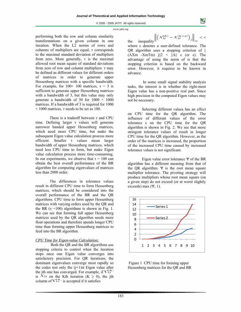
result in different CPU time to form Hessenberg matrices, which should be considered into the overall performance of the BR and the QR algorithms. CPU time to form upper Hessenberg matrices with varying orders used by the QR and the BR (т =100) algorithms is shown in Fig. 1. We can see that forming full upper Hessenberg matrices used by the QR algorithm needs more float operations and therefore spends longer CPU time than forming upper Hessenberg matrices to feed into the BR algorithm. CPU Time for Eigen-value Calculation:

Both the QR and the BR algorithms use stopping criteria to control when the iteration stops once one Eigen value converges into satisfactory precision. For QR iterations, the dominant eigenvalues converge most rapidly so the codes test only the (j+1)st Eigen value after the jth one has converged. For example, if is on the Kth iteration (K ≥ 0), the jth column of is accepted if it satisfies

the inequality where ε denotes a user-defined tolerance. The QR algorithm uses a stopping criterion of || (AXm -XmTm) j||2 < ||A|| ε (or ε). The advantage of using the norm of is that the stopping criterion is based on the backward error. However, it requires to be known in advance.

In some small signal stability analysis tasks, the interest is in whether the right-most Eigen value has a non-positive real part. Since high precision in the computed Eigen values may not be necessary.

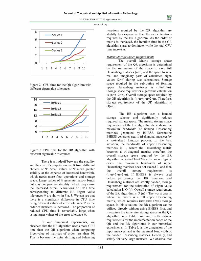
Selecting different values has an effect on CPU time for the QR algorithm. The influence of different values of the error tolerance ε on the CPU time for the QR algorithm is shown in Fig. 2. We see that more stringent tolerance values of result in longer CPU time for the QR algorithm. However, as the order of the matrices is increased, the proportion of the increased CPU time caused by increased tolerance values is not significant.

Eigen value error tolerance Ψ of the BR

algorithm has a different meaning from that of the QR algorithm. Ψ is the root mean square multiplier tolerance. The pivoting strategy will produce multipliers whose root mean square (on a given step) do not exceed (or at worst slightly exceeds) max (Ψ, 1).

02468

10121416

1 2 3 4 5 6 7 8 9 10

Series 1

Series 2

Figure 1 CPU time for forming upper Hessenberg matrices for the QR and BR



www.jatit.org

184

0

2

4

6

8

1 2 3 4 5 6 7 8 9 10

Series 1

Series 2

Series 3

Figure 2 CPU time for the QR algorithm with different eigenvalue tolerances

0

4

8

12

16

20

24

1 2 3 4 5 6 7 8 9 10

Series 1

Series 2

Series 3

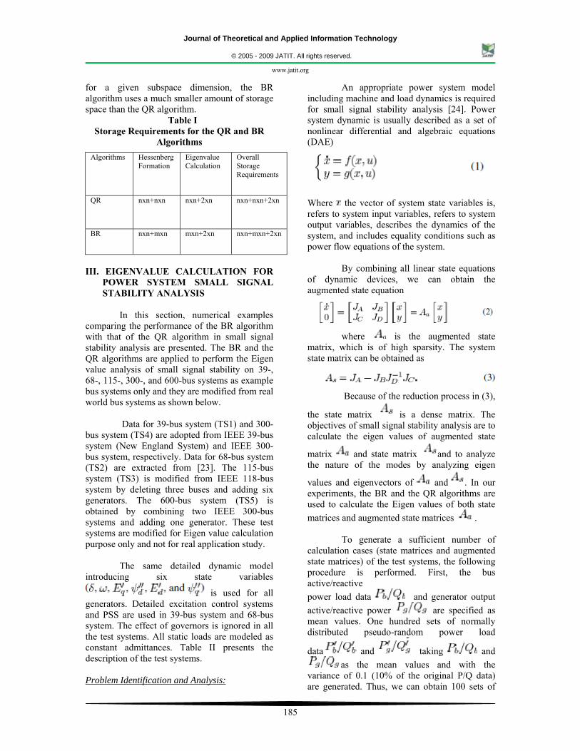
Figure 3 CPU time for the BR algorithm with different eigenvalue tolerances

There is a tradeoff between the stability and the cost of computation result from different choices of Ψ. Small values of Ψ mean greater stability at the expense of increased bandwidth, which needs more float operations and storage space. Large values of Ψ generate narrow bands but may compromise stability, which may cause the increased errors. Variations of CPU time corresponding to different BR Eigen value tolerances Ψ are shown in Fig. 3. We can see that there is a significant difference in CPU time using different values of error tolerance Ψ as the order of matrices is increased. The proportion of reduced CPU time is remarkably large when using larger values of the error tolerance Ψ.

In our numerical experiments, we

observed that the BR algorithm needs more CPU time than the QR algorithm when computing Eigenvalue of matrices of order less than 70. This is because the extra shifting and balancing

iterations required by the QR algorithm are slightly less expensive than the extra iterations required by the BR algorithm. As the order of matrix is increased, the iteration time in the QR algorithm starts to dominate, while the total CPU time increases. Matrix Storage Space Requirements

The overall Matrix storage space requirement of the QR algorithm is determined by the summation of the space to save full Hessenberg matrices (n×n) and the space to save real and imaginary parts of calculated eigen values (2×n) during two subroutines. Storage space required in the subroutine of forming upper Hessenberg matrices is (n×n+n×n). Storage space required for eigenvalue calculation is (n×n+2×n). Overall storage space required by the QR algorithm is (n×n+n×n+2×n). Therefore, storage requirement of the QR algorithm is O(n2).

The BR algorithm uses a banded

storage scheme and significantly reduces required storage space. The matrix storage space requirement of the BR algorithm depends on the maximum bandwidth of banded Hessenberg matrices generated by BHESS. Subroutine BHESS generates nearly tri-diagonal matrices by a look-ahead Lanczos process. In the best situation, the bandwidth of upper Hessenberg matrices is 1, where the Hessenberg matrix becomes a tri-diagonal matrix; therefore, the overall storage space required by the BR algorithm is (n×n+3×n+2×n). In more typical cases, the maximum bandwidth of upper Hessenberg matrices does not exceed 3, and then the overall storage requirement is (n×n+5×n+2×n). If BHESS is always used before performing the BR iteration, and Hessenberg matrices are strictly banded, storage requirement for the subroutine of Eigen value calculation is O (n). Overall storage requirement of the BR algorithm is O (n2). The worst case is where the matrix is a full upper Hessenberg matrix, which requires (n×n+n×n+2×n) storage space. In this situation, the BR algorithm can be utilized directly without using BHESS first, and it requires the same size storage space as the QR algorithm does. Table I summarizes the storage requirements for the implementation codes of the QR and the BR algorithms in our numerical experiments. In Table I, is the dimension of the input matrices, and is the maximal bandwidth of the banded Hessenberg matrices. Generally, and satisfy for very large matrices. We observe that



www.jatit.org

185

for a given subspace dimension, the BR algorithm uses a much smaller amount of storage space than the QR algorithm.

Table I Storage Requirements for the QR and BR

Algorithms

III. EIGENVALUE CALCULATION FOR

POWER SYSTEM SMALL SIGNAL STABILITY ANALYSIS

In this section, numerical examples

comparing the performance of the BR algorithm with that of the QR algorithm in small signal stability analysis are presented. The BR and the QR algorithms are applied to perform the Eigen value analysis of small signal stability on 39-, 68-, 115-, 300-, and 600-bus systems as example bus systems only and they are modified from real world bus systems as shown below.

Data for 39-bus system (TS1) and 300-

bus system (TS4) are adopted from IEEE 39-bus system (New England System) and IEEE 300-bus system, respectively. Data for 68-bus system (TS2) are extracted from [23]. The 115-bus system (TS3) is modified from IEEE 118-bus system by deleting three buses and adding six generators. The 600-bus system (TS5) is obtained by combining two IEEE 300-bus systems and adding one generator. These test systems are modified for Eigen value calculation purpose only and not for real application study.

The same detailed dynamic model introducing six state variables

is used for all generators. Detailed excitation control systems and PSS are used in 39-bus system and 68-bus system. The effect of governors is ignored in all the test systems. All static loads are modeled as constant admittances. Table II presents the description of the test systems. Problem Identification and Analysis:

An appropriate power system model including machine and load dynamics is required for small signal stability analysis [24]. Power system dynamic is usually described as a set of nonlinear differential and algebraic equations (DAE)

Where the vector of system state variables is, refers to system input variables, refers to system output variables, describes the dynamics of the system, and includes equality conditions such as power flow equations of the system.

By combining all linear state equations of dynamic devices, we can obtain the augmented state equation

where is the augmented state

matrix, which is of high sparsity. The system state matrix can be obtained as

Because of the reduction process in (3),

the state matrix is a dense matrix. The objectives of small signal stability analysis are to calculate the eigen values of augmented state

matrix and state matrix and to analyze the nature of the modes by analyzing eigen

values and eigenvectors of and . In our experiments, the BR and the QR algorithms are used to calculate the Eigen values of both state matrices and augmented state matrices .

To generate a sufficient number of

calculation cases (state matrices and augmented state matrices) of the test systems, the following procedure is performed. First, the bus active/reactive power load data and generator output active/reactive power are specified as mean values. One hundred sets of normally distributed pseudo-random power load

data and taking and as the mean values and with the

variance of 0.1 (10% of the original P/Q data) are generated. Thus, we can obtain 100 sets of

Algorithms Hessenberg Formation

Eigenvalue Calculation

Overall Storage Requirements

QR nxn+nxn nxn+2xn nxn+nxn+2xn

BR nxn+mxn mxn+2xn nxn+mxn+2xn



www.jatit.org

186

system data by replacing original active/reactive power P/Q data with randomly generated normally distributed for each test system. Then 100 state matrices and 100 augmented state matrices are generated based on the 100 sets of system data for each test system. The BR and the QR algorithms are performed on the 100 state matrices and the 100 augmented state matrices of the test systems.

In order to reduce the influence of computational environment on measured CPU time of the BR and the QR algorithms as greatly as possible, each matrix is computed ten times. The average value of ten measured CPU time is viewed as CPU time for the matrix. For each system, the average values of 100 calculated average CPU time on state matrices and augmented state matrices are viewed as CPU time for the BR and the QR algorithms on the test system.

The purpose of following this procedure

is to evaluate the performance of the BR and the QR algorithms on state matrices and augmented state matrices with reasonable variations in entries. In our experiments, we observed that some of the randomly generated active/reactive data sets are in the convergence precision range. Consequently, the same state matrices or augmented state matrices are obtained; therefore, Eigenvalue results are actually unchanged. This kind of situation does not affect CPU time needed by the BR and the QR algorithm when performing Eigen value calculation.

Seeing that MATLAB function eig is a well-known implementation of the QR algorithm adapted from LAPACK, we also apply eig function in numerical experiments for comparison purpose. Analysis of Calculated Results:

Tolerance values of forming upper Hessenberg matrices and Eigen value calculation of the BR algorithm are specified as т =100 and Ψ = 20, respectively. We found that these values can obtain the best overall performance of the BR algorithm with appropriate precision. The tolerance value of Eigen value calculation used in the QR algorithm is defined as

This value is also the convergence value of the Eigen value calculation indicating the precision of the results. The BR and the QR algorithms and MATLAB eig

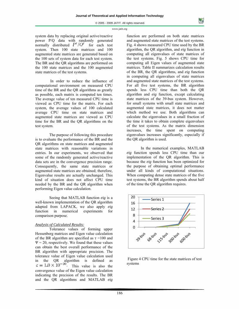
function are performed on both state matrices and augmented state matrices of the test systems. Fig. 4 shows measured CPU time used by the BR algorithm, the QR algorithm, and eig function in computing all eigenvalues of state matrices of the test systems. Fig. 5 shows CPU time for computing all Eigen values of augmented state matrices. Table II summarizes calculation results of the BR, the QR algorithms, and eig function in computing all eigenvalues of state matrices and augmented state matrices of the test systems. For all five test systems, the BR algorithm spends less CPU time than both the QR algorithm and eig function, except calculating state matrices of the 39-bus system. However, for small systems with small state matrices and augmented state matrices, it does not matter which method we use. Both algorithms can calculate the eigenvalues in a small fraction of the time it takes to obtain complete eigenvalues of the test systems. As the matrix dimension increases, the time spent on computing eigenvalues increases significantly, especially if the QR algorithm is used.

In the numerical examples, MATLAB

eig function spends less CPU time than our implementation of the QR algorithm. This is because the eig function has been optimized for the purpose of obtaining optimal performance under all kinds of computational situations. When computing dense state matrices of the five test systems, the BR algorithm spends about half of the time the QR algorithm requires.

0

4

8

12

16

20 Series 1

Series 2

Series 3

Figure 4 CPU time for the state matrices of test systems



www.jatit.org

187

0

20

40

60

80Series 1

Series 2

Series 3

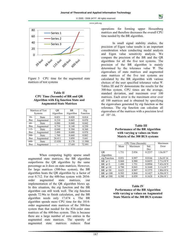
Figure 5 CPU time for the augmented state matrices of test systems

Table II CPU Time (Seconds) of BR and QR

Algorithm with Eig function State and Augmented State Matrices

Matrices of Test

Systems QR

Algorithm BR

Algorithm Eig

Function 39-Bus

State 0.021 0.020 0.014 Augmented 0.210 0.065 0.070

68-Bus

State 0.080 0.040 0.042 Augmented 0.710 0.140 0.250

115-Bus

State 0.640 0.304 0.360 Augmented 2.490 0.680 0.970

300-Bus

State 1.760 0.660 0.882 Augmented 24.411 3.050 5.641

600- Bus

State 15.850 9.170 11.980 Augmented -- 17.681 72.991

When computing highly sparse small augmented state matrices, the BR algorithm outperforms the QR algorithm by the same percentage as it does on state matrices. However, for large matrices (300-bus system), the BR algorithm beats the QR algorithm by a factor of over 0.712. For the 600-bus system with 2034-order augmented state matrices, our implementation of the QR algorithm blows up. In this situation, the eig function and the BR algorithm can still work well. The eig function spends 72.96s to finish calculation, and the BR algorithm needs only 17.674 s. The BR algorithm spends more CPU time for the 1014-order augmented state matrices of the 300-bus system than that needed for the 834-order state matrices of the 600-bus system. This is because there are a large number of zero entries in the augmented state matrices. The sparsity of augmented state matrices reduces float

operations for forming upper Hessenberg matrices and therefore decreases the overall CPU time needed by the BR algorithm.

In small signal stability studies, the precision of Eigen value results is an important consideration when conducting modal analysis and Eigen value sensitivity analysis. We compare the precision of the BR and the QR algorithms for all the five test systems. The precision of the BR algorithm is mainly determined by the tolerance value Ψ. The eigenvalues of state matrices and augmented state matrices of the five test systems are calculated by the BR algorithm with various choices of the user specified tolerance value Ψ. Tables III and IV demonstrate the results for the 300-bus system. CPU times are the average, standard deviation, and maximum over 100 matrices. Each error is the maximum error over all 100 matrices and is obtained by specifying the eigenvalues generated by eig function as the reference. The eig function can calculate all eigenvalues of the matrices with a precision level of 10^-16.

Table III Performance of the BR Algorithm

with varying ψ values on State Matrix of the 300 BUS systems

CPU Time (Seconds) Maximum

Error Mean Maximum Std. Dev

QR Algorithm

1.731 2.036 0.2237 1.0x10ֿ¹º

eig Function 0.851 0.997 0.0166 1.0x10ֿ16 BR ψ=1 8.860 8.980 0.0455 2.71x10ֿ9 BR ψ=3 1.490 1.751 0.0994 7.42x10ֿ9 BR ψ=10 0.790 0.943 0.1640 3.11x10ֿ7 BR ψ=30 0.623 0.907 0.1575 1.80x10ֿ6 BR ψ=100 0.583 0.860 0.1427 6.50x10ֿ3 BR ψ=300 0.580 0.850 0.1628 4.20x10ֿ1

Table IV

Performance of the BR Algorithm with varying ψ values on Augmented State Matrix of the 300 BUS systems



www.jatit.org

188

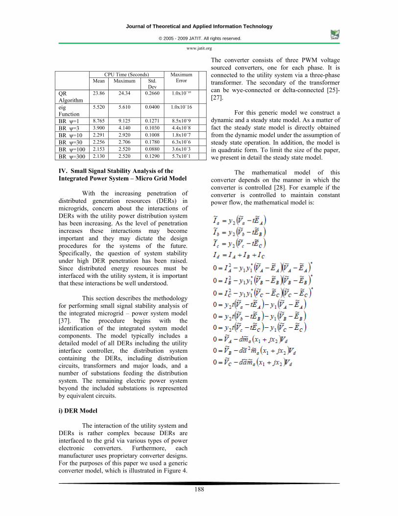
CPU Time (Seconds) Maximum

Error Mean Maximum Std.

Dev QR Algorithm

23.86 24.34 0.2660 1.0x10ֿ¹º

eig Function

5.520 5.610 0.0400 1.0x10ֿ16

BR ψ=1 8.765 9.125 0.1271 8.5x10ֿ9 BR ψ=3 3.900 4.140 0.1030 4.4x10ֿ8 BR ψ=10 2.291 2.920 0.1008 1.8x10ֿ7 BR ψ=30 2.256 2.706 0.1780 6.3x10ֿ6 BR ψ=100 2.153 2.520 0.0880 3.6x10ֿ3 BR ψ=300 2.130 2.520 0.1290 5.7x10ֿ1 IV. Small Signal Stability Analysis of the Integrated Power System – Micro Grid Model

With the increasing penetration of distributed generation resources (DERs) in microgrids, concern about the interactions of DERs with the utility power distribution system has been increasing. As the level of penetration increases these interactions may become important and they may dictate the design procedures for the systems of the future. Specifically, the question of system stability under high DER penetration has been raised. Since distributed energy resources must be interfaced with the utility system, it is important that these interactions be well understood.

This section describes the methodology

for performing small signal stability analysis of the integrated microgrid – power system model [37]. The procedure begins with the identification of the integrated system model components. The model typically includes a detailed model of all DERs including the utility interface controller, the distribution system containing the DERs, including distribution circuits, transformers and major loads, and a number of substations feeding the distribution system. The remaining electric power system beyond the included substations is represented by equivalent circuits. i) DER Model

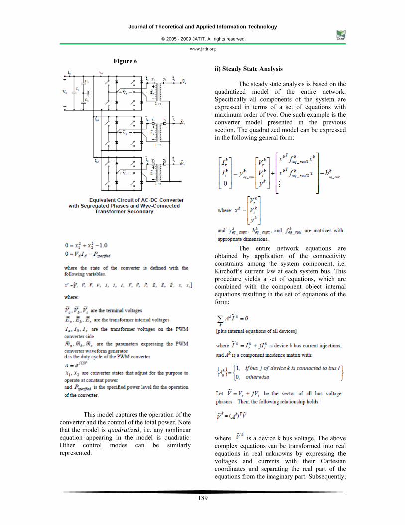
The interaction of the utility system and DERs is rather complex because DERs are interfaced to the grid via various types of power electronic converters. Furthermore, each manufacturer uses proprietary converter designs. For the purposes of this paper we used a generic converter model, which is illustrated in Figure 4.

The converter consists of three PWM voltage sourced converters, one for each phase. It is connected to the utility system via a three-phase transformer. The secondary of the transformer can be wye-connected or delta-connected [25]-[27].

For this generic model we construct a

dynamic and a steady state model. As a matter of fact the steady state model is directly obtained from the dynamic model under the assumption of steady state operation. In addition, the model is in quadratic form. To limit the size of the paper, we present in detail the steady state model.

The mathematical model of this converter depends on the manner in which the converter is controlled [28]. For example if the converter is controlled to maintain constant power flow, the mathematical model is:



www.jatit.org

189

Figure 6

This model captures the operation of the

converter and the control of the total power. Note that the model is quadratized, i.e. any nonlinear equation appearing in the model is quadratic. Other control modes can be similarly represented.

ii) Steady State Analysis

The steady state analysis is based on the quadratized model of the entire network. Specifically all components of the system are expressed in terms of a set of equations with maximum order of two. One such example is the converter model presented in the previous section. The quadratized model can be expressed in the following general form:

The entire network equations are

obtained by application of the connectivity constraints among the system component, i.e. Kirchoff’s current law at each system bus. This procedure yields a set of equations, which are combined with the component object internal equations resulting in the set of equations of the form:

where is a device k bus voltage. The above complex equations can be transformed into real equations in real unknowns by expressing the voltages and currents with their Cartesian coordinates and separating the real part of the equations from the imaginary part. Subsequently,



www.jatit.org

190

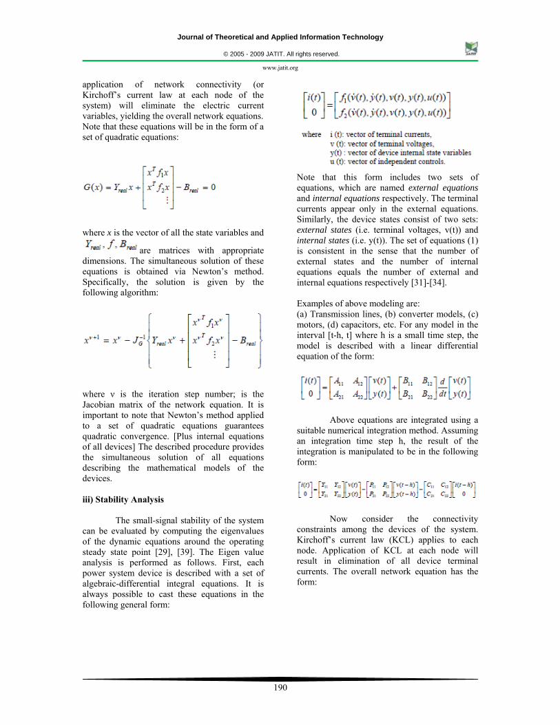
application of network connectivity (or Kirchoff’s current law at each node of the system) will eliminate the electric current variables, yielding the overall network equations. Note that these equations will be in the form of a set of quadratic equations:

where x is the vector of all the state variables and

are matrices with appropriate dimensions. The simultaneous solution of these equations is obtained via Newton’s method. Specifically, the solution is given by the following algorithm:

where ν is the iteration step number; is the Jacobian matrix of the network equation. It is important to note that Newton’s method applied to a set of quadratic equations guarantees quadratic convergence. [Plus internal equations of all devices] The described procedure provides the simultaneous solution of all equations describing the mathematical models of the devices. iii) Stability Analysis

The small-signal stability of the system can be evaluated by computing the eigenvalues of the dynamic equations around the operating steady state point [29], [39]. The Eigen value analysis is performed as follows. First, each power system device is described with a set of algebraic-differential integral equations. It is always possible to cast these equations in the following general form:

Note that this form includes two sets of equations, which are named external equations and internal equations respectively. The terminal currents appear only in the external equations. Similarly, the device states consist of two sets: external states (i.e. terminal voltages, v(t)) and internal states (i.e. y(t)). The set of equations (1) is consistent in the sense that the number of external states and the number of internal equations equals the number of external and internal equations respectively [31]-[34]. Examples of above modeling are: (a) Transmission lines, (b) converter models, (c) motors, (d) capacitors, etc. For any model in the interval [t-h, t] where h is a small time step, the model is described with a linear differential equation of the form:

Above equations are integrated using a suitable numerical integration method. Assuming an integration time step h, the result of the integration is manipulated to be in the following form:

Now consider the connectivity constraints among the devices of the system. Kirchoff’s current law (KCL) applies to each node. Application of KCL at each node will result in elimination of all device terminal currents. The overall network equation has the form:



www.jatit.org

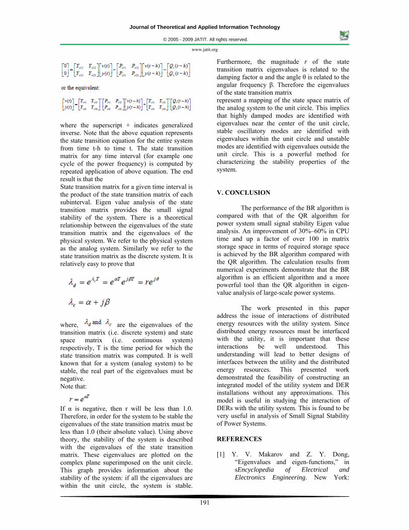
191

where the superscript + indicates generalized inverse. Note that the above equation represents the state transition equation for the entire system from time t-h to time t. The state transition matrix for any time interval (for example one cycle of the power frequency) is computed by repeated application of above equation. The end result is that the State transition matrix for a given time interval is the product of the state transition matrix of each subinterval. Eigen value analysis of the state transition matrix provides the small signal stability of the system. There is a theoretical relationship between the eigenvalues of the state transition matrix and the eigenvalues of the physical system. We refer to the physical system as the analog system. Similarly we refer to the state transition matrix as the discrete system. It is relatively easy to prove that

where, are the eigenvalues of the transition matrix (i.e. discrete system) and state space matrix (i.e. continuous system) respectively, T is the time period for which the state transition matrix was computed. It is well known that for a system (analog system) to be stable, the real part of the eigenvalues must be negative. Note that:

If α is negative, then r will be less than 1.0. Therefore, in order for the system to be stable the eigenvalues of the state transition matrix must be less than 1.0 (their absolute value). Using above theory, the stability of the system is described with the eigenvalues of the state transition matrix. These eigenvalues are plotted on the complex plane superimposed on the unit circle. This graph provides information about the stability of the system: if all the eigenvalues are within the unit circle, the system is stable.

Furthermore, the magnitude r of the state transition matrix eigenvalues is related to the damping factor α and the angle θ is related to the angular frequency β. Therefore the eigenvalues of the state transition matrix represent a mapping of the state space matrix of the analog system to the unit circle. This implies that highly damped modes are identified with eigenvalues near the center of the unit circle, stable oscillatory modes are identified with eigenvalues within the unit circle and unstable modes are identified with eigenvalues outside the unit circle. This is a powerful method for characterizing the stability properties of the system. V. CONCLUSION

The performance of the BR algorithm is compared with that of the QR algorithm for power system small signal stability Eigen value analysis. An improvement of 30%–60% in CPU time and up a factor of over 100 in matrix storage space in terms of required storage space is achieved by the BR algorithm compared with the QR algorithm. The calculation results from numerical experiments demonstrate that the BR algorithm is an efficient algorithm and a more powerful tool than the QR algorithm in eigen-value analysis of large-scale power systems.

The work presented in this paper address the issue of interactions of distributed energy resources with the utility system. Since distributed energy resources must be interfaced with the utility, it is important that these interactions be well understood. This understanding will lead to better designs of interfaces between the utility and the distributed energy resources. This presented work demonstrated the feasibility of constructing an integrated model of the utility system and DER installations without any approximations. This model is useful in studying the interaction of DERs with the utility system. This is found to be very useful in analysis of Small Signal Stability of Power Systems. REFERENCES [1] Y. V. Makarov and Z. Y. Dong,

“Eigenvalues and eigen-functions,” in sEncyclopedia of Electrical and Electronics Engineering. New York:



www.jatit.org

192

Wiley, 1998, Computational Science and Engineering, pp. 208–220.

[2] G. Henry, D. Watkins, and J. Dongarra, “A parallel implementation of the non-symmetric QR algorithm for distributed memory architectures,” SIAM J. Sci. Comput., vol. 24, no. 1, pp. 284–311, 2002.

[3] J. M. Campagnolo, N. Martins, and D. M. Falcão, “An efficient and robust eigen value method for small-signal stability assessment in parallel computers,” IEEE Trans. Power Syst., vol. 10, no. 1, pp. 506–511, Feb. 1995.

[4] D. S. Watkins and L. Elsner, Chasing algorithms for the Eigen value problem, SIAM J. Matrix Anal. Appl., 12 (1991), pp. 374–384.

[5] A. Semlyen and L. Wang, “Sequential computation of the complete Eigen system for the study zone in small signal stability analysis of large power systems,” IEEE Trans. Power Syst., vol. 3, no. 2, pp. 715–725, May 1988.

[6] L.Wang and A. Semlyen, “Application of sparse eigenvalue techniques to the small signal stability analysis of large power system,” IEEE Trans. Power Syst., vol. 5, no. 2, pp. 635–642, May 1990.

[7] D. Y. Wong, G. J. Rogers, B. Porretta, and P. Kundur, “Eigenvalue analysis of very large power systems,” IEEE Trans. Power Syst., vol. 3, no. 2, pp. 472–480, May 1988.

[8] N. Uchida and T. Nagao, “A new eigen-analysis method of steady state Stability studies for large power systems: S matrix method,” IEEE Trans. Power Syst., vol. 3, no. 2, pp. 706–714, May 1988.

[9] G. Angelidis and A. Semlyen, “Efficient calculation of critical eigenvalue clusters in the small signal stability analysis of large power systems,” IEEE Trans. Power Syst., vol. 10, no. 1, pp. 427–432, Feb. 1995.

[10] D. M. Lam, H. Yee, and B. Campbell, “An efficient improvement of the AESOPS algorithm for power system eigenvalue calculation,” IEEE Trans. Power Syst., vol. 9, no. 4, pp. 1880–1885, Nov. 1994.

[11] D. J. Stadnicki and J. E. V. Ness, “Invariant subspace method for Eigen value computation,” IEEE Trans. Power Syst., vol. 8, no. 2, pp. 572–580, May 1993.

[12] J. M. Campagnolo, N. Martins, and D. M. Falcão, “Refactored bi-iteration: A high

performance eigen solution method for large power system matrices,” IEEE Trans. Power Syst., vol. 11, no. 3, pp. 1228–1235, Aug. 1996.

[13] G. Angelidis and A. Semlyen, “Improved methodologies for the calculation of critical eigen values in small signal stability analysis,” IEEE Trans. Power Syst., vol. 11, no. 3, pp. 1209–1217, Aug. 1996.

[14] G. A. Geist, G. W. Howell, and D. S. Watkins, “The BR eigen value algorithm,” SIAM J. Matrix Anal. Appl., vol. 20, no. 4, pp. 1083–1098, Jul. 1999.

[15] P. W. Sauer, C. Raja gopalan, and M. A. Pai, “An explanation and generalization of the AESOPS and PEALS algorithms,” IEEE Trans. Power Syst., vol. 6, no. 1, pp. 293–299, Feb. 1991.

[16] D. S. Watkins, “Bulge exchanges in algorithms of QR type,” SIAM J. Matrix Anal. Appl., vol. 19, no. 4, pp. 1074 1096, Oct. 1998.

[17] D. Calvetti, S. M. Kim, and L. Reichel, “The restarted QR-algorithm for eigenvalue computation of structured matrices,” J. Comput. Appl. Math., vol. 149, pp. 415–422, 2002.

[18] D. S. Watkins, “The transmission of shifts and shift blurring in the QR algorithm,” Linear Alg. Appl., vol. 241–243, pp. 877–896, 1996.

[19] P. Kundur, G. J. Rogers, D. Y. Wong, L. Wang, and M. G. Lauby, “A comprehensive computer program package for small signal stability analysis of power systems,” IEEE Trans. Power Syst., vol. 5, no. 4, pp. 1076–1083, Nov. 1990.

[20] G. W. Howell and N. Diaa, “Algorithm 841: BHESS: Gaussian reduction to a similar banded Hessenberg form,” ACM Trans. Math. Softw., vol. 31, no. 1, pp. 166–185, Mar. 2005.

[21] W. H. Press, S. A. Teukolsky, W. T. Vetterling, and B. P. Flannery, Numerical Recipes in C: The Art of Scientific Computing, 2nd ed. New York: Cambridge Univ. Press, 1992.

[22] J. A. Scott, “An Arnoldi code for computing selected eigenvalues of sparse, real, unsymmetric matrices,” ACMTrans. Math. Softw., vol. 21, no. 4, pp. 432–475, Dec. 1995.

[23] B. Pal and B. Chaudhuri, Robust Control in Power System. New York: Springer, 2005.



www.jatit.org

193

[24] Y. V. Makarov, Z. Y. Dong, and D. J. Hill, “A general method for small signal stability analysis,” IEEE Trans. Power Syst., vol. 13, no. 3, pp. 979–985, Aug. 1998.

[25] Akira Nabae, Isao Takahashi, Hirofumi Akagi, “A New Neutral-Point-Clamped PWM Inverter”, IEEE Transaction on Industry Applications, Vol. 17, No. 5, September, 1981.

[26] Jih-Sheng Lai, Fang Zheng Peng, “Multilevel Converters – A New Breed of Power Converters”, IEEE Transaction on Industry Applications, Vol. 32, No. 3, May/June, 1996.

[27] Sakis Meliopoulos, Wenzhong Gao, Sasan Jalali, Scott Henneberry, Goerge Cokkinides, “Power Quality Assessment via Physically Based Statistical Simulation Method”.

[28]Thomas Kailath, “Linear Systems”, Prentice Hall, 1980.

[29]Yousin Tang, A. P. Sakis Meliopoulos, “Power system small signal stability analysis with 600 Bulk Power System Dynamics and Control - VI, August 22-27, 2004, Cortina d’Ampezzo, Italy FACTS elements”, IEEE Trans. of power delivery, Vol. 12, No. 3, pp. 1352-1361, July 1997.

[30] A. P. Sakis Meliopoulos, Power System Grounding and Transients: An Introduction, Marcel Dekker, 1988 (second printing). 7. CIGRE Working Group WG 37-23, “Impact of increasing contribution of dispersed generation on the power system”, 1997.

[31] R.H. Lasseter, “Control of Distributed Resources”, presented at Bulk Power System dynamics and Control IV – Restructuring, August 24 28, Santorini, Greece

[32]N.D.Hatziargyriou, T.S.Karakatsanis, “Distribution System Voltage and Reactive Power Control Based on Probabilistic Load Flow Analysis”, IEE Proc. Generation, Transmission and Distribution, Vol. 144, No. 4, July 1997, pp. 363-369.

[33] “Electricity Tariffs for Embedded Renewable Generation”, JOULE III Project JOR3-CT98- 0201, 1st Progress Report, December 1998.

[34] “Effect of high wind power penetration on the reliability and security of isolated power systems”, E.N. Dialynas, N.D.

Hatziargyriou, N. Koskolos, E. Karapidakis, paper 38-302, 37th Session, CIGRE, Paris, 30th August-5th September 1998.

[35] CIGRE TF38.01.10, “Modeling New Forms of Generation and Storage”, April 2001.

[36] A. P. Sakis Meliopoulos, G. J. Cokkinides and Robert Lasseter, “An Advanced Model for Simulation and Design of Distributed Generation Systems”, Proceedings of MedPower 2002, Athens, Greece, Nov 3-5, 2002.

[37] A. P. Sakis Meliopoulos, G. J. Cokkinides and Robert Lasseter, “A MultiPhase Power Flow Model for µGrid Analssis”, Proceedings of the 36st Annual Hawaii International Conference on System Sciences, p. 61 (pp. 1-7), Big Island, Hawaii, January 6-9, 2003

[38] Wenzhong Gao, E. Solodovnik, R. Dougal, G. J. Cokkinides and A. P. Sakis Meliopoulos, “Elimination of Numerical Oscillations in Power System Dynamic Simulation”, Proceedings of APEC 2003, pp. 790-794, Miami, FL, Feb 9-13,

2003. [39] Deok Young Kim and A. P. Sakis

Meliopoulos, “Comparison of Small Signal Stability Analysis Methods in Complex Systems with Switching Elements”, Proceedings of IFAC 2003, pp 1292-1296, Seoul, Korea, September 15-19, 2003.

[40] Sakis Meliopoulos, “Challenges in Simulation and Design of Micro Grids”, Proceedings of the 2002 IEEE/PES Winter Meeting, New York, NY, Jan 28-31, 2002.

[41] G. H. Golub and C. F. Van Loan, Matrix Computations, 3rd ed. Baltimore, MD: John Hopkins Univ. Press, 1996.



www.jatit.org

194

EIGEN VALUE TECHNIQUES FOR SMALL SIGNAL STABILITY ANALYSIS ... · PDF fileEIGEN VALUE TECHNIQUES FOR SMALL SIGNAL STABILITY ANALYSIS IN POWER SYSTEM STABILITY ... research for small

Documents