EFH Calculation

EFH – Equivalent Flat Haul

Efficiency Measure and Planning Tool

Definition

• EFH – Equivalent Flat Haul. The theoretical equivalent distance a truck could travel in the same time on a flat haul road.

Application• For each grade, divide the flat haul speed by the

speed on grade. For example, if the flat haul speed is 40km/hr and the average speed on a 10% ramp is 10km/hr, then the EFH factor for any 10% ramp is 40/10 or 4.

• The horizontal distance of each road segment is multiplied by the EFH factor for that segment. For Example if the 10% road segment from above was 500m long, then the Equivalent Flat Haul for that segment of road would be 500 x 4 or 2000m.

Example – Case 1

Dist = 2km

EFH = 40/40 * 1

= 2 km

Dist = 1km

EFH = 40/10 * 1

= 4km

Dist = 1 + 2 + 1 = 4km

EFH Speed = 40km/hrCycle Time = 10/(40/60) = 15 min.

Average Speed =

4 / (15/60) = 16km/hr

40 km/hr10 km/hr

10 km/hr

Dist = 1km

EFH = 40/10 * 1

= 4km

EFH = 4 + 2 + 4 = 10km

Example – Case 2

Dist = 2km

EFH = 40/40 * 1

= 2 km

Dist = 1km

EFH = 40/10 * 1

= 4km

Dist = 1 + 2 + 1 = 4km

EFH Speed = 40 km/hrCycle Time = 7/(40/60) = 10.5 min.

Average Speed =

4/(10.5/60) = 22.9 km/hr

40 km/hr10 km/hr

40 km/hr

Dist = 1km

EFH = 40/40 * 1

= 1km

EFH = 4 + 2 + 1 = 7km

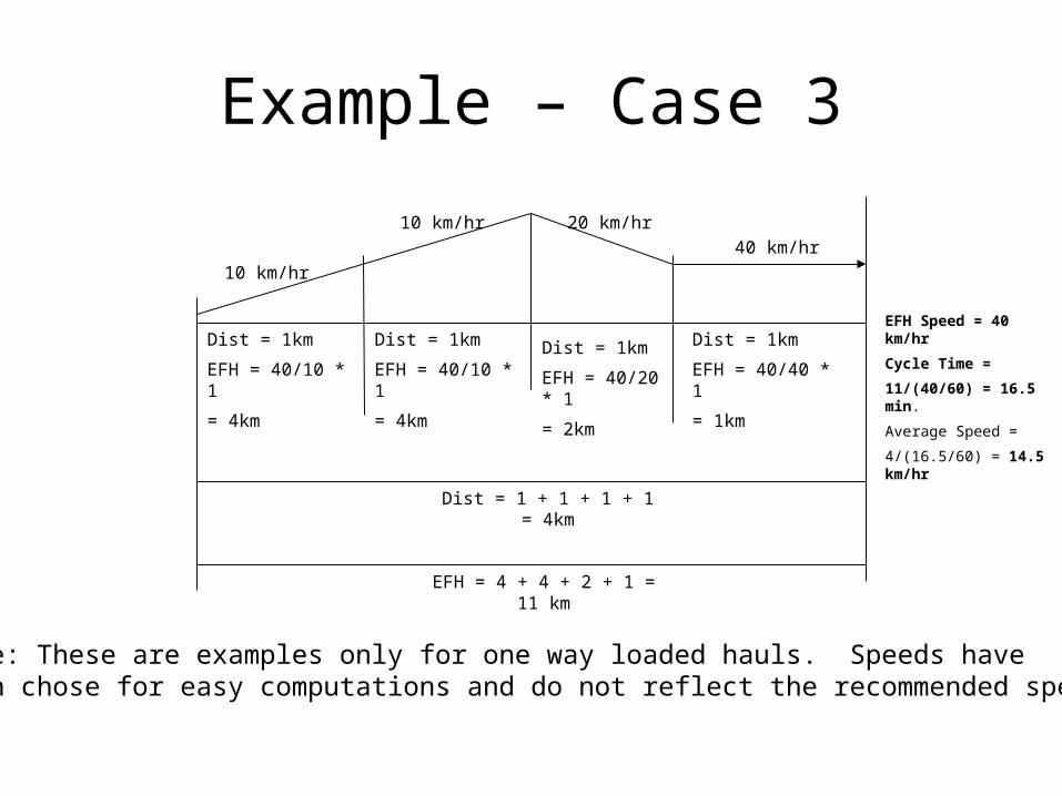
Example – Case 3

Dist = 1km

EFH = 40/10 * 1

= 4km

Dist = 1 + 1 + 1 + 1 = 4km

EFH Speed = 40 km/hrCycle Time = 11/(40/60) = 16.5 min.

Average Speed =

4/(16.5/60) = 14.5 km/hr

10 km/hr40 km/hr

Dist = 1km

EFH = 40/40 * 1

= 1km

EFH = 4 + 4 + 2 + 1 = 11 km

20 km/hr10 km/hr

Dist = 1km

EFH = 40/10 * 1

= 4km

Dist = 1km

EFH = 40/20 * 1

= 2km

Note: These are examples only for one way loaded hauls. Speeds havebeen chose for easy computations and do not reflect the recommended speeds

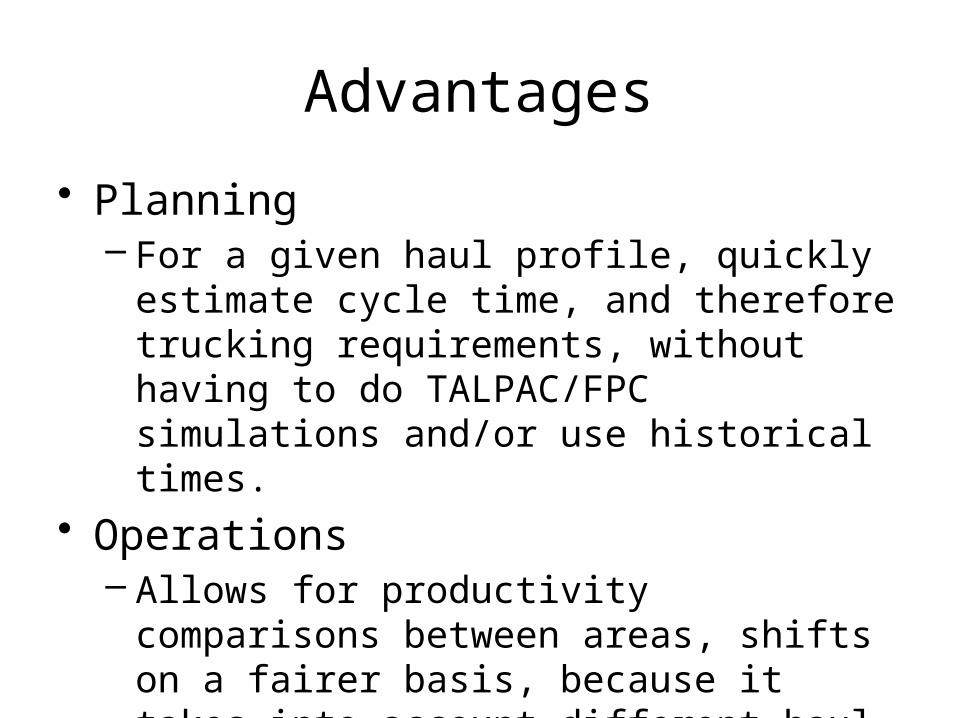
Advantages

• Planning– For a given haul profile, quickly estimate cycle

time, and therefore trucking requirements, without having to do TALPAC/FPC simulations and/or use historical times.

• Operations– Allows for productivity comparisons between

areas, shifts on a fairer basis, because it takes into account different haul profiles.

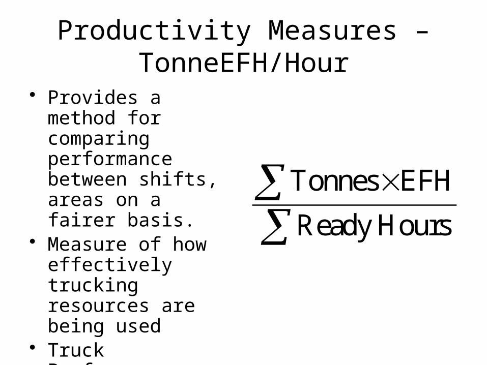
Productivity Measures – TonneEFH/Hour

• Provides a method for comparing performance between shifts, areas on a fairer basis.

• Measure of how effectively trucking resources are being used

• Truck Performance Graph

Tonnes EFHReady Hours

Truck Performance Graph – Month to Date

01/09

/2003

03/09

/2003

05/09

/2003

07/09

/2003

09/09

/2003

11/09

/2003

13/09

/2003

15/09

/2003

17/09

/2003

19/09

/2003

21/09

/2003

23/09

/2003

25/09

/2003

27/09

/2003

29/09

/2003

01/10

/2003

0

10

20

30

40

50

60

70

80

0

500

1000

1500

2000

2500

3000

Minera Yanacocha Haulage Fleet Efficiency Factors - Combined Cat 785C

Guardia 1 Wait% Guardia 2 Wait% Guardia 3 Wait%Guardia 4 Wait% Average Wait% Guardia 1 EKM/HrGuardia 2 EKM/Hr Guardia 3 EKM/Hr Guardia 4 EKM/HrAverage EKM/Hr Guardia 1 EFH Guardia 2 EFHGuardia 3 EFH Guardia 4 EFH Average EFH

Wai

t%,K

M(E

FH),K

M/H

r(EFH

)

Tonn

eKilo

met

res/

Hour

(EFH

)

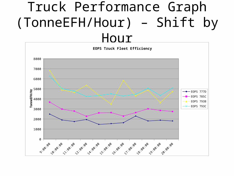
Truck Performance Graph (TonneEFH/Hour) – Shift by Hour

9:00:0

0

10:00

:00

11:00

:00

12:00

:00

14:00

:00

15:00

:00

16:00

:00

17:00

:00

18:00

:00

19:00

:00

20:00

:000

1000

2000

3000

4000

5000

6000

7000

8000

EOPS Truck Fleet Efficiency

EOPS 777D

EOPS 785C

EOPS 793B

EOPS 793CTonn

eEFH

/Hr

Productivity Measures –EFH

• Relative Haul Distances

Truck Performance Graph (EFH) – Shift by Hour

9:00:0

0

10:00

:00

11:00

:00

12:00

:00

14:00

:00

15:00

:00

16:00

:00

17:00

:00

18:00

:00

19:00

:00

20:00

:000

2

4

6

8

10

12

14

16

EOPS EFH

EOPS 777D

EOPS 785C

EOPS 793B

EOPS 793CKilo

met

res

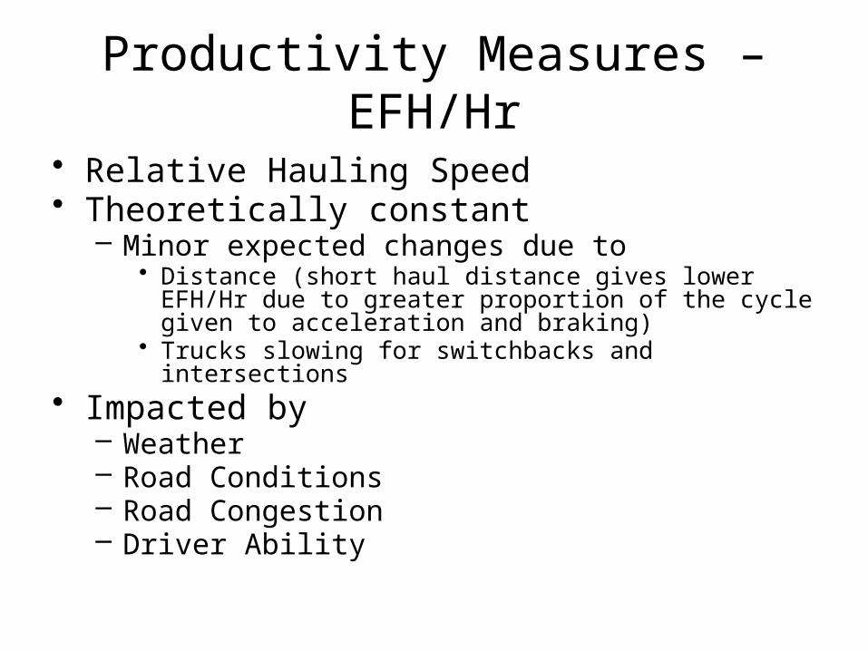
Productivity Measures –EFH/Hr• Relative Hauling Speed• Theoretically constant

– Minor expected changes due to • Distance (short haul distance gives lower EFH/Hr due to

greater proportion of the cycle given to acceleration and braking)

• Trucks slowing for switchbacks and intersections• Impacted by

– Weather– Road Conditions– Road Congestion– Driver Ability

Truck Performance Graph (EFH/Hr) – Shift by Hour

9:00:0

0

10:00

:00

11:00

:00

12:00

:00

14:00

:00

15:00

:00

16:00

:00

17:00

:00

18:00

:00

19:00

:00

20:00

:000

10

20

30

40

50

60

EOPS EFH/Hr

EOPS 777D

EOPS 785C

EOPS 793B

EOPS 793C

KM

/Hr

Productivity Measures – Wait Factor

Truck Wait Time(Truck Load Time + Truck Spot Time)

• Measure of average number of trucks in queue.

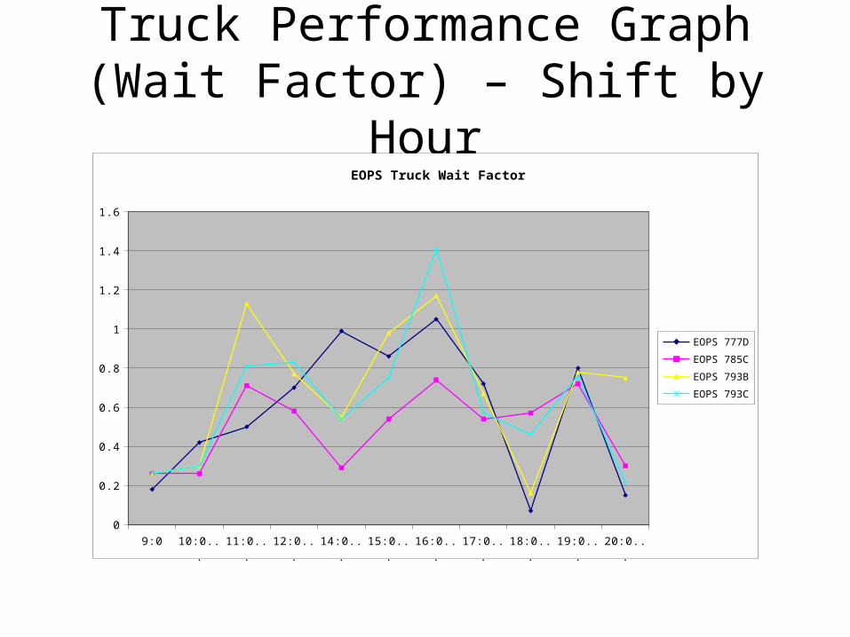
Truck Performance Graph (Wait Factor) – Shift by Hour

9:00:00 10:00:00 11:00:00 12:00:00 14:00:00 15:00:00 16:00:00 17:00:00 18:00:00 19:00:00 20:00:000

0.2

0.4

0.6

0.8

1

1.2

1.4

1.6

EOPS Truck Wait Factor

EOPS 777D

EOPS 785C

EOPS 793B

EOPS 793C

Causes for Errors in EFH Reporting

• Main causes for erroneous/misleading reporting of EFH are:– Errors in Dispatch Road Network.

• Error in X, Y give error in distance• Error in Z gives error in haul profile

– Fundamental shift in modelled speed versus road grade.

Dispatch Road Network• Needs to be checked daily• Responsibility rests within the Engineering

Group• Dispatchers should only be making minor

adjustments to loading locations and dumping points, X,Y co-ordinate changes only.

• Ramps and Drop Cuts need to be designed and built to design.

Calculation

• Determine what are appropriate speeds for various grades.– Truck Rim-pull/Retarder Curves– GPS Speed Monitoring Locations

• Function of empty/loaded and up/down

EFH Functions• Loaded Function

– Grade < -4.5%• EFH Factor = (Grade/100)*27

– Grade > 0%• EFH Factor = 1 + ((Grade/100)*35)

– Grade >= -4.5 and <=0 • EFH Factor = 1

• Empty Function– Grade < -4.5%

• EFH Factor = 0.75 + ((Grade/100)*8.5)– Grade > +4.5%

• EFH Factor = 0.35 + ((Grade/100)*16)– Grade >= -4.5% and <= +4.5%

• EFH Factor = 1

Modelled Speed Vs Grade

-11 -10 -9 -8 -7 -6 -5 -4 -3 -2 -1 0 1 2 3 4 5 6 7 8 9 10 110.0

10.0

20.0

30.0

40.0

50.0

60.0

Loaded SpeedEmpty Speed

Road Grade (%)

Trav

el S

peed

(KM

/Hr)

Shift in Modelled Speed Versus Grade

• Monitor real travel speeds on differing ramp grades– Road Condition Report

• If a significant shift is noticed, the EFH calculation needs to be adjusted– Needs to be agreed to between Planning and

Operations– Changes need to be done in a way that

preserves value of historical data

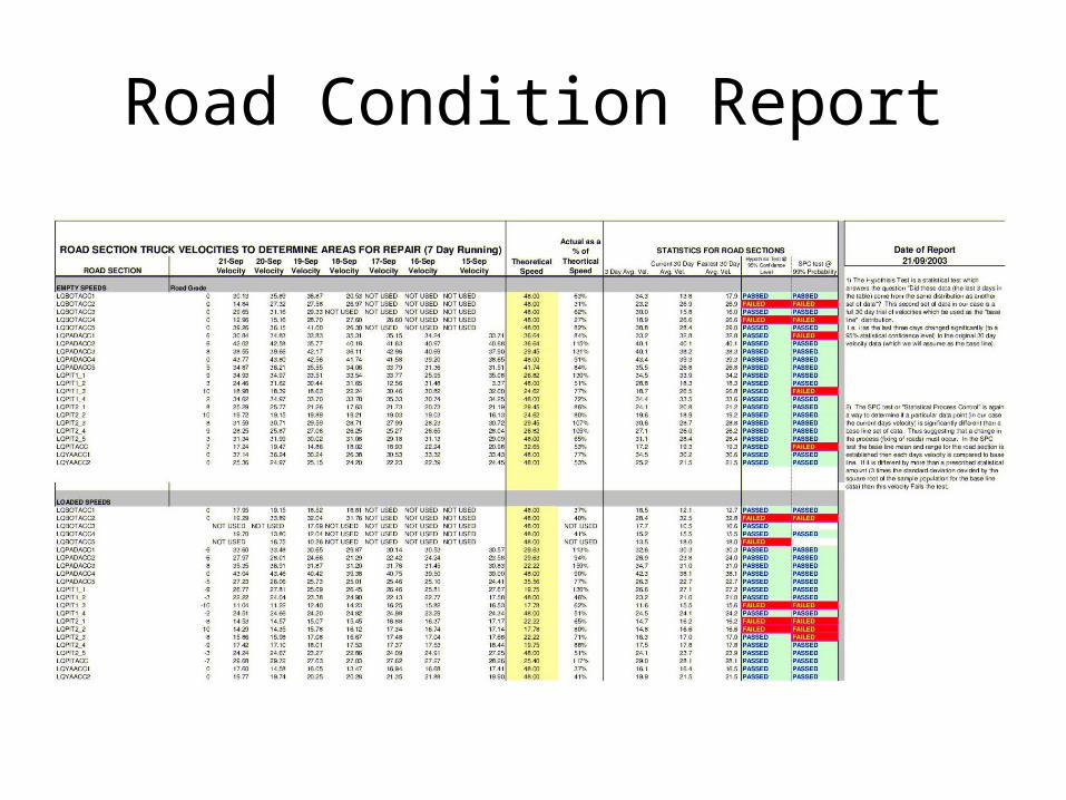
Road Condition Report