Efficient Signal, Code, and Receiver Designs for MIMO Communication Systems by Huan Yao B.S. Physics, B.S. Electrical Science and Engineering Massachusetts Institute of Technology, 1997 M.Eng. Electrical Engineering and Computer Science Massachusetts Institute of Technology, 1998 Submitted to the Department of Electrical Engineering and Computer Science in partial fulfillment of the requirements for the degree of Doctor of Philosophy in Electrical Engineering and Computer Science at the MASSACHUSETTS INSTITUTE OF TECHNOLOGY June 2003 c Massachusetts Institute of Technology 2003. All rights reserved. Author .............................................................. Department of Electrical Engineering and Computer Science May 21, 2003 Certified by .......................................................... Gregory W. Wornell Professor Thesis Supervisor Accepted by ......................................................... Arthur C. Smith Chairman, Department Committee on Graduate Students

Welcome message from author
This document is posted to help you gain knowledge. Please leave a comment to let me know what you think about it! Share it to your friends and learn new things together.
Transcript
Efficient Signal, Code, and Receiver Designs
for MIMO Communication Systems
by
Huan Yao
B.S. Physics, B.S. Electrical Science and EngineeringMassachusetts Institute of Technology, 1997
M.Eng. Electrical Engineering and Computer ScienceMassachusetts Institute of Technology, 1998
Submitted to the Department of Electrical Engineering and ComputerScience
in partial fulfillment of the requirements for the degree of
Doctor of Philosophy in Electrical Engineering and Computer Science
at the
MASSACHUSETTS INSTITUTE OF TECHNOLOGY
June 2003
c© Massachusetts Institute of Technology 2003. All rights reserved.
Author . . . . . . . . . . . . . . . . . . . . . . . . . . . . . . . . . . . . . . . . . . . . . . . . . . . . . . . . . . . . . .Department of Electrical Engineering and Computer Science
May 21, 2003
Certified by. . . . . . . . . . . . . . . . . . . . . . . . . . . . . . . . . . . . . . . . . . . . . . . . . . . . . . . . . .Gregory W. Wornell
ProfessorThesis Supervisor
Accepted by . . . . . . . . . . . . . . . . . . . . . . . . . . . . . . . . . . . . . . . . . . . . . . . . . . . . . . . . .Arthur C. Smith
Chairman, Department Committee on Graduate Students

2
Efficient Signal, Code, and Receiver Designs
for MIMO Communication Systems
by
Huan Yao
Submitted to the Department of Electrical Engineering and Computer Scienceon May 21, 2003, in partial fulfillment of the
requirements for the degree ofDoctor of Philosophy in Electrical Engineering and Computer Science
Abstract
The so-called diversity-multiplexing tradeoff characterizes the fundamental interac-tion between the robustness and capacity gains obtainable from multiple-input andmultiple-output (MIMO) systems in fading environments. This thesis develops prac-tical schemes for approaching the optimal tradeoff in various delay and complexityregimes. We focus on a two-transmit and two-receive antenna system, in which thereceiver has channel knowledge, but the transmitter does not.
We first investigate uncoded transmission. We propose a class of lattice-reduction-aided low-complexity detectors that can achieve near maximum likelihood perfor-mance and the best diversity-multiplexing tradeoff achievable by any length-one code.
We also design a family of structured space-time block codes that we call tilted-QAM codes. It achieves the optimal infinite-delay tradeoff with the necessary mini-mum delay of two, answering a previously open question. It uses constellation rotationideas to effectively spread information across space and time. We identify rotationangles that are universally optimal at all rates in terms of a determinant criterion.
We further develop efficient coding schemes using long error correction codes.In particular, we combine them with tilted-QAM codes using hard and soft deci-sion decoding to obtain good performance at moderate SNR. These new systems arecompared to orthogonal space-time coded systems, which we show to achieve near op-timal performance at low SNR. We also examine traditional sequential versions anddevelop new block versions of the Bell Labs layered architecture (BLAST). Whilesome of these can in principle reach the performance limit at all SNRs, we show theyalso have various practical problems.
Finally, for the case where no channel knowledge is available, we present a ge-ometric view of the signal design problem. This view reveals how training basedapproaches can achieve the optimal (non-coherent) diversity-multiplexing tradeoff.
Thesis Supervisor: Gregory W. WornellTitle: Professor
3

4

Acknowledgments
First of all, I would like to thank my thesis supervisor Prof. Greg Wornell. He took
me under his wing six years ago, and taught me much. I can feel it. He is brilliant,
knowledgeable, insightful, and most importantly, always available. I thank him for
guiding me to learn the art of research and the philosophy behind it. Although there
were times when I did not feel this way, I am now thankful that he did not tell
me exactly what to do and allowed me to develop my own ideas. I have enjoyed
the personal interactions. I feel very lucky to have an adviser as humorous as him.
Greg, you’re a funny guy.
I would also like to express my deepest gratitude toward the other members of
my committee, Prof. Lizhong Zheng and Prof. Muriel Medard, for the many helpful
discussions throughout the course of the thesis. Lizhong’s own Ph.D. thesis and
further conversations with him sparked many ideas in this thesis. Muriel’s broader
perspective helped raising new questions and understanding various facets of the
problem. My mentor at AT&T Labs Dr. Rick Rose and my academic adviser Prof.
Dave Forney provided me with advise and guidance over the years. For that, I
sincerely thank them.
I thank all members of the DSP group for making it a second home for me. In par-
ticular, I would like to thank Albert Chan, Nick Laneman, Mike Lopez, Stark Draper,
Emin Martinian, Everest Huang, Uri Erez, and Charles Sestok, for the numerous
technical discussions, the interesting water-cooler chats, and the fun conference trips
together.
Let me take this opportunity to acknowledge the generous financial support from
the National Science Foundation Graduate Research Fellowship Program, the AT&T
Labs Fellowship Program, as well as HP through the HP/MIT Alliance, TI through
the Leadership Universities Program, NSF under Grant No. CCR-9979363, Army
Research Laboratory under Collaborative Technology Alliance No. DAAD19-01-2-
0011, and MARCO/DARPA C2S2 under Contract No. 2001-CT-888.
I thank all my friends for their support and the enjoyable times we had together,
5

Alice Wang, the Li’s (Li Lee and Li Shu), Angela Lin, Justine Song, Irina Medvedev,
Anna Lysyanskaya, and many wonderful people I met at Ashdown. They made my
life at MIT more complete. Special thanks to Alice: We have been at MIT and many
of the summer internships together for the past ten years. I know I have thanked her
in all my previous theses. Thanks again for the last five years.
One thousand thanks to Tairan Wang, my husband-to-be in a few weeks. I don’t
think I can thank him enough. This thesis would not be the way it is without him.
He was the first sounding board for many of my key ideas. Talking to him helps
me think. And those quick MATLAB scripts for testing my ideas certainly came in
handy. All these are on top of being a good friend and supporter throughout the ups
and downs on this long Ph.D road.
Finally, I would like to thank my parents and my big brother for their never-
ending love and support. They left their lives in China behind and immigrated to
this country so that I could receive top-grade education and lead a good life. It can
finally start to pay off now. I hope the hooding ceremony will be a nice treat!
6
Contents
1 Introduction 19
1.1 Channel and System Model . . . . . . . . . . . . . . . . . . . . . . . 20
1.2 Thesis Outline . . . . . . . . . . . . . . . . . . . . . . . . . . . . . . . 23
2 Theoretical Background 27
2.1 Channel Capacity and Outage Probability . . . . . . . . . . . . . . . 27
2.2 Visualizing Rate and Robustness Gains . . . . . . . . . . . . . . . . . 28
2.3 Diversity-Multiplexing Tradeoff . . . . . . . . . . . . . . . . . . . . . 31
2.3.1 Definitions . . . . . . . . . . . . . . . . . . . . . . . . . . . . . 31
2.3.2 Optimal Tradeoff Results . . . . . . . . . . . . . . . . . . . . . 32
2.3.3 Two-Transmit Two-Receive Antenna Case . . . . . . . . . . . 34
2.3.4 Visualizing The Tradeoff . . . . . . . . . . . . . . . . . . . . . 37
2.3.5 Local Diversity-Multiplexing Tradeoff . . . . . . . . . . . . . . 40
2.4 Error Probability and Design Criteria . . . . . . . . . . . . . . . . . . 41
2.5 Performance of Gaussian Random Codes . . . . . . . . . . . . . . . . 45
2.5.1 Tradeoff Achieved . . . . . . . . . . . . . . . . . . . . . . . . . 46
2.5.2 Worst-Pair Bound . . . . . . . . . . . . . . . . . . . . . . . . . 47
3 Uncoded Systems and Efficient Detection 51
3.1 Introduction . . . . . . . . . . . . . . . . . . . . . . . . . . . . . . . . 51
3.2 Traditional Detectors . . . . . . . . . . . . . . . . . . . . . . . . . . . 52
3.3 Lattice Reduction . . . . . . . . . . . . . . . . . . . . . . . . . . . . . 56
3.3.1 Choice of optimal basis . . . . . . . . . . . . . . . . . . . . . . 57
7
3.3.2 Reduction Algorithm . . . . . . . . . . . . . . . . . . . . . . . 59
3.3.3 Convergence and Complexity . . . . . . . . . . . . . . . . . . 61
3.4 Gaussian Channels . . . . . . . . . . . . . . . . . . . . . . . . . . . . 64
3.4.1 Complexity . . . . . . . . . . . . . . . . . . . . . . . . . . . . 64
3.4.2 Performance . . . . . . . . . . . . . . . . . . . . . . . . . . . . 64
3.5 Rayleigh Fading Channels . . . . . . . . . . . . . . . . . . . . . . . . 67
3.5.1 Complexity . . . . . . . . . . . . . . . . . . . . . . . . . . . . 67
3.5.2 Performance . . . . . . . . . . . . . . . . . . . . . . . . . . . . 67
3.5.3 Diversity-Multiplexing Tradeoff . . . . . . . . . . . . . . . . . 70
3.6 Lattice Reduction at Transmitter . . . . . . . . . . . . . . . . . . . . 72
3.7 Higher Dimensional Lattice Reduction . . . . . . . . . . . . . . . . . 76
3.7.1 Existing Algorithms . . . . . . . . . . . . . . . . . . . . . . . 76
3.7.2 Complexity and Performance of LLL . . . . . . . . . . . . . . 79
3.8 Summary . . . . . . . . . . . . . . . . . . . . . . . . . . . . . . . . . 82
4 Structured Codes with Minimum Delay 85
4.1 Introduction . . . . . . . . . . . . . . . . . . . . . . . . . . . . . . . . 85
4.2 OSTBC . . . . . . . . . . . . . . . . . . . . . . . . . . . . . . . . . . 86
4.2.1 The Smart Repetition . . . . . . . . . . . . . . . . . . . . . . 87
4.2.2 Theoretical Performance Analysis . . . . . . . . . . . . . . . . 87
4.2.3 Simulation Results . . . . . . . . . . . . . . . . . . . . . . . . 89
4.3 Tilted-QAM Code . . . . . . . . . . . . . . . . . . . . . . . . . . . . 90
4.3.1 The Rotation Design . . . . . . . . . . . . . . . . . . . . . . . 90
4.3.2 Choice of rotation angles . . . . . . . . . . . . . . . . . . . . . 92
4.4 Theoretical Performance Analysis . . . . . . . . . . . . . . . . . . . . 95
4.4.1 Minimum Distance Property . . . . . . . . . . . . . . . . . . . 97
4.4.2 Determinant Counting . . . . . . . . . . . . . . . . . . . . . . 101
4.4.3 Determinant Counting: Higher Dimensional Cases . . . . . . . 103
4.5 Simulation Results . . . . . . . . . . . . . . . . . . . . . . . . . . . . 106
4.5.1 ML/Sphere Decoding . . . . . . . . . . . . . . . . . . . . . . . 107
8
4.5.2 Lattice Decoding . . . . . . . . . . . . . . . . . . . . . . . . . 109
4.6 Tilted-QAM in Single Antenna Case . . . . . . . . . . . . . . . . . . 110
4.6.1 Channel Model and Theoretical Background . . . . . . . . . . 111
4.6.2 Tilted-QAM design . . . . . . . . . . . . . . . . . . . . . . . . 113
4.6.3 Error Probability Evaluation . . . . . . . . . . . . . . . . . . . 114
4.7 Summary . . . . . . . . . . . . . . . . . . . . . . . . . . . . . . . . . 117
5 Error Correction Code Enhanced Systems 119
5.1 Introduction . . . . . . . . . . . . . . . . . . . . . . . . . . . . . . . . 119
5.2 OSTBC . . . . . . . . . . . . . . . . . . . . . . . . . . . . . . . . . . 121
5.2.1 Equivalent channel . . . . . . . . . . . . . . . . . . . . . . . . 122
5.2.2 Achievable Performance . . . . . . . . . . . . . . . . . . . . . 123
5.3 Diagonal-BLAST . . . . . . . . . . . . . . . . . . . . . . . . . . . . . 126
5.3.1 Layered Encoding . . . . . . . . . . . . . . . . . . . . . . . . . 126
5.3.2 Layered Decoding . . . . . . . . . . . . . . . . . . . . . . . . . 128
5.3.3 D-BLAST Caveats . . . . . . . . . . . . . . . . . . . . . . . . 132
5.3.4 Experimental Setup . . . . . . . . . . . . . . . . . . . . . . . . 138
5.3.5 Simulation Results . . . . . . . . . . . . . . . . . . . . . . . . 141
5.4 Modified BLAST in Block Form . . . . . . . . . . . . . . . . . . . . . 143
5.4.1 Code Designs . . . . . . . . . . . . . . . . . . . . . . . . . . . 144
5.4.2 Multiple Access Channel Framework . . . . . . . . . . . . . . 146
5.4.3 V-BLAST . . . . . . . . . . . . . . . . . . . . . . . . . . . . . 151
5.4.4 Two-Layer-D-BLAST . . . . . . . . . . . . . . . . . . . . . . . 154
5.4.5 X-BLAST . . . . . . . . . . . . . . . . . . . . . . . . . . . . . 157
5.4.6 Comparisons . . . . . . . . . . . . . . . . . . . . . . . . . . . 159
5.5 Tilted-QAM With Hard-Decision ECC . . . . . . . . . . . . . . . . . 163
5.5.1 System Setup . . . . . . . . . . . . . . . . . . . . . . . . . . . 164
5.5.2 Simulation Results . . . . . . . . . . . . . . . . . . . . . . . . 165
5.6 Tilted-QAM with Soft-Decision ECC . . . . . . . . . . . . . . . . . . 167
5.6.1 System Setup . . . . . . . . . . . . . . . . . . . . . . . . . . . 168
9
5.6.2 Iterative Soft-Decision Decoder . . . . . . . . . . . . . . . . . 169
5.6.3 Simulation Results . . . . . . . . . . . . . . . . . . . . . . . . 173
5.7 Summary . . . . . . . . . . . . . . . . . . . . . . . . . . . . . . . . . 175
6 Non-Coherent Communications 177
6.1 Theoretical Background . . . . . . . . . . . . . . . . . . . . . . . . . 178
6.1.1 Capacity . . . . . . . . . . . . . . . . . . . . . . . . . . . . . . 178
6.1.2 Capacity Achieving Distribution . . . . . . . . . . . . . . . . . 180
6.2 Non-Coherent Communication Signal Design . . . . . . . . . . . . . . 181
6.2.1 Design Criterion . . . . . . . . . . . . . . . . . . . . . . . . . 182
6.2.2 Existing Schemes . . . . . . . . . . . . . . . . . . . . . . . . . 183
6.3 Geometric Approach . . . . . . . . . . . . . . . . . . . . . . . . . . . 185
6.3.1 Projection Matrices . . . . . . . . . . . . . . . . . . . . . . . . 185
6.3.2 Embedding on Spheres . . . . . . . . . . . . . . . . . . . . . . 186
6.3.3 Signal Design . . . . . . . . . . . . . . . . . . . . . . . . . . . 187
6.3.4 Relationship to Training . . . . . . . . . . . . . . . . . . . . . 189
6.4 Channel Training Approach . . . . . . . . . . . . . . . . . . . . . . . 190
6.4.1 Quality of Channel Estimation . . . . . . . . . . . . . . . . . . 191
6.4.2 Effect of Imperfect Channel Knowledge . . . . . . . . . . . . . 192
7 Summary and Future Directions 195
7.1 Contributions . . . . . . . . . . . . . . . . . . . . . . . . . . . . . . . 195
7.2 Future Directions . . . . . . . . . . . . . . . . . . . . . . . . . . . . . 198
7.2.1 Coherent Communications . . . . . . . . . . . . . . . . . . . . 198
7.2.2 Non-coherent Communications . . . . . . . . . . . . . . . . . . 199
10
List of Figures
1-1 Multiple antenna channel with Nt transmit and Nr receive antennas. 20
2-1 Using multiple antennas allows increased data rate. . . . . . . . . . . 30
2-2 Using multiple antennas allows increased robustness or diversity. . . . 30
2-3 Optimal diversity-multiplexing tradeoff curve dout(r) for a system with
Nt transmit antennas and Nr receive antennas. . . . . . . . . . . . . 33
2-4 Optimal diversity-multiplexing tradeoff curve dout(r) for the two-transmit
two-receive antenna case. . . . . . . . . . . . . . . . . . . . . . . . . 35
2-5 Family of outage probability curves as functions of SNR for various
target rates R in the Nt = Nr = 2 case. . . . . . . . . . . . . . . . . 38
2-6 As rate grows with SNR, i.e., R = r log2(SNR), outage probability
Pout(R, SNR) decays with SNR with slope d(r). . . . . . . . . . . . . 38
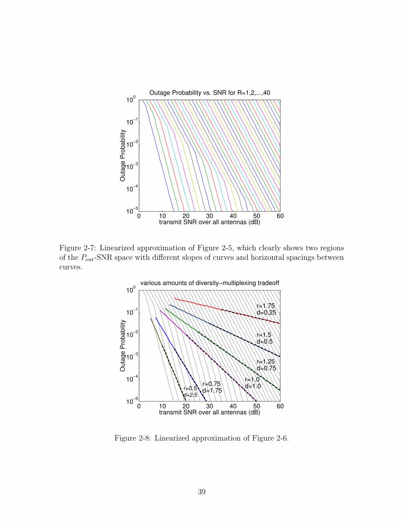
2-7 Linearized approximation of Figure 2-5, which clearly shows two re-
gions of the Pout-SNR space with different slopes of curves and hori-
zontal spacings between curves. . . . . . . . . . . . . . . . . . . . . . 39
2-8 Linearized approximation of Figure 2-6. . . . . . . . . . . . . . . . . . 39
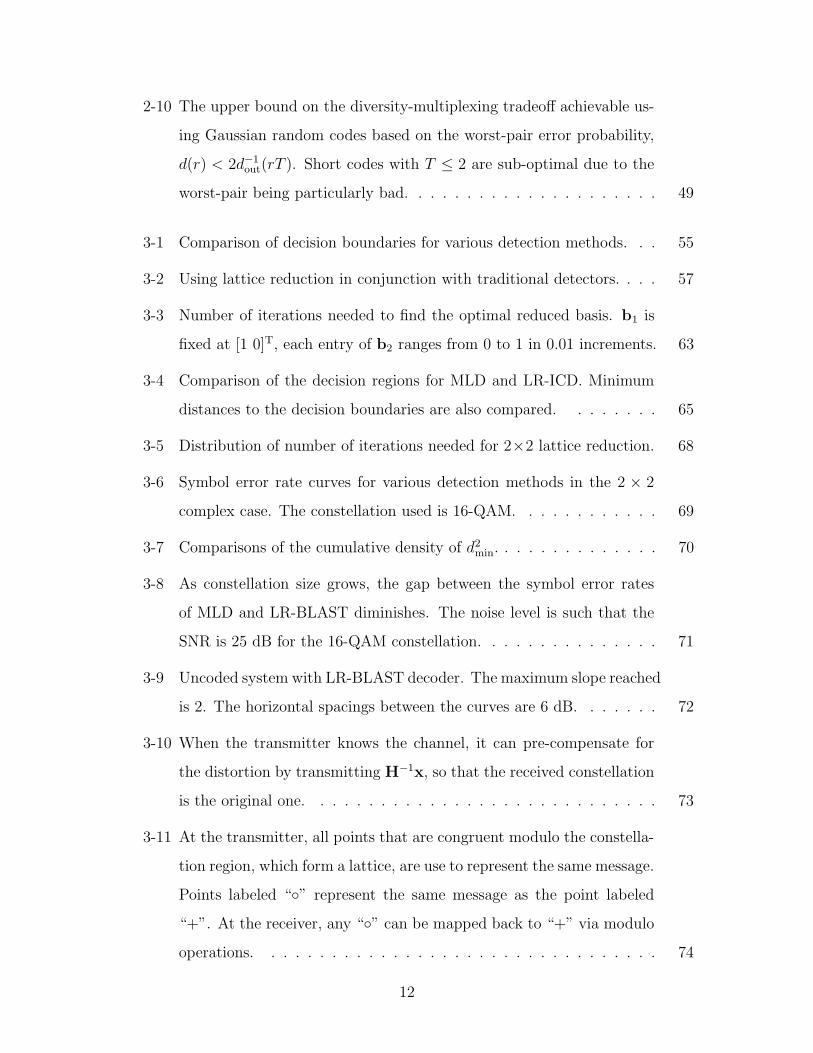
2-9 Diversity-multiplexing tradeoff achieved using Gaussian random codes
of various lengths. Optimal tradeoff is achieved with T ≥ 3. T = 2
codes (with expurgation) can achieve the end points, but is sub-optimal
for 0 < r < 1. T = 1 codes only achieve a maximum diversity of d = 2
when r = 0, which is the most any length one code can do. . . . . . 47
11
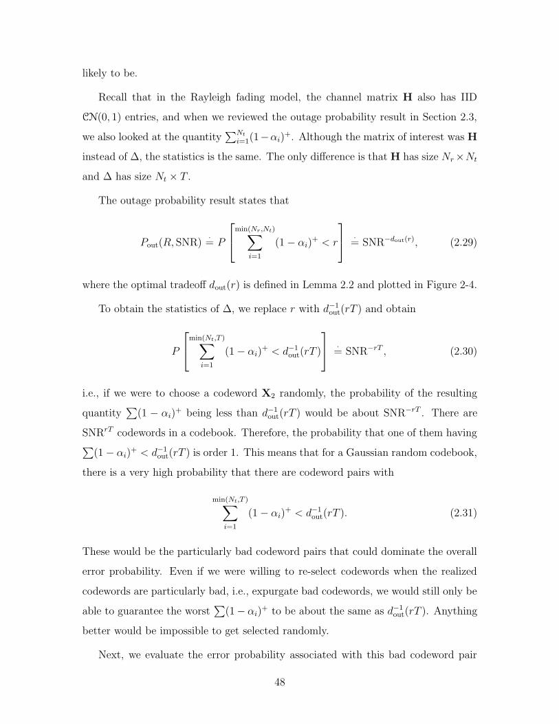
2-10 The upper bound on the diversity-multiplexing tradeoff achievable us-
ing Gaussian random codes based on the worst-pair error probability,
d(r) < 2d−1out(rT ). Short codes with T ≤ 2 are sub-optimal due to the
worst-pair being particularly bad. . . . . . . . . . . . . . . . . . . . . 49
3-1 Comparison of decision boundaries for various detection methods. . . 55
3-2 Using lattice reduction in conjunction with traditional detectors. . . . 57
3-3 Number of iterations needed to find the optimal reduced basis. b1 is
fixed at [1 0]T, each entry of b2 ranges from 0 to 1 in 0.01 increments. 63
3-4 Comparison of the decision regions for MLD and LR-ICD. Minimum
distances to the decision boundaries are also compared. . . . . . . . 65
3-5 Distribution of number of iterations needed for 2×2 lattice reduction. 68
3-6 Symbol error rate curves for various detection methods in the 2 × 2
complex case. The constellation used is 16-QAM. . . . . . . . . . . . 69
3-7 Comparisons of the cumulative density of d2min. . . . . . . . . . . . . . 70
3-8 As constellation size grows, the gap between the symbol error rates
of MLD and LR-BLAST diminishes. The noise level is such that the
SNR is 25 dB for the 16-QAM constellation. . . . . . . . . . . . . . . 71
3-9 Uncoded system with LR-BLAST decoder. The maximum slope reached
is 2. The horizontal spacings between the curves are 6 dB. . . . . . . 72
3-10 When the transmitter knows the channel, it can pre-compensate for
the distortion by transmitting H−1x, so that the received constellation
is the original one. . . . . . . . . . . . . . . . . . . . . . . . . . . . . 73
3-11 At the transmitter, all points that are congruent modulo the constella-
tion region, which form a lattice, are use to represent the same message.
Points labeled “” represent the same message as the point labeled
“+”. At the receiver, any “” can be mapped back to “+” via modulo
operations. . . . . . . . . . . . . . . . . . . . . . . . . . . . . . . . . 74
12

3-12 Treat the original transmitted constellation region, H−1x, as a unit
cell of a lattice. Power reduction can be achieved by using a more
square unit cell corresponding to a different basis as the transmitted
constellation region. Regions shaded in the same way and labeled using
the same number are congruent to each other and represent the same
set of messages. . . . . . . . . . . . . . . . . . . . . . . . . . . . . . . 75
3-13 Empirical distribution of number of iterations needed for n× n (real)
lattice reduction using the LLL algorithm for the cases of n = 2, 4, 6, 8
dimensions. . . . . . . . . . . . . . . . . . . . . . . . . . . . . . . . . 81
3-14 Empirical cumulative distribution, indicating probability of needing x
iterations or more. . . . . . . . . . . . . . . . . . . . . . . . . . . . . 81
3-15 Performance of LR-BLAST detectors using the LLL algorithm, com-
pared to that of the ML detector, for n = 2, 4, 6, 8 dimensional cases.
The ratio dLR−BLASTmin /dMLmin indicates how far LR-BLAST is away from
optimal. . . . . . . . . . . . . . . . . . . . . . . . . . . . . . . . . . . 83
3-16 Performance of LR-ICD detectors using the LLL algorithm, compared
to that of the ML detector, for n = 2, 4, 6, 8 dimensional cases. . . . . 83
4-1 Diversity-multiplexing tradeoff achieved by orthogonal space-time block
code, compared with the optimal tradeoff and that of the expurgated
Gaussian random code, for the case Nt = Nr = T = 2. . . . . . . . . . 88
4-2 Error rate curves of OSTBC (dark) and outage probability curves
(light) for various rates. We see that the maximum diversity of four is
achieved, but there is a loss of multiplexing gain. . . . . . . . . . . . 90
4-3 Rotate (s11, s22) to obtain (x11, x22), so that each non-zero information
symbol pair (s11, s22) leads to both non-zero x11 and non-zero x22 and
effectively appear in both rows and columns of the codeword matrix X. 91
4-4 Maximize the minimum |2 det (X)| as a function of 2θ1 and 2θ2 for the
case where sij each takes the value of 0 and 1. . . . . . . . . . . . . . 93
13
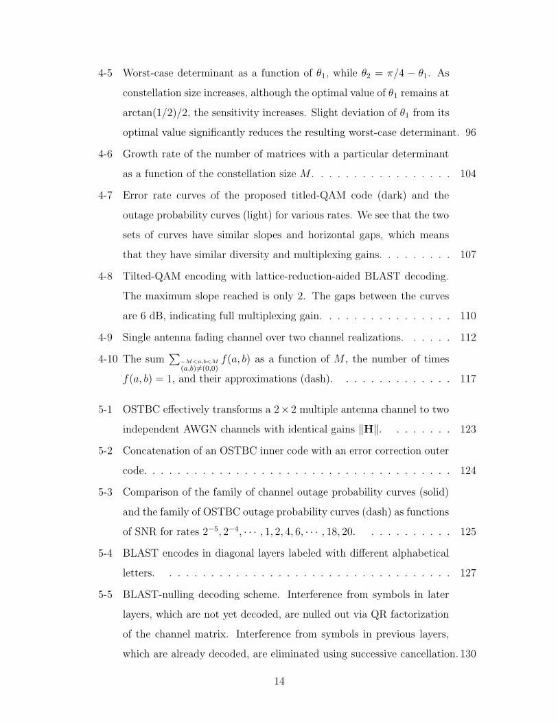
4-5 Worst-case determinant as a function of θ1, while θ2 = π/4 − θ1. As
constellation size increases, although the optimal value of θ1 remains at
arctan(1/2)/2, the sensitivity increases. Slight deviation of θ1 from its
optimal value significantly reduces the resulting worst-case determinant. 96
4-6 Growth rate of the number of matrices with a particular determinant
as a function of the constellation size M . . . . . . . . . . . . . . . . . 104
4-7 Error rate curves of the proposed titled-QAM code (dark) and the
outage probability curves (light) for various rates. We see that the two
sets of curves have similar slopes and horizontal gaps, which means
that they have similar diversity and multiplexing gains. . . . . . . . . 107
4-8 Tilted-QAM encoding with lattice-reduction-aided BLAST decoding.
The maximum slope reached is only 2. The gaps between the curves
are 6 dB, indicating full multiplexing gain. . . . . . . . . . . . . . . . 110
4-9 Single antenna fading channel over two channel realizations. . . . . . 112
4-10 The sum∑
−M<a,b<M
(a,b)6=(0,0)f(a, b) as a function of M , the number of times
f(a, b) = 1, and their approximations (dash). . . . . . . . . . . . . . 117
5-1 OSTBC effectively transforms a 2× 2 multiple antenna channel to two
independent AWGN channels with identical gains ‖H‖. . . . . . . . 123
5-2 Concatenation of an OSTBC inner code with an error correction outer
code. . . . . . . . . . . . . . . . . . . . . . . . . . . . . . . . . . . . . 124
5-3 Comparison of the family of channel outage probability curves (solid)
and the family of OSTBC outage probability curves (dash) as functions
of SNR for rates 2−5, 2−4, · · · , 1, 2, 4, 6, · · · , 18, 20. . . . . . . . . . . 125
5-4 BLAST encodes in diagonal layers labeled with different alphabetical
letters. . . . . . . . . . . . . . . . . . . . . . . . . . . . . . . . . . . 127
5-5 BLAST-nulling decoding scheme. Interference from symbols in later
layers, which are not yet decoded, are nulled out via QR factorization
of the channel matrix. Interference from symbols in previous layers,
which are already decoded, are eliminated using successive cancellation. 130
14
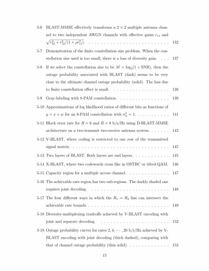
5-6 BLAST-MMSE effectively transforms a 2 × 2 multiple antenna chan-
nel to two independent AWGN channels with effective gains r11 and√r222 + r212/(1 + ρr211). . . . . . . . . . . . . . . . . . . . . . . . . . . 132
5-7 Demonstration of the finite constellation size problem. When the con-
stellation size used is too small, there is a loss of diversity gain. . . . 137
5-8 If we select the constellation size to be M = log2(1 + SNR), then the
outage probability associated with BLAST (dash) seems to be very
close to the ultimate channel outage probability (solid). The loss due
to finite constellation effect is small. . . . . . . . . . . . . . . . . . . 138
5-9 Gray-labeling with 8-PAM constellation. . . . . . . . . . . . . . . . . 139
5-10 Approximations of log likelihood ratios of different bits as functions of
y = x+ w for an 8-PAM constellation with σ2w = 1. . . . . . . . . . . 141
5-11 Block error rate for R = 6 and R = 8 b/s/Hz using D-BLAST-MMSE
architecture on a two-transmit two-receive antenna system. . . . . . . 142
5-12 V-BLAST, where coding is restricted to one row of the transmitted
signal matrix. . . . . . . . . . . . . . . . . . . . . . . . . . . . . . . . 145
5-13 Two layers of BLAST. Both layers are end layers. . . . . . . . . . . . 145
5-14 X-BLAST, where two codewords cross like in OSTBC or tilted-QAM. 146
5-15 Capacity region for a multiple access channel. . . . . . . . . . . . . . 147
5-16 The achievable rate region has two sub-regions. The darkly shaded one
requires joint decoding. . . . . . . . . . . . . . . . . . . . . . . . . . 148
5-17 The four different ways in which the R1 = R2 line can intersect the
achievable rate bounds. . . . . . . . . . . . . . . . . . . . . . . . . . . 149
5-18 Diversity-multiplexing tradeoffs achieved by V-BLAST encoding with
joint and separate decoding. . . . . . . . . . . . . . . . . . . . . . . 152
5-19 Outage probability curves for rates 2, 4, · · · , 20 b/s/Hz achieved by V-
BLAST encoding with joint decoding (thick dashed), comparing with
that of channel outage probability (thin solid). . . . . . . . . . . . . . 153
15
5-20 Outage probability curves for rates 2, 4, · · · , 20 b/s/Hz achieved by
V-BLAST encoding with more practical separate decoding based on
successive cancellation (thick dashed), comparing with that of channel
outage probability (thin solid). . . . . . . . . . . . . . . . . . . . . . . 153
5-21 Diversity-multiplexing tradeoffs achieved by two-layer-D-BLAST en-
coding with joint and separate decoding. . . . . . . . . . . . . . . . 156
5-22 Outage probability curves for rates 2, 4, · · · , 20 b/s/Hz achieved by
two-layer-D-BLAST encoding with joint decoding (thick dashed), com-
paring with that of channel outage probability (thin solid). . . . . . . 158
5-23 Outage probability curves for rates 2, 4, · · · , 20 b/s/Hz achieved by
two-layer-D-BLAST encoding with more practical separate decoding
(thick dashed), comparing with that of channel outage probability (thin
solid). . . . . . . . . . . . . . . . . . . . . . . . . . . . . . . . . . . . 158
5-24 Diversity-multiplexing tradeoffs achieved by X-BLAST encoding with
joint and separate decoding. . . . . . . . . . . . . . . . . . . . . . . 159
5-25 Outage probability curves for rates 2, 4, · · · , 20 b/s/Hz achieved by X-
BLAST encoding with more practical separate decoding (thick dashed),
comparing with doing joint decoding, which is also the channel outage
probability (thin solid). . . . . . . . . . . . . . . . . . . . . . . . . . . 160
5-26 Gaps to capacity as a function of rate at Pout = 10−3 for various sys-
tems. . . . . . . . . . . . . . . . . . . . . . . . . . . . . . . . . . . . 161
5-27 Diversity-multiplexing tradeoff curves achieved by variations of BLAST
in block form and OSTBC. . . . . . . . . . . . . . . . . . . . . . . . . 162
5-28 Concatenation of a tilted-QAM inner code with a Reed-Solomon outer
code. . . . . . . . . . . . . . . . . . . . . . . . . . . . . . . . . . . . . 164
5-29 Block error rate curves for 16-QAM, 64-QAM, and 256-QAM cases.
As we gradually reduce the data rate by 1 b/s/Hz, the block error rate
lowers due to stronger coding. However, the gain diminishes. . . . . . 166
16
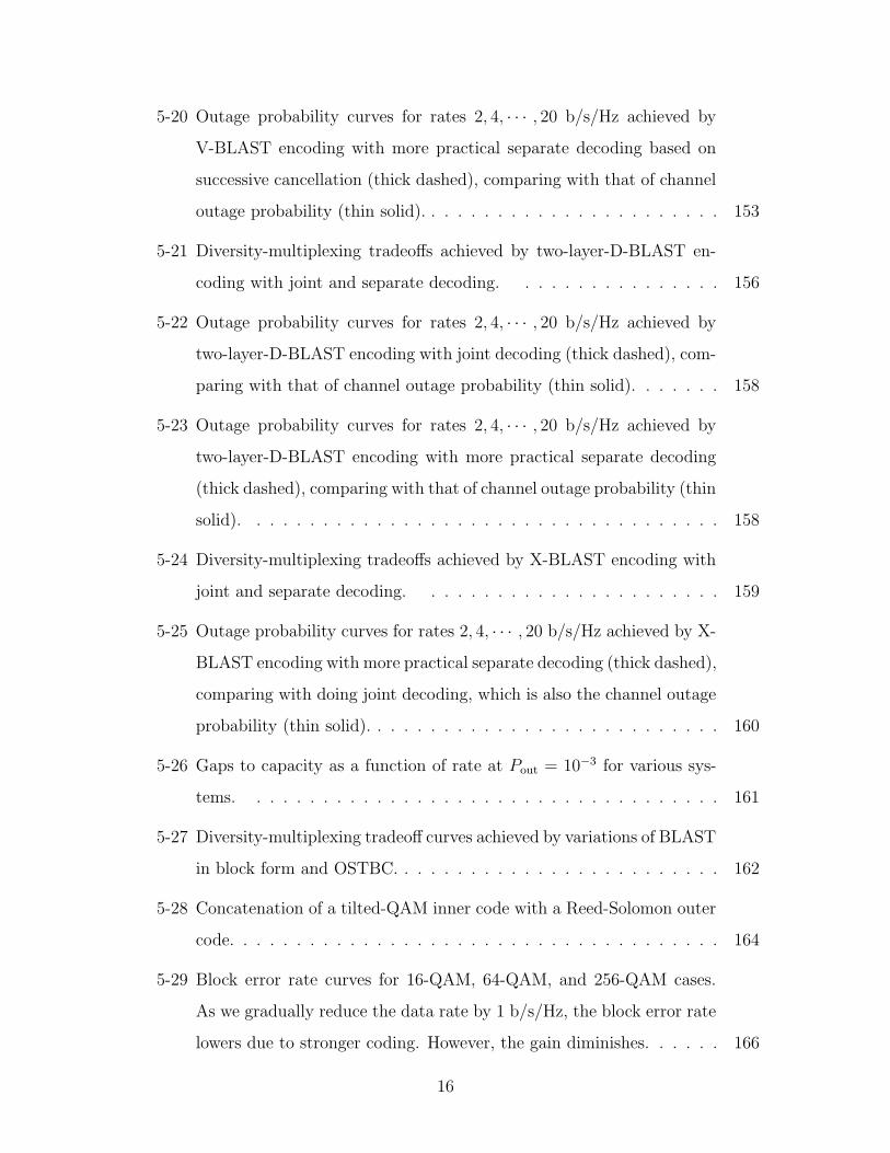
5-30 Block error rate curves for 16-QAM, 64-QAM, and 256-QAM cases
with 1 b/s/Hz rate reduction using RS coding. The unmarked curves
are the corresponding channel outage probability curves. . . . . . . . 167
5-31 Concatenation of a tilted-QAM inner code with an LDPC outer code
with a two component iterative soft-decision decoder. . . . . . . . . 168
5-32 Passing of bit-wise LLR scores between an LDPC decoder and a lattice-
aware detector unit consisting of a lattice detector and an MMSE de-
tector. . . . . . . . . . . . . . . . . . . . . . . . . . . . . . . . . . . . 170
5-33 Block error rates achieved by tilted-QAM-LDPC concatenated systems
(thick solid), compared with D-BLAST-MMSE (dashed), and the ulti-
mate outage probability limit (thin solid), at R = 6 and R = 8 b/s/Hz,
using two-transmit two-receive antenna systems. . . . . . . . . . . . . 173
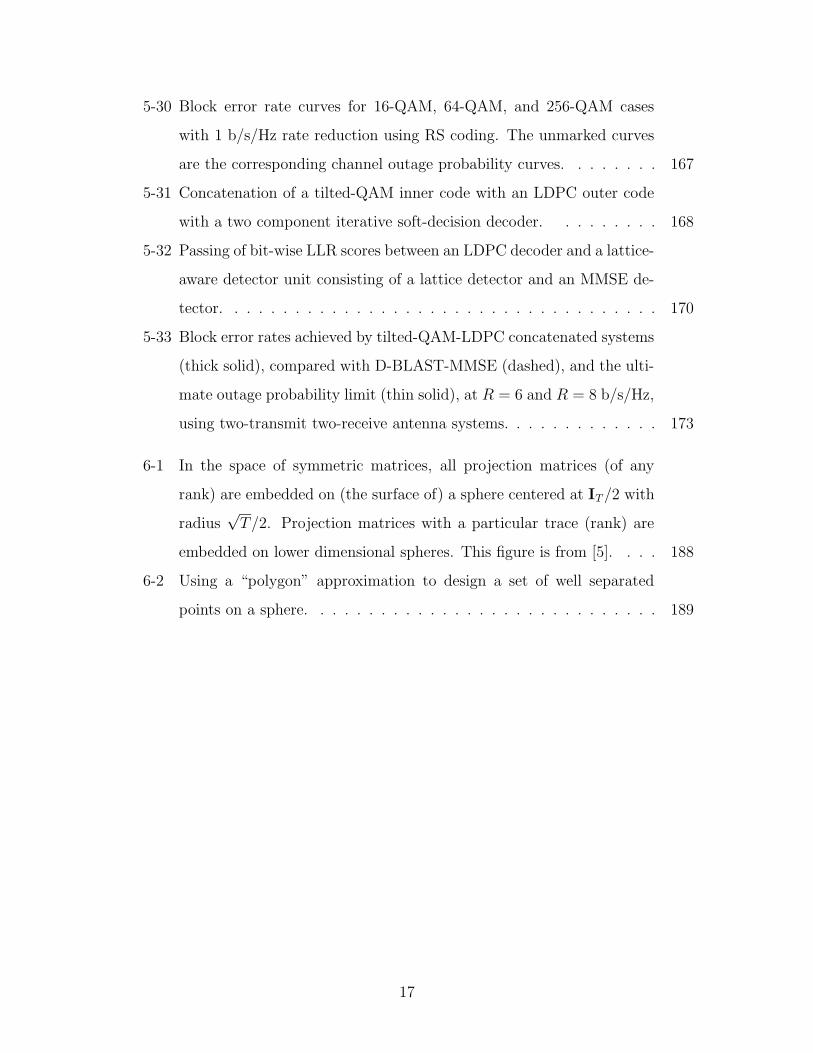
6-1 In the space of symmetric matrices, all projection matrices (of any
rank) are embedded on (the surface of) a sphere centered at IT/2 with
radius√T/2. Projection matrices with a particular trace (rank) are
embedded on lower dimensional spheres. This figure is from [5]. . . . 188
6-2 Using a “polygon” approximation to design a set of well separated
points on a sphere. . . . . . . . . . . . . . . . . . . . . . . . . . . . . 189
17

18
Chapter 1
Introduction
Over the past few years, it has been shown that using multiple antennas can sig-
nificantly increase the capacity and robustness of communication systems in fading
environments. Capacity grows with the number of antennas used. Approximately
twice the amount of information can be communicated using two transmit antennas
and two receive antennas, without spending any extra time, bandwidth, nor power.
In a fading environment, the channel quality may vary due to, for example, movement
of the transmitter or the receiver. In such an environment, using multiple antennas
makes it less likely for the channel to be in a deep enough fade such that the trans-
mitted information can not go through. This is because the multiple links between
the multiple antennas provide us with multiple opportunities and more protection.
Since the benefits of using multiple antennas have been recognized, much work
have been done toward designing coding and decoding schemes to realize these gains
promised by theoretical studies. However, some of the studies focus only on the
robustness gain but do not capitalize on the capacity gain; while others concentrate
on the capacity gain but have less than optimal robustness.
More recently, there are efforts on realizing both capacity and robustness gains
simultaneously. Zheng and Tse [41] established that there is a tradeoff between these
two types of gains, i.e., how fast error probability can decay and how rapidly data rate
can increases with signal to noise ratio (SNR). Furthermore, they analytically evalu-
ated the efficient frontier of this diversity-multiplexing tradeoff for systems with any
19
number of transmit and receive antennas and showed that the frontier is achievable
using sufficiently long Gaussian random codes.
In this thesis, our goal is to design practical multiple antenna systems aiming at
achieving the optimal diversity-multiplexing tradeoff. We design structured linear
signaling and coding schemes at the transmitter with easy implementation, and de-
sign corresponding decoding algorithms at the receiver with moderate computational
complexity. We demonstrate the performance of our designs through both theoretical
analysis and numerical simulations.
1.1 Channel and System Model
hN NN
h
h
h
hh11
22
12 21
1N
x
x y
y
2
N
y1
h2N
hN 1
hN 2
2
1
xN
w
w
w
1
2
t rr
r
t
t
r
t r
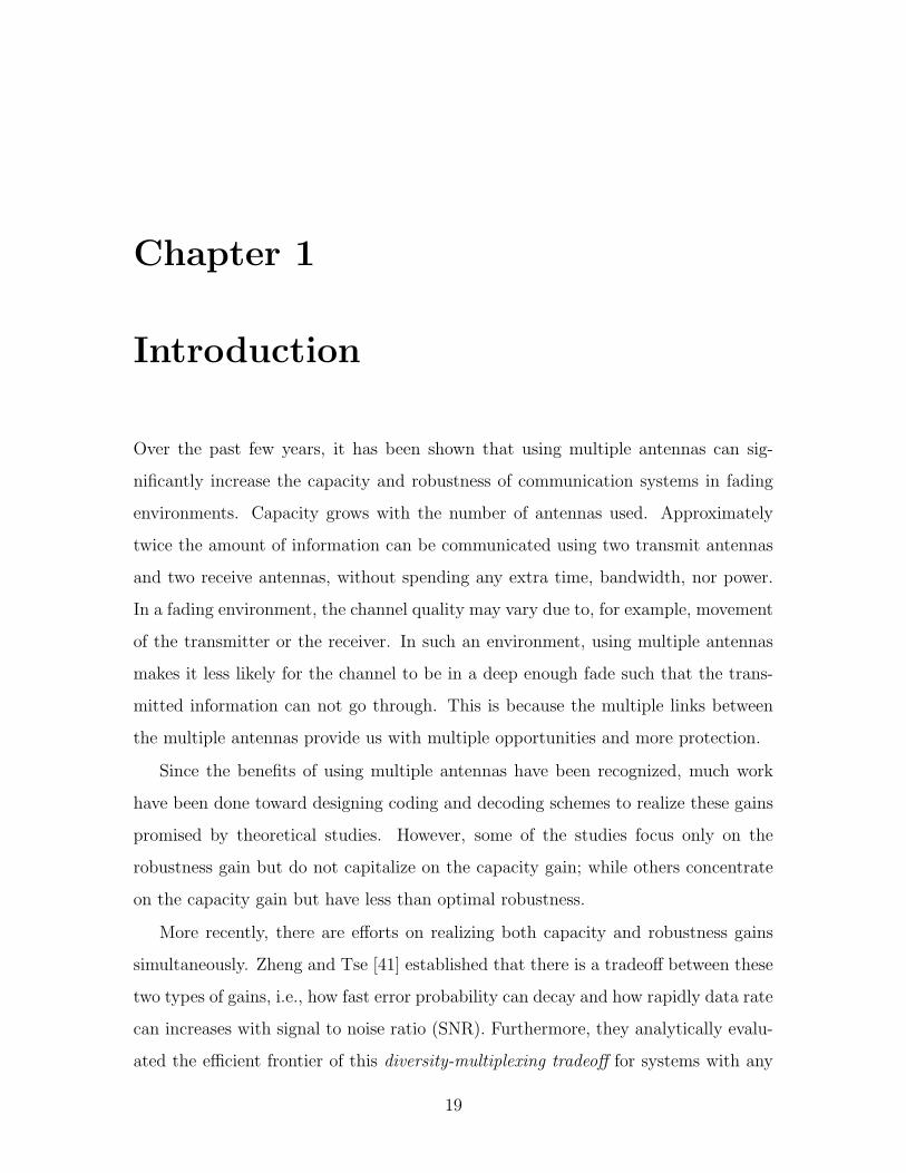
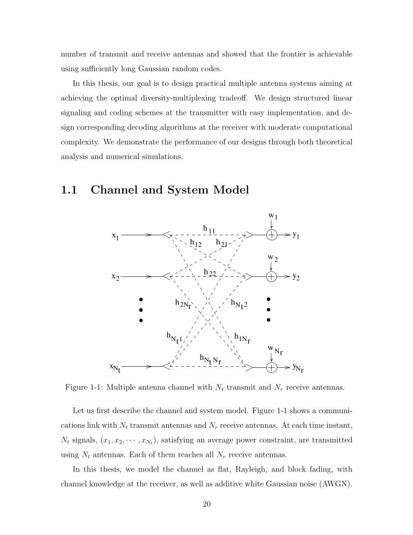
Figure 1-1: Multiple antenna channel with Nt transmit and Nr receive antennas.
Let us first describe the channel and system model. Figure 1-1 shows a communi-
cations link with Nt transmit antennas and Nr receive antennas. At each time instant,
Nt signals, (x1, x2, · · · , xNt), satisfying an average power constraint, are transmitted
using Nt antennas. Each of them reaches all Nr receive antennas.
In this thesis, we model the channel as flat, Rayleigh, and block fading, with
channel knowledge at the receiver, as well as additive white Gaussian noise (AWGN).
20
These models are commonly used in the multiple antenna communications literature
and have been proven useful in practice. We also restrict our attention to the case
where there are at least as many receive antennas as transmit antennas, i.e., Nr ≥ Nt.
• Flat Fading: We model each wireless link between each pair of transmit and
receive antennas as a simple scaling by channel gain hij. This is valid when the
signal bandwidth is narrow enough so that the entire spectrum experiences the
same fading coefficient.
• Rayleigh Fading: We model the statistics of the random channel coefficients,
hij, using the Rayleigh fading model. This means that they are independent
and identically distributed (IID) with zero mean, unit variance, circularly sym-
metric, complex Gaussian density, CN(0, 1). It is worth noting that this model
is often used because it leads to more tractable theoretical analysis, but it is not
entirely accurate. In most environments, the channel coefficients are correlated.
The correlation is less when the antennas are well separated and there are a large
number of scatters in the environment. Given a particular environment, only a
certain number of antennas can be used before the channel coefficients become
too correlated and the channel model breaks down. For example, for indoor
environments, only up to three to eight antennas can be used [27]. Therefore,
practically speaking, we can not indefinitely increase the number of antennas
used and hope to obtain arbitrarily large capacity and robustness gains.
• Block Fading: We model the time varying nature of the channel using block
fading, meaning that the channel stays fixed for a certain period, call the co-
herence time of the channel, and then changes to something independent for
the next block. In reality, channel coefficients changes gradually from one time
instant to the next. However, this is hard to analyze. Therefore, block fading
model is often used for its simplicity.
• Channel Knowledge at Receiver: For most of this thesis, we assume that
perfect channel knowledge is available at the receiver but not at the transmitter,
21
i.e., coherent detection. Practically speaking, the receiver can not know the
channel perfectly. However, if the channel varies slowly, we can assume that the
receiver has sufficient time to get a good estimate of the channel. Again, this
assumption is not entirely accurate but makes our problem easier. In Chapter 6,
we explore the scenario where no channel knowledge is available, which we call
non-coherent detection. This happens when the channel varies too fast and is
difficult to track. We always assume that transmitter does not have knowledge
of the channel, because this requires feedback from the receiver.
• AWGN at Receiver: At each receiver, signals received from all transmit an-
tennas are added together, along with an IID additive white (complex) Gaussian
noise with zero mean and variance per dimension σ2w, i.e., CN(0, 2σ2w).
We also restrict our attention to the case where the code duration, denoted by T ,
is shorter than the coherence time of the channel, so that each codeword experiences
only one channel realization. The system we design can serve as a building block to
build more complex systems where coding happens over multiple channel realizations
through interleaving in either time or frequency or both.
With the above channel models, we can express the multiple antenna channel
(over one channel realization) mathematically as
Y = HX+W, (1.1)
where H is the Nr × Nt, Nr ≥ Nt, multiple antenna channel, X is the Nt × T
transmitted signal matrix,W represents the additive white Gaussian noise, and Y is
the received signal matrix. Written in a matrix form, we have
y11 · · · y1Ty21 · · · y2T...
. . ....
yNr1 · · · yNrT
=
h11 · · · h1Nt
h21 · · · h2Nt
.... . .
...
hNr1 · · · hNrNt
x11 · · · x1Tx21 · · · x2T...
. . ....
xNt1 · · · xNtT
+
w11 · · · w1T
w21 · · · w2T
.... . .
...
wNr1 · · · wNrT
. (1.2)
22
Let the energy constraint on the transmitted signal be such that each dimension of
xij has an average energy of Es. The total transmit SNR over all antennas is thus
SNR = NtEs
σ2w. (1.3)
The per-antenna SNR is
ρ =SNR
Nt
=Es
σ2w. (1.4)
Note that each column of the transmitted signal matrix X corresponds to what is
transmitted at one time by multiple antennas; and each row corresponds to what one
antenna transmits over time. When we perform coding across rows of X, we refer to
it as coding across space. Coding across columns is referred to as coding across time.
When the transmission rate is R b/s/Hz, there are 2RT codeword matrices X to be
designed.
1.2 Thesis Outline
We first review some theoretical background on multiple antenna communications
in Chapter 2. We present the channel capacity formula and define the ultimate
performance limit, the outage probability. We then review the diversity-multiplexing
tradeoff definition and the optimal tradeoff result obtained by Zheng and Tse [41],
and provide some of our own interpretations. Next, we look at what determines
the error probabilities of a given coding scheme, and from which we obtain some
code design rules. We then analyze Gaussian random codes as a benchmark and
see that sufficiently long Gaussian random codes can achieve the optimal diversity
multiplexing tradeoff while shorts ones can not due to particularly bad randomly
selected codeword pairs.
In this thesis, our goal is to design practical multiple antenna systems aiming at
achieving the optimal diversity-multiplexing tradeoff. we focus our research on the
two-transmit two-receive antenna system, which arises frequently in practice, and can
23

lead to important insights on how to build larger systems with more antennas. We
study the design problem in various delay and complexity regimes.
In Chapter 3, we investigated the case of uncoded transmission with zero delay,
i.e., code duration T = 1. We propose low-complexity detectors that can achieve
near maximum likelihood performance by operating traditional detectors in a reduced
lattice basis. We identify the optimal basis to operate in and describe an iterative
algorithm for finding it. Using these improved detectors, the uncoded system achieves
the best diversity-multiplexing tradeoff achievable by any length-one code.
In Chapter 4, we move on to the case of coding with the minimum delay necessary
for achieving the optimal diversity-multiplexing tradeoff. We construct a family of
short structured space-time block codes for the two-transmit two-receive antenna
system. It achieves the optimal diversity-multiplexing tradeoff and has the minimum
delay of two necessary for optimality. It is a modification of the well-known orthogonal
space-time block codes (OSTBC) [1, 34], which uses a smart repetition to achieve
the maximum diversity gain at the expense of multiplexing gain. We use an idea of
rotation, instead of repetition, of cross-diagonal entries of an uncoded transmission to
achieve spreading of information across space and time to obtain maximum diversity
while preserving multiplexing gain. Rotation angles that are optimal in terms of a
determinant criterion and universal for all rates are identified. We refer to this code
construction as the tilted-QAM code.
In Chapter 5, we experiment with further enhancing system performance using
powerful error correction codes (ECC). The goal is to understand how to build practi-
cal systems with good performance. We study several coding systems. We show that
an system based on OSTBC can achieve near optimal performance in the low SNR
regime. We then describe the Bell labs layered space-time (BLAST) architecture and
show that it has the potential to achieve channel capacity but has practical problems.
We also present and analyze several variations of the BLAST. Finally, we explore
the possibility of combining hard and soft decision error correction coding with the
tilted-QAM code.
In Chapter 6, we explore the case where channel knowledge is available at neither
24

the transmitter nor the receiver. We first review some existing theoretical results
on non-coherent multiple antenna communications, and then discuss the problem of
signal design. We present evidence that the channel training approach could lead to
good diversity-multiplexing tradeoff.
In Chapter 7, we summarize the contributions of this thesis and discuss future
research directions.
25

26
Chapter 2
Theoretical Background
In this chapter, we first review the channel capacity formulation and the concept
of outage probability, which sets the ultimate performance limit. In section 2.2,
we illustrate the capacity and robustness gains that can be potentially obtained us-
ing multiple antennas. In section 2.3, we review the diversity-multiplexing tradeoff
framework and provide additional intuition. In section 2.4, we derive error probabil-
ity expressions for evaluating coding schemes and obtain criteria for good codes. In
section 2.5, we use the formulation from section 2.4 to examine the performance of
Gaussian random codes of different lengths. We explain why short Gaussian random
codes can not achieve the optimal diversity-multiplexing tradeoff.
2.1 Channel Capacity and Outage Probability
Given a particular channel realization H, the theoretical limit of the amount of data
we can transmit through the channel reliably, i.e., with arbitrarily low error rate, is
the channel capacity [36],
Cchannel(H, ρ) = log2(det(INr+ ρHH†)) b/s/Hz, (2.1)
where ρ = SNR/Nt is the average transmit SNR per antenna and det(·) denotes thedeterminant function. This data rate is achievable using infinitely long codes with
27
unlimited complexity. We note that the input distribution used is CN(0, ρ). Since,
the transmitter has no knowledge of the channel, this distribution is a reasonable
default choice. If the channel were known, it would be possible to choose a better
input distribution.
Another important concept is outage. In our system model, coding is performed
over one channel realization, and since the channel is a random matrix, the realized
channel capacity is a random variable. Since the transmitter has no knowledge of the
channel, it can not adjust the data rate according to the realized channel and must
transmit at a fixed rate R b/s/Hz. Therefore, when the realized channel capacity is
below R, the receiver can not decode even with powerful codes. This is the outage
event, and the outage probability is
Pout(R, ρ) = P [C(H, ρ) < R]. (2.2)
This is the ultimate performance limit when coding is done over only one channel
realization.
Achieving the outage probability requires using infinitely long and complex codes.
In practice, long codes leads to large delay and high complexity requires expensive
hardware. Therefore, they are usually not satisfied in practice, and we must content
with finite delay and moderate complexity coding schemes. The capacity formulas
can be used as performance limits and help us evaluate practical systems.
2.2 Visualizing Rate and Robustness Gains
Next, let us use the capacity and outage probability formulation to gain some insight
into how capacity and robustness gains can be obtained using multiple antennas.
In the single antenna case, which is simply the AWGN channel (y = hx+w), the
well-known channel capacity, originally derived by Shannon, is
Cchannel(H, ρ) = log2(ρ|h|2 + 1
). (2.3)
28
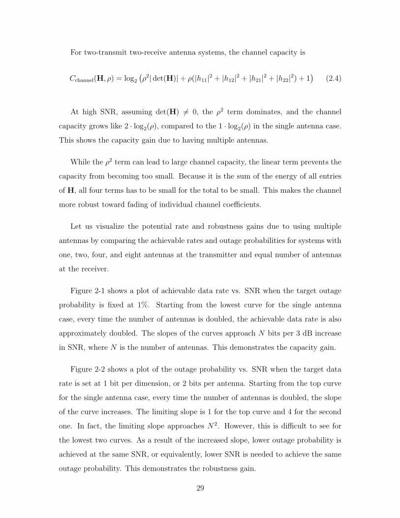
For two-transmit two-receive antenna systems, the channel capacity is
Cchannel(H, ρ) = log2(ρ2| det(H)|+ ρ(|h11|2 + |h12|2 + |h21|2 + |h22|2) + 1
)(2.4)
At high SNR, assuming det(H) 6= 0, the ρ2 term dominates, and the channel
capacity grows like 2 · log2(ρ), compared to the 1 · log2(ρ) in the single antenna case.
This shows the capacity gain due to having multiple antennas.
While the ρ2 term can lead to large channel capacity, the linear term prevents the
capacity from becoming too small. Because it is the sum of the energy of all entries
of H, all four terms has to be small for the total to be small. This makes the channel
more robust toward fading of individual channel coefficients.
Let us visualize the potential rate and robustness gains due to using multiple
antennas by comparing the achievable rates and outage probabilities for systems with
one, two, four, and eight antennas at the transmitter and equal number of antennas
at the receiver.
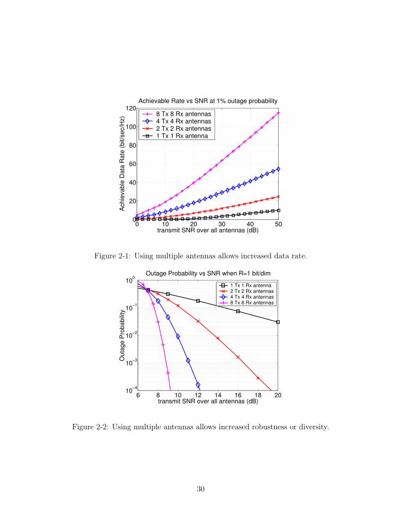
Figure 2-1 shows a plot of achievable data rate vs. SNR when the target outage
probability is fixed at 1%. Starting from the lowest curve for the single antenna
case, every time the number of antennas is doubled, the achievable data rate is also
approximately doubled. The slopes of the curves approach N bits per 3 dB increase
in SNR, where N is the number of antennas. This demonstrates the capacity gain.
Figure 2-2 shows a plot of the outage probability vs. SNR when the target data
rate is set at 1 bit per dimension, or 2 bits per antenna. Starting from the top curve
for the single antenna case, every time the number of antennas is doubled, the slope
of the curve increases. The limiting slope is 1 for the top curve and 4 for the second
one. In fact, the limiting slope approaches N 2. However, this is difficult to see for
the lowest two curves. As a result of the increased slope, lower outage probability is
achieved at the same SNR, or equivalently, lower SNR is needed to achieve the same
outage probability. This demonstrates the robustness gain.
29
0 10 20 30 40 500
20
40
60
80
100
120
transmit SNR over all antennas (dB)
Ach
ieva
ble
Dat
a R
ate
(bit/
sec/
Hz)
Achievable Rate vs SNR at 1% outage probability
8 Tx 8 Rx antennas4 Tx 4 Rx antennas2 Tx 2 Rx antennas1 Tx 1 Rx antenna
Figure 2-1: Using multiple antennas allows increased data rate.
6 8 10 12 14 16 18 2010−4
10−3
10−2
10−1
100
transmit SNR over all antennas (dB)
Out
age
Pro
babi
lity
Outage Probability vs SNR when R=1 bit/dim
1 Tx 1 Rx antenna2 Tx 2 Rx antennas4 Tx 4 Rx antennas8 Tx 8 Rx antennas
Figure 2-2: Using multiple antennas allows increased robustness or diversity.
30
2.3 Diversity-Multiplexing Tradeoff
Using multiple antennas can provide us both data rate gain as well as robustness gain
toward channel fading, as we demonstrated in the last section. However, a tradeoff
exists between these two types of gains; getting more of one kind requires sacrifice of
the other. This tradeoff was defined and studied by Zheng and Tse in [41].
In this section, we first introduce the definition of diversity and multiplexing gains,
and then review the main results on the optimal tradeoff achievable. Next, we focus on
the two-transmit two-receive antenna case, examine the tradeoff analytically, as well
as visualize it by plotting families of outage probability curves. Finally, we comment
on local diversity-multiplexing tradeoff.
2.3.1 Definitions
For a given SNR, let R(SNR) be the transmission rate and Pe(SNR) be the error
probability at that rate and SNR. Diversity gain (d) and multiplexing gain (r) are
defined as
d = − lim supSNR→∞
logPe(SNR)
log SNR, (2.5)
and
r = limSNR→∞
R(SNR)
log2 SNR. (2.6)
Intuitively, multiplexing gain is about how fast rate increases with SNR, and
diversity gain describes how fast error probability decays with SNR. If we let rate grow
rapidly with SNR, error probability would not decay very fast. This is a fundamental
tradeoff. This diversity-multiplexing tradeoff can be used to evaluate and compare
coding schemes.
For simplicity, we use some special notations defined in [41]. We use·= to denote
31
exponential equality, i.e., f(x)·= xb denotes
lim supx→∞
log f(x)
log x= b.
With this notation, diversity gain can also be written as
Pe(SNR)·= SNR−d. (2.7)
The notations·≥ and
·≤ are defined similarly.
2.3.2 Optimal Tradeoff Results
Before looking at any particular system, let us consider the diversity-multiplexing
tradeoff associated with the outage probability, i.e., replacing the error probability
Pe(SNR) in (2.5) with the outage probability Pout(SNR). When the channel is in
outage, there would be a high error probability no matter what coding scheme is used.
Therefore, the diversity-multiplexing tradeoff associated with the outage probability,
denoted by dout(r), is an upper bound of the optimal tradeoff achievable by any
system. It was shown in [41] that the tradeoff dout(r) is in fact achievable using
sufficiently long Gaussian random codes.
For a system with Nt transmit antennas and Nr receive antennas, Zheng and Tse
evaluated dout(r) in [41] and their main result is stated in the following lemma :
Lemma 2.1 The optimal tradeoff curve dout(r) is given by the piece-wise linear func-
tion connecting the points (k, dout(k)), k = 0, · · · , K where K = min(Nt, Nr), and
dout(k) = (Nt − k)(Nr − k). (2.8)
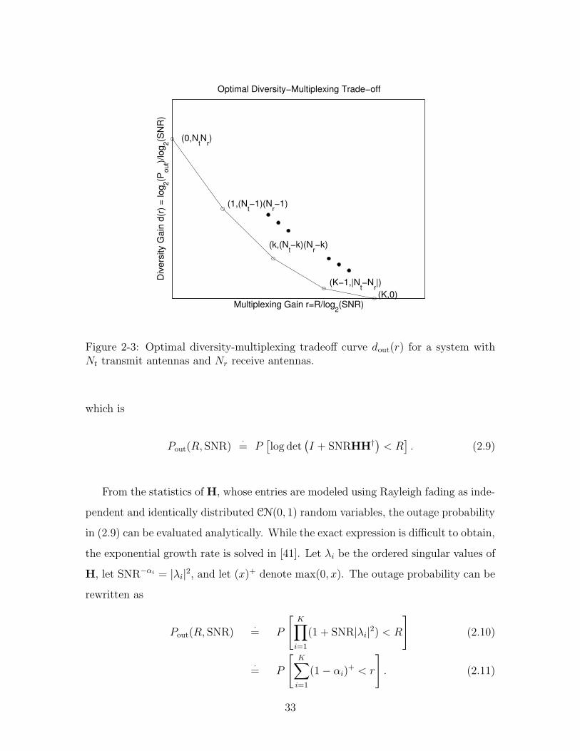
The function dout(r) is plotted in Figure 2-3 for general values of Nt and Nr.
The tradeoff curve dout(r) can be evaluated from the outage probability Pout(R, SNR),
32
Multiplexing Gain r=R/log2(SNR)
Div
ersi
ty G
ain
d(r)
= lo
g 2(Pou
t)/log
2(SN
R)
Optimal Diversity−Multiplexing Trade−off
(0,NtN
r)
(1,(Nt−1)(N
r−1)
(k,(Nt−k)(N
r−k)
(K−1,|Nt−N
r|)(K,0)
Figure 2-3: Optimal diversity-multiplexing tradeoff curve dout(r) for a system withNt transmit antennas and Nr receive antennas.
which is
Pout(R, SNR)·= P
[log det
(I + SNRHH†
)< R
]. (2.9)
From the statistics of H, whose entries are modeled using Rayleigh fading as inde-
pendent and identically distributed CN(0, 1) random variables, the outage probability
in (2.9) can be evaluated analytically. While the exact expression is difficult to obtain,
the exponential growth rate is solved in [41]. Let λi be the ordered singular values of
H, let SNR−αi = |λi|2, and let (x)+ denote max(0, x). The outage probability can be
rewritten as
Pout(R, SNR)·= P
[K∏
i=1
(1 + SNR|λi|2) < R
](2.10)
·= P
[K∑
i=1
(1− αi)+ < r
]. (2.11)
33
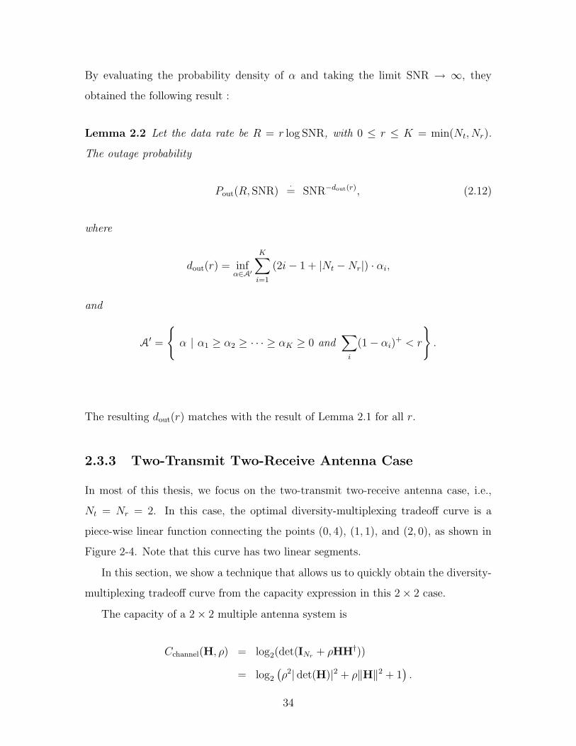
By evaluating the probability density of α and taking the limit SNR → ∞, they
obtained the following result :
Lemma 2.2 Let the data rate be R = r log SNR, with 0 ≤ r ≤ K = min(Nt, Nr).
The outage probability
Pout(R, SNR)·= SNR−dout(r), (2.12)
where
dout(r) = infα∈A′
K∑
i=1
(2i− 1 + |Nt −Nr|) · αi,
and
A′ =
α | α1 ≥ α2 ≥ · · · ≥ αK ≥ 0 and
∑
i
(1− αi)+ < r
.
The resulting dout(r) matches with the result of Lemma 2.1 for all r.
2.3.3 Two-Transmit Two-Receive Antenna Case
In most of this thesis, we focus on the two-transmit two-receive antenna case, i.e.,
Nt = Nr = 2. In this case, the optimal diversity-multiplexing tradeoff curve is a
piece-wise linear function connecting the points (0, 4), (1, 1), and (2, 0), as shown in
Figure 2-4. Note that this curve has two linear segments.
In this section, we show a technique that allows us to quickly obtain the diversity-
multiplexing tradeoff curve from the capacity expression in this 2× 2 case.
The capacity of a 2× 2 multiple antenna system is
Cchannel(H, ρ) = log2(det(INr+ ρHH†))
= log2(ρ2| det(H)|2 + ρ‖H‖2 + 1
).
34

0 1 4/3 2 0
1
2
4
Multiplexing Gain r=R/log2(SNR)
Div
ersi
ty G
ain
d out(r
)
Optimal Tradeoff for N t=N
r=2 case
Figure 2-4: Optimal diversity-multiplexing tradeoff curve dout(r) for the two-transmittwo-receive antenna case.
Performing a QR factorization of H = QR, where R =
r11 r12
0 r22
, the above expres-
sion can be rewritten as
Cchannel(H, ρ) = log2(ρ2r211r
222 + ρ(r211 + |r12|2 + r222) + 1
). (2.13)
The term r211 is the energy of the first column of H, so it is the sum of the squares
of four independent Gaussian random variables. Thus, it is a chi-squared random
variable of order 4. Similarly, |r12|2 and r222 are the energy of the second column of
H that are along and perpendicular to the direction of the first column. Therefore,
they are chi-squared random variables of order 2. Note that for a chi-squared random
variable χ of order k, P [χ < α]·= αk/2, for α < 1.
Using 2R·= ρr, the outage probability can be written as
Pout·= P [ρ2r211r
222 + ρ(r211 + |r12|2 + r222) + 1 < ρr]. (2.14)
For 1 ≤ r ≤ 2, the first order and the constant terms are insignificant compared
35
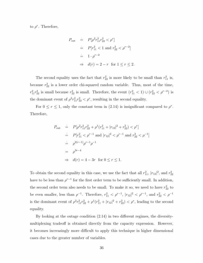
to ρr. Therefore,
Pout·= P [ρ2r211r
222 < ρr]
·= P [r211 < 1 and r222 < ρr−2]
·= 1 · ρr−2
⇒ d(r) = 2− r for 1 ≤ r ≤ 2.
The second equality uses the fact that r222 is more likely to be small than r211 is,
because r222 is a lower order chi-squared random variable. Thus, most of the time,
r211r222 is small because r222 is small. Therefore, the event (r211 < 1) ∪ (r222 < ρr−2) is
the dominant event of ρ2r211r222 < ρr, resulting in the second equality.
For 0 ≤ r ≤ 1, only the constant term in (2.14) is insignificant compared to ρr.
Therefore,
Pout·= P [ρ2r211r
222 + ρ1(r211 + |r12|2 + r222) < ρr]
·= P [r211 < ρr−1 and |r12|2 < ρr−1 and r222 < ρ−1]
·= ρ2(r−1)ρr−1ρ−1
= ρ3r−4
⇒ d(r) = 4− 3r for 0 ≤ r ≤ 1.
To obtain the second equality in this case, we use the fact that all r211, |r12|2, and r222have to be less than ρr−1 for the first order term to be sufficiently small. In addition,
the second order term also needs to be small. To make it so, we need to have r222 to
be even smaller, less than ρ−1. Therefore, r211 < ρr−1, |r12|2 < ρr−1, and r222 < ρ−1
is the dominant event of ρ2r211r222 + ρ1(r211 + |r12|2 + r222) < ρr, leading to the second
equality.
By looking at the outage condition (2.14) in two different regimes, the diversity-
multiplexing tradeoff is obtained directly from the capacity expression. However,
it becomes increasingly more difficult to apply this technique in higher dimensional
cases due to the greater number of variables.
36
2.3.4 Visualizing The Tradeoff
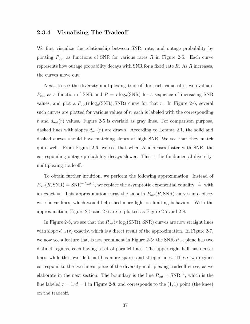
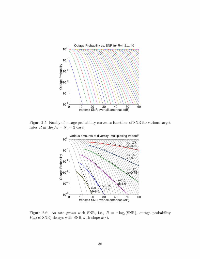
We first visualize the relationship between SNR, rate, and outage probability by
plotting Pout as functions of SNR for various rates R in Figure 2-5. Each curve
represents how outage probability decays with SNR for a fixed rate R. As R increases,
the curves move out.
Next, to see the diversity-multiplexing tradeoff for each value of r, we evaluate
Pout as a function of SNR and R = r log2(SNR) for a sequence of increasing SNR
values, and plot a Pout(r log2(SNR), SNR) curve for that r. In Figure 2-6, several
such curves are plotted for various values of r; each is labeled with the corresponding
r and dout(r) values. Figure 2-5 is overlaid as gray lines. For comparison purpose,
dashed lines with slopes dout(r) are drawn. According to Lemma 2.1, the solid and
dashed curves should have matching slopes at high SNR. We see that they match
quite well. From Figure 2-6, we see that when R increases faster with SNR, the
corresponding outage probability decays slower. This is the fundamental diversity-
multiplexing tradeoff.
To obtain further intuition, we perform the following approximation. Instead of
Pout(R, SNR)·= SNR−dout(r), we replace the asymptotic exponential equality
·= with
an exact =. This approximation turns the smooth Pout(R, SNR) curves into piece-
wise linear lines, which would help shed more light on limiting behaviors. With the
approximation, Figure 2-5 and 2-6 are re-plotted as Figure 2-7 and 2-8.
In Figure 2-8, we see that the Pout(r log2(SNR), SNR) curves are now straight lines
with slope dout(r) exactly, which is a direct result of the approximation. In Figure 2-7,
we now see a feature that is not prominent in Figure 2-5: the SNR-Pout plane has two
distinct regions, each having a set of parallel lines. The upper-right half has denser
lines, while the lower-left half has more sparse and steeper lines. These two regions
correspond to the two linear piece of the diversity-multiplexing tradeoff curve, as we
elaborate in the next section. The boundary is the line Pout = SNR−1, which is the
line labeled r = 1, d = 1 in Figure 2-8, and corresponds to the (1, 1) point (the knee)
on the tradeoff.
37
0 10 20 30 40 50 6010−5
10−4
10−3
10−2
10−1
100
transmit SNR over all antennas (dB)
Out
age
Pro
babi
lity
Outage Probability vs. SNR for R=1,2,...,40
Figure 2-5: Family of outage probability curves as functions of SNR for various targetrates R in the Nt = Nr = 2 case.
0 10 20 30 40 50 6010−5
10−4
10−3
10−2
10−1
100
transmit SNR over all antennas (dB)
Out
age
Pro
babi
lity
various amounts of diversity−multiplexing tradeoff
r=1.75d=0.25
r=1.5d=0.5
r=1.25d=0.75
r=1.0d=1.0
r=0.75d=1.75r=0.5
d=2.5
Figure 2-6: As rate grows with SNR, i.e., R = r log2(SNR), outage probabilityPout(R, SNR) decays with SNR with slope d(r).
38
0 10 20 30 40 50 6010−5
10−4
10−3
10−2
10−1
100
transmit SNR over all antennas (dB)
Out
age
Pro
babi
lity
Outage Probability vs. SNR for R=1,2,...,40
Figure 2-7: Linearized approximation of Figure 2-5, which clearly shows two regionsof the Pout-SNR space with different slopes of curves and horizontal spacings betweencurves.
0 10 20 30 40 50 6010−5
10−4
10−3
10−2
10−1
100
r=1.75d=0.25
r=1.5d=0.5
r=1.25d=0.75
r=1.0d=1.0r=0.75
d=1.75r=0.5d=2.5
transmit SNR over all antennas (dB)
Out
age
Pro
babi
lity
various amounts of diversity−multiplexing tradeoff
Figure 2-8: Linearized approximation of Figure 2-6.
39
2.3.5 Local Diversity-Multiplexing Tradeoff
The slopes and gaps between the curves in Figure 2-7 lead to a concept called local
diversity-multiplexing tradeoff, which is different from the global scale tradeoff we
have defined. Let us suppose that we are operating at a certain (R, SNR, Pout) point.
If we were given an increment of SNR (in dB), the local tradeoff characterizes the
relationship between the incremental increase in rate and the reduction of Pout.
Let us now visualize this local tradeoff by looking at Figure 2-7. When the oper-
ating point has Pout > SNR−1, we are in the upper-right region, which has a set of
parallel lines with slopes 2 and horizontal spacings of 1.5 dB between lines with rate
differential 1 b/s/Hz. This means that if we spend all the extra SNR on increasing
rate and keep Pout constant, we can get 2 extra b/s/Hz for every additional 3 dB in
SNR. If we spend all the extra SNR on the reduction of Pout and keep rate constant,
we can get 2 orders of magnitude reduction for every additional 10 dB in SNR. We
can also get any linear combination of the two extremes because the lines are paral-
lel. Therefore, the local tradeoff is a straight line connecting (r, d) = (0, 2) and (2, 0),
which is the lower piece of the global tradeoff dout(r) in Figure 2-4 extended to r = 0.
Note that the maximum diversity gain of 4 is not achieved.
Similarly, when we operate in the lower-left region, Pout < SNR−1, the local
tradeoff is a straight line connecting (0, 4) and (4/3, 0). Note that the maximum
multiplexing gain of 2 is not achieved.
One key feature in Figure 2-7 is that the “bending point” moves down. As rate
increases, the outage probability curves do not simply shift right-ward, which is the
case for the scalar channel. The larger slopes are achieved at lower Pout levels.
For system designers, one lesson learned from this local diversity-multiplexing
tradeoff study is that depending on the operating point of the system, different seg-
ments of the diversity-multiplexing tradeoff curve are important. For two-transmit
two-receive antenna systems and target error rate around 10−3, when the operating
point is below 30 dB, the 0 ≤ r ≤ 1 segment of the tradeoff is important; above 30
dB, the 1 ≤ r ≤ 2 segment is.
40
2.4 Error Probability and Design Criteria
In this section, we re-derive some pair-wise error probability (PEP) expressions for
the multiple antenna channels, and from which, some existing design criteria for good
codes are extracted. We also relate the PEP expressions directly to the diversity-
multiplexing tradeoff.
The pair-wise error probability can provide a performance lower bound on the
overall error probability of a system. When a codeword X1 is transmitted, the event
of making an error is the union of the events of confusing X1 with any of the other
codewords, X2,X3, · · · . Therefore, by considering the pair with the worst error prob-
ability, we obtain a lower bound. 1
We now evaluate the pair-wise error probability of confusing two codewords X1
and X2 by first computing the PEP conditioned on a particular channel realization,
and then average over all channels according to the Rayleigh distribution.
Let us suppose that there are only two codewords X1 and X2, X1 is transmitted,
and the realized channel is H. In the case of additive white Gaussian noise and
maximum likelihood or minimum distance decoding, error happens if the received
signal Y = HX +W is closer to HX2 than to HX1. This happens if the noise
magnitude is greater than half of the separation between HX1 and HX2. Using the
well-known approximation of the Gaussian tail function, Q(x) ≤ exp(−x2/2), the
conditional PEP can be approximated by
P [X1 → X2|H] ≤ exp
(‖HX1 −HX2‖/2)2
2σ2w
= exp
−‖H∆‖28σ2w
, (2.15)
where, ∆ = X1 −X2, σ2w is the noise variance per dimension, and ‖ · ‖2 for a matrix
is the total energy of all its entries, also know as the Frobenius norm.
Next, we average (2.15) over all channel realizations. Recall that H has IID
CN(0, 1) entries according to the Rayleigh fading assumption. This averaging can
be done by moving to the singular value basis of the Nt × T matrix ∆. We write
1This lower bound is usually good in the high SNR regime when codewords are sufficiently farapart compared to noise levels, so that the nearest neighbor error dominants.
41
∆ = UΛV†, where U and V are unitary matrices, and Λ is a diagonal matrix with
the ordered singular values λ1 ≥ λ2 ≥ · · · ≥ λK′ ≥ 0 on its diagonal, where
K ′ def= min(Nt, T ). Now we have,
‖H∆‖2 = ‖HUΛV†‖2 = ‖(HU)Λ‖2. (2.16)
Since U is unitary, the entries of Φdef= HU are also IID CN(0, 1),
‖H∆‖2 = ‖ΦΛ‖2 =K′∑
i=1
λ2i ·Nr∑
j=1
|φji|2. (2.17)
Therefore,
P [X1→X2]≤EH
[exp
−‖H∆‖28σ2w
]=Eφ
[exp
−∑K′
i=1 λ2i ·∑Nr
j=1 |φji|28σ2w
]. (2.18)
Since φij’s are independent, we can break up the expectation of products into products
of expectations,
P [X1 → X2] ≤(
K′∏
i=1
Eφ
[exp
−λ2i |φ1i|28σ2w
])Nr
. (2.19)
Each |φij|2 is a chi-squared random variable with unit variance, averaging over which,
we have
Eφ
[exp
−λ2i |φ1i|28σ2w
]=
1
1 +λ2i8σ2w
. (2.20)
At the end, we obtain the average PEP
P [X1 → X2] ≤
K′∏
i=1
1
1 +λ2i8σ2w
Nr
=
(K′∏
i=1
(1 +
λ2i8σ2w
))−Nr
. (2.21)
Let us scale the codewords so that the energy per symbol is unity, then SNRNt
= 1σ2w
,
42
and we have
P [X1 → X2] ≤(
K′∏
i=1
(1 +
1
8Nt
λ2iSNR
))−Nr
·=
(K′∏
i=1
(1 + λ2iSNR
))−Nr
. (2.22)
We can ignore the constant 18Nt
and still keep the exponential growth rate.
From the above average PEP expression, we now derive design criteria that would
lead to good codes.
In order to have a good overall performance, we must make sure that there is
no particularly bad pair of codewords. Otherwise, a single bad pair could dominate
the overall error probability and prevent us from getting good overall performance.
Therefore, we want to minimize the quantity
maxX2 6=X1
P [X1 → X2]·=
(min∆6=0
K′∏
i=1
(1 + λ2iSNR
))−Nr
. (2.23)
We see that for each λi = 0, 1+λ2iSNR = 1 for all SNR, and contributes noting to
the total product. When λi > 0, 1 + λ2iSNR behaves like λ2iSNR at sufficiently high
SNR and P [X1 → X2] decays with SNR. Therefore, the number of effective terms is
the number of λi’s that are non-zero, i.e., the rank of ∆. At sufficiently high SNR,
maxX2 6=X1
P [X1 → X2]·=
(min∆6=0
K′∏
i=1,λi 6=0λ2iSNR
)−Nr
(2.24)
=
(K′∏
i=1,λi 6=0λ2i
)−Nr
SNR−Nr·min∆ 6=0 rank (∆). (2.25)
From the above expression, we obtain three design criteria.
First, the number of terms in the product is K ′ = min(Nt, T ). This suggests that,
to have as many effective terms as possible, we want the block code length to be at
least T ≥ Nt.
Secondly, the exponent of SNR in (2.25) leads to the rank criterion proved by
Tarokh in [35].
43
Lemma 2.3 The Rank Criterion : Let X1 and X2 be two distinct codewords, and let
∆ = X1 −X2 be their difference matrix. If ∆ has minimum rank κ over the set of
any two distinct codewords, then a diversity of Nrκ is achieved.
Therefore, to design a good codebook that achieves high diversity, we should make
sure all difference matrices are full rank. When the first two criteria are met, the
maximum diversity of NtNr can be achieved.
The coefficient of SNR in (2.25) gives us the third criterion. When ∆ is full
rank, (∏λi) = | det(∆)|. Therefore, we want to maximize the worst case (smallest)
determinant of the difference matrices between all possible pairs of codewords.
The three criteria are summarized here,
1. T ≥ Nt,
2. all ∆ should be full rank,
3. maximize the worst case determinant.
Next, we relate the pair-wise error probability expression to diversity-multiplexing
tradeoff by writing it as an exponential of SNR.
Let us define SNR−αi = λ2i , and use (x)+ to denote max(0, x), as Zheng and Tse
did in [41]. We have :
1 + λ2iSNR·= SNR(1−αi)
+
, (2.26)
P [X1 → X2]·= SNR−Nr
∑Nti=1(1−αi)
+
, (2.27)
maxX2 6=X1
P [X1 → X2]·= SNR−Nr min∆6=0
∑Nti=1(1−αi)
+
. (2.28)
Since the worst-case PEP is a lower bound of the overall error probability, the
diversity achieved can be upper bounded by d ≤ Nr min∆6=0∑Nt
i=1(1− αi)+. Later in
this thesis, we will use this bound as a means of evaluating diversity-multiplexing
tradeoffs achieved by systems. The quantity∑Nt
i=1(1−αi)+ is implicitly a function of
the multiplexing gain r. As the rate R increases with SNR, the codebook and the ∆
matrices change, which in turn affects the α’s.
44
The quantity∑Nt
i=1(1 − αi)+ is related to det(∆), in the sense that maximizing
det(∆) would lead to large∏(1 + λ2iSNR), and then to large
∑Nt
i=1(1− αi)+ values.
We note that while (2.28) upper bounds the entire diversity-multiplexing tradeoff
curve, (2.25) is related to the diversity gain achieved at r = 0. When the rate (and
the code) is fixed, the coefficient(∏
λi 6=0 λ2i
)−Nr
in (2.25) is also fixed, so it grows
like SNR0. In this case, the exponent of SNR (negated), Nr min∆6=0 rank (∆), is the
diversity gain achieved. 2
In this section, pair-wise error probability expressions for the multiple antenna
channels are derived and related to diversity-multiplexing tradeoff. We can use these
formulations to evaluate the performance of a given code. We first identify one
bad pair of codewords, use its PEP to lower bound the overall error probability
and use the associated∑Nt
i=1(1 − αi)+ to upper bound the diversity-multiplexing
tradeoff achievable by the system. In the next section, we will apply this technique
to evaluate the performance of Gaussian random codes for two-transmit two-receive
antenna systems.
2.5 Performance of Gaussian Random Codes
Gaussian random codes have often been used by information theorists to study the
performance limits of communication systems. In this section, we examine Gaussian
random codes of various lengths, and see what diversity-multiplexing tradeoffs can
be achieved. To explain why the optimal tradeoff can not be achieved at times, we
also look at the tradeoff upper bounds associate with the worst codeword pairs.
It is known that infinitely long Gaussian random codes can achieve the optimal
diversity-multiplexing tradeoff. The question of interest here is what tradeoff can
be achieved by finite length Gaussian random codes. This would provide valuable
benchmarks for more practical finite length codes.
2This is the diversity gain most people referred to before the diversity-multiplexing tradeoffframework was established.
45
2.5.1 Tradeoff Achieved
We now review the diversity-multiplexing tradeoffs achieved by finite length Gaussian
random codes evaluated by Zheng and Tse in [41]. They showed that for a system
with Nt transmit and Nr receive antennas, it is sufficient to have Gaussian random
codes with length T ≥ Nt + Nr − 1 to achieve the optimal diversity-multiplexing
tradeoff in Figure 2-4. Note that it is not necessary to have infinitely long codes if the
goal is to achieve only the optimal diversity-multiplexing tradeoff and not the outage
probabilities.
However, for shorter Gaussian random codes with T < Nt +Nr − 1, they showed
that the lower bounds on the tradeoffs achieved do not match the optimal tradeoff.
They suggested that this could be due to the probability that some codewords getting
too close to each other becoming significant for shorter codes.
In the case of two-transmit two-receive antenna systems, Figure 2-9 shows the
diversity-multiplexing tradeoff achieved using various Gaussian random codes. When
T ≥ Nt + Nr = 1 = 3, optimal tradeoff can be achieved, indicated by the thin solid
line.
When T = 1, we see that the optimal tradeoff is met for 1 ≤ r ≤ 2, but not
for 0 ≤ r < 1. Zheng and Tse showed in [41] that this is actually the best tradeoff
achievable by any length one code. We can also justify that the optimal tradeoff can
not be achieved at r = 0 using the rank criterion stated in Lemma 2.3. It tells us that
the maximum diversity achievable by any length one code is Nr = 2. It is necessary
to have T ≥ Nt = 2 to achieve the diversity of four.
When T = 2, a technique called expurgation is used to take away codewords that
are unnecessarily close. The expurgated Gaussian random codes achieve the tradeoff
curve indicated by the dashed line. It achieves the end points, but is sub-optimal for
0 < r < 1. An open question left at the end of their study is whether it is at all
possible to achieve the entire optimal tradeoff using length-two codes. We will answer
this question later in Chapter 4 by constructing a deterministic length-two code that
achieves the optimal diversity-multiplexing tradeoff.
46

0 0.5 1 1.5 20
1
2
3
4
Multiplexing Gain r=R/log2(SNR)
Div
ersi
ty d
(r)
T ≥ 3T=2T=1
Figure 2-9: Diversity-multiplexing tradeoff achieved using Gaussian random codesof various lengths. Optimal tradeoff is achieved with T ≥ 3. T = 2 codes (withexpurgation) can achieve the end points, but is sub-optimal for 0 < r < 1. T = 1codes only achieve a maximum diversity of d = 2 when r = 0, which is the most anylength one code can do.
2.5.2 Worst-Pair Bound
In this section, we illustrate why short Gaussian random codes can not be optimal
while the longer ones can. We first identify particularly bad codeword pairs that
Gaussian random codebooks are likely to have by using some of the ideas Zheng and
Tse developed. We then evaluate the error probabilities associated with these pairs
to demonstrate why short Gaussian random codes can not possibly be optimal, and
how longer codes avoid this problem.
Gaussian random code matrices have IID CN(0, 1) entries. Without loss of gener-
ality, let us suppose the first codeword drawn isX1 = 0. If we were to randomly select
another codeword X2, their difference is ∆ = X2, with IID CN(0, 1) entries 3. Let us
look at the statistics of∑Nt
i=1(1 − αi)+ associated with ∆, a quantity we introduced
in section 2.4. This statistic can help us identify how bad the worst codeword pair is
3If X1 is also random, then ∆ would have IID CN(0, 2) entries. However, the constant factor isnot important for diversity-multiplexing tradeoff analysis.
47
likely to be.
Recall that in the Rayleigh fading model, the channel matrix H also has IID
CN(0, 1) entries, and when we reviewed the outage probability result in Section 2.3,
we also looked at the quantity∑Nt
i=1(1−αi)+. Although the matrix of interest was H
instead of ∆, the statistics is the same. The only difference is that H has size Nr×Nt
and ∆ has size Nt × T .
The outage probability result states that
Pout(R, SNR)·= P
min(Nr,Nt)∑
i=1
(1− αi)+ < r
·
= SNR−dout(r), (2.29)
where the optimal tradeoff dout(r) is defined in Lemma 2.2 and plotted in Figure 2-4.
To obtain the statistics of ∆, we replace r with d−1out(rT ) and obtain
P
min(Nt,T )∑
i=1
(1− αi)+ < d−1out(rT )
·
= SNR−rT , (2.30)
i.e., if we were to choose a codeword X2 randomly, the probability of the resulting
quantity∑
(1 − αi)+ being less than d−1out(rT ) would be about SNR−rT . There are
SNRrT codewords in a codebook. Therefore, the probability that one of them having∑
(1− αi)+ < d−1out(rT ) is order 1. This means that for a Gaussian random codebook,
there is a very high probability that there are codeword pairs with
min(Nt,T )∑
i=1
(1− αi)+ < d−1out(rT ). (2.31)
These would be the particularly bad codeword pairs that could dominate the overall
error probability. Even if we were willing to re-select codewords when the realized
codewords are particularly bad, i.e., expurgate bad codewords, we would still only be
able to guarantee the worst∑
(1− αi)+ to be about the same as d−1out(rT ). Anything
better would be impossible to get selected randomly.
Next, we evaluate the error probability associated with this bad codeword pair
48
with∑Nt
i=1(1− αi)+ ≈ d−1out(rT ) . From (2.27), we have
P [X1 → X2]·= SNR−Nr
∑Nti=1(1−αi)
+ ·= SNR−Nrd
−1out(rT ). (2.32)
The overall error probability is lower bounded by this worst-pair error probability, so
the diversity multiplexing tradeoff achieved is at most
d(r) < Nrd−1out(rT ). (2.33)
For the particular case of two-transmit two-receive antenna systems with code
length T, this upper bound becomes d(r) < 2d−1out(rT ), where dout(r) is a piece-wise
linear curve connecting the points (0, 2T ), (1, T − 1), and (2, 0), computed from
Lemma 2.1 with the parameters Nr = 2 and Nt = T . With simple manipula-
tion, we determine that the upper bound d(r) < 2d−1out(rT ) is a piece-wise linear
curve connecting the points (0, 4), (T−1T, 2), and (2, 0). These curves evaluated for
T = 1, 2, 3, 4 and ∞ are plotted as thin solid lines in Figure 2-10, together with the
optimal tradeoff curve shown as a thicker dashed line.
0 0.5 1 1.5 20
1
2
3
4
Multiplexing Gain r=R/log2(SNR)
dive
rsity
upp
er b
ound
, 2 d
−1 out(r
T)
T=1
T=2
T=3
T=4
T=∞
Figure 2-10: The upper bound on the diversity-multiplexing tradeoff achievable usingGaussian random codes based on the worst-pair error probability, d(r) < 2d−1out(rT ).Short codes with T ≤ 2 are sub-optimal due to the worst-pair being particularly bad.
49
We can see that for T = 1 and T = 2, the upper bound curves are below the
optimal tradeoff curve. This is because by choosing codebooks randomly, we are
unable to avoid getting particularly bad codeword pairs, which in turn prevents us
from reaching the optimal tradeoff. As T increases, it becomes less likely for us to
get bad codeword pairs and the upper bound rises.
Let us compare Figure 2-10 and Figure 2-9. When the corresponding curves agree,
it means that the performance of the Gaussian random code is fully justifiable using
the single worst codeword pairs. An example is the 0 ≤ r ≤ 0.5 segment of T = 2.
When they do not agree, it means there are multiple bad codeword pairs. An example
is the entire T =∞ curve.
In summary, we saw in this section that for a two-transmit two-receive antenna
system, Gaussian random codes with T ≥ 3 can reach optimal diversity-multiplexing
tradeoff and shorter codes with T ≤ 2 are sub-optimal due to particularly bad code-
word pairs. While we can not do better in the T = 1 case, there is still room for
improvement in the T = 2 case.
In the next three chapters, we will study coding and decoding strategies for the
two-transmit two-receive antenna channel, at three different code lengths, T = 1,
T = 2, and large T . We will design and analyze practical deterministic codes instead
of using random ones.
50
Chapter 3
Uncoded Systems and Efficient
Detection
3.1 Introduction
In this chapter, we study the case of communication using multiple antennas with no
coding involved. This is the simplest system and incurs no delay. We will study more
complex systems with various degrees of coding and delay in the later chapters.
More specifically, we restrict the transmitted signal to be a vector x with entries
drawn independently from some QAM-like constellation. We look at the problem of
detecting x from the received signal y = Hx+w, where the Nr ×Nt channel matrix
H is known at the receiver but not at the transmitter, and w is the additive white
Gaussian noise vector.
The key problem here is the interference between the entries of x. When x is mul-
tiplied by H, its entries are linearly combined. This interference makes the detection
problem at the receiver difficult.
For a system designer, the goal is to handle the interference with good complexity-
performance tradeoff. At one end of the spectrum, maximum likelihood detection
(MLD) is optimal, but its complexity generally makes it impractical. A variety of
other detectors, both linear and nonlinear, require substantially less complexity, but
sacrifice significant amount of performance.
51

In this chapter, we present lattice reduction (LR) techniques and use them in con-
junction with traditional low-complexity linear and nonlinear detectors to substan-
tially close their gaps to the fundamental performance limits with little additional
system complexity.
For most of this chapter, we focus on the two-transmit two-receive antenna case.
The technique introduced can be extended to higher dimensions. However, the com-
plexity increases. We comment on this at the end of the chapter.
For the LR based detection techniques proposed, we evaluate the complexity and
performance for both Gaussian channel (fixed H) and Rayleigh fading channel (ran-
dom H) cases. We show that, relative to the maximum likelihood bound, LR tech-
niques get us to within 3 dB for any Gaussian channel, and allow us to achieve the
same diversity on the Rayleigh fading channel when sufficiently large constellations
are used. We also show that, in the fading case, systems with uncoded transmis-
sion together with LR based detection can effectively achieve the optimal diversity-
multiplexing tradeoff achievable by any length-one code.
This chapter is outlined as follows. We first review some traditional detectors and
discuss their respective problems. We then look at the various detectors graphically,
which leads to the idea of operating in a reduced lattice basis. We identify the
optimal basis and present an iterative algorithm for obtaining it. We then evaluate
the complexity and performance for Gaussian and Rayleigh fading channel cases.
Finally, we discuss the dual problem of applying lattice reduction to pre-coding at
the transmitter, as well as how the LR idea can be extended to higher dimensions.
3.2 Traditional Detectors
In this section, we briefly review three traditional detectors and compare them graph-
ically, which will lead to the lattice reduction idea.
An important performance bound corresponds to the maximum likelihood detec-
tion, which minimizes the probability of block error. In the case where the noise is
52

AWGN, the minimum distance rule is used,
xMLD = argminx
‖y −Hx‖2. (3.1)
In the absence of special structure, MLD requires computing distances to every code-
word to find the closest one. Therefore, it has exponential complexity in transmission
rate.
By contrast, linear detectors have much lower complexity. They take the form of
x = f(Ay), where A is some matrix and f(·) is a slicer, which quantizes each entry
of Ay to the nearest constellation symbol to obtain x. For familiar constellations
such as 4-QAM or 16-QAM, this quantization can be implemented with very little
complexity.
The choice A = H−1 corresponds to what is sometimes referred to as inverse
channel detection (ICD) [29], or in the case of the multiuser detection problem, the
decorrelator.1 As is well-known, the performance of ICD can suffer dramatically due
to noise enhancement if H is near singular. Indeed, since H−1y = x + H−1w, the
effective noise at the slicer input isH−1w. Other linear detectors include the minimum
mean square error (MMSE) detector, which offers slightly better performance by
mitigating noise enhancement, but is still far from the performance of MLD.
A class of nonlinear detectors that offer better performance with only a modest
increase in complexity is that based on successive cancellation. An example is the
Bell Labs Layered Space-Time (BLAST) receiver [9]. The basic steps of the simplest
version of BLAST detection are nulling and cancellation.
Nulling : First, the channel matrix is factored as H = QR, where Q is uni-
tary and R is upper triangular. Next, the received signal is pre-processed to obtain
y′ = Q†y = Rx+w′, where w′ = Q†w, with † denoting the conjugate transpose
1H−1 is replaced by the pseudo-inverse of H if it is not square.
53
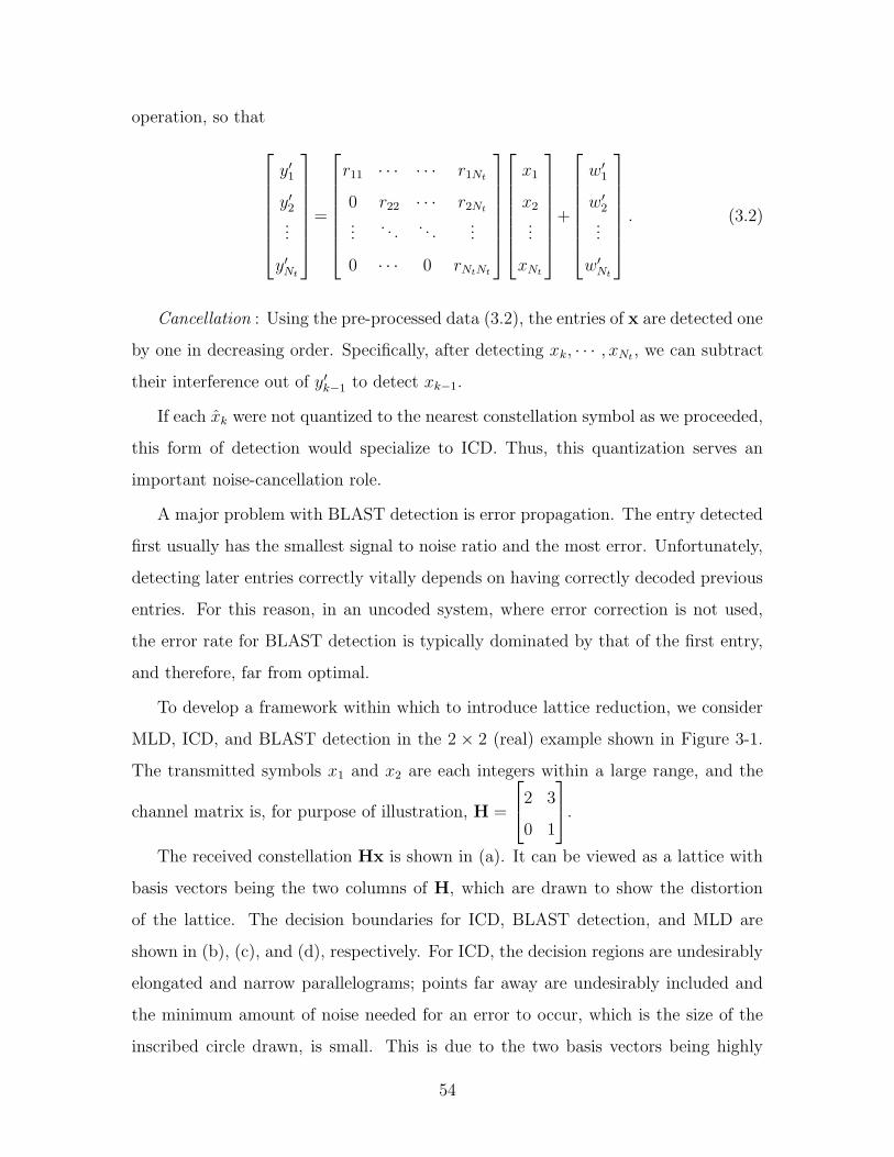
operation, so that
y′1
y′2...
y′Nt
=
r11 · · · · · · r1Nt
0 r22 · · · r2Nt
.... . . . . .
...
0 · · · 0 rNtNt
x1
x2...
xNt
+
w′1
w′2...
w′Nt
. (3.2)
Cancellation : Using the pre-processed data (3.2), the entries of x are detected one
by one in decreasing order. Specifically, after detecting xk, · · · , xNt, we can subtract
their interference out of y′k−1 to detect xk−1.
If each xk were not quantized to the nearest constellation symbol as we proceeded,
this form of detection would specialize to ICD. Thus, this quantization serves an
important noise-cancellation role.
A major problem with BLAST detection is error propagation. The entry detected
first usually has the smallest signal to noise ratio and the most error. Unfortunately,
detecting later entries correctly vitally depends on having correctly decoded previous
entries. For this reason, in an uncoded system, where error correction is not used,
the error rate for BLAST detection is typically dominated by that of the first entry,
and therefore, far from optimal.
To develop a framework within which to introduce lattice reduction, we consider
MLD, ICD, and BLAST detection in the 2 × 2 (real) example shown in Figure 3-1.
The transmitted symbols x1 and x2 are each integers within a large range, and the
channel matrix is, for purpose of illustration, H =
2 3
0 1
.
The received constellation Hx is shown in (a). It can be viewed as a lattice with
basis vectors being the two columns of H, which are drawn to show the distortion
of the lattice. The decision boundaries for ICD, BLAST detection, and MLD are
shown in (b), (c), and (d), respectively. For ICD, the decision regions are undesirably
elongated and narrow parallelograms; points far away are undesirably included and
the minimum amount of noise needed for an error to occur, which is the size of the
inscribed circle drawn, is small. This is due to the two basis vectors being highly
54
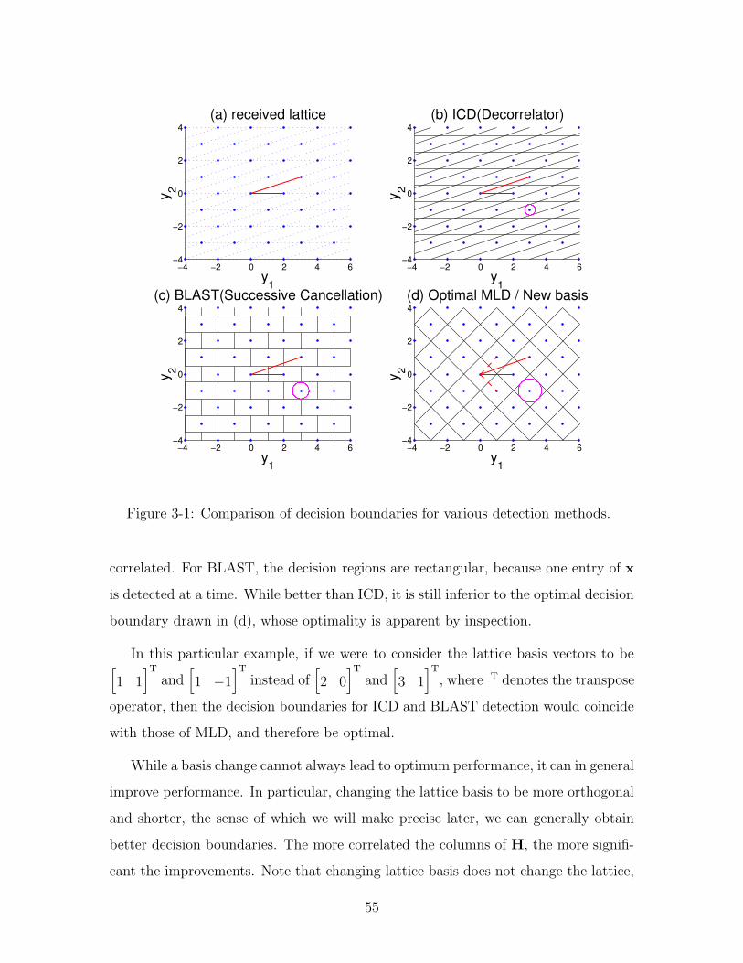
−4 −2 0 2 4 6−4
−2
0
2
4(a) received lattice
y1
y 2
−4 −2 0 2 4 6−4
−2
0
2
4(b) ICD(Decorrelator)
y1
y 2
−4 −2 0 2 4 6−4
−2
0
2
4(c) BLAST(Successive Cancellation)
y1
y 2
−4 −2 0 2 4 6−4
−2
0
2
4(d) Optimal MLD / New basis
y1
y 2
Figure 3-1: Comparison of decision boundaries for various detection methods.
correlated. For BLAST, the decision regions are rectangular, because one entry of x
is detected at a time. While better than ICD, it is still inferior to the optimal decision
boundary drawn in (d), whose optimality is apparent by inspection.
In this particular example, if we were to consider the lattice basis vectors to be[1 1
]Tand
[1 −1
]Tinstead of
[2 0
]Tand
[3 1
]T, where T denotes the transpose
operator, then the decision boundaries for ICD and BLAST detection would coincide
with those of MLD, and therefore be optimal.
While a basis change cannot always lead to optimum performance, it can in general
improve performance. In particular, changing the lattice basis to be more orthogonal
and shorter, the sense of which we will make precise later, we can generally obtain
better decision boundaries. The more correlated the columns of H, the more signifi-
cant the improvements. Note that changing lattice basis does not change the lattice,
55
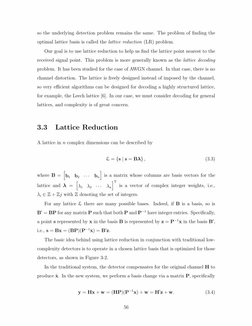
so the underlying detection problem remains the same. The problem of finding the
optimal lattice basis is called the lattice reduction (LR) problem.
Our goal is to use lattice reduction to help us find the lattice point nearest to the
received signal point. This problem is more generally known as the lattice decoding
problem. It has been studied for the case of AWGN channel. In that case, there is no
channel distortion. The lattice is freely designed instead of imposed by the channel,
so very efficient algorithms can be designed for decoding a highly structured lattice,
for example, the Leech lattice [6]. In our case, we must consider decoding for general
lattices, and complexity is of great concern.
3.3 Lattice Reduction
A lattice in n complex dimensions can be described by
L = s | s = Bλ , (3.3)
where B =[b1 b2 · · · bn
]is a matrix whose columns are basis vectors for the
lattice and λ =[λ1 λ2 · · · λn
]Tis a vector of complex integer weights, i.e.,
λi ∈ Z + Zj with Z denoting the set of integers.
For any lattice L there are many possible bases. Indeed, if B is a basis, so is
B′ = BP for any matrixP such that bothP andP−1 have integer entries. Specifically,
a point s represented by x in the basis B is represented by z = P−1x in the basis B′,
i.e., s = Bx = (BP)(P−1x) = B′z.
The basic idea behind using lattice reduction in conjunction with traditional low-
complexity detectors is to operate in a chosen lattice basis that is optimized for those
detectors, as shown in Figure 3-2.
In the traditional system, the detector compensates for the original channel H to
produce x. In the new system, we perform a basis change via a matrix P, specifically
y = Hx+w = (HP)(P−1x) +w = H′z+w. (3.4)
56
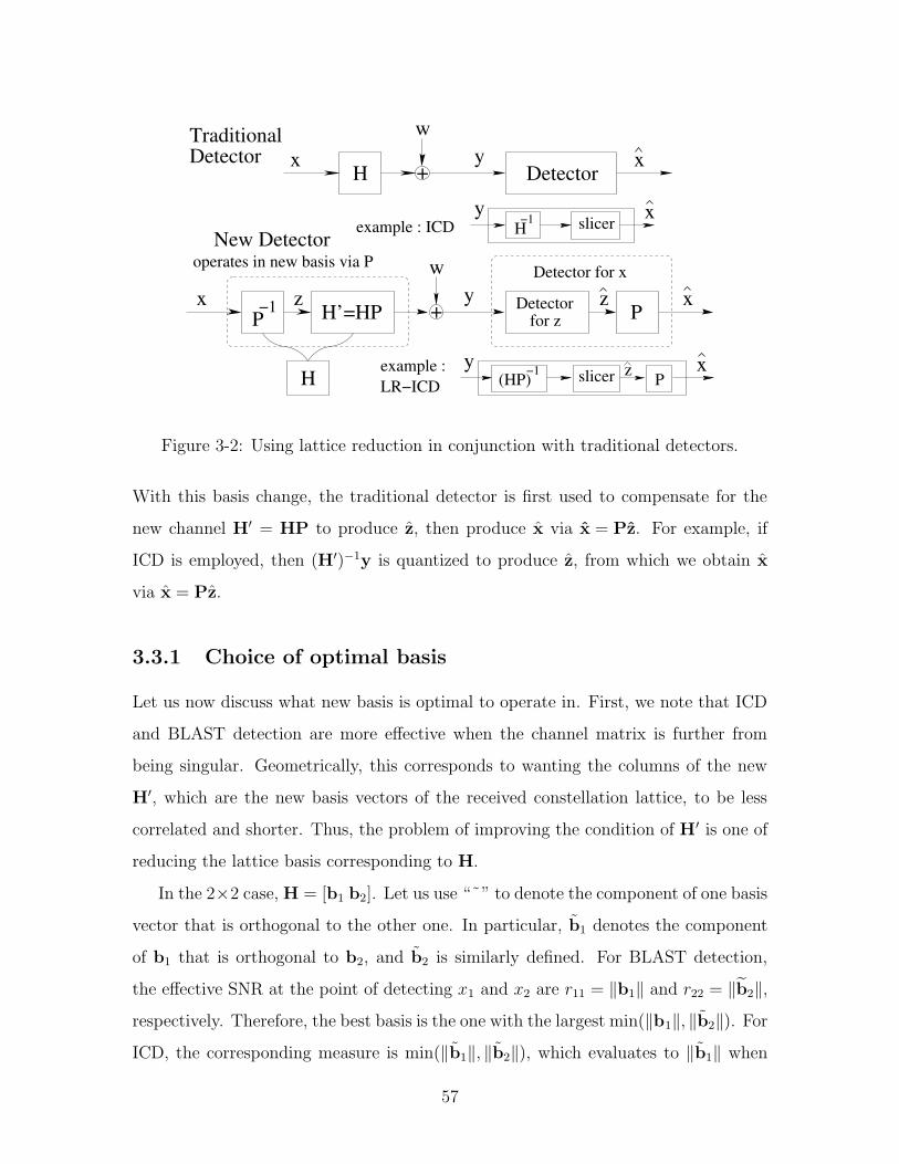
+
−1H slicer
xexample : ICD
y
x
H’=HPz x
x
+
H Detectorx y
TraditionalDetector
Detectorfor zP
−1y
Px z
H Pslicer(HP)−1y z
Detector for x
New Detector
example :LR−ICD
operates in new basis via P
w
w
Figure 3-2: Using lattice reduction in conjunction with traditional detectors.
With this basis change, the traditional detector is first used to compensate for the
new channel H′ = HP to produce z, then produce x via x = Pz. For example, if
ICD is employed, then (H′)−1y is quantized to produce z, from which we obtain x
via x = Pz.
3.3.1 Choice of optimal basis
Let us now discuss what new basis is optimal to operate in. First, we note that ICD
and BLAST detection are more effective when the channel matrix is further from
being singular. Geometrically, this corresponds to wanting the columns of the new
H′, which are the new basis vectors of the received constellation lattice, to be less
correlated and shorter. Thus, the problem of improving the condition of H′ is one of
reducing the lattice basis corresponding to H.
In the 2×2 case,H = [b1 b2]. Let us use “˜” to denote the component of one basis
vector that is orthogonal to the other one. In particular, b1 denotes the component
of b1 that is orthogonal to b2, and b2 is similarly defined. For BLAST detection,
the effective SNR at the point of detecting x1 and x2 are r11 = ‖b1‖ and r22 = ‖b2‖,respectively. Therefore, the best basis is the one with the largest min(‖b1‖, ‖b2‖). ForICD, the corresponding measure is min(‖b1‖, ‖b2‖), which evaluates to ‖b1‖ when
57
‖b1‖ ≤ ‖b2‖. With these criteria, we show that the optimal basis for both detection
methods is (u,v), where u is the shortest (non-zero) vector in the lattice and v is the
shortest vector that is not a multiple of u. This is done in the next two lemmas, for
BLAST detection and ICD, respectively.
Lemma 3.1 (Optimality for BLAST) Given a two dimensional lattice with basis
(u,v). If u is the shortest (non-zero) vector in the lattice and v is the shortest vector
that is not a multiple of u, then for any other basis of the lattice (b1,b2),
min(‖u‖, ‖v‖) ≥ min(‖b1‖, ‖b2‖). (3.5)
Proof:
This proof can be done in two parts:
1) ‖u‖ ≥ min(‖b1‖, ‖b2‖) and 2) ‖v‖ ≥ min(‖b1‖, ‖b2‖).
1) Since (b1,b2) is a lattice basis, u can be written as u = c1b1 + c2b2, where c1 andc2 are not both zero and c1, c2 ∈ Z+ Zj.If c2 6= 0, then |c2| ≥ 1. The component of u orthogonal to b1 is c2b2. Therefore,
‖u‖ ≥ ‖c2b2‖ ≥ ‖b2‖ ≥ min(‖b1‖, ‖b2‖).
If c2 = 0, then u = c1b1, where c1 6= 0 and |c1| ≥ 1. Therefore,
‖u‖ = |c1| · ‖b1‖ ≥ 1 · ‖b1‖u shortest⇒ ‖u‖ ≤ ‖b1‖
=⇒ ‖u‖ = ‖b1‖ ≥ min(‖b1‖, ‖b2‖).
2) Since (u,v) and (b1,b2) are both bases of the same lattice, ‖u‖ · ‖v‖ = ‖b1‖ · ‖b2‖,both being volume of a unit cell of the lattice. Therefore,
u shortest⇒ ‖u‖ ≤ ‖b1‖ =⇒ ‖v‖ ≥ ‖b2‖ ≥ min(‖b1‖, ‖b2‖).
Lemma 3.2 (Optimality for ICD) Given a two dimensional lattice with basis (u,v).
If u is the shortest (non-zero) vector in the lattice and v is the shortest vector that is
not a multiple of u, then for any other basis of the lattice (b1,b2) with ‖b1‖ ≤ ‖b2‖,
‖u‖ ≥ ‖b1‖. (3.6)
58
Proof:
This proof is done by contradiction. Suppose ‖u‖ < ‖b1‖. Since (u,v) and (b1,b2) areboth bases of the same lattice, ‖u‖ · ‖v‖ = ‖b1‖ · ‖b2‖, again, both being volume of a unitcell of the lattice.
‖u‖ < ‖b1‖ =⇒ ‖v‖ > ‖b2‖ ≥ ‖b1‖=⇒ Both b1 and b2 are multiples of u.
=⇒ (b1,b2) can not be a basis.
=⇒ contradiction
This utilizes the condition that v is the shortest vector that is not a multiple of u. Therefore,b1 and b2 can not both be shorter than v and form a basis.
3.3.2 Reduction Algorithm
Given an original set of basis vectors (b1,b2) for a lattice with ‖b1‖ ≤ ‖b2‖, we
develop an iterative algorithm to progressively reduce their correlation and converge
to the desired basis vectors (u,v).
One intuitive way to reduce the correlation between two lattice basis vectors is to
subtract integer copies of the shorter vector out of the longer one. Let b′2 = (b2−nb1)be the replacement for b2. The parameter n should be chosen so as to minimize the
correlation between b1 and b′2, i.e.,
n∗ = argminn∈Z+Zj
|〈b1,b2 − nb1〉| = argminn∈Z+Zj
|〈b1,b2〉 − n‖b1‖2| =⌊〈b1,b2〉‖b1‖2
⌉, (3.7)
where the function b·e rounds its argument to the nearest integer. For complex
arguments, real and imaginary parts are rounded separately. And to avoid ambiguity,
half integers are rounded to even integers. Note that this choice of n given by (3.7)
59
also minimizes the norm of b′2.
argminn∈Z+Zj
‖b2 − nb1‖2
= argminn∈Z+Zj
|n|2‖b1‖2 − 2Ren〈b2,b1〉+ ‖b2‖2
= argminn=nr+nij
(n2r + n2i )‖b1‖2 − 2nr Re〈b1,b2〉 − 2ni Im〈b1,b2〉+ ‖b2‖2
=
⌊〈b1,b2〉‖b1‖2
⌉.
The resulting correlation after replacing b2 with b′2 is
〈b1,b′2〉 =
⟨b1,
(b2 −
⌊〈b1,b2〉‖b1‖2
⌉b1
)⟩
=
(〈b1,b2〉‖b1‖2
−⌊〈b1,b2〉‖b1‖2
⌉)· ‖b1‖2.
Since the rounding errors for real and imaginary parts are each no more than 1/2, we
have
|Re〈b1,b′2〉| ≤1
2‖b1‖2 and | Im〈b1,b′2〉| ≤
1
2‖b1‖2. (3.8)
After replacing b2 with the optimal b′2, if this new b2 is shorter than b1, we swap
them and then check whether further subtraction is possible.
Summarizing, the algorithm is as follows:
1. Check the correlation. If |Re〈b1,b2〉| ≤ 12‖b1‖2 and | Im〈b1,b2〉| ≤ 1
2‖b1‖2,
stop. Otherwise, replace b2 with b2 −⌊〈b1,b2〉‖b1‖2
⌉b1 and go to step 2.
2. Check their lengths. If ‖b2‖ > ‖b1‖, stop. Otherwise, swap them and go to
step 1.
When this iterative procedure stops, the resulting basis has the properties ‖b1‖ ≤‖b2‖, |Re〈b1,b2〉| ≤ 1
2‖b1‖2 and | Im〈b1,b2〉| ≤ 1
2‖b1‖2. It follows that basis
vectors with these properties are the ones we desire, as we show next.
60
Lemma 3.3 Given a two dimensional lattice with basis vectors u and v. If ‖u‖ ≤ ‖v‖,|Re〈u,v〉| ≤ 1
2‖u‖2, and |Im〈u,v〉| ≤ 1
2‖u‖2, then
1) u is the shortest (non-zero) vector in the lattice.
2) v is the shortest vector that is not a multiple of u.
Proof:
1) Since (u,v) is a lattice basis, any vector s in the lattice can be written as s = au+ bv,with a, b ∈ Z+ Zj. Let ar = Rea, ai = Ima, br = Reb, bi = Imb. We have,
‖s‖2 = ‖au+ bv‖2
= |a|2‖u‖2 + |b|2‖v‖2 + 2Rea†b〈u,v〉≥ (a2r + a2i + b2r + b2i −|arbr + aibi|−|aibr − arbi|)‖u‖2
≥ ‖u‖2 when ar, ai, br, bi are not all 0,
The last step uses the identities, for a, b, c, d ∈ Z,
• a2 + b2 + c2 + d2 ≥ |ac|+ |bd|+ |bc|+ |ad| with equality iff |a| = |b| = |c| = |d|.
• |ac|+ |bd| ≥ |ac+ bd| with equality iff abcd ≥ 0.
• |bc|+ |ad| ≥ |bc− ad| with equality iff abcd ≤ 0.
2) Any vector s in the lattice that is not a multiple of u can be written as s = au+ bv,a, b ∈ Z+ Zj, and b 6= 0.
‖s‖2 = ‖au+ bv‖2
= |b|2(‖v‖2 − ‖u‖2
)+ |a|2‖u‖2 + |b|2‖u‖2 + 2Rea†b〈u,v〉︸ ︷︷ ︸
≥ |b|2(‖v‖2 − ‖u‖2
)+ ‖u‖2 +
(‖v‖2 − ‖v‖2
)
= (|b|2 − 1) · (‖v‖2 − ‖u‖2) + ‖v‖2
≥ ‖v‖2 because b 6= 0
3.3.3 Convergence and Complexity
In this section, let us discuss the convergence of the iterative algorithm proposed
as well as its complexity. In other words, does this procedure end and how many
iterations does it take?
It is clear that the procedure does end. In particular, after each iteration, the
lengths of both basis vectors decrease (at least one decreases strictly); otherwise,
61
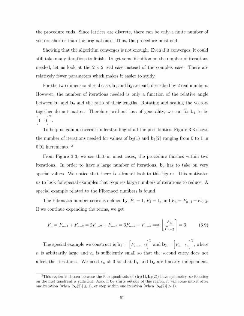
the procedure ends. Since lattices are discrete, there can be only a finite number of
vectors shorter than the original ones. Thus, the procedure must end.
Showing that the algorithm converges is not enough. Even if it converges, it could
still take many iterations to finish. To get some intuition on the number of iterations
needed, let us look at the 2 × 2 real case instead of the complex case. There are
relatively fewer parameters which makes it easier to study.
For the two dimensional real case, b1 and b2 are each described by 2 real numbers.
However, the number of iterations needed is only a function of the relative angle
between b1 and b2 and the ratio of their lengths. Rotating and scaling the vectors
together do not matter. Therefore, without loss of generality, we can fix b1 to be[1 0
]T.
To help us gain an overall understanding of all the possibilities, Figure 3-3 shows
the number of iterations needed for values of b2(1) and b2(2) ranging from 0 to 1 in
0.01 increments. 2
From Figure 3-3, we see that in most cases, the procedure finishes within two
iterations. In order to have a large number of iterations, b2 has to take on very
special values. We notice that there is a fractal look to this figure. This motivates
us to look for special examples that requires large numbers of iterations to reduce. A
special example related to the Fibonacci numbers is found.
The Fibonacci number series is defined by, F1 = 1, F2 = 1, and Fn = Fn−1+Fn−2.
If we continue expending the terms, we get
Fn = Fn−1 + Fn−2 = 2Fn−2 + Fn−3 = 3Fn−2 − Fn−4 =⇒⌊FnFn−2
⌉= 3. (3.9)
The special example we construct is b1 =[Fn−2 0
]Tand b2 =
[Fn εn
]T, where
n is arbitrarily large and εn is sufficiently small so that the second entry does not
affect the iterations. We need εn 6= 0 so that b1 and b2 are linearly independent.
2This region is chosen because the four quadrants of (b2(1),b2(2)) have symmetry, so focusingon the first quadrant is sufficient. Also, if b2 starts outside of this region, it will come into it afterone iteration (when |b2(2)| ≤ 1), or stop within one iteration (when |b2(2)| > 1).
62
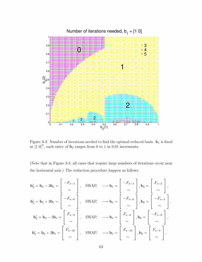
0 0.1 0.2 0.3 0.4 0.5 0.6 0.7 0.8 0.9 10
0.1
0.2
0.3
0.4
0.5
0.6
0.7
0.8
0.9
1
0
1
2
222
345
Number of iterations needed, b1 = [1 0]
b2(1)
b 2(2)
Figure 3-3: Number of iterations needed to find the optimal reduced basis. b1 is fixedat [1 0]T, each entry of b2 ranges from 0 to 1 in 0.01 increments.
(Note that in Figure 3-3, all cases that require large numbers of iterations occur near
the horizontal axis.) The reduction procedure happen as follows.
b′2 = b2 − 3b1 =
−Fn−4
∼
, SWAP, −→ b1 =
−Fn−4
∼
,b2 =
Fn−2
∼
,
b′2 = b2 + 3b1 =
−Fn−6
∼
, SWAP, −→ b1 =
−Fn−6
∼
,b2 =
−Fn−4
∼
,
b′2 = b2 − 3b1 =
Fn−8
∼
, SWAP, −→ b1 =
Fn−8
∼
,b2 =
−Fn−6
∼
,
b′2 = b2 + 3b1 =
Fn−10
∼
, SWAP, −→ b1 =
Fn−10
∼
,b2 =
Fn−8
∼
,
63
and so on. By choosing n to be arbitrarily large, we have constructed an example
that requires arbitrarily many iterations to finish.
In conclusion, the number of iterations needed is fixed but arbitrarily large. Given
any initial basis, it takes a fixed number of iterations to finish. However, given any
number n, there exist bases that require more then n steps to reduce. In most cases,
it takes very few iterations to finish; needing more is increasingly unlikely.
In the next two sections we examine the effects of using lattice reduction with
traditional detectors. Let us use LR-ICD and LR-BLAST to refer to the detection
schemes that combine lattice reduction with ICD and BLAST detection respectively.
3.4 Gaussian Channels
In this section we develop results for a fixed channel matrix H.
3.4.1 Complexity
The incremental complexity inherent in the use of lattice reduction is determined by
the number of iterations required to reduce the basis. As we saw in section 3.3.3,
for 2 × 2 channels, the number of iterations needed is small, less than two, for most
channels. However, it is possible to construct examples that take arbitrarily many
iterations to finish. The worst case is unbounded, but highly unlikely. Therefore,
practically speaking, if we were to perform low complexity detection in this new basis
as we proposed, the overhead associated with looking for the optimal basis would be
very low. Thus, the overall algorithm has low complexity.
3.4.2 Performance
These new detection methods lead to decision regions (and thus performance) much
closer to that of MLD, as we now develop.
Figure 3-4 shows a comparison of the decision regions for MLD and LR-ICD. It is
drawn for a 2× 2 real example for illustration purpose. The MLD decision region is
64
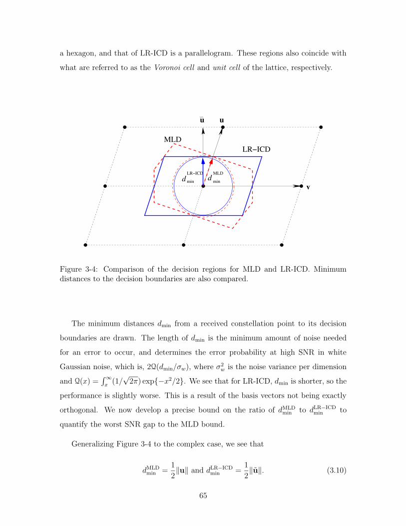
a hexagon, and that of LR-ICD is a parallelogram. These regions also coincide with
what are referred to as the Voronoi cell and unit cell of the lattice, respectively.
u
v
u
MLD
dLR−ICD
mind min
MLD
LR−ICD
Figure 3-4: Comparison of the decision regions for MLD and LR-ICD. Minimumdistances to the decision boundaries are also compared.
The minimum distances dmin from a received constellation point to its decision
boundaries are drawn. The length of dmin is the minimum amount of noise needed
for an error to occur, and determines the error probability at high SNR in white
Gaussian noise, which is, 2Q(dmin/σw), where σ2w is the noise variance per dimension
and Q(x) =∫∞x(1/√2π) exp−x2/2. We see that for LR-ICD, dmin is shorter, so the
performance is slightly worse. This is a result of the basis vectors not being exactly
orthogonal. We now develop a precise bound on the ratio of dMLDmin to dLR−ICDmin to
quantify the worst SNR gap to the MLD bound.
Generalizing Figure 3-4 to the complex case, we see that
dMLDmin =
1
2‖u‖ and dLR−ICDmin =
1
2‖u‖. (3.10)
65
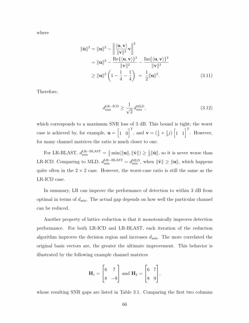
where
‖u‖2 = ‖u‖2 −∥∥∥∥〈u,v〉‖v‖2 v
∥∥∥∥2
= ‖u‖2 − Re〈u,v〉2‖v‖2 − Im〈u,v〉2
‖v‖2
≥ ‖u‖2(1− 1
4− 1
4
)=
1
2‖u‖2. (3.11)
Therefore,
dLR−ICDmin ≥ 1√2dMLDmin , (3.12)
which corresponds to a maximum SNR loss of 3 dB. This bound is tight; the worst
case is achieved by, for example, u =[1 0
]T, and v = (1
2+ 1
2j)[1 1
]T. However,
for many channel matrices the ratio is much closer to one.
For LR-BLAST, dLR−BLASTmin = 12min(‖u‖, ‖v‖) ≥ 1
2‖u‖, so it is never worse than
LR-ICD. Comparing to MLD, dLR−BLASTmin = dMLDmin , when ‖v‖ ≥ ‖u‖, which happens
quite often in the 2 × 2 case. However, the worst-case ratio is still the same as the
LR-ICD case.
In summary, LR can improve the performance of detection to within 3 dB from
optimal in terms of dmin. The actual gap depends on how well the particular channel
can be reduced.
Another property of lattice reduction is that it monotonically improves detection
performance. For both LR-ICD and LR-BLAST, each iteration of the reduction
algorithm improves the decision region and increases dmin. The more correlated the
original basis vectors are, the greater the ultimate improvement. This behavior is
illustrated by the following example channel matrices
H1 =
6 7
8 −9
and H2 =
6 7
8 9
,
whose resulting SNR gaps are listed in Table 3.1. Comparing the first two columns
66
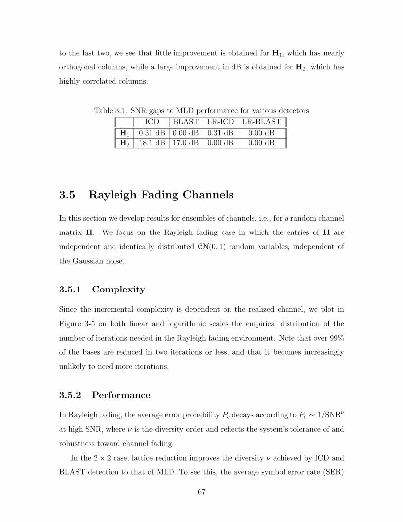
to the last two, we see that little improvement is obtained for H1, which has nearly
orthogonal columns, while a large improvement in dB is obtained for H2, which has
highly correlated columns.
Table 3.1: SNR gaps to MLD performance for various detectors
ICD BLAST LR-ICD LR-BLAST
H1 0.31 dB 0.00 dB 0.31 dB 0.00 dBH2 18.1 dB 17.0 dB 0.00 dB 0.00 dB
3.5 Rayleigh Fading Channels
In this section we develop results for ensembles of channels, i.e., for a random channel
matrix H. We focus on the Rayleigh fading case in which the entries of H are
independent and identically distributed CN(0, 1) random variables, independent of
the Gaussian noise.
3.5.1 Complexity
Since the incremental complexity is dependent on the realized channel, we plot in
Figure 3-5 on both linear and logarithmic scales the empirical distribution of the
number of iterations needed in the Rayleigh fading environment. Note that over 99%
of the bases are reduced in two iterations or less, and that it becomes increasingly
unlikely to need more iterations.
3.5.2 Performance
In Rayleigh fading, the average error probability Pe decays according to Pe ∼ 1/SNRν
at high SNR, where ν is the diversity order and reflects the system’s tolerance of and
robustness toward channel fading.
In the 2× 2 case, lattice reduction improves the diversity ν achieved by ICD and
BLAST detection to that of MLD. To see this, the average symbol error rate (SER)
67
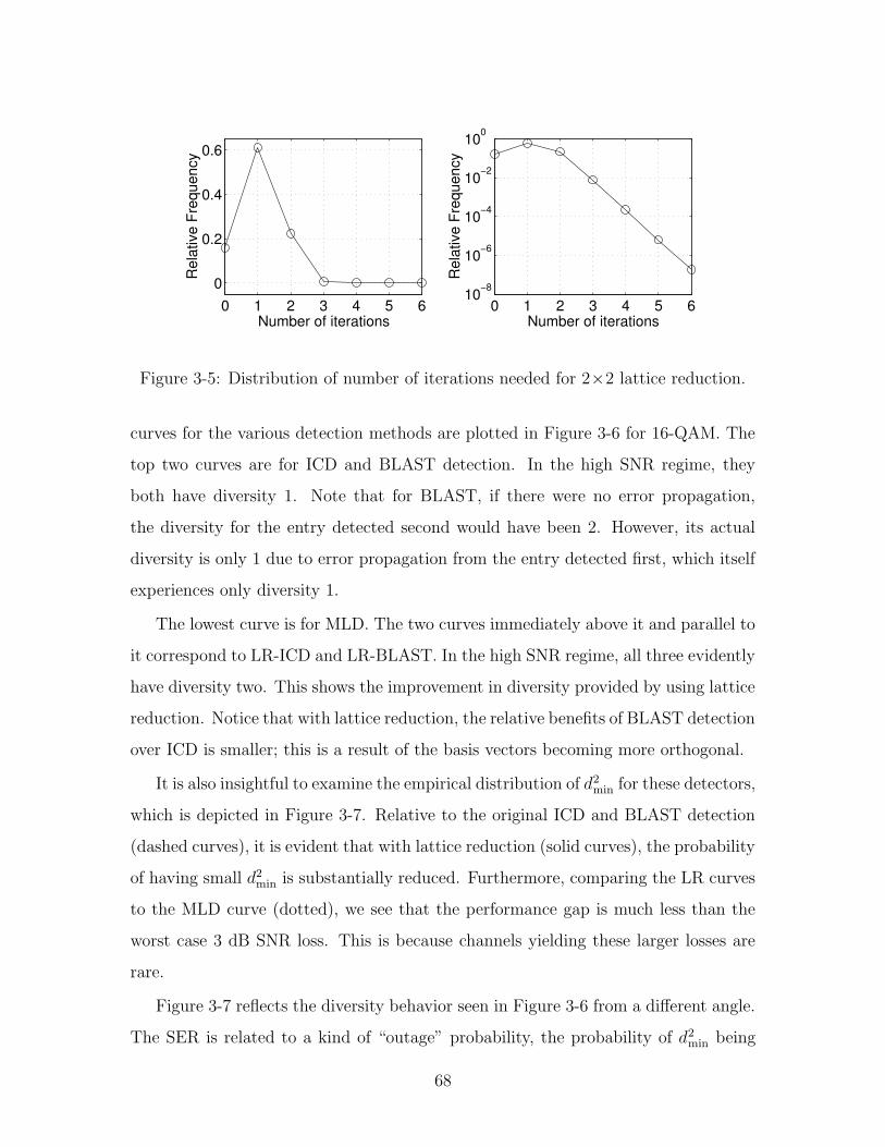
0 1 2 3 4 5 60
0.2
0.4
0.6
Number of iterations
Rel
ativ
e Fr
eque
ncy
0 1 2 3 4 5 610
−8
10−6
10−4
10−2
100
Number of iterations
Rel
ativ
e Fr
eque
ncy
Figure 3-5: Distribution of number of iterations needed for 2×2 lattice reduction.
curves for the various detection methods are plotted in Figure 3-6 for 16-QAM. The
top two curves are for ICD and BLAST detection. In the high SNR regime, they
both have diversity 1. Note that for BLAST, if there were no error propagation,
the diversity for the entry detected second would have been 2. However, its actual
diversity is only 1 due to error propagation from the entry detected first, which itself
experiences only diversity 1.
The lowest curve is for MLD. The two curves immediately above it and parallel to
it correspond to LR-ICD and LR-BLAST. In the high SNR regime, all three evidently
have diversity two. This shows the improvement in diversity provided by using lattice
reduction. Notice that with lattice reduction, the relative benefits of BLAST detection
over ICD is smaller; this is a result of the basis vectors becoming more orthogonal.
It is also insightful to examine the empirical distribution of d2min for these detectors,
which is depicted in Figure 3-7. Relative to the original ICD and BLAST detection
(dashed curves), it is evident that with lattice reduction (solid curves), the probability
of having small d2min is substantially reduced. Furthermore, comparing the LR curves
to the MLD curve (dotted), we see that the performance gap is much less than the
worst case 3 dB SNR loss. This is because channels yielding these larger losses are
rare.
Figure 3-7 reflects the diversity behavior seen in Figure 3-6 from a different angle.
The SER is related to a kind of “outage” probability, the probability of d2min being
68
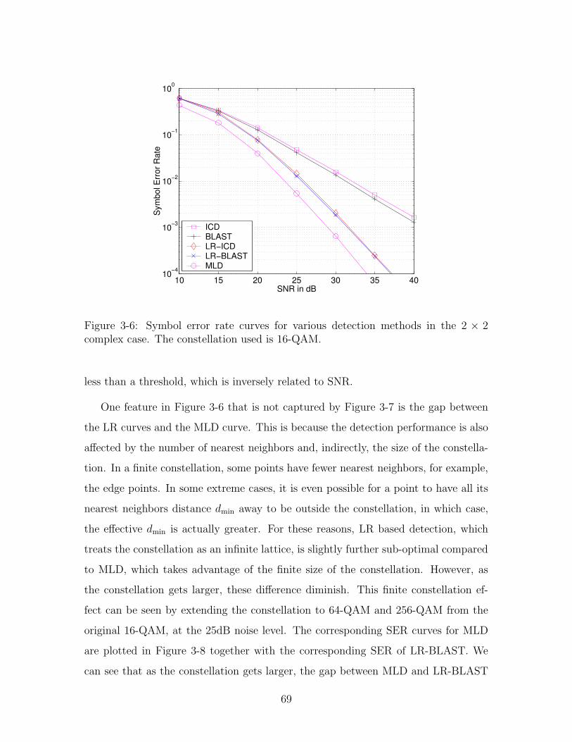
10 15 20 25 30 35 4010
−4
10−3
10−2
10−1
100
SNR in dB
Sym
bol E
rror
Rat
e
ICDBLASTLR−ICDLR−BLASTMLD
Figure 3-6: Symbol error rate curves for various detection methods in the 2 × 2complex case. The constellation used is 16-QAM.
less than a threshold, which is inversely related to SNR.
One feature in Figure 3-6 that is not captured by Figure 3-7 is the gap between
the LR curves and the MLD curve. This is because the detection performance is also
affected by the number of nearest neighbors and, indirectly, the size of the constella-
tion. In a finite constellation, some points have fewer nearest neighbors, for example,
the edge points. In some extreme cases, it is even possible for a point to have all its
nearest neighbors distance dmin away to be outside the constellation, in which case,
the effective dmin is actually greater. For these reasons, LR based detection, which
treats the constellation as an infinite lattice, is slightly further sub-optimal compared
to MLD, which takes advantage of the finite size of the constellation. However, as
the constellation gets larger, these difference diminish. This finite constellation ef-
fect can be seen by extending the constellation to 64-QAM and 256-QAM from the
original 16-QAM, at the 25dB noise level. The corresponding SER curves for MLD
are plotted in Figure 3-8 together with the corresponding SER of LR-BLAST. We
can see that as the constellation gets larger, the gap between MLD and LR-BLAST
69
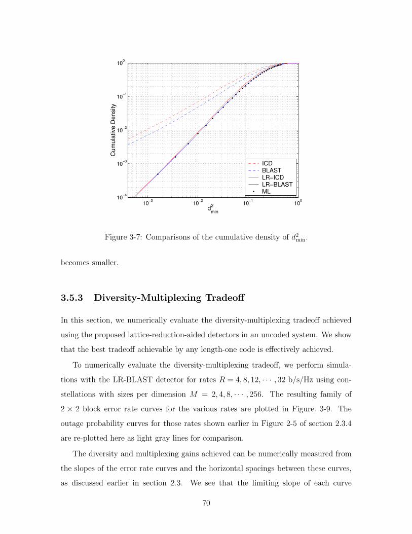
10−3
10−2
10−1
100
10−4
10−3
10−2
10−1
100
dmin2
Cum
ulat
ive
Den
sity
ICDBLASTLR−ICDLR−BLASTML
Figure 3-7: Comparisons of the cumulative density of d2min.
becomes smaller.
3.5.3 Diversity-Multiplexing Tradeoff
In this section, we numerically evaluate the diversity-multiplexing tradeoff achieved
using the proposed lattice-reduction-aided detectors in an uncoded system. We show
that the best tradeoff achievable by any length-one code is effectively achieved.
To numerically evaluate the diversity-multiplexing tradeoff, we perform simula-
tions with the LR-BLAST detector for rates R = 4, 8, 12, · · · , 32 b/s/Hz using con-
stellations with sizes per dimension M = 2, 4, 8, · · · , 256. The resulting family of
2 × 2 block error rate curves for the various rates are plotted in Figure. 3-9. The
outage probability curves for those rates shown earlier in Figure 2-5 of section 2.3.4
are re-plotted here as light gray lines for comparison.
The diversity and multiplexing gains achieved can be numerically measured from
the slopes of the error rate curves and the horizontal spacings between these curves,
as discussed earlier in section 2.3. We see that the limiting slope of each curve
70
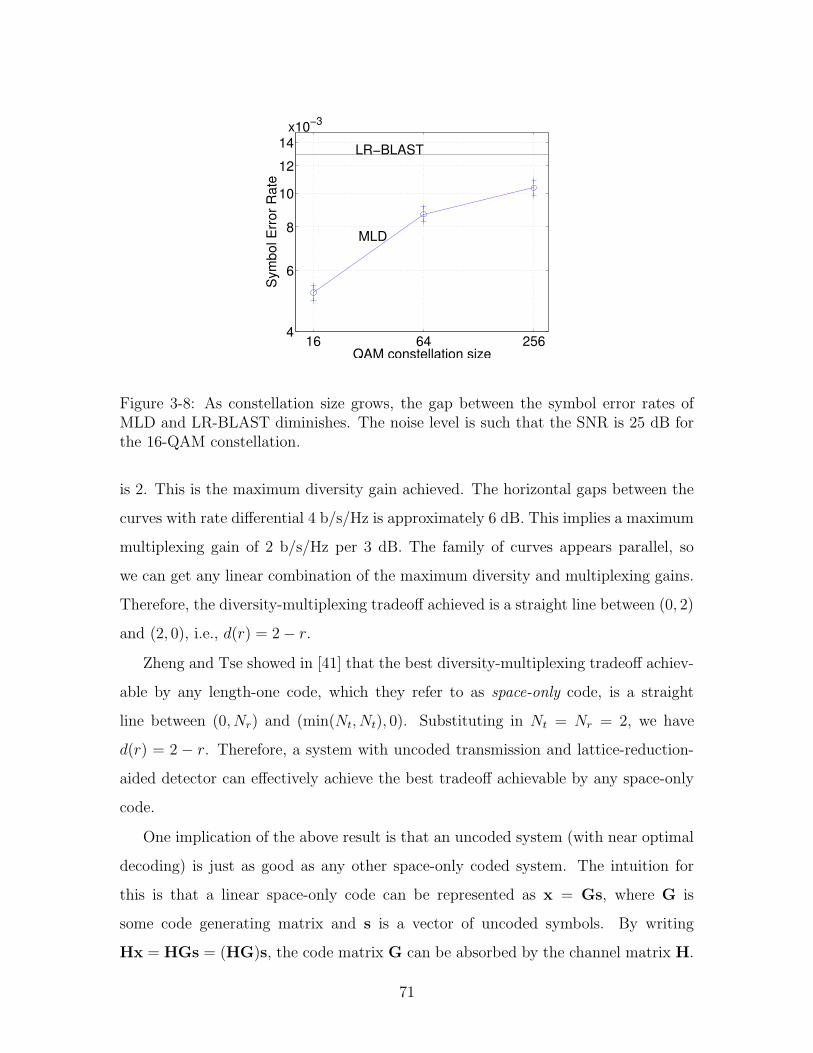
16 64 2564
6
8
10
12
14 LR−BLAST
MLD
QAM constellation size
Sym
bol E
rror
Rat
e
x10−3
Figure 3-8: As constellation size grows, the gap between the symbol error rates ofMLD and LR-BLAST diminishes. The noise level is such that the SNR is 25 dB forthe 16-QAM constellation.
is 2. This is the maximum diversity gain achieved. The horizontal gaps between the
curves with rate differential 4 b/s/Hz is approximately 6 dB. This implies a maximum
multiplexing gain of 2 b/s/Hz per 3 dB. The family of curves appears parallel, so
we can get any linear combination of the maximum diversity and multiplexing gains.
Therefore, the diversity-multiplexing tradeoff achieved is a straight line between (0, 2)
and (2, 0), i.e., d(r) = 2− r.
Zheng and Tse showed in [41] that the best diversity-multiplexing tradeoff achiev-
able by any length-one code, which they refer to as space-only code, is a straight
line between (0, Nr) and (min(Nt, Nt), 0). Substituting in Nt = Nr = 2, we have
d(r) = 2 − r. Therefore, a system with uncoded transmission and lattice-reduction-
aided detector can effectively achieve the best tradeoff achievable by any space-only
code.
One implication of the above result is that an uncoded system (with near optimal
decoding) is just as good as any other space-only coded system. The intuition for
this is that a linear space-only code can be represented as x = Gs, where G is
some code generating matrix and s is a vector of uncoded symbols. By writing
Hx = HGs = (HG)s, the code matrix G can be absorbed by the channel matrix H.
71
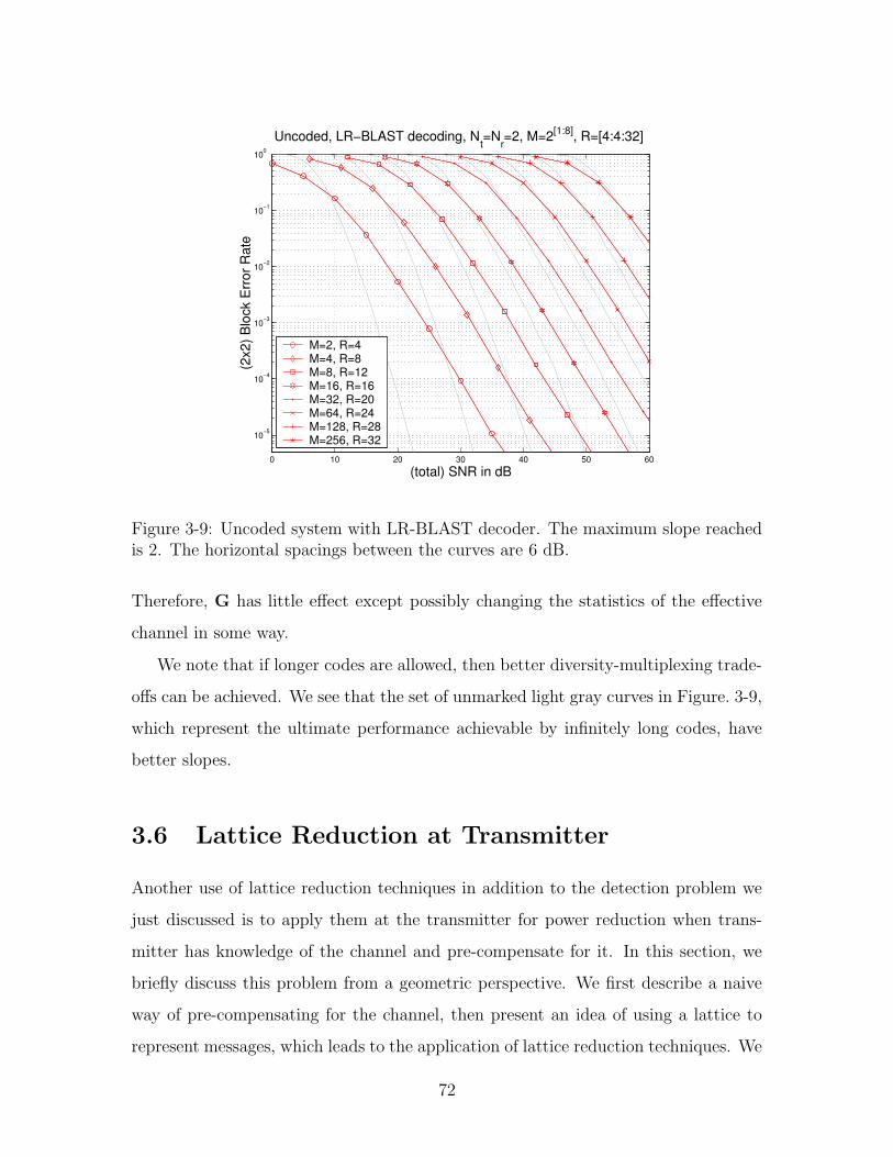
0 10 20 30 40 50 60
10−5
10−4
10−3
10−2
10−1
100
(total) SNR in dB
(2x2
) Blo
ck E
rror
Rat
e
Uncoded, LR−BLAST decoding, Nt=N
r=2, M=2[1:8], R=[4:4:32]
M=2, R=4M=4, R=8M=8, R=12M=16, R=16M=32, R=20M=64, R=24M=128, R=28M=256, R=32
Figure 3-9: Uncoded system with LR-BLAST decoder. The maximum slope reachedis 2. The horizontal spacings between the curves are 6 dB.
Therefore, G has little effect except possibly changing the statistics of the effective
channel in some way.
We note that if longer codes are allowed, then better diversity-multiplexing trade-
offs can be achieved. We see that the set of unmarked light gray curves in Figure. 3-9,
which represent the ultimate performance achievable by infinitely long codes, have
better slopes.
3.6 Lattice Reduction at Transmitter
Another use of lattice reduction techniques in addition to the detection problem we
just discussed is to apply them at the transmitter for power reduction when trans-
mitter has knowledge of the channel and pre-compensate for it. In this section, we
briefly discuss this problem from a geometric perspective. We first describe a naive
way of pre-compensating for the channel, then present an idea of using a lattice to
represent messages, which leads to the application of lattice reduction techniques. We
72

only illustrate the basic ideas, the details are left for future development.
When the transmitter has knowledge of the channel, it can pre-compensate for
the distortion by transmitting H−1x instead of x. The resulting received signal is
then y = H(H−1x) + w = x + w. This means that the receiver effectively sees an
AWGN channel, and can detect each entry of x independently without knowing the
channel. This idea is illustrated in Figure 3-10.
Channel
=
Pre−compensate
x−1
H(H x) x−1H x
Figure 3-10: When the transmitter knows the channel, it can pre-compensate for thedistortion by transmittingH−1x, so that the received constellation is the original one.
One problem with pre-multiplying with H−1 is that the resulting constellation
region becomes very elongated, as seen in Figure 3-10. (This effect is similar to the
noise enhancement problem of the inverse channel detector in section 3.2.) Having
an elongated constellation region is inefficient in terms of power usage because it
takes more power to transmit points further from the origin. This suggests that the
constellation region need to be made more circular.
Next, we review an idea of using a set of congruent points, or a lattice, to signal
a message. Later, this will allow us to use lattice reduction techniques to make the
constellation region more circular and reduce the transmit power.
This idea was introduced by Tomlinson and Harishima as part of their transmitter
pre-coding algorithm [19]. A set of points that are congruent modulo the constellation
region are used to represent the same message. as illustrated in Figure 3-11. All points
marked by “” are congruent to the point marked by “+” modulo the constellation
region drawn with solid lines. To transmit the message originally represented only
by “+”, we can now use any of the “”s. Note that the set of “”s together with the
“+” form a lattice. Among all the lattice points, we would pick the one closest to
73

the origin to minimize transmit power. At the receive, if we receive any “”, which is
outside the constellation region, we find its congruent image inside the constellation
region, which is the “+”, and treat it as if the “+” is actually received.
Channel
−1H xo
oo
+
o
o
ooo
+
o
o
oo
o
x
Figure 3-11: At the transmitter, all points that are congruent modulo the constellationregion, which form a lattice, are use to represent the same message. Points labeled“” represent the same message as the point labeled “+”. At the receiver, any “”can be mapped back to “+” via modulo operations.
With this idea of using a lattice to represent the same message, the problem of
minimizing transmit power becomes the problem of finding the nearest point of a
shifted lattice to the origin. This allows us to use lattice reduction techniques.
In Tomlinson-Harishima pre-coding, modulo operations at the transmitter are
performed one dimension at a time, similar to the successive cancellation technique
used in BLAST detection. We will not review it here. It suffice to say that the
resulting constellation region has the same shape as the decision region achieved by
BLAST detection for the same channels shown in Figure 3-1. It improves the power
efficiency but is not optimal.
Let us now look at what constellation region is the most desirable. We can consider
the original transmitted constellation region and its periodically extended copies,
which are drawn in Figure 3-11 with dotted lines, as unit cells of a lattice. The set
of “”s is a shifted version of this lattice. We see that there is exactly one “” in
each unit cell. In fact, if we were to consider other unit cells of this lattice, there
would still be exactly one “o” in each cell, no matter what the unit cell is. Therefore,
by choosing different unit cells as the constellation region, we choose which “” to
transmit. The best constellation region to use is the unit cell with the least second
74
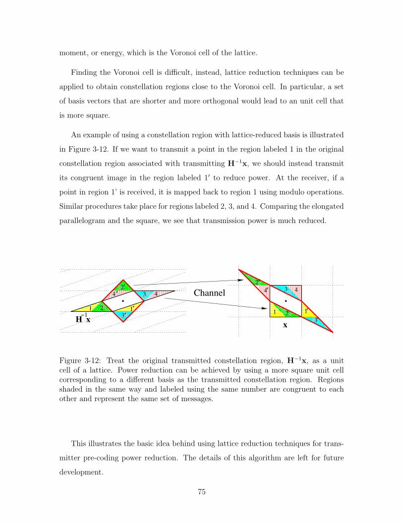
moment, or energy, which is the Voronoi cell of the lattice.
Finding the Voronoi cell is difficult, instead, lattice reduction techniques can be
applied to obtain constellation regions close to the Voronoi cell. In particular, a set
of basis vectors that are shorter and more orthogonal would lead to an unit cell that
is more square.
An example of using a constellation region with lattice-reduced basis is illustrated
in Figure 3-12. If we want to transmit a point in the region labeled 1 in the original
constellation region associated with transmitting H−1x, we should instead transmit
its congruent image in the region labeled 1′ to reduce power. At the receiver, if a
point in region 1’ is received, it is mapped back to region 1 using modulo operations.
Similar procedures take place for regions labeled 2, 3, and 4. Comparing the elongated
parallelogram and the square, we see that transmission power is much reduced.
!!!!!!!!!!!! Channel
−1
xxH
4
1
3
’’
2 1 1
2
2 3
3
3
4 44’
2’
’
’
’
’
1
Figure 3-12: Treat the original transmitted constellation region, H−1x, as a unitcell of a lattice. Power reduction can be achieved by using a more square unit cellcorresponding to a different basis as the transmitted constellation region. Regionsshaded in the same way and labeled using the same number are congruent to eachother and represent the same set of messages.
This illustrates the basic idea behind using lattice reduction techniques for trans-
mitter pre-coding power reduction. The details of this algorithm are left for future
development.
75
3.7 Higher Dimensional Lattice Reduction
In the previous sections, we have demonstrated how using lattice reduction can im-
prove the performance of traditional low complexity detectors to be close to that of
the maximum likelihood detector. We also illustrated how LR can be used at trans-
mitter for pre-coding as well. LR may also potentially be applied to other problems
such as source coding, when the quantization points form a lattice.
The lattice reduction techniques we presented are for the case of two (complex)
dimensions only. We now investigate how feasible and how useful LR might be in
higher dimensional cases. We address issues including what basis should be considered
optimal, what lattice reduction algorithms can be used, what their complexity levels
are, and how well they work when combined with traditional detectors. The main
goal is to point out existing work on lattice reduction theory and discuss them.
Generally speaking, the lattice reduction problem is NP-hard in the dimension
of the lattice. Conway and Sloane [6] expressed their feeling toward this type of
problems as, anything associated with high dimensional lattice is hard except finding
its determinant (the volume of a unit cell). For example, finding the covering radius
has proven to be NP-hard, while finding the packing radius or the shortest vector is
conjectured to be NP-hard.
In this section, we discuss several lattice reduction algorithms including the sub-
optimal polynomial time LLL algorithm, for which, we also use numerical simula-
tion to demonstrate the complexity and performance when combined with ICD and
BLAST detectors.
3.7.1 Existing Algorithms
We discuss three different notions of lattice reduction, Minkowski reduced form,
Korkin-Zolotarev (K-Z) reduction, and Lenstra, Lenstra, and Lovasz (LLL) reduction
algorithm. There are many other reduction algorithms. An extensive list of references
can be found on page 41 of the well-known textbook by Conway and Sloane [6].
76
Minkowski Reduced Form
In the two dimensional case we studied, we identified the optimal basis to be (u,v),
where u is the shortest (non-zero) vector in the lattice and v is the shortest vector
that is not a multiple of u. This description of optimal basis can be extended to
higher dimensions and is know as the Minkowski reduced form [6].
More formally, a basis B =[b1 b2 · · · bn
]is Minkowski reduced if each basis
vector bi is the shortest vector that is not a linear combination of b1, · · · ,bi−1.
There are no polynomial time algorithms for finding the Minkowski reduced basis
since even finding the shortest vector is believed to be NP-hard. What is known
about the Minkowski reduced form is a set of conditions to check whether a given
basis is reduced, similar to the conditions we obtained for the two-dimensional case in
Lemma 3.3. These conditions exist for dimensions up to 8, and can be found in [6] and
the references there-in. The conditions are expressed as sets of inequalities between
the lengths and the correlations of the basis vectors. As the number of dimensions
grows, the number of conditions increases with it, and the functional form of the
conditions also becomes more complex.
Korkin-Zolotarev Reduction
The Korkin-Zolotarev, or K-Z, reduction form [15] is similar to the Minkowski reduced
form in the sense that the basis is defined to be a series of short basis vectors. The
first basis vector b1 is also the shortest vector of the lattice. The difference is at after
the basis vectors b1, · · · ,bi−1 are chosen, the next one, bi is chosen not to minimize
its length, but to minimize the length of its component orthogonal to b1, · · · ,bi−1.That is, ‖bi‖ is minimized instead of ‖bi‖.
Just as for Minkowski reduction, there is no polynomial time algorithm for K-Z
reduction. The fastest known algorithm for K-Z reduction algorithm for a basis with
integer entries is due to Schnorr [32].
In [2] and some references there-in, K-Z reduction is used for the purpose of lattice
decoding, i.e., finding the nearest lattice point to a given point. However, in their
77
study, the lattice is fixed. They did not focus on the complexity of finding the K-Z
reduced basis, but only on how to use the already reduced basis for lattice decoding.
LLL Reduction
The LLL lattice reduction algorithm by Lenstra, Lenstra, and Lovasz [22] is a poly-
nomial time algorithm that provides a set of basis vectors that are generally short.
In particular, the shortest vector it finds is shorter than a certain multiple of the true
shortest vector. The algorithm was originally developed for integer programming [21]
and factoring polynomials with rational coefficients [20].
A detailed description of the LLL algorithm can be found in [22]. We now briefly
summarize the procedure and the bounds on the lengths of the resulting basis vectors.
The LLL algorithm is a more general version of the iterative reduction algorithm
we proposed in section 3.3.2. It also iterates between two steps, subtracting integer
copies of some vectors out of others to reduce correlation and swapping vectors so that
the shorter ones tend to have smaller indexes. These two steps take place iteratively
until no changes are made.
More specifically, given a basis, B =[b1 b2 · · · bn
], let bi(j) be the compo-
nent of bi orthogonal to b1, · · · ,bj−1. Using Gram-Schmidt orthogonalization, we
can write
bi =i∑
j=1
µijbi(i), i = 1, · · · , n, (3.13)
The coefficients µij, 1 ≤ j < i ≤ n, are related to the correlation between the basis
vectors. We also have∏n
i=1 ‖bi(i)‖ = det(B).
The goal of the first step of each iteration is to make all |µij| ≤ 12. Bases with
this property are called weakly reduced. We can reduce each |µij| ≥ 12by subtracting
bµije (nearest integer to µij) copies of bj out of bi. To maximize efficiency, we should
perform this subtraction from i = 2 to n and from j = i− 1 to 1.
Once the basis is weakly reduced, the second step of each iteration involves looking
78
for the index i violating
‖bi(i)‖2 ≤4
3‖bi+1(i)‖2, for 1 ≤ i < n (3.14)
and swapping bi and bi+1. This helps bringing the shorter vectors forward, so that
they can be used to further reduce other vectors during the next iteration. The
coefficient 4/3 is there to ensure faster convergence. It can be replaced by any number
larger than 1 but less than 3/2.
It can be shown that the algorithm that iterates between the two steps described
above is polynomial time and that the resulting reduced basis has the following prop-
erties, (assuming the factor of 4/3 is used,)
1. ‖b1‖ ≤ 2(n−1)/2ξ, where ξ is the length of the shortest vector of the lattice;
2. ‖b1‖ ≤ 2(n−1)/4 n√
det(B);
3. ‖b1‖ · · · ‖bn‖ ≤ 2n(n−1)/4 det(B).
3.7.2 Complexity and Performance of LLL
In this section, we use numerical simulations to study the complexity of the LLL
algorithm and see how well it would work when combined with the traditional ICD
and BLAST detectors. We show that the complexity measured by the number of
iterations needed increases rather rapidly with the number of dimensions, and the
performance gap to the ML detector increases as well.
The original LLL algorithm is developed for real matrices instead of complex. We
can always choose to treat one complex dimension as two real dimensions, unless we
want to take advantage of the special orthogonality relationship between each pair of
real and imaginary components. In this section, we simply work with the real case to
obtain some intuitions.
Also, when the number of dimensions is large, it is difficult to discuss the number
of iterations needed for specific matrices, like in Figure 3-3. Instead, we look at how
many iterations are needed for most channels, more specifically, the distribution of
79
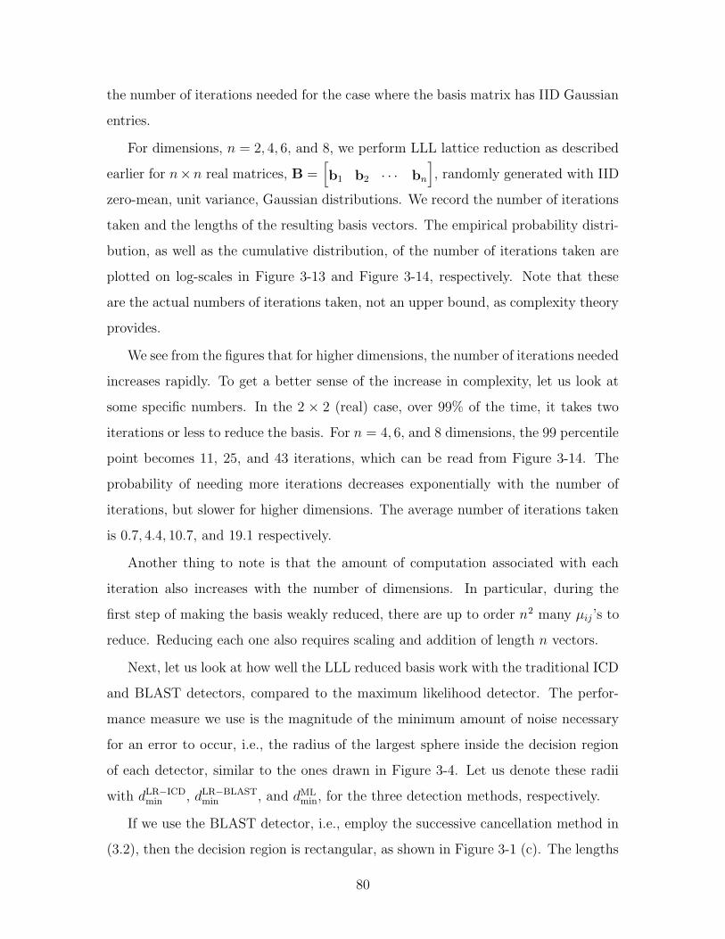
the number of iterations needed for the case where the basis matrix has IID Gaussian
entries.
For dimensions, n = 2, 4, 6, and 8, we perform LLL lattice reduction as described
earlier for n×n real matrices, B =[b1 b2 · · · bn
], randomly generated with IID
zero-mean, unit variance, Gaussian distributions. We record the number of iterations
taken and the lengths of the resulting basis vectors. The empirical probability distri-
bution, as well as the cumulative distribution, of the number of iterations taken are
plotted on log-scales in Figure 3-13 and Figure 3-14, respectively. Note that these
are the actual numbers of iterations taken, not an upper bound, as complexity theory
provides.
We see from the figures that for higher dimensions, the number of iterations needed
increases rapidly. To get a better sense of the increase in complexity, let us look at
some specific numbers. In the 2 × 2 (real) case, over 99% of the time, it takes two
iterations or less to reduce the basis. For n = 4, 6, and 8 dimensions, the 99 percentile
point becomes 11, 25, and 43 iterations, which can be read from Figure 3-14. The
probability of needing more iterations decreases exponentially with the number of
iterations, but slower for higher dimensions. The average number of iterations taken
is 0.7, 4.4, 10.7, and 19.1 respectively.
Another thing to note is that the amount of computation associated with each
iteration also increases with the number of dimensions. In particular, during the
first step of making the basis weakly reduced, there are up to order n2 many µij’s to
reduce. Reducing each one also requires scaling and addition of length n vectors.
Next, let us look at how well the LLL reduced basis work with the traditional ICD
and BLAST detectors, compared to the maximum likelihood detector. The perfor-
mance measure we use is the magnitude of the minimum amount of noise necessary
for an error to occur, i.e., the radius of the largest sphere inside the decision region
of each detector, similar to the ones drawn in Figure 3-4. Let us denote these radii
with dLR−ICDmin , dLR−BLASTmin , and dMLmin, for the three detection methods, respectively.
If we use the BLAST detector, i.e., employ the successive cancellation method in
(3.2), then the decision region is rectangular, as shown in Figure 3-1 (c). The lengths
80
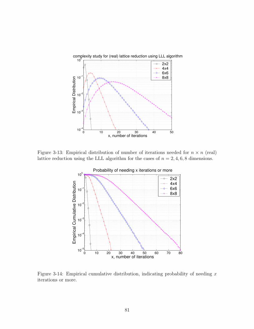
0 10 20 30 40 5010
−4
10−3
10−2
10−1
100
x, number of iterations
Em
piric
al D
istri
butio
n
complexity study for (real) lattice reduction using LLL algorithm
2x24x46x68x8
Figure 3-13: Empirical distribution of number of iterations needed for n × n (real)lattice reduction using the LLL algorithm for the cases of n = 2, 4, 6, 8 dimensions.
0 10 20 30 40 50 60 70 8010
−5
10−4
10−3
10−2
10−1
100
x, number of iterations
Em
piric
al C
umul
ativ
e D
istri
butio
n
Probability of needing x iterations or more
2x24x46x68x8
Figure 3-14: Empirical cumulative distribution, indicating probability of needing xiterations or more.
81
of the sides are ‖bi(i)‖, the component of bi orthogonal to b1, · · · ,bi−1. Instead, wehave dLR−BLASTmin = 1
2mini ‖bi(i)‖. For the ICD detector, we need to look at ‖bi‖, the
component of bi orthogonal to all other vectors, not just the previous ones. Therefore,
dLR−ICDmin = 12mini ‖bi‖. In the case of ML detector, the corresponding measure is the
length of the true shortest vector of the lattice, ξ. We have dMLmin = 1
2ξ. When the
number of dimensions is not too large, the shortest vector of a lattice can be found
using either brute force search or a more efficient technique called sphere decoding
[26, 38].
For dimensions n = 2, 4, 6, and 8, we plot the empirical distribution of the ratio
dLR−BLASTmin /dMLmin and dLR−ICDmin /dML
min for LLL reduced bases in figure Figure 3-15 and
Figure 3-16, respectively.
We see that as the number of dimensions increases, the distribution of the ratio
moves down from 1, meaning that LR-BLAST and LR-ICD become further away from
optimal. The worst case ratio also moves down. After 105 trials, the empirical worst
case found for LR-BLAST is 1.7, 3.3, 4.0, and 6.1 dB from optimal for n = 2, 4, 6, 8
dimensions. For LR-ICD, the gaps are 1.7, 4.3, 6.4, and 8.8 dB. Compared to LR-
ICD, LR-BLAST not only performs better on average, but also seems to have better
worst case bound.
One technical detail to note is the 4/3 factor in (3.14). If we were to use other
values between 4/3 and 1, then we would get better reduced basis at the expense of
increased complexity.
3.8 Summary
In this chapter, we studied uncoded MIMO communication systems and proposed
new coherent detection methods. By incorporating lattice reduction, these methods
significantly improve the performance of traditionally employed low-complexity de-
tectors, in particular, ICD and BLAST detectors. We investigated the case of the
two-transmit two-receive antenna systems in detail. We presented an iterative lattice
reduction algorithm for finding the optimal basis and studied its complexity. We
82

0.6 0.8 10
1000
2000
3000
4000
5000
dminLR−BLAST / d
minML 2x2 case
0.6 0.8 10
1000
2000
3000
4000
5000
dminLR−BLAST / d
minML 4x4 case
0.6 0.8 10
1000
2000
3000
4000
5000
dminLR−BLAST / d
minML 6x6 case
0.6 0.8 10
1000
2000
3000
4000
5000
dminLR−BLAST / d
minML 8x8 case
Figure 3-15: Performance of LR-BLAST detectors using the LLL algorithm, com-pared to that of the ML detector, for n = 2, 4, 6, 8 dimensional cases. The ratiodLR−BLASTmin /dML
min indicates how far LR-BLAST is away from optimal.
0.4 0.6 0.8 10
2000
4000
6000
8000
10000
dminLR−ICD / d
minML 2x2 case
0.4 0.6 0.8 10
2000
4000
6000
8000
10000
dminLR−ICD / d
minML 4x4 case
0.4 0.6 0.8 10
2000
4000
6000
8000
10000
dminLR−ICD / d
minML 6x6 case
0.4 0.6 0.8 10
2000
4000
6000
8000
10000
dminLR−ICD / d
minML 8x8 case
Figure 3-16: Performance of LR-ICD detectors using the LLL algorithm, comparedto that of the ML detector, for n = 2, 4, 6, 8 dimensional cases.
83
showed that the number of iterations needed is typically small and it is increasingly
unlikely to need more. We also showed that, relative to optimal MLD, LR techniques
is sub-optimal by no more than 3 dB in terms of SNR for any Gaussian channel,
and allows us to achieve the same diversity on the Rayleigh fading channel, assuming
sufficiently large constellations are used.
While the proofs and simulations in this study are mostly limited to the 2×2 case,
for higher dimensional cases, lattice reduction ideas can still be applied. However, the
complexity increases, as well as the average and worst-case gap to MLD. So generally
speaking, this lattice reduction idea is mainly meant for applying to low dimensional
cases.
One shortcoming of lattice decoding is that the constellation is treated as an
infinite lattice, so there is a boundary issue. When the received signal falls outside
of the valid constellation region, the nearest lattice point found may not be a valid
codeword. This would lead to errors that could be avoided by MLD.
Extending lattice reduction techniques to transmitter pre-coding can lead to ad-
ditional benefits. In this work, we briefly illustrated the basic ideas graphically; the
details are left for future development. If we were also allowed to transmit at different
rates for each entry of x and the objective were to maximize the total rate, we might
also want to employing water-filling techniques.
84
Chapter 4
Structured Codes with Minimum
Delay
4.1 Introduction
In this chapter, we investigate the problem of using short structured space-time block
codes to achieve the optimal diversity-multiplexing tradeoff in the case of two-transmit
two-receive antenna systems, and try to understand what is fundamentally possible.
For this case, the optimal tradeoff was examined in section 2.3.3 and plotted in
Figure 2-4.
The primary question of interest here is whether the optimal tradeoff can be
achieved using length-two codes. From the rank criterion in Lemma 2.3 in section 2.4,
we see that it is necessary to have T ≥ Nt = 2 to achieve full diversity. In section 2.5,
we see that Gaussian random codes with code length T ≥ 3 can achieve the optimal
tradeoff, while those with T = 2 can not. In this chapter, we answer this previously
open question by presenting a length-two code which we call tilted-QAM code that
can in fact achieve the optimal tradeoff.
The system model we use in this chapter is Y = HX+W, where X is the 2× 2
transmitted signal matrix, H is the 2 × 2 channel matrix, W is the additive white
Gaussian noise and Y is the received signal. Under the Rayleigh fading model, the
entries of H are independent and identically distributed CN(0, 1) random variables,
85
and are assumed to be known by the receiver, but not the transmitter.
We first review a well-known length-two code called the orthogonal space time
block code in section 4.2. OSTBC is a well structured code and is highly attractive
for its low decoding complexity. It uses a smart repetition to ensure all its difference
matrices are full rank, thus achieving the maximum diversity gain. However, this
repetition causes a loss of multiplexing gain. The tradeoff it achieves is below that of
the length-two Gaussian random code.
In the rest of this chapter, we develop the tilted-QAM coding scheme. In sec-
tion 4.3, we introduce the design of the tilted-QAM code, which improves upon
OSTBC by replacing the repetition with a suitably chosen rotation. 1 Using the
criterion of maximizing the worst case determinant, we identify a set of rotation an-
gles that is universally optimal and leads to the same worst case determinant for
all rates. In section 4.4, we analyze the performance of the tilted-QAM code from
two perspectives, and show that our design can indeed achieve the optimal diversity-
multiplexing tradeoff. We believe that having the worst case determinant maintaining
a non-vanishing distance away from zero as rate increases is important for obtaining
the optimal tradeoff. In section 4.5, we numerically simulate the performance of the
tilted-QAM code to demonstrate that the optimal tradeoff is effectively achieved. In
section 4.6, we discuss applying the tilted-QAM code design idea to a single antenna
fading problem.
4.2 OSTBC
An existing well-known space-time code is OSTBC, first introduced by Alamouti in
[1] for the two transmit and any number of receive antennas case, and then extended
by Tarokh in [34] for more general cases. In this section, we first describe the smart
repetition structure of OSTBC and then evaluate the diversity-multiplexing tradeoff
achieved. We also present numerical simulation results at the end.
1Interestingly, such rotation ideas are also used by Boutros and Viterbo [3] in their design ofcodes for single antenna fading channels.
86
4.2.1 The Smart Repetition
OSTBC encodes two information symbols, s1 and s2, into one 2×2 transmitted signal
matrix X in the following fashion,
X =
s1 −s∗2s2 s∗1
, (4.1)
where, (·)∗ indicates conjugation. We see that it effectively transmits each of the two
symbols twice, using two antennas in two time slots.
The resulting received signal is
y11 y12
y21 y22
=
h11 h12
h21 h22
s1 −s∗2s2 s∗1
+
w11 w12
w21 w22
. (4.2)
We can rearrange terms and conjugate y12 and y22 to obtain the effective channel
y11
y21
y∗12
y∗22
=
h11 h12
h21 h22
h∗12 −h∗11h∗22 −h∗21
s1
s2
+
w11
w21
w∗12
w∗22
. (4.3)
The effective channel vectors,[h11 h21 h∗12 h∗22
]Tand
[h12 h22 −h∗11 −h∗21
]T, are
orthogonal to each other. Therefore, there is no interference between s1 and s2.
Component-wise decoding can be easily done. Low complexity is one of the major
advantages of OSTBC.
4.2.2 Theoretical Performance Analysis
In this section, we examine the diversity-multiplexing tradeoff achieved by OSTBC.
By using repetition to spread each symbol across space and time, OSTBC can
achieve the maximum diversity. This can be shown using Lemma 2.3, according to
which, we need to verify that all difference matrices are full rank, i.e., have non-zero
87
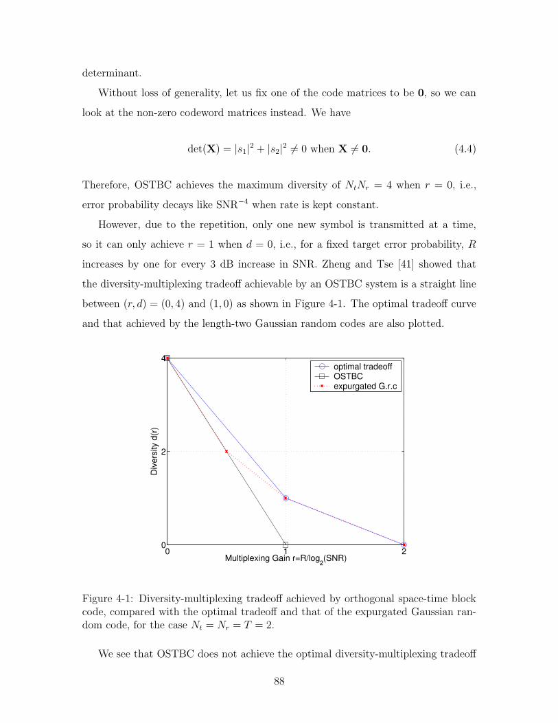
determinant.
Without loss of generality, let us fix one of the code matrices to be 0, so we can
look at the non-zero codeword matrices instead. We have
det(X) = |s1|2 + |s2|2 6= 0 when X 6= 0. (4.4)
Therefore, OSTBC achieves the maximum diversity of NtNr = 4 when r = 0, i.e.,
error probability decays like SNR−4 when rate is kept constant.
However, due to the repetition, only one new symbol is transmitted at a time,
so it can only achieve r = 1 when d = 0, i.e., for a fixed target error probability, R
increases by one for every 3 dB increase in SNR. Zheng and Tse [41] showed that
the diversity-multiplexing tradeoff achievable by an OSTBC system is a straight line
between (r, d) = (0, 4) and (1, 0) as shown in Figure 4-1. The optimal tradeoff curve
and that achieved by the length-two Gaussian random codes are also plotted.
0 1 20
2
4
Multiplexing Gain r=R/log2(SNR)
Div
ersi
ty d
(r)
optimal tradeoffOSTBCexpurgated G.r.c
Figure 4-1: Diversity-multiplexing tradeoff achieved by orthogonal space-time blockcode, compared with the optimal tradeoff and that of the expurgated Gaussian ran-dom code, for the case Nt = Nr = T = 2.
We see that OSTBC does not achieve the optimal diversity-multiplexing tradeoff
88
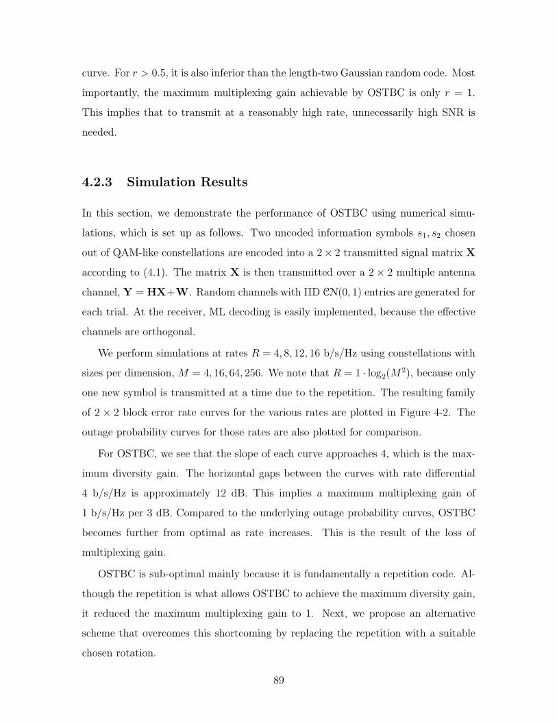
curve. For r > 0.5, it is also inferior than the length-two Gaussian random code. Most
importantly, the maximum multiplexing gain achievable by OSTBC is only r = 1.
This implies that to transmit at a reasonably high rate, unnecessarily high SNR is
needed.
4.2.3 Simulation Results
In this section, we demonstrate the performance of OSTBC using numerical simu-
lations, which is set up as follows. Two uncoded information symbols s1, s2 chosen
out of QAM-like constellations are encoded into a 2× 2 transmitted signal matrix X
according to (4.1). The matrix X is then transmitted over a 2× 2 multiple antenna
channel, Y = HX+W. Random channels with IID CN(0, 1) entries are generated for
each trial. At the receiver, ML decoding is easily implemented, because the effective
channels are orthogonal.
We perform simulations at rates R = 4, 8, 12, 16 b/s/Hz using constellations with
sizes per dimension, M = 4, 16, 64, 256. We note that R = 1 · log2(M2), because only
one new symbol is transmitted at a time due to the repetition. The resulting family
of 2 × 2 block error rate curves for the various rates are plotted in Figure 4-2. The
outage probability curves for those rates are also plotted for comparison.
For OSTBC, we see that the slope of each curve approaches 4, which is the max-
imum diversity gain. The horizontal gaps between the curves with rate differential
4 b/s/Hz is approximately 12 dB. This implies a maximum multiplexing gain of
1 b/s/Hz per 3 dB. Compared to the underlying outage probability curves, OSTBC
becomes further from optimal as rate increases. This is the result of the loss of
multiplexing gain.
OSTBC is sub-optimal mainly because it is fundamentally a repetition code. Al-
though the repetition is what allows OSTBC to achieve the maximum diversity gain,
it reduced the maximum multiplexing gain to 1. Next, we propose an alternative
scheme that overcomes this shortcoming by replacing the repetition with a suitable
chosen rotation.
89

0 10 20 30 40 50 60
10−5
10−4
10−3
10−2
10−1
100
(total) SNR in dB
(2x2
) Blo
ck E
rror
Rat
e
OSTBC, Nt=N
r=2, M=2[2:2:8], Rate=[4:4:16] bits/sec/Hz
<−−−12dB−−−>M=4, R=4M=16, R=8M=64, R=12M=256, R=16
Figure 4-2: Error rate curves of OSTBC (dark) and outage probability curves (light)for various rates. We see that the maximum diversity of four is achieved, but thereis a loss of multiplexing gain.
4.3 Tilted-QAM Code
4.3.1 The Rotation Design
In the OSTBC design we studied in the last section, the key feature allowing it to
achieve full diversity is that both information symbols s1 and s2 appear in both rows
and columns of the codeword matrix X via repetition. However, the simple repetition
causes a loss of multiplexing gain. In a 2×2 codeword matrix, which has four entries,
there are effectively only two information symbols.
We propose a new design named tilted-QAM, which replaces the repetition in OS-
TBC with a suitably chosen rotation. For a given transmission rate R = r log2(SNR),
we use a M 2-QAM constellation carved from Z + Zj with size M 2 = 2R/2 = SNRr/2.
Then, four information symbols, sij, instead of two, are encoded into a codeword
90
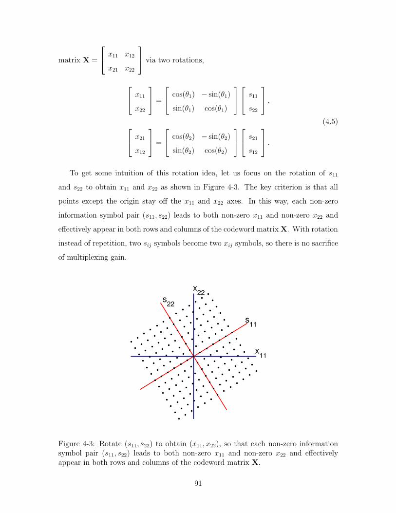
matrix X =
x11 x12
x21 x22
via two rotations,
x11
x22
=
cos(θ1) − sin(θ1)
sin(θ1) cos(θ1)
s11
s22
,
x21
x12
=
cos(θ2) − sin(θ2)
sin(θ2) cos(θ2)
s21
s12
.
(4.5)
To get some intuition of this rotation idea, let us focus on the rotation of s11
and s22 to obtain x11 and x22 as shown in Figure 4-3. The key criterion is that all
points except the origin stay off the x11 and x22 axes. In this way, each non-zero
information symbol pair (s11, s22) leads to both non-zero x11 and non-zero x22 and
effectively appear in both rows and columns of the codeword matrixX. With rotation
instead of repetition, two sij symbols become two xij symbols, so there is no sacrifice
of multiplexing gain.
x11
x22
s11
s22
Figure 4-3: Rotate (s11, s22) to obtain (x11, x22), so that each non-zero informationsymbol pair (s11, s22) leads to both non-zero x11 and non-zero x22 and effectivelyappear in both rows and columns of the codeword matrix X.
91

One thing to note is that although it is possible to choose the rotation angle θ1
so that all points except the origin stay off the axes as shown in Figure 4-3, it is not
possible to keep them a constant distance away from the axes as the constellation
grows. This is because if we project such a two-dimensional lattice on to the x11-
axis, it can be shown that the resulting set of points must be dense on the axis.
Therefore, there must be points with x11 (and similarly x22) arbitrarily close to zero.
Interestingly, it turns out that the product x11x22 can be kept a constant distance
away from zero, which eventually leads to a certain minimum determinant. In the
case of OSTBC, there is essentially a one dimensional lattice along the x11 = ±x22direction, and x11 and x22 are both kept away from zero by a fixed amount. This is
sufficient for having a certain minimum determinant but not necessary.
4.3.2 Choice of rotation angles
In this section, using the criterion of maximizing the worst case determinant, we
identify a set of rotation angles that is universally optimal and leads to the same
worst case determinant for all rates.
While the rotation avoids the multiplexing gain penalty, to ensure maximum di-
versity (when r = 0), we must make all non-zero codeword matrices (equivalent to
all difference matrices) full rank. A slightly stronger condition is to maximize the
worst case determinant, as discussed in section 2.4. Let the worst case determinant
be γdef= minX6=0 | det(X)|. We need to choose the two rotation angles to maximize γ.
Let us first look at det(X) as a function of (θ1, θ2).
2 det(X) = sin(2θ1)(s211−s222) + 2 cos(2θ1)s11s22 (4.6)
− sin(2θ2)(s221−s212)− 2 cos(2θ2)s12s21.
In the case of binary constellation, sij each take the value of 0 and 1, so there are
only 24 − 1 = 15 non-trivial 4-tuples. Since sin and cos are both smooth functions,
we can easily analytically solve for or search for the best pairs of (2θ1, 2θ2) that
maximize γ. To demonstrate this visually, we sweep 2θ1 and 2θ2 each from 0 to π
92
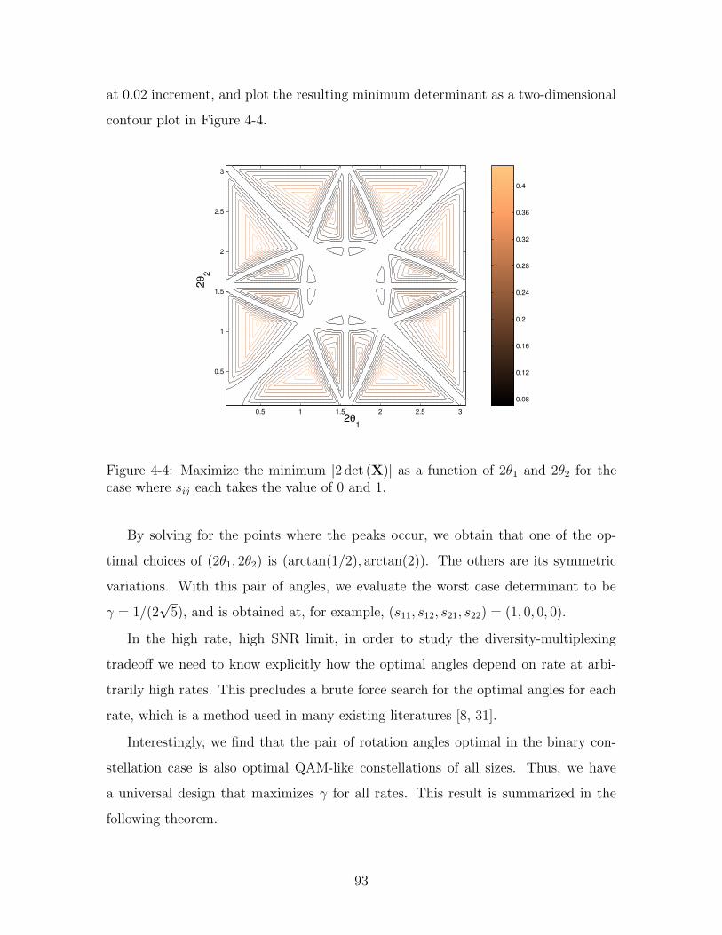
at 0.02 increment, and plot the resulting minimum determinant as a two-dimensional
contour plot in Figure 4-4.
0.5 1 1.5 2 2.5 3
0.5
1
1.5
2
2.5
3
2θ1
2
θ 2
0.08
0.12
0.16
0.2
0.24
0.28
0.32
0.36
0.4
Figure 4-4: Maximize the minimum |2 det (X)| as a function of 2θ1 and 2θ2 for thecase where sij each takes the value of 0 and 1.
By solving for the points where the peaks occur, we obtain that one of the op-
timal choices of (2θ1, 2θ2) is (arctan(1/2), arctan(2)). The others are its symmetric
variations. With this pair of angles, we evaluate the worst case determinant to be
γ = 1/(2√5), and is obtained at, for example, (s11, s12, s21, s22) = (1, 0, 0, 0).
In the high rate, high SNR limit, in order to study the diversity-multiplexing
tradeoff we need to know explicitly how the optimal angles depend on rate at arbi-
trarily high rates. This precludes a brute force search for the optimal angles for each
rate, which is a method used in many existing literatures [8, 31].
Interestingly, we find that the pair of rotation angles optimal in the binary con-
stellation case is also optimal QAM-like constellations of all sizes. Thus, we have
a universal design that maximizes γ for all rates. This result is summarized in the
following theorem.
93

Theorem 1 For codeword matrix X defined in (4.5), the maximum worst case de-
terminant of difference matrices is
max(θ1,θ2)
minX1 6=X2
| det(X1 −X2)| =1
2√5, (4.7)
and achieved by (θ1, θ2)=(12arctan(1
2), 1
2arctan(2)
)for QAM-like constellations of all
sizes.
Proof:
For binary constellation, by listing all det(X) expressions for all sij 4-tuples, we showed
that (θ1, θ2) and its symmetric variations are optimal, with which γ = 1/(2√5) and is
obtained at, for example, (s11, s12, s21, s22) = (1, 0, 0, 0). As constellation grows, γ can onlydecrease or remain constant, since there are additional codewords to minimize over. Soto prove Theorem 1, it suffices to show that γ = 1/(2
√5) is actually achievable for larger
constellations using (θ1, θ2), i.e., | det(X)|≥1/(2√5) for all non-zero 4-tuples of sij ∈ Z+Zj.
Substituting (θ1, θ2) into (4.6), we have,
Jdef= 2√5 det(X) = s211 − s222 + 4s11s22 + 2s
212 − 2s221 − 2s21s12. (4.8)
Since sij ∈ Z+ Zj, so is J . Now we need to prove the following.
Lemma 4.1 For sij ∈ Z + Zj, J = s211 − s222 + 4s11s22 + 2s212 − 2s221 − 2s21s12 = 0 if and
only if s11 = s12 = s21 = s22 = 0.
Let us perform completion of squares and change of variables. Let adef= s11 + 2s22, b
def= s22,
cdef= 2s12 − s21, and d
def= s21, then 2J = 2a
2 − 10b2 + c2 − 5d2. Now we need to prove2a2 + c2 = 5(2b2 + d2) only when a = b = c = d = 0, which requires the following lemma.
Lemma 4.2 For x, y ∈ Z+ Zj, if 5|2x2 + y2, then 5|x, 5|y, and 25|2x2 + y2. 2
Proof:Let x = 5qx + rx and y = 5qy + ry, such that, rx, ry ∈ 0, 1, 2, 3, 4+ 0, 1, 2, 3, 4j andqx, qy ∈ Z+ Zj. 5|2x2 + y2 implies 5|2r2x + r2y. It is straight forward to verify that the onlycase where 5|2r2x + r2y is rx = ry = 0. Therefore, 5|x, 5|y, and 25|2x2 + y2.Now using Lemma 4.2, we can show that
2a2 + c2 = 5(2b2 + d2
)(4.9)
⇒ 5|2a2 + c2 ⇒ 5|a, 5|c, 25|2a2 + c2
⇒ 5|2b2 + d2 ⇒ 5|b, 5|d, 25|2b2 + d2
2For complex integers, divisibility by a real integer (denoted by |) is defined as both real andimaginary parts being divisible.
94
Since all a, b, c, and d are divisible by 5, we can divide both sides of (4.9) by 52 and obtain
an essentially identical equation, 2a′2+ c′2 = 5(2b′2 + d′2
), where a′, b′, c′, d′ ∈ Z+ Zj. We
can repeat the above argument and divide both sides by 52 indefinitely. Thus, the onlypossible solution is a = b = c = d = 0, i.e., s11 = s12 = s21 = s22 = 0. This concludes theproof of Lemma 4.1 and Theorem 1.
One follow-up question is how sensitive the worst case determinant is to the values
of θ1 and θ2. From Figure 4-4, we can see the sensitivity in the case of binary
constellation. For larger constellations, the sensitivity in θ1 and θ2 increases. This
is because for larger constellations, a small change in rotation angle can cause the
points at the edge of the constellation to move by a larger amount.
We numerically demonstrate this effect. To simplify the computation, θ1 is swept
from 0 to π/8, while θ2 = π/4− θ1. We plot the worst case determinant as a function
of θ1 for 2-PAM, 3-PAM, 4-PAM, and 5-PAM constellations in Figure 4-5. We can
clearly see that the sensitivity of the worst case determinant in terms of θ1 increases as
constellation gets larger. While the peak is always at θ1 = arctan(1/2)/2 = 0.23182,
it gets sharper and sharper. Although the sensitivity increases with constellation size,
for practical constellation sizes like 16-QAM or 64-QAM, the numerical accuracy of
the current computers should be sufficient.
4.4 Theoretical Performance Analysis
In this section, we analyze the performance of the tilted-QAM code we proposed
in the last section. The key property of the tilted-QAM code is that the worst case
determinant remains constant as constellation size and rate grows. We show that this
determinant property built into the code allows it to achieve the optimal diversity-
multiplexing tradeoff for two-transmit two-receive antenna systems.
To evaluate the average error probability of the system, we need to average over
both the random channel and the ensemble of codewords. In the next two sections, we
present two perspectives. The first one focuses on the error probability of a particular
channel averaged over all codewords. We show that when the channel is not in outage,
our system tends to have large distances between the received codewords, and thus,
95

0 0.1 0.2 0.3 0.40
0.05
0.1
0.15
0.2
0.25
θ1
wor
st c
ase
dete
rmin
ant
2−PAM constellation
0 0.1 0.2 0.3 0.40
0.05
0.1
0.15
0.2
0.25
θ1
wor
st c
ase
dete
rmin
ant
3−PAM constellation
0 0.1 0.2 0.3 0.40
0.05
0.1
0.15
0.2
0.25
θ1
wor
st c
ase
dete
rmin
ant
4−PAM constellation
0 0.1 0.2 0.3 0.40
0.05
0.1
0.15
0.2
0.25
θ1
wor
st c
ase
dete
rmin
ant
5−PAM constellation
Figure 4-5: Worst-case determinant as a function of θ1, while θ2 = π/4 − θ1. Asconstellation size increases, although the optimal value of θ1 remains at arctan(1/2)/2,the sensitivity increases. Slight deviation of θ1 from its optimal value significantlyreduces the resulting worst-case determinant.
good performance. The second one first looks at the error probability associated with
a particular pair of codewords averaged over all channels, and then sums over the
codewords. This perspective allows us to see that the codeword pairs whose differences
have small determinants are bad and dominate the overall error probability. Thus,
having good determinant property is essential for good performance. We also extend
the second perspective to higher dimensional cases in section 4.4.3.
Before the detailed error probability evaluation, let us first express several key
parameters as functions of SNR in exponential forms. We need to know how they
grow or decay with SNR as SNR grows, because we want to evaluate diversity and
multiplexing gains, which are how fast error probability decays and rate grows with
SNR.
First of all, we chosen to restrict sij ∈ Z+Zj. This means that as SNR increases
and the constellation size grows, the separation between the QAM constellation points
remains at unity.
96
WithM denoting the constellation size per dimension, the average transmit energy
per dimension Es grows with M ,
Es·= M2 = 2R/2 = SNRr/2. (4.10)
The noise level can be expressed as 3
σ2w·=
Es
SNR·= SNRr/2−1. (4.11)
Let λ1 ≥ λ2 denote the singular values of ∆. Using the determinant property
build into the tilted-QAM code that the worst case determinant is always bounded
away from zero by 1/(2√5), we have the lower bound
λ21λ22 = | det(∆)|2 ≥
(1
2√5
)2·= SNR0. (4.12)
The entries of ∆ are at most order M . Therefore, we also have an upper bound
λ21 + λ22 = ‖∆‖2·≤ M2 ·
= SNRr/2. (4.13)
Combining the upper and lower bounds, and using λ1 ≥ λ2, we have:
SNR0·≤ λ21
·≤ SNRr/2 (4.14)
SNR−r/2·≤ λ22
·≤ SNRr/2. (4.15)
These describe how the singular values of ∆ change with SNR.
4.4.1 Minimum Distance Property
In this section, we evaluate the performance of the tilted-QAM design by studying the
minimum distance between received constellation points given a particular channel
3When at the maximum multiplexing gain (r = 2), noise variance is fixed. Since the separationbetween the constellation points is also fixed, the performance remains approximately constant, i.e.,d = 0.
97
realization. For a given H, the distance between a pair of codewords with difference
matrix ∆ is ‖H∆‖, where the norm ‖ · ‖ is defined as ‖A‖2 =∑i,j ‖aij‖2. If ‖H∆‖is at least a certain value, δ(H), for all ∆ 6= 0, then all the received constellation
points are at least distance δ apart. For a given δ, a minimum distance decoder can
guarantee to decode correctly when the magnitude of the noise is less than δ/2.
To show that the optimal tradeoff can be achieved, we first identify δ(H) as a
function of | det(H)| and ‖H‖2. We then relate two expressions, the ratio of δ(H)
to the noise level, δ2(H)/σ2w, and the ratio of the realized channel capacity to rate,
2C(H)/2R. We show that when the channel is not in outage, our system tends to have
large distances between codewords and good performance. Finally, we compare the
conditional error probability P [error|H] achieved by our code to that of the Gaus-
sian random code and conclude that the tilted-QAM code can achieve the optimal
diversity-multiplexing tradeoff.
To lower bound ‖H∆‖2 using | det(H)|, we use the minimum determinant prop-
erty.
‖H∆‖2 ≥ 2| det(H∆)|·≥ | det(H)|. (4.16)
To lower bound ‖H∆‖2 using ‖H‖2, we note that when multiplied by ∆, H must be
scaled by at least λ2, the smaller singular value of ∆.
‖H∆‖2 ≥ λ22‖H‖2·≥ SNR−r/2‖H‖2. (4.17)
Combine the above two bounds on ‖H∆‖2 and the noise variance expression (4.11),
we can lower bound δ2(H)/σ2w with | det(H)| and ‖H‖2,
τdef=
δ2(H)
σ2w
·≥ max
(SNR1−r/2| det(H)|, SNR1−r‖H‖2
). (4.18)
Let us now relate the channel capacity achieved (2.4) to the quantities | det(H)|
98
and ‖H‖2. Using 2R = SNRr, we can rewrite (2.4) as
2C(H)
2R·=(SNR1−r/2| det(H)|
)2+ SNR1−r‖H‖2. (4.19)
Comparing (4.18) and (4.19), we see that both right hand sides involve | det(H)|and ‖H‖2. When C(H) is large compared to R, one of | det(H)| and ‖H‖2 must be
large. Consequently, δ2(H) is large compared to σ2w. So we have
C(H) > R =⇒ τ =δ2(H)
σ2w
·≥ 1. (4.20)
Therefore, when the channel is not in outage, all codewords are well separated com-
pared to the noise level, and correct decoding can be done with high probability. In
other words, the error probability achievable by tilted-QAM codes is very close to the
channel outage probability. This indicates that the tilted-QAM code should be able
to achieve the optimal diversity-multiplexing tradeoff.
Let us take this argument further by examining the conditional error probability
P [error|H] achieved as a result of having a large τ = δ2(H)/σ2w. We first manipulate
the lower bound of τ into an exponential form in SNR, and then express P [error|H]
in terms of τ .
Let λHi be the ordered singular values of H and let SNR−αi = |λH
i |2, as we did in
section 2.3. Then,
| det(H)| = |λH1 λ
H2 | and ‖H‖2 = |λH
1 |2 + |λH2 |2.
When the channel is not in outage, τ·≥ 1, we also have τ 2
·≥ τ . Equation (4.18)
then becomes,
τ 2·≥ max
(SNR2−r|λH
1 |2|λH2 |2, SNR1−r(|λH
1 |2 + |λH2 |2)
)
·≥ SNR2−r|λH
1 |2|λH2 |2 + SNR1−r(|λH
1 |2 + |λH2 |2) + SNR−r
= SNR−r(SNR|λH1 |2 + 1)(SNR|λH
2 |2 + 1)
·= SNR
∑2i=1(1−αi)
+−r (4.21)
99
Recall that (x)+ denotes max(0, x).
Minimum distance decoders can guarantee to decode correctly as long as the
magnitude of the noise is smaller than half of δ(H), the minimum distance between
codewords. Therefore, from a lower bound on τ = δ2(H)/σ2w, we can derive an upper
bound on the error probability. Using the fact that the noise magnitude ‖W‖2 is a
chi-squared random variable of order 8, we have,
P [error|H] < P
[‖W‖2σ2w
> τ/2
]
·=
∫ ∞
u=τ/2
u3e−udu
·= τ 3e−τ/2, (4.22)
where, τ 2·≥ SNR
∑2i=1(1−αi)
+−r when the channel is not in outage.
Let us compare the P [error|H] achieved to that of the Gaussian random code case.
Zheng and Tse showed in [41] that for a Gaussian random code of length T , when
the channel is not in outage, the conditional error probability is
P (error|H)·≤ SNR−T (
∑(1−αi)
+−r). (4.23)
For T ≥ 3, this bound is exponentially tight.
Let η denote SNR(∑(1−αi)
+−r) for short. Comparing (4.22) and (4.23), in the latter,
P (error|H) decays with η like η−T ; in the former, P (error|H) decays like η3/2e−√η/2.
Exponential decays faster than any polynomial, which means that (4.22) behaves like
(4.23) with T → ∞. Therefore, the tilted-QAM code has similar performance as a
Gaussian random code with infinite code length. Since the latter achieves the optimal
diversity-multiplexing tradeoff, so does the tilted-QAM code.
In summary, by looking at the minimum distance properties of the tilted-QAM
code, we showed that it can achieve the optimal diversity-multiplexing tradeoff. We
note that in order to have this result, we exploit the fact that the worst case deter-
minant remains a constant distance away from zero as rate increases, which is a key
property built into the design.
100
4.4.2 Determinant Counting
We present a different way of evaluating error probability in this section. Earlier,
we looked at the performance associated with particular channels. Here, we first
look at the error probability associated with a particular pair of codewords averaged
over all channels, and then sum over the codewords. While the last method identify
what channels are particularly bad, this method allows us to see what codeword pairs
dominate the overall error probability.
We first upper bound the pair-wise error probability P [X1 → X2] by an exponen-
tial of SNR. This bound is exponentially tight when 0 ≤ r ≤ 1, but is loose when
1 < r ≤ 2, due to dropping of a “1+” term. Specifically, using (2.21), we have
P [X1 → X2]·≤(
Nt∏
i=1
(1 +
λ2iσ2w
))−2·≤(
Nt∏
i=1
(λ2iSNR
1−r/2))−2
·=
1
| det (∆)|4SNR2r−4
(4.24)
The above equation is the pair-wise error probability averaged over channel for a
particular pair of codewords with difference matrix ∆. Notice that the worst kind
of codeword pairs are the ones with the smallest determinant, which is order 1. So
the worst-pair error probability is SNR2r−4. This corresponds to a lower bound on
the overall error probability and an upper bound of d(r) = 4 − 2r on the diversity-
multiplexing tradeoff curve. This is a straight line connecting (0, 4) and (2, 0). Com-
paring to the similar tradeoff curve upper bounds for the Gaussian random codes
plotted in Figure 2-10, our upper bound is above that of the length-two expurgated
Gaussian random code and is the same as the one with T =∞.
In order to obtain the total error probability, we need to use the union bound and
sum over all codeword pairs.
Pe <∑
∆6=0P [X1 → X2]
·= SNR2r−4
∑
∆6=0
1
| det (∆)|4 (4.25)
Recall from (4.8) that 2√5 det(∆) = (s211 − s222 + 4s11s22 + 2s212 − 2s221 + 2s21s12),
101

which is a (complex) integer. Let us now look at how often 2√5 det(∆) takes on
different values. For a constellation of sizeM , the range of the determinant is of order
M2, so there are about M 4 possible complex integer values for 2√5 det(∆). There
are order M 8 different ∆ matrices. So if no value of the determinant is particularly
preferred, then the number of ∆ with a particular determinant should be on the order
of M8/M4 = M4. We can then perform the summation
∑
∆6=0
1
| det(∆)|4·= M4
∑
−M4≤a,b≤M4
(a,b)6=(0,0)
1
|a+ bj|4 < M4∑
−∞<a,b<∞
(a,b)6=(0,0)
1
(a2 + b2)2. (4.26)
It can be shown that∑
−∞<a,b<∞
(a,b)6=(0,0)1
(a2+b2)2is a finite constant by using a continuous
integral as an upper bound. Consider the piece-wise constant function g(x, y) that
takes the value 1(a2+b2)2
in the unit square [a − 0.5, a + 0.5) × [b − 0.5, b + 0.5),
(a, b) 6= (0, 0). The integral of this function in the domain outside of the unit square
around the origin equals the sum we wish to bound. Upper bounding g(x, y) with
100(x2+y2)2
and extending the area of integral to√x2 + y2 > 0.5, we can upper bound
the sum with∫∞0.5
100r42πrdr, which is clearly some constant. The sum can also be
numerically evaluated to be 6.0268.
Having∑
−∞<a,b<∞
(a,b)6=(0,0)1
(a2+b2)2being a constant gives us
∑
∆6=0
1
| det(∆)|4·= M4 ·
= SNRr. (4.27)
This implies that we could have just focus on the M 4 difference matrices with the
smallest determinant and ignore the rest.
Combining (4.25) and (4.27), we have
Pe·= SNR2r−4SNRr ·
= SNR3r−4 (4.28)
This corresponds to a diversity-multiplexing tradeoff of d(r) = 4 − 3r, which agrees
with the optimal tradeoff for 0 ≤ r ≤ 1. This shows that the proposed tilted-QAM
scheme can achieve the optimal diversity-multiplexing tradeoff for 0 ≤ r ≤ 1.
102
We note that the above is not a complete proof because of the step where we argued
that there are about M 4 difference matrices ∆ with a particular determinant. To
argue this tightly, it is necessary and sufficient to prove that for −M ≤ Re(sij) ≤M ,
−M ≤ Im(sij) ≤M , and any J ∈ Z+Zj, (s211−s222+4s11s22+2s212−2s221+2s21s12) = J
has at most order M 4 solutions.
At this point, it is still a conjecture without proof. The argument above simply
seemed reasonable and agrees with our numerical simulations in which the number
of solutions is counted. In our simulation, we count the number of times |J(sij)| = 1,
with sij taking only real values between −M and M instead of complex numbers
to allow ourselves to go to greater M . With real numbers, we expect the number of
solutions to be of orderM 2. We growM exponentially from 4 up to 256 at increments
of around√2. The number of solutions as a function of M is plotted in Figure 4-6 on
a log-log scale so that exponent is revealed as slope. We see that the curve approaches
a straight line as M becomes sufficiently large. A linear fit of the curve from M = 16
to M = 256 shows a slope of 1.97 and another linear fit of the curve from M = 64
to M = 256 shows a slope of 1.99. This numerical evidence shows that the number
of solutions seems to grow like M 2 for the real case (and M 4, for complex). Further
work is still needed to formally establish this result.
Although this determinant counting perspective does not provide a proof for the
optimality of the tilted-QAM code as the minimum-distance perspective did in the
last section, it nevertheless provides an intuition for what contributes the most to
error events and how worst case determinant plays a role. It is interesting to note
that in the tilted-QAM code, there are many worst-case codeword pairs. This could
be interpreted as that the codewords are so carefully placed that they are equally
close to many other codewords in many directions.
4.4.3 Determinant Counting: Higher Dimensional Cases
In the previous sections, we have focused on a multiple antenna system with two-
transmit two-receive antennas. The optimal diversity multiplexing tradeoff curve has
two piece-wise linear segments, between 0 ≤ r ≤ 1 and 1 ≤ r ≤ 2. Generally speaking,
103
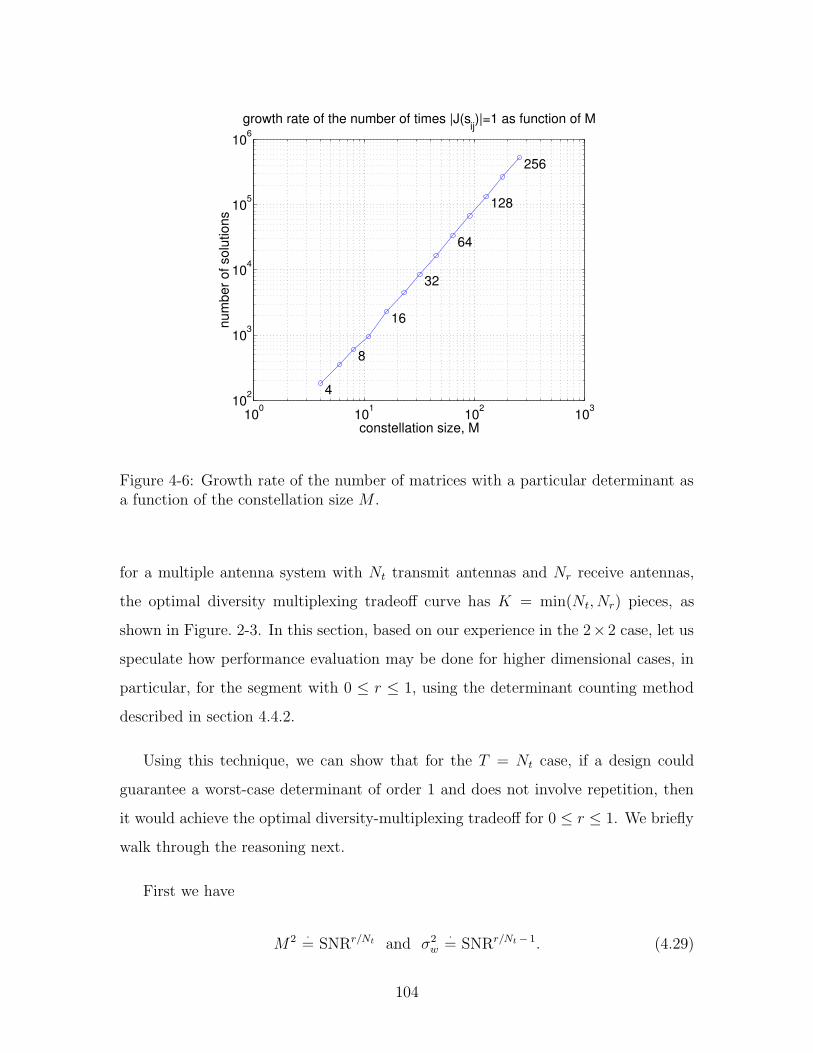
100
101
102
10310
2
103
104
105
106
constellation size, M
num
ber o
f sol
utio
ns
growth rate of the number of times |J(sij)|=1 as function of M
4
8
16
32
64
128
256
Figure 4-6: Growth rate of the number of matrices with a particular determinant asa function of the constellation size M .
for a multiple antenna system with Nt transmit antennas and Nr receive antennas,
the optimal diversity multiplexing tradeoff curve has K = min(Nt, Nr) pieces, as
shown in Figure. 2-3. In this section, based on our experience in the 2× 2 case, let us
speculate how performance evaluation may be done for higher dimensional cases, in
particular, for the segment with 0 ≤ r ≤ 1, using the determinant counting method
described in section 4.4.2.
Using this technique, we can show that for the T = Nt case, if a design could
guarantee a worst-case determinant of order 1 and does not involve repetition, then
it would achieve the optimal diversity-multiplexing tradeoff for 0 ≤ r ≤ 1. We briefly
walk through the reasoning next.
First we have
M2 ·= SNRr/Nt and σ2w
·= SNRr/Nt− 1. (4.29)
104
The pair-wise error probability averaged over all channels is
P [X1 → X2]·≤(
Nt∏
i=1
(1 +
λ2iσ2w
))−Nr
·=
1
| det (∆)|2NrSNRrNr−NtNr (4.30)
The total error probability can be upper bounded using the union bound :
Pe <∑
∆6=0P [X1 → X2]
·= SNRrNr−NtNr
∑
∆6=0
1
| det (∆)|2Nr(4.31)
Again, we need to count the number of times each det(∆) value occurs. There are
M2N2t codewords, and the range of det(∆) is of order MNt . So each determinant
occurs about M 2N2t −2Nt = M2Nt(Nt−1) = SNRr(Nt−1) times. Focusing only on those
with the smallest determinant, the overall error probability is
Pe·= SNRrNr−NtNrSNRr(Nt−1) = SNR−(NtNr−rNr−rNt+1).
Therefore, the diversity-multiplexing tradeoff achieved is d(r) = NtNr−rNr−rNt+1.
Evaluating it at r = 0 and 1, we have d(0) = NtNr and d(1) = (Nt − 1)(Nr − 1).
Therefore, the tradeoff achieved agrees with the optimal tradeoff in Lemma 2.1 for
0 ≤ r ≤ 1.
This tells us that for the T = Nt case, if we could design a codebook without using
repetition and guarantee that the smallest determinant is of order 1, then it would
achieve the optimal diversity-multiplexing tradeoff curve for 0 ≤ r ≤ 1. Also, since
the code takes in N 2t information symbols, like the tilted-QAM design instead of the
OSTBC design, we expect the code to achieve the (Nt, 0) points. (Assume Nr ≥ Nt,
so we are not losing any dimensions.) At this point, it is unclear whether these two
properties are sufficient for achieving all the intermediate tradeoff points. We suspect
that other criteria such as maximizing the minimum of some other functions of ∆,
not just the determinant, might be needed.
105
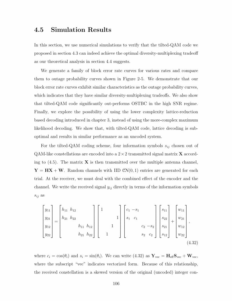
4.5 Simulation Results
In this section, we use numerical simulations to verify that the tilted-QAM code we
proposed in section 4.3 can indeed achieve the optimal diversity-multiplexing tradeoff
as our theoretical analysis in section 4.4 suggests.
We generate a family of block error rate curves for various rates and compare
them to outage probability curves shown in Figure 2-5. We demonstrate that our
block error rate curves exhibit similar characteristics as the outage probability curves,
which indicates that they have similar diversity-multiplexing tradeoffs. We also show
that tilted-QAM code significantly out-performs OSTBC in the high SNR regime.
Finally, we explore the possibility of using the lower complexity lattice-reduction
based decoding introduced in chapter 3, instead of using the more-complex maximum
likelihood decoding. We show that, with tilted-QAM code, lattice decoding is sub-
optimal and results in similar performance as an uncoded system.
For the tilted-QAM coding scheme, four information symbols sij chosen out of
QAM-like constellations are encoded into a 2×2 transmitted signal matrix X accord-
ing to (4.5). The matrix X is then transmitted over the multiple antenna channel,
Y = HX +W. Random channels with IID CN(0, 1) entries are generated for each
trial. At the receiver, we must deal with the combined effect of the encoder and the
channel. We write the received signal yij directly in terms of the information symbols
sij as
y11
y21
y12
y22
=
h11 h12
h21 h22
h11 h12
h21 h22
1
1
1
1
c1 −s1s1 c1
c2 −s2s2 c2
s11
s22
s21
s12
+
w11
w21
w12
w22
,
(4.32)
where ci = cos(θi) and si = sin(θi). We can write (4.32) as Yvec = HeffSvec +Wvec,
where the subscript “vec” indicates vectorized form. Because of this relationship,
the received constellation is a skewed version of the original (uncoded) integer con-
106
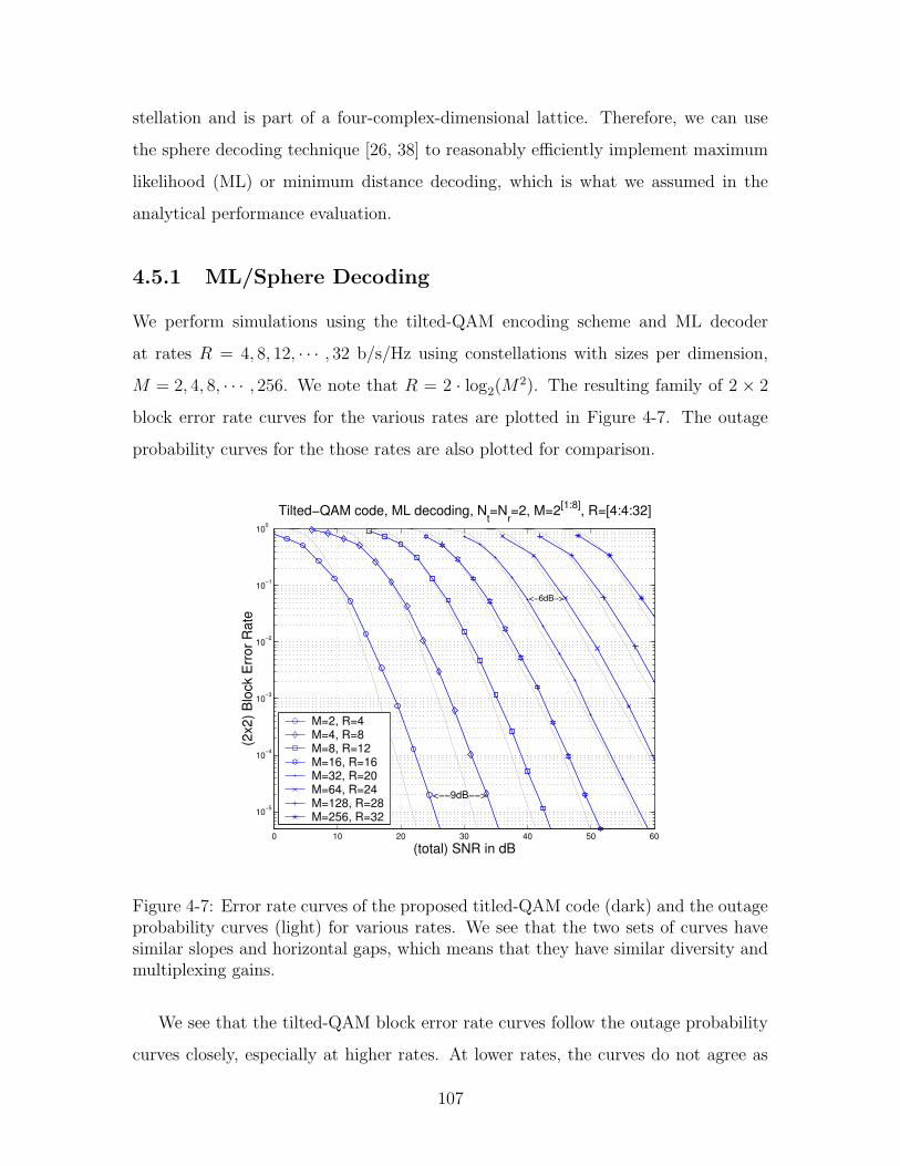
stellation and is part of a four-complex-dimensional lattice. Therefore, we can use
the sphere decoding technique [26, 38] to reasonably efficiently implement maximum
likelihood (ML) or minimum distance decoding, which is what we assumed in the
analytical performance evaluation.
4.5.1 ML/Sphere Decoding
We perform simulations using the tilted-QAM encoding scheme and ML decoder
at rates R = 4, 8, 12, · · · , 32 b/s/Hz using constellations with sizes per dimension,
M = 2, 4, 8, · · · , 256. We note that R = 2 · log2(M2). The resulting family of 2 × 2
block error rate curves for the various rates are plotted in Figure 4-7. The outage
probability curves for the those rates are also plotted for comparison.
0 10 20 30 40 50 60
10−5
10−4
10−3
10−2
10−1
100
(total) SNR in dB
(2x2
) Blo
ck E
rror
Rat
e
Tilted−QAM code, ML decoding, Nt=N
r=2, M=2[1:8], R=[4:4:32]
<−−9dB−−>
<−6dB−>
M=2, R=4M=4, R=8M=8, R=12M=16, R=16M=32, R=20M=64, R=24M=128, R=28M=256, R=32
Figure 4-7: Error rate curves of the proposed titled-QAM code (dark) and the outageprobability curves (light) for various rates. We see that the two sets of curves havesimilar slopes and horizontal gaps, which means that they have similar diversity andmultiplexing gains.
We see that the tilted-QAM block error rate curves follow the outage probability
curves closely, especially at higher rates. At lower rates, the curves do not agree as
107
well. This is because diversity-multiplexing tradeoff is a high SNR characteristic. It
is possible for two systems with the same tradeoff to have different low SNR behavior.
The diversity and multiplexing gains achieved can be measured from the slopes of
the error rate curves and the horizontal spacings between these curves, as discussed
earlier in section 2.3. Let us compare the slopes and gaps achieved by the tilted-QAM
code to that of the linearized outage probability curves show in Figure 2-7. We see
that above the Pout = SNR−1 line, the gaps between the curves with rate differential
4 b/s/Hz is about 6 dB. This implies the maximum multiplexing gain of 2 b/s/Hz per
3 dB. At this location, the slope of the curves is about 2. Below the Pout = SNR−1
line, the slope of each curve approaches 4, which is the maximum diversity gain. The
gaps between the curves is about 9 dB, which corresponds to 4/3 b/s/Hz per 3 dB.
All these slopes and gaps agrees with the optimal tradeoff curve in Figure 2-4.
These simulation results show that the proposed tilted-QAM encoding scheme,
together with ML decoding, can match the outage probability curves and achieve the
optimal diversity-multiplexing tradeoff.
We also note that the diversity-multiplexing tradeoff does not capture constant
factor differences between systems. One system may be a fixed dB inferior than an-
other, while having the same tradeoff. Our simulation results show that the gap
between the tilted-QAM code and the outage probability is in fact quite small,
even though the tilted-QAM code is only designed to achieve the optimal diversity-
multiplexing tradeoff.
Comparing the tilted-QAM code and the OSTBC performance show in Figure 4-2,
we see that at 4 b/s/Hz, they are similar. For rates below 4 b/s/Hz, OSTBC is
near optimal and is preferred for its lower decoding complexity. As rate increases,
tilted-QAM codes out-perform OSTBC by increasing amounts due to the superior
multiplexing gain. Tilted-QAM codes achieve the same rates at much lower SNR;
and since they reach the same limiting slopes, OSTBC never catches up.
108
4.5.2 Lattice Decoding
Earlier in chapter 3, we proposed a lattice-reduction-aided detector that has lower
complexity and achieves near ML performance. One draw back is that this decoder
treats the constellation as an infinite lattice and does not handle constellation bound-
aries.
In this section, we investigate the degree to which this low-complexity decoder
can replace the more-complex ML decoder when the transmitter uses the tilted-QAM
scheme. We show that the maximum diversity can not be achieved due to the bound-
ary problem and the resulting performance is similar to an uncoded system. We first
provide intuition and then present numerical simulation results.
Intuitively, we speculate that due to the boundary issue, the lattice decoder can
not perform as well as the ML decoder. When the constellation boundary is not
considered during decoding, there are effectively many more codeword pairs and many
more difference matrices with small determinant. The determinant counting method
in section 4.4.2 suggests that this can lead to significant performance degradation.
From a different perspective, without the boundary, there is no upper bound on
the energy of the difference matrix ‖∆‖2 as in (4.13). Consequently, there is no lower
bound on the smaller singular value of ∆, λ2, as in (4.15). As a result, there can
never be an SNR large enough so that the (1 + λ22/σ2w) term in the pair-wise error
probability is in effect. Without the contribution from this λ2 term, the slopes of the
error rate curves can only reach 2.
To verify our speculation, we perform simulations with tilted-QAM encoder and
lattice-reduction-aided BLAST decoder at the same constellation sizes and rates as
before. The results are plotted in Figure 4-8. We see that, as we predicted, the slopes
reach a maximum of only 2 and never reach 4. The gaps between the curves are still
6 dB since we do not lose any multiplexing gain.
We notice that Figure 4-8 looks very similar to Figure 3-9, the performance of an
uncoded system with lattice reduction aided detector. This means that when using
lattice decoding, there is no benefit to using the tilted-QAM code. This is because
109
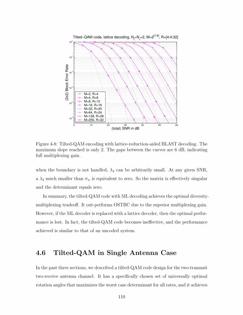
0 10 20 30 40 50 60
10−5
10−4
10−3
10−2
10−1
100
(total) SNR in dB
(2x2
) Blo
ck E
rror
Rat
e
Tilted−QAM code, lattice decoding, Nt=N
r=2, M=2[1:8], R=[4:4:32]
M=2, R=4M=4, R=8M=8, R=12M=16, R=16M=32, R=20M=64, R=24M=128, R=28M=256, R=32
Figure 4-8: Tilted-QAM encoding with lattice-reduction-aided BLAST decoding. Themaximum slope reached is only 2. The gaps between the curves are 6 dB, indicatingfull multiplexing gain.
when the boundary is not handled, λ2 can be arbitrarily small. At any given SNR,
a λ2 much smaller than σw is equivalent to zero. So the matrix is effectively singular
and the determinant equals zero.
In summary, the tilted-QAM code with ML decoding achieves the optimal diversity-
multiplexing tradeoff. It out-performs OSTBC due to the superior multiplexing gain.
However, if the ML decoder is replaced with a lattice decoder, then the optimal perfor-
mance is lost. In fact, the tilted-QAM code becomes ineffective, and the performance
achieved is similar to that of an uncoded system.
4.6 Tilted-QAM in Single Antenna Case
In the past three sections, we described a tilted-QAM code design for the two-transmit
two-receive antenna channel. It has a specifically chosen set of universally optimal
rotation angles that maximizes the worst case determinant for all rates, and it achieves
110
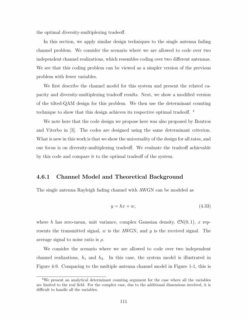
the optimal diversity-multiplexing tradeoff.
In this section, we apply similar design techniques to the single antenna fading
channel problem. We consider the scenario where we are allowed to code over two
independent channel realizations, which resembles coding over two different antennas.
We see that this coding problem can be viewed as a simpler version of the previous
problem with fewer variables.
We first describe the channel model for this system and present the related ca-
pacity and diversity-multiplexing tradeoff results. Next, we show a modified version
of the tilted-QAM design for this problem. We then use the determinant counting
technique to show that this design achieves its respective optimal tradeoff. 4
We note here that the code design we propose here was also proposed by Boutros
and Viterbo in [3]. The codes are designed using the same determinant criterion.
What is new in this work is that we show the universality of the design for all rates, and
our focus is on diversity-multiplexing tradeoff. We evaluate the tradeoff achievable
by this code and compare it to the optimal tradeoff of the system.
4.6.1 Channel Model and Theoretical Background
The single antenna Rayleigh fading channel with AWGN can be modeled as
y = hx+ w, (4.33)
where h has zero-mean, unit variance, complex Gaussian density, CN(0, 1), x rep-
resents the transmitted signal, w is the AWGN, and y is the received signal. The
average signal to noise ratio is ρ.
We consider the scenario where we are allowed to code over two independent
channel realizations, h1 and h2. In this case, the system model is illustrated in
Figure 4-9. Comparing to the multiple antenna channel model in Figure 1-1, this is
4We present an analytical determinant counting argument for the case where all the variablesare limited to the real field. For the complex case, due to the additional dimensions involved, it isdifficult to handle all the variables.
111
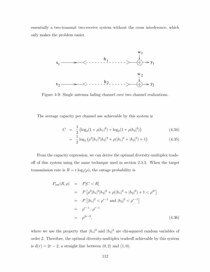
essentially a two-transmit two-receive system without the cross interference, which
only makes the problem easier.
h
h 2
x
x y2
y1
2
1
w
w
1
2
1
Figure 4-9: Single antenna fading channel over two channel realizations.
The average capacity per channel use achievable by this system is
C =1
2
(log2(1 + ρ|h1|2) + log2(1 + ρ|h2|2)
)(4.34)
=1
2log2
(ρ2|h1|2|h2|2 + ρ(|h1|2 + |h2|2) + 1
)(4.35)
From the capacity expression, we can derive the optimal diversity-multiplex trade-
off of this system using the same technique used in section 2.3.3. When the target
transmission rate is R = r log2(ρ), the outage probability is
Pout(R, ρ) = P [C < R]
= P[ρ2|h1|2|h2|2 + ρ(|h1|2 + |h2|2) + 1 < ρ2r
]
·= P
[|h1|2 < ρr−1 and |h2|2 < ρr−1
]
·= ρr−1 · ρr−1
= ρ2r−2, (4.36)
where we use the property that |h1|2 and |h2|2 are chi-squared random variables of
order 2. Therefore, the optimal diversity-multiplex tradeoff achievable by this system
is d(r) = 2r − 2, a straight line between (0, 2) and (1, 0).
112
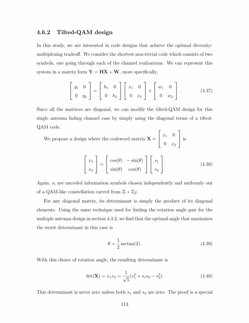
4.6.2 Tilted-QAM design
In this study, we are interested in code designs that achieve the optimal diversity-
multiplexing tradeoff. We consider the shortest non-trivial code which consists of two
symbols, one going through each of the channel realizations. We can represent this
system in a matrix form Y = HX+W, more specifically,
y1 0
0 y2
=
h1 0
0 h2
x1 0
0 x2
+
w1 0
0 w2
. (4.37)
Since all the matrices are diagonal, we can modify the tilted-QAM design for this
single antenna fading channel case by simply using the diagonal terms of a tilted-
QAM code.
We propose a design where the codeword matrix X =
x1 0
0 x2
is
x1
x2
=
cos(θ) − sin(θ)
sin(θ) cos(θ)
s1
s2
. (4.38)
Again, si are uncoded information symbols chosen independently and uniformly out
of a QAM-like constellation carved from Z + Zj.
For any diagonal matrix, its determinant is simply the product of its diagonal
elements. Using the same technique used for finding the rotation angle pair for the
multiple antenna design in section 4.3.2, we find that the optimal angle that maximizes
the worst determinant in this case is
θ =1
2arctan(2). (4.39)
With this choice of rotation angle, the resulting determinant is
det(X) = x1x2 =1√5(s21 + s1s2 − s22). (4.40)
This determinant is never zero unless both s1 and s2 are zero. The proof is a special
113

case of the proof for Lemma 4.1 with just two of the variables, instead of four.
4.6.3 Error Probability Evaluation
Next, let us follow the earlier analysis done for multiple antenna channels and de-
rive error probability expressions for this single antenna channel with the modified
tilted-QAM code design. We again use the determinant counting technique used in
section 4.4.2.
From the error probability expression derived in section 2.4, we have,
P [X1 → X2] ≤ EH
[exp
−‖H∆‖28σ2w
]
= Eh1
[exp
−|h1|2|δ1|28σ2w
]Eh2
[exp
−|h2|2|δ2|28σ2w
]
=1
1 + |δ1|28σ2w
· 1
1 + |δ2|28σ2w
,
where ∆ is the difference codeword matrix with diagonal elements δ1 and δ2.
Mirroring (4.10) and (4.11), we have here,
Es·= M2 = 2R = ρr and σ2w
·=Es
ρ·= ρr−1. (4.41)
Combining the above, we have, similar to (4.24),
P [X1 → X2]·=
1
1 + |δ1|28σ2w
· 1
1 + |δ2|28σ2w
·≤ 1
(|δ1|2|δ2|2)σ4w =
1
| det(∆)|2ρ2r−2. (4.42)
In order to obtain the total error probability, we need to use the union bound and
sum over all codeword pairs, we have, similar to (4.25),
Pe <∑
∆6=0P [X1 → X2]
·= ρ2r−2
∑
∆6=0
1
| det (∆)|2 (4.43)
Now, in order to prove that the optimal tradeoff of d(r) = 2r − 2 is achieved, we
need to show that∑
∆6=01
| det (∆)|2 grows slower than any polynomial power of ρ as
114
rate and constellation size increases.
When all the variables are complex, the summation happens over a four dimen-
sional integer grid, two for each complex diagonal elements of ∆. This summation
is difficult. Instead, let us change the problem and perform this summation for real
variables to develop some intuitions for the complex case.
For the real case, |h1|2 and |h2|2 are chi-squared random variables of order 1,
instead of 2. Because of this, we should sum over 1| det (∆)| instead of 1
| det (∆)|2 .
From the determinant property of the modified tilted-QAM code in (4.40), we
have
| det(∆)| ·= |a2 + ab− b2|, (4.44)
where (a, b), a, b ∈ Z, represents the difference between two information symbol pairs.
When the constellation size is M , the range of a and b is within −M and +M .
Now what we need to evaluate is
∑
∆6=0
1
| det (∆)|·=
∑
−M<a,b<M
(a,b)6=(0,0)
1
|a2 + ab− b2| . (4.45)
In the following lemma, we show that the right hand side quantity grows no faster
than (logM)2. Since M 2 = ρr, this in turn implies that∑
∆6=01
| det (∆)|2·≤(r2log ρ
)2,
which grows slower than any polynomial power of ρ.
Lemma 4.3 For a, b ∈ Z,
∑
−M<a,b<M
(a,b)6=(0,0)
1
|a2 + ab− b2|·≤ (logM)2. (4.46)
Proof:
Let us first divide all the points (a, b) to be summed over into the standard four quadrants.To take care of the axis, let each quadrant include the semi-axis on its clockwise side. Forexample, the first quadrant include all points a ≥ 1, b ≥ 1 and the positive x-axis. Notethat no quadrant contains the origin.
115
Let f(a, b) = |a2 + ab− b2|−1. It has the symmetry property that
f(a, b) = f(−a,−b) = f(b,−a) = f(−b, a). (4.47)
This means that every point in the second, third, and fourth quadrant has a correspondingimage in the first quadrant. Therefore,
∑
−M<a,b<M
(a,b)6=(0,0)
f(a, b) = 4 ·∑
1≤a<M0≤b<M
f(a, b). (4.48)
To sum over the first quadrant, we further divide it into two regions, b > a and a ≥ b.We map points with b > a to points in the a ≥ b region by using the identity
f(a, b) = f(b− a, a). (4.49)
For each point (a, b) with b > a ≥ 1, we map it to (b− a, a). Since b > a to start with,b− a ≥ 1. Therefore, the new point is still inside the first quadrant. We continue with thismapping until we get a point with a ≥ b. For example, starting from (11, 17), we first mapit to (6, 11), then (5, 6), (1, 5), and finally (4, 1), 4 > 1.
All these points, eg., (11, 17), · · · (4, 1), have the same f(a, b) value and they all map tothe same point in the a ≥ b region. We need to count how many points in the b > a regionmap to the same point in the a ≥ b region. We do so by noticing that this sequence ofcoordinates is Fibonacci like, (b− a, a)← (a, (b− a) + a) = (a, b). We know that Fibonacci
number grow exponentially (with limiting rate√5+12 ). Thus, within a certain range M ,
there are logM many such points. Therefore, each point in the a ≥ b region is mapped toby at most order logM points in the b > a region.
Now, we can just sum over the a ≥ b region and multiply the result by logM to takecare of all the points in the b > a region as an upper bound to the total sum.
To sum over the a ≥ b region in the first quadrant, we use an upper bound of f(a, b).When a ≥ b ≥ 0, |a2 + ab− b2| ≥ a2. Thus f(a, b) ≤ 1
a2. Therefore,
∑
1≤a<M0≤b≤a
f(a, b) ≤∑
1≤a<M0≤b≤a
1
a2=
∑
1≤a<M
a+ 1
a2·=
∑
1≤a<M
1
a
·= logM. (4.50)
In summary,
∑
−M<a,b<M
(a,b)6=(0,0)
1
|a2 + ab− b2| = 4∑
1≤a<M0≤b<M
f(a, b)·≤ logM
∑
1≤a<M0≤b≤a
f(a, b)·≤ (logM)2. (4.51)
To numerically verify Lemma 4.3, we plot∑
−M<a,b<M
(a,b)6=(0,0)f(a, b) as a function of M
for M up to 1000 in Figure 4-10. We also plot the curve 5(logM)2 on top of it. We
see that the sum seems to grow a little slower than 5(logM)2.
We also plot the number of times where f(a, b) = 1, which is a significant part
116

0 200 400 600 800 10000
50
100
150
200
250
M, constellation size per dimension
sum(f(a,b))
number of times f(a,b)=1
∝ log(M)2
∝ log(M)
Figure 4-10: The sum∑
−M<a,b<M
(a,b)6=(0,0)f(a, b) as a function of M , the number of times
f(a, b) = 1, and their approximations (dash).
in the total sum. We see that it grows like logM . We can in fact list all of the
solutions. They are the symmetric variations (in the four quadrants) of the point
(1, 0), (1, 1), (1, 2), (2, 3), (3, 5), · · · , the well-known Fibonacci sequence.
4.7 Summary
In this chapter, we studied the problem of designing structured deterministic codes
that achieve the optimal diversity-multiplexing tradeoff. In particular, we focused
on the two-transmit two-receive antennas case, and length two codes, the minimum
needed to achieve the optimal tradeoff. We reviewed the well-known OSTBC code,
which uses a smart repetition to achieve the maximum diversity gain. In doing so, it
sacrifices multiplexing gain.
Realizing the problem of OSTBC, we proposed a tilted-QAM coding design which
replaces the repetition with a suitably chosen rotation while keeping the cross diagonal
structure. Based on the criterion of maximizing the worst case determinant, a set of
rotation angles is identified and proven to be universally optimal for all rate. This
117
universal characterization of the code allows us to analyze its performance in the
high SNR regime. It is then shown that the proposed tilted-QAM design achieves
the optimal diversity-multiplexing tradeoff through both theoretical analysis as well
as numerical simulations.
Prior to this work, there is no known scheme that achieves the optimal diversity-
multiplexing tradeoff for the Nt = Nr = T = 2 case. After Zheng and Tse showed
that Gaussian random code is sub-optimal in this case, it was left as an open question
whether the optimal tradeoff is even achievable at this length. This question is now
answered by our work.
The key to our design is the identification of the rotation angles which guarantees
that the worst case determinants remain a constant distance away from zero as rate
increases.
Comparing tilted-QAM code and OSTBC, similar performance is achieved at
4 b/s/Hz. Above that, tilted-QAM out-performs OSTBC by increasing amounts.
At lower rates, OSTBC is preferred for its lower complexity.
118
Chapter 5
Error Correction Code Enhanced
Systems
5.1 Introduction
In the previous chapter we studied coding for a two-transmit two-receive antenna
system with a length two code that can effectively achieve the optimal diversity-
multiplexing tradeoff. In this chapter we further investigate the role of using longer,
more powerful, error correction codes. The goal is to understand how to build prac-
tical systems with good performance.
In communication systems, it is a common practice to introduce redundancy into
the transmitted signal via coding to improve performance. Error correction coding
for AWGN channels has long been studied. There are well-known soft-decision codes
like the turbo codes and LDPC codes that can approach capacity to within a small
fraction of a dB. There are also hard-decision codes like Reed-Solomon codes, that
have been used in industry for decades.
These codes typically provide coding gains that are measured in terms of constant
gains in SNR in dB. This is different from coding for diversity-multiplexing tradeoff
for multiple antenna channels, which is about the slopes at which probability of error
decays or data rate increases with SNR, rather than constant offsets. Therefore,
we must use long error correction code in addition to codes specifically designed for
119
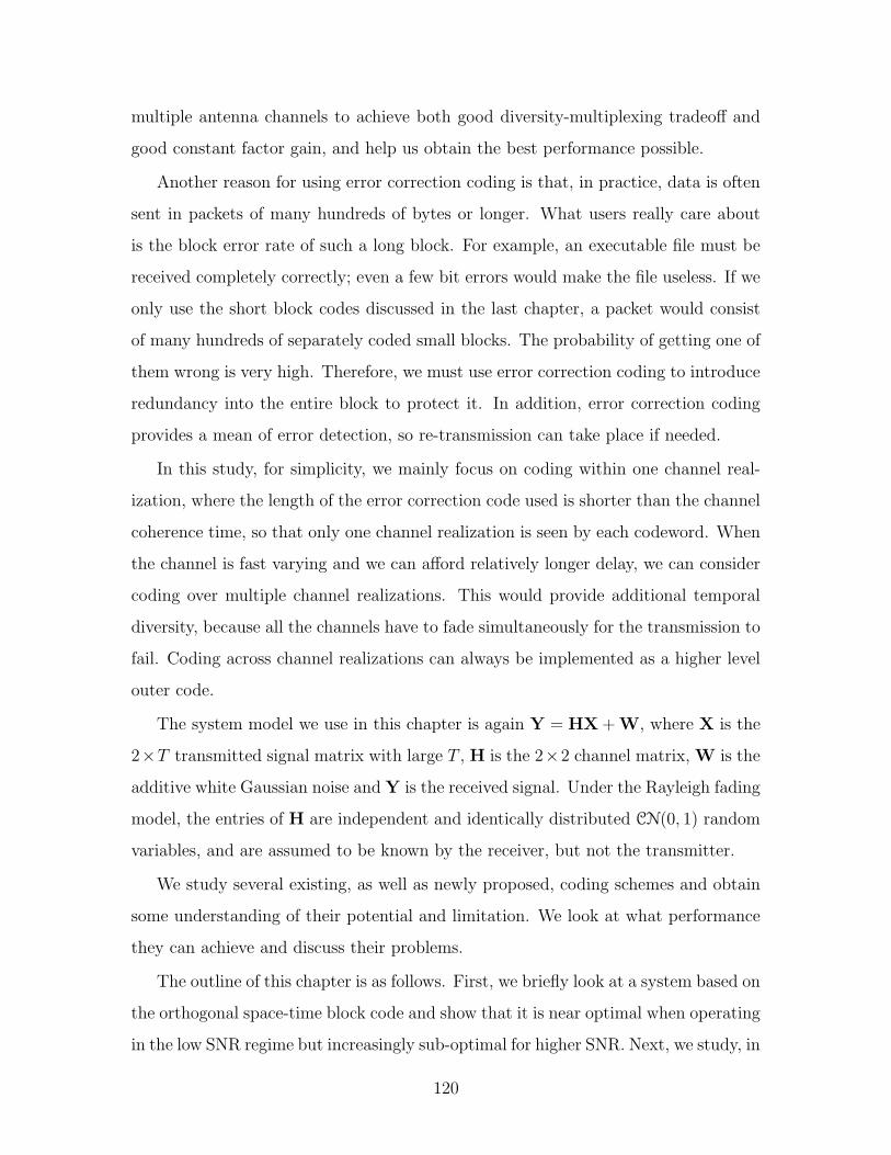
multiple antenna channels to achieve both good diversity-multiplexing tradeoff and
good constant factor gain, and help us obtain the best performance possible.
Another reason for using error correction coding is that, in practice, data is often
sent in packets of many hundreds of bytes or longer. What users really care about
is the block error rate of such a long block. For example, an executable file must be
received completely correctly; even a few bit errors would make the file useless. If we
only use the short block codes discussed in the last chapter, a packet would consist
of many hundreds of separately coded small blocks. The probability of getting one of
them wrong is very high. Therefore, we must use error correction coding to introduce
redundancy into the entire block to protect it. In addition, error correction coding
provides a mean of error detection, so re-transmission can take place if needed.
In this study, for simplicity, we mainly focus on coding within one channel real-
ization, where the length of the error correction code used is shorter than the channel
coherence time, so that only one channel realization is seen by each codeword. When
the channel is fast varying and we can afford relatively longer delay, we can consider
coding over multiple channel realizations. This would provide additional temporal
diversity, because all the channels have to fade simultaneously for the transmission to
fail. Coding across channel realizations can always be implemented as a higher level
outer code.
The system model we use in this chapter is again Y = HX+W, where X is the
2×T transmitted signal matrix with large T , H is the 2×2 channel matrix,W is the
additive white Gaussian noise andY is the received signal. Under the Rayleigh fading
model, the entries of H are independent and identically distributed CN(0, 1) random
variables, and are assumed to be known by the receiver, but not the transmitter.
We study several existing, as well as newly proposed, coding schemes and obtain
some understanding of their potential and limitation. We look at what performance
they can achieve and discuss their problems.
The outline of this chapter is as follows. First, we briefly look at a system based on
the orthogonal space-time block code and show that it is near optimal when operating
in the low SNR regime but increasingly sub-optimal for higher SNR. Next, we study, in
120
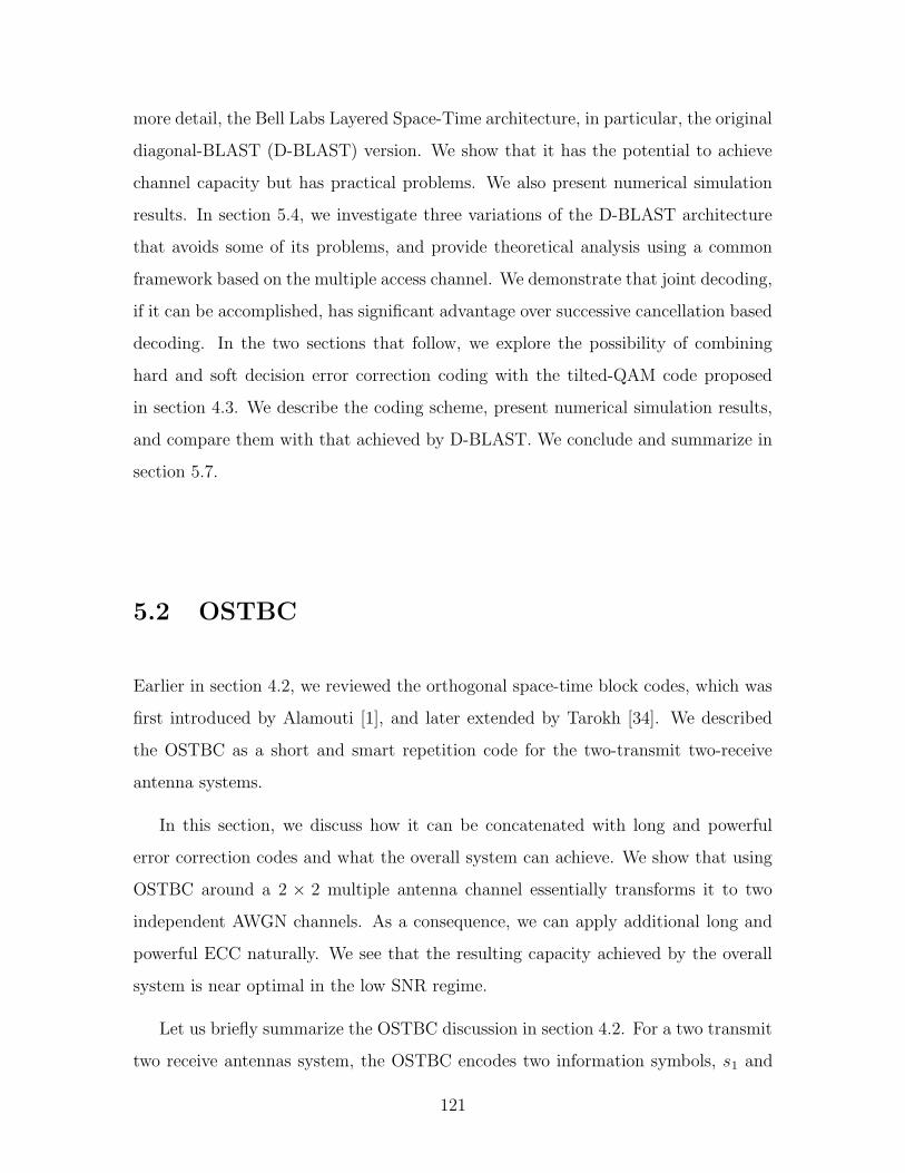
more detail, the Bell Labs Layered Space-Time architecture, in particular, the original
diagonal-BLAST (D-BLAST) version. We show that it has the potential to achieve
channel capacity but has practical problems. We also present numerical simulation
results. In section 5.4, we investigate three variations of the D-BLAST architecture
that avoids some of its problems, and provide theoretical analysis using a common
framework based on the multiple access channel. We demonstrate that joint decoding,
if it can be accomplished, has significant advantage over successive cancellation based
decoding. In the two sections that follow, we explore the possibility of combining
hard and soft decision error correction coding with the tilted-QAM code proposed
in section 4.3. We describe the coding scheme, present numerical simulation results,
and compare them with that achieved by D-BLAST. We conclude and summarize in
section 5.7.
5.2 OSTBC
Earlier in section 4.2, we reviewed the orthogonal space-time block codes, which was
first introduced by Alamouti [1], and later extended by Tarokh [34]. We described
the OSTBC as a short and smart repetition code for the two-transmit two-receive
antenna systems.
In this section, we discuss how it can be concatenated with long and powerful
error correction codes and what the overall system can achieve. We show that using
OSTBC around a 2 × 2 multiple antenna channel essentially transforms it to two
independent AWGN channels. As a consequence, we can apply additional long and
powerful ECC naturally. We see that the resulting capacity achieved by the overall
system is near optimal in the low SNR regime.
Let us briefly summarize the OSTBC discussion in section 4.2. For a two transmit
two receive antennas system, the OSTBC encodes two information symbols, s1 and
121

s2, into a 2× 2 transmit matrix according to
X =
s1 −s∗2s2 s∗1
. (5.1)
The resulting effective channel can be written as
y11
y21
y∗12
y∗22
=
h11 h12
h21 h22
h∗12 −h∗11h∗22 −h∗21
s1
s2
+
w11
w21
w∗12
w∗22
. (5.2)
The repetition, which transmits each symbol twice by both antennas and in different
times, allows OSTBC to achieve the maximum diversity gain of NtNr = 4. However,
this repetition also causes the OSTBC to lose multiplex gain. For this reason, OSTBC
should only be used at low SNR, and not at high SNR.
5.2.1 Equivalent channel
Let us now look at how OSTBC transforms two transmit two receive antenna channels
to AWGN channels so that additional error correction coding can be applied.
From the effective channel expression (5.2), we can see that the two channel vec-
tors,[h11 h21 h∗12 h∗22
]Tand
[h12 h22 −h∗11 −h∗21
]T, are orthogonal. Because of
this orthogonality, there are no interference between s1 and s2. Thus, the OSTBC
effectively transforms a 2×2 multiple antenna channel with channel matrix H to two
independent AWGN channels with identical gains ‖H‖, one for s1 and one for s2, as
depicted in Figure 5-1. Notice that due to the repetition, only one symbol is actually
transmitted in one time slot.
Once the multiple antenna channel is transformed to AWGN channels, ECC that
was originally design for AWGN channel can now be applied naturally as an outer
code. The concatenated system is shown in Figure 5-2. One information bit stream
is error correction encoded and then demultiplexed and modulated into the symbols
122
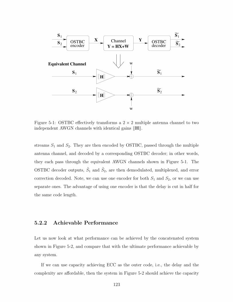
1S
S2
S1
S2
HS2 S2
S11SH
OSTBCencoder
Channel OSTBCdecoder
YX
w
Equivalent Channel w
Y = HX+W
Figure 5-1: OSTBC effectively transforms a 2 × 2 multiple antenna channel to twoindependent AWGN channels with identical gains ‖H‖.
streams S1 and S2. They are then encoded by OSTBC, passed through the multiple
antenna channel, and decoded by a corresponding OSTBC decoder; in other words,
they each pass through the equivalent AWGN channels shown in Figure 5-1. The
OSTBC decoder outputs, S1 and S2, are then demodulated, multiplexed, and error
correction decoded. Note, we can use one encoder for both S1 and S2, or we can use
separate ones. The advantage of using one encoder is that the delay is cut in half for
the same code length.
5.2.2 Achievable Performance
Let us now look at what performance can be achieved by the concatenated system
shown in Figure 5-2, and compare that with the ultimate performance achievable by
any system.
If we can use capacity achieving ECC as the outer code, i.e., the delay and the
complexity are affordable, then the system in Figure 5-2 should achieve the capacity
123
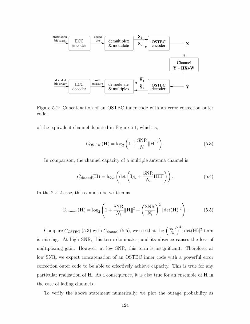
OSTBCencoder
OSTBCdecoder
Y = HX+WChannel
1S
S2
S2
S1
ECCencoder
demultiplex& modulate X
YECCdecoder
demodulate& multiplex
bit streaminformation
bit streamdecoded soft
measure
codedbits
Figure 5-2: Concatenation of an OSTBC inner code with an error correction outercode.
of the equivalent channel depicted in Figure 5-1, which is,
COSTBC(H) = log2
(1 +
SNR
Nt
‖H‖2). (5.3)
In comparison, the channel capacity of a multiple antenna channel is
Cchannel(H) = log2
(det
(INr
+SNR
Nt
HH†))
. (5.4)
In the 2× 2 case, this can also be written as
Cchannel(H) = log2
(1 +
SNR
Nt
‖H‖2 +(SNR
Nt
)2
| det(H)|2). (5.5)
Compare COSTBC (5.3) with Cchannel (5.5), we see that the(SNRNt
)2| det(H)|2 term
is missing. At high SNR, this term dominates, and its absence causes the loss of
multiplexing gain. However, at low SNR, this term is insignificant. Therefore, at
low SNR, we expect concatenation of an OSTBC inner code with a powerful error
correction outer code to be able to effectively achieve capacity. This is true for any
particular realization of H. As a consequence, it is also true for an ensemble of H in
the case of fading channels.
To verify the above statement numerically, we plot the outage probability as
124
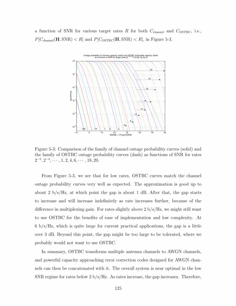
a function of SNR for various target rates R for both Cchannel and COSTBC, i.e.,
P [Cchannel(H, SNR) < R] and P [COSTBC(H, SNR) < R], in Figure 5-3.
−10 0 10 20 30 40 50 60
10−5
10−4
10−3
10−2
10−1
100
SNRdB = 10*log10(SNR)
log1
0(P
out)
Outage probability of channel capacity (solid) and OSTBC achievable capacity (dash) as functions of SNR for target rates [2.−5:1:0 2:2:20]. N
t=N
r=2
1/32 1/4 1 2 4
6
8
10
12
14
16
18
20
Figure 5-3: Comparison of the family of channel outage probability curves (solid) andthe family of OSTBC outage probability curves (dash) as functions of SNR for rates2−5, 2−4, · · · , 1, 2, 4, 6, · · · , 18, 20.
From Figure 5-3, we see that for low rates, OSTBC curves match the channel
outage probability curves very well as expected. The approximation is good up to
about 2 b/s/Hz, at which point the gap is about 1 dB. After that, the gap starts
to increase and will increase indefinitely as rate increases further, because of the
difference in multiplexing gain. For rates slightly above 2 b/s/Hz, we might still want
to use OSTBC for the benefits of ease of implementation and low complexity. At
6 b/s/Hz, which is quite large for current practical applications, the gap is a little
over 3 dB. Beyond this point, the gap might be too large to be tolerated, where we
probably would not want to use OSTBC.
In summary, OSTBC transforms multiple antenna channels to AWGN channels,
and powerful capacity approaching error correction codes designed for AWGN chan-
nels can then be concatenated with it. The overall system is near optimal in the low
SNR regime for rates below 2 b/s/Hz. As rates increase, the gap increases. Therefore,
125
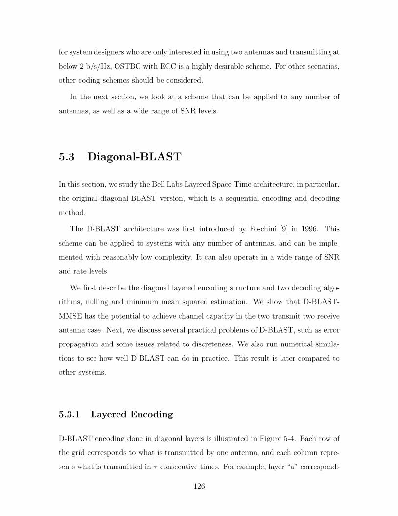
for system designers who are only interested in using two antennas and transmitting at
below 2 b/s/Hz, OSTBC with ECC is a highly desirable scheme. For other scenarios,
other coding schemes should be considered.
In the next section, we look at a scheme that can be applied to any number of
antennas, as well as a wide range of SNR levels.
5.3 Diagonal-BLAST
In this section, we study the Bell Labs Layered Space-Time architecture, in particular,
the original diagonal-BLAST version, which is a sequential encoding and decoding
method.
The D-BLAST architecture was first introduced by Foschini [9] in 1996. This
scheme can be applied to systems with any number of antennas, and can be imple-
mented with reasonably low complexity. It can also operate in a wide range of SNR
and rate levels.
We first describe the diagonal layered encoding structure and two decoding algo-
rithms, nulling and minimum mean squared estimation. We show that D-BLAST-
MMSE has the potential to achieve channel capacity in the two transmit two receive
antenna case. Next, we discuss several practical problems of D-BLAST, such as error
propagation and some issues related to discreteness. We also run numerical simula-
tions to see how well D-BLAST can do in practice. This result is later compared to
other systems.
5.3.1 Layered Encoding
D-BLAST encoding done in diagonal layers is illustrated in Figure 5-4. Each row of
the grid corresponds to what is transmitted by one antenna, and each column repre-
sents what is transmitted in τ consecutive times. For example, layer “a” corresponds
126

0 τ τ τ τ τ ττ ττ
3
1
2
4
5
6
(associatedtransmitter
Space
elements)
z
z
z
z
z
Time
y
a
y
y
y
2 3 5 6 7 8 94
a
a
a
a
a
b
b
b
b
b
b
c
c
c
c
c
x
d
d
d
d
e
e
e
f
f
f
hg
g
h i
w
d
ed f g
c e
x
v w x
Figure 5-4: BLAST encodes in diagonal layers labeled with different alphabeticalletters.
to the following entries in the transmitted signal matrix,
x1,1 · · · x1,τ
x2,τ+1 · · · x2,2τ. . .
xNt,Ntτ+1−τ · · · xNt,Ntτ
.
(5.6)
To perform encoding, we first encode raw information bits into codewords of length
Ntτ using any suitable coding scheme. Each codeword is then associated with one di-
agonal layer (with Ntτ entries) for transmission during the appropriate slots according
to Figure 5-4.
The key features of this encoding scheme are
1) all Ntτ symbols of a codeword are transmitted during different times, and
2) each codeword is transmitted (in pieces) by all antennas.
The reason for transmitting one codeword using all possible antennas is to maxi-
mize the tolerance of some of the channel coefficients being in deep-fade. The reason
for transmitting in different times is so that the symbols from the same codeword do
not interference with each other, which allows for convenient decoding as we illustrate
next.
127

5.3.2 Layered Decoding
In D-BLAST decoding, the diagonally-layered codewords are decoded one at a time, in
order, via successive cancellation. We first briefly describe how successive cancellation
is done to handle the interference between the layers, then describe how each layer
can be decoded.
Suppose we want to decode the layer labeled “a” in Figure 5-4. By this time, layers
“z” and before should have already been decoded. Therefore, we can completely
cancel out their interference on layer “a”. However, layers “b” and later have not
been decoded, so their interference remains. Two ways of handling these interference
are described in detail in the next two sections.
After handling the interference between the layers, each symbol of layer “a” is then
simply corrupted by some effective additive noise. There might be different amount
of noise on different symbols, and the coding applied would allow symbols that are
more reliable to help decode the ones that are not.
We decode each layer as if it had just gone through a varying gain AWGN channel.
One way is to do a two stage decoding. First all the symbols in that layer are indi-
vidually detected. The intermediate result can be in the form of either soft decision
or hard decision. The entire block is then passed on to the decoder where the original
information is extracted.
Next, let us describe in more detail the two ways of handling the interference
between layers, BLAST-nulling and BLAST-MMSE, and see what performance can
be achieved. These two methods are both based on successive cancellation and differ
in the way they handle the interference from the layers that have not been decoded.
BLAST-nulling
The BLAST-nulling scheme was earlier reviewed in section 3.2, and is briefly sum-
marized here. BLAST-nulling uses successive cancellation to cancel out interference
from layers already decoded and use Gram-Schmidt or QR factorization to null out
layers that have not been by only looking in the dimension orthogonal to all the
128

interference.
Let us suppose that we want to detect the entry x2,2τ of layer “a”. The received
signal vector at time 2τ is y2τ = Hx2τ + w2τ . The entries xi,2τ , i > 2, have been
decoded, and x1,2τ has not been.
We first factorize the channel matrix as H = QR, where Q is unitary and R is
upper triangular. y2τ can then be pre-processed to obtain y′2τ = Q†y2τ = Rx2τ+w
′2τ ,
where w′2τ = Q†w2τ and † denotes the conjugate transpose operation, so
y′1,2τ
y′2,τ...
y′Nt,2τ
=
r11 r12 · · · r1Nt
0 r22 · · · r2Nt
.... . . . . .
...
0 · · · 0 rNtNt
x1,2τ
x2,2τ...
xNt,2τ
+
w′1,2τ
w′2,2τ...
w′Nt,2τ
. (5.7)
Focus on the second row of the above matrix equation,
y′2,2τ = r22x2,2τ + r23x3,2τ + · · ·+ r2NtxNt,2τ + w′2,2τ , (5.8)
we see that the undecoded entry x1,2τ does not appear due to the nulling, and the
already decoded entries xi,2τ , i > 2, can be canceled out, leaving
y2,2τ = r22x2,2τ + w′2,2τ . (5.9)
Now, we can detect x2,2τ . Notice that if some of the entries xi,2τ , i > 2 were mis-
decoded, wrong values would have been canceled out, and x2,2τ might be mis-decoded
as well. This phenomenon is known as error propagation.
Once we detect all entires of layer “a” in similar fashion, we send the entire block
into a decoder to correct for any detection errors and get the transmitted codeword.
The BLAST-nulling decoding scheme is summarized in Figure 5-5.
To see what fraction of the total capacity can be achieved by such a system,
we note that the effective channel gain experienced by x2,2τ is r22. Similarly, the
channel gain experienced by entry xi,j is rii. So by using the BLAST architecture
129
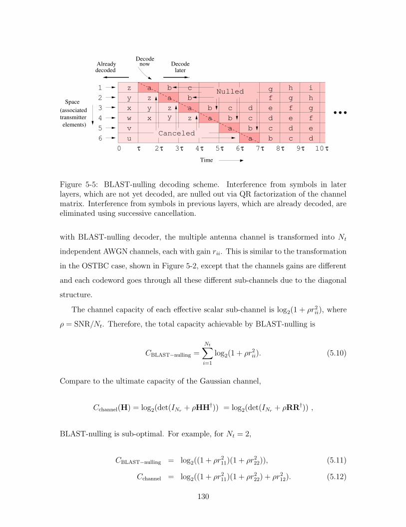
3
z
Canceled
Nulledz
z
z
laterAlready now
Decode
Time
1
2
4
5
6
(associatedtransmitter
Space
elements)
Decodedecoded
0 τ τ τ τ τ ττ ττ τ
y
y
u
a
y
a
a
a
a
a
b
b
b
b
b
b
v
w
c
c
c
c
c
x
x
d
d
d
d
e
e
e
f
f
f
hg
g
g
h i
2 3 5 6 7 8 9 104
Figure 5-5: BLAST-nulling decoding scheme. Interference from symbols in laterlayers, which are not yet decoded, are nulled out via QR factorization of the channelmatrix. Interference from symbols in previous layers, which are already decoded, areeliminated using successive cancellation.
with BLAST-nulling decoder, the multiple antenna channel is transformed into Nt
independent AWGN channels, each with gain rii. This is similar to the transformation
in the OSTBC case, shown in Figure 5-2, except that the channels gains are different
and each codeword goes through all these different sub-channels due to the diagonal
structure.
The channel capacity of each effective scalar sub-channel is log2(1 + ρr2ii), where
ρ = SNR/Nt. Therefore, the total capacity achievable by BLAST-nulling is
CBLAST−nulling =Nt∑
i=1
log2(1 + ρr2ii). (5.10)
Compare to the ultimate capacity of the Gaussian channel,
Cchannel(H) = log2(det(INr+ ρHH†)) = log2(det(INr
+ ρRR†)) ,
BLAST-nulling is sub-optimal. For example, for Nt = 2,
CBLAST−nulling = log2((1 + ρr211)(1 + ρr222)), (5.11)
Cchannel = log2((1 + ρr211)(1 + ρr222) + ρr212). (5.12)
130
BLAST-nulling utilizes only the diagonal elements of R and disregards the off
diagonal terms, causing it to be sub-optimal. In the limit of high SNR, the difference
can become arbitrarily small. However, it is still less robust against fading, since
having small diagonal terms for R would by sufficient to kill the transmission. We
do not get any protection from the off diagonal terms. Although BLAST-nulling is
sub-optimal, it is an efficient decoding scheme.
BLAST-MMSE
BLAST-MMSE is a variation of BLAST-nulling. In this section, we describe how they
differ and analyze the performance achievable by BLAST-MMSE in the two-transmit
two-receive antenna case. We show that while BLAST-nulling is sub-optimal, BLAST-
MMSE can actually achieve the full channel capacity by utilizing the off diagonal
terms of R.
The main difference between BLAST-MMSE and BLAST-nulling is how they
handle interference from entries that have not been decoded. In equation (5.7), where
y′2τ = Rx2τ +w′2τ is written out in full matrix form, instead of focusing only on the
second row to decode x2,2τ , we use the first two rows. We subtract out the already
decoded terms xi,2τ , i > 2, leaving
y2,2τ =
y1,2τ
y2,2τ
=
r11 r12
0 r22
x1,2τ
x2,2τ
+
w′1,2τ
w′2,2τ
. (5.13)
Since we want to detect x2,2τ only, we can treat x1,2τ as noise, combine the two noise
terms, and rewrite the above equation as
y2,2τ =
r12
r22
x2,2τ +
r11
0
x1,2τ +
w′1,2τ
w′2,2τ
=
r12
r22
x2,2τ +
v1,2τ
v2,2τ
. (5.14)
We can now find the MMSE of x2,2τ using the appropriate noise covariance matrix.
It turns out that the resulting effective SNR is ρr222 + ρr212/(1 + ρr211), instead of
ρr222 as is the case in BLAST-nulling. So by using the BLAST architecture with
131
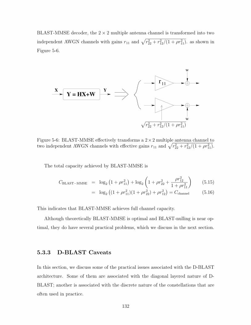
BLAST-MMSE decoder, the 2× 2 multiple antenna channel is transformed into two
independent AWGN channels with gains r11 and√r222 + r212/(1 + ρr211). as shown in
Figure 5-6.
w
w
Y = HX+WX Y
11r
√r222 + r212/(1 + ρr211)
Figure 5-6: BLAST-MMSE effectively transforms a 2×2 multiple antenna channel totwo independent AWGN channels with effective gains r11 and
√r222 + r212/(1 + ρr211).
The total capacity achieved by BLAST-MMSE is
CBLAST−MMSE = log2(1 + ρr211
)+ log2
(1 + ρr222 +
ρr2121 + ρr211
)(5.15)
= log2((1 + ρr211)(1 + ρr222) + ρr212
)= Cchannel (5.16)
This indicates that BLAST-MMSE achieves full channel capacity.
Although theoretically BLAST-MMSE is optimal and BLAST-nulling is near op-
timal, they do have several practical problems, which we discuss in the next section.
5.3.3 D-BLAST Caveats
In this section, we discuss some of the practical issues associated with the D-BLAST
architecture. Some of them are associated with the diagonal layered nature of D-
BLAST; another is associated with the discrete nature of the constellations that are
often used in practice.
132
Layered Structure Problems
Some of the problems with the diagonal layered structure are error propagation,
additional re-initialization cost, and increased delay.
Let us first discuss error propagation. Because decoding later layers requires the
previous layers to be correctly decoded, once one layer is mis-decoded, the error
will propagate on to later layers and may not stop for several layers. To reduce
error propagation, we must protect each layer with sufficiently strong error correction
codes. However, even if we do so, there might still be unpredictable events which
could cause occasional errors. If each of such events causes subsequent errors due to
propagation, it would make the system less robust.
One sure way to stop error propagation is to reinitialize, stop transmitting for
several layers and start transmitting a new layer without having to cancel previous
ones. However, this would increase the overhead associated with the initialization.
Because of the diagonal layered architecture, the lower triangle before the first layer
must all be initialized to zero or some known value to allow decoding of the first layer.
In the case of Nt = 2, this overhead is equal to half of a code block. For larger Nt,
the overhead would be even greater. To reduce the impact of overhead, we would
want to transmit many layers before re-initializing. However, this would lead us back
to the error propagation problem. Also, if the channel varies sufficiently fast and
come in and out of fade every few layers, then due to the error propagation, we must
reinitialize every time the channel comes out of a fade. This would lead to a lot of
re-initialization overhead.
The last problem associated with the layered structure that we would like to
mention is increased delay. For a given code length, spreading the codeword out in a
diagonal form so that only one symbol is transmitted at a time increases the delay by
a factor of Nt, compared to simply using all antennas to transmit at the same time.
Accompanying the increased delay, there is also increased buffering need, which for
long codewords (needed to reduce error propagation) might cause a practical problem.
133
Discrete Interference
One problem associated with BLAST-MMSE is that it treats all interference from
layers that have not been decoded as Gaussian noise, while in practice, they are often
chosen out of QAM-like constellations. This mis-match could lead to performance
degradation that are unnecessary.
More specifically, from (5.14), we see that when x2 (let us drop the timing index for
convenience) is being decoded, the effective noise is a combination of x1 and the actual
additive white Gaussian noise w′. If x1 has Gaussian distribution, the combined noise
would also be Gaussian. In this case, the MMSE estimator is also the ML estimator,
making MMSE a very good choice. However, in practice, Gaussian input distribution
is never used. Instead, regular constellation such as 16-QAM and 64-QAM are used.
In this case, the combined noise would not be Gaussian. In fact, if r11 is really large,
the noise distribution would look like a set of impulses, very different from Gaussian.
They simply have the same variance. It is well known that Gaussian distribution has
the largest entropy for a given variance. Therefore, the Gaussian noise approximation
would be overly pessimistic.
We might be able to take advantage of the fact that x1 is discrete by treating
the signal constellation as a lattice rather than incorrectly treating it as a continuous
Gaussian distribution. For example, when the channel is near singular, i.e., r11 is
much larger compared to r22, the received constellation points Hx might be close
to being “co-planer”, but they might still be well separated. We would be able to
tell which constellation point is transmitted. However, if we treat x1 as a continu-
ous Gaussian noise with a large variance, we would have a hard time detecting x2.
Later in section 5.6, we use a lattice-aware detector to treat the discreteness of the
constellation. The simulation result shows that there is in fact a small gain.
Finite Constellation Size Problem
Another practical problem associated with BLAST is what we call the finite con-
stellation size problem. The problem is that the amount of information that can be
134
carried is not only limited by the channel capacity, but also by the constellation size
used. Recall that BLAST effectively transforms a multiple antenna channel to mul-
tiple single antenna channels. The stronger sub-channels are expected to carry more
information than the weaker sub-channels. However, if the constellation used is too
small, then stronger sub-channels might not be able to carry as much information it
otherwise can. This could potentially prevent the total channel capacity from being
achieved.
In this section, we investigate how this phenomenon affects the system perfor-
mance. We show using both theoretical analysis and numerical simulation that using
a constellations that is too small can lead to a loss of diversity gain. We then discuss
how to choose the constellation size so that the performance loss is acceptable and
the constellation is not unnecessarily large. We propose to set the constellation size
to M2 = min(1 + SNR, 2R) or slightly larger.
In the two transmit two receive antenna case, the BLAST effectively transforms
the multiple antenna channel to two sub-channels. When MMSE detection is used,
combined capacity achievable is (5.15)
CBLAST−MMSE = log2(1 + ρr211
)+ log2
(1 + ρr222 +
ρr2121 + ρr211
).
Achieving this capacity assumes usage of Gaussian input distribution. However,
in practice, only finite constellations are used, in which case, the capacity achievable
by each sub-channel is upper bounded by log2(M2), where M 2 is the size of the QAM
constellation used. So the total capacity achievable is instead
CBLAST−MMSE,M=log2(min
(1 + ρr211,M
2))
+ log2
(min
(1 + ρr222 +
ρr2121 + ρr211
,M2
)).
Ideally, we would like to have CBLAST−MMSE,M > R whenever CBLAST−MMSE > R,
so that there is no loss in outage probability due to finite constellation size.
The problem associated with finite constellation arises when the constellation size
is small compared to the rate, i.e., M 2 < 2R. In this case, if one of the sub-channel
is in a sufficiently deep fade, i.e., the associated capacity is less then R − log2(M2),
135
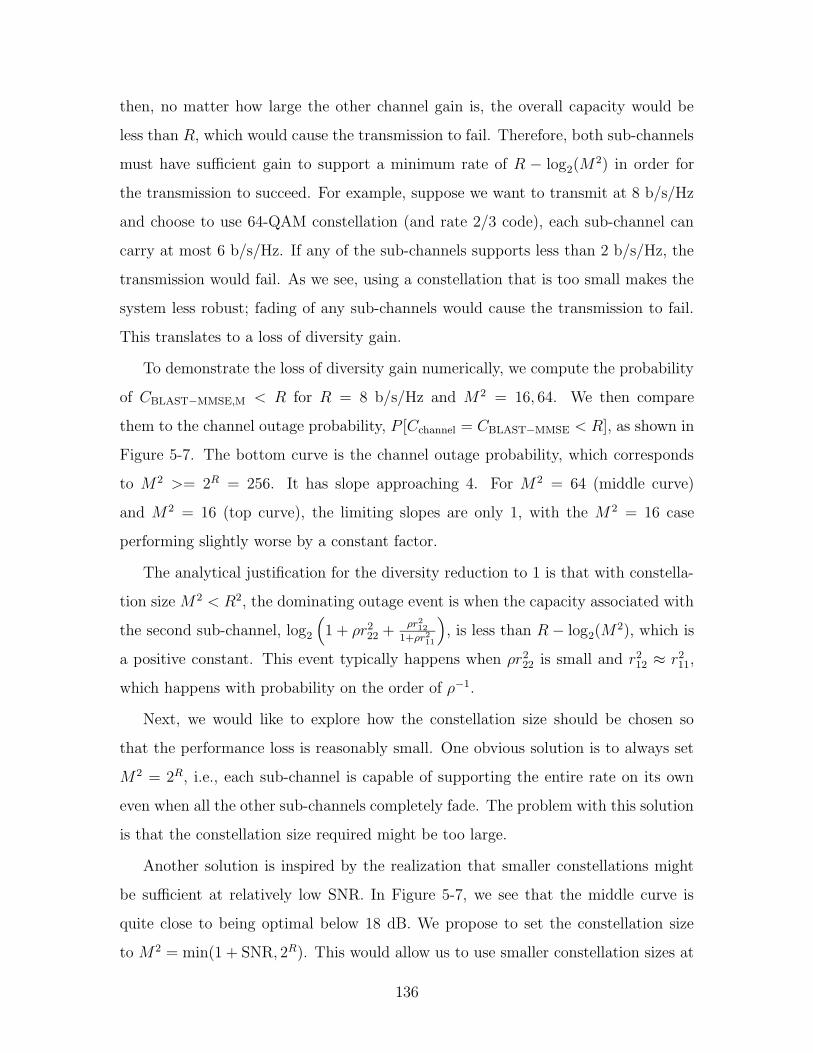
then, no matter how large the other channel gain is, the overall capacity would be
less than R, which would cause the transmission to fail. Therefore, both sub-channels
must have sufficient gain to support a minimum rate of R − log2(M2) in order for
the transmission to succeed. For example, suppose we want to transmit at 8 b/s/Hz
and choose to use 64-QAM constellation (and rate 2/3 code), each sub-channel can
carry at most 6 b/s/Hz. If any of the sub-channels supports less than 2 b/s/Hz, the
transmission would fail. As we see, using a constellation that is too small makes the
system less robust; fading of any sub-channels would cause the transmission to fail.
This translates to a loss of diversity gain.
To demonstrate the loss of diversity gain numerically, we compute the probability
of CBLAST−MMSE,M < R for R = 8 b/s/Hz and M 2 = 16, 64. We then compare
them to the channel outage probability, P [Cchannel = CBLAST−MMSE < R], as shown in
Figure 5-7. The bottom curve is the channel outage probability, which corresponds
to M2 >= 2R = 256. It has slope approaching 4. For M 2 = 64 (middle curve)
and M2 = 16 (top curve), the limiting slopes are only 1, with the M 2 = 16 case
performing slightly worse by a constant factor.
The analytical justification for the diversity reduction to 1 is that with constella-
tion size M 2 < R2, the dominating outage event is when the capacity associated with
the second sub-channel, log2
(1 + ρr222 +
ρr2121+ρr211
), is less than R− log2(M
2), which is
a positive constant. This event typically happens when ρr222 is small and r212 ≈ r211,
which happens with probability on the order of ρ−1.
Next, we would like to explore how the constellation size should be chosen so
that the performance loss is reasonably small. One obvious solution is to always set
M2 = 2R, i.e., each sub-channel is capable of supporting the entire rate on its own
even when all the other sub-channels completely fade. The problem with this solution
is that the constellation size required might be too large.
Another solution is inspired by the realization that smaller constellations might
be sufficient at relatively low SNR. In Figure 5-7, we see that the middle curve is
quite close to being optimal below 18 dB. We propose to set the constellation size
to M2 = min(1 + SNR, 2R). This would allow us to use smaller constellation sizes at
136
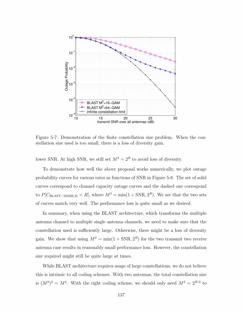
10 15 20 25 3010
−5
10−4
10−3
10−2
10−1
100
transmit SNR over all antennas (dB)
Out
age
Pro
babi
lity
BLAST M2=16−QAMBLAST M2=64−QAMinfinite constellation limit
Figure 5-7: Demonstration of the finite constellation size problem. When the con-stellation size used is too small, there is a loss of diversity gain.
lower SNR. At high SNR, we still set M 2 = 2R to avoid loss of diversity.
To demonstrate how well the above proposal works numerically, we plot outage
probability curves for various rates as functions of SNR in Figure 5-8. The set of solid
curves correspond to channel capacity outage curves and the dashed one correspond
to P [CBLAST−MMSE,M < R], where M 2 = min(1 + SNR, 2R). We see that the two sets
of curves match very well. The performance loss is quite small as we desired.
In summary, when using the BLAST architecture, which transforms the multiple
antenna channel to multiple single antenna channels, we need to make sure that the
constellation used is sufficiently large. Otherwise, there might be a loss of diversity
gain. We show that using M 2 = min(1 + SNR, 2R) for the two transmit two receive
antenna case results in reasonably small performance loss. However, the constellation
size required might still be quite large at times.
While BLAST architecture requires usage of large constellations, we do not believe
this is intrinsic to all coding schemes. With two antennas, the total constellation size
is (M 2)2 = M4. With the right coding scheme, we should only need M 2 = 2R/2 to
137
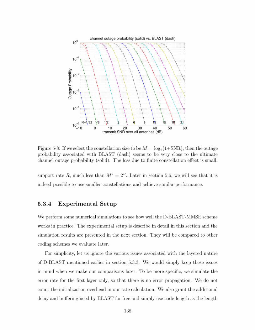
−10 0 10 20 30 40 50 6010
−5
10−4
10−3
10−2
10−1
100
transmit SNR over all antennas (dB)
Out
age
Pro
babi
lity
channel outage probability (solid) vs. BLAST (dash)
R=1/32 1/8 1/2 2 4 6 9 12 15 18 21
Figure 5-8: If we select the constellation size to beM = log2(1+SNR), then the outageprobability associated with BLAST (dash) seems to be very close to the ultimatechannel outage probability (solid). The loss due to finite constellation effect is small.
support rate R, much less than M 2 = 2R. Later in section 5.6, we will see that it is
indeed possible to use smaller constellations and achieve similar performance.
5.3.4 Experimental Setup
We perform some numerical simulations to see how well the D-BLAST-MMSE scheme
works in practice. The experimental setup is describe in detail in this section and the
simulation results are presented in the next section. They will be compared to other
coding schemes we evaluate later.
For simplicity, let us ignore the various issues associated with the layered nature
of D-BLAST mentioned earlier in section 5.3.3. We would simply keep these issues
in mind when we make our comparisons later. To be more specific, we simulate the
error rate for the first layer only, so that there is no error propagation. We do not
count the initialization overhead in our rate calculation. We also grant the additional
delay and buffering need by BLAST for free and simply use code-length as the length
138
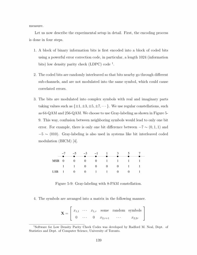
measure.
Let us now describe the experimental setup in detail. First, the encoding process
is done in four steps.
1. A block of binary information bits is first encoded into a block of coded bits
using a powerful error correction code, in particular, a length 1024 (information
bits) low density parity check (LDPC) code 1.
2. The coded bits are randomly interleaved so that bits nearby go through different
sub-channels, and are not modulated into the same symbol, which could cause
correlated errors.
3. The bits are modulated into complex symbols with real and imaginary parts
taking values such as ±1,±3,±5,±7, · · · . We use regular constellations, such
as 64-QAM and 256-QAM. We choose to use Gray-labeling as shown in Figure 5-
9. This way, confusion between neighboring symbols would lead to only one bit
error. For example, there is only one bit difference between −7 ∼ (0, 1, 1) and
−5 ∼ (010). Gray-labeling is also used in systems like bit interleaved coded
modulation (BICM) [4].
MSB 0 0 0 0 1 1 1 1
111 1
1
0 0 0 0
000 01 1 1LSB
−1 1 753−3−5−7
Figure 5-9: Gray-labeling with 8-PAM constellation.
4. The symbols are arranged into a matrix in the following manner.
X =
x1,1 · · · x1,τ some random symbols
0 · · · 0 x2,τ+1 · · · x2,2τ
1Software for Low Density Parity Check Codes was developed by Radford M. Neal, Dept. ofStatistics and Dept. of Computer Science, University of Toronto.
139
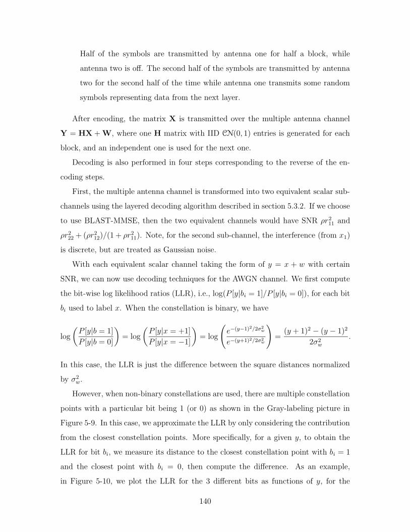
Half of the symbols are transmitted by antenna one for half a block, while
antenna two is off. The second half of the symbols are transmitted by antenna
two for the second half of the time while antenna one transmits some random
symbols representing data from the next layer.
After encoding, the matrix X is transmitted over the multiple antenna channel
Y = HX +W, where one H matrix with IID CN(0, 1) entries is generated for each
block, and an independent one is used for the next one.
Decoding is also performed in four steps corresponding to the reverse of the en-
coding steps.
First, the multiple antenna channel is transformed into two equivalent scalar sub-
channels using the layered decoding algorithm described in section 5.3.2. If we choose
to use BLAST-MMSE, then the two equivalent channels would have SNR ρr211 and
ρr222 + (ρr212)/(1 + ρr211). Note, for the second sub-channel, the interference (from x1)
is discrete, but are treated as Gaussian noise.
With each equivalent scalar channel taking the form of y = x + w with certain
SNR, we can now use decoding techniques for the AWGN channel. We first compute
the bit-wise log likelihood ratios (LLR), i.e., log(P [y|bi = 1]/P [y|bi = 0]), for each bit
bi used to label x. When the constellation is binary, we have
log
(P [y|b = 1]
P [y|b = 0]
)= log
(P [y|x = +1]
P [y|x = −1]
)= log
(e−(y−1)
2/2σ2w
e−(y+1)2/2σ2w
)=
(y + 1)2 − (y − 1)2
2σ2w.
In this case, the LLR is just the difference between the square distances normalized
by σ2w.
However, when non-binary constellations are used, there are multiple constellation
points with a particular bit being 1 (or 0) as shown in the Gray-labeling picture in
Figure 5-9. In this case, we approximate the LLR by only considering the contribution
from the closest constellation points. More specifically, for a given y, to obtain the
LLR for bit bi, we measure its distance to the closest constellation point with bi = 1
and the closest point with bi = 0, then compute the difference. As an example,
in Figure 5-10, we plot the LLR for the 3 different bits as functions of y, for the
140
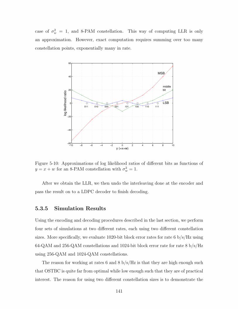
case of σ2w = 1, and 8-PAM constellation. This way of computing LLR is only
an approximation. However, exact computation requires summing over too many
constellation points, exponentially many in rate.
−10 −8 −6 −4 −2 0 2 4 6 8 10−60
−40
−20
0
20
40
60
011 010 000 001 101 100 110 111
MSB
LSB
middlebit
y (=x+w)
log
likel
ihoo
d ra
tio
Figure 5-10: Approximations of log likelihood ratios of different bits as functions ofy = x+ w for an 8-PAM constellation with σ2w = 1.
After we obtain the LLR, we then undo the interleaving done at the encoder and
pass the result on to a LDPC decoder to finish decoding.
5.3.5 Simulation Results
Using the encoding and decoding procedures described in the last section, we perform
four sets of simulations at two different rates, each using two different constellation
sizes. More specifically, we evaluate 1020-bit block error rates for rate 6 b/s/Hz using
64-QAM and 256-QAM constellations and 1024-bit block error rate for rate 8 b/s/Hz
using 256-QAM and 1024-QAM constellations.
The reason for working at rates 6 and 8 b/s/Hz is that they are high enough such
that OSTBC is quite far from optimal while low enough such that they are of practical
interest. The reason for using two different constellation sizes is to demonstrate the
141
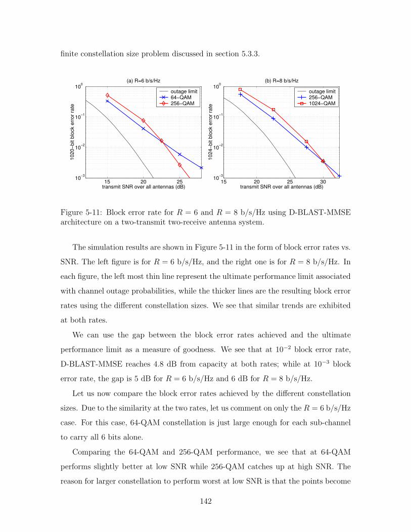
finite constellation size problem discussed in section 5.3.3.
15 20 2510−3
10−2
10−1
100
transmit SNR over all antennas (dB)
1020
−bit
bloc
k er
ror r
ate
(a) R=6 b/s/Hz
outage limit64−QAM256−QAM
15 20 25 3010−3
10−2
10−1
100
transmit SNR over all antennas (dB)
1024
−bit
bloc
k er
ror r
ate
(b) R=8 b/s/Hz
outage limit256−QAM1024−QAM
Figure 5-11: Block error rate for R = 6 and R = 8 b/s/Hz using D-BLAST-MMSEarchitecture on a two-transmit two-receive antenna system.
The simulation results are shown in Figure 5-11 in the form of block error rates vs.
SNR. The left figure is for R = 6 b/s/Hz, and the right one is for R = 8 b/s/Hz. In
each figure, the left most thin line represent the ultimate performance limit associated
with channel outage probabilities, while the thicker lines are the resulting block error
rates using the different constellation sizes. We see that similar trends are exhibited
at both rates.
We can use the gap between the block error rates achieved and the ultimate
performance limit as a measure of goodness. We see that at 10−2 block error rate,
D-BLAST-MMSE reaches 4.8 dB from capacity at both rates; while at 10−3 block
error rate, the gap is 5 dB for R = 6 b/s/Hz and 6 dB for R = 8 b/s/Hz.
Let us now compare the block error rates achieved by the different constellation
sizes. Due to the similarity at the two rates, let us comment on only the R = 6 b/s/Hz
case. For this case, 64-QAM constellation is just large enough for each sub-channel
to carry all 6 bits alone.
Comparing the 64-QAM and 256-QAM performance, we see that at 64-QAM
performs slightly better at low SNR while 256-QAM catches up at high SNR. The
reason for larger constellation to perform worst at low SNR is that the points become
142
too close compared to the noise level. When this happens, noise could carry the
original signal to many constellation points away. This makes decoding difficult. In
particular, our log likelihood ratio approximation, which only considers the closest
neighbors, becomes inaccurate.
The reason that 256-QAM catches up is related to the finite constellation size
problem. Although the 64-QAM constellation can carry 6 bits, it is insufficient be-
cause the LDPC code used is not capacity achieving. When one of the sub-channel
is in sufficiently deep fade, we can not recover the original codeword just from the 6
bits carried by the remaining sub-channel. From Figure 5-11 we see that the diversity
achieved by the 64-QAM constellation is smaller. This reflects the finite constellation
size effect. On the other hand, using 256-QAM would provide the additional margin
needed by the imperfect LDPC code. The slope achieved is similar to that of the
outage probability.
In summary, we studied the D-BLAST architecture in detail. In particular, we
show that D-BLAST-MMSE is theoretically optimal but have practical problems.
Our numerical simulations show that D-BLAST-MMSE can reach within 5 dB from
capacity.
5.4 Modified BLAST in Block Form
In the last section, we studied the original version of the BLAST architecture, D-
BLAST, which has a sequential form. In this section, we study three variations of
BLAST that are strictly block codes. The goal is to avoid the caveats associated with
the sequential nature of D-BLAST and explore different coding structures.
We first introduce these three different block-form variations, V-BLAST, two-
layer-D-BLAST, and X-BLAST, and describe their coding structures in section 5.4.1.
We then describe one common framework based on multiple access channel in which
all three schemes can be studied in section 5.4.2. The idea is to treat the multiple
codewords as messages from different users. In sections 5.4.3 to 5.4.5, we investigate
each scheme individually. We evaluate the achievable performance analytically, in
143

terms of both capacity and diversity-multiplexing tradeoff, when successive cancella-
tion based decoding is performed and when optimal joint decoding is done. We also
plot outage probability curves and compare them with the ultimate channel outage
performance limit. In section 5.4.6, we compare all three schemes along with OSTBC,
to see which method is the best in different SNR regimes, and where future potentials
lay.
All three schemes are described and analyzed in the two transmit antenna case.
The coding structure can be extended to higher dimensional cases, and the analysis
can potentially be done using the same framework, maybe with somewhat increased
complexity.
5.4.1 Code Designs
In this section, we introduce V-BLAST, two-layer-D-BLAST, and X-BLAST. The
first one is well known, while the latter two are new interesting structures that have
not been previously studied to our knowledge. The coding structures are described in
this section, while the analysis will be postponed until after we describe the common
framework in which all three schemes can be studied.
V-BLAST
The first variation of D-BLAST is the well-known V-BLAST, or vertical-BLAST
[39], which limits coding to each row of the transmitted signal matrix X as shown in
Figure 5-12 2. One codeword goes in the lighter region and the other one goes in the
darker region. V-BLAST was introduced after D-BLAST by the same group of people
as a simplified version of the original. However, there is a sacrifice in performance.
In V-BLAST, each codeword appears in only one row, i.e., coding takes place only
across time, but not across space. Because of this, V-BLAST is sub-optimal in the
sense that it achieves the maximum multiplexing gain, but not the maximum diversity
gain, as we will see later.
2The word vertical is used instead of horizontal because the transmitted signal matrix X waswritten in a transposed form in the original literature, relative to our formulation.
144
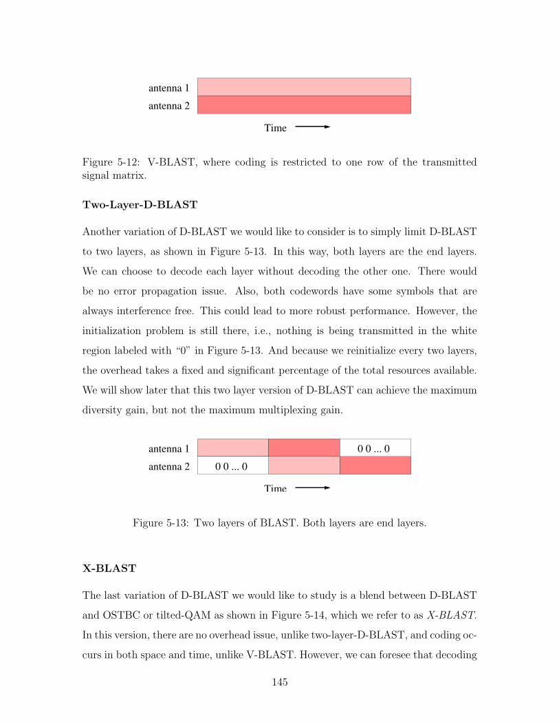
antenna 1
antenna 2
Time
Figure 5-12: V-BLAST, where coding is restricted to one row of the transmittedsignal matrix.
Two-Layer-D-BLAST
Another variation of D-BLAST we would like to consider is to simply limit D-BLAST
to two layers, as shown in Figure 5-13. In this way, both layers are the end layers.
We can choose to decode each layer without decoding the other one. There would
be no error propagation issue. Also, both codewords have some symbols that are
always interference free. This could lead to more robust performance. However, the
initialization problem is still there, i.e., nothing is being transmitted in the white
region labeled with “0” in Figure 5-13. And because we reinitialize every two layers,
the overhead takes a fixed and significant percentage of the total resources available.
We will show later that this two layer version of D-BLAST can achieve the maximum
diversity gain, but not the maximum multiplexing gain.
antenna 1
antenna 2
Time
0 0 ... 0
0 0 ... 0
Figure 5-13: Two layers of BLAST. Both layers are end layers.
X-BLAST
The last variation of D-BLAST we would like to study is a blend between D-BLAST
and OSTBC or tilted-QAM as shown in Figure 5-14, which we refer to as X-BLAST.
In this version, there are no overhead issue, unlike two-layer-D-BLAST, and coding oc-
curs in both space and time, unlike V-BLAST. However, we can foresee that decoding
145
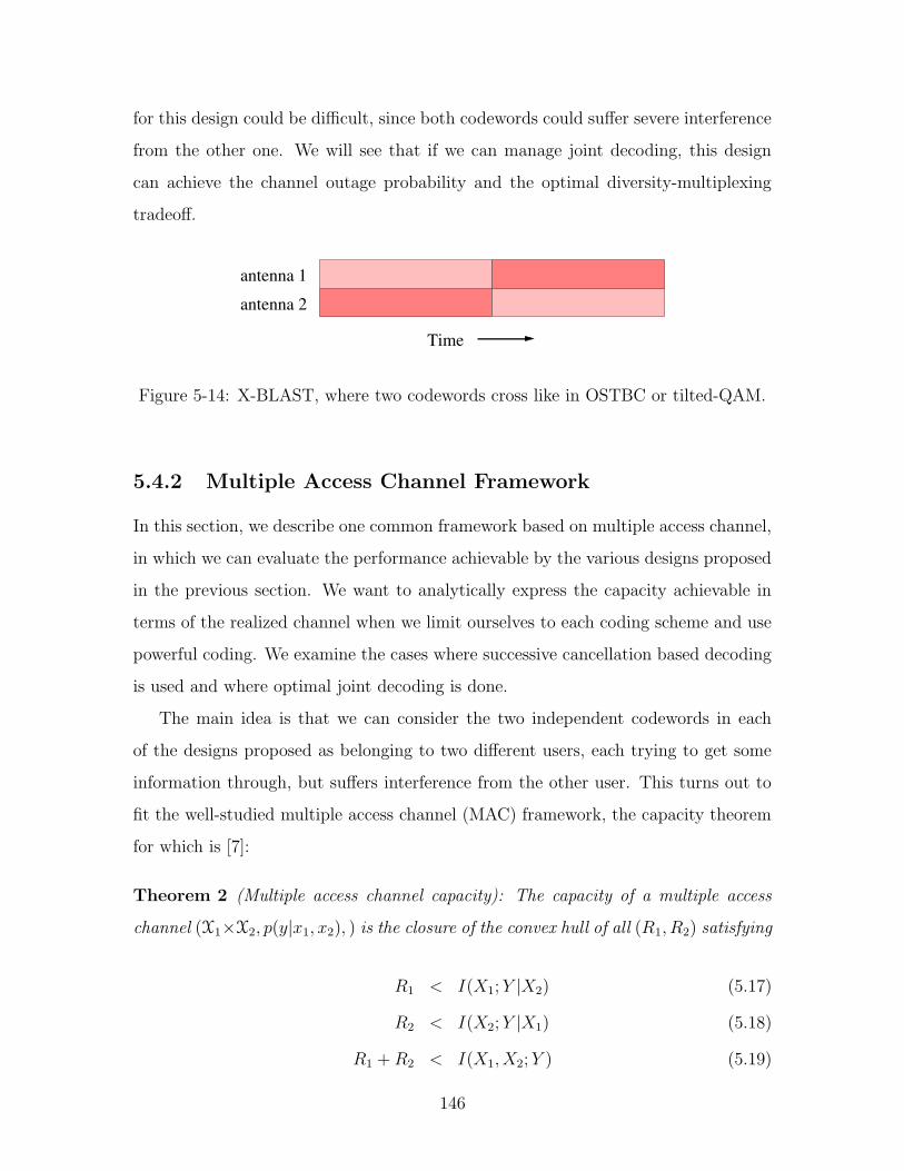
for this design could be difficult, since both codewords could suffer severe interference
from the other one. We will see that if we can manage joint decoding, this design
can achieve the channel outage probability and the optimal diversity-multiplexing
tradeoff.
antenna 1
antenna 2
Time
Figure 5-14: X-BLAST, where two codewords cross like in OSTBC or tilted-QAM.
5.4.2 Multiple Access Channel Framework
In this section, we describe one common framework based on multiple access channel,
in which we can evaluate the performance achievable by the various designs proposed
in the previous section. We want to analytically express the capacity achievable in
terms of the realized channel when we limit ourselves to each coding scheme and use
powerful coding. We examine the cases where successive cancellation based decoding
is used and where optimal joint decoding is done.
The main idea is that we can consider the two independent codewords in each
of the designs proposed as belonging to two different users, each trying to get some
information through, but suffers interference from the other user. This turns out to
fit the well-studied multiple access channel (MAC) framework, the capacity theorem
for which is [7]:
Theorem 2 (Multiple access channel capacity): The capacity of a multiple access
channel (X1×X2, p(y|x1, x2), ) is the closure of the convex hull of all (R1, R2) satisfying
R1 < I(X1;Y |X2) (5.17)
R2 < I(X2;Y |X1) (5.18)
R1 +R2 < I(X1, X2;Y ) (5.19)
146
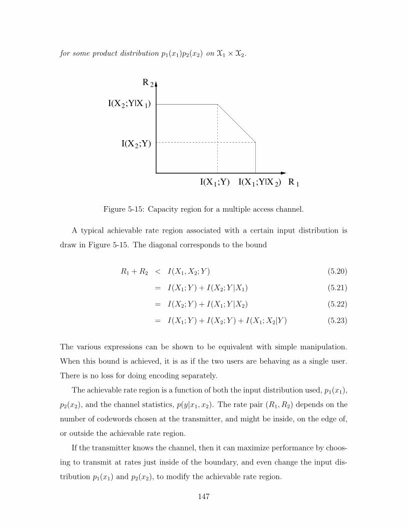
for some product distribution p1(x1)p2(x2) on X1 × X2.
R
R 1
2
2
I(X ;Y|X )12
I(X ;Y|X )1
I(X ;Y)
I(X ;Y)1
2
Figure 5-15: Capacity region for a multiple access channel.
A typical achievable rate region associated with a certain input distribution is
draw in Figure 5-15. The diagonal corresponds to the bound
R1 +R2 < I(X1, X2;Y ) (5.20)
= I(X1;Y ) + I(X2;Y |X1) (5.21)
= I(X2;Y ) + I(X1;Y |X2) (5.22)
= I(X1;Y ) + I(X2;Y ) + I(X1;X2|Y ) (5.23)
The various expressions can be shown to be equivalent with simple manipulation.
When this bound is achieved, it is as if the two users are behaving as a single user.
There is no loss for doing encoding separately.
The achievable rate region is a function of both the input distribution used, p1(x1),
p2(x2), and the channel statistics, p(y|x1, x2). The rate pair (R1, R2) depends on the
number of codewords chosen at the transmitter, and might be inside, on the edge of,
or outside the achievable rate region.
If the transmitter knows the channel, then it can maximize performance by choos-
ing to transmit at rates just inside of the boundary, and even change the input dis-
tribution p1(x1) and p2(x2), to modify the achievable rate region.
147
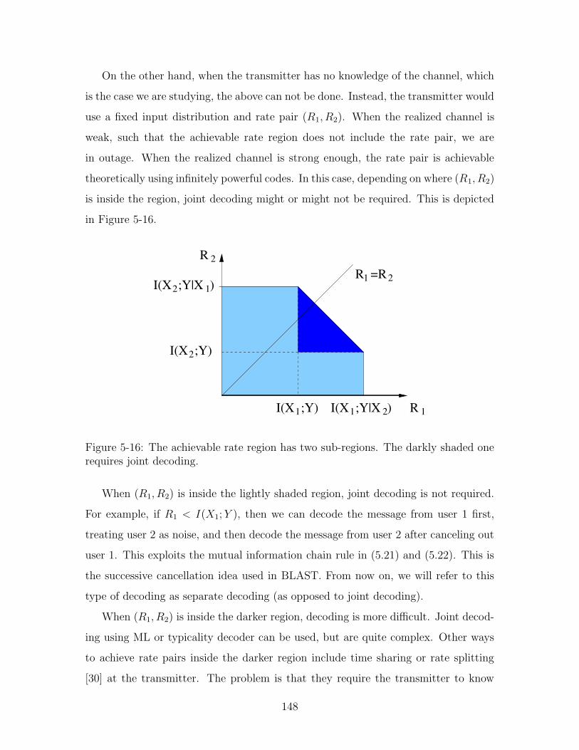
On the other hand, when the transmitter has no knowledge of the channel, which
is the case we are studying, the above can not be done. Instead, the transmitter would
use a fixed input distribution and rate pair (R1, R2). When the realized channel is
weak, such that the achievable rate region does not include the rate pair, we are
in outage. When the realized channel is strong enough, the rate pair is achievable
theoretically using infinitely powerful codes. In this case, depending on where (R1, R2)
is inside the region, joint decoding might or might not be required. This is depicted
in Figure 5-16.
I(X ;Y)2
I(X ;Y|X )12
I(X ;Y)1 2I(X ;Y|X )1 R 1
R =R1 2
R 2
Figure 5-16: The achievable rate region has two sub-regions. The darkly shaded onerequires joint decoding.
When (R1, R2) is inside the lightly shaded region, joint decoding is not required.
For example, if R1 < I(X1;Y ), then we can decode the message from user 1 first,
treating user 2 as noise, and then decode the message from user 2 after canceling out
user 1. This exploits the mutual information chain rule in (5.21) and (5.22). This is
the successive cancellation idea used in BLAST. From now on, we will refer to this
type of decoding as separate decoding (as opposed to joint decoding).
When (R1, R2) is inside the darker region, decoding is more difficult. Joint decod-
ing using ML or typicality decoder can be used, but are quite complex. Other ways
to achieve rate pairs inside the darker region include time sharing or rate splitting
[30] at the transmitter. The problem is that they require the transmitter to know
148
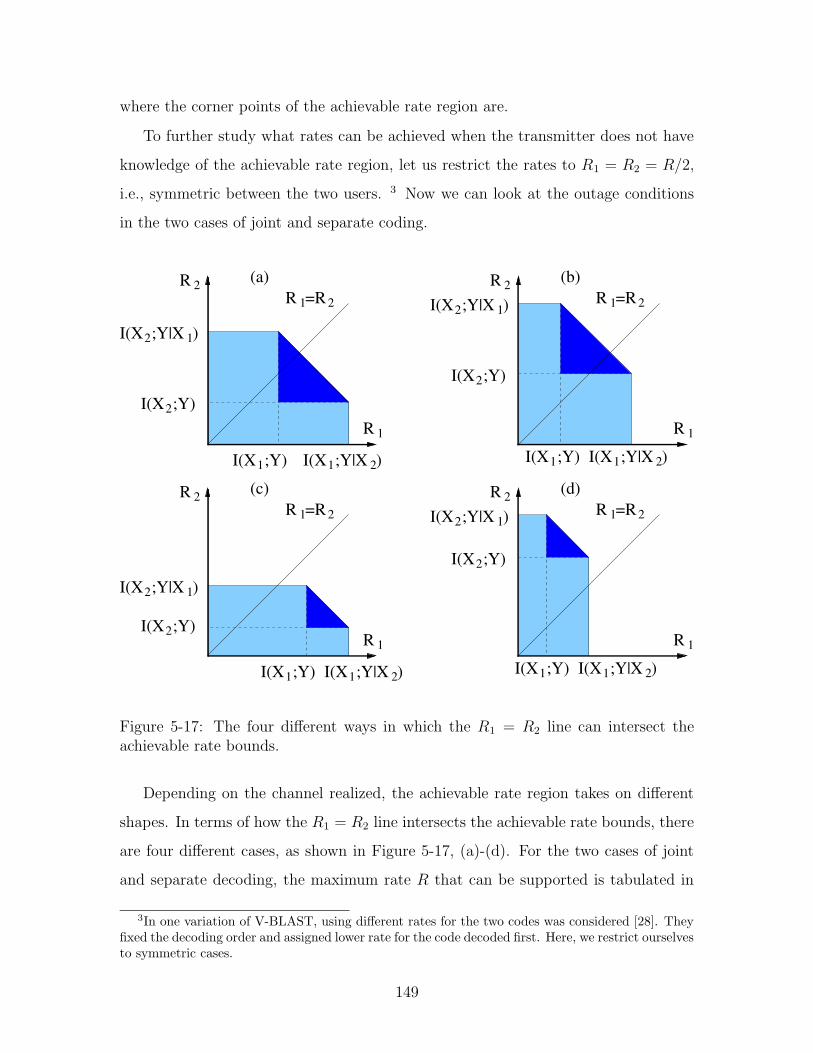
where the corner points of the achievable rate region are.
To further study what rates can be achieved when the transmitter does not have
knowledge of the achievable rate region, let us restrict the rates to R1 = R2 = R/2,
i.e., symmetric between the two users. 3 Now we can look at the outage conditions
in the two cases of joint and separate coding.
(a) (b)
(c) (d)
I(X ;Y)2
I(X ;Y)1 2I(X ;Y|X )1
I(X ;Y|X )12
I(X ;Y|X )12
I(X ;Y)2
2I(X ;Y|X )1I(X ;Y)1
R 1
R 2
I(X ;Y)2
I(X ;Y|X )12
I(X ;Y|X )12
I(X ;Y)2
R 2 R 2
R 1
2I(X ;Y|X )1I(X ;Y)1 2I(X ;Y|X )1I(X ;Y)1
R 1
R =R1 2
R =R1 2 R =R1 2
R =R1 2
R 2
R 1
Figure 5-17: The four different ways in which the R1 = R2 line can intersect theachievable rate bounds.
Depending on the channel realized, the achievable rate region takes on different
shapes. In terms of how the R1 = R2 line intersects the achievable rate bounds, there
are four different cases, as shown in Figure 5-17, (a)-(d). For the two cases of joint
and separate decoding, the maximum rate R that can be supported is tabulated in
3In one variation of V-BLAST, using different rates for the two codes was considered [28]. Theyfixed the decoding order and assigned lower rate for the code decoded first. Here, we restrict ourselvesto symmetric cases.
149
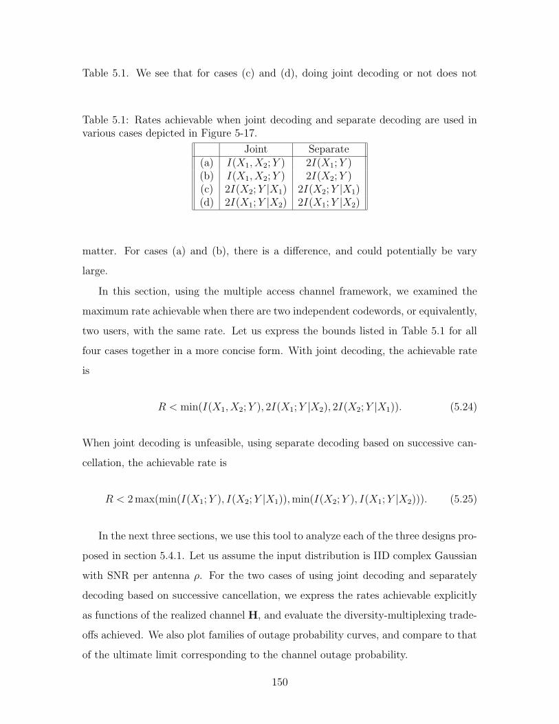
Table 5.1. We see that for cases (c) and (d), doing joint decoding or not does not
Table 5.1: Rates achievable when joint decoding and separate decoding are used invarious cases depicted in Figure 5-17.
Joint Separate(a) I(X1, X2;Y ) 2I(X1;Y )(b) I(X1, X2;Y ) 2I(X2;Y )(c) 2I(X2;Y |X1) 2I(X2;Y |X1)(d) 2I(X1;Y |X2) 2I(X1;Y |X2)
matter. For cases (a) and (b), there is a difference, and could potentially be vary
large.
In this section, using the multiple access channel framework, we examined the
maximum rate achievable when there are two independent codewords, or equivalently,
two users, with the same rate. Let us express the bounds listed in Table 5.1 for all
four cases together in a more concise form. With joint decoding, the achievable rate
is
R < min(I(X1, X2;Y ), 2I(X1;Y |X2), 2I(X2;Y |X1)). (5.24)
When joint decoding is unfeasible, using separate decoding based on successive can-
cellation, the achievable rate is
R < 2max(min(I(X1;Y ), I(X2;Y |X1)),min(I(X2;Y ), I(X1;Y |X2))). (5.25)
In the next three sections, we use this tool to analyze each of the three designs pro-
posed in section 5.4.1. Let us assume the input distribution is IID complex Gaussian
with SNR per antenna ρ. For the two cases of using joint decoding and separately
decoding based on successive cancellation, we express the rates achievable explicitly
as functions of the realized channel H, and evaluate the diversity-multiplexing trade-
offs achieved. We also plot families of outage probability curves, and compare to that
of the ultimate limit corresponding to the channel outage probability.
150
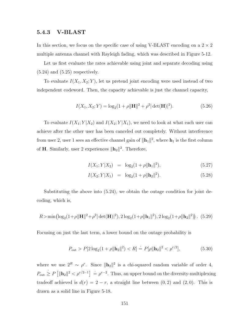
5.4.3 V-BLAST
In this section, we focus on the specific case of using V-BLAST encoding on a 2× 2
multiple antenna channel with Rayleigh fading, which was described in Figure 5-12.
Let us first evaluate the rates achievable using joint and separate decoding using
(5.24) and (5.25) respectively.
To evaluate I(X1, X2;Y ), let us pretend joint encoding were used instead of two
independent codeword. Then, the capacity achievable is just the channel capacity,
I(X1, X2;Y ) = log2(1 + ρ‖H‖2 + ρ2| det(H)|2). (5.26)
To evaluate I(X1;Y |X2) and I(X2;Y |X1), we need to look at what each user can
achieve after the other user has been canceled out completely. Without interference
from user 2, user 1 sees an effective channel gain of ‖h1‖2, where h1 is the first column
of H. Similarly, user 2 experiences ‖h2‖2. Therefore,
I(X1;Y |X2) = log2(1 + ρ‖h1‖2), (5.27)
I(X2;Y |X1) = log2(1 + ρ‖h2‖2). (5.28)
Substituting the above into (5.24), we obtain the outage condition for joint de-
coding, which is,
R>min(log2(1+ρ‖H‖2+ρ2| det(H)|2), 2 log2(1+ρ‖h1‖2), 2 log2(1+ρ‖h2‖2)
). (5.29)
Focusing on just the last term, a lower bound on the outage probability is
Pout > P [2 log2(1 + ρ‖h2‖2) < R]·= P [ρ‖h2‖2 < ρr/2], (5.30)
where we use 2R ∼ ρr. Since ‖h2‖2 is a chi-squared random variable of order 4,
Pout·≥ P
[‖h2‖2 < ρr/2−1
] ·= ρr−2. Thus, an upper bound on the diversity-multiplexing
tradeoff achieved is d(r) = 2 − r, a straight line between (0, 2) and (2, 0). This is
drawn as a solid line in Figure 5-18.
151
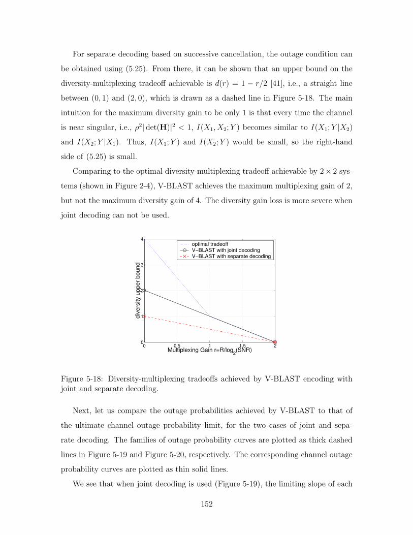
For separate decoding based on successive cancellation, the outage condition can
be obtained using (5.25). From there, it can be shown that an upper bound on the
diversity-multiplexing tradeoff achievable is d(r) = 1 − r/2 [41], i.e., a straight line
between (0, 1) and (2, 0), which is drawn as a dashed line in Figure 5-18. The main
intuition for the maximum diversity gain to be only 1 is that every time the channel
is near singular, i.e., ρ2| det(H)|2 < 1, I(X1, X2;Y ) becomes similar to I(X1;Y |X2)
and I(X2;Y |X1). Thus, I(X1;Y ) and I(X2;Y ) would be small, so the right-hand
side of (5.25) is small.
Comparing to the optimal diversity-multiplexing tradeoff achievable by 2× 2 sys-
tems (shown in Figure 2-4), V-BLAST achieves the maximum multiplexing gain of 2,
but not the maximum diversity gain of 4. The diversity gain loss is more severe when
joint decoding can not be used.
0 0.5 1 1.5 20
1
2
3
4
Multiplexing Gain r=R/log2(SNR)
dive
rsity
upp
er b
ound
optimal tradeoffV−BLAST with joint decodingV−BLAST with separate decoding
Figure 5-18: Diversity-multiplexing tradeoffs achieved by V-BLAST encoding withjoint and separate decoding.
Next, let us compare the outage probabilities achieved by V-BLAST to that of
the ultimate channel outage probability limit, for the two cases of joint and sepa-
rate decoding. The families of outage probability curves are plotted as thick dashed
lines in Figure 5-19 and Figure 5-20, respectively. The corresponding channel outage
probability curves are plotted as thin solid lines.
We see that when joint decoding is used (Figure 5-19), the limiting slope of each
152
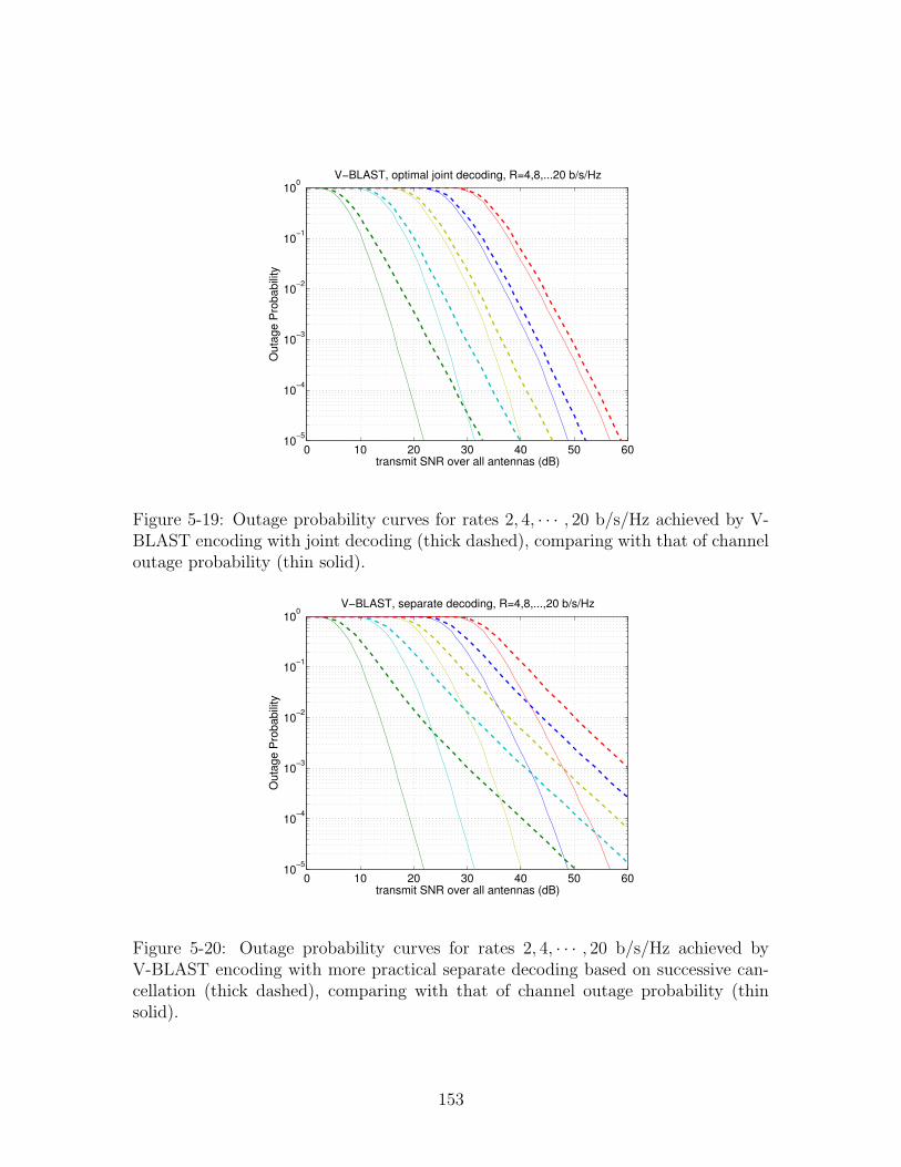
0 10 20 30 40 50 6010
−5
10−4
10−3
10−2
10−1
100
transmit SNR over all antennas (dB)
Out
age
Pro
babi
lity
V−BLAST, optimal joint decoding, R=4,8,...20 b/s/Hz
Figure 5-19: Outage probability curves for rates 2, 4, · · · , 20 b/s/Hz achieved by V-BLAST encoding with joint decoding (thick dashed), comparing with that of channeloutage probability (thin solid).
0 10 20 30 40 50 6010
−5
10−4
10−3
10−2
10−1
100
transmit SNR over all antennas (dB)
Out
age
Pro
babi
lity
V−BLAST, separate decoding, R=4,8,...,20 b/s/Hz
Figure 5-20: Outage probability curves for rates 2, 4, · · · , 20 b/s/Hz achieved byV-BLAST encoding with more practical separate decoding based on successive can-cellation (thick dashed), comparing with that of channel outage probability (thinsolid).
153

curve is only 2, which is sub-optimal compared to the channel outage probability
curves. However, for higher rates, this deficiency does not have a significant conse-
quence. V-BLAST with joint decoding is only 1 to 2 dB from optimal at 10−3 target
outage probability.
When separate decoding is used (Figure 5-20), the limiting slopes of each curve is
only 1, and there is a significant discrepancy between the outage probability curves
achieved and the performance limit. At 10−3 target outage probability, the gaps
between the corresponding solid and dashed curves are over 10 dB, and become even
larger for lower target outage probabilities.
We note that V-BLAST achieves the maximummultiplexing gain when either joint
decoding or separate decoding is use. Therefore, the spacings between the curves for
both cases are 2 bits per 3 dB, which is optimal. Therefore, for a fixed target error
rate, the gaps to the optimal curves approach constant values as rate increases.
5.4.4 Two-Layer-D-BLAST
Now let us turn to the two-layer-D-BLAST design illustrated in Figure 5-13. Com-
pared to the V-BLAST design we just studied, there are two main differences.
The first one is that this code effectively has three different segments as we can
see visually in Figure 5-13. Because of this, the mutual information achieved is the
average of the three region. We have,
I(X1,X2;Y )=1
3
(log2(1+ρ‖h1‖2)+log2(1+ρ‖H‖2+ρ2| det(H)|2)+log2(1+ρ‖h2‖2)
),
(5.31)
where the three terms corresponds to the left, middle, and right regions.
The other feature of this design, which is absent in V-BLAST, is the symmetry
between the two users in terms of the individual mutual information achieved. Also
using averaging, we have
I(X1;Y |X2) = I(X2;Y |X1) =1
3
(log2(1 + ρ‖h1‖2) + log2(1 + ρ‖h2‖2)
). (5.32)
154
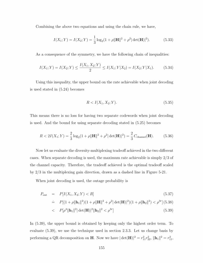
Combining the above two equations and using the chain rule, we have,
I(X1;Y ) = I(X2;Y ) =1
3log2(1 + ρ‖H‖2 + ρ2| det(H)|2). (5.33)
As a consequence of the symmetry, we have the following chain of inequalities:
I(X1;Y ) = I(X2;Y ) ≤ I(X1, X2;Y )
2≤ I(X1;Y |X2) = I(X2;Y |X1). (5.34)
Using this inequality, the upper bound on the rate achievable when joint decoding
is used stated in (5.24) becomes
R < I(X1, X2;Y ). (5.35)
This means there is no loss for having two separate codewords when joint decoding
is used. And the bound for using separate decoding stated in (5.25) becomes
R < 2I(X1;Y ) =2
3log2(1 + ρ‖H‖2 + ρ2| det(H)|2) = 2
3Cchannel(H). (5.36)
Now let us evaluate the diversity-multiplexing tradeoff achieved in the two different
cases. When separate decoding is used, the maximum rate achievable is simply 2/3 of
the channel capacity. Therefore, the tradeoff achieved is the optimal tradeoff scaled
by 2/3 in the multiplexing gain direction, drawn as a dashed line in Figure 5-21.
When joint decoding is used, the outage probability is
Pout = P [I(X1, X2;Y ) < R] (5.37)
·= P [(1 + ρ‖h1‖2)(1 + ρ‖H‖2 + ρ2| det(H)|2)(1 + ρ‖h2‖2) < ρ3r] (5.38)
< P [ρ4‖h1‖2| det(H)|2‖h2‖2 < ρ3r] (5.39)
In (5.39), the upper bound is obtained by keeping only the highest order term. To
evaluate (5.39), we use the technique used in section 2.3.3. Let us change basis by
performing a QR decomposition on H. Now we have | det(H)|2 = r211r222, ‖h1‖2 = r211,
155
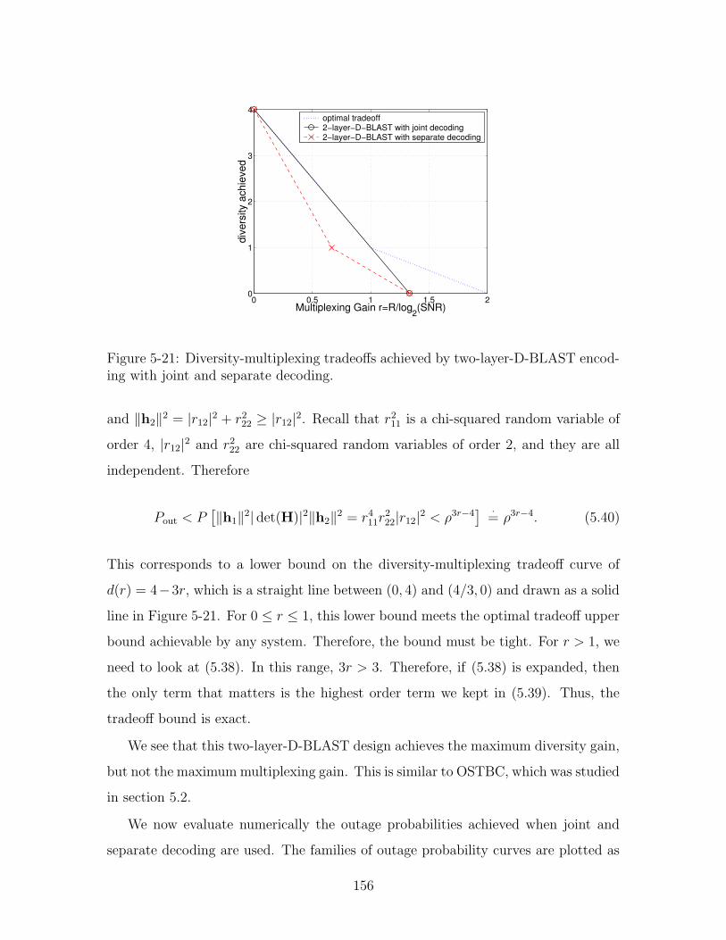
0 0.5 1 1.5 20
1
2
3
4
Multiplexing Gain r=R/log2(SNR)
dive
rsity
ach
ieve
d
optimal tradeoff2−layer−D−BLAST with joint decoding2−layer−D−BLAST with separate decoding
Figure 5-21: Diversity-multiplexing tradeoffs achieved by two-layer-D-BLAST encod-ing with joint and separate decoding.
and ‖h2‖2 = |r12|2 + r222 ≥ |r12|2. Recall that r211 is a chi-squared random variable of
order 4, |r12|2 and r222 are chi-squared random variables of order 2, and they are all
independent. Therefore
Pout < P[‖h1‖2| det(H)|2‖h2‖2 = r411r
222|r12|2 < ρ3r−4
] ·= ρ3r−4. (5.40)
This corresponds to a lower bound on the diversity-multiplexing tradeoff curve of
d(r) = 4−3r, which is a straight line between (0, 4) and (4/3, 0) and drawn as a solid
line in Figure 5-21. For 0 ≤ r ≤ 1, this lower bound meets the optimal tradeoff upper
bound achievable by any system. Therefore, the bound must be tight. For r > 1, we
need to look at (5.38). In this range, 3r > 3. Therefore, if (5.38) is expanded, then
the only term that matters is the highest order term we kept in (5.39). Thus, the
tradeoff bound is exact.
We see that this two-layer-D-BLAST design achieves the maximum diversity gain,
but not the maximummultiplexing gain. This is similar to OSTBC, which was studied
in section 5.2.
We now evaluate numerically the outage probabilities achieved when joint and
separate decoding are used. The families of outage probability curves are plotted as
156
thick dashed lines in Figure 5-22 and Figure 5-23, respectively. The corresponding
channel outage probability curves are plotted as thin solid lines for comparison.
Comparing to the optimal curves, we see that the outage probabilities achieved by
the two-layer-D-BLAST design have the same limiting slope, i.e., the same maximum
diversity. However, due to the sub-optimal multiplexing gain, the gap to optimality,
i.e., the gap between the corresponding solid and dashed curves grows indefinitely.
Therefore, this design should not be used at high SNR. Recall that this phenomenon
was also exhibited by OSTBC in Figure 5-3.
It is also worth noting that there is not a significant difference between using joint
decoding and using separate decoding. In the sense that they both have large gaps
at high SNR and non-zero gaps at low SNR.
5.4.5 X-BLAST
The last design to be analyzed is the X-BLAST design shown in Figure 5-14. This
design has complete symmetry between the two users. Using similar techniques as in
the previous cases, it can be shown that
I(X1, X2;Y ) = log2(1 + ρ‖H‖2 + ρ2| det(H)|2), (5.41)
I(X1;Y |X2) = I(X2;Y |X1) =1
2
(log2(1 + ρ‖h1‖2) + log2(1 + ρ‖h2‖2)
). (5.42)
Also due to symmetry, we have the same chain of inequalities as in (5.34). When
joint decoding is used, the maximum rate achievable is also I(X1, X2;Y ), which is
the same as the channel capacity for this design. Therefore, there is no loss for using
X-BLAST encoding when joint decoding is used.
When separate decoding is used, we have a situation similar to the V-BLAST case.
The quantity I(X1;Y |X2) + I(X2;Y |X1) equals log2(1 + ρ‖h1‖2) + log2(1 + ρ‖h2‖2)in both cases. The quantity I(X1;Y ) + I(X2;Y ) from both cases are also equal.
Together with the achievable rate upper bound in (5.25), these lead us to believe that
the diversity-multiplexing tradeoff achieved by X-BLAST with separate decoding is
the same as that by V-BLAST, which is d(r) = 1− r/2, a straight line between (0, 1)
157
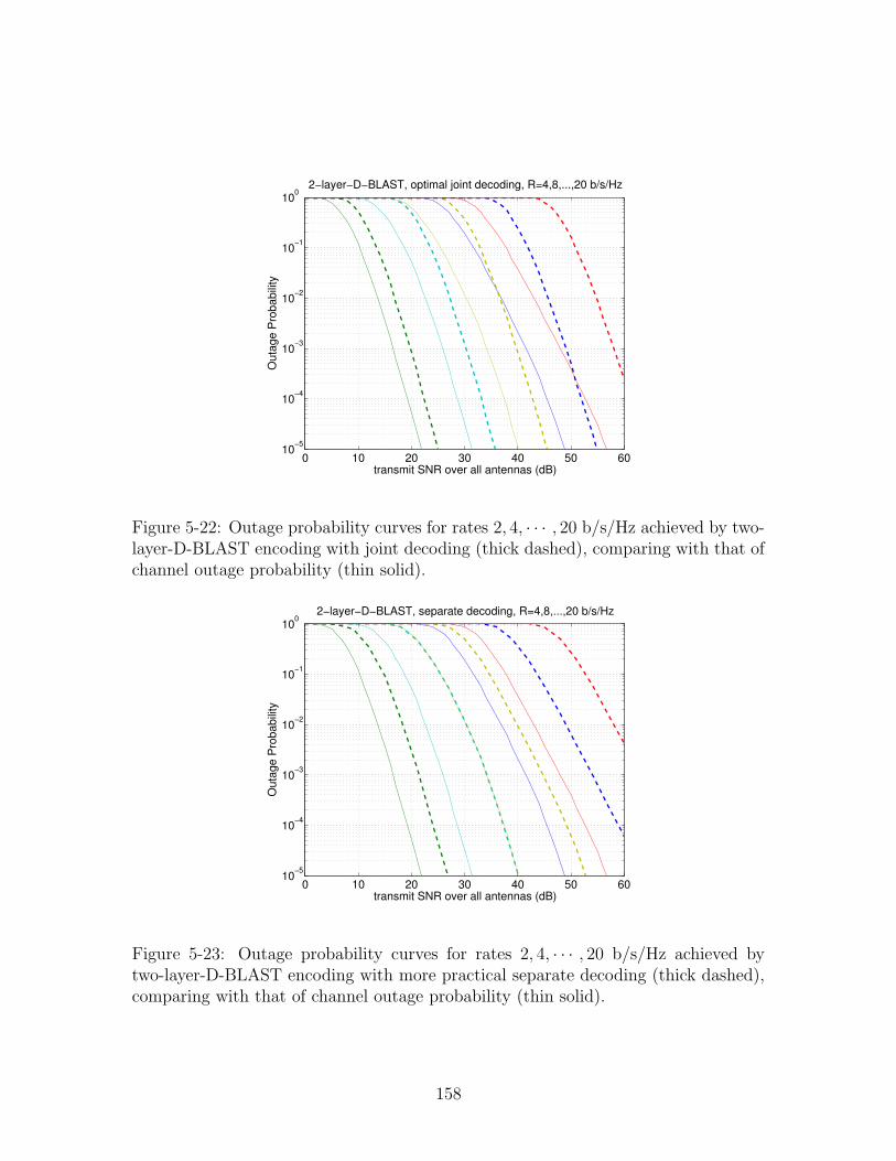
0 10 20 30 40 50 6010
−5
10−4
10−3
10−2
10−1
100
2−layer−D−BLAST, optimal joint decoding, R=4,8,...,20 b/s/Hz
transmit SNR over all antennas (dB)
Out
age
Pro
babi
lity
Figure 5-22: Outage probability curves for rates 2, 4, · · · , 20 b/s/Hz achieved by two-layer-D-BLAST encoding with joint decoding (thick dashed), comparing with that ofchannel outage probability (thin solid).
0 10 20 30 40 50 6010
−5
10−4
10−3
10−2
10−1
100
transmit SNR over all antennas (dB)
Out
age
Pro
babi
lity
2−layer−D−BLAST, separate decoding, R=4,8,...,20 b/s/Hz
Figure 5-23: Outage probability curves for rates 2, 4, · · · , 20 b/s/Hz achieved bytwo-layer-D-BLAST encoding with more practical separate decoding (thick dashed),comparing with that of channel outage probability (thin solid).
158

and (2, 0).
The tradeoff curves for both cases are drawn in Figure 5-24. We see that using
joint decoding yields the optimal tradeoff, while using separate decoding results in
significant loss in diversity gain, similar to V-BLAST.
0 0.5 1 1.5 20
1
2
3
4
Multiplexing Gain r=R/log2(SNR)
dive
rsity
ach
ieve
dCross−BLAST with joint decodingCross−BLAST with separate decoding
Figure 5-24: Diversity-multiplexing tradeoffs achieved by X-BLAST encoding withjoint and separate decoding.
We also evaluate numerically the outage probabilities achieved by X-BLAST when
joint decoding and separate decoding is used. The families of outage probability
curves are plotted as thick dashed lines in Figure 5-25.
When joint decoding is used, the optimal outage probability is achieved. When
separate decoding is used, the resulting outage probability curves are similar to that
of V-BLAST with separate decoding plotted earlier in Figure 5-20. The curves ap-
proximately form a set of parallel lines with slope 1 and gap 2 bits per 3 dB. This
implies a diversity-multiplexing tradeoff of d(r) = 1− r/2, which is what we believe.
5.4.6 Comparisons
In this section, we look collectively at the performance achieved by the various systems
we evaluated in the last three sections, as well as the OSTBC studied in section 5.2.
The goal is to identify which scheme is better, and in which SNR regime. This could
159
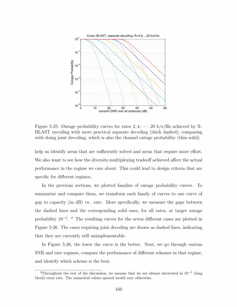
0 10 20 30 40 50 6010
−5
10−4
10−3
10−2
10−1
100
transmit SNR over all antennas (dB)
Out
age
Pro
babi
lity
Cross−BLAST, separate decoding, R=4,8,...,20 b/s/Hz
Figure 5-25: Outage probability curves for rates 2, 4, · · · , 20 b/s/Hz achieved by X-BLAST encoding with more practical separate decoding (thick dashed), comparingwith doing joint decoding, which is also the channel outage probability (thin solid).
help us identify areas that are sufficiently solved and areas that require more effort.
We also want to see how the diversity-multiplexing tradeoff achieved affect the actual
performance in the regime we care about. This could lead to design criteria that are
specific for different regimes.
In the previous sections, we plotted families of outage probability curves. To
summarize and compare them, we transform each family of curves to one curve of
gap to capacity (in dB) vs. rate. More specifically, we measure the gaps between
the dashed lines and the corresponding solid ones, for all rates, at target outage
probability 10−3. 4 The resulting curves for the seven different cases are plotted in
Figure 5-26. The cases requiring joint decoding are drawn as dashed lines, indicating
that they are currently still unimplementable.
In Figure 5-26, the lower the curve is the better. Next, we go through various
SNR and rate regimes, compare the performance of different schemes in that regime,
and identify which scheme is the best.
4Throughout the rest of the discussion, we assume that we are always interested in 10−3 (longblock) error rate. The numerical values quoted would vary otherwise.
160
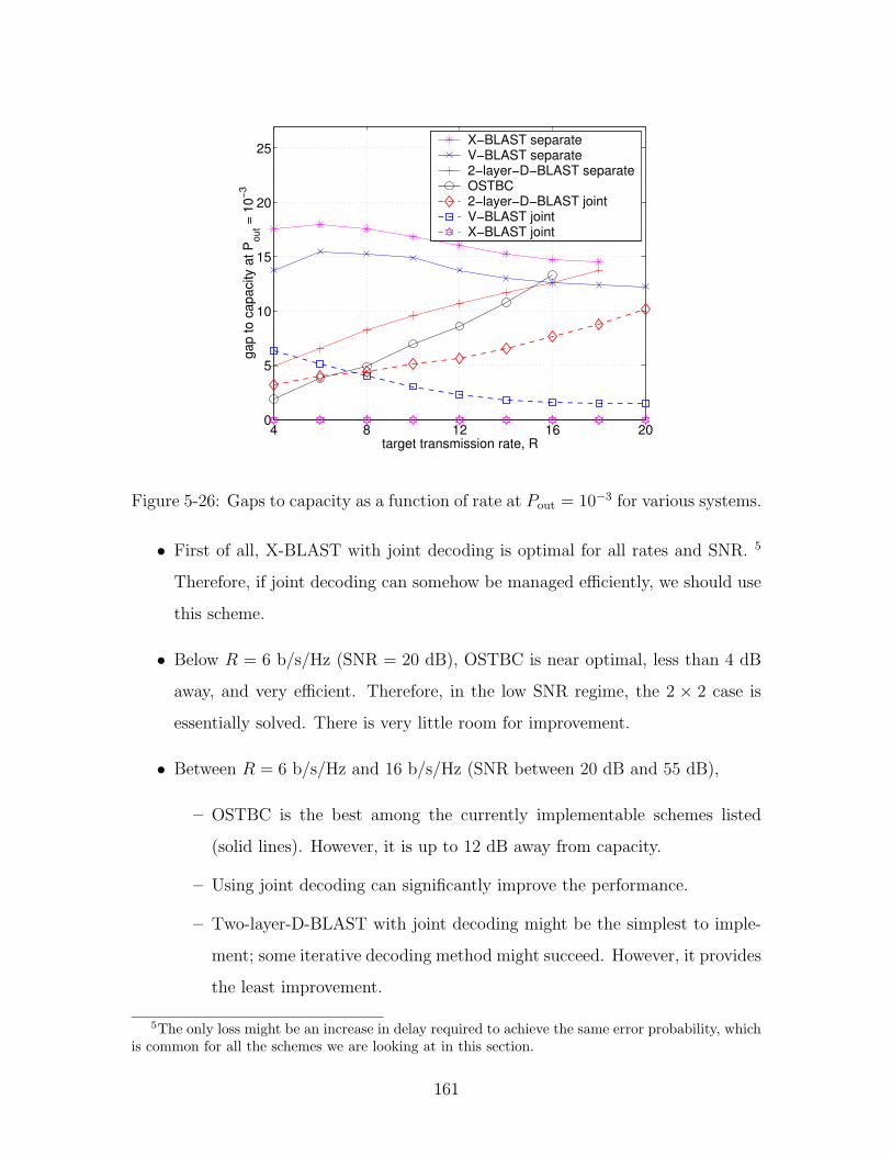
4 8 12 16 200
5
10
15
20
25
target transmission rate, R
gap
to c
apac
ity a
t Pou
t = 1
0−3
X−BLAST separateV−BLAST separate2−layer−D−BLAST separateOSTBC2−layer−D−BLAST jointV−BLAST jointX−BLAST joint
Figure 5-26: Gaps to capacity as a function of rate at Pout = 10−3 for various systems.
• First of all, X-BLAST with joint decoding is optimal for all rates and SNR. 5
Therefore, if joint decoding can somehow be managed efficiently, we should use
this scheme.
• Below R = 6 b/s/Hz (SNR = 20 dB), OSTBC is near optimal, less than 4 dB
away, and very efficient. Therefore, in the low SNR regime, the 2 × 2 case is
essentially solved. There is very little room for improvement.
• Between R = 6 b/s/Hz and 16 b/s/Hz (SNR between 20 dB and 55 dB),
– OSTBC is the best among the currently implementable schemes listed
(solid lines). However, it is up to 12 dB away from capacity.
– Using joint decoding can significantly improve the performance.
– Two-layer-D-BLAST with joint decoding might be the simplest to imple-
ment; some iterative decoding method might succeed. However, it provides
the least improvement.
5The only loss might be an increase in delay required to achieve the same error probability, whichis common for all the schemes we are looking at in this section.
161
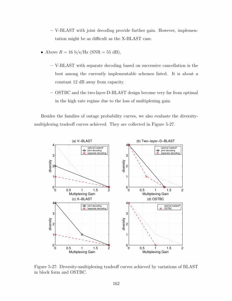
– V-BLAST with joint decoding provide further gain. However, implemen-
tation might be as difficult as the X-BLAST case.
• Above R = 16 b/s/Hz (SNR = 55 dB),
– V-BLAST with separate decoding based on successive cancellation is the
best among the currently implementable schemes listed. It is about a
constant 12 dB away from capacity.
– OSTBC and the two-layer-D-BLAST design become very far from optimal
in the high rate regime due to the loss of multiplexing gain.
Besides the families of outage probability curves, we also evaluate the diversity-
multiplexing tradeoff curves achieved. They are collected in Figure 5-27.
0 0.5 1 1.5 20
1
2
3
4
Multiplexing Gain
dive
rsity
(a) V−BLAST
optimal tradeoffjoint decodingseparate decoding
0 0.5 1 1.5 20
1
2
3
4
Multiplexing Gain
dive
rsity
(b) Two−layer−D−BLAST
optimal tradeoffjoint decodingseparate decoding
0 0.5 1 1.5 20
1
2
3
4
Multiplexing Gain
dive
rsity
(c) X−BLAST
joint decodingseparate decoding
0 0.5 1 1.5 20
1
2
3
4
Multiplexing Gain
dive
rsity
(d) OSTBC
optimal tradeoffOSTBC
Figure 5-27: Diversity-multiplexing tradeoff curves achieved by variations of BLASTin block form and OSTBC.
162
When joint decoding is used (solid curves), X-BLAST achieves the optimal trade-
off, V-BLAST achieves only the lower segment of the optimal tradeoff, while two-layer-
D-BLAST achieves only the upper segment. With separate decoding, X-BLAST and
V-BLAST achieves only the maximum multiplexing gain point, while two-layer-D-
BLAST and OSTBC achieves only the maximum diversity gain point.
Looking at Figure 5-26 and Figure 5-27 together, we can get some ideas of how
diversity-multiplexing tradeoff achieved can affect the actual performance in the
regime we care about. This could lead to design criteria that are specific for dif-
ferent regimes.
In the low SNR, low rate regime, it seems that achieving the maximum diversity
gain is important. This can be realized by the design criterion of maximizing the
worst case determinant, or at least keeping it away from zero.
In the high SNR, high rate regime (high relative to a certain target error rate),
it appears that achieving the maximum multiplexing gain is important, so that the
SNR required would grow with rate as slowly as possible. This can be realized by
utilizing all degrees of freedom and not using repetition. Comparing V-BLAST with
joint and with separate decoding, we see that it is much more advantageous to achieve
the entire lower segment of the tradeoff curve. The design criterion for this is still
unclear.
In the next two sections, we explore a couple schemes that actually employ joint
decoding, instead of successive cancellation based separate decoding. In particular,
we look at systems where tilted-QAM codes proposed in section 4.3 are combined
with hard-decision and soft-decision based error correction codes.
5.5 Tilted-QAM With Hard-Decision ECC
In this section, we build upon the tilted-QAM code we developed earlier in Chapter 4,
which achieves the optimal diversity-multiplexing tradeoff, and will strengthen it with
powerful error correction coding to obtain additional coding gain. In particular,
we concatenate it with a Reed-Solomon (RS) outer code with hard-decision based
163
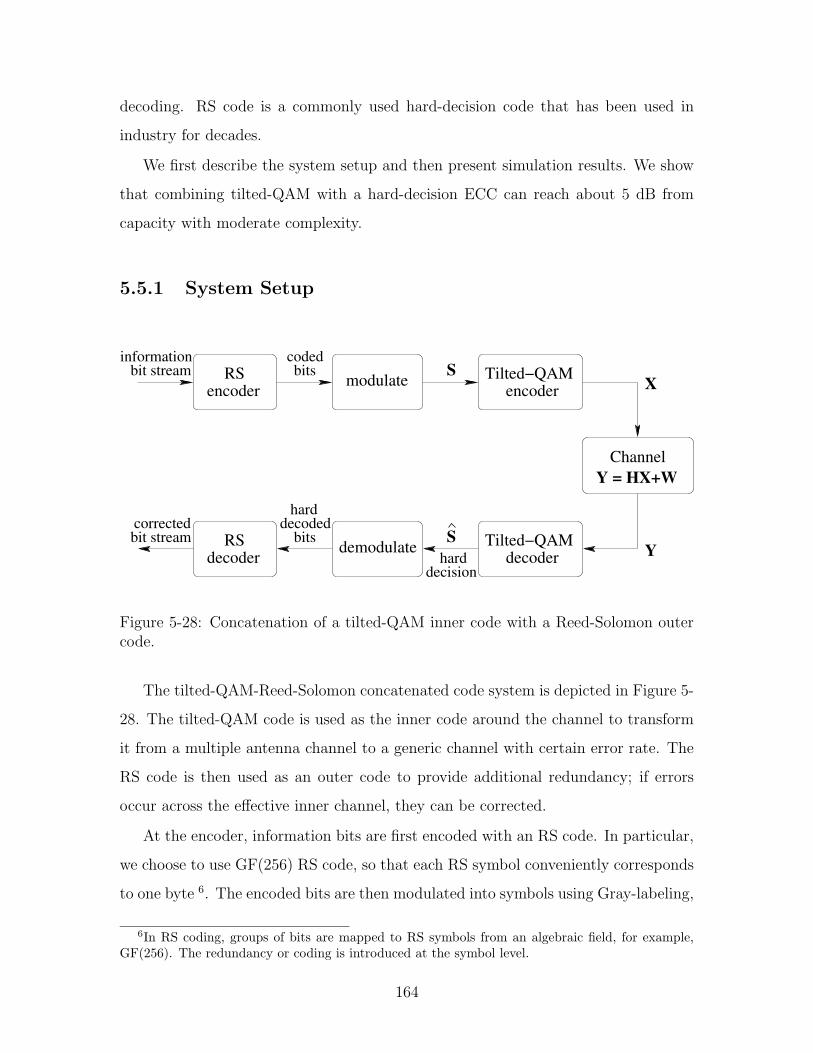
decoding. RS code is a commonly used hard-decision code that has been used in
industry for decades.
We first describe the system setup and then present simulation results. We show
that combining tilted-QAM with a hard-decision ECC can reach about 5 dB from
capacity with moderate complexity.
5.5.1 System Setup
Y = HX+WChannel
X
Ydecoder
encoder
RS
RS
demodulate
modulateS
S
encoderTilted−QAM
Tilted−QAMdecoderhard
bit streaminformation
bitscoded
bit streamcorrected
bitsdecoded
hard
decision
Figure 5-28: Concatenation of a tilted-QAM inner code with a Reed-Solomon outercode.
The tilted-QAM-Reed-Solomon concatenated code system is depicted in Figure 5-
28. The tilted-QAM code is used as the inner code around the channel to transform
it from a multiple antenna channel to a generic channel with certain error rate. The
RS code is then used as an outer code to provide additional redundancy; if errors
occur across the effective inner channel, they can be corrected.
At the encoder, information bits are first encoded with an RS code. In particular,
we choose to use GF(256) RS code, so that each RS symbol conveniently corresponds
to one byte 6. The encoded bits are then modulated into symbols using Gray-labeling,
6In RS coding, groups of bits are mapped to RS symbols from an algebraic field, for example,GF(256). The redundancy or coding is introduced at the symbol level.
164
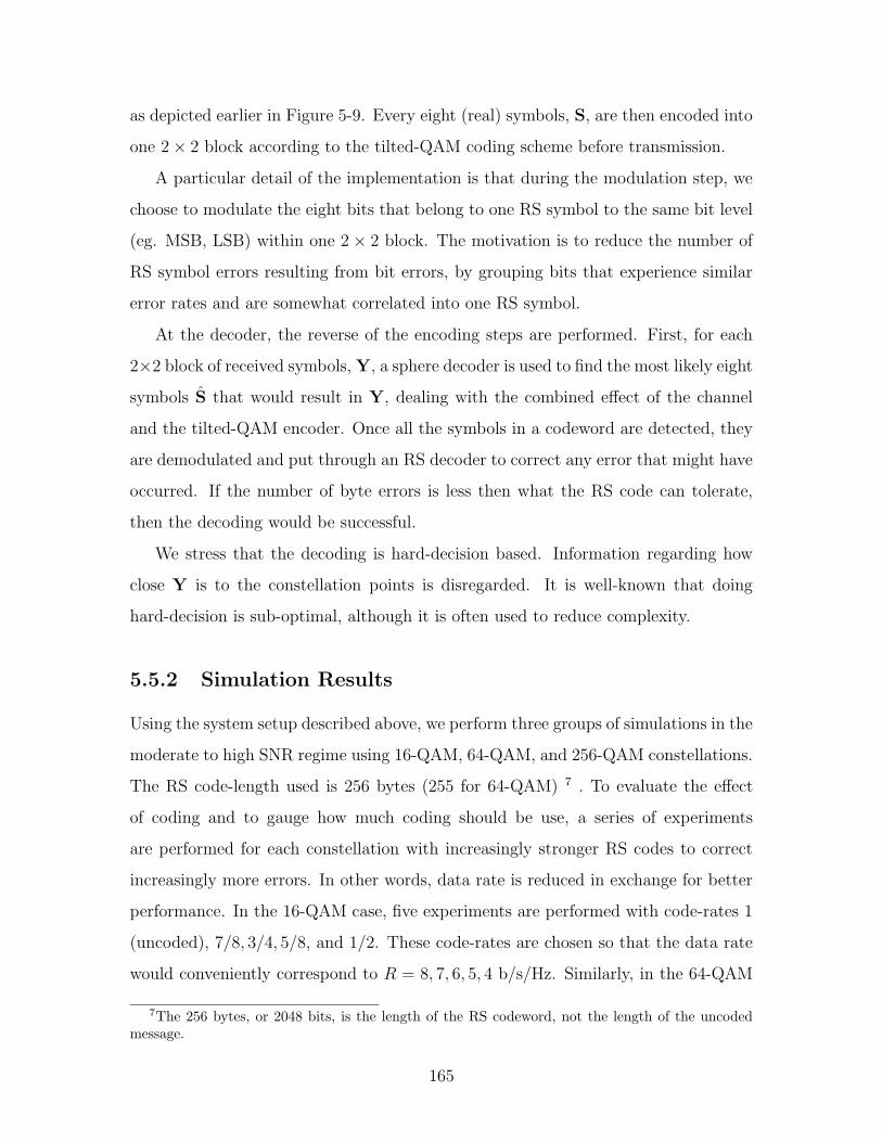
as depicted earlier in Figure 5-9. Every eight (real) symbols, S, are then encoded into
one 2× 2 block according to the tilted-QAM coding scheme before transmission.
A particular detail of the implementation is that during the modulation step, we
choose to modulate the eight bits that belong to one RS symbol to the same bit level
(eg. MSB, LSB) within one 2× 2 block. The motivation is to reduce the number of
RS symbol errors resulting from bit errors, by grouping bits that experience similar
error rates and are somewhat correlated into one RS symbol.
At the decoder, the reverse of the encoding steps are performed. First, for each
2×2 block of received symbols,Y, a sphere decoder is used to find the most likely eight
symbols S that would result in Y, dealing with the combined effect of the channel
and the tilted-QAM encoder. Once all the symbols in a codeword are detected, they
are demodulated and put through an RS decoder to correct any error that might have
occurred. If the number of byte errors is less then what the RS code can tolerate,
then the decoding would be successful.
We stress that the decoding is hard-decision based. Information regarding how
close Y is to the constellation points is disregarded. It is well-known that doing
hard-decision is sub-optimal, although it is often used to reduce complexity.
5.5.2 Simulation Results
Using the system setup described above, we perform three groups of simulations in the
moderate to high SNR regime using 16-QAM, 64-QAM, and 256-QAM constellations.
The RS code-length used is 256 bytes (255 for 64-QAM) 7 . To evaluate the effect
of coding and to gauge how much coding should be use, a series of experiments
are performed for each constellation with increasingly stronger RS codes to correct
increasingly more errors. In other words, data rate is reduced in exchange for better
performance. In the 16-QAM case, five experiments are performed with code-rates 1
(uncoded), 7/8, 3/4, 5/8, and 1/2. These code-rates are chosen so that the data rate
would conveniently correspond to R = 8, 7, 6, 5, 4 b/s/Hz. Similarly, in the 64-QAM
7The 256 bytes, or 2048 bits, is the length of the RS codeword, not the length of the uncodedmessage.
165
case, seven experiments are run with R = 12, 11, · · · , 6 b/s/Hz; in the 256-QAM case,
there are nine experiments with R = 16, 15, · · · , 8 b/s/Hz.
The resulting block error rate curves are shown in Figure 5-29. The three groups
of experiments can be identified by the different SNR intervals and the experiments
within the groups are selectively labeled by the rates R.
18 20 22 24 26 28 30 32 34 36 38 40
10−3
10−2
10−1
100
total transmit SNR in dB
256
byte
s bl
ock
erro
r rat
e
64−QAM 256−QAM16−QAM
R=8
R=7
R=4
R=12
R=11
R=6 R=8
R=15
R=16
Figure 5-29: Block error rate curves for 16-QAM, 64-QAM, and 256-QAM cases. Aswe gradually reduce the data rate by 1 b/s/Hz, the block error rate lowers due tostronger coding. However, the gain diminishes.
We see that for each of the three groups of curves, the top gap is always the largest,
which corresponds to the greatest improvement in block error rate for 1 bit of rate
reduction. As we reduce the rate further, although the block error rate improves, the
gain diminishes. The reason for the diminishing gain is that we are operating in the
regime where the uncoded error rate is not too high. Although there are often some
errors to be corrected, most of those times, there are only a few errors. It becomes
less likely to have more.
In conclusion, it appears that a small amount of coding is sufficient, about 1
b/s/Hz rate reduction. If we apply too much coding, then the gain from correcting a
few more block errors would not be worth the reduction in rate, or the constellation
166
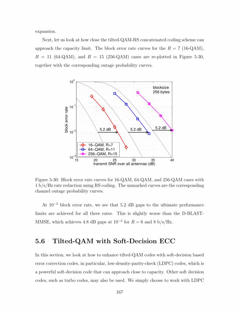
expansion.
Next, let us look at how close the tilted-QAM-RS concatenated coding scheme can
approach the capacity limit. The block error rate curves for the R = 7 (16-QAM),
R = 11 (64-QAM), and R = 15 (256-QAM) cases are re-plotted in Figure 5-30,
together with the corresponding outage probability curves.
15 20 25 30 35 4010
−3
10−2
10−1
100
transmit SNR over all antennas (dB)
bloc
k er
ror r
ate
blocksize256 bytes
5.2 dB 5.2 dB 5.2 dB
16−QAM, R=764−QAM, R=11256−QAM, R=15
Figure 5-30: Block error rate curves for 16-QAM, 64-QAM, and 256-QAM cases with1 b/s/Hz rate reduction using RS coding. The unmarked curves are the correspondingchannel outage probability curves.
At 10−2 block error rate, we see that 5.2 dB gaps to the ultimate performance
limits are achieved for all three rates. This is slightly worse than the D-BLAST-
MMSE, which achieves 4.8 dB gaps at 10−2 for R = 6 and 8 b/s/Hz.
5.6 Tilted-QAM with Soft-Decision ECC
In this section, we look at how to enhance tilted-QAM codes with soft-decision based
error correction codes, in particular, low-density-parity-check (LDPC) codes, which is
a powerful soft-decision code that can approach close to capacity. Other soft decision
codes, such as turbo codes, may also be used. We simply choose to work with LDPC
167
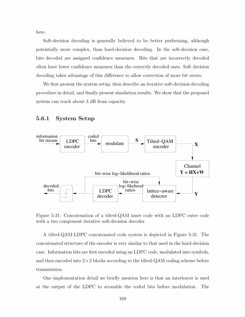
here.
Soft-decision decoding is generally believed to be better performing, although
potentially more complex, than hard-decision decoding. In the soft-decision case,
bits decoded are assigned confidence measures. Bits that are incorrectly decoded
often have lower confidence measures than the correctly decoded ones. Soft decision
decoding takes advantage of this difference to allow correction of more bit errors.
We first present the system setup, then describe an iterative soft-decision decoding
procedure in detail, and finally present simulation results. We show that the proposed
system can reach about 3 dB from capacity.
5.6.1 System Setup
Y = HX+WChannel
decoderLDPC
X
Y
encodermodulate
Sencoder
Tilted−QAMLDPC
detectorlattice−awarebits ratios
bit streaminformation
bitscoded
bit−wise log−likelihood ratios
log−likehoodbit−wise
decoded
Figure 5-31: Concatenation of a tilted-QAM inner code with an LDPC outer codewith a two component iterative soft-decision decoder.
A tilted-QAM-LDPC concatenated code system is depicted in Figure 5-31. The
concatenated structure of the encoder is very similar to that used in the hard-decision
case. Information bits are first encoded using an LDPC code, modulated into symbols,
and then encoded into 2×2 blocks according to the tilted-QAM coding scheme before
transmission.
One implementation detail we briefly mention here is that an interleaver is used
at the output of the LDPC to scramble the coded bits before modulation. The
168
motivation is that bits modulated within the same 2 × 2 tilted-QAM coded matrix
suffer correlated errors. We want those bits to be well separated within a codeword.
For brevity, the interleaver and de-interleaver are not shown explicitly in Figure 5-31.
At the receiver, a two-component iterative soft-decision decoder is used. Tentative
decisions of the bits expressed as log-likelihood-ratios (LLR) are passed iteratively
between a lattice-aware detector and an LDPC decoder until convergence or until a
maximum number of iterations is reached. Afterward, the decisions are finalized by
comparing the LLRs to a threshold, typically zero. The details of this decoder will
be described shortly.
The motivation for the two-component and iterative structure is that the two
components each handles a particular aspect of the decoding. The lattice-aware
detector deals with the channel distortion and the lattice structure of the tilted-
QAM code, and knows what symbols are close to the received point; while the LDPC
decoder focus on the redundancy, and knows which bit strings are valid codewords.
For optimal decoding, both aspects should be considered simultaneously, i.e., we want
a valid codeword that is the closest to the received point. However, directly solving
for it would have extremely high complexity. Instead, we iterate between the two
components, allow them to exchange information and come to a joint conclusion as
their decisions converge.
Next, we describe the iterative soft-decision decoding algorithm in detail.
5.6.2 Iterative Soft-Decision Decoder
The detail of the iterative soft-decision decoder is shown in Figure 5-32. The log-
likelihood-ratio scores passed between the LDPC decoder and the lattice-aware de-
tector are labeled. These forms of LLR are common to many soft-decision systems.
Let us first look at the LDPC decoder. We do not say much about it here except
that the input bit-wise LLR scores it requires are
logP [Y|b = 1]
P [Y|b = 0], (5.43)
169
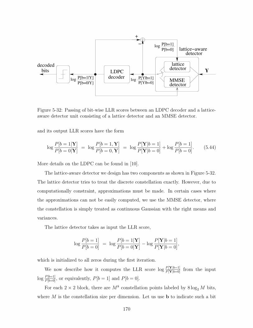
decoderLDPC
P[Y|b=1]P[Y|b=0]
log
decodedbits
P[b=1|Y]P[b=0|Y]
log
P[b=1]P[b=0]
log
+
Y
−
detectorMMSE
detectorlattice
detectorlattice−aware
Figure 5-32: Passing of bit-wise LLR scores between an LDPC decoder and a lattice-aware detector unit consisting of a lattice detector and an MMSE detector.
and its output LLR scores have the form
logP [b = 1|Y]
P [b = 0|Y]= log
P [b = 1,Y]
P [b = 0,Y]= log
P [Y|b = 1]
P [Y|b = 0]+ log
P [b = 1]
P [b = 0]. (5.44)
More details on the LDPC can be found in [10].
The lattice-aware detector we design has two components as shown in Figure 5-32.
The lattice detector tries to treat the discrete constellation exactly. However, due to
computationally constraint, approximations must be made. In certain cases where
the approximations can not be easily computed, we use the MMSE detector, where
the constellation is simply treated as continuous Gaussian with the right means and
variances.
The lattice detector takes as input the LLR score,
logP [b = 1]
P [b = 0]= log
P [b = 1|Y]
P [b = 0|Y]− log
P [Y|b = 1]
P [Y|b = 0],
which is initialized to all zeros during the first iteration.
We now describe how it computes the LLR score log P [Y|b=1]P [Y|b=0] from the input
log P [b=1]P [b=0]
, or equivalently, P [b = 1] and P [b = 0].
For each 2 × 2 block, there are M 8 constellation points labeled by 8 log2M bits,
where M is the constellation size per dimension. Let us use b to indicate such a bit
170
string, and use bi for the ith bit, then we have
logP [Y|bi = 1]
P [Y|bi = 0]= log
P [bi = 1,Y]
P [bi = 0,Y]− log
P [bi = 1]
P [bi = 0](5.45)
= log
∑b|bi=1 P [Y|b] · P [b]
∑b|bi=0 P [Y|b] · P [b]
− logP [bi = 1]
P [bi = 0]. (5.46)
To compute P [b], the bits are treated as if they were independent, i.e.,
P [b] =
8 log2M∏
j=1
P [bj].
This is because the redundancy is ignored by the lattice detector and is only handled
by the LDPC decoder.
The conditional probability P [Y|b] is
P [Y|b] ∝ exp
‖Y −HX(b)‖22σ2w
,
whereX(b) is the transmit constellation point corresponding to the bit string b. This
is a result of the additive white Gaussian noise assumption.
To compute log P [Y|bi=1]P [Y|bi=0] exactly according to (5.46), we need to sum over all
M8 constellation points. However, this is obviously too computationally intensive.
Instead, we approximate it by listing a small number of points with the highest values
of P [Y|b]P [b] and only summing over them. Similar listing technique was used by
Hochwald and ten Brink in [14].
To determine the number of points to list, we must find a balance between com-
plexity and performance. We should list as few as possible to keep the complexity
low, and list as many as possible so that the approximation is good. In our simula-
tions, we choose to use 40 ∼ 120 points, which has acceptable complexity, and seem
to yield reasonably good performance.
Listing the set of constellation points with the highest values of P [Y|b]P [b] is
done using a specially modified sphere decoder. We will not discuss sphere decoder
in detail here except that it locates the closest point in a high dimensional lattice to
171
a given point. We modify the sphere decoder to list all the points within a certain
radius. We also modified it to consider 2σ2w log(P [b])+‖Y−HX(b)‖2 as the effectivedistance measure, so that the likelihood scores are included.
Once we have the list of points with the highest values of P [Y|b]P [b], we can
then perform the summation in (5.46) over this set for each bit bi. From this, the
lattice detector can compute its output LLR scores.
The LLR scores computed using the partial sum approximation are good in many
cases; however, for some bits, the points listed might all have that bit being 1 or
all 0. When this happens, one of the summations in (5.46) would be empty, and
no meaningful LLR score can be computed. This would typically happen for MSBs,
since points with different MSBs are often far away. For these bits, we use the MMSE
detector.
We perform MMSE detection for each symbol in S treating all others as continuous
interference. Once we obtain the MMSE estimate, we can consider the equivalent
channel, s = s+e, and compute LLR scores for each bit in the symbol using the same
method as in the D-BLAST-MMSE case (see Figure. 5-10).
As iterations go by, we can use existing soft estimates of the bits in the form of
log P [b=1|Y]P [b=0|Y]
to help reduce the interference. We estimate the mean of the interference
and cancel that out. Eventually, if all the bits are known exactly, then there would be
no interference left. We choose to use log P [b=1|Y]P [b=0|Y]
instead of log P [b=1]P [b=0]
because it carries
more information about the bits and seem to yield better performance empirically.
Combining the lattice detector and the MMSE detector, LLR scores for all bits
can be computed.
Note that the main difference between the lattice detector and the MMSE detector
is that the former treats the interference as discrete while the latter treats it as
continuous. Given a certain received signal point, it is important to treat the nearby
points as discrete to have accurate measures of the distances to them, which is done
by the lattice detector. For points far away however, the discreteness matters less,
allowing us to use the MMSE detector.
172
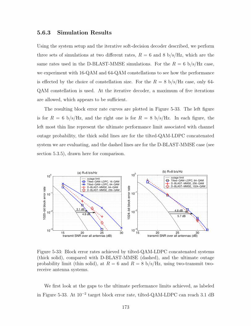
5.6.3 Simulation Results
Using the system setup and the iterative soft-decision decoder described, we perform
three sets of simulations at two different rates, R = 6 and 8 b/s/Hz, which are the
same rates used in the D-BLAST-MMSE simulations. For the R = 6 b/s/Hz case,
we experiment with 16-QAM and 64-QAM constellations to see how the performance
is effected by the choice of constellation size. For the R = 8 b/s/Hz case, only 64-
QAM constellation is used. At the iterative decoder, a maximum of five iterations
are allowed, which appears to be sufficient.
The resulting block error rate curves are plotted in Figure 5-33. The left figure
is for R = 6 b/s/Hz, and the right one is for R = 8 b/s/Hz. In each figure, the
left most thin line represent the ultimate performance limit associated with channel
outage probability, the thick solid lines are for the tilted-QAM-LDPC concatenated
system we are evaluating, and the dashed lines are for the D-BLAST-MMSE case (see
section 5.3.5), drawn here for comparison.
15 20 25 3010−3
10−2
10−1
100
transmit SNR over all antennas (dB)
1020
−bit
bloc
k er
ror r
ate
(a) R=6 b/s/Hz
3.1 dB
4.8 dB
outage limitTilted−QAM−LDPC, 16−QAMTilted−QAM−LDPC, 64−QAMD−BLAST−MMSE, 64−QAMD−BLAST−MMSE, 256−QAM
15 20 25 3010−3
10−2
10−1
100
transmit SNR over all antennas (dB)
1024
−bit
bloc
k er
ror r
ate
(b) R=8 b/s/Hz
4.8 dB
5.7 dB
outage limitTilted−QAM−LDPC, 64−QAMD−BLAST−MMSE, 256−QAMD−BLAST−MMSE, 1024−QAM
Figure 5-33: Block error rates achieved by tilted-QAM-LDPC concatenated systems(thick solid), compared with D-BLAST-MMSE (dashed), and the ultimate outageprobability limit (thin solid), at R = 6 and R = 8 b/s/Hz, using two-transmit two-receive antenna systems.
We first look at the gaps to the ultimate performance limits achieved, as labeled
in Figure 5-33. At 10−2 target block error rate, tilted-QAM-LDPC can reach 3.1 dB
173
from capacity in the R = 6 b/s/Hz case. Compared to D-BLAST-MMSE, which
is 4.8 dB away, a small improvement in performance is achieved. This is because
D-BLAST-MMSE treats the interference between the symbols as Gaussian, when it
is really discrete. (This problem was discussed earlier in section 5.3.3.) Tilted-QAM-
LDPC, on the other hand, avoids this problem using the lattice-aware detector.
In the R = 8 b/s/Hz case, tilted-QAM-LDPC only reaches 5.7 dB from capacity,
and is about 1 dB worse than D-BLAST-MMSE, which is still 4.8 dB away. The
reason for this degradation in performance is that, as rate increases, it becomes more
difficult to perform the soft-decision decoding. In particular, the lattice detector only
considers a small number of neighbors instead of all the constellation points to reduce
complexity. The larger the constellation is, the worse the approximation.
We note that in all the experiments performed, no constellation shaping is used.
Therefore, all the gaps to capacity quoted include a portion due to the lack of shaping
gain. With simple shaping techniques, the resulting gap could be smaller by about
1 dB.
Next, let us turn our attention to the constellation size issue. Compare the two
tilted-QAM-LDPC results (thick solid lines) in the R = 6 b/s/Hz case, it is clear
that 16-QAM constellation does better than 64-QAM. This is because when the con-
stellation is unnecessarily dense, the points become too close compared to the noise
level. When this happens, noise could carry the original signal to many constellation
points away, and the transmitted point would not be among the nearby neighbors of
the received point, and would not be considered by the lattice detector.
Another constellation size issue worth noting is that tilted-QAM-LDPC uses
much smaller constellations compared to D-BLAST-MMSE, while achieving simi-
lar performance. Smaller constellations are preferred for ease of implementation.
For R = 6 b/s/Hz, tilted-QAM-LDPC uses 16-QAM constellation, while D-BLAST-
MMSE uses 256-QAM. This is due to the finite constellation problem of D-BLAST
we discussed in section 5.3.3. As tilted-QAM-LDPC demonstrates, this problem is
avoidable.
174

5.7 Summary
In this chapter, we study building practical system using long error correction codes
in the multiple antenna communication scenario. We combine powerful coding tech-
niques developed for scalar AWGN channels with multiple antenna coding techniques,
in particular, OSTBC, various versions of BLAST, and tilted-QAM codes.
We examine two approaches. One is to transform a multiple antenna channel to
multiple single antenna channels. This leads to application of error correction codes
in a natural way. This is the approach taken by various versions of BLAST with
successive cancellation decoding. The other approach is to use a concatenated coding
scheme where codes specific to the multiple antenna channel, such as tilted-QAM
codes, are used as inner codes, and hard or soft-decision ECC are used outer codes to
further enhance the performance of the overall system. A system combining OSTBC
and ECC can be interpreted both ways.
We show that OSTBC enhanced with capacity achieving ECC is near optimal
in the low SNR regime. It is less than 1 dB from optimal for SNR below 10 dB
and rate below 2 b/s/Hz and less than 3 dB from optimal for SNR below 20 dB
and rate below 6 b/s/Hz. This suggests that although OSTBC loses multiplexing
gain due to repetition, it is still a very attractive method in the low SNR regime. It
also has very simple implementation and low decoding complexity. However, OSTBC
becomes increasingly sub-optimal in the high SNR regime. Also, there is no good
higher-dimensional OSTBC codes for systems with more than two antennas.
While OSTBC can be used for systems operating in low to moderate SNR regimes,
coding schemes suitable for high SNR still needs further study. Current designs like
diagonal-BLAST is theoretically optimal, but its non-block form leads to practical
problems like error propagation. Other block form variations like V-BLAST and X-
BLAST would be optimal or close to being optimal if joint decoding can be done.
However, there is no efficient joint decoding scheme at this time.
We experiment with combining tilted-QAM code with hard and soft decision error
correction codes. The complexity of the joint decoding involved is feasible for off-line
175
simulations but beyond reach for current real time systems, especially in the case
of soft decoding. At the target error rate of 10−2, the resulting gap to capacity is
about 5.2 dB for hard decision systems. For soft-decision ones, the gap is 3.1 dB for
R = 6 b/s/Hz and 5.7 dB for R = 8 b/s/Hz. In comparison, D-BLAST-MMSE is
4.8 dB from capacity at those rates.
From our study, it is evident that more work is needed to design good systems for
multiple antenna communication in the high SNR regime and using more antennas,
and new design criteria might be needed.
176
Chapter 6
Non-Coherent Communications
In the earlier chapters, we have assumed perfect channel knowledge at the receiver.
However, in many practical applications, this assumption can not be satisfied exactly.
For example, the channel might be varying too fast to be tracked accurately. This
scenario is appearing more and more often as wireless devices are now operating at
higher and higher carrier frequencies while the lower frequency spectrum becomes
quickly filled. Even when the channel is varying more slowly, we might only be able
to track it to some degree, instead of having perfect channel knowledge.
In this chapter, we investigate the case of non-coherent communication, where
the channel knowledge at the receiver is absent or imperfect. Again, we assume that
the transmitter has no channel knowledge. We continue to model the channel as
Y = HX+W, where the Nr ×Nt, Nr ≥ Nt, matrix H represents the flat, Rayleigh,
and block fading channel, andW is the additive white Gaussian noise. Entries of H
and W are independent with identical distribution CN(0, 1). The average energy of
each entry of X is ρ, while that of each column of X is SNR = Ntρ.
There are still many unanswered question for this non-coherent communication
problem. Neither exact capacity formulas nor efficient encoding and decoding algo-
rithms exist. Only some aspects of the achievable capacity are known and there exist
some inefficient or sub-optimal coding algorithms.
We first review some existing work on theoretical results, design rules, as well as
some specific designs. Then, we propose a geometric approach that links the non-
177
coherent signal design problem to that of the coherent case with training, where some
predetermined, non-information bearing signal is sent to probe the channel. We argue
that the training approach is not too far from being optimal. We also look at what
decoding performance can be achieved using the channel estimates obtained through
training.
6.1 Theoretical Background
6.1.1 Capacity
The capacity of a non-coherent system is clearly upper bounded by the capacity of
a system where the channel coefficients are perfectly known by the receiver, which is
[36]
Cu = log2(det(INr
+ ρHH†)), (6.1)
where ρ = SNR/Nt is the average transmit SNR per antenna.
This capacity grows linearly with log2 ρ in the limit of high SNR. Specifically, for
every 3 dB increase in SNR, the capacity grows byK b/s/Hz, whereK = min(Nt, Nr).
For non-coherent systems, it turns out that the growth rate is slightly modified.
Zheng and Tse studied the capacity of non-coherent systems in the limit of
high SNR, assuming block fading model in [40]. They showed that non-coherent
capacity also grows linearly in the limit of high SNR. The difference is that for
every 3 dB increase in SNR, the capacity grows by K(1 − K/T ) b/s/Hz, where
K = min(Nt, Nr, bT/2c) and T is the coherence time of the channel, which is the
time that the channel remains constant before independently changing to other val-
ues.
While the full proof is more involved, the intuition behind the capacity growth
rate result is a dimensionality count. For simplicity, let us look at the symmetric
case, K = Nt = Nr ≤ T/2. At the transmitter, with K transmit antennas and
a block of T times, we have KT degrees of freedom. At the receiver, we need to
178
solve for the channel, which has NtNr = K2 degrees of freedom. So we are left with
KT −K2 = K(T −K) degrees of freedom for transmitting information. Normalize
this by time, we have K(1−K/T ).
Furthermore, [42] shows that a non-coherent system with Nt transmit antennas 1,
Nr receive antennas, and block length T , has similar diversity-multiplexing tradeoff
as a coherent system with the same number of antennas and block length T − Nt.
The difference is that the tradeoff curved achieved is scaled in the direction of the
multiplexing gain, the r axis, by a factor of (1−Nt/T ). This tradeoff can be achieved
with training, where a pilot signal of duration Nt is first sent to allow the receiver to
learn the channel and then the system is treated as coherent. The training phase is
what causes the reduction of the factor of (1−Nt/T ) in multiplexing gain. In the limit
of T →∞, or slow fading, (1−Nt/T ) approaches 1. The non-coherent capacity meets
the perfect-knowledge upper bound as expected. Since for large coherence time, we
can spend some time to learn the channel first with negligible cost in rate.
One crucial assumption made in [42] is that the channel stays constant exactly
during the coherence time of the channel, so that we can learn the channel to any
precision desired and then treat the channel as known. However, this block fading
model is not accurate. In reality, channel varies continuously, so that future channel
coefficients can be estimated, but not perfectly. In [16], Lapidoth and Moser modeled
the channel as jointly stationary and ergodic stochastic processes. They concluded
that at high SNR, capacity grows double-logarithmically in SNR and not logarithmi-
cally as in the block fading case. They suggested in [17] that this double-logarithmic
behavior is dominant when the transmission rate significantly exceeds a fading num-
ber, which is typically increased by using multiple antennas. At this point, let us
assume that the regime we are interested in is below this fading number, so that the
block fading model is still reasonably good.
1Assume all Nt transmit antennas are used in this statement. Sometimes, it is preferable not touse all antennas available.
179
6.1.2 Capacity Achieving Distribution
In order to design good coding schemes, we first look at the capacity achieving distri-
bution, which was studied in [24]. Given a particular distribution on the transmitted
signal matrix X, the mutual information between the input and output of the channel
is defined as,
I(Y;X) = EY,X
[log
(p(Y|X)
EY[p(Y|X)]
)]. (6.2)
The capacity achieving distribution is the distribution p(X) that maximizes the mu-
tual information to achieve capacity,
C = supp(X)
I(Y;X). (6.3)
The mutual information I(Y;X) is a function of both p(Y|X) and p(X). There-
fore, the distribution p(X) that maximizes I(Y;X) depends on p(Y|X), which we
now look at. In the case of Y = HX+W, where the entries of H and W are IID
CN(0, 1) random variables, and X is Nt × T , we have
p(Y|X) =exp
(−tr
((IT +X†X
)−1Y†Y
))
πTNr(det (IT +X†X))Nr. (6.4)
We see that the effect of X appears only through X†X, so we can multiply X by any
unitary matrix on the left without changing p(Y|X). We can perform singular value
decomposition on X and factor it into X = ΨΛΦ†, where Ψ and Φ are unitary and Λ
is diagonal. Since we can remove Ψ by multiplying Ψ† on the left without changing
p(Y|X), we can limit X to take the form of just X = ΛΦ† with no loss of generality.
With some additional rotational symmetry argument, it turns out that the capacity
distribution is given by the following lemma [24].
Lemma 6.1 The signal matrix that achieves capacity can always be factored as
X = ΛΦ†, where Φ is an T ×Nt isotropically distributed unitary matrix, and Λ is an
independent Nt ×Nt real, non-negative, diagonal matrix.
180
An isotropically distributed unit vector is a unit length vector that is equally
likely to point in any direction. An isotropically distributed unitary matrix is a
matrix whose columns are isotropically distributed unit vectors that also satisfy the
orthogonality constraint, i.e., the second column is a vector that is equally likely to
point in any direction that is orthogonal to the first, and so on. One property of
isotropically distributed unitary matrix is rotational symmetry, i.e., p(Φ) = p(ΘΦ),
for any unitary matrix Θ.
The capacity achieving distribution for the diagonal matrix Λ is not given in [24]
except in the limiting case. For fixed Nt, as T → ∞, the optimal distribution of Λ
converges to√ρT INt
in probability. This means that when T is large enough, we
can pick all diagonal entries of Λ to be√ρT , so that, X =
√ρTΦ†. For the case of
Nt = Nr = 1, this approximation is shown to be good when T > 12 at SNR = 0 dB,
T > 4 at SNR = 6 dB, and T > 3 at SNR = 12 dB [24]. We see that the lengths
required are not very large and can be satisfied easily in practice.
It seems intuitive that the capacity achieving distribution should be isotropic when
the channel is Rayleigh fading and the transmitter has absolutely no knowledge of
the realized channel. However, if the transmitter were to have some side information
about the realized channel through feedback or if the channel were not Rayleigh
fading, then the symmetry would be broken and the capacity achieving distribution
would be different. Some of these issues are investigated in [37].
In comparison, the capacity achieving distribution for the AWGN channel is simply
Gaussian with zero mean and variance matching the signal power constraint. The
capacity achieving distribution of the non-coherent multiple antenna channel is much
more complicated, and the coding problem is more difficult as well.
6.2 Non-Coherent Communication Signal Design
By looking at the capacity achieving distribution, we have established that when
T is sufficiently large, we can pick the transmitted signal matrix for message l,
l ∈ 1, · · · , L, to be X =√ρTΦ†l , where Φl is an T × Nt unitary matrix and L
181
is the size of the signal set. This scheme is called Unitary Space-Time Modulation.
Geometrically, unitary matrices, or the subspaces they span, are used to represent
messages. In comparison, points are used for AWGN channels.
6.2.1 Design Criterion
In this study, the Nt× T transmitted signal matrix Φ is considered as one codeword,
and we are interested in detecting which one is transmitted from the received signal
Y =√ρTHΦ†l +W.
The maximum-likelihood detector for this signal set is ΦML = argmaxΦlp(Y|Φl).
After some mathematical manipulation, it turns out to be [12]
ΦML = argmaxΦl∈Φ1,··· ,ΦL
tr (YΦ†lΦlY†). (6.5)
This ML detector maximizes the energy contained in the product Yֆl , similar to
match filtering. With this detector, the pair-wise error probability, the probability of
confusing Φ1 and Φ2 while ignoring other ones, has a Chernoff upper bound of
P [Φ1 → Φ2] ≤1
2
Nt∏
n=1
[1
1 + (ρT/Nt)2(1−d2n)4(1+ρT/Nt)
]Nr
, (6.6)
where 1 ≥ d1 ≥ . . . ≥ dNt≥ 0 are the singular values of the Nt × Nt correlation
matrix Φ†2Φ1.
From the above equation, we see that the probability of error decreases with
decreasing dn. Geometrically, these dn′s correspond to the cosine’s of a set of principle
angles defined between the two subspaces spanned by Φ1 and Φ2. Therefore, to design
a good signal set that has low probability of error, we need to find a set of unitary
matrices, such that the subspaces they span are well separated in terms of the angles
between them.
182
6.2.2 Existing Schemes
Next, we review some existing signal design schemes.
Iterative Search Method One iterative method of searching for a good determin-
istic signal set was described in [12]. The basic idea is to start from an initial signal
set and improve it iteratively. We first compute all pairs of correlation matrices Φ†iΦj,
and then identify the worst pair and try to “move them apart”. This procedure is
repeated until improvement diminishes. This method is computationally intensive,
especially when the signal set is large. For a signal set of size L, there are L(L− 1)/2
pairs of correlations to compute. Therefore, this method is only applicable in low
dimensional and low rate cases.
Systematic Design of Unitary Space-Time Signals A systematic method of
designing good unitary space-time signal sets was developed in [13]. The design is not
optimal, but the design complexity is low. The idea is to design one unitary matrix
Θ and use it to generate all signal matrices in the set. More specifically, the design
proposed is
Φl = Θl−1Φ1, for l = 1, · · · , L, (6.7)
where Θ is a T × T unitary matrix such that ΘL = IT , and Φ1 is a T × Nt unitary
matrix. The advantage of this design is that, for any two Φi and Φj, the correlation is
Φ†1Θ((j−i) mod L)Φ1. Every signal matrix forms the same set of correlation matrices
with all the other signal matrices. Now there are only L − 1 correlation matrices to
check, instead of L(L− 1)/2. To further reduce the design complexity, Θ is restricted
to be diagonal with entries Θtt = ej(2π/L)ut for t = 1, · · · , T , where ut are integers
satisfying 0 ≤ u1 ≤ · · · ≤ uT ≤ L − 1. Now we only need to search over a finite set
of integers to find the best Θ.
Unitary Space-Time Autocoding Constellations Another structured way of
designing unitary space-time signal sets was proposed in [23]. A signal set of size
183
L = 2RT takes the form of
Φl1l2···lRT= Ωl1
1 Ωl22 · · ·ΩlRT
RT Φ00···0, l1, l2, · · · , lRT ∈ 0, 1, (6.8)
where Φ00···0 is T ×Nt and Ω1, · · ·ΩRT are T ×T independent isotropically distributed
unitary matrices. 2 A desirable property of this design is that, statistically, every sig-
nal set has signal matrices that are pair-wise independent and marginally isotropically
random. This statistics is capacity achieving.
Differential Coding Differential coding is well studied for the non-coherent single
antenna system, and was extended to multiple antenna systems by various groups
[11, 33]. In this case, Nt×Nt matrices are used to represent messages. The idea is to
utilize the fact that channel does not change much between these short blocks, and
transmit
Xτ = Xτ−1Φ†l (6.9)
for message l during block τ . This differential scheme leads to
Yτ = H(Xτ−1Φ†l ) +Wτ = Yτ−1Φ
†l + (Wτ −Wτ−1Φ
†l ). (6.10)
The effective channel is Yτ−1, which is perfectly known at the receiver. The detection
problem becomes a coherent one. However, the down-side is that the noise from
the previous block, Wτ−1, propagates through, so that the effective noise power is
doubled. Note that, for differential coding, the block fading model is not used.
2Detection for this signal set is like “trying to pick a combination lock”. There is no efficientalgorithm but exhaustive search.
184
6.3 Geometric Approach
The criterion for designing good codes for non-coherent communication is to have a
set of unitary matrices such that the subspaces they span are well separated in terms
of the angles between them. Most of the existing schemes design unitary matrices
algebraically. In this section, we introduce a geometric approach. This is based on
work by Conway and Sloane on packing low dimensional subspaces in high dimensions
[5].
6.3.1 Projection Matrices
Subspaces have a one-to-one relationship with projection matrices corresponding to
projection onto that subspace. A subspace spanned by a T × Nt unitary matrix
Φ corresponds to a T × T projection matrix P = ΦΦ† with rank Nt. The task of
designing good signal sets can be turned into choosing a set of projection matrices
that are well separated in terms of a Euclidean distance, which is a metric that we
are much more familiar with and can visualize easily.
The Euclidean distance between two matrices is defined as the L2 norm of the
difference matrices. Let P1 −P2 = ∆, and let δij be the entries of ∆,
‖P1 −P2‖2 = ‖∆‖2 =∑∑
δ2ij = tr(∆†∆) = tr(∆∆†). (6.11)
Consider two unitary signal matrices Φ1 and Φ2. Their corresponding projection
matrices are P1 = Φ1Φ†1 and P2 = Φ2Φ
†2. Using the projection matrix properties,
P = P†, P = P2, and tr(P) = rank (P), we have,
‖P1 −P2‖2 = tr(P21) + tr(P2
2)− 2 · tr(P1P2)
= Nt +Nt − 2 · tr(Φ1Φ†1Φ2Φ
†2)
= 2(Nt − ‖Φ†2Φ1‖2)
= 2Nt∑
i=1
(1− d2i ), (6.12)
185
where di is the set of singular values of Φ†2Φ1. Recall that the error probability
of the ML detector (6.6) decreases with decreasing di. So maximizing the Euclidean
distance between P1 and P2 can lead to smaller di and lower probability of error.
It happens that the ML detector also has a geometric interpretation of minimizing
Euclidean distances between matrices.
ΦML = argmaxΦl
(YΦ†lΦlY†) = argmin
Φl
(‖Y†Y − Φ†lΦl‖2). (6.13)
Note that Y†Y is not a projection matrix, just a Hermitian matrix.
6.3.2 Embedding on Spheres
Let us now look at some properties that can help us visualize the geometry of all
projection matrices. Let us simplify the problem by treating all matrices as real for
the purpose of developing geometric intuitions.
First of all, all real projection matrices are symmetric, and the set of T × T sym-
metric matrices forms an Euclidean space. Summing and scaling symmetric matrices
result in symmetric matrices and we can use the L2 norm between matrices (6.11) as
the distance metric in this space.
This space of symmetric matrices is the space we operate in. We can show that
all projection matrices are embedded on a sphere centered at IT/2 with radius√T/2.
∥∥∥∥P−IT2
∥∥∥∥2
= tr
(P2 −P+
IT4
)
= tr
(IT4
)=T
4. (6.14)
All the projection matrices we are interested in for signal design are rank Nt.
We now show using similar techniques that the set of rank Nt projection matri-
ces are embedded on a lower dimensional sphere centered at (Nt/T )IT with radius
186

√Nt(1−Nt/T ).
∥∥∥∥P−Nt
TIT
∥∥∥∥2
= tr
(P2 − 2Nt
TP+
N2t
T 2IT
)
=
(1− 2Nt
T
)Nt +
N2t
T 2T = Nt
(1− Nt
T
)(6.15)
Recall that at high SNR, capacity grows by K(1 −K/T ) b/s/Hz for every 3 dB
increase in SNR, where K = min(Nt, Nr, bT/2c). We see that when K = Nt, capacity
growth rate is determined by the radius of the sphere. The intuition is that the larger
the sphere, the more points we can choose for a given minimum distance criterion,
the greater the capacity.
The geometrical properties of projection matrices in (6.14) and (6.15) are sum-
marized in Figure 6-1.
6.3.3 Signal Design
We have now rephrased the signal design problem to one of finding well separated
points on a sphere. However, doing it systematically is still difficult. Here, we propose
to use an approximation of the sphere to allow systematic construction of a signal set
(constellation).
The idea is to approximate the sphere with a set of tangential planes as shown
in Figure 6-2. The signal design can now be decomposed into two parts. Within
each plane, we can design a constellation (small dots) using existing techniques for
choosing well separated points in a Euclidean space, for example, a lattice code. We
call this the fine constellation. Across planes, we need to choose where the tangent
points are (large dots). We call them the coarse constellation. Their design still has
the original non-coherent signal design complexity. Note that the more planes there
are, the more accurate the approximation of the sphere; however, there are more
coarse constellation points to be chosen, which increases design complexity.
Next, we translate the geometric intuition into more precise algebraic expressions.
187

TI2
P
0
P
trace = T
trace = 0
T T
T
trace = NN
trace = T−N
tt
t
I
I
Figure 6-1: In the space of symmetric matrices, all projection matrices (of any rank)are embedded on (the surface of) a sphere centered at IT/2 with radius
√T/2. Pro-
jection matrices with a particular trace (rank) are embedded on lower dimensionalspheres. This figure is from [5].
One projection matrix of rank Nt is
INt
0
0 0
. Without loss of generality, let us use
it as one of the coarse constellation points. The points on the plane tangent to the
sphere at this point can be described by
INt
Ψ†
Ψ 0
≈
INt
Ψ
[INt
Ψ†]. Note that
Ψ is an Nt × (T − Nt) matrix, so the total degrees of freedom normalized by T is
Nt(1−Nt/T ). Again, this is the capacity growth rate when Nt = min(Nt, Nr, bT/2c).
All coarse constellation points are rank Nt projection matrices. They can be writ-
ten in the form of Ω
INt
0
0 0
Ω†, where Ω is a T×T unitary matrix. Fine constellation
points on planes tangent at those points can be described by Ω
INt
Ψ†
Ψ 0
Ω†.
188
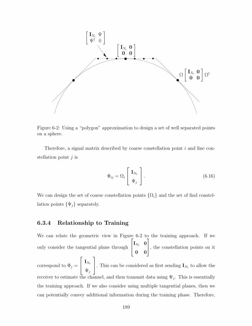
[INt
Ψ
Ψ†0
]
[INt
00 0
]
Ω
[INt
00 0
]Ω†
Figure 6-2: Using a “polygon” approximation to design a set of well separated pointson a sphere.
Therefore, a signal matrix described by coarse constellation point i and fine con-
stellation point j is
Φij = Ωi
INt
Ψj
. (6.16)
We can design the set of coarse constellation points Ωi and the set of find constel-
lation points Ψj separately.
6.3.4 Relationship to Training
We can relate the geometric view in Figure 6-2 to the training approach. If we
only consider the tangential plane through
INt
0
0 0
, the constellation points on it
correspond to Φj =
INt
Ψj
. This can be considered as first sending INt
to allow the
receiver to estimate the channel, and then transmit data using Ψj. This is essentially
the training approach. If we also consider using multiple tangential planes, then we
can potentially convey additional information during the training phase. Therefore,
189
this geometric coding design can be considered as a modified training approach where
the pilot signal can be one of many. This scheme is more complex, but has the
potential to increase data rate.
This additional amount of information turns out to be negligible, at least in the
high SNR limit. As SNR increases, the fine constellation points can become denser
and denser to take advantage of the smaller noise. However, no new tangential planes
can be added. Therefore, the amount of information that can be carried during the
training phase does not grow with SNR, and becomes negligible in the high SNR
limit. In fact, Zheng and Tse showed that training is optimal in terms of diversity-
multiplexing tradeoff [42]. This is because multiplexing gain only focuses on growth
rate; a constant number of bits does not matter.
In summary, this geometric approach translates the non-coherent signal design
problem to one of packing points on a sphere. Further approximation of the sphere
using a set of tangential planes leads to a scheme which is a modified training ap-
proach where the pilot signal itself can carry some fixed amount of information. This
geometric view together with Zheng and Tse’s result suggests that training is a rea-
sonably good approach.
6.4 Channel Training Approach
In this section, we focus on a training approach for non-coherent communication.
In the training scheme we consider, the transmitter first transmit a training signal√SNRINt
for a period of Nt, and then spend the rest of coherence time T − Nt
transmitting data as if the channel is perfectly known at the receiver. This is a very
simplistic scheme. More optimally, the transmitter should consider the fact that the
receiver only has an estimate of the channel after the training phase. But this is more
difficult.
One issue we would like to discuss briefly here relates to the time varying nature
of the channel and the block fading approximation. If the channel were truly block
fading, then the channel we experience during the training and data-transmission
190
phases would be truly identical. We would be able to first spend some time to obtain
a sufficiently good channel estimate and then use it for the rest of the block. However,
in reality, the channel varies in time. Even if we had obtained a very good estimate
of the channel during the training phase, the true channel would have drifted by the
data-transmission phase. As time goes on, the deviation would increase until the
next training phase. Medard, Abou-Faycal, and Madhow [25] studied the possibility
of transmitting at higher rates during times closer to the pilot signal when the channel
estimation error is less and transmitting at lower rates in between when the error is
greater.
In this section, let us still assume the block fading model and focus on the simple
scheme of training plus coherent communication. We first discuss how the receiver can
estimate the channel and what the quality is, and then look at how the performance
is affected by imperfect channel knowledge.
6.4.1 Quality of Channel Estimation
During the training phase, the transmit signal matrix X is the pilot signal X =√SNRINt
. 3 The scaling factor√SNR is chosen such that the power used during
the training phase is the same as the average power used during data-transmission.
It is a reasonable thing to do. It also turns out to be very convenient. If the SNR
available increases and we want to transmit at a higher rate, we will need to have
higher quality channel estimation, and using more energy during training gives us
that.
When X =√SNRINt
, we have
Y = HX+W =√SNRH+W, (6.17)
3Other signals may be used, for example, one with reduced peak power. However, there is nosignificant difference in this context.
191
Written in a component-wise form,
yij =√SNRhij + wij. (6.18)
We can perform scalar minimum mean square error (MMSE) estimation to estimate
hij. The reason for choosing the MMSE estimator is so that the resulting estimation
error is independent from the estimate, and its variance is minimized.
Using standard MMSE formulation, the resulting estimate is
hij =
√SNR
SNR + 1yij. (6.19)
Let us denote the estimation error with ∆H = H − H and δh,ij = hij − hij. It is
easy to show that all δh,ij are IID, circularly symmetric, complex Gaussian random
variables with density CN(0, 2σ2h), where
2σ2h =1
SNR + 1. (6.20)
Note that, as the SNR available to us increases, the variance decreases, and the
channel estimation quality improves. Next, let us look at how the quality of the
channel estimation affects the system performance.
6.4.2 Effect of Imperfect Channel Knowledge
After training, we obtain an estimate of the true channel coefficients. Conditioned
on the received signal yij, each channel coefficient hij is complex Gaussian with den-
sity CN
( √SNR
SNR+1yij,
1SNR+1
). Therefore, we effectively have a Rician channel . The
receiver knows both the mean and the variance of the channel coefficients, while the
transmitter only knows the variance but not the mean. This is different from the
coherent case, where H is deterministic at the receiver and is also different from the
non-coherent case, where H has (zero mean) Rayleigh density.
Ideally, during the data-transmission phase, the transmitter and receiver should
employ a scheme specific for the Rician channel. However, this is beyond the scope of
192
our study. Instead, we simply use the coherent communication schemes studied earlier
and treat the channel estimation error as a form of noise. We discuss its performance
and argue that there is effectively no loss in terms of diversity and multiplexing gains.
We can re-write the channel during the data-transmission phase as
Y = HX+W = HX+∆HX+W. (6.21)
In the first term, H is perfectly known to the receiver. This is similar to coherent
detection. The second term ∆HX can be treated as a new additive noise. Entries of
∆H have variance 1SNR+1
≈ 1SNR
and X has energy on the order of SNR. Consequently,
∆HX has energy on the order of 1, which is also the noise variance. This means
that the new noise ∆HX and the original AWGNW have energy on the same order.
Therefore, by doing simple coherent communication treating H as the trueH, we only
increase the amount of noise by a constant factor. Effectively, this cost only appears
as a constant dB loss in SNR, which means that the diversity and multiplexing gains
achieved are not affected.
The question of how good channel estimation needs to be was also studied by
Lapidoth and Shamai in [18]. They suggested that the channel estimation error
should be small compared to 1SNR
to avoid significant performance degradation.
It is worth noting that the new noise ∆HX is not quite the same as the original
AWGN W. First of all, for a given X, the variance of ∆HX is a function of X.
Although the variance is on the order of 1, it does fluctuate with X. Also, averaging
over X, the distribution of ∆HX is not really Gaussian. It is the average of many
zero mean Gaussian distributions. This being said, it is plausible that treating it as
Gaussian probably does not influence the performance much.
There is another important difference between the noise terms. After the initial
training, ∆H is fixed within one block. If it happens to be large, then we are stuck
with a large noise for an entire block of T , even though ∆HX has energy of order 1
on average. On the other hand, all entries of W are independent. The consequence
of this difference is that, while we can use coding to average large and small entries of
193
W within one block, we are not able to do that for ∆H. However, since short codes
can achieve the same tradeoff as long ones, we expect the inability to do coding to
not affect the diversity-multiplexing tradeoff.
Earlier when we argued for ∆HX and W having energy on the same order, we
needed the variance of ∆H to be on the order of 1SNR
. This is true if we have true
block fading and the training signal has energy on the order of SNR. If the channel
were slowly varying, then a certain time after the training phase, the channel would
have drifted by a certain amount independent of SNR. This would contribute to a
component of the estimation error that is not order 1SNR
. When this happens, ∆HX
would be much greater than W as SNR grows. Therefore, at high SNR, we might
have to train more frequently before ∆H becomes too large.
194

Chapter 7
Summary and Future Directions
7.1 Contributions
In this thesis, we studied the problems of efficient designs for multiple antenna com-
munication systems. We studied the design problems in various delay and complexity
regimes, from uncoded systems, to structured codes with short delay, to long error
correction code enhanced systems.
The main advantages of multiple antennas communication over traditional single
antenna communication are the rate gain and robustness gain toward channel fading.
To better achieve these gains, we focused on the perspective of diversity-multiplexing
tradeoff, a framework established by Zheng and Tse [41], which describes how fast rate
increases and how rapidly error probability decays with SNR. We used this diversity-
multiplexing tradeoff as a measure of goodness to evaluate systems through out the
thesis. As systems become more complex and the code length becomes longer, better
tradeoff can be achieved.
In chapter 2, we reviewed the diversity-multiplexing tradeoff framework and also
provided some of our own intuitions. We measured the the horizontal spacings be-
tween a family of error probability curves and the slopes of these curves to evaluate
the diversity-multiplexing tradeoff. This family of curves not only captures the re-
lationship between rate, SNR, and error probability, in the finite SNR regime, but
also allows us to see the limiting tradeoff behaviors. We evaluated systems by plot-
195
ting families of error probability curves and comparing them to the family of outage
probability curves.
In section 2.3.5, we briefly discussed the concept of local diversity-multiplexing
tradeoff. In certain situations, system designers may care about how the performance
of an existing system changes when the operating parameters change slightly, such as
when more SNR becomes available, or when the desired data rate increases. In these
cases, the local tradeoff is the quantity of interest.
We also discussed the relationship between different segments of the diversity-
multiplexing tradeoff curve and the different regions of the (SNR, Pe, R) parameter
space. Depending on where the system designer wants to operate in, different seg-
ments of the tradeoff curve should be focused on. In particular, for higher rates, the
segment of the tradeoff corresponds to larger r is important.
For most of this thesis, we focused on two-transmit two-receive antenna systems,
which arises frequently in practice. Even though it is small, this system can provide
significant gains over single antenna systems.
In chapter 3, we introduced a lattice-reduction-aided detection idea. By operating
traditional low-complexity detectors in a lattice reduced basis, we can achieve near
optimal performance with low complexity. In particular, we can achieve the same
diversity as the more-complex maximum likelihood detectors, and can achieve the
optimal diversity-multiplexing tradeoff achievable by any length-one code. This idea
is mainly for low dimensional cases. When extended to higher dimensions, it quickly
becomes complex. It can also be used at the transmitter as a pre-coding technique.
One main problem with this detector is that it does not treat the boundary of the
constellation. Because of this problem, it can not be combined with the tilted-QAM
code introduced in chapter 4 to achieve the same tradeoff that ML detectors can.
In chapter 4, we proposed a tilted-QAM code design for the two-transmit two-
receive antenna channel that can achieve the optimal diversity-multiplexing tradeoff
curve with code length two. This answers the previously open question of whether the
optimal tradeoff is achievable at this length. This code improves upon the OSTBC
by replacing the repetition used with a rotation, thus avoiding the multiplexing gain
196
loss. At high SNR, tilted-QAM code is increasing better than OSTBC; however, at
low SNR, OSTBC is preferred for its low complexity.
In the tilted-QAM code, one key feature is a set of universally optimal rotation
angles that leads to the same worst case determinant for all rates. Similar rotation
ideas have been previously studied, but the existence of the universally optimal rota-
tion angles was unknown. This result can also be applied elsewhere, for example, to
single antenna communication over multiple fades, as discussed in section 4.6.
We evaluated the performance of the tilted-QAM code from two different per-
spectives. These error evaluation techniques developed may potentially be used to
evaluate other deterministic codes and be extended to higher dimensional cases.
In chapter 5, we investigated using powerful error correction codes in multiple
antenna systems to build practical systems with good performance. We explored
many schemes and a wide range of possibilities. For low SNR regime, we showed that
the low-complexity OSTBC scheme is near optimal. However, for higher SNR levels
and systems with more antennas, further research is needed. D-BLAST system is
shown to be theoretically optimal but suffers from problems such as error propagation.
Other block form variations of BLAST require joint decoder to do well. We also tested
system that combine tilted-QAM code with error correction codes. The Hard-decision
based system can reach 5 dB from capacity with moderate complexity; while the soft-
decision one reduces the gap to 3 dB, but increases the decoding complexity.
In chapter 6, we studied the case of non-coherent communication where neither
the transmitter nor the receiver knows the channel. We reviewed several coding
designs and a graphical view that relates coding for non-coherent communication to
packing on a sphere. By approximating the sphere with tangential planes, we turned
the signal design problem into a problem of designing a set of coarse points plus
doing coherent communication coding within the planes. We concluded that training
scheme corresponds to using just one of the planes and the loss in rate is a constant
factor.
197

7.2 Future Directions
7.2.1 Coherent Communications
One interesting future direction of research is to extend the tilted-QAM code design
to higher dimensions. This is a challenging problem due to the higher number of
dimensions and the larger number of variables. One open question we hope to an-
swer is the achievability of optimal diversity multiplexing tradeoff using codes with
length Nt ≤ T < Nt + Nr − 1. Gaussian random codes at these lengths are sub-
optimal. However, it might be possible to construct deterministic codes that can
reach optimality.
Another theoretically interesting topic is the design criteria in higher dimensional
cases. In the two-transmit two-receive antenna case, we saw that maximizing the
worst-case determinant is important for achieving the optimal tradeoff for 0 ≤ r ≤ 1,
while keeping the degree of freedom and not use repetition is important for achieving
the maximum multiplexing gain. In higher dimensional cases, the optimal tradeoff
curve has more linear segments, we suspect that there are different criteria for the
different segments, and these criteria need to be identified. Also, since the different
segments correspond to different (SNR, Pe, R) regimes, depending on the operating
point, we might need to focus on different criteria.
More practically, if more antennas are available, we can consider using the 2 × 2
tilted-QAM code as a building block. For example, in a Nt = Nr = T = 4 system, if
we encode for the four antennas using two independent 2× 2 tilted-QAM codes and
do ML decoding, we expect that a maximum diversity of 8 can be achieved, instead
of NtNr = 16. This loss is acceptable practically, since the target error rate needed
are usually not too low. More work involving how 2×2 tilted-QAM code can be used
as a component in systems with more antennas may lead to practical schemes.
Another practical problem that needs to be solved is the joint decoding problem
for V-BLAST or X-BLAST. We saw that X-BLAST can achieve optimal performance
if joint decoding can be done. Therefore, if joint decoding can be done efficiently, this
may lead to many practical applications.
198
In order to do joint decoding, we must deal with the interference between the
transmitted symbols. One low-complexity way to do so is to use the lattice-reduction-
aided detectors. We saw earlier that this does not work due to the boundary problem
of lattice decoding. Therefore, if we could deal with the boundary efficiently, it might
lead to a way of doing joint decoding efficiently and well enough such that the optimal
tradeoff can be achieved.
7.2.2 Non-coherent Communications
The field of non-coherent communication is still a wide open one. Developing deeper
understanding of this problem is very important, because the channel is never known
perfectly at the receiver in reality. When systems developed with the channel knowl-
edge assumption are implemented in practice, engineers often have to deal with chan-
nel uncertainty issues. If systems could be designed from non-coherent communication
theory, they might lead to more robust implementations in practice.
The geometric approach presented in section 6.3 allows existing coherent multiple
antenna communication techniques to be applied to the non-coherent case. This may
be a promising approach. Directly solving the non-coherent problems seems difficult.
Leveraging on existing coherent communication techniques may make the problem
easier. One of the key problems that still need to be resolved along this path is how
large the tangential planes can be before the approximation of the sphere becomes
bad near the edge. This effect also appears in the case of coherent communication
with training, in that channel estimation error causes more interference for points
at the edge of the constellation. Another key problem is the design of the coarse
constellation points. From the size limit of the tangential planes, we can estimate
how many coarse constellation points are needed. If this number is small, we may
be able to use existing techniques or use very special structures. However, if a large
number of points is needed, the design may be difficult.
Among the existing non-coherent communication results, most are developed us-
ing the block fading model. This assumption that the channel stays exactly constant
could be mis-leading. It allows for techniques such as learning the channel as accu-
199
rately as desired at the beginning and then treat the channel as coherent, which is not
possible if the channel is fading continuously. One consequence of this discrepancy is
that the capacity growth rate at high SNR is different depending on the model used.
Another problem associated with the block fading model is the choice of the
coherence time T , the period in which we assume the channel stays exactly constant.
If T were set to be too large, the channel could change significantly within one block,
invalidating the block fading assumption. If T were set to be too small, the channel
seen by neighboring blocks would be quite close, and not taking advantage of this
correlation is inefficient.
One non-coherent signal design that does not used the block fading model and
avoids the above problem is the differential coding scheme. It uses small blocks
and assumes the channel does not change much between neighboring blocks. Slight
channel variations are treated as noise. This scheme may be further improved by
considering the channel variation across blocks.
Generally, further research based on more accurate continuous fading models is
needed to understand its effect and how good block fading model really is.
In terms of theoretical results, one that is useful but may be difficult to develop
is the capacity achievable at low SNR. This result is important for evaluating system
performance in practical regimes.
200

Bibliography
[1] S. M. Alamouti. A simple transmit diversity technique for wireless communi-
cations. IEEE Journal on Selected Areas in Communications, 16(8):1451–1458,
October 1998.
[2] A. H. Banihashemi and A. K. Khandani. On the complexity of decoding lattices
using the korkin-zolotarev reduced basis. IEEE Transactions on Information
Theory, 44(1):162–171, January 1998.
[3] J. Boutros and E. Viterbo. Signal space diversity: a power- and bandwidth-
efficient diversity technique for the rayleigh fading channel. IEEE Transactions
on Information Theory, 44(4):1453–1467, July 1998.
[4] G. Caire, G. Taricco, and E. Biglieri. Bit-interleaved coded modulation. IEEE
Transactions on Information Theory, 36:726–740, July 1990.
[5] J. H. Conway, R. H. Hardin, and N. J. A. Sloane. Packing lines, planes, etc.,
packings in grassmannian spaces. Experimental Mathematics, 5:139–159, 1996.
Download available at http://www.research.att.com/ njas/grass/index.html.
[6] J. H. Conway and N. J. A. Sloane. Sphere packing, lattices and groups. Springer-
Verlag, New York, 2 edition, 1993.
[7] T. M. Cover and J. A. Thomas. Elements of information theory, Wiley Series
in Telecommunications. Wiley, New York, 1991.
201

[8] M. O. Damen, A. Tewfik, and J-C. Belfiore. A construction of a space-time code
based on number theory. IEEE Transactions on Information Theory, 48(3):753–
760, March 2002.
[9] G. J. Foschini. Layered space-time architecture for wireless communication in a
fading environment when using multiple antennas. Bell Laboratories Technical
Journal, 1(2):41–59, Autumn 1996.
[10] R. G. Gallager. Low-density parity check codes. MIT Press, Cambridge, MA,
1963.
[11] B. Hochwald and W. Sweldens. Differential unitary space time modulation. IEEE
Transactions on Communications, 48(12):2041–2052, December 2000.
[12] B. M. Hochwald and T. L. Marzetta. Unitary space-time modulation for multiple-
antenna communications in rayleigh flat fading. IEEE Transactions on Informa-
tion Theory, 46(2):543–564, March 2000.
[13] B. M. Hochwald, T. L. Marzetta, and T. J. Richardson. Systematic design of
unitary space-time constellations. IEEE Transactions on Information Theory,
46(6):1962–1973, September 2000.
[14] B. M. Hochwald and S. ten Brink. Achieving near-capacity on a multiple-antenna
channel. IEEE Transactions on Communications, 51(3):389–399, March 2003.
[15] A. Korkin and B. Zolotarev. Sur les formes quadratiques. Math. Ann., 6:366–389,
1873.
[16] A. Lapidoth and S.M. Moser. Convex-programming bounds on the capacity
of flat-fading channels. Proc. IEEE International Symposium on Information
Theory, page 52, 2001.
[17] A. Lapidoth and S.M. Moser. On the fading number of multi-antenna systems.
Proc. IEEE Information Theory Workshop, pages 110–111, 2001.
202
[18] A. Lapidoth and S. Shamai. Fading channels: how perfect need ”perfect side
information” be? IEEE Transactions on Information Theory, 48(5):1118–1134,
May 2002.
[19] E. A. Lee and D. G. Messerschmitt. Digital Communication. Kluwer Academic
Publishers, Norwell, MA, 2 edition, 1993.
[20] A. K. Lenstra, H. W. Lenstra, and L. Lovasz. Factoring polynomials with rational
coefficients. Math. Annalen, 261:513–534, 1982.
[21] H. W. Lenstra. Integer programming with a fixed number of variables. Math. of
Operations Res., 8:538–548, November 1983.
[22] L. Lovasz. An algorithmic theory of numbers, graphs, and convexity. NSF-CBMS
Regional Conference Series in Applied Mathematices 50 : Society for Industrial
and Applied Mathematics, 1986.
[23] T. L. Marzetta, B. Hassibi, and B. M. Hochwald. Structured unitary space-time
autocoding constellations. IEEE Transactions on Information Theory, 48(4):942
–950, April 2002.
[24] T. L. Marzetta and B. M. Hochwald. Capacity of a mobile multiple-antenna
communication link in rayleigh flat fading. IEEE Transactions on Information
Theory, 45(1):139–157, September 1999.
[25] M. Medard, I. Abou-Faycal, and U. Madhow. Adaptive coding with pilot signals.
38th Annual Allerton Conference on Communication, Control, and Computing,
October 2000.
[26] M. Pohst. On the computation of lattice vectors of minimal length, successive
minima and reduced basis with application. ACM SIGSAM Bull., 15:37–44,
1981.
[27] A. S. Y. Poon, D. N. C. Tse, and R. W. Brodersen. Multiple-antenna channels
from a combined physical and networking perspective. Asilomar Conference for
Signals, Systems, and Computers, November 2002.
203
[28] N. Prasad and M. Varanasi. Optimum efficiently decodable layered space-time
block code. Proc. Asilmar Conf. Signals, Systems, and Computers, November
2001.
[29] J. G. Proakis. Digital communications. McGraw-Hill, New York, NY, 4 edition,
2001.
[30] B. Rimoldi and R. Urbanke. A rate-splitting approach to the gaussian multiple-
access channel. IEEE Transactions on Information Theory, 42(2):364–375,
March 1996.
[31] S. Sandhu and A. Paulraj. Unified design of linear space-time block codes. IEEE
Global Telecommunications Conference, 2:1073–1077, 2001.
[32] C. P. Schnorr. A hierarchy of polynomial time lattice basis reduction algorithms.
Theory of Computer Science, 53:201–224, 1987.
[33] V. Tarokh and H. Jafarkhani. A differential detection scheme for transmit di-
versity. IEEE Journal on Selected Areas in Communications, 18(7):1169–1174,
July 2000.
[34] V. Tarokh, H. Jafarkhani, and A. R. Calderbank. Space-time block codes from
orthogonal designs. IEEE Transactions on Information Theory, 45(5):1456–1467,
July 1999.
[35] V. Tarokh, N. Seshadri, and A. R. Calderbank. Space-time codes for high data
rate wireless communication: performance criterion and code construction. IEEE
Transactions on Information Theory, 44(2):744–765, March 1998.
[36] E. Telatar. Capacity of multi-antenna gaussian channels. AT&T Bell Labs In-
ternal Tech. Memo., June 1995.
[37] E. Visotsky. Space-time transmit precoding and interference suppression for a
wireless downlink. PhD thesis, University of Illinois at Urbana-Champaign, 2000.
204
[38] E. Viterbo and J. Boutros. A universal lattice code decoder for fading channels.
IEEE Transactions on Information Theory, 45(5):1639–1642, July 1999.
[39] P. W. Wolniansky, G. J. Foschini, G. D. Golden, and R. A. Valenzuela. V-blast:
an architecture for realizing very high data rates over the rich-scattering wireless
channel. URSI International Symposium on Signals, Systems, and Electronics
(ISSSE), pages 295–300, September 1998.
[40] L. Zheng and D. N.C. Tse. Communicating on the grassmann manifold: a
geometric approach to the non-coherent multiple antenna channel. IEEE Trans-
actions on Information Theory, 48(2):359–383, February 2002.
[41] L. Zheng and D. N.C. Tse. Diversity and multiplexing: a fundamental tradeoff
in multiple antenna channels. to appear in IEEE Transactions on Information
Theory, 2002.
[42] L. Zheng and D. N.C. Tse. The diversity-multiplexing tradeoff for non-coherent
multiple antenna channels. Proc. of Allerton Conference on Communication,
Control, and Computing, October 2002.
205
Related Documents


