© Xia Chun 30 30 30 30 Efficient Frontier Implementation Problems (1) Many portfolios on the MVE Frontier require shorting securities, and often massive amounts so. Same applies to the short-constrained MVE frontier, which usually lies entirely inside the unconstrained MVE frontier. Learn how to construct efficient frontier using spreadsheet Download an example file from WebCT Recall shorting is mainly used by hedge fund, but not others. 30 Source: Chapter 7 Appendix A, textbook 231-236

Welcome message from author
This document is posted to help you gain knowledge. Please leave a comment to let me know what you think about it! Share it to your friends and learn new things together.
Transcript
© Xia Chun 30303030
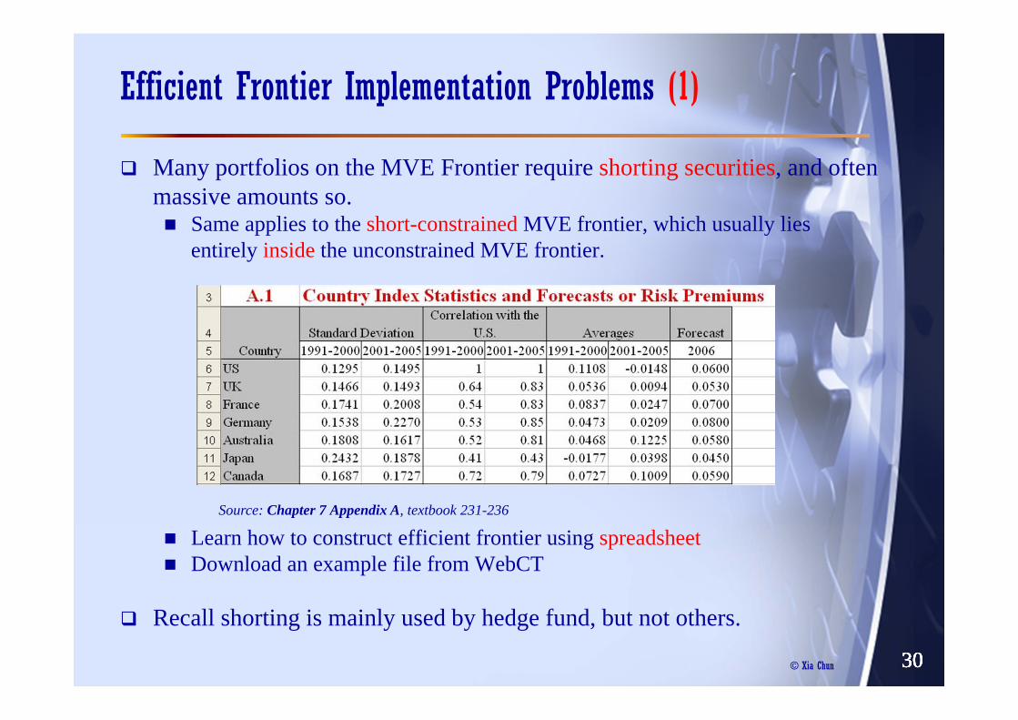
Efficient Frontier Implementation Problems (1)
Many portfolios on the MVE Frontier require shorting securities, and often massive amounts so.
Same applies to the short-constrained MVE frontier, which usually lies entirely inside the unconstrained MVE frontier.
Learn how to construct efficient frontier using spreadsheetDownload an example file from WebCT
Recall shorting is mainly used by hedge fund, but not others.
30
Source: Chapter 7 Appendix A, textbook 231-236

© Xia Chun 31313131
The Optimal Weights and The Big Troubles
Figure 7A.2: Efficient Frontier and CAL for Seven Country Stock Indexes
0.03
0.04
0.05
0.06
0.07
0.08
0.09
0.10 0.12 0.14 0.16 0.18 0.20 0.22 0.24
Efficient FrontierCapital Allocation LineEff Front - No Short
Too large short positions Impose a constraint, with new trouble

© Xia Chun 32323232
Efficient Frontier Implementation Problems (2)
No one really knows how to estimate future expected rates of return well.You must use your own judgment when the result is reasonable.
Industry hires macro/IO guys as strategists/analysts
Risk is a different concept for different person and organization. Measured using different method, different time horizonThat is why funds are so diverseTheoretically there is a globally efficient frontier. But it is unrealistic to construct it, too costly.
The optimization technique requires very large number of estimate inputs. and is very sensitive to any estimation errors.
e.g., to find tangency portfolio from 3000 stocks, need 4,504,500 estimate, including expected return, variance and covariance. a big trouble before 1970sIndustry came up “factor model” to address this trouble (our next lecture)
32

© Xia Chun 373737
What’s the main drawback of Markowitz technique?Concentrated position; Sensitive to estimate error; Subjective view not allowed
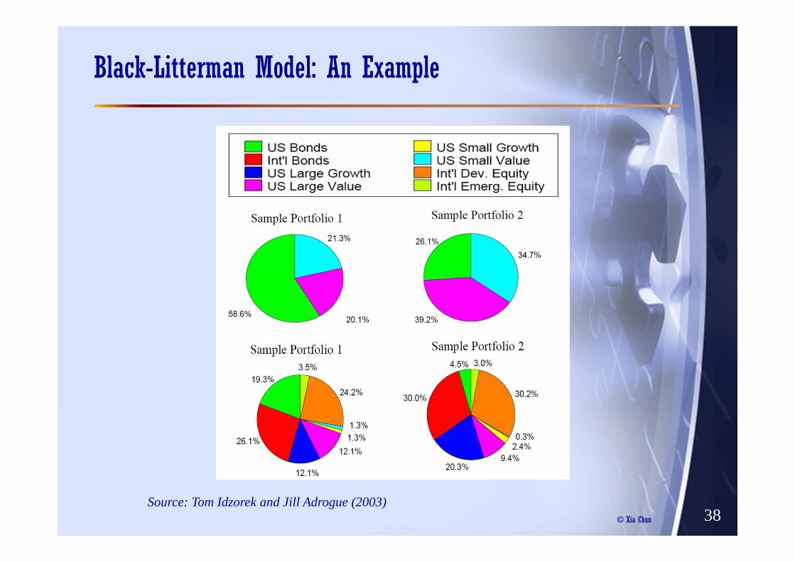
The Black-Litterman Bayesian asset allocation model is one of the most sophisticated and widely used tools in asset management. It was developed in Goldman Sachs in early 1990s.
BL assumes that the initial expected returns should be equal to what is implied by market equilibrium choices (CAPM or APT). The user is only required to state how her views about expected returns differ from the market's and to state her degree of confidence in the alternative views.
estimate the covariance matrix from historical data (more stable)determine a baseline (prior) forecastintegrate the manager’s private views and confidencedevelop revised (posterior) forecast and apply portfolio optimization
Chapter 27 gives the formula. You can also refer to recommended books.
CASE Black-Litterman Model
© Xia Chun
Black-Litterman Model: An Example
38Source: Tom Idzorek and Jill Adrogue (2003)

© Xia Chun
A Three-Stock Example
Suppose Pc = 1. Consider a portfolio with weights on A, B, C, (-1, 1, 1)The portfolio use zero capital.The payoff in each state:
Suppose Pc = 4. Consider weights (2, -1, -1)The portfolio use zero capital.The payoff in each state:
4
Stock A B CFuture State 1 10 8 9Future State 2 8 0 12Current Price 3 2 ?
state 1: 10 ( 1) 8 1 9 1 7 0state 2: 8 ( 1) 0 1 12 1 4 0
× − + × + × = >× − + × + × = >
state 1: 10 2 8 ( 1) 9 ( 1) 3 0state 2: 8 2 0 ( 1) 12 ( 1) 4 0
× + × − + × − = >× + × − + × − = >

© Xia Chun
Do You Have The Crystal Ball?
We can show Pc = 3 by solving the following equations:
In practice, it is hard to forecast future payoffs in different states.We can rely on factor model which summarizes past information
Risk-free arbitrage is rare. Arbitrage activities must be risky!
5
Stock A B CFuture State 1 10 8 9Future State 2 8 0 12Current Price 3 2 ?
1 2 3
1 2 3
1 2 3
initial outlay: 3 2 0state 1 payoff: 10 8 9 0state 2 payoff: 8 0 12 0
cw w p ww w w
w w w
+ + =× + × + × =
× + × + × =

© Xia Chun 66666
APT Assumptions
Stephen Ross developed no-arbitrage pricing theory in 1976.
1. Security returns can be described by a factor model.Theory is silent about factors.
2. There are sufficient securities to diversify away idiosyncratic/firm-specific risk.
3. Well-functioning security markets do not allow for the persistence of arbitrage opportunities, or the presence of arbitrageur corrects mispricing.
CAPM has three major assumptions. The difference is quite obvious.
1. Mean-variance preferences
2. Perfect frictionless capital market
3. Identical information and homogeneous expectations

© Xia Chun 33333
Empirical Testing of CAPM
Why should we care?Theoretical consideration: test if the theory is validPractical consideration: use theory to determine cost of capital, to discover money-making opportunity, to design investment strategies, etc
The basic prediction of the CAPM is that market portfolio is mean-variance efficient (no matter whether risk-free rate exists or not). This requirement can provide a direct test of CAPM.
Complication: market portfolio will almost always be ex-post mean-variance-inefficient, even if it is ex-ante efficient.Hence cannot be tested directly
The security market line (SML) is then a further set of predictions based on the efficiency of the market portfolio. This constitutes a secondary form of test.
Two versions of CAPM: the Sharpe-Lintner form and the Black form
3

© Xia Chun 44444
Sharpe-Lintner Form
Sharpe-Lintner recognize the empirical proxy for risk-free rate could be stochastic
The CAPM implies relationships between expected (ex ante) returns, whereas we can observe are actual or realized (ex post) returns,
The empirical counterpart is the security characteristic line (SCL) :
Residual terms are assumed uncorrected across time and assetsActually they are correlated!Test would be more precise if it is run on beta-grouped portfolios rather than on individual stocks as residual terms diversified away.
Two-pass regression, first get beta from SCL estimation, then test SML.See textbook p.411-415.
( , )( ) ( ) where ( )
i Mi i M i i f i
M
Cov R RE R E R R r rVar R
β β= = − =
it i i Mt itR Rα β ε= + +
4

© Xia Chun 555
Two-Pass Regression and Hypotheses
Time-series regression (SCL estimation)
Assume 100 assets and a market index and risk-free asset, and 10 years annual data
100 regressions, 100 SCL’s
Cross-sectional regression (SML estimation)
1 regression, 1 SML
1 1 1 1
2 2 2 2
10 10 10 10
0
ˆˆ
Do this for each asset ˆH : 0
i f M f
i f M fi i
i f M f
i
r r r rr r r r
r r r r
α β
α
− −⎛ ⎞ ⎛ ⎞⎜ ⎟ ⎜ ⎟− −⎜ ⎟ ⎜ ⎟= +⎜ ⎟ ⎜ ⎟⎜ ⎟ ⎜ ⎟⎜ ⎟ ⎜ ⎟− −⎝ ⎠ ⎝ ⎠
=
M M
1 1
2 20 1 2
100 5
0 0
0 2
0 1
ˆ
ˆˆ ˆ ˆ
ˆ
ˆH : 0ˆ ˆH : capture all variation, 0
ˆH :
t ft
t ft
t ft
Mt ft
r r
r rChar
r r
r r
β
βγ γ γ
β
γ
β γ
γ
⎛ ⎞ ⎛ ⎞−⎜ ⎟ ⎜ ⎟
−⎜ ⎟ ⎜ ⎟= + +⎜ ⎟ ⎜ ⎟
⎜ ⎟ ⎜ ⎟⎜ ⎟⎜ ⎟− ⎝ ⎠⎝ ⎠
=
=
= −
M M
say, size, β2, residual variance σ2(ei), etc
Note: if regress realized return rather than excess return, some hypotheses change
© Xia Chun 66666
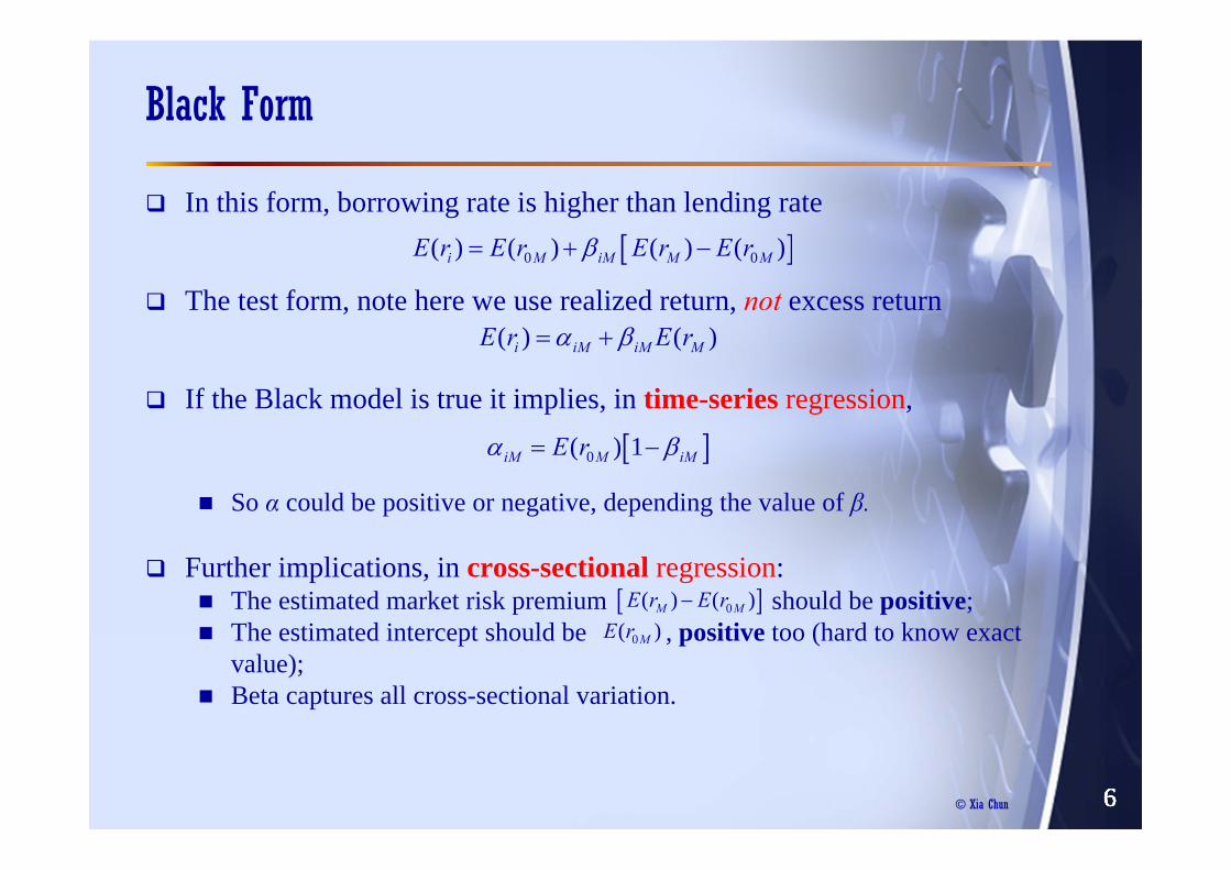
Black Form
In this form, borrowing rate is higher than lending rate
The test form, note here we use realized return, not excess return
If the Black model is true it implies, in time-series regression,
So α could be positive or negative, depending the value of β.
Further implications, in cross-sectional regression:The estimated market risk premium should be positive;The estimated intercept should be , positive too (hard to know exact value); Beta captures all cross-sectional variation.
[ ]0 0( ) ( ) ( ) ( )i M iM M ME r E r E r E rβ= + −
( ) ( )i iM iM ME r E rα β= +
[ ]0( ) 1iM M iME rα β= −
6
[ ]0( ) ( )M ME r E r−
0( )ME r

© Xia Chun 1313131313
Black, Jensen, and Scholes (1972): Portfolio Construction
Note that in Jensen (1968) the residuals are correlated which invalidates the simple test.
overcome by using portfolios, but this reduce sample size in second-pass.choose to group assets to obtain maximum dispersion in betas of the portfoliosRandomly formed, betas for most portfolio are close to one (recall lecture 7).
Data from 1926- 1965 (data up to Mar 1966)First rank stocks on basis of betas estimated on the basis of the 5 years of data from 1926 to 1930 (using equally-weighted NYSE stocks as the market portfolioConstruct 10 portfolios with highest beta stock in portfolio 1, and so on downwards until portfolio 10. Compute return on each portfolio for the 12 months of 1931. Next repeat the step for stock from 1927 to 1931. Reform 10 portfolios. Compute their monthly returns in 1932Repeat this process through to 1965. (then calculate return up to Mar 1966 )
For each portfolio, [12 (month) × 35 (year)=420] number of returns 13

© Xia Chun
Portfolio Sort on Beta
14

© Xia Chun 1515151515
Black, Jensen, and Scholes (1972): Two-Pass Regression
Then estimate the alphas and betas of the 10 portfolios by using 35 years of monthly return data (the time series analysis).
Findings: the alphas for the high beta portfolios tend to be negative, and positive for the low beta portfolios.
Bad news to Sharpe-Lintner CAPMOK for Black as
Then the cross-section analysis.
Finding: a market risk premium of 12.972% per year (on estimated SML, 1.081% per month), less than average excess market return 17.04%
The intercept is annual of 6.228% (on estimated SML, 0.519% per month), higher than the average interest rate on risk-free bonds.
More consistent with Black CAPMBoth estimates are positive.
15
[ ]0( ) 1iM M iME rα β= −

© Xia Chun 1616161616
Summary of Early Empirical Testing
Firmly reject the Sharpe-Lintner CAPM. There is a positive relation between beta and average return, but it is “flat”.
Same for recent data.If Sharpe-Linter CAPM is good, then the expected market excess return should be equal to realized mean excess return (17.04%).
More consistent with the Black CAPM. But this less restrictive model eventually succumb to the data after 1980.
The slope becomes zero and beta does not explain return variation!
16
Beta
AnnualReturn
Theoretical SML
Fitted/Estimated SML
6.228% Slope=12.972%
Slope=17.04%
© Xia Chun
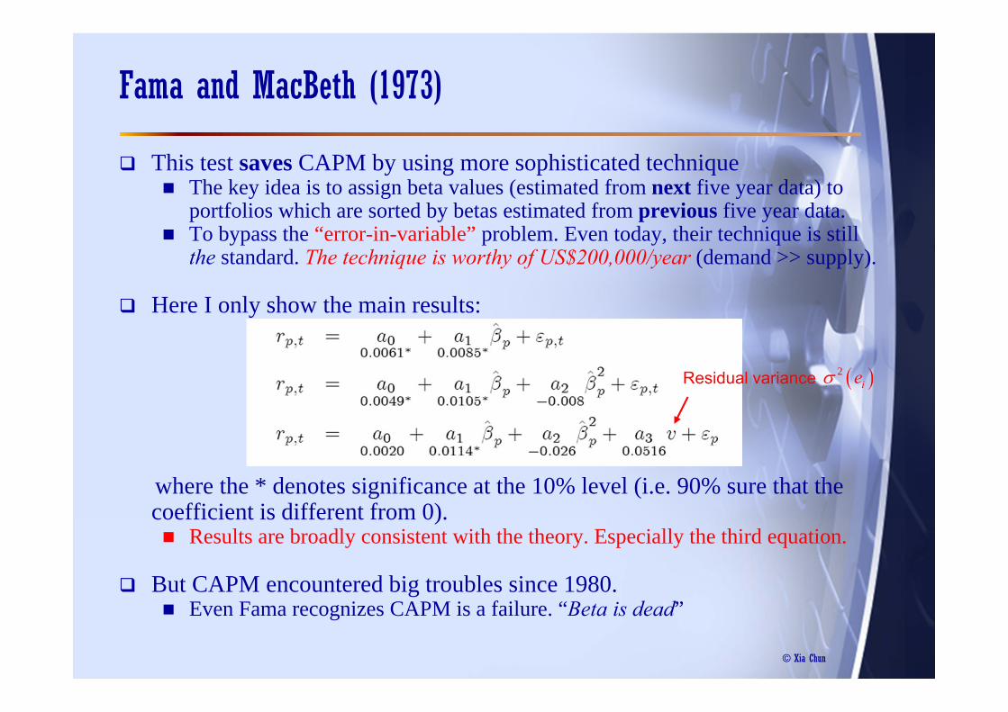
Fama and MacBeth (1973)
This test saves CAPM by using more sophisticated techniqueThe key idea is to assign beta values (estimated from next five year data) to portfolios which are sorted by betas estimated from previous five year data.To bypass the “error-in-variable” problem. Even today, their technique is still the standard. The technique is worthy of US$200,000/year (demand >> supply).
Here I only show the main results:
where the * denotes significance at the 10% level (i.e. 90% sure that the coefficient is different from 0).
Results are broadly consistent with the theory. Especially the third equation.
But CAPM encountered big troubles since 1980. Even Fama recognizes CAPM is a failure. “Beta is dead”
Residual variance ( )2ieσ
Related Documents