Efficient estimation of a semiparametric partially linear varying coefficient model

arX

iv:m

ath/

0504

510v

1 [

mat

h.ST

] 2

5 A

pr 2

005

The Annals of Statistics

2005, Vol. 33, No. 1, 258–283DOI: 10.1214/009053604000000931c© Institute of Mathematical Statistics, 2005

EFFICIENT ESTIMATION OF A SEMIPARAMETRIC PARTIALLY

LINEAR VARYING COEFFICIENT MODEL

By Ibrahim Ahmad, Sittisak Leelahanon and Qi Li1

University of Central Florida, Thammasat University

and Texas A&M University

In this paper we propose a general series method to estimate asemiparametric partially linear varying coefficient model. We estab-lish the consistency and

√n-normality property of the estimator of

the finite-dimensional parameters of the model. We further show that,when the error is conditionally homoskedastic, this estimator is semi-parametrically efficient in the sense that the inverse of the asymptoticvariance of the estimator of the finite-dimensional parameter reachesthe semiparametric efficiency bound of this model. A small-scale sim-ulation is reported to examine the finite sample performance of theproposed estimator, and an empirical application is presented to il-lustrate the usefulness of the proposed method in practice. We alsodiscuss how to obtain an efficient estimation result when the error isconditional heteroskedastic.

1. Introduction. Semiparametric and nonparametric estimation techniqueshave attracted much attention among statisticians and econometricians. Onepopular semiparametric specification is a partially linear model as consid-ered by Robinson (1988), Speckman (1988) and Stock (1989), among others,via

Yi = v′iγ + δ(zi) + ui, i = 1, . . . , n,(1)

where the prime denotes transpose, v′iγ is the parametric component andδ(zi) is an unknown function and, therefore, is the nonparametric componentof the model; see Green and Silverman (1994), Hardle, Liang and Gao (2000)and the references therein for more detailed discussion of this model. This

Received March 2002; revised February 2004.1Supported in part by the Private Enterprise Research Center, Texas A&M University.AMS 200 subject classification. 62G08.Key words and phrases. Series estimation method, partially linear, varying coefficient,

asymptotic normality, semiparametric efficiency.

This is an electronic reprint of the original article published by theInstitute of Mathematical Statistics in The Annals of Statistics,2005, Vol. 33, No. 1, 258–283. This reprint differs from the original in paginationand typographic detail.

1

http://arXiv.org/abs/math/0504510v1

http://www.imstat.org/aos/

http://dx.doi.org/10.1214/009053604000000931

http://www.imstat.org

http://www.imstat.org

http://www.imstat.org/aos/

http://dx.doi.org/10.1214/009053604000000931

2 I. AHMAD, S. LEELAHANON AND Q. LI

model can be generalized to the following semiparametric varying coefficientmodel:

Yi = v′iγ(zi) + δ(zi) + ui, i = 1, . . . , n,(2)

where γ(z) is a vector of unknown smooth functions of z. Define xi = (1, v′i)′

and β(z) = (δ(z), γ(z)′)′. Then (2) can be written more compactly as

Yi = x′iβ(zi) + ui, i = 1, . . . , n.(3)

The varying coefficient model is an appropriate setting, for example, in theframework of a cross-sectional production function where vi = (Labori,Capitali)

′

represents the firm’s labor and capital inputs, and zi = R&Di is the firm’sresearch and development expenditure. The varying coefficient model sug-gests that the labor and capital input coefficients may vary directly with thefirm’s R&D input, so the marginal productivity of labor and capital dependon the firm’s R&D values. While the partially linear model (1) only allowsthe R&D variable to have a neutral effect on the production function, thatis, it only shifts the level of the production frontier, it does not affect thelabor and/or capital marginal productivity. Li, Huang, Li and Fu (2002) usethe nonparametric kernel method to estimate the semiparametric varyingcoefficient model (2) and apply the method to China’s nonmetal mineralmanufacturing industry data; their results show that the semiparametricvarying coefficient model (2) is more appropriate than either a parametriclinear model or a semiparametric partially linear model for studying theproduction efficiency in China’s nonmetal mineral manufacturing industry.

The time-series smooth transition autoregressive (STAR) model is an-other example of the varying coefficient model. It is given by yt = x′

tβ(yt−d)+ut, where β(yt−d) is a vector of bounded functions; see Chen and Tsay (1993)and Hastie and Tibshirani (1993). They consider an autoregressive modelof the form yt = f1(yt−d)yt−1 + f2(yt−d)yt−2 + · · ·+ fp(yt−d)yt−p + ut, wherethe functional forms of the fj(·)’s (j = 1, . . . , p) are not specified. Chen andTsay (1993) and Hastie and Tibshirani (1993) discuss the identification offj(·) and suggest some recursive algorithms to estimate the unknown func-tion fj(·). More recent work on varying coefficient models can be found inCarroll, Fan, Gijbels and Wand (1997) and Fan and Zhang (1999), who pro-pose a two-step procedure to accommodate varying degrees of smoothnessamong coefficient functions. See also Hoover, Rice, Wu and Yang (1998),Xia and Li (1999), Cai, Fan and Yao (2000), Cai, Fan and Li (2000), Fanand Huang (2002) and Zhang, Lee and Song (2002) on efficient estimationand inference of semiparametric varying coefficient models by using the localpolynomial method and Fan, Yao and Cai (2003) on adaptive estimation ofvarying coefficient models.

The semiparametric varying coefficient model has the advantage that itallows more flexibility in functional forms than a parametric linear model

EFFICIENT ESTIMATION 3

or a semiparametric partially linear model, and, at the same time, it avoidsmuch of the “curse of dimensionality” problem, as the nonparametric func-tions are restricted only to part of the variable z. However, when some ofthe β coefficients are indeed constants, one should model them as constantsand, in this way, one can obtain more efficient estimation results by incor-porating this information. Consider again the production function example:if one further separates the capital into liquid capital and fixed capital, itis likely that the level of R&D will affect the marginal productivity of fixedcapital, but not that of liquid capital. This gives rise to a partially linearvarying coefficient model as follows:

Yi = w′iγ + x′

iβ(zi) + ui, i = 1, . . . , n,(4)

where wi is a vector of variables whose coefficient γ is a vector of constantparameters, and say, w is the firm’s liquid capital in the above productionexample.

In this paper we propose to estimate the partially linear varying coef-ficient model (4) using the general series method, such as spline or powerseries. We show that the series method leads to efficient estimation for thefinite-dimensional parameter γ under the conditional heteroskedastic errorcondition. Recently, Fan and Huang (2002) suggested using the kernel-basedprofile likelihood approach to estimate a partially varying coefficient model[this paper was brought to our attention after the first submission of ourpaper], and they show that their approach also leads to efficient estima-tion of the finite-dimensional parameter γ when the error is conditional ho-moskedastic. In this paper we also argue that the efficient estimation resultof the series-based method can be extended to the conditional heteroskedas-tic error case in a straightforward way. It is more difficult to obtain efficientestimation results using the kernel-based method when the error is con-ditional heteroskedastic. Moreover, the series estimators have well-definedmeanings as estimating the best approximation function for the unknownconditional mean regression function even when the model is misspecified.The payoff of using the general series estimation methods is that it is difficultto establish the asymptotic normality result for the nonparametric compo-nents under optimal smoothings (i.e., balance the squared bias and varianceterms). Thus, the series method should be viewed as a complement to thekernel method in estimating a partially linear varying coefficient model.

2. Estimation. Consider the following partially linear varying coefficientmodel:

Yi = w′iγ + x′

iβ(zi) + ui, i = 1, . . . , n,(5)

where wi is a q × 1 vector of random variables, γ is a q × 1 vector of un-known parameters, xi is of dimension d×1, zi = (zi1, . . . , zir) is of dimension


r, β(·) = (β1(·), . . . , βd(·))′ is a d × 1 vector of unknown varying coefficientfunctions, and ui is an error term satisfying E(ui|wi, xi, zi) = 0.

With the series estimation method, for l = 1, . . . , d, we approximate thevarying coefficient function βl(z) by pkl

l (z)′αkl

l , a linear combination of kl

base functions, where pkl

l (z) = [pl1(z), . . . , plkl(z)]′ is a kl × 1 vector of base

functions and αkl

l = (αl1, . . . , αlkl)′ is a kl ×1 vector of unknown parameters.

The approximation functions pkl

l (z) have the property that, as kl grows,

there is a linear combination of pkl

l (z) that can approximate any smoothfunction βl(z) arbitrarily well in the sense that the approximation meansquare error can be made arbitrarily small.

Define the K × 1 matrices pK(xi, zi) = (xi1pk11 (zi)

′, . . . , xidpkd

d (zi)′)′ and

α = (αk1′1 , . . . , αkd′

d )′, where K =∑d

l=1 kl. Thus, we use a linear combinationof K functions, pK(xi, zi)

′α, to approximate x′iβ(zi). Hence, we can rewrite

(5) as

Yi = w′iγ + pK(xi, zi)

′α + (x′iβ(zi)− pK(xi, zi)

′α) + ui(6)

= w′iγ + pK

i (xi, zi)′α + errori,

where the definition of errori should be apparent.We introduce some matrix notation. Let Y = (Y1, . . . , Yn)′, u = (u1, . . . , un)′,

W = (w1, . . . ,wn)′, G = (x′1β(z1), . . . , x

′nβ(zn))′ and P = (pK(x1, z1), . . . , p

K(xn, zn))′.Hence, model (6) can be written in matrix notation as

Y = Wγ + Pα + error.(7)

Let γ and α denote the least squares estimators of γ and α obtained by

regressing Y on (W,P ) from (7). Then we estimate βl(z) by βl(z)def= pkl

l (z)′αl

(l = 1, . . . , d). We will establish the√

n-normality result for γ and derive the

rate of convergence for βl(z).We present an alternative form for γ and α that is convenient for the

asymptotic analysis given below. In matrix form, (5) can be written as

Y = Wγ + G + u.(8)

Define M = P (P ′P )−P ′, where (·)− denotes any symmetric generalizedinverse of (·). [Under the assumptions given in this paper, P ′P is nonsingularwith probability one. In finite sample applications, if P ′P is singular, one canremove the redundant regressors to make P ′P nonsingular.] For an n × m

matrix A, define A = MA. Then premultiplying (8) by M leads to

Y = Wγ + G + u.(9)

Subtracting (9) from (8) yields

Y − Y = (W − W )γ + (G− G) + u− u.(10)


γ can also be obtained as the least squares regression of Y − Y on W −W ,that is,

γ = [(W − W )′(W − W )]−(W − W )′(Y − Y ).(11)

And α can be obtained from (7) with γ being replaced by γ,

α = (P ′P )−P ′(Y −Wγ),(12)

from which we obtain βl(z) = pkl

l (z)′αkl

l , l = 1, . . . , d.

Under the assumptions given below, both (W − W )′(W − W ) and P ′Pare asymptotically nonsingular. Hence, γ and α given in (11) and (12) arewell defined and they are numerically identical to the least squares estimatorobtained by regressing Y on (W,P ).

Next we give a definition and some assumptions that are used to derivethe main results of this paper.

Definition 2.1. g(x, z) is said to belong to the varying coefficient classof functions G if:

(i) g(x, z) = x′h(z) ≡∑dl=1 xlhl(z) for some continuous functions hl(z),

where h(z) = (h1(z), . . . , hd(z))′.(ii)

∑dl=1 E[x2

ilhl(zi)2] <∞, where xl (xil) is the lth component of x (xi).

For any function f(x, z), let EG [f(x, z)] denote the projection of f(x, z)onto the varying coefficient functional space G (under the L2-norm). Thatis, EG [f(x, z)] is an element that belongs to G and it is the closest functionto f(x, z) among all the functions in G. More specifically (xl is the lthcomponent of x, l = 1, . . . , d),

E(f(x, z)−EG [f(x, z)])(f(x, z)−EG [f(x, z)])′(13)

= inf∑lxlhl(z)∈G

E

(f(x, z)−

d∑

l=1

xlhl(z)

)(f(x, z)−

d∑

l=1

xlhl(z)

)′.

Thus,

E[(f(x, z)−EG [f(x, z)])(f(x, z)−EG [f(x, z)])′]

(14)≤ E

[(f(x, z)−

d∑

l=1

xlhl(z)

)(f(x, z)−

d∑

l=1

xlhl(z)

)′],

for all g(x, z) =∑d

l=1 xlhl(z) ∈ G. Here for square matrices A and B, A≤ Bmeans that A−B is negative semidefinite.

Define θ(x, z) = E[w|x, z] and m(x, z) = EG [θ(x, z)]. The following as-sumptions will be used to establish the asymptotic distribution of γ andthe convergence rates of β(z).


Assumption 2.1. (i) (Yi,wi, xi, zi)ni=1 are independent and identically

distributed as (Y1,w1, x1, z1) and the support of (w1, x1, z1) is a compactsubset of Rq+d+r; (ii) both θ(x1, z1) and var[Y1|w1, x1, z1] are bounded func-tions on the support of (w1, x1, z1).

Assumption 2.2. (i) For every K there is a nonsingular matrix B suchthat for PK(x, z) = B pK(x, z) the smallest eigenvalue of E[PK(xi, zi)P

K(xi, zi)′]

is bounded away from zero uniformly in K; (ii) there is a sequence of con-stants ζ0(K) satisfying sup(x,z)∈S ‖PK(x, z)‖ ≤ ζ0(K) and K = Kn such that

(ζ0(K))2K/n → 0 as n →∞, where S is the support of (x1, z1), and for amatrix A, ‖A‖ = [tr(A′A)]1/2 denotes the Euclidean norm of A.

Assumption 2.3. (i) For f(x, z) =∑d

l=1 xlβl(z) or f(x, z) = mj(x, z)

(j = 1, . . . , q), there exist some δl > 0 (l = 1, . . . , d), αf = αfK = (αk1′1 , . . . , αkd′

d )′,

such that sup(x,z)∈S |f(x, z)−PK(x, z)′αf | = O(∑d

l=1 k−δl

l ); (ii) for mink1, . . . , kd→∞,

√n(∑d

l=1 k−2δl

l ) → 0 as n→∞.

Assumption 2.1 is a standard assumption being used on series estimationmethods. Assumption 2.2 usually implies that the density function of (x, z)needs to be bounded below by a positive constant. Assumption 2.3 says thatthere exist some δl > 0 (l = 1, . . . , d) such that the uniform approximation

error to the function shrinks at the rate∑d

l=1 k−δl

l . Assumptions 2.2 and 2.3are not the easiest conditions, but it is known that many series functionssatisfy these conditions, for example, power series and splines.

Under the above assumptions, we can state our main theorem.

Theorem 2.1. Define εi = wi−m(xi, zi), where m(xi, zi) = EG(wi), and

assume that Φ ≡ E[εiε′i] is positive definite. Then under Assumptions 2.1–

2.3 we have:

(i)√

n(γ−γ)→ N(0,Σ) in distribution, where Σ = Φ−1ΩΦ−1, Ω = E[σ2(wi, xi, zi)εiε′i]

and σ2(wi, xi, zi) = E[u2i |wi, xi, zi].

(ii) A consistent estimator of Σ is given by Σ = Φ−1ΩΦ−1, where Φ =

n−1∑ni=1(wi − wi)(wi − wi)

′, Ω = n−1∑ni=1 u2

i (wi − wi)(wi − wi)′, wi is the

ith row of W and ui = Yi −w′iγ − pK(xi, zi)

′α.

The proof of Theorem 2.1 is given in the Appendix. [One may prove The-orem 2.1 based on the general result of Shen (1997) and Ai and Chen (2003)which requires one to establish stochastic equicontinuity of the objectivefunction. However, for the specific partially linear varying semiparametricmodel, it is easier to use a direct proof as given in the Appendix.]


Under the conditional homoskedastic error assumption E[u2i |wi, xi, zi] =

E(u2i ) = σ2, the estimator γ is semiparametric efficient in the sense that the

inverse of the asymptotic variance of√

n(γ − γ) equals the semiparametricefficiency bound. From the result of Chamberlain (1992) [the concept of semi-parametric efficient bound we use here is discussed in Chamberlain (1992),which gives the lower bound for the asymptotic variance of an (regular)estimator satisfying some conditional moment conditions; see also Bickel,Klaassen, Ritov and Wellner (1993) for a more general treatment of efficientand adaptive inference in semiparametric models], the semiparametric effi-ciency bound for the inverse of the asymptotic variance of an estimator ofγ is

J0 = infg∈G

E[(wi − g(xi, zi))(var[ui|wi, xi, zi])−1(wi − g(xi, zi))

′].(15)

Under the conditional homoskedastic error assumption var[ui|wi, xi, zi] =σ2, then (15) can be rewritten as (m(xi, zi) = EG(wi))

J0 =1

σ2infg∈G

E[(wi − g(xi, zi))(wi − g(xi, zi))′]

=1

σ2E[(wi −m(xi, zi))(wi −m(xi, zi))

′](16)

=1

σ2E[εiε

′i] =

Φ

σ2.

Note that the inverse of (16) coincides with Σ = σ2Φ−1, the asymptoticvariance of

√n(γ − γ) when the error is conditional homoskedastic. Hence,

Σ−1 = J0 and γ is a semiparametrically efficient estimator under the condi-tional homoskedastic error assumption.

The next theorem gives the convergence rate of βl(z) = pkl

l (z)αkl

l to βl(z)for l = 1, . . . , d.

Theorem 2.2. Under Assumptions 2.1–2.3, let Sz denote the support

of zi. Then we have, for l = 1, . . . , d:

(i) supz∈Sz|βl(z)− βl(z)| = Op(ζ0(K)(

√K/

√n +

∑dl=1 k−δl

l )).

(ii) 1n

∑ni=1(βl(z)− βl(z))2 = Op(K/n +

∑dl=1 k−2δl

l ).

(iii)∫(βl(z) − βl(z))2 dFz(z) = Op(K/n +

∑dl=1 k−2δl

l ), where Fz is the

cumulative distribution function of zi.

The proof of Theorem 2.2 is given in the Appendix.Newey (1997) gives some primitive conditions for power series and B-

splines such that the Assumptions 2.1–2.3 hold. We state them here for thereaders’ convenience.


Assumption 2.4. (i) The support of (xi, zi) is a Cartesian product ofcompact connected intervals on which (xi, zi) has an absolutely continu-ous probability density function that is bounded above by a positive con-stant and bounded away from zero; (ii) for l = 1, . . . , d, fl(x, z) is continu-ously differentiable of order cl on the support S , where fl(x, z) = xlβl(z) orfl(x, z) = ml(x, z).

Assumption 2.5. The support of (xi, zi) is [−1,1]d+r .

Suppose that a smooth function η(z) (z ∈ Rr) is continuously differen-tiable of order c. It is well established that the approximation error by usingpower series or B-splines is of the order of O(K−c/r); see Lorentz (1966),Andrews (1991), Newey (1997) and Huang (1998). Therefore, Assumption

2.3(i) holds for power series and B-splines if√

n(∑d

l=1 k−cl/rl ) = o(1) (i.e.,

δl = cl/r). Newey (1997) shows that, for power series or splines, Assump-tion 2.4 implies that the smallest eigenvalue of E[PK(xi)P

K(xi)′] is bounded

for all K. Also, Assumptions 2.4 and 2.5 imply that Assumptions 2.2 and2.3 hold for B-splines with ζ0(K) = O(

√K ). Hence, we have the following

results for regression splines.

Theorem 2.3. For splines, if Assumptions 2.1, 2.4 and 2.5 are satisfied,

and k2l /n → 0 as n→∞ for l = 1, . . . , d, then:

(i) The conclusion of Theorem 2.1 holds.

(ii) The conclusion of Theorem 2.2 holds with√

K replacing ζ0(K).

Theorem 2.2 only gives the rate of convergence of the series estimator forthe varying coefficient function β(z). As we mentioned in the Introduction,it is difficult to obtain asymptotic normality results for the series estima-tor of β(z) under optimal smoothings. The reason is that the asymptoticbias of the series estimator is unknown in general. Recently, Zhou, Shenand Wolfe (1998) have obtained an asymptotic bias for univariate splineregression functions that belong to Cp (i.e., the regression functions havecontinuous pth derivatives) under somewhat stringent conditions such asthe knots are asymptotically equally-spaced, and the degree of the splinem is equal to p − 1. See Huang (2003) for a more detailed discussion onthe difficulty of obtaining the asymptotic bias for general cases with splines.Alternatively, one may choose to undersmooth the data. In this case thebias is asymptotically negligible. Huang (2003) has obtained the asymptoticdistribution of spline estimators under quite general conditions (providedthe data are slightly undersmoothed). Huang, Wu and Zhou (2002, 2004)have further provided asymptotic distribution results for spline estimationof a varying coefficient model. Their results can be directly applied to obtain


the asymptotic distribution of β(z) in a partially linear varying coefficientmodel. This is because γ − γ = Op(n

−1/2), which converges to zero faster

than any nonparametric estimation convergence rate. Therefore, β(z) hasthe same asymptotic distribution whether one uses the estimator γ or thetrue γ, the latter becomes a varying coefficient model (when γ is unknown)and the results of Huang, Wu and Zhou (2002, 2004) apply.

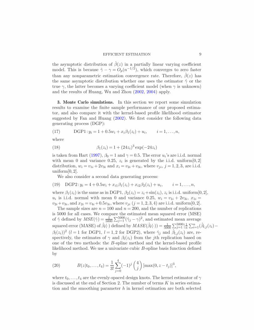
3. Monte Carlo simulations. In this section we report some simulationresults to examine the finite sample performance of our proposed estima-tor, and also compare it with the kernel-based profile likelihood estimatorsuggested by Fan and Huang (2002). We first consider the following datagenerating process (DGP):

DGP1 :yi = 1 + 0.5wi + xiβ1(zi) + ui, i = 1, . . . , n,(17)

where

β1(zi) = 1 + (24zi)3 exp(−24zi)(18)

is taken from Hart (1997), β0 = 1 and γ = 0.5. The error ui’s are i.i.d. normalwith mean 0 and variance 0.25, zi is generated by the i.i.d. uniform[0,2]distribution, wi = v1i +2v3i and xi = v2i + v3i, where vji, j = 1,2,3, are i.i.d.uniform[0,2].

We also consider a second data generating process:

DGP2 :yi = 4 + 0.5wi + xi1β1(zi) + xi2β2(zi) + ui, i = 1, . . . , n,(19)

where β1(zi) is the same as in DGP1, β2(zi) = zi+sin(zi), zi is i.i.d. uniform[0,2],ui is i.i.d. normal with mean 0 and variance 0.25, wi = v1i + 2v3i, x1i =v2i+v3i, and x2i = v4i+0.5v3i, where vji (j = 1,2,3,4) are i.i.d. uniform[0,2].

The sample sizes are n = 100 and n = 200, and the number of replicationsis 5000 for all cases. We compare the estimated mean squared error (MSE)of γ defined by MSE(γ) = 1

5000

∑5000j=1 (γj − γ)2, and estimated mean average

squared error (MASE) of βl(·) defined by MASE(βl(·)) = 15000

∑5000j=1 [ 1

n

∑ni=1(βl,j(zi)−

βl(zi))2 (l = 1 for DGP1, l = 1,2 for DGP2), where γj and βl,j(zi) are, re-

spectively, the estimates of γ and βl(zi) from the jth replication based onone of the two methods: the B-spline method and the kernel-based profilelikelihood method. We use a univariate cubic B-spline basis function definedby

B(z|t0, . . . , t4) =1

3!

4∑

j=0

(−1)j(

4j

)[max(0, z − tj)]

3,(20)

where t0, . . . , t4 are the evenly-spaced design knots. The kernel estimator of γis discussed at the end of Section 2. The number of terms K in series estima-tion and the smoothing parameter h in kernel estimation are both selected


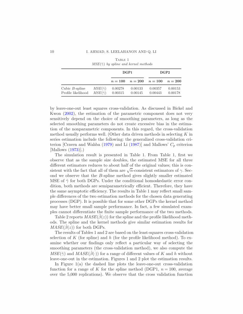
Table 1MSE (γ) by spline and kernel methods

DGP1 DGP2

n = 100 n = 200 n = 100 n = 200

Cubic B-spline MSE (γ) 0.00278 0.00133 0.00357 0.00153Profile likelihood MSE (γ) 0.00315 0.00145 0.00443 0.00178

by leave-one-out least squares cross-validation. As discussed in Bickel andKwon (2002), the estimation of the parametric component does not verysensitively depend on the choice of smoothing parameters, as long as theselected smoothing parameters do not create excessive bias in the estima-tion of the nonparametric components. In this regard, the cross-validationmethod usually performs well. (Other data driven methods in selecting K inseries estimation include the following: the generalized cross-validation cri-terion [Craven and Wahba (1979) and Li (1987)] and Mallows’ Cp criterion[Mallows (1973)].)

The simulation result is presented in Table 1. From Table 1, first weobserve that as the sample size doubles, the estimated MSE for all threedifferent estimators reduces to about half of the original values; this is con-sistent with the fact that all of them are

√n-consistent estimators of γ. Sec-

ond we observe that the B-spline method gives slightly smaller estimatedMSE of γ for both DGPs. Under the conditional homoskedastic error con-dition, both methods are semiparametrically efficient. Therefore, they havethe same asymptotic efficiency. The results in Table 1 may reflect small sam-ple differences of the two estimation methods for the chosen data generatingprocesses (DGP). It is possible that for some other DGPs the kernel methodmay have better small sample performance. In fact, a few simulated exam-ples cannot differentiate the finite sample performance of the two methods.

Table 2 reports MASE(β(z)) for the spline and the profile likelihood meth-ods. The spline and the kernel methods give similar estimation results forMASE(β(z)) for both DGPs.

The results of Tables 1 and 2 are based on the least-squares cross-validationselection of K (for spline) and h (for the profile likelihood method). To ex-amine whether our findings only reflect a particular way of selecting thesmoothing parameters (the cross-validation method), we also compute the

MSE (γ) and MASE(β(·)) for a range of different values of K and h withoutleave-one-out in the estimation. Figures 1 and 2 plot the estimation results.

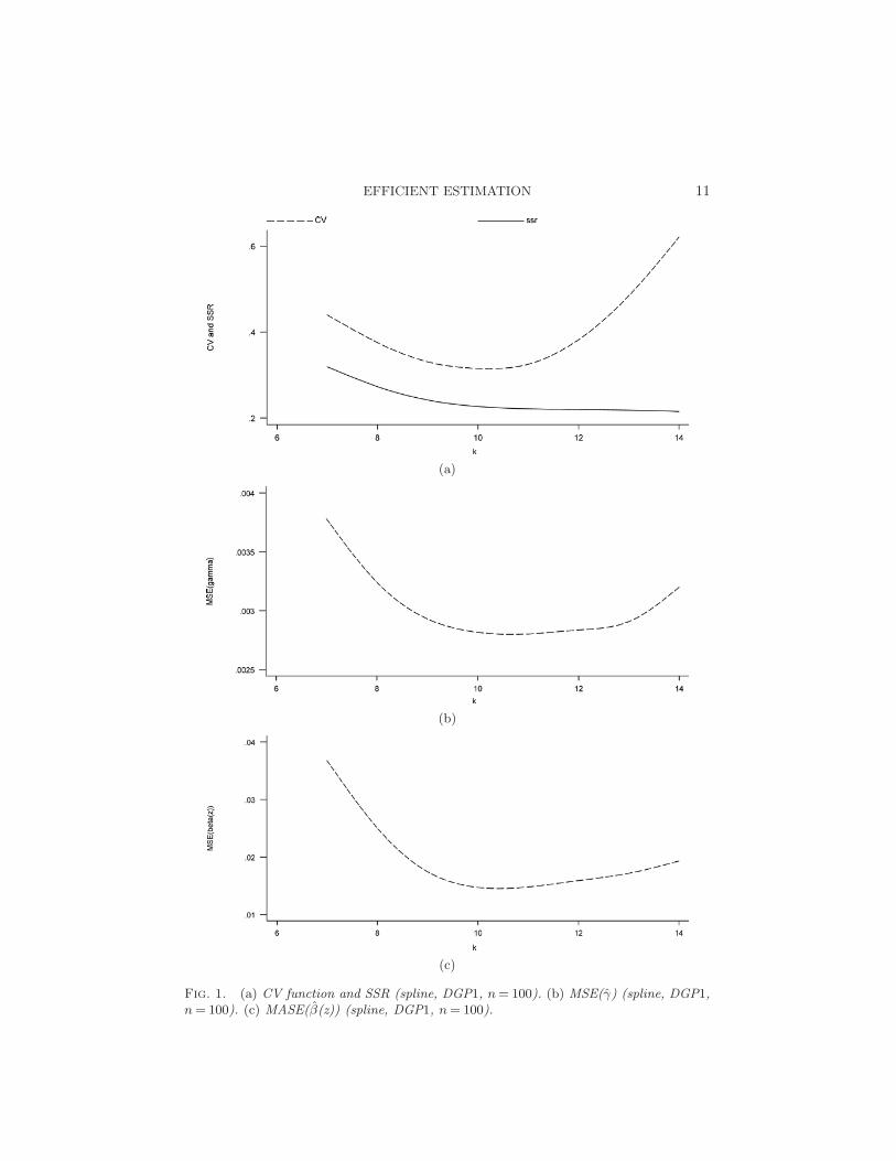
In Figure 1(a) the dashed line plots the leave-one-out cross-validationfunction for a range of K for the spline method (DGP1, n = 100, averageover the 5,000 replications). We observe that the cross validation function


(a)

(b)

(c)

Fig. 1. (a) CV function and SSR (spline, DGP1, n = 100). (b) MSE(γ) (spline, DGP1,n = 100). (c) MASE(β(z)) (spline, DGP1, n = 100).


(a)

(b)

(c)

Fig. 2. (a) CV function and SSR (kernel, DGP1, n = 100). (b) MSE(γ) (kernel, DGP1,n = 100). (c) MASE(β(z)) (kernel, DGP1, n = 100).


is minimized around K = 10. The solid line in Figure 1(a) is the sum ofsquared residuals computed without using the leave-one-out estimator; asexpected, it decreases as K increases.

Figure 1(b) graphs the MSE(γ) computed using all observations (not us-ing the leave-one-out method). We see that MSE (γ) takes minimum values

around K = 10 and K = 11. Figure 1(c) plots the MASE(β(z)), again com-

puted using all observations. MASE(β(z)) assumes minimum values aroundK = 10. The average of 5,000 cross-validation selected K’s is 10.42.

From Figure 1 we can see that, on average, the least squares cross-validation method performs well in selecting K that is close to values ofK that minimize MSE(γ) and MASE(β(z)). Note that both Figures 1(b)and 1(c) do not use the leave-one-out estimator. Therefore, unlike the sum of

squared residuals, MSE (γ) and MASE(β(z)) do not monotonically decreaseas K increases.

Figure 2 gives the corresponding cases for the profile kernel method.Figure 2(a) shows that the cross-validation function is minimized aroundh = 0.04, while the sum of squares of residuals monotonically increases withh.

Figures 2(b) and 2(c) show that both MSE(γ) and MASE(β(z)) are min-imized around h = 0.04. Note that Figures 2(b) and 2(c) are computed usingall observations (without using the leave-one-out method). Therefore, similar

to the spline case, MSE (γ) and MASE(β(z)) do not decrease monotonicallywith h, but rather they are both minimized around the value of h thatminimizes the cross-validation function.

Summarizing the results of Figures 1 and 2, we find that the cross-validation method performs adequately for the simulated data. The sim-ulation results reported in this section show that both the spline and thekernel methods can be a useful tool in estimating a partially linear varyingcoefficient model.

4. An empirical application. In this section we consider estimation ofa production function in China’s manufacturing industry to illustrate the

Table 2MASE(β(·)) by spline and kernel methods

DGP1 DGP2

MASE(β1(·)) MASE(β1(·)) MASE(β2(·))

n = 100 n = 200 n = 100 n = 200 n = 100 n = 200

Cubic B-spline 0.0162 0.00764 0.0576 0.0245 0.0635 0.0326Profile likelihood 0.0224 0.0110 0.0815 0.0356 0.0593 0.0318


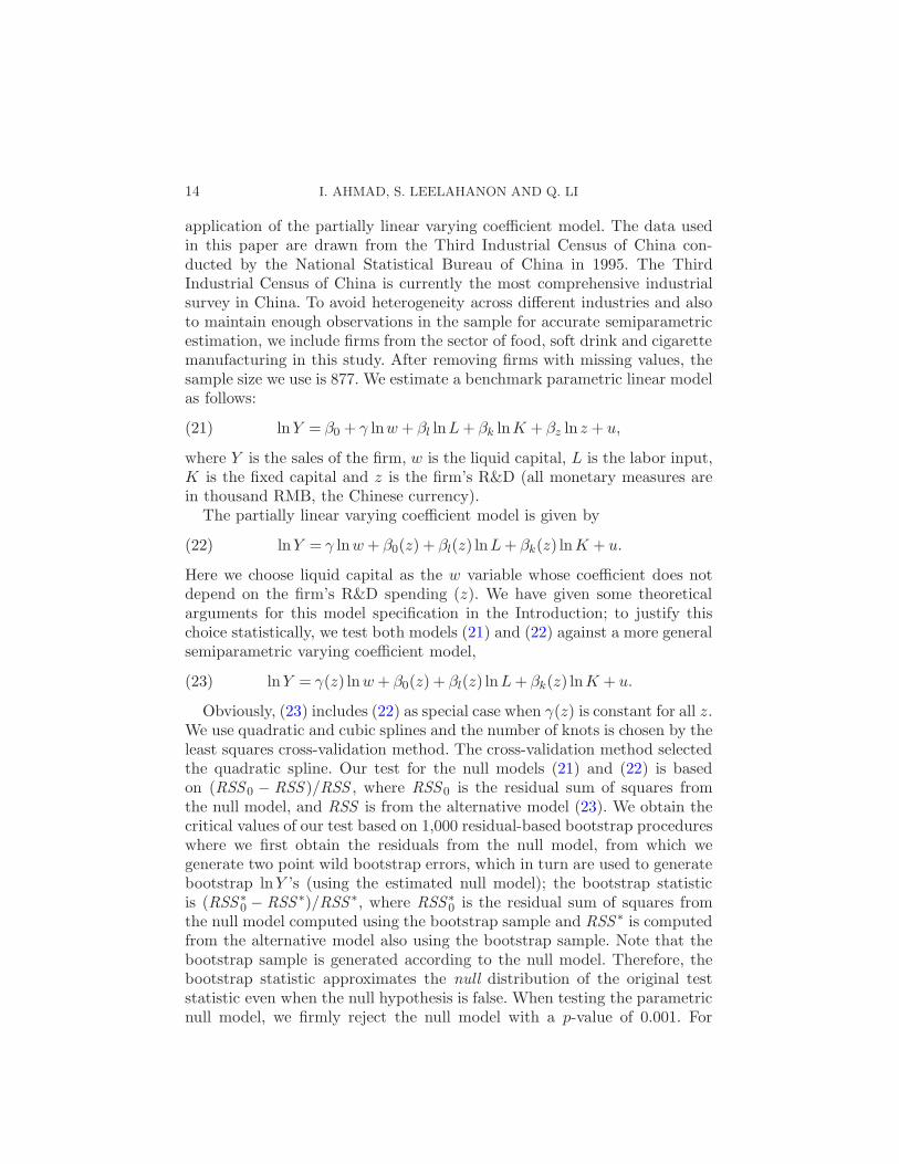
application of the partially linear varying coefficient model. The data usedin this paper are drawn from the Third Industrial Census of China con-ducted by the National Statistical Bureau of China in 1995. The ThirdIndustrial Census of China is currently the most comprehensive industrialsurvey in China. To avoid heterogeneity across different industries and alsoto maintain enough observations in the sample for accurate semiparametricestimation, we include firms from the sector of food, soft drink and cigarettemanufacturing in this study. After removing firms with missing values, thesample size we use is 877. We estimate a benchmark parametric linear modelas follows:

lnY = β0 + γ lnw + βl lnL + βk lnK + βz lnz + u,(21)

where Y is the sales of the firm, w is the liquid capital, L is the labor input,K is the fixed capital and z is the firm’s R&D (all monetary measures arein thousand RMB, the Chinese currency).

The partially linear varying coefficient model is given by

lnY = γ lnw + β0(z) + βl(z) lnL + βk(z) lnK + u.(22)

Here we choose liquid capital as the w variable whose coefficient does notdepend on the firm’s R&D spending (z). We have given some theoreticalarguments for this model specification in the Introduction; to justify thischoice statistically, we test both models (21) and (22) against a more generalsemiparametric varying coefficient model,

lnY = γ(z) lnw + β0(z) + βl(z) lnL + βk(z) lnK + u.(23)

Obviously, (23) includes (22) as special case when γ(z) is constant for all z.We use quadratic and cubic splines and the number of knots is chosen by theleast squares cross-validation method. The cross-validation method selectedthe quadratic spline. Our test for the null models (21) and (22) is basedon (RSS 0 − RSS )/RSS , where RSS 0 is the residual sum of squares fromthe null model, and RSS is from the alternative model (23). We obtain thecritical values of our test based on 1,000 residual-based bootstrap procedureswhere we first obtain the residuals from the null model, from which wegenerate two point wild bootstrap errors, which in turn are used to generatebootstrap lnY ’s (using the estimated null model); the bootstrap statisticis (RSS ∗

0 − RSS ∗)/RSS ∗, where RSS ∗0 is the residual sum of squares from

the null model computed using the bootstrap sample and RSS ∗ is computedfrom the alternative model also using the bootstrap sample. Note that thebootstrap sample is generated according to the null model. Therefore, thebootstrap statistic approximates the null distribution of the original teststatistic even when the null hypothesis is false. When testing the parametricnull model, we firmly reject the null model with a p-value of 0.001. For


testing the partially linear varying coefficient model (22), we cannot rejectthis null model at conventional levels (a p-value of 0.162). Therefore, botheconomic theory and the statistical testing results support our specification(22).

The estimated value of γ based on (22) is 0.481, with a standard errorof 0.0372 (the t-statistic is 12.91). The goodness-of-fit R2 is 0.566 [R2 =1−RSS/

∑i(yi− y)2, yi = lnYi]. The estimated varying coefficient functions

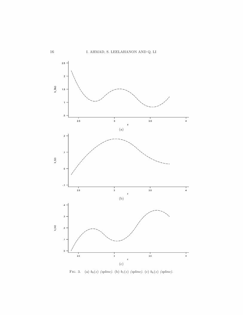
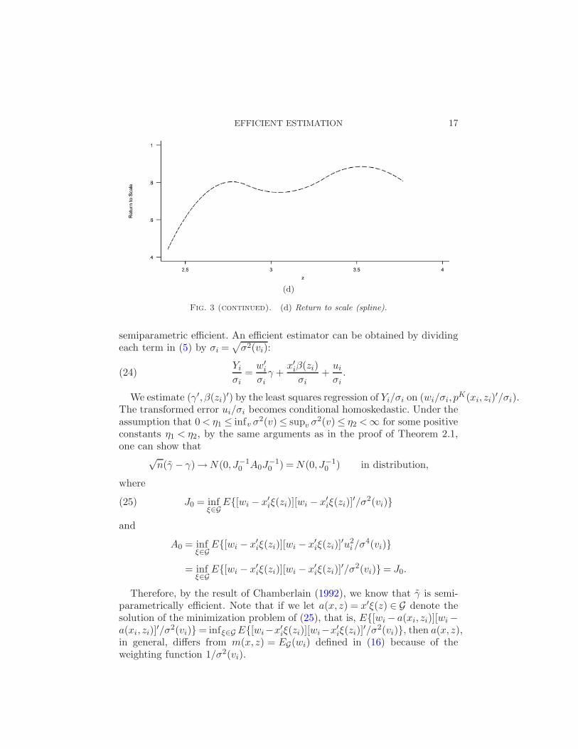
are plotted in Figures 3(a) to 3(c). β0(z) is plotted in Figure 3(a). Figure 3(b)shows that the marginal productivity of labor βl(z) is a nonlinear function ofz (R&D). The marginal productivity of labor first increases with z and thendecreases as z increases further. The bell shape of the curve suggests that,while modest R&D can improve labor productivity, higher R&D leads tolower labor productivity. Figure 3(c) shows that the marginal productivityof (fixed) capital is also nonlinear in z. It exhibits a general up trend with z,indicating that firms with large R&D spending yield relative higher marginal(fixed) capital productivity. These results are not surprising given that mostof the firms in our sample are state-owned. It is typical in these firms thatcapital is scarce while labor is excessive. Thus, most of the R&D expenses areused to improve equipment performance, but not to train labor. In Figure3(d) we graph the return to scale function γ + βl(z) + βk(z). The return toscale is well below one (the constant return to scale level) for firms withsmall R&D, and it increases to a range between 0.8 to 0.9 for firms withlarge R&D expenditures. The results indicate that most of the firms in oursample exhibit decreasing returns to scale in production. It partly reflects thefact that the firms included in the survey are large firms, most of which arestate-owned firms. These firms typically have a production scale larger thanideal. In particular, there are usually too many employees in these firms. Itwas not until several years after the survey we use in this paper, as a resultof fierce competition from foreign firms and the passage of bankruptcy lawin China, that the food, soft drink and cigarette sector witnessed a string ofreorganizations, mergers and acquisitions. Further discussion is beyond thescope of this paper.

We have also applied the kernel profile likelihood method to this dataset. The estimation results are quite similar to those obtained by the splinemethod. For example, the estimated γ is 0.489 with a t-statistic of 13.20.The β(z) functions all have similar shapes as those obtained by the splinemethod. Therefore, we do not report the kernel estimation results here.

5. Possible extension. In this section we briefly discuss (without provid-ing technical details) efficient estimation of a partially varying coefficientmodel when the error is conditional heteroskedastic.

Theorem 2.1 holds even when the error is conditional heteroskedastic,say, E(u2

i |vi) = σ2(vi), where vi = (wi, xi, zi). However, in this case γ is not


(a)

(b)

(c)

Fig. 3. (a) b0(z) (spline). (b) b1(z) (spline). (c) bk(z) (spline).


(d)

Fig. 3 (continued). (d) Return to scale (spline).

semiparametric efficient. An efficient estimator can be obtained by dividingeach term in (5) by σi =

√σ2(vi):

Yi

σi=

w′i

σiγ +

x′iβ(zi)

σi+

ui

σi.(24)

We estimate (γ′, β(zi)′) by the least squares regression of Yi/σi on (wi/σi, p

K(xi, zi)′/σi).

The transformed error ui/σi becomes conditional homoskedastic. Under theassumption that 0 < η1 ≤ infv σ2(v) ≤ supv σ2(v) ≤ η2 <∞ for some positiveconstants η1 < η2, by the same arguments as in the proof of Theorem 2.1,one can show that

√n(γ − γ)→ N(0, J−1

0 A0J−10 ) = N(0, J−1

0 ) in distribution,

where

J0 = infξ∈G

E[wi − x′iξ(zi)][wi − x′

iξ(zi)]′/σ2(vi)(25)

and

A0 = infξ∈G


iξ(zi)]′u2

i /σ4(vi)

= infξ∈G


iξ(zi)]′/σ2(vi)= J0.

Therefore, by the result of Chamberlain (1992), we know that γ is semi-parametrically efficient. Note that if we let a(x, z) = x′ξ(z) ∈ G denote thesolution of the minimization problem of (25), that is, E[wi − a(xi, zi)][wi −a(xi, zi)]

′/σ2(vi) = infξ∈G E[wi−x′iξ(zi)][wi−x′

iξ(zi)]′/σ2(vi), then a(x, z),

in general, differs from m(x, z) = EG(wi) defined in (16) because of theweighting function 1/σ2(vi).


It is unlikely that σ2(vi) is known in practice. Let σ2(vi) denote a genericnonparametric estimator of σ2(vi), and write σi =

√σ2(vi). Then one can ob-

tain feasible estimators for γ and β(z) by regressing Yi/σi on [w′i/σi, p

K(xi, zi)/σi].The resulting estimator of γ will be semiparametric efficient provided thatσ(v) converges to σ(v) uniformly with a certain rate for all v in the compactsupport of v.

For the kernel-based profile likelihood approach, it is more difficult toobtain efficient estimation when the error is conditional heteroskedastic.Recall that EG(Ai) denotes the projection of Ai on the varying coefficientfunctional space G. From (5) we have

yi −EG(yi) = (wi −EG(wi))′γ + ui.(26)

Dividing each term in (26) by σi, we get

yi −EG(yi)

σi=

(wi −EG(wi))′

σiγ +

ui

σi.(27)

Let γ denote the least squares estimator of γ based on (27). By the Lin-deberg central limit theorem, we have

√n(γ − γ) → N(0,E[(wi −EG(wi))(wi −EG(wi))

′/σ2i ]−1)

(28)in distribution.

However, γ is not semiparametrically efficient because

E[(wi −EG(wi))(wi −EG(wi))′/σ2

i ]

6= infg∈G

E[(wi − g(xi, zi))(wi − g(xi, zi))′/σ2(vi)]

due to the weight function 1/σ2i . [EG(wi) is defined as the (un-weighted) pro-

jection of wi on the varying coefficient functional space G. It differs from theweighted projection in general.] We conjecture that some iterative procedure(similar to the backfitting algorithm) is needed in order to obtain an efficientkernel-based estimator for γ when the error is conditional heteroskedastic.

APPENDIX

Throughout this Appendix, C denotes a generic positive constant thatmay be different in different uses,

∑i =

∑ni=1. The norm ‖ · ‖ for a matrix

A is defined by ‖A‖ = [tr(A′A)]1/2. Also, when A is a matrix and an is apositive sequence depending on n, A = Op(an) [or op(an)] means that eachelement of A is Op(an) [or op(an)]. Also, when we write A≤ C for a constantscalar C, it means that each element of A is less or equal to C.

Proof of Theorem 2.1. Recall that θ(xi, zi) = E[wi|xi, zi], m(xi, zi) =EG(wi) = EG(θ(xi, zi)) and εi = wi − m(zi, xi). Define vi = wi − θ(xi, zi)


and ηi = θ(zi, xi) − m(xi, zi). We will use the following short-hand nota-tion: θi = θ(xi, zi), gi = x′

iβ(zi) and mi = m(xi, zi). Hence, vi = wi − θi,εi = θi + vi − mi, ηi = θi −mi. Finally, the variables without subscript rep-resent matrices, for example, θ = (θ1, . . . , θn)′ is of dimension n× 1.

Also recall that for any matrix A with n rows, we define A = P (P ′P )−P ′A[P is defined below (6)]. Applying this definition to θ,m, g, η, u, v, we getθ, m, g, η, u, v.

Since wi = θi + vi and θi = mi + ηi, we get wi = ηi + vi + mi and wi =ηi + vi + mi. In matrix notation,

W = η + v + m and W = η + v + m.

Therefore, we have

W − W = η + v + (m− m)− v − η.(29)

For scalars or column vectors Ai and Bi, we define SA,B = n−1∑i AiB

′i

and SA = SA,A. We also define the scalar function SA = n−1∑i A

′iAi, which

is the sum of the diagonal elements of SA. Using ab ≤ (a2 + b2)/2, it iseasy to see that each element of SA,B is less or equal to SA + SB . Whenwe evaluate the probability order of SA,B, we often write SA,B ≤ SA + SB .The scalar bound SA + SB bounds each of the elements in SA,B . There-fore, if SA + SB = Op(an) (for some sequence an), then each element ofSA,B is at most Op(an), which implies that SA,B = Op(an). Similarly, using

the Cauchy–Schwarz inequality, we have SA,B ≤ (SASB)1/2. Here again, thescalar bounds all the elements in SA,B .

Note that if S−1

W−Wexists, then, from (10) and (11), we get

√n(γ − γ) =

[n−1

∑

i

(wi − wi)(wi − wi)′

]−1

(30)×√

n

n−1

∑

i

(wi − wi)(gi − gi + ui − ui)

= S−1

W−W

√nS

W−W ,g−g+u−u,

where gi = x′iβ(zi).

For the first part of the theorem, we will prove the following: (i) SW−W

=

Φ+op(1), (ii) SW−W ,g−g

= op(n−1/2), (iii) S

W−W ,u= op(n

−1/2) and (iv)√

nSW−W ,u

→N(0,Ω) in distribution.

Proof of (i). For a matrix A and scalar sequence an, A = Op(an)(op(an)) means that each element of A has an order of Op(an) (op(an)).Using (29), we have

SW−W

= Sη+v+(m−m)−v−η = Sη+v + S(m−m)−v−η + 2Sη+v,(m−m)−v−η.(31)


The first term Sη+v = 1n

∑i(ηi + vi)(ηi + vi)

′ = 1n

∑i εiε

′i = Φ + op(1) by

virtue of the law of large numbers.The second term S(m−m)−v−η ≤ 3(S(m−m) + Sv + Sη) = op(1) by Lemmas

A.3, A.4(i) and A.5, stated and proved at the end of this Appendix.The last term Sη+v,(m−m)−v−η ≤ Sη+vS(m−m)−v−η1/2 = (Op(1)op(1))

1/2 =op(1) by the preceding results, where for an m × m matrix A, Diag(A) is

an m × 1 matrix with the diagonal elements of A, and A1/2 has the samedimension as A by taking the square root for each element of A.

Proof of (ii). Using (29), we have

SW−W ,g−g

= Sη+v+(m−m)−v−η,g−g

(32)= Sη+v,g−g + Sm−m,g−g − Sv,g−g − Sη,g−g.

For the first term, by noting that ηi + vi is orthogonal to the vary-ing coefficient functional space G, and gi − gi belong to G, we have us-ing Lemma A.3, E[‖Sη+v,g−g‖2] = n−2∑n

i=1 E[(ηi + vi)(ηi + vi)′(gi − gi)

2] ≤Cn−1(

∑dl=1 k2δl

l )×E[‖η1 +v1‖2] = O(n−1∑dl=1 k2δl

l ) = o(n−1), which implies

that Sη+v,g−g = Op(n−1/2∑d

l=1 k−δl

l ).

The second term Sm−m,g−g ≤ (Sm−mSg−g)1/2 = Op(

∑dl=1 k−2δl

l ) by Lem-ma A.3.

The third term Sv,g−g ≤ (S vSg−g)1/2 = Op((K/n)1/2)Op(

∑dl=1 k−δl

l ) by

Lemmas A.3 and A.4(i). The last term Sη,g−g ≤ (S ηSg−g)1/2 = Op((k/n)1/2)×

Op(∑d

l=1 k−δl

l ) by Lemmas A.3 and A.5.

Combining the above four terms we have SW−W ,g−g

= Op((n−1/2+(K/n)1/2)(

∑dl=1 k−δl

l )+∑d

l=1 k−2δl

l ) = op(n−1/2) by Assumption 2.3.

Proof of (iii). Using (29), we have

SW−W ,u

= Sη+v+(m−m)−v−η,u = Sη+v,u + Sm−m,u − Sv,u − Sη,u.(33)

The first term Sη+v,u ≤ (Sη+vSu)1/2 = Op(K/n) by Lemma A.4(ii). The

second term Sm−m,u ≤ (Sm−mSu)1/2 = Op(∑d

l=1 k−δl

l )Op(√

K/√

n ) by Lem-mas A.3 and A.4(ii).

The third term Sv,u ≤ (S vSu)1/2 = Op(K/n) by Lemma A.4(i), (ii). The

last term Sη,u ≤ (SηSu)1/2 = Op(K/n) by Lemmas A.4(ii) and A.5.

Combining all four terms, we get SW−W ,u

= Op(K/n+n−1/2∑dl=1 k−δl

l ) =

op(n−1/2) by Assumption 2.3.

Proof of (iv). Using (29), we have√

nSW−W ,u

=√

nSη+v+(m−m)−v−η,u

(34)=√

nSη+v,u +√

n(Sm−m,u − Sv,u − Sη,u).


The first term√

nSη+v,u =√

n∑n

i=1(ηi + vi)ui =√

n∑n

i=1 εiui → N(0,Ω)in distribution by the Lindeberg–Feller central limit theorem.

The second term E[S2m−m,u|X,Z] = 1

n2 tr(m−m)(m−m)′E[uu′|X,Z] ≤(C/n) tr[(m−m)′(m−m)/n] = (C/n)Sm−m = op(n

−1) by Lemma A.3. Hence,

Sm−m,u = op(n−1/2).

The third term E[S2v,u|X,Z] = 1

n2 tr(P (P ′P )−1P ′vv′P (P ′P )−1P ′E[uu′|X,Z]) ≤(C/n2) tr[P (P ′P )−1P ′vv′P (P ′P )−1P ′] = (C/n) tr(vv′/n) = (C/n)Sv = op(n

−1)

by Lemma A.4(i). Hence, Sv,u = op(n−1/2).

The last term Sη,u = op(n−1/2) by the same proof as Sv,u = op(n

−1/2) byciting Lemma A.5, rather than citing Lemma A.4(i).

Combining proofs of (i)–(iv) with (30), we conclude that√

n(γ − γ) →N(0,Φ−1ΩΦ−1) in distribution.

For the second part of the theorem, we need to show that Σ = Σ + op(1),

where Σ = Φ−1ΩΦ−1. But Φ = SW−W

= Φ + op(1) is proved in the proof

of (i) above. By a similar argument, it is easy to show that Ω = Ω + op(1).

Therefore, Σ = Σ + op(1).

Proof of Theorem 2.2. We will prove Theorem 2.2 by replacingβ(z) and β(z) by g(x, z) = x′β(z) and g(x, z) = x′β(z), respectively, because

|g(x, z)− g(x, z)|2 = |x′(β(z)−β(z))|2 ≤ d∑d

l=1 x2l (βl(z)−βl(z))2, which has

the same order as ‖β(z) − β(z)‖2 under the bounded support assumption.Hence, the rate of convergence for g(x, z) − g(x, z) is the same as that of

β(z)− β(z).The proof is similar to the proof of Theorem 1 in Newey (1997). Define an

indicator function 1n which equals 1 if (P ′P ) is nonsingular and 0 otherwise.We first find the convergence rate of 1n‖α − α‖. By (12) and (7), and if(P ′P )−1 exists, we have

α = (P ′P )−1P ′(Y −Wγ)

= (P ′P )−1P ′(Y −Wγ −W (γ − γ))

= (P ′P )−1P ′(Pα + (G− Pα) + u−W (γ − γ))(35)

= α + (P ′P/n)−1P ′(G−Pα)/n + (P ′P/n)−1P ′u/n

− (P ′P/n)−1P ′W (γ − γ)/n.

Hence,

1n‖α− α‖ ≤ 1n‖(P ′P/n)−1P ′(G−Pα)/n‖

+ 1n‖(P ′P/n)−1P ′u/n‖(36)

+ 1n‖(P ′P/n)−1P ′W (γ − γ)/n‖.


The first term 1n‖(P ′P/n)−1P ′(G − Pα)/n‖ = Op(∑d

l=1 k−δl

l ) by Lem-ma A.2.

The second term

E[1n‖(P ′P/n)−1P ′u/n‖|X,Z]

= 1nE[((u′P/n)(P ′P/n)−1(P ′P/n)−1(P ′u/n))1/2|X,Z]

≤ Op(1)1n tr(P (P ′P )−1P ′E[uu′|X,Z]/n)1/2

≤ Op(1)1nC√

K/√

n

by Lemma A.1 and Assumption 2.1. Hence, 1n‖(P ′P/n)−1P ′u/n‖ = Op(√

K/√

n ).As for the last term, note that W = η + v + m = ε + m and γ − γ =

Op(n−1/2) by Theorem 2.1. Therefore,

E[1n‖(P ′P/n)−1P ′W/n‖|X,Z]

= 1nE[‖(P ′P/n)−1P ′(ε + m)/n‖|X,Z]

≤ 1nE[‖(P ′P/n)−1P ′ε/n‖|X,Z] + 1nE[‖(P ′P/n)−1P ′m/n‖|X,Z].

Also,

1nE[‖(P ′P/n)−1P ′ε/n‖|X,Z]

= 1nE[‖(ε′P/n)(P ′P/n)−1(P ′P/n)−1(P ′ε/n)‖|X,Z]

≤Op(1)1n tr(P (P ′P )−1P ′E[εε′|X,Z]/n)1/2

≤Op(1)1nC√

K/√

n

by Lemma A.1 as in the proof of Theorem 2.1. Hence, 1n|(P ′P/n)−1P ′ε/n|=Op(

√K/

√n ) = op(1).

1n‖(P ′P )−1P ′m‖= 1n‖(P ′P/n)−1P ′m/n‖= Op(1) by Lemma A.2.Combining the above results, also noting that 1n → 1 almost surely, we

have

‖α− α‖ = Op

(d∑

l=1

k−δl

l +√

K/√

n

).(37)

To prove part (i) of Theorem 2.2, using (37) and Assumption 2.3, and

also noting that g(x, z) = x′β(z) = pK(x, z)′α, we have

sup(x,z)∈S

|g(x, z)− g(x, z)| ≤ sup(x,z)∈S

|pK(x, z)′(α− α)|+ |pK(x, z)′α− g(x, z)|

≤ ζ0(K)‖α− α‖+ O

(d∑

l=1

k−δl

l

)


= Op

(ζ0(K)

(d∑

l=1

k−δl

l +√

K/√

n

)).

Proofs for (ii) and (iii) are similar, and we only prove (ii),

n−1n∑

i=1

[g(xi, zi)− g(zi, zi)]2

= n−1‖Pα−G‖2

≤ 2n−1‖P (α −α)‖2 + ‖Pα−G‖2= 2(α−α)′(P ′P/n)(α−α) + 2 sup

(x,z)∈S[pK(x, z)α− g(x, z)]2

= Op

(K/n +

d∑

l=1

k−2δl

l

)

by (37), Lemma A.1 and Assumption 2.3(i). Thus, we have proved Theorem2.2.

We now present some lemmas that are used in the proofs of Theorems 2.1and 2.2. We will omit the indicator function 1n below since Prob(1n = 1) → 1almost surely. Following the arguments in Newey (1997), we can assumewithout loss of generality that B = I (B is defined in Assumption 2.2).Hence, PK(X,Z) = pK(X,Z), and Q = E[pK(xi, zi)p

K(xi, zi)′] = I (I is an

identity matrix of dimension K); see Newey (1997) for the reasons and morediscussion of these issues. Recall that pK(x, z) is a K ×1 matrix and rewriteeach component of this matrix as pK(x, z) = (p1K(x, z), . . . , pKK(x, z))′.

Lemma A.1. ‖Q− I‖ = Op(ζ0(K)√

K/√

n ) = op(1), where Q = P ′P/n.

Proof. This is Theorem 1 in Newey (1997).

Lemma A.2. ‖αf −αf‖ = Op(∑d

l=1 k−δl

l ), where αf = (P ′P )−1P ′f , αf sat-

isfies Assumption 2.3 and f = G or f = m.

Proof. By Lemma A.1, Assumption 2.3 and the fact that P (P ′P )−1P ′

is idempotent,

‖αf −αf‖ = ‖(P ′P )−1P ′(f −Pαf )‖

= ‖(f − Pαf )′P (P ′P )−1QP ′(f −Pαf )/n‖1/2

≤ Op(1)‖(f −Pαf )′P (P ′P )−1P ′(f −Pαf )/n‖1/2


≤ Op(1)‖(f −Pαf )′(f −Pαf )/n‖1/2 = Op

(d∑

l=1

k−δl

l

).

Lemma A.3. Sf−f = Op(∑d

l=1 k−2δl

l ), where f = G or f = m.

Proof. Note that f = Pαf . By Assumption 2.3 and Lemmas A.1 andA.2,

Sf−f =1

n|f − f |2 ≤ 1

n(|f − Pαf |2 + |P (αf − αf )|2)

= O

(d∑

l=1

k−2δl

l

)+ (αf − αf )′(P ′P/n)(αf − αf )

≤ O

(d∑

l=1

k−2δl

l

)+ Op(1)|αf − αf |2 = Op

(d∑

l=1

k−2δl

l

).

Lemma A.4. (i) Sv = Op(K/n), (ii) Su = Op(K/n).

Proof. (i) This proof is similar to the proof of Theorem 1 of Newey(1997),

E[Sv|X,Z] =1

nE[v′P (P ′P )−1P ′v|X,Z]

=1

nE[tr(P (P ′P )−1P ′E[vv′|X,Z])]

≤ C

ntr(P (P ′P )−1P ′) = C

(K

n

).

Hence, Sv = Op(K).(ii) follows as in the proof of Lemma A.4(i).

Lemma A.5. Sη = Op(K/n).

Proof. First we show that (P ′η/n) = Op(√

K/√

n ). Recall that θ(xi, zi) =E(wi|xi, zi) and ηi = θ(xi, zi) − EG [θ(xi, zi)]. Note that pK(xi, zi) ∈ G andEG(ηi) = 0 (i.e., η ⊥G). Hence, E‖P ′η/n‖2 = n−2∑

i E[pK(xi)′‖ηi‖2pK(xi)]≤

Cn E[pK(Xi)

′pK(xi)] = Cn trE[pK(Xi)p

K(xi)′] = (CK/n) = O(K/n), which

implies that (P ′η/n) = Op(√

K/√

n ).Thus, Sη = n−1η′η = (η′P/n)(P ′P/n)−1(P ′η/n) = Op(K/n)Op(1) = Op(K/n)

by Lemma A.1 and the fact that P ′η/n = Op(√

K/√

n ) as shown above.


Acknowledgments. We are grateful for the insightful comments from tworeferees and an Associate Editor which greatly improved the paper. Wewould also like to thank Dong Li for his help in the empirical work of thispaper.

REFERENCES

Ai, C. and Chen, X. (2003). Efficient estimation of models with conditional momentrestrictions containing unknown functions. Econometrica 71 1795–1843. MR2015420

Andrews, D. W. K. (1991). Asymptotic normality of series estimators for nonparametricand semiparametric regression models. Econometrica 59 307–345. MR1097531

Bickel, P. J., Klaassen, C. A. J., Ritov, Y. and Wellner, J. A. (1993). Efficient andAdaptive Inference for Semiparametric Models. Johns Hopkins Univ. Press. MR1245941

Bickel, P. J. and Kwon, J. (2002). Inference for semiparametric models: Some currentfrontiers and an answer (with discussion). Statist. Sinica 11 863–960. MR1867326

Cai, Z., Fan, J. and Li, R. (2000). Efficient estimation and inferences for varying-coefficient models. J. Amer. Statist. Assoc. 95 888–902. MR1804446

Cai, Z., Fan, J. and Yao, Q. (2000). Functional-coefficient regression models for nonlineartime series. J. Amer. Statist. Assoc. 95 941–956. MR1804449

Carroll, R. J., Fan, J., Gijbels, I. and Wand, M. P. (1997). Generalized partiallylinear single-index models. J. Amer. Statist. Assoc. 92 477–489. MR1467842

Chamberlain, G. (1992). Efficiency bounds for semiparametric regression. Econometrica60 567–596. MR1162999

Chen, R. and Tsay, R. S. (1993). Functional-coefficient autoregressive models. J. Amer.Statist. Assoc. 88 298–308. MR1212492

Craven, P. and Wahba, G. (1979). Smoothing noisy data with spline functions: Esti-mating the correct degree of smoothing by generalized cross-validation. Numer. Math.31 377–403. MR516581

Fan, J. and Huang, L.-S. (2001). Goodness-of-fit tests for parametric regression models.J. Amer. Statist. Assoc. 96 640–652. MR1946431

Fan, J. and Huang, T. (2002). Profile likelihood inferences on semiparametric varying-coefficient partially linear models. Unpublished manuscript.

Fan, J., Yao, Q. and Cai, Z. (2003). Adaptive varying-coefficient linear models. J. R.Stat. Soc. Ser. B Stat. Methodol. 65 57–80. MR1959093

Fan, J. and Zhang, W. (1999). Statistical estimation in varying coefficient models. Ann.Statist. 27 1491–1518. MR1742497

Green, P. J. and Silverman, B. W. (1994). Nonparametric Regression and Gener-alized Linear Models: A Roughness Penalty Approach. Chapman and Hall, London.MR1270012

Hardle, W., Liang, H. and Gao, J. (2000). Partially Linear Models. Physica-Verlag,Heidelberg. MR1787637

Hart, J. (1997). Nonparametric Smoothing and Lack-of-fit Tests. Springer, New York.MR1461272

Hastie, T. and Tibshirani, R. (1993). Varying coefficient models (with discussion).J. Roy. Statist. Soc. Ser. B 55 757–796. MR1229881

Hoover, D. R., Rice, J. A., Wu, C. O. and Yang, L.-P. (1998). Nonparametric smooth-ing estimates of time-varying coefficient models with longitudinal data. Biometrika 85

809–822. MR1666699Huang, J. Z. (1998). Projection estimation in multiple regression with application to

functional ANOVA models. Ann. Statist. 26 242–272. MR1611780

http://www.ams.org/mathscinet-getitem?mr=2015420




















Huang, J. Z. (2003). Local asymptotics for polynomial spline regression. Ann. Statist. 31

1600–1635. MR2012827Huang, J. Z., Wu, C. O. and Zhou, L. (2002). Varying coefficient models and basis

function approximations for the analysis of repeated measurements. Biometrika 89 111–128. MR1888349

Huang, J. Z., Wu, C. O. and Zhou, L. (2004). Polynomial spline estimation and infer-ence for varying coefficient models with longitudinal data. Statist. Sinica 14 763–788.MR2087972

Li, K. C. (1987). Asymptotic optimality for Cp, CL, cross-validation and generalizedcross-validation: Discrete index set. Ann. Statist. 15 958–975. MR902239

Li, Q., Huang, C. J., Li, D. and Fu, T.-T. (2002). Semiparametric smooth coefficientmodels. J. Bus. Econom. Statist. 20 412–422. MR1939909

Lorentz, G. G. (1966). Approximation of Functions. Holt, Rinehart and Winston, NewYork. MR213785

Mallows, C. L. (1973). Some comments on Cp. Technometrics 15 661–675.Newey, W. K. (1997). Convergence rates and asymptotic normality for series estimators.

J. Econometrics 79 147–168. MR1457700Robinson, P. M. (1988). Root-N-consistent semiparametric regression. Econometrica 56

931–954. MR951762Shen, X. (1997). On methods of sieves and penalization. Ann. Statist. 25 2555–2591.

MR1604416Speckman, P. (1988). Kernel smoothing in partially linear models. J. Roy. Statist. Soc.

Ser. B 50 413–436. MR970977Stock, C. J. (1989). Nonparametric policy analysis. J. Amer. Statist. Assoc. 89 567–575.

MR1010347Xia, Y. C. and Li, W. K. (1999). On the estimation and testing of functional-coefficient

linear models. Statist. Sinica 9 735–758. MR1711643Xia, Y. C. and Li, W. K. (2002). Asymptotic behavior of bandwidth selected by the

cross-validation method for local polynomial fitting. J. Multivariate Anal. 83 265–287.MR1945954

Zhang, W., Lee, S.-Y. and Song, X. (2002). Local polynomial fitting in semivaryingcoefficient models. J. Multivariate Anal. 82 166–188. MR1918619

Zhou, S., Shen, X. and Wolfe, D. A. (1998). Local asymptotics for regression splinesand confidence regions. Ann. Statist. 26 1760–1782. MR1673277

I. AhmadDepartment of StatisticsUniversity of Central FloridaOrlando, Florida 32816-2370USAe-mail: [email protected]

S. LeelahanonFaculty of EconomicsThammasat University2 Pra Chan RoadBangkok 10200Thailand

Q. LiDepartment of EconomicsTexas A&M UniversityCollege Station, Texas 77843-4228USA
















mailto:[email protected]

Efficient estimation of a semiparametric partially linear varying coefficient model

Documents