Effects of a Low-Velocity Zone on a Dynamic Rupture

Bulletin of the Seismological Society of America, Vol. 87, No. 5, pp. 1267-1280, October 1997

Effects of a Low-Velocity Zone on a Dynamic Rupture

by Ruth A. Harris and Steven M. Day

Abstract Dynamic-crack earthquake simulations generally assume that the crustal material surrounding faults is laterally homogeneous. Tomographic and near-fault seismic studies indicate that the crust near faults is instead comprised of rocks of varying material velocities. We have tested the effects of adding material-velocity variation to simulations of spontaneously propagating earthquakes. We used two- dimensional plane strain conditions coupled with a slip-weakening fracture criterion and examined earthquakes on faults that bisect finite-width low-velocity zones embedded in country rock and earthquakes on faults that bound two different-velocity materials. When a fault bisects a low-velocity zone, the normal stress remains un- changed, but both the rupture velocity and slip-velocity pulse shape are perturbed. The presence of the low-velocity zone induces high-frequency oscillations in the slip function near the rupture front. When the fault is on the edge of the low-velocity zone, the oscillations are more pronounced, and repeated sticking and slipping can occur near the rupture front. For the slip-weakening (velocity-independent) friction model, however, the temporary sticking does not lead to permanent arrest of slip, and slip duration is still controlled by the overall rupture dimension. When an earthquake ruptures a fault juxtaposing a lower-velocity material against a higher-velocity material, the normal stress across the fault near the crack tip is perturbed. The sign of the normal stress perturbation depends on the direction of rupture, leading in some cases to a directional dependence of rupture velocity. When slip is accompanied by stress reduction, a positive feedback develops between the normal and shear stress changes, as previously noted by Andrews and Ben-Zion (1997), resulting in an ap- parerltly unavoidable grid-size dependence in computation of stress change near the rupture front. Numerical experiments indicate, however, that the rupture velocity is insensitive to this zone size dependence, which is highly localized immediately behind the crack tip. The factors controlling the rupture velocity in the simulations, including directional dependence, are further elucidated by a new analytical solution for rupture of an asperity on a frictionless interface.

Introduction

Numerical simulations of earthquakes provide significant insights into earthquake rupture dynamics and facilitate the physical interpretation of the kinematic earthquake models derived from seismic recordings. For example, numerical simulations have clarified the relationship between slip rise time and gross fault dimension (e.g., Madariaga, 1976; Day, 1982a) for simple ruptures and have demonstrated the important influence on rise time introduced by secondary length scales such as asperity dimensions (Mikumo and Mi- yatake, 1987; Beroza and Mikumo, 1996; Day et al., 1996). Such simulations have also demonstrated how rupture velocity changes can occur in response to heterogeneities of strength and stress drop.

To date, most dynamic simulations have considered only simplified models of faulting in which the fault is a

smooth, planar surface embedded in a uniform elastic medium. Harris et al. (1991) and Harris and Day (1993) relaxed this restriction somewhat to treat rupture of faults with non- coplanar segments. They delineated conditions required to trigger multi-segment earthquakes. They also showed that in such earthquakes, stress transfer at segment boundaries can give rise to rupture delays comparable to those imaged from seismic observations, as in, for example, Campillo and Ar- chuleta's (1993) and Wald and Heaton's (1994) studies of the 1992 Landers earthquake.

In the present study, we consider potential effects on earthquake dynamics introduced when the seismic velocity near a fault is discontinuous. In particular, we consider rupture of a fault embedded in a low-velocity zone (LVZ). We focus attention on two special cases of the low-velocity zone

1267

1268 R.A. Harris and S. M. Day

problem that have been shown by seismic studies to be geologically important, and which arise naturally in fault zones. The first is the case in which the fault is embedded in a narrow, fanlt-parallel low-velocity zone with width of the order of a few hundred meters. Such zones are too narrow to be readily identified using transmitted seismic waves. Recently, narrow low-velocity zones have been identified along numerous strike-slip faults with the aid of fault-zone trapped modes (Li et al., 1990, 1994a, 1994b, 1995; Hough et al., 1994). They indicate the presence of a zone of altered rock and fault gouge generated from past rupture events. Quantitative estimates of the velocity contrast and width of these low-velocity zones have been obtained from the observed dispersion of the trapped waves (e.g., Li and Vidale, 1996), and it appears plausible that the presence of these LVZs may have a significant effect on rupture dynamics. We simulate rupture of faults that bisect the low-velocity zone as well as of those that localize along its contact with un- disturbed "country" rock.

The second special case of particular interest is the lim- iting case in which the low-velocity zone width is infinite, and rupture is on the interface between two half-spaces of contrasting seismic velocity. This limit is of geologic interest because it will occur naturally when fault activity, over time, juxtaposes regions of markedly different seismic velocity. The occurrence of significant velocity contrasts across faults is to be expected geologically and has been inferred from seismic tomography studies (Lees, 1990; Lees and Malin, 1990; Michael and Eberhart-Phillips, 1991; Ben-Zion et al., 1992; Nicholson and Lees, 1992; Zhao and Kanamori, 1992; Magistrale and Sanders, 1995).

Several different phenomena might be expected to arise from the presence of materials of contrasting seismic velocity along a fault. For example, a zone of low seismic velocity may perturb the rupture velocity. In addition, the presence of a velocity contrast introduces additional seismic waves and, in the case of the finite-thickness low-velocity zone, an additional length scale into the rupture process. These factors might influence the shape or duration of the slip function. Furthermore, rupture along a velocity discontinuity will result in perturbations to the normal stresses on the fault plane, perturbations that would, in turn, feed back into the frictional stress. Such normal stress perturbations are absent (for a planar fault) for the case of uniform seismic velocity (or when material properties on the two sides of the fault are sym- metrically disposed).

Our analysis of the simulations focuses on the above issues. We find, for example, that rupture velocity is often (but not always) reduced when faulting occurs in very wide low-velocity zones. However, the effect becomes significant only when the LVZ width approaches, or perhaps exceeds, the maximum width apparently permitted by observations of trapped mode dispersion. We also find that, when the fault separates contrasting seismic velocities, fault slip couples to significant perturbations to the normal stress. For large velocity contrasts, these perturbations are large enough to sig-

nificantly change the shape of the slip function. In some cases, the slip velocity is reduced abruptly some distance behind the rupture front; the deceleration of slip does not lead a short overall duration of slip, however, but rather is followed by continued slip modulated by oscillations of slip velocity.

Method

The Fault Model. We model a fault as a planar surface embedded in a continuum. The continuum is linearly elastodynamic in behavior except at the fault surface itself. On the fault plane, the tangential displacement is permitted to be discontinuous, and the shear stress is governed by a non- linear constitutive law representing frictional sliding. An initial equilibrium stress state is assumed, leading to specified initial conditions of shear stress and normal stress on the fault surface.

The frictional stress is assumed to be proportional to the normal compressive stress. The coefficient of friction takes the form of slip-weakening (Ida, 1972; Andrews, 1976a, 1976b; Day, 1982b), as shown in Figure 1. This form ap- proximates the frictional behavior observed in laboratory experiments (Okubo and Dieterich, 1986), in that the frictional strength reduction (i.e., a transition from static to dynamic frictional coefficient) occurs continuously as a surface element undergoes a characteristic transitional slip of displacement magnitude do. In this model, all stresses are finite at the tip of the propagating rupture. We suppress the rate- dependent terms that are present in laboratory-derived friction laws, since dependence of frictional shear stress on sliding rate has been established in the laboratory only at very low velocities of slip. Rupture is initiated artificially, by dropping the friction coefficient to its dynamic value over a nucleation zone that is forced to grow bilaterally at half the S-wave velocity of the slower fault zone material. The simulated rupture subsequently grows spontaneously after it exceeds a critical dimension (e.g., Andrews, 1976a; Day, 1982b).

Numerical Solution. We use a 2D finite-difference method to solve the plane-strain elastodynamic equations with the above interface conditions on the fault plane. The finite-difference grid (Fig. 2) covers a sufficiently large region that no waves generated by the rupture have time to reach the edges of the grid and reflect back into the fault region during the computations.

Our reference case is that of an earthquake propagating along a 27-kin-long fault in a homogeneous elastic material with no low-velocity zone (Fig. 2). We assume Vp = 6.000 km/sec, vs = 3.464 km/sec, and p = 2.670 g/cm 3. The initial stress conditions are assigned to approximate those at mid- crustal depths for dry rock or those a bit deeper for hydro- static pore pressures: initial shear stress, % = 1075 bars, initial normal stress, or, = - 2 0 0 0 bars (tension positive),

Effects of a Low-Velocity Zone on a Dynamic Rupture 1269

f f .9 *6 .:.. 4-. 4.,.. 0 r" .o_

4,..-

o

E

11

$ n o o e.-

o g

gs-

gd

fau l t s l ip do

Figure 1. The slip-weakening fracture criterion (Ida, 1972; Andrews, 1976a, 1976b; Day, 1982b) de- termines how the simulated earthquake propagates. The strength of a point on the fault is proportional to the normal stress, with the proportional factor being the coefficient of friction, #. # is determined by how much slip has occurred at that point. Initially, before any slip has occurred, # = /% the static coefficient of friction. When the fault starts to slip, At linearly decreases until the fault has slipped a distance called the critical distance, do. After the fault has slipped do, /1 = /za, the dynamic, or sliding, coefficient of friction.

540 nodes = 27 km

iiiiii!i!i!iiiiiiiiiiiiiiiii i iii l!i : : : : : : : : : : : : : : : : : : : : : : : : : : : : : : : : : : Vs=3.46km/s t:1 i i ? i i i i ? i i ? ? ) ! i ? i ! } ! i ! ? i i ! i i ? i i i { i ] p:2.gTg/emS 177

: : : : : : 2 ? 2 : 2 : : : f a u l t . . . . . . . . . . . . . . . . . . . . . . . . . . . . . . . . . . .

:2222:222~:2 . . . . . . . . . . . . . . . . . . . . . . . . . . . . . . . . . . . . . . . . .

Figure 2. The 2D finite-difference simulations represents the fault as a 28-kmqong shear crack in an elastic medium. The node spacing is 50 rn. The earthquake is artificially nucleated in the middle of the fault, then allowed to spontaneously propagate (e.g., Day, 1982b). At the ends of the fault, the strength is set very high so the rupture stops.

and stress drop, Act = 75 bars. We use a slip-weakening critical distance, do = 10 cm, which leads to a fracture energy approximately consistent with estimates of the fracture energy for a number of recent large earthquakes (Jim Rice, personal comm., 1995). The rupture is initiated by artificially forcing propagation at one-half the shear-wave speed. By the time the rupture front reaches a distance of approximately 1.5 km from the nucleation point, it is spontaneously propagating. For our reference case, the spontaneous rupture travels at subshear velocities, with terminal velocity of about 3.1 km/sec (i.e., 0.9v s, or approximately the Rayleigh-wave velocity) by the time it reaches the end of the fault.

Most of our computations were run with a node spacing of 50 m, which is small enough to resolve low-velocity zones of thickness down to 200 m or less, yet large enough to permit a large range of model geometries to be run with modest computing resources. However, this node spacing only resolves the slip-weakening process marginally, at best. In the slip-weakening friction model, strength degrades over a breakdown zone of characteristic dimension Wdynami c . The characteristic dimension, way,~,,¢, has been estimated by Rice (1980) as

W d y n a r n i c

= 9 n # d vJ [4(1 - 12r2/Ve2) 1/2 ( 1 - pr2/Vs2) 1/2 -- ( 2 - - Vr2/Vs2) 2]

16(Zy - - "Cy) Vr 2 ( 1 - - V2[Vs2) 1/2

(1)

where # is the shear modulus, d is one-half the slip-weakening critical distance, Vy is the static yield strength, vf is sliding friction, and v r is the rupture velocity. Our model parameters lead to Wdynami c = 38 m. T o ensure that our con- clusions have not been compromised by the use of 50-m node spacing, we run a smaller number of computations using node spacings of 25 and 10 m, respectively. In all cases checked, the rupture velocity and the major qualitative features of the slip are well characterized by the lower-resolu- tion calculations. In those simulations for which a normal stress reduction occurs at the rupture front, its magnitude is substantially underestimated very near the crack tip, and this problem persists even when the node spacing is sufficient to oversample the breakdown zone. This problem has also been identified by Andrews and Ben-Zion (1997).

Resul ts

The Simulations

We test the cases of fault-bisected low-velocity zones (Fig. 3), ranging from 100 in to 4 km in width, and of fault- bounded low-velocity zones (Fig. 4a), ranging from 100 m to 4 km in width. In the limit where the fault-bounded low- velocity zone is very wide, we obtain the case of a fault separating two half-spaces depicted in Figure 4b. For all of the low-velocity models, we examine the case of a 17% reduction in velocity relative to the background country rock so that VpLvz = 5.000 km/sec and V~Lvz = 2.887 kin/see and


IVZ width

Figure 3. Map view of a fault that bisects a low-velocity zone whose material velocities are vp = 5.000 krn/sec and v, = 2.887 km/sec. In Table 1, these are the M5 cases, with an additional prefix that details the width of the low- velocity zone in meters. The low-velocity zone has a 17% reduction in velocity from the surrounding "country rock" material. In this article, we also discuss the case of a low-velocity zone with a 33% reduction in velocity (vp = 4.000 km/sec, v s = 2.309 krn/sec; M4 in Ta- ble 1).

a)

[VZ width

b)

: : : : : : : : .c.o.untry rge.k. ' :vp ~-:~..0.0..k~. s.,.Vs:~ 3...~.: .kmJ.s,:~ ~:~.67. gt.em, a. : : : : : : :

~ i~ i~i i ~ ~ i]~ i l i ~ i i ~ ~i i i ~ i . ~ i i i ~ii~ ~ i l l l i ~ ~ 12 i~ ~ if~itil| . . . . . .

Figure 4. Map view of a fault that lies along the contact between a low-velocity region and background "country rock." The low-velocity zone, whose material velocities are Vp = 5.000 km/sec and vs = 2.887 kndsec, has a 17% reduction in velocity from the country rock. (a) Finite-width low-velocity zone, These are the B5 listings in Table 3. In this article, we also examine low-velocity zones with vp = 4.000 km/sec and v~ = 2.309 km/sec (B4). (b) Infinite-width (very wide) low-velocity zone. This is the situation of two half-spaces, each with its own material velocity, bounded by a fault. Depicted is WB5, which is listed in Table 2. In this article (and in Table 2), we also examine WB3, WB4, WB5.5, and the reference case of an earthquake rupturing a fault in a homogeneous medium (also shown in Fig. 2), WB6.

the case of a 33% reduct ion in velocity so that Vpcvz = 4.000 km/sec and V~cvz = 2.309 km/sec. For the situations of a fault separating two half-spaces, we also look at veloci ty contrasts of 0%, 8%, and 50%, in which have country rock of vp = 6 km/sec, v~ = 3.464 km/sec juxtaposed against VpLvz = 6 km/sec, VpLVZ = 5.5 kin/see, and VpLVZ = 3 kin/

sec, respectively. The fault models are assigned names with a prefix that

denotes the width of the low-veloci ty zone in meters (the

letter " W " implies a very wide low-veloci ty zone), and a suffix denot ing the P -wave velocity of the low-veloci ty

zone, VpLVZ, in ki lometers/second. The main part of each name is either the letter " M " that indicates that the fault lies in the midd le of the low-veloci ty zone and bisects it (Fig. 3; Table 1) or the letter " B " that indicates that the fault lies on the b o u n d a r y between the low-veloci ty zone and the country rock (Fig. 4; Tables 2 and 3). Examples are 200B5, which is a faul t -bounded 200-m-wide low-veloci ty zone


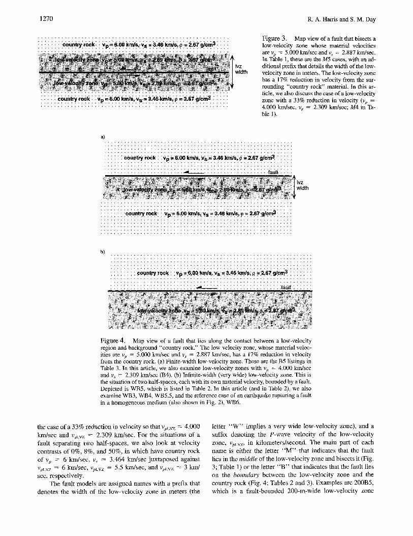
Table 1 Summary of Results--Fault-Bisected Low-Velocity Zones

LVZ Model LVZ v~v (right) Max. 4% Width (m) Name Location LVZ ve,v~ v~v (left) (kin/see) (bars)

100 100M5 middle 200 200M5 middle 400 400M5 middle 600 600M5 middle 800 800M5 middle

1000 1000M5 middle 1200 1200M5 middle 1400 1400M5 middle 1600 1600M5 middle 2000 2000M5 middle 3000 3000M5 middle 4000 4000M5 middle

100 100M4 middle 200 200M4 middle 400 400M4 middle 600 600M4 middle 800 800M4 middle

1000 1000M4 middle 1200 1200M4 middle 1400 1400M4 middle 1600 1600M4 middle 2000 2000M4 middle 3000 3000M4 middle 4000 4000M4 middle

5.0, 2.887 5.0, 2.887 5.0, 2.887 5.0, 2.887 5.0, 2.887 5.0, 2.887 5.0, 2.887 5.0. 2.887 5.0. 2.887 5.0. 2.887 5.0. 2.887 5.0. 2.887 4.0. 2.309 4.0. 2.309 4.0 2.309 4.0 2.309 4.0 2.309 4.0, 2.309 4.0, 2.309 4.0, 2.309 4.0, 2.309 4.0, 2.309 4.0, 2.309 4.0, 2.309

symmetry 3.05 0 " 3.05 0 " 3.0 0 " 3.0 0 " 4.8 0 " 4.4 0 " 4.5 0 " 4.0 0 " 2 .7 0

" 2 .7 0

" 2.7 0 " 2 .6 0

" 3.00 0 " 3 . 0 0 0

" 2.9 0 " 3.1" 0 " 3.8 0 " 3.8 0 " 3.8 0 " 3.8 0 " 3.8 0 " 3.8 0 " 2.1 0 " 2.1 0

*Propagates at 3.l km/sec, at 3.5 to 4 secs, dips down to Va.vz, then jumps up again to 3.1 km/sec.

Table 2 Summary of Results Wide Fault-Bounded Low-Velocity Zones

LVZ Model LVZ v~v (left) v~p (right) Max. Aa,, Width (m) Name Location LVZ vp,v s (km/sec) (kro/sec) (bars)

Infinite WB6 boundary 6.0, 3.464 3.10 3.10 0 Infinite WB5.5 boundary 5.5, 3.175 3.00 3.00 80 Infinite WB5 boundary 5.0, 2.887 2.80 2.85 210 Infinite WB4 boundary 4.0, 2.309 4.20 2.45 310 Infinite WB3 boundary 3.0, 1.732 3.10 2.10 300

Table 3 Summary of Results--Fault-Bounded Low-Velocity Zones

LVZ Model LVZ voa p (left) v~p (righ0 Max. Aan Width (m) Name Location LVZ vp,v~ (km/sec) (k_n'dsec) (bars)

200 200135 boundary 5.0, 2.887 3.10 3.10 90 400 400B5 boundary 5.0, 2.887 3.00 3.00 170 600 600B5 boundary 5.0, 2.887 3.00 3.20 310 800 800B5 boundary 5.0, 2.887 3.00 2.90 320

1000 1000B5 boundary 5.0, 2.887 2.90 2.90 330 200 200B4 boundary 4.0, 2.309 3.00 3.00 210 400 400B4 boundary 4.0, 2.309 4.40 2.80 270 600 600B4 boundary 4.0, 2.309 4.40 2.90 330 800 800B4 boundary 4.0, 2.309 4.20 2.70 350

1000 1000B4 boundary 4.0, 2.309 4.30 2.70 350


whose P-wave velocity is 5 km/sec, WB3, which is a fanlt- bounded very wide low-velocity zone whose P-wave velocity is 3 km/sec, and 4000M4, which is a 4000-m-wide fanlt- bisected (fault in the middle) low-velocity zone with VpLvz = 4 km/sec.

Rupture Velocity

The effects of a fault-bisected (M) low-velocity zone on a simulated earthquake's rupture velocity are summarized in Table 1. The rupture velocity is most sensitive to the widest fault-bisected low-velocity zones. In those situations, the rupture velocity is constrained by the elastic wave velocities of the low-velocity zone, and the terminal rupture velocity appears to approach the Rayleigh-wave velocity of the low- velocity zone, approximately 0.92 VsLvz. This is most obvi- ous for the 4-km-wide fanlt-bisected low-velocity zones (4000M). As the low-velocity zone narrows from 4 km width, the rupture velocity is little affected until between 1.5 and 2 km width when the rupture becomes supershear (faster than the shear-wave velocity of the country rock). This effect must be a result of interference between stresses concentrated at the crack tip and stress waves reflected back to the crack tip from the low-velocity zone/country-rock boundary, perhaps as converted phases. For widths of 600 m or less (600M to 100M), the rupture velocity is once again subshear, and as the low-velocity zone narrows, it is increasingly controlled by the elastic wave velocities of the country rock. As expected, in very narrow low-velocity zones, the terminal rupture velocity, just before the rupture has reached the end of the 27-km-long fault, approaches the Rayleigh-wave velocity of the country rock, irrespective of the LVZ velocities. Due to symmetry conditions across the fault, for all (fanlt- bisected) low-velocity zone widths, the rupture travels at the same velocity in the directions to the left and to the right of the simulated earthquake's nucleation zone.

The fault-bounded low-velocity zone cases exhibit some complex behavior. WB6 is our reference case of similar material on either side of the fault (Fig. 2). Due to the symmetry of this homogeneous model, the rupture velocities to the right and left of the nucleation zone are both 3,1 kin/ sec, or approximately the Rayleigh-wave velocity (Table 2). As the material velocity of the low-velocity zone decreases (WB5.5 to WB3) from that of the country rock, some inter- esting phenomena are observed. These phenomena are re- lated to two factors that become increasingly important as the seismic velocity contrast across the fault increases. The first factor is the ability of an unbonded fault to support a trapped interface wave under certain conditions, as discussed in the Appendix. The second factor is the development of normal stress perturbations across the fault during rupture.

As shown in the Appendix, an unbonded interface between dissimilar elastic media can only support a free interface wave when the seismic velocity contrast is not too great, in which case the interface wave velocity must lie between the Rayleigh-wave velocities of the two half-spaces, and below the S velocity of either. When the two half-spaces are

identical, the interface wave travels at their common Ray- leigh-wave velocity. As expected on theoretical grounds, the Rayleigh-wave velocity coincides with the terminal rupture velocity in this case, as we verified in simulation WB6. We would expect that, if the interface wave solution continues to exist when a velocity contrast is introduced across the fault, it would continue to control the rupture velocity. This expectation is verified by simulations WB5.5 and WB5. In both of these cases, conditions for existence of a trapped interface wave are met. Accordingly, the rupture velocities (3.0 km/sec for WB5.5, and 2.8 km/sec for WB5), in both directions, are nearly identical to the interface wave velocities for the respective cases, as derived analytically from equation (A8) in the Appendix (3.03 km/sec for WBS.5 and 2.84 km/sec for WB5).

For WB4 and WB3, conditions for the interface wave to exist are no longer met. As discussed in the Appendix and shown in Figure (A1), the interface wave exists only when the ratio of S-wave velocities (low-velocity half-space di- vided by high-velocity half-space) lies above a cutoff ratio. This cutoff depends on the density ratio and the Poisson's ratios, and for Poisson solids of equal density, the cutoff occurs at an S velocity ratio of 0.736. Thus, for a low-velocity zone S-wave velocity less than about 2.5 km/sec (P- wave velocity less than about 4.4 km/sec), we will be below the cutoff, and this is the case for both WB4 and WB3.

The result is that WB4 and WB3 show a departure from the pattern observed for the smaller material-velocity contrasts. In the absence of the singularity associated with the trapped interface wave, other stress concentrations must control the rupture velocity, and this is what is observed in the simulations. To the left of the nucleation point, for WB4 and WB3, rupture velocities are observed that are approximately equal to VpLvz. Furthermore, the rupture is now asymmetric, rupturing to the right at much slower rupture velocities.

This behavior can be understood by examining the simpler problem of slip induced by failure of a single-point asperity on a friction-free fault. The key element is the relationship between the normal stress and the slip velocity. Closed-form solutions can be obtained for these quantities as functions of time and position on the fault, and these are derived in the Appendix (equations A l l and A12). In the solution, slip pulses travel along the fault with the P and S velocities of the low-velocity zone and the country rock, respectively (Fig. 5). The slip-velocity function is symmetric about the nucleation point. When friction is present (as in WB4 and WB3), the rupture velocity would be expected to coincide, at least approximately, with the velocity of one of the strong slip pulses present in the frictionless solution, since these represent wave arrivals with strong shearing components on the fault plane. However, the analytic solution shows that the slip pulses are accompanied by perturbations to the normal stress on the fault, as shown in Figure 5. These normal stress changes are antisymmetric about the nucleation point. In the frictional case, the frictional strength is proportional to the fanlt-normal compressional stress.


20

P. S+S. S.S+ P. i

13-/13+ = s / ~

0 f -'q" ~ ~" - -~ - - slip velocity -20 . . . . normal stress

10

-10

~ _ / ~ + = 4 / 6

I¢ d I I

)

-1 P_S+ S_

- d

0 s. s+P. 1

Dimensionless Distance (X/o~+t)

Figure 5. A snapshot of the normalized slip velocity (pfl+XIA)Oa and normal stress (XIA)cr n for the case of asperity rupture on a friction-free fault, as given by equations (AI 1) and (A12). The cases shown are for equal-density Poisson solids. The upper curves are for a seismic velocity contrast of 5•6, analogous to numerical simulation WB5; the lower curves are for a velocity contrast of 4/6, analogous to simulation WB4. Arrows labeled P_+ and S_+ indicate the P and S arrivals associated with the two media. The large bold triangular arrows indicate the rupture velocities in the corresponding numerical simulations (which include friction). For the 5/6 velocity contrast, there is a trapped interface wave traveling slightly slower than S_, and this interface wave apparently controls rupture propagation in the numerical simulation as well. For the 4/6 velocity contrast, the interface wave no longer exists in the frictionless solution. The strongest slip pulses for which the normal stress change is tensional are S_ for propagation to the right (that is, in the direction of slip for the low-velocity half-space) and by P_ for propagation to the left, and rupture velocities for the numerical simulation are now controlled by these arrivals.

Therefore, rupture will be most likely to coincide with those wave arrivals that, in the friction-free problem, are associated with extensional perturbations to the normal stress. Conversely, rupture will be suppressed at those arrivals that are associated with compressional normal stress changes.

This is exactly what induces the asymmetric rupture in simulations WB4 and WB3. Since the normal stress is relatively compressional on the right side of the nucleation point where it lines up with the "VpLvz friction-free slip-velocity pulse," WB4 and WB3 cannot rupture at this speed to the right. Instead, they rupture at VsLVZ, at which speed a slip- velocity pulse lines up with relatively extensional normal

stress. To the left of the nucleation point, relatively extensional normal stress lines up with the "VpLvz slip-velocity pulse," so that WB4 and WB3 travel to the left of the nucleation point at VpLVZ. Therefore, the different travel speeds to the left and right of the nucleation point in WB4 and WB3 (Table 2) are explained by the interaction between the normal stress and the slip velocity. For comparison, Figure 5 also shows the analytic solution for the case corresponding to WB5. In that case, the dominance of the trapped interface wave is evident in the analytic solution and corresponds pre- cisely to the (symmetric) velocity of rupture seen in numerical solution WB5.

The effects of a fault-boundedfinite-width low-velocity zone on the rupture velocity are as follows (Table 3): To the right of the nucleation zone, for the finite-width low-velocity zone (200]3 to 1000B), rupture velocities are primarily dependent on the width of the low-velocity zone. Except for the case of 600 m width (600B), where the rupture velocity increases slightly (perhaps due to arrivals reflected from the material interface across the LVZ from the fault), the rupture velocity slows in accordance with the low-velocity zone width. Due to a lack of symmetry in the fault-bounded low- velocity zone models, the rupture velocities to the left and right of the nucleation zone are not necessarily the same. For the B5 cases (200B5 to 1000B5), where VpLvz = 5.0 kin/ sec, the rupture velocities to the left of the nucleation zone decrease overall as the low-velocity zone increases in width and are not drastically different from the rupture velocities in the opposite direction. This near symmetry of rupture when the velocity contrast is low is consistent with our ex- pectations based on the analysis of the infinite-width (very wide) low-velocity zone above. The difference between propagation in the directions to the right and left of the nucleation zone is more conspicuous for the B4 cases, where VpLvz = 4.0 km/sec, consistent again with the analysis based on normal stress changes. Whereas 600B4 to 1000B4 all travel to the right of the nucleation zone at maximum rupture velocities that are subshear relative to the country rock, to the left of the nucleation zone, the maximum rupture velocities are supershear relative to the country rock's material velocity. The behavior of B4 is best explained by a combi- nation of interference from reflected arrivals from the welded low-velocity zone/country rock interface and the sig- nificance of the antisymmetric normal stress (as in the WB4 case discussed previously).

Shape of the Slip Function

For our reference case (WB6), there is no low-velocity zone near the fault. As Figure 6 shows, slip continues behind the rupture front, with no healing after passage of the rupture. This is characteristic of propagating crack models in which the frictional strength drops at the time of rupture and does not subsequently recover strength during the slip process. Arrest of slip in such models occurs as a result of the confinement of slip on a surface of finite dimensions, and the duration of slip at a point is of order a/fl, where a is the


WB6 (Homogeneous)

10-

10

2.0 seconds

3.0 seconds

_L ._J o

.~>,1o

g

n-

-14 -12 -10 -8 -6 -4 -2 0 2 4 6 8 10 12 14

4.0 seconds

Along-fault distance from nucleation point (km)

Figure 6. Rupture of a fault in a homogeneous material with Vp = 6.0 km/sec (WB6) shows that dynamic crack models using a slip-weakening fracture criterion generally do not exhibit "Heaton slip pulse" (Heaton, 1990) behavior. Plots of relative velocity (rn/ sec) between the two sides of the fault at 2.0, 3.0, and 4.0 sec after nucleation. Much of the fault is slipping behind the rupture front, as shown by the long tail reaching back toward the nucleation point.

source dimension and fl the S-wave velocity. Heaton (1990) has demonstrated that slip in actual earthquakes apparently is of shorter duration than would be predicted from the dimensions of the earthquake rupture. The short rise times characteristically observed for earthquakes can be attributed to one of several phenomena, including velocity-dependent friction (e.g., Heaton, 1990) and secondary length scales associated with stress and/or strength heterogeneity on the fault (Mikumo and Miyatake, 1987; Beroza and Mikumo, 1996; Day et al., 1996).

In this article, we investigate the effect that material- velocity heterogeneity might have on the duration and shape of the slip velocity. The detailed results for the fault-bisected (M) low-velocity zone depend on the choice of low-velocity zone material velocity. In both cases (MS and M4), the addition of a finite-width low-velocity zone adds complexity

to the slip-velocity pulse and changes its shape from that depicted for the reference case, WB6 (Fig. 6). 400M5 (Fig. 7a) generates at least two phases, the first traveling near 0.9v . . . . . ~ ro~k, the second much smaller and traveling at V,Lvz. The greater velocity contrast present in 400M4 (Fig. 7b) leads to even more complex slip. An initial, narrow velocity pulse of about 1 km in width is followed by oscillatory behavior that is due to the interaction of the waves with the moderate-width (400-m) low-velocity zone. Slip is tempo- rarily arrested about 1 km (approximately 0.3 sec) behind the rupture front. However, slip reinitiates, and the total duration of slip is still controlled by the overall fault dimension.

The slip velocities generated by the fault-bounding low- velocity zone models also show variations from the reference case. WB5 shows a slip-velocity function (Fig. 8) on the right side of the nucleation zone that is similar to the reference case, WB6, except that the pulse is much narrower. On the left side of the nucleation zone, the same phase is smaller in amplitude and somewhat broader. These features can be qualitatively understood on the basis of the analysis of the frictionless case. WB5 is a case for which the trapped interface wave exists on the fricfionless interface. To the right of the nucleation point, the slip and normal stress are in phase; that is, positive slip is associated with extensional normal stress. Therefore, in the corresponding simulation with friction, the normal stress change enhances the dynamic shear stress drop to the right of the nucleation point, pro- ducing a large slip velocity. Conversely, to the left, positive slip is associated with compressional normal stress in the interface wave. Consequently, in the simulation with friction, slip velocity is lower at the rupture front, and the slip pulse, therefore, is more protracted. 400B4 and 400B5 (Figs. 9a and 9b), which are finite-width fault-bounded LVZs, show a very narrow initial pulse and, like the finite-width fault- bisected cases, additional pulses traveling at V~Lvz. In 400]34, the slip function to the right of nucleation is particularly complex, showing multiple phases of slipping and sticking. The width and velocity contrast in this simulation may be near or outside the extremes permitted by seismic observations of fault-zone-trapped waves (e.g., Li et aL, 1994a); however, if similar conditions are realized in fault zones, then this multiple sticking and slipping behavior might provide a mechanism to enhance the radiation of high-frequency seismic waves. Rupture in 400B4 is asymmetric, running faster to the left, as was the case for the infinite-width (very wide) low-velocity zone of the same velocity contrast. The relatively broad slip pulse behind the rupture front on the left (about 2 km behind the rupture front in the 4.0-sec frame) is the leaky mode pulse associated with the frictionless interface wave, which is no longer trapped but still shows up as a discernible arrival in the slip function.

While the presence of a low-velocity zone adds much complexity to the slip function in some cases, and sometimes results in brief episodes of sticking, it does not lead to short total duration of slip. Thus, by itself, the fault-zone low- velocity zone cannot explain observations of short slip du-


a) 400M5

10

10

5 ¸

0

£ .~>.10 o o >

.~ s

0

b) 400M4

2.0 seconds

3.0 seconds

L.----

4.0 seconds

-14-12-10 -8 -6 -4 -2 0 2 4 6 8 10 12 14


lO

0

g >,10 o o Q~

>

5 ._>

n-

o

2.0 seconds

3.0 seconds

4.0 seconds

-14-12-10 -8 -6 -4 -2 0 2 4 6 8 10 12 14


Figure 7. Relative velocity (m/sec) between the two sides of the fault at 2.0, 3.0, and 4.0 sec after nucleation for the case of a fault that bisects a finite-width (in this case, 400 m wide) low-velocity zone (Fig. 4). (a) For 400M5, the simulated earthquake does not exhibit Heaton slip-pulse behavior. (b) For 400M4, the relative velocity goes to zero behind the rupture front, then bounces up again, implying that the fault has not healed behind the rupture front.

ration in the context of a crack model with a conventional friction law. We must still invoke a self-healing constitutive law, stress and/or strength heterogeneity, or some other mechanism.

Normal Stress Reduction

For a planar fault embedded in a homogeneous medium, although the shear stress on the fault can vary from its initial value as a function of time, the normal stress across the fault remains constant as its initial value (e.g., 100M to 4000M in Table 1, where the material is the same on both sides of the fault). This condition of constant normal stress across a planar fault is not upheld when the material velocity changes across the fault, as it does for all of our fault-bounding cases, 200B to 1000B, and WB (except for WB6, which is the reference case with no velocity contrast). In these situations, the normal stress is coupled to the shear stress and slip on the fault.

Tables 2 and 3 show the largest normal stress reduction (i.e., reduction of the fanlt-normal compressive stress) that

we observe for each fault-bounding case, including the WB cases using a node spacing of 50 m. We present the numbers in the tables for qualitative comparison among the low-velocity zone cases but note that the absolute value of the normal stress reduction cannot be resolved by this type of numerical simulation and is dependent on the node spacing used in the finite-difference grid. We find that this dependence on numerical discretization persists down to 10-m node spacing, the smallest we investigated: Finer node spacings produce higher normal stress reduction, as originally noted by Andrews and Ben-Zion (1997). The largest reductions in normal stress along the fault all occur on the right side of the nucleation point, that is, where the slip direction on the low-velocity side of the fault is in the rupture propagation direction. This asymmetry leads to the amplitude of the slip velocity also being largest on the right side of the nucleation point. Where the normal stress reduction is largest, the amplitude of the relative slip velocity is also largest. This is apparent when comparing the results from the B4 and B5 cases (e.g., Figs. 9a and 9b showing 400B4 and 400B5), as noted earlier. The maximum normal stress re-


WB5

1 0

10

0

E ~0

o O H > ID 5 .>_

II1

0

2.0 seconds

3.0 seconds

4.0 seconds

-14-12-10 -8 -6 -4 -2 0 2 4 6 8 10 12 14


Figure 8. Relative velocity (m/sec) between the two sides of the fault at 2.0, 3.0, and 4.0 sec after nucleation for a fault that lies on the boundary between two half-spaces (WB5). Much of the fault is slipping behind the rupture so the simulated earthquake is not exhibiting Heaton slip-pulse behavior.

duction that we compute using 50-m node spacing is approximately 350 bars, for fault-bounded LVZs of 800 and 1000 m width (800B4 and 1000B4). Since the initial values of the normal stress and stress drop are 2000 and 75 bars, respectively, for all of our simulations, 350 bars, which is approximately 4.7 times the stress drop, represents a stress reduction of 17.5%. When the grid size is reduced to 25 m, the normal stress reduction is nearly doubled, and it nearly doubles again for 10-m gridding. Andrews and Ben-Zion (1997) have shown that this mechanism can even lead to reduction of the normal stresses to zero in the vicinity of the crack tip.

Discussion

As shown above, the presence of a low-velocity zone can significantly modify the rupture velocities, slip-velocity functions, and normal stresses predicted by simple earth-

quake models. In this section, we discuss how these results impact our current understanding of the earthquake process.

The rupture velocities of the simulated earthquakes are modified by the presence of a low-velocity zone, in accordance with wave theory. Li and Vidale (1996) used 2D simulations of a point source in the vicinity of a narrow (200 m wide) low-velocity zone. They showed that there are many waveforrns to analyze even without including the rupture process of the earthquake. Therefore, when incorporating the rupture process into the low-velocity zone problem, as we do, interface waves and reflected and refracted arrivals com- bine to create a picture that is much more complex than that of a simple spontaneous rupture in a uniform half-space (case WB6).

In situations where the low-velocity zone is bisected by the fault, the rupture velocity is increasingly slowed by the low-velocity zone as the zone widens. At the narrowest LVZ widths resolvable by our simulations, 100 to 200 m, which are also the widths obtained by Li et al. (1994a, b), for the regions around the 1992 M7.3 Landers, California, earthquake, the rupture velocity is decreased by approximately 3% from a simulated earthquake in a homogeneous medium, a change that is too small to have any seismically observable consequences. If the fault-bisected low-velocity zone is much wider, say on the order of 2 to 4 km (e.g., Cormier and Spudich, 1984), then the reduction in the rupture velocity would be more than 10%. The low-velocity zone can also induce asymmetry in rupture velocity through its effect on the normal stress. Andrews and Ben-Zion (1997) have shown that, for the special case in which the static and dynamic friction coefficients are equal, purely unilateral rupture can be initiated and sustained. We have identified another form of rupture asymmetry that is likely to be most significant when the seismic S velocity ratio falls below a critical value controlling the existence of a Rayleigh-like interface wave. Analysis of waves on a frictionless interface gives a value of approximately 0.74 for the critical S-wave velocity ratio (for Poisson solids, and a density ratio of 1). The simulations with the slip-weakening friction law con- firm that significant rupture asymmetry develops when the velocity ratio falls below this threshold.

The low-velocity zone acts to modify the slip function from that predicted for a crack model in a uniform material. Although the case of VpLVZ = 4.0 krn/sec does look significantly different from that of a uniform medium, the overall duration of the slip function is not reduced. Even though the initial part of the slip pulse is narrower for this case than for the reference case, and slip becomes oscillatory, in no situation do we observe early cessation of slip. This implies that another factor, such as velocity-dependent friction or strength heterogeneity, must be invoked to explain the short slip durations inferred for earthquakes.

We examined the effects of a low-velocity zone on the normal stress, in an attempt to see if material-velocity contrasts across faults could help explain the lack of a heat-flow anomaly across some of California's faults (Henyey, 1968;


a) 400B4

lO

2.0 seconds

0

>,10 o o O) > .~ 5

or

b) 4 0 0 B 5

3.0 seconds

4,0 seconds

0 -- ~ ----7--.-.-- -14-12-10 -8 -6 -4 -2 0 2 4 6 8 10 12 14


10

0

v

O

> ill 5

=-

IT 0

2.0 seconds

3.0 seconds

4.0 seconds

1

- t 4 - 1 2 - 1 0 -8 -6 -4 -2 0 2 4 6 8 10 12 14


Figure 9. Relative velocity (m/sec) between the two sides of the fault at 2.0, 3.0, and 4.0 sec after nucleation for finite-width (in this case, 400 m wide) fault-bounded LVZs. (a) 400B4 is very "ringy," showing the influence of the LVZ on the waveforms. (b) 400B5 is a simpler picture than 400B4, but still shows a second arrival that is due to the presence of the finite-width low-velocity zone (compare with Fig. 8).

Brune et al., 1969; Lachenbrnch and Sass, 1980) by significantly reducing the normal stresses during sliding and, therefore, the frictional heat generation. Similar to the results of Andrews and Ben-Zion (1997), we find that a velocity contrast reduces the normal stress, but it has so far not been possible for us to accurately assess the magnitude of this reduction. Node spacings of 50 m in the simulations produce a reduction on the order of 20% near the crack tip, whereas finer node spacings produce higher reductions. The largest normal stress reductions, and the evidence of grid-size dependence in the calculations, are both strongly concentrated very near the crack tip. It remains an open question whether normal stress reduction by this or a similar mechanism can occur on a scale sufficient to significantly lower the frictional heat generation on faults.

A c k n o w l e d g m e n t s

Thanks to Jim Rice for stimulating discussion and to Yehuda Ben-Zion and Joe Andrews for conversations early in the course of this work. Jack Boatwright, Nick Beeler, Michel Campillo, and Greg Beroza provided thoughtful reviews. This work was partially supported by an NSF VPW

fellowship to RAH at Stanford University during 1994 and 1995 and by grants to SMD and RAH from the Southern California Earthquake Center. This is SCEC Contribution Number 348.

References

Aki, K. and P. G. Richards (•980). Quantitative Seismology, Theory and Methods, W. H. Freeman and Co., New York.

Andrews, D. J. (1976a). Rupture propagation with finite stress in antiplane strain, J. Geophys. Res. 81, 3575-3582.

Andrews, D. J. (1976b). Rupture velocity of plane strain shear cracks, J. Geophys. Res. 81, 5679-5687.

Andrews, D. J. and Y. Ben-Zion (1997). Wrinkle-like slip pulse on a fault between different materials, Z Geophys. Res. 102, 553-571.

Ben-Zion, Y., S. Katz, and P. Leary (1992). Joint inversion of fault zone head waves and direct P arrivals for crustal structure near major faults, J. Geophys. Res. 97, 1943-1951.

Beroza, G. C. and T. Mikumo (1996). Short slip duration in dynamic rupture in the presence of heterogeneous fault properties, J. Geophys. Res. 101, 22449-22460.

Brune, J. N., T. L. Henyey, and R. F. Fox (1969). Heat flow, stress, and rate of slip along the San Andreas fault, California, J. Geophys. Res. 74, 3821-3827.

Campillo, M. and R. J. Archuleta (1993). A rupture model for the 28 June


1992 Landers, California, earthquake, Geophys. Res. Lett. 20, 647- 650.

Cormier, V. F. and P. Spudich (1984). Amplification of ground motion and waveform complexity in fault zones: examples from the San Andreas and Calaveras faults, Geophys. J. R. Astr. Soc. 79, 135-152.

Day, S. M. (1982a). Three-dimensional finite difference simulation of fault dynamics: rectangular faults with fixed rupture velocity, Bull. Seism. Soc. Am. 72, 705-727.

Day, S. M. (1982b). Three-dimensional simulation of spontaneous rupture: the effect of nonuniform prestress, Bull. Seism. Soc. Am. 72, 1881- 1902.

Day, S. M., G. Yu, and R. A. Harris (1996). Modeling the dynamics of complex fault zones, EOS 77, F48-F49.

Harris, R. A. and S. M. Day (1993), Dynamics of fault interaction: parallel strike-slip faults, J. Geophys. Res. 98, 4461-4472.

Harris, R. A., R. J. Archuleta, and S. M. Day (1991). Fault steps and the dynamic rupture process: 2-d numerical simulations of a spontaneously propagating shear fracture, Geophys. Res. Lett. 18, 893-896.

• Heaton, T. H. (1990). Evidence for and implications of self-healing pulses of slip in earthquake rupture, Phys. Earth Planet. Interiors 64, 1-20.

Henyey, T. L. (1968). Heat flow near major strike-slip faults in California, Ph.D. Thesis, California Institute of Technology, Pasadena, Califor- nia.

Hough, S. E., Y. Ben-Zion, and P. Leary (1994). Fault-zone waves observed at the southern Joshua Tree earthquake rupture zone, Bull. Seism. Soc. Am. 84, 761-767.

Ida, Y. (1972). Cohesive force across the tip of a longitudinal shear crack and Griffith's specific surface energy, J. Geophys. Res. 84, 3796- 3805.

Lachenbruch, A. H. and J. H. Sass (1980). Heat flow and energetics of the San Andreas fault zone, J. Geophys. Res. 85, 6185-6223.

Lees, J. M. (1990). Tomographic P-wave velocity images of the Loma Prieta earthquake asperity, Geophys. Res. Lett. 17, 1433-1436.

Less, J. M. and P. E. Malin (1990). Tomographic images of P-wave velocity variation at Parkfield, California, J. Geophys. Res. 95, 21793-21804.

Li, Y.-G. and J. E. Vidale (1996). Low-velocity fanlt-zone guided waves: numerical investigations of trapping efficiency, Bull. Seism. Soc. Am. 86, 371-378.

Li, Y.-G., P. Leafy, K. Aki, and P. Malin (1990). Seismic trapped modes in the Oroville and San Andreas fault zones, Science 249, 763-766.

Li, Y.-G., K. Aki, D. Adams, A. Hasemi, and W. H. K. Lee (1994a). Seis- mic guided waves trapped in the fault zone of the Landers, California, earthquake of 1992, J. Geophys. Res. 99, 11705-11722.

Li, Y.-G., J. E. Vidale, K. AM, C. J. Marone, and W. H. K. Lee (1994b). Fine structure of the Landers fault zone: segmentation and the rupture process, Science 265, 367-370.

Li, Y.-G., F. L. Vernon, and A. Edelman (1995). The fine structure of the San Jacinto fault near Anza, California inferred by fault-zone trapped waves, EOS 76, 398.

Madariaga, R. (1976). Dynamics of an expanding circular fault, Bull. Seism. Soc. Am. 66, 639-666.

Magistrale, H. and C. Sanders (1995). P-wave image of the Peninsular Ranges batholith, southern California, Geophys. Res. Lett. 22, 2549- 2552.

Michael, A. J. mad D. Eberhart-Phillips (1991). Relations among fault behavior, subsurface geology, and three-dimensional velocity models, Science 253, 651-654.

Mikumo, T. and T. Miyatake (1987). Numerical modeling of realistic fault rupture processes, in Seismic Strong Motion Synthetics, B. Bolt (Ed- itor), Academic, New York, 91-151.

Nicholson, C. and J. M. Lees (1992). Travel-time tomography in the north- eru Coachella Valley using aftershocks of the 1986 ML 5.9 North Palm Springs earthquake, Geophys. Res. Lett. 19, 1-4.

Okubo, P. G. and J. H. Dieterich (1986). State variable fault constitutive relations for dynamic slip, in Earthquake Source Mechanics', S. Das, C. Scholz, and J. Boatwright (Editors), American Geophysical Mono- graph 37, 25-35.

Rice, J. R. (1980). The Mechanics of earthquake rupture, in Phys. Earth's Int. (Proc. of the Int. School of Physics Enrico Fermi, Course 78,

1979), A. M. Dziewonski and E. Boschi (Editors), Italian Phys. Soc., North-Holland, Amsterdam, 555~549.

Wald, D. J. and T. H. Heaton (1994). Spatial and temporal distribution of slip for the 1992 Landers, California earthquake, Bull. Seism. Soc. Am. 84, 668-691.

Weertman, J. (1963). Dislocations moving unifolmly on the interface between isotropic media of different elastic properties, J. Mech. Phys. Solids 11, 197-204.

Zhao, D. and H. Kanamori (1992). P-wave image of the crust and upper- most mantle in southern California, Geophys. Res. Lett. 19, 2329- 2332.

Appendix Asperi ty Failure on Frictionless Interface

To capture some insight into the velocities of rupture to be expected along an interface between contrasting elastic half-spaces, we consider the following idealization. Let the uniform, isotropic, elastic half-spaces z < 0 and z > 0 have contrasting material properties. Their densities, P velocities, and S velocities will be denoted by p, c~, and r , respectively, with subscripts - and + . We impose interface conditions requiring continuity of the normal component of displacement across the interface at z = 0. The interface is frictionless, tangential slippage being permitted across it, except on an asperity consisting of an infinitely long strip of width L about the y axis, on which the tangential component of displacement is continuous for time t < 0. Forces are applied at infinity to bring the tangential stress on this infinite strip to the level A/L, where L is the width of the strip in the x direction. Then we take the limit L --~ 0, in which case the tangential stress is nonzero only along a line asperity on the y axis, where its value is Ac~(x).

At t = 0, the asperity is assumed to rupture, the tangential stress dropping instantaneously to zero. Then the dis- turbances in the displacement and stress components (relative to their equilibrium values), ui and aij, are independent of the y coordinate and satisfy the equations of elastodyn- amics with boundary conditions

u z (x,0-,t) = u z (x,0+,t),

% (x,0-,t) = ~zz (x,0+,t),

~xz (x,O-,t) = ~xz (x, O+,t) = - A r ( x ) H ( t ) .

(A1)

After Laplace transformation on time and Fourier transformation on x, taking into account radiation conditions, and making the substitution k = isp, the solution for displacement and stress components takes the form

Ux = pP+_e T-s~+-z + #l+S+ e;s~+-z,

iu~ = + i ~ ± P + e -vs~±z + pS+_e =s~+J,

s - l a ~ = p±(2fl2±p 2 - 1)P±eXS~-*_z

+__ 2ip ±f l~q +pS +e ~s~+-z,

- i s - Jaxz = +- 2 i p ± f l ~ ± p P ± e ~¢+-z

+ p ± ( 2 f l 2 p 2 - 1)S±e~"+-z,

(A2)


where

~± = (Ot_~2 __ p2)1/2 Im(~+) > 0,

tl ± = (fl_~2 _ p2)1/2 Re(q_+) > 0. (A3)

The wave amplitudes P__+ and S + are determined by the boundary conditions (A1), which upon transformation yield

- i ~ _ p - i ~ +

p _ ( 2 f l Z p 2 - 1) -2 ip_ f l2_~l_p - -p+(2~2+p 2 - 1)

- -2 ip_f l2_~_p p_(2flZ__p z - 1) 0 0 0 2ip+fl2+~+p

A{ o. o,s) = -

qGfp)[(1 - r) _fp) +

(A9)

A homogeneous solution to (A5) exists when the deter- minant appearing in the denominator of (A8) and (A9)

- 2ip+flZ+tl+p S_ 0 P+

p+(2fle+p 2 - 1) S+ = - 7 .

(A4)

Eliminating P + from the system, via substitution from rows 3 and 4, yields

[ ra -raV ]fS_]=-iA[ 1 - r ] + '

where r /z _/kt +, y ± 2p 2 - 2 = = - t ± , and 'R±(p) are the respective Rayleigh functions for the half-spaces z > 0 and z < 0 ,

qC+(p) = 4p:¢_+e± + G . (A6)

The solution to (A5) is

iA {(1 - r-~)¢_~+(p) + /~;2 [¢+7- + ¢-7+1~ S_ = s:/--- ] /~_-:¢_R+(p) + r/~7~f+R_fp) J'

iA {(1 - r)~+'R_(p) + ,622 [¢+7- + ¢-7+11 S+ -- s2fl+ fl__2¢ CR+(p ) + rfl+2~+,R_(p) j.

(A7)

Then, from (A2), we get the following solution for the (doubly transformed) displacement discontinuity

& x =- ux (p,z,S)lz=O+ - Ux(p,z,S)lz=O-,

AI (÷ +) &x(p,s) = 2t~ +s z - +

(7- + 2,/_~_)[(1 - r-~)R+(p) + fl+2(~z~+y_ + ?+)l +

+

/L-2~_R+(p) + rp ;2G~_(p)

(7+ + 2q+~+)[(1 - r)~R (p) + fiz z (7- + ~+1~-7+)].].

J (A8)

Similarly, the solution for the normal stress on the fault, an =-- azz(p,z,s)lz= o is

(A5)

equals zero, in which case (A8) and (A9) each have a simple pole. We will take t _ to be the lower of the 2 S velocities. If a denominator zero exists for p real and p > fl_-x, the corresponding homogeneous solution represents a propagating disturbance trapped at the interface. Weertman (1963) describes conditions for the existence of this interface wave. From the properties of R_+(p) (it is positive in the limit of large p and has a single real zero fo rp > fiT_ 1), it is easy to see that, if the interface wave exists, the corresponding value of p must lie between the two half-space Rayleigh-wave slownesses. As the contrast in half-space S-wave velocities increases (for some fixed values of the Poissons ratios and density ratio), the pole migrates along the real axis toward the branch point a tp = fl-_ ~. Further increase in the velocity contrast moves the pole through the branch cut and off the real p axis onto a lower Riemann sheet, at which point the interface wave no longer exists. Figure AI shows the cutoff S velocity ratio, as a function of the S-to-P ratios. In the limit of very low S-to-P ratios in both half-spaces, and equal densities, the cutoff S velocity ratio approaches (1 - X~o) 1/2, where Xo is the real root of x 4 - 4x + 2, or a velocity ratio of about 0.839.

The forms of (A8) and (A9) are such that we can invert the double transform via the Cagniard-de Hoop method (Aid and Richards, 1980, p. 224). As usual, the inverse Fourier integrals are manipulated into the form

ice

c~u x (x,s) = 2s Im f ~u(p,s)e-WXdp 0

(A10)

and a similar equation for an. Finally, we deform the inte- gration contour onto the positive real axis. In the event the integrand has a pole on the upper Riemann sheet, it will lie on the real axis. In that case, we take the principal value of


0.8

0

Q- 0.75

+ CO.

0.7

0.65

0,25 i ' i ' i . . . . . . . 0 3 0.35 0 4 0.45 0 5 0.55 0.6 0,65 0.7

~-/a-

Figure A1. As the contrast in half-space S-wave velocities increases (for some fixed values of the Pois- sons ratios and density ratio), the pole migrates along the real axis toward the branch point at p = fl-1. Further increase in the velocity contrast moves the pole through the branch cut and off the real p axis onto a lower Riemann sheet, at which point the interface wave no longer exists. This figure shows the cutoff S velocity ratio, as a function of the S-to-P ratios. In the limit of very low S-to-P ratios in both half- spaces, and equal densities, the cutoff S velocity ratio approaches (1 - ~)v2, where x 0 is the real root of x 4 - 4x + 2, or a velocity ratio of about 0.839. For the cases that we investigate in this article, the S-to- P ratios for both materials are 0.577 (Poisson solid), and the density ratio is 1. Therefore, the interface wave can only exist for S-wave ratios above 0.736 (e.g., for cases WB5 and WB5.5).

the integral; the residue is purely real, so it makes no contribution to (A10) and can be ignored. With the change of

variables p = t/x, (A10) assumes the form of a Laplace transform, and we can identify the coefficient of e - s t in the

integrand as the transient slip function 6ux(x, t) . Taking into account the time differentiation implied by multiplication by s, the resulting slip velocity function is given by

6u(x,t) = A.. Im - + x#+

(7- + 2~_~_)[(1 - r-])cR+(p) q- fl+2(~_-1~+)2_ q- 7+)1 + B U ~ _ R + ( p ) + r B + 2 ~ + ~ _ ( p )

(7+ + 2~/+~+)[(1 - r )R_(p) + fl22(7_ + ~+1~_7+)].]

( A l l )

The corresponding result for the fault plane normal stress is

~r~ (x,t) = - I m - t

- + B : 2 ( y_ +

U.S. Geological Survey Mail Stop 977 345 Middlefield Road Menlo Park, California 94025

(R.A.H.)

Department of Geological Sciences San Diego State University San Diego, California 92182

(S.M.D.)

Manuscript received 23 December 1996.

(A12)

Effects of a Low-Velocity Zone on a Dynamic Rupture

Documents