Effect of Formation Size on Flocking Formation Performance ...

��

Citation: AlMuhaideb, S.; Touir, A.;

Alshraihi, R.; Altwaijry, N.; Qasem, S.

Effect of Formation Size on Flocking

Formation Performance for the Goal

Reach Problem. Appl. Sci. 2022, 12,

3630. https://doi.org/10.3390/

app12073630

Academic Editor: Kerstin Thurow

Received: 22 February 2022

Accepted: 31 March 2022

Published: 3 April 2022

Publisher’s Note: MDPI stays neutral

with regard to jurisdictional claims in

published maps and institutional affil-

iations.

Copyright: © 2022 by the authors.

Licensee MDPI, Basel, Switzerland.

This article is an open access article

distributed under the terms and

conditions of the Creative Commons

Attribution (CC BY) license (https://

creativecommons.org/licenses/by/

4.0/).

applied sciences

Article

Effect of Formation Size on Flocking Formation Performance forthe Goal Reach Problem

Sarab AlMuhaideb 1,* , Ameur Touir 1 , Reem Alshraihi 1, Najwa Altwaijry 1 and Safwan Qasem 2

1 Department of Computer Science, College of Computer and Information Sciences, King Saud University,Riyadh 11362, Saudi Arabia; [email protected] (A.T.); [email protected] (R.A.);[email protected] (N.A.)

2 Computer Engineering Department, Al Yamamah University, Riyadh 11512, Saudi Arabia;[email protected]

* Correspondence: [email protected]; Tel.: +966-11-805-2836

Abstract: Flocking is one of the swarm tasks inspired by animal behavior. A flock involves multipleagents aiming to achieve a goal while maintaining certain characteristics of their formation. Innature, flocks vary in size. Although several studies have focused on the flock controller itself, lessresearch has focused on how the flock size affects flock formation and performance. In this study,we address this problem and develop a simple flock controller for goal-zone-reaching tasks. Thedeveloped controller is intended for a two-dimensional environment and can handle obstacles aswell as integrate an additional invented feature, called sensing power, in order to simulate the naturaldynamics of migratory birds. This controller is simulated using the NetLogo simulation tool. Severalexperiments were conducted with and without obstacles, accompanied by changes in the flock size.The simulation results demonstrate that the flock controller is able to successfully deliver the flock tothe goal zone. In addition, changes in the flock size affect multiple metrics, such as the time requiredto reach the goal (and, consequently, the time required to complete the flocking task), as well as thenumber of collisions that occur.

Keywords: swarm; formation control; goal reach problem; simulation; flocking agents; sensingpower; flocking rules

1. Introduction

Many researchers have focused on robotic swarms—robot groups that co-operateto achieve a global goal in a complex environment [1]. The flocking problem, inspiredby the behavior of animals (e.g., birds flocking or fish schooling), is a subfield of swarmrobotics [2]. A swarm consists of a set of similar members having the same characteristicsand progressing in an asynchronous manner. There is no leader in the swarm directing othermembers to perform the planned tasks. Thus, a swarm operates in a decentralized context,where complex behavior arises through the labor of autonomous agents that are actingon local information. An agent cannot conclude the swarm aims without collaboratingwith the rest of the group [3]. One of the main components of a swarming system is theexhibition of cooperative behavior. A flock involves multiple agents that possess real-timegroup behavior capabilities that facilitate achieving a common target, such as foraging ormigration [4,5]. The design of swarm robotics systems is guided by swarm intelligenceprinciples. Brambilla [6] divided the swarm behaviors into four major categories—spatialorganization, navigation, decision making, and miscellaneous—each of which has differentareas of application. Schranz [7] proposed an extension to the categorization of the basicswarm behaviors. They used this taxonomy to classify a number of existing swarm roboticapplications from research and industrial domains. Several studies were orientated towardsmodeling swarm robots to increase the understanding of natural swarm systems [8]. In arobotic swarm, the collective behavior results from local interactions among the robots andbetween the robots and the environment. One area that researchers have investigated is

Appl. Sci. 2022, 12, 3630. https://doi.org/10.3390/app12073630 https://www.mdpi.com/journal/applsci

https://doi.org/10.3390/app12073630


https://creativecommons.org/

https://creativecommons.org/licenses/by/4.0/

https://creativecommons.org/licenses/by/4.0/

https://www.mdpi.com/journal/applsci

https://www.mdpi.com

https://orcid.org/0000-0002-2642-072X

https://orcid.org/0000-0002-5145-6484

https://orcid.org/0000-0002-7386-1886

https://orcid.org/0000-0003-0727-7494


https://www.mdpi.com/journal/applsci

https://www.mdpi.com/article/10.3390/app12073630?type=check_update&version=2

Appl. Sci. 2022, 12, 3630 2 of 29

the study of the efficiency in self-regulation of swarms of birds, schools of fish, and socialinsect colonies, whereas others initiated models to generate and optimize artificial swarmsystems as engineered in the field of swarm robotics [9]. One can notice the importanceof models that suggest novel empirical experiments, as well as the prominence of empiricexperimentation that results in relevant model parameterizations [10]. Dias et al. [8]published an extensive review presenting a discourse on a large panoply of features,covering swarm robotics.

The individual elements in such flocks move, while maintaining specific velocitiesand distances among each other without splitting. Reynolds [11,12] has specified threefundamental flocking rules: collision avoidance, flock centering, and velocity matching(alignment). Animal groups change their structure depending on internal or externalstimuli, thus maximizing the fitness of individuals as circumstances change [13]. Thebehavior of these agents, integrated within the structural order, results in changes ofdirection and shape without affecting the group’s coherence [13].

Formation control aims to produce control commands that are sufficient to drivemultiple agents to reach their status constraints [4]. To endow self-organization systemswith flexibility and robustness, controllers use decentralized mechanisms [14]. A controlleris an essential structure that is used in the implementation and simulation of swarmsystems [15]. There are three main approaches to formation control systems [4,12,16]:the leader–follower approach [12,17–19], the virtual structure approach [1,20,21], and thebehavior-based approach [5,14,16,22–26]. Despite the simplicity of the leader–followerapproach, it may suffer from being highly dependent on the leader agent and fromthe large amount of information exchange required between the leader and each of thefollowers due to being a centralized system [4]. Moreover, virtual structure approacheslack formation modification when the formation changes due to structural redesign, whichincreases the required computation and degrades collision avoidance abilities. On the otherhand, the behavior-based approach allows for the handling of multiple tasks using a singlecontroller [4]. Notably, in the literature, most researchers have used the behavior approach,due to the fact that the flocking task is usually directly inspired by natural animal behavior.

The flock size is the number of individuals within the flock. In nature, animalstend to have higher survival rates when being part of a group. In fact, group size isone of the primary defense mechanisms that animals adopt in order to limit predationrisks [27,28]. The size of a flock in nature can range from one species to hundreds ofdifferent species. Accordingly, flocking applications use different flock sizes, based onthe application objectives [29]. As the flock size increases, the rate of successful attacksdecreases [30]. Nevertheless, there are several disadvantages to grouping [30], includinggreater competition between group members and greater exposure to predators. On theother hand, some of the advantages of grouping are foraging, defense, alertness, and riskreduction [27,31].

Indeed, flock size is one of the main behavioral mechanisms used by animals tomanage their vulnerability to predation. Hintz et al. [32] studied the direct effect of flocksize on foraging success with respect to the predation risk. Cresswell [30] investigated howthe flock size risk thresholds differ for attack rate, success rate, or dilution. The optimal flocksize reflects a dynamic interplay between a diverse range of costs (competition, visibility,etc.) and benefits (defense, vigilance, etc.) associated with joining a group [27].

Most research has focused on constructing new methods or enhancing existing meth-ods related to flock formation and control. Consequently, fewer efforts have been madein studying the effects of flocking parameters, such as flock size, on the performance ofthe developed systems. Zhang et al. [26] have studied the impact of changing flock sizeon reaching the goal in a specific time. They conducted two types of experiments; thefirst one was applied to test their work, with the objective of reaching the goal in a fixedtime. For this experiment, they used 30 robots, and found that the flock could convergewithin a specific time. The second experiment focused on showing the effect of convergingtime when the flock size changed, with experiments using 2, 4, 6, . . . , 40 robots. They con-

Appl. Sci. 2022, 12, 3630 3 of 29

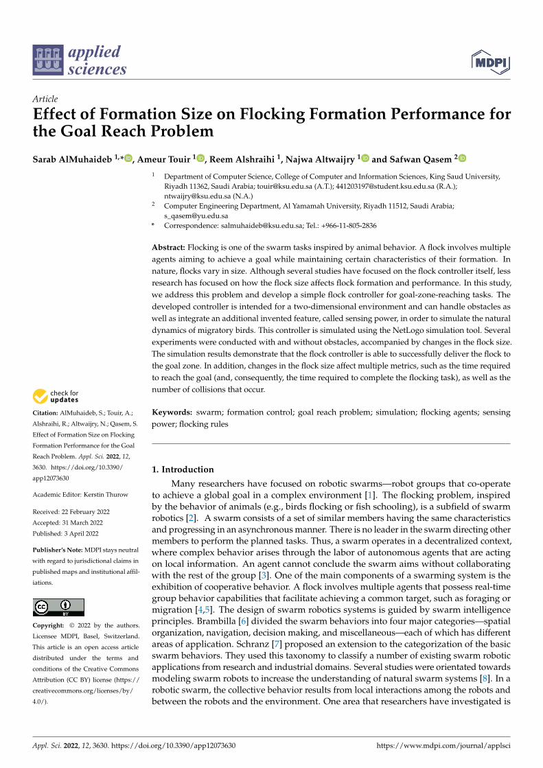
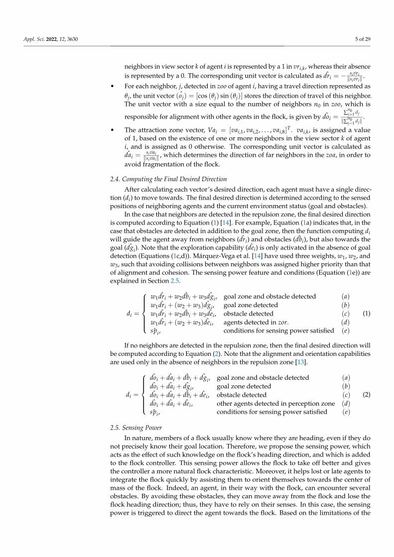
cluded that the convergence time decreases as the number of agents increases. Moreover,Márquez et al. [14] have used three types of experiments to test (i) the cooperative behavior,(ii) the optimized control parameters, and (iii) the objective functions, when using 5, 10,or 20 agents. They found that the number of agents and the existence of obstacles did notaffect the flock’s performance. Moreover, the performance of the flock was improved whenthe repulsion zone was small, and the orientation and attraction zones were large. Figure 1depicts these three different zones. The flock direction in the proposed work was decidedin consensus between the different agents. Therefore, they found that the complexity of thedetermined direction increases as the flock size increases. The importance of the orientationradius also increased as the flock size increased. On the other hand, Olfati [23] has proposeddifferent algorithms to simulate and study the flock behavior, according to their numberand distribution in free space and with obstacles. However, these works did not study howthe flock size affects the formation, whether the flock size affects the time it takes to reachthe goal, whether all agents successfully reach the goal, how much time the flock takes tomatch the velocity, and whether the flock maintains the flocking roles while exploring.

(a) (b)

Figure 1. Sensing zones and view sectors of agents: (a) The three agent perception zones; and (b) theeight view sectors.

In this paper, we study the relationship between flock size and its effect on the flockingsystem’s formation and performance. Inspired by previous works [13,14,16], a flockingsystem is constructed. Performance is measured according to a number of factors, includingthe flexibility towards reaching the goal (e.g., the time to reach the goal zone, number ofagents within the goal area), time to match the velocity, the number of applied flockingrules (e.g., separation, cohesion, and alignment), and the number of collisions that occur.Additional parameters are taken into account, such as the average distance to the center ofmass, goal localization time, and localization window.

2. Materials and Methods

The objective of this study is to evaluate the performance of a flock during a flockingtask with an unknown target zone. The tasks tackled in this paper are similar to those inthe studies [13,14,16]. However, this study is characterized by the objective functions itdefines, along with the various metrics used to analyze and evaluate the performance andbehavior of the controller.

2.1. Assumptions

The controller developed in this paper is based on an existing controller [14]. Somefeatures are used, such as the repulsion zone, attraction zone, orientation zone, and theview sectors of the agent, while others are added, such as the sensing power to replicate themigration of birds in nature. Completion of the task is determined when all agents reach

Appl. Sci. 2022, 12, 3630 4 of 29

the goal zone. First, some assumptions about the controller need to be highlighted—theseassumptions also represent the controller’s boundaries.

• The system is deployed in a two-dimensional geographical region;• Obstacles in the environment are static obstacles;• The arena size always fits the agents. It includes the initial zone and the goal zone;• The environment has a static goal located within the goal zone, which is a circular

region with a center, (gx, gy), and a radius, rg;• The initial zone is a circular region with a radius, rz;• Agents are homogeneous;• The positions of the agents are randomly generated within the initial zone;• The velocity of each agent is initially random, within a bounded range, (vmin, vmax);• The direction of each agent is initialized randomly;• Each agent can sense its neighbors within a maximum distance with radius ∆a, as

shown in Figure 1, from its position;• There exists a sensing power, which works as a hint towards the goal position (see

Section 2.5).

2.2. Flock Design and Representation

The proposed flock controller’s design is inspired by previous studies [13,14], whereeach agent is able to sense other neighbors and obstacles within three zones: the zone ofrepulsion, zor, with width ∆r; the zone of orientation, zoo, with width ∆o; and the zone of at-traction, zoa, with width ∆a (see Figure 1a). Each agent has several view sectors (in this case,eight sectors), Si = [u1, u2, . . . , u8]

T , where uk = [cos ((2k− 1)× π8 ) sin ((2k− 1)× π

8 )], asshown in Figure 1b. These view sectors are used to locate an agent within (0, 2π) radii.Agents then behave depending on the surrounding environment and their neighbors.

2.3. Behavior of Agents

Each agent behaves based on its surrounding environment and neighbors within theperception zones. Each agent, i, has a number of vectors that help to determine its direction.These vectors are as follows:

• A goal-zone-detection vector, Vgi = [vgi,1, vgi,2, . . . , vgi,8]T , where each vgi,k is equal

to 1 if a goal is detected in view sector k of agent i, within its perception area (zoa), andis equal to zero otherwise. The unit vector dgi, which denotes the desired direction ofagent i based on the goal detected, is calculated as follows: dgi =

si vgi‖si vgi‖

.

• An obstacle-detection vector, Vbi = [vbi,1, vbi,2, . . . , vbi,8]T , where each vbi,k is equal to

1 if an obstacle is detected in view sector k of agent i within its perception area, andis equal to zero otherwise. The unit vector dbi, which denotes the desired directionof agent i based on the opposite net direction of obstacles detected, is calculated as

follows: dbi = − si vbi‖si vbi‖

.

• An arena-exploration unit vector, ˆdei = [cos (θrand,i) sin (θrand,i)], is required, in orderto help the agent explore the unknown environment. This vector has a single value:a random angle in the range θrand,i ∈ (0, 2π). In the case where an obstacle has beendetected, the angle is modified to θrand,i ∈ (0, π), such that the agent heads towards aregion in the opposite direction of the observed obstacle.

On the other hand, agents also have to consider their neighbors, in order to avoidcollisions with each other, as well as maintaining the coherence of the flock, to avoidfragmentation, and to keep the agents aligned. Therefore, agents have another three vectorsdefining how they behave, according to their nearby neighbors. These vectors are definedaccording to the three zones (zor, zoo, and zoa) for each agent i, as follows:

• A repulsion zone vector Vri = [vri,1, vri,2, . . . , vri,8]T . This vector allows for the de-

tection of neighbors in the repulsion zone of agent i. The existence of one or more

Appl. Sci. 2022, 12, 3630 5 of 29

neighbors in view sector k of agent i is represented by a 1 in vri,k, whereas their absenceis represented by a 0. The corresponding unit vector is calculated as ˆdri = − si vri

‖si vri‖.

• For each neighbor, j, detected in zoo of agent i, having a travel direction represented asθj, the unit vector ˆ(oj) = [cos (θj) sin (θj)] stores the direction of travel of this neighbor.The unit vector with a size equal to the number of neighbors n0 in zoo, which is

responsible for alignment with other agents in the flock, is given by ˆdoi =∑

n0j=1 oj

‖∑n0j=1 oj‖

.

• The attraction zone vector, Vai = [vai,1, vai,2, . . . , vai,8]T . vai,k, is assigned a value

of 1, based on the existence of one or more neighbors in the view sector k of agenti, and is assigned as 0 otherwise. The corresponding unit vector is calculated asˆdai =

si vai‖si vai‖

, which determines the direction of far neighbors in the zoa, in order toavoid fragmentation of the flock.

2.4. Computing the Final Desired Direction

After calculating each vector’s desired direction, each agent must have a single direc-tion (di) to move towards. The final desired direction is determined according to the sensedpositions of neighboring agents and the current environment status (goal and obstacles).

In the case that neighbors are detected in the repulsion zone, the final desired directionis computed according to Equation (1) [14]. For example, Equation (1a) indicates that, in thecase that obstacles are detected in addition to the goal zone, then the function computing diwill guide the agent away from neighbors ( ˆdri) and obstacles ( ˆdbi), but also towards thegoal ( ˆdgi). Note that the exploration capability ( ˆdei) is only activated in the absence of goaldetection (Equations (1c,d)). Márquez-Vega et al. [14] have used three weights, w1, w2, andw3, such that avoiding collisions between neighbors was assigned higher priority than thatof alignment and cohesion. The sensing power feature and conditions (Equation (1e)) areexplained in Section 2.5.

di =

w1 ˆdri + w2 ˆdbi + w3 ˆdgi, goal zone and obstacle detected (a)w1 ˆdri + (w2 + w3) ˆdgi, goal zone detected (b)w1 ˆdri + w2 ˆdbi + w3 ˆdei, obstacle detected (c)w1 ˆdri + (w2 + w3) ˆdei, agents detected in zor. (d)ˆspi, conditions for sensing power satisfied (e)

(1)

If no neighbors are detected in the repulsion zone, then the final desired direction willbe computed according to Equation (2). Note that the alignment and orientation capabilitiesare used only in the absence of neighbors in the repulsion zone [13].

di =

ˆdoi + ˆdai + ˆdbi + ˆdgi, goal zone and obstacle detected (a)ˆdoi + ˆdai + ˆdgi, goal zone detected (b)ˆdoi + ˆdai + ˆdbi + ˆdei, obstacle detected (c)ˆdoi + ˆdai + ˆdei, other agents detected in perception zone (d)ˆspi, conditions for sensing power satisfied (e)

(2)

2.5. Sensing Power

In nature, members of a flock usually know where they are heading, even if they donot precisely know their goal location. Therefore, we propose the sensing power, whichacts as the effect of such knowledge on the flock’s heading direction, and which is addedto the flock controller. This sensing power allows the flock to take off better and givesthe controller a more natural flock characteristic. Moreover, it helps lost or late agents tointegrate the flock quickly by assisting them to orient themselves towards the center ofmass of the flock. Indeed, an agent, in their way with the flock, can encounter severalobstacles. By avoiding these obstacles, they can move away from the flock and lose theflock heading direction; thus, they have to rely on their senses. In this case, the sensingpower is triggered to direct the agent towards the flock. Based on the limitations of the

Appl. Sci. 2022, 12, 3630 6 of 29

simulation arena’s size, we decided to apply this sensing power only in the initial period,such that it does not cause guided flocking behavior.

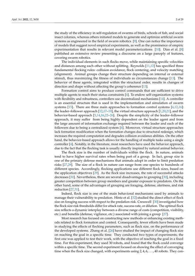
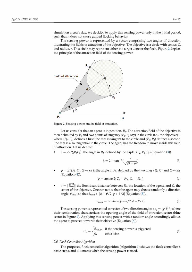
The sensing power is represented by a vector comprising two angles of directionillustrating the fields of attraction of the objective. The objective is a circle with center, C,and radius, r. This circle may represent either the target zone or the flock. Figure 2 depictsthe principle of the attraction field of the sensing power.

Figure 2. Sensing power and its field of attraction.

Let us consider that an agent is in position, P0. The attraction field of the objective isthen delimited by P0 and two points of tangency (P1, P2 say) in the circle (i.e., the objective)—where (P0, P1) defines a first line that is tangent to the circle and (P0, P2) defines a secondline that is also tangential to the circle. The agent has the freedom to move inside this fieldof attraction. Let us denote:

• θ = ](P2P0P1): the angle in P0, defined by the triplet (P2, P0, P1) (Equation (3)),

θ = 2× tan−1(r√

d2 − r2) (3)

• φ = ]((P0, C), X−axis): the angle in P0, defined by the two lines (P0, C) and X−axis(Equation (4)),

φ = arctan 2(Cy − P0y, Cx − P0x) (4)

• d = ‖−→P0C‖ the Euclidean distance between P0, the location of the agent, and C, thecenter of the objective. One can notice that the agent may choose randomly a directionangle, θrand, so that θrand ∈ [φ− θ/2, φ + θ/2] (Equation (5)).

θrand = random(φ− θ/2, φ + θ/2) (5)

The sensing power is represented as vector of two direction angles spi = [φ, θ]T , wheretheir combination characterizes the opening angle of the field of attraction sector (bluesector in Figure 2). Applying this sensing power with a random angle accordingly allowsthe agent to proceed towards their objective (Equation (6)).

ˆspi =

{θrand, if the sensing power is triggered0, otherwise

(6)

2.6. Flock Controller Algorithm

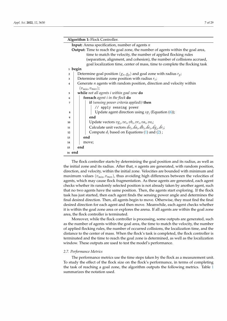
The proposed flock controller algorithm (Algorithm 1) shows the flock controller’sbasic steps, and illustrates when the sensing power is used.

Appl. Sci. 2022, 12, 3630 7 of 29

Algorithm 1: Flock Controller.Input: Arena specification, number of agents nOutput: Time to reach the goal zone, the number of agents within the goal area,

time to match the velocity, the number of applied flocking rules(separation, alignment, and cohesion), the number of collisions accrued,goal localization time, center of mass, time to complete the flocking task

1 begin2 Determine goal position (gx, gy) and goal zone with radius rg;3 Determine initiate zone position with radius rz;4 Generate n agents with random position, direction and velocity within

(vmin, vmax);5 while not all agents i within goal zone do6 foreach agent i in the flock do7 if (sensing power criteria applied)) then

// apply sensing power8 Update agent direction using spi (Equation (6));9 end

10 Update vectors vgi, vei, vbi, vri, vai, voi;11 Calculate unit vectors ˆdoi, ˆdai, ˆdbi, ˆdei, ˆdgi, ˆdri;12 Compute di based on Equations (1) and (2) ;13 end14 move;15 end16 end

The flock controller starts by determining the goal position and its radius, as well asthe initial zone and its radius. After that, n agents are generated, with random position,direction, and velocity, within the initial zone. Velocities are bounded with minimum andmaximum values (vmin, vmax), thus avoiding high differences between the velocities ofagents, which may cause flock fragmentation. As these agents are generated, each agentchecks whether its randomly selected position is not already taken by another agent, suchthat no two agents have the same position. Then, the agents start exploring. If the flocktask has just started, then each agent finds the sensing power angle and determines thefinal desired direction. Then, all agents begin to move. Otherwise, they must find the finaldesired direction for each agent and then move. Meanwhile, each agent checks whetherit is within the goal zone area or explores the arena. If all agents are within the goal zonearea, the flock controller is terminated.

Moreover, while the flock controller is processing, some outputs are generated, suchas the number of agents within the goal area, the time to match the velocity, the numberof applied flocking rules, the number of occurred collisions, the localization time, and thedistance to the center of mass. When the flock’s task is completed, the flock controller isterminated and the time to reach the goal zone is determined, as well as the localizationwindow. These outputs are used to test the model’s performance.

2.7. Performance Metrics

The performance metrics use the time steps taken by the flock as a measurement unit.To study the effect of the flock size on the flock’s performance, in terms of completingthe task of reaching a goal zone, the algorithm outputs the following metrics. Table 1summarizes the notation used.

Appl. Sci. 2022, 12, 3630 8 of 29

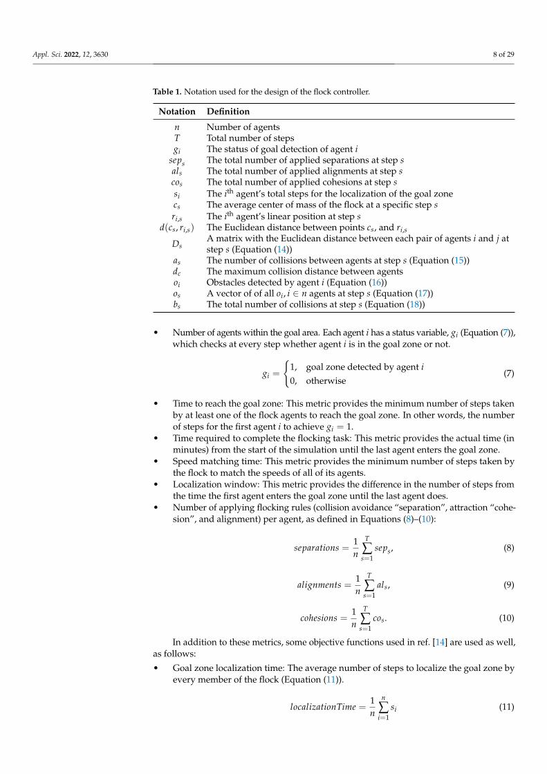
Table 1. Notation used for the design of the flock controller.

Notation Definition

n Number of agentsT Total number of stepsgi The status of goal detection of agent i

seps The total number of applied separations at step sals The total number of applied alignments at step scos The total number of applied cohesions at step ssi The ith agent’s total steps for the localization of the goal zonecs The average center of mass of the flock at a specific step sri,s The ith agent’s linear position at step s

d(cs, ri,s) The Euclidean distance between points cs, and ri,s

DsA matrix with the Euclidean distance between each pair of agents i and j atstep s (Equation (14))

as The number of collisions between agents at step s (Equation (15))dc The maximum collision distance between agentsoi Obstacles detected by agent i (Equation (16))os A vector of of all oi, i ∈ n agents at step s (Equation (17))bs The total number of collisions at step s (Equation (18))

• Number of agents within the goal area. Each agent i has a status variable, gi (Equation (7)),which checks at every step whether agent i is in the goal zone or not.

gi =

{1, goal zone detected by agent i0, otherwise

(7)

• Time to reach the goal zone: This metric provides the minimum number of steps takenby at least one of the flock agents to reach the goal zone. In other words, the numberof steps for the first agent i to achieve gi = 1.

• Time required to complete the flocking task: This metric provides the actual time (inminutes) from the start of the simulation until the last agent enters the goal zone.

• Speed matching time: This metric provides the minimum number of steps taken bythe flock to match the speeds of all of its agents.

• Localization window: This metric provides the difference in the number of steps fromthe time the first agent enters the goal zone until the last agent does.

• Number of applying flocking rules (collision avoidance “separation”, attraction “cohe-sion”, and alignment) per agent, as defined in Equations (8)–(10):

separations =1n

T

∑s=1

seps, (8)

alignments =1n

T

∑s=1

als, (9)

cohesions =1n

T

∑s=1

cos. (10)

In addition to these metrics, some objective functions used in ref. [14] are used as well,as follows:

• Goal zone localization time: The average number of steps to localize the goal zone byevery member of the flock (Equation (11)).

localizationTime =1n

n

∑i=1

si (11)

Appl. Sci. 2022, 12, 3630 9 of 29

• Average distance to the center of mass (Equation (12)), where the average center ofmass of the flock at each step, s, is defined by Equation (13):

distanceToCoM =1T

T

∑s=1

(1n

n

∑i=1

d(cs, ri,s)

), (12)

cs =1n

n

∑i=1

ri,s. (13)

• Collisions per member. This metric reports the number of collisions that occurredbetween agents and obstacles. The number of collisions as among all flock agents i,j at step s is computed based on the distances between them in Ds (Equation (14)),according to Equation (15).

Ds =

0 d12 . . . d1n

d21 0 . . . d2n...

.... . .

...dn1 dn2 . . . 0

, (14)

as =

{as + 1, dij ≤ dc, dij ∈ Ds, 1 ≤ i < j ≤ nas, otherwise.

(15)

Then, the collisions between agent i ∈ n and obstacles at step s are computed, asin Equations (16)–(18). Finally, the average number of collisions among the flockmembers and with obstacles is computed, as in Equation (19).

oi =

{1, obstacle detected within collision distance of agent i0, otherwise,

(16)

os = [o1, o2, . . . , on], (17)

bs =s

∑i=1

oi, oi ∈ os, (18)

collisions =1T

T

∑s=1

(as + bs). (19)

3. Results3.1. Simulation Environment

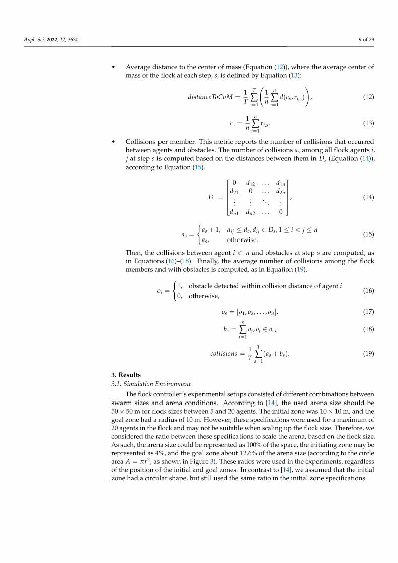
The flock controller’s experimental setups consisted of different combinations betweenswarm sizes and arena conditions. According to [14], the used arena size should be50× 50 m for flock sizes between 5 and 20 agents. The initial zone was 10× 10 m, and thegoal zone had a radius of 10 m. However, these specifications were used for a maximum of20 agents in the flock and may not be suitable when scaling up the flock size. Therefore, weconsidered the ratio between these specifications to scale the arena, based on the flock size.As such, the arena size could be represented as 100% of the space, the initiating zone may berepresented as 4%, and the goal zone about 12.6% of the arena size (according to the circlearea A = πr2, as shown in Figure 3). These ratios were used in the experiments, regardlessof the position of the initial and goal zones. In contrast to [14], we assumed that the initialzone had a circular shape, but still used the same ratio in the initial zone specifications.

Appl. Sci. 2022, 12, 3630 10 of 29

Figure 3. Arena specifications, including ratios.

Scaling up the arena requires more specification, in order to determine its size. Supposethat each agent occupies a 1 m2 size of the arena; this allows the maximum required spacefor an agent to be 50 × 50

20 = 125 m2 of the arena’s space. Therefore, using the properratio to calculate the suitable space of the arena is achieved by multiplying the maximumflock size by 125. In this work, we conducted experiments with flock sizes in the rangeof 10–100 agents in steps of 10. To ensure the containment of agents and obstacles, and tohave a standard environment for comparison, the arena specifications for the maximumflock size (100 agents) will be considered as follows: The arena size was 112× 112 m, theradius of the initial zone was 13 m, and the goal zone’s radius was 22 m. The experimentalparameters are summarized in Table 2.

Table 2. Simulation parameter values.

Parameter Value

n 10–100 agents in steps of 10Arena size 112× 112 m

Initiate zone radius 13 mGoal zone radius 22 m

Patch size 5.5× 5.5 pixels, corresponding to 1 m2

dc 0.55 patchstep 1 s

Agent speed Random number ∈[0–0.5] Patch∆r 1 patch∆o 13 patch∆a 1 patch

Priority weights w1 = 0.4, w2 = 0.075, w3 = 0.025

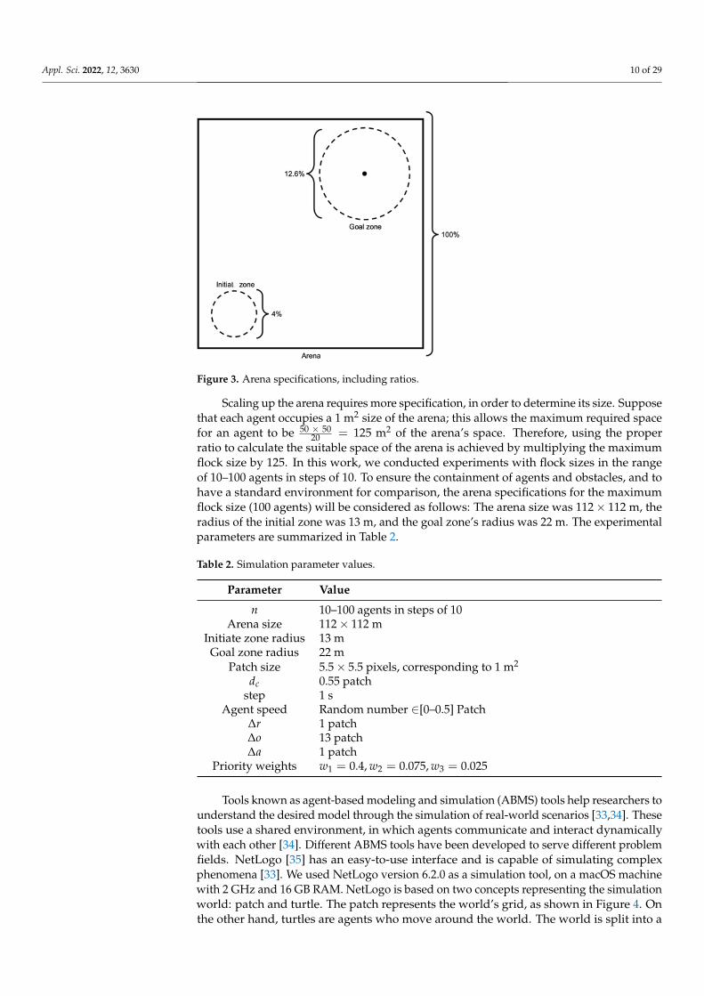
Tools known as agent-based modeling and simulation (ABMS) tools help researchers tounderstand the desired model through the simulation of real-world scenarios [33,34]. Thesetools use a shared environment, in which agents communicate and interact dynamicallywith each other [34]. Different ABMS tools have been developed to serve different problemfields. NetLogo [35] has an easy-to-use interface and is capable of simulating complexphenomena [33]. We used NetLogo version 6.2.0 as a simulation tool, on a macOS machinewith 2 GHz and 16 GB RAM. NetLogo is based on two concepts representing the simulationworld: patch and turtle. The patch represents the world’s grid, as shown in Figure 4. Onthe other hand, turtles are agents who move around the world. The world is split into a

Appl. Sci. 2022, 12, 3630 11 of 29

grid of patches, and is two-dimensional. Turtles may move across patches, described assquare pieces of “ground”. The patch size was set as 5.5× 5.5 pixels. Agents were set tofit a single patch size. On the other hand, the size of obstacles varied between one to twopatches [23]. Obstacles were added manually, as adding obstacles randomly to the arenamay lead to scenarios where the flock never applies obstacle avoidance. Collisions wereconsidered to occur when the distance between two agents (or an agent and an obstacle)was less than dc = 0.55.

Figure 4. Arena specifications ratio. The circle on the left displays an enlarged patch.

A time step does not directly map to real-world time (seconds). In our simulation, eachtime step varied between 0.095 and 0.973 s, based on the step length taken by the simulationcode. Therefore, we suppose that the time step interval is 1 s. Each agent initially has arandom speed. This random speed is assumed to be a floating number between 0 and 0.5.Hence, the movement of the agent could not exceed 0.5 patches ahead.

In contrast to [14], where various perception zones were used, we conducted multipletests to determine suitable common perception zones for all experimented flock sizes.Several zone sizes (∆r, ∆o, and ∆a) were tested on flock sizes of 30, 50, and 100 agents.Agent perception zone sizes were selected based on the results of these tests. The testresults considered goal zone localization time, the average distance to the center of mass,collisions per member, and the applied times of flocking rules. According to [14], a smallervalue of ∆r, and larger values of ∆o and ∆a led to better flocking behavior. However, therewere no precise ratios or constraints on the total perception radii. Therefore, a number ofzone sizes were tested (e.g., ∆r = 2, ∆o = 6, and ∆a = 7 for 30 agents) where the flockdid not show stable flocking behavior. To the contrary, the flock kept avoiding collisionbetween its members and maintained cohesion simultaneously. Therefore, we eliminatedthe sizes that caused a similar situation from the next test on bigger flock sizes (detailedresults provided in Appendix A). Experimentally, we found that smaller values of ∆r and∆a, and larger values of ∆o led to better flocking behavior. The final selected zones werethe minimum common sizes among all flock sizes that provided stable flocking behavior(∆r = 1, ∆o = 13, ∆a = 1). According to the arena specifications set earlier, the agent’sperception area covered 5.5% of the arena’s size. The repulsion priority weights w1, w2,and w3 (Equation (1)) were set according to reference [14] to allow for improved repulsionbehavior and to avoid having the desired position be too far from the agent, as follows:w1 = 0.4, w2 = 0.075, and w3 = 0.025.

3.2. Experimental Results

Each experiment was simulated 20 times (for 400 experiments in total) using NetLogo,and the obtained performance measures for each simulation were recorded. We reportthe average values obtained for each of the performance metrics over the twenty runs.Performance metric data for all simulations were analyzed using SPSS software [36].

Our aim is to explore the existence of an association between the change in flock size (asan independent variable) and each of the performance measures (as dependent variables).

Appl. Sci. 2022, 12, 3630 12 of 29

• We use regression curves to approximate the function or curve that has the best fit to anumber of observed data points in our experiments [37–39].

• The correlation coefficient, r ∈ [−1, 1], describes the relationship and measures thestrength of the association between two variables, and is defined in Equation (20) [40],where m is the sample size (i.e., the number of experiments), x is the value of theindependent variable (i.e., the flock size), and y is the value of the dependent variable(i.e., the performance metric).

• The coefficient of determination, R2 ∈ [0, 1], explains the variations in the performancemeasure accounted for by flock size. It is obtained by squaring the r value and isnormally expressed as a percentage in the interpretation of results. An R2 close to0 reflects a model that does not explain the change in the performance measure aroundits mean, while an R2 close to 1 reflects a model that explains all the variation of theperformance measure around its mean due to change in the flock size.

• The p-value tests the null hypothesis, which states that there is no association betweenchanges in the flock size and shifts in the performance measure. If the p-value isless than the significance level α, then it indicates that the data from the experimentsprovides enough evidence to reject the null hypothesis.

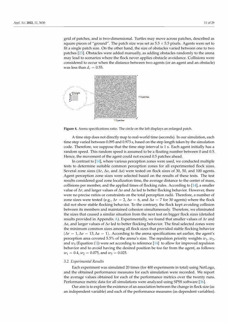
• The distribution of data points in the scatter plots shown in Figures 5 and 6 are ob-tained from the experiments and are estimated for each of the six functions generatedby the SPSS statistical software (linear, inverse, logarithmic, quadratic, cubic, andexponential). The R2 for each of these functions allows us to determine the associationbetween the flock size and each of the performance measures.

r =m ∑ xy−∑ x ∑ y√

[m ∑ x2 − (∑ x)2√

m ∑ y2 − (∑ y)2, (20)

The remainder of this section is organized as follows: Section 3.2.1 reports the resultsof experiments excluding obstacles. Next, Section 3.2.2 reports the results of experimentsincluding obstacles. All of the experiments used the settings and parameters described inTable 2.

(a) (b)

(c) (d)

Figure 5. Cont.

Appl. Sci. 2022, 12, 3630 13 of 29

(e) (f)

(g) (h)

(i)

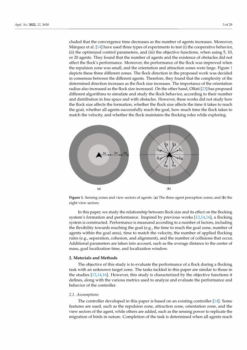
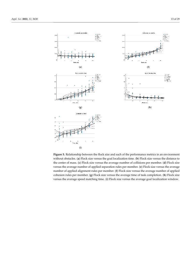
Figure 5. Relationship between the flock size and each of the performance metrics in an environmentwithout obstacles. (a) Flock size versus the goal localization time. (b) Flock size versus the distance tothe center of mass. (c) Flock size versus the average number of collisions per member. (d) Flock sizeversus the average number of applied separation rules per member. (e) Flock size versus the averagenumber of applied alignment rules per member. (f) Flock size versus the average number of appliedcohesion rules per member. (g) Flock size versus the average time of task completion. (h) Flock sizeversus the average speed matching time. (i) Flock size versus the average goal localization window.

Appl. Sci. 2022, 12, 3630 14 of 29

(a) (b)

(c) (d)

(e) (f)

(g) (h)

(i)

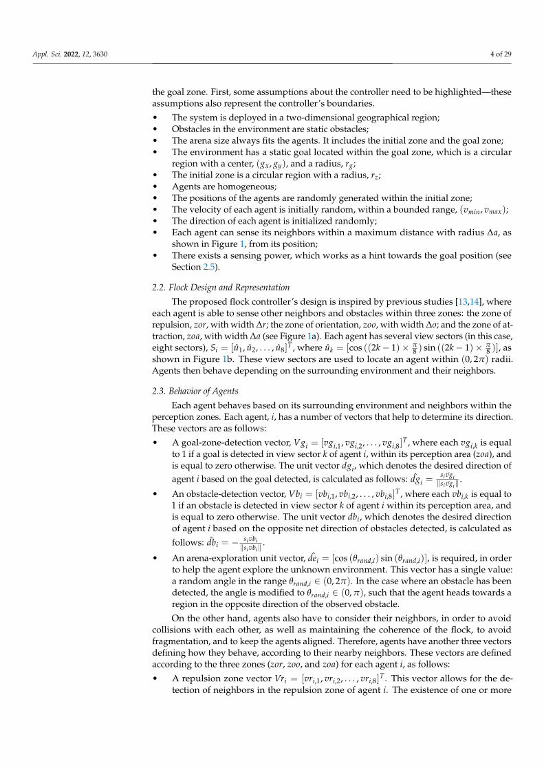
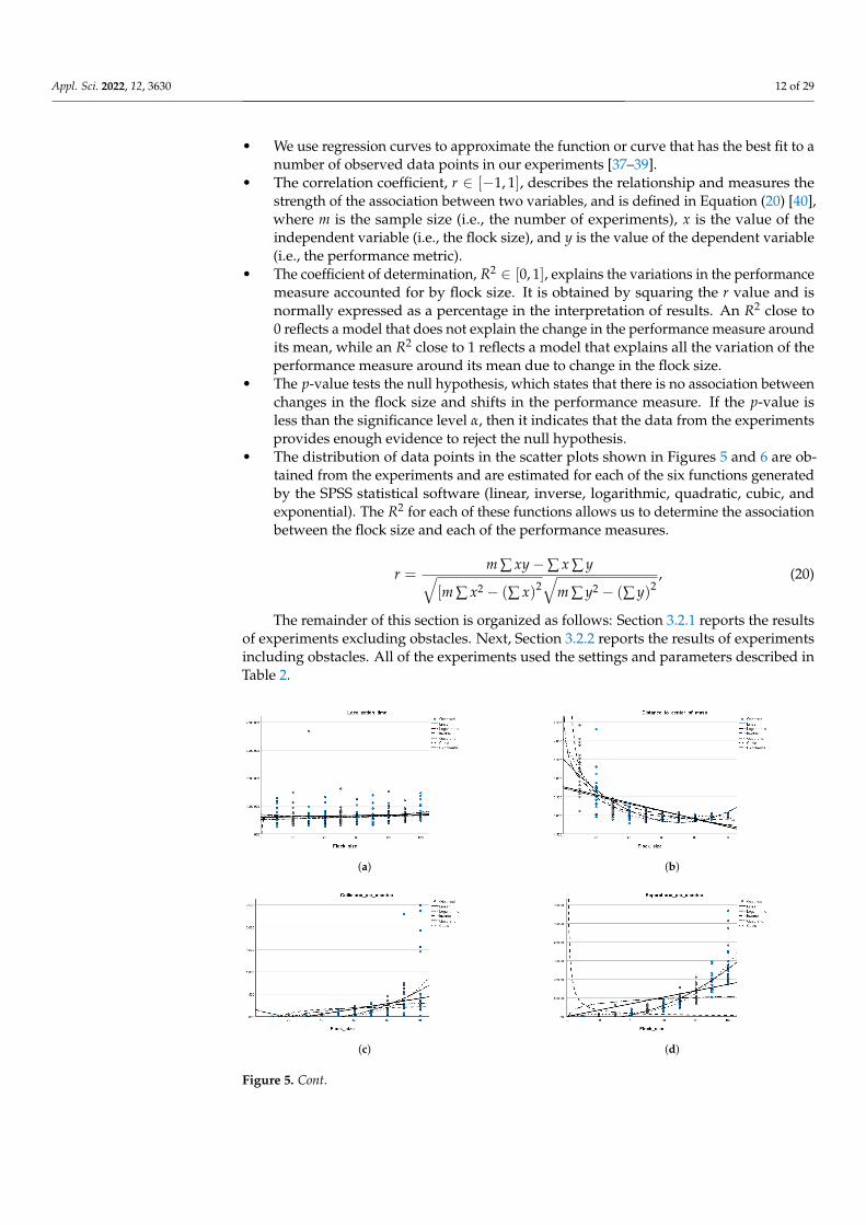
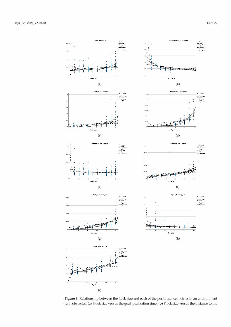
Figure 6. Relationship between the flock size and each of the performance metrics in an environmentwith obstacles. (a) Flock size versus the goal localization time. (b) Flock size versus the distance to the

Appl. Sci. 2022, 12, 3630 15 of 29

center of mass. (c) Flock size versus the average number of collisions per member. (d) Flock sizeversus the average number of applied separation rules per member. (e) Flock size versus the averagenumber of applied alignment rules per member. (f) Flock size versus the average number of appliedcohesion rules per member. (g) Flock size versus the average time of task completion. (h) Flock sizeversus the average speed matching time. (i) Flock size versus the average goal localization window.

3.2.1. Experimental Results in an Environment without Obstacles

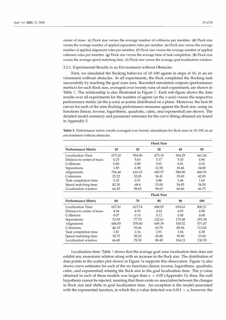
First, we simulated the flocking behavior of 10–100 agents in steps of 10, in an en-vironment without obstacles. In all experiments, the flock completed the flocking tasksuccessfully by reaching the goal zone area. Recorded simulation outputs (performancemetrics) for each flock size, averaged over twenty runs of each experiment, are shown inTable 3. The relationship is also illustrated in Figure 5. Each sub-figure shows the dataresults over all experiments for the number of agents (at the x-axis) versus the respectiveperformance metric (at the y-axis) as points distributed on a plane. Moreover, the best-fitcurves for each of the nine flocking performance measures against the flock size, using sixfunctions (linear, inverse, logarithmic, quadratic, cubic, and exponential) are shown. Thedetailed model summary and parameter estimates for the curve fitting obtained are foundin Appendix B.

Table 3. Performance metric results averaged over twenty simulations for flock sizes in 10–100, in anenvironment without obstacles.

Flock Size

Performance Metric 10 20 30 40 50

Localization Time 673.20 594.96 673.19 564.29 661.26Distance to center of mass 6.25 5.63 5.17 5.03 4.96Collisions 0.00 0.00 0.01 0.01 0.03Separations 1.85 6.98 12.58 18.46 34.80Alignments 706.40 616.23 690.57 580.90 668.76Cohesions 25.22 32.85 34.41 35.83 42.83Task completion time 0.30 0.51 0.88 1.06 1.65Speed matching time 82.30 68.6 33.00 54.85 34.50Localization window 66.45 58.65 58.65 60.60 66.75

Flock Size



Localization time: Table 3 shows that the average goal zone localization time does notexhibit any monotonic relation along with an increase in the flock size. The distribution ofdata points in the scatter plot shown in Figure 5a supports this observation. Figure 5a alsoshows curve estimates for each of the six functions (linear, inverse, logarithmic, quadratic,cubic, and exponential) relating the flock size to the goal localization time. The p-valueobtained in each of these models was larger than α = 0.05 (Appendix B); thus, the nullhypothesis cannot be rejected, meaning that there exists no association between the changesin flock size and shifts in goal localization time. An exception is the model associatedwith the exponential function, in which the p-value detected was 0.011 < α; however, the

Appl. Sci. 2022, 12, 3630 16 of 29

associated R2 value indicates that the only 3.2% of the variation in the localization time isexplained by the flock size.

Distance to center of mass: The average distance to center of mass values tend todecrease along with the increase in the flock size (Table 3 and Figure 5b). The flockingbehavior is exhibited here, where a larger flock size enables more members to be containedin a flocking zone, allowing the average distance to the center of mass to be reduced.Figure 5b also shows curve estimates for each of the six functions relating the flock sizeto the distance to center of mass. The p-value obtained for each of these models was lessthan 0.001, which means that the sample data provides enough evidence to reject the nullhypothesis, and that changes in the flock size are significantly associated with shifts inthe distance to center of mass, on the population level. The R2 value associated with theinverse function for the distance to the center of mass indicates that 69.7% of the variationin the distance to center of mass is explained by the flock size, while the R2 value associatedwith the cube function was somewhat higher than that, at 71.1%.

Speed matching time: A similar observation of distance to center of mass can be drawnfor the speed matching time measure. Figure 5h shows curve estimates for each of the sixfunctions relating the flock size to the speed matching time. The p-value obtained for eachof these models was less than 0.001, which means that the sample data provides enoughevidence to reject the null hypothesis, and that changes in the flock size are significantlyassociated with shifts in the speed matching time on the population level. For the speedmatching time, the highest R2 value is that associated with the inverse function and itaccounted for only 12.3% of the variation in speed matching time due to changes in theflock size.

Collisions per member: The average collisions per member tend to increase along withthe increase in the flock size as shown in Table 3. The number of collision avoidance stepsneeded for a larger flock size is larger than the number needed for a smaller flock size. Thescatter plot in Figure 5c also shows that the standard deviation is small (2.5 collisions). Thep-value obtained in each of the six curve estimation models was less than 0.001, whichmeans that the sample data provides enough evidence to reject the null hypothesis, and thatchanges in the flock size are significantly associated with shifts in the number of collisionson the population level. However, the R2 values associated with these models are a bitlower than those obtained for the models of the distance to center of mass variable. TheR2 value associated with the quadratic function indicates that 31.5% of the variation in thenumber of collisions is explained by the flock size, while the R2 value associated with thecube function was closely higher than that at 33.7%.

Separations per member: Table 3 shows a steady increase in the average numberof applied separation steps along with the increase in the flock size. The scatter plot inFigure 5d) clearly supports that. The shape of the scatter is close to a quadratic or a cubicfunction. In fact, the p-value obtained in each of the six curve estimation models was lessthan 0.001, which means that the sample data provides enough evidence to reject the nullhypothesis, and that changes in flock size are significantly associated with shifts in thenumber of applied separation steps on the population level. The highest R2 value is thatassociated with the cubic function (81.4%), closely followed by the R2 value associated withthe quadratic function at 79.5%.

Alignments per member: Similar to goal localization time, Table 3 shows that theaverage number of alignment steps does not exhibit any monotonic relation along withan increase in the flock size. The distribution of data points in the scatter plot shown inFigure 5e supports this observation. It appears that the average number of alignment stepsper member is not affected by the flock size. The scatter of data points appears in everyflock size. Figure 5e also shows curve estimates for each of the six functions relating theflock size to the average number of alignment steps per member. The p-value obtainedin each of these models was larger than α = 0.05 (Appendix B); thus, the null hypothesiscannot be rejected, meaning that there exists no association between changes in flock sizeand shifts in the number of alignment steps.

Appl. Sci. 2022, 12, 3630 17 of 29

Cohesions per member: The average cohesion steps per member monotonically in-creases with the increase in the flock size as shown in Table 3, which is confirmed bythe scatter plot in Figure 5f. The distribution of data points in the scatter plot shown inFigure 5f shows that the standard deviation of number of cohesion steps is similar foreach flock size; however, the average number of cohesion steps increases as the flock sizeincreases. The number of cohesion steps needed to keep a larger flock size in cohesion islarger than the number needed for a smaller flock size. The p-value obtained in each ofthe six curve estimation models was less than 0.001, which means that the sample dataprovides enough evidence to reject the null hypothesis, and that changes in flock size aresignificantly associated with shifts in the number of cohesion steps on the population level.The highest R2 value is that associated with the cubic function and explains 87.2% of thevariation in the number of cohesion steps due to shifts in the flock size.

Task completion time and goal localization window: The time required to completethe task in minutes (Figure 5g), as well as the goal localization window (Figure 5i) allincreased along with an increase in flock size, as supported by the average value readingsfrom Table 3. The p-value obtained in each of the six curve estimation models for bothof these metrics was less than 0.001, which means that the sample data provides enoughevidence to reject the null hypothesis and that changes in flock size are strongly associatedwith shifts in each of these two performance measures. For the time required to completethe task measure, the highest R2 value was associated with the exponential function andaccounted for 80.2% of the variation in time required to complete the flocking task due tochanges in the flock size. As for the goal localization window, the highest R2 value wasassociated with the cubic function and indicates that 75.5% of the variation in the goallocalization window is explained by changes in the flock size, while the R2 value associatedwith the quadratic function closely follows at 75.2%. These results are in line with the shapeof the points on the scatter plot in Figure 5i.

As previously mentioned, the flocking behavior became stable when the majority ofthe flock members applied the alignment rule, rather than the attraction or separation rules.Based on the obtained results, the larger the flock size, the larger the number of repulsionand cohesion steps applied. The simulation outputs of two randomly selected experimentswith flock sizes of 30 and 100 are shown in Appendix C.

3.2.2. Experimental Results in an Environment with Obstacles

Next, experiments simulating the flocking behavior of 10–100 agents in steps of 10,in an environment with obstacles are conducted. In all experiments, the flock was ableto complete the flocking task successfully by reaching the goal zone area. Recordedsimulation outputs (performance metrics) for each flock size, averaged over twenty runs ofeach experiment, are shown in Table 4. The relationships are also illustrated in Figure 6.Each sub-figure shows the data results over all experiments for the number of agents (onthe x-axis) versus the respective performance metric (on the y-axis) as points distributed ona plane. Moreover, the best-fit curves for each of the nine flocking performance measuresagainst the flock size, using six functions (linear, inverse, logarithmic, quadratic, cubic, andexponential) are shown. The detailed model summary and parameter estimates for thecurve fitting obtained are found in Appendix B.

Appl. Sci. 2022, 12, 3630 18 of 29

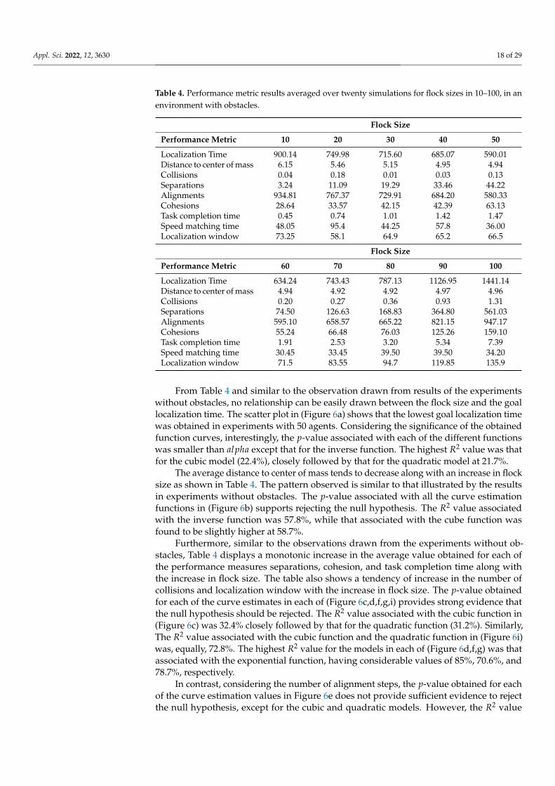
Table 4. Performance metric results averaged over twenty simulations for flock sizes in 10–100, in anenvironment with obstacles.

Flock Size



Flock Size



From Table 4 and similar to the observation drawn from results of the experimentswithout obstacles, no relationship can be easily drawn between the flock size and the goallocalization time. The scatter plot in (Figure 6a) shows that the lowest goal localization timewas obtained in experiments with 50 agents. Considering the significance of the obtainedfunction curves, interestingly, the p-value associated with each of the different functionswas smaller than alpha except that for the inverse function. The highest R2 value was thatfor the cubic model (22.4%), closely followed by that for the quadratic model at 21.7%.

The average distance to center of mass tends to decrease along with an increase in flocksize as shown in Table 4. The pattern observed is similar to that illustrated by the resultsin experiments without obstacles. The p-value associated with all the curve estimationfunctions in (Figure 6b) supports rejecting the null hypothesis. The R2 value associatedwith the inverse function was 57.8%, while that associated with the cube function wasfound to be slightly higher at 58.7%.

Furthermore, similar to the observations drawn from the experiments without ob-stacles, Table 4 displays a monotonic increase in the average value obtained for each ofthe performance measures separations, cohesion, and task completion time along withthe increase in flock size. The table also shows a tendency of increase in the number ofcollisions and localization window with the increase in flock size. The p-value obtainedfor each of the curve estimates in each of (Figure 6c,d,f,g,i) provides strong evidence thatthe null hypothesis should be rejected. The R2 value associated with the cubic function in(Figure 6c) was 32.4% closely followed by that for the quadratic function (31.2%). Similarly,The R2 value associated with the cubic function and the quadratic function in (Figure 6i)was, equally, 72.8%. The highest R2 value for the models in each of (Figure 6d,f,g) was thatassociated with the exponential function, having considerable values of 85%, 70.6%, and78.7%, respectively.

In contrast, considering the number of alignment steps, the p-value obtained for eachof the curve estimation values in Figure 6e does not provide sufficient evidence to rejectthe null hypothesis, except for the cubic and quadratic models. However, the R2 value

Appl. Sci. 2022, 12, 3630 19 of 29

associated with these models can only explain the variation in no more than 8.5% of thenumber of alignment steps due to the change in flock size.

Finally, the average speed matching time values reported in Table 4 do not show aclear relationship with the flock size. However, the p-value for all the curve estimationfunctions in Figure 6h for this measure show strong evidence to reject the null hypothesis.Notably, the highest R2 value obtained from these functions can explain no more than 6.5%of the change in the speed matching time due to the change in flock size.

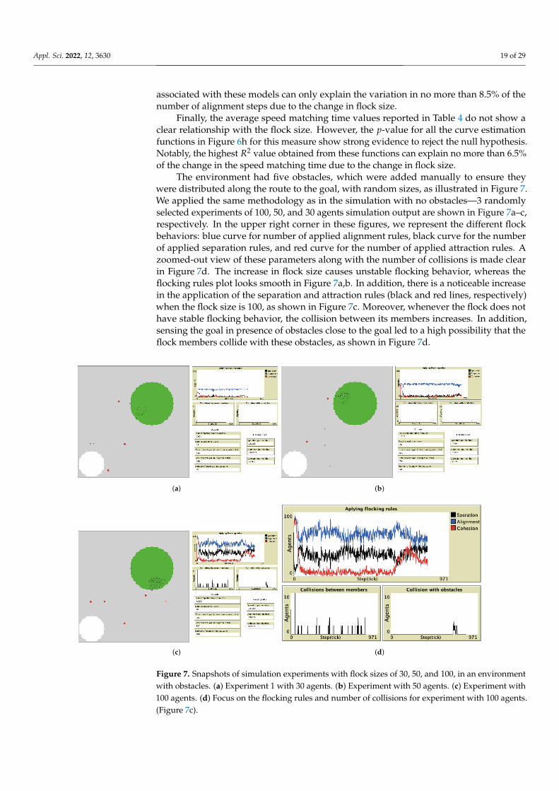
The environment had five obstacles, which were added manually to ensure theywere distributed along the route to the goal, with random sizes, as illustrated in Figure 7.We applied the same methodology as in the simulation with no obstacles—3 randomlyselected experiments of 100, 50, and 30 agents simulation output are shown in Figure 7a–c,respectively. In the upper right corner in these figures, we represent the different flockbehaviors: blue curve for number of applied alignment rules, black curve for the numberof applied separation rules, and red curve for the number of applied attraction rules. Azoomed-out view of these parameters along with the number of collisions is made clearin Figure 7d. The increase in flock size causes unstable flocking behavior, whereas theflocking rules plot looks smooth in Figure 7a,b. In addition, there is a noticeable increasein the application of the separation and attraction rules (black and red lines, respectively)when the flock size is 100, as shown in Figure 7c. Moreover, whenever the flock does nothave stable flocking behavior, the collision between its members increases. In addition,sensing the goal in presence of obstacles close to the goal led to a high possibility that theflock members collide with these obstacles, as shown in Figure 7d.

(a) (b)

(c) (d)

Figure 7. Snapshots of simulation experiments with flock sizes of 30, 50, and 100, in an environmentwith obstacles. (a) Experiment 1 with 30 agents. (b) Experiment with 50 agents. (c) Experiment with100 agents. (d) Focus on the flocking rules and number of collisions for experiment with 100 agents.(Figure 7c).

Appl. Sci. 2022, 12, 3630 20 of 29

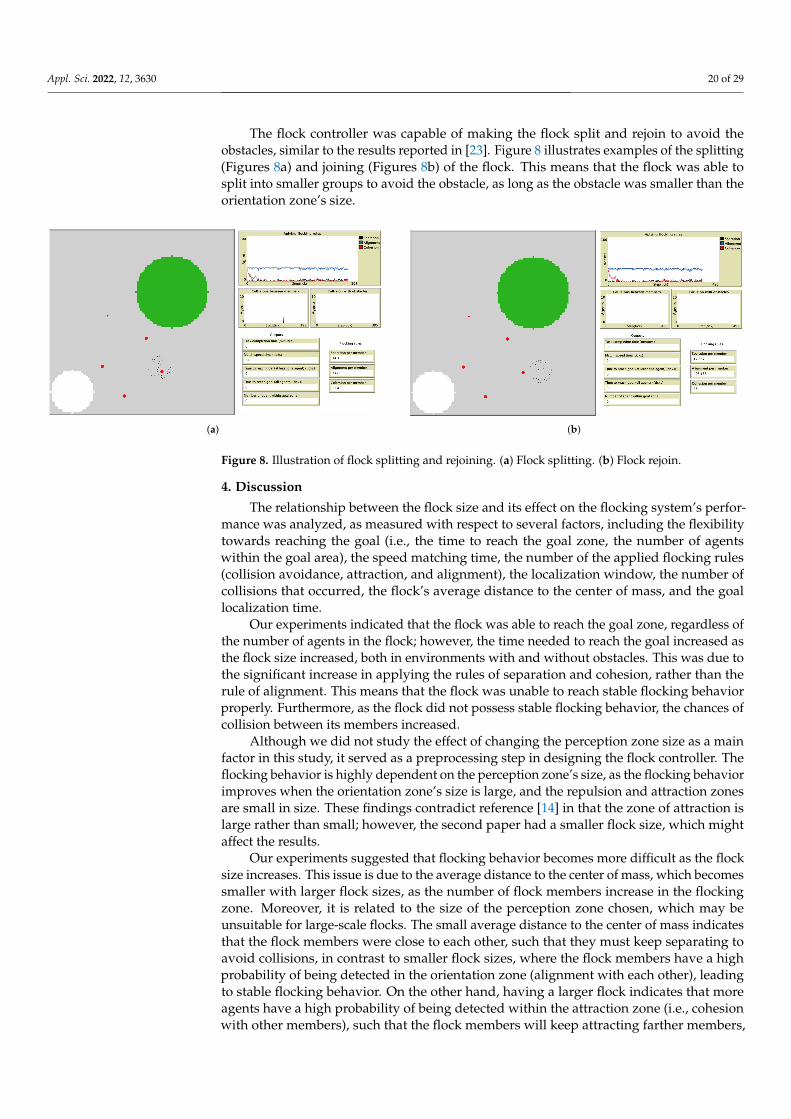
The flock controller was capable of making the flock split and rejoin to avoid theobstacles, similar to the results reported in [23]. Figure 8 illustrates examples of the splitting(Figures 8a) and joining (Figures 8b) of the flock. This means that the flock was able tosplit into smaller groups to avoid the obstacle, as long as the obstacle was smaller than theorientation zone’s size.

(a) (b)

Figure 8. Illustration of flock splitting and rejoining. (a) Flock splitting. (b) Flock rejoin.

4. Discussion

The relationship between the flock size and its effect on the flocking system’s perfor-mance was analyzed, as measured with respect to several factors, including the flexibilitytowards reaching the goal (i.e., the time to reach the goal zone, the number of agentswithin the goal area), the speed matching time, the number of the applied flocking rules(collision avoidance, attraction, and alignment), the localization window, the number ofcollisions that occurred, the flock’s average distance to the center of mass, and the goallocalization time.

Our experiments indicated that the flock was able to reach the goal zone, regardless ofthe number of agents in the flock; however, the time needed to reach the goal increased asthe flock size increased, both in environments with and without obstacles. This was due tothe significant increase in applying the rules of separation and cohesion, rather than therule of alignment. This means that the flock was unable to reach stable flocking behaviorproperly. Furthermore, as the flock did not possess stable flocking behavior, the chances ofcollision between its members increased.

Although we did not study the effect of changing the perception zone size as a mainfactor in this study, it served as a preprocessing step in designing the flock controller. Theflocking behavior is highly dependent on the perception zone’s size, as the flocking behaviorimproves when the orientation zone’s size is large, and the repulsion and attraction zonesare small in size. These findings contradict reference [14] in that the zone of attraction islarge rather than small; however, the second paper had a smaller flock size, which mightaffect the results.

Our experiments suggested that flocking behavior becomes more difficult as the flocksize increases. This issue is due to the average distance to the center of mass, which becomessmaller with larger flock sizes, as the number of flock members increase in the flockingzone. Moreover, it is related to the size of the perception zone chosen, which may beunsuitable for large-scale flocks. The small average distance to the center of mass indicatesthat the flock members were close to each other, such that they must keep separating toavoid collisions, in contrast to smaller flock sizes, where the flock members have a highprobability of being detected in the orientation zone (alignment with each other), leadingto stable flocking behavior. On the other hand, having a larger flock indicates that moreagents have a high probability of being detected within the attraction zone (i.e., cohesionwith other members), such that the flock members will keep attracting farther members,

Appl. Sci. 2022, 12, 3630 21 of 29

according to their perception, while avoiding collisions with closer members within therepulsion zone which, in turn, results in unstable flocking behavior.

As the flock size increases, so do the number of collisions, cohesion, and separations.This is expected because of the increase in probability of these events as the number offlock members increases. An increase in the scatter for larger flock sizes can be similarlyobserved. The increase in flock size creates a more complex environment for the flock tonavigate, resulting in a larger variance of flock behavior.

Our findings indicated that the speed matching time slightly decreased along with anincrease in the number of agents in an environment without obstacles. On the other hand,the speed matching time was slightly increased in the environments with obstacles. Thismeans that obstacles affect the time to reach the goal, as they hinder exploration. However,the reach time was logically affected by the average speed of the flock. Speed matchingtime has a larger scatter as the flock size decreases. This is because there are fewer flockmembers overall within the attraction zone of each flock member, compared with largerflock sizes. The results of reference [14] support our findings, in that each agent’s finaldesired direction becomes more complicated and takes more time to determine as thesize increases.

From our findings we observed that as the flock size increases, the time requiredto complete the task increases as well, which does not adhere to reference [14]. Thisdiscordance is due to the fact that the flock sizes used in their work (with a maximum flocksize of 20) were much smaller than the flock sizes used in this work. Moreover, the increasein the time required to complete the task is due to the formation maintenance and cohesionof flock members, which prevents the flock from exploring the environment properly(i.e., presenting stable flocking behavior). Interestingly, the average goal localization timeremained unaffected by the flock size, further supporting that an increase in flock sizerequires higher formation maintenance behavior.

To summarize, flock size does not significantly affect localization time and the numberof alignments per flock member. Scatter is homogeneous for all flock sizes. An increase inflock size is positively associated with the number of collisions, separations, and cohesionsper flock member. In addition, the localization window and task completion times bothincrease as flock size increases, and and increase in variability or scatter is seen as well.A decrease in flock size is associated with a larger distance to the center of mass of theflock, as well as larger and more variable speed matching times. Scatter increases with thedecrease in flock size.

The results we obtained highlight the critical factors that are affected by changing theflock size, and are expected to be helpful for future research in this field. The limitationsof this work lie in the small number of experiments conducted for each flock size due totime constraints. In addition, a sample size of 20 makes it difficult to draw conclusionsregarding the apparent outliers in the data, as well as the standard deviation for each flocksize. The excessive runtime required for larger flock sizes further prohibits experimentsbeyond 100 flock members. Furthermore, the controller used in this work may not be fullygeneralizable to other flocking tasks.

5. Conclusions

In this paper, we studied the impact of changing the flock size on the performance ofthe flock task. We developed a flock controller using a behavior-based swarm approachand conducted experiments on the problem of reaching a goal zone. Our flock controllerdepends on the behavior of a flock’s agents, with respect to their neighbors and to theenvironment. Moreover, the flock controller also introduces the concept of sensing powerthat replicates the phenomenon observed in nature where migrating birds have a sense ofwhere they need to head, even if they do not precisely know the target. The sensing powerprovides better take-off results.

In this work, we studied the impact of flock size on flock formation and flock perfor-mance through nine different parameters, including the goal zone localization time, the

Appl. Sci. 2022, 12, 3630 22 of 29

distance to the center of mass, the collisions per member, and the rate of application of theflocking rules. These parameters were measured for ten flocks with increasing size. Theflocking behavior was simulated in two different environments, with and without obstacles.The results demonstrated that the developed flock controller is able to deliver the flockto the goal zone, regardless of its size. The experiments concluded that the time requiredto complete the task in minutes, and the goal localization window increased along withan increase in flock size. The same behavior was observed for the average collisions permember, the average number of applied separations, and the average number of cohesionsteps. On the contrary, the results also concluded that the average distance to center ofmass, as well as the speed matching time, tend to decrease along with the increase in theflock size. We also observed that the remaining analyzed parameters, namely the goallocalization time and the number of applied alignment steps, had no clear association withthe variations in the flock size. Overall, similar results were observed in both situationswith and without obstacles.

As mentioned above, spatial organization is an area where behavior-based swarmapproaches can be applied. This paper studied the impact of the number of agents on thedifferent parameters involved in moving individual robots to spatially organize themselvesin a specific region of the environment. As the number of collisions and separations tendsto increase with the number of involved agents and certainly impacts the time requiredto complete the task, in future studies, we intend to work on minimizing the collisionsamong agents in order to improve the task completion time. We will also study the impactof using the sensing power continuously for motion coordination among the flock and toimprove the navigation process. Moreover, the flock controller may integrate other featuresto memorize discovered areas, which could help reduce the time required to reach the goal.

Author Contributions: Conceptualization, A.T. and R.A.; methodology, S.A. and N.A.; software,R.A.; validation, A.T., R.A., and S.Q.; formal analysis, S.A. and N.A.;writing—original draft prepa-ration, S.A. and R.A.; writing—review and editing, S.A., A.T., S.Q. and N.A.; visualization, R.A.;supervision, A.T.; project administration, S.Q.; funding acquisition, S.Q. All authors have read andagreed to the published version of the manuscript.

Funding: This work was funded by the National Plan for Science, Technology and Innovation(MAARIFAH), King Abdulaziz City for Science and Technology, Kingdom of Saudi Arabia, AwardNumber (13-SPA1130-02).

Institutional Review Board Statement: Not applicable.

Informed Consent Statement: Not applicable.

Data Availability Statement: Not applicable.

Acknowledgments: The authors would like to thank the anonymous reviewers for their construc-tive comments. Special thanks to Najla Elhazzani from the Department of Statistics and OperationsResearch, College of Science, King Saud University for her useful comments.

Conflicts of Interest: The authors declare no conflict of interest. The funders had no role in the designof the study; in the collection, analyses, or interpretation of data; in the writing of the manuscript, orin the decision to publish the results.

Appendix A

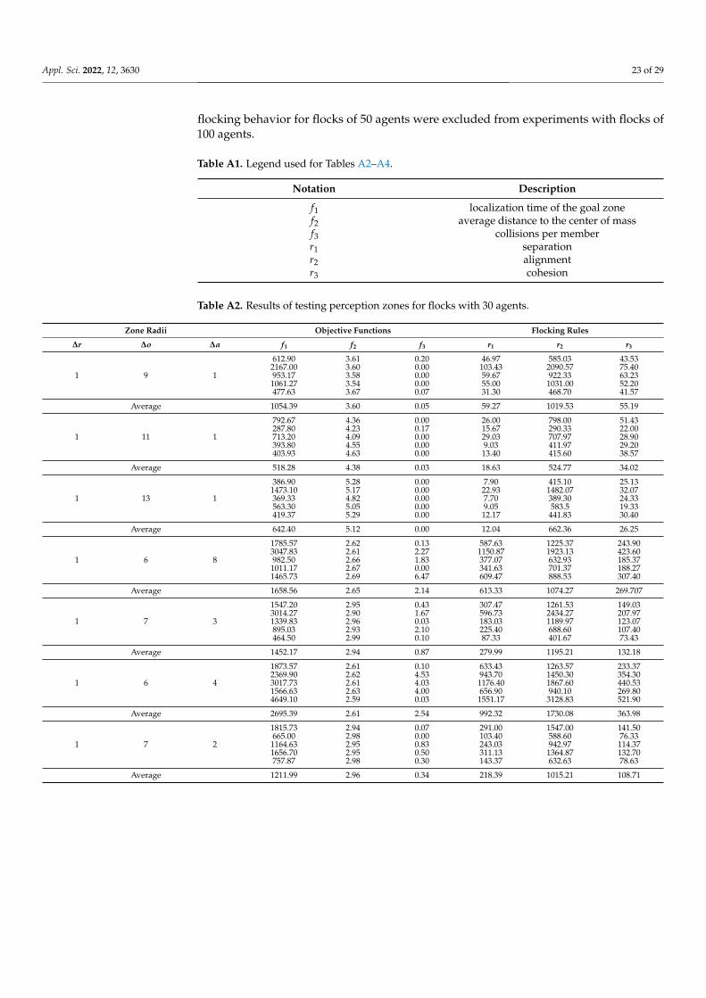
This appendix provides details on the tuning of the repulsion orientation and tests forattraction zone radii for flocks with 30, 50, and 100 agents. Table A1 shows the legend usedin the results provided in Tables A2–A4. For each used combination of ∆r, ∆o, and ∆a, theobtained objective functions f1, f2, and f3 are shown, along with the number of repulsionoperations (r1), the number of alignment operations (r2), and the number of cohesionoperations (r3) encountered. Combinations of ∆r, ∆o, and ∆a that resulted in unstableflocking behavior for flocks of 30 agents were excluded from experiments consideringflocks of 50 agents. Similarly, combinations of ∆r, ∆o, and ∆a that resulted in unstable

Appl. Sci. 2022, 12, 3630 23 of 29

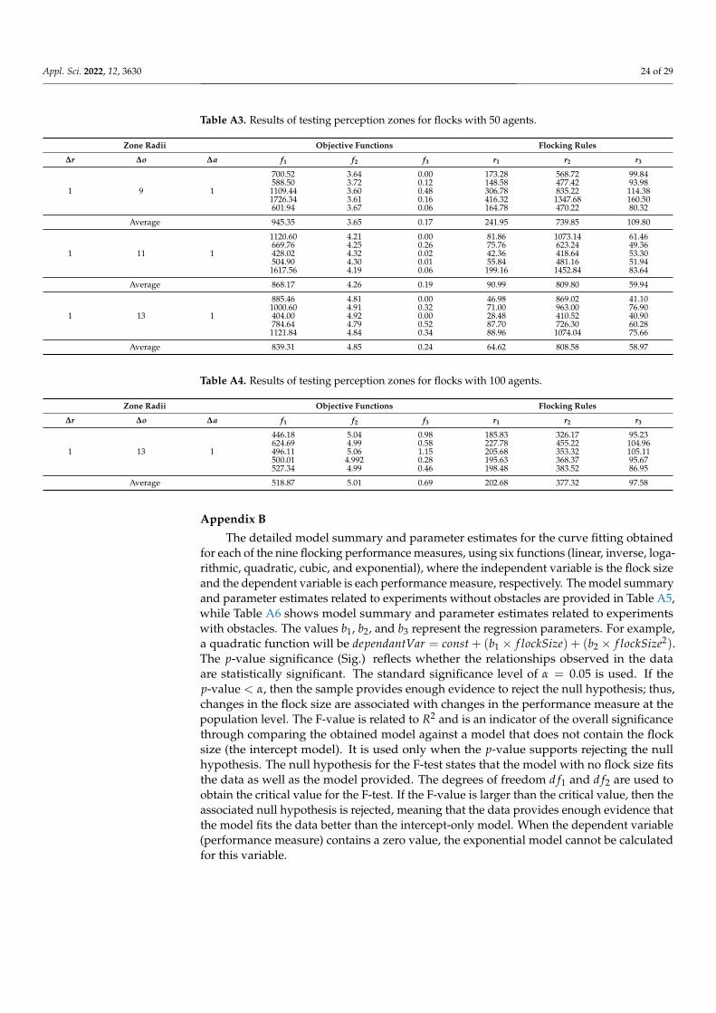
flocking behavior for flocks of 50 agents were excluded from experiments with flocks of100 agents.

Table A1. Legend used for Tables A2–A4.

Notation Description

f1 localization time of the goal zonef2 average distance to the center of massf3 collisions per memberr1 separationr2 alignmentr3 cohesion

Table A2. Results of testing perception zones for flocks with 30 agents.

Zone Radii Objective Functions Flocking Rules

∆r ∆o ∆a f1 f2 f3 r1 r2 r3

1 9 1

612.90 3.61 0.20 46.97 585.03 43.532167.00 3.60 0.00 103.43 2090.57 75.40953.17 3.58 0.00 59.67 922.33 63.231061.27 3.54 0.00 55.00 1031.00 52.20477.63 3.67 0.07 31.30 468.70 41.57

Average 1054.39 3.60 0.05 59.27 1019.53 55.19

1 11 1

792.67 4.36 0.00 26.00 798.00 51.43287.80 4.23 0.17 15.67 290.33 22.00713.20 4.09 0.00 29.03 707.97 28.90393.80 4.55 0.00 9.03 411.97 29.20403.93 4.63 0.00 13.40 415.60 38.57

Average 518.28 4.38 0.03 18.63 524.77 34.02

1 13 1

386.90 5.28 0.00 7.90 415.10 25.131473.10 5.17 0.00 22.93 1482.07 32.07369.33 4.82 0.00 7.70 389.30 24.33563.30 5.05 0.00 9.05 583.5 19.33419.37 5.29 0.00 12.17 441.83 30.40

Average 642.40 5.12 0.00 12.04 662.36 26.25

1 6 8

1785.57 2.62 0.13 587.63 1225.37 243.903047.83 2.61 2.27 1150.87 1923.13 423.60982.50 2.66 1.83 377.07 632.93 185.371011.17 2.67 0.00 341.63 701.37 188.271465.73 2.69 6.47 609.47 888.53 307.40

Average 1658.56 2.65 2.14 613.33 1074.27 269.707

1 7 3

1547.20 2.95 0.43 307.47 1261.53 149.033014.27 2.90 1.67 596.73 2434.27 207.971339.83 2.96 0.03 183.03 1189.97 123.07895.03 2.93 2.10 225.40 688.60 107.40464.50 2.99 0.10 87.33 401.67 73.43

Average 1452.17 2.94 0.87 279.99 1195.21 132.18

1 6 4

1873.57 2.61 0.10 633.43 1263.57 233.372369.90 2.62 4.53 943.70 1450.30 354.303017.73 2.61 4.03 1176.40 1867.60 440.531566.63 2.63 4.00 656.90 940.10 269.804649.10 2.59 0.03 1551.17 3128.83 521.90

Average 2695.39 2.61 2.54 992.32 1730.08 363.98

1 7 2

1815.73 2.94 0.07 291.00 1547.00 141.50665.00 2.98 0.00 103.40 588.60 76.331164.63 2.95 0.83 243.03 942.97 114.371656.70 2.95 0.50 311.13 1364.87 132.70757.87 2.98 0.30 143.37 632.63 78.63

Average 1211.99 2.96 0.34 218.39 1015.21 108.71

Appl. Sci. 2022, 12, 3630 24 of 29



∆r ∆o ∆a f1 f2 f3 r1 r2 r3

1 9 1

700.52 3.64 0.00 173.28 568.72 99.84588.50 3.72 0.12 148.58 477.42 93.981109.44 3.60 0.48 306.78 835.22 114.381726.34 3.61 0.16 416.32 1347.68 160.50601.94 3.67 0.06 164.78 470.22 80.32

Average 945.35 3.65 0.17 241.95 739.85 109.80

1 11 1

1120.60 4.21 0.00 81.86 1073.14 61.46669.76 4.25 0.26 75.76 623.24 49.36428.02 4.32 0.02 42.36 418.64 53.30504.90 4.30 0.01 55.84 481.16 51.94

1617.56 4.19 0.06 199.16 1452.84 83.64

Average 868.17 4.26 0.19 90.99 809.80 59.94

1 13 1

885.46 4.81 0.00 46.98 869.02 41.101000.60 4.91 0.32 71.00 963.00 76.90404.00 4.92 0.00 28.48 410.52 40.90784.64 4.79 0.52 87.70 726.30 60.281121.84 4.84 0.34 88.96 1074.04 75.66

Average 839.31 4.85 0.24 64.62 808.58 58.97



∆r ∆o ∆a f1 f2 f3 r1 r2 r3

1 13 1

446.18 5.04 0.98 185.83 326.17 95.23624.69 4.99 0.58 227.78 455.22 104.96496.11 5.06 1.15 205.68 353.32 105.11500.01 4.992 0.28 195.63 368.37 95.67527.34 4.99 0.46 198.48 383.52 86.95

Average 518.87 5.01 0.69 202.68 377.32 97.58

Appendix B

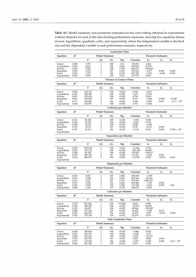
The detailed model summary and parameter estimates for the curve fitting obtainedfor each of the nine flocking performance measures, using six functions (linear, inverse, loga-rithmic, quadratic, cubic, and exponential), where the independent variable is the flock sizeand the dependent variable is each performance measure, respectively. The model summaryand parameter estimates related to experiments without obstacles are provided in Table A5,while Table A6 shows model summary and parameter estimates related to experimentswith obstacles. The values b1, b2, and b3 represent the regression parameters. For example,a quadratic function will be dependantVar = const + (b1 × f lockSize) + (b2 × f lockSize2).The p-value significance (Sig.) reflects whether the relationships observed in the dataare statistically significant. The standard significance level of α = 0.05 is used. If thep-value < α, then the sample provides enough evidence to reject the null hypothesis; thus,changes in the flock size are associated with changes in the performance measure at thepopulation level. The F-value is related to R2 and is an indicator of the overall significancethrough comparing the obtained model against a model that does not contain the flocksize (the intercept model). It is used only when the p-value supports rejecting the nullhypothesis. The null hypothesis for the F-test states that the model with no flock size fitsthe data as well as the model provided. The degrees of freedom d f1 and d f2 are used toobtain the critical value for the F-test. If the F-value is larger than the critical value, then theassociated null hypothesis is rejected, meaning that the data provides enough evidence thatthe model fits the data better than the intercept-only model. When the dependent variable(performance measure) contains a zero value, the exponential model cannot be calculatedfor this variable.

Appl. Sci. 2022, 12, 3630 25 of 29

Table A5. Model summary and parameter estimates for the curve fitting obtained in experimentswithout obstacles for each of the nine flocking performance measures, showing five equations (linear,inverse, logarithmic, quadratic, cubic, and exponential), where the independent variable is the flocksize and the dependent variable is each performance measure, respectively.

Localization Time

Equation R2 Model Summary Parameter Estimates

F d f1 d f2 Sig Constant b1 b2 b3

Linear 0.008 1.551 1 198 0.21 596.80 1.064Logarithmic 0.003 0.621 1 198 0.432 549.036 27.878Inverse 0.000 0.092 1 198 0.762 663.673 −284.653Quadratic 0.018 1.819 2 197 0.165 703.633 −4.277 0.049 0.049Cubic 0.019 1.257 3 196 0.290 657.206 −0.160 −0.041 0.001Exponential 0.032 6.595 1 198 0.011 517.037 0.003

Distance to Center of Mass



Linear 0.404 134.127 1 198 <0.001 5.766 −0.011Logarithmic 0.601 298.740 1 198 <0.001 7.239 −0.541Inverse 0.697 455.018 1 198 <0.001 4.724 15.401Quadratic 0.661 192.028 2 197 <0.001 6.511 −0.048 <0.000 <0.000Cubic 0.711 160.586 3 196 <0.001 7.040 −0.095 0.001 −6.17× 106

Exponential 0.426 146.981 1 198 <0.001 5.733 −0.002

Collisions per Member



Linear 0.221 56.250 1 198 <0.001 −0.185 0.006Logarithmic 0.140 32.215 1 198 <0.001 −0.603 0.195Inverse 0.069 14.672 1 198 <0.001 0.248 −3.628Quadratic 0.315 45.34 2 197 <0.001 0.152 −0.011 0.000Cubic 0.337 33.213 3 196 <0.001 −0.110 0.012 0.000 3.054 × 106

Exponential

Separations per Member



Linear 0.650 368.184 1 198 <0.001 −71.942 2.758Logarithmic 0.452 163.134 1 198 <0.001 −282.284 94.948Inverse 0.246 64.762 1 198 <0.001 134.062 −1854.17Quadratic 0.795 382.765 2 197 <0.001 41.334 −2.906 0.051Cubic 0.814 286.573 3 196 <0.001 −24.798 2.960 −0.076 0.001Exponential

Alignments per Member



Linear 0.015 3.001 1 197 0.085 692.039 −1.389Logarithmic 0.015 2.954 1 197 0.087 832.665 −56.934Inverse 0.013 2.507 1 197 0.115 574.867 1388.522Quadratic 0.015 1.498 2 196 0.226 699.440 −1.760 0.003Cubic 0.015 0.999 3 195 0.394 713.458 −3.003 0.030 0.00Exponential 0.008 1.660 1 197 0.199 604.031 −0.001

Cohesions per Member



Linear 0.725 521.941 1 198 <0.0001 8.625 0.802Logarithmic 0.536 228.370 1 198 <0.001 −55.871 28.490Inverse 0.322 94.027 1 198 <0.001 69.866 −583.987Quadratic 0.840 517.244 2 197 <0.001 36.426 −0.588 0.013Cubic 0.872 443.766 3 196 <0.001 12.919 1.497 −0.033 0.000Exponential 0.782 710.318 1 198 <0.001 20.278 0.015

Task Completion Time



Linear 0.649 365.944 1 198 <0.001 −0.466 0.043Logarithmic 0.527 220.253 1 198 <0.001 −4.238 1.615Inverse 0.340 102.141 1 198 <0.001 2.928 −34.333Quadratic 0.674 203.970 2 197 <0.001 0.282 0.006 0.000Cubic 0.677 136.692 3 196 <0.001 −0.077 0.038 0.000 4.19 × 106

Exponential 0.802 801.140 1 198 <0.001 0.275 0.029

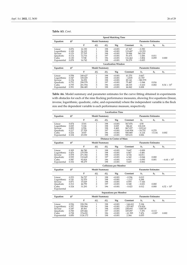
Appl. Sci. 2022, 12, 3630 26 of 29

Table A5. Cont.

Speed Matching Time



Linear 0.076 16.190 1 198 <0.001 67.367 −0.390Logarithmic 0.109 24.192 1 198 <0.001 119.687 −19.353Inverse 0.123 27.703 1 198 <0.001 29.984 543.230Quadratic 0.114 12.716 2 197 <0.001 91.675 −1.606 0.011Cubic 0.130 9.748 3 196 <0.001 116.462 −3.804 0.059 0.000Exponential 0.078 16.742 1 198 <0.001 50.279 −0.005

Localization Window



Linear 0.558 249.627 1 198 <0.001 41.270 0.667Logarithmic 0.347 105.029 1 198 <0.001 −4.835 21.707Inverse 0.154 36.052 1 198 <0.001 89.141 −382.579Quadratic 0.752 298.578 2 197 <0.001 75.487 −1.044 0.016Cubic 0.755 201.554 3 196 <0.001 68.335 −0.410 0.002 8.34 × 105

Exponential 0.591 286.485 1 198 <0.001 46.842 0.008

Table A6. Model summary and parameter estimates for the curve fitting obtained in experimentswith obstacles for each of the nine flocking performance measures, showing five equations (linear,inverse, logarithmic, quadratic, cubic, and exponential) where the independent variable is the flocksize and the dependent variable is each performance measure, respectively.

Localization Time



Linear 0.074 15.81 1 198 <0.001 567.876 4.90Logarithmic 0.025 5.126 1 198 0.025 386.60 118.218Inverse 0.003 0.526 1 198 0.469 867.027 −1012.61Quadratic 0.217 27.329 2 197 <0.001 1160.904 −24.752 0.270Cubic 0.224 18.87 3 196 <0.001 950.885 −6.124 −0.134 0.002Exponential 0.104 23.030 1 198 <0.001 529.631 0.006

Distance to Center of Mass



Linear 0.305 86.780 1 198 <0.001 5.647 −0.009Logarithmic 0.476 179.559 1 198 <0.001 6.967 −0.481Inverse 0.578 271.302 1 198 <0.001 4.724 14.011Quadratic 0.529 110.645 2 197 <0.001 6.342 −0.044 0.000Cubic 0.587 92.824 3 196 <0.001 6.911 −0.095 0.001 −6.64× 106

Exponential 0.332 98.279 1 198 <0.001 5.605 −0.002

Collisions per Member



Linear 0.223 56.737 1 198 <0.001 −0.296 0.012Logarithmic 0.141 32.570 1 198 <0.001 −1.117 0.384Inverse 0.071 15.029 1 198 <0.001 0.555 −7.166Quadratic 0.312 44.759 2 197 <0.001 0.348 −0.021 0.000Cubic 0.324 31.293 3 196 <0.001 −0.023 0.012 0.000 4.32 × 106

Exponential

Separations per Member



Linear 0.536 228.356 1 198 <0.001 −144.410 5.184Logarithmic 0.357 109.964 1 198 <0.001 −525.907 174.826Inverse 0.187 45.561 1 198 <0.001 238.693 −3345.39Quadratic 0.700 229.466 2 197 <0.001 105.097 −7.291 0.113Cubic 0.728 174.652 3 196 <0.001 −61.395 7.476 −0.207 0.002Exponential 0.850 1124.172 1 198 <0.001 2.364 0.055

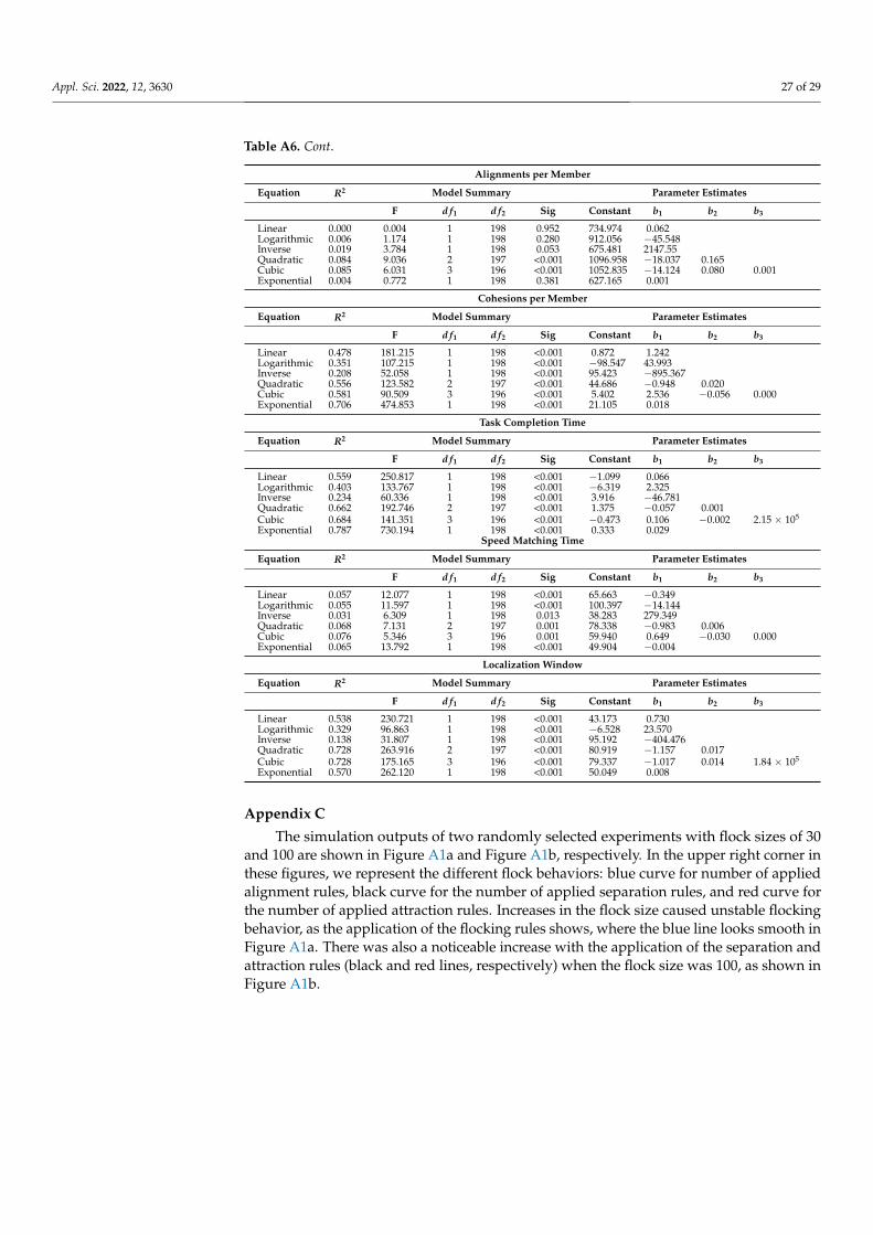
Appl. Sci. 2022, 12, 3630 27 of 29

Table A6. Cont.

Alignments per Member



Linear 0.000 0.004 1 198 0.952 734.974 0.062Logarithmic 0.006 1.174 1 198 0.280 912.056 −45.548Inverse 0.019 3.784 1 198 0.053 675.481 2147.55Quadratic 0.084 9.036 2 197 <0.001 1096.958 −18.037 0.165Cubic 0.085 6.031 3 196 <0.001 1052.835 −14.124 0.080 0.001Exponential 0.004 0.772 1 198 0.381 627.165 0.001

Cohesions per Member



Linear 0.478 181.215 1 198 <0.001 0.872 1.242Logarithmic 0.351 107.215 1 198 <0.001 −98.547 43.993Inverse 0.208 52.058 1 198 <0.001 95.423 −895.367Quadratic 0.556 123.582 2 197 <0.001 44.686 −0.948 0.020Cubic 0.581 90.509 3 196 <0.001 5.402 2.536 −0.056 0.000Exponential 0.706 474.853 1 198 <0.001 21.105 0.018

Task Completion Time



Linear 0.559 250.817 1 198 <0.001 −1.099 0.066Logarithmic 0.403 133.767 1 198 <0.001 −6.319 2.325Inverse 0.234 60.336 1 198 <0.001 3.916 −46.781Quadratic 0.662 192.746 2 197 <0.001 1.375 −0.057 0.001Cubic 0.684 141.351 3 196 <0.001 −0.473 0.106 −0.002 2.15 × 105

Exponential 0.787 730.194 1 198 <0.001 0.333 0.029Speed Matching Time



Linear 0.057 12.077 1 198 <0.001 65.663 −0.349Logarithmic 0.055 11.597 1 198 <0.001 100.397 −14.144Inverse 0.031 6.309 1 198 0.013 38.283 279.349Quadratic 0.068 7.131 2 197 0.001 78.338 −0.983 0.006Cubic 0.076 5.346 3 196 0.001 59.940 0.649 −0.030 0.000Exponential 0.065 13.792 1 198 <0.001 49.904 −0.004

Localization Window



Linear 0.538 230.721 1 198 <0.001 43.173 0.730Logarithmic 0.329 96.863 1 198 <0.001 −6.528 23.570Inverse 0.138 31.807 1 198 <0.001 95.192 −404.476Quadratic 0.728 263.916 2 197 <0.001 80.919 −1.157 0.017Cubic 0.728 175.165 3 196 <0.001 79.337 −1.017 0.014 1.84 × 105

Exponential 0.570 262.120 1 198 <0.001 50.049 0.008

Appendix C

The simulation outputs of two randomly selected experiments with flock sizes of 30and 100 are shown in Figure A1a and Figure A1b, respectively. In the upper right corner inthese figures, we represent the different flock behaviors: blue curve for number of appliedalignment rules, black curve for the number of applied separation rules, and red curve forthe number of applied attraction rules. Increases in the flock size caused unstable flockingbehavior, as the application of the flocking rules shows, where the blue line looks smooth inFigure A1a. There was also a noticeable increase with the application of the separation andattraction rules (black and red lines, respectively) when the flock size was 100, as shown inFigure A1b.

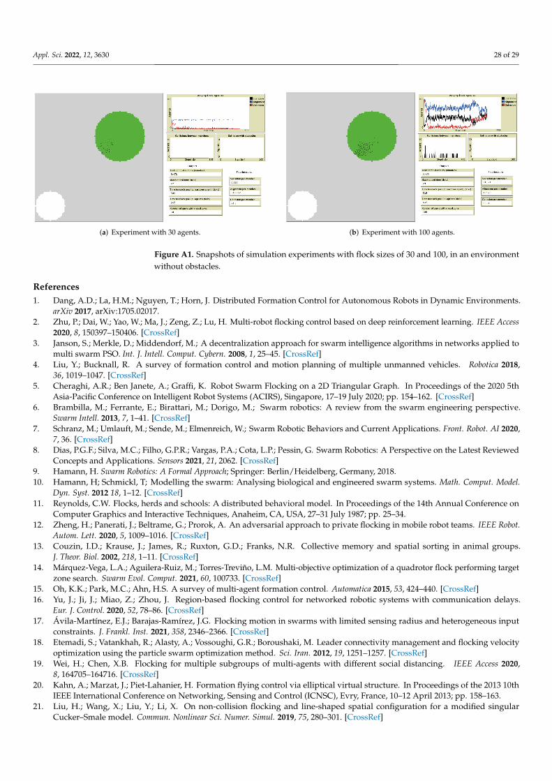
Appl. Sci. 2022, 12, 3630 28 of 29

(a) Experiment with 30 agents. (b) Experiment with 100 agents.

Figure A1. Snapshots of simulation experiments with flock sizes of 30 and 100, in an environmentwithout obstacles.

References1. Dang, A.D.; La, H.M.; Nguyen, T.; Horn, J. Distributed Formation Control for Autonomous Robots in Dynamic Environments.

arXiv 2017, arXiv:1705.02017.2. Zhu, P.; Dai, W.; Yao, W.; Ma, J.; Zeng, Z.; Lu, H. Multi-robot flocking control based on deep reinforcement learning. IEEE Access

2020, 8, 150397–150406. [CrossRef]3. Janson, S.; Merkle, D.; Middendorf, M.; A decentralization approach for swarm intelligence algorithms in networks applied to

multi swarm PSO. Int. J. Intell. Comput. Cybern. 2008, 1, 25–45. [CrossRef]4. Liu, Y.; Bucknall, R. A survey of formation control and motion planning of multiple unmanned vehicles. Robotica 2018,

36, 1019–1047. [CrossRef]5. Cheraghi, A.R.; Ben Janete, A.; Graffi, K. Robot Swarm Flocking on a 2D Triangular Graph. In Proceedings of the 2020 5th

Asia-Pacific Conference on Intelligent Robot Systems (ACIRS), Singapore, 17–19 July 2020; pp. 154–162. [CrossRef]6. Brambilla, M.; Ferrante, E.; Birattari, M.; Dorigo, M.; Swarm robotics: A review from the swarm engineering perspective.

Swarm Intell. 2013, 7, 1–41. [CrossRef]7. Schranz, M.; Umlauft, M.; Sende, M.; Elmenreich, W.; Swarm Robotic Behaviors and Current Applications. Front. Robot. AI 2020,

7, 36. [CrossRef]8. Dias, P.G.F.; Silva, M.C.; Filho, G.P.R.; Vargas, P.A.; Cota, L.P.; Pessin, G. Swarm Robotics: A Perspective on the Latest Reviewed

Concepts and Applications. Sensors 2021, 21, 2062. [CrossRef]9. Hamann, H. Swarm Robotics: A Formal Approach; Springer: Berlin/Heidelberg, Germany, 2018.10. Hamann, H; Schmickl, T; Modelling the swarm: Analysing biological and engineered swarm systems. Math. Comput. Model.

Dyn. Syst. 2012 18, 1–12. [CrossRef]11. Reynolds, C.W. Flocks, herds and schools: A distributed behavioral model. In Proceedings of the 14th Annual Conference on

Computer Graphics and Interactive Techniques, Anaheim, CA, USA, 27–31 July 1987; pp. 25–34.12. Zheng, H.; Panerati, J.; Beltrame, G.; Prorok, A. An adversarial approach to private flocking in mobile robot teams. IEEE Robot.

Autom. Lett. 2020, 5, 1009–1016. [CrossRef]13. Couzin, I.D.; Krause, J.; James, R.; Ruxton, G.D.; Franks, N.R. Collective memory and spatial sorting in animal groups.

J. Theor. Biol. 2002, 218, 1–11. [CrossRef]14. Márquez-Vega, L.A.; Aguilera-Ruiz, M.; Torres-Treviño, L.M. Multi-objective optimization of a quadrotor flock performing target

zone search. Swarm Evol. Comput. 2021, 60, 100733. [CrossRef]15. Oh, K.K.; Park, M.C.; Ahn, H.S. A survey of multi-agent formation control. Automatica 2015, 53, 424–440. [CrossRef]16. Yu, J.; Ji, J.; Miao, Z.; Zhou, J. Region-based flocking control for networked robotic systems with communication delays.

Eur. J. Control. 2020, 52, 78–86. [CrossRef]17. Ávila-Martínez, E.J.; Barajas-Ramírez, J.G. Flocking motion in swarms with limited sensing radius and heterogeneous input

constraints. J. Frankl. Inst. 2021, 358, 2346–2366. [CrossRef]18. Etemadi, S.; Vatankhah, R.; Alasty, A.; Vossoughi, G.R.; Boroushaki, M. Leader connectivity management and flocking velocity

optimization using the particle swarm optimization method. Sci. Iran. 2012, 19, 1251–1257. [CrossRef]19. Wei, H.; Chen, X.B. Flocking for multiple subgroups of multi-agents with different social distancing. IEEE Access 2020,

8, 164705–164716. [CrossRef]20. Kahn, A.; Marzat, J.; Piet-Lahanier, H. Formation flying control via elliptical virtual structure. In Proceedings of the 2013 10th

IEEE International Conference on Networking, Sensing and Control (ICNSC), Evry, France, 10–12 April 2013; pp. 158–163.21. Liu, H.; Wang, X.; Liu, Y.; Li, X. On non-collision flocking and line-shaped spatial configuration for a modified singular

Cucker–Smale model. Commun. Nonlinear Sci. Numer. Simul. 2019, 75, 280–301. [CrossRef]

http://doi.org/10.1109/ACCESS.2020.3016951

http://dx.doi.org/10.1108/17563780810857112

http://dx.doi.org/10.1017/S0263574718000218

http://dx.doi.org/10.1109/ACIRS49895.2020.9162599

http://dx.doi.org/10.1007/s11721-012-0075-2

http://dx.doi.org/10.3389/frobt.2020.00036

http://dx.doi.org/10.3390/s21062062

http://dx.doi.org/10.1080/13873954.2011.601426

http://dx.doi.org/10.1109/LRA.2020.2967331

http://dx.doi.org/10.1006/jtbi.2002.3065

http://dx.doi.org/10.1016/j.swevo.2020.100733

http://dx.doi.org/10.1016/j.automatica.2014.10.022

http://dx.doi.org/10.1016/j.ejcon.2019.08.005

http://dx.doi.org/10.1016/j.jfranklin.2021.01.022

http://dx.doi.org/10.1016/j.scient.2012.06.029

http://dx.doi.org/10.1109/ACCESS.2020.3022395

http://dx.doi.org/10.1016/j.cnsns.2019.04.006

Appl. Sci. 2022, 12, 3630 29 of 29

22. Cao, Y.U.; Kahng, A.B.; Fukunaga, A.S. Cooperative mobile robotics: Antecedents and directions. In Robot Colonies; Springer:Berlin/Heidelberg, Germany, 1997; pp. 7–27.

23. Olfati-Saber, R. Flocking for multi-agent dynamic systems: Algorithms and theory. IEEE Trans. Autom. Control 2006, 51, 401–420.[CrossRef]

24. Semnani, S.H.; Basir, O.A. Semi-flocking algorithm for motion control of mobile sensors in large-scale surveillance systems.IEEE Trans. Cybern. 2014, 45, 129–137. [CrossRef]

25. Khrustalev, M.M. Synthesis of adaptive control strategies for flocks of mobile robots using Aristotle’s mechanics.IFAC-PapersOnLine 2018, 51, 525–529. [CrossRef]

26. Zhang, H.; Nie, P.; Sun, Y.; Shi, Y. Fixed-time flocking problem of a Cucker–Smale type self-propelled particle model. J. Frankl. Inst.2020, 357, 7054–7068. [CrossRef]

27. Krause, J.; Ruxton, G.D.; Ruxton, G.; Ruxton, I.G. Living in Groups; Oxford University Press: New York, NY, USA, 2002.28. Caro, T. Antipredator Defenses in Birds and Mammals; University of Chicago Press: Chicago, IL, USA, 2005.29. McSweeney, P.L.; McNamara, J.P. Encyclopedia of Dairy Sciences, 3rd ed.; Academic Press: Cambridge, MA, USA, 2021.30. Cresswell, W.; Quinn, J.L. Predicting the optimal prey group size from predator hunting behaviour. J. Anim. Ecol. 2011,

80, 310–319. [CrossRef] [PubMed]31. Vine, I. Detection of prey flocks by predators. J. Theor. Biol. 1973, 40, 207–210. [CrossRef]32. Hintz, W.D.; Lonzarich, D.G. Maximizing foraging success: The roles of group size, predation risk, competition, and ontogeny.

Ecosphere 2018, 9, 10. [CrossRef]33. Rakic, K.; Rosic, M.; Boljat, I. A Survey of Agent-Based Modelling and Simulation Tools for Educational Purpose. Tehnicki Vjesnik

2020, 27, 1014–1020.34. Abar, S.; Theodoropoulos, G.K.; Lemarinier, P.; O’Hare, G.M. Agent Based Modelling and Simulation tools: A review of the

state-of-art software. Comput. Sci. Rev. 2017, 24, 13–33. [CrossRef]35. Tisue, S.; Wilensky, U. NetLogo: Design and implementation of a multi-agent modeling environment. In Proceedings of Agent;

Springer: Cham, Switzerland, 2004; Volume 2004, pp. 7–9.36. Pallant, J. SPSS Survival Manual: A Step by Step Guide to Data Analysis Using IBM SPSS; Routledge: Oxfordshire, UK, 2020.37. Johnson, R.A.; Wichern, D.W. Applied Multivariate Statistical Analysis; Pearson: London, UK, 2014; Volume 6.38. Cohen, J. Statistical Power Analysis for the Behavioral Sciences; Routledge: Oxfordshire, UK, 2013.39. Guest, P.G. Numerical Methods of Curve Fitting; Cambridge University Press: Cambridge, NY, USA, 2012.40. Smith, K.; Fry, P.; Shannon, P.; Groebner, D. Business Statistics: A Decision-making Approach. J.-Oper. Res. Soc. 2005, 56, 1347.

http://dx.doi.org/10.1109/TAC.2005.864190

http://dx.doi.org/10.1109/TCYB.2014.2328659

http://dx.doi.org/10.1016/j.ifacol.2018.11.475

http://dx.doi.org/10.1016/j.jfranklin.2020.05.012

http://dx.doi.org/10.1111/j.1365-2656.2010.01775.x

http://www.ncbi.nlm.nih.gov/pubmed/21244418

http://dx.doi.org/10.1016/0022-5193(73)90127-6

http://dx.doi.org/10.1002/ecs2.2456

http://dx.doi.org/10.1016/j.cosrev.2017.03.001

Effect of Formation Size on Flocking Formation Performance ...

Documents