Flocking algorithm for autonomous flying robots - arXiv

Flocking algorithm for autonomous flying robots 1

Flocking algorithm for autonomous flying robots

Csaba Virágh1, Gábor Vásárhelyi

1,2, Norbert Tarcai

1, Tamás Szörényi

1, Gergő Somorjai

1,2, Tamás

Nepusz1,2

, Tamás Vicsek1,2

1 ELTE Department of Biological Physics, 1117 Budapest, Pázmány Péter Sétány 1/A

2 MTA-ELTE Statistical and Biological Physics Research Group, 1117 Budapest, Pázmány Péter

Sétány 1/A

E-mail of corresponding author: [email protected]

Abstract. Animal swarms displaying a variety of typical flocking patterns would not exist without

underlying safe, optimal and stable dynamics of the individuals. The emergence of these universal

patterns can be efficiently reconstructed with agent-based models. If we want to reproduce these

patterns with artificial systems, such as autonomous aerial robots, agent-based models can also be

used in the control algorithm of the robots. However, finding the proper algorithms and thus

understanding the essential characteristics of the emergent collective behaviour of robots requires the

thorough and realistic modeling of the robot and the environment as well. In this paper, first, we

present an abstract mathematical model of an autonomous flying robot. The model takes into account

several realistic features, such as time delay and locality of the communication, inaccuracy of the on-

board sensors and inertial effects. We present two decentralized control algorithms. One is based on a

simple self-propelled flocking model of animal collective motion, the other is a collective target

tracking algorithm. Both algorithms contain a viscous friction-like term, which aligns the velocities of

neighbouring agents parallel to each other. We show that this term can be essential for reducing the

inherent instabilities of such a noisy and delayed realistic system. We discuss simulation results about

the stability of the control algorithms, and perform real experiments to show the applicability of the

algorithms on a group of autonomous quadcopters. Bio-inspiration works in our case two-ways. On

the one hand, the whole idea of trying to build and control a swarm of robots comes from the

observation that birds tend to flock to optimize their behaviour as a group. On the other hand, by using

a realistic simulation framework and studying the group behaviour of autonomous robots we can learn

about the major factors influencing the flights of bird flocks.

1. Introduction

Collective motion is an impressive phenomenon, that can be observed in a wide range of biological

systems, such as fish schools, bird flocks, herds of mammals or migrating cells [1]. These systems produce

the same universal feature: the velocity vectors of neighbouring individuals tend to become parallel to each

other. This behaviour and the underlying control mechanism seem to be a prerequisite of safe, stable and

collision-free motion. Therefore, it might be advantageous to incorporate the mathematical models that

reproduce group flight patterns into the control of artificial systems, a group of autonomous flying robots, for

example. By autonomous we mean that every agent uses on-board sensors to measure its state and performs

all controlling calculations with an on-board computer, i.e., the control system is decentralized. This

definition prohibits central processing of the group dynamics by an external computer, but allows the use of

e.g. on-board GPS devices for external reference of position. Our study is valid for any kind of object that is


capable of moving in arbitrary directions independently of its orientation, within a reasonable velocity range

(including zero velocity hovering). Typical flying robots that satisfy this criteria are the so-called quadro-,

hexa-, and octocopters, commonly named as multicopters.

According to Reynolds, collective motion of various kinds of entities can be interpreted as a

consequence of three simple principles [2]: repulsion in short range to avoid collisions, a local interaction

called alignment rule to align the velocity vectors of nearby units and preferably global positional constraint

to keep the flock together. These rules can be interpreted in mathematical form as an agent-based model, i.e.,

a (discrete or continuous) dynamical system that describes the time-evolution of the velocities of each unit

individually.

The simplest agent-based models of flocking describe the alignment rule as an explicit mathematical

axiom: every unit aligns its velocity vector towards the average velocity vector of the units in its

neighbourhood (including itself) [3]. It is possible to generalize this term by adding coupling of accelerations

[4], preferred directions [5] and adaptive decision-making schemes to extend the stability for higher

velocities [6]. In other (more specific) models, the alignment rule is a consequence of interaction forces [7]

or velocity terms based on over-damped dynamics [8].

An important feature of the alignment rule terms in flocking models is their locality; units align their

velocity towards the average velocity of other units within limited range only. In flocks of autonomous

robots, the communication between the robots usually also have a finite range. In other words, the units can

send messages (e.g. their positions and velocities) only to nearby other units. Another analogy between

nature based flocking models and autonomous robotic systems is that both can be considered as based on

agents, i.e., autonomous units subject to some system-specific rules. In the flocking models, the velocity

vectors of the agents evolve individually through a dynamical system. In a group of autonomous flying

robots, every robot has its own on-board computer and on-board sensors, thus the control of the dynamics is

individual-based, decentralized.

Because of these similarities, some of the principles of animal flocking models can be integrated into

the control dynamics of autonomous robots [9]. For example, Turgut et al. presented a dynamical system

based on the simplest flocking model and used it to control the motion of so-called Kobots in two

dimensions, on the ground [10]. In three dimensions, Hauert et al. presented experiments with fixed-wing

agents, as a simple application of two of the three rules postulated by Reynolds (note that there was no true

repulsion between the units, they flew at different altitudes) [11].

Thus the principles of flocking models presented above are useful for creating control algorithms for

autonomous robots. However, we shall not underestimate the ability of animals to maintain highly coherent

motion. The prerequisites of smooth collective motion include robustness against reaction times and possible

delay in the communication, noisy sensory inputs or unpredictable environmental disturbances, like wind.

Animals seem to overcome these difficulties efficiently. However, in robotic systems, these effects can cause

unpredictable effects on stability. It is well known, for example that if time delay is present in the

communication between swarming agents, instabilities can emerge [12].

One of the main goals of this paper is to provide a model of a general autonomous flying robot

integrated into a realistic simulation framework. This model can be used to study the stability of flocking

algorithms from the perspective of the deficiencies of realistic systems. The model should contain as many

system-specific features as we can take into account, but also should be applicable for many kinds of robots.

Due to this „duality” we define the axioms of the robot model with several independent parameters,

corresponding to each source of deficiency in the realistic framework. Specific experimental situations can

be realized with a fine-tuned set of these parameters.

Another goal of this paper is to demonstrate that some features of animal flocking models can be

useful in collective robotics only if some specific extra aspects of the robots are taken into account. We show

that the principles of flocking behaviour can be transformed into unique components of the dynamical

system implemented as the control framework of robots. A short-range repulsion is needed to avoid

collisions and an implicit viscous friction-like alignment rule term is efficiently used for damping the


amplitude of oscillations caused by the imperfections of the system. With simulations and experiments on

autonomous quadcopters, we study the stability of two realistic bio-inspired situations: i) a general self-

propelled flocking scenario inside a bounded area and ii) a collective target tracking setup to reach and

smoothly stop at a predefined position.

2. Realistic model of a flying robot

In this section, we present a model of a flying robot based on some features that are general in many

realistic robotic systems. In such systems, the motion of the robots is controlled by a low-level algorithm,

e.g. a velocity-based PID controller (see Appendix A). This low-level control algorithm typically has an

input, the desired velocity vector of the actual robot. During flock flights, the time-dependence of the desired

velocity of the ith unit can be a function of the positions ( ix ) and velocities ( iv ) of the other units:

))}({,)}(({)( 11

d N

jj

N

jjii tt=t vxfv ,

where N is the number of agents and the if function contains the arbitrary features of the controlling

dynamics. In ideal case, the velocity of the ith robot changes to )(d tiv at time t immediately. However, a

robotic system is never ideal; some of its deficiencies shall be modelled:

1. Inertia – The robots cannot change their attitude or velocity immediately. In general, the desired

velocity is an input of a low-level controller algorithm. We assume that in an optimal setup, the

system can reach the desired velocity with exponential convergence, with a characteristic time

CTRLτ . A simple controller algorithm satisfying this behaviour is a PID controller (see Appendix

A). The magnitude of acceleration is also limited to maxa .

2. Inner noise – We have to take into account the inaccuracy of the sensors that provide relative

position and velocity information. For example, the uncertainty of the position and velocity

measured by a GPS device can be modelled as a stochastic function )(s tiη (see Appendix B).

This function can be characterized by a standard deviation sσ . Note that the term „inner noise”

can refer to the inaccuracy of any kind of sensors used in actual robot system.

3. Refresh rate of the sensors – Refresh rate of sensory inputs fundamentally defines the reaction

time and agility of robots. We consider a limited refresh rate of the sensors: every unit updates

sensory data with frequency 1st . In our current model, 1

st is constant.

4. Locality of the communication – The communication between the units have a finite range, cr ,

thus if the distance between two units is greater than cr , they cannot interact with each other. In

other words: the if function depends on jx only if c<|| rij xx .

5. Time delay – By the time a unit receives and processes position and velocity data from another

unit, data will be old due to data processing and transmission delays. In the simplest approach,

time delay can be considered as a constant value, delt .

6. General noise – A delta-correlated (Gaussian) outer noise term )(tiη with standard deviation

σ is added to the acceleration of the units. This term is a model of unpredictable environmental

effects such as fluctuations in the wind compensation of the low-level control algorithm.

Considering all the points above, our definition of a realistic system is the equivalent of defining the

set })}(),({,,,,,{ 1s

sdelcmaxCTRLNjjj ttttraτ ηη . Time delay and communication range are hard to measure, can

change randomly and have the most dangerous effects on stability. Therefore any kind of if has to be

investigated with various delt and cr values.

The final form of the model is an equation that defines the acceleration ( )(tia ) of each unit:

max

CTRL

sd

sd

sd

,)()()(

min|)()()(|

)()()(+)(=)( a

τ

ttt

ttt

ttttt iii

iii

iiiii

vvv

vvv

vvvηa , (1)


))(+)(,)}(+)({),(+(t),)}(+)(({=)( s

del

s

del

s

del

s

del

d tttttttttttt iiijjjiiijjjii vvvvxxxxfv ,

where )(si tx and )(s

i tv give a measure of the integrated position and velocity noise for a random variable

)(s tiη , which results from solving the second-order stochastic differential equation )()()( sss ttt iii ηvx . In

the expression of if , ij{...} denotes a set with iterator ij . The function if depends on the actual position

and velocity of the ith agent and the delayed position and velocity of the other agents and only changes

with 1st frequency. The equations above can be solved using the Euler and Euler-Maruyama methods.

In the rest of the paper, we choose specific if functions with two main features:

1. if depends only on relative coordinates of the interacting units, i.e., no global positional

information is needed in the system:

))(+)(,)}(+)({,)}()(+(t))(({= s

del

s

del

s

del

s

del ttttttttttt iiijjjijijijii vvvvxxxxff .

2. interaction terms in if can be expressed as a sum of local pairwise interactions ( ijf ) with other

units:

|)~~|( )~,~,~~(= c

1=

jijiij

N

j

iji rθ xxvvxxff ,

where )(xθ defines the communication range explicitely; it equals to 0 if 0<x and equals to 1 if 0x .

ix~ and iv~ are the measured position and velocity values including the modelled inner noise term: s+=~iii xxx and

s+=~iii vvv .

We also choose fixed values for some of the parameters: s 0.2=st , s 1=CTRLτ , 2max m/s 6=a ,

22s /sm 0.005=σ . These values represent our state-of-the-art experimental setup with quadcopters. For

practical reasons, we saturate the magnitude of desired velocities expressed by the if functions at

m/s 4=maxv .

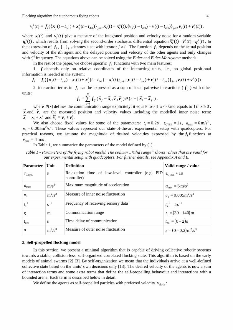
In Table 1, we summarize the parameters of the model defined by (1).

Table 1 - Parameters of the flying robot model. The column „Valid range” shows values that are valid for

our experimental setup with quadcopters. For further details, see Appendix A and B.

Parameter Unit Definition Valid range / value

CTRLτ s Relaxation time of low-level controller (e.g. PID

controller) s 1CTRL τ

maxa 2m/s Maximum magnitude of acceleration 2max m/s 6=a

sσ 22/sm Measure of inner noise fluctuation 22s /sm 0.005=σ

1st 1s Frequency of receiving sensory data 11

s s 5= t

cr m Communication range m 14030=c r

delt s Time delay of communication s 20=del t

σ 32/sm Measure of outer noise fluctuation 32/sm 0.20= σ

3. Self-propelled flocking model

In this section, we present a minimal algorithm that is capable of driving collective robotic systems

towards a stable, collision-less, self-organized correlated flocking state. This algorithm is based on the early

models of animal swarms [2] [3]. By self-organization we mean that the individuals arrive at a well-defined

collective state based on the units’ own decisions only [13]. The desired velocity of the agents is now a sum

of interaction terms and some extra terms that define the self-propelling behavoiur and interactions with a

bounded arena. Each term is described below in detail.

We define the agents as self-propelled particles with preferred velocity flockv :


||= flock

SPP

i

ii v

v

vv . (2)

3.1. Short-range repulsion

To avoid collisions, we define a local linear repulsion between the units:

)||(||

)||(= 0

0rep

ijij

ij

ij

ij rθrD

ddd

dv

, (3)

where ijij xxd = , D is the strength of the repulsion, 0r is the interaction range. We consider that the

amplitude of fluctuations in the measured position caused by inner noise can be in the same range as 0r . In

such a noisy system, the simple linear repulsion is superior to higher-order terms, because errors in the

measured position do not cause sudden changes or singularities in the output. If the robots were able to

measure their positions more accurately, higher-order terms, like the Lennard-Jones potential could be used

[14].

3.2. Velocity alignment of neighbours

Any kind of velocity alignment rule term in realistic control algorithms should satisfy three

assumptions: it should i) relax the velocity difference of units close to each other; ii) be local and iii) have an

upper threshold value even when the distance between the units are close-to-zero (similar with the repulsion

term). In the light of these, we implement the alignment rule with a viscous friction-like interaction term,

similarly to [15] and [16]:

2min

frictfrict

)|}|,max{(=

ij

ij

ijr

Cd

vvv

, (4)

where frictC is the strength of the alignment and minr defines a threshold to avoid division by close-to-

zero distances.

This term is a specific, practical choice for taking into account the tendency of the particles/robots to

align their direction of motion. In some sense it is a discrete counterpart of the viscous friction term which

would be present in a continuum description such as, e.g., the one considered first by Toner and Tu [17].

The locality of the viscous friction term in practice is guaranteed by the inverse-square decay of the

term as a function of distance. However, the maximal velocity maxv and the value of frictC also has to be

bounded. The interaction becomes local if the magnitude offrictijv gets negligible compared to || SPP

iv at large

distances, i.e. when max

2

flockfrict /2|| vvC ijd for large values of || ijd . The optimal ratio of flockv and

frictC is thus defined by the limit of the velocities and the desired interaction range.

3.3. Boundaries and shill agents

An important principle of flocking behaviour is some kind of global positional constraint that

contributes to the integrity of the flock. In simulation, this feature of the positional constraint can be well

substituted by using periodic boundary conditions. This is an effective method for examining the large-scale

statistical properties of the system. In real experiments, periodic boundary conditions can be imitated by

closing the units into a quasi-low-dimensional space, e.g. into a ring-shaped arena [18] [19], but in three

dimensions these restrictions are not practical at all.

To study the flocking model with simulations, we placed the units into a square-shaped arena with

repulsive walls. We define the repulsion of the wall as virtual „shill” agents [20]. If the units are outside the

wall, those shill agents try to align the velocities of the units towards the centre of the arena:


i

i

iiii vd v

xx

xxxxxxv

|| )R),,,(R

~|,(| sC=

a

aflockaashill

shill , (5)

where shillC is the strength of the „shill-repulsion”, ax is the position of the centre of the arena,

)( s d R, x, is a sigmoid curve which smoothly reduces the strength of the repulsion inside the arena:

dRx

dRRxRxd

Rx

dRx

+>if 1

+,if1+2

ππsin

0,if 0

=),,( s . (6)

R~

is a function that defines the shape of the arena (in this case, a square with side length R ).

Note that the walls of the arena are pre-defined globally in the simulation, but the repulsive term only

depends on the relative coordinates axx i , thus in real robotic systems the arena can be sensed locally, the

same way as neighbouring units are.

The sum of the three terms defined above are the minimal prerequisites of flocking behaviour, in other

words, with these terms we could guarantee stable and collision-free collective motion in our simulations and

experiments:

)( )+(+= c

frictrepshillSPPd

ij

ij

ijijiii rθ dvvvvv

. (7)

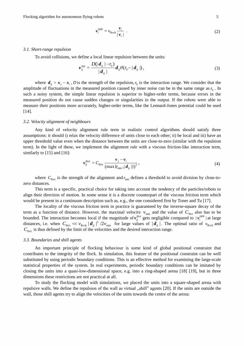
In Table 2, we summarize the parameters of the self-propelled flocking algorithm.

Table 2 - Parameters of the self-propelled flocking algorithm

Parameter Unit Definition

flockv m/s Preferred „flocking” velocity

D 1/s Strength of repulsion

0r m Interaction range of repulsion

frictC 2m Strength of viscous friction

minr m This parameter defines a threshold to avoid division by zero

R m Side length of the square-shaped arena

shillC Maximum strength of shill-repulsion near walls

d m Characteristic „width” of the wall

4. Collective target tracking

In this section, we demonstrate that the interaction terms repijv and frict

ijv can be included in other, task-

specific control algorithms. We have created a collective target tracking algorithm using an a priori defined

fixed target point. The algorithm allows the units to perform a smooth transition between two stable states:

the flocking state (far from the target) and the collective hovering state (around the target). During this

transition near the target point, the preferred magnitude of the velocity has to approach zero smoothly and the

coherence and robustness of the flock should be maintained without signs of jamming or oscillations.

Imagine the flock as a „meta-agent” at the centre of mass moving towards the target position with

desired velocity 0v . Each unit must accomplish two tasks without collisions: i) approach this meta-agent

close enough for joining the flock and ii) move parallel with the meta-agent for reaching the target


collectively.

According to our definition, communication between the robots is local. Therefore, calculating the

global centre of mass is physically not possible. Nevertheless, robots can calculate a local centre of mass

(CoM), based on the information available from within their communication range (in a sphere-shaped

environment with radius cr ). Attraction towards the target point is thus defined as:

|| ),|,(| s+

|| ),|,(| s=

CoMtrg

CoMtrg

trg

CoMtrg

CoM

CoM

CoM

CoM

0

trg

i

ii

ii

iiiii drdrv

xx

xxxx

xx

xxxxv , (8)

where 0v is the magnitude of the preferred velocity, trgx is the position of the target, CoM

ix is the

position of the local centre of mass from the viewpoint of the ith agent, trgr is the radius of the target area,

CoMr is the radius of the sphere-shaped meta-agent. )( s d R, x, is the sigmoid function defined in (6). Note

that the locality of the viscous friction term defined in (4) depends on the values of 0v and frictC in this

algorithm. Also note that different weights for the target and CoM tracking terms could also be introduced,

but we keep these weights at 1 now to keep the algorithm as simple as possible.

The magnitude of the target tracking term saturates at 0v :

|}|,{min||

=~ trg0trg

trgtrg

i

i

ii v v

v

vv . (9)

The final desired velocity calculated by the algorithm is:

)( )+(+~= cfrictreptrgd

ijij

ijijii rθ dvvvv

. (10)

In Table 3, we summarize the parameters of the target tracking algorithm.

Table 3: Parameters of the target tracking algorithm

Parameter Unit Definition

v0 m/s Preferred velocity far from the target position

CoMr m Radius of expected flock size (characteristic size of the meta-agent)

trgr m Characteristic size of the target area

d m Charascteristic size of the „transition” area – velocity of the meta-

agent approach to zero near the target point with this „relaxation

length”.

5., Results and discussion

In this section, we present realistic simulation and robotic experiment results.

5.1. Simulation of the flocking algorithm

First of all, we demonstrate that typical flocking patterns can emerge even with large delays in the

communication and with the presence of inner and outer noise. The coherence of the flocking state can be

indicated with the order parameter

N

i ij ji

ji

tt

tt

NNt

1=scal

|)(||)(|

)()(

1

1=)(ψ

vv

vv, (11)

where N is the number of agents, )()( tt ji vv is the scalar product of two velocity vectors. In ideal

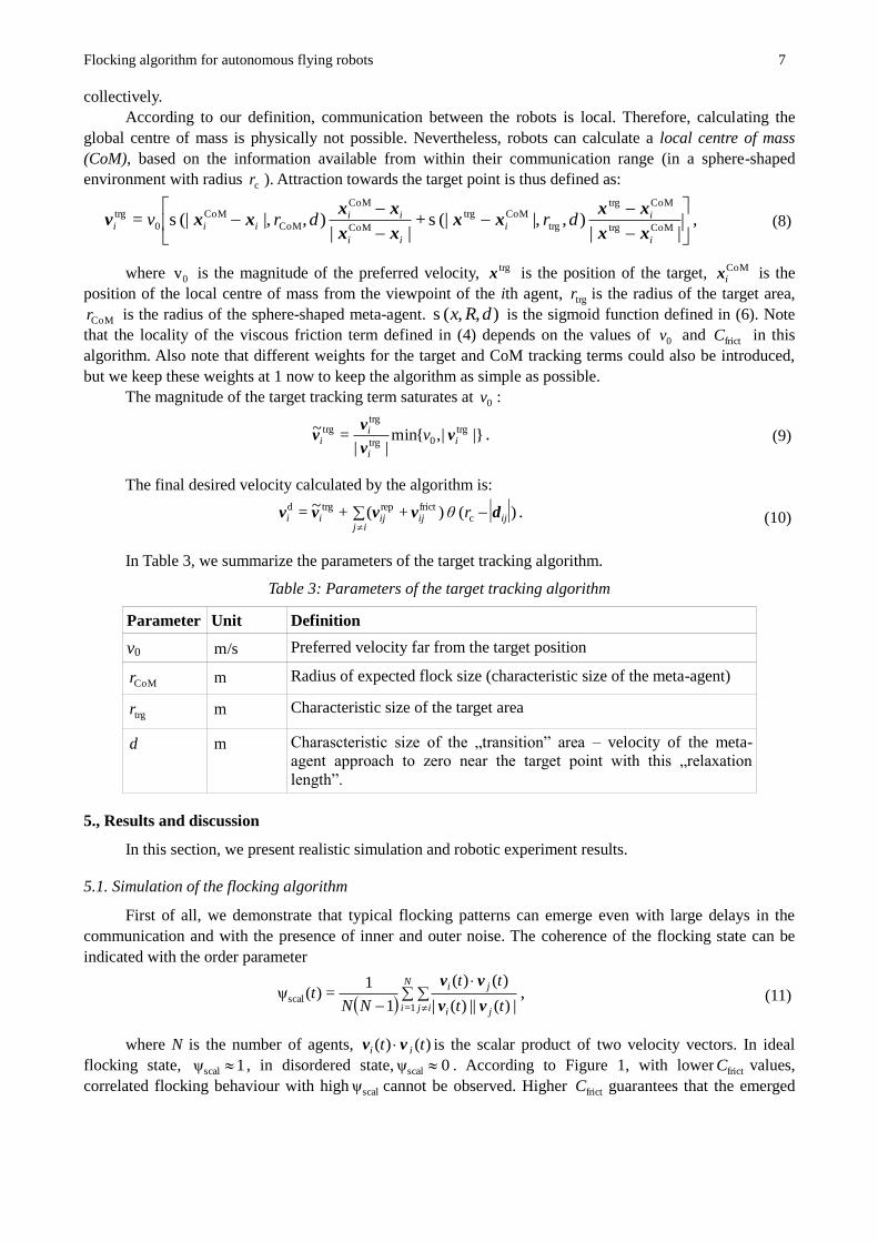
flocking state, 1ψscal , in disordered state, 0ψscal . According to Figure 1, with lower frictC values,

correlated flocking behaviour with high scalψ cannot be observed. Higher frictC guarantees that the emerged


flocking states are stable even in the presence of noise and large time delay.

5.2. Simulation of the target tracking algorithm

The goal of this subsection is to show that the stability of the target tracking algorithm can be

guaranteed with our selection of interaction terms used in the flocking algorithm. To study the stability, we

analyze two possible quasi-stable states of the system: the flocking state (large velocity, far from the target

position) and the hovering state (zero velocity, near the target position). Note that our goal is to show the

effects of the interaction terms on the stability, therefore the other parameters ( 0v , CoMr , trgr and d ) were set

to fixed default values. Parameter choice was optimized to guarantee the stable completion of the target

tracking task with smooth transition between the flocking and hovering states in an ideal case.

To initialize the flocking state, the units are placed within a 35 m wide square-shaped area 100 m away

from the target point. After starting the simulated experiment, in ideal case, the velocity vectors of the units

should become parallel and should have the same magnitude, i.e., stable, ordered flocking behaviour should

be observed with 1ψscal . We define the end of the flocking state when all units are at most CoM2r far from

the target point. After this point, scalψ shall not be used as an order parameter due to the decreased

velocities around the target.

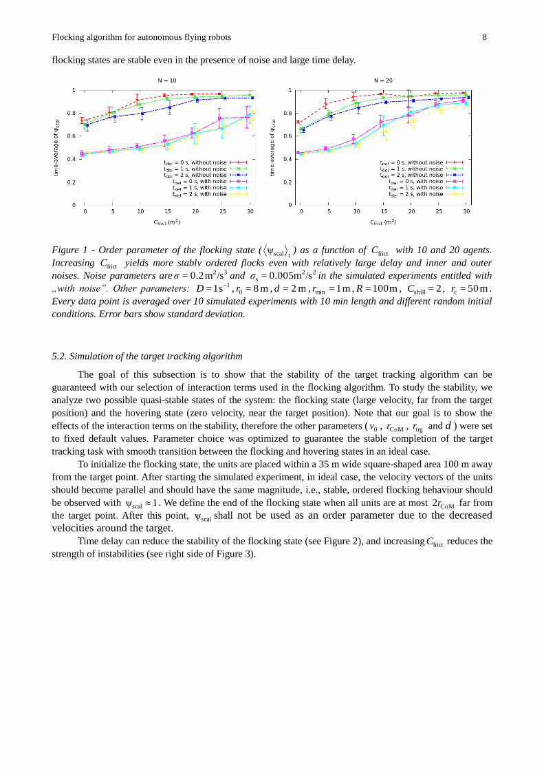
Time delay can reduce the stability of the flocking state (see Figure 2), and increasing frictC reduces the

strength of instabilities (see right side of Figure 3).

Figure 1 - Order parameter of the flocking state (tscalψ ) as a function of frictC with 10 and 20 agents.

Increasing frictC yields more stably ordered flocks even with relatively large delay and inner and outer

noises. Noise parameters are 32/sm 0.2=σ and 22s /sm 0.005=σ in the simulated experiments entitled with

„with noise”. Other parameters: 1s 1= D , m 8=0r , m 2=d , m 1=minr , m 100=R , 2=shillC , m 50=cr .

Every data point is averaged over 10 simulated experiments with 10 min length and different random initial

conditions. Error bars show standard deviation.


To initialize the hovering state, units are placed around the target point inside a circle with radius

trgr and with zero initial velocity. Due to the interaction forces and the attraction towards the target point, in

ideal case, the units will arrange themselves into a lattice-like structure, where the distance between

neighbours is approximately 0r . However, if time delay is present in the system, dangerous oscillations can

emerge. Since that kind of instability can lead to collisions, it has to be eliminated. The strength of the

instability in the hovering state can be described by the average velocity-magnitude:

N

ji t

Nt

1=vel |)(|

1=)(ψ v . (12)

Increase of )(ψvel t represents growing amplitude and/or frequency of the oscillations.

In the hovering state, the strength of the delay-induced oscillations can be reduced with higher frictC

and smaller D values either with or without inner and outer noises (see left side of Figure 3). It is important

to note that the instabilities can be reduced by an optimal setup of the interaction parameters only if the

sphere around the local centre of mass with radius CoMr is large enough to contain all units with at least the

repulsive interaction range ( 0r ) apart from each other. With giving the units enough space around the target,

we can reduce all superfluous excitations caused by the repulsive interactions.

According to Figure 3, the additive Gaussian noise term can also reduce the instabilities caused by the

time delay in the hovering state. This is a general feature of coupled delayed dynamical systems, since

random noise usually acts against synchrony and resonance.

Figure 2 - Trajectories of 10 agents with and without viscous friction, without noise, with s 1=delt . The

arrows represent the actual velocity vector of a unit. Insets show the order parameter scalψ versus time. The

square represents the starting area; the circle is the environment around the target point with radius

m 15.15=CoMr . Without the friction-like term, oscillations can emerge during the flocking behaviour, what

causes severe quasi-stochastic fluctuations in )(ψscal t . Other parameters: 1s 1= D , m 8=0r ,

m 6.5=trgr , m 2=d , m/s 2=0v , m 100=cr .


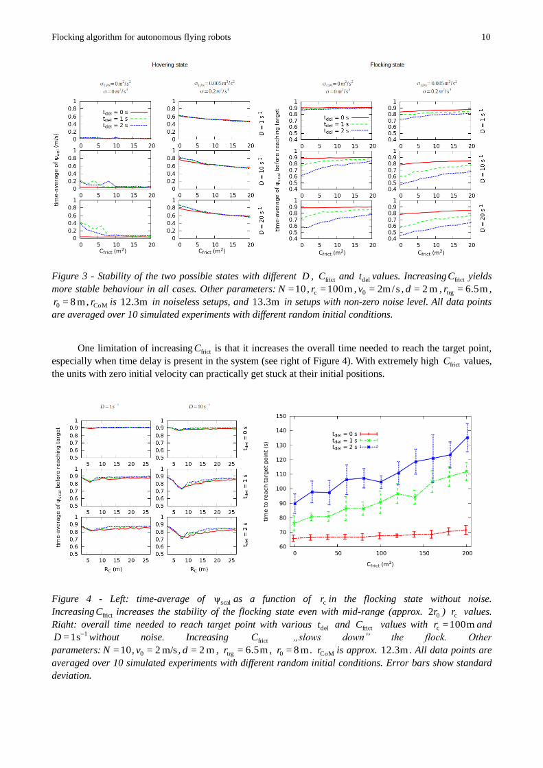
One limitation of increasing frictC is that it increases the overall time needed to reach the target point,

especially when time delay is present in the system (see right of Figure 4). With extremely high frictC values,

the units with zero initial velocity can practically get stuck at their initial positions.

Figure 4 - Left: time-average of scalψ as a function of cr in the flocking state without noise.

Increasing frictC increases the stability of the flocking state even with mid-range (approx. 02r ) cr values.

Right: overall time needed to reach target point with various delt and frictC values with m 100=cr and 1s 1= D without noise. Increasing frictC „slows down” the flock. Other

parameters: 10=N , m/s 2=0v , m 2=d , m 6.5=trgr , m 8=0r . CoMr is approx. m 12.3 . All data points are

averaged over 10 simulated experiments with different random initial conditions. Error bars show standard

deviation.

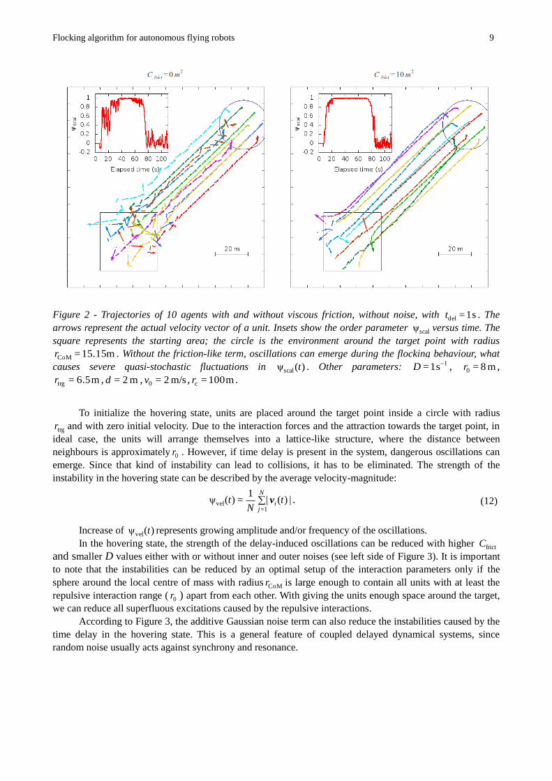
Figure 3 - Stability of the two possible states with different D , frictC and delt values. Increasing frictC yields

more stable behaviour in all cases. Other parameters: 10=N , m 100=cr , s/m2=0v , m 2=d , m 6.5=trgr ,

m 8=0r , CoMr is m 12.3 in noiseless setups, and m 13.3 in setups with non-zero noise level. All data points

are averaged over 10 simulated experiments with different random initial conditions.


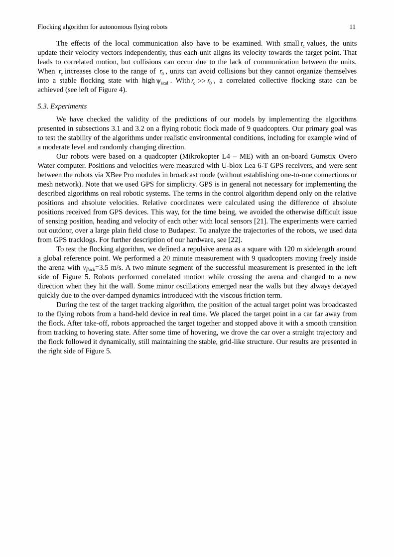
The effects of the local communication also have to be examined. With small cr values, the units

update their velocity vectors independently, thus each unit aligns its velocity towards the target point. That

leads to correlated motion, but collisions can occur due to the lack of communication between the units.

When cr increases close to the range of 0r , units can avoid collisions but they cannot organize themselves

into a stable flocking state with high scalψ . With 0c rr , a correlated collective flocking state can be

achieved (see left of Figure 4).

5.3. Experiments

We have checked the validity of the predictions of our models by implementing the algorithms

presented in subsections 3.1 and 3.2 on a flying robotic flock made of 9 quadcopters. Our primary goal was

to test the stability of the algorithms under realistic environmental conditions, including for example wind of

a moderate level and randomly changing direction.

Our robots were based on a quadcopter (Mikrokopter L4 – ME) with an on-board Gumstix Overo

Water computer. Positions and velocities were measured with U-blox Lea 6-T GPS receivers, and were sent

between the robots via XBee Pro modules in broadcast mode (without establishing one-to-one connections or

mesh network). Note that we used GPS for simplicity. GPS is in general not necessary for implementing the

described algorithms on real robotic systems. The terms in the control algorithm depend only on the relative

positions and absolute velocities. Relative coordinates were calculated using the difference of absolute

positions received from GPS devices. This way, for the time being, we avoided the otherwise difficult issue

of sensing position, heading and velocity of each other with local sensors [21]. The experiments were carried

out outdoor, over a large plain field close to Budapest. To analyze the trajectories of the robots, we used data

from GPS tracklogs. For further description of our hardware, see [22].

To test the flocking algorithm, we defined a repulsive arena as a square with 120 m sidelength around

a global reference point. We performed a 20 minute measurement with 9 quadcopters moving freely inside

the arena with vflock=3.5 m/s. A two minute segment of the successful measurement is presented in the left

side of Figure 5. Robots performed correlated motion while crossing the arena and changed to a new

direction when they hit the wall. Some minor oscillations emerged near the walls but they always decayed

quickly due to the over-damped dynamics introduced with the viscous friction term.

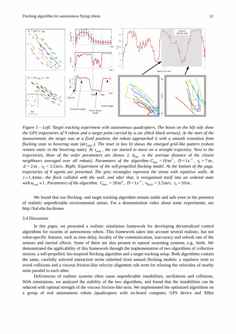
During the test of the target tracking algorithm, the position of the actual target point was broadcasted

to the flying robots from a hand-held device in real time. We placed the target point in a car far away from

the flock. After take-off, robots approached the target together and stopped above it with a smooth transition

from tracking to hovering state. After some time of hovering, we drove the car over a straight trajectory and

the flock followed it dynamically, still maintaining the stable, grid-like structure. Our results are presented in

the right side of Figure 5.


We found that our flocking- and target tracking algorithm remain stable and safe even in the presence

of realistic unpredictable environmental noises. For a demonstration video about some experiments, see

http://hal.elte.hu/drones

5.4 Discussion

In this paper, we presented a realistic simulation framework for developing decentralized control

algorithms for swarms of autonomous robots. This framework takes into account several realistic, but not

robot-specific features, such as time delay, locality of the communication, inaccuracy and refresh rate of the

sensors and inertial effects. Some of these are also present in natural swarming systems, e.g., birds. We

demonstrated the applicability of this framework through the implementation of two algorithms of collective

motion: a self-propelled, bio-inspired flocking algorithm and a target tracking setup. Both algorithms contain

the same, carefully selected interaction terms inherited from natural flocking models: a repulsive term to

avoid collisions and a viscous friction-like velocity alignment rule term for relaxing the velocities of nearby

units parallel to each other.

Deficiencies of realistic systems often cause unpredictable instabilities, oscillations and collisions.

With simulations, we analyzed the stability of the two algorithms, and found that the instabilities can be

reduced with optimal strength of the viscous friction-like term. We implemented the optimized algorithms on

a group of real autonomous robots (quadcopters with on-board computer, GPS device and XBee

Figure 5 – Left: Target tracking experiment with autonomous quadcopters. The boxes on the left side show

the GPS trajectories of 9 robots and a target point carried by a car (thick black arrows). At the start of the

measurement, the target was at a fixed position, the robots approached it with a smooth transition from

flocking state to hovering state (at a)/b)t ). The inset in box b) shows the emerged grid-like pattern (robots

remain static in the hovering state). At startt , the car started to move on a straight trajectory. Next to the

trajectories, three of the order parameters are shown. ( minr is the average distance of the closest

neighbours averaged over all robots). Parameters of the algorithm: 2frict m 10=C , 1s 1= D , m 7=0r ,

m 2=d , m/s 3.5=0v . Right: Experiment of the self-propelled flocking model. At the bottom of the page,

trajectories of 8 agents are presented. The grey rectangles represent the arena with repulsive walls. At

min 1.4 t , the flock collided with the wall, and after that, it reorganized itself into an ordered state

with 1ψscal . Parameters of the algorithm: 2frict m 20=C , 1s 1= D , m/s 3.5=flockv , m 10=0r .


communication module). Successful experiments represent a direct proof of the applicability of the model

and the algorithms and also show the stability of the algorithms when the system is exposed to unpredictable

environmental noises.

Our realistic model can be enhanced in many ways. One big issue is synchronism vs asynchronism in

the model and in reality, which appears at many levels: in the update of the simulation iterations, in the

modelled delay or in the communication. We have not yet treated these issues explicitly. However, we

always tested the simulation framework with larger delays compared to what was expected in our real system

to overestimate the unwanted effects of the delay. Moreover, general random noise terms were introduced in

order to compensate for the artificial synchrony of the used delay model. In the future we will certainly

enhance our delayed communication model with asynchronous update. In the real experiments synchrony is

not present at any level due to the decentralized control scheme; nevertheless, simulation results and

experimental results are quite similar in general. This fact indicates that even though synchrony is an

important artifact in the simulation framework, its effects are limited in the noisy environment.

In the current setup we used the generally available global positioning system as the most

straightforward way of measuring position, velocity and heading. This way, we could concentrate on the

development of a functional control framework in a real setup and did not have to deal with any form of

“artificial vision” that is yet beyond our current knowledge. However, GPS outages could occur at any time

due to several independent reasons. In the current model, GPS outages are not modelled explicitely, only

through the finite sensor update rates and with the delay in the communication. In case of long periods

without sensory inputs the system cannot function, per se. On the other hand, any real application requires

robust behaviour. It will be an essential improvement to get around this problem when future systems

become able to rely on truly local sensory information. In three dimensions this is yet an unsolved issue;

however, we already designed our algorithms to be based on only local data to provide a framework for

further, fully autonomous development.

Bio-inspiration was one of the main motivations of our work. Studying the analogies and differences

between the behaviour of swarming robotic systems and flocking phenomena in nature reveals many

important messages, some of which serve as reverse-bio-inspiration for biological research. For example, we

are now inspired to search for additional factors allowing the very highly coherent motion of pigeon flocks,

since our experiments suggests that a very short reaction time itself cannot account for the perfectly

synchronized flight of many kinds of birds.

Acknowledgement

This work was supported by the FP7 ERC COLLMOT grant. No. 227878., G. V. was partly supported by EU

TÁMOP 4.2.4.A/1-11-1-2012-0001

Appendix A: PID Controller

To model the specific features of a velocity-based PID controller, we performed measurements with

real autonomous flying robots (Mikrokopter L4 – ME R/C-controllable quadcopters with a self-developed

autopilot board based on a Gumstix Overo Water minicomputer). The low-level controller algorithm

implemented on the on-board computer has two inputs: desired (or „target”) velocity and measured velocity.

The output of that controller is a control signal value fed to the standard main board of the quadrocopter. The

PID loop for controlling velocity is based on the following equation:

bias0

idpout '+)d'(+d

)(d+)(=)( φtteK

t

teKteKtφ

t

, (13)

where )(te is the error signal, the difference of the desired and the measured velocity:

)()(=)( md tvtvte ( v can be the north-south or the east-west component of the velocity vector), the

pK , iK , dK values are the parameters of the proportional, integral and differential terms and dbias = ζvφ is


a feed-forward bias term determined by the linear approximation of the measured velocity as a function of

the control signal. We have analyzed the logged data of our robot experiments for finding the proper

parameters. The real velocity of the robot is a function of )(out tφ (See right side of Figure 6).

The time-evolution of the real velocity depends on the pK , iK and dK parameters. In ideal case, an

exponential convergence can be observed with characteristic time CTRLτ . In non-ideal case, the behaviour is

either over-damped with larger settling time or under-damped with oscillations.

Appendix B: GPS device – example for modelling inner noise

By inner noise we mean the uncertainty of the positions and velocities measured by sensors on the

robots. In the case of our quadcopters, the position data is provided by U-blox Lea 6-T GPS receivers. We

have made a model to reproduce two main features of the inaccuracy of this device: i) distribution of the

velocity measurement error is close to Gaussian, and ii) measured position accuracy is 2.5 m (50% CEP).

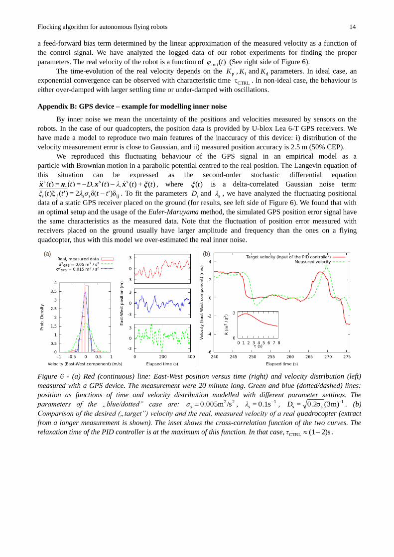
We reproduced this fluctuating behaviour of the GPS signal in an empirical model as a

particle with Brownian motion in a parabolic potential centred to the real position. The Langevin equation of

this situation can be expressed as the second-order stochastic differential equation

)(+)()(=)(=)( ss

sss

s ttλtDtt ξxxηx , where )(tξ is a delta-correlated Gaussian noise term:

ijss )δ'δ(2=)'()ξ( ttσλttξ ji . To fit the parameters sD and sλ , we have analyzed the fluctuating positional

data of a static GPS receiver placed on the ground (for results, see left side of Figure 6). We found that with

an optimal setup and the usage of the Euler-Maruyama method, the simulated GPS position error signal have

the same characteristics as the measured data. Note that the fluctuation of position error measured with

receivers placed on the ground usually have larger amplitude and frequency than the ones on a flying

quadcopter, thus with this model we over-estimated the real inner noise.

Figure 6 - (a) Red (continuous) line: East-West position versus time (right) and velocity distribution (left)

measured with a GPS device. The measurement were 20 minute long. Green and blue (dotted/dashed) lines:

position as functions of time and velocity distribution modelled with different parameter settings. The

parameters of the „blue/dotted” case are: 22s /sm 0.005σ , 1

s s 0.1= λ , 1ss (3m)0.2σ= D . (b)

Comparison of the desired („target”) velocity and the real, measured velocity of a real quadrocopter (extract

from a longer measurement is shown). The inset shows the cross-correlation function of the two curves. The

relaxation time of the PID controller is at the maximum of this function. In that case, s)2(1CTRL τ .


References

[1] T. Vicsek and A. Zafeiris, “Collective motion,” Physics Reports, vol. 517, no. 3-4, pp. 71 – 140,

2012

[2] C.W. Reynolds, 1987 „Flocks, herds and schools: A distributed behavioural model.” SIGGRAPH

Comput. Graph, 21, 25-34, 1987

[3] T. Vicsek, A. Czirók, E. Ben-Jacob, I. Cohen, and O. Shochet, “Novel type of phase transition in a

system of self-driven particles,” Phys. Rev. Lett. vol. 75, no. 6, pp. 1226–1229, 1995

[4] P. Szabó, M. Nagy, and T. Vicsek, “Transitions in a self-propelled-particles model with coupling of

accelerations,” Phys. Rev. E, vol. 79, no. 2, p. 021908, Feb 2009

[5] J. Krause, N. R. Franks, S. A. Levin, and I. D. Couzin, “Effective leadership and decision-making in

animal groups on the move,” Nature, vol. 433, pp. 513–516, 2004

[6] H. Dong, Y. Zhao, and S. Gao, “A fuzzy-rule-based couzin model,” Journal of Control Theory and

Applications, vol. 11, no. 2, pp. 311–315, 2013

[7] D. Grossman, I. S. Aranson, and E. B. Jacob, “Emergence of agent swarm migration and vortex

formation through inelastic collisions,” New Journal of Physics, vol. 10, no. 2, p. 023036, 2008

[8] B. Szabó, G. J. Szőllősi, B. Gönci, Zs, D. Selmeczi, and T. Vicsek, “Phase transition in the collective

migration of tissue cells: Experiment and model,” Physical Review E, vol. 74, no. 6, pp.

061908+, Dec. 2006

[9] M. Brambilla, E. Ferrante, M. Birattari, and M. Dorigo, “Swarm robotics: A review from the swarm

engineering perspective,” Swarm Intelligence, vol. 7, pp. 1–41, 2013

[10] A. Turgut, H. Çelikkanat, F. Gökçe, and E. Şahin, “Self-organized flocking in mobile robot swarms,”

Swarm Intelligence, vol. 2, pp. 97–120, 2008, 10.1007/s11721-008-0016-2

[11] S. Hauert, S. Leven, M. Varga, F. Ruini, A. Cangelosi, J.-C. Zufferey, and D. Floreano, “Reynolds

flocking in reality with fixed-wing robots: Communication range vs. maximum turning rate,” in

Intelligent Robots and Systems (IROS), 2011 IEEE/RSJ International Conference on, 2011, pp.

5015–5020

[12] E. Forgoston and I. B. Schwartz, “Delay-induced instabilities in self-propelling swarms,” Phys. Rev.

E, vol. 77, p. 035203, Mar 2008

[13] Floreano, D., & Mattiussi, C., “Bio-inspired artificial intelligence: theories, methods, and

technologies”, MIT press, Section 7.1, pp. 516, 2008

[14] E. Ferrante, A. E. Turgut, C. Huepe, A. Stranieri, C. Pinciroli, and M. Dorigo, “Self-organized

flocking with a mobile robot swarm: a novel motion control method.” Adaptive Behaviour, vol.

20, no. 6, pp. 460–477, 2012

[15] F. Cucker and S. Smale, „Emergent behavior in flocks.” IEEE Transactions on Automatic Control,

852-862, 2007

[16] D. Helbing, I. Farkas, and T. Vicsek, „Simulating dynamical features of escape panic,” Nature, 407,

487-490, 2000

[17] J. Toner and Y. Tu, “Long-range order in a two-dimensional dynamical XY model: How birds fly

together,” Phys. Rev. Lett., vol. 75, pp. 4326–4329, Dec 1995

[18] C. A. Yates, R. Erban, C. Escudero, I. D. Couzin, J. Buhl, I. G. Kevrekidis, P. K. Maini, and D. J. T.

Sumpter, “Inherent noise can facilitate coherence in collective swarm motion,” Proceedings of

the National Academy of Sciences, vol. 106, no. 14, pp. 5464–5469, Apr. 2009

[19] N. Tarcai, Cs. Virágh, D. Ábel, M. Nagy, P. L. Várkonyi, G. Vásárhelyi, and T. Vicsek, “Patterns,

transitions and the role of leaders in the collective dynamics of a simple robotic flock,” Journal

of Statistical Mechanics: Theory and Experiment, vol. 2011, no. 04, p. P04010, 2011

[20] J. Han, M. Li, and L. Guo, „Soft control on collective behavior of a group of autonomous agents by a

shill agent,” Journal of Systems Science and Complexity, 19, 54-62, 2006

[21] C. Moeslinger, T. Schmickl, and K. Crailsheim, „A Minimalist Flocking Algorithm for Swarm

Robots.” In: Kampis, G., Karsai, I., and Szathmáry, E. (Ed.), Advances in Artificial Life. Darwin

Meets von Neumann, Springer Berlin Heidelberg, 2011

[22] G. Vásárhelyi, Cs. Virágh, N. Tarcai, T. Szörényi, G. Somorjai, T. Nepusz, and T. Vicsek, „Outdoor

flocking and formation flight with autonomous aerial robots.” submitted to IROS 2014, 2014

Flocking algorithm for autonomous flying robots - arXiv

Documents