Efficient Inner-product Algorithm for Stabilizer States H´ ector J. Garc´ ıa * Igor L. Markov * Andrew W. Cross † [email protected] [email protected] [email protected] * University of Michigan – EECS Department 2260 Hayward Street, Ann Arbor, MI, 48109-2121 † IBM T. J. Watson Research Center Yorktown Heights, NY 10598 Abstract Large-scale quantum computation is likely to require massive quantum error correction (QEC). QEC codes and circuits are described via the stabilizer formalism, which represents stabilizer states by keeping track of the operators that preserve them. Such states are obtained by stabilizer circuits (consisting of CNOT, Hadamard and Phase only) and can be represented compactly on conventional computers using Ω(n 2 ) bits, where n is the number of qubits [10]. Although techniques for the efficient simulation of stabilizer circuits have been studied extensively [1], [9], [10], techniques for efficient manipulation of stabilizer states are not currently available. To this end, we leverage the theoretical insights from [1] and [16] to design new algorithms for: (i) obtaining canonical generators for stabilizer states, (ii) obtaining canonical stabilizer circuits, and (iii) computing the inner product between stabilizer states. Our inner-product algorithm takes O(n 3 ) time in general, but observes quadratic behavior for many practical instances relevant to QECC (e.g., GHZ states). We prove that each n-qubit stabilizer state has exactly 4(2 n - 1) nearest-neighbor stabilizer states, and verify this claim experimentally using our algorithms. We design techniques for representing arbitrary quantum states using stabilizer frames and generalize our algorithms to compute the inner product between two such frames. I. I NTRODUCTION Gottesman [9] and Knill showed that for certain types of non-trivial quantum circuits known as stabilizer circuits, efficient simulation on classical computers is possible. Stabilizer circuits are exclusively composed of stabilizer gates – Controlled-NOT, Hadamard and Phase gates (Figure 1a) – followed by measurements in the computational basis. Such circuits are applied to a computational basis state (usually |00...0i) and produce output states called stabilizer states. The case of purely unitary stabilizer circuits (without measurement gates) is considered often, e.g., by consolidating measurements at the end. Stabilizer circuits can be simulated in poly-time by keeping track of a set Pauli operators that stabilize 1 the quantum state. Such stabilizer operators uniquely represent a stabilizer state up to an unobservable global phase. Equation 1 shows that the number of n-qubit stabilizer states grows as 2 n 2 /2 , therefore, describing a generic stabilizer state requires at least n 2 /2 bits. Despite their compact representation, stabilizer states can exhibit multi-qubit entanglement and are often encountered in many quantum information applications such as Bell states, GHZ states, error-correcting codes and one-way quantum computation. To better understand the role stabilizer states play in such applications, researchers have designed techniques to quantify the amount of entanglement [8], [18], [12] in such states and studied relevant properties such as purification schemes [7], Bell inequalities [11] and equivalence classes [17]. Efficient algorithms for the manipulation of stabilizer states (e.g., computing the angle between them), can help lead to additional insights related to linear-algebraic and geometric properties of stabilizer states. In this work, we describe in detail algorithms for the efficient computation of the inner product between stabilizer states. We adopt the approach outlined in [1], which requires the synthesis of a unitary stabilizer circuit that maps a stabilizer state to a computational basis state. The work in [1] shows that, for any unitary stabilizer circuit, there exists an equivalent block- structured canonical circuit that applies a block of Hadamard (H) gates only, followed by a block of CNOT (C) only, then a block of Phase (P ) gates only, and so on in the 7-block sequence H-C-P -C-P -C-H. Using an alternate representation for stabilizer states, the work in [16] proves the existence of a (H-C-P -CZ )-canonical circuit, where the CZ block consists of Controlled-Z (CPHASE) gates. However, no algorithms are known to synthesize such smaller 4-block circuits given an arbitrary stabilizer state. In contrast, we describe an algorithm for synthesizing (H-C-CZ -P -H)-canonical circuits given any input stabilizer state. We prove that any n-qubit stabilizer state |ψi has exactly 4(2 n - 1) nearest-neighbors – stabilizer states |ϕi such that |hψ|ϕi| attains the largest possible value 6=1. Furthermore, we design techniques for representing arbitrary quantum states using stabilizer frames and generalize our algorithms to compute the inner product between two such frames. This paper is structured as follows. Section II reviews the stabilizer formalism and relevant algorithms for manipulating stabilizer-based representations of quantum states. Section III describes our circuit-synthesis and inner-product algorithms. In Section IV, we evaluate the performance of our algorithms. Our findings related to geometric properties of stabilizer states are 1 An operator U is said to stabilize a state iff U |ψi = |ψi. 1 arXiv:1210.6646v3 [cs.ET] 7 Aug 2013

Welcome message from author
This document is posted to help you gain knowledge. Please leave a comment to let me know what you think about it! Share it to your friends and learn new things together.
Transcript

Efficient Inner-product Algorithmfor Stabilizer States
Hector J. Garcıa∗ Igor L. Markov∗ Andrew W. Cross†[email protected] [email protected] [email protected]
∗ University of Michigan – EECS Department2260 Hayward Street, Ann Arbor, MI, 48109-2121
† IBM T. J. Watson Research CenterYorktown Heights, NY 10598
Abstract
Large-scale quantum computation is likely to require massive quantum error correction (QEC). QEC codes and circuits aredescribed via the stabilizer formalism, which represents stabilizer states by keeping track of the operators that preserve them. Suchstates are obtained by stabilizer circuits (consisting of CNOT, Hadamard and Phase only) and can be represented compactly onconventional computers using Ω(n2) bits, where n is the number of qubits [10]. Although techniques for the efficient simulationof stabilizer circuits have been studied extensively [1], [9], [10], techniques for efficient manipulation of stabilizer states are notcurrently available. To this end, we leverage the theoretical insights from [1] and [16] to design new algorithms for: (i) obtainingcanonical generators for stabilizer states, (ii) obtaining canonical stabilizer circuits, and (iii) computing the inner product betweenstabilizer states. Our inner-product algorithm takes O(n3) time in general, but observes quadratic behavior for many practicalinstances relevant to QECC (e.g., GHZ states). We prove that each n-qubit stabilizer state has exactly 4(2n−1) nearest-neighborstabilizer states, and verify this claim experimentally using our algorithms. We design techniques for representing arbitrary quantumstates using stabilizer frames and generalize our algorithms to compute the inner product between two such frames.
I. INTRODUCTION
Gottesman [9] and Knill showed that for certain types of non-trivial quantum circuits known as stabilizer circuits, efficientsimulation on classical computers is possible. Stabilizer circuits are exclusively composed of stabilizer gates – Controlled-NOT,Hadamard and Phase gates (Figure 1a) – followed by measurements in the computational basis. Such circuits are applied toa computational basis state (usually |00...0〉) and produce output states called stabilizer states. The case of purely unitarystabilizer circuits (without measurement gates) is considered often, e.g., by consolidating measurements at the end. Stabilizercircuits can be simulated in poly-time by keeping track of a set Pauli operators that stabilize1 the quantum state. Such stabilizeroperators uniquely represent a stabilizer state up to an unobservable global phase. Equation 1 shows that the number of n-qubitstabilizer states grows as 2n
2/2, therefore, describing a generic stabilizer state requires at least n2/2 bits. Despite their compactrepresentation, stabilizer states can exhibit multi-qubit entanglement and are often encountered in many quantum informationapplications such as Bell states, GHZ states, error-correcting codes and one-way quantum computation. To better understand therole stabilizer states play in such applications, researchers have designed techniques to quantify the amount of entanglement [8],[18], [12] in such states and studied relevant properties such as purification schemes [7], Bell inequalities [11] and equivalenceclasses [17]. Efficient algorithms for the manipulation of stabilizer states (e.g., computing the angle between them), can helplead to additional insights related to linear-algebraic and geometric properties of stabilizer states.
In this work, we describe in detail algorithms for the efficient computation of the inner product between stabilizer states.We adopt the approach outlined in [1], which requires the synthesis of a unitary stabilizer circuit that maps a stabilizer stateto a computational basis state. The work in [1] shows that, for any unitary stabilizer circuit, there exists an equivalent block-structured canonical circuit that applies a block of Hadamard (H) gates only, followed by a block of CNOT (C) only, thena block of Phase (P ) gates only, and so on in the 7-block sequence H-C-P -C-P -C-H . Using an alternate representationfor stabilizer states, the work in [16] proves the existence of a (H-C-P -CZ)-canonical circuit, where the CZ block consistsof Controlled-Z (CPHASE) gates. However, no algorithms are known to synthesize such smaller 4-block circuits given anarbitrary stabilizer state. In contrast, we describe an algorithm for synthesizing (H-C-CZ-P -H)-canonical circuits given anyinput stabilizer state. We prove that any n-qubit stabilizer state |ψ〉 has exactly 4(2n − 1) nearest-neighbors – stabilizer states|ϕ〉 such that |〈ψ|ϕ〉| attains the largest possible value 6= 1. Furthermore, we design techniques for representing arbitraryquantum states using stabilizer frames and generalize our algorithms to compute the inner product between two such frames.
This paper is structured as follows. Section II reviews the stabilizer formalism and relevant algorithms for manipulatingstabilizer-based representations of quantum states. Section III describes our circuit-synthesis and inner-product algorithms. InSection IV, we evaluate the performance of our algorithms. Our findings related to geometric properties of stabilizer states are
1An operator U is said to stabilize a state iff U |ψ〉 = |ψ〉.
1
arX
iv:1
210.
6646
v3 [
cs.E
T]
7 A
ug 2
013

H = 1√2
(1 11 −1
)P =
(1 00 i
)CNOT =
1 0 0 00 1 0 00 0 0 10 0 1 0
X =
(0 11 0
)Y =
(0 −ii 0
)Z =
(1 00 −1
)
Fig. 1. (a) Unitary stabilizer gates Hadamard (H), Phase (P) Fig. 1. (b) The Pauli matrices.and Controlled-NOT (CNOT).
described in Section V. In Section VI, we discuss stabilizer frames and how they can be used to represent arbitrary states andextend our algorithms to compute the inner product between frames. Section VII closes with concluding remarks.
II. BACKGROUND AND PREVIOUS WORK
Gottesman [10] developed a description for quantum states involving the Heisenberg representation often used by physiciststo describe atomic phenomena. In this model, one describes quantum states by keeping track of their symmetries rather thanexplicitly maintaining complex vectors. The symmetries are operators for which these states are 1-eigenvectors. Algebraically,symmetries form group structures, which can be specified compactly by group generators. It turns out that this approach, alsoknown as the stabilizer formalism, can be used to represent an important class of quantum states.
A. The stabilizer formalism
A unitary operator U stabilizes a state |ψ〉 if |ψ〉 is a 1–eigenvector of U , i.e., U |ψ〉 = |ψ〉 [9], [14]. We are interested inoperators U derived from the Pauli matrices shown in Figure 1b The following table lists the one-qubit states stabilized bythe Pauli matrices.
X : (|0〉+ |1〉)/√
2 −X : (|0〉 − |1〉)/√
2
Y : (|0〉+ i |1〉)/√
2 −Y : (|0〉 − i |1〉)/√
2Z : |0〉 −Z : |1〉
Observe that I stabilizes all states and −I does not stabilize any state. As an example, the entangled state (|00〉+ |11〉)/√
2is stabilized by the Pauli operators X⊗X , −Y ⊗Y , Z⊗Z and I⊗ I . As shown in Table I, it turns out that the Pauli matricesalong with I and the multiplicative factors ±1, ±i, form a closed group under matrix multiplication [14]. Formally, the Pauligroup Gn on n qubits consists of the n-fold tensor product of Pauli matrices, P = ikP1⊗· · ·⊗Pn such that Pj ∈ I,X, Y, Zand k ∈ 0, 1, 2, 3. For brevity, the tensor-product symbol is often omitted so that P is denoted by a string of I , X , Y and Zcharacters or Pauli literals and a separate integer value k for the phase ik. This string-integer pair representation allows us tocompute the product of Pauli operators without explicitly computing the tensor products,2 e.g., (−IIXI)(iIY II) = −iIY XI .Since | Gn |= 4n+1, Gn can have at most log2 | Gn |= log2 4n+1 = 2(n+ 1) irredundant generators [14]. The key idea behindthe stabilizer formalism is to represent an n-qubit quantum state |ψ〉 by its stabilizer group S(|ψ〉) – the subgroup of Gn thatstabilizes |ψ〉. As the following theorem shows, if |S(|ψ〉)| = 2n, the group uniquely specifies |ψ〉.
Theorem 1. For an n-qubit pure state |ψ〉 and k ≤ n, S(|ψ〉) ∼= Zk2 . If k = n, |ψ〉 is specified uniquely by S(|ψ〉) and iscalled a stabilizer state.
Proof: (i) To prove that S(|ψ〉) is commutative, let P,Q ∈ S(|ψ〉) such that PQ |ψ〉 = |ψ〉. If P and Q anticommute,−QP |ψ〉 = −Q(P |ψ〉) = −Q |ψ〉 = − |ψ〉 6= |ψ〉. Thus, P and Q cannot both be elements of S(|ψ〉).(ii) To prove that every element of S(|ψ〉) is of degree 2, let P ∈ S(|ψ〉) such that P |ψ〉 = |ψ〉. Observe that P 2 = ilI forl ∈ 0, 1, 2, 3. Since P 2 |ψ〉 = P (P |ψ〉) = P |ψ〉 = |ψ〉, we obtain il = 1 and P 2 = I .(iii) From group theory, a finite Abelian group with a2 = a for every element must be ∼= Zk2 .(iv) We now prove that k ≤ n. First note that each independent generator P ∈ S(|ψ〉) imposes the linear constraint P |ψ〉 = |ψ〉on the 2n-dimensional vector space. The subspace of vectors that satisfy such a constraint has dimension 2n−1, or half the space.Let gen(|ψ〉) be the set of generators for S(|ψ〉). We add independent generators to gen(|ψ〉) one by one and impose their
TABLE IMULTIPLICATION TABLE FOR PAULI MATRICES. SHADED CELLS
INDICATE ANTICOMMUTING PRODUCTS.
I X Y Z
I I X Y ZX X I iZ −iYY Y −iZ I iXZ Z iY −iX I
2This holds true due to the identity: (A⊗ B)(C ⊗D) = (AC ⊗ BD).
2

linear constraints, to limit |ψ〉 to the shared 1-eigenvector. Thus the size of gen(|ψ〉) is at most n. In the case |gen(|ψ〉)| = n,the n independent generators reduce the subspace of possible states to dimension one. Thus, |ψ〉 is uniquely specified.
The proof of Theorem 1 shows that S(|ψ〉) is specified by only log2 2n = n irredundant stabilizer generators. Therefore,an arbitrary n-qubit stabilizer state can be represented by a stabilizer matrix M whose rows represent a set of generatorsg1, . . . , gn for S(|ψ〉). (Hence we use the terms generator set and stabilizer matrix interchangeably.) Since each gi is a stringof n Pauli literals, the size of the matrix is n × n. The phases of each gi are stored separately using a vector of n integers.Therefore, the storage cost for M is Θ(n2), which is an exponential improvement over the O(2n) cost often encountered invector-based representations.
Theorem 1 suggests that Pauli literals can be represented using only two bits, e.g., 00 = I , 01 = Z, 10 = X and 11 = Y .Therefore, a stabilizer matrix can be encoded using an n×2n binary matrix or tableau. The advantage of this approach is thatthis literal-to-bits mapping induces an isomorphism Z2n
2 → Gn because vector addition in Z22 is equivalent to multiplication
of Pauli operators up to a global phase. The tableau implementation of the stabilizer formalism is covered in [1], [14].
Proposition 2. The number of n-qubit pure stabilizer states is given by
N(n) = 2nn−1∏k=0
(2n−k + 1) = 2(.5+o(1))n2
(1)
The proof of Proposition 2 can be found in [1]. An alternate interpretation of Equation 1 is given by the simple recurrencerelation N(n) = 2(2n + 1)N(n− 1) with base case N(1) = 6. For example, for n = 2 the number of stabilizer states is 60,and for n = 3 it is 1080. This recurrence relation stems from the fact that there are 2n + 1 ways of combining the generatorsof N(n− 1) with additional Pauli matrices to form valid n-qubit generators. The factor of 2 accounts for the increase in thenumber of possible sign configurations. Table II and Appendix A list all two-qubit and three-qubit stabilizer states, respectively.
Observation 3. Consider a stabilizer state |ψ〉 represented by a set of generators of its stabilizer group S(|ψ〉). Recall fromthe proof of Theorem 1 that, since S(|ψ〉) ∼= Zn2 , each generator imposes a linear constraint on |ψ〉. Therefore, the set ofgenerators can be viewed as a system of linear equations whose solution yields the 2n basis amplitudes that make up |ψ〉.Thus, one needs to perform Gaussian elimination to obtain the basis amplitudes from a generator set.
Canonical stabilizer matrices. Although stabilizer states are uniquely determined by their stabilizer group, the set of generatorsmay be selected in different ways. For example, the state |ψ〉 = (|00〉+ |11〉)/
√2 is uniquely specified by any of the following
stabilizer matrices:
M1 =XX M2 =
XX M3 =-Y Y
ZZ -Y Y ZZ
One obtains M2 from M1 by left-multiplying the second row by the first. Similarly, one can also obtain M3 from M1 orM2 via row multiplication. Observe that, multiplying any row by itself yields II , which stabilizes |ψ〉. However, II cannot be
TABLE IISIXTY TWO-QUBIT STABILIZER STATES AND THEIR CORRESPONDING PAULI GENERATORS. SHORTHAND
NOTATION REPRESENTS A STABILIZER STATE AS α0, α1, α2, α3 WHERE αi ARE THE NORMALIZED AMPLITUDESOF THE BASIS STATES. THE BASIS STATES ARE EMPHASIZED IN BOLD. THE FIRST COLUMN LISTS STATES WHOSE
GENERATORS DO NOT INCLUDE AN UPFRONT MINUS SIGN, AND OTHER COLUMNS INTRODUCE THE SIGNS. A SIGNCHANGE CREATES AN ORTHOGONAL VECTOR. THEREFORE, EACH ROW OF THE TABLE GIVES AN ORTHOGONAL
BASIS. THE CELLS IN DARK GREY INDICATE STABILIZER STATES WITH FOUR NON-ZERO BASIS AMPLITUDES, I.E.,αi 6= 0 ∀ i. THE ∠ COLUMN INDICATES THE ANGLE BETWEEN THAT STATE AND |00〉, WHICH HAS 12
NEAREST-NEIGHBOR STATES (LIGHT GRAY) AND 15 ORTHOGONAL STATES (⊥).
STATE GEN’TORS ∠ STATE GEN’TORS ∠ STATE GEN’TORS ∠ STATE GEN’TORS ∠
SE
PAR
AB
LE
1, 1, 1, 1 IX, XI π/3 1,−1, 1,−1 -IX, XI π/3 1, 1,−1,−1 IX, -XI π/3 1,−1,−1, 1 -IX, -XI π/31, 1, i, i IX, YI π/3 1,−1, i,−i -IX, YI π/3 1, 1,−i,−i IX, -YI π/3 1,−1,−i, i -IX, -YI π/31, 1, 0, 0 IX, ZI π/4 1,−1, 0, 0 -IX, ZI π/4 0, 0, 1, 1 IX, -ZI ⊥ 0, 0, 1,−1 -IX, -ZI ⊥1, i, 1, i IY, XI π/3 1,−i, 1,−i -IY, XI π/3 1, i,−1,−i IY, -XI π/3 1,−i,−1, i -IY, -XI π/31, i, i,−1 IY, YI π/3 1,−i, i, 1 -IY, YI π/3 1, i,−i, 1 IY, -YI π/3 1,−i,−i,−1 -IY, -YI π/31, i, 0, 0 IY, ZI π/4 1,−i, 0, 0 -IY, ZI π/4 0, 0, 1, i IY, -ZI ⊥ 0, 0, 1,−i -IY, -ZI ⊥1, 0, 1, 0 IZ, XI π/4 0, 1, 0, 1 -IZ, XI ⊥ 1, 0,−1, 0 IZ, -XI π/4 0, 1, 0,−1 -IZ, -XI ⊥1, 0, i, 0 IZ, YI π/4 0, 1, 0, i -IZ, YI ⊥ 1, 0,−i, 0 IZ, -YI π/4 0, 1, 0,−i -IZ, -YI ⊥1,0,0,0 IZ, ZI 0 0,1,0,0 -IZ, ZI ⊥ 0,0,1,0 IZ, -ZI ⊥ 0,0,0,1 -IZ, -ZI ⊥
EN
TAN
GL
ED 0, 1, 1, 0 XX, YY ⊥ 1, 0, 0,−1 -XX, YY π/4 1, 0, 0, 1 XX, -YY π/4 0, 1,−1, 0 -XX, -YY ⊥1, 0, 0, i XY, YX π/4 0, 1, i, 0 -XY, YX ⊥ 0, 1,−i, 0 XY, -YX ⊥ 1, 0, 0,−i -XY, -YX π/41, 1, 1,−1 XZ, ZX π/3 1, 1,−1, 1 -XZ, ZX π/3 1,−1, 1, 1 XZ, -ZX π/3 1,−1,−1,−1 -XZ, -ZX π/31, i, 1,−i XZ, ZY π/3 1, i,−1, i -XZ, ZY π/3 1,−i, 1, i XZ, -ZY π/3 1,−i,−1,−i -XZ, -ZY π/31, 1, i,−i YZ, ZX π/3 1, 1,−i, i -YZ, ZX π/3 1,−1, i, i YZ, -ZX π/3 1,−1,−i,−i -YZ, -ZX π/31, i, i, 1 YZ, ZY π/3 1, i,−i,−1 -YZ, ZY π/3 1,−i, i,−1 YZ, -ZY π/3 1,−i,−i, 1 -YZ, -ZY π/3
3

Fig. 2. Canonical (row-reduced echelon) form for stabilizer matrices.The X-block contains a minimal set of rows with X/Y literals. Therows with Z literals only appear in the Z-block. Each block is arrangedso that the leading non-I literal of each row is strictly to the right ofthe leading non-I literal in the row above. The number of Pauli (non-I)literals in each block is minimal.
used as a stabilizer generator because it is redundant and carries no information about the structure of |ψ〉. This also holds truein general for M of any size. Any stabilizer matrix can be rearranged by applying sequences of elementary row operations inorder to obtain a particular matrix structure. Such operations do not modify the stabilizer state. The elementary row operationsthat can be performed on a stabilizer matrix are transposition, which swaps two rows of the matrix, and multiplication, whichleft-multiplies one row with another. Such operations allow one to rearrange the stabilizer matrix in a series of steps thatresemble Gauss-Jordan elimination.3 Given an n × n stabilizer matrix, row transpositions are performed in constant time4
while row multiplications require Θ(n) time. Algorithm 1 rearranges a stabilizer matrix into a row-reduced echelon form thatcontains: (i) a minimum set of generators with X and Y literals appearing at the top, and (ii) generators containing a minimumset of Z literals only appearing at the bottom of the matrix. This particular stabilizer-matrix structure, shown in Figure 2,defines a canonical representation for stabilizer states [6], [10]. The algorithm iteratively determines which row operations toapply based on the Pauli (non-I) literals contained in the first row and column of an increasingly smaller submatrix of the fullstabilizer matrix. Initially, the submatrix considered is the full stabilizer matrix. After the proper row operations are applied, thedimensions of the submatrix decrease by one until the size of the submatrix reaches one. The algorithm performs this processtwice, once to position the rows with X(Y ) literals at the top, and then again to position the remaining rows containing Zliterals only at the bottom. Let i ∈ 1, . . . , n and j ∈ 1, . . . , n be the index of the first row and first column, respectively,of submatrix A. The steps to construct the upper-triangular portion of the row-echelon form shown in Figure 2 are as follows.
1. Let k be a row in A whose jth literal is X(Y ). Swap rows k and i such that k is the first row of A. Decrease the heightof A by one (i.e., increase i).
2. For each row m ∈ 0, . . . , n,m 6= i that has an X(Y ) in column j, use row multiplication to set the jth literal in rowm to I or Z.
3. Decrease the width of A by one (i.e., increase j).To bring the matrix to its lower-triangular form, one executes the same process with the following difference: (i) step 1
looks for rows that have a Z literal (instead of X or Y ) in column j, and (ii) step 2 looks for rows that have Z or Y literals(instead of X or Y ) in column j. Observe that Algorithm 1 ensures that the columns in M have at most two distinct types ofnon-I literals. Since Algorithm 1 inspects all n2 entries in the matrix and performs a constant number of row multiplicationseach time, the runtime of the algorithm is O(n3). An alternative row-echelon form for stabilizer generators along with relevantalgorithms to obtain them were introduced in [2]. However, their matrix structure is not canonical as it does not guarantee aminimum set of generators with X/Y literals.
Stabilizer circuit simulation. The computational basis states are stabilizer states that can be represented using the followingstabilizer-matrix structure.
Definition 4. A stabilizer matrix is in basis form if it has the following structure.
±±
...±
Z I · · · II Z · · · I...
.... . .
...I I · · · Z
In this matrix form, the ± sign of each row along with its corresponding Zj-literal designates whether the state of the jth
qubit is |0〉 (+) or |1〉 (−). Suppose we want to simulate circuit C. Stabilizer-based simulation first initializes M to specifysome basis state |ψ〉. To simulate the action of each gate U ∈ C, we conjugate each row gi of M by U .5 We require that
3Since Gaussian elimination essentially inverts the n× 2n matrix, this could be sped up to O(n2.376) time by using fast matrix inversion algorithms. However, O(n3)- timeGaussian elimination seems more practical.
4Storing pointers to rows facilitates O(1)-time row transpositions – one simply swaps relevant pointers.5Since gi |ψ〉 = |ψ〉, the resulting state U |ψ〉 is stabilized by UgiU† because (UgiU
†)U |ψ〉 = Ugi |ψ〉 = U |ψ〉.
4

UgiU† maps to another string of Pauli literals so that the resulting stabilizer matrix M′ is well-formed. It turns out that the
Hadamard, Phase and CNOT gates (Figure 1a) have such mappings, i.e., these gates conjugate the Pauli group onto itself [10],[14]. Table III lists the mapping for each of these gates.
For example, suppose we simulate a CNOT operation on |ψ〉 = (|00〉+ |11〉)/√
2 using M,
M =XX CNOT−−−−→M′ =
XIZZ IZ
One can verify that the rows of M′ stabilize |ψ〉 CNOT−−−−→ (|00〉+ |10〉)/√
2 as required.Since Hadamard, Phase and CNOT gates are directly simulated using stabilizers, these gates are commonly called stabilizer
gates. They are also called Clifford gates because they generate the Clifford group of unitary operators. We use these namesinterchangeably. Any circuit composed exclusively of stabilizer gates is called a unitary stabilizer circuit. Table III shows thatat most two columns of M are updated when one simulates a stabilizer gate. Thus, such gates are simulated in Θ(n) time.
Theorem 5. An n-qubit stabilizer state |ψ〉 can be obtained by applying a stabilizer circuit to the |0〉⊗n basis state.
Proof: The work in [1] represents the generators using a tableau, and then shows how to construct a unitary stabilizercircuit from the tableau. We refer the reader to [1, Theorem 8] for details of the proof.
Corollary 6. An n-qubit stabilizer state |ψ〉 can be transformed by stabilizer gates into the |0〉⊗n basis state.
Proof: Since every stabilizer state can be produced by applying some unitary stabilizer circuit C to the |0〉⊗n state, itsuffices to reverse C to perform the inverse transformation. To reverse a stabilizer circuit, reverse the order of gates and replaceevery P gate with PPP .
The stabilizer formalism also admits one-qubit measurements in the computational basis [10]. However, the updates to Mfor such gates are not as efficient as for stabilizer gates. Note that any qubit j in a stabilizer state is either in a |0〉 (|1〉) stateor in an unbiased6 superposition of both. The former case is called a deterministic outcome and the latter a random outcome.We can tell these cases apart in Θ(n) time by searching for X or Y literals in the jth column of M. If such literals arefound, the qubit must be in a superposition and the outcome is random with equal probability (p(0) = p(1) = .5); otherwisethe outcome is deterministic (p(0) = 1 or p(1) = 1).
Algorithm 1 Canonical form reduction for stabilizer matricesInput: Stabilizer matrix M for S(|ψ〉) with rows R1, . . . , RnOutput: M is reduced to row-echelon form⇒ ROWSWAP(M, i, j) swaps rows Ri and Rj of M⇒ ROWMULT(M, i, j) left-multiplies rows Ri and Rj , returns updated Ri
1: i← 12: for j ∈ 1, . . . , n do . Setup X block3: k ← index of row Rk∈i,...,n with jth literal set to X(Y )4: if k exists then5: ROWSWAP(M, i, k)6: for m ∈ 0, . . . , n do7: if jth literal of Rm is X or Y and m 6= i then8: Rm = ROWMULT(M, Ri, Rm) . Gauss-Jordan elimination step9: end if
10: end for11: i← i+ 112: end if13: end for14: for j ∈ 1, . . . , n do . Setup Z block15: k ← index of row Rk∈i,...,n with jth literal set to Z16: if k exists then17: ROWSWAP(M, i, k)18: for m ∈ 0, . . . , n do19: if jth literal of Rm is Z or Y and m 6= i then20: Rm = ROWMULT(M, Ri, Rm) . Gauss-Jordan elimination step21: end if22: end for23: i← i+ 124: end if25: end for
6An arbitrary state |ψ〉 with computational basis decomposition∑n
k=0 λk |k〉 is said to be unbiased if for all λi 6= 0 and λj 6= 0, |λi|2 = |λj |2. Otherwise, the state isbiased. One can verify that none of the stabilizer gates produce biased states.
5

TABLE IIICONJUGATION OF THE PAULI-GROUP ELEMENTS BY THE STABILIZER GATES [14].
FOR THE CNOT CASE, SUBSCRIPT 1 INDICATES THE CONTROL AND 2 THE TARGET.
GATE INPUT OUTPUT
X ZH Y -Y
Z XX Y
P Y -XZ Z
GATE INPUT OUTPUT
CNOT
I1X2 I1X2
X1I2 X1X2
I1Y2 Z1Y2Y1I2 Y1X2
I1Z2 Z1Z2
Z1I2 Z1I2
Random case: one flips an unbiased coin to decide the outcome and then updatesM to make it consistent with the outcomeobtained. This requires at most n row multiplications leading to O(n2) runtime [1], [14].
Deterministic case: no updates toM are necessary but we need to figure out whether the state of the qubit is |0〉 or |1〉, i.e.,whether the qubit is stabilized by Z or -Z, respectively. One approach is to apply Algorithm 1 to putM in row-echelon form.This removes redundant literals from M in order to identify the row containing a Z in its jth position and I everywhere else.The ± phase of this row decides the outcome of the measurement. Since this approach is a form of Gaussian elimination, ittakes O(n3) time in practice.
Aaronson and Gottesman [1] improved the runtime of deterministic measurements by doubling the size of M to include ndestabilizer generators in addition to the n stabilizer generators. Such destabilizer generators help identify exactly which rowmultiplications to compute in order to decide the measurement outcome. This approach avoids Gaussian elimination and thusdeterministic measurements are computed in O(n2) time.
III. INNER-PRODUCT AND CIRCUIT-SYNTHESIS ALGORITHMS
Given 〈ψ|ϕ〉 = reiα, we normalize the global phase of |ψ〉 to ensure, without loss of generality, that 〈ψ|ϕ〉 ∈ R+.
Theorem 7. Let S(|ψ〉) and S(|ϕ〉) be the stabilizer groups for |ψ〉 and |ϕ〉, respectively. If there exist P ∈ S(|ψ〉) andQ ∈ S(|ϕ〉) such that P = -Q, then |ψ〉 ⊥ |ϕ〉.
Proof: Since |ψ〉 is a 1-eigenvector of P and |ϕ〉 is a (−1)-eigenvector of P , they must be orthogonal.
Theorem 8. [1] Let |ψ〉, |ϕ〉 be non-orthogonal stabilizer states. Let s be the minimum, over all sets of generators P1, . . . , Pnfor S(|ψ〉) and Q1, . . . , Qn for S(|ϕ〉), of the number of different i values for which Pi 6= Qi. Then, |〈ψ|ϕ〉| = 2−s/2.
Proof: Since 〈ψ|ϕ〉 is not affected by unitary transformations U , we choose a stabilizer circuit such that U |ψ〉 = |b〉, where|b〉 is a basis state. For this state, select the stabilizer generators M of the form I . . . IZI . . . I . Perform Gaussian eliminationon M to minimize the incidence of Pi 6= Qi. Consider two cases. If U |ϕ〉 6= |b〉 and its generators contain only I/Z literals,then U |ϕ〉 ⊥ U |ψ〉, which contradicts the assumption that |ψ〉 and |ϕ〉 are non-orthogonal. Otherwise, each generator of U |ϕ〉containing X/Y literals contributes a factor of 1/
√2 to the inner product.
Synthesizing canonical circuits. A crucial step in the proof of Theorem 8 is the computation of a stabilizer circuit that bringsan n-qubit stabilizer state |ψ〉 to a computational basis state |b〉. Consider a stabilizer matrix M that uniquely identifies |ψ〉.M is reduced to basis form (Definition 4) by applying a series of elementary row and column operations. Recall that rowoperations (transposition and multiplication) do not modify the state, but column (Clifford) operations do. Thus, the columnoperations involved in the reduction process constitute a unitary stabilizer circuit C such that C |ψ〉 = |b〉, where |b〉 is a basisstate. Algorithm 2 reduces an input stabilizer matrix M to basis form and returns the circuit C that performs such a mapping.
Definition 9. Given a finite sequence of quantum gates, a circuit template describes a segmentation of the circuit into blockswhere each block uses only one gate type. The blocks must correspond to the sequence and be concatenated in that order. Forexample, a circuit satisfying the H-C-P template starts with a block of Hadamard (H) gates, followed by a block of CNOT(C) gates, followed by a block of Phase (P ) gates.
Definition 10. A circuit with a template structure consisting entirely of CNOT, Hadamard and Phase blocks is called acanonical stabilizer circuit.
Canonical forms are useful for synthesizing stabilizer circuits that minimize the number of gates and qubits required toproduce a particular computation. This is particularly important in the context of quantum fault-tolerant architectures that arebased on stabilizer codes. Given any stabilizer matrix, Algorithm 2 synthesizes a 5-block canonical circuit with template H-C-CZ-P -H (Figure 3-a), where the CZ block consists of Controlled-Z (CPHASE) gates. Such gates are stabilizer gates sinceCPHASEi,j =HjCNOTi,jHj (Figure 3-b). In our implementation, such gates are simulated directly on the stabilizer. The work
6

H CNOT CPHASE P H
|b1〉
|b2〉|ψ〉
|b3〉......|bn〉
• •≡
Z H H
(a) (b)Fig. 3. (a) Template structure for the basis-normalization circuit synthesized by Algorithm 2. The input is an arbitrarystabilizer state |ψ〉 while the output is a basis state |b1, . . . , bn〉, where b1, . . . , bn ∈ 0, 1n. (b) Controlled-Z gatesused in the CPHASE block. CPHASE gates can be implemented directly or using the equivalence shown here.
in [1] establishes a longer 7-block7 H-C-P -C-P -C-H canonical-circuit template. The existence of a H-C-P -CZ template isproven in [16] but no algorithms are known for obtaining such 4-block canonical circuits given an arbitrary stabilizer state.
We now describe the main steps in Algorithm 2. For simplicity, the updates to the phase array under row and columnoperations will be left out of our discussion as such updates do not affect the overall execution of the algorithm.
1. Reduce M to canonical form.2. Use row transposition to diagonalize M. For j ∈ 1, . . . , n, if the diagonal literal Mj,j = Z and there are other Pauli
(non-I) literals in the row (qubit is entangled), conjugate M by Hj . Elements below the diagonal are Z/I literals.3. For each above-diagonal elementMj,k = X/Y , conjugate by CNOTj,k. Elements above the diagonal are now I/Z literals.4. For each above-diagonal element Mj,k = Z, conjugate by CPHASEj,k. Elements above the diagonal are now I literals.5. For each diagonal literal Mj,j = Y , conjugate by Pj .6. For each diagonal literal Mj,j = X , conjugate by Hj .7. Use row multiplication to eliminate trailing Z literals below the diagonal and arrive at basis form.
Proposition 11. For an n× n stabilizer matrix M, the number of gates in the circuit C returned by Algorithm 2 is O(n2).
Proof: The number of gates in C is dominated by the CNOT and CPHASE blocks, which have O(n2) gates each. Thisagrees with previous results regarding the number of gates needed for an n-qubit stabilizer circuit in the worst case [4], [5].
Observe that, for each gate added to C, the corresponding column operation is applied to M. Therefore, since columnoperations run in Θ(n) time, it follows from Proposition 11 that the runtime of Algorithm 2 is O(n3).
Canonical stabilizer circuits that follow the 7-block template structure from [1] can be optimized to obtain a tighter boundon the number of gates. As in our approach, such circuits are dominated by the size of the CNOT blocks, which contain O(n2)gates. The work in [15] shows that that any CNOT circuit has an equivalent CNOT circuit with only O(n2/ log n) gates. Thus,one simply applies such techniques to each of the CNOT blocks in the canonical circuit. It is an open problem whether onecan apply the techniques from [15] directly to CPHASE blocks, which would facilitate similar optimizations to our proposed5-block canonical form.
Inner-product algorithm. Let |ψ〉 and |φ〉 be two stabilizer states represented by stabilizer matricesMψ andMφ, respectively.Our approach for computing the inner product between these two states is shown in Algorithm 3. Following the proof of Theorem8, Algorithm 2 is applied to Mψ in order to reduce it to basis form. The stabilizer circuit generated by Algorithm 2 is thenapplied to Mφ in order to preserve the inner product. Then, we minimize the number of X and Y literals in Mφ by applyingAlgorithm 1. Finally, each generator in Mφ that anticommutes with Mψ (since Mψ is in basis form, we only need to checkwhich generators in Mφ have X or Y literals) contributes a factor of 1/
√2 to the inner product. If a generator in Mφ, say
Qi, commutes withMψ , then we check orthogonality by determining whether Qi is in the stabilizer group generated byMψ .This is accomplished by multiplying the appropriate generators in Mψ such that we create Pauli operator R, which has thesame literals as Qi, and check whether R has an opposite sign to Qi. If this is the case, then, by Theorem 7, the states areorthogonal. Clearly, the most time-consuming step of Algorithm 3 is the call to Algorithm 2, therefore, the overall runtimeis O(n3). However, as we show in Section IV, the performance of our algorithm depends strongly on the stabilizer matricesconsidered and exhibits quadratic behaviour for certain stabilizer states.
IV. EMPIRICAL VALIDATION
We implemented our algorithms in C++ and designed a benchmark set to validate the performance of our inner-productalgorithm. Recall that the runtime of Algorithm 2 is dominated by the two nested for-loops (lines 20-35). The number of times
7Theorem 8 in [1] actually describes an 11-step canonical procedure. However, the last four steps pertain to reducing destabilizer rows, which we do notconsider in our approach.
7

Algorithm 2 Synthesis of basis normalization circuitInput: Stabilizer matrix M for S(|ψ〉) with rows R1, . . . , RnOutput: (i) Unitary stabilizer circuit C such that C |ψ〉 equals basis state |b〉, and (ii) reduce M to basis form⇒ GAUSS(M) reduces M to canonical form (Figure 2)⇒ ROWSWAP(M, i, j) swaps rows Ri and Rj of M⇒ ROWMULT(M, i, j) left-multiplies rows Ri and Rj , returns updated Ri⇒ CONJ(M, αj) conjugates jth column of M by Clifford sequence α
1: GAUSS(M) . Set M to canonical form2: C ← ∅3: i← 14: for j ∈ 1, . . . , n do . Apply block of Hadamard gates5: k ← index of row Rk∈i,...,n with jth literal set to X or Y6: if k exists then7: ROWSWAP(M, i, k)8: else9: k2 ← index of last row Rk2∈i,...,n with jth literal set to Z
10: if k2 exists then11: ROWSWAP(M, i, k2)12: if Ri has X , Y or Z literals in columns j + 1, . . . , n then13: CONJ(M,Hj)14: C ← C ∪ Hj15: end if16: end if17: end if18: i← i+ 119: end for20: for j ∈ 1, . . . , n do . Apply block of CNOT gates21: for k ∈ j + 1, . . . , n do22: if kth literal of row Rj is set to X or Y then23: CONJ(M,CNOTj,k)24: C ← C ∪ CNOTj,k25: end if26: end for27: end for28: for j ∈ 1, . . . , n do . Apply a block of Controlled-Z gates (Figure 3b)29: for k ∈ j + 1, . . . , n do30: if kth literal of row Rj is set to Z then31: CONJ(M,CPHASEj,k)32: C ← C ∪ CPHASEj,k33: end if34: end for35: end for36: for j ∈ 1, . . . , n do . Apply block of Phase gates37: if jth literal of row Rj is set to Y then38: CONJ(M, Pj)39: C ← C ∪ Pj40: end if41: end for42: for j ∈ 1, . . . , n do . Apply block of Hadamard gates43: if jth literal of row Rj is set to X then44: CONJ(M,Hj)45: C ← C ∪ Hj46: end if47: end for48: for j ∈ 1, . . . , n do . Eliminate trailing Z literals to ensure basis form (Definition 4)49: for k ∈ j + 1, . . . , n do50: if jth literal of row Rk is set to Z then51: Rk = ROWMULT(M, Rj , Rk)52: end if53: end for54: end for55: return C
8
Algorithm 3 Inner product for stabilizer statesInput: Stabilizer matrices (i) Mψ for |ψ〉 with rows P1, . . . , Pn, and (ii) Mφ for |φ〉 with rows Q1, . . . , QnOutput: Inner product between |ψ〉 and |φ〉⇒ BASISNORMCIRC(M) reduces M to basis form, i.e, C |ψ〉 = |b〉, where |b〉 is a basis state, and returns C⇒ CONJ(M, C) conjugates M by Clifford circuit C⇒ GAUSS(M) reduces M to canonical form (Figure 2)⇒ LEFTMULT(P,Q) left-multiplies Pauli operators P and Q, and returns the updated Q
1: C ← BASISNORMCIRC(Mψ) . Apply Algorithm 2 to Mψ
2: CONJ(Mφ, C) . Compute C |φ〉3: GAUSS(Mφ) . Set Mφ to canonical form4: k ← 05: for each row Qi ∈Mφ do6: if Qi contains X or Y literals then7: k ← k + 18: else . Check orthogonality, i.e., Qi /∈ S(|b〉).9: R← I⊗n
10: for each Z literal in Qi found at position j do11: R← LEFTMULT(Pj , R)12: end for13: if R = −Qi then14: return 0 . By Theorem 715: end if16: end if17: end for18: return 2−k/2 . By Theorem 8
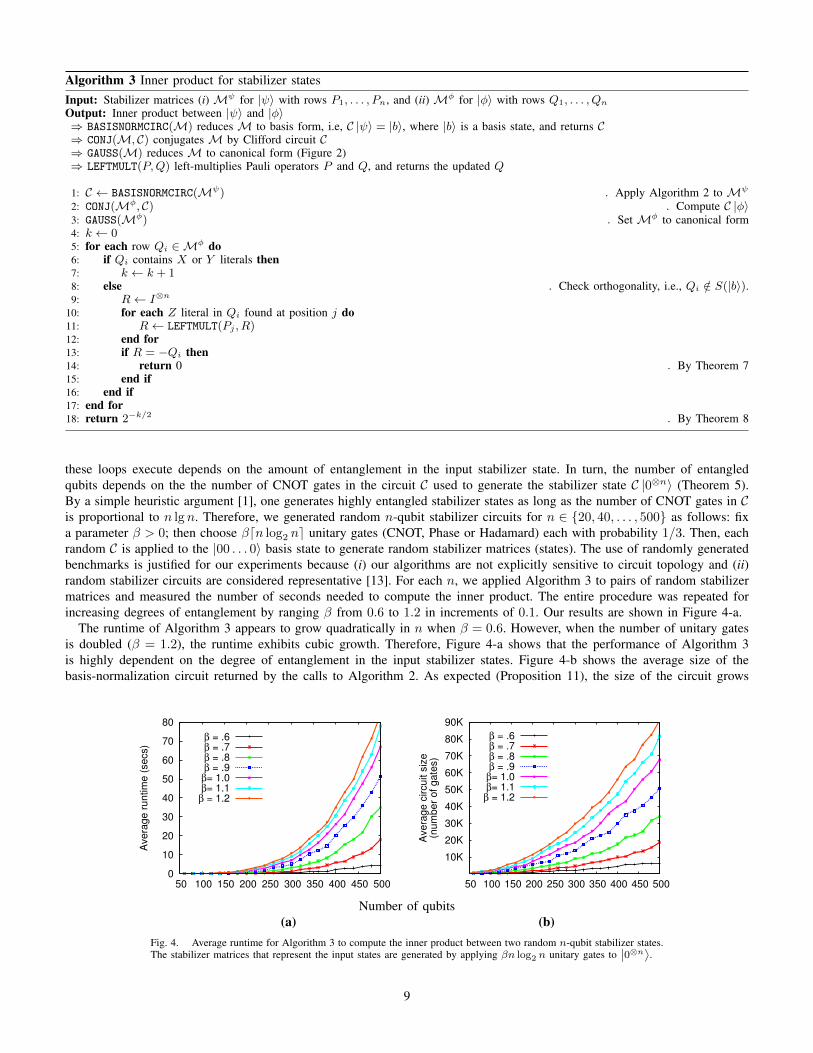
these loops execute depends on the amount of entanglement in the input stabilizer state. In turn, the number of entangledqubits depends on the the number of CNOT gates in the circuit C used to generate the stabilizer state C |0⊗n〉 (Theorem 5).By a simple heuristic argument [1], one generates highly entangled stabilizer states as long as the number of CNOT gates in Cis proportional to n lg n. Therefore, we generated random n-qubit stabilizer circuits for n ∈ 20, 40, . . . , 500 as follows: fixa parameter β > 0; then choose βdn log2 ne unitary gates (CNOT, Phase or Hadamard) each with probability 1/3. Then, eachrandom C is applied to the |00 . . . 0〉 basis state to generate random stabilizer matrices (states). The use of randomly generatedbenchmarks is justified for our experiments because (i) our algorithms are not explicitly sensitive to circuit topology and (ii)random stabilizer circuits are considered representative [13]. For each n, we applied Algorithm 3 to pairs of random stabilizermatrices and measured the number of seconds needed to compute the inner product. The entire procedure was repeated forincreasing degrees of entanglement by ranging β from 0.6 to 1.2 in increments of 0.1. Our results are shown in Figure 4-a.
The runtime of Algorithm 3 appears to grow quadratically in n when β = 0.6. However, when the number of unitary gatesis doubled (β = 1.2), the runtime exhibits cubic growth. Therefore, Figure 4-a shows that the performance of Algorithm 3is highly dependent on the degree of entanglement in the input stabilizer states. Figure 4-b shows the average size of thebasis-normalization circuit returned by the calls to Algorithm 2. As expected (Proposition 11), the size of the circuit grows
0
10
20
30
40
50
60
70
80
50 100 150 200 250 300 350 400 450 500
Ave
rag
e r
un
tim
e (
se
cs)
β = .6β = .7β = .8β = .9
β= 1.0β= 1.1
β = 1.2
10K
20K
30K
40K
50K
60K
70K
80K
90K
50 100 150 200 250 300 350 400 450 500
Ave
rag
e c
ircu
it s
ize
(nu
mb
er
of
ga
tes)
β = .6β = .7β = .8β = .9
β= 1.0β= 1.1
β = 1.2
Number of qubits(a) (b)
Fig. 4. Average runtime for Algorithm 3 to compute the inner product between two random n-qubit stabilizer states.The stabilizer matrices that represent the input states are generated by applying βn log2 n unitary gates to
∣∣0⊗n⟩.9

0
50
100
150
200
50 100 150 200 250 300 350 400 450 500
Ave
rag
e r
un
tim
e (
mill
ise
cs) ⟨00...0|φ⟩β = .6
β = .7β = .8β = .9
β= 1.0β= 1.1
β = 1.2
0
0.5
1.0
1.5
2.0
50 100 150 200 250 300 350 400 450 500
Ave
rag
e r
un
tim
e (
se
cs) ⟨GHZ|φ⟩β = .6
β = .7β = .8β = .9
β= 1.0β= 1.1
β = 1.2|φ=0...0⟩
Number of qubits(a) (b)
Fig. 5. Average runtime for Algorithm 3 to compute the inner product between (a)∣∣0⊗n⟩ and random stabilizer
state |φ〉 and (b) the n-qubit GHZ state and random stabilizer state |φ〉.
quadratically in n. Figure 5 shows the average runtime for Algorithm 3 to compute the inner product between: (i) the all-zeros basis state and random n-qubit stabilizer states, and (ii) the n-qubit GHZ state8 and random stabilizer states. GHZstates are maximally entangled states that have been realized experimentally using several quantum technologies and are oftenencountered in practical applications such as error-correcting codes and fault-tolerant architectures. Figure 5 shows that, forsuch practical instances, Algorithm 3 can compute the inner product in roughly O(n2) time (e.g. 〈GHZ|0〉). However, withoutapriori information about the input stabilizer matrices, one can only say that the performance of Algorithm 3 will be somewherebetween quadratic and cubic in n.
V. NEAREST-NEIGHBOR STABILIZER STATES
We used Algorithm 3 to compute the inner product between |00〉 and all two-qubit stabilizer states. Our results are shownin Table II. We leveraged these results to formulate the following properties related to the geometry of stabilizer states.
Definition 12. Given an arbitrary state |ψ〉 with ||ψ|| = 1, a stabilizer state |ϕ〉 is a nearest stabilizer state to |ψ〉 if |〈ψ|ϕ〉|attains the largest possible value 6= 1.
Proposition 13. Consider two orthogonal stabilizer states |α〉 and |β〉 whose unbiased superposition |ψ〉 is also a stabilizerstate. Then |ψ〉 is a nearest stabilizer state to |α〉 and |β〉.
Proof: Since stabilizer states are unbiased, |〈ψ|α〉| = |〈ψ|β〉| = 1√2
. By Theorem 8, this is the largest possible value 6= 1.Thus, |ψ〉 is a nearest stabilizer state to |α〉 and |β〉.
Lemma 14. For any two stabilizer states, the numbers of nearest-neighbor stabilizer states are equal.
Proof: By Corollary 6, any stabilizer state can be mapped to another stabilizer state by a stabilizer circuit. Since theoperators effected by these circuits are unitary, inner products are preserved.
Lemma 15. Let |ψ〉 and |ϕ〉 be orthogonal stabilizer states such that |ϕ〉 = P |ψ〉 where P is an element of the Pauli group.Then |ψ〉+|ϕ〉√
2is a stabilizer state.
Proof: Suppose |ψ〉 = 〈gk〉k=1,2,...,n is generated by elements gk of the n-qubit Pauli group. Let
f(k) =
0 if [P, gk] = 01 otherwise
and write |ϕ〉 = 〈(−1)f(k)gk〉. Conjugating each generator gk by P we see that |ϕ〉 is stabilized by 〈(−1)f(k)gk〉. Let Zk(respectively Xk) denote the Pauli operator Z (X) acting on the kth qubit. By Corollary 6, there exists an element L of then-qubit Clifford group such that L|ψ〉 = |0〉⊗n and L|ϕ〉 = (LPL†)L|ψ〉 = it|f(1)f(2) . . . f(n)〉. The second equality followsfrom the fact that LPL† is an element of the Pauli group and can therefore be written as itX(v)Z(u) for some t ∈ 0, 1, 2, 3and u, v ∈ Zk2 . Therefore, |ψ〉+ |ϕ〉√
2=L†(|0〉⊗n + it |f(1)f(2) . . . f(n)〉)√
2
8An n-qubit GHZ state is an equal superposition of the all-zeros and all-ones states, i.e., |0⊗n〉+|1⊗n〉√
2.
10

The state in parenthesis on the right-hand side is the product of an all-zeros state and a GHZ state. Therefore, the sum isstabilized by S′ = L†〈Szero, Sghz〉L where Szero = 〈Zi, i ∈ k|f(k) = 0〉 and Sghz is supported on k|f(k) = 1 andequals 〈(−1)t/2XX . . .X, ∀i ZiZi+1〉 if t = 0 mod 2 or 〈(−1)(t−1)/2Y Y . . . Y,∀i ZiZi+1〉 if t = 1 mod 2.
Theorem 16. For any n-qubit stabilizer state |ψ〉, there are 4(2n − 1) nearest-neighbor stabilizer states, and these states canbe produced as described in Lemma 15.
Proof: The all-zeros basis amplitude of any stabilizer state |ψ〉 that is a nearest neighbor to |0〉⊗n must be ∝ 1/√
2.Therefore, |ψ〉 is an unbiased superposition of |0〉⊗n and one of the other 2n− 1 basis states, i.e., |ψ〉 = |0〉⊗n+P |0〉⊗n
√2
, where
P ∈ Gn such that P |0〉⊗n 6= α |0〉⊗n. As in the proof of Lemma 15, we have |ψ〉 = |0〉⊗n+it|ϕ〉√2
, where |ϕ〉 is a basis stateand t ∈ 0, 1, 2, 3. Thus, there are 4 possible unbiased superpositions, and a total of 4(2n− 1) nearest stabilizer states. Since|0〉⊗n is a stabilizer state, all stabilizer states have the same number of nearest stabilizer states by Lemma 14.
Table II shows that |00〉 has 12 nearest-neighbor states. We computed inner products between all-pairs of 2-qubit stabilizerstates and confirmed that each had exactly 12 nearest neighbors. We used the same procedure to verify that all 3-qubit stabilizerstates have 28 nearest neighbors. We verified the correctness of our algorithm by comparing against inner product computationsbased on explicit basis amplitudes.
VI. STABILIZER FRAMES
Given an n-qubit stabilizer state |ψ〉, there exists an orthonormal basis including |ψ〉 and consisting entirely of stabilizerstates. Using Theorem 7, one can generate such a basis from the stabilizer representation of |ψ〉. Observe that, one can createa state |ϕ〉 that is orthogonal to |ψ〉 by changing the signs of an arbitrary non-empty subset of generators of S(|ψ〉), i.e., bypermuting the phase vector of the stabilizer matrix for |ψ〉. Moreover, selecting two different subsets will produce two mutuallyorthogonal states. Thus, one can produce 2n − 1 additional orthogonal stabilizer states. Such states, together with |ψ〉, forman orthonormal basis. This is illustrated by Table II were each row constitutes an orthonormal basis.
Definition 17. A stabilizer frame F is a set of k ≤ 2n stabilizer states that forms an orthonormal basis |ψ1〉 , . . . , |ψk〉 andspans a subspace of the n-qubit Hilbert space. F is represented by a pair consisting of (i) a stabilizer matrix M and (ii) a setof k distinct phase vectors σj(M), j ∈ 1, . . . , k. The size of the frame, which we denote by |F|, is equal to k.
Stabilizer frames are useful for representing arbitrary quantum states and for simulating the action of stabilizer circuits onsuch states. Let α = (α1, . . . , αk) ∈ Ck be the decomposition of the arbitrary n-qubit state |φ〉 onto the basis |ψ1〉 , . . . , |ψk〉defined by F , i.e., |φ〉 =
∑ki=1 αk |ψi〉. Furthermore, let U be a stabilizer gate. To simulate U |φ〉, one simply rotates the
basis defined by F to get the new basis U |ψ1〉 , . . . , U |ψk〉. This is accomplished with the following two-step process: (i)update the stabilizer matrix M associated with F as per Section II-A; (ii) iterate over the phase vectors in F and update eachaccordingly (Table III). The second step is linear in the number of phase vectors as only a constant number of elements ineach vector needs to be updated. Also, α may need to be updated, which requires the computation of the global phase of eachU |ψi〉. Since the stabilizer does not maintain global phases directly, each αi is updated as follows:
1. Use Gaussian elimination to obtain a basis state |b〉 from M (Observation 3) and store its non-zero amplitude β. If U isthe Hadamard gate, it may be necessary to sample a sum of two non-zero (one real, one imaginary) basis amplitudes.
2. Compute Uβ |b〉 = β′ |b′〉 directly using the state-vector representation.3. Obtain |b′〉 from UMU† and store its non-zero amplitude γ.4. Compute the global-phase factor generated as αi = (αi · β′)/γ.Observe that, all the above processes take time polynomial in k, therefore, if k = poly(n), U |φ〉 can be simulated efficiently
on a classical computer via frame-based simulation.
Inner product between frames. We now discuss how to use our algorithms to compute the inner product between arbitraryquantum states. Let |φ〉 and |ϕ〉 be quantum states represented by the pairs < Fφ, α = (α1, . . . , αk) > and < Fϕ, β =(β1, . . . , βl) >, respectively. The following steps compute |〈φ|ϕ〉|.
1. Apply Algorithm 2 to Mφ (the stabilizer matrix associated with Fφ) to obtain basis-normalization circuit C.2. Rotate frames Fφ and Fϕ by C as outlined in our previous discussion.3. Reduce Mφ to canonical form (Algorithm 1) and record the row operations applied. Apply the same row operations to
each phase vector σφi , i ∈ 1, . . . , k in Fφ. Repeat this step for Mϕ and the phase vectors in Fϕ.4. Let Mφ
i denote that the leading-phases of the rows in Mφ are set equal to σφi . Similarly, Mϕj denotes that the phases
of Mϕ are equal to σϕj . Furthermore, let δ(Mφi ,M
ϕj ) be the function that returns 0 if the orthogonality check from
Algorithm 3 (lines 9–15) returns 0, and 1 otherwise. The inner product is computed as,
|〈φ|ϕ〉| = 1
2s/2
k∑i=1
l∑j=1
|α∗i βj | · δ(Miφ,Mj
ϕ)
11

where s is the number of rows in Mϕ that contain X or Y literals.Prior work on representation of arbitrary states using the stabilizer formalism can be found in [1]. The authors propose an
approach that represents a quantum state as a sum of density-matrix terms. Our frame-based technique offers more compactstorage (|F| ≤ 2n whereas a density matrix may have 4n non-zero entries) but requires more sophisticated book-keeping.
VII. CONCLUSION
The stabilizer formalism facilitates compact representation of stabilizer states and efficient simulation of stabilizer circuits.Stabilizer states appear in many different quantum-information applications, and their efficient manipulation via geometric andlinear-algebraic operations may lead to additional insights. To this end, we study algorithms to efficiently compute the innerproduct between stabilizer states. A crucial step of this computation is the synthesis of a canonical circuit that transforms astabilizer state into a computational basis state. We designed an algorithm to synthesize such circuits using a 5-block templatestructure and showed that these circuits contain O(n2) stabilizer gates. We analysed the performance of our inner-productalgorithm and showed that, although its runtime is O(n3), there are practical instances in which it runs in linear or quadratictime. Furthermore, we proved that an n-qubit stabilizer state has exactly 4(2n − 1) nearest-neighbor states and verified thisresult experimentally. Finally, we designed techniques for representing arbitrary quantum states using stabilizer frames andgeneralize our algorithms to compute the inner product between two such frames.
REFERENCES
[1] S. Aaronson and D. Gottesman, “Improved simulation of stabilizer circuits,” Phys. Rev. A, vol. 70, no. 052328 (2004).[2] K. M. R. Audenaert and M. B. Plenio, “Entanglement on mixed stabiliser states: normal norms and reduction procedures,” New J. Phys.,
vol. 7, no. 170 (2005).[3] A. Calderbank, E. Rains, P. Shor, and N. Sloane, “Quantum error correction via codes over GF(4),” IEEE Trans. Inf. Theory, vol. 44,
pp. 1369–1387 (1998).[4] R. Cleve and D. Gottesman, “Efficient computations of encodings for quantum error correction,” Phys. Rev. A, vol. 56, no. 1 (1997).[5] J. Dehaene and B. De Moor, “Clifford group, stabilizer states, and linear and quadratic operations over GF(2),” Phys. Rev. A, vol. 68,
no. 042318 (2003).[6] I. Djordjevic, “Quantum information processing and quantum error correction: an engineering approach, ” Academic press (2012).[7] W. Dur, H. Aschauer and H.J. Briegel, “Multiparticle entanglement purification for graph states,” Phys. Rev. Lett., vol. 91, no. 10 (2003).[8] D. Fattal, T. S. Cubitto, Y. Yamamoto, S. Bravyi and I. L. Chuang, “Entanglement in the stabilizer formalism,” arXiv:0406168 (2004).[9] D. Gottesman, “Stabilizer codes and quantum error correction,” Caltech Ph.D. thesis (1997).[10] D. Gottesman, “The Heisenberg representation of quantum computers,” arXiv:9807006v1 (1998).[11] O. Guehne, G. Toth, P. Hyllus and H.J. Briegel,“Bell inequalities for graph states,” Phys. Rev. Lett., vol. 95, no. 120405 (2005).[12] M. Hein, J. Eisert, and H.J. Briegel,“Multi-party entanglement in graph states,” Phys. Rev. A, vol. 69, no. 6 (2004).[13] E. Knill, et. al., “Randomized benchmarking of quantum gates,” Phys. Rev. A, vol. 77, no. 1 (2007).[14] M. A. Nielsen and I. L. Chuang, “Quantum Computation and Quantum Information,” Cambridge University Press (2000).[15] K. N. Patel, I. L. Markov and J. P. Hayes, “Optimal synthesis of linear reversible circuits,” Quant. Inf. Comp., vol. 8, no. 3 (2008).[16] M. Van den Nest, “Classical simulation of quantum computation, the Gottesman-Knill theorem, and slightly beyond,” Quant. Inf. Comp.,
vol. 10, pp. 0258–0271 (2010).[17] M. Van den Nest, J. Dehaene and B. De Moor, “On local unitary versus local Clifford equivalence of stabilizer states,” Phys. Rev. A,
vol. 71, no. 062323 (2005).[18] H. Wunderlich and M. B. Plenio, “Quantitative verification of fidelities and entanglement from incomplete measurement data”, J. Mod.
Opt., vol. 56, pp. 2100–2105 (2009).
12

APPENDIX ATHE 1080 THREE-QUBIT STABILIZER STATES
Shorthand notation represents a stabilizer state as α0, α1, α2, α3 where αi are the normalized amplitudes of the basis states.Basis states are emphasized in bold. The ∠ column indicates the angle between that state and |000〉, which has 28 nearest-neighbor states and 315 orthogonal states (⊥).
STATE GEN’TORS STATE GEN’TORS STATE GEN’TORS STATE GEN’TORS STATE GEN’TORS STATE GEN’TORS STATE GEN’TORS STATE GEN’TORS
11111111 IIX IXI XII 1111---- IIX IXI -XII 100i-00i IXY IYX -XII 0i001000 IZI YIX -XIY 11----11 IIX -IXI -XII 1ii--ii1 IYZ -IXX -XII 10-00i0i XYX -IXZ -YYY 1--1-11- -IIX -IXI -XII1111iiii IIX IXI YII 1111iiii IIX IXI -YII 100ii001 IXY IYX -YII 1i00-i00 IZI YIX -XIZ 11--iiii IIX -IXI -YII 1ii-i-1i IYZ -IXX -YII 1ii-1ii- XYY -IXX -YIX 1--1iiii -IIX -IXI -YII
11110000 IIX IXI ZII 00001111 IIX IXI -ZII 0000100i IXY IYX -ZII 10000-00 IZI YIY -XIX 000011-- IIX -IXI -ZII 00001ii- IYZ -IXX -ZII 11--1-1- XYY -IXX -YYZ 00001--1 -IIX -IXI -ZII11ii11ii IIX IYI XII 11ii--ii IIX IYI -XII 1-ii-1ii IXY IYZ -XII 1-00--00 IZI YIY -XIZ 11ii--ii IIX -IYI -XII 11ii--ii IYZ -IXY -XII 1i-ii-i- XYY -IXZ -YIZ 1-ii-1ii -IIX -IYI -XII11iiii-- IIX IYI YII 11iiii11 IIX IYI -YII 1-iiii11 IXY IYZ -YII 1i00i-00 IZI YIZ -XIX 11iiii-- IIX -IYI -YII 11iiii1- IYZ -IXY -YII 0-0-10-0 XYY -IXZ -YYX 1-iiii-1 -IIX -IYI -YII
11ii0000 IIX IYI ZII 000011ii IIX IYI -ZII 00001-ii IXY IYZ -ZII 1100ii00 IZI YIZ -XIY 000011ii IIX -IYI -ZII 000011ii IYZ -IXY -ZII 100-0ii0 XYZ -IXX -YIX 00001-ii -IIX -IYI -ZII11001100 IIX IZI XII 1100--00 IIX IZI -XII 0i100i10 IXY XII -IYX 1-000000 IZI ZII -IIX 001100-- IIX -IZI -XII 11ii-1ii IYZ -XIZ -YXX 1-1-iiii XYZ -IXX -YYY 001-00-1 -IIX -IZI -XII1100ii00 IIX IZI YII 1100ii00 IIX IZI -YII 11ii11ii IXY XII -IYZ 1i000000 IZI ZII -IIY 001100ii IIX -IZI -YII 1ii1-ii1 IYZ -XIZ -YXY 100i01i0 XYZ -IXY -YIY 001-00ii -IIX -IZI -YII11000000 IIX IZI ZII 00001100 IIX IZI -ZII 11iiii11 IXY XIY -YYX 01000000 IZI ZII -IIZ 00000011 IIX -IZI -ZII 1-iiii1- IYZ -XXX -YIZ 1i-ii1i1 XYZ -IXY -YYX 0000001- -IIX -IZI -ZII00111100 IIX XXI YYI 11--11-- IIX XII -IXI 100i0i10 IXY XIY -YYZ 111-11-1 IZX XIX -YXY 00--1100 IIX -XXI -YYI 0i0-10i0 IYZ -XXX -YXY 1-ii1-ii XZI -IIX -YXI 00-11-00 -IIX -XXI -YYI11iiii11 IIX XXI YZI 11ii11ii IIX XII -IYI 1-ii11ii IXY XYX -YIY 11ii11ii IZX XIX -YXZ 11iiii-- IIX -XXI -YZI 1ii-i11i IYZ -XXY -YIZ 1--11-1- XZI -IIX -YYI 1-iiii-1 -IIX -XXI -YZI110000ii IIX XYI YXI 00110011 IIX XII -IZI 1i-i1i1i IXY XYX -YYZ 11-1iiii IZX XXY -YIX 110000ii IIX -XYI -YXI 10i0010i IYZ -XXY -YXX 1ii11ii- XZI -IIY -YXI 1-0000ii -IIX -XYI -YXI11--iiii IIX XYI YZI 11000011 IIX XXI -YYI 0-i0100i IXY XYZ -YIY 110000ii IZX XXY -YXZ 11--iiii IIX -XYI -YZI 1-00-100 IZI -IIX -XII 1i-i1i1i XZI -IIY -YYI 1--1iiii -IIX -XYI -YZI11ii11ii IIX XZI YXI 11iiii11 IIX XXI -YZI 1i1ii-i1 IXY XYZ -YYX 11iiii1- IZX XXZ -YIX 11ii--ii IIX -XZI -YXI 1-00ii00 IZI -IIX -YII 010i010i XZI -IIZ -YXI 1-ii-1ii -IIX -XZI -YXI111111-- IIX XZI YYI 00ii1100 IIX XYI -YXI 0i100-i0 IXY YII -IYX 001-1100 IZX XXZ -YXY 1111--11 IIX -XZI -YYI 00001-00 IZI -IIX -ZII 010-0101 XZI -IIZ -YYI 1-1--11- -IIX -XZI -YYI1i1i1i1i IIY IXI XII 1111iiii IIX XYI -YZI 11iiii1- IXY YII -IYZ 11-1iiii IZX YIX -XXY 1i-i-i1i IIY -IXI -XII 1i00-i00 IZI -IIY -XII 1--1iiii YII -IIX -IXI 1i-i-i1i -IIY -IXI -XII1i1ii-i- IIY IXI YII 11ii11ii IIX XZI -YXI 1-ii--ii IXY YIY -XYX 11iiii-1 IZX YIX -XXZ 1i-ii1i- IIY -IXI -YII 1i00i-00 IZI -IIY -YII 1-iiii1- YII -IIX -IYI 1i-ii-i1 -IIY -IXI -YII
1i1i0000 IIY IXI ZII 11--1111 IIX XZI -YYI 01i0100i IXY YIY -XYZ 111---1- IZX YXY -XIX 00001i-i IIY -IXI -ZII 00001i00 IZI -IIY -ZII 001-00ii YII -IIX -IZI 00001i-i -IIY -IXI -ZII1ii-1ii- IIY IYI XII 11--iiii IIX YII -IXI 11iiii-- IXY YYX -XIY 00-11100 IZX YXY -XXZ 1ii1-ii- IIY -IYI -XII 01000-00 IZI -IIZ -XII 1i-ii1i- YII -IIY -IXI 1ii--ii1 -IIY -IYI -XII1ii-i--i IIY IYI YII 11iiii11 IIX YII -IYI 1i1ii1i- IXY YYX -XYZ 11ii--ii IZX YXZ -XIX 1ii1i1-i IIY -IYI -YII 01000i00 IZI -IIZ -YII 1ii-i11i YII -IIY -IYI 1ii-i--i -IIY -IYI -YII
1ii-0000 IIY IYI ZII 001100ii IIX YII -IZI 100i0i-0 IXY YYZ -XIY 110000ii IZX YXZ -XXY 00001ii1 IIY -IYI -ZII 00000100 IZI -IIZ -ZII 001i00i1 YII -IIY -IZI 00001ii- -IIY -IYI -ZII1i001i00 IIY IZI XII 00ii1100 IIX YXI -XYI 1i-i-i-i IXY YYZ -XYX 1i-i1i1i IZY XIY -YXX 001i00-i IIY -IZI -XII 0-001000 IZI -XIX -YIY 010-0i0i YII -IIZ -IXI 001i00-i -IIY -IZI -XII1i00i-00 IIY IZI YII 11ii--ii IIX YXI -XZI 0i100000 IXY ZII -IYX 1ii11ii- IZY XIY -YXZ 001i00i1 IIY -IZI -YII 1i00i-00 IZI -XIX -YIZ 010i0i01 YII -IIZ -IYI 001i00i- -IIY -IZI -YII1i000000 IIY IZI ZII 110000-- IIX YYI -XXI 11ii0000 IXY ZII -IYZ 1i1ii1i1 IZY XXX -YIY 0000001i IIY -IZI -ZII 10000i00 IZI -XIY -YIX 0001000i YII -IIZ -IZI 0000001i -IIY -IZI -ZII001i1i00 IIY XXI YYI 11------ IIX YYI -XZI 1i1i-i-i IXZ IYX -XII 00i11i00 IZY XXX -YXZ 00-i1i00 IIY -XXI -YYI 1-00ii00 IZI -XIY -YIZ 0-100ii0 YII -IXX -IYY 00-i1i00 -IIY -XXI -YYI1ii-i-1i IIY XXI YZI 11iiii-- IIX YZI -XXI 1i1ii-i1 IXZ IYX -YII 1ii-i11i IZY XXZ -YIY 1ii-i1-i IIY -XXI -YZI 1i00-i00 IZI -XIZ -YIX 1ii-i-1i YII -IXX -IYZ 1ii1i--i -IIY -XXI -YZI1i0000i- IIY XYI YXI 1111iiii IIX YZI -XYI 00001i1i IXZ IYX -ZII 1i00001i IZY XXZ -YXX 1i0000i1 IIY -XYI -YXI 1100-100 IZI -XIZ -YIY 100ii001 YII -IXY -IYX 1i0000i- -IIY -XYI -YXI1i-ii-i- IIY XYI YZI 11--0000 IIX ZII -IXI 111----1 IXZ IYY -XII 1i1ii-i- IZY YIY -XXX 1i-ii1i1 IIY -XYI -YZI 11-1---1 IZX -XIX -YXY 1-iiii11 YII -IXY -IYZ 1i-ii-i- -IIY -XYI -YZI1ii11ii- IIY XZI YXI 11ii0000 IIX ZII -IYI 111-iiii IXZ IYY -YII 1ii-i--i IZY YIY -XXZ 1ii1-ii1 IIY -XZI -YXI 11ii--ii IZX -XIX -YXZ 1i-ii1i1 YII -IXZ -IYX 1ii--ii- -IIY -XZI -YXI1i1i1i-i IIY XZI YYI 00110000 IIX ZII -IZI 0000111- IXZ IYY -ZII 1i-i-i-i IZY YXX -XIY 1i1i-i1i IIY -XZI -YYI 111-iiii IZX -XXY -YIX 11-1iiii YII -IXZ -IYY 1i1i-i1i -IIY -XZI -YYI
10101010 IIZ IXI XII 1i1i-i-i IIY IXI -XII 1i1i1i1i IXZ XII -IYX 1i0000-i IZY YXX -XXZ 10-0-010 IIZ -IXI -XII 00ii1100 IZX -XXY -YXZ 0i0i10-0 YIX -IXI -XIY 010-0-01 -IIZ -IXI -XII1010i0i0 IIZ IXI YII 1i1ii1i1 IIY IXI -YII 1-111-11 IXZ XII -IYY 1ii1-ii1 IZY YXZ -XIY 10-0i0i0 IIZ -IXI -YII 11iiii-1 IZX -XXZ -YIX 1i-i-i1i YIX -IXI -XIZ 010-0i0i -IIZ -IXI -YII10100000 IIZ IXI ZII 00001i1i IIY IXI -ZII 111-1-11 IXZ XIZ -YYX 00i-1i00 IZY YXZ -XXX 000010-0 IIZ -IXI -ZII 110000-1 IZX -XXZ -YXY 1ii--ii1 YIX -IXX -XYY 0000010- -IIZ -IXI -ZII10i010i0 IIZ IYI XII 1ii--ii1 IIY IYI -XII 1i1i1i1i IXZ XIZ -YYY 100i100i IZZ XIZ -YXX 10i0-0i0 IIZ -IYI -XII 1i1i-i1i IZY -XIY -YXX 100-0ii0 YIX -IXX -XYZ 010i0-0i -IIZ -IYI -XII10i0i0-0 IIZ IYI YII 1ii-i11i IIY IYI -YII 1-11iiii IXZ XYX -YIZ 100-1001 IZZ XIZ -YXY 10i0i0-0 IIZ -IYI -YII 1ii--ii- IZY -XIY -YXZ 0i0-10i0 YIX -IYI -XIY 010i0i0- -IIZ -IYI -YII10i00000 IIZ IYI ZII 00001ii- IIY IYI -ZII 10100i0i IXZ XYX -YYY 100ii001 IZZ XXX -YIZ 000010i0 IIZ -IYI -ZII 1i-ii1i- IZY -XXX -YIY 1ii1-ii1 YIX -IYI -XIZ 0000010i -IIZ -IYI -ZII10001000 IIZ IZI XII 1i00-i00 IIY IZI -XII 1i1ii1i- IXZ XYY -YIZ 10000001 IZZ XXX -YXY 001000-0 IIZ -IZI -XII 1i0000i- IZY -XXX -YXZ 1i-i1i1i YIX -IYX -XXY 0001000- -IIZ -IZI -XII1000i000 IIZ IZI YII 1i00i100 IIY IZI -YII 010-1010 IXZ XYY -YYX 1001i00i IZZ XXY -YIZ 001000i0 IIZ -IZI -YII 1ii1i1-i IZY -XXZ -YIY 0i-0100i YIX -IYX -XXZ 0001000i -IIZ -IZI -YII10000000 IIZ IZI ZII 00001i00 IIY IZI -ZII 1i1ii-i1 IXZ YII -IYX 000i1000 IZZ XXY -YXX 00000010 IIZ -IZI -ZII 00-i1i00 IZY -XXZ -YXX 000i0010 YIX -IZI -XIY 00000001 -IIZ -IZI -ZII00101000 IIZ XXI YYI 1i-i1i-i IIY XII -IXI 1-11iiii IXZ YII -IYY 100ii00- IZZ YIZ -XXX 00-01000 IIZ -XXI -YYI 100i-00i IZZ -XIZ -YXX 001i00-i YIX -IZI -XIZ 000-0100 -IIZ -XXI -YYI10i0i010 IIZ XXI YZI 1ii11ii1 IIY XII -IYI 1-11iiii IXZ YIZ -XYX 1001i00i IZZ YIZ -XXY 10i0i0-0 IIZ -XXI -YZI 1001-001 IZZ -XIZ -YXY 1---iiii YIX -IZX -XXY 010i0i0- -IIZ -XXI -YZI100000i0 IIZ XYI YXI 001i001i IIY XII -IZI 1i1ii-i1 IXZ YIZ -XYY 100i-00i IZZ YXX -XIZ 100000i0 IIZ -XYI -YXI 100ii00- IZZ -XXX -YIZ 1-iiii-- YIX -IZX -XXZ 0100000i -IIZ -XYI -YXI10-0i0i0 IIZ XYI YZI 1i00001i IIY XXI -YYI 111--1-- IXZ YYX -XIZ 000i1000 IZZ YXX -XXY 10-0i0i0 IIZ -XYI -YZI 000-1000 IZZ -XXX -YXY 10-00-01 YIY -IXI -XIX 010-0i0i -IIZ -XYI -YZI10i010i0 IIZ XZI YXI 1ii1i11i IIY XXI -YZI 0-011010 IXZ YYX -XYY 100--00- IZZ YXY -XIZ 10i0-0i0 IIZ -XZI -YXI 100-i00i IZZ -XXY -YIZ 1--1--11 YIY -IXI -XIZ 010i0-0i -IIZ -XZI -YXI101010-0 IIZ XZI YYI 00i-1i00 IIY XYI -YXI 1i1i-i-i IXZ YYY -XIZ 1000000- IZZ YXY -XXX 1010-010 IIZ -XZI -YYI 1000000i IZZ -XXY -YXX 11ii1-ii YIY -IXY -XYX 01010-01 -IIZ -XZI -YYI01011010 IXI XIX YIY 1i1ii1i- IIY XYI -YZI 10100i0i IXZ YYY -XYX 010-10-0 XIX YIY -IXI 1-1--1-1 IXI -IIX -XII 1--11--1 XII -IIX -IXI 100i0-i0 YIY -IXY -XYZ 0-0110-0 -IXI -XIX -YIY1i1ii1i1 IXI XIX YIZ 1ii-1ii1 IIY XZI -YXI 1i1i0000 IXZ ZII -IYX 010i10i0 XIX YIY -IYI 1-1-iiii IXI -IIX -YII 1-ii1-ii XII -IIX -IYI 10i00-0i YIY -IYI -XIX 1i-ii-i1 -IXI -XIX -YIZ10100i0i IXI XIY YIX 1i-i1i1i IIY XZI -YYI 1-110000 IXZ ZII -IYY 00010010 XIX YIY -IZI 00001-1- IXI -IIX -ZII 001-001- XII -IIX -IZI 1-ii--ii YIY -IYI -XIZ 10-00i0i -IXI -XIY -YIX1-1-iiii IXI XIY YIZ 1i-ii-i1 IIY YII -IXI 1-ii1-ii IYI XII -IIX 1i-ii1i- XIX YIZ -IXI 1i1i-i-i IXI -IIY -XII 1i-i1i-i XII -IIY -IXI 1-11--1- YIY -IYY -XXX 1--1iiii -IXI -XIY -YIZ1i1i1i1i IXI XIZ YIX 1ii1i-1i IIY YII -IYI 1ii11ii1 IYI XII -IIY 1ii1i11i XIX YIZ -IYI 1i1ii-i- IXI -IIY -YII 1ii-1ii- XII -IIY -IYI 01-01001 YIY -IYY -XXZ 1i-i-i1i -IXI -XIZ -YIX11111-1- IXI XIZ YIY 001i00i- IIY YII -IZI 010i010i IYI XII -IIZ 001i00i1 XIX YIZ -IZI 00001i1i IXI -IIY -ZII 001i001i XII -IIY -IZI 0010000- YIY -IZI -XIX 11---11- -IXI -XIZ -YIY01100110 IXX IYY XII 00i11i00 IIY YXI -XYI 10i0010i IYI XIX -YIY 1i-ii1i- XIX YXY -IYX 01010-0- IXI -IIZ -XII 010-010- XII -IIZ -IXI 001-00-- YIY -IZI -XIZ 0-1001-0 -IXX -IYY -XII01100ii0 IXX IYY YII 1ii--ii- IIY YXI -XZI 1ii1i11i IYI XIX -YIZ 1----1-- XIX YXY -IZX 01010i0i IXI -IIZ -YII 010i010i XII -IIZ -IYI 1i1ii-i- YIY -IZY -XXX 0-100ii0 -IXX -IYY -YII01100000 IXX IYY ZII 1i0000-i IIY YYI -XXI 0i0-10i0 IYI XIY -YIX 01i0100i XIX YXZ -IYX 00000101 IXI -IIZ -ZII 00010001 XII -IIZ -IZI 1ii-i--i YIY -IZY -XXZ 00000-10 -IXX -IYY -ZII1ii11ii1 IXX IYZ XII 1i-i-i-i IIY YYI -XZI 11iiii1- IYI XIY -YIZ 1-ii-1ii XIX YXZ -IZX 0-0-1010 IXI -XIX -YIY 0-100-10 XII -IXX -IYY 1i-ii-i1 YIZ -IXI -XIX 1ii--ii1 -IXX -IYZ -XII1ii1i--i IXX IYZ YII 1ii1i--i IIY YZI -XXI 1ii-1ii1 IYI XIZ -YIX 1ii-i1-i XIX YYY -IXX 1i1ii-i- IXI -XIX -YIZ 1ii-1ii- XII -IXX -IYZ 11--iiii YIZ -IXI -XIY 1ii-i1-i -IXX -IYZ -YII
1ii10000 IXX IYZ ZII 1i1ii-i1 IIY YZI -XYI 1-ii11ii IYI XIZ -YIY 100-01-0 XIX YYZ -IXX 10100i0i IXI -XIY -YIX 100i100i XII -IXY -IYX 11-1iiii YIZ -IXZ -XYX 00001ii- -IXX -IYZ -ZII1ii1i11i IXX XIX YYY 1i-i0000 IIY ZII -IXI 1-iiii-1 IYI YII -IIX 10-00i0i XIY YIX -IXI 1-1-iiii IXI -XIY -YIZ 1-ii1-ii XII -IXY -IYZ 1i-ii1i1 YIZ -IXZ -XYY 1ii-i-1i -IXX -XIX -YYY
01101001 IXX XIX YYZ 1ii10000 IIY ZII -IYI 1ii1i1-i IYI YII -IIY 10i00i01 XIY YIX -IYI 1i1i-i-i IXI -XIZ -YIX 1i-i1i-i XII -IXZ -IYX 1ii-i-1i YIZ -IYI -XIX 100-0-10 -IXX -XIX -YYZ1ii1-ii- IXX XYY YIX 001i0000 IIY ZII -IZI 010i0i0- IYI YII -IIZ 0010000i XIY YIX -IZI 1111-1-1 IXI -XIZ -YIY 11-111-1 XII -IXZ -IYY 11iiii1- YIZ -IYI -XIY 1ii--ii1 -IXX -XYY -YIX1--1---- IXX XYY YYZ 1010-0-0 IIZ IXI -XII 0i0110i0 IYI YIX -XIY 1--1iiii XIY YIZ -IXI 1001-00- IXX -IYY -XII 10-0010- XIX -IXI -YIY 1-iiii1- YIZ -IYZ -XXX 1-1---11 -IXX -XYY -YYZ
10010ii0 IXX XYZ YIX 1010i0i0 IIZ IXI -YII 1ii--ii- IYI YIX -XIZ 1-iiii11 XIY YIZ -IYI 1001i00i IXX -IYY -YII 1i-ii1i- XIX -IXI -YIZ 1ii1i-1i YIZ -IYZ -XXY 0ii0100- -IXX -XYZ -YIX1111iiii IXX XYZ YYY 00001010 IIZ IXI -ZII 10i00-0i IYI YIY -XIX 001-00ii XIY YIZ -IZI 00001001 IXX -IYY -ZII 1ii-i1-i XIX -IXX -YYY 001i00i- YIZ -IZI -XIX 11--iiii -IXX -XYZ -YYY100i100i IXY IYX XII 10i0-0i0 IIZ IYI -XII 1-ii--ii IYI YIY -XIZ 1-11iiii XIY YXX -IYY 1ii1-ii- IXX -IYZ -XII 01-0100- XIX -IXX -YYZ 001100ii YIZ -IZI -XIY 100i-00i -IXY -IYX -XII100ii00- IXY IYX YII 10i0i010 IIZ IYI -YII 1ii1i--i IYI YIZ -XIX 1i1i-i1i XIY YXX -IZY 1ii1i--i IXX -IYZ -YII 10i0010i XIX -IYI -YIY 0i100-i0 YIZ -IZZ -XXX 100ii00- -IXY -IYX -YII100i0000 IXY IYX ZII 000010i0 IIZ IYI -ZII 11iiii-1 IYI YIZ -XIY 0ii01001 XIY YXZ -IYY 00001ii1 IXX -IYZ -ZII 1ii-i1-i XIX -IYI -YIZ 01100ii0 YIZ -IZZ -XXY 0000100i -IXY -IYX -ZII1-ii1-ii IXY IYZ XII 1000-000 IIZ IZI -XII 1-ii0000 IYI ZII -IIX 1ii--ii- XIY YXZ -IZY 1ii1i--i IXX -XIX -YYY 1i1ii1i1 XIX -IYX -YXY 00ii1-00 YXI -IIX -XYI 1-ii-1ii -IXY -IYZ -XII1-iiii-- IXY IYZ YII 1000i000 IIZ IZI -YII 1ii10000 IYI ZII -IIY 11iiii-- XIY YYX -IXY 0--01001 IXX -XIX -YYZ 100i01i0 XIX -IYX -YXZ 1-ii-1ii YXI -IIX -XZI 1-iiii-- -IXY -IYZ -YII
1-ii0000 IXY IYZ ZII 00001000 IIZ IZI -ZII 010i0000 IYI ZII -IIZ 100i0i-0 XIY YYZ -IXY 1ii11ii1 IXX -XYY -YIX 00100001 XIX -IZI -YIY 00i-1i00 YXI -IIY -XYI 00001-ii -IXY -IYZ -ZII1-iiii1- IXY XIY YYX 10-010-0 IIZ XII -IXI 0i100i10 IYX XII -IXY 1i-i1i-i XIZ YIX -IXI 1--11111 IXX -XYY -YYZ 001i00i1 XIX -IZI -YIZ 1ii1-ii1 YXI -IIY -XZI 11iiii11 -IXY -XIY -YYX
0i10100i IXY XIY YYZ 10i010i0 IIZ XII -IYI 1i-i1i-i IYX XII -IXZ 1ii-1ii1 XIZ YIX -IYI 10010ii0 IXX -XYZ -YIX 1-11-111 XIX -IZX -YXY 000i0100 YXI -IIZ -XYI 100i0i10 -IXY -XIY -YYZ11ii1-ii IXY XYX YIY 00100010 IIZ XII -IZI 1i1ii1i1 IYX XIX -YXY 001i001i XIZ YIX -IZI 1111iiii IXX -XYZ -YYY 1-ii-1ii XIX -IZX -YXZ 010i0-0i YXI -IIZ -XZI 1-ii11ii -IXY -XYX -YIY1i1i1i-i IXY XYX YYZ 10000010 IIZ XXI -YYI 01i0100i IYX XIX -YXZ 11--1--1 XIZ YIY -IXI 0i100i-0 IXY -IYX -XII 0i0i10-0 XIY -IXI -YIX 11-1iiii YXX -IYY -XIY 1i-i1i1i -IXY -XYX -YYZ100i0-i0 IXY XYZ YIY 10i0i010 IIZ XXI -YZI 1i-i1i1i IYX XXY -YIX 11ii1-ii XIZ YIY -IYI 0i1001i0 IXY -IYX -YII 11--iiii XIY -IXI -YIZ 1ii1i1-i YXX -IYY -XXZ 0-i0100i -IXY -XYZ -YIY1i-ii-i- IXY XYZ YYX 00i01000 IIZ XYI -YXI 11ii1-ii IYX XXY -YXZ 0011001- XIZ YIY -IZI 00000i10 IXY -IYX -ZII 1-iiii-1 XIY -IXY -YYX 11ii-1ii YXX -IYZ -XIZ 1i1ii-i1 -IXY -XYZ -YYX
1i1i1i1i IXZ IYX XII 1010i0i0 IIZ XYI -YZI 100i0i10 IYX XXZ -YIX 1-ii11ii XIZ YXX -IYZ 11ii--ii IXY -IYZ -XII 0i-0100i XIY -IXY -YYZ 0-0i10i0 YXX -IYZ -XXY 1i-i-i1i -IXZ -IYX -XII1i1ii1i- IXZ IYX YII 10i010i0 IIZ XZI -YXI 1-iiii11 IYX XXZ -YXY 0i100i10 XIZ YXX -IZZ 11iiii-1 IXY -IYZ -YII 0i0110i0 XIY -IYI -YIX 1i-i1i1i YXX -IZY -XIY 1i-ii-i- -IXZ -IYX -YII1i1i0000 IXZ IYX ZII 10-01010 IIZ XZI -YYI 0i1001i0 IYX YII -IXY 1ii11ii- XIZ YXY -IYZ 000011ii IXY -IYZ -ZII 11iiii-1 XIY -IYI -YIZ 00-i1i00 YXX -IZY -XXZ 00001i-i -IXZ -IYX -ZII111-111- IXZ IYY XII 10-0i0i0 IIZ YII -IXI 1i-ii-i- IYX YII -IXZ 01100-10 XIZ YXY -IZZ 1-iiii-1 IXY -XIY -YYX 11-1iiii XIY -IYY -YXX 0i100i-0 YXX -IZZ -XIZ 11-1--1- -IXZ -IYY -XII111-iiii IXZ IYY YII 10i0i010 IIZ YII -IYI 1i-i-i-i IYX YIX -XXY 11-11--- XIZ YYX -IXZ 0i-0100i IXY -XIY -YYZ 10010ii0 XIY -IYY -YXZ 0i000010 YXX -IZZ -XXY 11-1iiii -IXZ -IYY -YII
111-0000 IXZ IYY ZII 001000i0 IIZ YII -IZI 100i0i-0 IYX YIX -XXZ 1i-i1i-i XIZ YYY -IXZ 11ii-1ii IXY -XYX -YIY 000i0010 XIY -IZI -YIX 1i1ii-i- YXY -IYX -XIX 000011-1 -IXZ -IYY -ZII1-11111- IXZ XIZ YYX 00i01000 IIZ YXI -XYI 1i1ii-i- IYX YXY -XIX 001-1-00 XXI YYI -IIX 1i1i-i1i IXY -XYX -YYZ 001100ii XIY -IZI -YIZ 1-iiii-- YXY -IYX -XXZ 11-1-111 -IXZ -XIZ -YYX1i1i1i1i IXZ XIZ YYY 10i0-0i0 IIZ YXI -XZI 1-iiii-- IYX YXY -XXZ 001i1i00 XXI YYI -IIY 100i01i0 IXY -XYZ -YIY 1i-i-i-i XIY -IZY -YXX 1ii--ii- YXY -IYZ -XIZ 1i-i-i1i -IXZ -XIZ -YYY111-iiii IXZ XYX YIZ 100000-0 IIZ YYI -XXI 0-i0100i IYX YXZ -XIX 00010100 XXI YYI -IIZ 1i-ii1i1 IXY -XYZ -YYX 1ii1-ii1 XIY -IZY -YXZ 10i00i0- YXY -IYZ -XXX 1---iiii -IXZ -XYX -YIZ0i0i1010 IXZ XYX YYY 10-0-0-0 IIZ YYI -XZI 11ii-1ii IYX YXZ -XXY 1-iiii1- XXI YZI -IIX 1i1i-i-i IXZ -IYX -XII 1i-i1i-i XIZ -IXI -YIX 1-111--- YXY -IZX -XIX 0i0i10-0 -IXZ -XYX -YYY1i1ii1i- IXZ XYY YIZ 10i0i0-0 IIZ YZI -XXI 0i100000 IYX ZII -IXY 1ii1i11i XXI YZI -IIY 1i1ii1i- IXZ -IYX -YII 1--111-- XIZ -IXI -YIY 1-0000-- YXY -IZX -XXZ 1i-ii1i1 -IXZ -XYY -YIZ
1010010- IXZ XYY YYX 1010i0i0 IIZ YZI -XYI 1i-i0000 IYX ZII -IXZ 010i0i01 XXI YZI -IIZ 00001i1i IXZ -IYX -ZII 1---11-1 XIZ -IXZ -YYX 0-100--0 YXY -IZZ -XIZ 10-00101 -IXZ -XYY -YYX010i10i0 IYI XIX YIY 10-00000 IIZ ZII -IXI 100-100- IYY XII -IXX 11-11-11 XXX YIY -IYY 1-11-1-- IXZ -IYY -XII 1i-i1i-i XIZ -IXZ -YYY 00100-00 YXY -IZZ -XXX 0-0i10i0 -IYI -XIX -YIY1ii-i1-i IYI XIX YIZ 10i00000 IIZ ZII -IYI 1---1--- IYY XII -IXZ 1i-ii-i1 XXX YIY -IZY 1-11iiii IXZ -IYY -YII 1ii11ii- XIZ -IYI -YIX 100i0-i0 YXZ -IYX -XIX 1ii1i--i -IYI -XIX -YIZ10i00i0- IYI XIY YIX 00100000 IIZ ZII -IZI 1---iiii IYY XIY -YXX 11iiii11 XXX YIZ -IYZ 00001-11 IXZ -IYY -ZII 1-ii11ii XIZ -IYI -YIY 11ii1-ii YXZ -IYX -XXY 10i00i0- -IYI -XIY -YIX1-iiii-- IYI XIY YIZ 1-1-1-1- IXI XII -IIX 0ii0100- IYY XIY -YXZ 0i1001i0 XXX YIZ -IZZ 1-11---1 IXZ -XIZ -YYX 11ii1-ii XIZ -IYZ -YXX 10010ii0 YXZ -IYY -XIY 1-iiii-- -IYI -XIY -YIZ1ii11ii- IYI XIZ YIX 1i1i1i1i IXI XII -IIY 111--111 IYY XXX -YIY 0i0110i0 XXX YXY -IYZ 1i1i-i-i IXZ -XIZ -YYY 1ii-1ii1 XIZ -IYZ -YXY 1ii1-ii- YXZ -IYY -XXX 1ii--ii- -IYI -XIZ -YIX11ii1-ii IYI XIZ YIY 01010101 IXI XII -IIZ 1ii--ii1 IYY XXX -YXZ 01000010 XXX YXY -IZZ 111-iiii IXZ -XYX -YIZ 001i001i XIZ -IZI -YIX 1-ii1-ii YXZ -IZX -XIX 11ii-1ii -IYI -XIZ -YIY1i-ii1i- IYX XIX YXY 10100101 IXI XIX -YIY 100-0110 IYY XXZ -YIY 1ii11ii1 XXX YXZ -IYY 0i0i1010 IXZ -XYX -YYY 001-0011 XIZ -IZI -YIY 00ii1-00 YXZ -IZX -XXY 1i-ii-i1 -IYX -XIX -YXY
100i01i0 IYX XIX YXZ 1i1ii1i1 IXI XIX -YIZ 1ii-i11i IYY XXZ -YXX 00i11i00 XXX YXZ -IZY 1i1ii-i1 IXZ -XYY -YIZ 0i100i10 XIZ -IZZ -YXX 1ii11ii- YXZ -IZY -XIY 0-i0100i -IYX -XIX -YXZ1i1i1i-i IYX XXY YIX 0i0i1010 IXI XIY -YIX 100-i00i IYY YII -IXX 1i1i-i1i XXY YIX -IYX 10100-01 IXZ -XYY -YYX 0-100110 XIZ -IZZ -YXY 1i0000i- YXZ -IZY -XXX 1i1i1i-i -IYX -XXY -YIX1-ii11ii IYX XXY YXZ 1111iiii IXI XIY -YIZ 1---iiii IYY YII -IXZ 1-11iiii XXY YIX -IZX 1-ii-1ii IYI -IIX -XII 1-00001- XXI -IIX -YYI 1-0000-1 YYI -IIX -XXI 1-ii11ii -IYX -XXY -YXZ0i10100i IYX XXZ YIX 1i1i1i1i IXI XIZ -YIX 111-1--- IYY YIY -XXX 1ii-i11i XXY YIZ -IYZ 1-iiii1- IYI -IIX -YII 1-iiii1- XXI -IIX -YZI 1--1-1-1 YYI -IIX -XZI 100i0i-0 -IYX -XXZ -YIX11iiii1- IYX XXZ YXY 1-1-1111 IXI XIZ -YIY 100-0--0 IYY YIY -XXZ 0-100ii0 XXY YIZ -IZZ 00001-ii IYI -IIX -ZII 1i00001i XXI -IIY -YYI 1i0000-i YYI -IIY -XXI 11iiii-1 -IYX -XXZ -YXY111-iiii IYY XIY YXX 1-1-iiii IXI YII -IIX 1---iiii IYY YXX -XIY 10i0010i XXY YXX -IYZ 1ii1-ii- IYI -IIY -XII 1ii-i-1i XXI -IIY -YZI 1i-i-i-i YYI -IIY -XZI 1-11iiii -IYY -XIY -YXX100-0ii0 IYY XIY YXZ 1i1ii1i1 IXI YII -IIY 1ii-i--i IYY YXX -XXZ 00100i00 XXY YXX -IZZ 1ii1i-1i IYI -IIY -YII 01000001 XXI -IIZ -YYI 0100000- YYI -IIZ -XXI 0ii01001 -IYY -XIY -YXZ1------1 IYY XXX YIY 01010i0i IXI YII -IIZ 0ii0100- IYY YXZ -XIY 1-ii--ii XXY YXZ -IYX 00001ii1 IYI -IIY -ZII 010i0i01 XXI -IIZ -YZI 010-0-0- YYI -IIZ -XZI 11-1-1-- -IYY -XXX -YIY1ii--ii1 IYY XXX YXZ 0i0i1010 IXI YIX -XIY 1ii-1ii- IYY YXZ -XXX 1-0000ii XXY YXZ -IZX 010i0-0i IYI -IIZ -XII 1-1111-1 XXX -IYY -YIY 1-iiii1- YYX -IXY -XIY 1ii1-ii- -IYY -XXX -YXZ
0110100- IYY XXZ YIY 1i1i-i-i IXI YIX -XIZ 100-0000 IYY ZII -IXX 100i0i10 XXZ YIX -IYX 010i0i01 IYI -IIZ -YII 1ii11ii1 XXX -IYY -YXZ 1i-ii-i- YYX -IXY -XYZ 100101-0 -IYY -XXZ -YIY1ii-i11i IYY XXZ YXX 10100-0- IXI YIY -XIX 1---0000 IYY ZII -IXZ 1-iiii11 XXZ YIX -IZX 0000010i IYI -IIZ -ZII 1-iiii-1 XXX -IYZ -YIZ 1-----1- YYX -IXZ -XIZ 1ii1i1-i -IYY -XXZ -YXX11ii1-ii IYZ XIZ YXX 1-1----- IXI YIY -XIZ 1ii-1ii- IYZ XII -IXX 10010-10 XXZ YIY -IYY 0-0i10i0 IYI -XIX -YIY 10i00i01 XXX -IYZ -YXY 010110-0 YYX -IXZ -XYY 1-ii--ii -IYZ -XIZ -YXX1ii11ii- IYZ XIZ YXY 1i1ii-i- IXI YIZ -XIX 11ii11ii IYZ XII -IXY 1ii1i-1i XXZ YIY -IZY 1ii-i-1i IYI -XIX -YIZ 1i1ii1i1 XXX -IZY -YIY 1ii-i-1i YYY -IXX -XIX 1ii1-ii1 -IYZ -XIZ -YXY1-iiii-1 IYZ XXX YIZ 1111iiii IXI YIZ -XIY 1-ii11ii IYZ XIZ -YXX 1ii1i-1i XXZ YXX -IYY 10i00i01 IYI -XIY -YIX 1i0000i1 XXX -IZY -YXZ 1-1-iiii YYY -IXX -XYZ 11iiii-- -IYZ -XXX -YIZ
0i0110i0 IYZ XXX YXY 1-1-0000 IXI ZII -IIX 1ii-1ii1 IYZ XIZ -YXY 1i00001i XXZ YXX -IZY 1-iiii11 IYI -XIY -YIZ 0i1001i0 XXX -IZZ -YIZ 1i-i-i1i YYY -IXZ -XIZ 0i0-10i0 -IYZ -XXX -YXY1ii-i--i IYZ XXY YIZ 1i1i0000 IXI ZII -IIY 11iiii11 IYZ XXX -YIZ 11iiii1- XXZ YXY -IYX 1ii1-ii1 IYI -XIZ -YIX 00100100 XXX -IZZ -YXY 10-00i0i YYY -IXZ -XYX 1ii-i--i -IYZ -XXY -YIZ
10i00-0i IYZ XXY YXX 01010000 IXI ZII -IIZ 10i00i01 IYZ XXX -YXY 00111-00 XXZ YXY -IZX 11ii-1ii IYI -XIZ -YIY 1i-i-i-i XXY -IYX -YIX 0-10100- YYZ -IXX -XIX 10i00-0i -IYZ -XXY -YXX01001000 IZI XIX YIY 01100--0 IXX IYY -XII 1ii1i-1i IYZ XXY -YIZ 1-0000ii XYI YXI -IIX 0i100i-0 IYX -IXY -XII 11ii-1ii XXY -IYX -YXZ 11---1-1 YYZ -IXX -XYY 000-0010 -IZI -XIX -YIY1i00i100 IZI XIX YIZ 01100ii0 IXX IYY -YII 0-0i10i0 IYZ XXY -YXX 1i0000i1 XYI YXI -IIY 0i100-i0 IYX -IXY -YII 1ii1i1-i XXY -IYZ -YIZ 0i10100i YYZ -IXY -XIY 001i00i- -IZI -XIX -YIZ10000i00 IZI XIY YIX 00000110 IXX IYY -ZII 1ii-i1-i IYZ YII -IXX 0100000i XYI YXI -IIZ 00000i10 IYX -IXY -ZII 010i10i0 XXY -IYZ -YXX 1i1i1i-i YYZ -IXY -XYX 0010000i -IZI -XIY -YIX1-00ii00 IZI XIY YIZ 1ii1-ii- IXX IYZ -XII 11iiii-1 IYZ YII -IXY 1--1iiii XYI YZI -IIX 1i-i-i1i IYX -IXZ -XII 1---iiii XXY -IZX -YIX 1-iiii-1 YZI -IIX -XXI 001-00ii -IZI -XIY -YIZ1i001i00 IZI XIZ YIX 1ii1i11i IXX IYZ -YII 11iiii-- IYZ YIZ -XXX 1i-ii1i1 XYI YZI -IIY 1i-ii1i1 IYX -IXZ -YII 00ii1-00 XXY -IZX -YXZ 1-1-iiii YZI -IIX -XYI 001i00-i -IZI -XIZ -YIX11001-00 IZI XIZ YIY 00001ii1 IXX IYZ -ZII 1ii1i1-i IYZ YIZ -XXY 010-0i0i XYI YZI -IIZ 00001i-i IYX -IXZ -ZII 01100ii0 XXY -IZZ -YIZ 1ii-i1-i YZI -IIY -XXI 001100-1 -IZI -XIZ -YIY11-1111- IZX XIX YXY 10011001 IXX XII -IYY 1-ii--ii IYZ YXX -XIZ 1-ii--ii XYX YIY -IXY 1i-ii-i1 IYX -XIX -YXY 0i000010 XXY -IZZ -YXX 1i1ii1i- YZI -IIY -XYI 1---1-11 -IZX -XIX -YXY11ii11ii IZX XIX YXZ 1ii11ii1 IXX XII -IYZ 010i10i0 IYZ YXX -XXY 1---iiii XYX YIZ -IXZ 100i0-i0 IYX -XIX -YXZ 0i10100i XXZ -IYX -YIX 010i0i0- YZI -IIZ -XXI 1-ii1-ii -IZX -XIX -YXZ111-iiii IZX XXY YIX 1ii1i11i IXX XIX -YYY 1ii--ii- IYZ YXY -XIZ 0i0i10-0 XYX YYY -IXZ 1i1i-i1i IYX -XXY -YIX 1-iiii11 XXZ -IYX -YXY 01010i0i YZI -IIZ -XYI 1-11iiii -IZX -XXY -YIX00ii1100 IZX XXY YXZ 10010110 IXX XIX -YYZ 10i00i0- IYZ YXY -XXX 1i-i-i-i XYX YYZ -IXY 1-ii--ii IYX -XXY -YXZ 0-101001 XXZ -IYY -YIY 1--10000 ZII -IIX -IXI 1-0000ii -IZX -XXY -YXZ11iiii1- IZX XXZ YIX 1ii1-ii- IXX XYY -YIX 1ii-0000 IYZ ZII -IXX 1ii-1ii- XYY YIX -IXX 0i-0100i IYX -XXZ -YIX 1ii1i-1i XXZ -IYY -YXX 1-ii0000 ZII -IIX -IYI 1-iiii-- -IZX -XXZ -YIX
1100001- IZX XXZ YXY 1111-11- IXX XYY -YYZ 11ii0000 IYZ ZII -IXY 1i-ii-i- XYY YIZ -IXZ 11iiii-1 IYX -XXZ -YXY 1-iiii11 XXZ -IZX -YIX 001-0000 ZII -IIX -IZI 00--1-00 -IZX -XXZ -YXY1i1i1i-i IZY XIY YXX 0ii01001 IXX XYZ -YIX 1-001-00 IZI XII -IIX 10-00-0- XYY YYX -IXZ 100--001 IYY -IXX -XII 1-000011 XXZ -IZX -YXY 1i-i0000 ZII -IIY -IXI 1i1i1i-i -IZY -XIY -YXX1ii-1ii1 IZY XIY YXZ 1--1iiii IXX XYZ -YYY 1i001i00 IZI XII -IIY 1-1-11-- XYY YYZ -IXX 100-i00i IYY -IXX -YII 1ii-i11i XXZ -IZY -YIY 1ii-0000 ZII -IIY -IYI 1ii-1ii1 -IZY -XIY -YXZ1i-ii-i1 IZY XXX YIY 1001i00i IXX YII -IYY 01000100 IZI XII -IIZ 0ii0100- XYZ YIX -IXX 0000100- IYY -IXX -ZII 001i1i00 XXZ -IZY -YXX 001i0000 ZII -IIY -IZI 1i-ii1i- -IZY -XXX -YIY
1i0000i1 IZY XXX YXZ 1ii1i11i IXX YII -IYZ 10000100 IZI XIX -YIY 01i0100i XYZ YIY -IXY 1----111 IYY -IXZ -XII 00ii1-00 XYI -IIX -YXI 010-0000 ZII -IIZ -IXI 00i-1i00 -IZY -XXX -YXZ1ii1i-1i IZY XXZ YIY 1ii11ii1 IXX YIX -XYY 1i00i100 IZI XIX -YIZ 1i1ii1i- XYZ YYX -IXY 1---iiii IYY -IXZ -YII 1-1-iiii XYI -IIX -YZI 010i0000 ZII -IIZ -IYI 1ii1i1-i -IZY -XXZ -YIY001i1i00 IZY XXZ YXX 0ii01001 IXX YIX -XYZ 0i001000 IZI XIY -YIX 11--iiii XYZ YYY -IXX 00001--- IYY -IXZ -ZII 00i11i00 XYI -IIY -YXI 00010000 ZII -IIZ -IZI 1i0000-i -IZY -XXZ -YXX100i100i IZZ XIZ YXX 1ii1i--i IXX YYY -XIX 1100ii00 IZI XIY -YIZ 1-ii1-ii XZI YXI -IIX 111-iiii IYY -XIY -YXX 1i1ii-i1 XYI -IIY -YZI 0-100000 ZII -IXX -IYY 0i100i-0 -IZZ -XIZ -YXX1001100- IZZ XIZ YXY 1--1iiii IXX YYY -XYZ 1i001i00 IZI XIZ -YIX 1ii-1ii1 XZI YXI -IIY 100-0ii0 IYY -XIY -YXZ 000i0100 XYI -IIZ -YXI 1ii-0000 ZII -IXX -IYZ 011001-0 -IZZ -XIZ -YXY100ii001 IZZ XXX YIZ 10010--0 IXX YYZ -XIX 1-001100 IZI XIZ -YIY 010i010i XZI YXI -IIZ 1---111- IYY -XXX -YIY 01010i0i XYI -IIZ -YZI 100i0000 ZII -IXY -IYX 0i100-i0 -IZZ -XXX -YIZ00011000 IZZ XXX YXY 11111--1 IXX YYZ -XYY 1-00ii00 IZI YII -IIX 1-1-1--1 XZI YYI -IIX 1ii-1ii- IYY -XXX -YXZ 11ii-1ii XYX -IXY -YIY 1-ii0000 ZII -IXY -IYZ 0-000010 -IZZ -XXX -YXY100-i00i IZZ XXY YIZ 10010000 IXX ZII -IYY 1i00i100 IZI YII -IIY 1i1i1i-i XZI YYI -IIY 0--0100- IYY -XXZ -YIY 1i1i-i1i XYX -IXY -YYZ 1i-i0000 ZII -IXZ -IYX 0-100ii0 -IZZ -XXY -YIZ1000000i IZZ XXY YXX 1ii10000 IXX ZII -IYZ 01000i00 IZI YII -IIZ 0101010- XZI YYI -IIZ 1ii-i--i IYY -XXZ -YXX 11-1iiii XYX -IXZ -YIZ 11-10000 ZII -IXZ -IYY 00100i00 -IZZ -XXY -YXX
13

STATE ∠ STATE ∠ STATE ∠ STATE ∠ STATE ∠ STATE ∠ STATE ∠ STATE ∠
11111111 π/2.59 1111---- π/2.59 100i-00i π/3 0i001000 ⊥ 11----11 π/2.59 1ii--ii1 π/2.59 10-00i0i π/3 1--1-11- π/2.591111iiii π/2.59 1111iiii π/2.59 100ii001 π/3 1i00-i00 π/3 11--iiii π/2.59 1ii-i-1i π/2.59 1ii-1ii- π/2.59 1--1iiii π/2.59
11110000 π/3 00001111 ⊥ 0000100i ⊥ 10000-00 π/4 000011-- ⊥ 00001ii- ⊥ 11--1-1- π/2.59 00001--1 ⊥11ii11ii π/2.59 11ii--ii π/2.59 1-ii-1ii π/2.59 1-00--00 π/3 11ii--ii π/2.59 11ii--ii π/2.59 1i-ii-i- π/2.59 1-ii-1ii π/2.5911iiii-- π/2.59 11iiii11 π/2.59 1-iiii11 π/2.59 1i00i-00 π/3 11iiii-- π/2.59 11iiii1- π/2.59 0-0-10-0 ⊥ 1-iiii-1 π/2.59
11ii0000 π/3 000011ii ⊥ 00001-ii ⊥ 1100ii00 π/3 000011ii ⊥ 000011ii ⊥ 100-0ii0 π/3 00001-ii ⊥11001100 π/3 1100--00 π/3 0i100i10 ⊥ 1-000000 π/4 001100-- ⊥ 11ii-1ii π/2.59 1-1-iiii π/2.59 001-00-1 ⊥1100ii00 π/3 1100ii00 π/3 11ii11ii π/2.59 1i000000 π/4 001100ii ⊥ 1ii1-ii1 π/2.59 100i01i0 π/3 001-00ii ⊥11000000 π/4 00001100 ⊥ 11iiii11 π/2.59 01000000 ⊥ 00000011 ⊥ 1-iiii1- π/2.59 1i-ii1i1 π/2.59 0000001- ⊥00111100 ⊥ 11--11-- π/2.59 100i0i10 π/3 111-11-1 π/2.59 00--1100 ⊥ 0i0-10i0 ⊥ 1-ii1-ii π/2.59 00-11-00 ⊥11iiii11 π/2.59 11ii11ii π/2.59 1-ii11ii π/2.59 11ii11ii π/2.59 11iiii-- π/2.59 1ii-i11i π/2.59 1--11-1- π/2.59 1-iiii-1 π/2.59110000ii π/3 00110011 ⊥ 1i-i1i1i π/2.59 11-1iiii π/2.59 110000ii π/3 10i0010i π/3 1ii11ii- π/2.59 1-0000ii π/311--iiii π/2.59 11000011 π/3 0-i0100i ⊥ 110000ii π/3 11--iiii π/2.59 1-00-100 π/3 1i-i1i1i π/2.59 1--1iiii π/2.5911ii11ii π/2.59 11iiii11 π/2.59 1i1ii-i1 π/2.59 11iiii1- π/2.59 11ii--ii π/2.59 1-00ii00 π/3 010i010i ⊥ 1-ii-1ii π/2.59111111-- π/2.59 00ii1100 ⊥ 0i100-i0 ⊥ 001-1100 ⊥ 1111--11 π/2.59 00001-00 ⊥ 010-0101 ⊥ 1-1--11- π/2.591i1i1i1i π/2.59 1111iiii π/2.59 11iiii1- π/2.59 11-1iiii π/2.59 1i-i-i1i π/2.59 1i00-i00 π/3 1--1iiii π/2.59 1i-i-i1i π/2.591i1ii-i- π/2.59 11ii11ii π/2.59 1-ii--ii π/2.59 11iiii-1 π/2.59 1i-ii1i- π/2.59 1i00i-00 π/3 1-iiii1- π/2.59 1i-ii-i1 π/2.59
1i1i0000 π/3 11--1111 π/2.59 01i0100i ⊥ 111---1- π/2.59 00001i-i ⊥ 00001i00 ⊥ 001-00ii ⊥ 00001i-i ⊥1ii-1ii- π/2.59 11--iiii π/2.59 11iiii-- π/2.59 00-11100 ⊥ 1ii1-ii- π/2.59 01000-00 ⊥ 1i-ii1i- π/2.59 1ii--ii1 π/2.591ii-i--i π/2.59 11iiii11 π/2.59 1i1ii1i- π/2.59 11ii--ii π/2.59 1ii1i1-i π/2.59 01000i00 ⊥ 1ii-i11i π/2.59 1ii-i--i π/2.59
1ii-0000 π/3 001100ii ⊥ 100i0i-0 π/3 110000ii π/3 00001ii1 ⊥ 00000100 ⊥ 001i00i1 ⊥ 00001ii- ⊥1i001i00 π/3 00ii1100 ⊥ 1i-i-i-i π/2.59 1i-i1i1i π/2.59 001i00-i ⊥ 0-001000 ⊥ 010-0i0i ⊥ 001i00-i ⊥1i00i-00 π/3 11ii--ii π/2.59 0i100000 ⊥ 1ii11ii- π/2.59 001i00i1 ⊥ 1i00i-00 π/3 010i0i01 ⊥ 001i00i- ⊥1i000000 π/4 110000-- π/3 11ii0000 π/3 1i1ii1i1 π/2.59 0000001i ⊥ 10000i00 π/4 0001000i ⊥ 0000001i ⊥001i1i00 ⊥ 11------ π/2.59 1i1i-i-i π/2.59 00i11i00 ⊥ 00-i1i00 ⊥ 1-00ii00 π/3 0-100ii0 ⊥ 00-i1i00 ⊥1ii-i-1i π/2.59 11iiii-- π/2.59 1i1ii-i1 π/2.59 1ii-i11i π/2.59 1ii-i1-i π/2.59 1i00-i00 π/3 1ii-i-1i π/2.59 1ii1i--i π/2.591i0000i- π/3 1111iiii π/2.59 00001i1i ⊥ 1i00001i π/3 1i0000i1 π/3 1100-100 π/3 100ii001 π/3 1i0000i- π/31i-ii-i- π/2.59 11--0000 π/3 111----1 π/2.59 1i1ii-i- π/2.59 1i-ii1i1 π/2.59 11-1---1 π/2.59 1-iiii11 π/2.59 1i-ii-i- π/2.591ii11ii- π/2.59 11ii0000 π/3 111-iiii π/2.59 1ii-i--i π/2.59 1ii1-ii1 π/2.59 11ii--ii π/2.59 1i-ii1i1 π/2.59 1ii--ii- π/2.591i1i1i-i π/2.59 00110000 ⊥ 0000111- ⊥ 1i-i-i-i π/2.59 1i1i-i1i π/2.59 111-iiii π/2.59 11-1iiii π/2.59 1i1i-i1i π/2.59
10101010 π/3 1i1i-i-i π/2.59 1i1i1i1i π/2.59 1i0000-i π/3 10-0-010 π/3 00ii1100 ⊥ 0i0i10-0 ⊥ 010-0-01 ⊥1010i0i0 π/3 1i1ii1i1 π/2.59 1-111-11 π/2.59 1ii1-ii1 π/2.59 10-0i0i0 π/3 11iiii-1 π/2.59 1i-i-i1i π/2.59 010-0i0i ⊥10100000 π/4 00001i1i ⊥ 111-1-11 π/2.59 00i-1i00 ⊥ 000010-0 ⊥ 110000-1 π/3 1ii--ii1 π/2.59 0000010- ⊥10i010i0 π/3 1ii--ii1 π/2.59 1i1i1i1i π/2.59 100i100i π/3 10i0-0i0 π/3 1i1i-i1i π/2.59 100-0ii0 π/3 010i0-0i ⊥10i0i0-0 π/3 1ii-i11i π/2.59 1-11iiii π/2.59 100-1001 π/3 10i0i0-0 π/3 1ii--ii- π/2.59 0i0-10i0 ⊥ 010i0i0- ⊥10i00000 π/4 00001ii- ⊥ 10100i0i π/3 100ii001 π/3 000010i0 ⊥ 1i-ii1i- π/2.59 1ii1-ii1 π/2.59 0000010i ⊥10001000 π/4 1i00-i00 π/3 1i1ii1i- π/2.59 10000001 π/4 001000-0 ⊥ 1i0000i- π/3 1i-i1i1i π/2.59 0001000- ⊥1000i000 π/4 1i00i100 π/3 010-1010 ⊥ 1001i00i π/3 001000i0 ⊥ 1ii1i1-i π/2.59 0i-0100i ⊥ 0001000i ⊥10000000 0 00001i00 ⊥ 1i1ii-i1 π/2.59 000i1000 ⊥ 00000010 ⊥ 00-i1i00 ⊥ 000i0010 ⊥ 00000001 ⊥00101000 ⊥ 1i-i1i-i π/2.59 1-11iiii π/2.59 100ii00- π/3 00-01000 ⊥ 100i-00i π/3 001i00-i ⊥ 000-0100 ⊥10i0i010 π/3 1ii11ii1 π/2.59 1-11iiii π/2.59 1001i00i π/3 10i0i0-0 π/3 1001-001 π/3 1---iiii π/2.59 010i0i0- ⊥100000i0 π/4 001i001i ⊥ 1i1ii-i1 π/2.59 100i-00i π/3 100000i0 π/4 100ii00- π/3 1-iiii-- π/2.59 0100000i ⊥10-0i0i0 π/3 1i00001i π/3 111--1-- π/2.59 000i1000 ⊥ 10-0i0i0 π/3 000-1000 ⊥ 10-00-01 π/3 010-0i0i ⊥10i010i0 π/3 1ii1i11i π/2.59 0-011010 ⊥ 100--00- π/3 10i0-0i0 π/3 100-i00i π/3 1--1--11 π/2.59 010i0-0i ⊥101010-0 π/3 00i-1i00 ⊥ 1i1i-i-i π/2.59 1000000- π/4 1010-010 π/3 1000000i π/4 11ii1-ii π/2.59 01010-01 ⊥01011010 ⊥ 1i1ii1i- π/2.59 10100i0i π/3 010-10-0 ⊥ 1-1--1-1 π/2.59 1--11--1 π/2.59 100i0-i0 π/3 0-0110-0 ⊥1i1ii1i1 π/2.59 1ii-1ii1 π/2.59 1i1i0000 π/3 010i10i0 ⊥ 1-1-iiii π/2.59 1-ii1-ii π/2.59 10i00-0i π/3 1i-ii-i1 π/2.5910100i0i π/3 1i-i1i1i π/2.59 1-110000 π/3 00010010 ⊥ 00001-1- ⊥ 001-001- ⊥ 1-ii--ii π/2.59 10-00i0i π/31-1-iiii π/2.59 1i-ii-i1 π/2.59 1-ii1-ii π/2.59 1i-ii1i- π/2.59 1i1i-i-i π/2.59 1i-i1i-i π/2.59 1-11--1- π/2.59 1--1iiii π/2.591i1i1i1i π/2.59 1ii1i-1i π/2.59 1ii11ii1 π/2.59 1ii1i11i π/2.59 1i1ii-i- π/2.59 1ii-1ii- π/2.59 01-01001 ⊥ 1i-i-i1i π/2.5911111-1- π/2.59 001i00i- ⊥ 010i010i ⊥ 001i00i1 ⊥ 00001i1i ⊥ 001i001i ⊥ 0010000- ⊥ 11---11- π/2.5901100110 ⊥ 00i11i00 ⊥ 10i0010i π/3 1i-ii1i- π/2.59 01010-0- ⊥ 010-010- ⊥ 001-00-- ⊥ 0-1001-0 ⊥01100ii0 ⊥ 1ii--ii- π/2.59 1ii1i11i π/2.59 1----1-- π/2.59 01010i0i ⊥ 010i010i ⊥ 1i1ii-i- π/2.59 0-100ii0 ⊥01100000 ⊥ 1i0000-i π/3 0i0-10i0 ⊥ 01i0100i ⊥ 00000101 ⊥ 00010001 ⊥ 1ii-i--i π/2.59 00000-10 ⊥1ii11ii1 π/2.59 1i-i-i-i π/2.59 11iiii1- π/2.59 1-ii-1ii π/2.59 0-0-1010 ⊥ 0-100-10 ⊥ 1i-ii-i1 π/2.59 1ii--ii1 π/2.591ii1i--i π/2.59 1ii1i--i π/2.59 1ii-1ii1 π/2.59 1ii-i1-i π/2.59 1i1ii-i- π/2.59 1ii-1ii- π/2.59 11--iiii π/2.59 1ii-i1-i π/2.59
1ii10000 π/3 1i1ii-i1 π/2.59 1-ii11ii π/2.59 100-01-0 π/3 10100i0i π/3 100i100i π/3 11-1iiii π/2.59 00001ii- ⊥1ii1i11i π/2.59 1i-i0000 π/3 1-iiii-1 π/2.59 10-00i0i π/3 1-1-iiii π/2.59 1-ii1-ii π/2.59 1i-ii1i1 π/2.59 1ii-i-1i π/2.59
01101001 ⊥ 1ii10000 π/3 1ii1i1-i π/2.59 10i00i01 π/3 1i1i-i-i π/2.59 1i-i1i-i π/2.59 1ii-i-1i π/2.59 100-0-10 π/31ii1-ii- π/2.59 001i0000 ⊥ 010i0i0- ⊥ 0010000i ⊥ 1111-1-1 π/2.59 11-111-1 π/2.59 11iiii1- π/2.59 1ii--ii1 π/2.591--1---- π/2.59 1010-0-0 π/3 0i0110i0 ⊥ 1--1iiii π/2.59 1001-00- π/3 10-0010- π/3 1-iiii1- π/2.59 1-1---11 π/2.59
10010ii0 π/3 1010i0i0 π/3 1ii--ii- π/2.59 1-iiii11 π/2.59 1001i00i π/3 1i-ii1i- π/2.59 1ii1i-1i π/2.59 0ii0100- ⊥1111iiii π/2.59 00001010 ⊥ 10i00-0i π/3 001-00ii ⊥ 00001001 ⊥ 1ii-i1-i π/2.59 001i00i- ⊥ 11--iiii π/2.59100i100i π/3 10i0-0i0 π/3 1-ii--ii π/2.59 1-11iiii π/2.59 1ii1-ii- π/2.59 01-0100- ⊥ 001100ii ⊥ 100i-00i π/3100ii00- π/3 10i0i010 π/3 1ii1i--i π/2.59 1i1i-i1i π/2.59 1ii1i--i π/2.59 10i0010i π/3 0i100-i0 ⊥ 100ii00- π/3100i0000 π/4 000010i0 ⊥ 11iiii-1 π/2.59 0ii01001 ⊥ 00001ii1 ⊥ 1ii-i1-i π/2.59 01100ii0 ⊥ 0000100i ⊥1-ii1-ii π/2.59 1000-000 π/4 1-ii0000 π/3 1ii--ii- π/2.59 1ii1i--i π/2.59 1i1ii1i1 π/2.59 00ii1-00 ⊥ 1-ii-1ii π/2.591-iiii-- π/2.59 1000i000 π/4 1ii10000 π/3 11iiii-- π/2.59 0--01001 ⊥ 100i01i0 π/3 1-ii-1ii π/2.59 1-iiii-- π/2.59
1-ii0000 π/3 00001000 ⊥ 010i0000 ⊥ 100i0i-0 π/3 1ii11ii1 π/2.59 00100001 ⊥ 00i-1i00 ⊥ 00001-ii ⊥1-iiii1- π/2.59 10-010-0 π/3 0i100i10 ⊥ 1i-i1i-i π/2.59 1--11111 π/2.59 001i00i1 ⊥ 1ii1-ii1 π/2.59 11iiii11 π/2.59
0i10100i ⊥ 10i010i0 π/3 1i-i1i-i π/2.59 1ii-1ii1 π/2.59 10010ii0 π/3 1-11-111 π/2.59 000i0100 ⊥ 100i0i10 π/311ii1-ii π/2.59 00100010 ⊥ 1i1ii1i1 π/2.59 001i001i ⊥ 1111iiii π/2.59 1-ii-1ii π/2.59 010i0-0i ⊥ 1-ii11ii π/2.591i1i1i-i π/2.59 10000010 π/4 01i0100i ⊥ 11--1--1 π/2.59 0i100i-0 ⊥ 0i0i10-0 ⊥ 11-1iiii π/2.59 1i-i1i1i π/2.59100i0-i0 π/3 10i0i010 π/3 1i-i1i1i π/2.59 11ii1-ii π/2.59 0i1001i0 ⊥ 11--iiii π/2.59 1ii1i1-i π/2.59 0-i0100i ⊥1i-ii-i- π/2.59 00i01000 ⊥ 11ii1-ii π/2.59 0011001- ⊥ 00000i10 ⊥ 1-iiii-1 π/2.59 11ii-1ii π/2.59 1i1ii-i1 π/2.59
1i1i1i1i π/2.59 1010i0i0 π/3 100i0i10 π/3 1-ii11ii π/2.59 11ii--ii π/2.59 0i-0100i ⊥ 0-0i10i0 ⊥ 1i-i-i1i π/2.591i1ii1i- π/2.59 10i010i0 π/3 1-iiii11 π/2.59 0i100i10 ⊥ 11iiii-1 π/2.59 0i0110i0 ⊥ 1i-i1i1i π/2.59 1i-ii-i- π/2.591i1i0000 π/3 10-01010 π/3 0i1001i0 ⊥ 1ii11ii- π/2.59 000011ii ⊥ 11iiii-1 π/2.59 00-i1i00 ⊥ 00001i-i ⊥111-111- π/2.59 10-0i0i0 π/3 1i-ii-i- π/2.59 01100-10 ⊥ 1-iiii-1 π/2.59 11-1iiii π/2.59 0i100i-0 ⊥ 11-1--1- π/2.59111-iiii π/2.59 10i0i010 π/3 1i-i-i-i π/2.59 11-11--- π/2.59 0i-0100i ⊥ 10010ii0 π/3 0i000010 ⊥ 11-1iiii π/2.59
111-0000 π/3 001000i0 ⊥ 100i0i-0 π/3 1i-i1i-i π/2.59 11ii-1ii π/2.59 000i0010 ⊥ 1i1ii-i- π/2.59 000011-1 ⊥1-11111- π/2.59 00i01000 ⊥ 1i1ii-i- π/2.59 001-1-00 ⊥ 1i1i-i1i π/2.59 001100ii ⊥ 1-iiii-- π/2.59 11-1-111 π/2.591i1i1i1i π/2.59 10i0-0i0 π/3 1-iiii-- π/2.59 001i1i00 ⊥ 100i01i0 π/3 1i-i-i-i π/2.59 1ii--ii- π/2.59 1i-i-i1i π/2.59111-iiii π/2.59 100000-0 π/4 0-i0100i ⊥ 00010100 ⊥ 1i-ii1i1 π/2.59 1ii1-ii1 π/2.59 10i00i0- π/3 1---iiii π/2.590i0i1010 ⊥ 10-0-0-0 π/3 11ii-1ii π/2.59 1-iiii1- π/2.59 1i1i-i-i π/2.59 1i-i1i-i π/2.59 1-111--- π/2.59 0i0i10-0 ⊥1i1ii1i- π/2.59 10i0i0-0 π/3 0i100000 ⊥ 1ii1i11i π/2.59 1i1ii1i- π/2.59 1--111-- π/2.59 1-0000-- π/3 1i-ii1i1 π/2.59
1010010- π/3 1010i0i0 π/3 1i-i0000 π/3 010i0i01 ⊥ 00001i1i ⊥ 1---11-1 π/2.59 0-100--0 ⊥ 10-00101 π/3010i10i0 ⊥ 10-00000 π/4 100-100- π/3 11-11-11 π/2.59 1-11-1-- π/2.59 1i-i1i-i π/2.59 00100-00 ⊥ 0-0i10i0 ⊥1ii-i1-i π/2.59 10i00000 π/4 1---1--- π/2.59 1i-ii-i1 π/2.59 1-11iiii π/2.59 1ii11ii- π/2.59 100i0-i0 π/3 1ii1i--i π/2.5910i00i0- π/3 00100000 ⊥ 1---iiii π/2.59 11iiii11 π/2.59 00001-11 ⊥ 1-ii11ii π/2.59 11ii1-ii π/2.59 10i00i0- π/31-iiii-- π/2.59 1-1-1-1- π/2.59 0ii0100- ⊥ 0i1001i0 ⊥ 1-11---1 π/2.59 11ii1-ii π/2.59 10010ii0 π/3 1-iiii-- π/2.591ii11ii- π/2.59 1i1i1i1i π/2.59 111--111 π/2.59 0i0110i0 ⊥ 1i1i-i-i π/2.59 1ii-1ii1 π/2.59 1ii1-ii- π/2.59 1ii--ii- π/2.5911ii1-ii π/2.59 01010101 ⊥ 1ii--ii1 π/2.59 01000010 ⊥ 111-iiii π/2.59 001i001i ⊥ 1-ii1-ii π/2.59 11ii-1ii π/2.591i-ii1i- π/2.59 10100101 π/3 100-0110 π/3 1ii11ii1 π/2.59 0i0i1010 ⊥ 001-0011 ⊥ 00ii1-00 ⊥ 1i-ii-i1 π/2.59
100i01i0 π/3 1i1ii1i1 π/2.59 1ii-i11i π/2.59 00i11i00 ⊥ 1i1ii-i1 π/2.59 0i100i10 ⊥ 1ii11ii- π/2.59 0-i0100i ⊥1i1i1i-i π/2.59 0i0i1010 ⊥ 100-i00i π/3 1i1i-i1i π/2.59 10100-01 π/3 0-100110 ⊥ 1i0000i- π/3 1i1i1i-i π/2.591-ii11ii π/2.59 1111iiii π/2.59 1---iiii π/2.59 1-11iiii π/2.59 1-ii-1ii π/2.59 1-00001- π/3 1-0000-1 π/3 1-ii11ii π/2.590i10100i ⊥ 1i1i1i1i π/2.59 111-1--- π/2.59 1ii-i11i π/2.59 1-iiii1- π/2.59 1-iiii1- π/2.59 1--1-1-1 π/2.59 100i0i-0 π/311iiii1- π/2.59 1-1-1111 π/2.59 100-0--0 π/3 0-100ii0 ⊥ 00001-ii ⊥ 1i00001i π/3 1i0000-i π/3 11iiii-1 π/2.59111-iiii π/2.59 1-1-iiii π/2.59 1---iiii π/2.59 10i0010i π/3 1ii1-ii- π/2.59 1ii-i-1i π/2.59 1i-i-i-i π/2.59 1-11iiii π/2.59100-0ii0 π/3 1i1ii1i1 π/2.59 1ii-i--i π/2.59 00100i00 ⊥ 1ii1i-1i π/2.59 01000001 ⊥ 0100000- ⊥ 0ii01001 ⊥1------1 π/2.59 01010i0i ⊥ 0ii0100- ⊥ 1-ii--ii π/2.59 00001ii1 ⊥ 010i0i01 ⊥ 010-0-0- ⊥ 11-1-1-- π/2.591ii--ii1 π/2.59 0i0i1010 ⊥ 1ii-1ii- π/2.59 1-0000ii π/3 010i0-0i ⊥ 1-1111-1 π/2.59 1-iiii1- π/2.59 1ii1-ii- π/2.59
0110100- ⊥ 1i1i-i-i π/2.59 100-0000 π/4 100i0i10 π/3 010i0i01 ⊥ 1ii11ii1 π/2.59 1i-ii-i- π/2.59 100101-0 π/31ii-i11i π/2.59 10100-0- π/3 1---0000 π/3 1-iiii11 π/2.59 0000010i ⊥ 1-iiii-1 π/2.59 1-----1- π/2.59 1ii1i1-i π/2.5911ii1-ii π/2.59 1-1----- π/2.59 1ii-1ii- π/2.59 10010-10 π/3 0-0i10i0 ⊥ 10i00i01 π/3 010110-0 ⊥ 1-ii--ii π/2.591ii11ii- π/2.59 1i1ii-i- π/2.59 11ii11ii π/2.59 1ii1i-1i π/2.59 1ii-i-1i π/2.59 1i1ii1i1 π/2.59 1ii-i-1i π/2.59 1ii1-ii1 π/2.591-iiii-1 π/2.59 1111iiii π/2.59 1-ii11ii π/2.59 1ii1i-1i π/2.59 10i00i01 π/3 1i0000i1 π/3 1-1-iiii π/2.59 11iiii-- π/2.59
0i0110i0 ⊥ 1-1-0000 π/3 1ii-1ii1 π/2.59 1i00001i π/3 1-iiii11 π/2.59 0i1001i0 ⊥ 1i-i-i1i π/2.59 0i0-10i0 ⊥1ii-i--i π/2.59 1i1i0000 π/3 11iiii11 π/2.59 11iiii1- π/2.59 1ii1-ii1 π/2.59 00100100 ⊥ 10-00i0i π/3 1ii-i--i π/2.59
10i00-0i π/3 01010000 ⊥ 10i00i01 π/3 00111-00 ⊥ 11ii-1ii π/2.59 1i-i-i-i π/2.59 0-10100- ⊥ 10i00-0i π/301001000 ⊥ 01100--0 ⊥ 1ii1i-1i π/2.59 1-0000ii π/3 0i100i-0 ⊥ 11ii-1ii π/2.59 11---1-1 π/2.59 000-0010 ⊥1i00i100 π/3 01100ii0 ⊥ 0-0i10i0 ⊥ 1i0000i1 π/3 0i100-i0 ⊥ 1ii1i1-i π/2.59 0i10100i ⊥ 001i00i- ⊥10000i00 π/4 00000110 ⊥ 1ii-i1-i π/2.59 0100000i ⊥ 00000i10 ⊥ 010i10i0 ⊥ 1i1i1i-i π/2.59 0010000i ⊥1-00ii00 π/3 1ii1-ii- π/2.59 11iiii-1 π/2.59 1--1iiii π/2.59 1i-i-i1i π/2.59 1---iiii π/2.59 1-iiii-1 π/2.59 001-00ii ⊥1i001i00 π/3 1ii1i11i π/2.59 11iiii-- π/2.59 1i-ii1i1 π/2.59 1i-ii1i1 π/2.59 00ii1-00 ⊥ 1-1-iiii π/2.59 001i00-i ⊥11001-00 π/3 00001ii1 ⊥ 1ii1i1-i π/2.59 010-0i0i ⊥ 00001i-i ⊥ 01100ii0 ⊥ 1ii-i1-i π/2.59 001100-1 ⊥11-1111- π/2.59 10011001 π/3 1-ii--ii π/2.59 1-ii--ii π/2.59 1i-ii-i1 π/2.59 0i000010 ⊥ 1i1ii1i- π/2.59 1---1-11 π/2.5911ii11ii π/2.59 1ii11ii1 π/2.59 010i10i0 ⊥ 1---iiii π/2.59 100i0-i0 π/3 0i10100i ⊥ 010i0i0- ⊥ 1-ii1-ii π/2.59111-iiii π/2.59 1ii1i11i π/2.59 1ii--ii- π/2.59 0i0i10-0 ⊥ 1i1i-i1i π/2.59 1-iiii11 π/2.59 01010i0i ⊥ 1-11iiii π/2.5900ii1100 ⊥ 10010110 π/3 10i00i0- π/3 1i-i-i-i π/2.59 1-ii--ii π/2.59 0-101001 ⊥ 1--10000 π/3 1-0000ii π/311iiii1- π/2.59 1ii1-ii- π/2.59 1ii-0000 π/3 1ii-1ii- π/2.59 0i-0100i ⊥ 1ii1i-1i π/2.59 1-ii0000 π/3 1-iiii-- π/2.59
1100001- π/3 1111-11- π/2.59 11ii0000 π/3 1i-ii-i- π/2.59 11iiii-1 π/2.59 1-iiii11 π/2.59 001-0000 ⊥ 00--1-00 ⊥1i1i1i-i π/2.59 0ii01001 ⊥ 1-001-00 π/3 10-00-0- π/3 100--001 π/3 1-000011 π/3 1i-i0000 π/3 1i1i1i-i π/2.591ii-1ii1 π/2.59 1--1iiii π/2.59 1i001i00 π/3 1-1-11-- π/2.59 100-i00i π/3 1ii-i11i π/2.59 1ii-0000 π/3 1ii-1ii1 π/2.591i-ii-i1 π/2.59 1001i00i π/3 01000100 ⊥ 0ii0100- ⊥ 0000100- ⊥ 001i1i00 ⊥ 001i0000 ⊥ 1i-ii1i- π/2.59
1i0000i1 π/3 1ii1i11i π/2.59 10000100 π/4 01i0100i ⊥ 1----111 π/2.59 00ii1-00 ⊥ 010-0000 ⊥ 00i-1i00 ⊥1ii1i-1i π/2.59 1ii11ii1 π/2.59 1i00i100 π/3 1i1ii1i- π/2.59 1---iiii π/2.59 1-1-iiii π/2.59 010i0000 ⊥ 1ii1i1-i π/2.59001i1i00 ⊥ 0ii01001 ⊥ 0i001000 ⊥ 11--iiii π/2.59 00001--- ⊥ 00i11i00 ⊥ 00010000 ⊥ 1i0000-i π/3100i100i π/3 1ii1i--i π/2.59 1100ii00 π/3 1-ii1-ii π/2.59 111-iiii π/2.59 1i1ii-i1 π/2.59 0-100000 ⊥ 0i100i-0 ⊥1001100- π/3 1--1iiii π/2.59 1i001i00 π/3 1ii-1ii1 π/2.59 100-0ii0 π/3 000i0100 ⊥ 1ii-0000 π/3 011001-0 ⊥100ii001 π/3 10010--0 π/3 1-001100 π/3 010i010i ⊥ 1---111- π/2.59 01010i0i ⊥ 100i0000 π/4 0i100-i0 ⊥00011000 ⊥ 11111--1 π/2.59 1-00ii00 π/3 1-1-1--1 π/2.59 1ii-1ii- π/2.59 11ii-1ii π/2.59 1-ii0000 π/3 0-000010 ⊥100-i00i π/3 10010000 π/4 1i00i100 π/3 1i1i1i-i π/2.59 0--0100- ⊥ 1i1i-i1i π/2.59 1i-i0000 π/3 0-100ii0 ⊥1000000i π/4 1ii10000 π/3 01000i00 ⊥ 0101010- ⊥ 1ii-i--i π/2.59 11-1iiii π/2.59 11-10000 π/3 00100i00 ⊥
14
Related Documents