EE303: Communication Systems Professor A. Manikas Chair of Communications and Array Processing Imperial College London An Overview of Fundamentals: Channels, Criteria and Limits Prof. A. Manikas (Imperial College) EE303: Channels, Crteria and Limits v.17c1 1 / 48

Welcome message from author
This document is posted to help you gain knowledge. Please leave a comment to let me know what you think about it! Share it to your friends and learn new things together.
Transcript

EE303: Communication Systems
Professor A. ManikasChair of Communications and Array Processing
Imperial College London
An Overview of Fundamentals: Channels, Criteria and Limits
Prof. A. Manikas (Imperial College) EE303: Channels, Crteria and Limits v.17c1 1 / 48

Table of Contents1 Introduction2 Continuous Channels3 Discrete Channels4 Converting a Continuous to a Discrete Channel5 More on Discrete Channels
Backward transition MatrixJoint transition Probability Matrix
6 Measure of Information at the Output of a ChannelMutual Information of a ChannelEquivocation & Mutual Information of a Discrete Channel
7 Capacity of a ChannelShannos’s Capacity TheoremCapacity of AWGN ChannelsCapacity of non-Gaussian ChannelsShannon’s Channel Capacity Theorem based on Continuous ChannelParameters
8 Bandwidth and Channel Symbol Rate9 Criteria and Limits
IntroductionEnergy Utilisation Effi ciency (EUE)Bandwidth Utilisation Effi ciency (BUE)Visual Comparison of Comm SystemsTheoretical Limits
10 Other Comparison-Parameters11 Appendix-A: SNR at the output of an Ideal Comm System
Prof. A. Manikas (Imperial College) EE303: Channels, Crteria and Limits v.17c1 2 / 48

Introduction
Introduction
With reference to the following block structure of a Dig. Comm. System (DCS), this topicis concerned with the basics of both continuous and discrete communication channels.
Block structure of a DCS
Prof. A. Manikas (Imperial College) EE303: Channels, Crteria and Limits v.17c1 3 / 48

Introduction
Just as with sources, communication channels are eitherI discrete channels, orI continuous channels
1 wireless channels (in this case the whole DCS is known as a WirelessDCS)
2 wireline channels (in this case the whole DCS is known as a WirelineDCS)
Note that a continuous channel is converted into (becomes) a discretechannel when a digital modulator is used to feed the channel and adigital demodulator provides the channel output.Examples of channels - with reference to DCS shown in previous page,
I discrete channels:F input: A2 - output: A2 (alphabet: levels of quantiser - Volts)F input: B2 - output: B2 (alphabet: binary digits or binary codewords)
I continuous channels:F input: A1 - output: A1, (Volts) - continuous channel (baseband)F input: T, - output: T (Volts) - continuous channel (baseband),F input: T1 - output: T1 (Volts) - continuous channel (bandpass).
Prof. A. Manikas (Imperial College) EE303: Channels, Crteria and Limits v.17c1 4 / 48

Continuous Channels
Continuous ChannelsA continuous communication channel (which can be regarded as ananalogue channel) is described by
I an input ensemble (s(t), pdfs (s)) and PSDs (f )I an output ensemble, (r(t), pdfr (r))I the channel noise (AWGN) ni (t) and β,I the channel bandwidth B and channel capacity C .
⇐⇒
types of channel signalsI s(t), r(t), n(t): bandpassI ni (t) = AWGN: allpass
Prof. A. Manikas (Imperial College) EE303: Channels, Crteria and Limits v.17c1 5 / 48

Discrete Channels
Discrete ChannelsA discrete communication channel has a discrete input and a discreteoutput where
I the symbols applied to the channel input for transmission are drawnfrom a finite alphabet, described by an input ensemble (X , p) while
I the symbols appearing at the channel output are also drawn from afinite alphabet, which is described by an output ensemble (Y , q)
I the channel transition probability matrix F.
Prof. A. Manikas (Imperial College) EE303: Channels, Crteria and Limits v.17c1 6 / 48

Discrete Channels
In many situations the input and output alphabets X and Y areidentical but in the general case these are different. Instead of usingX and Y , it is common practice to use the symbols H and D andthus define the two alphabets and the associated probabilities as
input: H = {H1,H2, ...,HM} p = [
,p1︷ ︸︸ ︷Pr(H1),
,p2︷ ︸︸ ︷Pr(H2), ...,
,pM︷ ︸︸ ︷Pr(HM )]T
output: D = {D1,D2, ...,DK } q = [
,q1︷ ︸︸ ︷Pr(D1),
,q2︷ ︸︸ ︷Pr(D2), ...,
,qK︷ ︸︸ ︷Pr(DK )]T
where pm abbreviates the probability Pr(Hm) that the symbol Hmmay appear at the input while qk abbreviates the probability Pr(Dk )that the symbol Dk may appear at the output of the channel.
Prof. A. Manikas (Imperial College) EE303: Channels, Crteria and Limits v.17c1 7 / 48

Discrete Channels
The probabilistic relationship between input symbols H and outputsymbols D is described by the so-called channel transition probabilitymatrix F, which is defined as follows:
F =
Pr(D1|H1), Pr(D1|H2), ..., Pr(D1|HM )Pr(D2|H1), Pr(D2|H2), ..., Pr(D2|HM )
..., ..., ..., ...Pr(DK |H1), Pr(DK |H2), ..., Pr(DK |HM )
(1)
Prof. A. Manikas (Imperial College) EE303: Channels, Crteria and Limits v.17c1 8 / 48
Discrete Channels
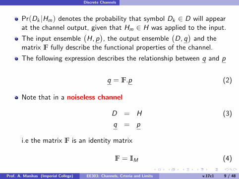
Pr(Dk |Hm) denotes the probability that symbol Dk ∈ D will appearat the channel output, given that Hm ∈ H was applied to the input.The input ensemble
(H, p
), the output ensemble
(D, q
)and the
matrix F fully describe the functional properties of the channel.
The following expression describes the relationship between q and p
q = F.p (2)
Note that in a noiseless channel
D = H (3)
q = p
i.e the matrix F is an identity matrix
F = IM (4)
Prof. A. Manikas (Imperial College) EE303: Channels, Crteria and Limits v.17c1 9 / 48

Converting a Continuous to a Discrete Channel
Converting a Continuous to a Discrete ChannelA continuous channel is converted into (becomes) a discrete channelwhen a digital modulator is used to feed the channel and a digitaldemodulator provides the channel output.A digital modulator is described by M different channel symbols .These channel symbols are ENERGY SIGNALS of duration Tcs .Digital Modulator:
Digital Demodulator:
If M = 2 ⇒Binary Digital Modulator ⇒Binary Comm. SystemIf M > 2 ⇒M-ary Digital Modulator ⇒M-ary Comm. System
Prof. A. Manikas (Imperial College) EE303: Channels, Crteria and Limits v.17c1 10 / 48

Converting a Continuous to a Discrete Channel
..01..101..00..
0..00 s t1( )=t
0..01 s t2( )=t
1..11 s tM( )= t
ts t( )=
Tcs
Tcs
Tcs
Tcs
: H ,Pr(H )1 1
: H ,Pr(H )2 2
: H , Pr(H )M M
..00..101..10..
0..00 s t1( )=t
0..01 s t2( )=t
1..11 s tM( )= tt
r t s t t( )= ( )+n( )
Tcs
Tcs
Tcs
Tcs
: D , Pr(D )1 1
: D , Pr(D )2 2
: D , Pr(D )M M
Channel
s t( )
r t( )=Detectorwith a
DecisionDevice
(DecisionRule)
D
Prof. A. Manikas (Imperial College) EE303: Channels, Crteria and Limits v.17c1 11 / 48

More on Discrete Channels Backward transition Matrix
More on Discrete ChannelsBackward transition Matrix
There are also occassions where we get/observe the output of achannel and then, based on this knowledge, we refer to the input .
In this case we may use the concept of an imaginary "backward "channel and its associated transition matrix, known as backwardtransition matrix defined as follows:
B =
Pr(H1|D1), Pr(H1|D2), ..., Pr(H1|DK )Pr(H2|D1), Pr(H2|D2), ..., Pr(H2|DK )
..., ..., ..., ...Pr(HM |D1), Pr(HM |D2), ..., Pr(HM |DK )
T
(5)
Prof. A. Manikas (Imperial College) EE303: Channels, Crteria and Limits v.17c1 12 / 48

More on Discrete Channels Joint transition Probability Matrix
Joint transition Probability MatrixThe joint probabilistic relationship betweeninput channel symbols H = {H1,H2, ...,HM} and output channelsymbols D = {D1,D2, ...,DM},is described by the so-called joint-probability matrix,
J ,
Pr(H1,D1), Pr(H1,D2), ..., Pr(H1,DK )Pr(H2,D1), Pr(H2,D2), ..., Pr(H2,DK )
..., ..., ..., ...Pr(HM ,D1), Pr(HM ,D2), ..., Pr(HM ,DK )
T
(6)
J is related to the forward transition probabilities of a channel withthe following expression (compact form of Bayes’Theorem):
J = F.
p1 0 ... 00 p2 ... 0... ... ... ...0 0 ... pM
︸ ︷︷ ︸
,diag(p)
= F.diag(p) (7)
Prof. A. Manikas (Imperial College) EE303: Channels, Crteria and Limits v.17c1 13 / 48

More on Discrete Channels Joint transition Probability Matrix
Note: This is equivalent to a new (joint) source having alphabet
{(H1,D1) , (H1,D2) , ..., (HM ,DK )}
and ensemble (joint ensemble) defined as follows
(H ×D, J) =
(H1,D1),Pr(H1,D1)(H1,D2),Pr(H1,D2)
...(Hm ,Dk ),Pr(Hm ,Dk )
...(HM ,DK ),Pr(HM ,DK )
(8)
=
(Hm ,Dk ),Pr(Hm ,Dk )︸ ︷︷ ︸
=Jkm
, ∀mk : 1 ≤ m ≤ M, 1 ≤ k ≤ K
Prof. A. Manikas (Imperial College) EE303: Channels, Crteria and Limits v.17c1 14 / 48

Measure of Information at the Output of a Channel
Measure of Information at the Output of a Channel
In general three measures of information are of main interest:
1 the Entropy of a Source - in (info) bits per source symbol
2 the Mutual Entropy (or Multual Information) of a Channel , in(info) bits per channel symbol
3 the Discrimination of a Sink
Next we will focus on the Mutual Information of a Channel Hmut
Prof. A. Manikas (Imperial College) EE303: Channels, Crteria and Limits v.17c1 15 / 48

Measure of Information at the Output of a Channel Mutual Information of a Channel
Mutual Information of a Channel
The mutual information measures the amount of information thatthe output of the channel (i.e. received message) gives aboutthe input to the channel (transmitted message).
That is, when symbols or signals are transmitted over a noisycommunication channel, information is received. The amount ofinformation received is given by the mutual information,
Hmut = 0 (9)
Prof. A. Manikas (Imperial College) EE303: Channels, Crteria and Limits v.17c1 16 / 48

Measure of Information at the Output of a Channel Mutual Information of a Channel
Hmut , Hmut (p,F) = −M
∑m=1
K
∑k=1
Fkm .pm log2
(qkFkm
)(10)
= −M
∑m=1
K
∑k=1
Jkm log2
(pm .qkJkm
)(11)
= −1TK
J� log2[(
F.p.pT)∅J]
︸ ︷︷ ︸K×M matrix
1M bitssymbol
(12)
where
1M = a column vector of M ones
�,∅ = Hadamard operators (mult. and div.)
Note that1TA1 = adds all elements of A (13)
Prof. A. Manikas (Imperial College) EE303: Channels, Crteria and Limits v.17c1 17 / 48

Measure of Information at the Output of a Channel Equivocation & Mutual Information of a Discrete Channel
Equivocation & Mutual Information of a Discrete ChannelConsider a discrete source (H, p) followed by a discrete channel, asshown belowThe average amount of information gained (or uncertaintyremoved) about the H source (channel input) by observing theoutcome of the D source (channel output), is given by the conditionalentropy HH |D which is defined as follows:
HH |D , HH |D (J) = −M
∑m=1
K
∑k=1
Jkm . log2
(Jkmqk
)(14)
= −1TK
J� log2
B︷ ︸︸ ︷
diag (q)−1 J
︸ ︷︷ ︸
K×M matrix
1Mbits
symbol
(15)
Prof. A. Manikas (Imperial College) EE303: Channels, Crteria and Limits v.17c1 18 / 48

Measure of Information at the Output of a Channel Equivocation & Mutual Information of a Discrete Channel
A similar expression can be also given for the average informationgained about the channel output D by observing the channel input H,i.e.
HD |H , HD |H (J) = −M
∑m=1
K
∑k=1
Jkm . log2
(Jkmpm
)(16)
= −1TK
J� log2
F︷ ︸︸ ︷
J.diag (p)−1
︸ ︷︷ ︸
K×M matrix
1Mbits
symbol
(17)
The conditional entropy HH |D is also known as equivocation and itis the entropy of the noise or, otherwise, the uncertainty in theinput of the channel from the receiver’s point of view.
Prof. A. Manikas (Imperial College) EE303: Channels, Crteria and Limits v.17c1 19 / 48

Measure of Information at the Output of a Channel Equivocation & Mutual Information of a Discrete Channel
Notes1 for a noiseless channel:
HH |D = 0 (18)2 For a discrete memoryless channel,
Hmut , Hmut (p,F) = HH −HH |D (19)
= HD −HD |H (20)
Prof. A. Manikas (Imperial College) EE303: Channels, Crteria and Limits v.17c1 20 / 48

Capacity of a Channel Shannos’s Capacity Theorem
Capacity of a ChannelShannon’s Capacity Theorem
There is a theoretical upper limit to the performance of a specifieddigital communication system with the upper limit depending on theactual system specified.
However, in addition to the specific upper limit associated with eachsystem, there is an overall upper limit to the performance which nodigital communication system, and in fact no communication systemat all, can exceed.
This bound (limit) is important since it provides the performance levelagainst which all other systems can be compared.
The closer a system comes, performance wise, to the upper limit thebetter.
Prof. A. Manikas (Imperial College) EE303: Channels, Crteria and Limits v.17c1 21 / 48

Capacity of a Channel Shannos’s Capacity Theorem
The theoretical upper limit was given by Shannon (1948) as an upperbound to the maximum rate at which information can be transmittedover a communication channel.This rate is called channel capacity and is denoted by the symbol C .Shannon’s capacity theorem states:
C , max (Hmut ) bitssymbol (21)
or
C , rcs ×max (Hmut ) bitssec (22)
where rcs denotes the channel-symbol rate (in channel-symbols persec) with
rcs =1Tcs
(23)
B ≥ rcs2
(24)
i.e. if Hmut (p,F) is maximised with respect to the input probabilitiesp, then it becomes equal to C , the channel capacity (in bits/symbol)
Prof. A. Manikas (Imperial College) EE303: Channels, Crteria and Limits v.17c1 22 / 48

Capacity of a Channel Capacity of AWGN Channels
Capacity of AWGN Channels
In the case of a continuous channel corrupted by additive whiteGaussian noise the capacity is given by
C =12log2 (1+ SNRin)
bitssymbol (25)
or (26)
C = B log2 (1+ SNRin)bitssec (27)
where
B = baseband band width of channel
SNRin =PsPn
Ps = Power of the signal at point T
Pn = Power of the noise at point T = N0B
Prof. A. Manikas (Imperial College) EE303: Channels, Crteria and Limits v.17c1 23 / 48

Capacity of a Channel Capacity of non-Gaussian Channels
Capacity of non-Gaussian ChannelsIf the pdf of the noise is arbitrary (non-Gaussian) then it is verydiffi cult to estimate the capacity .
However, it can be proved [Shannon 1948] that in this case thecapacity is bounded as follows:
B log2
(Ps +NnNn
)≤ C ≤ B log2
(Ps + PnNn
)bitssec (28)
where
Ps : is the average received signal power,
Nn : is the entropy power of the noise, and
Pn : is the power of the noise
Equation 28 is important in that it can be used to provide bounds forany kind of channel.
Prof. A. Manikas (Imperial College) EE303: Channels, Crteria and Limits v.17c1 24 / 48

Capacity of a ChannelShannon’s Channel Capacity Theorem based on Continuous
Channel Parameters
Shannon’s Channel Capacity Theorem based onContinuous Channel Parameters
Consider a time-continuous channel which comprises of a linear timeinvariant filter with transfer function H(f ), the output of which iscorrupted by an additive zero mean stationary noise n(t) of PSDn(f ).
I if the average power of the channel input signal is constraint to be Ps ,then
Ps =
∞∫−∞
max
{0, θ − PSDn(f )
|H(f )|2
}.df (29)
and C ≥∞∫−∞
max
{0,12log2
(θ. |H(f )|2
PSDn(f )
)}.df (30)
with the equality holding if the noise is Gaussian.I Further, if the channel noise is white Gaussian with PSDn(f ) =
N02
then Equation 30 simplifies to the well known result
C = B log2 (1+ SNRin)bitssec (31)
Prof. A. Manikas (Imperial College) EE303: Channels, Crteria and Limits v.17c1 25 / 48

Bandwidth and Channel Symbol Rate
Bandwidth and Channel Symbol Rate
The following expression are given without any proof:
Baseband Bandwidth ≥ channel symbol rate2
(32)
Bandpass Bandwidth ≥ channel symbol rate2
× 2 (33)
The equality is known as Nyquist Bandwidth.In this course, except if it is defined otherwise,
I the word "bandwidth" will mean "Nyquist bandwidth"I the carrier will be ignored and thus "bandwidth" by default will refer to"baseband bandwdith"
Prof. A. Manikas (Imperial College) EE303: Channels, Crteria and Limits v.17c1 26 / 48

Criteria and Limits Introduction
Criteria and Limits of DCSIntroduction
Digital Communications provide excellent message-reproduction andgreatest Energy (EUE) and Bandwidth (BUE) Utilization Effi ciencythrough effective employment of two fundamental techniques:
I source compression coding (to reduce the transmission rate for agiven degree of fidelity)
I error control coding and digital modulation (to reduce the SNRand bandwidth requirements)
With reference to the general structure of a DCS given in the nextpage,
I the source compression coding is implemented by the blocks "SourceEncoder" and "Source Decoder"
I the error control coding is implemended by the "Discrete ChannelEndoder", "Interleaver", "DeInterleaver" and "Discrete ChannelDecoder".
Prof. A. Manikas (Imperial College) EE303: Channels, Crteria and Limits v.17c1 27 / 48

Criteria and Limits Introduction
Prof. A. Manikas (Imperial College) EE303: Channels, Crteria and Limits v.17c1 28 / 48
Criteria and Limits Introduction
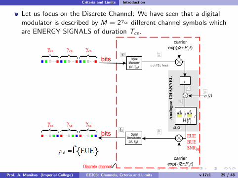
Let us focus on the Discrete Channel: We have seen that a digitalmodulator is described by M = 2γcs different channel symbols whichare ENERGY SIGNALS of duration Tcs .
Prof. A. Manikas (Imperial College) EE303: Channels, Crteria and Limits v.17c1 29 / 48

Criteria and Limits Energy Utilisation Effi ciency (EUE)
Energy Utilisation Effi ciency (EUE)The parameter EUE is a measure of how effi ciently the system utilisesthe available energy in order to transmit information in the presenceof additive white Gaussian noise of double-sided power spectraldensity PSDn(f ) = N0/2 and it is defined as follows:
EUE , EbN0
(34)
Note that EUE is directly related to the received signal power. It willbe appreciated of course that this is, in turn, directly related to thetransmitted power by the attenuation factor introduced by thechannel.Clearly, a question of major importance is how large EUE needs tobe in order to achieve communication at some specific bit errorprobability pe .Obviously the smaller EUE to achieve a specified error probabilitythe better .
Prof. A. Manikas (Imperial College) EE303: Channels, Crteria and Limits v.17c1 30 / 48

Criteria and Limits Bandwidth Utilisation Effi ciency (BUE)
Bandwidth Utilisation Effi ciency (BUE)
The BUE measures how effi ciently the system utilises the bandwidthB available to send information and it is defined as follows:
BUE , Brb
(35)
where rb denotes the bit rate.
Specifically, the BUE indicates how much bandwidth is beingused per transmitted information bit and hence, for a given levelof performance, the smaller BUE the better since this means thatless bandwidth is being used to achieve a given rate of datatransmission.
N.B.:signaling speed , rb
B= BUE−1 (36)
Prof. A. Manikas (Imperial College) EE303: Channels, Crteria and Limits v.17c1 31 / 48

Criteria and Limits Visual Comparison of Comm Systems
Visual Comparison of Comm SystemsBy using EUE and BUE the SNRin can be expressed as follows
SNRin = PsPn=
EbTb
N0B= Eb
N0BTb= Eb
N0B 1rb=
EbN0Brb
= EUEBUE (37)
By determining the EUE and BUE of any particular system, thatsystem can be represented as a point in the plane (EUE,BUE).It is desirable for this point to be as close to the origin as possible
C = B log2(1+ EUE
BUE
) bitssec (38)
C/B = log2(1+ EUE
BUE
) bitssecHz (39)
Prof. A. Manikas (Imperial College) EE303: Channels, Crteria and Limits v.17c1 32 / 48

Criteria and Limits Visual Comparison of Comm Systems
N.B.:I a line from origin represents those points (systems) in the plane forwhich the SNRin=constant
I By comparing points representing one system with those representinganother ⇒ VISUAL COMPARISON !
I It can be observed that
F CS1 beter than CS2 which is better than CS3F CS2 and CS3 have the same SNRin
Prof. A. Manikas (Imperial College) EE303: Channels, Crteria and Limits v.17c1 33 / 48

Criteria and Limits Theoretical Limits
Theoretical Limits
We have seen that the capacity of a white Gaussian channel ofbandwidth B is
C = B log2 (1+ SNRin)bitssec (40)
Please don’t forget that the above equation refers to bandlimitedwhite-noise channel with a constraint on the average transmittedpower.
Question: if B =↑ (and in particluar if B = ∞) then C =?Answer :
I From the capacity-equation (Equ 40) it can be seen that B ↑=⇒ C ↑I However, when B tends to ∞ then
C∞ = 1.44PsN0
(41)
Prof. A. Manikas (Imperial College) EE303: Channels, Crteria and Limits v.17c1 34 / 48

Criteria and Limits Theoretical Limits
Prof. A. Manikas (Imperial College) EE303: Channels, Crteria and Limits v.17c1 35 / 48

Criteria and Limits Theoretical Limits
LIMIT-1 : limit on bit rateI when binary information is transmitted in the channel, rb should belimited as follows:
rb ≤ C (42)
I ideal case:rb = C (43)
LIMIT-2 : limit on EUEI the best Energy Effi ciency is EUE=0.693. This is the ultimate limitbelow which no physical channel can transmit without errorsi.e
EUE ≥ 0.693
LIMIT-3 : Shannon’s threshold channel capacity curve
I This is the curve EUE=f{BUE} for a bit rate rb equal to its maximumvalue,i.e.
rb = C ⇒ EUE =2BUE − 1BUE−1
(44)
Prof. A. Manikas (Imperial College) EE303: Channels, Crteria and Limits v.17c1 36 / 48

Criteria and Limits Theoretical Limits
Plot of Equation 44:
No physical realizable CS could occupy a point in the plane(EUE,BUE) lying below this theoretical channel capacity curve .
Prof. A. Manikas (Imperial College) EE303: Channels, Crteria and Limits v.17c1 37 / 48

Criteria and Limits Theoretical Limits
SNRin =EUEdataBUEdata
=EUEinfBUEinf
(45)
data rate : rb ,data = rcs × log2M (46)
info rate : rb ,info = rcs ×Hmut (47)
Prof. A. Manikas (Imperial College) EE303: Channels, Crteria and Limits v.17c1 38 / 48

Criteria and Limits Theoretical Limits
Point B always should be above the Shannon’s thr. capacity curve.
Point A may be above or below the Shannon’s thr. capacity curve.The following table gives the corresponding equivalent parametersbetween Analogue and Digital Comm Systems which can be used toplace on the (EUE,BUE) not only digital but also analoguecommunication systems
Digital CS Analogue CS
EUE= EbN0= Ps
N0rb⇔ SNRin-mb =
PsN0.Fg
rb ⇔ FgBUE= B
rb⇔ β , B
Fg
where:I Fg denotes the maximum frequency of the message signal g(t), i.e. itrepresents the bandwidth of the message
I β is known as "bandwidth expansion factor",e.g. SSB: β = 1;AM: β = 2
Prof. A. Manikas (Imperial College) EE303: Channels, Crteria and Limits v.17c1 39 / 48
Criteria and Limits Theoretical Limits
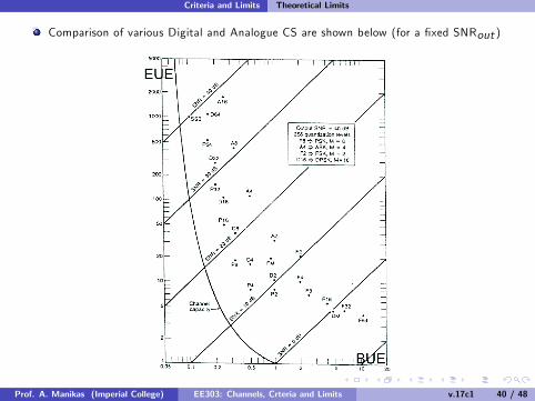
Comparison of various Digital and Analogue CS are shown below (for a fixed SNRout )
Prof. A. Manikas (Imperial College) EE303: Channels, Crteria and Limits v.17c1 40 / 48

Other Comparison-Parameters
Other Comparison-Parameters
SPECTRAL CHARACTERISTICS of transmitted signal(rate at which spectrum falls off).
INTERFERENCE RESISTANCEI it may be necessary to increase (EUE,BUE) in order to increase interf.resistance
FADINGI Fading problem pe =↑I Note that, if
{BUE =↑EUE =↓
}then Fading=↓
DELAY DISTORTIONI Try to avoid this problem by selecting appropriate signals
COST and COMPLEXITY
Prof. A. Manikas (Imperial College) EE303: Channels, Crteria and Limits v.17c1 41 / 48

Appendix-A: SNR at the output of an Ideal Comm System
Appendix: SNR at the output of an Ideal Comm System
In this section a so-called ideal system of communication will beconsidered and it will be shown that bandwidth can be exchanged forsignal-to-noise performance.
The ideal system forms a benchmark against which othercommunication systems can be compared.
An ideal system has been defined as one that transmits data at a bitrate
r = C (48)
where C is the channel capacity i.e. C = B log2 (1+ SNRin) bits/sec
Prof. A. Manikas (Imperial College) EE303: Channels, Crteria and Limits v.17c1 42 / 48

Appendix-A: SNR at the output of an Ideal Comm System
Furthermore we have seen that for an ideal communication system:
EUE =SNRin
log2(1+ SNRin)⇒ lim
SNRin→0EUE = 0.693 (49)
BUE =1
log2(1+EUEBUE )
(50)
⇒ EUE =2BUE
−1 − 1BUE−1
⇒ limBUE→∞
EUE = 0.693 (51)
Prof. A. Manikas (Imperial College) EE303: Channels, Crteria and Limits v.17c1 43 / 48

Appendix-A: SNR at the output of an Ideal Comm System
Block Diagram of an Ideal Communication System:
Prof. A. Manikas (Imperial College) EE303: Channels, Crteria and Limits v.17c1 44 / 48

Appendix-A: SNR at the output of an Ideal Comm System
The previous figure shows the elements of a basic idealcommunication system.
An input analogue message signal g(t), which is of bandwidth Fg , isapplied to a signal mapping unit which, in response to g(t), producesan analogue signal s(t) of bandwidth B and this signal is transmittedover an analogue channel having a similar bandwidth, B.
I The channel is corrupted by additive white Gaussian noise of doublesided power spectral density N0/2 which is bandlimited to the channelbandwidth B.
I Let the signal-to-noise ratio at the input of the receiver be SNRin .I Assume further that the received signal, plus noise, is then fed to adetector having a bandwidth Fg , equal to the message bandwidth.
I Let the signal-to-noise ratio at the output of the detector be SNRout.
Prof. A. Manikas (Imperial College) EE303: Channels, Crteria and Limits v.17c1 45 / 48

Appendix-A: SNR at the output of an Ideal Comm System
Now the capacity of the analogue transmission system (channel) is
C = B log2 (1+ SNRin) bits/s (52)
Also, the "mapping-unit/channel/detector" can be regarded as achannel having a signal-to-noise ratio SNRout and hence it too canbe regarded as an AWGN channel and its capacity is given by
C ′ = Fg log2 (1+ SNRout ) bits/s (53)
If, in order to avoid information loss (ideal case), the capacities areset equal then it can be seen, after simple mathematicalmanipulation, that
C ′ = C ⇒ ...⇒ SNRout ,ideal = (1+ SNRin)BFg − 1 (54)
= (1+SNRin−mb
β)β − 1 (55)
where β is the bandwidth expansion factor.
Prof. A. Manikas (Imperial College) EE303: Channels, Crteria and Limits v.17c1 46 / 48

Appendix-A: SNR at the output of an Ideal Comm System
The above expression is fundamentally important since it shows thatthe overall system performance, SNRout , can be improved by usingmore channel bandwidth.The figure below shows, as a function of the bandwidth expansionfactor β, typical curves of SNRout versus SNRin−mb for the idealcommunication system.
Note that all other known communication systems should becompared with this optimum performance provided by Equation .
Prof. A. Manikas (Imperial College) EE303: Channels, Crteria and Limits v.17c1 47 / 48

Appendix-A: SNR at the output of an Ideal Comm System
From the previous figure it can be seen that:I if SNRin−mb is small then on increasing β the effect on the SNRout issmall (i.e. very little increase in the SNRout is obtained).
I If, however, SNRin−mb is large then a small increase in the bandwidthexpansion factor results in a large increase in the SNRout .
I A practical consequence of this is that if the SNRin−mb is small thenthere is little to be gained from using more channel bandwidth.
Case-1:SNRin-mb=small Case-2:SNRin-mb=large=10SNRin-mb=1 SNRin-mb=10
β = 1 SNRout=1 SNRout=10
β = 2 SNRout=1.25 SNRout=35
β = 100 SNRout=1.7048 SNRout=13780
Prof. A. Manikas (Imperial College) EE303: Channels, Crteria and Limits v.17c1 48 / 48
Related Documents


