EE 418 Lecture 02 - AASTMT

1

Automatic Control EE 418 “Dr. Ahmed El-Shenawy”

Automatic Control EE 418

Lecture 2

<Dr Ahmed El-Shenawy>

2


Differential equation of physical systems

Linear Ordinary Differential Equations

A first-order linear ordinary differential equation

Second-order differential equation

3


Nonlinear Differential Equations

Many physical systems are nonlinear and must be described by nonlinear differential equations. For instance, the following differential equation that describes the motion of a pendulum of mass m and length /, later discussed in this chapter, is

Because 6{t) appears as a sine function, Eq. (2-100) is nonlinear, and the system is called a nonlinear system.

4


Modeling of DynamicSystems

One of the most important tasks in the analysis and design of control systems is mathematical modeling of the systems. One of the mostcommon methods of modeling linear systems is the transfer function method.The control systems engineer often has the task of determining not only how to accurately describe a system mathematically but, more importantly, how to make proper assumptions and approximations, whenever necessary, so that the system may be realistically characterized by a linear mathematical model.

A control system may be composed of various components includingmechanical, thermal, fluid, pneumatic, and electrical; sensors and actuators; and computers. In this chapter, we review basic properties of these systems, otherwise known as dynamic systems.

5


The mainobjectives of this Lecture

• To introduce modeling of mechanical systems.

• To introduce modeling of electrical systems.

6


MODELING OF MECHANICAL SYSTEMS

Definition: Mass is considered a property of an element that stores the kinetic energy of translational motion.

Translational Motion

The motion of translation is defined as a motion that takes place along a straight or curved path. The variables that are used to describe translational motion are acceleration, velocity, and displacement.

7



Newton's law of motion states that the algebraic sum of external forces acting on a rigid body in a given direction is equal to the product of the mass of the body and its acceleration in the same direction. The law can be expressed as

where M denotes the mass, and a is the acceleration in the direction considered.

8



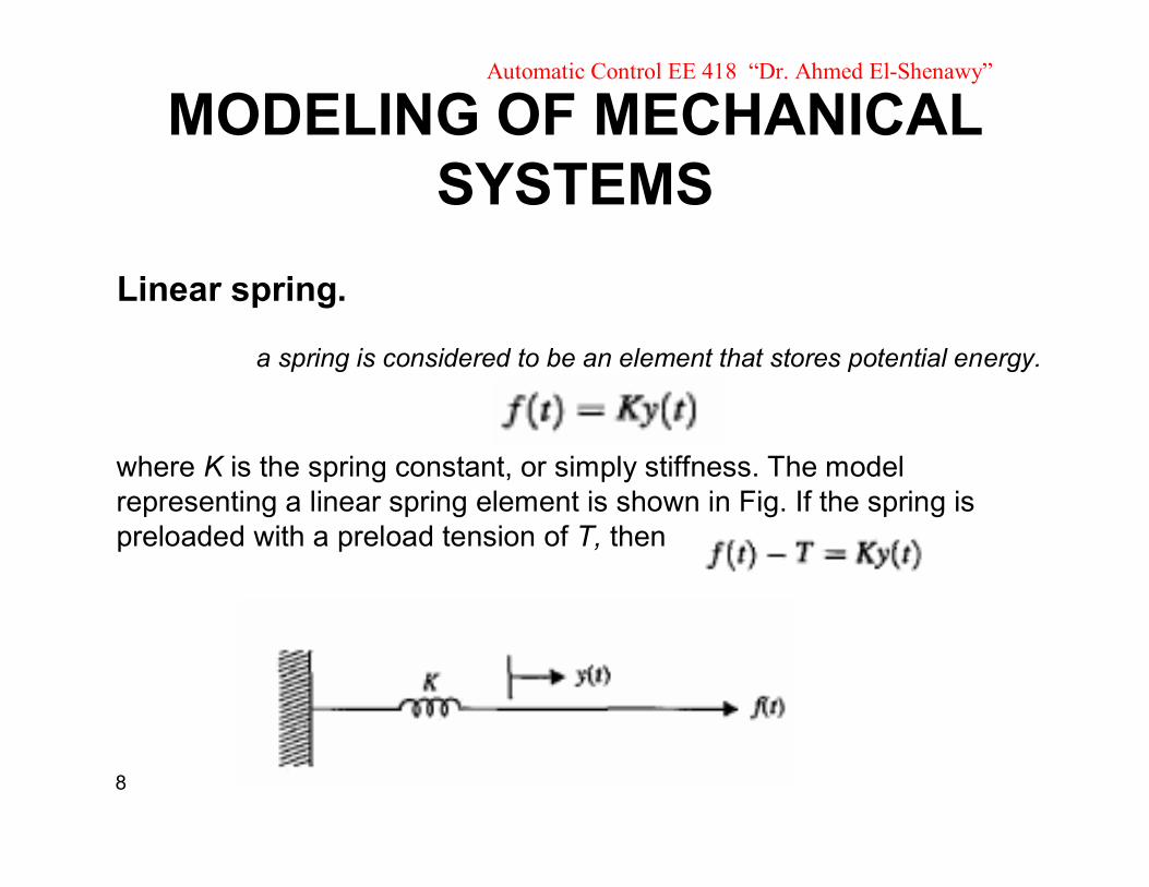
Linear spring.

a spring is considered to be an element that stores potential energy.

where K is the spring constant, or simply stiffness. The model representing a linear spring element is shown in Fig. If the spring is preloaded with a preload tension of T, then

9



Friction for translation motion.

Whenever there is motion or tendency of motion between two physical elements, frictional forces exist.

Three different types of friction are commonly used in practicalsystems: viscous friction, static friction, and Coulomb friction.

Viscous friction. Viscous friction represents a retarding force that is a linear relationship between the applied force and velocity. where B is the viscous frictional coefficient

10



Static friction. Static friction represents a retarding force that tends to preventmotion from beginning

Coulomb friction. Coulomb friction is a retarding force that has constant amplitude with respect to the change of velocity, but the sign of the frictional force changes with the reversal of the direction of velocity.

11



12


EXAMPLE (1)Consider the mass-spring-friction system shown in Fig. 1-a The linear motion concerned is in the horizontal direction. The free-body diagram of the system is shown in Fig. 1-b). The force equation of the system is

13


represent velocity and acceleration, respectively

For zero initial conditions, the transfer function between Y(s) and F(s) is obtained by taking the Laplace transform on both sides

14


15


16


EXAMPLE (2)

consider the system shown in Fig

17


These equations are rearranged in input-output form as

For zero initial conditions, the transfer function between Y\(s) and Y2(s) is obtained by taking the Laplace transform on both sides

18


Rotational Motion

The rotational motion of a body can be defined as motion about a fixed axis. The extension of Newton's law of motion for rotational motion states that the algebraic sum of moments or torque about a fixed axis is equal to the product of the inertia and the angular acceleration about the axis. Or

where J denotes the inertia and a is the angular acceleration.

The other variables generally used to describe the motion of rotation are torque , angular velocity , and angular displacement . The elements involved with the rotational motion

19


Inertia. Inertia, J,

The inertia of a given element depends on the geometric composition about the axis of rotation and its density

Torsional spring.As with the linear spring for translational motion, a torsional spring constant K, in torque-per-unit angular displacement, can be devised to represent the compliance of a rod or a shaft when it is subject to an applied torque.

20


Friction for rotational motion.

The three types of friction described for translational motion can be carried over to the motion of rotation.

• Viscous friction. Static friction. Coulomb friction.

EXAMPLE (3)

21


EXAMPLE 4

Fig. shows the diagram of a motor coupled to an inertial load through a shaft with a spring constant K. A non-rigid coupling between two mechanical components in a control system often causes torsional resonances that can be transmitted to all parts of the system. The system variables and parameters are defined as follows:

22


Gear Trains

23


MODELING OF SIMPLE ELECTRICAL SYSTEMS

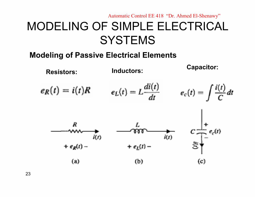
Modeling of Passive Electrical Elements

Resistors: Inductors: Capacitor:

24


Modeling of Electrical Networks

EXAMPLE(4)

25


EXAMPLE (5)

26


MODELING OF ACTIVE ELECTRICAL ELEMENTS:

OPERATIONAL AMPLIFIERSOperational amplifiers, or simply op-amps, offer a convenient way to build, implement, or realize continuous-data or s-domain transfer functions. In control systems, op-amps are often used to implement the controllers or compensatorsthat evolve from the control system design process, so in this section we illustrate common op-amp configurations.

27

Automatic Control EE 418 “Dr. Ahmed El-Shenawy”Sums and Differences

28


29


Mathematical Modeling of PM DC Motors

Dc motors are extensively used in control systems. In this section we establish the mathematical model for dc motors. As it will be demonstrated here, the mathematical model of a dc motor is linear

30



The armature is modeled as a circuit with resistance Ra connected in series with an inductance La, and a voltage source eb, representing the back emfelectromotive force) in the armature when the rotor rotates

31



The motor variables and parameters are defined as follows:

32


where 7/,(0 represents a load frictional torque such as Coulomb friction.

33


EE 418 Lecture 02 - AASTMT

Documents