Econ 240 C Econ 240 C Lecture 14 Lecture 14 1

Econ 240 C Lecture 14 1. 2 Project II I. Work in Groups II. You will be graded based on a PowerPoint presentation and a written report. III. Your report.
Dec 19, 2015
Welcome message from author
This document is posted to help you gain knowledge. Please leave a comment to let me know what you think about it! Share it to your friends and learn new things together.
Transcript

Econ 240 CEcon 240 C
Lecture 14Lecture 14
1

2
Project IIProject II

I. Work in GroupsII. You will be graded based on a PowerPoint presentation and a written report.III. Your report should have an executive summary of one to one and a half pages that summarizes your findings in words for a non-technical reader. It should explain the problem being examined from an economic perspective, i.e. it should motivate interest in the issue on the part of the reader. Your report should explain how you are investigating the issue, in simple language. It should explain why you are approaching the problem in this particular fashion. Your executive report should explain the economic importance of your findings.

4
Technical Appendix1. Table of Contents2. Spreadsheet of data used and sources or, if extensive, a subsample of the data3. Describe the analytical time series techniques you are using4. Show descriptive statistics and histograms for the variables in the study5. Use time series data for your project; show a plot of each variable against time
The technical details of your findings you can attach as an appendix

5
Group A Group BGroup C
Tara Copello Pungdalis Suos Calvin YeungZhimin Zhou Micah Witt Andrew CahillAndrea Cardani Charles Rabkin Ashley HedbergJonathan Hester Will Hippen Jesse SmithEvan Nakano Thomas Bruister Darren DoiEric Laschinger Arnaud Piechaud Sarab KhalsaYana Ten Kyu-Sang Park Jong Duk Woo
Group D Group E
Carl-Einar Thorner Jeffrey AhlvinRobert Connor Gleason Russell LudwickAntung Anthony Liu Aren MegerdichianHamid Ghofrani Carrie KoenJoonho Shin Anthony KaszaUfook Sahilliohlu Matthew Stevens
6
OutlineOutline
Exponential SmoothingExponential SmoothingBack of the envelope formula: geometric Back of the envelope formula: geometric
distributed lag: L(t) = a*y(t-1) + (1-a)*L(t-1); distributed lag: L(t) = a*y(t-1) + (1-a)*L(t-1); F(t) = L(t)F(t) = L(t)
ARIMA (p,d,q) = (0,1,1); ARIMA (p,d,q) = (0,1,1); ∆y(t) = e(t) –(1-a)e(t-∆y(t) = e(t) –(1-a)e(t-1)1)
Error correction: L(t) =L(t-1) + a*e(t)Error correction: L(t) =L(t-1) + a*e(t) Intervention AnalysisIntervention Analysis

7
Part I: Exponential SmoothingPart I: Exponential Smoothing
Exponential smoothing is a technique Exponential smoothing is a technique that is useful for forecasting short that is useful for forecasting short time series where there may not be time series where there may not be enough observations to estimate a enough observations to estimate a Box-Jenkins modelBox-Jenkins model
Exponential smoothing can be Exponential smoothing can be understood from many perspectives; understood from many perspectives; one perspective is a formula that one perspective is a formula that could be calculated by handcould be calculated by hand
8
0
200
400
600
800
1000
1970 1980 1990 2000 2010
YEAR
HS
EP
RC
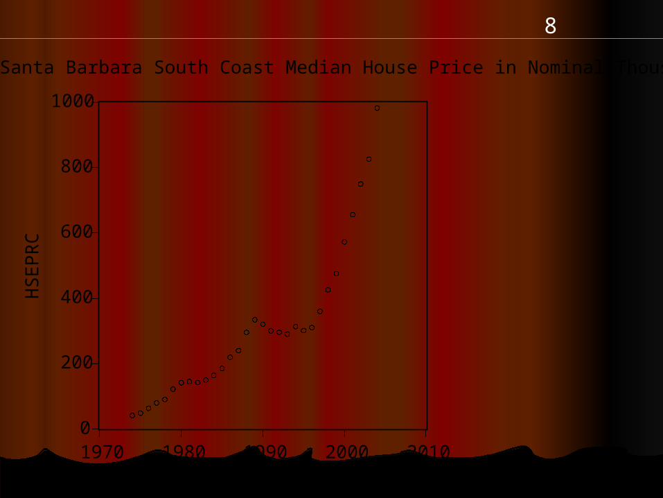
Santa Barbara South Coast Median House Price in Nominal Thousands

9
3
4
5
6
7
1970 1980 1990 2000 2010
YEAR
LN
HS
EP
RC
Three Rates of Growth

10
0
200
400
600
800
1000
1970 1980 1990 2000 2010
YEAR
HS
EP
RC
04
Santa Barbara South Coast House Price, 000 04 $

11Simple exponential Simple exponential smoothingsmoothing
Simple exponential smoothing, also Simple exponential smoothing, also known as single exponential smoothing, known as single exponential smoothing, is most appropriate for a time series is most appropriate for a time series that is a random walk with first order that is a random walk with first order moving average error structuremoving average error structure
The levels term, L(t), is a weighted The levels term, L(t), is a weighted average of the observation lagged one, average of the observation lagged one, y(t-1) plus the previous levels, L(t-1):y(t-1) plus the previous levels, L(t-1):
L(t) = a*y(t-1) + (1-a)*L(t-1)L(t) = a*y(t-1) + (1-a)*L(t-1)

12
Single exponential smoothingSingle exponential smoothing
The parameter a is chosen to minimize The parameter a is chosen to minimize the sum of squared errors where the the sum of squared errors where the error is the difference between the error is the difference between the observation and the levels term: e(t) = observation and the levels term: e(t) = y(t) – L(t)y(t) – L(t)
The forecast for period t+1 is given by The forecast for period t+1 is given by the formula: L(t+1) = a*y(t) + (1-a)*L(t)the formula: L(t+1) = a*y(t) + (1-a)*L(t)
Example from John Heinke and Arthur Example from John Heinke and Arthur Reitsch, Reitsch, Business Forecasting, 6Business Forecasting, 6thth Ed. Ed.

13observations Sales
1 500
2 350
3 250
4 400
5 450
6 350
7 200
8 300
9 350
10 200
11 150
12 400
13 550
14 350
15 250
16 550
17 550
18 400
19 350
20 600
21 750
22 500
23 400
24 650

14
Single exponential smoothingSingle exponential smoothing
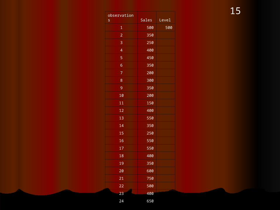
For observation #1, set L(1) = For observation #1, set L(1) = Sales(1) = 500, as an initial conditionSales(1) = 500, as an initial condition
As a trial value use a = 0.1As a trial value use a = 0.1So L(2) = 0.1*Sales(1) + 0.9*Level(1) So L(2) = 0.1*Sales(1) + 0.9*Level(1)
L(2) = 0.1*500 + 0.9*500 = 500 L(2) = 0.1*500 + 0.9*500 = 500And L(3) = 0.1*Sales(2) + And L(3) = 0.1*Sales(2) +
0.9*Level(2) L(3) = 0.1*350 + 0.9*Level(2) L(3) = 0.1*350 + 0.9*500 = 4850.9*500 = 485
15observations Sales Level
1 500 500
2 350
3 250
4 400
5 450
6 350
7 200
8 300
9 350
10 200
11 150
12 400
13 550
14 350
15 250
16 550
17 550
18 400
19 350
20 600
21 750
22 500
23 400
24 650

16observations Sales Level
1 500 500
2 350 500
3 250 485
4 400
5 450
6 350
7 200
8 300
9 350
10 200
11 150
12 400
13 550
14 350
15 250
16 550
17 550
18 400
19 350
20 600
21 750
22 500
23 400
24 650
a = 0.1

17
Single exponential smoothingSingle exponential smoothing
So the formula can be used to So the formula can be used to calculate the rest of the levels calculate the rest of the levels values, observation #4-#24values, observation #4-#24
This can be set up on a spread-sheetThis can be set up on a spread-sheet

18observations Sales Level
1 500 500
2 350 500
3 250 485
4 400 461.5
5 450 455.4
6 350 454.8
7 200 444.3
8 300 419.9
9 350 407.9
10 200 402.1
11 150 381.9
12 400 358.7
13 550 362.8
14 350 381.6
15 250 378.4
16 550 365.6
17 550 384.0
18 400 400.6
19 350 400.5
20 600 395.5
21 750 415.9
22 500 449.3
23 400 454.4
24 650 449.0
a = 0.1
19
Single exponential smoothingSingle exponential smoothing
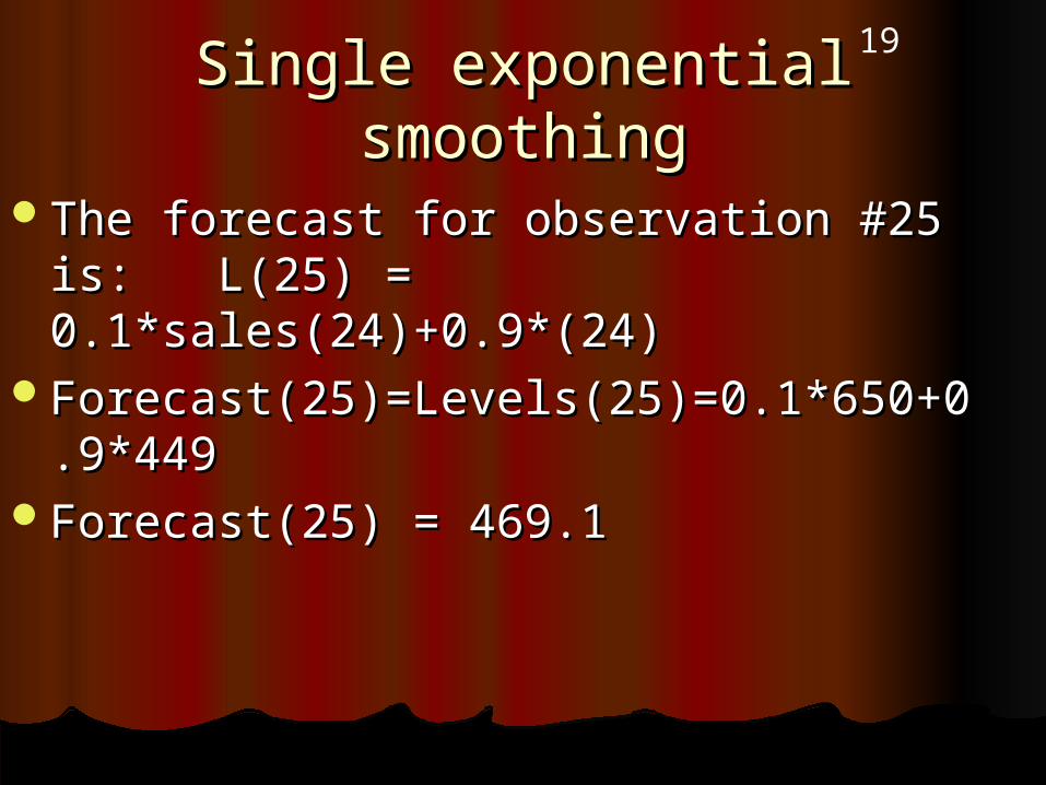
The forecast for observation #25 is: The forecast for observation #25 is: L(25) = 0.1*sales(24)+0.9*(24)L(25) = 0.1*sales(24)+0.9*(24)
Forecast(25)=Levels(25)=0.1*650+0.9Forecast(25)=Levels(25)=0.1*650+0.9*449*449
Forecast(25) = 469.1Forecast(25) = 469.1

Single Exponential Smoothing
0
100
200
300
400
500
600
700
800
1 2 3 4 5 6 7 8 9 10 11 12 13 14 15 16 17 18 19 20 21 22 23 24
Observation
Val
ue Sales
Levels

21Single exponential Single exponential distributiondistribution
The errors can now be calculated: The errors can now be calculated: e(t) = sales(t) – levels(t) e(t) = sales(t) – levels(t)

22observations Sales Level error
1 500 500 0
2 350 500 -150
3 250 485 -235
4 400 461.5 -61.5
5 450 455.4 -5.35
6 350 454.8 -104.8
7 200 444.3 -244.3
8 300 419.9 -119.9
9 350 407.9 -57.9
10 200 402.1 -202.1
11 150 381.9 -231.9
12 400 358.7 41.3
13 550 362.8 187.2
14 350 381.6 -31.6
15 250 378.4 -128.4
16 550 365.6 184.4
17 550 384.0 166.0
18 400 400.6 -0.6
19 350 400.5 -50.5
20 600 395.5 204.5
21 750 415.9 334.1
22 500 449.3 50.7
23 400 454.4 -54.4
24 650 449.0 201.0
a = 0.1
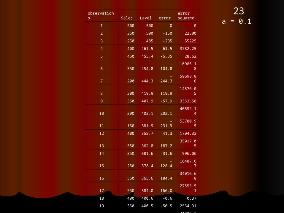
23observations Sales Level error
error squared
1 500 500 0 0
2 350 500 -150 22500
3 250 485 -235 55225
4 400 461.5 -61.5 3782.25
5 450 455.4 -5.35 28.62
6 350 454.8 -104.8 10986.18
7 200 444.3 -244.3 59698.86
8 300 419.9 -119.9 14376.05
9 350 407.9 -57.9 3353.58
10 200 402.1 -202.1 40852.14
11 150 381.9 -231.9 53780.95
12 400 358.7 41.3 1704.33
13 550 362.8 187.2 35027.05
14 350 381.6 -31.6 996.06
15 250 378.4 -128.4 16487.67
16 550 365.6 184.4 34016.68
17 550 384.0 166.0 27553.51
18 400 400.6 -0.6 0.37
19 350 400.5 -50.5 2554.91
20 600 395.5 204.5 41823.74
21 750 415.9 334.1 111594.53
22 500 449.3 50.7 2565.62
23 400 454.4 -54.4 2960.80
24 650 449.0 201.0 40412.28
a = 0.1

24observations Sales Level errorerror squared
1 500 500 0 0
2 350 500 -150 22500
3 250 485 -235 55225
4 400 461.5 -61.5 3782.25
5 450 455.4 -5.35 28.62
6 350 454.8 -104.8 10986.18
7 200 444.3 -244.3 59698.86
8 300 419.9 -119.9 14376.05
9 350 407.9 -57.9 3353.58
10 200 402.1 -202.1 40852.14
11 150 381.9 -231.9 53780.95
12 400 358.7 41.3 1704.33
13 550 362.8 187.2 35027.05
14 350 381.6 -31.6 996.06
15 250 378.4 -128.4 16487.67
16 550 365.6 184.4 34016.68
17 550 384.0 166.0 27553.51
18 400 400.6 -0.6 0.37
19 350 400.5 -50.5 2554.91
20 600 395.5 204.5 41823.74
21 750 415.9 334.1 111594.53
22 500 449.3 50.7 2565.62
23 400 454.4 -54.4 2960.80
24 650 449.0 201.0 40412.28
sum sq res 582281.2
a = 0.1
25
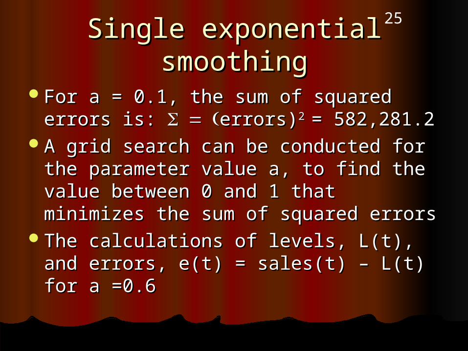
Single exponential smoothingSingle exponential smoothing
For a = 0.1, the sum of squared For a = 0.1, the sum of squared errors is: errors is: errors)errors)2 2 = 582,281.2= 582,281.2
A grid search can be conducted for A grid search can be conducted for the parameter value a, to find the the parameter value a, to find the value between 0 and 1 that value between 0 and 1 that minimizes the sum of squared errorsminimizes the sum of squared errors
The calculations of levels, L(t), and The calculations of levels, L(t), and errors, e(t) = sales(t) – L(t) for a =0.6errors, e(t) = sales(t) – L(t) for a =0.6

26observations Sales Levels
1 500 500
2 350 500
3 250 410
4 400 314
5 450 365.6
6 350 416.2
7 200 376.5
8 300 270.6
9 350 288.2
10 200 325.3
11 150 250.1
12 400 190.0
13 550 316.0
14 350 456.4
15 250 392.6
16 550 307.0
17 550 452.8
18 400 511.1
19 350 444.4
20 600 387.8
21 750 515.1
22 500 656.0
23 400 562.4
24 650 465.0
a = 0.6

27
Single exponential smoothingSingle exponential smoothing
Forecast(25) = Levels(25) = Forecast(25) = Levels(25) = 0.6*sales(24) + 0.4*levels(24) = 0.6*sales(24) + 0.4*levels(24) = 0.6*650 + 0.4*465 = 7760.6*650 + 0.4*465 = 776
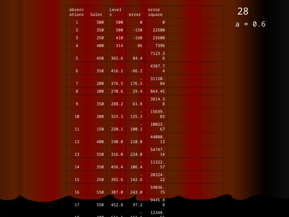
28observations Sales Levels error
error square
1 500 500 0 0
2 350 500 -150 22500
3 250 410 -160 25600
4 400 314 86 7396
5 450 365.6 84.4 7123.36
6 350 416.2 -66.2 4387.74
7 200 376.5 -176.5 31150.84
8 300 270.6 29.4 864.45
9 350 288.2 61.8 3814.38
10 200 325.3 -125.3 15699.02
11 150 250.1 -100.1 10023.67
12 400 190.0 210.0 44080.13
13 550 316.0 234.0 54747.14
14 350 456.4 -106.4 11322.57
15 250 392.6 -142.6 20324.22
16 550 307.0 243.0 59036.75
17 550 452.8 97.2 9445.88
18 400 511.1 -111.1 12348.55
19 350 444.4 -94.4 8920.73
20 600 387.8 212.2 45037.39
21 750 515.1 234.9 55172.40
22 500 656.0 -156.0 24349.97
23 400 562.4 -162.4 26379.58
24 650 465.0 185.0 34237.15
Sum of Sq Res 533961.9
a = 0.6

29
Single exponential smoothingSingle exponential smoothing
Grid search plotGrid search plot

Grid Search for Smoothing Parameter
490000
500000
510000
520000
530000
540000
550000
560000
570000
580000
590000
0 0.2 0.4 0.6 0.8 1 1.2
Smoothing Parameter
Su
m o
f S
qu
ared
Res
idu
als

31
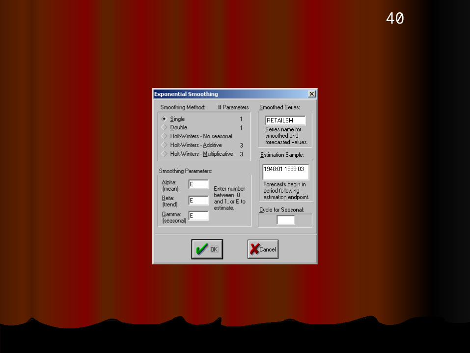
Single Exponential SmoothingSingle Exponential Smoothing EVIEWS: Algorithmic search for the EVIEWS: Algorithmic search for the
smoothing parameter asmoothing parameter a In EVIEWS, select time series sales(t), and In EVIEWS, select time series sales(t), and
openopen In the sales window, go to the PROCS menu and In the sales window, go to the PROCS menu and
select exponential smoothingselect exponential smoothing Select singleSelect single the best parameter a = 0.26 with sum of squared the best parameter a = 0.26 with sum of squared
errors = 472982.1 and root mean square error = errors = 472982.1 and root mean square error = 140.4 = (472982.1/24)140.4 = (472982.1/24)1/21/2
The forecast, or end of period levels mean = 532.4The forecast, or end of period levels mean = 532.4

32

33

34Forecast = L(25) = 0.26*Sales(24) + 0.74L(24) = 532.4=0.26*650 + 0.74*491.07 =532.4

35

36Part II. Three Perspectives on Part II. Three Perspectives on Single Exponential SmoothingSingle Exponential SmoothingThe formula perspectiveThe formula perspective
L(t) = a*y(t-1) + (1 - a)*L(t-1)L(t) = a*y(t-1) + (1 - a)*L(t-1)e(t) = y(t) - L(t)e(t) = y(t) - L(t)
The Box-Jenkins PerspectiveThe Box-Jenkins PerspectiveThe Updating Forecasts PerspectiveThe Updating Forecasts Perspective

37
Box Jenkins PerspectiveBox Jenkins PerspectiveUse the error equation to substitute for L(t) Use the error equation to substitute for L(t)
in the formula, L(t) = a*y(t-1) + (1 - a)*L(t-in the formula, L(t) = a*y(t-1) + (1 - a)*L(t-1)1)L(t) = y(t) - e(t)L(t) = y(t) - e(t)y(t) - e(t) = a*y(t-1) + (1 - a)*[y(t-1) - e(t-1)] y(t) - e(t) = a*y(t-1) + (1 - a)*[y(t-1) - e(t-1)]
y(t) = e(t) + y(t-1) - (1-a)*e(t-1)y(t) = e(t) + y(t-1) - (1-a)*e(t-1)or or y(t) = y(t) - y(t-1) = e(t) - (1-a) e(t-1)y(t) = y(t) - y(t-1) = e(t) - (1-a) e(t-1)
So y(t) is a random walk plus MAONE noise, So y(t) is a random walk plus MAONE noise, i.e y(t) is a (0,1,1) process where (p,d,q) are i.e y(t) is a (0,1,1) process where (p,d,q) are the orders of AR, differencing, and MA.the orders of AR, differencing, and MA.

38
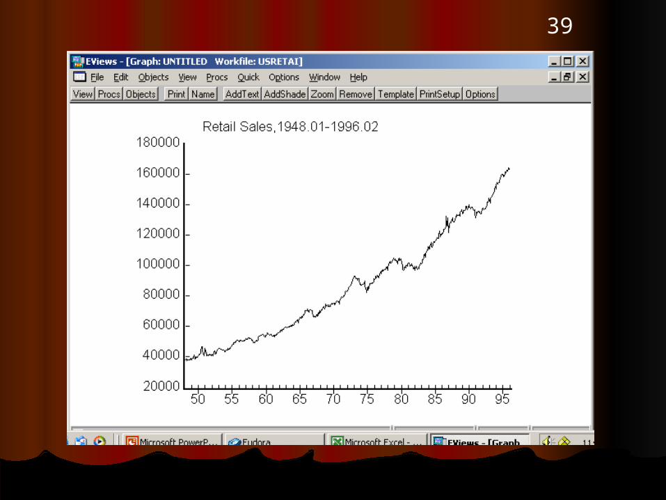
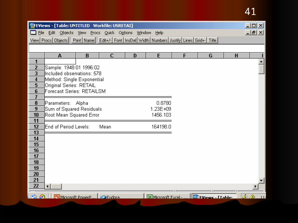
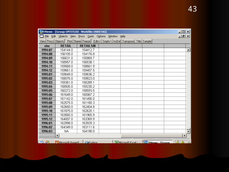
Box-Jenkins PerspectiveBox-Jenkins Perspective
In Lab Eight, we will apply simple In Lab Eight, we will apply simple exponential smoothing to retail sales, exponential smoothing to retail sales, a process you used for forecasting a process you used for forecasting trend in Lab 3, and which can be trend in Lab 3, and which can be modeled as (0,1,1).modeled as (0,1,1).
39
40
41
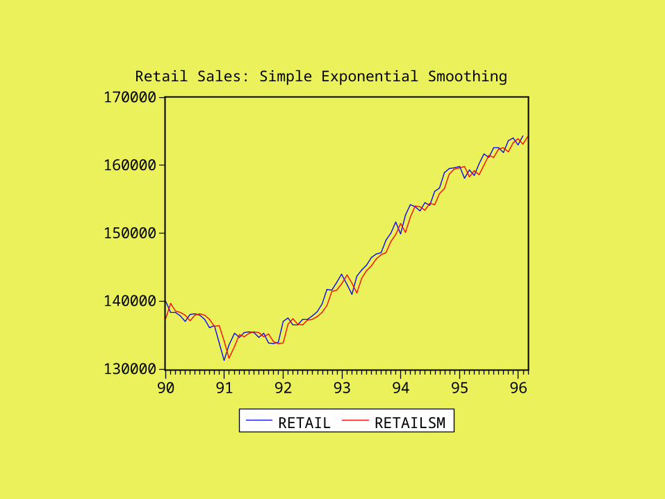
130000
140000
150000
160000
170000
90 91 92 93 94 95 96
RETAIL RETAILSM
Retail Sales: Simple Exponential Smoothing
43
44
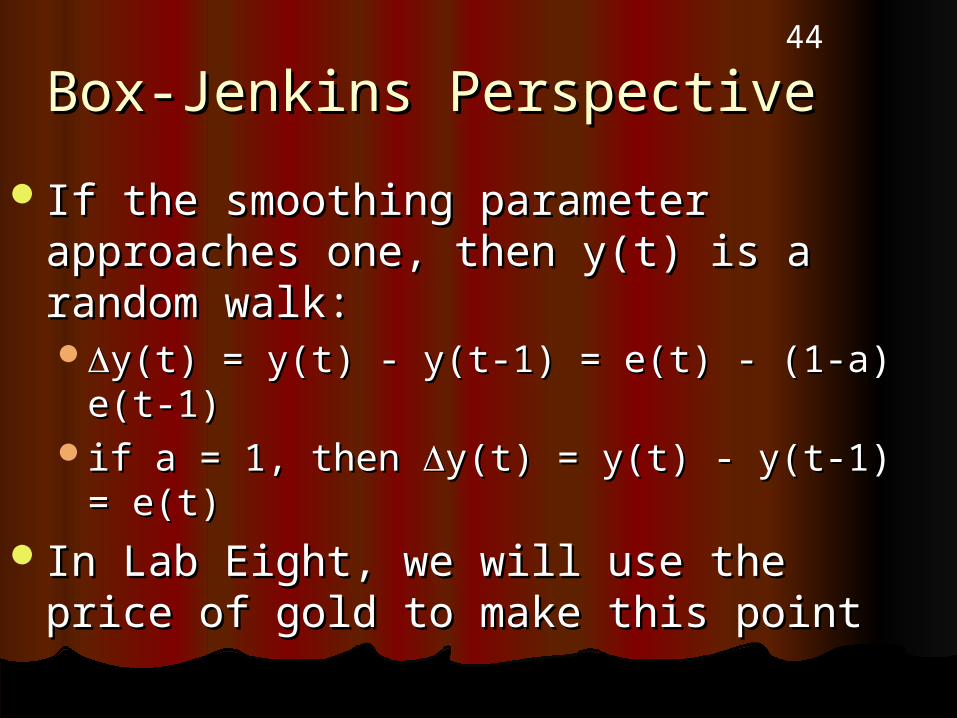
Box-Jenkins PerspectiveBox-Jenkins Perspective
If the smoothing parameter approaches If the smoothing parameter approaches one, then y(t) is a random walk:one, then y(t) is a random walk:y(t) = y(t) - y(t-1) = e(t) - (1-a) e(t-1)y(t) = y(t) - y(t-1) = e(t) - (1-a) e(t-1)if a = 1, then if a = 1, then y(t) = y(t) - y(t-1) = e(t) y(t) = y(t) - y(t-1) = e(t)
In Lab Eight, we will use the price of In Lab Eight, we will use the price of gold to make this pointgold to make this point

45
360
380
400
420
440
460
10 20 30 40 50 60 70
GOLD
Weekly Closing Price of Gold , Nov. 14, 2003-April 29, 2005

46

47

48

49Box-Jenkins PerspectiveBox-Jenkins PerspectiveThe levels or forecast, L(t), is a The levels or forecast, L(t), is a
geometric distributed lag of past geometric distributed lag of past observations of the series, y(t), hence observations of the series, y(t), hence the name “exponential” smoothingthe name “exponential” smoothingL(t) = a*y(t-1) + (1 - a)*L(t-1)L(t) = a*y(t-1) + (1 - a)*L(t-1)L(t) = a*y(t-1) + (1 - a)*ZL(t)L(t) = a*y(t-1) + (1 - a)*ZL(t)L(t) - (1 - a)*ZL(t) = a*y(t-1) L(t) - (1 - a)*ZL(t) = a*y(t-1) [1 - (1-a)Z] L(t) = a*y(t-1) [1 - (1-a)Z] L(t) = a*y(t-1) L(t) = {1/ [1 - (1-a)Z]} a*y(t-1) L(t) = {1/ [1 - (1-a)Z]} a*y(t-1) L(t) = [1 +(1-a)Z + (1-a)L(t) = [1 +(1-a)Z + (1-a)2 2 ZZ2 2 + …] a*y(t-1)+ …] a*y(t-1)L(t) = a*y(t-1) + (1-a)*a*y(t-2) + (1-L(t) = a*y(t-1) + (1-a)*a*y(t-2) + (1-
a)a)22a*y(t-3) + ….a*y(t-3) + ….

50
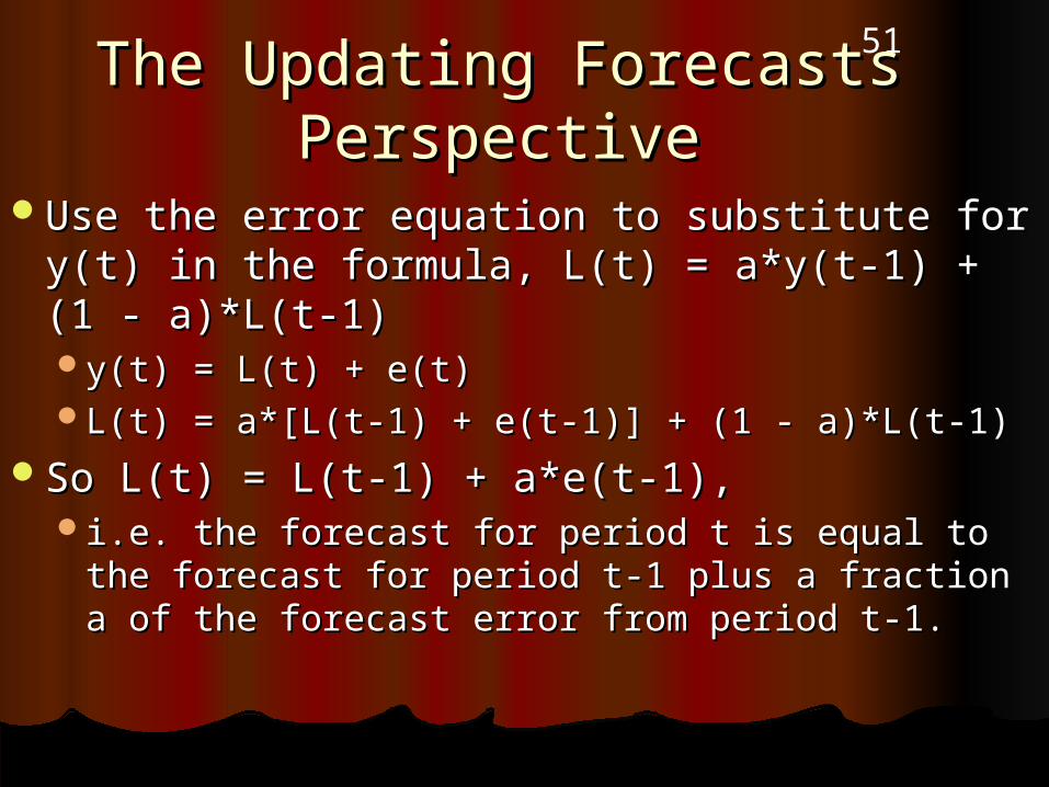
51The Updating Forecasts The Updating Forecasts PerspectivePerspective
Use the error equation to substitute for Use the error equation to substitute for y(t) in the formula, L(t) = a*y(t-1) + (1 - y(t) in the formula, L(t) = a*y(t-1) + (1 - a)*L(t-1)a)*L(t-1)y(t) = L(t) + e(t)y(t) = L(t) + e(t)L(t) = a*[L(t-1) + e(t-1)] + (1 - a)*L(t-1)L(t) = a*[L(t-1) + e(t-1)] + (1 - a)*L(t-1)
So L(t) = L(t-1) + a*e(t-1), So L(t) = L(t-1) + a*e(t-1), i.e. the forecast for period t is equal to the i.e. the forecast for period t is equal to the
forecast for period t-1 plus a fraction a of the forecast for period t-1 plus a fraction a of the forecast error from period t-1.forecast error from period t-1.

52Part III. Double Exponential Part III. Double Exponential
Smoothing Smoothing With double exponential smoothing, one With double exponential smoothing, one
estimates a “trend” term, R(t), as well estimates a “trend” term, R(t), as well as a levels term, L(t), so it is possible to as a levels term, L(t), so it is possible to forecast, f(t), out more than one periodforecast, f(t), out more than one period
f(t+k) = L(t) + k*R(t), k>=1f(t+k) = L(t) + k*R(t), k>=1L(t) = a*y(t) + (1-a)*[L(t-1) + R(t-1)]L(t) = a*y(t) + (1-a)*[L(t-1) + R(t-1)]R(t) = b*[L(t) - L(t-1)] + (1-b)*R(t-1)R(t) = b*[L(t) - L(t-1)] + (1-b)*R(t-1)
so the trend, R(t), is a geometric distributed so the trend, R(t), is a geometric distributed lag of the change in levels, lag of the change in levels, L(t)L(t)
1k 1k 1k
1k

53
If the smoothing parameters a = b, If the smoothing parameters a = b, then we have double exponential then we have double exponential smoothingsmoothing
If the smoothing parameters are If the smoothing parameters are different, then it is the simplest different, then it is the simplest version of Holt-Winters smoothingversion of Holt-Winters smoothing
Part III. Double Exponential Part III. Double Exponential SmoothingSmoothing
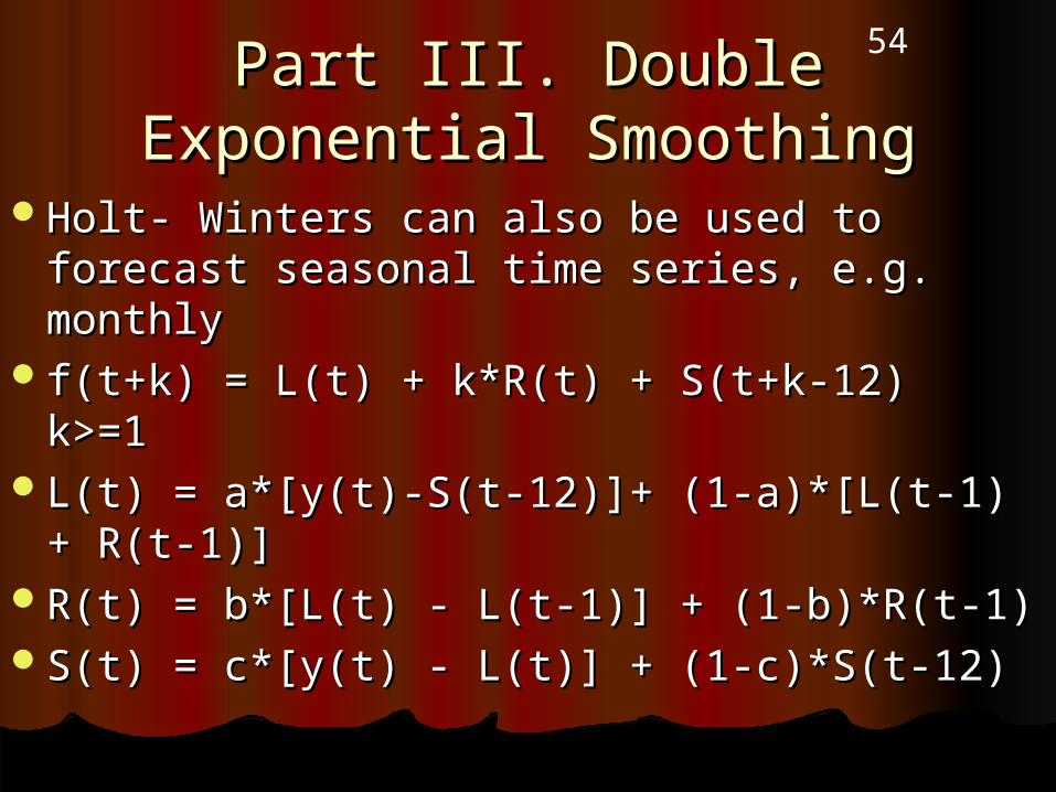
54Part III. Double Exponential Part III. Double Exponential SmoothingSmoothing
Holt- Winters can also be used to forecast Holt- Winters can also be used to forecast seasonal time series, e.g. monthlyseasonal time series, e.g. monthly
f(t+k) = L(t) + k*R(t) + S(t+k-12) k>=1f(t+k) = L(t) + k*R(t) + S(t+k-12) k>=1L(t) = a*[y(t)-S(t-12)]+ (1-a)*[L(t-1) + R(t-L(t) = a*[y(t)-S(t-12)]+ (1-a)*[L(t-1) + R(t-
1)]1)]R(t) = b*[L(t) - L(t-1)] + (1-b)*R(t-1)R(t) = b*[L(t) - L(t-1)] + (1-b)*R(t-1)S(t) = c*[y(t) - L(t)] + (1-c)*S(t-12)S(t) = c*[y(t) - L(t)] + (1-c)*S(t-12)

55
Part V. Intervention AnalysisPart V. Intervention Analysis

56
Intervention AnalysisIntervention Analysis
The approach to intervention The approach to intervention analysis parallels Box-Jenkins in that analysis parallels Box-Jenkins in that the actual estimation is conducted the actual estimation is conducted after pre-whitening, to the extent after pre-whitening, to the extent that non-stationarity such as trend that non-stationarity such as trend and seasonality are removedand seasonality are removed
Example: preview of Lab 8Example: preview of Lab 8

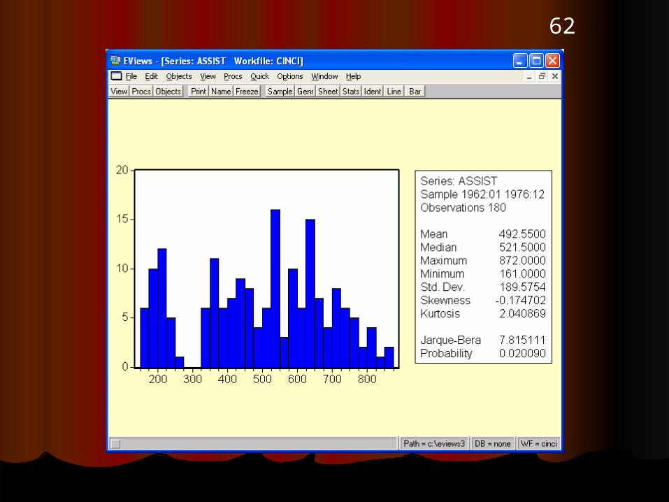
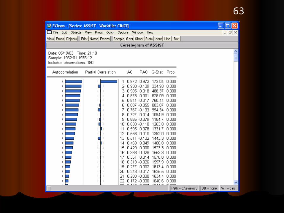
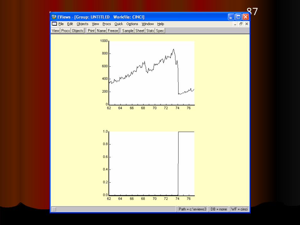
57Telephone Directory Telephone Directory AssistanceAssistance
A telephone company was receiving A telephone company was receiving increased demand for free directory increased demand for free directory assistance, i.e. subscribers asking assistance, i.e. subscribers asking operators to look up numbers. This operators to look up numbers. This was increasing costs and the was increasing costs and the company changed policy, providing a company changed policy, providing a number of free assisted calls to number of free assisted calls to subscribers per month, but charging subscribers per month, but charging a price per call after that number. a price per call after that number.

58Telephone Directory Telephone Directory AssistanceAssistance
This policy change occurred at a This policy change occurred at a known time, March 1974known time, March 1974
The time series is for calls with The time series is for calls with directory assistance per monthdirectory assistance per month
Did the policy change make a Did the policy change make a difference?difference?

59

60
The simple-minded approachThe simple-minded approach
=549 - 162
=387

61
62
63
64
PrinciplePrinciple
The event may cause a change, and The event may cause a change, and affect time series characteristicsaffect time series characteristics
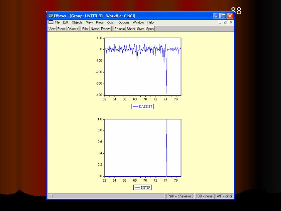
Consequently, consider the pre-event Consequently, consider the pre-event period, January 1962 through period, January 1962 through February 1974, the event March February 1974, the event March 1974, and the post-event period, 1974, and the post-event period, April 1974 through December 1976April 1974 through December 1976
First difference and then seasonally First difference and then seasonally difference the entire seriesdifference the entire series
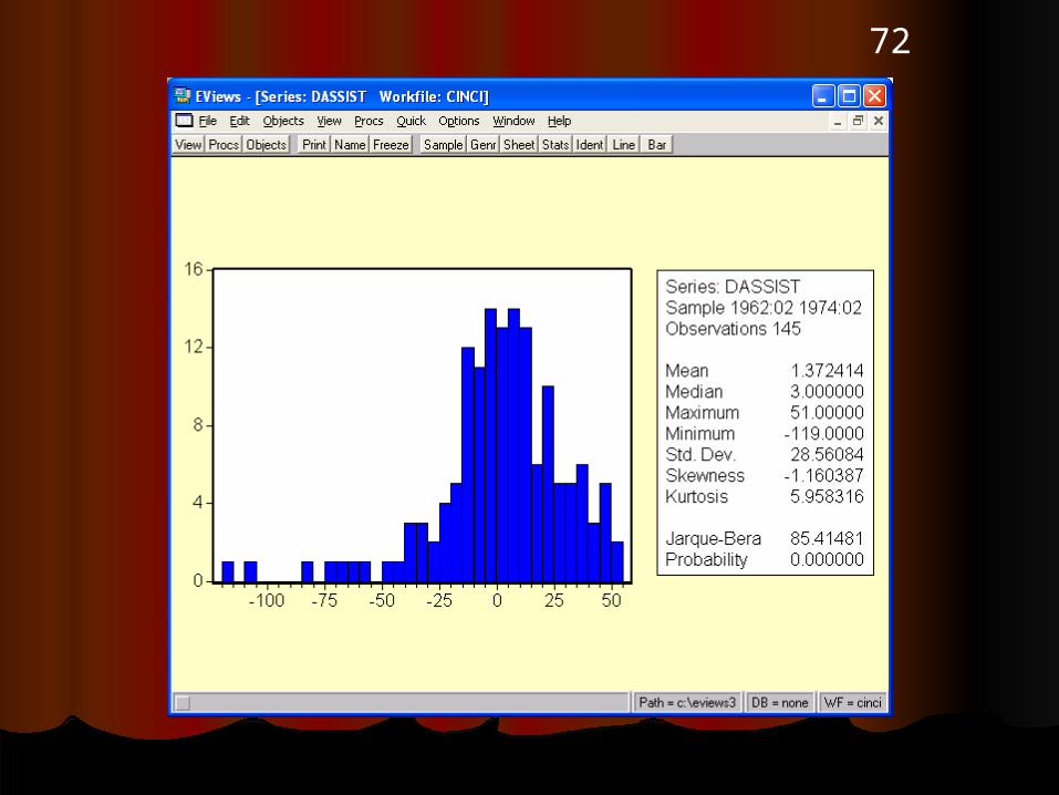
65Analysis: Entire Differenced Analysis: Entire Differenced SeriesSeries

66

67

68

69

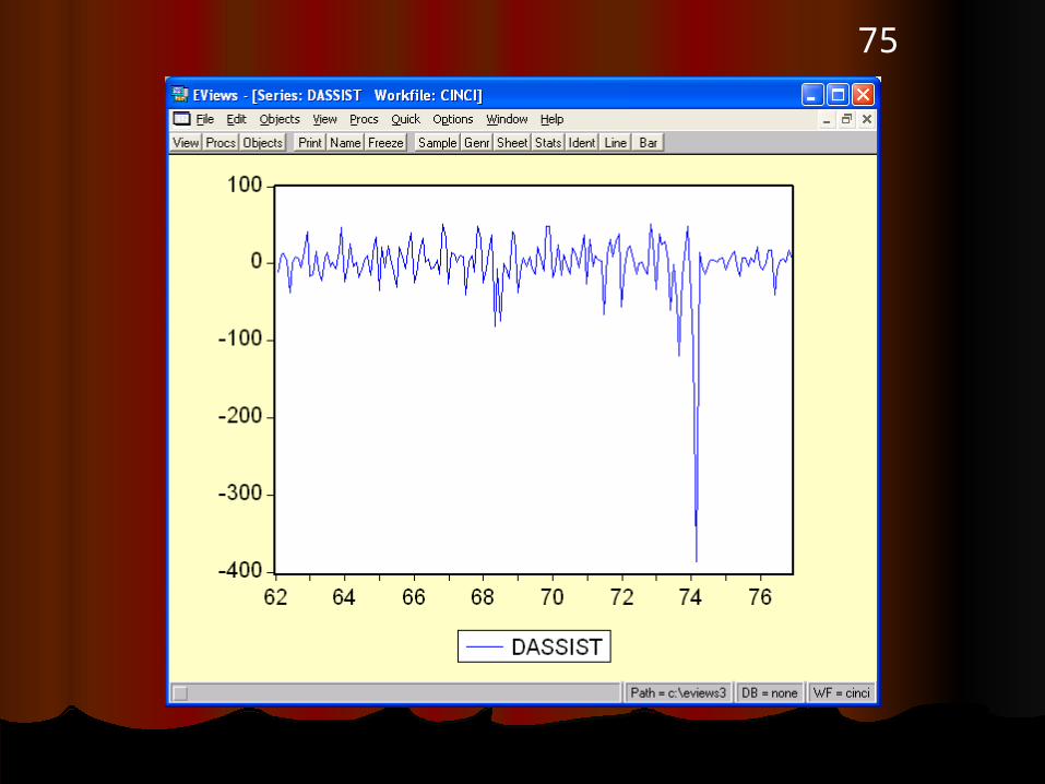
70Analysis: Pre-Event Analysis: Pre-Event DifferencesDifferences

71
72
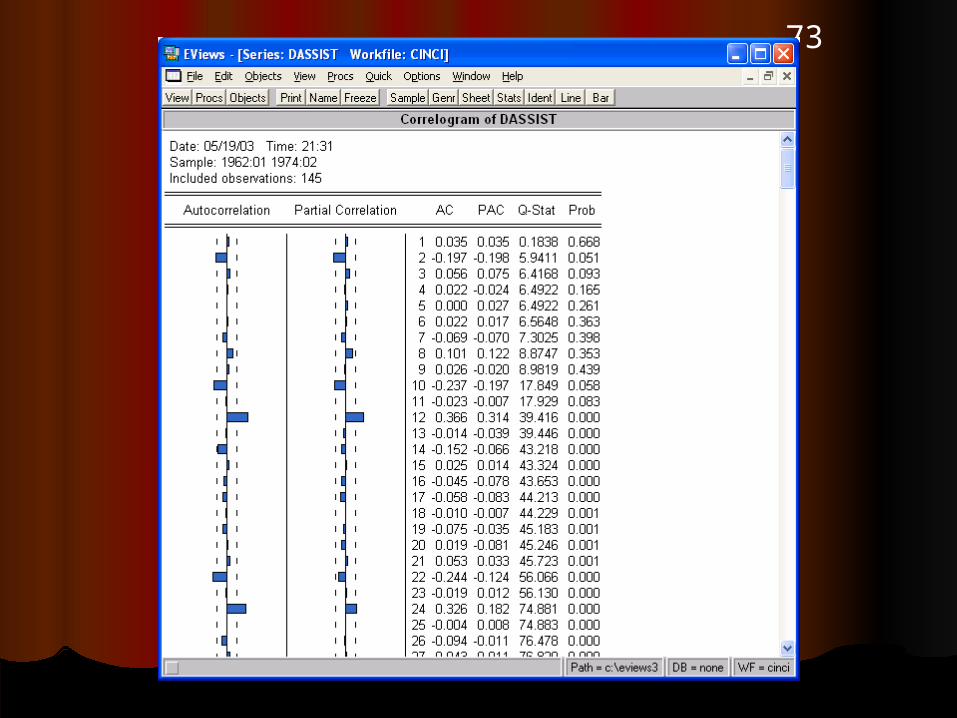
73
74
So Seasonal NonstationaritySo Seasonal Nonstationarity
It was masked in the entire sample It was masked in the entire sample by the variance caused by the by the variance caused by the difference from the eventdifference from the event
The seasonality was revealed in the The seasonality was revealed in the pre-event differenced series pre-event differenced series
75

76
Pre-Event AnalysisPre-Event Analysis
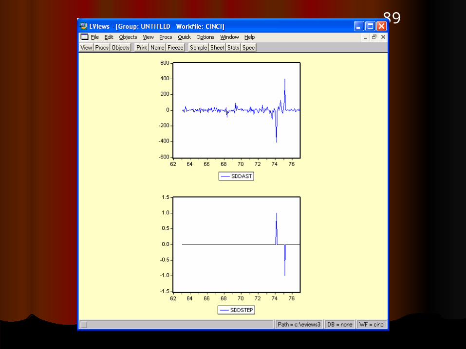
Seasonally differenced, differenced Seasonally differenced, differenced series series

77

78

79
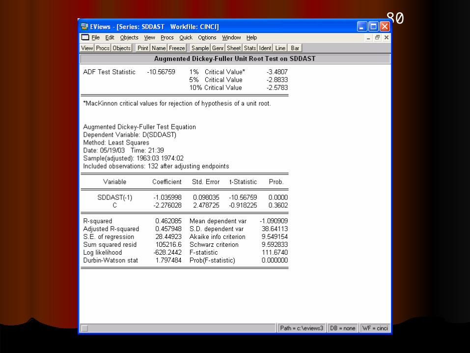
80

81
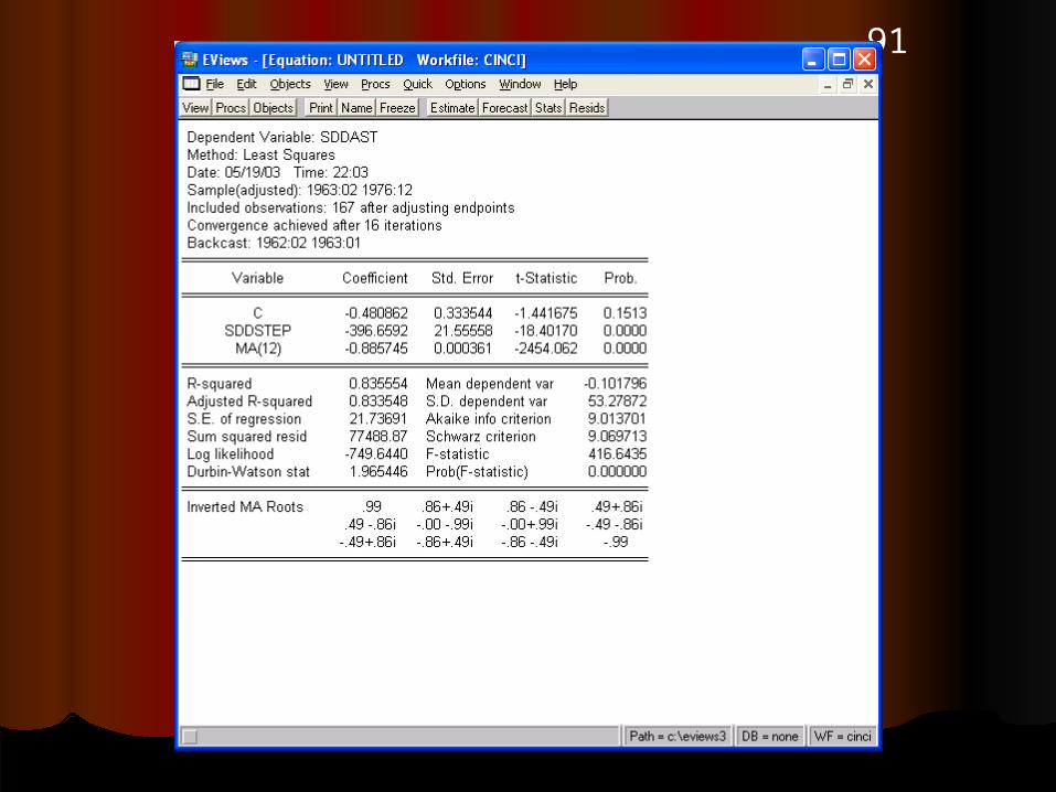
Pre-Event Box-Jenkins ModelPre-Event Box-Jenkins Model
[1-Z[1-Z12 12 ][1 –Z]Assist(t) = WN(t) – a*WN(t-][1 –Z]Assist(t) = WN(t) – a*WN(t-12)12)

82

83

84

85
Modeling the EventModeling the Event
Step functionStep function

86
Entire SeriesEntire Series
Assist and StepAssist and StepDassist and DstepDassist and DstepSddast sddstepSddast sddstep
87
88
89

90
Model of Series and EventModel of Series and Event
Pre-Event Model: [1-ZPre-Event Model: [1-Z12 12 ][1 –Z]Assist(t) = ][1 –Z]Assist(t) = WN(t) – a*WN(t-12)WN(t) – a*WN(t-12)
In Levels Plus Event: Assist(t)=[WN(t) – In Levels Plus Event: Assist(t)=[WN(t) – a*WN(t-12)]/[1-Z]*[1-Za*WN(t-12)]/[1-Z]*[1-Z1212] + (-b)*step] + (-b)*step
Estimate: [1-ZEstimate: [1-Z12 12 ][1 –Z]Assist(t) = WN(t) ][1 –Z]Assist(t) = WN(t) – a*WN(t-12) + (-b)* [1-Z– a*WN(t-12) + (-b)* [1-Z12 12 ][1 –Z]*step][1 –Z]*step
91

92
93
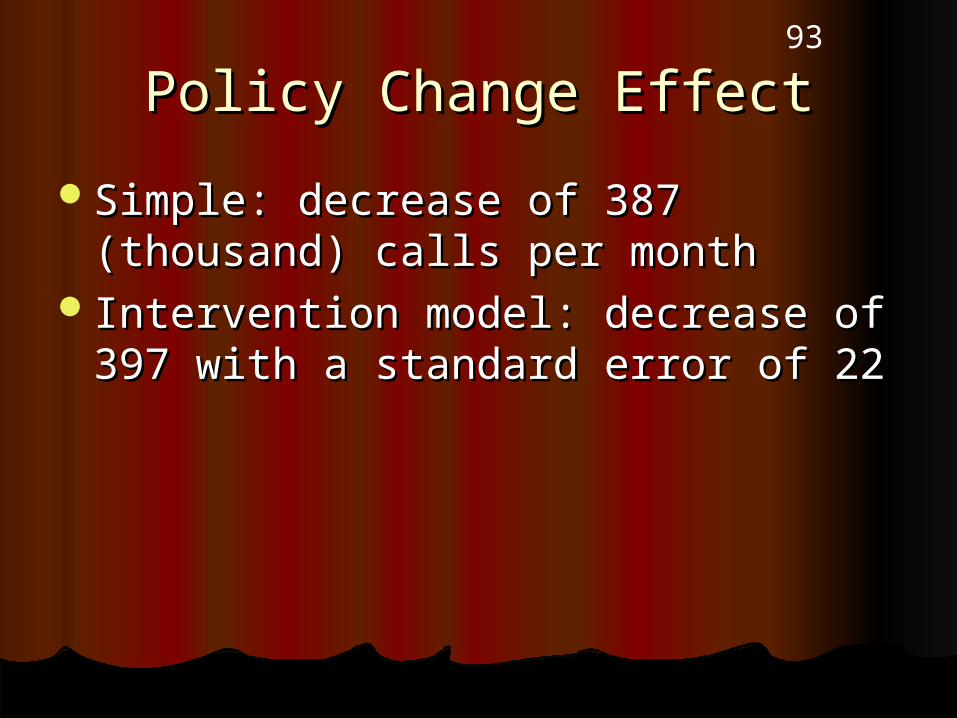
Policy Change EffectPolicy Change Effect
Simple: decrease of 387 (thousand) Simple: decrease of 387 (thousand) calls per monthcalls per month
Intervention model: decrease of 397 Intervention model: decrease of 397 with a standard error of 22with a standard error of 22

94
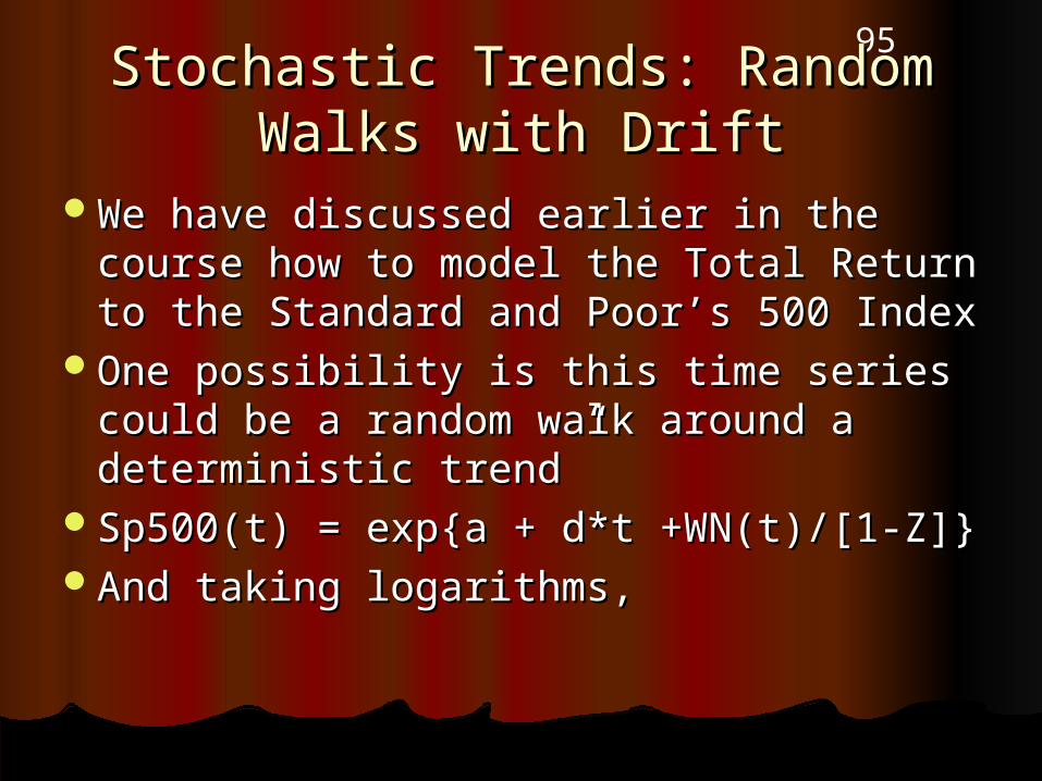
95Stochastic Trends: Random Stochastic Trends: Random
Walks with DriftWalks with DriftWe have discussed earlier in the We have discussed earlier in the
course how to model the Total Return course how to model the Total Return to the Standard and Poor’s 500 Indexto the Standard and Poor’s 500 Index
One possibility is this time series could One possibility is this time series could be a random walk around a be a random walk around a deterministic trend”deterministic trend”
Sp500(t) = exp{a + d*t +WN(t)/[1-Z]}Sp500(t) = exp{a + d*t +WN(t)/[1-Z]}And taking logarithms,And taking logarithms,

96Stochastic Trends: Random Stochastic Trends: Random
Walks with DriftWalks with Drift Lnsp500(t) = a + d*t + WN(t)/[1-Z]Lnsp500(t) = a + d*t + WN(t)/[1-Z] Lnsp500(t) –a –d*t = WN(t)/[1-Z]Lnsp500(t) –a –d*t = WN(t)/[1-Z] Multiplying through by the difference Multiplying through by the difference
operator, operator, = [1-Z]= [1-Z] [1-Z][Lnsp500(t) –a –d*t] = WN(t-1)[1-Z][Lnsp500(t) –a –d*t] = WN(t-1)
[LnSp500(t) – a –d*t] - [LnSp500(t-1) – a –[LnSp500(t) – a –d*t] - [LnSp500(t-1) – a –d*(t-1)] = WN(t)d*(t-1)] = WN(t)
Lnsp500(t) = d + WN(t)Lnsp500(t) = d + WN(t)

97
So the fractional change in the total return So the fractional change in the total return to the S&P 500 is drift, d, plus white noiseto the S&P 500 is drift, d, plus white noise
More generally, More generally, y(t) = a + d*t + {1/[1-Z]}*WN(t)y(t) = a + d*t + {1/[1-Z]}*WN(t)[y(t) –a –d*t] = {1/[1-Z]}*WN(t)[y(t) –a –d*t] = {1/[1-Z]}*WN(t)[y(t) –a –d*t]- [y(t-1) –a –d*(t-1)] = WN(t)[y(t) –a –d*t]- [y(t-1) –a –d*(t-1)] = WN(t)[y(t) –a –d*t]= [y(t-1) –a –d*(t-1)] + WN(t)[y(t) –a –d*t]= [y(t-1) –a –d*(t-1)] + WN(t)Versus the possibility of an ARONE:Versus the possibility of an ARONE:
98
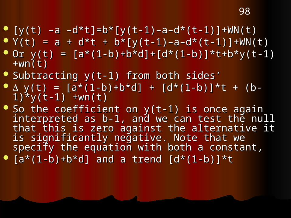
[y(t) –a –d*t]=b*[y(t-1)–a–d*(t-1)]+WN(t)[y(t) –a –d*t]=b*[y(t-1)–a–d*(t-1)]+WN(t) Y(t) = a + d*t + b*[y(t-1)–a–d*(t-1)]+WN(t)Y(t) = a + d*t + b*[y(t-1)–a–d*(t-1)]+WN(t) Or y(t) = [a*(1-b)+b*d]+[d*(1-b)]*t+b*y(t-1) Or y(t) = [a*(1-b)+b*d]+[d*(1-b)]*t+b*y(t-1)
+wn(t)+wn(t) Subtracting y(t-1) from both sides’Subtracting y(t-1) from both sides’ y(t) = [a*(1-b)+b*d] + [d*(1-b)]*t + (b-1)*y(t-1) y(t) = [a*(1-b)+b*d] + [d*(1-b)]*t + (b-1)*y(t-1)
+wn(t)+wn(t) So the coefficient on y(t-1) is once again So the coefficient on y(t-1) is once again
interpreted as b-1, and we can test the null that interpreted as b-1, and we can test the null that this is zero against the alternative it is this is zero against the alternative it is significantly negative. Note that we specify the significantly negative. Note that we specify the equation with both a constant, equation with both a constant,
[a*(1-b)+b*d] and a trend [d*(1-b)]*t [a*(1-b)+b*d] and a trend [d*(1-b)]*t

99Part IV. Dickey Fuller Tests: Part IV. Dickey Fuller Tests: TrendTrend

100
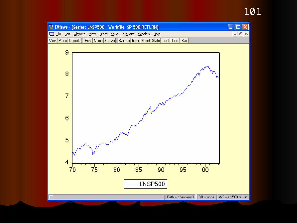
ExampleExample
Lnsp500(t) from Lab 2Lnsp500(t) from Lab 2
101
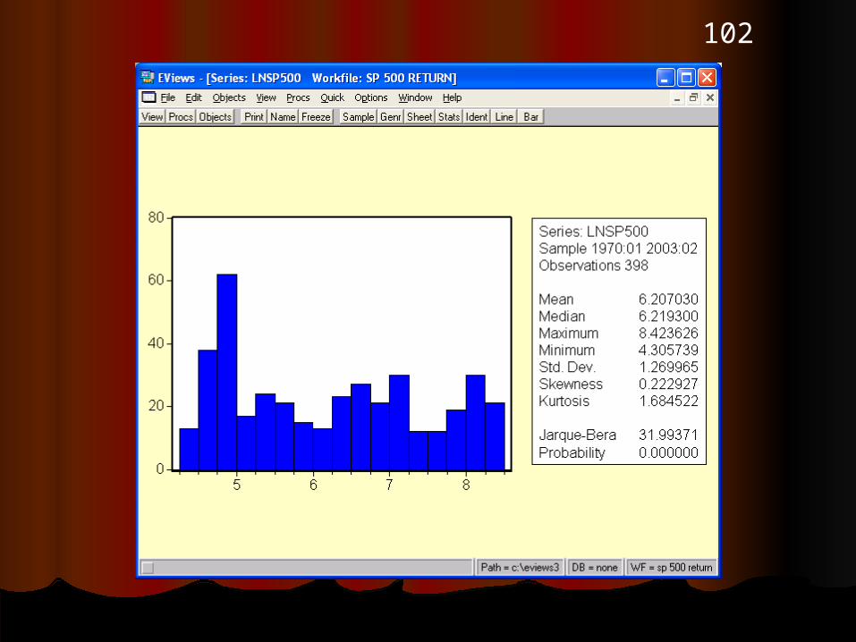
102
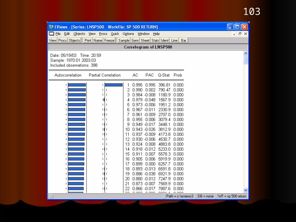
103

104
Related Documents