Parametric Formulation of the Finite-Volume Theory for Functionally Graded Materials---Part II: Numerical Results

1

walegosptawMa

ottal�tesescsm

Jr

J

Downlo

Marcio A. A. Cavalcante

Severino P. C. Marques

Center of Technology,Federal University of Alagoas,

Maceio, Alagoas, Brazil

Marek-Jerzy PinderaCivil Engineering Department,

University of Virginia,Charlottesville, VA 22903

Parametric Formulation of theFinite-Volume Theory forFunctionally GradedMaterials—Part I: AnalysisThe recently reconstructed higher-order theory for functionally graded materials is fur-ther enhanced by incorporating arbitrary quadrilateral subcell analysis capabilitythrough a parametric formulation. This capability significantly improves the efficiency ofmodeling continuous inclusions with arbitrarily-shaped cross sections of a graded mate-rial’s microstructure previously approximated using discretization based on rectangularsubcells, as well as modeling of structural components with curved boundaries. Part I ofthis paper describes the development of the local conductivity and stiffness matrices fora quadrilateral subcell which are then assembled into global matrices in an efficientmanner following the finite-element assembly procedure. Part II verifies the parametricformulation through comparison with analytical solutions for homogeneous curved struc-tural components and graded components where grading is modeled using piecewiseuniform thermoelastic moduli assigned to each discretized region. Results for a hetero-geneous microstructure in the form of a single inclusion embedded in a matrix phase arealso generated and compared with the exact analytical solution, as well as with theresults obtained using the original reconstructed theory based on rectangular discretiza-tion and finite-element analysis. �DOI: 10.1115/1.2722312�

Keywords: functionally graded materials, finite-volume theory, parametric formulation

IntroductionFunctionally graded materials �FGMs� are multiphase materials

ith engineered microstructures which produce property gradientsimed at optimizing structural response under different types ofoads �thermal, mechanical, electrical, optical, etc.�. These prop-rty gradients are produced in several ways, for example byradual variation of the content of one phase �ceramic� relative tother �metallic� used in thermal barrier coatings, or by using aufficiently large number of constituent phases with differentroperties. Developed by Japanese researchers in the mid-1980s,hese materials continue to evolve and to find new applications inreas other than the thermal protection/management structures forhich they had been originally developed, cf. Suresh andortensen �1�, Miyamoto et al. �2�, Paulino �3�, Chatzigeorgiou

nd Charalambakis �4�.The use of graded material concepts in structural design and

ptimization requires the development of appropriate analysisechniques which account for the spatially variable microstruc-ures in this class of materials. Presently, there are two approachesvailable to analyze the response of FGMs to thermomechanicaloads, called coupled and uncoupled approaches, Pindera et al.5�. In the uncoupled approach, the graded material’s microstruc-ure is replaced by equivalent homogenized properties which areither determined from micromechanics considerations or as-umed a priori. This results in a boundary-value problem withither continuously or discretely variable elastic moduli at thecale at which the analysis is conducted, called macroscale. In theoupled approach originally proposed by Aboudi et al. �6�, andummarized in a review paper by Aboudi et al. �7�, the material’sicrostructure is explicitly taken into account by performing the

Contributed by the Applied Mechanics Division of ASME for publication in theOURNAL OF APPLIED MECHANICS. Manuscript received June 6, 2006; final manuscript

ournal of Applied Mechanics Copyright © 20

aded 14 Sep 2007 to 128.143.34.99. Redistribution subject to ASME

analysis at the microscale. In particular, in the original formula-tion of this so-called higher-order theory, a two-step discretizationinvolving generic cells and subcells is employed to capture thegraded material’s heterogeneous microstructure. Subsequently,thermal and displacement fields within each subcell are approxi-mated using quadratic expansions in local coordinates, and theunknown coefficients associated with the different-order terms areobtained by satisfying various moments of the field equations in avolume-averaged sense in each subcell, followed by the applica-tion of continuity conditions within each generic cell, and betweenadjacent cells, in a surface-average sense together with the im-posed boundary conditions. We mention that surface averaging ofcontinuity conditions was proposed by Achenbach �8� in the con-text of the author’s cell model for unidirectional composites.

This approach has recently been reconstructed by Bansal andPindera �9� and Zhong et al. �10� based on a simplified volumediscretization using subcells as the fundamental subvolumes, inplace of the two-level discretization employed in the original con-struction. The use of subcells as the fundamental subvolumes, inturn, facilitated the implementation of the local/global stiffnessmatrix formulation, Bufler �11�, Pindera �12�, into the solutionprocedure for the unknown subcell surface-averaged interfacialdisplacements which became the primary unknown quantities inthe reconstructed theory. The reconstruction has also revealed thatthe model’s theoretical framework is based on direct satisfactionof the field equations within each subcell, in contrast to the origi-nal construction wherein higher-order moments of the equilibriumequations were also satisfied, thereby erroneously suggesting thismodel to be a version of a micropolar continuum theory. Thesignificantly simplified theoretical structure of this so-calledhigher-order theory in conjunction with the implementation of thelocal/global stiffness matrix approach also resulted in a substantialreduction in the final system of equations for the unknown quan-tities, thereby making it possible to analyze realistic graded mi-

SEPTEMBER 2007, Vol. 74 / 93507 by ASME

license or copyright, see http://www.asme.org/terms/Terms_Use.cfm

wcafiero

rtmsefmtppi

2M

tweTstpu�l

Tsc

¯

F„

x

9

Downlo

ith the theory’s original formulation. Equally important, the re-onstruction has revealed the method to be a finite-volume directveraging technique with clearly discernible similarities and dif-erences between the finite-volume technique used in fluid dynam-cs problems, cf. Versteeg and Malalasekera �13�, and the finite-lement method, as reported by Pindera et al. �14�. Thiseconstruction made it possible to further develop the method inrder to increase its efficiency and applicability.

In this communication, we continue the development of theeconstructed Cartesian-version of the theory, herein referred to ashe standard finite-volume theory, by incorporating parametric

apping capability in order to enable efficient modeling of micro-tructures that cannot be easily modeled using rectangular subcellsmployed in the standard theory. The parametric formulation of-ers the same flexibility as the finite-element method for modelingicrostructures and geometries with curved and rectilinear fea-

ures, while retaining its quick convergence characteristics in theresence of highly heterogeneous microstructures. We begin byroviding a brief outline of the reconstructed finite-volume theoryn order to set the stage for the parametric formulation.

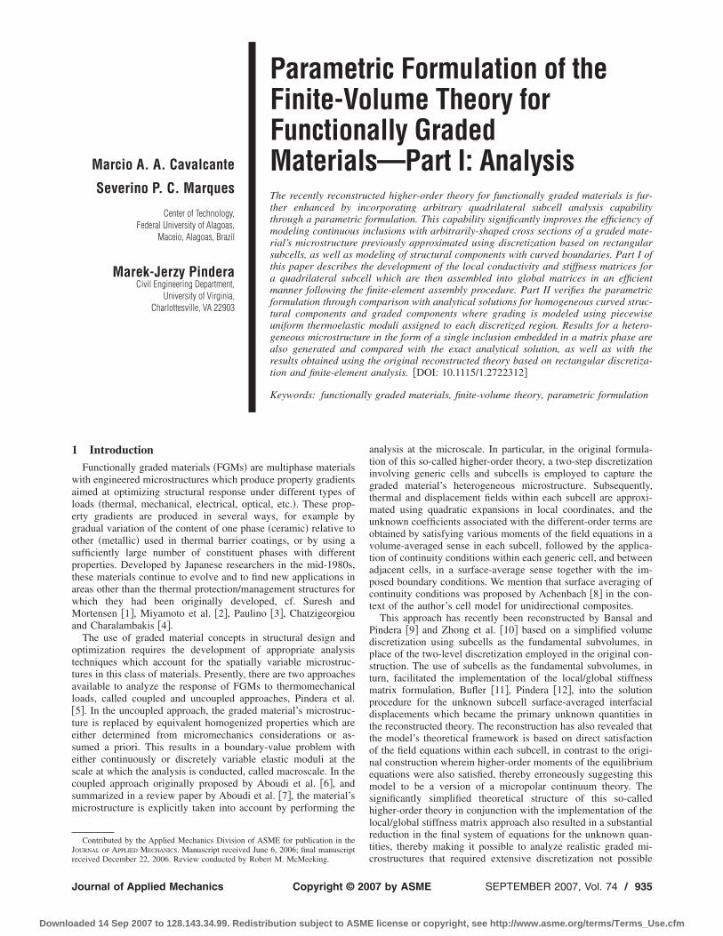
The Finite-Volume Theory for Functionally GradedaterialsIn the standard version of the finite-volume theory for FGMs,

he material microstructure is discretized into N� columns, each ofidth h�, spanning the distance H along the x2-axis, and N� rows,

ach of height l�, spanning the distance L along the x3-axis, Fig. 1.his results in a grid of N��N� �� ,�� subcells of h�� l� dimen-ions, which is used to approximate the heterogeneous microstruc-ure by assigning appropriate moduli to each subcell. The tem-erature and displacement fields are approximated in each subcellsing quadratic expansions in the local subcell coordinatesx2

��� , x3���� attached to the subcell’s center. For the thermal prob-

em we have

T��,�� = T�00���,�� + x2

���T�10���,�� + x3

���T�01���,�� +

1

2�3x2

���2 −h�

2

4�T�20�

��,��

+1

2�3x3

���2 −l�2

4�T�02�

��,�� �1�

he heat flux components qi��,�� at any point passing through a

ubcell �� ,�� are then obtained from the Fourier’s law of heat

ig. 1 Simplified discretization of a graded microstructureleft… into rectangular subcells with the local coordinate system

2„�…−x3

„�…„right… used in the reconstructed finite-volume theory

onduction

36 / Vol. 74, SEPTEMBER 2007

aded 14 Sep 2007 to 128.143.34.99. Redistribution subject to ASME

qi��,�� = − ki

��,���T��,��

�xi�·� �i = 2,3; no sum� �2�

where ki��,�� are the heat conductivity coefficients of the material

in the subcell �� ,��. For the mechanical problem

ui��,�� = Wi�00�

��,�� + x2���Wi�10�

��,�� + x3���Wi�01�

��,�� +1

2�3x2

���2 −h�

2

4�Wi�20�

��,��

+1

2�3x3

���2 −l�2

4�Wi�02�

��,�� �3�

where i=2,3 for plane problems. The stress components at anypoint within the �� ,�� subcell are obtained, upon the use of strain-displacement equations, from the generalized Hooke’s law

�ij��,�� = Cijkl

��,���kl��,�� − �ij

th��,�� �4�

where �ijth��,��=Cijkl

��,���kl��,��

�T=�ij��,��

�T.Subsequently, conductivity and stiffness matrices are con-

structed for each subcell by relating the surface-averaged tempera-

ture and displacement vectors, T��,�� and u��,��, to the correspond-

ing surface-averaged heat flux and traction vectors, Q��,�� andt��,��, whose components are

T��,�� = �T2+,T2−,T3+,T3−���,��T

Q��,�� = �Q22+,Q2

2−,Q33+,Q3

3−���,��T

u��,�� = �u22+, u3

2+, u22−, u3

2−, u23+, u3

3+, u23−, u3

3−���,��T

t��,�� = �t22+, t3

2+, t22−, t3

2−, t23+, t3

3+, t23−, t3

3−���,��T �5�

where the superscripts 2, 3 identify the direction of the unit nor-mal to the given face relative to the fixed subcell coordinates�x2

��� , x3����, and denote the actual sense. The subscripts 2, 3

denote a vectorial quantity’s component. Traction components areexpressed in terms of stress components associated with a particu-lar subcell face through Cauchy’s relations

tin��,��

= � ji��,��nj

��,�� �6�

and n��,�� is the unit normal to a given face of the �� ,�� subcell.Finally, the surface averages are defined in the standard way, asfor example

T2±��,�� =1

l��

−l�/2

l�/2

T��,���±h�

2, x3

����dx3���

T3±��,�� =1

h��

−h�/2

h�/2

T��,���x2���, ±

l�

2�dx2

��� �7�

for the surface-averaged temperatures, with similar expressionsfor the remaining field variables.

For the thermal problem, there are five coefficients which mustbe related to the four surface-averaged temperatures. Four rela-tions are provided by the definitions of the surface-averaged tem-peratures. Satisfaction of the heat conduction equation in the large

�S��,��

qi��,��ni

��,��dS = 0 �8�

provides the additional relation required in the local conductivitymatrix construction carried out by averaging the heat flux equa-tions along each of the four faces, which yields

Q��,�� = ���,��T��,�� �9�For the mechanical problem, there are ten coefficients which

must be related to the eight surface-averaged displacement com-

Transactions of the ASME

license or copyright, see http://www.asme.org/terms/Terms_Use.cfm

set

Eot

easaaaetcu

ut

k

a

s

Tairdaomma

wsti

3T

sgdF

J

Downlo

urface-averaged displacement components. The additional twoquations are obtained by satisfying the stress equilibrium equa-ions in each subcell in the large

�S��,��

tin��,��

dS = 0, i = 2,3 �10�

valuating the surface-averaged traction components on each facef the �� ,�� subcell leads to the local stiffness matrix relation ofhe form

t��,�� = K��,��u��,�� + ���,��T��,�� �11�Assembly of the local conductivity and stiffness matrices by

nforcing the continuity of both surface-averaged temperaturesnd displacements, and heat fluxes and tractions, together with thepecified boundary conditions, determines the unknown surface-veraged temperatures and displacements from which local fieldsre obtained through constitutive and gradient relations. In thispproach, the redundant temperature and displacement continuityquations are eliminated by setting the surface-averaged tempera-ures and displacements at the interfaces associated with the adja-ent subcells �� ,��, ��+1,��, and �� ,��, �� ,�+1� to commonnknowns,

T2+��,�� = T2−��+1,�� = T2��+1,�� T3+��,�� = T3−��,�+1� = T3��,�+1�

ui2+��,�� = ui

2−��+1,�� = ui2��+1,�� ui

3+��,�� = ui3−��,�+1� = ui

3��,�+1�

i = 2,3 �12�pon application of the heat flux and traction continuity condi-ions at these common interfaces

Q2+��,�� − Q2

−��+1,�� = 0 Q3+��,�� − Q3

−��,�+1� = 0

ti2+��,�� + ti

2−��+1,�� = 0 ti3+��,�� + ti

3−��,�+1� = 0 i = 2,3

�13�The resulting global thermal conductivity matrix relates the un-

nown interfacial surface-averaged temperatures �including those

t the external boundaries� represented by T to the corresponding

urface-averaged heat fluxes represented by Q

�T = Q �14�

he vector Q consists mainly of zeros which are obtained afterpplying interfacial heat flux continuity conditions across eachnterface separating adjacent subcells, with the nonzero terms rep-esenting surface-averaged heat fluxes along each portion of theiscretized boundary. The above system of equations is modifiedccordingly when the boundary conditions are specified in termsf applied temperatures. Similarly, the resulting global stiffnessatrix relates the unknown interfacial surface-averaged displace-ents �including those at the external boundaries� to the surface-

veraged tractions prescribed at the external boundaries

KU = t + �T �15�ith the known surface-averaged temperatures obtained from the

olution of the thermal problem. The above system of equations ishen reduced to eliminate rigid body motion, and modified accord-ng to the specified boundary conditions.

Parametric Formulation of the Finite-VolumeheoryThe parametric formulation enables the use of quadrilateral

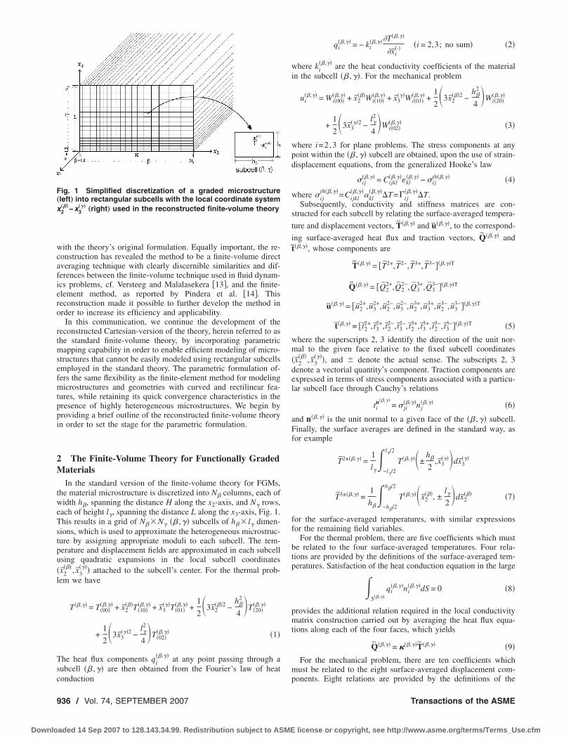
ubcells in approximating the heterogeneous microstructure of araded material, thereby making the modeling of microstructuraletails with curvilinear boundaries more efficient, as illustrated in

ournal of Applied Mechanics

aded 14 Sep 2007 to 128.143.34.99. Redistribution subject to ASME

rectangular and quadrilateral subcells. It is based on a mapping ofa reference square subcell in the -� plane onto a subcell in thex-y plane of the actual microstructure. The mapping facilitates thedevelopment of local conductivity and stiffness matrices for aquadrilateral subcell situated in the actual microstructure that re-late surface-averaged temperatures and displacements to the cor-responding heat fluxes and tractions acting on arbitrarily orientedrectlinear surfaces.

The important distinction between the parametric formulationand the version based on rectangular subcells described in Sec. 2is the absence of a local coordinate system associated with eachsubcell in the actual microstructure. Rather, global coordinates areemployed to describe the locations of quadrilateral subcell verti-ces in the actual microstructure, and thus the subcell’s placement.Global reference indexes are also assigned to the four faces ofeach subcell in the actual microstructure which are employed inthe construction of the connectivity matrix used to apply interfa-cial continuity and balance conditions in the assembly of the glo-bal conductivity and stiffness matrices. These indexes define thelocation of the local conductivity and stiffness matrix elements in

Fig. 2 Discretization of a square region containing a circularinclusion: „a… discretization based on 900 rectangular subcells;„b… discretization based on 500 quadrilateral subcells

the global systems of equations. We begin by describing the co-

SEPTEMBER 2007, Vol. 74 / 937

license or copyright, see http://www.asme.org/terms/Terms_Use.cfm

oom

iscdtcn�ng

w

cm

w

ase

Ffibcavsr

Fqm

9

Downlo

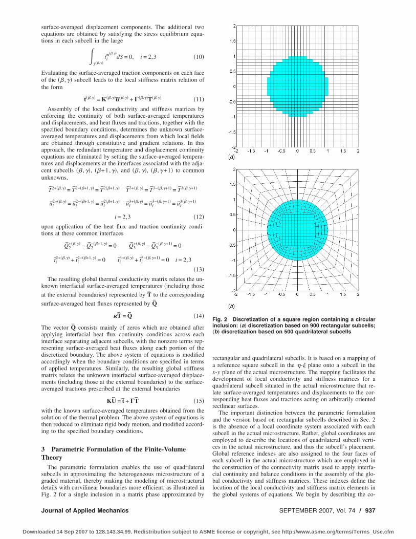
rdinate transformations associated with the mapping, and thenutline transient and mechanical analyses based on this parametricapping technique in the following sections.In the parametric formulation, the reference subcell is a square

n the -� plane bounded by −1��� +1 and −1�� +1. Ashown in Fig. 3, the vertices �−1,−1� of the reference subcellorrespond to the vertices �x1 ,y1� of the jth subcell in the actualiscretized microstructure. The vertices are numbered such thathe first set �x1 ,y1� is at the lower left corner and the numberingonvention increases in a counterclockwise fashion. The faces areumbered similarly such that the face Fi lies between the verticesxi ,yi� and �xi+1 ,yi+1� with i+1→1 when i=4. Thus the compo-ents of the unit normal vector n�i�= �nx

�i� ,ny�i�� to the face Fi are

iven by

nx�i� =

yi+1 − yi

Liny

�i� =xi − xi+1

Li

here

Li = ��xi+1 − xi�2 + �yi+1 − yi�2 �16�

The mapping of the point � ,�� in the reference subcell to theorresponding point �x ,y� in the subcell of the actual discretizedicrostructure is given by, Cavalcante �15�,

x�,�� = N1�,��x1 + N2�,��x2 + N3�,��x3 + N4�,��x4

y�,�� = N1�,��y1 + N2�,��y2 + N3�,��y3 + N4�,��y4

�17�here

N1�,�� =1

4�1 − ��1 − �� N2�,�� =

1

4�1 + ��1 − ��

N3�,�� =1

4�1 + ��1 + �� N4�,�� =

1

4�1 − ��1 + �� �18�

In both the thermal and mechanical problems, the field vari-bles are approximated by the same functional form based on aecond-order representation in the local coordinates of the refer-nce subcell in the -� plane, given by

f�,�� = F�00� + F�10� + �F�01� +1

2�32 − 1�F�20� +

1

2�3�2 − 1�F�02�

�19�

or the thermal problem, f� ,�� represents the local temperatureeld, whereas in the mechanical problem the above expressionecomes a vector function representing the two displacementomponents in the -� plane with two sets of coefficients associ-ted with each term in the expansion. Further, both sets of fieldariables are governed by similar differential equations and con-titutive equations relating flux-like quantities to the partial de-

ig. 3 Mapping of the reference subcell in the �-� plane onto auadrilateral subcell in the x-y plane of the actualicrostructure.

ivatives of the field variables. Therefore, in this section we de-

38 / Vol. 74, SEPTEMBER 2007

aded 14 Sep 2007 to 128.143.34.99. Redistribution subject to ASME

velop unifying relations containing common transformationmatrices between surface-averaged quantities in the two planes inorder to avoid duplication in the subsequent sections dealing withthe thermal and mechanical problems.

First, we evaluate surface-averaged functions on each face ofthe jth subcell in the actual microstructure by performing integra-tions along the corresponding sides = ±1 and �= ±1 in the -�plane given the mapping in Eqs. �17� and �18�. Denoting thesurface-averaged functions associated with each face Fi refer-

enced to the global coordinates by f i, we obtain

f1,3 =1

2�−1

+1

f�,� = 1�d = F�00� F�01� + F�02�

f2,4 =1

2�−1

+1

f� = ± 1,��d� = F�00� ± F�10� + F�20� �20�

where superscripts denoting the jth subcell have been suppressedfor clarity of notation. Solving for the first and second order co-efficients F�10� , . . . ,F�02� in terms of the surface-averaged func-tions and the zeroth order coefficient F�00� we have

F�10�

F�01�

F�20�

F�02�

=1

20 1 0 − 1

− 1 0 1 0

0 1 0 1

1 0 1 0

f1 − F�00�

f2 − F�00�

f3 − F�00�

f4 − F�00�

�21�

Derivation of the relations between surface-averaged flux-like

variables and f1 , . . . , f4 requires the relationship between first par-tial derivatives of the function f�· , · � in the two planes -� andx-y. These two sets of partial derivatives are related through theJacobian J and its inverse J−1

�f

�

�f

�� = J

�f

�x

�f

�y and

�f

�x

�f

�y = J−1

�f

�

�f

�� �22�

where J is obtained from the transformation equations, Eqs. �17�and �18�, in the form

J = �x

�

�y

�

�x

��

�y

�� = �A1 + A2� A4 + A5�

A3 + A2 A6 + A5� �23�

with A1 , . . . ,A6 given below in terms of the vertex coordinates�xi ,yi�,

A1 =1

4�− x1 + x2 + x3 − x4� A2 =

1

4�x1 − x2 + x3 − x4�

A3 =1

4�− x1 − x2 + x3 + x4� A4 =

1

4�− y1 + y2 + y3 − y4�

A5 =1

4�y1 − y2 + y3 − y4� A6 =

1

4�− y1 − y2 + y3 + y4�

In the spirit of the present finite-volume direct averaging tech-nique, we relate the partial derivatives of the function f�· , · � withrespect to the coordinates �x ,y� to those with respect to the coor-dinates � ,�� through the inverse of the volume-averaged Jaco-

¯

Transactions of the ASME

license or copyright, see http://www.asme.org/terms/Terms_Use.cfm

s

wd

wt

srae�o

w

dt�etap

ra

Tlcdat

4

p

J

Downlo

J =1

4�−1

+1�−1

+1

Jdd� �24�

o that its inverse J−1, which replaces J−1 in Eq. �22�, is

J−1 = J =1

A7� A6 − A4

− A3 A1� �25�

here A7=A1A6−A3A4. The discussion of this simplification iseferred to Sec. 6.

The surface-averaged partial derivatives of the function f�· , · �ith respect to the �x ,y� coordinates are then linearly related to

he corresponding surface-averaged partial derivatives with re-

pect to the � ,�� coordinates through J. Evaluating partial de-ivatives of f� ,�� along the four faces of the reference subcell,nd taking the surface average of the resulting expressions onach face, the surface-averaged derivatives with respect to thex ,y� coordinates are obtained in terms of the first and secondrder coefficients F�10� , . . . ,F�02�,

�f

�x

�f

�y

=±1

= J �f

�

�f

��

=±1

= JA1,2F�10�

F�01�

F�20�

F�02�

�26�

�f

�x

�f

�y

�=±1

= J �f

�

�f

��

�=±1

= JA3,4F�10�

F�01�

F�20�

F�02�

�27�

here

A1,2 = �1 0 ±3 0

0 1 0 0� A3,4 = �1 0 0 0

0 1 0 ±3� �28�

The first and second order coefficients in Eqs. �26� and �27� areirectly related to the surface-averaged values of the function andhe remaining unknown zeroth order coefficient F�00�, see Eq.21�. This coefficient is obtained from the volume-averaged gov-rning differential equation in terms of the surface-averaged func-ions. Satisfaction of the field equations within subcells of thectual microstructure requires the relationship between the secondartial derivatives of the function f�· , · � in the two planes. This

elationship is obtained in terms of the products of the J elementss follows:

�2F

�x2

�2F

�x�y

�2F

�y2

= �J11�2 2J11J12 �J12�2

J11J21 J11J22 + J12J21 J12J22

�J21�2 2J21J22 �J22�2

�2F

�2

�2F

���

�2F

��2

�29�

he relationships derived in this section are employed in the fol-owing sections to develop local conductivity and stiffness matri-es for the jth subcell in the actual microstructure. The actualetails differ due to the differences in the number of field vari-bles, constititutive equations, and governing differential equa-ions.

Thermal AnalysisThe local conductivity matrix relates the surface-averaged tem-

eratures on each rectilinear face of the jth subcell in the actual

ournal of Applied Mechanics

aded 14 Sep 2007 to 128.143.34.99. Redistribution subject to ASME

microstructure to the corresponding surface-averaged heat fluxes.The construction of this matrix involves direct satisfaction of theheat conduction equation within each jth subcell

�qx

�x+

�qy

�y= − �C

�T

�t�30�

in a volume-average sense given the pointwise relationship be-tween the heat flux and temperature gradient components throughthe Fourier heat conduction law. Assuming that each subcell con-tains isotropic material, the heat flux components are related to thepartial derivatives of the temperature field in the x-y plane asfollows:

�qx

qy� = �− k 0

0 − k�

�T

�x

�T

�y = k

�T

�x

�T

�y �31�

where k is the thermal conductivity coefficient. In the absence ofspatial dependence of this coefficient, Eq. �30� is expressed di-rectly in terms of the temperature field partial derivatives usingthe above Fourier law

k�2T

�x2 + k�2T

�y2 = �C�T

�t�32�

We begin the local conductivity matrix construction by approxi-mating the temperature field in the reference subcell, followingEq. �19�, by

T�,�� = T�00� + T�10� + �T�01� +1

2�32 − 1�T�20� +

1

2�3�2 − 1�T�02�

�33�

The surface-averaged temperatures Ti on each face Fi of the jthsubcell in the actual microstructure are then obtained in terms ofthe zeroth, first, and second order coefficients T�00� ,T�10� , . . . ,T�02�in the form given by Eq. �20�. Solving for the first and secondorder coefficients in terms of the surface-averaged temperaturesand the zeroth order coefficient we have, according to Eq. �21�,

T�10�

T�01�

T�20�

T�02�

=1

20 1 0 − 1

− 1 0 1 0

0 1 0 1

1 0 1 0

T1 − T�00�

T2 − T�00�

T3 − T�00�

T4 − T�00�

�34�

To construct the local conductivity matrix, we first determinethe surface-averaged heat flux components on each face of the jthsubcell in the x-y plane using Eq. �31�. Taking the surface aver-ages of this equation on each face of the reference subcell in the-� plane, and expressing the surface-averaged partial derivativesof the temperature field with respect to the �x ,y� coordinates interms of the corresponding surface-averaged partial derivativeswith respect to the � ,�� coordinates, and thus the first and secondorder coefficients T�10� , . . . ,T�02� using Eqs. �26� and �27�, we ob-tain

�qx

qy�

=±1

= k �T

�x

�T

�y = kJ �T

�

�T

�� = kJA1,2T �35�

=±1 =±1

SEPTEMBER 2007, Vol. 74 / 939

license or copyright, see http://www.asme.org/terms/Terms_Use.cfm

wflf

Tdc

w

ct

stc

pade

t

wtosbb

wcssl

9

Downlo

�qx

qy�

�=±1

= k �T

�x

�T

�y

�=±1

= kJ �T

�

�T

��

�=±1

= kJA3,4T �36�

here T= �T�10� ,T�01� ,T�20� ,T�02��T. These surface-averaged heatuxes are then projected onto the unit normals to each subcellace in the actual microstructure

q1,3 = �nx�1,3� ny

�1,3���qx

qy�

�= 1

and q2,4 = �nx�2,4� ny

�2,4���qx

qy�

=±1

�37�

his leads to the normal surface-averaged heat fluxes expressedirectly in terms of the first and second order temperature coeffi-ients T�10� , . . . ,T�02�

q1

q2

q3

q4

= AT�10�

T�01�

T�20�

T�02�

�38�

here the matrix A is expressed as a product of four matrices

ontaining the submatrices k, J, A1 , . . . ,A4 and n�1� , . . . ,n�4� ob-ained from Eqs. �35�–�37�, see Appendix A.

The temperature coefficients T�10� , . . . ,T�02� are related to theurface-averaged temperatures on each face of the jth subcell andhe zeroth order coefficient T�00� through Eq. �34�. In order toomplete the construction of the local conductivity matrix for the

jth subcell, the volume-averaged heat conduction equation is em-loyed to relate the zeroth order coefficient T�00� to the surface-veraged temperatures. Using Eq. �29� to relate the second partialerivatives of the temperature field in the x-y plane to those in the-� plane in the heat conduction equation given by Eq. �32�, andxplicitly evaluating these partial derivatives

�2T

�2 = 3T�20��2T

���= 0

�2T

��2 = 3T�02� �39�

he volume-averaged heat conduction equation becomes

3�k�J11�2 + k�J21�2�T�20� + 3�k�J12�2 + k�J22�2�T�02� = �C�T

�t

�40�

hich is then expressed in terms of the four surface-averagedemperatures and the zeroth order coefficient T�00� through the usef Eq. �34�. The solution for T�00� depends on whether a steady-tate or transient thermal conduction problem is considered. Foroth cases, the solution for T�00� can be symbolically representedy the expression

T�00� = ��T2 + T4� + ��T1 + T3� + � �41�

here the parameters �, �, and � take different forms in eachase. Using this representation for T�00� in Eq. �34�, the first andecond order temperature coefficients are directly related to theurface-averaged temperatures and a vector containing � as fol-

40 / Vol. 74, SEPTEMBER 2007

aded 14 Sep 2007 to 128.143.34.99. Redistribution subject to ASME

T�10�

T�01�

T�20�

T�02�

= 0 1/2 0 − 1/2

− 1/2 0 1/2 0

− � 1/2 − � − � 1/2 − �

1/2 − � − � 1/2 − � − �

T1

T2

T3

T4

− 0

0

�

�

= BT1

T2

T3

T4

− 0

0

�

� �42�

When transient effects are present or cannot be ignored, thetemperature change with respect to time on the right-hand side ofEq. �40� is approximated by

�T

�t

�T

�t

�T

�t=

T�00�k − T�00�

k−1

�t

Therefore, the volume-averaged heat-conduction is discretized asfollows:

�k�J11�2 + k�J21�2�T�20�k + �k�J12�2 + k�J22�2�T�02�

k

=�C

3�T�00�

k − T�00�k−1

�t� �43�

where T�00�k−1 is known from the �k−1�th time step and temperature

dependence of thermal �and mechanical� properties, which is of-ten important and can be easily incorporated, is not consideredherein. In this case, using Eq. �34� to express the second ordercoefficients in terms of the surface-averaged temperatures, andthen solving for T�00� we obtain the following expressions for �,�, and � in Eq. �41�:

� =�C

�t+ 3k��J11�2 + �J12�2� + 3k��J21�2 + �J22�2�

� =3

2��k�J11�2 + k�J21�2�

� =3

2��k�J12�2 + k�J22�2�

� =1

�

�C

�tT�00�

k−1 �44�

In the absence of time dependence of the temperature field,such as may occur when the transients have died out, or when thethermal conductivity is very large with respect to the heat capac-ity, or the thermal boundary conditions are applied very slowly,the right-hand side of Eq. �40� is zero and the above expressionsfor � and � in the absence of time effects simplify to

� = 3k��J11�2 + �J12�2� + 3k��J21�2 + �J22�2�

� = 0 �45�

with � and � retaining the forms given in Eqs. �44�.

4.1 Local Conductivity Matrix. The local conductivity ma-trices for the transient and steady-state heat conduction problemsare then constructed by replacing the first and second order tem-perature coefficients on the right-hand side of Eq. �38� by thesurface-averaged temperatures and the vector containing � usingEq. �42�. For both types of heat conduction problems, the localconductivity matrix for the jth subcell can be represented using

Transactions of the ASME

license or copyright, see http://www.asme.org/terms/Terms_Use.cfm

wt

wt

wE

ttfldtiidubrulwxsdede

kta

w

a

fltiobchab�

5

mscmsc

J

Downlo

q1

q2

q3

q4

�j�

= ��j�T1

T2

T3

T4

�j�

− q0�j� �46�

here for the transient case the local conductivity matrix ��j� andhe initial heat flux vector q0

�j� are given by

��j� = ABtr q0�j� = A�0 0 � ��T �47�

ith � and � appearing in the matrix Btr given by Eqs. �44�. Forhe steady-state case,

��j� = ABss q0�j� = 0 �48�

ith � and � appearing in the matrix Bss specialized according toqs. �45�.

4.2 Global Conductivity Matrix. The local conductivity ma-rices are assembled into a global system of equations by applyinghe surface-averaged interfacial temperature continuity and heatux balance conditions, followed by the specified boundary con-itions. In this approach, redundant temperature continuity equa-ions are eliminated by setting surface-averaged temperatures atnterfaces associated with adjacent subcells to common unknownsn conjunction with the application of the heat flux balance con-itions at the common interfaces. The assembly is similar to thatsed in the finite-element algorithms, in contrast with the assem-ly used in the reconstructed finite-volume theory based on theectangular discretization which produces distinct rows and col-mns of subcells absent in the parametric formulation. In particu-ar, in the parametric formulation the position of the jth subcellithin the entire structure is defined by the global subcell vertices

i ,yi and by the global reference indices 1, 2, 3, 4 assigned to theubcell faces Fi. The connectivity matrix for the subcell faces Fiefines the position of the individual local conductivity matrixlements in the global conductivity matrix. The assembly proce-ure allows to utilize existing algorithms developed for the finite-lement method.

The resulting global thermal conductivity matrix relates the un-nown interfacial and boundary surface-averaged temperatures tohe surface-averaged heat fluxes prescribed at the external bound-ries of the heterogeneous material/structure

�T − Q0 = Q �49�

here T contains all the unknown common interfacial and bound-

ry surface-averaged temperatures, Q0 contains the initial heat

ux distribution within the investigated component, and Q con-ains information on the surface-averaged heat fluxes along thenternal interfaces and the discretized boundary. It consists mainlyf zeros which are obtained after applying the interfacial heat fluxalance conditions across each interface separating adjacent sub-ells, with the nonzero terms representing the surface-averagedeat fluxes along each portion of the discretized boundary. Thebove system of equations is modified accordingly when theoundary conditions are specified in terms of applied temperatureseither directly or through convective relations�, Cavalcante �15�.

Mechanical AnalysisThe local stiffness matrix relates the surface-averaged displace-ents on each rectilinear face of a jth subcell in the actual micro-

tructure to the corresponding surface-averaged tractions. Theonstruction of this matrix parallels that of the local conductivityatrix with modifications that account for vectorial rather than

calar field variables and the attendant governing differential and

ournal of Applied Mechanics

aded 14 Sep 2007 to 128.143.34.99. Redistribution subject to ASME

the absence of body forces, the stress equilibrium equations thatare directly satisfied in the volume-average sense during the localstiffness matrix construction are

��xx

�x+

��xy

�y= 0

��xy

�x+

��yy

�y= 0 �50�

For an isotropic elastic material occupying the jth subcell, stresscomponents are related to strain components through the familiarHooke’s law

�xx

�yy

�xy = Cxx Cxy 0

Cxy Cxx 0

0 01

2�Cxx − Cxy� �xx

�yy

2�xy − �

�

0�T = C �xx

�yy

2�xy

− ��T �51�

where the stiffness matrix elements and thermal contributions forthe plane strain and plane stress cases are given in terms of thethermoelastic constants in different forms, cf. Sokolnikoff �16�.For the plane strain case �33=0 and for the plane stress case �33 isdetermined from the condition �33=0. Using the strain-displacement relations, in conjunction with the constitutive equa-tions, in the stress equilibrium equations we obtain the Navier’sequations for plane problems

Cxx�2u

�x2 +1

2�Cxx − Cxy�

�2u

�y2 +1

2�Cxx + Cxy�

�2v�x�y

=�

�x���T�

1

2�Cxx + Cxy�

�2u

�x�y+

1

2�Cxx − Cxy�

�2v�x2 + Cxx

�2v�y2 =

�

�y���T�

�52�We begin the local stiffness matrix construction by approximat-

ing the displacement field in the reference subcell, following Eq.�19�, by

u�,�� = U1�00� + U1�10� + �U1�01� +1

2�32 − 1�U1�20�

+1

2�3�2 − 1�U1�02�

v�,�� = U2�00� + U2�10� + �U2�01� +1

2�32 − 1�U2�20�

+1

2�3�2 − 1�U2�02� �53�

The surface-averaged displacement components ui and vi on eachface Fi of the jth subcell in the actual microstructure are thenobtained in terms of the zeroth, first, and second-order coefficientsof the displacement field in the form given by Eq. �20� for eachset. Solving for the first and second order coefficients in terms ofthe surface-averaged displacement components and the zeroth or-der coefficient we have, according to Eq. �21�,

U1�10�

U1�01�

U1�20�

U1�02�

=1

20 1 0 − 1

− 1 0 1 0

0 1 0 1

1 0 1 0

u1 − U1�00�

u2 − U1�00�

u3 − U1�00�

u − U �54�

4 1�00�

SEPTEMBER 2007, Vol. 74 / 941

license or copyright, see http://www.asme.org/terms/Terms_Use.cfm

a

s

a

ts

T�su

w

9

Downlo

nd similarly

U2�10�

U2�01�

U2�20�

U2�02�

=1

20 1 0 − 1

− 1 0 1 0

0 1 0 1

1 0 1 0

v1 − U2�00�

v2 − U2�00�

v3 − U2�00�

v4 − U2�00�

�55�

To construct the local stiffness matrix, we first determine theurface-averaged in-plane stress components on each face of the

jth subcell in the x-y plane using Eq. �51�. Taking the surfaceverages of this equation on each face of the reference subcell in

he -� plane, introducing the matrix E which relates in-planetrains to all four derivatives of the displacement components

here

42 / Vol. 74, SEPTEMBER 2007

aded 14 Sep 2007 to 128.143.34.99. Redistribution subject to ASME

�xx

�yy

2�xy = 1 0 0 0

0 0 0 1

0 1 1 0

�u

�x

�u

�y

�v�x

�v�y

= E�u

�x

�u

�y

�v�x

�v�y

�56�

and expressing the surface-averaged partial derivatives of the dis-placement field with respect to the �x ,y� coordinates in terms ofthe corresponding surface-averaged partial derivatives with re-spect to the � ,�� coordinates, we have

�xx

�yy

�xy

=±1

= CE�u

�x

�u

�y

�v�x

�v�y

=±1

− ��T

�T

0

=±1

= CE�J 0

0 J�

�u

�

�u

��

�v�

�v��

=±1

− ��T

�T

0

=±1

�57�

�xx

�yy

�xy

�=±1

= CE�u

�x

�u

�y

�v�x

�v�y

�=±1

− ��T

�T

0

�=±1

= CE�J 0

0 J�

�u

�

�u

��

�v�

�v��

�=±1

− ��T

�T

0

�=±1

�58�

he surface-averaged displacement derivatives with respect to the ,�� coordinates are then expressed in terms of the first andecond order coefficients U1�10� , . . . ,U1�02� and U2�10� , . . . ,U2�02�sing Eqs. �26� and �27�,

�xx

�yy

�xy

=±1

= CE�J 0

0 J��A1,2 0

0 A1,2��U1

U2� − ��T

�T

0

=±1

�59�

�xx

�yy

�xy

�=±1

= CE�J 0

0 J��A3,4 0

0 A3,4��U1

U2� − ��T

�T

0

�=±1

�60�

U1 = �U1�10�,U1�01�,U1�20�,U1�02��T and

U2 = �U2�10�,U2�01�,U2�20�,U2�02��T

.The surface-averaged tractions tn�i�

on each face Fi of a jthsubcell with the unit normal n�i� are then obtained in terms of thecorresponding stresses using Cauchy’s stress relations tn�i�

=� ·n�i� which can be written in a unified manner in terms of theindividual components as follows:

� tx

ty��1,3�

= �nx 0 ny

0 ny nx��1,3��xx

�yy

�xy

�= 1

and

� tx

ty��2,4�

= �nx 0 ny

0 ny nx��2,4��xx

�yy

�xy

=±1

�61�

where the surface-averaged stress components on the faces F1,3

Transactions of the ASME

license or copyright, see http://www.asme.org/terms/Terms_Use.cfm

lfp

wu

E

mtp

ts�metspgt

t

wn

J

Downlo

eads to the surface-averaged traction components acting on eachace expressed directly in terms of the first and second order dis-lacement coefficients U1�10� , . . . ,U1�02� and U2�10� , . . . ,U2�02�

tx�1�

ty�1�

tx�2�

ty�2�

tx�3�

ty�3�

tx�4�

ty�4�

= AU1�10�

U1�01�

U1�20�

U1�02�

U2�10�

U2�01�

U2�20�

U2�02�

− �D�T �62�

here �T=��T1 T1 0 T2 T2 0 T3 T3 0 T4 T4 0�T, D contains thenit normal components associated with the four rectilinear faces,

q. �61�, and the matrix A is a product of D and four other

atrices containing the submatrices C, E, J and A1 , . . . ,A4 ob-ained from Eqs. �59� and �60� which are given explicitly in Ap-endix B.

The first and second order displacement coefficients are relatedo the surface-averaged displacements on each face of the jthubcell and the zeroth order displacements through Eqs. �54� and55�. In order to complete the construction of the local stiffnessatrix for the jth subcell, the volume-averaged stress equilibrium

quations are employed to relate the zeroth order coefficients tohe surface-averaged displacements. Using Eq. �29� to relate theecond partial derivatives of the displacement field in the x-ylane to those in the -� plane in the stress equilibrium equationsiven by Eqs. �52�, and explicitly evaluating these partial deriva-ives

�2u

�2 = 3U1�20��2u

���= 0

�2u

��2 = 3U1�02�

�2v�2 = 3U2�20�

�2v���

= 0�2v��2 = 3U2�02� �63�

he volume-averaged equilibrium equations become

�Cxx�J11�2 +1

2�Cxx − Cxy��J21�2�U1�20� + �Cxx�J12�2 +

1

2�Cxx − Cxy�

��J22�2�U1�02� +1

2�Cxx + Cxy�J11J21U2�20�

+1

2�Cxx + Cxy�J12J22U2�02� =

�

3�J11T�10� + J12T�01��

�Cxx�J21�2 +1

2�Cxx − Cxy��J11�2�U2�20� + �Cxx�J22�2 +

1

2�Cxx − Cxy�

��J12�2�U2�02� +1

2�Cxx + Cxy�J11J21U1�20�

+1

2�Cxx + Cxy�J12J22U1�02� =

�

3�J21T�10� + J22T�01�� �64�

here the volume averages of the temperature gradient compo-ents have been approximated as follows:

�T

�x=

1

4�+1�+1

�T

�xdd� = J11T�10� + J12T�01�

−1 −1

ournal of Applied Mechanics

aded 14 Sep 2007 to 128.143.34.99. Redistribution subject to ASME

�T

�y=

1

4�−1

+1�−1

+1�T

�ydd� = J21T�10� + J22T�01� �65�

The above volume-averaged equilibrium equations are then ex-pressed in terms of the eight surface-averaged displacement com-ponents and the zeroth order coefficients U1�00� and U2�00� throughthe use of Eqs. �54� and �55�. The solution for these two zerothorder coefficients produces

�U1�00�

U2�00�� = −1

u2 + u4

u1 + u3

v2 + v4

v1 + v3

+ −1� �66�

where the elements of the matrices , , and � are given inAppendix B. Using this representation for U1�00� and U2�00� inEqs. �54� and �55�, the first and second order displacement coef-ficients are directly related to the surface-averaged displacementcomponents and a vector containing first order temperature coef-ficients as follows:

U1�10�

U1�01�

U1�20�

U1�02�

U2�10�

U2�01�

U2�20�

U2�02�

= Bu1

v1

u2

v2

u3

v3

u4

v4

− N−1� �67�

where B=P−N−1M and the matrices M, N, and P are givenin Appendix B in explicit forms.

5.1 Local Stiffness Matrix. The local stiffness matrix for thetransient and steady-state thermomechanical problems is then con-structed by replacing the first and second order displacement co-efficients on the right-hand side of Eq. �62� by the surface-averaged displacements and the vector containing thermalcontributions using Eq. �67�. For both types of thermomechanicalproblems, the local stiffness matrix for the jth subcell can berepresented using the same symbolic notation

t1

t2

t3

t4

�j�

= K�j�u1

u2

u3

u4

�j�

− t0�j� �68�

where ti= �tx�i� ty

�i��T and ui= �ui vi�T, and the local stiffness matrixK�j� and the initial traction vector t0

�j� are given by

K�j� = AB t0�j� = �D�T + AN−1� �69�

5.2 Global Stiffness Matrix. The local stiffness matrices areassembled into a global system of equations by applying surface-averaged interfacial traction and displacement continuity condi-tions, followed by the specified boundary conditions in the samemanner as the local conductivity matrices. In this approach, re-dundant displacement continuity equations are eliminated by set-ting surface-averaged displacement components at the interfacesassociated with adjacent subcells to common unknowns, upon ap-plication of traction continuity conditions at these interfaces. Theresulting global stiffness matrix relates the unknown interfacialand boundary surface-averaged displacements to the surface-averaged tractions prescribed at the external boundaries of the

SEPTEMBER 2007, Vol. 74 / 943

license or copyright, see http://www.asme.org/terms/Terms_Use.cfm

wslabatrcmc

6

fitwcaoepfipmidoubifipvffitbdtma

wbasttbmvtcechtwctsht

t

9

Downlo

KU − t0 = t �70�

here U contains all the unknown interfacial and boundaryurface-averaged displacements, t0 contains the initial thermaloading effects, and t contains information on the surface-veraged tractions along the internal interfaces and the discretizedoundary. It consists mainly of zeros which are obtained afterpplying interfacial traction continuity conditions across each in-erface separating adjacent subcells, with the nonzero terms rep-esenting surface-averaged tractions along each portion of the dis-retized boundary. The above system of equations is thenodified according to the specified boundary conditions, Caval-

ante �15�.

DiscussionThe parametric formulation of the finite-volume theory for

unctionally graded materials based on the local/global conductiv-ty and stiffness matrix approach is a significant step in the con-inuing development of this theory for the modeling of materialsith heterogeneous microstructures. In particular, modeling of mi-

rostructural details has been made substantially more efficientnd accurate through the ability to more precisely capture continu-us inclusions with arbitrarily-shaped cross sections, as has mod-ling of arbitrarily-shaped external boundaries of structural com-onents. In this sense, the theory has been brought closer to thenite-element approach without the concomitant convergenceroblems at the interfaces separating heterogeneities with largeaterial property mismatch, but with the added advantage of prof-

ting from existing preprocessing and postprocessing algorithmseveloped for the finite-element method. Explicit representationf the temperature and displacement fields within the subcellssed to discretize the material’s microstructure, application ofoth the displacement and traction continuity conditions acrossnterfaces separating adjacent heterogeneities, and satisfaction ofeld equations in the large within each subcell, make this ap-roach distinct from the finite-element method and the finite-olume technique used in computational fluid dynamics. Theseeatures also produce better solution convergence relative to thenite-element method when continuous inclusions with large elas-

ic moduli contrast in a heterogeneous microstructure are modeledy single subcells/elements with rectangular cross sections, asemonstrated by Bansal and Pindera �9�. The parametric formula-ion facilitates comparison with the finite-element method in a

ore direct way when curved boundaries or continuous inclusionsre involved, as will be demonstrated in Part II.

The parametric formulation now makes the method competitiveith the finite-element approach vis-à-vis its ability to model ar-itrary two-dimensional geometries with the added advantage ofccommodating continuously reinforced heterogeneous micro-tructures in a more efficient manner. The full advantage of thewo-dimensional version will be realized upon incorporating spa-ially variable material properties at the subcell level, as was doney Kim and Paulino �17� in the context of the finite-elementethod and by Zhong et al. �10� in the context of the standard

ersion of the finite-volume theory. This will enable unified mul-iscale analysis of graded microstructures with two levels of mi-rostructural scales not easily amenable to analysis by the finite-lement method. Incorporation of three-dimensional mappingapability into the parametric version will enable modeling ofeterogeneous microstructures containing arbitrarily-shaped par-iculate inclusions. This is an active area of research spanning aide range of applications ranging from particulate metal matrix

omposites to mechanism-based simulation of polycrystalline ma-erials. Modeling of actual three-dimensional microstructures withufficient fidelity using the standard finite-volume theory is pro-ibitively expensive and beyond the present computing capabili-ies.

The present development of the theory was simplified by using

44 / Vol. 74, SEPTEMBER 2007

aded 14 Sep 2007 to 128.143.34.99. Redistribution subject to ASME

relate flux-like quantities in the reference and actual coordinatesystems. This, in turn, simplified the calculation of the corre-sponding surface-averaged quantities on the four faces of a sub-cell in the actual microstructure, as well as the satisfaction of heatconductivity and equilibrium equations, and ultimately the localconductivity and stiffness matrix constructions. These approxima-tions may potentially affect the accuracy of the predicted results,and therefore their effect will be investigated in our future work. Itis a straightforward, albeit tedious, procedure to account for thedependence of the coordinate transformation Jacobian on localcoordinates when calculating surface-averaged heat fluxes andtractions at the expense of some loss in conciseness and ease ofprogramming. Part II of this manuscript demonstrates that theabove simplification produces acceptably accurate predictions ofstress fields in curved homogeneous and graded structural compo-nents and heterogeneous materials with sufficient mesh refinementin comparison with the finite-element results.

7 ConclusionsA parametric formulation of the standard finite-volume theory

for functionally graded materials has been developed based on thelocal/global conductivity and stiffness matrix approaches. Usingparametric mapping of a reference subcell onto the correspondingsubcell in the actual microstructure, easily programmable localconductivity and stiffness matrices have been obtained for quad-rilateral subcells that can be used to more efficiently model mi-crostructural details with curved boundaries previously approxi-mated using rectangular subcells. The parametric version can alsobe used to model homogeneous or heterogeneous structural com-ponents with curved boundaries. Existing assembly algorithms de-veloped for the finite-element method can be utilized for efficientconstruction and solution of the global systems of equations thatgovern thermomechanical problems of heterogeneous media. Veri-fication of the implemented parametric formulation for homoge-neous and heterogeneous components with curved and rectangularboundaries is presented in Part II, together with demonstration ofthis version’s advantage over the standard theory based on rectan-gular subcell discretization.

AcknowledgmentM.A.A.C. and S.P.C.M. would like to gratefully ackowledge the

financial support of the Brazilian federal agencies CNPq/PADCTand CAPES. M.J.P. acknowledges the support of the EngineeredMaterials Concepts, LLC.

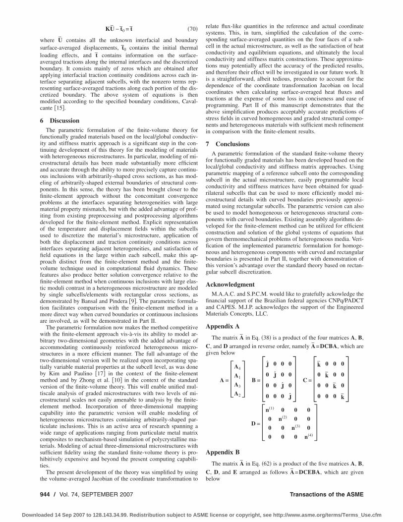
Appendix A

The matrix A in Eq. �38� is a product of the four matrices A, B,

C, and D arranged in reverse order, namely A=DCBA, which aregiven below

A = A4

A1

A3

A2

B = J 0 0 0

0 J 0 0

0 0 J 0

0 0 0 J C =

k 0 0 0

0 k 0 0

0 0 k 0

0 0 0 k

D = n�1� 0 0 0

0 n�2� 0 0

0 0 n�3� 0

0 0 0 n�4�

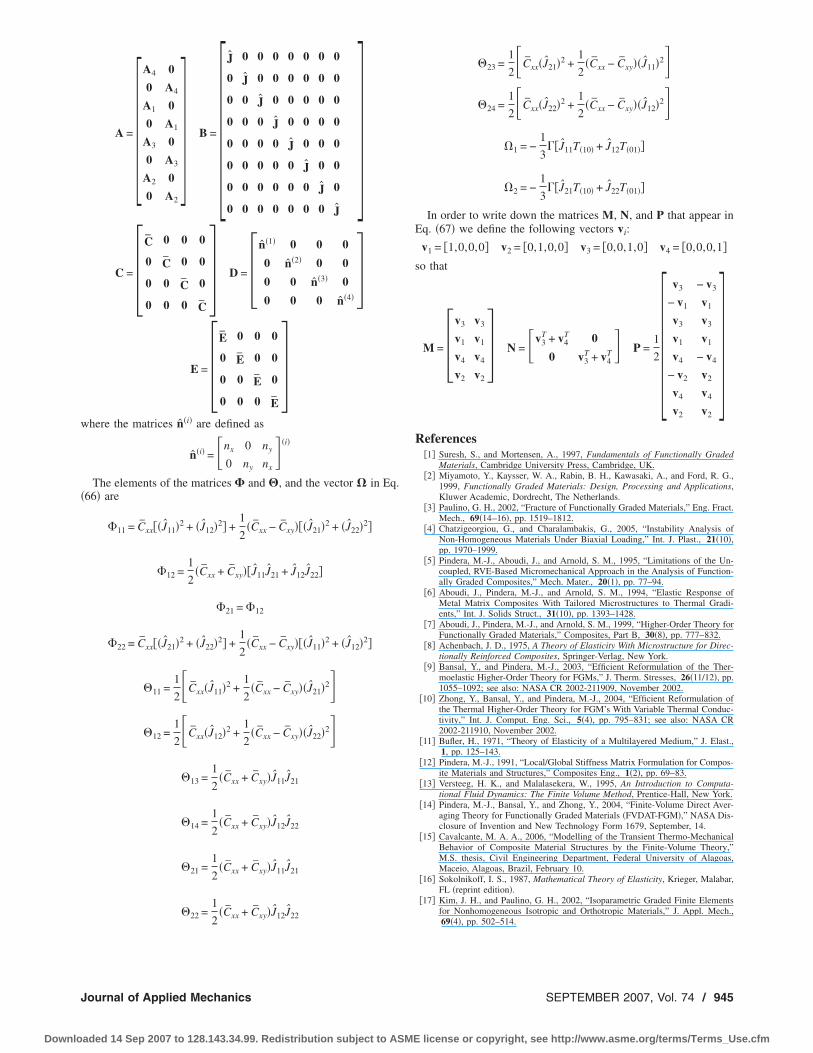
Appendix B

The matrix A in Eq. �62� is a product of the five matrices A, B,

C, D, and E arranged as follows A=DCEBA, which are given

Transactions of the ASME

license or copyright, see http://www.asme.org/terms/Terms_Use.cfm

w

�

J

Downlo

A = A4 0

0 A4

A1 0

0 A1

A3 0

0 A3

A2 0

0 A2

B = J 0 0 0 0 0 0 0

0 J 0 0 0 0 0 0

0 0 J 0 0 0 0 0

0 0 0 J 0 0 0 0

0 0 0 0 J 0 0 0

0 0 0 0 0 J 0 0

0 0 0 0 0 0 J 0

0 0 0 0 0 0 0 J

C =

C 0 0 0

0 C 0 0

0 0 C 0

0 0 0 C D =

n�1� 0 0 0

0 n�2� 0 0

0 0 n�3� 0

0 0 0 n�4�

E = E 0 0 0

0 E 0 0

0 0 E 0

0 0 0 E

here the matrices n�i� are defined as

n�i� = �nx 0 ny

0 ny nx��i�

The elements of the matrices and , and the vector � in Eq.66� are

�11 = Cxx��J11�2 + �J12�2� +1

2�Cxx − Cxy���J21�2 + �J22�2�

�12 =1

2�Cxx + Cxy��J11J21 + J12J22�

�21 = �12

�22 = Cxx��J21�2 + �J22�2� +1

2�Cxx − Cxy���J11�2 + �J12�2�

�11 =1

2�Cxx�J11�2 +

1

2�Cxx − Cxy��J21�2�

�12 =1

2�Cxx�J12�2 +

1

2�Cxx − Cxy��J22�2�

�13 =1

2�Cxx + Cxy�J11J21

�14 =1

2�Cxx + Cxy�J12J22

�21 =1

2�Cxx + Cxy�J11J21

�22 =1

�Cxx + Cxy�J12J22

ournal of Applied Mechanics

aded 14 Sep 2007 to 128.143.34.99. Redistribution subject to ASME

�23 =1

2�Cxx�J21�2 +

1

2�Cxx − Cxy��J11�2�

�24 =1

2�Cxx�J22�2 +

1

2�Cxx − Cxy��J12�2�

�1 = −1

3��J11T�10� + J12T�01��

�2 = −1

3��J21T�10� + J22T�01��

In order to write down the matrices M, N, and P that appear inEq. �67� we define the following vectors vi:

v1 = �1,0,0,0� v2 = �0,1,0,0� v3 = �0,0,1,0� v4 = �0,0,0,1�so that

M = v3 v3

v1 v1

v4 v4

v2 v2

N = �v3T + v4

T 0

0 v3T + v4

T � P =1

2v3 − v3

− v1 v1

v3 v3

v1 v1

v4 − v4

− v2 v2

v4 v4

v2 v2

References

�1� Suresh, S., and Mortensen, A., 1997, Fundamentals of Functionally GradedMaterials, Cambridge University Press, Cambridge, UK.

�2� Miyamoto, Y., Kaysser, W. A., Rabin, B. H., Kawasaki, A., and Ford, R. G.,1999, Functionally Graded Materials: Design, Processing and Applications,Kluwer Academic, Dordrecht, The Netherlands.

�3� Paulino, G. H., 2002, “Fracture of Functionally Graded Materials,” Eng. Fract.Mech., 69�14–16�, pp. 1519–1812.

�4� Chatzigeorgiou, G., and Charalambakis, G., 2005, “Instability Analysis ofNon-Homogeneous Materials Under Biaxial Loading,” Int. J. Plast., 21�10�,pp. 1970–1999.

�5� Pindera, M.-J., Aboudi, J., and Arnold, S. M., 1995, “Limitations of the Un-coupled, RVE-Based Micromechanical Approach in the Analysis of Function-ally Graded Composites,” Mech. Mater., 20�1�, pp. 77–94.

�6� Aboudi, J., Pindera, M.-J., and Arnold, S. M., 1994, “Elastic Response ofMetal Matrix Composites With Tailored Microstructures to Thermal Gradi-ents,” Int. J. Solids Struct., 31�10�, pp. 1393–1428.

�7� Aboudi, J., Pindera, M.-J., and Arnold, S. M., 1999, “Higher-Order Theory forFunctionally Graded Materials,” Composites, Part B, 30�8�, pp. 777–832.

�8� Achenbach, J. D., 1975, A Theory of Elasticity With Microstructure for Direc-tionally Reinforced Composites, Springer-Verlag, New York.

�9� Bansal, Y., and Pindera, M.-J., 2003, “Efficient Reformulation of the Ther-moelastic Higher-Order Theory for FGMs,” J. Therm. Stresses, 26�11/12�, pp.1055–1092; see also: NASA CR 2002-211909, November 2002.

�10� Zhong, Y., Bansal, Y., and Pindera, M.-J., 2004, “Efficient Reformulation ofthe Thermal Higher-Order Theory for FGM’s With Variable Thermal Conduc-tivity,” Int. J. Comput. Eng. Sci., 5�4�, pp. 795–831; see also: NASA CR2002-211910, November 2002.

�11� Bufler, H., 1971, “Theory of Elasticity of a Multilayered Medium,” J. Elast.,1, pp. 125–143.

�12� Pindera, M.-J., 1991, “Local/Global Stiffness Matrix Formulation for Compos-ite Materials and Structures,” Composites Eng., 1�2�, pp. 69–83.

�13� Versteeg, H. K., and Malalasekera, W., 1995, An Introduction to Computa-tional Fluid Dynamics: The Finite Volume Method, Prentice-Hall, New York.

�14� Pindera, M.-J., Bansal, Y., and Zhong, Y., 2004, “Finite-Volume Direct Aver-aging Theory for Functionally Graded Materials �FVDAT-FGM�,” NASA Dis-closure of Invention and New Technology Form 1679, September, 14.

�15� Cavalcante, M. A. A., 2006, “Modelling of the Transient Thermo-MechanicalBehavior of Composite Material Structures by the Finite-Volume Theory,”M.S. thesis, Civil Engineering Department, Federal University of Alagoas,Maceio, Alagoas, Brazil, February 10.

�16� Sokolnikoff, I. S., 1987, Mathematical Theory of Elasticity, Krieger, Malabar,FL �reprint edition�.

�17� Kim, J. H., and Paulino, G. H., 2002, “Isoparametric Graded Finite Elementsfor Nonhomogeneous Isotropic and Orthotropic Materials,” J. Appl. Mech.,

SEPTEMBER 2007, Vol. 74 / 945

license or copyright, see http://www.asme.org/terms/Terms_Use.cfm