EARTH SURFACE PROCESSES AND LANDFORMS … · EARTH SURFACE PROCESSES AND LANDFORMS Earth Surf. Process. Landforms 34, 848–859 ... 1 Department of Geography, Hydrogeography and Climatology

EARTH SURFACE PROCESSES AND LANDFORMSEarth Surf. Process. Landforms 34, 848–859 (2009)Copyright © 2009 John Wiley & Sons, Ltd.Published online 13 February 2009 in Wiley InterScience(www.interscience.wiley.com) DOI: 10.1002/esp.1779

John Wiley & Sons, Ltd.Chichester, UKESPEarth Surface Processes and LandformsEARTH SURFACE PROCESSES AND LANDFORMSEarth Surface Processes and LandformsThe Journal of the British Geomorphological Research GroupEarth Surf. Process. Landforms0197-93371096-9837Copyright © 2006 John Wiley & Sons, Ltd.John Wiley & Sons, Ltd.2006Earth ScienceEarth Science99999999ESP1779Research ArticleResearch ArticlesCopyright © 2006 John Wiley & Sons, Ltd.John Wiley & Sons, Ltd.2006

Spatial variability of rainfall on a sub-kilometre scaleSpatial variability of rainfall on a sub-kilometre scale

P. Fiener1* and K. Auerswald2

1 Department of Geography, Hydrogeography and Climatology Research Group, Universität zu Köln, Cologne, Germany 2 Lehrstuhl für Grünlandlehre, Technische Universität München, Freising-Weihenstephan, Germany

Received 6 March 2008; Revised 31 October 2008; Accepted 12 November 2008

* Correspondence to: P. Fiener, Department of Geography, Hydrogeography and Climatology Research Group, Universität zu Köln, Albertus Magnus Platz, D-50923Cologne, Germany. E-mail: [email protected]

ABSTRACT: The variability of rainfall in space and time is an essential driver of many processes in nature but little is knownabout its extent on the sub-kilometre scale, despite many agricultural and environmental experiments on this scale. A network of13 tipping-bucket rain gauges was operated on a 1·4 km2 test site in southern Germany for four years to quantify spatial trends inrainfall depth, intensity, erosivity, and predicted runoff. The random measuring error ranged from 10% to 0·1% in case of 1 mmand 100 mm rainfall, respectively. The wind effects could be well described by the mean slope of the horizon at the stations.Except for one station, which was excluded from further analysis, the relative differences due to wind were in maximum ±5%.Gradients in rainfall depth representing the 1-km2 scale derived by linear regressions were much larger and ranged from 1·0 to15·7 mm km–1 with a mean of 4·2 mm km–1 (median 3·3 mm km–1). They mainly developed during short bursts of rain and thusgradients were even larger for rain intensities and caused a variation in rain erosivity of up to 255% for an individual event. Thetrends did not have a single primary direction and thus level out on the long term, but for short-time periods or for single eventsthe assumption of spatially uniform rainfall is invalid on the sub-kilometre scale. The strength of the spatial trend increased withrain intensity. This has important implications for any hydrological or geomorphologic process sensitive to maximum rainintensities, especially when focusing on large, rare events. These sub-kilometre scale differences are hence highly relevant forenvironmental processes acting on short-time scales like flooding or erosion. They should be considered during establishing,validating and application of any event-based runoff or erosion model. Copyright © 2009 John Wiley & Sons, Ltd.

KEYWORDS: rainfall variability; rain intensity variability; runoff; rainfall measurement

Introduction

The variability of rainfall in space and time is an essential driverof many processes in nature. This is most obvious for questionssuch as the analysis and modelling of rainfall–runoff relations(e.g. Bronstert and Bárdossy, 2003; Faurès et al., 1995; Kirkbyet al., 2005) or soil erosion processes (e.g. Nyssen et al., 2005;Nearing, 1998), but it is also important for characteristicssuch as spatial-temporal variability of crop yields, patterns ofdeposits from atmosphere, soil carbon and nitrogen turnover,etc.

Spatial variability of rainfall on a scale >100 km2 has beenan important topic in hydrology and meteorology researchduring the last decades. Studies focused on methods toimprove the interpolation of rain gauge point measurements(e.g. Syed et al., 2003; Borga and Vizzaccaro, 1997; Kruizingaand Yperlaan, 1978), optimizing rain gauge networks (e.g.Papamichail and Metaxa, 1996; Bastin et al., 1984), or utilizingremote sensing data, especially ground-based radar measure-ments (e.g. Borga, 2002; Datta et al., 2003; Quirmbach andSchultz, 2002; Tsanis et al., 2002; Berne et al., 2004), todetermine the spatial variability of rainfall. On smaller scales

(10–100 km2) studies are rarer and test sites are mostly locatedin areas where strong gradients in rainfall can be expected dueto orographic effects in mountainous regions (e.g. Buytaertet al., 2006; Arora et al., 2006) or at coast lines (e.g. Stowand Dirks, 1998), or due to climatic situations with distinctconvective storms (e.g. Desa and Niemczynowicz, 1997;Hernandez et al., 2000; Berne et al., 2004).

On a smaller scale (<10 km2), where many environmentalprocesses are often studied in detail and where rainfall–runoffor erosion models are mostly developed and tested only sparseknowledge exists on the variability of rainfall depth andintensity (e.g. Goodrich et al., 1995; Jensen and Pedersen,2005; Taupin, 1997; Sivakumar and Hatfield, 1990). Informationis needed about the extent and significance of rain variabilityon this scale, for example to develop and validate erosionand rainfall–runoff models (e.g. Faurès et al., 1995; Johannes,2001), to understand small-scale variability in soil moistureand hence soil properties, to design urban water managementfacilities (e.g. Berne et al., 2004), or to validate subscalevariability in rain radar data (e.g. Jensen and Pedersen, 2005).

The overall aim of this study was to determine the spatialvariability in rainfall depth and maximum intensity, as well as

Copyright © 2009 John Wiley & Sons, Ltd. Earth Surf. Process. Landforms, Vol. 34, 848–859 (2009)DOI: 10.1002/esp

SPATIAL VARIABILITY OF RAINFALL ON A SUB-KILOMETRE SCALE 849

variability of derived parameters within a small test site(1·4 km2) with 13 measuring stations. More specifically theobjectives were to:

(i) Determine the importance of spatially variable eventsduring the four-year observation period.

(ii) Analyse the extent of spatial variability for the total raindepth and the maximum intensities on an event basis.

(iii) Analyse the resulting spatial variability of parametersnon-linearly related to rainfall, exemplarily shown forrainfall erosivity and predicted daily runoff.

Material and Methods

Test site

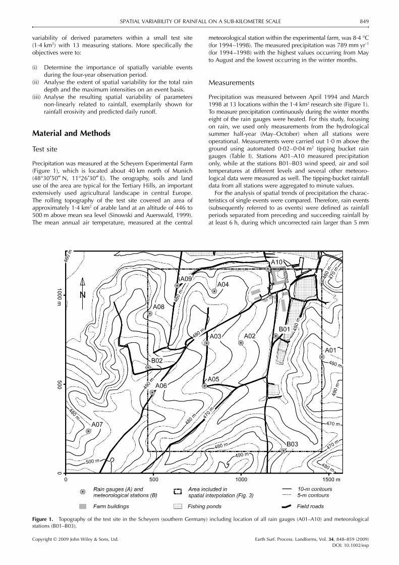
Precipitation was measured at the Scheyern Experimental Farm(Figure 1), which is located about 40 km north of Munich(48°30′50″ N, 11°26′30″ E). The orography, soils and landuse of the area are typical for the Tertiary Hills, an importantextensively used agricultural landscape in central Europe.The rolling topography of the test site covered an area ofapproximately 1·4 km2 of arable land at an altitude of 446 to500 m above mean sea level (Sinowski and Auerswald, 1999).The mean annual air temperature, measured at the central

meteorological station within the experimental farm, was 8·4 °C(for 1994–1998). The measured precipitation was 789 mm yr–1

(for 1994–1998) with the highest values occurring from Mayto August and the lowest occurring in the winter months.

Measurements

Precipitation was measured between April 1994 and March1998 at 13 locations within the 1·4 km² research site (Figure 1).To measure precipitation continuously during the winter monthseight of the rain gauges were heated. For this study, focusingon rain, we used only measurements from the hydrologicalsummer half-year (May–October) when all stations wereoperational. Measurements were carried out 1·0 m above theground using automated 0·02–0·04 m2 tipping bucket raingauges (Table I). Stations A01–A10 measured precipitationonly, while at the stations B01–B03 wind speed, air and soiltemperatures at different levels and several other meteoro-logical data were measured as well. The tipping-bucket rainfalldata from all stations were aggregated to minute values.

For the analysis of spatial trends of precipitation the charac-teristics of single events were compared. Therefore, rain events(subsequently referred to as events) were defined as rainfallperiods separated from preceding and succeeding rainfall byat least 6 h, during which uncorrected rain larger than 5 mm

Figure 1. Topography of the test site in the Scheyern (southern Germany) including location of all rain gauges (A01–A10) and meteorologicalstations (B01–B03).


850 EARTH SURFACE PROCESSES AND LANDFORMS

was measured at Station B01, B02 or 50% of all stations, thisis analogous to the definition of an erosive event by Wischmeierand Smith (1978).

To identify erroneous measurements and to prevent persistentfailure of single stations, e.g. due to insects, leaves, etc. trappedin the collecting funnel of the tipping buckets, observed raindepths and characteristics were controlled monthly. Moreover,the event durations at the different stations were compared toidentify stations with prolonged rain events often indicating aplugged collecting funnel. In the case of any suspicious findingsin the data the equipment of the identified station waschecked and the measurements were rejected if necessary.

As known from a number of studies the accuracy of tippingbucket rain gauges is sensitive to rain intensity, which wascompensated either by correction functions (e.g. Adami andDa Deppo, 1986; Molini et al., 2005; La Barbera et al., 2002)or by improving measuring techniques (e.g. Overgaard et al.,1998). For this study three of the tipping bucket rain gaugeswere tested under different rain intensities in the laboratoryto derive intensity dependent correction functions. For rainintensities <30 mm h–1, which represent more than 90% of allmeasured rain events at the test site, no significant relation-ship between rain intensity and measuring error could befound. However, larger tendencies than those measured inthe laboratory experiments can be expected due to a slightfouling of equipment installed for field measurements. Thetipping bucket error of the field measurements was determinedby collecting the rain water intercepted by the gauges in smalltanks buried below ground level near the measuring device.These small tanks were emptied bi-weekly to determine totalrain depth which was used to correct the tipping bucket data.Both measurements were closely correlated at all 13 stations(R2 > 0·998), nevertheless a deviation of the tipping bucketmeasurements between –7% to +8% was found (mean absolutedeviation being 3%). The station-dependent relation was usedto adjust the tipping bucket data with individual correctionfactors ranging between 0·927 (A06) and 1·081 (B03).

Quantifying spatial variability due to wind effects

Using rain gauges at a height of 1 m above ground causes windeffects which result in differences between measured rainand actual rain reaching the surface. These differences wereinvestigated with additional surface-level rain gauges at themeteorological stations B01 and B02 (Johannes, 2001). For

this study dealing with the spatial distribution of rain depthand intensity it is important to focus on differences in windeffects between the 13 rain stations. Such differences can beexpected due to different measuring devices and differentwind effects mainly caused by different slopes of the horizonat the measuring locations (Table I). To detect wind effectswe firstly categorized all events in: (i) events with spatiallyrandom variability in rainfall distribution and (ii) events withspatially systematic variability in rainfall distribution (see nextsub-section).

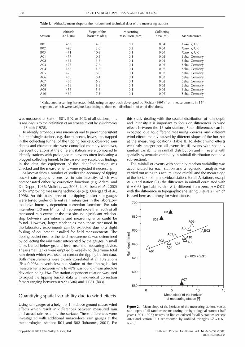
The rainfall of events with spatially random variability wasaccumulated for each station and a regression analysis wascarried out using this accumulated rainfall and the mean slopeof the horizon of the individual station. For all A-stations, exceptA07, and station B03 the difference in rainfall correlated withR2 = 0·63 (probability that R is different from zero, p = 0·01)with the difference in topographic sheltering (Figure 2), whichis used here as a proxy for wind effects.

Table I. Altitude, mean slope of the horizon and technical data of the measuring stations

StationAltitude a.s.l. (m)

Slope of the horizona (deg)

Measuring resolution (mm)

Collectingarea (m²) Manufacturer

B01 453 4·8 0·2 0·04 Casella, UKB02 496 3·0 0·2 0·04 Casella, UKB03 471 10·9 0·1 0·04 Casella, UKA01 477 0·5 0·1 0·02 Seba, GermanyA02 465 3·8 0·1 0·02 Seba, GermanyA03 475 7·6 0·1 0·02 Seba, GermanyA04 466 4·5 0·1 0·02 Seba, GermanyA05 470 8·0 0·1 0·02 Seba, GermanyA06 486 8·4 0·1 0·02 Seba, GermanyA07 485 6·9 0·1 0·02 Seba, GermanyA08 468 8·9 0·1 0·02 Seba, GermanyA09 456 5·6 0·1 0·02 Seba, GermanyA10 460 7·3 0·1 0·02 Seba, Germany

a Calculated assuming harvested fields using an approach developed by Richter (1995) from measurements in 15°segments, which were weighted according to the mean distribution of wind directions.

Figure 2. Mean slope of the horizon of the measuring stations versusrain depth of all random events during the hydrological summer-halfyears (1994–1997); regression line calculated for all A-stations (exceptA07) and station B03 represented by unfilled triangles (R2 = 0·63,n = 9).



The rain depth at the individual A-stations deviated by notmore than 2% from the average of all A-stations (excluding A07)if total rain of all random events was accumulated. At A07,however, the rainfall of all random events was 11% smalleron average compared to all other A-stations. This significantdifference (two-sided t-test; null hypothesis mean of all A-stations equal to mean of station A07) was probably causedby higher wind speeds due to the location of A07 in a smalldepression canalizing wind coming from south and south-west,which are the dominant wind directions of the area (representing59·2% of all wind directions). At stations B01 and B02 themeasured rain decreased less with increasing wind speedthan at the A-stations (inclusive B03). In total 5% more rain thanthe average of all A-stations (except A07, inclusive B03) wasmeasured for all events during the hydrological summer-halfyear. The major reason probably was the aerodynamically moreappropriate design of the B01 and B02 rain gauges with aslightly different slope of the rim of these two stations (Johannes,2001).

When analysing the wind effects at the stations B01 and B02,where additional surface-level rain gauges were installed, wefound a larger measuring error at B02 for accumulated rainfall(1994–1998) of 7% compared to 5% at station B01. Thisdifference can be attributed to higher average wind speedsof 2·3 m s–1 at B02 compared to those of 1·3 m s–1 at B01.Nevertheless, the analysis of single rain events did not allowa clear relationship to be derived between wind speed andmeasuring error for each of the stations, because the sizeof the errors also depended strongly on rain characteristics.In general, the relative error decreased with increasing eventsize, for example all events <10 mm had a relative error of9·0%, while this decreased to 4·2% for all larger events.

The average wind speed during all events with spatiallysystematic variability [1·7 m s–1, standard deviation (SD) =0·3 m s–1] was significantly lower compared to the spatiallyrandom events (2·4 m s–1, SD = 1·3 m s–1) (two-tailed t-test,null hypothesis is equality of means). Hence, as we focuson rainfall events with a spatially systematic variability, nocorrections for wind speed were applied due to the totalrelatively small random error caused by wind effects in thecase of these events and the general difficulties to derive clearcorrection functions. Only measurements from station A07were excluded from further evaluations due to its specificsensitivity to wind speed. If we use or refer to average raindepths these are calculated according to the Thiessen polygonareas varying between 4·7 and 18·5 ha for the individualstations (excluding A07) within the rectangle stretched by themeasuring locations shown in Figure 1.

Defining spatially random and spatially systematic variability in rainfall distribution

To distinguish between events, where the spatial variation ofrain was random due to measuring errors and those eventswith a spatially systematic variability, a multiple regressionanalysis was performed, applying a linear, an exponential ora polynomial function. For these regression models, usingrain depth regressed on X–Y-coordinates of the stations, thenull hypothesis that the coefficients of the model (exceptfor intercept) were different from zero was tested applyingt-statistics. Events are defined as events with a spatiallysystematic variability in rainfall distribution (subsequentlyreferred to as gradient events) if one of the model coefficientsor the total regression model is highly significant (p < 0·01). Ifthe null hypothesis holds not true on this significance levelthe events were categorized as events with a spatially random

variability in rainfall distribution (subsequently referred toas random events). The residuals of the gradient events werethen tested for normal distribution and autocorrelation (seelater) to examine whether the regression model was appropriateto describe the spatial trend.

To illustrate and discuss the spatial variability of rainfall eventswithin the research area without a predefined spatial model,geostatistical analyses [for theory see Webster and Oliver (2000)and Nielsen and Wendroth (2003)] were carried out for fourexemplary gradient events. Semivariograms were constructedwith the supplementary package geoR (Diggle and Ribeiro Jr,2007) of the statistical software GNU R, version 2·6 (RDevelopment Core Team, 2007). For semivariance analysis raingauge readings of all four gradient events were pooled (Voltzand Webster, 1990) to meet the requirement of at least 30–50 data sets (n = 48). According to Schuurmans et al. (2007) apooled semivariogram is almost as good as using event-basedsemivariograms. Prior to pooling, the data of the individualrains were scaled to a mean of zero and a standard deviationof one to attain second order stationarity among rains. Thisresulted in an empirical semivariogram, which closely followeda Gaussian model (nugget 0·06, sill 5·09, range 1333 m, Nash–Sutcliffe index 0·9356) where 12 lag classes were weightedaccording to n/lag when fitting the semivariogram model togive more weight to those lag classes, which contained manydata pairs and which were closer to the origin and thus moreimportant for kriging. The small nugget effect and the large sillindicated a strong pattern of the rains compared to theuncertainty. This semivariogram model and the scaled data ofthe individual rains were then used to construct rain maps byblock kriging using 10 × 10 m2 blocks with the package gstat(Pebesma, 2004), which were finally rescaled to millimetre unitswith the mean and standard deviation of the individual rains.

Analysis of the regressions, analysis of the residuals and theexemplarily geostatistically interpolated rain maps (Figure 3),all indicated that the resulting gradient events generallyfollowed a more or less linear trend. Hence, rain depth wasthen linearly regressed on the X–Y-coordinates of the stationsto determine the mean trend for each gradient event, whichlater on is used for an easy comparison and further analysis ofthe resulting trends. Analogously to the spatial interpolationof the four exemplary gradient events a semivariogram wascalculated by pooling all gradient events prior and aftercorrecting for the trend by regression analysis to examine towhich degree the linear regression equations with predefinedspatial behaviour adequately quantified and removed thespatial trend and how much autocorrelation was left in theresiduals of the regression analysis.

Parameters derived from rainfall – rain erosivity and runoff prediction

To elucidate the effects of spatial gradient events on environ-mental processes at the sub-kilometre scale it is necessary tofocus on driving parameters derived form rainfall depth, whichmay translate rainfall variability sub- or super-proportional tothe respective process. As an example for such a parameterthe rain erosivity was calculated, which is commonly usedto describe the rain potential to detach soil particles and toinitiate soil erosion caused by surface runoff. Rain erosivityoriginally was introduced with the Universal Soil Loss Equation(USLE; Wischmeier and Smith, 1960) and now it is used inmany soil erosion models. Rain erosivity Re is calculatedaccording to Equation 1 for all erosive events, defined asevents with at least 10 mm of precipitation or a maximumintensity above 10 mm h–1 (Schwertmann et al., 1987).



Re = E × Imax30 (1)

(2)

with:

Ei = ((11·89 + (8·73 log Ii)) Ni 10−3 for 0·05 ≤ Ii ≤ 76·2

Ei = 0 for Ii < 0·05

Ei = 28·33 Ni 10−3 for Ii > 76·2

where E is the total kinetic energy of an event (in kJ m–2),Imax30 is the maximum 30-min rain intensity of an event (inmm h–1), i is a time interval during the event with a constantrain intensity, Ei, Ii, and Ni are kinetic energy, rain intensityand accumulation within time interval i, respectively.

In addition daily runoff was calculated for the days withgradient rains applying the Soil Conservation Service (SCS)curve number model (Mockus, 1972). Two contrastingsituations on Hydrological Soil Group C were assumed,either small grain favouring infiltration (curve number 81) orrow crops more likely favouring runoff (curve number 85)

E Eii

n

==∑

1

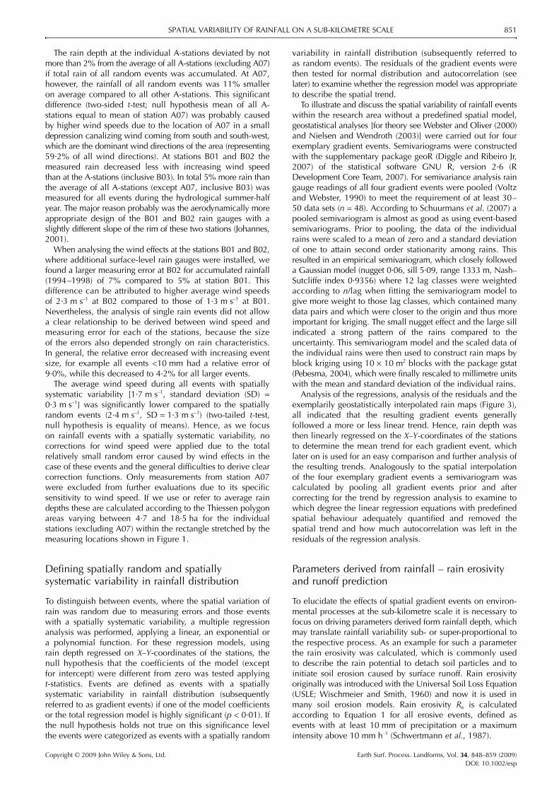
Figure 3. Interpolation of rain depth (in mm) of four gradient events by block kriging for 10 × 10-m2 blocks; the twelve locations of themeasuring stations (A01–A06, A08–A10, B01–B03) are indicated by grey circles; for each four events its duration, average rain depth (AVR rain)calculated from the geostatistical interpolation and average gradients in rain depth (AVR gradient) are given. Krige standard deviations averagedover all 10 × 10-m2 blocks are 0·4, 0·5, 0·9 and 1·1 mm for rains 8, 64, 71 and 116, respectively.



which both corresponded to the land use on the experimentalfarm (Fiener and Auerswald, 2007).

Results

In total 115 events ≥ 5·0 mm were observed in the four hydrolo-gical summer-half years (1994–1997). These events weremeasured at least at eight of the 13 measuring stations (includingA07). In case of 52 events all 13 stations were operating. Onaverage between 2·5 (October) and 6·8 events (August) permonth occurred during the observation period. These eventsrepresent 67% (September) to 90% (July) of the total rainamount in these months. The largest rainfall was 62·2 mm,while the mean and the median of all events in the hydrologicalsummer-half years were 12·6 mm and 9·3 mm, respectively.

When applying the multiple regressions to determinegradient events, the linear, exponential and polynomialmodels showed similar levels of significance and similar R2

values. The curvilinear regression surfaces were with fewexceptions not significantly [tested according to Samiuddin(1970)] better than the linear model. This justified using alinear trend for further analysis in addition to the definition ofscale associated with the linear model. Also the geostatisticalinterpolation examples (Figure 3) justified the use of a lineartrend. For 38 events during the hydrological summer-half yearthe linear regression was at least highly significant (p < 0·01).The R2 for the linear regressions ranged between 0·59 and0·96, with 50% of all R2 > 0·81. Geostatistical analysis of

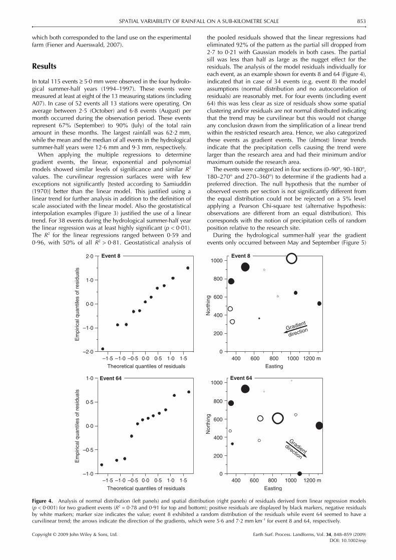
the pooled residuals showed that the linear regressions hadeliminated 92% of the pattern as the partial sill dropped from2·7 to 0·21 with Gaussian models in both cases. The partialsill was less than half as large as the nugget effect for theresiduals. The analysis of the model residuals individually foreach event, as an example shown for events 8 and 64 (Figure 4),indicated that in case of 34 events (e.g. event 8) the modelassumptions (normal distribution and no autocorrelation ofresiduals) are reasonably met. For four events (including event64) this was less clear as size of residuals show some spatialclustering and/or residuals are not normal distributed indicatingthat the trend may be curvilinear but this would not changeany conclusion drawn from the simplification of a linear trendwithin the restricted research area. Hence, we also categorizedthese events as gradient events. The (almost) linear trendsindicate that the precipitation cells causing the trend werelarger than the research area and had their minimum and/ormaximum outside the research area.

The events were categorized in four sections (0–90°, 90–180°,180–270° and 270–360°) to determine if the gradients had apreferred direction. The null hypothesis that the number ofobserved events per section is not significantly different fromthe equal distribution could not be rejected on a 5% levelapplying a Pearson Chi-square test (alternative hypothesis:observations are different from an equal distribution). Thiscorresponds with the notion of precipitation cells of randomposition relative to the research site.

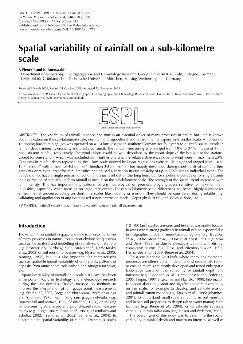
During the hydrological summer-half year the gradientevents only occurred between May and September (Figure 5)

Figure 4. Analysis of normal distribution (left panels) and spatial distribution (right panels) of residuals derived from linear regression models(p < 0·001) for two gradient events (R2 = 0·78 and 0·91 for top and bottom); positive residuals are displayed by black markers, negative residualsby white markers; marker size indicates the value; event 8 exhibited a random distribution of the residuals while event 64 seemed to have acurvilinear trend; the arrows indicate the direction of the gradients, which were 5·6 and 7·2 mm km–1 for event 8 and 64, respectively.



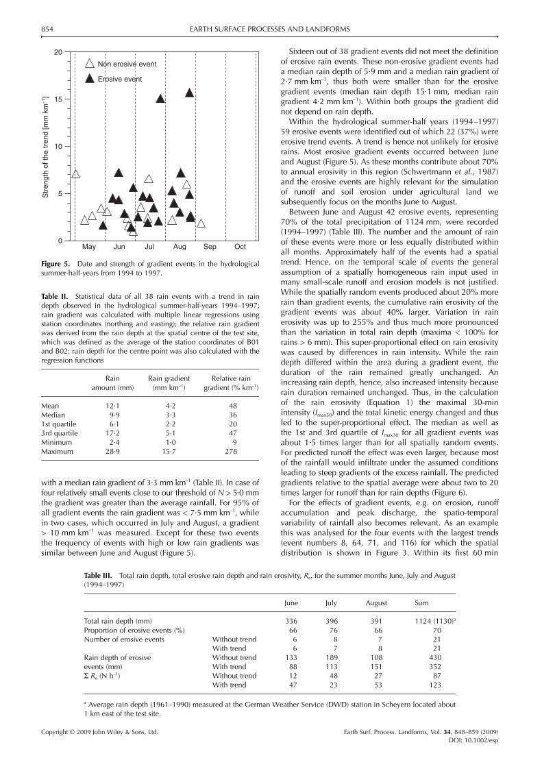
with a median rain gradient of 3·3 mm km–1 (Table II). In case offour relatively small events close to our threshold of N > 5·0 mmthe gradient was greater than the average rainfall. For 95% ofall gradient events the rain gradient was < 7·5 mm km–1, whilein two cases, which occurred in July and August, a gradient> 10 mm km–1 was measured. Except for these two eventsthe frequency of events with high or low rain gradients wassimilar between June and August (Figure 5).

Sixteen out of 38 gradient events did not meet the definitionof erosive rain events. These non-erosive gradient events hada median rain depth of 5·9 mm and a median rain gradient of2·7 mm km–1, thus both were smaller than for the erosivegradient events (median rain depth 15·1 mm, median raingradient 4·2 mm km–1). Within both groups the gradient didnot depend on rain depth.

Within the hydrological summer-half years (1994–1997)59 erosive events were identified out of which 22 (37%) wereerosive trend events. A trend is hence not unlikely for erosiverains. Most erosive gradient events occurred between Juneand August (Figure 5). As these months contribute about 70%to annual erosivity in this region (Schwertmann et al., 1987)and the erosive events are highly relevant for the simulationof runoff and soil erosion under agricultural land wesubsequently focus on the months June to August.

Between June and August 42 erosive events, representing70% of the total precipitation of 1124 mm, were recorded(1994–1997) (Table III). The number and the amount of rainof these events were more or less equally distributed withinall months. Approximately half of the events had a spatialtrend. Hence, on the temporal scale of events the generalassumption of a spatially homogeneous rain input used inmany small-scale runoff and erosion models is not justified.While the spatially random events produced about 20% morerain than gradient events, the cumulative rain erosivity of thegradient events was about 40% larger. Variation in rainerosivity was up to 255% and thus much more pronouncedthan the variation in total rain depth (maxima < 100% forrains > 6 mm). This super-proportional effect on rain erosivitywas caused by differences in rain intensity. While the raindepth differed within the area during a gradient event, theduration of the rain remained greatly unchanged. Anincreasing rain depth, hence, also increased intensity becauserain duration remained unchanged. Thus, in the calculationof the rain erosivity (Equation 1) the maximal 30-minintensity (Imax30) and the total kinetic energy changed and thusled to the super-proportional effect. The median as well asthe 1st and 3rd quartile of Imax30 for all gradient events wasabout 1·5 times larger than for all spatially random events.For predicted runoff the effect was even larger, because mostof the rainfall would infiltrate under the assumed conditionsleading to steep gradients of the excess rainfall. The predictedgradients relative to the spatial average were about two to 20times larger for runoff than for rain depths (Figure 6).

For the effects of gradient events, e.g. on erosion, runoffaccumulation and peak discharge, the spatio-temporalvariability of rainfall also becomes relevant. As an examplethis was analysed for the four events with the largest trends(event numbers 8, 64, 71, and 116) for which the spatialdistribution is shown in Figure 3. Within its first 60 min

Figure 5. Date and strength of gradient events in the hydrologicalsummer-half-years from 1994 to 1997.

Table II. Statistical data of all 38 rain events with a trend in raindepth observed in the hydrological summer-half-years 1994–1997;rain gradient was calculated with multiple linear regressions usingstation coordinates (northing and easting); the relative rain gradientwas derived from the rain depth at the spatial centre of the test site,which was defined as the average of the station coordinates of B01and B02; rain depth for the centre point was also calculated with theregression functions

Rain amount (mm)

Rain gradient(mm km–1)

Relative rain gradient (% km–1)

Mean 12·1 4·2 48Median 9·9 3·3 361st quartile 6·1 2·2 203rd quartile 17·2 5·1 47Minimum 2·4 1·0 9Maximum 28·9 15·7 278

Table III. Total rain depth, total erosive rain depth and rain erosivity, Re, for the summer months June, July and August(1994–1997)

June July August Sum

Total rain depth (mm) 336 396 391 1124 (1130)a

Proportion of erosive events (%) 66 76 66 70Number of erosive events Without trend 6 8 7 21

With trend 6 7 8 21Rain depth of erosive events (mm)

Without trend 133 189 108 430With trend 88 113 151 352

Σ Re (N h–1) Without trend 12 48 27 87With trend 47 23 53 123

a Average rain depth (1961–1990) measured at the German Weather Service (DWD) station in Scheyern located about1 km east of the test site.



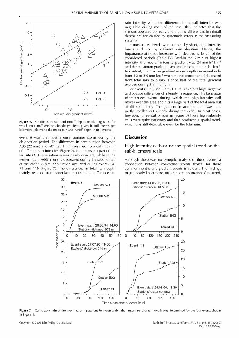
event 8 was the most intense summer storm during theobservation period. The difference in precipitation betweenA06 (22 mm) and A01 (29·1 mm) resulted from only 15 minof different rain intensity (Figure 7). In the eastern part of thetest site (A01) rain intensity was nearly constant, while in thewestern part (A06) intensity decreased during the second halfof the event. A similar situation occurred during events 64,71 and 116 (Figure 7). The differences in total rain depthmainly resulted from short-lasting (<30 min) differences in

rain intensity while the difference in rainfall intensity wasnegligible during most of the rain. This indicates that thestations operated correctly and that the differences in rainfalldepths are not caused by systematic errors in the measuringsystems.

In most cases trends were caused by short, high intensitybursts and not by different rain duration. Hence, theimportance of trends increases with decreasing length of theconsidered periods (Table IV). Within the 5 min of highestintensity, the median intensity gradient was 24 mm h–1 km–1

and the maximum gradient even amounted to 49 mm h–1 km–1.In contrast, the median gradient in rain depth decreased onlyfrom 4·2 to 2·0 mm km–1 when the reference period decreasedfrom total rain to 5 min. Hence half of the total gradientevolved during 5 min of rain.

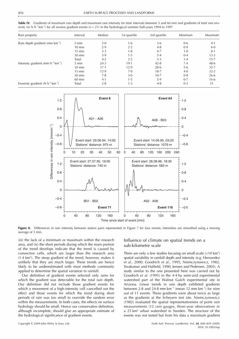
For event 8 (29 June 1994) Figure 8 exhibits large negativeand positive differences of intensity in sequence. This behaviourcharacterizes events during which the high-intensity cellmoves over the area and hits a large part of the total area butat different times. The gradient in accumulation was thuspartly levelled out already during the event. In most cases,however, (three out of four in Figure 8) these high-intensitycells were quite stationary and thus produced a spatial trend,which was still detectable even for the total rain.

Discussion

High-intensity cells cause the spatial trend on the sub-kilometre scale

Although there was no synoptic analysis of these events, aconnection between convective storms typical for thesesummer months and gradient events is evident. The findingsof (i) a nearly linear trend, (ii) a random orientation of the trend,

Figure 6. Gradients in rain and runoff depths (excluding rains, forwhich no runoff was predicted); gradients given in millimetres perkilometre relative to the mean rain and runoff depth in millimetres.

Figure 7. Cumulative rain of the two measuring stations between which the largest trend of rain depth was determined for the four events shownin Figure 3.



(iii) the lack of a minimum or maximum within the researcharea, and (iv) the short periods during which the main portionof the trend develops indicate that the trend is caused byconvective cells, which are larger than the research area(1·4 km2). The steep gradient of the trend, however, makes itunlikely that they are much larger. These trends are hencelikely to be underestimated with most methods commonlyapplied to determine the spatial variation in rainfall.

Our definition of gradient events selected only rains forwhich the gradient was detectable for the total rain depth.Our definition did not include those gradient events forwhich a movement of a high-intensity cell cancelled out theeffect and those events for which the trend during shortperiods of rain was too small to override the random errorwithin the measurements. In both cases, the effects on surfacehydrology should be small. Hence our conservative definition,although incomplete, should give an appropriate estimate ofthe hydrological significance of gradient events.

Influence of climate on spatial trends on a sub-kilometre scale

There are only a few studies focusing on small-scale (<10 km2)spatial variability in rainfall depth and intensity (e.g. Hernandezet al., 2000; Goodrich et al., 1995; Niemczynowicz, 1982;Sivakumar and Hatfield, 1990; Jensen and Pedersen, 2005). Astudy similar to the one presented here was carried out byGoodrich et al. (1995) in the 4·4 ha semi-arid experimentalwatershed part of the Walnut Gulch experimental site inArizona. Linear trends in rain depth exhibited gradientsbetween 2·8 and 24·8 mm km–1 (mean 12 mm km–1) for nineout of 11 events. These gradients were about twice as largeas the gradients at the Scheyern test site. Niemczynowicz(1982) evaluated the spatial representativeness of point rainmeasurements (12 rain gauges, three-year observation) ina 25 km2 urban watershed in Sweden. The structure of theevents was not tested but from his data a maximum gradient

Table IV. Gradients of maximum rain depth and maximum rain intensity for time intervals between 5 and 60 min and gradients of total rain ero-sivity (in N h–1 km–1) for all erosive gradient events (n = 21) in the hydrological summer half-years 1994 to 1997

Rain property Interval Median 1st quartile 3rd quartile Minimum Maximum

Rain depth gradient (mm km–1) 5 min 2·0 1·6 3·6 0·6 4·110 min 2·9 2·2 4·8 0·9 6·015 min 3·3 1·8 4·7 1·0 8·130 min 3·9 1·5 5·4 0·4 13·3Total 4·2 2·5 5·3 1·4 15·7

Intensity gradient (mm h–1 km–1) 5 min 24·3 19·1 42·8 7·4 48·610 min 17·1 12·9 28·6 5·6 35·715 min 12·9 7·0 18·7 4·0 32·230 min 7·8 3·0 10·7 0·8 26·660 min 4·1 1·5 5·9 0·7 16·6

Erosivity gradient (N h–1 km–1) Total 2·8 1·3 4·8 0·3 31

Figure 8. Differences in rain intensity between station pairs represented in Figure 7 for four events; intensities are smoothed using a movingaverage of 3 min.



of 5·5 mm km–1 can be derived, which is only one-third of themaximum gradient found at Scheyern (15·7 mm km–1). Thus,the gradients seem to increase from the maritime Swedishsituation to the sub-continental Scheyern climate and furtherto the semi-arid, continental climate in Arizona.

Sub-kilometre scale spatial trends increase with storm size and recurrence interval

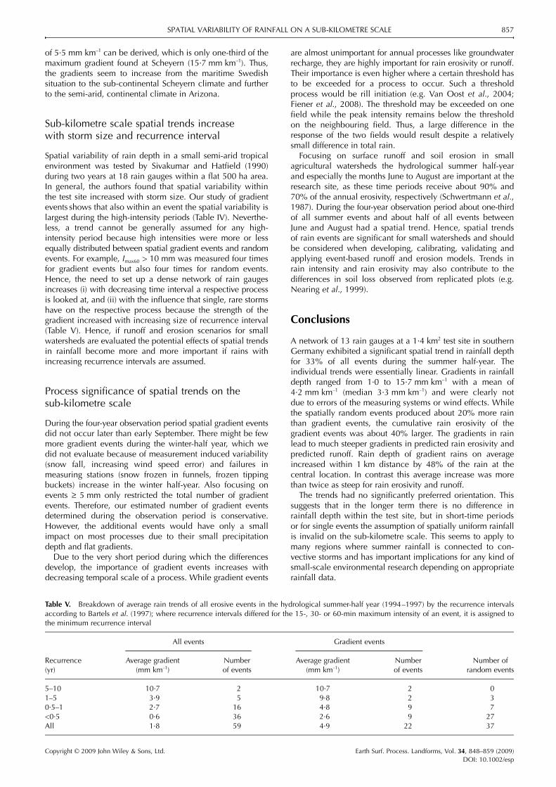
Spatial variability of rain depth in a small semi-arid tropicalenvironment was tested by Sivakumar and Hatfield (1990)during two years at 18 rain gauges within a flat 500 ha area.In general, the authors found that spatial variability withinthe test site increased with storm size. Our study of gradientevents shows that also within an event the spatial variability islargest during the high-intensity periods (Table IV). Neverthe-less, a trend cannot be generally assumed for any high-intensity period because high intensities were more or lessequally distributed between spatial gradient events and randomevents. For example, Imax60 > 10 mm was measured four timesfor gradient events but also four times for random events.Hence, the need to set up a dense network of rain gaugesincreases (i) with decreasing time interval a respective processis looked at, and (ii) with the influence that single, rare stormshave on the respective process because the strength of thegradient increased with increasing size of recurrence interval(Table V). Hence, if runoff and erosion scenarios for smallwatersheds are evaluated the potential effects of spatial trendsin rainfall become more and more important if rains withincreasing recurrence intervals are assumed.

Process significance of spatial trends on the sub-kilometre scale

During the four-year observation period spatial gradient eventsdid not occur later than early September. There might be fewmore gradient events during the winter-half year, which wedid not evaluate because of measurement induced variability(snow fall, increasing wind speed error) and failures inmeasuring stations (snow frozen in funnels, frozen tippingbuckets) increase in the winter half-year. Also focusing onevents ≥ 5 mm only restricted the total number of gradientevents. Therefore, our estimated number of gradient eventsdetermined during the observation period is conservative.However, the additional events would have only a smallimpact on most processes due to their small precipitationdepth and flat gradients.

Due to the very short period during which the differencesdevelop, the importance of gradient events increases withdecreasing temporal scale of a process. While gradient events

are almost unimportant for annual processes like groundwaterrecharge, they are highly important for rain erosivity or runoff.Their importance is even higher where a certain threshold hasto be exceeded for a process to occur. Such a thresholdprocess would be rill initiation (e.g. Van Oost et al., 2004;Fiener et al., 2008). The threshold may be exceeded on onefield while the peak intensity remains below the thresholdon the neighbouring field. Thus, a large difference in theresponse of the two fields would result despite a relativelysmall difference in total rain.

Focusing on surface runoff and soil erosion in smallagricultural watersheds the hydrological summer half-yearand especially the months June to August are important at theresearch site, as these time periods receive about 90% and70% of the annual erosivity, respectively (Schwertmann et al.,1987). During the four-year observation period about one-thirdof all summer events and about half of all events betweenJune and August had a spatial trend. Hence, spatial trendsof rain events are significant for small watersheds and shouldbe considered when developing, calibrating, validating andapplying event-based runoff and erosion models. Trends inrain intensity and rain erosivity may also contribute to thedifferences in soil loss observed from replicated plots (e.g.Nearing et al., 1999).

Conclusions

A network of 13 rain gauges at a 1·4 km2 test site in southernGermany exhibited a significant spatial trend in rainfall depthfor 33% of all events during the summer half-year. Theindividual trends were essentially linear. Gradients in rainfalldepth ranged from 1·0 to 15·7 mm km–1 with a mean of4·2 mm km–1 (median 3·3 mm km–1) and were clearly notdue to errors of the measuring systems or wind effects. Whilethe spatially random events produced about 20% more rainthan gradient events, the cumulative rain erosivity of thegradient events was about 40% larger. The gradients in rainlead to much steeper gradients in predicted rain erosivity andpredicted runoff. Rain depth of gradient rains on averageincreased within 1 km distance by 48% of the rain at thecentral location. In contrast this average increase was morethan twice as steep for rain erosivity and runoff.

The trends had no significantly preferred orientation. Thissuggests that in the longer term there is no difference inrainfall depth within the test site, but in short-time periodsor for single events the assumption of spatially uniform rainfallis invalid on the sub-kilometre scale. This seems to apply tomany regions where summer rainfall is connected to con-vective storms and has important implications for any kind ofsmall-scale environmental research depending on appropriaterainfall data.

Table V. Breakdown of average rain trends of all erosive events in the hydrological summer-half year (1994–1997) by the recurrence intervalsaccording to Bartels et al. (1997); where recurrence intervals differed for the 15-, 30- or 60-min maximum intensity of an event, it is assigned tothe minimum recurrence interval

All events Gradient events

Recurrence(yr)

Average gradient(mm km–1)

Number of events

Average gradient(mm km–1)

Numberof events

Number of random events

5–10 10·7 2 10·7 2 01–5 3·9 5 9·8 2 30·5–1 2·7 16 4·8 9 7<0·5 0·6 36 2·6 9 27All 1·8 59 4·9 22 37



The strength of the spatial trend was not related to rain depthbut increased with rain intensity. The trends thus also increasedin strength with recurrence interval. Moreover, the gradientsof maximum intensities were more pronounced compared tothose of rain depth. This has important implications for anyhydrological or geomorphologic process sensitive to maximumrain intensities, especially when focusing on large, rare events.As an example shown for rain erosivity, relative gradients ofderived environmental parameters can be much steeper thanthose of rain depth or intensity. Hence, it will take considerablylonger until sub-kilometre scale differences in such parameterslevel out than the time needed to level out difference inrain depth. These farm-scale differences are highly relevantfor environmental processes acting on short-time scales likeflooding or erosion. They should be considered during estab-lishing, validating and application of any event-based erosion(or hydrological) model.

Acknowledgements—The scientific activities of the research network‘Forschungsverbund Agrarökosysteme München’ (FAM) were financiallysupported by the German Federal Ministry of Education and Research(BMBF 0339370). Overhead costs of the research station of Scheyernwere funded by the Bavarian State Ministry for Science, Research andArts. The continuous technical supervision and maintenance of thestations was carried out by Richard Wenzel and Bernhard Johannes.The help with statistical analyses by Bernhard Johannes, Max Wittmerand Josef Nipper is gratefully acknowledged. The actual research is partof the German Research Agency (DFG) project DI 639/1-1 (Markus Disse).

References

Adami A, Da Deppo L. 1986. On the Systematic Errors of TippingBucket Recording Rain Gauges. Proceedings of the Correction ofPrecipitation Measurements. ETH/IAHS/WMO workshop on thecorrection of precipitation measurements, Zürich; 27–30.

Arora M, Singh P, Goel NK, Singh RD. 2006. Spatial distributionand seasonal variability of rainfall in a mountainous basin inthe Himalayan region. Water Resources Management 20: 489–508. DOI: 10.1007/s11269-006-8773-4

Bartels H, Malitz G, Asmus S, Albrecht FM, Dietzer B, Günther T,Ertel H. 1997. Starkniederschlaghöhen für Deutschland – KOSTRA[Recurrence time of rain intensities – KOSTRA] DeutscherWetterdienst: Offenbach a. Main (in German).

Bastin G, Lorent B, Duque C, Gevers M. 1984. Optimal estimation ofthe average areal rainfall and optimal selection of rain-gaugelocations. Water Resources Research 20: 463–470.

Berne A, Delrieu G, Creutin JD, Obled C. 2004. Temporal and spatialresolution of rainfall measurements required for urban hydrology.Journal of Hydrology 299: 166–179.

Borga M. 2002. Accuracy of radar rainfall estimates for streamflowsimulation. Journal of Hydrology 267: 26–39.

Borga M, Vizzaccaro A. 1997. On the interpolation of hydrologicvariables: formal equivalence of multiquadratic surface fitting andkriging. Journal of Hydrology 195: 160–171.

Bronstert A, Bárdossy A. 2003. Uncertainty of runoff modelling atthe hillslope scale due to temporal variations of rainfall intensity.Physics and Chemistry of the Earth 28: 283–288.

Buytaert W, Celleri R, Willems P, De Bievre B, Wyseure G. 2006.Spatial and temporal rainfall variability in mountainous areas: acase study from the south Ecuadorian Andes. Journal of Hydrology329: 413–421.

Datta S, Jones WL, Roy B, Tokay A. 2003. Spatial variability ofsurface rainfall as observed from TRMM field campaign data. Journalof Applied Meteorology 42: 598–610.

Desa MNM, Niemczynowicz J. 1997. Dynamics of short rainfall stormsin a small scale urban area in Coly Limper, Malaysia. AtmosphericResearch 44: 293–315.

Diggle PJ, Ribeiro Jr PJ. 2007. Model-based Geostatistics. Springer:New York.

Faurès J-M, Goodrich DC, Woolhiser DA, Sorooshian S. 1995.Impact of small-scale spatial rainfall variability on runoff modeling.Journal of Hydrology 173: 309–326.

Fiener P, Auerswald K. 2007. Rotation effects of potato, maize andwinter wheat on soil erosion by water. Soil Science Society ofAmerica Journal 71: 1919–1925.

Fiener P, Govers G, Van Oost K. 2008. Evaluation of a dynamicmulti-class sediment transport model in a catchment under soil-conservation agriculture. Earth Surface Processes and Landforms33: 1639–1660.

Goodrich DC, Faures JM, Woolhiser DA, Lane LJ, Sorooshian S.1995. Measurement and analysis of small-scale convective stormrainfall variability. Journal of Hydrology 173: 283–308.

Hernandez M, Miller SN, Goodrich DC, Goff BF, Kepner WG,Edmonds CM, Jones KB. 2000. Modeling runoff response to landcover and rainfall spatial variability in semi-arid watersheds.Environmental Monitoring and Assessment 64: 285–298.

Jensen NE, Pedersen L. 2005. Spatial variability of rainfall:variations within a single radar pixel. Atmospheric Research 77:269–277.

Johannes B. 2001. Ausmaß und Ursachen kleinräumiger Nieder-Schlagsvariabilität und Konzequenzen für die Abflussbildung[Extend and Cause of Spatial Rain Variability in Small Areas –Effects on Surface Runoff], FAM-Bericht 50. Shaker: Aachen (inGerman).

Kirkby MJ, Bracken LJ, Shannon J. 2005. The influence of rainfalldistribution and morphological factors on runoff delivery fromdryland catchments in SE Spain. Catena 62: 136–156.

Kruizinga S, Yperlaan GJ. 1978. Spatial interpolation of daily totals ofrainfall. Journal of Hydrology 36: 65–73.

La Barbera P, Lanza LG, Stagi L. 2002. Tipping bucket mechanicalerrors and their influence on rainfall statistics and extremes. WaterScience and Technology 45: 1–9.

Mockus V. 1972. Estimation of direct runoff from storm rainfall. InSCS National Engineering Handbook. Section 4. Hydrology. USDA:Washington, DC.

Molini A, Lanza LG, La Barbera P. 2005. Improving the accuracyof tipping-bucket rain records using disaggregation techniques.Atmospheric Research 77: 203–217.

Nearing MA. 1998. Why soil erosion models over-predict small soillosses and under-predict large soil losses. Catena 32: 15–22.

Nearing MA, Govers G, Norton DL. 1999. Variability in soil erosiondata from replicated plots. Soil Science Society of America Journal63: 1829–1835.

Nielsen DR, Wendroth O. 2003. Spatial and Temporal Statistics:Sampling Field Soils and their Vegetation. Catena Verlag:Cremmlingen.

Niemczynowicz J. 1982. Areal intensity–duration–frequency curvesfor short-term rainfall events in Lund. Nordic Hydrology 13: 193–204.

Nyssen J, Vandenreyken H, Poesen J, Moeyersons J, Deckers J, HaileM, Salles C, Govers G. 2005. Rainfall erosivity and variability inthe Northern Ethiopian Highlands. Journal of Hydrology 311: 172–187.

Overgaard S, El-Shaarawi AH, Arnbjerg-Nielsen K. 1998. Calibrationof tipping bucket rain gauges. Water Science and Technology 37:139–145.

Papamichail DM, Metaxa IG. 1996. Geostatistical analysis of spatialvariability of rainfall and optimal design of a rain gauge network.Water Resources Management 10: 107–127. DOI: 10.1007/BF00429682

Pebesma EJ. 2004. Multivariable geostatistics in S: the gstat package.Computers & Geosciences 30: 683–691.

Quirmbach M, Schultz GA. 2002. Comparison of rain gauge andradar data as input to an urban rainfall–runoff model. WaterScience and Technology 45: 27–33.

R Development Core Team. 2007. R: a language and environmentfor statistical computing. http://www.R-project.org [Accessed 20September 2007].

Richter D. 1995. Ergebnisse methodischer Untersuchungen zur Korrekturdes systematischen Meßfehlers des Hellmann-Niederschlagsmessers[Analysis of Methods to Correct Systematic Errors of Hellmann RainGauges]. DWD Offenbach Selbstverlag: Offenbach (in German).

http://www.R-project.org

10.1007/s11269-006-8773-4

10.1007/BF00429682



Samiuddin M. 1970. On a test for an assigned value of correlation ina bivariate normal distribution. Biometrika 57: 461–464.

Schuurmans JM, Bierkens MFP, Pebesma EJ, Uijlenhoet R. 2007.Automatic prediction of high-resolution daily rainfall fields formultiple extents: the potential of operational radar. Journal ofHydrometeorology 8: 1204–1224.

Schwertmann U, Vogl W, Kainz M. 1987. Bodenerosion durchWasser – Vorhersage des Abtrags und Bewertung von Gegenmaßnah-men [Soil Erosion by Water – Prediction of Soil Loss and Valuationof Counter-measures]. Ulmer Verlag: Stuttgart (in German).

Sinowski W, Auerswald K. 1999. Using relief parameters in adiscriminant analysis to stratify geological areas with differentspatial variability of soil properties. Geoderma 89: 113–128.

Sivakumar MVK, Hatfield JL. 1990. Spatial variability of rainfall at anexperimental station in Niger, West Africa. Theoretical and AppliedClimatology 42: 33–39. DOI: 10.1007/BF00865524

Stow CD, Dirks KN. 1998. High-resolution studies of rainfall onNorfolk Island: Part 1. The spatial variability of rainfall. Journal ofHydrology 208: 163–186.

Syed KH, Goodrich DC, Myers DE, Sorooshian S. 2003. Spatialcharacteristics of thunderstorm rainfall fields and their relation torunoff. Journal of Hydrology 271: 1–21.

Taupin JD. 1997. Characterization of rainfall spatial variability at ascale smaller than 1 km in a semiarid area (region of Niamey,Niger). Comptes Rendus de l Academie des Sciences Serie IiFascicule A-Sciences de la Terre et des Planetes 325: 251–256.

Tsanis IK, Gad MA, Donaldson NT. 2002. A comparative analysis ofrain-gauge and radar techniques for storm kinematics. Advances inWater Resources 25: 305–316.

Van Oost K, Beuselinck L, Hairsine PB, Govers G. 2004. Spatialevaluation of multi-class sediment transport and depositon model.Earth Surface Processes and Landforms 29: 1027–1044.

Voltz M, Webster R. 1990. A comparison of kriging, cubic splinesand classification for predicting soil properties from sampleinformation. Journal of Soil Science 41: 473–490.

Webster R, Oliver MA. 2000. Geostatistics for EnvironmentalScientists. John Wiley & Sons: Chichester.

Wischmeier WH, Smith DD. 1960. A Universal Soil-loss Equation toGuide Conservation Farm Planning. International Society of SoilScience: Madison, WI.

Wischmeier WH, Smith DD. 1978. Predicting Rainfall Erosion Losses– A Guide to Conservation Planning. US Government Print Office:Washington, DC.

10.1007/BF00865524

EARTH SURFACE PROCESSES AND LANDFORMS … · EARTH SURFACE PROCESSES AND LANDFORMS Earth Surf. Process. Landforms 34, 848–859 ... 1 Department of Geography, Hydrogeography and Climatology

Documents