Dynamical Casimir effect and quantum cosmology

OKHEP–00–01

Dynamical Casimir Effect and Quantum Cosmology

I. Brevik†

Division of Applied Mechanics, Norwegian University

of Science and Technology, N-7491 Trondheim, Norway

K. A. Milton‡

Department of Physics and Astronomy,

The University of Oklahoma, Norman, OK 73019, USA

S.D. Odintsov§ and K.E. Osetrin∗∗

Department of Mathematics and Physics,

Tomsk State Pedagogical University, Tomsk 634041, Russia

(Dated: May 12, 2000)

Abstract

We apply the background field method and the effective action formalism to describe the four-

dimensional dynamical Casimir effect. Our picture corresponds to the consideration of quantum

cosmology for an expanding FRW universe (the boundary conditions act as a moving mirror) filled

by a quantum massless GUT which is conformally invariant. We consider cases in which the static

Casimir energy is attractive and repulsive. Inserting the simplest possible inertial term, we find,

in the adiabatic (and semiclassical) approximation, the dynamical evolution of the scale factor and

the dynamical Casimir stress analytically and numerically (for SU(2) super Yang-Mills theory).

Alternative kinetic energy terms are explored in the Appendix.

PACS numbers: 04.60.-m, 11.15.Kc, 12.10.-g, 12.60.Jv

†Electronic address: [email protected]‡Electronic address: [email protected]; URL: http://www.nhn.ou.edu/%7Emilton/§Electronic address: [email protected],[email protected]; Present address: Insti-

tuto de Fısica de la Universidad de Guanajuato, 37150 Leon, Mexico∗∗Electronic address: [email protected]

1

2

1. INTRODUCTION

The Casimir effect [1] can be regarded as the change in the zero-point fluctuations dueto nontrivial boundary conditions. Surveys of the effect are given, for instance, by Plunienet al. [2], Mostepanenko and Trunov [3], and Milton [4]. The recent “resource letter” ofLamoreaux [5] contains a wealth of references, although it is admittedly highly incomplete.

In the past, the Casimir effect has been considered as a static effect. Growing interestin recent years has been drawn to the dynamical variant of the effect, meaning, in essence,that not only the geometrical configurations of the external boundaries (such as plates) butalso their velocities play a physical role. Moore [6] is probably the first to have consideredthe dynamical Casimir effect. Examples of more recent references are [7] and [8].

The recent paper of Nagatani and Shigetomi [9] is an interesting development in thisdirection. These authors focused attention on the fact that if moving boundaries (mirrors)create radiation, the mirrors have to experience a reaction force. They proposed an effectivetheory for the back reaction of the dynamical Casimir effect in (1+1) dimensions for a scalarfield, this theory being constructed by the background field method in the path integralformalism. In fact, they considered a kind of 2d quantum cosmology for describing thedynamical Casimir effect.

In the present paper we show how to apply the effective action formalism, using thebackground field method, to formulate the dynamical Casimir effect in four dimensions in aconvenient and elegant form. We are able to consider an arbitrary matter content (typicallya grand unified theory or GUT) and present the dynamical Casimir effect as a kind ofquantum cosmological model. Using the background field method, we treat the geometricalconfiguration of the boundaries classically, but consider the GUT in the interior region as aquantum object.

In the next section we consider a GUT in a three-dimensional space, where the sizeof the space a(t) is a dynamical variable. Similarly to [9] we make use of the adiabaticapproximation. Exploiting the conformal invariance of the theory we calculate the anomaly-induced effective action W . In the simplest case (a torus), W is given by Eq. (2.4). Weconsider the static Casimir energy in section 3, and show that, for the usual boundaryconditions on the torus, the Casimir energy is attractive. In section 4 we start with theeffective action, Eq. (4.1), for the dynamical case. Introducing a mass m associated with thescale factor a, with a corresponding kinetic energy in the low-velocity approximation equalto 1

2ma2 (a phenomenological term), we then consider two cases. If the Casimir energy

is attractive, we derive in Eq. (4.15) the time variation of a(t) for large values of t, thelast term in the expression being a (special case of the) dynamical correction to the purequasistatic Casimir result. For the perhaps less realistic repulsive case, the small and largetime behavior of the Casimir behavior is extracted in Eqs. (4.24), (4.26). Numerical resultsin both cases are given in Section 5. The behavior of the scale factor in the two cases isshown in Figs. 1 and 3, while the dynamical stress on the torus is presented in Figs. 2 and4. In the Appendix we discuss the effects of alternative kinetic energy terms.

3

2. THE EFFECTIVE ACTION

Let us consider conformally invariant, massless matter in 4d-dimensional space-time. Thematter may correspond to some GUT (say, SU(5), SO(10), or any other alternative). Weare interested first in the study of the static Casimir effect for such a theory when the fieldis assumed to be bounded in a three-dimensional region. In other words, we are interestedin a space having the form R

1 ⊗K3, where as K3 one can take any manifold permitting anexact Casimir effect calculation. It can be S

3, T3, S

1 ⊗ S2 or any other compact manifold

with a known spectrum of the d’Alembertian operator. We limit ourselves to T3 or S

3, forthe sake of simplicity.

Suppose now that our GUT lives in such a three-dimensional space, where the size ofthe space is a dynamical variable (moving mirror or moving universe). Hence, we willbe interested in the dynamical Casimir effect in a three-dimensional region and the back-reaction from the induced radiation on the moving background geometry. We shall use theadiabatic approximation in this study. A great simplification comes from adopting a physicalpicture in which the Casimir effect is described as an effective action in curved spacetime(see [10] for an introduction). Here, spacetime is taken to be an expanding universe withtopology R

1 ⊗ S3 or R

1 ⊗ T3. The corresponding metric is given by

ds2 = dt2 − a2(t)ds23, (2.1)

where ds23 = dx2 + dy2 + dz2 for T

3 (coordinates are restricted by all radii being equal), orthe line element of a three-dimensional sphere S

3.Let us calculate now the effective action for such a GUT. Using the fact that the theory

is conformally invariant we may use the anomaly-induced effective action [11]:

W = b

∫

d4x√−gF σ

+ b′∫

d4x√−g {σ[22

2+ 4Rµν∇µ∇ν −

4

3R 2 +

2

3(∇µR)(∇µ)]σ + (G− 2

32 R)σ}

− 1

12× 2

3(b + b′)

∫

d4x√−g[R− 62σ − 6(∇µσ)(∇µσ)]2, (2.2)

where our metric is presented in conformal form. Thus gµν = e2σgµν , σ = ln a(η), η is theconformal time, F is the square of the Weyl tensor, and G is the square of the Gauss-Bonnetinvariant. Overbar quantities indicate that the calculation is made with gµν . Further,

b =1

120(4π)2(N0 + 6N1/2 + 12N1),

b′ = − 1

360(4π)2(N0 + 11N1/2 + 62N1), (2.3)

where N0, N1/2, and N1 are the numbers of scalars, spinors, and vectors. For example, for

N = 4 SU(N) super YM one gets [12] b = −b′ = (N2 − 1) [4(4π)2]−1

. We also adopt thescheme wherein the b′′-coefficient of the 2R term in the conformal anomaly is zero. Beingambiguous, it does not influence the dynamics [12].

4

As the simplest case we consider henceforth a torus. Then

W =

∫

dη[

2b′σσ′′′′ − 2(b + b′)(σ′′ + σ′2)2]

. (2.4)

This is a typical effective action for a GUT in a Friedman-Robertson-Walker (FRW) Universeof a special form.

3. THE STATIC CASIMIR ENERGY

Let us briefly overview the static Casimir effect for a torus of side L (for more detail, see[13]). The Casimir energies associated with massless spin-j fields is

ENj=

Nj

2(−1)2j

∑

n∈Z3

ωn,j, (3.1)

where we see the appearance of the characteristic minus sign associated with a closed Fermionloop. The frequency of each mode is given by

ω2n,j =

(

2π

L

)2 3∑

i=1

(ni + g(j)i )2, n = (n1, n2, n3), (3.2)

Here g(j)i = 0, 1/2 depending on the field type chosen in R

1 ⊗ T3.

We use the p-dimensional Epstein zeta function Zp

∣

∣

∣

∣

g1, . . . , gp

h1, . . . , hp

∣

∣

∣

∣

(s) defined for < s > 1

by the formula

Zp

∣

∣

∣

∣

g1, . . . , gp

h1, . . . , hp

∣

∣

∣

∣

(s) =∑

n∈Zp

′[

(n1 + g1)2 + ... + (np + gp)

2]−ps/2

× exp [2πi(n1h1 + ... + nphp)] , (3.3)

where gi and hi are real numbers, and the prime means omitting the term with (n1, ..., np) =(−g1, ...,−gp) if all the gi are integers. For < s < 1 the Epstein function is understood tobe the analytic continuation of the right-hand side of Eq. (3.3). Defined in such a way, theEpstein zeta function obeys the functional equation

π−ps/2Γ

(

1

2ps

)

Zp

∣

∣

∣

∣

g1, . . . , gp

h1, . . . , hp

∣

∣

∣

∣

(s) = π−p(1−s)/2Γ

(

1

2p(1− s)

)

× exp [−2πi(g1h1 + ... + gphp)] Zp

∣

∣

∣

∣

h1, . . . , hp

−g1, . . . , −gp

∣

∣

∣

∣

(1− s), (3.4)

The function (3.3) is an entire function in the complex s plane except for the case when allhi are integers. In the latter case the function (3.3) has a simple pole at s = 1.

Using Eq. (3.3) we have

ENj=

π

LNj(−1)2jZ3

∣

∣

∣

∣

g(j)1 g

(j)2 g

(j)3

0 0 0

∣

∣

∣

∣

(

−1

3

)

. (3.5)

5

Taking into account the functional equation (3.4) one gets

Z3

∣

∣

∣

∣

g(j)1 g

(j)2 g

(j)3

0 0 0

∣

∣

∣

∣

(

−1

3

)

= − 1

2π3Z3

∣

∣

∣

∣

0 0 0

−g(j)1 −g

(j)2 −g

(j)3

∣

∣

∣

∣

(

4

3

)

. (3.6)

The Casimir energies (3.1) take the form

ENj= −(−1)2j

2π2LNjZ3

∣

∣

∣

∣

0 0 0

−g(j)1 −g

(j)2 −g

(j)3

∣

∣

∣

∣

(

4

3

)

. (3.7)

Finally the Casimir energy associated with a multiplet of fields characterized by the numbersN0, N1/2, and N1 can be written as follows

E =∑

j

ENj= − 1

2π2L

[

N0Z3

∣

∣

∣

∣

0 0 0

−g(0)1 −g

(0)2 −g

(0)3

∣

∣

∣

∣

(

4

3

)

−N1/2Z3

∣

∣

∣

∣

0 0 0

−g(1/2)1 −g

(1/2)2 −g

(1/2)3

∣

∣

∣

∣

(

4

3

)

+ N1Z3

∣

∣

∣

∣

0 0 0

−g(1)1 −g

(1)2 −g

(1)3

∣

∣

∣

∣

(

4

3

)]

. (3.8)

Thus, the static Casimir energy for a torus is proportional to c/L, where c is defined by thefeatures of the GUT under consideration. Note that the sign of c is a priori unpredictable.

If for all the fields of the theory we take the same boundary conditions (periodic orantiperiodic), the Z3’s are all equal, and consequently the supersymmetry is not broken,and the Casimir energy is zero. On the other hand, if the different fields satisfy differenttypes of boundary conditions, supersymmetry is broken and there is a static Casimir effect.

For the latter situation, consider, as an illustration, the usual case of bosons satisfying pe-riodic boundary conditions and fermions satisfying antiperiodic boundary conditions on thetorus. Then we require only two values. For the bosons, the Casimir energy is proportionalto

Z3

∣

∣

∣

∣

0 0 00 0 0

∣

∣

∣

∣

(

4

3

)

= 16.5323, (3.9)

which value is given explicitly in Ref. [14]. For the fermions, the same reference gives thevalue

Z3

∣

∣

∣

∣

0 0 012

12

12

∣

∣

∣

∣

(

4

3

)

= −3.86316. (3.10)

So each term in Eq. (3.8) contributes a negative energy. Thus the net Casimir energy isattractive,

E = − c

L, c = 0.837537(N0 + N1) + 0.195710N1/2 = 1.033247N1/2, (3.11)

since the number of fermions must be equal to the number of bosons.1

1Any case with periodic boundary conditions in some directions and antiperiodic ones in others may be

given in terms of the values given in Eqs. (3.9), (3.10) and the additional values

Z3

∣

∣

∣

∣

∣

0 0 01

20 0

∣

∣

∣

∣

∣

(

4

3

)

= 0.689223, Z3

∣

∣

∣

∣

∣

0 0 01

2

1

20

∣

∣

∣

∣

∣

(

4

3

)

= −2.156887.

6

We should make the following general remarks concerning the physical interpretation ofthe calculation sketched here. Imposition of periodic boundary conditions at the boundariesof the field volume is a basic physical ingredient in expressions such as Eqs. (3.1), (3.2) for theCasimir energy. It is analogous to the imposition of perfect conducting boundary conditions,or more generally, electromagnetic boundary conditions, at the walls, when consideringordinary electrodynamics, for example within a spherical volume. The physical outcome ofa calculation of this kind is the residual energy remaining when the influence of the localstresses is separated off. (Presumably, such stresses are absorbed in a kind of renormalizationof physical parameters.) The field theoretical calculation is able to cope only with the cutoffindependent part of the physical stress; the local cutoff dependent parts of the stress areautomatically lost in the zeta-function regularization process. This is an important pointwhenever the result of the field theoretical calculation is to be compared with experiments.

As a typical example of this sort, we may mention the calculation of the Casimir energyof a dilute dielectric ball. One may adopt a field theoretical viewpoint (cf., for instance,[15]), from which the Casimir energy is calculated as a cutoff independent, positive, ex-pression. More detailed considerations, using quantum mechanical perturbation theory [16](cf. also [17]), or quantum statistical mechanics [18] show however how this expression isto be supplemented with attractive cutoff dependent parts. Such terms are presumably notobservable. As for the cutoff independent term, agreement between the methods is found,so the situation is in this respect satisfactory.

4. DYNAMICAL PROPERTIES

Now let us turn to a simplified discussion of the dynamical Casimir effect. We here takeinto account that we have a dynamical radius a(t)L, a(t) being a dimensionless scale factor.Then, the total effective action is given as

Γ = W − L

∫

dη a(η) E , (4.1)

where W is given by Eq. (2.4) and E = −c/(aL) as displayed in Eq. (3.8). Because theaction is dimensionless, the length L disappears from the calculation, and we have

Γ =

∫

dη[

2b′σσ′′′′ − 2(b + b′)(σ′′ + σ′2)2 + c]

. (4.2)

This is a typical effective action to describe a quantum FRW Universe.In order to consider dynamical properties we add to the above effective action a phe-

nomenological term, which has the form of a kinetic energy. We associate a mass m withthe scale factor a, and take the corresponding kinetic energy to be given by 1

2ma2. Our es-

sential idea is that the geometrical configuration of the space is treated classically and thatthe GUT field is a quantum object which induces the Casimir effect. One might in principleintroduce other expressions for the kinetic energy, but this expression is clearly the simplestchoice that one can make. The Newtonian form is moreover in correspondence with our useof the adiabatic approximation, meaning that |a(t)| � 1; cf. also the analogous argument

7

in [9] in connection with the (1+1) dimensional case.2 Introducing the physical time t viadη/dt = 1/a, we now write Γ as

Γ =

∫

dt

[

1

2ma2 + 2b′ ln a (

....a a2 + 3

...a aa + a2a + aa2)

− 2(b + b′)(a2 + aa)2

a+

c

a

]

, (4.3)

where a = da/dt.From the variational equation δΓ/δa = 0 we obtain, after some algebra,3

ma− 2 b′(

a2 + 2d2

dt2(aa)

)

− 2 (b + b′)

(

2a....a +4a

...a +3a2 − 12

a2a

a+ 3

a4

a2

)

+c

a2= 0. (4.4)

It is remarkable that the the logarithm is absent in Eq. (4.4); there seems to be no reasona priori why this should be so.

We limit ourselves to the N = 4 SU(N) super YM theory for which, as mentioned,(b + b′) = 0. Then Eq. (4.4) simplifies to

ma + 2b(2....a a + 4

...a a + 3a2) +

c

a2= 0. (4.5)

Both the terms involving b and c are dynamical, quantum mechanical, effects, which indimensional terms are proportional to ~. However, we will see that it is sensible (if c 6= 0)to regard the b term as a small correction to the Casimir-determined geometry. We denotethe b = 0 solution by a0(t); it satisfies the equation

ma0 +c

a20

= 0, (4.6)

implying

1

2ma2

0 =c

a0

+ const. (4.7)

2We consider other possibilities for the kinetic energy term in the Appendix.3This and subsequent equations are dimensionally consistent if we restore dimensions:

[a] = [t] = [m−1] = Length.

8

4.1 Attractive Casimir energy, c > 0

If the Casimir energy is attractive, as actually realized in our illustrative calculation givenin Sec. 3, see Eq. (3.11), we will assume, as boundary conditions, that a0(t → ∞) = ∞,a0(t → ∞) = 0. Then, the constant in Eq. (4.7) becomes equal to zero, and we get theCasimir solution

a0(t) = At2

3 , with A =

(

9c

2m

)1

3

. (4.8)

It is worth noticing here that the proportionality of a0(t) to t2/3 is precisely the behaviourshown by the scale factor in the Einstein-de Sitter universe. This may be surprising atfirst sight, but does not seem to be so unreasonable after all, since the Einstein-de Sitteruniverse is flat, thus in correspondence with our neglect of Riemannian curvature terms inthe formalism above.

Now we turn to the solution a(t), taking into account the b correction. We shall limitourselves to giving a perturbative solution, implying an expansion of a(t) around a0(t)assuming b to be small:

a(t) = a0(t) + ba1(t). (4.9)

We consider only times for which the correction term is small:

ba1/a0 � 1. (4.10)

Thus, we may expand the Casimir term in Eq. (4.5) as c/a2 = (c/a20)(1− 2ba1/a0). A first

order expansion of the other terms in Eq. (4.5) then yields, when we take into account theCasimir solution (4.8), the inhomogeneous equation

a1 −4

9t2a1 =

8A2

9mt−

8

3 . (4.11)

The homogeneous version of Eq. (4.11) has solutions of the form tα, with α = 4/3 andα = −1/3. We write the independent solutions as

f(t) = t4

3 , g(t) = t−1

3 . (4.12)

The Wronskian ∆ between f and g is simple; ∆ = f g − gf = −5/3. Writing for brevitythe right hand side of Eq. (4.11) as r we then get, as the solution of the inhomogeneousequation,

a1(t) = f(t)

(

C1 −1

∆

∫

rg dt

)

+ g(t)

(

C2 +1

∆

∫

rf dt

)

= t4

3

(

C1 −4A2

15mt−2

)

+ t−1

3

(

C2 +8A2

5mt−

1

3

)

= C1t4/3 + C2t

−1/3 +4

3

A2

mt−2/3, (4.13)

9

with C1 and C2 being constants. As for the values of these constants, we have first to observeour restriction (4.10), which implies that

b

A

(

C1t2

3 + C2t−1 +

4A2

3mt−

4

3

)

� 1. (4.14)

If we require the perturbative approximation to be valid for large times, we must haveC1 = 0. If we also set C2 = 0, our perturbative solution becomes

a(t) = At2

3 +4A2

3mbt−

2

3 , (4.15)

which is only valid for large enough t, i.e., for

bA

mt−

4

3 � 1. (4.16)

The static Casimir force is

FCas = − ∂

∂a

(

− c

a

)

= − c

a2, (4.17)

whereas the dynamical force is

Fdyn = ma. (4.18)

Substituting Eq. (4.15) into Eqs. (4.17) and (4.18), and observing the relation between cand A in Eq. (4.8), we get

Fdyn = FCas

(

1− 4bA

mt−4/3

)

, (4.19)

which shows that the dynamical force is the Casimir force modified by a small dynamicalcorrection when the perturbative approximation is valid.

Before we turn to a numerical solution of Eq. (4.5), we discuss the repulsive case.

4.2 Repulsive Casimir energy, c < 0

Now let us consider the case when c < 0, a repulsive Casimir energy. In this case wemust take a0|t→∞ 6= 0. Let us write the b = 0 equation (4.7) in the form

a0 = ±√

c1

a0+ c2, (4.20)

c1 =2c

m, c2 = v∞

2, v∞ = a0|t→∞. (4.21)

From (4.20) we obtain

1

c2

[

a0

√

c1

a0+ c2 −

c1√c2

ln(

2√

c2a0 + 2√

c2a0 + c1

)

]

= ±t + c3, (4.22)

10

where c3 is a further integration constant. We see from Eq. (4.20) that

a0 ≥−2c

mv2∞

. (4.23)

For long times, the solution behaves as

a0(t) ∼√

c2t, t � 1. (4.24)

For short times, suppose a0 approaches the minimum value (4.23); then

c3 = − c1

c3/22

ln 2√−c1, (4.25)

and

a0(t) ∼ −c1

c2− c2

2

4c1t2, t � 1. (4.26)

5. NUMERICAL SOLUTION AND DISCUSSION

5.1 c > 0

Let us consider numerical solutions of dynamical equations (4.5) for SU(2) super Yang-Mills theory, for the attractive case. We suppose that the initial behavior of a(t) is givenby the perturbative form Eq. (4.15). We may always set m = 1 since that amounts to usingdimensionless variables for a and t. Let us take as an illustration

N = 2, c = 1 (A = 1.65096), t0 = 0.5, (5.1)

For later times we integrate the exact equations numerically, starting with the initial condi-tions at t0:

a0 = 1.06744, a0 = 1.35019, a0 = −0.802706, a···0 = 1.81582. (5.2)

For those conditions we have a numerical solution for a(t) as shown in Fig. 1. For comparisonwe also show in the figure the unperturbed solution (4.8) due to the static Casimir force.It will be noticed that for large t there are significant deviations from the unperturbedsolution, which must be due to C1 6= 0 in the perturbative solution (4.13). In fact, for theentire range of t = 0.1–80, the exact solution shown in Fig. 1 is roughly reproduced byEq. (4.13) with C1 = C2 = −5. For the Casimir force we have the behavior as shown inFig. 2. The exact solution has oscillations, but overall is close to the unperturbed solution.Not surprisingly, the Casimir energy dominates the force. Note also that for another choiceof initial conditions one will find somewhat different behaviour. The essential property ofthe approximation under discussion is that there are always dynamical oscillations aroundthe static Casimir force.

11

5.2 c < 0

Next we consider numerical solutions of dynamical equations (4.5) for SU(2) super Yang-Mills theory when c < 0. We suppose that the initial behavior of a(t) is given by formEq. (4.22). Let us take the illustrative values

N = 2, c1 = −1, c2 = 1, a0|t=0 = 1, t0 = 0.1, (5.3)

For later times we integrate the exact equations numerically, starting from the initial con-ditions at t0:

a0 = 1.00241, a0 = 0.0490327, a0 = 0.497511,...a0 = −0.049793. (5.4)

Note that the perturbative values of these parameters, given from Eq. (4.26) are close tothese:

a0 = 1.0025, a0 = 0.05, a0 = 0.5,...a0 = 0. (5.5)

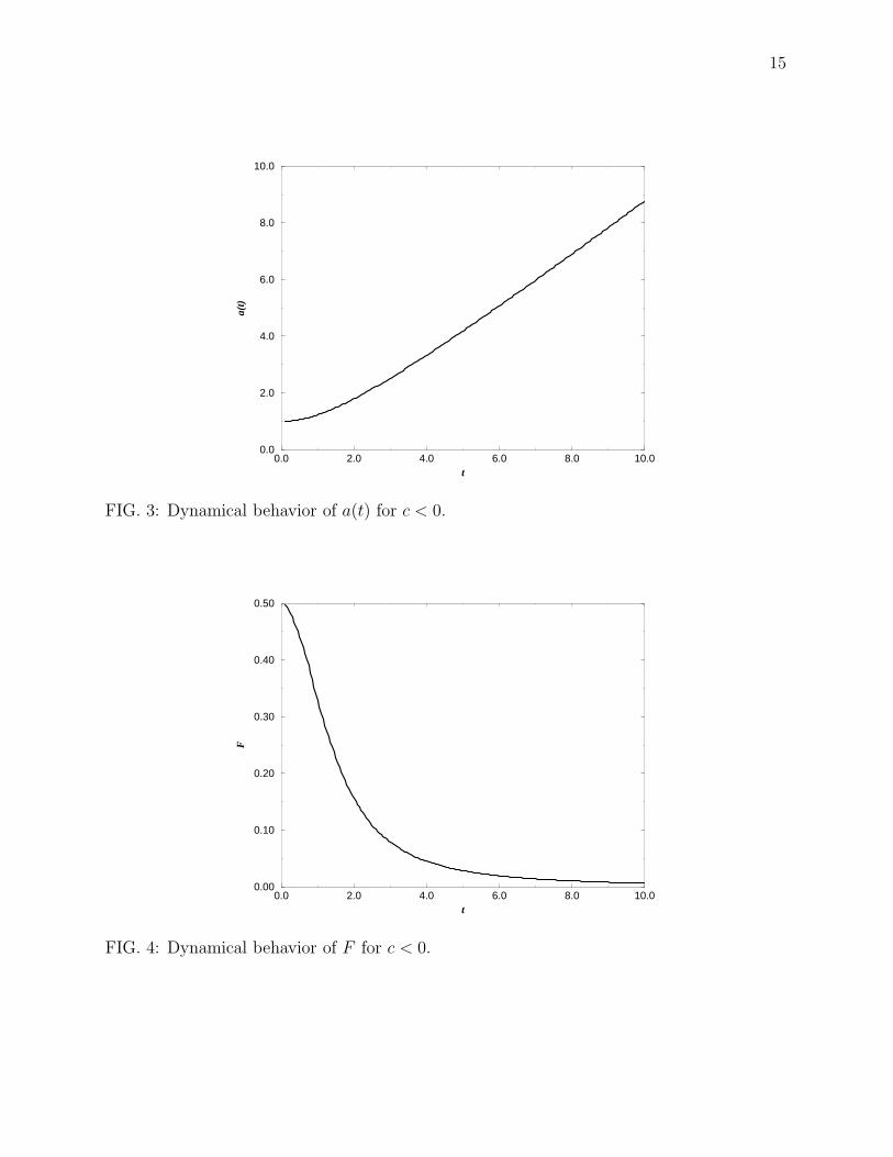
For those conditions we have a numerical solution for a(t) as shown in Fig. 3. For theCasimir force we have the behavior as shown in Fig. 4. For both cases the exact solutionhas very small oscillations, but overall is close to the Casimir solution, and is accuratelydescribed by the limits of that solution, Eqs. (4.26) and (4.24).

Thus, we have presented a formalism to describe the dynamical Casimir effect in theadiabatic approximation. It may be applied to an arbitrary GUT. Without any technicalproblems one can generalize the present consideration to any specific four-dimensional back-ground (we limited ourselves to a discussion of a toroidal FRW universe as providing themoving boundary conditions). But the limitations of our approach must be stressed: Itwould be extremely interesting to suggest new formulations of the dynamical Casimir effectbeyond the adiabatic approximation.

ACKNOWLEDGMENTS

We thank A. Bytsenko for helpful discussions. The work by SDO and KEO has beensupported in part by RFBR, that of SDO also by CONACyT, and that of KAM by the USDepartment of Energy.

APPENDIX A: ALTERNATIVE KINETIC ENERGY TERMS

In the text, we introduced an ad hoc kinetic energy term into the action, referring to thechange of scale with physical time,

∫

dt1

2ma2. (A1)

This is rather natural in the adiabatic context, where |a| � 1, for then simple scalingproperties obtain, as evidenced by the dimensional consistency of the resulting equationsof motion when m has dimensions of mass. But we can not offer very strong arguments in

12

its favor, in the absence of dynamical information. So, in this appendix we consider twoalternatives, which provide somewhat different models for the dynamical evolution of theworld.

In the first, we suppose that the same kinetic energy should be integrated over conformaltime,4

∫

dη1

2ma2 = m

∫

dt1

2

a2

a, (A2)

so that the Casimir evolution equation is, in place of Eq. (4.7),

1

2

ma2

a=

c

a+ k, (A3)

where we have dropped the subscript 0 for simplicity, and written the constant of integrationas k. The solution of this equation is very simple,

a = a0 + t

√

2

m

√

c + ka0 +k

2mt2, a0 = a(0). (A4)

If c > 0, we can set k = 0 and obtain instead of the behavior exhibited in Eq. (4.8), a lineargrowth of the scale,

a = a0 +

√

2c

mt. (A5)

If c < 0, as before we cannot set the integration constant equal to zero; if we again choosethe initial velocity to be zero, or a0 = −c/k, we get a result very like Eq. (4.26):

a = − c

k+

k

2mt2, (A6)

but now valid for all times.Perhaps a more natural possibility is to use the conformal time everywhere in the kinetic

energy term,5∫

dηm

2

(

da

dη

)2

=m

2

∫

dt a a2. (A7)

The solution to the purely Casimir dynamical equation is

m

2aa2 =

c

a+ k, (A8)

which is integrated to

t =1

k2

√

m

2

{

2

3

[

(ka + c)3/2 − (ka0 + c)3/2]

− 2c[

(ka + c)1/2 − (ka0 + c)1/2]

}

. (A9)

4In this case the parameter m is dimensionless.5In this case the parameter m has dimension 1/Length2.

13

When c > 0 again we can take k → 0, which leads to the k = 0 result

a2 = a20 + 2

√

2c

mt. (A10)

If c < 0 and we choose again ka0 + c = 0, we obtain for short times

a = − c

k+

k3

2mc2t2, t � 1, (A11)

again very similar to Eq. (4.26).In Figs. 5 and 6 we show the effect of the inclusion of the dynamical b term for these

kinetic energy structures. Qualitatively, the results do not depend much on whether theCasimir term is positive or negative. The example given for the first alternative kineticenergy is similar to the simple model result for c < 0 shown in Fig. 3 except that the growthin t is quadratic rather than linear. The evolution for the second form of kinetic energyresembles the simple model result for c > 0 shown in Fig. 1.

REFERENCES

[1] H. B. G. Casimir, Proc. K. Ned. Akad. Wet. 51, 793 (1948).[2] G. Plunien, B. Muller and W. Greiner, Phys. Reports 134, 87 (1986).[3] V. M. Mostepanenko and N. N. Trunov, The Casimir Effect and its Applications (Ox-

ford, London, 1997).[4] K. A. Milton, in Applied Field Theory, Proc. 17th Symposium on Theoretical Physics,

eds. C. Lee, H. Min and Q.-H. Park (Chungbum, Seoul, 1999), p. 1, hep-th/9901011.[5] S. K. Lamoreaux, Am. J. Phys. 67, 850 (1999).[6] G. T. Moore, J. Math. Phys. 11, 2679 (1970).[7] E. Sassaroli, Y. N. Srivastava and A. Widom, Phys. Rev. A 50, 1027 (1994).[8] V. V. Dodonov, A. B. Klimov and V. I. Man’ko, Phys. Lett. A 142, 511 (1989); R.

Golestanian and M. Kardar, Phys. Rev. A 58, 1713 (1998).[9] Y. Nagatani and K. Shigetomi, hep-th/9904193.

[10] I. L. Buchbinder, S. D. Odintsov and I. L. Shapiro, Effective Action in Quantum Gravity,IOP Publishing, Bristol and Philadelphia, 1992.

[11] R. Reigert, Phys. Lett. B 134, 56 (1984); E. S. Fradkin and A. A. Tseytlin, Phys. Lett.B 134, 187 (1984); I. L. Buchbinder, S. D. Odintsov, and I. L. Shapiro, Phys. Lett. B

162, 92 (1985).[12] I. Brevik and S. D. Odintsov, Phys. Lett. B 455, 104 (1999); hep-th/9902184.[13] E. Elizalde, S.D. Odintsov, A. Romeo, A.A. Bytsenko and S. Zerbini, Zeta Regulariza-

tion With Applications (World Scientific, Singapore, 1994).[14] I. J. Zucker, J. Phys. A: Math. Gen. 8, 1734 (1975).[15] I. Brevik, V. N. Marachevsky, and K. A. Milton, Phys. Rev. Lett. 82, 3948 (1999).[16] G. Barton, J. Phys. A: Math. Gen. 32, 525 (1999).[17] M. Bordag, K. Kirsten, and D. Vassilevich, Phys. Rev. D 59, 085011 (1999).[18] J. S. Høye and I. Brevik, quant-ph/9903086; to appear in the Stell issue of J. Statistical

Phys.

14

FIGURES

0.0 2.0 4.0 6.0 8.0 10.0t

0.0

5.0

10.0

a(t)

FIG. 1: Casimir (dashed line) and dynamical behavior for a(t) for c > 0.

0.0 2.0 4.0 6.0 8.0 10.0t

-1.0

-0.5

0.0

F

FIG. 2: Casimir (dashed line) and dynamical behavior of F for c > 0.

15

0.0 2.0 4.0 6.0 8.0 10.0t

0.0

2.0

4.0

6.0

8.0

10.0

a(t)

FIG. 3: Dynamical behavior of a(t) for c < 0.

0.0 2.0 4.0 6.0 8.0 10.0t

0.00

0.10

0.20

0.30

0.40

0.50

F

FIG. 4: Dynamical behavior of F for c < 0.

16

0.0 2.0 4.0 6.0 8.0 10.0t

0.0

20.0

40.0

60.0

80.0

100.0

a(t)

FIG. 5: Dynamical behavior for a(t) for the first alternative kinetic energy term, Eq. (A2).Shown are the behaviors with m = 1, and initial condition a(0) = 1, evolving initially untilt = 0.01 according to Eq. (A4), with c = 1, k = 1 (solid line); and with c = −1, k = 2(dashed line).

0.0 2.0 4.0 6.0 8.0 10.0t

0.0

2.0

4.0

6.0

8.0

a(t)

FIG. 6: Dynamical behavior for a(t) for the second alternative kinetic energy term, Eq. (A7).Shown are the behaviors with m = 1, and initial condition a(0) = 1, evolving initially untilt = 0.01 according to Eq. (A9), with c = 1, k = 1 (solid line); and with c = −1, k = 2(dashed line).