DYNAMIC TRAFFIC ASSIGNMENT: PROPERTIES AND ...

Transportmetrica, Vol. 2, No. 1 (2006), 31-52

31

DYNAMIC TRAFFIC ASSIGNMENT: PROPERTIES AND EXTENSIONS

W.Y. SZETO1 AND HONG K. LO2

Received 18 March 2005; received in revised form 9 September 2005; accepted 30 September 2005 Dynamic Traffic Assignment (DTA) is long recognized as a key component for network planning and

transport policy evaluations as well as for real-time traffic operation and management. How traffic is encapsulated in a DTA model has important implications on the accuracy and fidelity of the model results. This study compares and contrasts the properties of DTA modelled with point queues versus those with physical queues, and discusses their implications. One important finding is that with the more accurate physical queue paradigm, under certain congested conditions, solutions for the commonly adopted dynamic user optimal (DUO) route choice principle just do not exist. To provide some initial thinking to accommodate this finding, this study introduces the tolerance-based DUO principle. This paper also discusses its solution existence and uniqueness, develops a solution heuristic, and demonstrates its properties through numerical examples. Finally, we conclude by presenting some prospective future research directions.

KEYWORDS: Dynamic traffic assignment, point queue, physical queue, bounded rationality, cell transmission

model, route swapping algorithm

1. INTRODUCTION The properties of dynamic traffic assignment (DTA) have important implications on its

ability to portray the actual travel behaviour, and hence on the fidelity and accuracy of the model results. These properties depend strongly on the two components of DTA: the travel choice principle and the traffic-flow component. The travel choice principle models travellers’ propensity to travel, and if so, how they select their routes, departure times, modes, or destinations. In making such choices, travel time is one important element of their considerations. The commonly adopted travel choice principle is the dynamic extension of Wardrop’s (1952) principle called the Dynamic User Optimal (DUO) principle or its stochastic extension, Stochastic Dynamic User Optimal (SDUO) (Ran and Boyce, 1996). The travel choice principle can be formulated as either a nonlinear complementarity problem, variational inequality problem, or fixed-point problem. It is established that the existence of solutions requires the mapping function of the problem to be continuous (Theorem 1.4 in Nagurney, 1993) whereas the uniqueness of solution further requires the mapping function to be strictly monotonic (Theorem 1.8 in Nagurney, 1993). Therefore, solution existence (uniqueness) requires route travel times to be continuous (strictly monotone) with respect to route flows.

The traffic-flow component depicts how traffic propagates on a transport network and hence governs the network performance in terms of travel time. This component can be modelled as a set of side constraints, as is traditionally accomplished. However, this approach could be cumbersome, rendering the resultant formulation hard to solve (Lo and Szeto, 2002a). Modelling the traffic-flow component as a unique mapping of route flows, on the other hand, opens up a new way to analyze DTA problems (e.g., Lo and Szeto, 2002a,b, 2004, 2005; Szeto and Lo, 2004), with the outputs of this mapping being the route travel times. This approach has two advantages: namely, first, it ensures the consistency between link travel times and link exit flows because link travel times are 1 Department of Civil, Structural, and Environmental Engineering, Trinity College, University of Dublin, Dublin 2, Ireland. Corresponding author (E-mail: [email protected]). 2 Department of Civil Engineering, The Hong Kong University of Science and Technology, Clear Water Bay, Hong Kong SAR, P.R. China.

32

uniquely derived from exit link flows; second, it allows us to determine the existence and uniqueness of solutions of DTA problems directly by simply checking whether the unique mapping is continuous and strictly monotonic.

Capturing actual traffic behaviour in the traffic-flow component is one important current research direction. Indeed, past efforts have focused on capturing the following traffic behaviour: 1) First-in first-out (FIFO) (e.g., Jayakrishnan et al., 1995; Astarita, 1996; Heydecker

and Addison, 1998; Tong and Wong, 2000; Huang and Lam, 2002; Carey et al., 2003; Szeto and Lo, 2004): FIFO on the link level means that users who enter the link earlier will leave it sooner;

2) Causality (e.g., Friesz et al., 1993; Heydecker and Addison, 1998; Carey et al., 2003): Causality means that the speed and travel time of a vehicle on a link is only affected by the speed of vehicles ahead, and;

3) Queue spillback (e.g., Daganzo, 1994, 1995; Lo, 1999; Adamo et al., 1999; Tong and Wong, 2000; Kuwahara and Akamatsu, 2001; Rubio-Ardanaz et al., 2001, Lo and Szeto, 2002a,b, 2004, 2005; Szeto and Lo, 2004; Ziliaskopoulos et al., 2004): Queue spillback refers to the end of queue spilling backwards in the network.

The above traffic behaviour governs the properties of DTA formulations such as the properties of route and origin-destination (OD) costs (e.g., continuity of route and OD costs), as well as solution properties (e.g., existence of solutions). The thesis “DTA: formulations, properties and extensions” (Szeto, 2003) studies and compares the properties of DTA with point queues and those with physical queues. One major finding in Szeto (2003) is that capturing detailed traffic dynamics, such as queue spillback, may violate the requirement on solution existence, resulting in the non-existence of DUO solutions. This finding shakes the very foundation of the analytical DTA approach. To accommodate this result, Szeto (2003) proposes the tolerance-based DUO principle, adapted from the bounded rationality notion originally proposed by Simon (1955). The notion of bounded rationality is also used by Mahmassani and colleagues (e.g., Mahmassani and Chang, 1987; Jayakrishnan et al., 1994; Hu and Mahmassani, 1997; Mahmassani and Liu, 1999) to capture the behaviour of individual travellers. The tolerance-based DUO principle here, however, is used to describe the route choice principle at the system level, as consistent with analytical DTA approaches, so that its properties in terms of solution existence and uniqueness can be explored. It can be considered as a relaxation of the traditional DUO principle with the traditional DUO principle as a special case.

In this study, we illustrate, via a numerical example, how the point queue and physical queue paradigms can produce very different queuing predictions in congested networks wherein junction blockage is common. In the second example, we demonstrate the effect of parameters in the proposed heuristic route-swapping algorithm on the existence of solutions. In the third numerical example, we show how, in the absence of a traditional DUO solution, the tolerance-based DUO principle performs. The rest of paper is organized as follows. The next section discusses the properties of DTA with or without physical queue consideration, and their implications. Section 3 depicts the proposed tolerance-based DUO principle. Section 4 formulates the tolerance-based DUO route choice problem and discusses the existence and uniqueness of solutions. The route-swapping heuristic and numerical examples are then described in Sections 5 and 6, respectively. Finally, Section 7 gives the summary and possible future research directions.

33

2. PROPERTIES OF DTA AND THEIR IMPLICATIONS Due to the space limitation, this section only summarizes the properties of DTA under

the point-queue (e.g., Yang and Meng, 1998; Huang and Lam, 2002) and physical-queue (e.g., Tong and Wong, 2000; Lo and Szeto, 2002a, b, 2004, 2005) representations analyzed in Szeto (2003), including the route and OD travel costs as well as the solution properties of DTA, and discusses their implications. The properties are summarized in Table 1.

TABLE 1: A comparison of the properties between point-queue and physical-queue

DTA problems (a) Properties of route costs

Route cost properties Point-queue problems Physical-queue problems Continuity w.r.t. route flows Continuous under mild assumptions Possibly discontinuous

Monotonicity w.r.t. route flows Usually non-monotonic Usually non-monotonic

Differentiability w.r.t. route flows Differentiable under differentiable link travel time functions and

non-differentiable under continuous exit flow functions

Possibly non-differentiable

Continuity of OD travel time w.r.t.demands

Continuous under mild assumptions Possibly discontinuous

(b) Solution properties Solution properties Point-queue problems Physical-queue problems

Causality Obey causality for all existing link travel time functions but do not

follow causality for some exit flow functions; e.g. exit flow at a

particular time is a function of the number of vehicles at that time

Obey causality

Link FIFO May or may not satisfy Link FIFO, depending on the choice of travel

time or exit flow functions

May or may not satisfy Link FIFO, depending on whether

additional variables are introduced to capture Link

FIFO

Route FIFO Satisfy Route FIFO if they satisfy Link FIFO

Satisfy Route FIFO if they satisfy Link FIFO

OD FIFO Satisfy this property under the DUO condition and certain assumptions,

but not satisfy under the SDUO conditions

Satisfy this property under the DUO condition and certain assumptions, but not satisfy under the SDUO conditions

Existence Must exist May not exist

Uniqueness Non-unique in terms of route flows and link flows

Non-unique in terms of route flows and link flows

2.1 Common properties and their implications

Under both queuing representations, we observe that

(i) The route cost is non-monotonic with respect to route flows; (ii) The route cost is non-differentiable with respect to route flows if certain traffic

flow models are adopted;

34

(iii) Whether the solutions follow causality and FIFO (on the link, route and origin destination (OD) level) depends on the underlying traffic flow models employed, and;

(iv) Solutions may not be unique if they exist. The non-monotone and non-differentiability properties lead to difficulties in finding

solutions if one exists at all, because the convergence of existing algorithms rely on either monotonicity or differentiability. One may rely on less restrictive algorithms such as genetic algorithm (e.g., Lo and Szeto, 2002b) or simulated annealing (e.g., Friesz et al., 1992) for solutions.

Violations of Link FIFO and causality imply poor reflection of reality because traffic tends to behave in a FIFO manner (Carey, 1992) and that vehicle following is consistent with causality (Heydecker and Addison, 1998). Models that exhibit these violations are unreliable.

The non-uniqueness of link flows implies that traffic can be predicted differently in various solutions. This raises the question of accuracy of the DTA models for various applications. Other than this, in actual applications, one must consider all possible solutions to cater for the worse-case scenarios in the planning and design. 2.2 Unique properties of physical-queue DTA and their implications

According to Table 1, we can observe three unique properties for the physical-queue

DTA as compared with the point queue one, which are summarized in the following propositions:

Proposition 1: Under the physical queue representation, route costs may not be continuous with respect to route flows.

Proposition 2: Under the physical queue representation, OD travel costs may not be continuous with respect to demands.

Proposition 3: A Wardropian solution may not exist to the DTA problem with physical queues.

All these unique properties are related to the existence of solutions to DTA problems. The implication of the discontinuity property of the supply function (proposition 2) is that solutions may not exist for DUO problems with elastic demands. For any OD pair at any departure time, one can imagine that three situations can happen as shown in Figure 1. For cases (i) and (iii), a solution exists to the problem but for case (ii), no solution exists! For the fixed demand case, as demonstrated in Szeto (2003), and summarized in Table 1 and proposition 3, we clearly observe the trade-off between the existence of solutions and the levels of traffic dynamics captured; point-queue DTA solutions always exist whereas those for physical-queue problems may not. The reason is that under congested conditions, the route travel time functions may become discontinuous (proposition 1), making it impossible in certain cases to find solutions that satisfy the equilibrium route choice principle perfectly. If the objective is to achieve DUO solutions, then DTA models with physical queues may be a problem despite that they can model the actual traffic flow features better. This theoretical finding may prove to be important in the search of new behaviour rules for analytical formulations that are behaviourally sound and consistent with the actual network behaviour. Sections 3 to 5 describe the work in Szeto (2003) in dealing with the possibility of the non-existence of solutions to the DTA problems with physical queues.

35

FIGURE 1: Three possible scenarios for the DUO problem with elastic demands

3. TOLERANCE-BASED DYNAMIC USER OPTIMAL PRINCIPLE The tolerance-based DUO principle proposed by Szeto (2003) requires the travel times

of all used routes between the same OD pair to be similar, or within an acceptable tolerance maxε from the minimum OD route travel time, where the tolerance level is purely a function of the behaviour of the network users. This principle, adapted from the bounded-rationality behavioural notion, can be expressed as: If 0)( >tf rs

p , then max)()( ε≤π−η tt rsrsp , (1)

tprstt rsrsp ,,,0)()( ∀≥π−η , (2)

where )(tf rsp and )(trs

pη are respectively the flow between OD pair rs entering route p

at time t and the corresponding route travel time; )(trsπ is the shortest OD travel time

between OD pair rs for flows departing at time t; maxε is the acceptable tolerance, a non-negative parameter obtained through travel behaviour surveys and experiments. In (1)-(2), t is an instant of time; in this paper, t is a time-slice index, as we consider a discrete-time DTA formulation. Condition (2) is included in this principle to ensure

)(trsπ to be the shortest OD travel time among all the possible routes between OD pair

rs for flows departing at time t. By employing the following transformation function:

⎩⎨⎧

>≤≤=ε uyy

uyuy if0fi0),( , (3)

where u and y are independent non-negative variables, the tolerance-based DUO principle can be alternatively formulated as: ( ) tprstttf rsrs

prsp ,,,0),()()( max ∀=επ−ηε⋅ , (4)

( ) tprstt rsrsp ,,,0),()( max ∀≥επ−ηε . (5)

Condition (5) implies condition (2) due to the requirement of the non-negative independent variable for the transformation function. Condition (4) implies (1), meaning that the travel time of a used route is greater than the minimum route travel time by not more than an acceptable level maxε . According to (4), if route p carries a positive flow

Case (i)

Case (ii)

Case (iii)

OD demand

OD travel time

Demand function

36

at time t (i.e., 0)( >tf rsp ), the transformation function ( )max),()( επ−ηε tt rsrs

p must be

equal to zero, implying max)()(0 ε≤π−η≤ tt rsrsp due to the first condition of (3). In

other words, if route p carries a positive flow at time t, the travel time of route p is greater than the minimum route travel time by not more than an acceptable level maxε .

Note that if route p carries zero flow at time t (i.e., 0)( =tf rsp ), ( )max),()( επ−ηε tt rsrs

p

must be nonnegative due to (5) and hence the route travel time )(trspη must be greater

than or equal to the minimum route travel time )(trsπ .

As a special case, if maxε equals zero, conditions (4)-(5) can be reduced to the following: ( ) tprstttf rsrs

prsp ,,,00),()()( ∀=π−ηε⋅ , (6)

( ) tprstt rsrsp ,,,00),()( ∀≥π−ηε . (7)

According to (3), we have:

)()(0)()(if)()(

0)()(0if0)0),()(( tt

tttt

tttt rsrs

prsrsp

rsrsp

rsrsprsrs

p π−η=⎪⎩

⎪⎨⎧

>π−ηπ−η

≤π−η≤=π−ηε .

Therefore, equations (6)-(7) can be simplified to: ( ) tprstttf rsrs

prsp ,,,0)()()( ∀=π−η , (8)

tprstt rsrsp ,,,0)()( ∀≥π−η , (9)

or If 0)( >tf rs

p , then 0)()( =π−η tt rsrsp , (10)

tprstt rsrsp ,,,0)()( ∀≥π−η . (11)

Conditions (8)-(9) are the ideal DUO conditions. That is, if maxε equals zero, equations (4)-(5) can be reduced to the ideal DUO conditions. According to this result, the tolerance-based principle is a generalization of the traditional DUO principle.

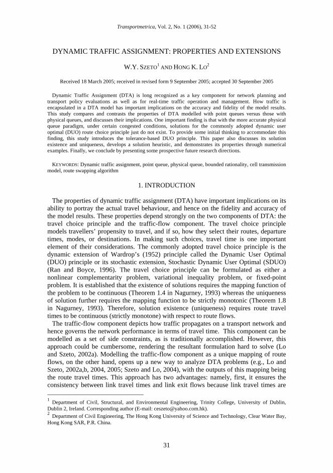
4. TOLERANCE-BASED DUO ROUTE CHOICE PROBLEM

4.1 Nonlinear complementarity problem (NCP) formulation

For fixed demands, the DTA problem with the tolerance-based DUO route choice

principle is to find a route flow vector *f such that: ( ) tprstttf rsrs

prsp ,,,0),()()( max ∀=επ−ηε⋅ , (12)

( ) tprstt rsrsp ,,,0),()( max ∀≥επ−ηε , (13)

trstqtf rsp

rsp ,),()( ∀=∑ , (14)

tprst rstp

rsp ,,),()( , ∀Φ=η f , (15)

37

0≥f , (16) where )(tqrs is the demand of OD pair rs at time t; (.),

rstpΦ is a unique mapping

yielding route travel times for a given route flow vector f . Equations (12)-(13) express the tolerance-based DUO principle. Equations (14) and

(16) are the flow conservation and non-negativity conditions. Equation (15) considers the traffic flow component as a unique functional mapping yielding route travel times for given route flows. Many traffic flow models can be used for this mapping. Szeto’s (2003) numerical studies adopt the Cell Transmission Model (CTM) (Daganzo, 1994, 1995) as the underlying traffic flow model to capture the effect of realistic physical queuing, such as queue formation and dissipation, and queue spillback. In determining the route travel times in (15), we first use CTM to simulate the resultant traffic pattern, followed by the route travel time extraction procedure developed in Lo and Szeto (2002a). As CTM uses mathematical operations that produce unique traffic patterns for given route flows, and the route travel time extraction procedure produces unique outputs for given cumulative inflow and outflow curves, we establish a unique mapping yielding route travel costs for given route flows. The details of encapsulating CTM for dynamic traffic assignment models can be found in Lo (1999) and Lo and Szeto (2002a, b).

The tolerance-based DUO route choice problem (12)-(16) can be reformulated as an NCP by introducing three more conditions. By attaching )(trsπ to the flow conservation

condition (14), we obtain:

trstqtft rsp

rsp

rs ,,0)()()( ∀=⎟⎠⎞⎜

⎝⎛ −π ∑ . (17)

As ),(trsπ the shortest OD travel time, must be greater than zero,

0)()( =−∑ tqtf rsp

rsp must hold at optimality. Adding this to the problem (12)-(16)

will not alter the optimality condition. For mathematical completeness, we also introduce two more conditions to the original problem: trstrs ,,0)( ∀≥π , (18)

trstqtf rsp

rsp ,,0)()( ∀≥−∑ . (19)

They include 0)( >π trs and 0)()( =−∑ tqtf rsp

rsp as special cases and therefore do

not change the optimality condition of the original problem (12)-(16). The DUO route choice problem with fixed demands can then be considered as the problem of finding a route flow vector *f to satisfy (12)-(19).

By putting (15) into (12) and (13), the DUO route choice problem with fixed demands (12)-(19) can be written as an NCP: to find *x such that:

0≥⎟⎠⎞⎜

⎝⎛= π

fx , (20)

( )( ) 0, **T* =Φ⋅ fxFx , (21) and ( )( ) 0, ** ≥Φ fxF , (22) where

38

⎟⎟

⎠

⎞

⎜⎜

⎝

⎛

∀π

∀=

trst

tprstfrs

rsp

,),(

,,),(x , (23)

( )( )( )( )

⎟⎟⎟

⎠

⎞

⎜⎜⎜

⎝

⎛

∀−

∀επ−Φε=Φ

∑ trstqtf

tprstrs

prsp

rsrstp

,),()(

,,,),(,

max, ffxF , (24)

and ( )fΦ is a vector of ( )( )tprsrstp ,,,, ∀Φ f ; π is a vector of shortest OD travel times, and;

)(tf rsp , )(trs

pη , )(trsπ , maxε , )(tqrs , and ( ).,rs

tpΦ follow earlier definitions.

4.2 Solution existence and uniqueness

For ease of explanation, we first define a non-negative gap function ( )fH :

( ) ( )( )tprstttH rsrsp

rsp ,,,)()()(max ∀π−η⋅δ=f , (25)

where the indicator variable )(trspδ equals 1 if the flow on route p between OD pair rs at

time t is nonzero, and equals zero otherwise. This gap is the largest difference between the travel times of all used routes and the corresponding shortest OD travel times under the route flow pattern f, and measures how far the current solution is from the traditional DUO solution.

To analyze the existence and uniqueness of solutions, we define the theoretical gap (TG), which is the minimum of the largest difference between the travel times of all used routes and the corresponding shortest OD travel times of all feasible flow patterns. In other words, TG is the smallest gap of all the feasible solutions. Mathematically, the theoretical gap (TG) is expressed as follows: ( ) 0minTG ≥= f

fH , (26)

The value of the theoretical gap depends on the network and the demand pattern. In DTA formulations with the more realistic physical-queue representation, the route

travel time functions are not always continuous with respect to the route flows, rendering the existence of solutions not always possible (propositions 1 and 3), or equivalently their theoretical gap never reaches zero. For the tolerance-based DUO route choice problem with physical queues, in a similar manner, solution existence is not guaranteed. A solution exists to the problem if and only if the theoretical gap is less than or equal to

maxε : ( ) maxminTG ε≤= f

fH . (27)

According to (27), the existence of solutions to the physical-queue tolerance-based DUO problem depends on the theoretical gap (which is related to the network topology and demand pattern) and the parameter maxε (which is related to the behaviour of the network users). In general, as maxε and hence the constraint (27) are gradually relaxed, solution existence gradually becomes easier. However, we emphasize the importance of specifying the tolerance level from a behaviour perspective rather than as a numerical means for obtaining equilibrium solutions. If the tolerance level is specified at a level higher than the actual behaviour, then the solution will stop at a premature “equilibrium”, even though in reality, travellers are still swapping routes in the search of better ones. In

39

summary, solution existence is both a function of the network topology and travel demand, and the behavioural tolerance of the users on route swapping.

On the issue of uniqueness of solution, as one can see, when maxε approaches infinity, all feasible gap values satisfy (27) and hence the corresponding flows are solutions, implying that multiple solutions are possible in this problem. In fact, even if the tolerance is zero (i.e., the problem becomes the traditional DUO problem), multiple solutions can still be possible as discussed in Section 2.1.

5. SOLUTION METHOD

This paper adopts the heuristic day-to-day route-swapping algorithm developed in

Szeto (2003), which is modified from the route-swapping algorithm in Huang and Lam (2002). The advantage of this algorithm is that no matter the tolerance-based or traditional DUO solutions exist or not, the algorithm can simulate day-to-day flow patterns in addition to the within-day flow patterns. That is, the transition from disequilibrium to equilibrium or one state of disequilibrium to another can be described. This allows us to study the daily variations in network performance. The algorithmic detailed steps are outlined as follows: Step 1: Set the iteration counter τ = 1. Choose the initial route flow τ)(tf rs

p .

Step 2: Determine the route travel time τη )(trsp through CTM and the route travel time

extraction procedure as described in Lo (1999) and Lo and Szeto (2002a,b). Find ( )ptt rs

prs ∀η=π ττ ,)(min)( .

Step 3: Update the route flow as below: ( )( )ττττ+τ π−ηρ−= )()()()(,0max)( 1 tttftftf rsrs

prsp

rsp

rsp , rs

trs PPp τ∈ ,/ ,

rst

rsrsp

rsp

P

ttftf

τ

ττ+τ

ψ+=

,1

)()()( , rs

tPp τ∈ , ,

where ( )∑

τ∈+τττ −=ψ

rst

rs PPp

rsp

rsp

rs tftft,/

1)()()( ;

{ }max, )()(:max ε≤π−η= τττ ttpP rsrsp

rst ;

rsP is the set of all feasible paths between OD pair rs.

Step 4: Stop if ( ) maxε≤τfH or maxτ=τ , where

( ) ( )( )tprstttH rsrsp

rsp ,,,)()()(max ∀π−η⋅δ= ττττf and maxτ is the maximum

number of iterations; Otherwise, set 1+τ=τ and return to Step 2.

6. NUMERICAL STUDIES

In the three numerical studies conducted in this section, we aim to illustrate i) the difference between the point-queue and physical-queue modelling paradigms in terms of predicting queuing locations over time, the link occupancies over time, travel times, and

40

the resultant route choice pattern, ii) the effects of the tolerance and swapping rate on the existence of solutions, and iii) the impact of the initial solution and swapping rate on the final solution as well as on the non-equilibrium traffic pattern. The scenario setup for the last two numerical studies adopts from that in Szeto (2003) wherein the traditional DUO solution is known not to exist. 6.1 A comparison between point queue and physical queue paradigms

The scenario network consists of five nodes, four links and two OD pairs as shown in

Figure 2. The two OD pairs are from node 1 to node 4 and from node 1 to node 5. Each OD pair contains one route. The route between OD pair (1,4) is called Route 1 whereas the route between OD pair (1,5) is called Route 2. The modelling horizon is set at 1200 seconds. Traffic demand from node 1 to node 4 is 5400 vph and lasts for 200 seconds from the start of the modelling horizon. Traffic demand from node 1 to node 5 between time ω = 201 seconds and time ω = 300 seconds is 3600 vph. The detailed input parameters include: a. Free flow travel speed and shockwave speed: 48 km/hour b. Length of each link: Links (1,2) and (2,5): 1.067 km; Link (2,3): 0.4 km; Link (3,4):

0.667 km c. Number of lanes: Links (1,2), (2,3), and (2,5): 3; Link (3,4): 1 d. Saturation flow rate: 1800 vehicles/hour/lane e. Jam density: 125 vehicles/km f. The length of each time interval: 10 seconds

1

2

5

3

Origin

Destination4 Destination

FIGURE 2: The scenario network for Example 6.1

The results obtained from the cell transmission model (CTM) are compared with those

from the simplified cell transmission model (SCTM), which ignore the storage capacity term in CTM. Conceptually, SCTM is similar to the one proposed by Smith (1993). This type of point queue models, including SCTM and Smith’s model, is seldom proposed in the literature as a link is required to be divided into many segments which causes computational inefficiency when compared with other point-queue models. SCTM is adopted here to clearly show the traffic over time and space. If other point-queue models are used, a linear interpolation is required to obtain the occupancy over time and space.

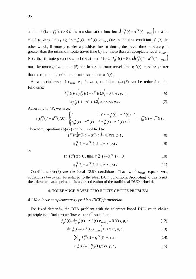
Figure 3 and Figure 4 show the occupancy plots over time and space under the two modelling paradigms. The intensities of the shades correspond to the occupancy levels, as shown in the legend on the right side of the plot. As is customary, traffic propagates in

41

(a) Point-queue paradigm

Time (seconds) Node 1

Node 4

Node 2

Node 3

0 200 400 600 800

120

(b) Physical-queue paradigm

Time (seconds) Node 1

Node 4

Node 2

Node 3

200 3000 200 400 600 800

FIGURE 3: Occupancy plots along Route 1

42

(a) Point-queue paradigm

Time (seconds) Node 1

Node 5

Node 2

280

0 200 400 600 800

(b) Physical-queue paradigm

Time (seconds) Node 1

Node 5

Node 2

0 200 400 600 800 440

FIGURE 4: Occupancy plots along Route 2

43

100

150

200

250

300

350

210 230 250 270 290Departure time (seconds)

Rou

te tr

avel

tim

e(s

econ

ds)

point queuephysical queue

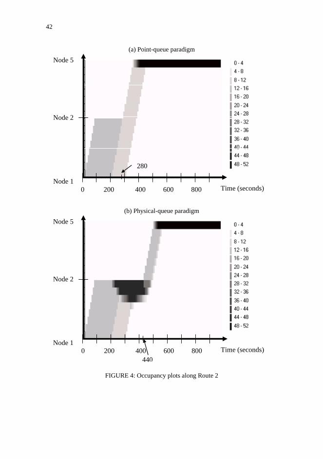
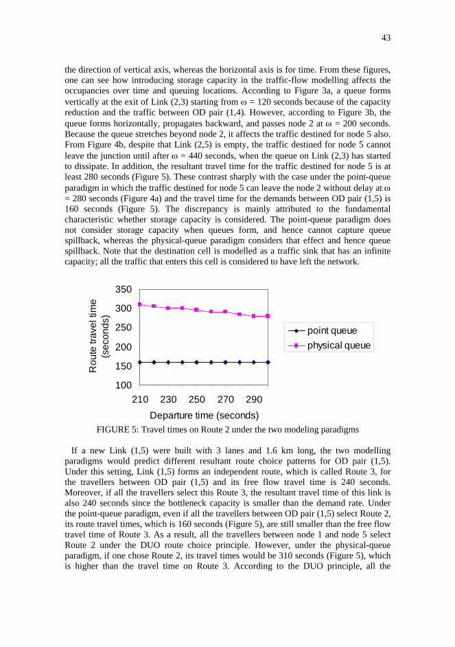
the direction of vertical axis, whereas the horizontal axis is for time. From these figures, one can see how introducing storage capacity in the traffic-flow modelling affects the occupancies over time and queuing locations. According to Figure 3a, a queue forms vertically at the exit of Link (2,3) starting from ω = 120 seconds because of the capacity reduction and the traffic between OD pair (1,4). However, according to Figure 3b, the queue forms horizontally, propagates backward, and passes node 2 at ω = 200 seconds. Because the queue stretches beyond node 2, it affects the traffic destined for node 5 also. From Figure 4b, despite that Link (2,5) is empty, the traffic destined for node 5 cannot leave the junction until after ω = 440 seconds, when the queue on Link (2,3) has started to dissipate. In addition, the resultant travel time for the traffic destined for node 5 is at least 280 seconds (Figure 5). These contrast sharply with the case under the point-queue paradigm in which the traffic destined for node 5 can leave the node 2 without delay at ω = 280 seconds (Figure 4a) and the travel time for the demands between OD pair (1,5) is 160 seconds (Figure 5). The discrepancy is mainly attributed to the fundamental characteristic whether storage capacity is considered. The point-queue paradigm does not consider storage capacity when queues form, and hence cannot capture queue spillback, whereas the physical-queue paradigm considers that effect and hence queue spillback. Note that the destination cell is modelled as a traffic sink that has an infinite capacity; all the traffic that enters this cell is considered to have left the network.

FIGURE 5: Travel times on Route 2 under the two modeling paradigms If a new Link (1,5) were built with 3 lanes and 1.6 km long, the two modelling

paradigms would predict different resultant route choice patterns for OD pair (1,5). Under this setting, Link (1,5) forms an independent route, which is called Route 3, for the travellers between OD pair (1,5) and its free flow travel time is 240 seconds. Moreover, if all the travellers select this Route 3, the resultant travel time of this link is also 240 seconds since the bottleneck capacity is smaller than the demand rate. Under the point-queue paradigm, even if all the travellers between OD pair (1,5) select Route 2, its route travel times, which is 160 seconds (Figure 5), are still smaller than the free flow travel time of Route 3. As a result, all the travellers between node 1 and node 5 select Route 2 under the DUO route choice principle. However, under the physical-queue paradigm, if one chose Route 2, its travel times would be 310 seconds (Figure 5), which is higher than the travel time on Route 3. According to the DUO principle, all the

44

Origin Destination

(20,5)

(30,5)

8

(30,15)

5

Destination

(10,5)2 3 4

9

7

Origin(10,5)

(30,5)(10,5)

(50,20)

(40,20)(50,5)

10(10,5)

1 6(145,5)

Key:

travellers between OD pair (1,5) choose Route 3. This observation agrees with the results shown in Kuwahara and Akamatsu (2001).

This numerical example clearly shows that the predictions about queuing locations over time, the link occupancies over time, travel times, and the route choice pattern from physical-queue models are substantially different from those from point-queue ones in congested networks wherein junction blockage is common. The discrepancy is mainly attributed to the fundamental characteristic whether storage capacity is considered, and causes the network designs and traffic management schemes based on the point-queue models to be totally different from those based on physical-queue models. This seems to indicate that 1) simplifications from the physical-queue representation are inadequate in producing correct estimation results, and 2) resources for improving the current situation may be wrongly allocated if we rely on the estimation from point-queue models. 6.2 Sensitivity of swapping rate and tolerance

In this second numerical study, we illustrate how the tolerance-based DUO formulation

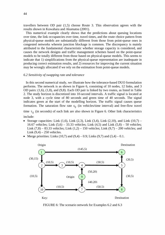
performs. The network is as shown in Figure 6, consisting of 10 nodes, 12 links, and 3 OD pairs: (1,6), (1,8), and (9,8). Each OD pair is linked by two routes, as listed in Table 2. The study horizon is discretized into 10-second intervals. A traffic signal is located at node 3, with a cycle time of 80 seconds and green time of 40 seconds. The signal indicates green at the start of the modelling horizon. The traffic signal causes queue formation. The saturation flow rate ijs (in vehicles/time interval) and free-flow travel

time ijτ (in seconds) of each link are also shown in Figure 6. Other link characteristics include: • Storage capacities: Link (1,6), Link (2,3), Link (3,4), Link (2,10), and Link (10,7) –

16.67 vehicles; Link (5,6) – 33.33 vehicles; Link (4,5) and Link (5,8) – 50 vehicles; Link (7,8) – 83.33 vehicles; Link (1,2) – 150 vehicles; Link (9,7) – 200 vehicles; and Link (9,4) – 250 vehicles.

• Merge priorities: Links (10,7) and (9,4) – 0.9; Links (9,7) and (3,4) – 0.1.

FIGURE 6: The scenario network for Examples 6.2 and 6.3

45

TABLE 2: OD – Route characteristics OD pair Route number Node sequence Free-flow travel time (seconds)

1 1-2-3-4-5-6 100 (1, 6) 6 1-6 145 2 1-2-3-4-5-8 110 (1, 8) 3 1-2-10-7-8 100 4 9-7-8 90 (9, 8) 5 9-4-5-8 110

The departure time of traffic leaving an origin is indexed by t. Given that time is

discretized at 10-second intervals, the actual departure time is thus 10t. In this example, we fix the route flows at the various departure times as:

⎩⎨⎧

>== 40

3,2,15)(161 t

ttf ; ⎩⎨⎧ == otherwise0

6,55)(8163

ttf ; ⎪⎩

⎪⎨⎧

==

=otherwise0

98811

)(8984 t

ttf ;

ttftftf ∀=== ,0)()()( 166

985

182 .

For each combination of swapping rate and tolerance, the route-swapping algorithm is employed to determine solutions. The initial solution is obtained by an all-or-nothing assignment procedure. The algorithm stops when a tolerance-based DUO solution is found or when the maximum iteration number of 2000 is reached. The number of iterations performed for each combination of swapping rate and tolerance is shown in Table 3. An entry of “2000” indicates that the maximum number of iterations is reached without finding an equilibrium solution. This table clearly shows that the tolerance maxε and swapping rate ρ are important variables for reaching the tolerance-based DUO solutions (if they are reachable at all). The reason is that, as explained before, to a great extent, the tolerance defines the requirement of obtaining solutions. A higher tolerance means a lower requirement. Moreover, higher swapping rates or larger step sizes often cause the algorithm to hop from one point to another without approaching to the solution location. In this particular example, the shaded region in Table 3 represents the region wherein the route-swapping algorithm finds a solution. Obviously, this result is case-specific and network-dependent, but generally one can see that a smaller swapping rate and a higher tolerance are generally more capable of stopping at an equilibrium solution.

The swapping rate not only has implications on the possibility of finding solutions, but also on the computational time required for finding solutions, as one may expect. For a fixed tolerance, if the solution is reachable, higher swapping rates typically mean faster solution times by having to go through a smaller number of iterations. For example, in Table 3, for the same maxε of 1.1, the number of iterations drops from 170 to 7 when the swapping rate increases from 0.001 to 0.031. 6.3 Sensitivity of non-equilibrium evolution to initial solution and swapping rate

In this numerical study, we examine the effects of the initial solution and swapping

rate on the network performance from day to day when the tolerance is small. The network setting and demand pattern are the same as in the previous numerical study. Four cases are set up for this purpose, as shown in Table 4. In all four cases, the tolerance is set to 0.1. As discussed earlier, it is known that the traditional DUO solution does not exist for this network and demand pattern. And by setting the tolerance level at

46

a low level, we expect the system to evolve without stopping at an equilibrium pattern. We wish to observe how the system oscillates.

TABLE 3: The number of iterations for different combinations of swapping rates and

tolerances Swapping Tolerance

rate 0.1 0.3 0.5 0.7 0.9 1.1 1.3 1.5 1.7 1.9 0.001 2000 2000 2000 228 192 170 151 141 139 137 0.011 2000 2000 2000 2000 20 16 14 13 13 13 0.021 2000 2000 2000 2000 2000 10 8 7 7 7 0.031 2000 2000 2000 2000 2000 7 5 5 4 4 0.041 2000 2000 2000 2000 2000 2000 5 5 3 3 0.051 2000 2000 2000 2000 2000 2000 4 4 4 3 0.061 2000 2000 2000 2000 2000 2000 2000 2000 2000 2000 0.071 2000 2000 2000 2000 2000 2000 2000 2000 2000 2000 0.081 2000 2000 2000 2000 2000 2000 2000 2000 2000 2000 0.091 2000 2000 2000 2000 2000 2000 2000 2000 2000 2000

TABLE 4: Four testing cases

Case Swapping rate Initial loading method 1 0.001 All-or-nothing (AON) assignment 2 0.091 All-or-nothing assignment 3 0.001 Average loading (AL) assignment 4 0.091 Average loading assignment

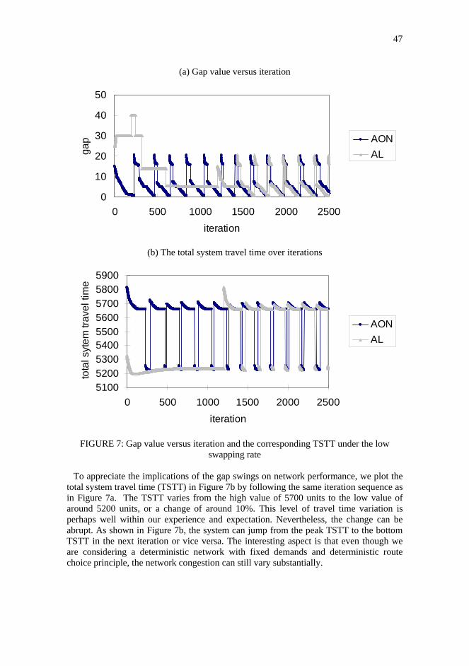
Figure 7a shows the gap value over time (or from iteration to iteration) under the low

swapping rate. In general, the gap value does not monotonically decrease with time. Instead, after a certain period, the gap increases and decreases periodically with a nearly constant cycle. Examining the detailed traffic results, the large increase in the gap value can be attributed to the effect of junction blockage. The phenomenon of blockage, which is depicted by physical-queue traffic models and happens in reality, can lead to substantial changes in the route travel times even with a small change in the flow pattern (proposition 1 in section 2). This implies that the current shortest route can become an unacceptable route in the next iteration, leading to a large gap. Based on this limited experiment, it is not clear whether this periodic behaviour shall always occur in the absence of a tolerance-based DUO solution. We leave the more exact and detailed treatment of this phenomenon to a future study.

Figure 7a also illustrates that the choice of the initial solutions (AON or AL) affects the gap values of the early iterations. As the algorithm proceeds to a substantial number of iterations (1500 iterations for the small swapping rate and 5 iterations (not shown here due to the space limitation) for the high swapping rate), essentially the gap values produced by the different initial solutions show no appreciable differences. Both cases follow a similar periodic pattern of gap oscillation. Based on this limited experiment, it appears that the choice of the initial solutions does not have a substantial impact on the final evolving traffic pattern. On the other hand, the length of the periodicity is related to the swapping rate. For a low swapping rate, as seen from Figure 7a, it takes around 200+ iterations to complete a cycle; whereas for the case of a high swapping rate (not shown here), it just takes around 10 iterations. If we interpret the iterations as a day-to-day route adjustment process, more aggressive swapping behaviors lead to more frequent oscillations in network performance.

47

(a) Gap value versus iteration

0

10

20

30

40

50

0 500 1000 1500 2000 2500iteration

gap AON

AL

(b) The total system travel time over iterations

510052005300540055005600570058005900

0 500 1000 1500 2000 2500iteration

tota

l syt

em tr

avel

tim

e

AONAL

FIGURE 7: Gap value versus iteration and the corresponding TSTT under the low

swapping rate To appreciate the implications of the gap swings on network performance, we plot the

total system travel time (TSTT) in Figure 7b by following the same iteration sequence as in Figure 7a. The TSTT varies from the high value of 5700 units to the low value of around 5200 units, or a change of around 10%. This level of travel time variation is perhaps well within our experience and expectation. Nevertheless, the change can be abrupt. As shown in Figure 7b, the system can jump from the peak TSTT to the bottom TSTT in the next iteration or vice versa. The interesting aspect is that even though we are considering a deterministic network with fixed demands and deterministic route choice principle, the network congestion can still vary substantially.

48

7. SUMMARY AND FUTURE RESEARCH DIRECTIONS 7.1 Summary

Other than the important findings on DTA properties and their implications, the major contributions of the thesis by Szeto (2003) is to provide some initial thinking on developing a framework to accommodate the possible non-existence of perfect DUO equilibrium solutions to the DTA problem under the physical queue paradigm. The proposed extension or relaxation is actually more reflective of our actual experience, as perfect DUO is an idealization anyway. Specifically, the thesis develops a route choice principle based on the notion of bounded rationality, namely tolerance-based DUO, and a modified route-swapping heuristic for solutions. The existence of a stable solution depends on the network topology and demand pattern, and also travellers’ behaviour on travel time tolerance. The thesis demonstrates that for a small tolerance, the system can keep on evolving without converging to a stable equilibrium, meaning that equilibrium traffic assignment is not an intrinsic property to every network. Therefore, the generalized notion of “non-equilibrium dynamic traffic assignment” is necessary to describe certain networks when traffic is represented with the more realistic physical queue paradigm. 7.2 Future research directions

Many research directions are possible. Some are identified as below:

7.2.1 Travel choice principle As seen in the numerical study, in the absence of equilibrium, the traffic pattern may

keep on evolving. Of particular interest are the stability and periodicity of the changing traffic pattern. The numerical study showed that the change in overall network travel time can be rather abrupt, with its magnitude of change lying within a limit of around 10%, which is perhaps consistent with our experience and expectation. Yet theoretical explorations of the network behaviour under non-equilibrium, bounds of the changes in the total system travel time, periodicity of the changes, and their relations to the travellers’ aggressiveness in route swapping, etc. are interesting and important questions to be answered in future research. The thesis only provides an initial step toward this direction. Alternatively, one may develop other travel choice principles that are behaviourally sound and consistent with actual travel behaviour.

7.2.2 Traffic flow modelling

Lo and Szeto (2002a) modelled the traffic-flow component as a unique mapping

yielding route travel times given route flows, which allows the encapsulation of a range of dynamic traffic flow models in DTA. One can employ car-following simulation traffic flow models, continuum traffic flow models, and others in this mapping as long as they can produce a unique mapping between the route travel times and route flows through their route travel time extraction procedure. One can develop advanced traffic flow models based on these existing traffic flow models to capture realistic traffic behaviours such as shockwaves, queue formulation and dissipation, and queue spillback, lane

49

changing behaviour, hysteresis phenomenon, etc., and use the unique mapping to encapsulate the advanced traffic flow models in a DTA framework. 7.2.3 Link travel time functions

Encapsulating an entire traffic flow model using the unique mapping can greatly

improve the solution quality, but at the same time increases the computation effort, as repeated traffic simulations are required to update the route travel times from iteration to iteration. Therefore, the question is how to speed up the solution process. Can we adopt travel time functions to approximate the unique mapping at some stages inside the computations to speed up the solution processes? Can this guarantee convergence? Alternatively, will there be sufficiently refined (even though not perfectly correct) travel time functions to replace the approach of encapsulating an entire traffic flow model? This approach will have tremendous saving in computational time. 7.2.4 Parallel computing

As mentioned before, with the encapsulating of the effects of physical queues in DTA,

one can only rely on less restrictive algorithms such as genetic algorithms to solve the physical-queue DTA models. However, genetic algorithms have to evaluate the objective values of each trial solution, which is a time-consuming process. This is especially true if the objective function is complicated; say the objective function includes the whole traffic simulation model. To increase the computation efficiency, a possible approach is implementing parallelized genetic algorithm (e.g., Wong et al., 2001) for solving these models. This approach makes good use of the inherent nature of genetic algorithms that the evaluation of each trial solution can be done independently, and hence the performance of genetic algorithms can be greatly improved by means of parallel computing. 7.2.5 Time-dependent path set generation

A large network involves many paths, although most would not be used. A large path

set makes path enumeration impossible. However, to deal with queue spillback properly, we must use path-based DTA models and hence path-based algorithms. One possible approach to deal with the large path set is to generate a small path set in the path-based solution algorithm. Compared with the path-based solution algorithms for static models, an additional effort on the path set generation for DTA models is required because we need to consider time-dependent paths. In particular, the effect of junction blockages can cause the network configuration temporally change, which must be duly handled. This raises questions: Can the path set generation rules used in the static traffic assignment be modified and extended to the dynamic case? Are there any other methods to efficiently deal with the temporally changing network configuration under the effects of physical queues? How does the choice of path set generation rules affect the solution speed and convergence of the algorithm? These questions require further study. 7.2.6 Framework for online applications

One of the applications of DTA models is to predict the real time traffic flow and

update the time-dependent OD matrix for online application purposes. Existing literature

50

focuses on using simulation DTA models or analytical point queue DTA models for this purpose. Simulation models cannot guarantee the solution optimality; Point queue models cannot capture the effect of physical queues. Developing a framework using physical-queue DTA models for this purpose is definitely another research direction. For this issue, one can improve the framework for non-congested networks proposed by Ran et al. (2002a) to congested networks wherein junction blockage is common. 7.2.7 Solution approaches

There are a number of solution approaches, including swapping algorithms (e.g., Smith

and Wisten, 1995; Huang and Lam, 2002), projection methods (e.g., Lo and Szeto, 2002a, 2004, 2005; Szeto and Lo, 2004), genetic algorithms (e.g., Lo and Szeto, 2002b), diagonalization algorithm (Ran et al., 2002b), and method of successive averages (e.g., Tong and Wong, 2000). Which approach is more efficient for solving physical-queue DTA models? Which approach can guarantee convergence under the physical-queue consideration? How do the parameters in the algorithms affect the efficiency and convergence? These questions are worthwhile future research topics. 7.2.8 Model calibration and validation

The evaluation and prediction from DTA models rely heavily on how well they

represent the actual traffic. Therefore DTA models must be calibrated and validated, both for the traffic-flow component and the travel choice principle. However, traffic data are full of noise. Gathering wrong data definitely affects the prediction and evaluation results. How should we employ the traffic data with noise to calibrate traffic flow models or the link performance functions? What is the methodology to validate the proposed travel choice principle? These questions must be duly considered before applying the models for evaluation, planning, and operations.

All the above research directions are equally important from the practical and

theoretical point of views. The authors are currently tackling some of the above.

ACKNOWLEDGEMENT We are grateful to the members of the thesis committee, including Prof. William Hing

Keung Lam, Prof. Hai Yang, Dr. Sze Chun Wong, and Dr. Jiyin Liu for reviewing the thesis and providing their valuable comments and suggestions for improving its quality. We also thanks for the referees for constructive comments. This research is sponsored by the Competitive Earmarked Research Grant HKUST6283/04E from the Hong Kong Research Grant Council.

REFERENCES

Adamo, V., Astarita, V., Florian, M., Mahut, M. and Wu, J.H. (1999) Modeling the

spillback of congestion in link based dynamic network loading models: A simulation model with application. In A. Ceder (Ed.), Transportation and Traffic Theory, Pergamon-Elsevier, New York, pp. 555-573.

51

Astarita, V. (1996) A continuous time link model for dynamic network loading models based on travel time function. In J.B. Lesort (ed.), Transportation and Traffic Theory, Pergamon-Elsevier, New York, pp. 79-102.

Carey, M. (1992) Nonconvexity of the dynamic traffic assignment problem. Transportation Research Part B, 26, 127-133.

Carey, M., Ge, Y.E. and McCartney, M. (2003) A whole-link travel time model with desirable properties. Transportation Science, 37, 83-96.

Daganzo, C.F. (1994) The cell transmission model: A simple dynamic representation of highway traffic. Transportation Research Part B, 28, 269-287.

Daganzo, C.F. (1995) The cell transmission model, Part II: Network traffic. Transportation Research Part B, 29, 79-93.

Friesz, T.L., Bernstein, D.H., Smith, T.E., Tobin, R.L. and Wie, B.W. (1993) A variational inequality formulation of the dynamic network user equilibrium problem. Operations Research, 41, 179-191.

Friesz, T.L., Cho, H.J., Mehta, N.J., Tobin, R.L. and Anandalingam, G. (1992) A simulated annealing approach to the network design problem with variational inequality constraints. Transportation Science, 26, 18-26.

Heydecker, B.G. and Addison, J.D. (1998) Traffic models for dynamic traffic assignment. In M.G.H. Bell (ed.) Transport Networks: Recent Methodological Advances, Pergamon-Elsevier, Oxford, pp. 35-49.

Hu, T. and Mahmassani, H.S. (1997) Day-to-day evolution of network flows under real-time information and reactive signal control. Transportation Research Part C, 5, 51-69.

Huang, H.J. and Lam, W.H.K. (2002) Modeling and solving dynamic user equilibrium route and departure time choice problem in network with queues. Transportation Research Part B, 36, 253-273.

Jayakrishnan, R., Mahmassani, H.S. and Hu, T.Y. (1994) An evaluation tool for advanced traffic information and management systems in urban networks. Transportation Research Part C, 2, 129-147.

Jayakrishnan, R., Tsai, W.K. and Chen, A. (1995) A dynamic traffic assignment model with traffic flow relationship. Transportation Research Part C, 3, 51-82.

Kuwahara, M. and Akamatsu, T. (2001) Dynamic user optimal assignment with physical queues for a many-to-many OD pattern. Transportation Research Part B, 35, 461-479.

Lo, H.K. (1999) A dynamic traffic assignment formulation that encapsulates the cell transmission model. In A. Ceder (ed.) Transportation and Traffic Theory, Pergamon, Oxford, pp. 327-350.

Lo, H.K. and Szeto, W.Y. (2002a) A cell-based variational inequality formulation of the dynamic user optimal assignment problem. Transportation Research Part B, 36, 421-443.

Lo, H.K. and Szeto, W.Y. (2002b) A cell-based dynamic traffic assignment model: formulation and properties. Mathematical and Computer Modeling, 35, 849-865.

Lo, H.K. and Szeto, W.Y. (2004) Modeling advanced traveler information services: Static versus dynamic paradigms. Transportation Research Part B, 38, 495-515.

Lo, H.K. and Szeto, W.Y. (2005) Road pricing modeling for hyper-congestion. Transportation Research Part A, in press.

Mahmassani, H.S. and Chang, G.L. (1987) On boundedly rational user equilibrium in transportation systems. Transportation Science, 21, 89-99.

Mahmassani, H.S. and Liu, Y.H. (1999) Dynamics of commuting decision behaviour under advanced traveler information systems. Transportation Research Part C, 7, 91-107.

52

Nagurney, A. (1993) Network Economics: A Variational Inequality Approach. Kluwer Academic Publishers, Norwell, Massachusetts, USA.

Ran, B. and Boyce, D. (1996) Modeling Dynamic Transportation Networks. An Intelligent Transportation System Oriented Approach. Second Revised Edition. Springer-Verlag, Heidelberg.

Ran, B., Lee, D.H. and Shin, M.S.I. (2002a) Dynamic traffic assignment with rolling horizon implementation. Journal of Transportation Engineering, ASCE, 128, 314-322.

Ran, B., Lee, D.H. and Shin, M.S.I. (2002b) New algorithm for a multiclass dynamic traffic assignment model. Journal of Transportation Engineering, ASCE, 128, 323-335.

Rubio-Ardanaz, J.M., Wu, J.H. and Florian, M. (2001) A numerical analytical model for the continuous dynamic network equilibrium problem with limited capacity and spill back. 2001 IEEE Intelligent Transportation Systems Conference Proceedings, pp. 263-267.

Simon, H. (1955) A behavioural model of rational choice. The Quarterly Journal of Economics, 69, 99-118.

Smith, M.J. (1993) A new dynamic traffic model and the existence and calculation of dynamic user equilibria on congested capacity-constrained road networks. Transportation Research Part B, 27, 49-63.

Smith, M.J. and Wisten, M.B. (1995) A continuous day-to-day traffic assignment model and the existence of a continuous dynamic user equilibrium. Annals of Operations Research, 60, 59-79.

Szeto, W.Y. (2003) Dynamic Traffic Assignment: Formulations, Properties, and Extensions. PhD Thesis, The Hong Kong University of Science and Technology, H.K.

Szeto, W.Y. and Lo, H.K. (2004) A cell-based simultaneous route and departure time choice model with elastic demand. Transportation Research Part B, 38, 593-612.

Tong, C.O. and Wong, S.C. (2000) A predictive dynamic traffic assignment model in congested capacity-constrained road networks. Transportation Research Part B, 34, 625-644.

Wardrop, J. (1952) Some theoretical aspects of road traffic research. Proceedings of the Institute of Civil Engineers, Part II, 325-378.

Yang, H. and Meng, Q. (1998) Departure time, route choice and congestion toll in a queuing network with elastic demand. Transportation Research Part B, 32, 247-260.

Wong, S.C., Wong, C.K. and Tong, C.O. (2001) A parallelized genetic algorithm for calibration of Lowry model. Parallel Computing, 27, 1523-1536.

Ziliaskopoulos, A.K., Waller, S.T., Li, Y. and Byram, M. (2004) Large-scale dynamic traffic assignment: implementation issues and computational analysis. Journal of Transportation Engineering, ASCE, 130, 585-593.