Short-term traffic predictions on large urban traffic networks: applications of network-based machine learning models and dynamic traffic assignment models

2015 Models and Technologies for Intelligent Transportation Systems (MT-ITS) 3-5. June 2015. Budapest, Hungary

978-963-313-142-8 @ 2015 BME

Short-term traffic predictions on large urban traffic networks: applications of network-based machine learning models and dynamic traffic assignment

models Gaetano Fusco, Chiara Colombaroni, Luciano Comelli, Natalia Isaenko

Department of Civil, Constructional and Environmental Engineering Sapienza University of Rome

Rome, Italy [email protected], [email protected], [email protected], [email protected]

Abstract—The paper discusses the issues to face in applications of short-term traffic predictions on urban road networks and the opportunities provided by explicit and implicit models. Different specifications of Bayesian Networks and Artificial Neural Networks are applied for prediction of road link speed and are tested on a large floating car data set. Moreover, two traffic assignment models of different complexity are applied on a sub-area of the road network of Rome and validated on the same floating car data set.

Keywords—Short-term traffic predictions, Floating Car Data, Bayesian Networks, Neural Networks, Dynamic Traffic Assignment

I. INTRODUCTION

Predicting future traffic conditions in real-time is a crucial issue for applications of Intelligent Transportation Systems (ITS) devoted to traffic management and traveler information. Traditional traffic monitoring systems are based on fixed measure stations where flows, occupancy and possibly speed are detected. Collected data are then transmitted to the traffic control center, where they are processed to derive short-term predictions. These can be performed by applying either implicit models, which derive future values on the basis on the observed trend of the variables (so-called ‘data-driven’ models), or explicit models, which predict future traffic values by simulating the traffic network along a rolling horizon time window. The high cost of fixed monitoring system was one of the most relevant limiting factors for a full ITS deployment although efficient algorithms for optimizing sensor locations were developed [1]. The wide diffusion of Floating Car Data collected by probe vehicles open new perspectives to develop novel predicting models. In fact, they provide a pervasive tool to explore the network and get information related to theoretically any point of the network [2] and, in a near future, perform self-organizing monitoring techniques ([3]-[4]). The drawback is that the information comes from only a sample of vehicles that send their current position and speed. Thus, they provide ubiquitous but partial information. This fact implies a supplementary effort to interpret these data and combine the information collected in different points and different instants.

Implicit data-driven models derive predictions on future traffic states from past observed trends. Space relations are often neglected, although network-based machine learning models like Artificial Neural Networks and Bayesian Networks can be formulated to reflect the topology of the network and then to exploit larger correlations between measures collected on close links [5]. However, these models do not reproduce the physical nature of traffic and cannot capture, for example, the diffusion of queues to an upstream link that affects the performances of that link abruptly. The question is to investigate the capabilities of the network-based machine learning models to reflect the nature of the spatio-temporal relationships that characterize traffic on the urban road networks and provide reliable traffic prediction.

Explicit models have been object of a great research effort by the academic community, which developed in the last three decades more and more complex dynamic traffic assignment models that simulate the road network behavior with great detail and level of realism. However, explicit modeling requires a huge effort to collect all data needed as inputs and then to calibrate the model. Specifically, deriving reliable time-dependent origin-destination demand in real-time is a very challenging task, which requires detailed and frequently updated traffic data. On the other hand, while implicit models are usually applied on a very limited set of links, explicit models provide results on all links of the network simultaneously. Also, dynamic traffic assignment models have the great advantage that they can simulate the effects of information strategies and can predict network performances in non-standard conditions. However, they are not scalable and they are not generalizable from one application to another. Finally, a convenient approach to traffic prediction could consist in exploiting the complementary features of the two kinds of models and combine them in an integrated framework.

In this paper, we analyze and compare implicit and explicit approaches for travel time prediction on a large road network. The experimental tests of different models are addressed to assess the following issues: accuracy of predictions; calibration

2015 Models and Technologies for Intelligent Transportation Systems (MT-ITS) 3-5. June 2015. Budapest, Hungary

978-963-313-142-8 @ 2015 BME

efforts; reliability of measures. This paper is organized as follows. Section 2 provides a brief review of related work on short-term forecasting methods. The proposed prediction methods based on two different implicit models are described in Section 3. The objectives and main results of the application of both implicit and explicit models in a real test case are presented in Section 4. Conclusions follow.

II. RELATED WORK

A huge literature exists on short-term traffic forecasting. A complete review of the state-of-the art is out of the scope of this work and can be found in two very recent papers, presented by Vlahogianni et al. [6] and Ho et al. [7]. Taxonomy of different approaches reported in literature is provided by Van Hinsbergen et al. as a practical reference for ITS professionals and researchers [8]. In this paper we are interested in investigating the potentials of implementation of Bayesian Networks to short-term traffic forecasting in comparison with other state-of-art implicit and explicit models. Thus, we focus our review on this more specific issue.

Bayesian Networks (BN) were applied for traffic flow forecasting firstly by Sun et al. [9], who proposed a graphical model containing information from neighbor links and an expanded model containing information from further links to deal with missing data. The results showed that BN model outperforms other consolidated methods such as Random Walk (information concerning only current traffic flow condition), AR model and a fuzzy-neural model. In case of partial evidence (i.e. when some link flows are known) the variance of other parameters reduces, leading to better model performances. The Bayesian Network method enhances the link flows relations by conditional distributions providing thus more information respect to classical matrix estimation methods. Hofleitner et al. developed a graphical model connecting travel times with congestion state of each road link and a traffic theoretical model that reproduces the distribution of delay within a road segment [10]. The two models were combined into a Dynamic Bayesian Network, which demonstrated to highly exceed performances provided by a time-series model for travel time estimation. Combinations of various techniques and use of multiple predictors have recently become a point of interest. Hybrid structures usually involve Neural Networks and other predictors; the credits associated to predictors depend on the performances of the predictors in the preceding time intervals. The results show better accuracy and stability of integrated methods respect to single predictors (see, among others, [11], [12], [13]). The nature of traffic congestion implicates that the computational methodologies of artificial intelligence must be transportation-inspired.

In this paper we move on this direction and we integrate a consolidated Seasonal ARIMA model into a Bayesian Network as an a priori estimator. The specification of model variables tries to exploit all the available information about a traffic state; thus, variances between individual velocities as well as flow estimations are taken into account. The underline assumption is that a high mean speed with a high variance may indicate that the traffic conditions moved to unstable state. On

the other hand, a low number of FCD counts could compromise measurement reliability and should be taken into account. Time-space evolution of a traffic flow state is extremely important in traffic engineering since it enables better understanding of traffic dynamics. The propagation of a traffic state is taken into account by considering neighbor links.

III. PREDICTION METHODS BASED ON IMPLICIT MODELS

A. Time series analysis (ARIMA)Autoregressive Integrated Moving Average (ARIMA) is

one of the most consolidated methods for time-series forecasting, used in various fields and introduced in traffic forecast on freeways since late ‘70s [14]. The forecast provided by the model is a linear combination of past observations multiplied by coefficients reflecting autoregressive (AR) and moving average (MA) nature of the process. In case the time series displays a trend the data must be differenced thus the integration term (I) is usually introduced for making the time series stationary. Whether the time series presents seasonality additional SAR, SMA terms are introduced. Various seasonal ARIMA models were applied in traffic engineering for traffic state prediction ([15], [16]). In this study, we applied seasonal ARIMA (SARIMA in the following) to catch time periodicity of speed data detected on road network links.

B. Artificial Neural NetworksAmong the numerous previous examples already in

literature, two architectures of artificial Neural Networks are considered in this study: Feed-Forward (FF) and Non-linear Auto-Regressive model with exogenous inputs (NARX). The former is a static nonlinear vector multivariate function that relates future values of speed v(t+1) on an output link to the observed values of traffic variables u(t, t–1,…, t–k)={u1(t, t–1,…, t–k),…um(t, t–1, …, t–k)} detected in k previous time intervals on links 1, 2,…m, including the output one.

where t is the current time interval, k is the number of previous time intervals taken into consideration, u is the input vector, z is a vector representing the output of the hidden layer, fc is a nonlinear activation function, B and C are coefficient matrices, ϑC and ϑD are threshold values associated to the output and hidden layers, respectively. A graphical representation of the architecture of the FF Neural Network is depicted in Fig.1.

Fig. 1. Architectural graph of the Feed-Forward Neural Network

v t +1( ) = fc Cz +ϑC( )z = fc Bu t1, t −1, t − k( ) +ϑD( )

x1 (t) x2 (t) ….. x5 (t) y (t)

y (t+1)

2015 Models and Technologies for Intelligent3-5. June 2015. Budapest, Hungary

978-963-313-142-8 @ 2015 BME

NARX is a recurrent Neural Network that rvalues of speed on the output link v(t+1) to prtraffic variables on other links {v2(t, t–1,…, …, t–k)} and on the same link v(t, t–1,…, t–k)delay line connections that provide delayed vbe used in short-term predictions (Cfr. Fig.2):

with the same meaning of the symbols antransfer function. Fig.2 provides the rerepresentation.

Fig. 2. Architectural graph of the Non-linear Auto-Regexogenous inputs Neural Networ

C. Bayesian NetworksBayesian Networks (BN) are probab

models. This definition outlines the two compbe specified in a BN: a graphical component, directed acyclic graph, and a probabiliexpressed by probability distributions. In partof the graph represents a random variable, whconnect the nodes represent probabilistibetween the corresponding random variables. relations used in BNs can be represented byneighbor links in case of traffic dynamics.

Fig.3 illustrates the BN used here for forecasting. The speed at time t+τ is the eswhile other nodes represent the conditioninassume that traffic state at time t+τ depends utraffic state on the estimated link and upon thstates on the conditioning links. The conditrepresented by the backward star (which shostable traffic conditions) and the forward star (active in spill-back congestion propagation) link. Traffic variables u on conditioning linksand other available measures of variables thattraffic pattern, such as FCD observations nustandard deviation of individual speed σ. A SAintegrated into the BN as an a priori estimator.

v t +1( ) = f v t( ), v t −1( ), , v t − k( ), u t( ), u t −((

x (t) x (t-1) x (t-2) ….. x (t-4)

y (t) y (t-1) y (t-2) ….. y (t-4)

t Transportation Systems (MT-ITS)

relates the future revious values of t–k),…vm(t, t–1,

), through tapped values of speed to

nd f a nonlinear elated graphical

gressive model with rk

bilistic graphical ponents that must

represented by a stic component,

ticular, each node hile the links that ic dependencies The cause-effect

y considering the

short-term speed timated variable,

ng variables. We upon the previous e previous traffic tioning links are ould be active in (which should be of the estimated

s include speed v t characterize the

umber n, and the ARIMA model is .

Fig. 3. Bayesian Network structure wit

The expected advantage of prenetwork architecture, such as NeurNetwork, is that their graph stcapability to catch the time-depentraffic states on the road netwspecifications were preliminary studthe time-space correlation among dnetwork. Both upstream and dprediction link were included to takeflow progression that occurs in lprogression that arises in congestedinvolved different numbers of upstrThe best trade-off between complexaccuracy of predictions was provicomposed by the link itself, the bacstar. This structure has also two greamodular and can be easily implemthrough simple automatic routines tand select the forward star of end nof initial node for each prediction lin

IV. APPLICATION TO

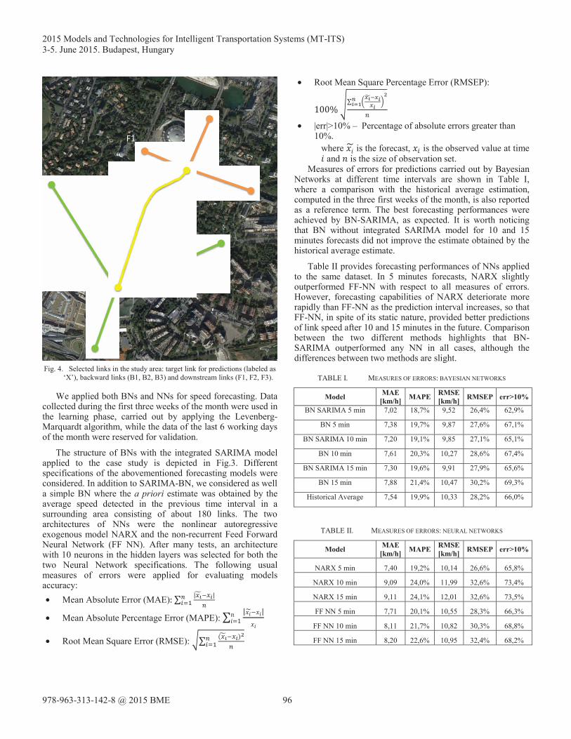
A. Sparse FCD data (5-minute aggThe study area is a road netwo

area of Rome, where a large databacollecting system was available. Evand speed of an individual vehicle, da single FCD point. We aggregated intervals aggregation and averagemean speed estimation. Input variaconsist of: average speed, numbestandard deviation of speeds of indfor every 5-minute time interval. selected a small set of links, aspredictions of speed on a link x forare obtained by taking detected speand 3 downstream links as input. Ovvalues on the subset of links and 5prediction link collected during May

−1), u t − k( ))

y (t+1) th a priori SARIMA estimator

ediction methods based on ral Networks and Bayesian tructure should have the ndent spatial correlation of ork. Several architectural died and tested to represent different links on the road

downstream links of the e into account both forward light traffic and spillback

d conditions. Different tests eam and downstream links. xity of the architecture and ided by a simple structure ckward star and the forward at practical advantages: it is mented on large networks that explore the road graph node and the backward star nk.

O A CASE STUDY

gregation) rk situated in the Southern

ase of FCD based on a GPS very observation of position detected every 2 minutes, is the data into 5-minute time

ed single observations for ables for predicting models r of observations and the

dividual vehicles, computed For test applications we

s shown in Fig.4, where r next 5, 10 and 15 minutes eeds from 3 upstream links ver 370,000 observed speed 54,000 observations on the y of 2010 were available.

2015 Models and Technologies for Intelligent Transportation Systems (MT-ITS) 3-5. June 2015. Budapest, Hungary

978-963-313-142-8 @ 2015 BME

Fig. 4. Selected links in the study area: target link for predictions (labeled as ‘X’), backward links (B1, B2, B3) and downstream links (F1, F2, F3).

We applied both BNs and NNs for speed forecasting. Data collected during the first three weeks of the month were used in the learning phase, carried out by applying the Levenberg-Marquardt algorithm, while the data of the last 6 working days of the month were reserved for validation.

The structure of BNs with the integrated SARIMA model applied to the case study is depicted in Fig.3. Different specifications of the abovementioned forecasting models were considered. In addition to SARIMA-BN, we considered as well a simple BN where the a priori estimate was obtained by the average speed detected in the previous time interval in a surrounding area consisting of about 180 links. The two architectures of NNs were the nonlinear autoregressive exogenous model NARX and the non-recurrent Feed Forward Neural Network (FF NN). After many tests, an architecture with 10 neurons in the hidden layers was selected for both the two Neural Network specifications. The following usual measures of errors were applied for evaluating models accuracy: • Mean Absolute Error (MAE)

• Mean Absolute Percentage Error (MAPE):

• Root Mean Square Error (RMSE):

• Root Mean Square Percentage Error (RMSEP):

• |err|>10% – Percentage of absolute errors greater than 10%.

where is the forecast, is the observed value at time and is the size of observation set.

Measures of errors for predictions carried out by Bayesian Networks at different time intervals are shown in Table I, where a comparison with the historical average estimation, computed in the three first weeks of the month, is also reported as a reference term. The best forecasting performances were achieved by BN-SARIMA, as expected. It is worth noticing that BN without integrated SARIMA model for 10 and 15 minutes forecasts did not improve the estimate obtained by the historical average estimate.

Table II provides forecasting performances of NNs applied to the same dataset. In 5 minutes forecasts, NARX slightly outperformed FF-NN with respect to all measures of errors. However, forecasting capabilities of NARX deteriorate more rapidly than FF-NN as the prediction interval increases, so that FF-NN, in spite of its static nature, provided better predictions of link speed after 10 and 15 minutes in the future. Comparison between the two different methods highlights that BN-SARIMA outperformed any NN in all cases, although the differences between two methods are slight.

TABLE I. MEASURES OF ERRORS: BAYESIAN NETWORKS

Model MAE [km/h] MAPE RMSE

[km/h] RMSEP err>10%

BN SARIMA 5 min 7,02 18,7% 9,52 26,4% 62,9%

BN 5 min 7,38 19,7% 9,87 27,6% 67,1%

BN SARIMA 10 min 7,20 19,1% 9,85 27,1% 65,1%

BN 10 min 7,61 20,3% 10,27 28,6% 67,4%

BN SARIMA 15 min 7,30 19,6% 9,91 27,9% 65,6%

BN 15 min 7,88 21,4% 10,47 30,2% 69,3%

Historical Average 7,54 19,9% 10,33 28,2% 66,0%

TABLE II. MEASURES OF ERRORS: NEURAL NETWORKS

Model MAE [km/h] MAPE RMSE

[km/h] RMSEP err>10%

NARX 5 min 7,40 19,2% 10,14 26,6% 65,8%

NARX 10 min 9,09 24,0% 11,99 32,6% 73,4%

NARX 15 min 9,11 24,1% 12,01 32,6% 73,5%

FF NN 5 min 7,71 20,1% 10,55 28,3% 66,3%

FF NN 10 min 8,11 21,7% 10,82 30,3% 68,8%

FF NN 15 min 8,20 22,6% 10,95 32,4% 68,2%

X

B3

B2

B1

F1 F2

F3

2015 Models and Technologies for Intelligent3-5. June 2015. Budapest, Hungary

978-963-313-142-8 @ 2015 BME

The results of the validation phase are depiform in Fig.5, where observed data for the lasof the month are reported together with 5 mifrom BN-SARIMA and FF NN. In the picnoticing the big noise of measures and goodness-of-fit of both forecasting models.

A detail of the results obtained in a singMay) is exemplified for BN-SARIMA, FF-NFig.6, where the observed speeds and the interval of the estimated average value arAlthough the number of observations on the pone day was in the order of several hundreds, time intervals where very few data were avaiconfidence interval is irregular and often veorder of ten of km/h). It is obvious that measlarge confidence intervals are not statisticallycannot taken as reference for validation ofmodels. Thus, the validation of the results shoumeasure that matches the forecasted values wiinterval other than computing their square difaverage value. In the whole validation set, pminute intervals provided by NARX and SAwithin the 90% confidence interval in about 78% of the observations, respectively.

Fig. 5. Observed values of speed and corresponding 5 from BN-SARIMA and FF-NN (6 days used

Variance of measured speed and number ofor every time interval should be included intoerrors to evaluate the forecasting capability orespect to the reliability of measures and withintrinsic variance of the phenomenon measurements are collected or their varianestimated mean value is affected by high unwe introduced a new measure of errors thconfidence level (1–α) of the average observedconfidence interval (±5%xi), where xi is thespeed obtained from l FCD observations in eaThe value of the corresponding level of cdepends upon sample size l and sample standMultiplying the absolute error by the confide

t Transportation Systems (MT-ITS)

icted in graphical st 6 working days nutes predictions cture it is worth the overall fair

gle day (28th of NN and NARX in

90% confidence re also reported. prediction link in there were single ilable, so that the ery large (in the sures having very y significant and f the forecasting uld include also a th the confidence fference with the

predictions for 5-ARIMA BN fell the 79% and the

minute predictions for validation).

of FCD collected o the measures ofof the model with h reference to the

(i.e., if few nce is high, the ncertainty). Thus, hat considers the d speed. We set a e observed mean ach time interval. confidence (1–α) dard deviation σ. ence level of the

measured speed we obtain a weighencompasses estimation reliability onew index Reliability-Weighted (RMAE):

In order to focus on large predithe corresponding reliability of thethe indicator ACL(err>10%) that cwith magnitude greater than 10% confidence level of the correspondingiven confidence interval (±5%xi).

Fig. 6. Predictions from SARIMA-BN anintervals and observed values of spe

interval with 90%

Table III and Table IV show thefor different time interval pspecifications of Bayesian Networrespectively. Results of Table III hiamong different specifications werspecifications outperformed the simshown in Table IV, NARX provpredictions as those achieved byobtained by Neural Networks hacompare the results of Table III witnotice that 15–minute predictions (BN 15) had a higher percentage othose that would had been obtainehistorical average of speed observedHowever, the large errors made by were less reliable (ACL=15.8%) thhistorical average (ACL=16.2).

hted measure of errors that of observations. We call this

Mean Absolute Error

ction errors with respect to e measures, we introduced ounts all predictions errors and computes the average ng measures of speed, for a

nd FF-NN models for 5 minute eed with the related confidence

% probability.

e values of these indicators redictions and different rks and Neural Networks, ighlight that the differences re very slight and all BN

mple statistical estimate. As vided as reliable 5–minute y BN, while other results d lower reliability. If we th those of Table I, we can of the Bayesian Network

f large errors (69.3%) than ed by simply applying the d on that road link (66.0%). BN 15 occurred when data an those made by applying

2015 Models and Technologies for Intelligent Transportation Systems (MT-ITS) 3-5. June 2015. Budapest, Hungary

978-963-313-142-8 @ 2015 BME

TABLE III. RELIABILITY-WEIGHTED MEASURES OF ERRORS: BAYESIAN NETWORKS

Model RMAE [km/h] ACL(err>10%)BN SARIMA 5 min 1,13 15,8%

BN 5 min 1,08 15,8%

BN SARIMA 10 min 1,08 15,8%

BN 10 min 1,14 15,7%

BN SARIMA 15 min 1,09 15,6%

BN 15 min 1,19 15,8%

Historical Average 1,21 16,2%

TABLE IV. RELIABILITY-WEIGHTED MEASURES OF ERRORS: NEURAL NETWORKS

Model RMAE [km/h] ACL(err>10%)

NARX 5 min 1,12 15,8%

NARX 10 min 1,39 16,4%

NARX 15 min 1,39 16,4%

FF NN 5 min 1,19 15,9%

FF NN 10 min 1,22 15,7%

FF NN 15 min 1,23 15,8%

B. Sparse FCD data (15-minute aggregation)Validation of prediction results is strongly affected by the

aggregation over time of the data; that is, by the desired precision of the estimate. It is interesting to compare the accuracy of speed predictions obtained at the generic time interval t for the 5–minute interval from 10 to 15 minutes after t with the predictions for the next 15–minute interval obtained from data aggregated with the same 15–minute granularity. Thus, we applied the two least performing specifications of the two methods, that is the standard BN without SARIMA a priori estimate and a NARX model, to the same FCD data with 15–minute data aggregation. As expected, reducing precision of the estimates increases their accuracy. Results shown in Table V exhibit significantly lower values for all measures of errors (RMSE around 8.3km/h; RMSEP around 22%) with respect to the corresponding values obtained for 5–minute aggregation (RMSE around 10.5km/h; RMSEP around 30.2% in the best case, that is the Bayesian Network).

TABLE V. MEASURES OF ERRORS: NNS AND BNS (15-MINUTES DATA)

Model MAE

[km/h] MAPE RMSE [km/h] RMSEP

BN 5,95 15,4% 8,25 21,9%

NARX 6,10 15,1% 8,36 21,6%

C. Aggregated TomTom databaseThe same analysis was conducted on a different database,

consisting on speed estimation measures supplied by TomTom, which were made available for the research project. From a large database of link speed covering the whole town of Rome for about 7 months, several sub-areas were chosen and both BN and NN prediction methods were applied on some selected links. Results obtained were almost stable for different areas, although they were taken in different central or peripheral areas of the town. To allow a comparison with tests shown in Sections A and B, results obtained on the same links are shown in the following. A more detailed analysis of tests carried out to define the best architecture of the models and an extensive description of the results experienced in the applications is reported in a contemporary paper of the same authors [20].

Unlike the set of FCD discussed in the previous section, TomTom data contained only aggregate estimates of speed on links and did not indicate the number of counts. Anyway, they contained a confidence factor that expresses an informal degree of belief in the reliability of the estimated values of the average link speed, aggregated with 5–minute time intervals. A BN without an a priori estimation and two NNs were applied to aggregated data. Training phase was carried out on the 70% of the sample. The remaining 30% was used for the validation. In a first test, result validation was limited to the subset of data that had the highest score of degree of belief, while the training was performed on all available data of the training set. In a second test the whole dataset was used for both training and validation, without any selection of the most reliable data.

Table VI refers to validation performed on the most reliable subset of data. Results show that the RMSE ranged from about 5.6km/h to about 7.1km/h, which are significantly lower values than those obtained in the experiment conducted on the database of individual speed described in Section A (ranging approximately from 9.5km/h to 12.0 km/h). However, the RMSEP values (from 23.8% to 34.2%) encompass the range experienced by the former experiment (26.4% to 32.6%), because the estimation of the average speed provided by TomTom was on average lower than that estimated from the former database of individual speed.

TABLE VI. MEASURES OF ERRORS: BNS AND NNS (TOMTOM DATA)

Model MAE

[km/h] MAPE RMSE [km/h] RMSEP

BN 5 min 4,79 18,7% 6,29 26,7%

BN 15 min 5,70 23,6% 7,06 34,2%

FF NN 5 min 4,22 16,1% 5,60 23,8%

FF NN 15 min 5,17 20,7% 6,55 30,3%

Neural Networks were applied also to the complete database that include data with low reliability index. Table VII reports the main measures of errors. In this case NARX models outperformed FF Neural Network for both 5 and 15–minutes forecasts (RMSE values are 8.43 and 10.29 km/h with respect

2015 Models and Technologies for Intelligent Transportation Systems (MT-ITS) 3-5. June 2015. Budapest, Hungary

978-963-313-142-8 @ 2015 BME

to 8.68 and 10.54 km/h). The results may be explained by the continuous nature of this dataset, which is better modeled by an autoregressive model.

TABLE VII. MEASURES OF ERRORS: FF NN AND NARX (TOMTOM DATA, COMPLETE DATABASE

Model MAE [km/h] MAPE RMSE

[km/h] RMSEP

FF NN 5 min 6,53 19,38% 8,68 29,55%

FF NN 15 min 9,18 28,00% 10,54 39,71%

NARX 5 min 6,41 19,08% 8,43 28,85%

NARX 15 min 8,74 26,96% 10,29 38,87%

Fig.7 provides a graphical representation of the 5–minute forecasts obtained by Bayesian Network and FF Neural Network on the complete database for two representative days of the validation month. Predicted values are included in validation only if the corresponding observed data had the highest score of degree of belief. Both models applied exhibit a good approximation of observed speed in congested periods, while higher values of speed cannot be considered in validation because of insufficient data.

Fig. 7. Observed values of speed and corresponding 5 minute predictions from FF-NN and NARX (last two days of validation month).

D. Traffic forecasting through Dynamic Traffic ModelsThe available large set of Floating Car Data was then

exploited to calibrate and validate explicit models and compare their forecasting capabilities with the performances of implicit models. With this aim in view, two dynamic traffic assignment models having different characteristics were applied: Dynasmart, a state-of-the art traffic assignment-simulation model [17], and QDTA a simpler quasi-dynamic traffic assignment model [18], which reproduces the platoon progression on the network through approximate speed-flow relationships. The implementation extent of these models is of course very different from that of implicit models. Dynamic Traffic Assignment (DTA) models were applied to the whole study area, the EUR borough in Rome, represented by a graph of 515 links, 188 nodes and 36 traffic zones (Fig. 8). Time-

dependent O-D demand matrix was obtained from a prior static estimate by assuming that the space pattern remain unchanged and the time trend follow that of the counts of Floating Car Data in the same study area. The simulation period was limited to the morning hours from 6:00 to 12:00 and divided into 15 minutes time slices in which demand was assumed to be constant. Speed information from the same FCD dataset was exploited to calibrate link performance functions. However, the levels of detail of the two models are very different, and different were also the calibration methods. The representation of the road network in Dynasmart included detailed description of duration and movements allowed in each phase of all traffic signals on the network. Coefficients of link performance functions were determined through an empirical trial-and-error procedure addressed to obtain the best fit with the measures of average speed, flows and travel times in the overall month of observations. However, QDTA model applies simpler approximated monotone impedance functions and do not reproduce queues at bottlenecks explicitly. The simpler model structure allowed us implementing an automated calibration method, based on a Particle Swarm Optimization algorithm that iteratively performs a simulation of the network, computes travel time errors with respect to observed FCD, and adjusts the coefficients of the performance functions assigned to each class of link roads consequently. After 50 iterations the PSO algorithm allowed to improve the fitness of the QDTA model by about 50% with respect to initial coefficient values, used for static deterministic traffic assignment, and reduced the normalized square errors from 52% to 25%. Finally, a sensitivity analysis was performed with respect to demand variations as –/+20% to ensure the robustness of the results.

Fig. 8. Study area for applications of Dynamic Traffic Assignment models.

According to the different implementation extents, validation of DTA models was carried out on the whole study area. To have a more specific term of comparison with implicit models, an additional validation test was carried out on the same artery used for short-term link applications of Bayesian Networks and Neural Networks. A specific working day, namely that whose speed on prediction link is illustrated in Fig.6, was taken as reference. All predictions are aggregated at

2015 Models and Technologies for Intelligent Transportation Systems (MT-ITS) 3-5. June 2015. Budapest, Hungary

978-963-313-142-8 @ 2015 BME

15-minute time interval, which is the time granularity ofQDTA model. Results of validation on the whole area and onthe single artery are shown in Table VIII and IX, respectively.Average speed in the time interval on the road linksconsidered, algebraic errors and normalized mean square errorsare reported. Both the models provided slight overestimates ofthe average observed values. However, the average errors werelimited within the confidence interval of measured speed in thestudy area, which is about 11%.

TABLE VIII. VALIDATION OF DYNAMIC TRAFFIC ASSIGNMENT MODELS WITH RESPECT TO FCD MEASURES OF SPEED (NETWORK)

Model Avg. speed (km/h) Error (%) NMSE FCD 39.7 Ref. Ref. QDTA 43.3 +9% +0.21

Dynasmart 40.8 +4% +0.18

TABLE IX. VALIDATION OF DYNAMIC TRAFFIC ASSIGNMENT MODELS WITH RESPECT TO FCD MEASURES OF SPEED (ROAD ARTERY)

Model Northbound Southbound (%)

Avg. speed (km/h) Error (%) Avg. speed

(km/h) Error (%)

FCD 37.4 Ref. 39.2 Ref.QDTA 36.4 +3% 37.3 +5%

Dynasmart 34.7 +7% 41.3 +5%

E. Computation effortComputing time is a crucial issue for online applications of

short-term prediction algorithms. Explicit models carry out a simulation of the traffic network, which is a highly time-consuming task. Moreover, both Dynasmart and QDTA perform explicit computation of K-shortest paths, which is the most burdensome operation in this kind of applications. In QDTA it takes about 88% of CPU time. Nevertheless, both models are applicable in real-time even for large networks, with update time in the order of 5–15 minutes, respectively. In our offline application on the network composed by of 515 links, 188 nodes and 36 traffic zones, Dynasmart needed about 4 minutes to simulate a 2-hour period with 6s simulation step and 6 iterations by using an i7-2600K 8-core 3.4 GHz processor with 16 GB of RAM. It results from literature [19] that the online version, Dynasmart-X, is applicable in a rolling horizon approach with a roll period of 5 minutes and a horizon of 20 minutes. In each roll period dynamic O-D matrix estimation and dynamic traffic assignment are performed. In offline application, the prototype version of QDTA, coded in Matlab, requires about 12 minutes to simulate 24 hours on the whole network of Rome, composed of 14,833 links, 5,906 nodes and 540 zones. The engineered version of the traffic model, coded in C#, is compatible with online application of O-D matrix estimation and traffic assignment on a roll andsimulation period of 15 minutes and a horizon of 4 hours.

Implicit models apply nonlinear relationships in a straightforward way. The Bayesian Network employs 485 ns to

perform a short-term speed prediction on one link for 4 future time periods. Application of independent Bayesian Networks on the whole Rome network of 14,833 links could be performed in about 7.5s. Because of their higher speed, implicit models are compatible even with more disaggregate graphs. A detailed representation of the road network of Rome consists of about 250,000 links, having an average length of about 100m. Short-term speed predictions by Bayesian Networks could be performed in about 2 minutes. It is to notice, however, that data needs are often an insurmountable limit for so high model granularity. In our case, an even large database of about 3.2 million individual daily speed detections would provide on average only 100 values per link per day. It follows that some aggregation of the graph is unavoidable in implicit models as well as in explicit ones, and that the extent of necessary aggregation is similar in two approaches, given the current state of technology, represented by the diffusion of GPS monitoring systems and current computer performances as far as implicit and explicit model applications, respectively.

Another relevant issue is the great calibration effort for both explicit and implicit models; the substantial difference between them is that calibration of the former requires a relevant human effort to revise physical characteristics of the graph and to calibrate functional parameters, while the latter require a lighter human effort to select the most appropriate model framework and then apply learning algorithms that automate the process. Anyway, such algorithms take a very long computation time. Training process of the Bayesian Network on 4 months of observations with 5 minute intervals for 1 output link and 6 input links require 20 iterations of the EM algorithm, corresponding to about 2 hours of computations on the abovementioned computer. More than 1,000 hours as a whole would be necessary for training a set of independent Bayesian Networks for all links of the EUR study area and about 30,000 for the whole metropolitan area. Although such operations can be easily parallelized, it is anyway true that a burdensome calibration effort has to be performed for implicit as well as for explicit models at the start-up of the prediction system.

V. CONCLUSIONS

The paper dealt with the problem of short-term predictions on urban road traffic networks, which is of great importance for ITS applications. Features of the explicit models, such as Dynamic Traffic Assignment, and implicit (data-driven) models, such as Artificial Neural Networks and Bayesian Networks, were discussed. Two large datasets of Floating Car Data were used to test model performances. Different specifications of the data-driven models were applied for short-term prediction of speed on a specific road link. The architecture of the network-based data-driven models was selected with the aim of ensuring modularity and automated implementation. However, the training phase of the data-driven models is a quite long process and can be cumbersome if very detailed graphs are used to represent large road networks. In a first dataset, values of speed, variance of individual speed and the number of detected vehicles were available and were used

2015 Models and Technologies for Intelligent Transportation Systems (MT-ITS) 3-5. June 2015. Budapest, Hungary

978-963-313-142-8 @ 2015 BME

as inputs. Aggregate values of speed on all links were available in the second dataset. Bayesian Networks and Neural Networks exhibited similar performances. Results obtained on the former dataset were tested against those achieved on the second dataset. It follows that no final conclusion can be drawn about the superiority of one model with respect to another. The experiments highlighted also the importance of validating accuracy of results against the precision and the reliability of the measures.

Two Dynamic Traffic Assignment models with different levels of realism, Dynasmart and QDTA, were applied to a sub-area of the road network of Rome. The more sophisticated model, Dynasmart, required a long calibration work and provided the best fit to the observed data. The simpler QDTA allowed us implementing a more advanced calibration process based on PSO algorithm and, in spite of model approximations, provided anyway comparable results. Both the models can be applied in a rolling horizon approach for real-time predictions. In a more articulated framework, explicit models can provide forecasts for a 15-minute time interval, while data-driven methods can be applied to perform very short-term predictions for the next 5-minute intervals. The same framework can be exploited for statistical estimates. The explicit model provides the a priori estimate of link speed, and FCD measures collected in the field are used to update a Bayesian estimation model. The implementation of this framework is ongoing in the traffic monitoring system of the town of Rome.

ACKNOWLEDGMENT The research has been partially supported by DUEL

Company through the co-research project JTJ co-funded by Italian Latium Region.

REFERENCES [1] E. Cipriani, G. Fusco, S. Gori and M. Petrelli, “Heuristic methods for

the optimal location of road traffic monitoring”, in IEEE IntelligentTransportation Systems Conference 2006, ITSC’06, pp. 1072-1077.

[2] G. Fusco and C. Colombaroni, “An integrated method for short-termprediction of road traffic conditions for Intelligent TransportationSystems Applications”, 7th WSEAS European Computing Conference,Dubrovnik, 25-27 July 2013.

[3] M. De Felice, A. Baiocchi, F. Cuomo, G. Fusco, C. Colombaroni,“Traffic monitoring and incident detection through VANETs”, inWireless On-demand Network Systems and Services (WONS), 201411th Annual Conference, pp. 122-129.

[4] A. Baiocchi, F. Cuomo, M. De Felice, G. Fusco. “Vehicular Ad-HocNetworks sampling protocols for traffic monitoring and incidentdetection in Intelligent Transportation Systems”. TransportationResearch Part C: Emerging Technologies, 56, 2015, pp. 177-194.

[5] G. Fusco, S. Gori, “The Use of Artificial Neural Networks in AdvancedTraveler Information and Traffic Management Systems”, inApplications of Advanced Technologies in Transportation Engineering,ASCE, 1995, pp. 341-345.

[6] E.I. Vlahogianni, M.G. Karlaftis, J.C. Golias, “Short-term trafficforecasting: where we are and where we’re going,” TransportationResearch Part C, 43, 2014, pp. 3-19.

[7] S. Oh, Y.J. Byon, K.Jang, H.Yeo. “Short-term Travel-time Prediction on Highway: A Review of the Data-driven Approach”. Transport Reviews,2014, (ahead-of-print), pp.1-29.

[8] C.P.I.J. van Hinsbergen, J. W. C. van Lint, F.M.Sanders, “Short termtraffic prediction models”, ITS World Congress, October 2007.

[9] S. Sun, C. Zhang, G. Yu, “A Bayesian network approach to traffic flowforecasting,” IEEE Transactions on Intelligent Transportation Systems,1(7), 2006, pp. 124-132.

[10] A. Hofleitner, R. Herring, P. Abbeel, A. Bayen, “Learning the dynamicsof arterial traffic from probe data using a dynamic Bayesian network,”IEEE Transactions on Intelligent Transportation Systems, 13(4), 2012,pp. 1679-1693.

[11] G.P. Zhang, “Time Series forecasting using a hybrid ARIMA and neural network model,” Neurocomputing, 50, 2003, pp.159-175.

[12] W. Zheng, D. Lee, S. Qixin, “Short-Term freeway traffic flowprediction: Bayesian combined neural network approach,” Journal ofTransportation Engineering, 132(2), 2006, pp. 114-121.

[13] J. Wang, W. Deng, Y. Guo, “New Bayesian combination method forshort-term traffic flow forecasting,” Transportation Research Part C,43(1), 2014, pp. 79–94.

[14] M. S. Ahmed and A.R. Cook, “Analysis of freeway traffic time-seriesdata by using Box–Jenkins techniques,” Transportation Research Board,722, 1979, pp. 1-9.

[15] B.M. Williams and L.A. Hoel, “Modeling and forecasting vehicularflow as a seasonal ARIMA process – Theoretical basis and empiricalresults”, Journal of Transportation Engineering, 129, 2003, pp.664-672

[16] B.L. Smith, B.M. Williams, R.K.Oswald, “Comparison of parametricand nonparametric models for traffic flow forecasting”, TransportationResearch Part C, 10, 2002, pp. 302-321.

[17] H.S. Mahmassani, “Dynamic network traffic assignment and simulationmethodology for advanced system management applications”, Networksand Spatial Economics, 1(3-4), 2001, pp. 267-292.

[18] G. Fusco, C. Colombaroni, A. Gemma and S. Lo Sardo, “A quasi-dynamic traffic assignment model for large congested urban roadnetworks”, International Journal of Mathematical Models and Methodsin Applied Sciences, 7 (4), 2013, pp. 341-349.

[19] H. S. Mahmassani, X. Fei, S. Eisenman, X. Zhou, X. Qin.DYNASMART-X evaluation for real-time TMC application: CHARTtest bed. Maryland Transportation Initiative, University of Maryland,College Park, Maryland, 2005, pp.1-144.

[20] G. Fusco, C. Colombaroni and N. Isaenko, “A comparative analysis ofimplicit models for real-time short-term traffic predictions”, Proc. ofScientific Seminar SIDT Transport Systems: Methods andTechnologies, Torino, 2015.