Dynamic optimization of batch processes

Dynamic optimization of batch processesI. Characterization of the nominal solution

B. Srinivasan a, S. Palanki b, D. Bonvin a,�a Ecole Polytechnique Federale de Lausanne, CH-1015 Lausanne, Switzerland

b Florida State University, Tallahassee, FL, USA

Received 31 July 2000; received in revised form 22 April 2002; accepted 22 April 2002

Abstract

The optimization of batch processes has attracted attention in recent years because, in the face of growing competition, it is a

natural choice for reducing production costs, improving product quality, meeting safety requirements and environmental

regulations. This paper starts with a brief overview of the analytical and numerical tools that are available to analyze and compute

the optimal solution. The originality of the overview lies in the classification of the various methods. The interpretation of the

optimal solution represents the novel element of the paper: the optimal solution is interpreted in terms of constraints and

compromises on the one hand, and in terms of path and terminal objectives on the other. This characterization is key to the

utilization of measurements in an optimization framework, which will be the subject of the companion paper.

# 2002 Elsevier Science Ltd. All rights reserved.

Keywords: Dynamic optimization; Optimal control; Numerical methods; Constraints; Sensitivities; Batch processes; Chemical reactors

1. Introduction

Batch and semi-batch processes are of considerable

importance in the fine chemicals industry. A widevariety of specialty chemicals, pharmaceutical products,

and certain types of polymers are manufactured in batch

operations. Batch processes are typically used when the

production volumes are low, when isolation is required

for reasons of sterility or safety, and when the materials

involved are difficult to handle. With the recent trend in

building small flexible plants that are close to the

markets, there has been a renewed interest in batchprocessing (Macchietto, 1998).

1.1. Characteristics of batch processes

In batch operations, all the reactants are charged in a

tank initially and processed according to a pre-deter-mined course of action during which no material is

added or removed. In semi-batch operations, a reactant

may be added with no product removal, or a product

may be removed with no reactant addition, or a

combination of both. From a process systems point of

view, the key feature that differentiates continuous

processes from batch and semi-batch processes is that

continuous processes have a steady state, whereas batch

and semi-batch processes do not (Bonvin, 1998). This

paper considers batch and semi-batch processes in the

same manner and, thus herein, the term ‘batch pro-

cesses’ includes semi-batch processes as well.Schematically, batch process operations involve the

following main steps (Rippin, 1983; Allgor, Barrera,

Barton, & Evans, 1996):

. Elaboration of production recipes: The chemist in-

vestigates the possible synthesis routes in the labora-

tory. Then, certain recipes are selected that provide

the range of concentrations, flowrates or tempera-

tures for the desired reactions or separations to take

place and for the batch operation to be feasible. This

development step is specific to the product being

manufactured (Basu, 1998) and will not be addressed

here.

� Corresponding author. Tel.: �/41-21-693-3843; fax: �/41-21-693-

2574

E-mail address: [email protected] (D. Bonvin).

Computers and Chemical Engineering 27 (2003) 1�/26

www.elsevier.com/locate/compchemeng

0098-1354/02/$ - see front matter # 2002 Elsevier Science Ltd. All rights reserved.

PII: S 0 0 9 8 - 1 3 5 4 ( 0 2 ) 0 0 1 1 6 - 3

. Production planning , resource allocation , and schedul-

ing: Once a recipe has been formulated, the next step

is to make its operation profitable in the existing

plant by allocating the required unit operations to aset of available equipments and by scheduling the

individual operations to meet the demand for a set of

products. The reader interested in planning and

scheduling operations is referred to the following

articles (Rippin, 1989; Giritligil, Cesur, & Kuryel,

1998; Ku & Karimi, 1990; Reklaitis, 1995).

. Safe and efficient production: This step consists of

ensuring the performance of an individual unit orgroup of units by adjusting the process variables

within the ranges provided by the recipes. Optimiza-

tion is particularly important in order to meet safety

(Gygax, 1988; Ubrich, Srinivasan, Stoessel, & Bon-

vin, 1999; Abel, Helbig, Marquardt, Zwick, &

Daszkowski, 2000) and operational constraints

(Rawlings, Jerome, Hamer, & Bruemmer, 1989;

Ruppen, Bonvin, & Rippin, 1998). Due to the non-steady-state nature of batch processes, the process

variables need to be adjusted with time. Hence, this

step involves the rather difficult task of determining

time-varying profiles through dynamic optimization.

1.2. Dynamic optimization in industry

In the face of increased competition, process optimi-

zation provides an unified framework for reducing

production costs, meeting safety requirements and

environmental regulations, improving product quality,

reducing product variability, and ease of scale-up

(Mehta, 1983; Bonvin, 1998). From an industrial

perspective, the main processing objective is of economic

nature and is stated in terms such as return, profitabilityor payback time of an investment (Lahteemaki, Jutila, &

Paasila, 1979; Barrera & Evans, 1989; Friedrich &

Perne, 1995).

Though the potential gains of optimization could be

significant, there have been only a few attempts to

optimize operations through mathematical modeling

and optimization techniques. Instead, the recipes devel-

oped in the laboratory are implemented conservativelyin production, and the operators use heuristics gained

from experience to adjust the process periodically, which

may lead to slight improvements from batch to batch

(Wiederkehr, 1988). The main implications of current

industrial practice with respect to optimization are

presented in Bonvin, Srinivasan, and Ruppen (2001).

The stumbling blocks for the use of mathematical

modeling and optimization techniques in industry havebeen the lack of:

. Reliable models: Reliable models have been difficult

or too costly to obtain in the fast changing environ-

ment of batch processing. Modern software tools

such as Aspen Plus, PRO/II, or gPROMs have found

wide application to model continuous chemical pro-

cesses (Marquardt, 1996; Pantelides & Britt, 1994).

The situation is somewhat different in the batchchemistry. Though batch-specific packages such as

Batch Plus, BATCHFRAC, CHEMCAD, Batch-

CAD, or BaSYS are available, they are not generally

applicable. Especially the two important unit opera-

tions, reaction and crystallization, still represent a

considerable challenge to model at the industrial

level.

. Reliable measurements: Traditionally, batch pro-cesses have been operated with very little instrumen-

tation. The measurements that could possibly

compensate model uncertainty have simply not been

available. Nevertheless, there is a clear indication that

recent advances in sensor technology are helping

remove this handicap (McLennan & Kowalski, 1995).

In the authors’ opinion, there are two additional

reasons for the non-penetration of optimization techni-

ques in the industrial environment:

. Interpretability of the optimal solution: Optimization

is typically performed using a model of the process,with the optimization routine being considered as a

black box. If the resulting optimal solution is not easy

to interpret physically, it will be difficult to convince

industry to use these optimal profiles.

. Optimization framework: The optimization literature

is largely model-based, with only limited studies

regarding the use of measurements. Due to the large

amount of uncertainty (e.g. model mismatch, dis-turbances) prevailing in industrial settings, there is

incentive to use measurements as a way to combat

uncertainty. Thus, a framework that would use

measurements rather than a model of the process

for implementing the optimal solution is needed.

1.3. Goal of the papers

The goal of this series of two papers is twofold. The

first objective is to provide a unified view of the methods

available to solve dynamic optimization problems. The

idea is not to provide a comprehensive survey withdetails, but rather to show the major directions in which

the field has developed. This confers a significant

tutorial value to these papers. The first paper deals

with the analytical and numerical solution methods,

while the second one treats various approaches for

optimization under uncertainty. Thus, although the

papers expose a fair amount of well-known material,

the way this material is presented is clearly original.The second objective is to investigate the use of

measurements as a way to optimize uncertain batch

processes. For this purpose, this series of papers

B. Srinivasan et al. / Computers and Chemical Engineering 27 (2003) 1�/262

addresses the last two issues mentioned in Section 1.2.

The first paper focuses on interpreting the various arcs

that constitute the optimal solution in terms of the path

and terminal objectives of the optimization problem,such as the cost, constraints and sensitivities. This will

allow a sound physical interpretation of the optimal

solution and will also be key in using measurements for

the sake of optimality in uncertain batch processes. The

companion paper (Srinivasan, Bonvin, Visser, & Pa-

lanki, 2002) addresses the issue of optimization under

uncertainty, where a novel approach is presented that

uses measurements to meet the necessary conditions ofoptimality in the presence of uncertainty.

1.4. Organization of the paper

The paper is organised as follows: various problem

formulations for the optimization of batch processes are

presented in Section 2. The main analytical and numer-

ical solution methods are briefly presented and com-

pared in Sections 3 and 4, respectively. Since these twosections introduce the necessary background material,

they can be skipped by the reader familiar with the

optimization literature and its terminology. The inter-

pretation of the optimal solution is performed in Section

5 and illustrated through various examples in Section 6.

Finally, conclusions are drawn in Section 7.

2. Problem formulations

In batch process operations, the process variables

undergo significant changes during the duration of the

batch. There is no steady state and thus no constant

setpoints around which the key variables can be

regulated. Hence, the major objective in batch opera-

tions is not to keep the system at some optimal constantsetpoints, but rather to optimize an objective function

that expresses the system performance. Optimizing an

objective function corresponds to, for example, achiev-

ing a desired product quality at the most economical

cost, or maximizing the product yield for a given batch

time.

The optimization is performed in the presence of

constraints. In addition to the dynamic system equationsacting as constraints, there might be bounds on the

inputs as well as state-dependent constraints. Input

constraints are dictated by actuator limitations. For

instance, non-negativity of flowrates is a common input

constraint. State-dependent constraints typically result

from safety and operability considerations such as limits

on temperature and concentrations. Terminal con-

straints normally arise from selectivity or performanceconsiderations. For instance, if multiple reactions occur

in a batch reactor, it might be desirable to force the final

concentrations of some species below given limits to

facilitate or eliminate further downstream processing.

Thus, batch optimization problems involve both dy-

namic and static constraints and fall under the class of

dynamic optimization problems.The mathematical formulation of the optimization

problem will be stated first. The problem will then be

reformulated using Pontryagin’s Minimum Principle

(PMP) and the principle of optimality of Hamilton�/

Jacobi�/Bellman (HJB). The advantages of one formula-

tion over another depend primarily on the numerical

techniques used. Thus, a comparison of the different

formulations will be postponed until the discussion ofthe numerical solution approaches in Section 4.4.

2.1. Direct formulation

Dynamic optimization problems were first posed for

aerospace applications in the 1950s. These problems can

be formulated mathematically as follows (Lee & Mar-

kus, 1967; Kirk, 1970; Bryson & Ho, 1975):

mintf ;u(t)

J�f(x(tf )); (1)

s:t: x�F(x; u); x(0)�x0; (2)

S(x; u)50; T(x(tf ))50; (3)

where J is the scalar performance index to be mini-

mized; x , the n -dimensional vector of states with knowninitial conditions x0; u , the m -dimensional vector of

inputs; S the z -dimensional vector of path constraints

(which include state constraints and input bounds); Tthe t-dimensional vector of terminal constraints; F , a

smooth vector function; f , a smooth scalar function

representing the terminal cost; and tf the final time that

is finite but can be either fixed or free (the more general

case of a free final time is considered in Eq. (1)).The problem formulation (1)�/(3) is quite general.

Even when an integral cost needs to be considered, e.g.

J�f(x(tf ))�ftf

0L(x; u) dt; where L is a smooth scalar

function representing the integral cost, the problem can

be converted into the form of Eqs. (1)�/(3) by the

introduction of the additional state xcost. With xcost�L(x; u); xcost(0)�0; the terminal cost J�f(x(tf ))�xcost(tf ) can be obtained. Also, systems governed bydifferential-algebraic equations can be formulated in

this framework by including the algebraic equations as

equality path constraints in Eq. (3). However, the

numerial solution can be considerably more complicated

for higher index problems.

2.2. Pontryagin’s formulation

Using PMP, the problem of optimizing the scalar cost

functional J in Eqs. (1)�/(3) can be reformulated as thatof optimizing the Hamiltonian function H(t) as follows

(Pontryagin, Boltyanskil, Gamkrelidge, & Mishchenko,

1962; Bryson & Ho, 1975):

B. Srinivasan et al. / Computers and Chemical Engineering 27 (2003) 1�/26 3

mintf ;u(t)

H(t)�lTF(x; u)�mTS(x; u); (4)

s:t: x�F(x; u); x(0)�x0; (5)

lT��

@H

@x; lT(tf )�

@f

@xjtf

�nT

�@T

@x

�jtf

; (6)

mTS�0; nTT�0; (7)

where l (t)"/0 is the n -dimensional vector of adjoint

variables (Lagrange multipliers for the system equa-

tions), m (t)]/0 the z -dimensional vector of Lagrange

multipliers for the path constraints, and n]/0 the t -

dimensional vector of Lagrange multipliers for the

terminal constraints. The Lagrange multipliers m andn are non-zero when the corresponding constraints are

active and zero otherwise so that mTS (x , u )�/0 and

nTT (x(tf))�/0 always. Also note that mTS�azj�1 mjSj �

0 implies that every term mjSj of the summation has to

be identically equal to zero.

The necessary conditions of optimality are Hu �/(@H /

@u)�/0, which implies:

@H(t)

@u�lT @F

@u�mT @S

@u�0: (8)

For a free terminal time, an additional condition,

referred to as the transversality condition, needs to be

satisfied (Kirk, 1970; Bryson & Ho, 1975):

H(tf )�(lTF�mTS)jtf�0: (9)

Note that the boundary conditions for the state

equations (5) and adjoint equations (6) are split, i.e.

the initial conditions of the state equations and the

terminal conditions of the adjoint equations are known.Thus, the PMP-formulation leads to a two-point

boundary value problem (TPBVP).

2.3. HJB formulation

The HJB formulation uses the principle of optimality

to transform the problem of optimizing the scalar cost

functional J in Eqs. (1)�/(3) into the resolution of a

partial differential equation (Kirk, 1970; Bryson & Ho,

1975):

@V (x; t)

@t�min

u(t)

�@V (x; t)

@xF(x; u)�mTS(x; u)

�

�0; (10)

with the boundary conditions:

@V (x; t)

@t jtf

�0; (11)

V (x(tf ); tf )�f(x(tf ))�nTT(x(tf )); (12)

where V (x , t) is the return function or, equivalently, the

minimum cost if the system has the states x at time t 5/

tf. Eq. (11) is the transversality condition. The link

between the PMP and HJB formulations is the fact that

the adjoints are the sensitivities of the cost (return

function) with respect to the states:

lT�@V

@x: (13)

Thus, the term to be minimized in Eq. (10) is the

Hamiltonian H and the partial differential equation (10)

represents the dynamics of the adjoints, i.e. Eq. (6):

lT�

d

dt

@V

@x�

@

@x

@V

@t��

@Hmin

@x; (14)

where Hmin is the minimum value of the Hamiltonian.

3. Analytical solution methods

The solution of the dynamic optimization problem

(1)�/(3) consists of one or several intervals. The inputs

are continuous and differentiable within each interval.

The time instants at which the inputs switch from one

interval to another are called switching times . In this

section, analytical expressions for the inputs in each ofthe intervals are obtained from the necessary conditions

of optimality based on PMP. In particular, it is shown

that analytical expressions for the inputs can also be

obtained in terms of the system states without using the

adjoints.

3.1. Adjoint-based computation of the optimal inputs

For the computation of the analytical expressions, the

inputs are considered individually. Analytical expression

for the optimal input ui is derived, but the expression

may depend on uj , j "/i . Thus, a set of coupled dynamic

equations needs to be solved in order to determine the

input vector u . The necessary condition of optimality for

input ui is given by:

Hui�

@H

@ui

�lT @F

@ui

�mT @S

@ui

�lTFui�mTSui

�0: (15)

Hui

has two parts, the system dependent part lTFui

and

the constraints dependent part mTSui. It will be shown

next how the input ui can be determined in a giveninterval from the necessary condition of optimality (15).

For this, two solution scenarios have to be considered

depending on the value of lTFui.1

1 In the literature on optimal control of control-affine systems, the

terminology used to distinguish between the two different cases is non-

singular vs. singular. This terminology is derived from the singularity

of the Hessian matrix Huu. Instead, the discussion here focuses on

whether or not the inputs are determined by the active path

constraints.

B. Srinivasan et al. / Computers and Chemical Engineering 27 (2003) 1�/264

. Active path constraints

If lTFui"/0 in a certain interval, then Eq. (15) requires

m"/0 in that interval. So, one of the path constraints

must be active, and the input ui can be inferred from the

active constraint. For example, when only bounds on

the input ui are considered, i.e. ui�/ui ,max5/0 andui ,min�/ui 5/0, then since m]/0:

ui�ui;max for lTFui

B0

? for lTFui�0

ui;min for lTFui�0

:

8><>: (16)

. Solution inside the feasible region

For the case lTFui�/0, it may be possible to express

the optimum value of ui as a function of x and l ,

ui(x , l ), directly from that condition and the solutionwill be inside the feasible region. The problem of Linear

Quadratic Regulator (LQR) falls under this category.

However, it often happens that lTFui

is independent

of ui as, for example, in the case of control-affine

systems with F (x , u )�/f (x )�/G (x)u , for which Fui�/

Gi(x) is independent of u . If lTFui�/0 and ui cannot

be obtained directly from that condition, the following

idea is used. Since Hui�/0 for all t , its time derivatives

(dl/dtl)Hui�/0, �/ l ]/0. Differentiating Eq. (15) once

with respect to time leads to:

dHui

dt� l

TFui

�lT

�@Fui

@xx�

@Fui

@uu

�

�Xz

j�1

�mj

@Sj

@ui

�mj

d

dt

@Sj

@ui

��0: (17)

The last term in Eq. (17) stems from the path con-

straints. Each individual term in the summation is equal

to zero as shown next. From Eq. (15) and lTFui�/0,

mTSui�/0 in the interval, which leads to two possibilities

for the jth constraint: (i) the constraint Sj (x , u ) is not

active and mj �/0; also, mj �0 since mj �/0 over aninterval and, thus, the two terms of the summation are

zero; (ii) Sj (x , u ) is active; this implies mj "/0 but @Sj /

@ui �/0 to satisfy mTSui�/0, since every term mj(@Sj /@ui)

has to be identically equal to zero. Also, (d/dt)(@Sj /

@ui)�/0 since @Sj /@ui �/0 over an interval, and the two

terms of the summation are zero. Thus, the last term in

Eq. (17) can be dropped. Using Eqs. (5) and (6) for xand l gives:

dHui

dt�lT

�@Fui

@xF�

@F

@xFui

�@Fui

@uu

��mT @S

@xFui

�lTDFui�mT @S

@xFui

�0; (18)

where the operator D is defined as:

Dy�@y

@xF�

@F

@xy�

X�k�0

@y

@u(k)u(k�1); (19)

with u(k ) representing the k th time differentiation of u .A summation is introduced in Eq. (19) since, in general,

y is not only a function of u but also of its time

derivatives. The operator D represents the time differ-

entiation of a vector function along the trajectories of

the dynamic system and is studied in the systems

literature using tools of Lie algebra (Isidori, 1989).

Continuing in a similar manner, it can be shown that

the successive time derivatives of Hui

are given by:

dlHui

dtl�lTDlFui

�mT @S

@xDl�1Fui

�0: (20)

Note that Hui

is differentiated further only whenlTDl�1Fu

i�/0. Also, D2y�/D(Dy ), etc. The time deriva-

tives inherit the structure of Hui

and have two parts as

well, the system dependent part and the constraints

dependent part. Time differentiation is repeated until

either lTDlFui"/0 or ui appears explicitly in lTDlFu

i.

This gives rise to two intrinsically different solution

scenarios that are generalizations of what happens when

lTFui"/0 or ui appears explicitly in lTFu

i.

. Active path constraints

Let & i be the first value of l for which lTDlFui"/0.

Then, a non-zero m is required to satisfy Eq. (20). This

implies that at least one of the path constraints is active.

To compute the optimal input ui , the active constraint

needs to be differentiated & i times. This means that only

those constraints that have relative degree rij �/& i can be

active. Recall that the relative degree rij of the active

constraint Sj(x , u ) with respect to ui is the number of

time differentiations of Sj(x , u ) that are necessary forthe input ui to appear explicitly (Palanki, Kravaris, &

Wang, 1993; Bryson & Ho, 1975). Though different

choices of m are possible to satisfy Eq. (20), the non-

negativity of m restricts this choice. Furthermore, since

only one of the constraints will be active, i.e. the most

restrictive of the possible constraints, m will indicate the

constraint from which the input ui can be determined.

. Solution inside the feasible region

Let the order of singularity2, si , be the first value of l

for which the input ui appears explicitly and indepen-

dently in lTDlFui. Then, the optimal input ui can be

determined as a function of the states and adjoints,

2 Some authors use the degree of singularity, si , which is the highest

time derivative that is still independent of the input ui . Thus, si �/si�/1

(Palanki, Kravaris, & Wang, 1993, 1994).

B. Srinivasan et al. / Computers and Chemical Engineering 27 (2003) 1�/26 5

ui(x , l ), from the conditions lTDlFui�/0, for l�/

0, 1, . . ., si .

Let ri be the dimension of state space that can be

reached by manipulating ui . This means that (n�/ri)

directions in x are not affected by the input ui and,

conversely, there exist (n�/ri) directions in l that do not

affect ui . Also, since the adjoints enter linearly in

lTDlFui�/0, as many adjoint variables as there are

conditions (i.e. si�/1) can be eliminated. Thus, among

the n adjoint variables, (n�/ri) can be eliminated due to

the aforementioned independence and (si�/1) from the

optimality conditions. Thus, the optimal input ui will

depend on n�/(n�/ri )�/(si�/1)�/(ri�/si�/1)�/ji ad-

joint variables.

The value of ji indicates the number of degrees of

freedom that are available in choosing the optimal

input. The following classification can be made depend-

ing on the value of ji :

. ji �/0: The optimal input ui depends on ji adjoint

variables, for the computation of which differential

equations need to be solved. Thus, the feedback is

dynamic in nature.

. ji �/0: The optimal input is independent of theadjoint variables. This leads to a feedback that is

static in nature.

. �/�B/ji B/0: This corresponds to the system being

constrained to a surface , with the relative degree of

the surface with respect to ui being (�/ji).

. ji �/�/� (si �/�): If ri �/n , the input ui cannot be

inside the feasible region (Benthack, 1997). If ri B/n ,

then, depending on the cost function, the optimalinput ui is either on the active path constraints or is

non-unique (Baumann, 1998).

3.2. Adjoint-free computation of optimal inputs

As seen from Eqs. (15) and (18), the fist-order

necessary conditions of optimality are functions of

both the system states x and the adjoints l . The

computation of the optimal inputs is made easier if the

adjoint variables can be eliminated from the necessary

conditions of optimality. Though the adjoints are

required to determine the switching instants and the

sequence of arcs, an adjoint-free computation of the

optimal inputs is possible within the various intervals

and is addressed next.

. Active path constraints

When the input ui is computed from an active path

constraint, this part of the optimal solution does not

depend on the adjoint variables. Each path constraint

Sj (x , u) is differentiated along the trajectories of Eq. (2)

as illustrated here for the first differentiation:

dSj

dt�

@Sj

@xF�

@Sj

@uu: (21)

Time differentiation of Sj(x , u ) is continued until the

input ui appears in (drij Sj=dtrij ): rij �� indicates that the

input ui does not influence the constraint Sj and, thus, ui

cannot be determined from Sj . However, when rij B/�,

the input ui obtained from (drij Sj=dtrij )�0 represents a

possible optimal input.

. Solution inside the feasible region

When the optimal solution is inside the feasible region(i.e. no constraint is active), the optimal solution does

not depend on the adjoint variables if ji 5/0. To obtain

the optimal input independently of l even when ji �/0,

the following idea is used. Consider the matrix

Mi � [FuinD1Fui

n � � � nDri�1Fuin � � �]: (22)

Instead of stopping the differentiation of Hui

when ui

appears explicitly in lTDsi Fui; it is continued until the

structural rank of Mi is ri . The input being inside the

feasible region corresponds to DlFui�/0, �/ l ]/0. This

means that the rank of Mi is lower than its structural

rank. Using this condition, all the adjoint variables can

be eliminated at the cost of including the derivatives of

ui up to the order ji . Note that the derivatives of ui are

well defined within the interval, though this may not be

true at the switching times.If ri �/n , the optimal input ui is obtained from the

condition det(Mi)�/0. Thus, the system of equations

det(Mi)�/0 replaces the adjoint equations (6). If ji �/0,

this system of equations is differential in nature since it

contains derivatives of ui up to the order ji . The initial

conditions of ui , ui; . . . ; u(ji�1)i form ji additional

decision variables. Thus, in summary, whether or not

the computation is adjoint-free, a system of differentialequations of order ji needs to be integrated to compute

the optimal input.

If ri B/n , then, by an appropriate transformation of

the states, it can be arranged that only the first ri states

of the system are influenced by ui . In this case, the

determinant of the submatrix of Mi consisting of the

first ri rows can be used to compute the optimal input.

The four cases for the value of ji discussed in thepreceding subsection can be revisited in the context of

adjoint-free computation. For ji �/0, Mi loses rank for

a specific combination of x; ui; ui; . . . ; uji

i ; while for

ji �/0, the rank loss is for a combination of x and ui

only. For �/�B/ji B/0, the rank of Mi depends only on

x and, for ji �/�/�, Mi does not lose rank at all.

The optimal input ui being inside the feasible region

corresponds to physical compromises and tradeoffs thatare intrinsic to the system. The absence of intrinsic

tradeoffs is represented by the condition ji �/�/� or

si �/� and is important for practical applications. This

B. Srinivasan et al. / Computers and Chemical Engineering 27 (2003) 1�/266

guarantees that the optimal solution is always on path

constraints. This condition is satisfied in controllable

linear systems, feedback-linearizable systems, and flat

systems, i.e. a large class that encompasses manypractical systems (Palanki et al., 1993; Benthack, 1997).

3.3. Limitation of the analytical approach

It has been shown above that the optimal solution

possesses the following properties:

. The inputs may be discontinuous; yet, in between

discontinuities, the inputs are analytic.

. Two types of intervals are possible between switching

instants depending on whether or not the solution isdetermined by active path constraints; analytical

expressions for the inputs can be obtained for each

type of intervals.

The main disadvantage of the analytical approach is

that it involves symbolic computations that become

arduous for high-order systems. So, a purely analytical

approach cannot be used to determine the optimal

solution for most practical problems, except for very

simple cases (e.g. problems with n�/1 or 2). However,

the analytical expressions developed in this section canhelp parameterize the inputs for computing the numer-

ical solution, as will be described in Section 4.1.3. On the

other hand, if the goal of the analysis is primarily to

understand the arcs that constitute the optimal solution,

it often suffices to work with a simplified (or tendency)

model that represents the main physical compromises

present in the system.

The adjoint-free approach has additional problems. Itprovides all possible types of arcs that might occur and

not those that are actually present in the solution.

Therefore, though the analysis indicates the possibility

of having the solution inside the feasible region, it may

happen that, for the optimization problem at hand, the

solution is always determined by path constraints.

Another disadvantage with the adjoint-free approach

is that the sequence of intervals that form the optimalsolution and the switching times between the various

intervals need to be known a priori.

4. Numerical solution methods

Several numerical methods have been proposed in the

literature to solve the class of problems described in

Section 2. In this section, these methods are classifiedinto three broad categories according to the underlying

formulation:

1) Direct optimization methods, where the optimiza-

tion (1)�/(3) is performed directly.

2) PMP-based methods, where the differential�/alge-

braic equations (5)�/(9) are solved.

3) HJB-based methods, where the partial differential

equation (10)�/(12) is solved.

These methods are briefly described below.

4.1. Direct optimization methods

As seen in Section 3, except for some simple cases, a

numerical approach is necessary to solve the optimiza-

tion problem (1)�/(3). Since the decision variables u(t)

are infinite dimensional , the inputs need to be para-

meterized using a finite set of parameters in order to

utilize numerical techniques. Depending on whether thedynamic equations (2) are integrated explicitly or

implicitly, two different approaches have been reported

in the literature, i.e. the sequential and simultaneous

approaches, respectively.

4.1.1. Sequential approach

In this approach, the optimization is carried out in the

space of the input variables only. For some parameter-

ization of u (t), the differential equations (2) areintegrated using standard integration algorithms and

the objective function J is evaluated. This corresponds

to a ‘feasible’ path approach since the differential

equations are satisfied at each step of the optimization.

A piecewise-constant or piecewise -polynomial approx-

imation of the inputs is often utilized. The basic

procedure is as follows:

1) Parameterize the inputs using a finite number of

decision variables (typically piecewise polynomials).

The vector of decision variables also includes tf.2) Choose an initial guess for the decision variables.

3) Integrate the system states to the final time and

compute the performance index J and the con-

straints S and T .

4) Use an optimization algorithm (such as steepest

descent or Quasi�/Newton methods (Gill, Murray,

& Wright, 1981)) to update the values of the

decision variables. Repeat Steps 3�/4 until theobjective function is minimized.

If a piecewise-constant approximation over equally-

spaced time intervals is made for the inputs, the method

is referred to as Control Vector Parameterization (CVP)

in the literature (Ray, 1981; Edgar & Himmelblau, 1988;

Teo, Goh, & Lim, 1989). This approach has been

extended to differential�/algebraic systems of index 1

in Vassiliadis, Sargent, and Pantelides (1994a,b). The

CVP approach has been utilized in several chemicalengineering applications, e.g. reactive distillation (Sar-

gent & Sullivan, 1979; Sorensen, Macchietto, Stuart, &

Skogestad, 1996), industrial batch process (Ishikawa,

B. Srinivasan et al. / Computers and Chemical Engineering 27 (2003) 1�/26 7

Natori, Liberis, & Pantelides, 1997), and batch distilla-

tion systems (Pollard & Sargent, 1970; Mujtaba &

Macchietto, 1997; Furlonge, Pantelides, & Sorensen,

1999).While the CVP approach is straightforward to imple-

ment, it tends to be slow, especially in dealing with

inequality path constraints (Bell, Limebeer, & Sargent,

1996). This is mainly due to the fact that this feasible

path method requires repeated and expensive solution of

the differential equations. Furthermore, the quality of

the solution is strongly dependent on the parameteriza-

tion of the control profile (Logsdon & Biegler, 1989).

4.1.2. Simultaneous approach

The most computationally-intensive part of the se-

quential approach is Step 3, where the system equationsare integrated accurately, even when the decision vari-

ables are far from the optimal solution. In the simulta-

neous approach, an approximation of the system

equations is introduced in order to avoid explicit

integration for each input profile, thereby reducing the

computational burden. The key characteristic of the

simultaneous approach is the fact that the optimization

is carried out in the full space of discretized inputs and

states. Thus, in general, the differential equations are

satisfied only at the solution of the optimization problem

(Vassiliadis et al., 1994a). This is therefore called an

‘infeasible path’ approach. The basic procedure is as

follows (Neuman & Sen, 1973; Tsang, Himmelblau, &

Edgar, 1975):

1) Parameterize both the inputs and the states using a

finite number of decision variables (typically piece-

wise polynomials). The vector of decision variables

also includes tf.2) Discretize the differential equations (2), i.e. the

differential equations are satisfied only at a finite

number of time instants (typically via orthogonal

collocation). These two steps transform the dynamic

optimization problem (1)�/(3) into a standard non-

linear program (NLP).

3) Choose an initial guess for the decision variables.

4) Iteratively solve for the optimal set of decisionvariables using an NLP code.

Since the above procedure typically leads to a large

NLP, efficient numerical methods are necessary to solve

this problem (Gill et al., 1981). With the development of

Successive Quadratic Programming (SQP), reduced-

space SQP, the interior-point approach and the con-

jugate gradient methods, the NLPs resulting from the

simultaneous approach can be solved efficiently (Bieg-

ler, 1984; Renfro, Morshedi, & Asbjornsen, 1987;Cervantes & Biegler, 1998; Biegler, Cervantes, & Wach-

ter, 2002). The role of finite elements in terms of node

locations and breakpoints in order to account for

control profile discontinuities is studied in (Cuthrell &

Biegler, 1987, 1989; Logsdon & Biegler, 1989). The

simultaneous approach has been utilized in several batch

reactor applications (Renfro et al.; Eaton & Rawlings,1990; Ruppen, Benthack, & Bonvin, 1995).

The use of simultaneous methods requires awareness

of the tradeoff between approximation and optimization

(Srinivasan, Myszkorowski, & Bonvin, 1995). It could

turn out that a less accurate approximation of the

integration gives a better cost. Thus, since the objective

in Step 4 is merely the optimization of the cost, the

solution obtained could correspond to an inadequatestate approximation. Improvement of the integration

accuracy requires either introducing accuracy as a

constraint or increasing the number of collocation

points. Especially when the system is stiff, a very fine

grid, which translates into a large number of decision

variables, is needed (Villadsen & Michelsen, 1978;

Terwiesch, Agarwal, & Rippin, 1994).

The direct multiple shooting method (Bock & Platt,1984) is a hybrid between the sequential and simulta-

neous methods discussed above. In this approach, the

time interval [0, tf] is divided into P stages. Except for

the first stage, the initial conditions of the various stages

are considered as decision variables along with con-

tinuity constraints stating that the initial states of every

stage should match the final ones of the preceding stage.

This procedure is an ‘infeasible’ path method as insimultaneous approaches, while the integration is accu-

rate as in sequential approaches. Extensions of the direct

multiple shooting methods to differential�/algebraic

systems are described in Schulz, Bock, and Steinbach

(1998).

4.1.3. Analytical parameterization approach

The piecewise-constant or -polynomial approxima-

tions discussed above require a large number of para-

meters for the solution to be fairly accurate. On the

other hand, the most efficient parameterization in terms

of the number of parameters, corresponds to the initial

conditions of the adjoints l (0), along with the disconti-nuities in the adjoint variables resulting from the

presence of state constraints. It was shown in Section

3.1 that, for each interval, it is possible to obtain

analytical expressions for the optimal inputs, i.e.

u (x , l). Thus, the state and adjoint equations (5)�/(6)

read:

x�F(x; u(x; l))�F(x; l); x(0)�x0; (23)

lT��

@H

@x(x; l); lT(tf )�

@f

@x jtf

�nT

�@T

@x

�jtf

: (24)

Note that identical numerical results are obtained ifthe adjoint variables are scaled by a constant factor.

Thus, though there are n initial conditions for the

adjoints, one of them can be chosen arbitrarily (e.g.

B. Srinivasan et al. / Computers and Chemical Engineering 27 (2003) 1�/268

equal to 1), while the remaining (n�/1) components of

l (0) become the decision variables. Once the initial

conditions l (0) and the possible jumps in l are specified,

Eqs. (23) and (24) can in principle be integrated to give

l (t). However, this parameterization suffers from nu-

merical problems resulting from integrating the adjoint

equations forward in time.

The analytical parameterization approach represents

an alternative based on the analytical expressions for the

optimal inputs that can be obtained using the adjoint-

free approach of Section 3.2. The switching times and

the initial conditions of the dynamic feedback are used

to completely parameterize the inputs. The advantages

of this approach is that it is numerically well conditioned

and the parameterization is exact and in most cases

parsimonious .

However, since the proposed parameterization treats

each interval separately, the global picture is lost. Thus,

the choice of the sequence of intervals needs to be

handled separately. In general, a mixed-integer type of

algorithm is necessary for this purpose. Typically, an

initial sequence of intervals is guessed and the sequence

determined iteratively upon checking the necessary

conditions of optimality. The basic procedure is sum-

marized below:

1) Choose an initial sequence of intervals.

2) Determine numerically the optimal switching times

and, possibly, the initial conditions of the dynamic

feedback using the sequential approach for the

given sequence.

3) Compute the adjoint variables for the resulting

optimal solution by integrating Eq. (6) backwardin time, and check the necessary conditions of

optimality.

4) If these conditions are not satisfied, choose a

different sequence of intervals and repeat Steps 2�/

4 until the necessary conditions are verified.

In Step 3, the validity of the sequence of arcs can be

checked using the necessary conditions of optimality

since these conditions are satisfied if and only if the

correct sequence is picked. Note that the problem of

choosing a new sequence of arcs (Step 4) is still an open

issue. While it is possible to search for all the possible

sequences, which is computationally expensive, the

physics of the problem often can guide this choice.

The aforementioned procedure is very effective when

the solution is determined by constraints, which is the

case for many batch processes. In contrast, when

applied to problems that have a low-order of singularity

(e.g. the linear quadratic problem, ri �/n , si �/0),

procedure involves integrating ji �/ri�/si�/1�/(n�/1)

differential equations and choosing (n�/1) initial condi-

tions. In this case, the analytical parameterization

amounts to choosing the (n�/1) initial conditions for

the adjoints.

4.2. PMP-based methods

The necessary conditions of optimality (8) are key to

the PMP-based methods. On the one hand, they can

provide closed-form expressions for the optimal inputs

as functions of the state and adjoint variables. On the

other hand, the gradient information @H /@u availablefrom Eq. (8) can be used to generate the search direction

in gradient-based schemes.

4.2.1. Shooting method

In the shooting approach (Ray & Szekely, 1973;

Bryson, 1999), the optimization problem is cast intothat of solving a system of differential�/algebraic equa-

tions. The optimal inputs are expressed analytically in

terms of the states and the adjoints, u(x , l ). The

decision variables include the initial conditions l(0)

that are chosen in order to satisfy l(tf). The basic

procedure is as follows:

1) Parameterize m using a finite number of variables.

The vector of decision variables also includes l(0), n

and tf.

2) Choose an initial guess for the decision variables.3) Integrate Eqs. (23) and (24) forward in time using

x(0), l (0), and compute l (tf).

4) Check whether Eqs. (24), (7) and (9) are verified; for

the terminal conditions l (tf), the values obtained by

integration in Step 4 should match those specified in

Eq. (24). Update the decision variables (using for

example steepest descent or Quasi�/Newton meth-

ods (Gill et al., 1981)) and repeat Steps 4�/5 untilconvergence.

The shooting method (Bryson & Ho, 1975; Kirk,

1970), also referred to as boundary condition iteration

(BCI) (Jaspan & Coull, 1972), has been used in several

batch applications, e.g. free-radical polymerization

(Hicks, Mohan, & Ray, 1969; Sacks, Lee, & Biesenber-

ger, 1972), batch bulk polymerization (Chen & Jeng,

1978), batch methyl methacrylate polymerization (Tho-

mas & Kiparissides, 1984), batch fermentation (Chu,1987), and fed-batch fermentation (Parulekar & Lim,

1985; Lim, Tayeb, Modak, & Bonte, 1986).

There are several difficulties associated with the

shooting method (Murthy, Gangiah, & Husain, 1980).

Firstly, it can exhibit stability problems in integrating

the adjoint equations forward in time. Secondly, unless a

good initial guess for the adjoint variables is available

(which is rarely the case since the adjoints representsensitivities), it is computationally expensive to find the

optimal solution. Furthermore, the method does not

work when there are discontinuities in the adjoints,

B. Srinivasan et al. / Computers and Chemical Engineering 27 (2003) 1�/26 9

which is often the case in the presence of state

constraints. Additional degrees of freedom are necessary

to handle these situations.

4.2.2. State and adjoint parameterization

Two approaches are discussed next where both the

states and the adjoints are parameterized and the

analytical expressions for the optimal inputs u (x , l )

are used.

4.2.2.1. Discretization (NR). This approach uses para-

meterization and discretization of the states and adjoints

(Goh & Teo, 1988). The basic procedure is as follows:

1) Parameterize x , l and m using a finite number of

decision variables (typically piecewise polynomials).

The vector of decision variables also includes n and

tf.2) Discretize the differential equations (23)�/(24) for a

finite number of time instants (typically via ortho-

gonal collocation). These two steps transform the

set of nonlinear differential�/algebraic equations

(23)�/(24) into a set of nonlinear algebraic equa-

tions.

3) Choose an initial guess for the decision variables.

4) Iteratively solve for the optimal set of decisionvariables using, for example, the Newton�/Raphson

(NR) algorithm (Schwarz, 1989).

4.2.2.2. Quasi-linearization (QL). In this approach,

Eqs. (23) and (24) are solved using successive lineariza-

tion (Bryson & Ho, 1975; Kirk, 1970; Lee, 1968). Thebasic procedure is as follows:

1) Parameterize x , l , and m using a finite number ofdecision variables (typically piecewise polynomials).

The vector of decision variables also includes n and

tf.

2) Choose an initial guess for the decision variables.

3) Linearize the differential equations (23)�/(24)

around the current guess. This transforms the set

of nonlinear differential�/algebraic equations (23)�/

(24) into a set of linear differential�/algebraicequations.

4) Solve the set of linear differential�/algebraic equa-

tions analytically by appropriate use of transition

matrices.

5) Using the solution of Step 4 as the next guess for the

decision variables, repeat Steps 3�/5 until conver-

gence.

The discretization and quasi-linearization methods

work well if the solution is smooth and the unknownboundary conditions are not particularly sensitive to

initialization errors. The methods inherit the problems

of the simultaneous method regarding the tradeoff

between approximation and optimization (Srinivasan

et al., 1995). Also, as with the shooting method, a good

initial guess for the decision variables is needed for these

methods to work well.

4.2.3. Gradient method

Here, the necessary conditions of optimality (8)

provides the gradient along which the decision variables

can be updated. This approach resembles the sequential

approach of the direct formulation except that thegradient is calculated using Eq. (8). The basic procedure

is as follows:

1) Parameterize u and m using a finite number of

variables. The vector of decision variables also

includes n and tf.

2) Choose an initial guess for the decision variables.

3) Integrate the state equations (5) from 0 to tf.

4) Integrate the adjoint equations (6) backward in time

from tf to 0 and compute the gradient @H /@u using

Eq. (8).5) Use an optimization algorithm (such as steepest

descent or Quasi�/Newton methods (Gill et al.,

1981)) to update the values of the decision variables.

Repeat Steps 3�/5 until H is minimized.

The main advantage of the gradient method lies in the

fact that a good initial guess for the decision variables is

beneficial but not critical to the convergence. This

approach has been applied widely to chemical engineer-

ing optimization problems (Jaspan & Coull, 1972;Diwekar, 1995; Ramirez, 1997). In control vector

iteration (CVI), which is a variant of the gradient

method, the input parameterization is not incorporated

explicitly in the algorithm (Ray, 1981). However, for

any practical implementation of CVI, the inputs need to

be parameterized.

4.3. A HJB-based method: dynamic programming

The dynamic programming approach, which utilizes

the HJB formulation, is discussed next. The key idea

behind dynamic programming is the principle of optim-

ality, i.e. ‘parts of an optimal trajectory are also optimal’

(Bellman, 1957). This approach is equivalent to comput-ing V (x , t) in Eq. (10) with discretization in both states

and time. The minimization in Eq. (10) is performed

using exhaustive search. To make the search feasible, the

domain has to be restricted. Hence, the inputs are also

discretized both in time and amplitude.

The time interval [0, tf] is divided into P stages, with

[tp�1, tp ] being the time interval corresponding to the

p th stage. When the terminal time is free, the durationof the stages are additional decision variables for the

minimisation using exhaustive research (Bojkov & Luus,

1994). Considering the fact that (@V /@t)Dt�/(@V /

B. Srinivasan et al. / Computers and Chemical Engineering 27 (2003) 1�/2610

@x)(dx /dt)Dt�/V (x(t�/Dt), t�/Dt)�/V (x (t), t), Eq.

(10) can be integrated over the time interval [tp�1, tp ].

Then, the return function at time tp�1 can be written as:

V (xP�1; tP�1)

� min(tp�tp�1);u[tp�1; tp ]

�V (xp; tp)� g

tp

tp�1

mTS dt

�; x(tp�1)

�xP�1

xdP�1 at time tP�1

(25)

where xp is the state at tp obtained by integrating the

system with inputs u and the initial condition x (tP�1)�/

xP�1 over the interval [tp�1, tp ]. Since the boundary

condition of V is known at final time, Eq. (25) is solved

iteratively for decreasing values of p .

A complication arises from the state discretization

since V (xp , tp) will only be calculated for a set of

discrete values. When integration is performed from adiscretization point xd

/P�1 at time tP�1, xp will typically

not correspond to a discretization point. Thus, the

question is how to calculate the return function at xp .

One option is to interpolate between the return func-

tions at various discretization points at time tp . An

alternative, which will be used here, is to merely use the

optimal control u([tp , tf]) that corresponds to the grid

point closest to xp and integrate the system from tp to tf

to get the return function. The basic procedure is as

follows (Bellman, 1957; Kirk, 1970):

1) Choose the number of stages P .

2) Choose the number of x-grid points, N , and the

number of allowable values for each input, Mi , i�/

1, 2, . . ., m .

3) Choose a region for each input, Rip , i�/1, 2, . . ., m ,

and p�/1, 2, . . ., P .

4) Start at the last time stage. For each x-grid point,integrate the state equations from tP�1 to tP for all

allowable values of the inputs and determine the

values of the inputs that minimize the performance

index.

5) Step back one stage (say Stage p). Integrate the state

equations from tp�1 to tp for each of the x-grid

points and all the allowable values of the inputs. To

continue integration from tp to tP , choose theoptimal inputs from the earlier stages that corre-

spond to the grid point closest to the resulting xp .

Compare the values of the cost functions and, for

each x-grid point at tp�1, determine the optimal

inputs for Stage p .

6) Repeat Step 5 until the initial time t0 is reached.

7) Reduce the regions Rip for the allowable inputvalues by using the best input policy as the midpointfor the allowable input values at each stage. RepeatSteps 4�/7 until a specified tolerance for the regionsis reached.

This approach (Luus & Rosen, 1991; Luus, 1994;

Bojkov & Luus, 1994) has been used for the optimiza-

tion of numerous batch applications, e.g. fed-batch

fermentors (Luus, 1992) and semi-batch reactors (Gun-tern, Keller, & Hungerbuhler, 1998). Iterative dynamic

programming is compared to the direct sequential

approach for the dynamic optimization of a distillation

column in Fikar, Latifi, Fournier, and Creff (1998).

The two key advantages of dynamic programming

are: (i) it is one of the few methods available for

computing the global minimum; and (ii) the number of

iterations, and thereby the time needed for the optimiza-tion, can be estimated a priori (dependent mainly on the

tolerance for the Rip regions). In addition, dynamicprogramming provides a feedback policy that can beused for on-line implementation: if, due to mismatch ininitial conditions, the real trajectory deviates from thepredicted optimal one, the optimal inputs that corre-spond to the x-grid point closest to the real value at agiven time instant can be used. The major disadvantageof dynamic programming is its computational complex-ity, though small-sized problems can be handled effi-ciently. However, in the presence of constraints, thecomputational complexity reduces since the constraintslimit the search space.

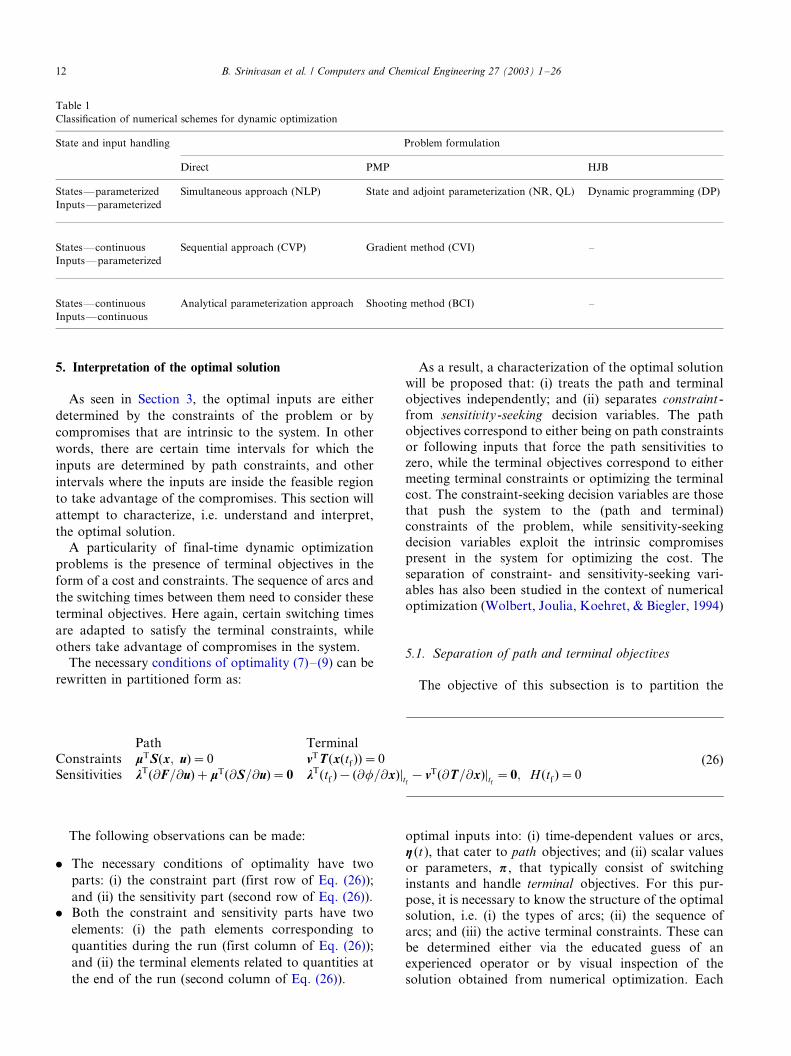
4.4. Classification of numerical optimization schemes

Table 1 classifies the different numerical schemesavailable for solving dynamic optimization problems

according to the underlying problem formulation and

the level of parameterization. Typically, the problem is

easiest to solve when both the states and the inputs are

parameterized (first row in Table 1). When integration

of the system equations is used, parameterization of the

states can be avoided (second row). When, in addition,

analytical expressions derived from the necessary con-ditions of optimality are used to represent the inputs,

both the states and the inputs are continuous (third

row). The two empty boxes in the table result from the

absence of an analytical solution for the partial differ-

ential equation (10)�/(12) of the HJB formulation.

The sequential and simultaneous direct optimization

approaches are by far the methods of choice. Their only

disadvantage is that the input parameterization is oftenchosen arbitrarily by the user. Note that the efficiency of

the approach and the accuracy of the solution depend

crucially on the way the inputs are parameterized.

Though the analytical parameterization approach can

be used to alleviate this difficulty, it becomes arduous

for large size problems. On the other hand, the

numerical methods based on PMP are often numeri-

cally ill conditioned. Though dynamic programming iscomputationally expensive, it is preferred in certain

scenarios due to the fact that the time needed for

optimization can be predetermined.

B. Srinivasan et al. / Computers and Chemical Engineering 27 (2003) 1�/26 11

5. Interpretation of the optimal solution

As seen in Section 3, the optimal inputs are either

determined by the constraints of the problem or by

compromises that are intrinsic to the system. In other

words, there are certain time intervals for which the

inputs are determined by path constraints, and other

intervals where the inputs are inside the feasible region

to take advantage of the compromises. This section will

attempt to characterize, i.e. understand and interpret,

the optimal solution.

A particularity of final-time dynamic optimization

problems is the presence of terminal objectives in the

form of a cost and constraints. The sequence of arcs and

the switching times between them need to consider these

terminal objectives. Here again, certain switching times

are adapted to satisfy the terminal constraints, while

others take advantage of compromises in the system.

The necessary conditions of optimality (7)�/(9) can be

rewritten in partitioned form as:

The following observations can be made:

. The necessary conditions of optimality have two

parts: (i) the constraint part (first row of Eq. (26));

and (ii) the sensitivity part (second row of Eq. (26)).

. Both the constraint and sensitivity parts have two

elements: (i) the path elements corresponding to

quantities during the run (first column of Eq. (26));

and (ii) the terminal elements related to quantities at

the end of the run (second column of Eq. (26)).

As a result, a characterization of the optimal solution

will be proposed that: (i) treats the path and terminalobjectives independently; and (ii) separates constraint-

from sensitivity -seeking decision variables. The path

objectives correspond to either being on path constraints

or following inputs that force the path sensitivities to

zero, while the terminal objectives correspond to either

meeting terminal constraints or optimizing the terminal

cost. The constraint-seeking decision variables are those

that push the system to the (path and terminal)constraints of the problem, while sensitivity-seeking

decision variables exploit the intrinsic compromises

present in the system for optimizing the cost. The

separation of constraint- and sensitivity-seeking vari-

ables has also been studied in the context of numerical

optimization (Wolbert, Joulia, Koehret, & Biegler, 1994)

5.1. Separation of path and terminal objectives

The objective of this subsection is to partition the

optimal inputs into: (i) time-dependent values or arcs,

h (t), that cater to path objectives; and (ii) scalar values

or parameters, p , that typically consist of switching

instants and handle terminal objectives. For this pur-

pose, it is necessary to know the structure of the optimal

solution, i.e. (i) the types of arcs; (ii) the sequence of

arcs; and (iii) the active terminal constraints. These can

be determined either via the educated guess of an

experienced operator or by visual inspection of the

solution obtained from numerical optimization. Each

Table 1

Classification of numerical schemes for dynamic optimization

State and input handling Problem formulation

Direct PMP HJB

States*/parameterized Simultaneous approach (NLP) State and adjoint parameterization (NR, QL) Dynamic programming (DP)

Inputs*/parameterized

States*/continuous Sequential approach (CVP) Gradient method (CVI) �/

Inputs*/parameterized

States*/continuous Analytical parameterization approach Shooting method (BCI) �/

Inputs*/continuous

Path Terminal

Constraints mTS(x; u)�0 nTT(x(tf ))�0

Sensitivities lT(@F=@u)�mT(@S=@u)�0 lT(tf )�(@f=@x)½tf�nT(@T=@x)½tf

�0; H(tf )�0(26)

B. Srinivasan et al. / Computers and Chemical Engineering 27 (2003) 1�/2612

interval is tagged according to the type it could

represent. The analytical expressions for the inputs can

be used for verification but are typically not needed

here.

5.1.1. Meeting path objectives

Path objectives correspond to tracking the active path

constraints and forcing the path sensitivities to zero.

These objectives are achieved through adjustment of the

inputs in the various arcs h (t ) with the help of

appropriate controllers, as will be discussed in thecompanion paper (Srinivasan et al., 2002). Also, among

the switching instants, a few correspond to reaching the

path constraints in minimum time. Thus, these switching

instants are also considered as a part of h (t). The effect

of any deviation in these switching instants will be

corrected by the controllers that keep the corresponding

path objectives active.

5.1.2. Meeting terminal objectives

Upon meeting the path objectives, the optimal inputs

still have residual degrees of freedom that will be used to

meet the terminal objectives, i.e. satisfying terminal

constraints and optimizing the terminal cost. These

input parameters p include certain switching times and

additional decision variables (e.g. the initial conditionsof the inputs as described in Section 3.2).

Upon meeting the path objectives, the optimization

problem reduces to that of minimizing a terminal cost

subject to terminal constraints only . Let the inputs be

represented by u(p , x , t). Then, the optimization pro-

blem (1)�/(3) can be rewritten as:

minp

J�f(x(tf )); (27)

s:t: x�F(x; u(p; x; t)); x(0)�x0; (28)

T(x(tf ))50: (29)

The necessary conditions of optimality for Eqs. (27)�/

(29) are:

nTT(x(tf ))�0 and@f

@p�nT @T

@p�0: (30)

Let t be the number of active terminal constraints.

The number of decision variables arising from the

aforementioned input parameterization, np , needs tosatisfy np] t in order to be able to meet all the active

terminal constraints. Note that np is finite.

5.2. Separation of constraint- and sensitivity-seeking

decision variables

This subsection deals with the separation of thedecision variables according to the nature of the

objectives (constraints vs. sensitivities ). This separation

should be done for both h (t) and p .

5.2.1. Separation of constraint- and sensitivity-seeking

input directions h(t)

In each interval, some of the path constraints may be

active. If there are active path constraints, the inputs or

combinations of inputs that push the system to the path

constraints can be separated from those combinations

that have no effect on meeting the path constraints. Let

z be the number of active path constraints in a given

interval. Clearly, z5m: In the single input case, and in

the extreme cases z�0 and zm; this problem of separa-

tion does not arise. In the other cases, the idea is to use a

transformation, h(t)T 0 [h(t)Th(t)T]; such that h(t) is a

z/-dimensional vector that has a handle on meeting the

path constraints and h(t) is a vector of dimension (m�z) that does not affect the path constraints, but the

sensitivities instead. Thus, h(t) are referred to as the

constraint-seeking input directions, and h(t) as the

sensitivity-seeking input directions.

Let S(x; u) denote the active constraints and m the

corresponding Lagrange multipliers. Let rj be the

relative degree of the constraint Sj(x; u)�0 with respect

to the input that is determined from it. The directions

h(t) and h(t) can be computed using the matrix GS �[f(@=@u)(dr1 S1=dtr1 )g f(@=@u)(dr2 S2=dtr2 )g � � �]T : The

singular value decomposition gives GS�USSSVTS ;

where US has dimension z� z; SS has dimension z�m and VS has dimension m �/m . The matrices US , SS ,

and VS can be partitioned into:

US � [US US]; SS �SS 0

0 0

� ; VS � [VS VS]; (31)

where US and VS correspond to the first z columns of

their respective matrices and US and VS to the remaining

columns. SS is the z� z submatrix of SS . Due to the

structure of SS , GS�USSSVT

S : VS is of dimension m�(m� z) and corresponds to the input directions that do

not affect the constraints. Thus, the constraint- and

sensitivity-seeking directions are defined as: h(t)�V

T

Sh(t) and h(t)�VT

Sh(t): Note that h(t) is a combination

of all inputs that have the same relative degree with

respect to the active constraints S: The directions h(t)

are orthogonal to the directions h(t): Also, for the

sensitivity-seeking input directions, this construction

guarantees that the vector (@=@h)(dkSj=dtk)�0 for

k�/0, 1, . . ., rj . The transformation hT 0 [hT hT] is, in

general, state dependent and can be obtained analyti-

cally if piecewise analytical expressions for the optimal

inputs are available (see Section 3). Otherwise, a

numerical analysis is necessary to obtain this transfor-

mation.With the proposed transformation, the necessary

conditions of optimality for the path objectives are:

B. Srinivasan et al. / Computers and Chemical Engineering 27 (2003) 1�/26 13

S�0;@H

@h�lT @F

@h�0;

@H

@h�lT @F

@h�mT @S

@h�0:

(32)

Thus, the optimal values along the constraint-seeking

directions are determined by the active path constraints

S�0; whilst the optimal values along the sensitivity-

seeking directions are determined from the sensitivity

conditions lT(@F=@h)�0: The third condition in Eq.

(32) determines the value of m: In fact, the advantage of

separating the constraint-seeking from the sensitivity-

seeking input directions is that the necessary conditionsof optimality can be derived without the knowledge of

the Lagrange multiplier m:/

5.2.2. Separation of constraint- and sensitivity-seeking

input parameters p

In the input parameter vector p , there are elements

whose variations affect the active terminal constraints,

T; and others that do not. The idea is then to separate

the two using a transformation, pT 0 [pT pT]; such that

p is a t/-dimensional vector and p is of dimension (np�t): Similar to the classification of the input directions, p

are referred to as the constraint-seeking input para-

meters (with a handle on meeting terminal constraints)

and p as the sensitivity-seeking input parameters (which

are of no help in meeting terminal constraints but will

affect the sensitivities).

Similar to the input directions, the constraint- and

sensitivity-seeking input parameters can be obtainedusing the matrix GT �@T=@p: The singular value

decomposition gives GT �UTST VTT ; where UT has

dimension t� t; ST has dimension t�np and VT has

dimension np�/np . The matrices UT , ST , and VT can be

partitioned into:

UT � [UT UT ]; ST �ST 0

0 0

� ; VT � [VT ; VT ]; (33)

where UT and VT correspond to the first t columns of

their respective matrices and UT and VT to the remain-

ing columns. The constraint- and sensitivity-seeking

parameters can be defined as: p�VT

Tp and p�VT

Tp:This construction guarantees @T=@p�0: Since analy-

tical expressions for @T=@p are not available in most

cases, this transformation is computed numerically.

Though this transformation is in general nonlinear, a

linear approximation can always be found in the

neighborhood of the optimum. This approach was

used in Francois, Srinivasan, and Bonvin (2002) for

the run-to-run optimization of batch emulsion polymer-ization.

Using this transformation, the necessary conditions of

optimality (30) can be rewritten as:

T�0;@f

@p�0;

@f

@p� nT @T

@p�0: (34)

Thus, the active constraints T�0 determine the optimal

values of the constraint-seeking input parameters, whilst

the optimal values of the sensitivity-seeking input

parameters are determined from the sensitivity condi-tions @f=@p�0: The Lagrange multipliers n are calcu-

lated from (@f=@p)� nT(@T=@p)�0:/

5.3. Reasons for interpreting the optimal solution

The interpretation of the optimal solution described

in this section has several advantages that will be

addressed next.

5.3.1. Physical insight

The practitioner likes to be able to relate the variousarcs forming the optimal solution to the physics of his

problem, i.e. the cost to be optimized and the path and

terminal constraints. This knowledge is key towards the

acceptability of the resulting optimal solution in indus-

try.

5.3.2. Numerical efficiency

The efficiency of numerical methods for solving

dynamic optimization problems characterized by adiscontinuous solution depends strongly on the para-

meterization of the inputs. Thus, any parametrization

that is close to the physics of the problem will tend to be

fairly parsimonious and adapted to the problem at

hand. This advantage is most important for the class of

problems where the solution is determined by the

constraints, a category, that encompasses most batch

processes.

5.3.3. Simplified necessary conditions of optimality

With the introduction of S; T; h; h; p and p; the

necessary conditions of optimality reduce to:

Path Terminal

Constraints S(x; u)�0 T(x(tf ))�0

Sensitivities lT(@F=@h)�0 @f=@p�0

(35)

The optimal values along the constraint-seeking direc-

tions, h�(t); are determined by the active path con-

straints S�0; whilst h�(t) are determined from the

sensitivity conditions lT(@F=@h)�0: On the other hand,

the active terminal constraints T�0 determine the

optimal values of the constraint-seeking parameters,

p�; whilst p� are determined from the sensitivity

conditions @f=@p�0: This idea can be used to incor-porate measurements into the optimization framework

so as to combat uncertainty, which will be the subject of

the companion paper (Srinivasan et al., 2002).

B. Srinivasan et al. / Computers and Chemical Engineering 27 (2003) 1�/2614

5.3.4. Variations in cost

Though the necessary conditions of optimality have

four parts as in Eq. (35), each part has a different effect

on the cost. Often, active constraints have a much largerinfluence on the cost than sensitivities do. Thus,

separating constraint- and sensitivity-seeking decision

variables reveals where most of the optimization poten-

tial lies.

The Lagrange multipliers m and n capture the

deviations in cost resulting from the path and terminal

constraints not being active so that, to a first-order

approximation, dJ�ftf

0mT dS dt�nT dT: On the other

hand, if the inputs are inside the feasible region, the

first-order approximation of the cost deviation is zero,

dJ�/(HuSu)�/0, since by definition Hu �/0. Thus, the

loss in performance due to non-optimal inputs is often

less important in a sensitivity-seeking arc than in a

constraint-determined arc. Thus, when implementing an

optimal control policy, care should be taken to keep the

constraints active since this often corresponds to a largegain in performance.

The second-order approximation of the deviation in

performance gives dJ�/(1/2)duTHuudu . If Huu"/0, the

loss could still be significant. However, if Huu�/0, i.e.

for an order of singularity s�/0, then small deviations

of u from the optimal trajectory will result in negligibly

small loss in cost. This negligible effect of input

variations on the cost can also be attributed to the lossof state controllability.

6. Examples

This section presents the optimal solution for several

qualitatively different examples. The emphasis will be on

characterizing the optimal solution by determining those

parts of the optimal solution that push the systemtowards constraints and those parts that seek to reduce

the sensitivities. Also, a clear distinction will be made

between path and terminal objectives. The reason for

choosing four examples (instead of only one) is to

illustrate the various features that an optimal solution

might exhibit. These features are indicated in Table 2.

In every example, the following approach is used: (i) a

numerical solution is first obtained using the direct

sequential method and piecewise-constant parameteriza-

tion of the input; (ii) the different arcs in the solution are

interpreted in terms of satisfying path and terminal

objectives; (iii) with the knowledge of the sequence ofarcs, the analytical parameterization approach is used to

get an exact solution. This last step is not always

necessary, and may not even be appropriate for large

problems. Nevertheless, the analytical expressions are

provided for all examples here since they provide

valuable insight into the solution.

In the sequel, the subscripts ( �/)des, ( �/)min, ( �/)max, ( �/)o,

and ( �/)f represent desired, minimum, maximum, initial,and final values, respectively. usens will be used to

represent a sensitivity-seeking input inside the feasible

region, and upath an input that keeps a path constraint

active.

6.1. Isothermal semi-batch reactor with a safety

constraint (Ubrich et al., 1999)

6.1.1. Description of the reaction system

. Reaction: A�/B 0/C .

. Conditions: Semi-batch, exothermic, isothermal.

. Objective: Minimize the time needed to produce a

given amount of C .

. Manipulated variable: Feed rate of B .

. Constraints: Input bounds; constraint on the max-imum temperature reached under cooling failure;

constraint on the maximum volume.

. Comments: In the case of a cooling failure, the system

becomes adiabatic. The best strategy is to immedi-

ately stop the feed. Yet, due to the presence of

unreacted components in the reactor, the reaction

goes on. Thus, chemical heat will be released, which

causes an increase in temperature. The maximumattainable temperature under cooling failure is given

by:

Tcf (t)�T(t)�min(cA(t); cB(t))(�DH)

rcp

; (36)

where the variables and parameters are described in

Section 6.1.2, and the term min(cA , cB ) serves to

calculate the maximum extent of reaction that could

Table 2

Features present in the various examples

# Example Path con-

straints

Terminal con-

straints

Sensitivity-seeking

arc

Number of in-

puts

Terminal

time

1 Reactor with a safety constraint Yes Yes No 1 Free

2 Bioreactor with inhibition and a biomass constraint Yes No Yes 1 Fixed

3 Reactor with parallel reactions and selectivity con-

straints

No Yes Yes 1 Fixed

4 Non-isothermal reactor with series reactions and a heat

removal constraint

Yes Yes Yes 2 Fixed

B. Srinivasan et al. / Computers and Chemical Engineering 27 (2003) 1�/26 15

occur following the failure.Without any constraints,

optimal operation would simply consist of adding all

the available B at initial time (i.e. batch operation).

However, because of the safety constraint, the feedingof B has to account for the possible cooling failure.

Once the volume constraint is attained, the feed rate

is set to zero.

6.1.2. Problem formulation

6.1.2.1. Variables and parameters. cX , concentration of

species X ; nX , number of moles of species X ; V , reactor

volume; u , feed rate of B ; cB in, inlet concentration of B ;

k , kinetic parameter; T , reactor temperature; Tcf,

temperature under cooling failure; DH , reaction en-

thalpy; r , density; and cp, heat capacity.

6.1.2.2. Model equations.

cA��kcAcB�u

VcA cA(0)�cAo; (37)

cB��kcAcB�u

V(cBin�cB) cB(0)�cBo; (38)

V �u V (0)�Vo: (39)

The concentration of C is given by:

cC �cAoVo � cCoVo � cAV

V: (40)

The numerical values are given in Table 3.

6.1.2.3. Model reduction. The dynamic model (37)�/(39)

can be reduced since the three differential equations are

linearly dependent, as shown next. The balance equa-

tions for various species and total mass read:

nA��kcAcBV nA(0)�nAo; (41)

nB��kcAcBV�cBinu nB(0)�nBo; (42)

V �u; V (0)�Vo: (43)

Eq. (42) can be expressed in terms of Eqs. (41) and (43):

nB� nA�cBinV [d

dt(nB�nA�VcBin)�0; (44)

indicating that I�/nB�/nA�/VcB in�/V (cB�/cA�/cB in) is

a reaction invariant (Srinivasan, Amrhein, & Bonvin,

1998). Integration of Eq. (44) from 0 to t allows

expressing cB in terms of other states and initial

conditions:

cB�(cBo � cAo � cBin)Vo � (cA � cBin)V

V: (45)

6.1.2.4. Optimization problem.

mintf ;u(t)

J�tf ;

s:t: (36); (40); (41); (43); (45)

umin5u(t)5umax;

Tcf (t)5Tmax;

V (tf )5Vmax;

nC(tf )]nCdes: (46)

6.1.2.5. Specific choice of experimental conditions. Let

the experimental conditions be such that the number of

moles of B that can be added is less than the initial

number of moles of A , then cB(t)5/cA(t). Since

isothermal conditions are chosen, the condition

Tcf(t)5/Tmax implies cB(t)5/cB max, with cB max�/

rcp(Tmax�/T )/(�/DH ). Furthermore, the initial condi-tions correspond to having as much B as possible, i.e.

cB o�/cB max�/0.63 mol/l.

6.1.3. Optimal solution

The optimal input and the corresponding evolution of

the concentrations of A , B and C obtained numerically

are given in Fig. 1. The optimal input consists of the two

arcs upath and umin:

. Since the initial conditions verify cB o�/cB max, upath is

applied to keep cB �/cB max, i.e. Tcf�/Tmax.

. Once V�/Vmax is attained, the input is set to umin�/0.

. Once nC �/nC des is attained, the batch is stopped so asto minimize the final time.

For the numerical values provided in Table 3, the

minimal time J��tf��19:80 h is obtained with the

switching time ts�/11.44 h.

Table 3

Model parameters, operating bounds and initial conditions for

Example 1

k 0.0482 l/mol h

T 70 8CDH �60 000 J/mol

r 900 g/l

cp 4.2 J/gK

cB in 2 mol/l

umin 0 l/h

umax 0.1 l/h

Tmax 80 8CVmax 1 l

nC des 0.6 mol

cA o 2 mol/l

cB o 0.63 mol/l

Vo 0.7 l

B. Srinivasan et al. / Computers and Chemical Engineering 27 (2003) 1�/2616

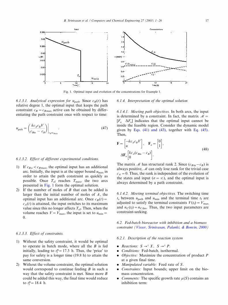
6.1.3.1. Analytical expression for upath. Since cB (t ) has

relative degree 1, the optimal input that keeps the path

constraint cB �/cB max active can be obtained by differ-

entiating the path constraint once with respect to time:

upath��

kcAcBV

cBin � cB

�jcB�cBmax

: (47)

6.1.3.2. Effect of different experimental conditions.

1) If cB oB/cB max, the optimal input has an additionalarc. Initially, the input is at the upper bound umax in

order to attain the path constraint as quickly as

possible. Once Tcf reaches Tmax, the two arcs

presented in Fig. 1 form the optimal solution.

2) If the number of moles of B that can be added is

larger than the initial number of moles of A , the

optimal input has an additional arc. Once cB (t)�/

cA (t) is attained, the input switches to its maximumvalue since this no longer affects Tcf. Then, when the

volume reaches V�/Vmax, the input is set to umin�/

0.

6.1.3.3. Effect of constraints.

1) Without the safety constraint, it would be optimal

to operate in batch mode, where all the B is fed

initially, leading to tf��17:3 h: Thus, the ‘price’ to

pay for safety is a longer time (19.8 h) to attain the

same conversion.

2) Without the volume constraint, the optimal solution

would correspond to continue feeding B in such away that the safety constraint is met. Since more B

could be added this way, the final time would reduce

to tf��18:4 h:/

6.1.4. Interpretation of the optimal solution

6.1.4.1. Meeting path objectives. In both arcs, the input

is determined by a constraint. In fact, the matrix M�[Fu DFu] indicates that the optimal input cannot beinside the feasible region. Consider the dynamic model

given by Eqs. (41) and (43), together with Eq. (45).

Then,

F��kcAcBV

u

� ; Fu�

0

1

� ;

DFu

kcA(cBin�cB)

0

� :

(48)

The matrix M has structural rank 2. Since (cB in�/cB) isalways positive, M can only lose rank for the trivial case

cA �/0. Thus, the rank is independent of the evolution of

the states and input (s�/�), and the optimal input is

always determined by a path constraint.

6.1.4.2. Meeting terminal objectives. The switching timets between upath and umin and the terminal time tf are

adjusted to satisfy the terminal constraints V (tf)�/Vmax

and nC (tf)�/nC des. Thus, the two input parameters are

constraint-seeking.

6.2. Fed-batch bioreactor with inhibition and a biomass

constraint (Visser, Srinivasan, Palanki, & Bonvin, 2000)

6.2.1. Description of the reaction system

. Reactions: S 0x X ; S 0x P:/

. Conditions: Fed-batch, isothermal.

. Objective: Maximize the concentration of product P

at a given final time.

. Manipulated variable: Feed rate of S .

. Constraints: Input bounds; upper limit on the bio-mass concentration.

. Comments: The specific growth rate m(S ) contains an

inhibition term:

Fig. 1. Optimal input and evolution of the concentrations for Example 1.

B. Srinivasan et al. / Computers and Chemical Engineering 27 (2003) 1�/26 17

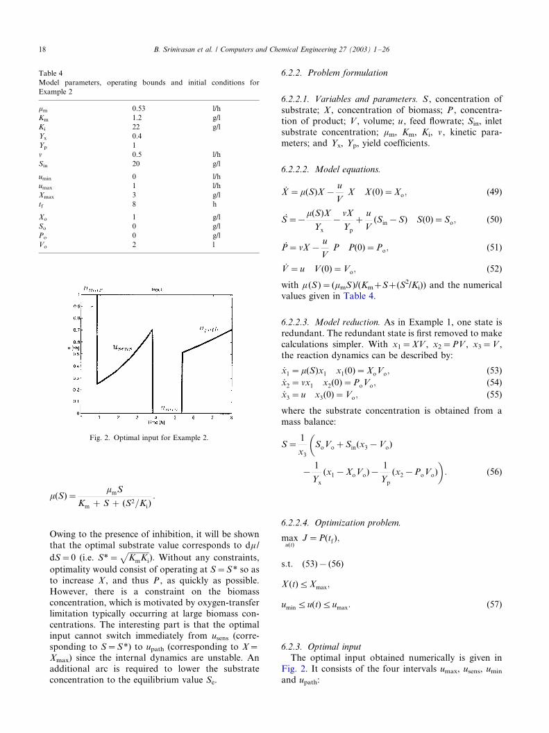
m(S)�mmS

Km � S � (S2=Ki):

Owing to the presence of inhibition, it will be shown

that the optimal substrate value corresponds to dm /

dS�/0 (i.e. S��ffiffiffiffiffiffiffiffiffiffiffiKmKi

p): Without any constraints,

optimality would consist of operating at S�/S� so as

to increase X , and thus P , as quickly as possible.

However, there is a constraint on the biomass

concentration, which is motivated by oxygen-transfer

limitation typically occurring at large biomass con-

centrations. The interesting part is that the optimal

input cannot switch immediately from usens (corre-

sponding to S�/S�) to upath (corresponding to X�/

Xmax) since the internal dynamics are unstable. An

additional arc is required to lower the substrate

concentration to the equilibrium value Se.

6.2.2. Problem formulation

6.2.2.1. Variables and parameters. S , concentration of

substrate; X , concentration of biomass; P , concentra-tion of product; V , volume; u , feed flowrate; Sin, inlet

substrate concentration; mm, Km, Ki, n , kinetic para-

meters; and Yx, Yp, yield coefficients.

6.2.2.2. Model equations.

X �m(S)X �u

VX X (0)�Xo; (49)

S��m(S)X

Yx

�nX

Yp

�u

V(Sin�S) S(0)�So; (50)

P�nX �u

VP P(0)�Po; (51)

V �u V (0)�Vo; (52)

with m(S )�/(mmS )/(Km�/S�/(S2/Ki)) and the numericalvalues given in Table 4.

6.2.2.3. Model reduction. As in Example 1, one state is

redundant. The redundant state is first removed to make

calculations simpler. With x1�/XV , x2�/PV , x3�/V ,

the reaction dynamics can be described by:

x1�m(S)x1 x1(0)�XoVo; (53)

x2�nx1 x2(0)�PoVo; (54)

x3�u x3(0)�Vo; (55)

where the substrate concentration is obtained from a

mass balance:

S�1

x3

�SoVo�Sin(x3�Vo)

�1

Yx

(x1�XoVo)�1

Yp

(x2�PoVo)

�: (56)

6.2.2.4. Optimization problem.

maxu(t)

J�P(tf );

s:t: (53)�(56)

X (t)5Xmax;

umin5u(t)5umax: (57)

6.2.3. Optimal input

The optimal input obtained numerically is given in

Fig. 2. It consists of the four intervals umax, usens, umin

and upath:

Table 4

Model parameters, operating bounds and initial conditions for

Example 2

mm 0.53 l/h

Km 1.2 g/l

Ki 22 g/l

Yx 0.4

Yp 1

n 0.5 l/h

Sin 20 g/l

umin 0 l/h

umax 1 l/h

Xmax 3 g/l

tf 8 h

Xo 1 g/l

So 0 g/l

Po 0 g/l

Vo 2 l

Fig. 2. Optimal input for Example 2.

B. Srinivasan et al. / Computers and Chemical Engineering 27 (2003) 1�/2618

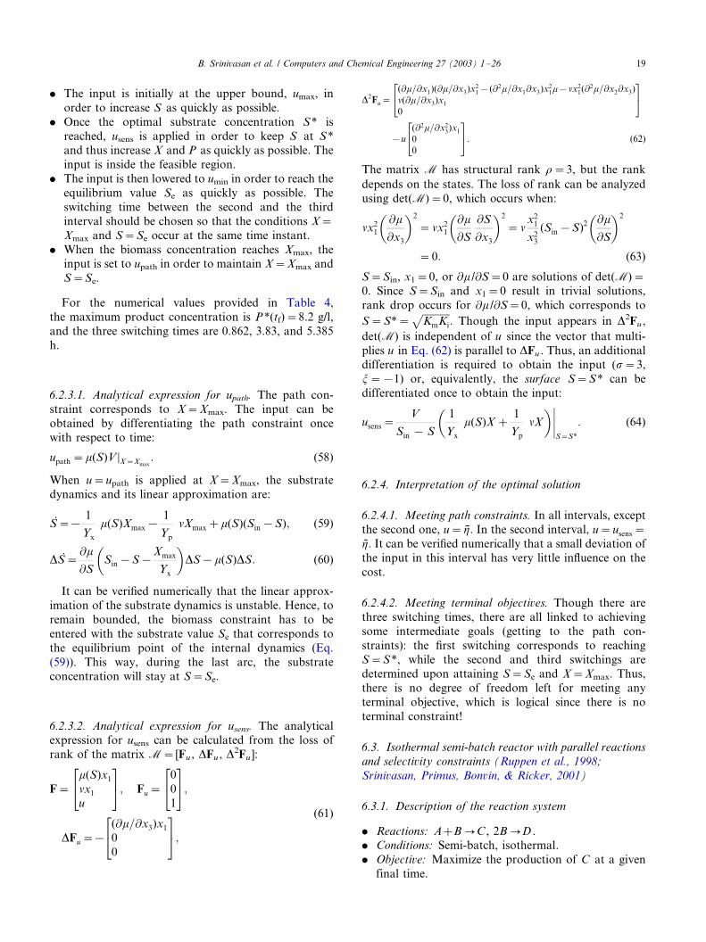
. The input is initially at the upper bound, umax, in

order to increase S as quickly as possible.

. Once the optimal substrate concentration S� is

reached, usens is applied in order to keep S at S�and thus increase X and P as quickly as possible. The

input is inside the feasible region.

. The input is then lowered to umin in order to reach the

equilibrium value Se as quickly as possible. The

switching time between the second and the third

interval should be chosen so that the conditions X�/

Xmax and S�/Se occur at the same time instant.

. When the biomass concentration reaches Xmax, theinput is set to upath in order to maintain X�/Xmax and

S�/Se.

For the numerical values provided in Table 4,

the maximum product concentration is P�(tf)�/8.2 g/l,

and the three switching times are 0.862, 3.83, and 5.385

h.

6.2.3.1. Analytical expression for upath. The path con-

straint corresponds to X�/Xmax. The input can be

obtained by differentiating the path constraint once

with respect to time:

upath�m(S)V ½X�Xmax: (58)

When u�/upath is applied at X�/Xmax, the substrate

dynamics and its linear approximation are:

S��1

Yx

m(S)Xmax�1

Yp

nXmax�m(S)(Sin�S); (59)

DS�@m

@S

�Sin�S�

Xmax

Yx

�DS�m(S)DS: (60)

It can be verified numerically that the linear approx-

imation of the substrate dynamics is unstable. Hence, to

remain bounded, the biomass constraint has to be

entered with the substrate value Se that corresponds to

the equilibrium point of the internal dynamics (Eq.

(59)). This way, during the last arc, the substrate

concentration will stay at S�/Se.

6.2.3.2. Analytical expression for usens. The analyticalexpression for usens can be calculated from the loss of

rank of the matrix M�/[Fu , DFu , D2Fu ]:

F�m(S)x1

nx1

u

24

35; Fu�

0

0

1

24

35;

DFu��(@m=@x3)x1

0

0

24

35;

(61)

D2Fu�(@m=@x1)(@m=@x3)x2

1�(@2m=@x1@x3)x21m�nx2

1(@2m=@x2@x3)

n(@m=@x3)x1

0

24

35

�u(@2m=@x2

3)x1

0

0

24

35: (62)

The matrix M has structural rank r�/3, but the rank

depends on the states. The loss of rank can be analyzed

using det(M)�/0, which occurs when:

nx21

�@m

@x3

�2

�nx21

�@m

@S

@S

@x3

�2

�nx2

1

x23

(Sin�S)2

�@m

@S

�2

�0: (63)

S�/Sin, x1�/0, or @m /@S�/0 are solutions of det(M)�/

0. Since S�/Sin and x1�/0 result in trivial solutions,

rank drop occurs for @m /@S�/0, which corresponds to

S�S��ffiffiffiffiffiffiffiffiffiffiffiKmKi

p: Though the input appears in D2Fu ,

det(M) is independent of u since the vector that multi-

plies u in Eq. (62) is parallel to DFu . Thus, an additionaldifferentiation is required to obtain the input (s�/3,

j�/�/1) or, equivalently, the surface S�/S� can be

differentiated once to obtain the input:

usens�V

Sin � S

�1

Yx

m(S)X �1

Yp

nX

�jS�S�

: (64)

6.2.4. Interpretation of the optimal solution

6.2.4.1. Meeting path constraints. In all intervals, except

the second one, u� h: In the second interval, u�usens�h: It can be verified numerically that a small deviation of

the input in this interval has very little influence on the

cost.

6.2.4.2. Meeting terminal objectives. Though there are

three switching times, there are all linked to achieving

some intermediate goals (getting to the path con-

straints): the first switching corresponds to reachingS�/S�, while the second and third switchings are

determined upon attaining S�/Se and X�/Xmax. Thus,

there is no degree of freedom left for meeting any

terminal objective, which is logical since there is no

terminal constraint!

6.3. Isothermal semi-batch reactor with parallel reactions

and selectivity constraints (Ruppen et al., 1998;

Srinivasan, Primus, Bonvin, & Ricker, 2001)

6.3.1. Description of the reaction system

. Reactions: A�/B 0/C , 2B 0/D .

. Conditions: Semi-batch, isothermal.

. Objective: Maximize the production of C at a given

final time.

B. Srinivasan et al. / Computers and Chemical Engineering 27 (2003) 1�/26 19

. Manipulated variable: Feed rate of B .

. Constraints: Input bounds; constraints on the max-

imum concentrations of B and D at final time.

. Comments: If the second (undesired) reaction wereabsent, it would be optimal to have as large a value of

cB as possible. The optimization potential is created

by the presence of the second reaction, thereby giving

rise to a possible compromise. However, this com-

promise is only present when there is a constraint on

the final amount of D . Note that, in the absence of

constraints, optimal operation would simply consist

of adding all the available B at initial time (i.e. batchoperation). Furthermore, since the amount of B

present in the reactor at final time is limited, the

feed rate of B is turned off towards the end of the

batch.

6.3.2. Problem formulation

6.3.2.1. Variables and parameters. cX , concentration of

species X ; V , reactor volume; u , feed rate of B ; cB in,

inlet concentration of B ; and k1, k2, kinetic parameters.

6.3.2.2. Model equations.

cA��k1cAcB�u

VcA cA(0)�cAo; (65)

cB��k1cAcB�2k2c2B�

u

V(cBin�cB) cB(0)�cBo; (66)

V �u V (0)�Vo; (67)

with

cC �1

V(cAoVo�cAV ); (68)

cD�1

2V((cA�cBin�cB)V�(cAo�cBin�cBo)Vo): (69)

The numerical values are given in Table 5.

6.3.2.3. Optimization problem.

maxu(t)

J�V (tf ) cC(tf );

s:t: (65)�(69)

umin5u(t)5umax;

cB(tf )5cBf;max;

cD(tf )5cDf ;max: (70)

6.3.3. Optimal input

The optimal input obtained numerically is given inFig. 3. It consists of the three intervals umax, usens and

umin:

. The input is initially at the upper bound umax to

increase cB and thus the rate of the desired reaction.

. The input switches to the sensitivity-seeking arc so

that only a limited amount of D is produced.

. The input switches to umin so that cB can meet its

constraint at final time.

For the numerical values provided in Table 5, the

maximum number of moles of C is nC� (tf )�0:43 mol;and the two switching times are tm�/20.25 and ts�/205h.

6.3.3.1. Analytical expression for usens. The analytical

expression for usens can be determined using the matrix

M�/[Fu , DFu , D2Fu ]:

F��k1cAcB

�k1cAcB�2k2c2B

0

24

35� 1

V

�cA

cBin�cB

V

24

35u;

Fu�1

V

�cA

cBin�cB

V

24

35;

Table 5

Model parameters, operating bounds and initial conditions for

Example 3

k1 0.053 l/mol min

k2 0.128 l/mol min

cB in 5 mol/l

umin 0 l/min

umax 0.001 l/min

cB f,max 0.025 mol/l

cD f,max 0.15 mol/l

cA o 0.72 mol/l

cB o 0.05 mol/l

Vo 1 l

tf 250 min

Fig. 3. Optimal input for Example 3.

B. Srinivasan et al. / Computers and Chemical Engineering 27 (2003) 1�/2620

DFu�1

V

k1cA(cBin�cB)

k1cA(cBin�cB)�2k2cB(2cBin�cB)

0

24

35;

D2Fu�cBin

V

k21c2

A�4k1k2cAcB

k21c2

A�4k1k2cAcB�8k22c2

B

0

24

35�2(cBin�cB)

� u

V 2

k1cA

k1cA�2k2(cBin�cB)0

24

35:

The matrix M has structural rank r�/3. However, since

the rank depends on the states and input, it may be

possible to reduce it by an appropriate combination of

states and input, i.e. usens�/u(x ). The combination of xand u for which the rank of M drops can be computed

from det(M)�/0. The input appears in D2Fu , which

indicates that the order of singularity is s�/2. Since j�/

0, a static feedback for the optimal input can becomputed from det(M)�/0:

usens�cBincBV (k1cA(2cBin � cB) � 4k2cBcBin)

2(cBin � cB): (71)

6.3.4. Interpretation of the optimal solution

6.3.4.1. Meeting path objectives. In the first and thirdintervals, u� h; while u�usens� h in the second one. It

can be verified numerically that a small deviation of the

input in the second interval has very little influence on

the cost.

6.3.4.2. Meeting terminal objectives. The two switchingtimes tm and ts parameterize the solution completely. In

turn, they are determined by the two active terminal

constraints cB (tf)�/cB f,max and cD(tf)�/cD f,max. Thus,

the two input parameters in this example are constraint-

seeking parameters.

Since the second interval is sensitivity-seeking, it is

possible to approximate it by a constant, without

significant loss in performance. Consider the case whereusens(t) is approximated by the scalar value us. Then,

there are three parameters, (tm, ts, and us), to meet the

two terminal constraints and optimize the cost. The gain

matrix GT : p0/T computed in the neighborhood of the

optimal solution, with p�/[tm, ts, us]T and T (x (tf))�/

[cD(tf)�/cD f,max, cB (tf)�/cB f,max]T, is given by:

GT �0:6�10�3 0:5�10�3 1:5�102

1:9�10�5 1:1�10�3 0:2�102

� :

Using singular value decomposition, it can be seen that

p� tm�4:7�10�2 ts�4�10�6 us: Since the contribu-tions from ts and us are negligible, tm essentially acts as

the sensitivity-seeking parameter. It is interesting to note

that tm, which was a constraint-seeking parameter when

usens was not approximated, becomes a sensitivity-

seeking parameter after the approximation. This can

be explained by the fact that the new input parameter us

has a strong effect on the constraints (see the lastcolumn of GT) and becomes the dominant constraint-

seeking parameter.

6.4. Non-isothermal semi-batch reactor with series

reactions and a heat removal constraint

6.4.1. Description of the reaction system

. Reactions: A�/B0/C 0/D .

. Conditions: Semi-batch, exothermic, non-isothermal,

operated in a jacketed reactor such that the reactor

temperature can be adjusted quickly.

. Objective: Maximize the production of C at a given

final time.

. Manipulated variables: Feed rate of B and reactor

temperature.

. Constraints: Bounds on feed rate and reactor tem-perature; constraint on the maximum heat that can

be removed by the cooling system; constraint on the

maximum volume.

. Comments: The reactor temperature is assumed to be

a manipulated variable though, in practice, either the

flowrate or the temperature in the cooling jacket is

manipulated. The heat balance equation for the

reactor is: rcp(VdT /dt )�/qrx�/qin�/qex, where V isthe reactor volume; T , the reactor temperature; r ,

the density; cp, the heat capacity; qrx, the rate of heat

produced by the reactions; qin, the rate of heat

removal associated with the feed of B ; and qex, the

rate of heat removal through the cooling jacket. The

inclusion of the heat balance equation would com-

plicate the analytical expressions without fundamen-

tally changing the types and sequence of arcs presentin the solution. Thus, for simplicity, the heat balance

equation will be neglected. However, to guarantee

meeting the upper bound on qex even in the worst

scenario, it is necessary to limit qrx as follows: qrx5/

max(qex)�/min(qin�/rcp(VdT /dt ))�/qrx,max. Thus, an

upper bound on the heat rate produced by the

reactions, qrx5/qrx,max, is imposed as a constraint.The

consumption of the desired product C by theundesired reaction is reduced by lowering the tem-

perature towards the end of the batch. The compro-

mise between the production and consumption of C

corresponds to a sensitivity-seeking temperature

profile. As far as the feed rate is concerned, it is first

determined by the heat removal constraint and then

by the volume constraint.Without any constraints,

optimal operation would consist of adding all theavailable B at initial time and following a tempera-

ture profile that expresses the compromise between

the production and consumption of C .

B. Srinivasan et al. / Computers and Chemical Engineering 27 (2003) 1�/26 21

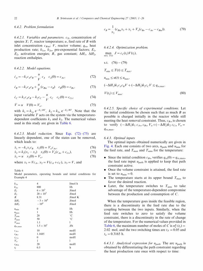
6.4.2. Problem formulation

6.4.2.1. Variables and parameters. cX , concentration ofspecies X ; T , reactor temperature; u , feed rate of B with

inlet concentration cB in; V , reactor volume; qrx, heat

production rate; k1o, k2o, pre-exponential factors; E1,

E2, activation energies; R , gas constant; DH1, DH2,

reaction enthalpies.

6.4.2.2. Model equations.

cA��k1cAcB�u

VcA cA(0)�cAo; (72)

cB��k1cAcB�u

V(cBin�cB) cB(0)�cBo; (73)

cC �k1cAcB�k2cC�u

VcC cC(0)�cCo; (74)

V �u V (0)�Vo; (75)

with k1�k1o e�E1=RT ; k2�k2o e�E2=RT : Note that the

input variable T acts on the system via the temperature-

dependent coefficients k1 and k2. The numerical values

used in this study are given in Table 6.

6.4.2.3. Model reduction. Since Eqs. (72)�/(75) are

linearly dependent, one of the states can be removed,

which leads to:

x1��k1x1cB x1(0)�VocAo; (76)

x2�k2(x1�x2) x2(0)�Vo(cAo�cCo); (77)

x3�u x3(0)�Vo; (78)

where x1�/VcA , x2�/V (cA�/cC ), x3�/V , and

cB�1

x3

(cBinx3�x1�Vo(cBo�cAo�cBin)): (79)

6.4.2.4. Optimization problem.

maxu(t); T(t)

J�cC(tf )V (tf );

s:t: (76)�(79)

Tmin5T(t)5Tmax;

umin5u(t)5umax;

(�DH1)k1cAcBV�(�DH2)k2cCV 5qrx;max;

V (tf )5Vmax: (80)

6.4.2.5. Specific choice of experimental conditions. Let

the initial conditions be chosen such that as much B as

possible is charged initially in the reactor while still

meeting the heat removal constraint. Thus, cB o is chosen

to verify (�/DH1)k1 cA o cB o Vo�/(�/DH2)k2 cC o Vo�/

qrx,max.

6.4.3. Optimal inputs

The optimal inputs obtained numerically are given in

Fig. 4. Each one consists of two arcs, upath and umin for

the feed rate, and Tmax and Tsens for the temperature:

. Since the initial condition cB o verifies qrx(0)�/qrx,max,

the feed rate input upath is applied to keep that path

constraint active.. Once the volume constraint is attained, the feed rate

is set to umin�/0.

. The temperature starts at its upper bound Tmax to

favor the desired reaction.

. Later, the temperature switches to Tsens to take

advantage of the temperature-dependent compromise

between the production and consumption of C .

When the temperature goes inside the feasible region,

there is a discontinuity in the feed rate due to thecoupling between the two inputs. Similarly, when the

feed rate switches to zero to satisfy the volume

constraint, there is a discontinuity in the rate of change

of the temperature. For the numerical values provided in

Table 6, the maximum number of moles of C is nC� (tf )�2:02 mol; and the two switching times are tT �/0.05 and

tu �/0.3165 h.

6.4.3.1. Analytical expression for upath. The arc upath is

obtained by differentiating the path constraint regarding

the heat production rate once with respect to time:

Table 6

Model parameters, operating bounds and initial conditions for

Example 4

k1o 4 l/mol h

k2o 800 l/h

E1 6�103 J/mol

E2 20�103 J/mol

R 8.31 J/mol K

DH1 �3�104 J/mol

DH2 �104 J/mol

umin 0 l/h

umax 1 l/h

Tmin 20 8CTmax 50 8CVmax 1.1 l

qrx,max 1.5�105 J/h

cA o 10 mol/l

cB o 1.1685 mol/l

cC o 0 mol/l

Vo 1 l

cB in 20 mol/l

tf 0.5 h

B. Srinivasan et al. / Computers and Chemical Engineering 27 (2003) 1�/2622

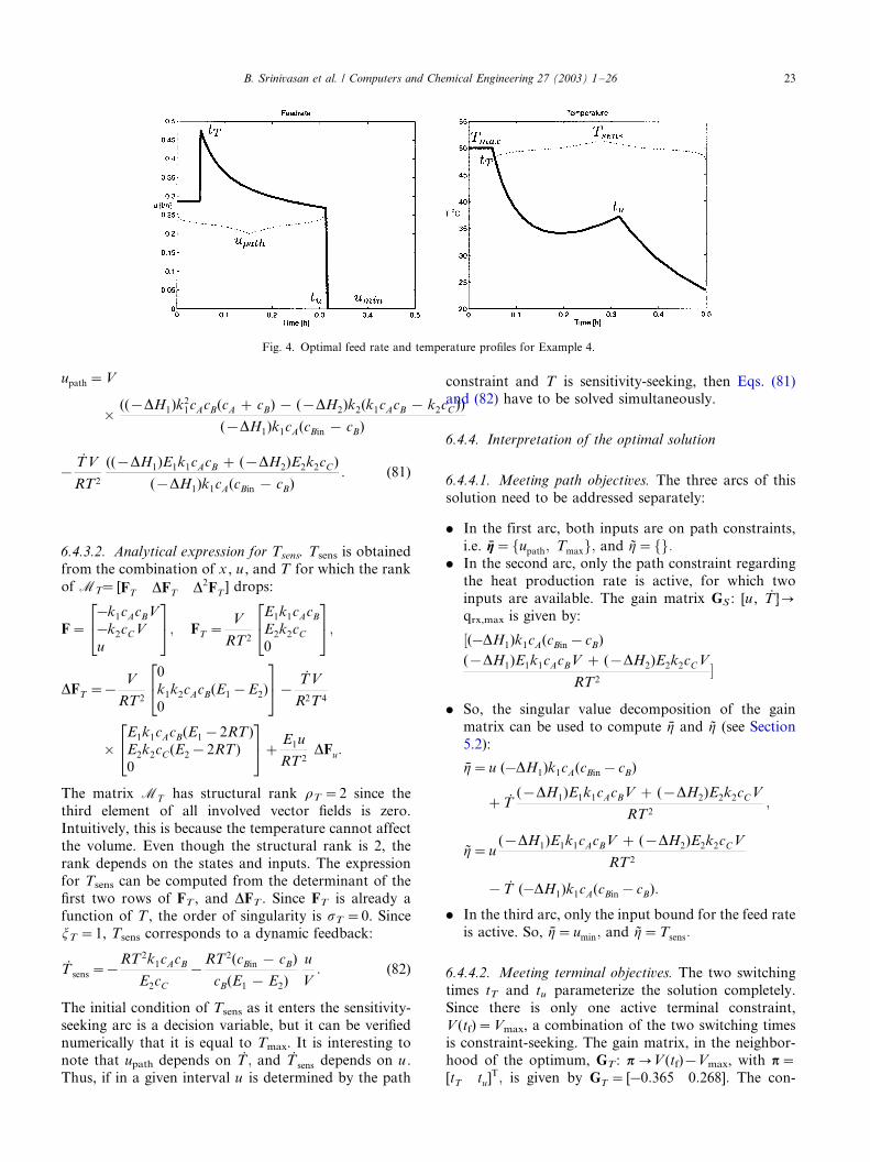
upath�V

� ((�DH1)k21cAcB(cA � cB) � (�DH2)k2(k1cAcB � k2cC))

(�DH1)k1cA(cBin � cB)

�TV

RT2

((�DH1)E1k1cAcB � (�DH2)E2k2cC)

(�DH1)k1cA(cBin � cB): (81)

6.4.3.2. Analytical expression for Tsens. Tsens is obtained

from the combination of x , u , and T for which the rank

of MT/� [FT DFT D2FT] drops:

F��k1cAcBV

�k2cCV

u

24

35; FT �

V

RT2

E1k1cAcB

E2k2cC

0

24

35;

DFT ��V

RT2

0

k1k2cAcB(E1�E2)

0

24

35� TV

R2T4

�E1k1cAcB(E1�2RT)

E2k2cC(E2�2RT)0

24

35� E1u

RT 2DFu:

The matrix MT has structural rank rT �/2 since the

third element of all involved vector fields is zero.

Intuitively, this is because the temperature cannot affect

the volume. Even though the structural rank is 2, the

rank depends on the states and inputs. The expression

for Tsens can be computed from the determinant of the

first two rows of FT , and DFT . Since FT is already a

function of T , the order of singularity is sT �/0. SincejT �/1, Tsens corresponds to a dynamic feedback:

T sens��RT 2k1cAcB

E2cC

�RT2(cBin � cB)

cB(E1 � E2)

u

V: (82)

The initial condition of Tsens as it enters the sensitivity-

seeking arc is a decision variable, but it can be verifiednumerically that it is equal to Tmax. It is interesting to

note that upath depends on T ; and T sens depends on u .

Thus, if in a given interval u is determined by the path

constraint and T is sensitivity-seeking, then Eqs. (81)and (82) have to be solved simultaneously.

6.4.4. Interpretation of the optimal solution

6.4.4.1. Meeting path objectives. The three arcs of this

solution need to be addressed separately:

. In the first arc, both inputs are on path constraints,

i.e. h�fupath; Tmaxg; and h�fg:/. In the second arc, only the path constraint regarding

the heat production rate is active, for which two

inputs are available. The gain matrix GS : [u , T ]/0/

qrx,max is given by:

(�DH1)k1cA(cBin�cB)½(�DH1)E1k1cAcBV � (�DH2)E2k2cCV

RT 2�

. So, the singular value decomposition of the gain

matrix can be used to compute h and h (see Section

5.2):

h�u (�DH1)k1cA(cBin�cB)

�T(�DH1)E1k1cAcBV � (�DH2)E2k2cCV

RT2;

h�u(�DH1)E1k1cAcBV � (�DH2)E2k2cCV

RT2

�T (�DH1)k1cA(cBin�cB):

. In the third arc, only the input bound for the feed rate

is active. So, h�umin; and h�Tsens:/

6.4.4.2. Meeting terminal objectives. The two switching

times tT and tu parameterize the solution completely.

Since there is only one active terminal constraint,

V (tf)�/Vmax, a combination of the two switching timesis constraint-seeking. The gain matrix, in the neighbor-

hood of the optimum, GT : p0/V (tf)�/Vmax, with p�[tT tu]T; is given by GT � [�0:365 0:268]: The con-

Fig. 4. Optimal feed rate and temperature profiles for Example 4.

B. Srinivasan et al. / Computers and Chemical Engineering 27 (2003) 1�/26 23

straint-seeking parameter is p�0:365tT �0:268tu; while

the sensitivity-seeking parameter is given by

p�0:268tT �0:365tu:/

7. Conclusions

This paper first presented an overview of the analy-

tical and numerical techniques that are available in the

literature to solve dynamic optimization problems with

a special emphasis on classification. For the analytical

techniques, the classification was based on whether or

not the adjoint variables are used. For the numerical

techniques, the classification was based on the problem

formulation and the type of parameterization used.

Most techniques proposed in the literature for the

optimization of dynamic processes take a black-box

approach. In contrast, this paper emphasizes the solution

structure that arises from interplay between manipu-

lated variables, cost and constraints. Certain intervals of

the optimal solution are linked to path constraints, while

others are shown to be inside the feasible region. Thus,

the optimal inputs can be presented in terms of

constraint- and sensitivity-seeking intervals. In addition,

some of the switching times between the various

intervals can also be interpreted as constraint- and

sensitivity-seeking parameters that are selected for meet-

ing terminal constraints or optimizing the terminal-time

objective function. A series of examples are provided to

illustrate these concepts.

The main application of the characterization pre-

sented in this paper is linked to the design of measure-

ment-based optimization strategies. Handling

uncertainty in the context of optimization is a very

important issue, especially in the presence of constraints

on quality and safety. Most optimization techniques are

model -based , whilst accurate models of industrial batch

processes are rarely available. With the advent of recent

developments in sensor technology, measurement -based

optimization strategies could be used to cope with

uncertainty. These strategies, which constitute the focus

of the companion paper (Srinivasan et al., 2002), are

based on the characterization presented in this work.

Acknowledgements

The authors would like to thank the anonymous

reviewer, whose helpful comments have been used to

improve this paper, and the Swiss National Science

Foundation, grant number 21-46922.96, for supporting

this research work.

References

Abel, O., Helbig, A., Marquardt, W., Zwick, H., & Daszkowski, T.

(2000). Productivity optimization of an industrial semi-batch

polymerization reactor under safety constraints. Journal of Process

Control 10 (4), 351�/362.

Allgor, R. J., Barrera, M. D., Barton, P. I., & Evans, L. B. (1996).

Optimal batch process development. Computers and Chemical

Engineering 20 (6�/7), 885�/896.

Barrera, M. D., & Evans, L. B. (1989). Optimal design and operation

of batch processes. Chemical Engineering Communication 82 , 45�/

66.

Basu, P. K. (1998). Pharmaceutical process development is different!

Chemical Engineering Progress 94 (9), 75�/82.

Baumann, T. (1998). Infinite-order singularity in terminal-cost optimal

control: application to robotic manipulators . PhD thesis 1778.

Lausanne, Switzerland: Swiss Federal Institute of Technology

(EPFL).

Bell, M. L., Limebeer, D. J. N., & Sargent, R. W. H. (1996). Robust

receding horizon optimal control. Computers and Chemical En-

gineering 20 , S781�/S786.

Bellman, R. E. (1957). Dynamic programming . Princeton University

Press.

Benthack, C. (1997). Feedback -based optimization of a class of

constrained nonlinear systems: application to a biofilter . PhD thesis

1717. Lausanne, Switzerland: Swiss Federal Institute of Technol-

ogy (EPFL).

Biegler, L. T. (1984). Solution of dynamic optimization problems by

successive quadratic programming and orthogonal collocation.

Computers and Chemical Engineering 8 , 243�/248.

Biegler, L. T., Cervantes, A. M., & Wachter, M. A. (2002). Advances

in simultaneous strategies for dynamic process optimization.

Chemical Engineering Science 57 , 575�/593.

Bock, H. G., & Platt, K. J. (1984). A multiple shooting algorithm for

direct solution of optimal control problems. In 9th IFAC world

congress (pp. 242�/247). Budapest.

Bojkov, B., & Luus, R. (1994). Time-optimal control by iterative

dynamic programming. Industrial and Engineering Chemistry

Research 33 , 1486�/1492.

Bonvin, D. (1998). Optimal operation of batch reactors*/a personal

view. Journal of Process Control 8 (5�/6), 355�/368.

Bonvin, D., Srinivasan, B., & Ruppen, D. (2001). Dynamic optimiza-

tion in the batch chemical industry. Proceedings of the CPC-VI

Conference. American Institute of Chemical Engineers, Symposium

Series 326 (98), 255�/273.

Bryson, A. E. (1999). Dynamic optimization . Menlo Park, CA:

Addison-Wesley.

Bryson, A. E., & Ho, Y. C. (1975). Applied optimal control .

Washington DC: Hemisphere.

Cervantes, A., & Biegler, L. T. (1998). Large-scale DAE optimization

using a simultaneous NLP formulation. American Institute of

Chemical Engineers Journal 44 (5), 1038�/1050.

Chen, S. A., & Jeng, W. F. (1978). Minimum end time policies for

batchwise radical chain polymerization. Chemical Engineering

Science 33 , 735.

Chu, W. B. (1987). Modeling, optimization and computer control of the

Cephalosporin C fermentation process. PhD thesis. New Brunswick,

New Jersey, USA: Rutgers, The State University of New Jersey.

Cuthrell, J. E., & Biegler, L. T. (1987). On the optimization of

differential-algebraic process systems. American Institute of Che-

mical Engineers Journal 33 , 1257�/1270.

Cuthrell, J. E., & Biegler, L. T. (1989). Simultaneous optimization

methods for batch reactor control profiles. Computers and Chemi-

cal Engineering 13 , 49�/62.

Diwekar, U. M. (1995). Batch distillation: simulation, optimal design

and control . Washington: Taylor and Francis.

B. Srinivasan et al. / Computers and Chemical Engineering 27 (2003) 1�/2624

Eaton, J. W., & Rawlings, J. B. (1990). Feedback control of nonlinear

processes using on-line optimization techniques. Computers and

Chemical Engineering 14 , 469�/479.

Edgar, T. F., & Himmelblau, D. M. (1988). Optimization of chemical

processes . New York: McGraw-Hill.

Fikar, M., Latifi, M. A., Fournier, F., & Creff, Y. (1998). Control-

vector parameterization versus iterative dynamic programming in

dynamic optimization of a distillation column. Computers and

Chemical Engineering 22 , S625�/S628.

Francois, G., Srinivasan, B., & Bonvin, D. (2002). Run-to-run

optimization of batch emulsion polymerization. In 15th IFAC

world congress (Vol. T-Mo-M11). Barcelona, Spain.

Friedrich, M., & Perne, R. (1995). Design and control of batch

reactors: an industrial viewpoint. Computers and Chemical En-

gineering 19 , S357�/S368.

Furlonge, H. I., Pantelides, C. C., & Sorensen, E. (1999). Optimal

operation of multivessel batch distillation columns. American

Institute of Chemical Engineers Journal 45 (4), 781�/800.

Gill, P. E., Murray, W., & Wright, M. H. (1981). Practical optimiza-

tion . London: Academic Press.

Giritligil, S., Cesur, S., & Kuryel, B. (1998). Overview of planning and

scheduling of batch process operations. In IFAC DYCOPS-5 (pp.

461�/466). Corfu, Greece.

Goh, C. J., & Teo, K. L. (1988). Control parameterization: a unified

approach to optimal control problems with general constraints.

Automatica 24 , 3�/18.

Guntern, C., Keller, A. H., & Hungerbuhler, K. (1998). Economic

optimisation of an industrial semi-batch reactor applying dynamic

programming. Industrial and Engineering Chemistry Research 37

(10), 4017�/4022.

Gygax, R. (1988). Chemical reaction engineering for safety. Computers

and Chemical Engineering 43 (8), 1759�/1771.

Hicks, J., Mohan, A., & Ray, W. H. (1969). The optimal control of

polymerization reactors. Canadian Journal of Chemical Engineering

47 , 590.

Ishikawa, T., Natori, Y., Liberis, L., & Pantelides, C. C. (1997).

Modelling and optimisation of an industrial batch process for the

production of dioctyl phthalate. Computers and Chemical Engineer-

ing 21 , S1239�/S1244.

Isidori, A. (1989). Nonlinear control systems . Berlin: Springer-Verlag.

Jaspan, R. K., & Coull, J. (1972). Trajectory optimization techniques

in chemical reaction engineering. II. Comparison of the methods.

American Institute of Chemical Engineers Journal 18 (4), 867�/869.

Kirk, D. E. (1970). Optimal control theory: an introduction . London:

Prentice-Hall.

Ku, H. M., & Karimi, I. F. (1990). Scheduling in serial multiproduct

batch processes with due-date penalties. Industrial and Engineering

Chemistry Research 29 , 580�/590.

Lahteemaki, E., Jutila, E., & Paasila, M. (1979). Profitability as a

criterion of batch process control design. Computers and Chemical

Engineering 3 (1�/4), 197.

Lee, E. B., & Markus, L. (1967). Foundations of optimal control theory .

New York: John Wiley.

Lee, E. S. (1968). Quasilinearization and invariant imbedding with

applications to chemical engineering and adaptive control . New

York: Academic Press.

Lim, C., Tayeb, Y. J., Modak, J. M., & Bonte, P. (1986). Computa-

tional algorithms for optimal feed rates for a class of fed-batch

fermentation: numerical results for penicillin and cell mass

production. Biotechnology and Bioengineering 28 , 1408�/1420.

Logsdon, J. S., & Biegler, L. T. (1989). Accurate solution of

differential-algebraic optimization problems. Industrial and Engi-

neering Chemistry Research 28 (11), 1628�/1639.

Luus, R. (1992). Optimization of fed-batch fermentors by iterative

dynamic programming. Biotechnology and Bioengineering 41 , 599�/

602.

Luus, R. (1994). Optimal control of batch reactors by iterative

dynamic programming. Journal of Process Control 4 , 218�/226.

Luus, R., & Rosen, O. (1991). Application of dynamic programming

to final state constrained optimal control problems. Industrial and

Engineering Chemistry Research 30 , 1525�/1530.

Macchietto, S. (1998). Batch process engineering revisited: adding new

spice to old recipes. In IFAC DYCOPS-5 . Corfu, Greece.

Marquardt, W. (1996). Tends in computer-aided modeling. Computers

and Chemical Engineering 20 , 591�/609.

McLennan, F. & Kowalski, B. (Eds.), Process analytical chemistry

(1995). London: Blackie Academic and Professional.

Mehta, G. A. (1983). The benefits of batch process control. Chemical

Engineering Progress 79 (10), 47�/52.

Mujtaba, M., & Macchietto, S. (1997). Efficient optimization of batch

distillation with chemical reaction using polynomial curve fitting

technique. Industrial and Engineering Chemistry Research 36 (6),

2287�/2295.

Murthy, B. S. N., Gangiah, K., & Husain, A. (1980). Performance of

various methods in computing optimal policies. The Chemical

Engineering Journal 19 , 201�/208.

Neuman, C. P., & Sen, A. (1973). A suboptimal control algorithm for

constrained problems using cubic splines. Automatica 9 , 601�/613.

Palanki, S., Kravaris, C., & Wang, H. Y. (1993). Synthesis of state

feedback laws for end-point optimization in batch processes.

Chemical Engineering Science 48 (1), 135�/152.

Palanki, S., Kravaris, C., & Wang, H. Y. (1994). Optimal feedback

control of batch reactors with a state inequality constraint and free

terminal time. Chemical Engineering Science 49 (1), 85.

Pantelides, C. C., & Britt, H. I. (1994). Multipurpose process modeling

environments. In FOCAPD’94 (pp. 128�/141). Snowmass, CO.

Parulekar, S. J., & Lim, H. C. (1985). Modeling, optimization and

control of semi-batch fermentation. Advances in Biochemical

Engineering/Biotechnology 32 , 207.

Pollard, G. P., & Sargent, R. W. H. (1970). Off line computation of

optimum controls for a plate distillation column. Automatica 6 ,

59�/76.

Pontryagin, L. S., Boltyanskil, V. G., Gamkrelidge, R. V., &

Mishchenko, E. F. (1962). The mathematical theory of optimal

processes . New York: Interscience.

Ramirez, W. F. (1997). Application of optimal control to enhanced oil

recovery . The Netherlands: Elsevier.

Rawlings, J. B., Jerome, N. F., Hamer, J. W., & Bruemmer, T. M.

(1989). End-point control in semi-batch chemical reactors. In IFAC

DYCORD�/’89 (pp. 339�/344). Maastricht, The Netherlands.

Ray, W. H. (1981). Advanced process control . New York: McGraw-

Hill.

Ray, W. H., & Szekely, J. (1973). Process optimization . New York:

John Wiley.

Reklaitis, G. V. (1995). Scheduling approaches for batch process

industries. ISA Transactions 34 , 349�/358.

Renfro, I. G., Morshedi, A. M., & Asbjornsen, O. A. (1987).

Simultaneous optimization and solution of systems described by

differential�/algebraic equations. Computers and Chemical Engi-

neering 11 (5), 503�/517.

Rippin, D. W. T. (1983). Design and operation of multiproduct and

multipurpose batch chemical plants: an analysis of problem

structure. Computers and Chemical Engineering 7 , 463�/481.

Rippin, D. W. T. (1989). Control of batch processes. In IFAC

DYCORD�/’89 (pp. 115�/125). Maastricht, The Netherlands.

Ruppen, D., Benthack, C., & Bonvin, D. (1995). Optimization of batch

reactor operation under parametric uncertainty*/computational

aspects. Journal of Process Control 5 (4), 235�/240.

Ruppen, D., Bonvin, D., & Rippin, D. W. T. (1998). Implementation

of adaptive optimal operation for a semi-batch reaction system.

Computers and Chemical Engineering 22 , 185�/189.

B. Srinivasan et al. / Computers and Chemical Engineering 27 (2003) 1�/26 25

Sacks, M. E., Lee, S., & Biesenberger, J. A. (1972). Optimum policies

for batch chain addition polymerizations. Chemical Engineering

Science 27 , 2281.

Sargent, R. W. H., & Sullivan, G. R. (1979). Development of feed

change-over policies for refinery distillation units. Industrial &

Engineering Chemistry Process Design and Development 18 , 113�/

124.

Schulz, V. H., Bock, H. G., & Steinbach, M. C. (1998). Exploiting

invariants in the numerical solution of multipoint boundary value

problems for DAEs. Society for Industrial and Applied Mathematics

Journal on Scientific Computing 19 , 440�/467.

Schwarz, H. R. (1989). Numerical analysis*/a comprehensive introduc-

tion . New York: John Wiley.

Sorensen, E., Macchietto, S., Stuart, G., & Skogestad, S. (1996).

Optimal control and on-line operation of reactive batch distillation.

Computers and Chemical Engineering 20 (12), 1491�/1498.

Srinivasan, B., Amrhein, M., & Bonvin, D. (1998). Reaction and flow

variants/invariants in chemical reaction systems with inlet and

outlet streams. American Institute of Chemical Engineers Journal

44 (8), 1858�/1867.

Srinivasan, B., Bonvin, D., Visser, E., & Palanki, S. (2002). Dynamic

optimization of batch processes: II. Role of measurements in

handling uncertainty. Computers and Chemical Engineering . X-ref:

S00981354(02)001163.

Srinivasan, B., Myszkorowski, P., & Bonvin, D. (1995). A multi-

criteria approach to dynamic optimization. In American control

conference (pp. 1767�/1771). Seattle, WA.

Srinivasan, B., Primus, C. J., Bonvin, D., & Ricker, N. L. (2001). Run-

to-run optimization via generalized constraint control. Control

Engineering Practice 9 , 911�/919.

Teo, K. L., Goh, C. J., & Lim, C. C. (1989). A computational method

for a class of dynamical optimization problems in which the

terminal-time is conditionally free. IMA Journal of Mathematical

Control and Information 6 (1), 81�/95.

Terwiesch, P., Agarwal, M., & Rippin, D. W. T. (1994). Batch unit

optimization with imperfect modeling*/a survey. Journal of

Process Control 4 , 238�/258.

Thomas, A., & Kiparissides, C. (1984). Computation of near-optimal

temperature and initiator policies for a batch polymerization

reactor. Canadian Journal of Chemical Engineering 62 , 284.

Tsang, T. H., Himmelblau, D. M., & Edgar, T. F. (1975). Optimal

control via collocation and nonlinear programming. International

Journal of Control 21 (5), 763�/768.

Ubrich, O., Srinivasan, B., Stoessel, F., & Bonvin, D. (1999).

Optimization of a semi-batch reaction system under safety

constraints. In European control conference (pp. F306.1�/F306.6).

Karlsruhe, Germany.

Vassiliadis, V. S., Sargent, R. W. H., & Pantelides, C. C. (1994a).

Solution of a class of multistage dynamic optimization problems. 1.

Problems without path constraints. Industrial and Engineering

Chemistry Research 33 (9), 2111�/2122.

Vassiliadis, V. S., Sargent, R. W. H., & Pantelides, C. C. (1994b).

Solution of a class of multistage dynamic optimization problems. 2.

Problems with path constraints. Industrial and Engineering Chem-

istry Research 33 (9), 2123�/2133.

Villadsen, J., & Michelsen, M. L. (1978). Solution of differential

equation models by polynomial approximation . Englewood Cliffs:

Prentice-Hall.

Visser, E., Srinivasan, B., Palanki, S., & Bonvin, D. (2000). A

feedback-based implementation scheme for batch process optimi-

zation. Journal of Process Control 10 , 399�/410.

Wiederkehr, H. (1988). Examples of process improvements in the fine

chemicals industry. Computers and Chemical Engineering 43 ,

1783�/1791.

Wolbert, D., Joulia, X, Koehret, B., & Biegler, L. T. (1994). Flowsheet

optimization and optimal sensitivity analysis using exact deriva-

tives. Computers and Chemical Engineering 18 (11/12), 1083�/1095.

B. Srinivasan et al. / Computers and Chemical Engineering 27 (2003) 1�/2626