BATCH DISTILLATION OPTIMIZATION MADE EASY

k35§ class and home problems )

The object of this column is to enhance our readers' collections of interesting and novel problems in chemical engineering. Problems of the type that can be used to motivate the student by presenting a particular principle in class, or in a new light, or that can be assigned as a novel home problem, are requested, as well as those that are more traditional in nature and that elucidate difficult concepts. Manuscripts should not exceed ten double-spaced pages if possible and should be accompanied by the originals of any figures or photographs. Please submit them to Professor James 0 . Wilkes (e-mail: [email protected]), Chemical Engineering Depart­ment, University of Michigan, Ann Arbor, MI 48109-2136.

BATCH DISTILLATION OPTIMIZATION MADE EASY

MASSIMILIANO BAROLO

Universita di Padova • I-35131 Padova PD, Italy

U nderstanding the principles of batch distillation is a hard task for undergraduate chemical engineering students because it belongs to the class of dynamic

processes, which are usually only a small fraction of the processes analyzed during a basic unit operations class. An undergraduate student who runs across this process for the first time usually has insufficient background in process modeling and process dynamics to deal with it. This is why the classical approach for teaching binary batch distilla­tion[1 ,21 still relies on the quasi-steady-state assumption, which enables the operation to be analyzed by means of McCabe­Thiele diagrams. The students are very familiar with these diagrams since batch distillation is normally taught after continuous distillation. But while a McCabe-Thiele analysis indeed helps to get an idea of how the fractionation is pro­ceeding in a given batch column, it only gives a "static" (i.e.,

Massimiliano Barolo is Assistant Professor of Chemical Engineering at the Universita di Padova (Italy). He received his PhD from the same University in 1994. His teaching respon­sibilities include the development and class­room teaching of tutorial exercises on the de­sign and rating of chemical process equipment. His main research interests are in the field of dynamics, optimal operation, and control of dis­tillation columns.

instantaneous) view of the process. As a result, the use of the Rayleigh equation is necessary in order to provide an overall picture of the fractionation (i.e., in order to "integrate all the McCabe-Thiele diagrams over time") . Therefore, a purely graphical approach is impossible for analyzing a batch distil­lation operation.

The students' troubles even increase when they are intro­duced to the concept of batch distillation optimization, be­cause they believe that optimization is a tough subject that involves high-level mathematics and requires outstanding programming skills. While this is somewhat true for many optimization problems, it is also true that simple case studies requiring a moderate-to-low programming ability can be developed.

The problem considered in this paper is the project assign­ment given to my undergraduate students during a unit op­erations class. The project has two basic aims:

• Teaching the principles of batch distillation operation and optimization by means of a case study.

• Teaching the students how to develop, write down, and use a simple (yet meaningful) computer program for solving a chemical engineering problem.

The project was assigned after the necessary prerequisite of batch distillation was taught using the classical approach.

© Copyright ChE Division of ASEE 1998

280 Chemical Engineering Education

As an additional required background, a basic knowledge of numerical methods was requested.

Problem Statement

Money & Money, Inc., is a small company producing intermediate chemicals for the chemical process industry. A total amount of 45,000 kg of a boiling methanol/ethanol liquid mixture of composition 59 wt% methanol is obtained as a by-product from the batch production cycle. The sales department believes that it could sell the methanol, provided that its concentration is increased to at least 89 wt%. The plant manager has asked you to make a preliminary study in order to check the possibility of obtaining the methanol at the desired purity.

The methanol can be puri­fied in the same batch recti­fier where other separations are performed during the pro­duction cycle at atmospheric pressure. Clearly, before the column can be used for "your" separation, it must be prop­erly purged. Currently, it takes about 2.5 h to manually per­form the charge/discharge/

Feed

you can determine the operating conditions that guarantee a maximum in the column productivity. Be convincing!

Problem Analysis

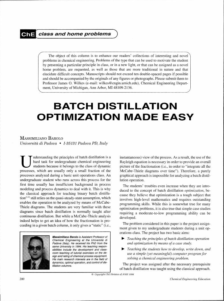
Solution of the problem requires the determination of the optimal reflux ratio for the operation of a given batch col­umn (the batch rectifier is shown in Figure 1). The objective function , P, (column productivity) is actually the same as the capacity factor CAP introduced by Luyben .131 The only dif­ference is that CAP is defined on a molar basis, while P is defined on a weight basis. The solution assumes that no costs are associated with by-product disposal. The feed mix­ture is also assumed to be at its boiling point.

The column productivity di­rectly accounts for two differ­ent effects of the reflux ratio on the column performance:

• A high reflux ratio in­creases the amount of dis­tillate product, D, eventu­ally collected, but it also increases the distillation time (i.e., the energy costs).

• A low reflux ratio results in a faster operation, but the amount of collected prod­uct decreases.

The column and reflux drum holdups are assumed to be neg­ligible in such a way that no differential equations need to

purge operations. An auto­matic system could be bought and installed if necessary, so that the changeover time could be reduced to about 0.5 h. The column is normally operated with a constant boil up rate of 50 kmol/h . The total fractionating capacity of the column is equivalent to

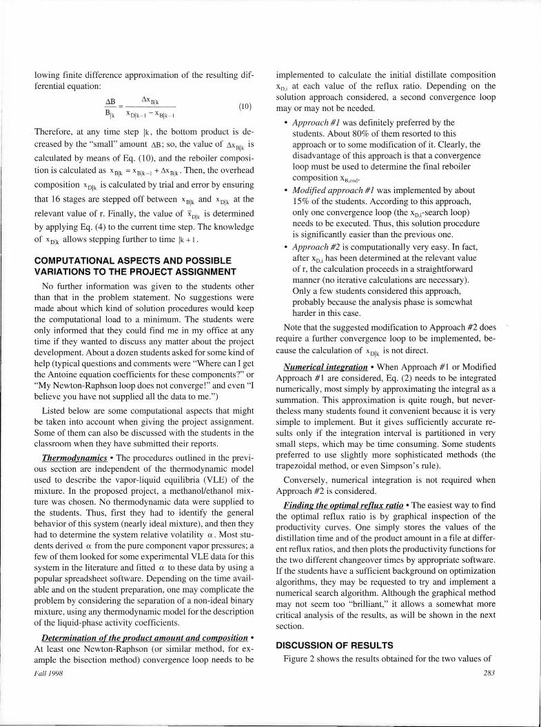
Figure 1. Sketch of the batch rectifier. be integrated for simulating the column (quasi-steady-state as-

16 theoretical stages (including the reboiler) . The column is a randomly packed one, so you will not endanger your calculations very much by assuming that the column holdup is negligible; the reflux drum holdup is also negligible.

The plant manager recommends keeping the column op­eration easy. "Operators are reluctant to change," he used to say. "They get used to operating the column at a constant reflux ratio; they need to operate the column that way! " He also wonders whether revamping the column (perhaps with a highly efficient structured packing) could bring any advan­tage. The sales office suggests that you evaluate the column productivity, P, through a simple formula:

P= Dw (kg/h) 1ctist + 1change

(I)

where Dw is the weight amount of methanol on specification, tdist is the distillation time, and tchange is the changeover time.

Now it ' s up to you! Money and Money, Inc. , expects that

Fall 1998

sumption). This allows the stu­dents to focus main] y on the characteristics of the distillation process rather than on the numerical aspects related to the integration of the system differential equations. Therefore, the computational time is minimized, allowing the project to be worked out easily on a PC. But in no way does this simplification relax the problem to a trivial one, as will be shown below.

The productivity function must be calculated at different values of the reflux ratio. For each value of the reflux ratio, the initial distillate composition, x0 ,; is first to be searched. The correct value of x0 _; is the one that enables 16 stages to be stepped off exactly between x0 _; and the feed composition, xF. Then, the problem can be tackled in different ways, some of which are illustrated below. A discussion on the ease of implementation of these approaches is given later.

Approach#]

As a consequence of the quasi-steady-state assumption, the total amount, B, of by-product accumulated in the reboiler

281

I_

at the end of the batch can be calculated through the Rayleigh equation 121

X 8 ,end

e B f dxs nF xo-xs

Xf

(2)

where x8 _end represents the reboiler composition at the end of the batch. The other symbols are listed in the Notation to this paper. This final composition is not known a priori, and must be searched numerically, a possible procedure for which is:

a) Choose one value r of the reflux ratio.

b) Determine the relevant value of Xo.i

c) Guess a value for Xs.end·

d) Run the simulation at a number of "slowly" decreas­ing values of the distillate (i.e., overhead vapor) composition x0 ; for each value of x0 , step off 16 stages in order to get the reboiler composition x8 .

e) Stop the simulation when x8 = Xs.end is found.

f) Evaluate B numerically through Eq. (2).

g) Estimate the accumulated distillate product composi­tion x0 by combining the total material balance

F=D+B (3)

with the more volatile component balance

(4)

h) If the value of x0 is not the desired one (i.e. , it is not

equal to the product specification xo,spec within a

specified tolerance), make a new guess for Xs,end and go back to d) until convergence is reached.

i) Calculate the distillation time, tdist :

(r+ l)D tdisl =--. -

V

j) Choose another value of the reflux ratio and restart from b).

Modified Approach #1

(5)

Basically, the calculations are the same as before, but the search of x8 _end is not performed by trial and error. Rather, after step b) has been executed, the calculation proceeds as follows:

c) Decrease the overhead composition by a "small" amount.

d) Starting from this new value of the overhead composi­tion , step off 16 stages and get the reboiler composi­tion .

e) Evaluate B numerically through Eq. (2).

f) Estimate the accumulated distillate product composi-

282

tion x0 by combining the total material balance and

the component balance.

g) If the value of x0 is not the desired one, go to c) in order to get a new overhead composition.

h) Calculate the distillation time through Eq. (5) .

i) Choose another value of the reflux ratio, and go to b) .

Approach#2

As a consequence of the quasi-steady-state assumption, the following balances hold at any time step lk:

Blk- 1 = Blk + t.Dlk

(x 8 B)lk-l = (x 8 B)lk + (xot.D)lk

(6)

(7)

where m1k is the amount of distillate product collected

between time steps lk - I and lk. By combining Eqs. (6) and (7),

X I -x I AD - Bk- I Bk B '-' lk - lk- 1

XDlk - XBlk

The calculation procedure is :

a) Choose one value for the reflux ratio.

b) Determine the relevant value of Xo.i and set

xDlk- 1 =xo,i•

c) Consider a "small" decrease t.x 0 of the overhead vapor composition, and set x01k = xDlk-l -t.xo.

(8)

d) Starting from x01k, step off 16 stages in order to get the bottom composition x81 k.

e) Using Eq. (8), calculate the corresponding increase t.o

1k of the amount of distillate product.

f) Calculate the corresponding increase t.(x 0 D)1

k of the more volatile component amount: t.(x 0 D)

1k = (x0 t.D)

1k.

g) Calculate the total amount o1k of distillate product

( o1k = Olk-I + t.o

1k) and the total amount of bottom

product ( B1k = B

1k-l - t.D

1k).

h) Calculate the total amount (x 0 D )1k of the more volatile

component in the distillate product:

(x 0 D)1k = (x 0 D)lk-l + t.(xoD)lk.

i) Evaluate the average distillate product composition :

_ (x 0 D)1k

XDl k =-- (9) Dlk

j) If the value of x0 is not the desired one, go to c) proceeding to time step lk + I .

k) Calculate the distillation time through Eq. (5).

1) Choose another value of the reflux ratio, and go to b).

A modification of this approach involves differentiating the Rayleigh equation (Eq. 2) and then considering the fol-

Chemical Engineering Educarion

lowing finite difference approximation of the resulting dif­ferential equation:

Af3 ~XBlk

B lk XDlk - 1 - XBlk-1 (LO)

Therefore, at any time step lk, the bottom product is de­

creased by the "small" amount Af3; so, the value of ~x BJk is

calculated by means of Eq. (10), and the reboiler composi­

tion is calculated as x 81k = x 8lk - J + ~xBJk . Then, the overhead

composition x01k is calculated by trial and error by ensuring

that 16 stages are stepped off between x81k and x01k at the

relevant value of r. Finally, the value of x01k is determined

by applying Eq. (4) to the current time step. The knowledge

of x01k allows stepping further to time lk + I.

COMPUTATIONAL ASPECTS AND POSSIBLE VARIATIONS TO THE PROJECT ASSIGNMENT

No further information was given to the students other than that in the problem statement. No suggestions were made about which kind of solution procedures would keep the computational load to a minimum. The students were only informed that they could find me in my office at any time if they wanted to discuss any matter about the project development. About a dozen students asked for some kind of help (typical questions and comments were "Where can I get the Antoine equation coefficients for these components?" or "My Newton-Raphson loop does not converge!" and even "I believe you have not supplied all the data to me.")

Listed below are some computational aspects that might be taken into account when giving the project assignment. Some of them can also be discussed with the students in the classroom when they have ubrnitted their reports.

Thermodynamics • The procedures outlined in the previ­ous section are independent of the thermodynamic model used to describe the vapor-liquid equilibria (VLE) of the mixture. In the proposed project, a methanol/ethanol mix­ture was chosen. No thermodynamic data were supplied to the students. Thus, first they had to identify the general behavior of this system (nearly ideal mixture), and then they had to determine the system relative volatility a. Most stu­dents derived a from the pure component vapor pressures; a few of them looked for some experimental VLE data for this system in the literature and fitted a to these data by using a popular spreadsheet software. Depending on the time avail­able and on the student preparation , one may complicate the problem by considering the separation of a non-ideal binary mixture, using any thermodynamic model for the description of the liquid-phase activity coefficients.

Determination of the product amount and composition • At least one Newton-Raphson (or similar method, for ex­ample the bisection method) convergence loop needs to be

Fall 1998

implemented to calculate the initial di stillate composition x0 _; at each value of the reflux ratio. Depending on the solution approach considered, a second convergence loop may or may not be needed.

• Approach# 1 was definitely preferred by the students. About 80% of them resorted to this approach or to some modification of it. Clearly, the disadvantage of this approach is that a convergence loop must be used to determine the final reboiler COmpOSition XB.end·

• Modified approach #1 was implemented by about 15% of the students. According to this approach, only one convergence loop (the x0 _;-search loop) needs to be executed. Thus, this solution procedure is significantly easier than the previous one.

• Approach #2 is computationally very easy. In fact, after x0 _; has been determined at the relevant value of r, the calculation proceeds in a straightforward manner (no iterative calculations are necessary). Only a few students considered this approach, probably because the_ analysis phase is somewhat harder in this case.

Note that the suggested modification to Approach #2 does require a further convergence loop to be implemented, be­cause the calculation of x01k is not direct.

Numerical integration • When Approach #1 or Modified Approach #1 are considered, Eq. (2) needs to be integrated numerically, most simply by approximating the integral as a summation. This approximation is quite rough, but never­theless many students found it convenient because it is very simple to implement. But it gives sufficiently accurate re­sults only if the integration interval is partitioned in very small steps, which may be time consuming. Some students preferred to use slightly more sophisticated methods (the trapezoidal method, or even Simpson's rule).

Conversely, numerical integration is not required when Approach #2 is considered.

Finding the optimal reflux ratio • The easiest way to find the optimal reflux ratio is by graphical inspection of the productivity curves. One simply stores the values of the distillation time and of the product amount in a file at differ­ent reflux ratios, and then plots the productivity functions for the two different changeover times by appropriate software. If the students have a sufficient background on optimization algorithms, they may be requested to try and implement a numerical search algorithm. Although the graphical method may not seem too "brilliant," it allows a somewhat more critical analysis of the results, as will be shown in the next section.

DISCUSSION OF RESULTS Figure 2 shows the results obtained for the two values of

283

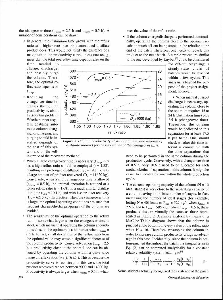
the changeover time (tchange = 2.5 h and tchange = 0.5 h). A number of considerations can be drawn.

ever the value of the reflux ratio.

• If the column charge/discharge is performed automati­cally, operating the column close to the optimum re­sults in much off-cut being stored in the reboiler at the end of the batch. Therefore, one needs to recycle this product to the next batch. A simple procedure similar to the one developed by LuybenC3J could be considered

284

• In general, the distillation time grows with the reflux ratio at a higher rate than the accumulated distillate product does. This would not justify the existence of a maximum in the productivity curve unless one recog­nizes that the total operation time depends also on the time needed to for off-cut recycling; a charge, di scharge, and possibly purge the column. There­fore, the optimal re­flux ratio depends on

600~~~.--,-------.-------.---.---.--r--r--r---r--,--,--,----,28 steady-state chain of batches would be reached within a few cycles. This analysis is beyond the pur­pose of the project assign-

tchange·

• Reducing the

570

,..._, 540 ..c c, 510 C, .?;- 480 ·s: :g 450 ::J -g 420 ,_ c. 390

/

24

20

✓------ 16

12

~--------~-, 8 - - - - - (dist (h)

4 .. ....... Ow/1000 (kg) 360'---''--'-~~~~~_._~..,___~.___,,~~--'

1.55 1.60 1.65 1.70 1.75 1.80 1.85 1.90 1.95

ment, however.

• When manual charge/ discharge is necessary, op­erating the column close to the optimum requires 15 to 24 h (distillation time) plus 2.5 h (changeover time). Therefore, the column would be dedicated to this

changeover time in­creases the column productivity by about 12% for this problem. Whether or not a sys­tem enabling auto­matic column charg­ing, discharging, and reflux ratio separation for at least 17 .5 purging should be in­stalled depends on the cost of this sys­tem and on the sell-

Figure 2. Column productivity, distillation time, and amount of distillate product for the two values of the changeover time.

h per batch. One should check whether this time in­terval is compatible with

ing price of the recovered methanol.

• When a large changeover time is necessary (tchange=2.5 h), a high reflux ratio should be employed (r "' 1.82), resulting in a prolonged distillation Ctctist "' 19.8 h), with a large amount of product recovered (Dw "' 11620 kg). Conversely, when a short changeover time is allowed (tchange = 0.5 h) , the optimal operation is attained at a lower reflux ratio (r "' 1.68), in a much shorter distilla­tion time (tdist "' 10.1 h) and with less product recovery (Dw"' 6215 kg) . In practice, when the changeover time is large, the optimal operating conditions are such that frequent charges/discharges/purges of the column are avoided.

• The sensitivity of the optimal operation to the reflux ratio is somewhat larger when the changeover time is short, which means that operating the column at condi­tions close to the optimum is a bit harder when tchange = 0.5 h. In fact, small deviations of the reflux ratio from the optimal value may cause a significant decrease of the column productivity. Conversely, when tchange = 2.5 h, a productivity close to the optimal one can be ob­tained by operating the column within a quite wide

range of reflux ratios ( r E [1.75; 1.9]) . This is because the

productivity curve is less steep; in this case, the total product recovered ranges between 9000 and 14000 kg. Productivity is always larger when tchange = 0.5 h, what-

the other separations that need to be performed in the same column during the production cycle. Conversely, with a changeover time of 0.5 h, only 10.6 h need to be allocated for each methanol/ethanol separation in this column. It might be easier to allocate this time within the whole production cycle.

• The current separating capacity of the column (N = 16 ideal stages) is very close to the separating capacity of a column having an infinite number of stages. In fact, increasing the number of ideal stages (for example, letting N = 40) leads to P max = 529 kg/h when tchange = 2.5 h, and to P max = 595 kg/h when tchange = 0.5 h; these productivities are virtually the same as those repre­sented in Figure 2. A simple analysis by means of a McCabe-Thiele diagram shows that the column is pinched at the bottom for every value of the reflux ratio when N = 16. Therefore, revamping the column in order to increase column productivity brings no advan­tage in this case. Incidentally, since the column is bot­tom-pinched throughout the batch, the integral term in Eq. (2) can be computed analytically for a constant relative volatility system, leading tol41

fo - = -- Rn --+ -- fo _::_-,---'"7 B I [ 1-xp I xs(l-xp)] F r+l l- x8 a-1 xF(l-x 8 )

(11)

Some students actually recognized the existence of the pinch

Chemical Engineering Education

point, so they avoided performing the numerical evalu­ation of the integral term.

FINAL REMARKS

The feedback from the students on this assignment was good. They liked working on a project that resembles a real­life problem. The time needed for writing the program and studying the results was not too long. Many of the findings outlined in the previous section were spotted by students. In any case, the alternative solution procedures and the results were finally di scussed in the classroom.

The project proved to be very instructive, but it appears to be oversimplified for use at a graduate level. In this case, one may have a look at Diwekar' s textbookcsi in order to get useful instructive material on advanced batch distillation design, simulation, and optimization.

ACKNOWLEDGMENT

I would like to thank Prof. Gian Berto Guarise for helpful discussions. Support by MURST (jondi 60%) is gratefully acknowledged.

NOTATION

B bottom product (kmol) CAP column capacity factor (kmol/h)

D distillate product (kmol) D w distillate product (kg)

F feed charge (kmol) P column productivity (kg/h)

Pm"" maximum column productivity (kg/h) r reflux ratio

tchangc changeover time (h) tdisi distillation time (h) v vapor boilup rate (kmol/h) x

8 reboiler composition (mole fraction)

x8 _end final reboiler composition (mole fraction) x

0 overhead vapor composition (mole fraction)

x0 average distillate product composition (mole fraction)

xo.spec specification on the average distillate product composition

(mole fraction) xF feed composition (mole fraction)

a relative volatility t:,. increase

lk k-th time step

REFERENCES 1. Coulson, J.M. , and J.F. Richardson, Chemical Engineering,

Vol. 2, Pergamon Press, Oxford, United Kingdom (1991) 2. McCabe, W.L., J .C. Smith, and P . Harriott, Unit Operations

of Chemical Engineering, McGraw-Hill Book Co., New York, NY(1993)

3. Luyben, W.L., ''Multicomponent Batch Distillation. 1. Ter­nary Systems with Slop Recycle," Ind. Eng. Chem. Res., 27, 642 (1988)

4. Guarise, G.B., Distillation, Absorption and Liquid-Liquid Extraction for University Students (in Italian), CLEUP,

Fall 1998

Padova, Italy (1996) 5. Diwekar, U.M. , Batch Distillation: Simulation, Design, and

Control, Taylor & Francis, London, United Kingdom (1995) 0

Book Review: Phase Equilibria Continued from page 277

pressure VLE and, in Chapter 9, they describe equilibrium cells for multiphase, high-pressure systems. The focus of both of these chapters is on the authors' own work, and it is written with a level of detail that one would typically find in a dissertation. Particular attention is given to experimental difficulties (usually related to sampling) and techniques to address them. For this reason, these chapters will be useful to anyone who plans to build a high-pressure apparatus­even one based on a different design.

Part 3 of the book covers low-pressure phase equilibria computations and includes chapters that cover correlative methods for activity coefficients (Chapter 10), flash calcula­tions (Chapter 11), predictive methods for activity coeffi­cients (Chapter 12), and liquid-liquid calculations (Chapter 13). Part 4 covers calculations at high pressure, including background information (Chapter 14 ), equation-of-state meth­ods (Chapter 15), gamma-phi methods (Chapter 16), and mixing rules (Chapter 17). The book concludes with Chapter 18, which discusses thermodynamic consistency testing.

Parts 3 and 4 of the book do not have the breadth of Phase Equilibria in Chemical Engineering by Walas or of Proper­ties of Gases and Liquids by Reid, Prausnitz, and Poling. But they are written at the depth of the former, and the breadth is consistent with the experimental techniques that are described. The discussions of mixing rules and consistency tests, and the relation between VLE and heat of mixing, are more detailed than are generally found in other books. Topics that aren't covered in extreme detail, such as methods for inte­grating the coexistence equation, are accompanied by enough references that the reader may find the details elsewhere.

This book will be of limited use as a textbook because it contains no exercises. But I believe that its coverage of experimental methods will be highly useful to anyone who measures phase equilibria. I know that it would have saved me months of work had it been available a number of years ago. The sections on computations will probably not (due to limited breadth) be a primary source of information on this topic, but they will be a useful supplement since they are current and cover several topics that are given only passing mention in other references.

I have additional criticism about the organization of the book, and I noticed a number of typographical errors and a missing figure. But the first criticism is probably a personal prejudice and the second should be fixed in the next printing. None of these minor complaints will prevent my copy of the book from receiving a lot of use. 0

285