1 DYNAMIC MONEY DEMAND FUNCTION FOR ETHIOPIA 1 Berhanu Denu 2 Abstract This study has estimated stable long run and dynamic money demand equations for Ethiopia. However, the study shows some portfolio demand adjustment by agents after liberalization of asset prices after 1992. The study, by estimating money demand using disaggregated price level, shows that livestock, money and housing items are complements, and money and all other goods are substitutes in the portfolio demand of Ethiopian agents. The study suggests that the government should follow a sound trade policy, strengthen the development of exchange oriented rural economy, use depreciation of currency than domestic credit control, facilitate conditions for the development of capital market and strengthen policy of indirect monetary control, and privatization to achieve sustainable growth and development. The study also suggests that the government should look for an alternative higher rate of inflation rather than targeting it to a low rate of single digit, which might hinder accelerated growth. 1. Introduction The demand for money is a heavily researched area of economics. This is due to the important role of private economic agents’ behavior in determining the outcome of economic policy reform that target monetary aggregates. However, much of the empirical research has focused on developed economies. This study focuses on a developing country. Empirical research has also concentrated on the identification of the appropriate key economic variables that determine the amount of real money 1 The final version of this article was submitted in September 2006. 2 [email protected] ; Tel: 091 40 9027 Acknowledgements: I am obliged to extend my heartfelt appreciation to the AERC (African Research Consortium) for finding the study. I am also indebted to the generous suggestions, comments and technical assistance by the resource persons, and external evaluators.

Welcome message from author
This document is posted to help you gain knowledge. Please leave a comment to let me know what you think about it! Share it to your friends and learn new things together.
Transcript

1
DYNAMIC MONEY DEMAND FUNCTION FOR ETHIOPIA1
Berhanu Denu2
Abstract
This study has estimated stable long run and dynamic money demand equations for Ethiopia. However, the study shows some portfolio demand adjustment by agents after liberalization of asset prices after 1992. The study, by estimating money demand using disaggregated price level, shows that livestock, money and housing items are complements, and money and all other goods are substitutes in the portfolio demand of Ethiopian agents. The study suggests that the government should follow a sound trade policy, strengthen the development of exchange oriented rural economy, use depreciation of currency than domestic credit control, facilitate conditions for the development of capital market and strengthen policy of indirect monetary control, and privatization to achieve sustainable growth and development. The study also suggests that the government should look for an alternative higher rate of inflation rather than targeting it to a low rate of single digit, which might hinder accelerated growth.
1. Introduction The demand for money is a heavily researched area of economics. This is due to the important role of private economic agents’ behavior in determining the outcome of economic policy reform that target monetary aggregates. However, much of the empirical research has focused on developed economies. This study focuses on a developing country. Empirical research has also concentrated on the identification of the appropriate key economic variables that determine the amount of real money
1 The final version of this article was submitted in September 2006. 2 [email protected]; Tel: 091 40 9027 Acknowledgements: I am obliged to extend my heartfelt appreciation to the AERC (African Research Consortium) for finding the study. I am also indebted to the generous suggestions, comments and technical assistance by the resource persons, and external evaluators.
Berhanu Denu: Dynamic money demand function for Ethiopia
2
balances that economic agents want to hold. Thus, the most common money demand specification includes real income as a measure of scale variable, one or more measures of the opportunity cost of holding money, lagged value of the dependent variable and dummy variables to account for seasonal variations and regime shifts. Most of the empirical studies have employed aggregate real income, the rate of general inflation and other variables as explanatory variables. However, some researchers have used disaggregated income as non-monetized and monetized components in studies on developing countries, see Arize, Darrat and Meyer(1990), Driscoll and Lahiri (1983), Laumas (1978). This study also employs disaggregated income as rural and urban income and both components of income are included in the model. It is to be noted that the Ethiopian economy is agriculture dominated and the change in the share of rural and urban income can have a significant influence on the demand for money. In addition to the agrarian nature of the economy, livestock ownership is of greater importance in the asset portfolio of the representative household. Thus the study employs disaggregated rate of price level as price of livestock, prices of housing and housing items and prices of all other goods. The finding of the study is expected to improve information on the estimation approach in money demand studies in developing economies. During the last decade of the 20th century, most of African countries south of the Sahara started to implement economic liberalization measures and structural adjustment programs (SAP). This changed situation has made empirical investigation of money demand to remain of interest to researchers. Ethiopia is one of the sub-Saharan African countries which have embarked on structural adjustment program. The reform measures implemented so far have changed the prices of assets and this change might have affected the demand for cash balances. Furthermore, Ethiopia is a small developing economy with heavy dependence on external assistance. This situation makes the behavior of domestic agents to be strongly influenced by external economic and monetary development. This makes it appropriate to include a variable that measures changes in foreign interest rat + exchange rate. The purpose of the study is to identify the demand for narrow and broad money with particular attention to the ongoing policy change, the agrarian nature of the economy, the important role of livestock, the heavy external dependence and the long instability and civil war in the country.
Ethiopian Journal of Economics, Volume XII, No 2, October 2003
3
The objective of the study The main objective is to estimate dynamic money demand equations for narrowly defined money (m1) and broadly defined money (m2) in order to provide information for monetary policy makers. The specific objectives include:
a) To estimate the elasticity of money demand with regard to explanatory variables in the money demand function for Ethiopia,
b) To study the effect of dis-aggregation of income and price level on the aggregate demand function.
c) To provide policy recommendation. The study is organized as follows: Section II presents a review of selected theoretical and empirical works on the demand for money in Africa. Section III deals with issues of methodology. Section IV discusses empirical application, data sources, and data description. Section V presents empirical findings and analysis of the findings. Finally Section VI concludes the paper with a brief implication of policy and conclusion.
2. Empirical studies on demand for money in Africa One of the major studies on money demand in Africa is the work of Domowitz and Elbadawi (1987). The authors estimated the demand for narrow money (currency + demand deposit) for the Sudan. The data are annual and the sample period is 1956:1982. The explanatory variables are real GDP, the rate of inflation and the official exchange rate of the Sudanese pound against the dollar. Domowitz and Elbadawi specified a stable demand function for money by employing the error correction modeling (ECM) for data on a small open economy. Due to the undeveloped financial sector of the Sudan, the authors attached a greater importance to the rate of inflation in their analysis. Another important study on money demand on Africa is that of Adam (1992). Adam uses quarterly data to estimate the demand for M0 (currency in circulation), M1 (currency demand deposit), M2 (M1 + Time and Savings deposit), M3 (M2 + deposit liabilities of non bank financial institutions). In the case of M3, both its simple aggregate and the Divisia version are used. The explanatory variables in Adam include GNP adjusted for changes in the terms of trade (the quarterly figure is obtained by interpolation), the consumer price index (CPI), the government regulated Treasury bill rate, and the expected rate of domestic
Berhanu Denu: Dynamic money demand function for Ethiopia
4
currency depreciation, which is approximated by the rate of change of the domestic parallel market exchange rate. Adam's findings show that there is a long run stable relationship between the demand for the different aggregates of money on the one hand and the explanatory variables on the other. Simons (1992) undertook an important work on African economies. Simons estimated the demand for narrow money (M1) for five African countries. The countries included in the study were Congo, Cote d'Ivoire, Mauritius, Morocco and Tunisia. The findings show that in three of the countries the rate of interest plays an important role. On the other hand, the rate of inflation and exchange rate are significant in explaining the demand for money in countries where information on the rate of interest is lacking, and the rate of inflation is higher. Simons argues that it is irrelevant to exclude the rate of interest from money demand in the developing countries during the present era of financial liberalization and structural adjustment. A further important study on Africa is that of Fielding (1993). Fielding used quarterly data to estimate the demand for money function in four African countries- Kenya, Nigeria, Cameroon and Cote d'Ivoire. Fielding estimated the demand for M2 (money + quasi money) for the sample period 1978-1989 (the sample periods are slightly different for the different countries). The explanatory variables considered include GDP (the quarterly figure is obtained by interpolation), the central bank discount rate or Treasury bill rate, the parallel market exchange rate and the consumer price index. The findings show significant variations among the countries studied. Consequently, Fielding concludes that it is impossible to formulate a single monetary policy applicable to the different countries, implying the potential difficulty of a possible monetary union. Fielding's study indicates the necessity of further investigation of money demand function in the developing countries. An important study was also conducted for seven African countries (Egypt, The Gambia, Mauritania, Morocco, Niger, Nigeria and Somalia (see Arize, Darrat and Meyer, 1990). The authors found that domestic money holdings are significantly related to monetized income and external influences. Hoffman, D and Tahiri, C. (1994) are among those who studied money demand in Africa. They made use of a foreign (Swiss) Treasury bill rate to estimate the demand for money for Morocco. The authors reported their success in specifying a stable long run demand function for M1 & M2, implying that it is advisable to use a foreign rate of interest rather than completely ignoring the rate of interest in the developing countries.
Ethiopian Journal of Economics, Volume XII, No 2, October 2003
5
Sriram (IMF, 2001) presented a survey of empirical money demand studies with error correction model approach, which were conducted in the 1990s across different countries. The paper presents a summary of the cointegration technique used, the variables, the data period and frequency, unit root test, long run income elasticity and elasticity or semi-elasticity for opportunity cost variables and other variables. The paper is of greater importance as a reference for further research. Studies on money demand in Ethiopia are rare, and even the few work studies undertaken are in the form of unpublished MSC theses. Of these the most representative ones are discussed below. One of the few studies is Samuel Mulugeta’s (2005) ‘The Demand for Money and Monetary policy in Ethiopia.’ The sample period for the study is 1970q1, to 2003/04q4. The variables included in the study are real narrow money balance, real GDP, the saving deposit rate, the inflation rate, the parallel market depreciation rate of the birr. Both the long run and short run functions were estimated. The Johansen procedure was used in the process. The study found a 1.12 long run income coefficient and an inflation rate coefficient of -12.5. Income and past money holdings were found to affect the short run function. While this can be taken as a good work, there are some points of gaps. The first point relates to the author’s rationale for dropping out the depreciation rate. The author a priori determined that the depreciation rate should take a negative sign. This is incorrect, since the variable can take either positive or negative values. Another point of contention can be the way the author used the dummy variables. Rather than mentioning the names of the dummies, the values they were given were not explicitly presented. This is necessary since the Johnson test is affected by the type of the values the dummies take. For instance, the 0/1 seasonal dummy is not appropriate for the Johansen procedure. There should be centered seasonal dummies the value of which should add up to zero. The use of step dummies may also generate trends on the levels of variables, (see Doornick, Hendry and Nielson, 1998, Arize, Malidretos and Shwiff, 1999) Still another point of weakness relates to the way stationarity is established. In Johansen procedure individual unit root test using DF/ADF prior to the estimation of the co integrating vectors are identified. However, the multivariate test is more appropriate in Johansen approach (see Johansen 1995). Also the result of income homogeneity imposition was not presented. This is necessary since the reported income coefficient of the long run equation is in excess of unity. However the paper contains a number of interesting findings and good information on the financial sector of Ethiopia.
Berhanu Denu: Dynamic money demand function for Ethiopia
6
In conclusion, the following points can be made about empirical studies in money demand on developing economies.
a) There is still room for empirical studies of the subject in order to cover the many developing countries in the face of the changing economic and policy environment.
b) Past studies show the fact that modern econometric technique can be applied to data on developing countries.
c) The choice of explanatory variables should be left to empirical test rather than apriori netting out of some variables such as the rate of interest.
d) There are variations across countries and this implies variations in monetary policies of the different countries.
3. Model specification and theoretical considerations The money demand function must be defined before undertaking any empirical analysis. In economic theories of money demand, there are at least two reasons why money may be demanded. The first is as an inventory to smooth differences between income and expenditure streams, and the second is as one among several assets in a portfolio. Money in the representative agent model The conceptual framework for money demand functions can be sought in the representative agent models. These models deal with the portfolio holding of agents. Money is entered in the utility function, and the demand for money is derived from the utility maximizing behavior of the representative agent. Such an approach was used by Tobin (1965), and Sidrauski (1967). Both of these works investigated money demand in relation to economic growth. Tobin concluded that agents allocate a fixed amount of saving, whereas Sidrauski argued that money demand was to be derived from utility maximizing behavior of agents. The asset portfolio approach has been employed in the study of money demand in Sub-Sahara African countries. Among those who applied the approach are Adam (1999) and Randa (1999) in their studies on Zambia and Tanzania respectively. The same approach is used in this study to identify money demand function for Ethiopia.
Ethiopian Journal of Economics, Volume XII, No 2, October 2003
7
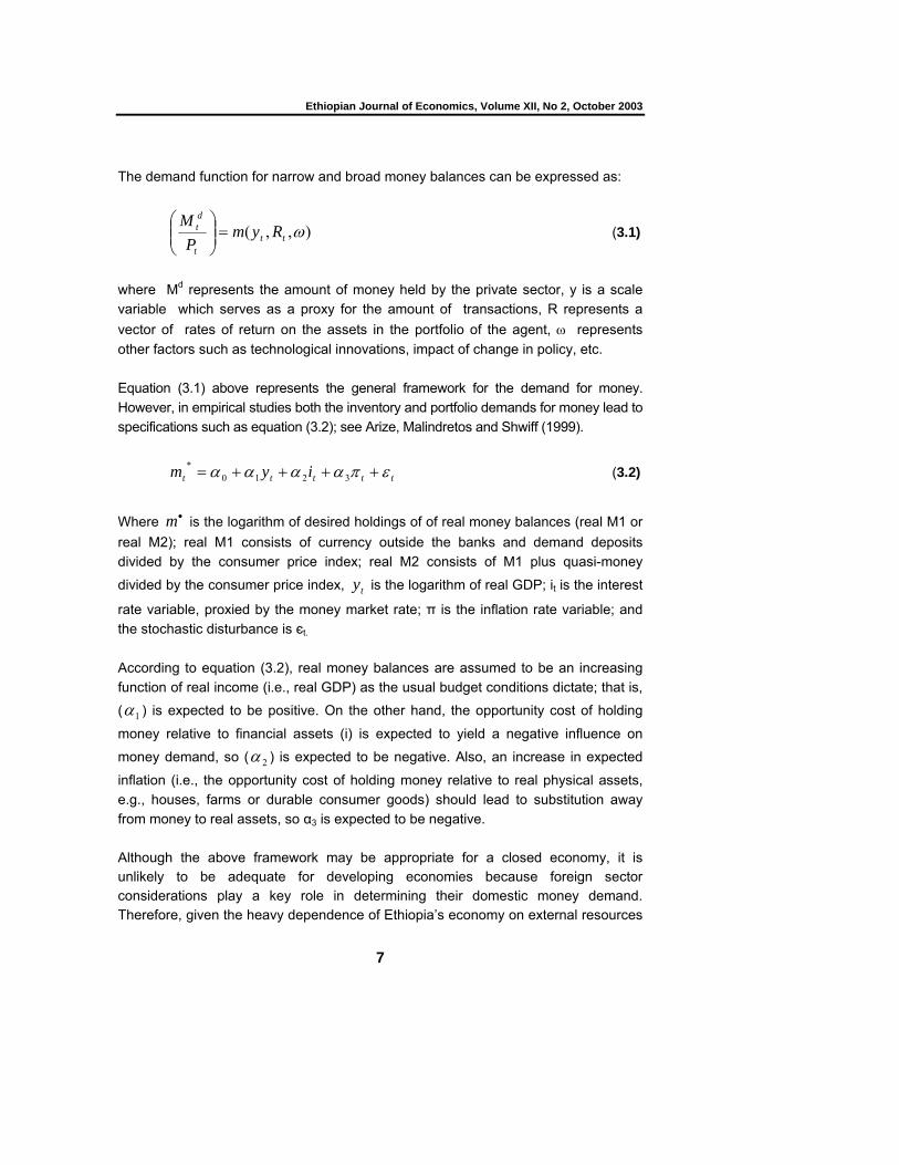
The demand function for narrow and broad money balances can be expressed as:
),,( ωttt
dt Rym
PM
=⎟⎟⎠
⎞⎜⎜⎝
⎛ (3.1)
where Md represents the amount of money held by the private sector, y is a scale variable which serves as a proxy for the amount of transactions, R represents a vector of rates of return on the assets in the portfolio of the agent, ω represents other factors such as technological innovations, impact of change in policy, etc. Equation (3.1) above represents the general framework for the demand for money. However, in empirical studies both the inventory and portfolio demands for money lead to specifications such as equation (3.2); see Arize, Malindretos and Shwiff (1999).
ttttt iym επαααα ++++= 3210* (3.2)
Where •m is the logarithm of desired holdings of of real money balances (real M1 or real M2); real M1 consists of currency outside the banks and demand deposits divided by the consumer price index; real M2 consists of M1 plus quasi-money
divided by the consumer price index, ty is the logarithm of real GDP; it is the interest
rate variable, proxied by the money market rate; π is the inflation rate variable; and the stochastic disturbance is єt. According to equation (3.2), real money balances are assumed to be an increasing function of real income (i.e., real GDP) as the usual budget conditions dictate; that is,
( 1α ) is expected to be positive. On the other hand, the opportunity cost of holding
money relative to financial assets (i) is expected to yield a negative influence on
money demand, so ( 2α ) is expected to be negative. Also, an increase in expected
inflation (i.e., the opportunity cost of holding money relative to real physical assets, e.g., houses, farms or durable consumer goods) should lead to substitution away from money to real assets, so α3 is expected to be negative. Although the above framework may be appropriate for a closed economy, it is unlikely to be adequate for developing economies because foreign sector considerations play a key role in determining their domestic money demand. Therefore, given the heavy dependence of Ethiopia’s economy on external resources
Berhanu Denu: Dynamic money demand function for Ethiopia
8
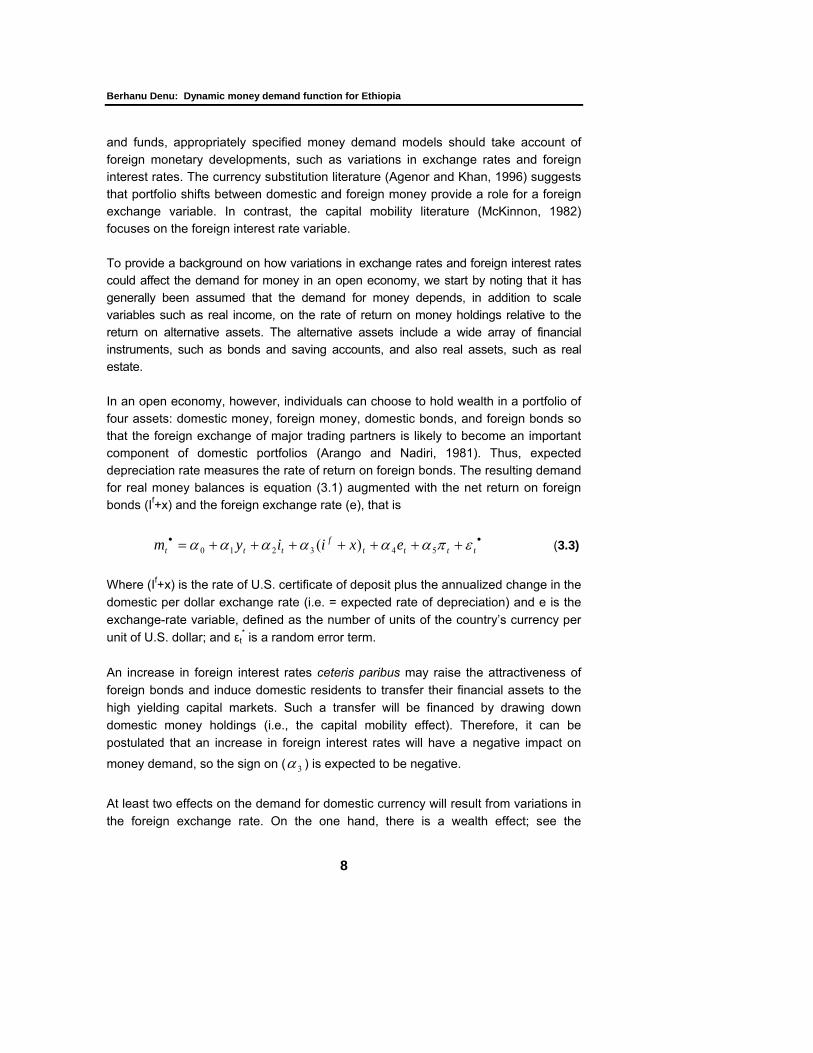
and funds, appropriately specified money demand models should take account of foreign monetary developments, such as variations in exchange rates and foreign interest rates. The currency substitution literature (Agenor and Khan, 1996) suggests that portfolio shifts between domestic and foreign money provide a role for a foreign exchange variable. In contrast, the capital mobility literature (McKinnon, 1982) focuses on the foreign interest rate variable. To provide a background on how variations in exchange rates and foreign interest rates could affect the demand for money in an open economy, we start by noting that it has generally been assumed that the demand for money depends, in addition to scale variables such as real income, on the rate of return on money holdings relative to the return on alternative assets. The alternative assets include a wide array of financial instruments, such as bonds and saving accounts, and also real assets, such as real estate. In an open economy, however, individuals can choose to hold wealth in a portfolio of four assets: domestic money, foreign money, domestic bonds, and foreign bonds so that the foreign exchange of major trading partners is likely to become an important component of domestic portfolios (Arango and Nadiri, 1981). Thus, expected depreciation rate measures the rate of return on foreign bonds. The resulting demand for real money balances is equation (3.1) augmented with the net return on foreign bonds (If+x) and the foreign exchange rate (e), that is
•• +++++++= ttttf
ttt exiiym επαααααα 543210 )( (3.3)
Where (If+x) is the rate of U.S. certificate of deposit plus the annualized change in the domestic per dollar exchange rate (i.e. = expected rate of depreciation) and e is the exchange-rate variable, defined as the number of units of the country’s currency per unit of U.S. dollar; and εt
* is a random error term. An increase in foreign interest rates ceteris paribus may raise the attractiveness of foreign bonds and induce domestic residents to transfer their financial assets to the high yielding capital markets. Such a transfer will be financed by drawing down domestic money holdings (i.e., the capital mobility effect). Therefore, it can be postulated that an increase in foreign interest rates will have a negative impact on
money demand, so the sign on ( 3α ) is expected to be negative.
At least two effects on the demand for domestic currency will result from variations in the foreign exchange rate. On the one hand, there is a wealth effect; see the

Ethiopian Journal of Economics, Volume XII, No 2, October 2003
9
discussions, for instance, by Arango and Nadiri (1981). Assume that wealth holders will evaluate their asset portfolios in terms of their domestic currency. Therefore, when domestic currency depreciates, there will be an increase in the value of foreign assets held by domestic residents (i.e., wealth-enhancing effect). This in turn leads to a rebalancing effect because, in order to maintain a fixed share of their wealth invested in domestic assets, they will repatriate part of their foreign assets to domestic assets, including domestic currency (i.e. rebalancing). As Arango and Nadiri (1981, P.79) have argued, it is because of the “rebalancing effect” brought about by changes in the exchange rate, that an exchange rate depreciation has a positive effect on the demand for money. Hence, exchange rate depreciation would increase the demand for domestic currency. On the other hand, variations in the exchange rate can generate a currency substitution effect in which a key role is played by investors’ expectations. According to the currency substitution literature, as a weak domestic currency develops expectations for further weakening, asset holders will respond by shifting some of their portfolios away from domestic currency into foreign assets. So, if depreciation of Ethiopia’s Birr reflected by an increase in exchange rate induces a decline in money holding by domestic residents, the estimate of 4α should be negative. To summarize,
the expected signs for equation (3.3) are 1α >0, 2α , 3α , 4α , 5α < 0, 4α > 0. Based
on the above discussions, an increase in the exchange (i.e., depreciation) could have a positive or negative effect on the demand for money; therefore, which effect dominates is an empirical issue, see Arango and Nadiri (1981), Arize(1989), Bahamani and Pourheydarian (1990), Arize, Darrat and Meyer(1990), Arize and Shwiff(1998), Arize, Malindretos and Shwiff(1999). Equations (3.2) and (3.3) have assumed that the money market is in equilibrium, and they may be viewed as co integration models. The basic idea of co integration is that two or more non stationary time series may be regarded as defining a long-run equilibrium relationship if a linear combination of the variables in the model is stationary (converges to an equilibrium over time). Thus, if the money demand function in equation (3.2) or (3.3) describes a stationary long-run relationship among the variables in these equations, this can be interpreted to mean that the stochastic trend in real money balances is related to the stochastic trends in the real income, the interest rate and external monetary factors. In other words, even though deviations from the equilibrium should occur, they are meant reverting.

Berhanu Denu: Dynamic money demand function for Ethiopia
10
4. Empirical application 4.1 Data description The data set used in this study consist of seasonally unadjusted quarterly M1 (narrow money), M2 (broad money), real Gross Domestic Product (Y), the consumer price index (PI), the parallel market exchange rate (bdep), the inflation rate (dinfr), rural income(yr), urban income (uy), deposit rate (i), and a combination of foreign interest rate and the rate of exchange, the price of live animals (Pa), price of household items (Ph), prices of all other goods (Px), a measure of domestic credit as a ratio of GDP (ci), centered seasonal dummies, blimps(impulse) and shift dummies. Only real variables are used in the analysis in order to maintain long run price homogeneity of the demand for money. The sample period is the period (1974Q1: 2004Q4. The data are obtained from the National Bank of Ethiopia (NBE) and the Picks World Currency yearbook. The quarterly figures for GDP are constructed from annual figures using Goldstein’s interpolation technique (see Goldstein, 1976). Quarterly monetary aggregates have been constructed from monthly figures obtained from the National Bank. Quarterly prices have been formed from annual figures using the equation
Pn = n
n PPP
1
1
21 ⎟⎟
⎠
⎞⎜⎜⎝
⎛− ,that is, the nth root of the ratio of change during the year
multiplied by the preceding value where “n” stands for quarter period(n = 1…4), P1 and P2 represent the price level at the beginning and at the end of the year respectively. Quarterly prices of live animals have been calculated from export value index and quantity index for live animals since a reliable time series data are not available.
Value index (relative) = 00QP
QP tt X100, Quantity index (relative) = 0Q
Qt X100
Price index = 0000 P
PQQ
QPQP
dexQuantityinValueindex tttt =÷=÷ X100
The price index of livestock obtained in this manner should be treated with caution. The scale variables after 1992 include the figures for Eritrea which have been
Ethiopian Journal of Economics, Volume XII, No 2, October 2003
11
obtained from the Economic Intelligence in part and by estimating the missing years. The end of the “Birr Zone” has been taken care of by adding a dummy variable for the year 1997. The nominal figures for GDP, GNP and GDE are deflated by the consumer price index CPI, to obtain real figures. The CPI is preferable in that it includes imports which consumers buy while it excludes exports which are not consumed domestically. The weakness of the CPI is that it excludes expenditures on investment but these are a smaller proportion of the total expenditures. Despite the fact that the rate of interest in Ethiopia has been state regulated for a long time, it is included as an explanatory variable due to the importance of the variable in money demand functions and for monetary policy exercise. The rate of domestic inflation is included in the equation as a domestic opportunity cost of holding money. The parallel market exchange rate is also included in this study in order to capture the external opportunity cost of holding domestic currency. The exchange rate is expressed in terms of units of domestic currency per unit of foreign currency. Hence, a rise in the rate of exchange means depreciation of the domestic currency. Ethiopia has been under unstable political and economic condition. These changes are assumed to be exogenous and are accounted for by dummy variables. Thus dummy variables are included to account for the changes in political power in 1974, 1991, the Ethio-Eritrean conflict in 1997 and several additional liberalization measures in 1998. 1974 was the year when the military deposed Emperor Haile Sellasie and seized power. The dummy variable for this year is denoted as D974. The year 1991 was the year in which the military government entered its final phase of countrywide crisis and power passed into the hands of the EPRDF. The dummy variable for 1991 is denoted by D991. In 1997 a crisis started between Eritrea and Ethiopia. A dummy variable denoted D997 is used to account for this change. All of these dummy variables are impulse or blimp dummies taking the value of 1 for the year of the changes and 0 otherwise. Thus D974 is given 1 for 1974Q1 and 0 for other periods. D991 takes the value of 1 for 1991Q2 and 0 for other years. D997 is given 1 for 1997Q2 and 0 for the remaining years. The quarters represent the periods of the changes. Three other dummies, D992, D994 and D998, are also included to account for the 1992 devaluation of the Birr, the 1994 monetary and banking reform and the 1998 further liberalization of the foreign exchange operations and the lending rate. In 1998, measures like the abolition of the ceiling on the lending interest rate, redenomination of T-bills from birr 50,000 to birr 500, the move from retail forex auction to wholesale auction, elimination of the foreign exchange surrender requirement, and the liberalization
Berhanu Denu: Dynamic money demand function for Ethiopia
12
of the restrictions relating to foreign exchange transactions for education business travel and health. These dummies are transitory dummies and take the value of (1) for the years of the changes and the value of (-1) in the year following the change and zero for the remaining years. Hence D992 takes 1 for 1992 and (-1) for 1993 and (0) for the other years. D994 takes (1) for 1994, (-1) for 1995 and (0) for the rest of the years. In addition to these shift dummies, seasonal dummies in the form of sc1, sc2, sc3, and sc4 are used to account for seasonal variations in the variables. The seasonal dummies are centered dummies taking the value of 0.25 for the first three quarters and -0.75 for the fourth quarters. 4.2 The time series characteristics of the data The first step in testing for co-integration in a set of variables is to test for stochastic trends in the autoregressive representation of each individual time series using the augmented Dickey and Fuller and Johansen tests. It is found in Table 3 below that the null hypothesis of non-stationarity is accepted when the variables are in levels. In addition, for the Johansen test, the null hypothesis of stationarity is rejected in each case. Hence, all the variables are assumed as non-stationary in levels for the purpose of estimating the demand for money. 4.3 Estimation method The long run money demand is estimated using the following equation:
tttttd Rym εφγβα ++++= 4.3.1
Where y = log of real income Rt = a vector of the opportunity cost of holding money and includes the expected rate of inflation, the rate of interest on interest bearing deposits and foreign (US) treasury bill rate as well as the parallel market rate of depreciation.
φ = a vector of deterministic variables which include seasonal and other dummies as
well as variables like time trend that captures regime shifts in money demand, α is a
constant, β is constant income elasticity, and γ is constant elasticity or semi elasticity of the opportunity cost variables (Rt). And with the assumption of long run price homogeneity, real money balances increase in real income and decrease in inflation.
The vector can be defined as ⎟⎟⎠
⎞⎜⎜⎝
⎛⎟⎠⎞
⎜⎝⎛+
⎟⎠⎞
⎜⎝⎛+
=exr
exrifexiymX t 1,
inf1inf,,,, 4.3.2

Ethiopian Journal of Economics, Volume XII, No 2, October 2003
13
The dynamic money demand function is represented by the multivariate co-integrating-vectors approach within the error correction framework. The error correction vector auto regression model is in the following form:
∆Xt = Φ1∆Xt- 1+ αβ ′Xt- 1+δZt+Ω t+ε t 4.3.3 Where: ∆Xt represents the first difference of I(1) variables αβ′Xt-1 denotes the reduced rank matrix of long run co-integrating vectors of I(1) variables, Zt represents other stationary variables that are restricted to lie outside the co-integrating space, α represents the speed of adjustment towards long-run equilibrium by the variables whenever there is deviation from equilibrium, Ωt denotes a vector consisting of an intercept, three centered seasonal dummies, and other dummies accounting for regime shift.
5. Empirical findings 5.1 The demand for narrow and broad money The long run demand for narrow and broad money has been specified using Johansen’s approach. Both the likelihood ratio, based on Eigen values, and trace statistic show the existence of three co-integrating vectors combining log of real narrow and broad money (m1,m2), real gross domestic product(y), the rate of inflation, parallel market exchange rate, log of deposit rate and log of (US certificate of deposit + domestic parallel market exchange rate), lifex. Of the three co-integrating vectors, the ones with the theoretically acceptable sign of coefficients are presented below for analysis.
m1 y dinfr bdep i ifex β -1.00 0.7999 – 1.5954 7.06 - -.2209 α 0.08 -0.03 0.03 -0.011 - 0.01 ß -1.00 .816 -2.821 1.362 27.6 -1.813 α (0.114) (-0.044) (0.03) (-0.012) (-0.009) (0.009)
The β vector represents the long-run equilibrium linear combination of I (1) variables whereas α represents the speed of adjustment towards long-run equilibrium when economic agents are out of equilibrium. Thus about 8% of the disequilibria in the demand for narrow money and 11% of the demand for broad money are corrected per each quarter, and this is relatively a lower speed of adjustment. However, the coefficients are signed as expected. The coefficient for income is expected to lie
Berhanu Denu: Dynamic money demand function for Ethiopia
14
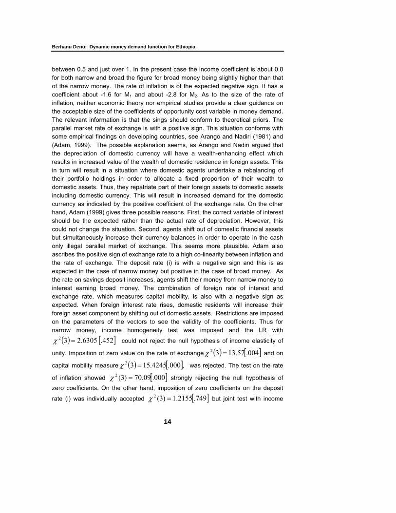
between 0.5 and just over 1. In the present case the income coefficient is about 0.8 for both narrow and broad the figure for broad money being slightly higher than that of the narrow money. The rate of inflation is of the expected negative sign. It has a coefficient about -1.6 for M1 and about -2.8 for M2. As to the size of the rate of inflation, neither economic theory nor empirical studies provide a clear guidance on the acceptable size of the coefficients of opportunity cost variable in money demand. The relevant information is that the sings should conform to theoretical priors. The parallel market rate of exchange is with a positive sign. This situation conforms with some empirical findings on developing countries, see Arango and Nadiri (1981) and (Adam, 1999). The possible explanation seems, as Arango and Nadiri argued that the depreciation of domestic currency will have a wealth-enhancing effect which results in increased value of the wealth of domestic residence in foreign assets. This in turn will result in a situation where domestic agents undertake a rebalancing of their portfolio holdings in order to allocate a fixed proportion of their wealth to domestic assets. Thus, they repatriate part of their foreign assets to domestic assets including domestic currency. This will result in increased demand for the domestic currency as indicated by the positive coefficient of the exchange rate. On the other hand, Adam (1999) gives three possible reasons. First, the correct variable of interest should be the expected rather than the actual rate of depreciation. However, this could not change the situation. Second, agents shift out of domestic financial assets but simultaneously increase their currency balances in order to operate in the cash only illegal parallel market of exchange. This seems more plausible. Adam also ascribes the positive sign of exchange rate to a high co-linearity between inflation and the rate of exchange. The deposit rate (i) is with a negative sign and this is as expected in the case of narrow money but positive in the case of broad money. As the rate on savings deposit increases, agents shift their money from narrow money to interest earning broad money. The combination of foreign rate of interest and exchange rate, which measures capital mobility, is also with a negative sign as expected. When foreign interest rate rises, domestic residents will increase their foreign asset component by shifting out of domestic assets. Restrictions are imposed on the parameters of the vectors to see the validity of the coefficients. Thus for narrow money, income homogeneity test was imposed and the LR with
( ) 6305.232 =χ [ ]452. could not reject the null hypothesis of income elasticity of
unity. Imposition of zero value on the rate of exchange ( ) [ ]004.57.1332 =χ and on
capital mobility measure ( ) [ ],000.4245.1532 =χ was rejected. The test on the rate
of inflation showed [ ]000.09.70)3(2 =χ strongly rejecting the null hypothesis of zero coefficients. On the other hand, imposition of zero coefficients on the deposit
rate (i) was individually accepted [ ]749.2155.1)3(2 =χ but joint test with income
Ethiopian Journal of Economics, Volume XII, No 2, October 2003
15
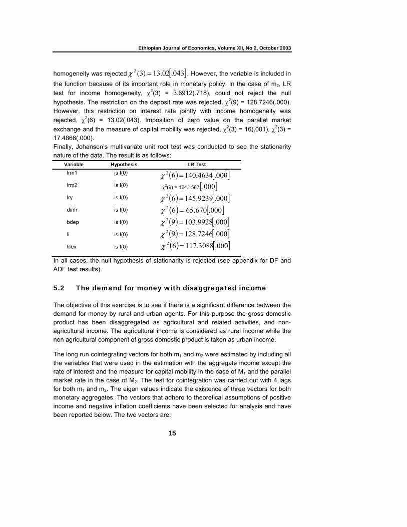
homogeneity was rejected [ ]043.02.13)3(2 =χ . However, the variable is included in the function because of its important role in monetary policy. In the case of m2, LR test for income homogeneity, χ2(3) = 3.6912(.718), could not reject the null hypothesis. The restriction on the deposit rate was rejected, χ2(9) = 128.7246(.000). However, this restriction on interest rate jointly with income homogeneity was rejected, χ2(6) = 13.02(.043). Imposition of zero value on the parallel market exchange and the measure of capital mobility was rejected, χ2(3) = 16(.001), χ2(3) = 17.4866(.000). Finally, Johansen’s multivariate unit root test was conducted to see the stationarity nature of the data. The result is as follows:
Variable Hypothesis LR Test lrm1
lrm2
lry
dinfr
bdep
li
lifex
is I(0)
is I(0)
is I(0)
is I(0)
is I(0)
is I(0)
is I(0)
( ) [ ]000.4634.14062 =χ
χ2(9) = 124.1587 [ ]000.
( ) [ ]000.9239.14562 =χ
( ) [ ]000.670.6562 =χ
( ) [ ]000.9928.10392 =χ
( ) [ ]000.7246.12892 =χ
( ) [ ]000.3088.11762 =χ
In all cases, the null hypothesis of stationarity is rejected (see appendix for DF and ADF test results). 5.2 The demand for money with disaggregated income The objective of this exercise is to see if there is a significant difference between the demand for money by rural and urban agents. For this purpose the gross domestic product has been disaggregated as agricultural and related activities, and non-agricultural income. The agricultural income is considered as rural income while the non agricultural component of gross domestic product is taken as urban income.
The long run cointegrating vectors for both m1 and m2 were estimated by including all the variables that were used in the estimation with the aggregate income except the rate of interest and the measure for capital mobility in the case of M1 and the parallel market rate in the case of M2. The test for cointegration was carried out with 4 lags for both m1 and m2. The eigen values indicate the existence of three vectors for both monetary aggregates. The vectors that adhere to theoretical assumptions of positive income and negative inflation coefficients have been selected for analysis and have been reported below. The two vectors are:
Berhanu Denu: Dynamic money demand function for Ethiopia
16
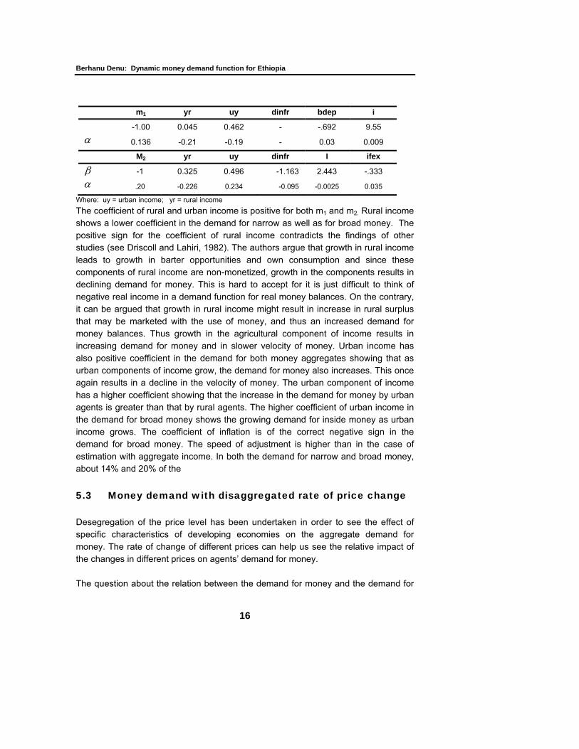
m1 yr uy dinfr bdep i
-1.00 0.045 0.462 - -.692 9.55 α 0.136 -0.21 -0.19 - 0.03 0.009
M2 yr uy dinfr I ifex
β -1 0.325 0.496 -1.163 2.443 -.333 α .20 -0.226 0.234 -0.095 -0.0025 0.035
Where: uy = urban income; yr = rural income The coefficient of rural and urban income is positive for both m1 and m2. Rural income shows a lower coefficient in the demand for narrow as well as for broad money. The positive sign for the coefficient of rural income contradicts the findings of other studies (see Driscoll and Lahiri, 1982). The authors argue that growth in rural income leads to growth in barter opportunities and own consumption and since these components of rural income are non-monetized, growth in the components results in declining demand for money. This is hard to accept for it is just difficult to think of negative real income in a demand function for real money balances. On the contrary, it can be argued that growth in rural income might result in increase in rural surplus that may be marketed with the use of money, and thus an increased demand for money balances. Thus growth in the agricultural component of income results in increasing demand for money and in slower velocity of money. Urban income has also positive coefficient in the demand for both money aggregates showing that as urban components of income grow, the demand for money also increases. This once again results in a decline in the velocity of money. The urban component of income has a higher coefficient showing that the increase in the demand for money by urban agents is greater than that by rural agents. The higher coefficient of urban income in the demand for broad money shows the growing demand for inside money as urban income grows. The coefficient of inflation is of the correct negative sign in the demand for broad money. The speed of adjustment is higher than in the case of estimation with aggregate income. In both the demand for narrow and broad money, about 14% and 20% of the 5.3 Money demand with disaggregated rate of price change Desegregation of the price level has been undertaken in order to see the effect of specific characteristics of developing economies on the aggregate demand for money. The rate of change of different prices can help us see the relative impact of the changes in different prices on agents’ demand for money. The question about the relation between the demand for money and the demand for
Ethiopian Journal of Economics, Volume XII, No 2, October 2003
17
other assets stems from the simple two asset i.e., money- bonds, economy. This simplified approach suggests that agents decide to hold a smaller proportion of their wealth in the form of money as the return on bonds rises. The proportion of income held in the form of bonds increases as the return on bond rises or what amounts to the same thing, as the price of bonds declines. The two-asset approach is based on two assumptions, which are regarded as inadequate. One of the assumptions is that money is regarded as the risk-less asset. The criticism is that short-term securities are also risk free or at least with minimum risk. The other assumption is that change in money stock will also change the prices of risky assets. The criticism here is that many other factors, besides money can result in changing prices of assets. Three alternative approaches to the study of money demand versus the demand for others assets can be identified. First, the money market and term structure approach holds the view that investors prefer to hold short term securities like treasury bills and time deposits in order to hedge against risk. Thus, the demand for money is dependent on income and savings and time deposit rates. Second, the capital market model approach builds its approach on the basis of a linked capital-market system which takes into account the portfolio decisions by businesses, households and the government. The point is that the yield on assets determines the portfolio decision of agents. Third, Brunner and Meltzer approach splits the capital market into three as money market, the debt market and the market for real capital goods, and holds the view that the expenditures for goods and services (it can be the portfolio composition) depends on the relative prices of the assets in the three markets (Mayer, T et al, 1981). From the above brief theoretical background, it can be seen that the portfolio holding of agents depends on the rate of yields on the assets in the portfolio. For empirical study therefore, it is possible to use the rate of change of prices of different goods to see the portfolio effect of change in the demand for money.
Based on the above theoretical background, this study has made an attempt to see the demand for money in Ethiopia within the framework of portfolio choice of agents. For this purpose, the peculiar feature of the Ethiopian economy has been taken into consideration. Ethiopia is mainly an agrarian economy with about 50% of GDP coming from agriculture. Within agriculture, livestock plays a significant role. Livestock ownership is considered as a substitute for capital assets. Also, the holding of deposits in the form of savings and time deposits is limited to an insignificant proportion of the population. Therefore portfolio choice of the Ethiopian agents is between cash and real goods such as cattle, household items, food items, etc. Such a portfolio composition will be affected by changes in the prices of the items. This makes it necessary to study agents’ response to changes in the prices of vitally important assets in the portfolio holdings of agents. Thus, the dis-
Berhanu Denu: Dynamic money demand function for Ethiopia
18
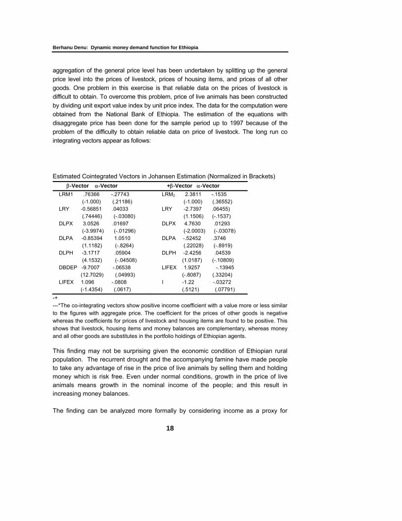
aggregation of the general price level has been undertaken by splitting up the general price level into the prices of livestock, prices of housing items, and prices of all other goods. One problem in this exercise is that reliable data on the prices of livestock is difficult to obtain. To overcome this problem, price of live animals has been constructed by dividing unit export value index by unit price index. The data for the computation were obtained from the National Bank of Ethiopia. The estimation of the equations with disaggregate price has been done for the sample period up to 1997 because of the problem of the difficulty to obtain reliable data on price of livestock. The long run co integrating vectors appear as follows: Estimated Cointegrated Vectors in Johansen Estimation (Normalized in Brackets)
β-Vector α-Vector +β-Vector α-Vector LRM1 .76366 -.27743 (-1.000) (.21186)
LRM2 2.3811 -.1535 (-1.000) (.36552)
LRY -0.56851 .04033 (.74446) (-.03080)
LRY -2.7397 .06455) (1.1506) (-.1537)
DLPX 3.0526 .01697 (-3.9974) (-.01296)
DLPX 4.7630 .01293 (-2.0003) (-.03078)
DLPA -0.85394 1.0510 (1.1182) (-.8264)
DLPA -.52452 .3746 (.22028) (-.8919)
DLPH -3.1717 .05904 (4.1532) (-.04508)
DLPH -2.4256 .04539 (1.0187) (-.10809)
DBDEP -9.7007 -.06538 (12.7029) (.04993)
LIFEX 1.9257 -.13945 (-.8087) (.33204)
LIFEX 1.096 -.0808 (-1.4354) (.0617)
I -1.22 -.03272 (.5121) (.07791)
-+ ---*The co-integrating vectors show positive income coefficient with a value more or less similar to the figures with aggregate price. The coefficient for the prices of other goods is negative whereas the coefficients for prices of livestock and housing items are found to be positive. This shows that livestock, housing items and money balances are complementary, whereas money and all other goods are substitutes in the portfolio holdings of Ethiopian agents. This finding may not be surprising given the economic condition of Ethiopian rural population. The recurrent drought and the accompanying famine have made people to take any advantage of rise in the price of live animals by selling them and holding money which is risk free. Even under normal conditions, growth in the price of live animals means growth in the nominal income of the people; and this result in increasing money balances. The finding can be analyzed more formally by considering income as a proxy for
Ethiopian Journal of Economics, Volume XII, No 2, October 2003
19
wealth (Friedman, 1957). This can be seen from the equation: y = rW or y ÷ r = W, Where y = income, r = a rate of return on wealth, W = wealth A rise in the prices of livestock and housing items is just a rise in the wealth of agents and it results in the growth of income (y). This situation induces a growing demand for real balances. A more plausible for the positive coefficients for the prices of livestock and housing items can be seen from the effect of wealth on money demand. In this regard the demand for real balances can be thought of as a function of real wealth (Harris, 1981). The demand for real balance within such a framework
can be represented by the following equation. ⎟⎟⎠
⎞⎜⎜⎝
⎛+=
rpB
pM
ryfp
M SSD
,
Where: y represents real income, r is an opportunity cost of holding money, Ms and Bs are nominal supply of money and bonds respectively. The money and bonds are assumed as being outside assets and constitute net wealth of the private sector. It is further assumed that the government exogenously determines the supply of nominal money and bonds. Equilibrium in the money and bonds markets can be maintained if the demand for money and bonds is equal to the exogenously determined supply. A change in money balances, ceteris paribus, will result in real balances, which is one component of real wealth. This in turn brings about a shifts in real savings which declines and real investment which grows. Thus an excess demand is created in goods and bonds market while there is excess supply of money. This happens because the model assumes agents to hold a fixed amount of bonds. In the Ethiopian context, since physical assets are being considered rather than bonds, the demand due to wealth effect will be with respect to livestock, housing and housing items. Thus to maintain equilibrium, the prices of these items should rise. This explains the positive coefficients for the prices of livestock and housing and housing items in the demand for money with disaggregated price level in Ethiopia. The coefficient of the other prices is negative as expected. Thus, when prices of other goods increase, agents substitute those goods for money as a hedge against the assets’ rising price. The portfolio effect of price change can be summarized as follows: As the price of livestock rises, people sell them and hold more of their wealth in money form. On the other hand, as the price of all other goods rise, people adjust their portfolio by reducing the money component and increasing the real asset part.
Berhanu Denu: Dynamic money demand function for Ethiopia
20
5.4 The short term demand for narrow money and broad
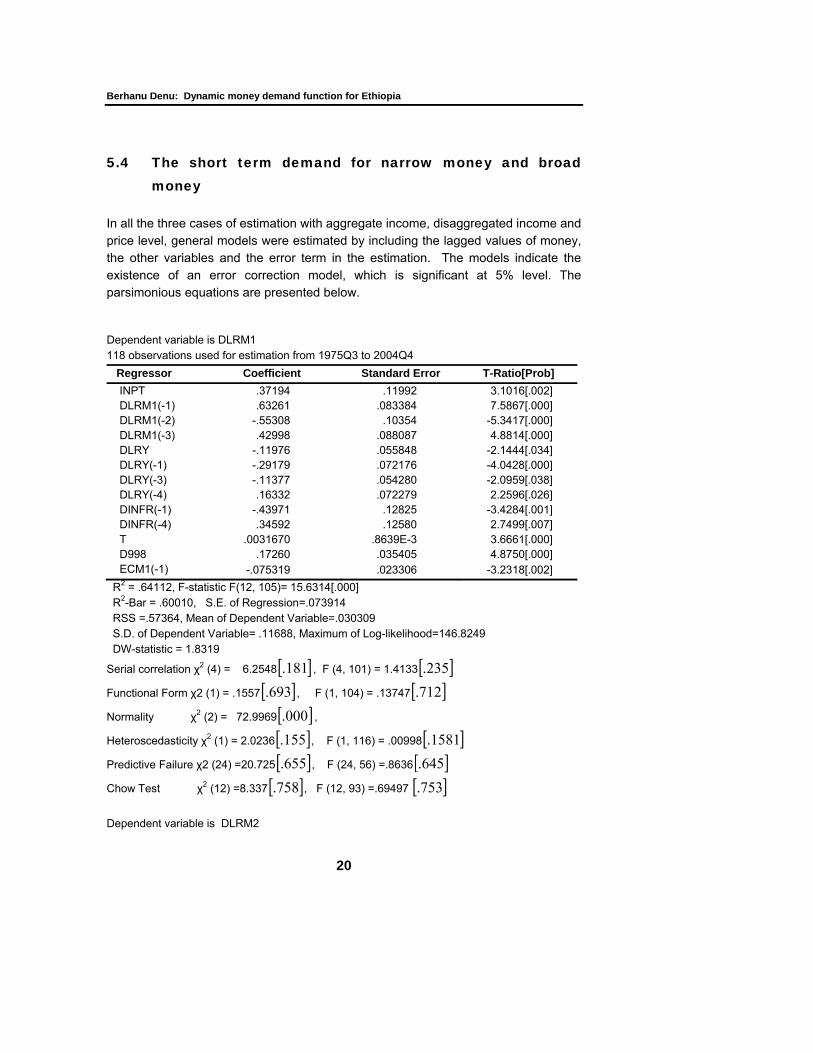
money In all the three cases of estimation with aggregate income, disaggregated income and price level, general models were estimated by including the lagged values of money, the other variables and the error term in the estimation. The models indicate the existence of an error correction model, which is significant at 5% level. The parsimonious equations are presented below. Dependent variable is DLRM1 118 observations used for estimation from 1975Q3 to 2004Q4
Regressor Coefficient Standard Error T-Ratio[Prob] INPT .37194 .11992 3.1016[.002] DLRM1(-1) .63261 .083384 7.5867[.000] DLRM1(-2) -.55308 .10354 -5.3417[.000] DLRM1(-3) .42998 .088087 4.8814[.000] DLRY -.11976 .055848 -2.1444[.034] DLRY(-1) -.29179 .072176 -4.0428[.000] DLRY(-3) -.11377 .054280 -2.0959[.038] DLRY(-4) .16332 .072279 2.2596[.026] DINFR(-1) -.43971 .12825 -3.4284[.001] DINFR(-4) .34592 .12580 2.7499[.007] T .0031670 .8639E-3 3.6661[.000] D998 .17260 .035405 4.8750[.000] ECM1(-1) -.075319 .023306 -3.2318[.002]
R2 = .64112, F-statistic F(12, 105)= 15.6314[.000] R2-Bar = .60010, S.E. of Regression=.073914 RSS =.57364, Mean of Dependent Variable=.030309 S.D. of Dependent Variable= .11688, Maximum of Log-likelihood=146.8249 DW-statistic = 1.8319
Serial correlation χ2 (4) = 6.2548 [ ]181. , F (4, 101) = 1.4133 [ ]235.
Functional Form χ2 (1) = .1557 [ ]693. , F (1, 104) = .13747 [ ]712.
Normality χ2 (2) = 72.9969 [ ]000. ,
Heteroscedasticity χ2 (1) = 2.0236 [ ]155. , F (1, 116) = .00998 [ ]1581.
Predictive Failure χ2 (24) =20.725 [ ]655. , F (24, 56) =.8636 [ ]645.
Chow Test χ2 (12) =8.337 [ ]758. , F (12, 93) =.69497 [ ]753.
Dependent variable is DLRM2

Ethiopian Journal of Economics, Volume XII, No 2, October 2003
21
118 observations used for estimation from 1975Q3 to 2004Q4 Regressor Coefficient Standard Error T-Ratio[Prob] INPT .23622 .037764 6.2552[.000] DINFR -.46304 .069174 -6.6939[.000] DINFR(-2) -.14885 .063774 -2.3340[.021] DLI(-5) -10.7123 3.7078 -2.8891[.005] T .0032193 .4649E-3 6.9249[.000] SC1 -.022358 .010632 -2.1029[.038] D998 .050132 .017963 2.7909[.006] ECM22(-1) -.10735 .016380 -.5538[.000]
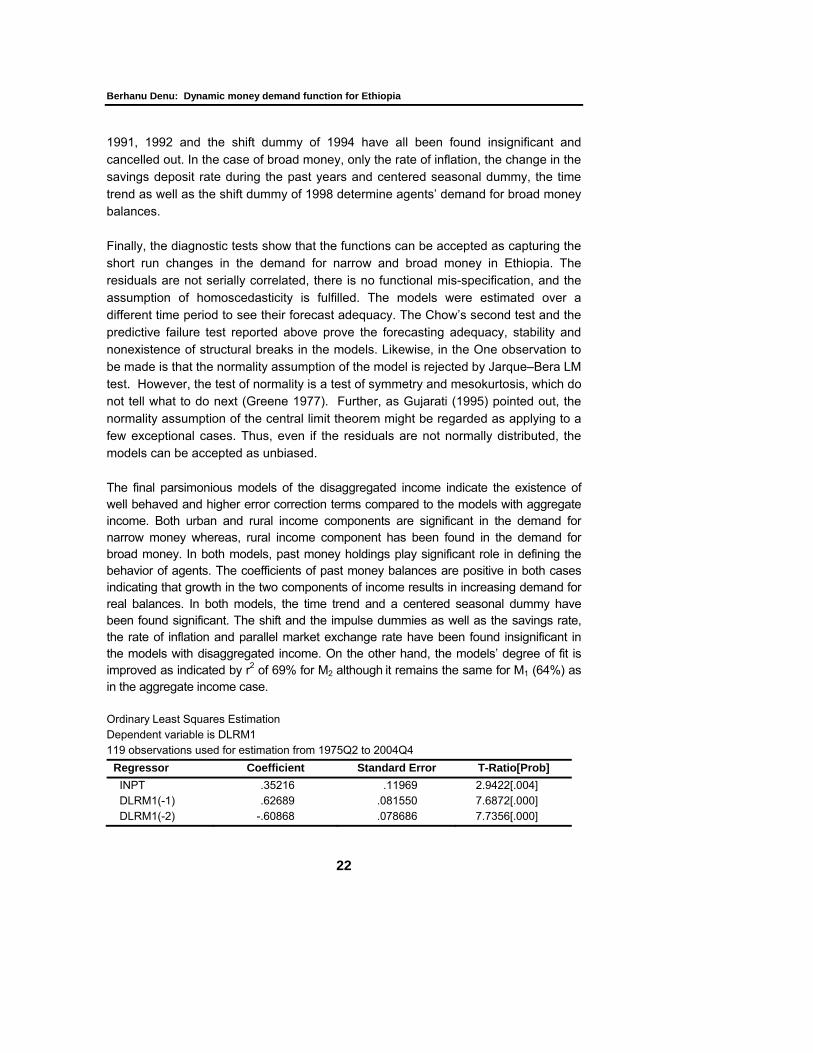
R-Squared .51746 F-statistic F (7, 110) 16.8518[.000] R-Bar-Squared .4878, S.E. of Regression .05 Residual Sum of Squares .27578, Mean of Dependent Variable .018491 S.D. of Dependent Variable .069891, Maximum of Log-likelihood 190.0372 DW-statistic 1.6260, LM = χ2(4)= 3.5335[.473], F (4, 106) =.81804[.516] RESET, χ2(1) = 3.0136[.083], F (1, 109) =2.8567[.094], NORM χ2(2) = 72.2063[.000], Het, χ2(1) = .024870[.875], F (1, 116) = .024453[.876] Predictive Failure χ2(24)=23.8591[.470], F(24, 86)=.99413[.483] Chow Test: χ2(8)= 9.2185[.324],F(8, 102)= 1.1523[.335] The error correction (ecm) term is significant and of the correct sign. However, in both cases, it shows a somewhat lower rate of adjustment and it is about the same size as the value of the α in the long-run vectors. Lagged values of money demand, the rate of inflation, and real income as well as the current level of income significantly affect the demand for narrowly defined real money balances. Also a centered seasonal dummy, the time trend and a shift dummy of 1998 are found significant determinants of the demand for M1. All the coefficients are significant at the 5% level. The income coefficient has a positive sign. Agents increase their real cash balances as their real income rises. The rate of inflation is found to have a rapid and positive impact on the model. Its one period lagged value shows a negative sign. This indicates that agents’ response to the rate of inflation in the immediate past is a reduction of the demand for real balances. On the other hand, the impact of the holdings of money about a year ago, M(1-4), is positive. One possible explanation for such a behavior is that economic agents naturally try to reestablish their real balances, which had been depleted by the higher prices in the preceding period. A more likely cause is that after experiencing inflation in the preceding quarter, agents decide to hold more cash to take advantage in purchasing goods in short of supply whenever the goods become available on the market. The time trend and D998 have positive impact. Agents’ initial response to the uncertainties of financial innovation and policy reform is increased holding of cash balances. The parallel exchange rate, the measure of capital mobility, the impulse dummies of
Berhanu Denu: Dynamic money demand function for Ethiopia
22
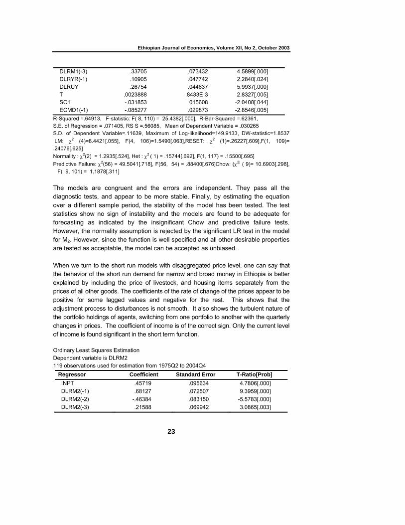
1991, 1992 and the shift dummy of 1994 have all been found insignificant and cancelled out. In the case of broad money, only the rate of inflation, the change in the savings deposit rate during the past years and centered seasonal dummy, the time trend as well as the shift dummy of 1998 determine agents’ demand for broad money balances. Finally, the diagnostic tests show that the functions can be accepted as capturing the short run changes in the demand for narrow and broad money in Ethiopia. The residuals are not serially correlated, there is no functional mis-specification, and the assumption of homoscedasticity is fulfilled. The models were estimated over a different time period to see their forecast adequacy. The Chow’s second test and the predictive failure test reported above prove the forecasting adequacy, stability and nonexistence of structural breaks in the models. Likewise, in the One observation to be made is that the normality assumption of the model is rejected by Jarque–Bera LM test. However, the test of normality is a test of symmetry and mesokurtosis, which do not tell what to do next (Greene 1977). Further, as Gujarati (1995) pointed out, the normality assumption of the central limit theorem might be regarded as applying to a few exceptional cases. Thus, even if the residuals are not normally distributed, the models can be accepted as unbiased. The final parsimonious models of the disaggregated income indicate the existence of well behaved and higher error correction terms compared to the models with aggregate income. Both urban and rural income components are significant in the demand for narrow money whereas, rural income component has been found in the demand for broad money. In both models, past money holdings play significant role in defining the behavior of agents. The coefficients of past money balances are positive in both cases indicating that growth in the two components of income results in increasing demand for real balances. In both models, the time trend and a centered seasonal dummy have been found significant. The shift and the impulse dummies as well as the savings rate, the rate of inflation and parallel market exchange rate have been found insignificant in the models with disaggregated income. On the other hand, the models’ degree of fit is improved as indicated by r2 of 69% for M2 although it remains the same for M1 (64%) as in the aggregate income case. Ordinary Least Squares Estimation Dependent variable is DLRM1 119 observations used for estimation from 1975Q2 to 2004Q4
Regressor Coefficient Standard Error T-Ratio[Prob] INPT .35216 .11969 2.9422[.004] DLRM1(-1) .62689 .081550 7.6872[.000] DLRM1(-2) -.60868 .078686 7.7356[.000]
Ethiopian Journal of Economics, Volume XII, No 2, October 2003
23
DLRM1(-3) .33705 .073432 4.5899[.000] DLRYR(-1) .10905 .047742 2.2840[.024] DLRUY .26754 .044637 5.9937[.000] T .0023888 .8433E-3 2.8327[.005] SC1 -.031853 015608 -2.0408[.044] ECMD1(-1) -.085277 .029873 -2.8546[.005]
R-Squared =.64913, F-statistic: F( 8, 110) = 25.4382[.000], R-Bar-Squared =.62361, S.E. of Regression = .071405, RS S =.56085, Mean of Dependent Variable = .030265 S.D. of Dependent Variable=.11639, Maximum of Log-likelihood=149.9133, DW-statistic=1.8537 LM: χ2 (4)=8.4421[.055], F(4, 106)=1.5490[.063],RESET: χ2 (1)=.26227[.609],F(1, 109)= .24076[.625] Normality : χ2(2) = 1.2935[.524], Het : χ2 ( 1) = .15744[.692], F(1, 117) = .15500[.695] Predictive Failure: χ2(56) = 49.5041[.718], F(56, 54) = .88400[.676]Chow: (χ2) ( 9)= 10.6903[.298], F( 9, 101) = 1.1878[.311] The models are congruent and the errors are independent. They pass all the diagnostic tests, and appear to be more stable. Finally, by estimating the equation over a different sample period, the stability of the model has been tested. The test statistics show no sign of instability and the models are found to be adequate for forecasting as indicated by the insignificant Chow and predictive failure tests. However, the normality assumption is rejected by the significant LR test in the model for M2. However, since the function is well specified and all other desirable properties are tested as acceptable, the model can be accepted as unbiased. When we turn to the short run models with disaggregated price level, one can say that the behavior of the short run demand for narrow and broad money in Ethiopia is better explained by including the price of livestock, and housing items separately from the prices of all other goods. The coefficients of the rate of change of the prices appear to be positive for some lagged values and negative for the rest. This shows that the adjustment process to disturbances is not smooth. It also shows the turbulent nature of the portfolio holdings of agents, switching from one portfolio to another with the quarterly changes in prices. The coefficient of income is of the correct sign. Only the current level of income is found significant in the short term function. Ordinary Least Squares Estimation Dependent variable is DLRM2 119 observations used for estimation from 1975Q2 to 2004Q4
Regressor Coefficient Standard Error T-Ratio[Prob] INPT .45719 .095634 4.7806[.000] DLRM2(-1) .68127 .072507 9.3959[.000] DLRM2(-2) -.46384 .083150 -5.5783[.000] DLRM2(-3) .21588 .069942 3.0865[.003]
Berhanu Denu: Dynamic money demand function for Ethiopia
24
DLRYR .25875 .034396 7.5227[.000] T .0038001 .7876E-3 4.8252[.000] SC1 -.027847 .012850 -2.1671[.032] ECD2(-1) -.12294 .025929 -4.7414[.000]
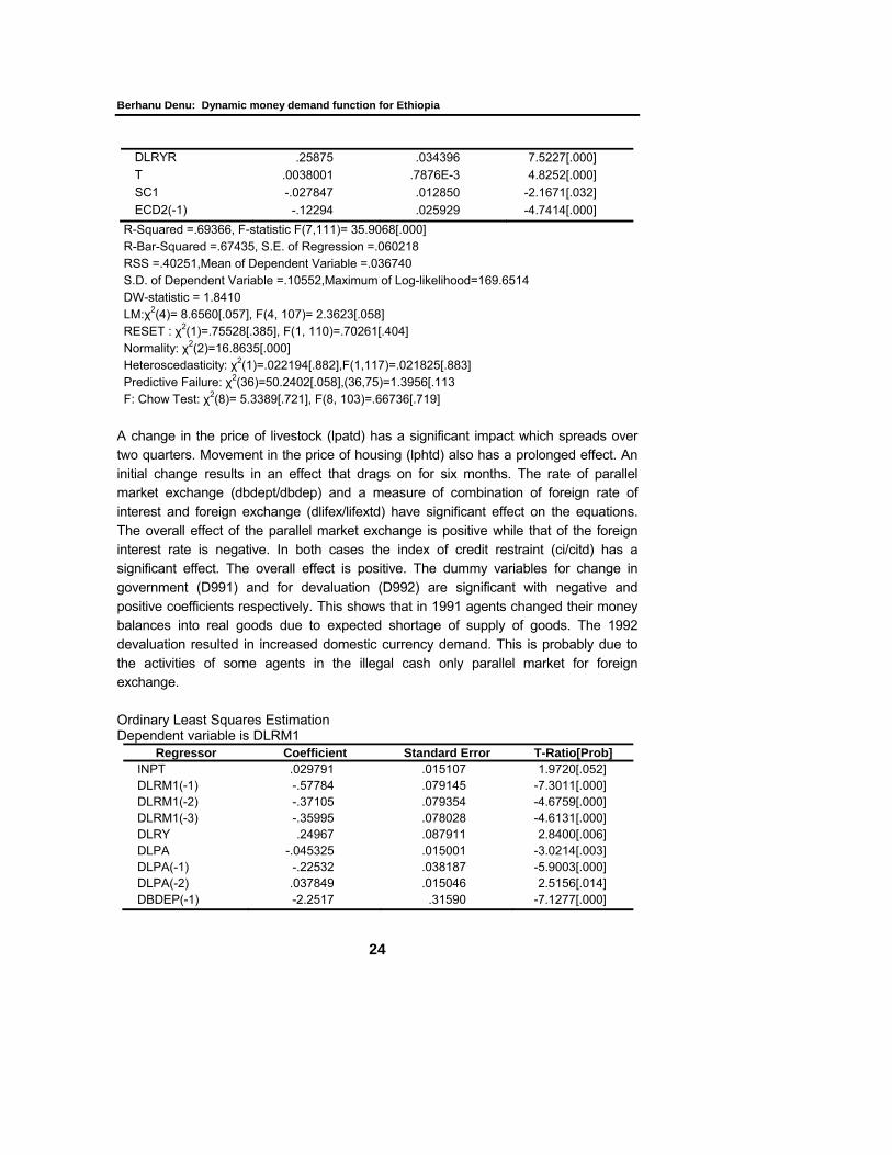
R-Squared =.69366, F-statistic F(7,111)= 35.9068[.000] R-Bar-Squared =.67435, S.E. of Regression =.060218 RSS =.40251,Mean of Dependent Variable =.036740 S.D. of Dependent Variable =.10552,Maximum of Log-likelihood=169.6514 DW-statistic = 1.8410 LM:χ2(4)= 8.6560[.057], F(4, 107)= 2.3623[.058] RESET : χ2(1)=.75528[.385], F(1, 110)=.70261[.404] Normality: χ2(2)=16.8635[.000] Heteroscedasticity: χ2(1)=.022194[.882],F(1,117)=.021825[.883] Predictive Failure: χ2(36)=50.2402[.058],(36,75)=1.3956[.113 F: Chow Test: χ2(8)= 5.3389[.721], F(8, 103)=.66736[.719] A change in the price of livestock (lpatd) has a significant impact which spreads over two quarters. Movement in the price of housing (lphtd) also has a prolonged effect. An initial change results in an effect that drags on for six months. The rate of parallel market exchange (dbdept/dbdep) and a measure of combination of foreign rate of interest and foreign exchange (dlifex/lifextd) have significant effect on the equations. The overall effect of the parallel market exchange is positive while that of the foreign interest rate is negative. In both cases the index of credit restraint (ci/citd) has a significant effect. The overall effect is positive. The dummy variables for change in government (D991) and for devaluation (D992) are significant with negative and positive coefficients respectively. This shows that in 1991 agents changed their money balances into real goods due to expected shortage of supply of goods. The 1992 devaluation resulted in increased domestic currency demand. This is probably due to the activities of some agents in the illegal cash only parallel market for foreign exchange. Ordinary Least Squares Estimation Dependent variable is DLRM1
Regressor Coefficient Standard Error T-Ratio[Prob] INPT .029791 .015107 1.9720[.052] DLRM1(-1) -.57784 .079145 -7.3011[.000] DLRM1(-2) -.37105 .079354 -4.6759[.000] DLRM1(-3) -.35995 .078028 -4.6131[.000] DLRY .24967 .087911 2.8400[.006] DLPA -.045325 .015001 -3.0214[.003] DLPA(-1) -.22532 .038187 -5.9003[.000] DLPA(-2) .037849 .015046 2.5156[.014] DBDEP(-1) -2.2517 .31590 -7.1277[.000]

Ethiopian Journal of Economics, Volume XII, No 2, October 2003
25
DBDEP(-3) 1.1094 .35827 3.0965[.003] DLIFEX -.18860 .087911 -2.1453[.035] DLIFEX(-2) .27748 .098231 2.8248[.006] DLIFEX(-3) -1.1279 .37804 -2.9836[.004] D991 -.12599 .043435 -2.9006[.005] VOLP -.29675 .11967 -2.4798[.015] CI .12397 .018886 6.5642[.000] ECM1D(-1) -.19692 .026537 -7.4207[.000]
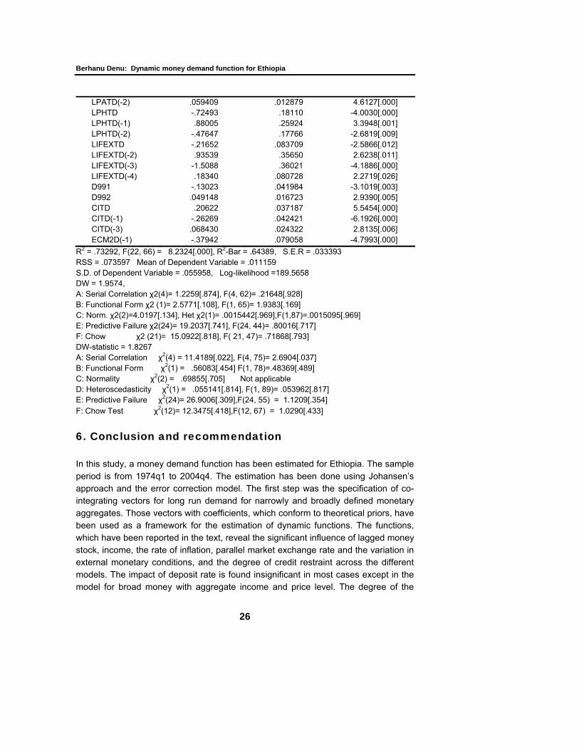
R2 =.69111, F (16, 74) 10.3477[.000] R2-Bar =.62432, S.E. of Regression = .039670 RSS =.11646, Mean of Dependent Variable =.010903 S.D. of Dependent Variable =.064723, Maximum of Log-likelihood = 173.9563 DW = 2.0124, A: Serial Correlation χ2(4)= 3.8499[.427],F(4,70)=.77306[.546] B: Functional Form χ2(1)=.97257[.324], F(1, 73)= .78862[.377] C: Normality χ2(2) = 1.3904[.499] Not applicable D: Heteroscedasticity χ2(1)=.28432[.594], F(1, 89)=.27894[.599] E: Predictive Failure χ2( 24)= 35.9245[.056],F(24, 51)= 1.4969[.113] F: Chow Test χ2 (16)= 21.3288[.166], F( 16, 59)= 1.3331[.209] The measure of price volatility (volp) (for m1) and the error correction term are negatively signed as expected. The figure in both the narrow and broad models, are much higher than the figures with the aggregate models and models with disaggregated income. About 20% of disequilibrium in narrow money demand and about 37% of the disequilibrium in broad money demand is cleared each quarter. The diagnostic tests show no problem in the case of narrow money. Even the problem of normality is solved. However, in the case of the equation for broad money both the LM and F- test showed the presence of serial correlation initially, and the model presented above has been estimated with transformed variables. The transformed variables took the form of X* = Xt- ρXt-1 (J. Durbin, 1960). The transformation has solved the problem of serial correlation. The model has been tested for stability and forecasting adequacy. There is no evidence of instability and predictive inadequacy. The models with disaggregated price level perform better as indicated by higher R2, lower RSS and non violation of the assumption of normality. Ordinary Least Squares Estimation: Dependent variable is M2TD 89 observations used for estimation from 1975Q4 to 1997Q4.
Regressor Coefficient Standard Error T-Ratio[Prob] INPT -.36343 .077418 -4.6945[.000] YTD .48614 .091471 5.3147[.000] LPXTD -.55523 .26378 -2.1049[.039] LPXTD(-1) .72220 .27907 2.5879[.012] DBDEPT(-1) .28790 .098053 2.9362[.005] DBDEPT(-2) -.79115 .32625 -2.4249[.018] DBDEPT(-3) 1.3817 .33904 4.0754[.000] LPATD -.021501 .012552 -1.7129[.091] LPATD(-1) -.053155 .023695 -2.2433[.028]
Berhanu Denu: Dynamic money demand function for Ethiopia
26
LPATD(-2) .059409 .012879 4.6127[.000] LPHTD -.72493 .18110 -4.0030[.000] LPHTD(-1) .88005 .25924 3.3948[.001] LPHTD(-2) -.47647 .17766 -2.6819[.009] LIFEXTD -.21652 .083709 -2.5866[.012] LIFEXTD(-2) .93539 .35650 2.6238[.011] LIFEXTD(-3) -1.5088 .36021 -4.1886[.000] LIFEXTD(-4) .18340 .080728 2.2719[.026] D991 -.13023 .041984 -3.1019[.003] D992 .049148 .016723 2.9390[.005] CITD .20622 .037187 5.5454[.000] CITD(-1) -.26269 .042421 -6.1926[.000] CITD(-3) .068430 .024322 2.8135[.006] ECM2D(-1) -.37942 .079058 -4.7993[.000]
R2 = .73292, F(22, 66) = 8.2324[.000], R2-Bar = .64389, S.E.R = .033393 RSS = .073597 Mean of Dependent Variable = .011159 S.D. of Dependent Variable = .055958, Log-likelihood =189.5658 DW = 1.9574, A: Serial Correlation χ2(4)= 1.2259[.874], F(4, 62)= .21648[.928] B: Functional Form χ2 (1)= 2.5771[.108], F(1, 65)= 1.9383[.169] C: Norm. χ2(2)=4.0197[.134], Het χ2(1)= .0015442[.969],F(1,87)=.0015095[.969] E: Predictive Failure χ2(24)= 19.2037[.741], F(24, 44)= .80016[.717] F: Chow χ2 (21)= 15.0922[.818], F( 21, 47)= .71868[.793] DW-statistic = 1.8267 A: Serial Correlation χ2(4) = 11.4189[.022], F(4, 75)= 2.6904[.037] B: Functional Form χ2(1) = .56083[.454] F(1, 78)=.48369[.489] C: Normality χ2(2) = .69855[.705] Not applicable D: Heteroscedasticity χ2(1) = .055141[.814], F(1, 89)= .053962[.817] E: Predictive Failure χ2(24)= 26.9006[.309],F(24, 55) = 1.1209[.354] F: Chow Test χ2(12)= 12.3475[.418],F(12, 67) = 1.0290[.433]
6. Conclusion and recommendation In this study, a money demand function has been estimated for Ethiopia. The sample period is from 1974q1 to 2004q4. The estimation has been done using Johansen’s approach and the error correction model. The first step was the specification of co-integrating vectors for long run demand for narrowly and broadly defined monetary aggregates. Those vectors with coefficients, which conform to theoretical priors, have been used as a framework for the estimation of dynamic functions. The functions, which have been reported in the text, reveal the significant influence of lagged money stock, income, the rate of inflation, parallel market exchange rate and the variation in external monetary conditions, and the degree of credit restraint across the different models. The impact of deposit rate is found insignificant in most cases except in the model for broad money with aggregate income and price level. The degree of the
Ethiopian Journal of Economics, Volume XII, No 2, October 2003
27
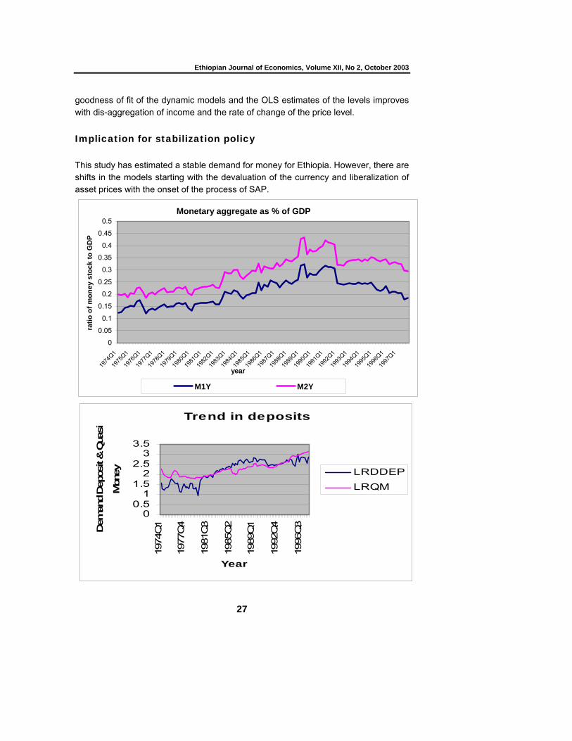
goodness of fit of the dynamic models and the OLS estimates of the levels improves with dis-aggregation of income and the rate of change of the price level. Implication for stabilization policy This study has estimated a stable demand for money for Ethiopia. However, there are shifts in the models starting with the devaluation of the currency and liberalization of asset prices with the onset of the process of SAP.
Monetary aggregate as % of GDP
0
0.05
0.1
0.15
0.2
0.25
0.3
0.35
0.4
0.45
0.5
1974
Q1
1975
Q1
1976
Q1
1977
Q1
1978
Q1
1979
Q1
1980
Q1
1981
Q1
1982
Q1
1983
Q1
1984
Q1
1985
Q1
1986
Q1
1987
Q1
1988
Q1
1989
Q1
1990
Q1
1991
Q1
1992
Q1
1993
Q1
1994
Q1
1995
Q1
1996
Q1
1997
Q1
year
ratio
of m
oney
sto
ck to
GD
P
M1Y M2Y
Trend in deposits
00.5
11.5
22.5
33.5
1974
Q1
1977
Q4
1981
Q3
1985
Q2
1989
Q1
1992
Q4
1996
Q3
Year
Dem
and
Dep
osit
& Q
uasi
Mon
ey LRDDEP
LRQM
Berhanu Denu: Dynamic money demand function for Ethiopia
28
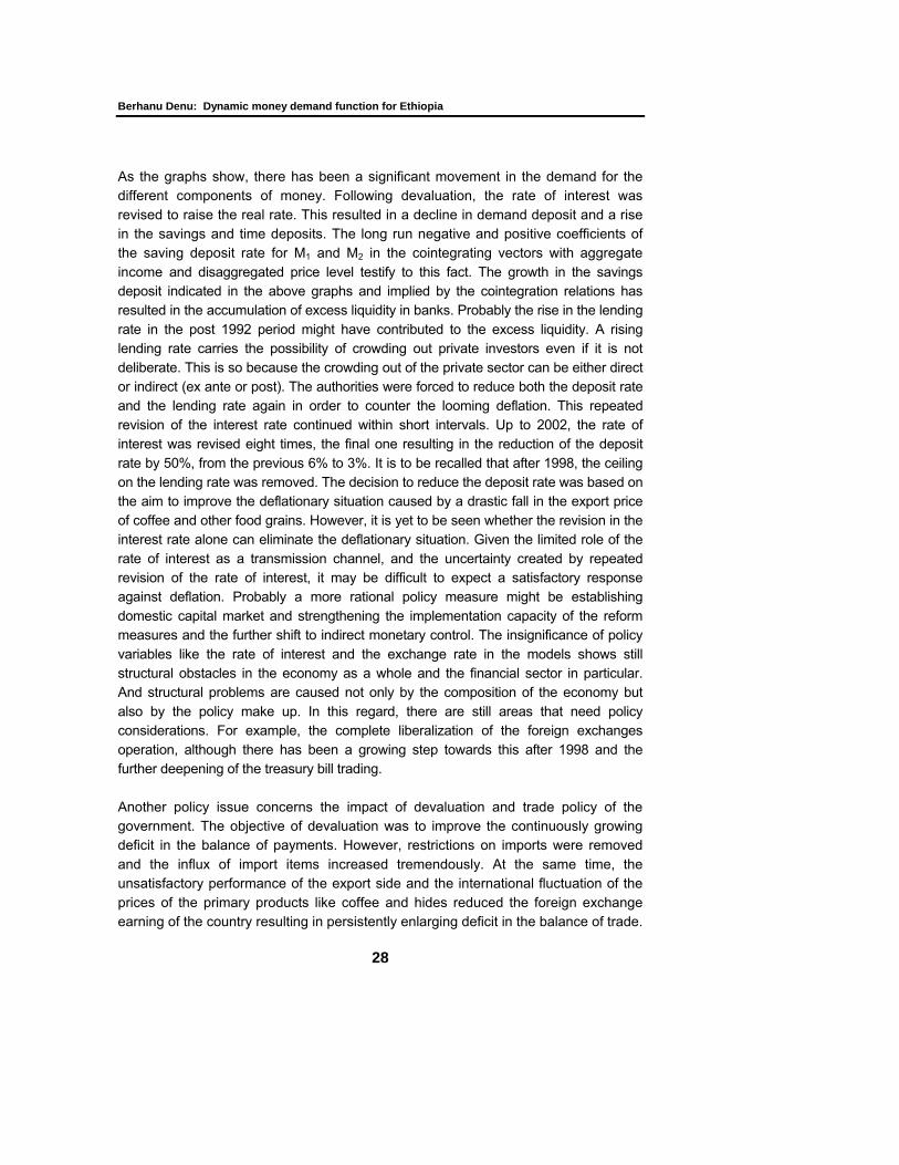
As the graphs show, there has been a significant movement in the demand for the different components of money. Following devaluation, the rate of interest was revised to raise the real rate. This resulted in a decline in demand deposit and a rise in the savings and time deposits. The long run negative and positive coefficients of the saving deposit rate for M1 and M2 in the cointegrating vectors with aggregate income and disaggregated price level testify to this fact. The growth in the savings deposit indicated in the above graphs and implied by the cointegration relations has resulted in the accumulation of excess liquidity in banks. Probably the rise in the lending rate in the post 1992 period might have contributed to the excess liquidity. A rising lending rate carries the possibility of crowding out private investors even if it is not deliberate. This is so because the crowding out of the private sector can be either direct or indirect (ex ante or post). The authorities were forced to reduce both the deposit rate and the lending rate again in order to counter the looming deflation. This repeated revision of the interest rate continued within short intervals. Up to 2002, the rate of interest was revised eight times, the final one resulting in the reduction of the deposit rate by 50%, from the previous 6% to 3%. It is to be recalled that after 1998, the ceiling on the lending rate was removed. The decision to reduce the deposit rate was based on the aim to improve the deflationary situation caused by a drastic fall in the export price of coffee and other food grains. However, it is yet to be seen whether the revision in the interest rate alone can eliminate the deflationary situation. Given the limited role of the rate of interest as a transmission channel, and the uncertainty created by repeated revision of the rate of interest, it may be difficult to expect a satisfactory response against deflation. Probably a more rational policy measure might be establishing domestic capital market and strengthening the implementation capacity of the reform measures and the further shift to indirect monetary control. The insignificance of policy variables like the rate of interest and the exchange rate in the models shows still structural obstacles in the economy as a whole and the financial sector in particular. And structural problems are caused not only by the composition of the economy but also by the policy make up. In this regard, there are still areas that need policy considerations. For example, the complete liberalization of the foreign exchanges operation, although there has been a growing step towards this after 1998 and the further deepening of the treasury bill trading. Another policy issue concerns the impact of devaluation and trade policy of the government. The objective of devaluation was to improve the continuously growing deficit in the balance of payments. However, restrictions on imports were removed and the influx of import items increased tremendously. At the same time, the unsatisfactory performance of the export side and the international fluctuation of the prices of the primary products like coffee and hides reduced the foreign exchange earning of the country resulting in persistently enlarging deficit in the balance of trade.
Ethiopian Journal of Economics, Volume XII, No 2, October 2003
29
Furthermore, it also seems possible that the growing demand for money in the post devaluation period might have been used in conducting the illegal trade that had become so rampant in the aftermath of political turbulence. The massive resort to illegal cross border trade has greatly harmed the officially licensed businesses. Unable to withstand the almost dumping prices of the illegal traders, a number of businesses have been force to close down. The ever-expanding illegal trade has also a negative impact on government revenue in two ways. First, the illegal traders do not pay any tax since they are not legally registered. Second, the unlawful competition from the illegal businesses has reduced the earnings of the lawful businesses thereby resulting in reduced tax paid to the government. The low revenue base is probably the major cause for growing fiscal deficit. The government has been tackling the problem of the deficit budget with the receipt from the sale of Treasury bill and external and internal borrowing. The auctioning of the Treasury bill was started with the aim of developing the inter-bank secondary market. However, this objective was defeated for the banks used their excess liquidity solely for the trade in the Treasury bill. Again a more rational policy might be the adoption of measures that may facilitate the development of secondary markets and strengthen the measures of indirect control. The government also needs to put in place a sound trade policy, which will balance between the liberalization of imports and the protection of domestic production. It must be kept in mind that liberalization of trade should take into account the specific conditions of countries. Boots of the correct size and quality are needed. Another point of policy concern is the low (0.045)/0.3) coefficient for rural income showing that growth in rural income results in a modest demand for money. The explanation is that growth in rural income results in the growth of own consumption and non-monetized components of income thereby creating discrepancy between the growth in income and the growth in the demand for money. This tendency of a slow growth in the demand for money in rural areas must be countered with exchange oriented rural development policy. This demands, among other things, the expansion of off-farm activities and small-scale rural industries, which can serve as a bridge to integrate the rural and the urban areas. It seems more plausible to accept the view that the use of money and the development of exchange with money can bring about the desired improvement in the life of the rural population. Furthermore, a policy that creates a sound marketing facility for livestock, especially in the pastoral areas, is needed. The pastoral areas lose a lot as a result of illegal cross border trade in livestock. The creation of better marketing for other agricultural products is also of paramount importance. The recent experience in the country with the crisis caused due to inability of the rural population to sell surplus food grains is a signal for the Agricultural-led-development strategy about what is in stock for unbalanced growth

Berhanu Denu: Dynamic money demand function for Ethiopia
30
between agriculture and other sectors. Thus while it may be necessary to give greater emphasis to an accelerated development of agriculture, it is equally necessary to give emphasis to the growth and development of other sectors. One of the findings is that the rate of inflation plays a significant role in shaping the short run behavior of agents. Hence the authorities have been targeting inflation to ensure macroeconomic stability. The authorities have been targeting inflation to a single digit rate. This has been so in accordance with the IMF principles of Enhanced Structural Adjustment Facility (ESAF prior to 1999) and Growth and Poverty Reduction Facility (GPRF since 1999). The average rate of inflation has been on average about 4% to 6 % between 1997 and 2003/2004. This seems to be partly the result of the decline in the prices of food grains as a result of good harvest due to favorable weather condition during part of the sample period. On the other hand, the government’s commitment to tight fiscal and monetary policy as per the agreement with the IMF, has also limited the rate of inflation to the single digit low level. However, it is questionable whether the policy of the single digit inflation rate can result in accelerated growth as it has been expected. There are empirical studies, some of them by economists within the IMF, which indicate higher thresholds for developing countries (Khan, S). Such studies report different thresholds for developed and developing countries. The thresholds are lower for industrialized economies than for the developing economies. Khan reports that the positive effect of inflation on growth is below a 5% rate whereas it ranges up to 18% of inflation for the developing countries. Further, the present study gives about a 10% revenue maximizing rate of inflation. Thus, the authorities should negotiate for a rate of inflation of about 10% for growth to pick up from the present low level. Under the GPRF agreement, the government’s borrowing from domestic banks has been limited to a mere one billion birr and monetary expansion has been further curbed by strictly observing the situation in the credit to the private sector. External borrowing is to be limited mainly to concessional loans. The demand for m2 has increased as a result of growth in all the components of deposit. There is also a build up in excess liquidity of banks partly due to a decline in the demand for credit. It seems that the achievement of macroeconomic stability is associated with the undesirable deflationary situation. The attainment of macroeconomic stability is a necessary policy objective. However, it is only one aspect of economic reform programs. The other equally important aspect is growth and development of the economy. There cannot be a sustainable stability without growth that can improve the life of the people. The trend in growth reported over the past couple of years should be complemented with policies that further strengthen the participation of the private sector. Another important policy relevant finding of the study is the effect of the measure of capital mobility shown in the long run equations. A gap between domestic and foreign interest rates and exchange rate induces domestic agents’ demand for foreign
Ethiopian Journal of Economics, Volume XII, No 2, October 2003
31
assets. The measure of capital mobility has a significant negative coefficient. This shows the necessity to give due consideration to international monetary policy in the formulation of domestic policy. In sum, the econometric result from this study shows the existence of stable long run and dynamic money demand function for Ethiopia despite liberalization measures after 1992. However, there has been some adjustment in the asset portfolio holding of the private agents. But the preference for liquidity is still high showing slower response of agents to structural adjustment. A more rigorous policy that strengthens the process of privatization and a faster move towards more indirect control can be more rational to pursue. It is also of paramount importance to give due consideration to external monetary and financial development in the formulation of domestic stabilization policy.
Berhanu Denu: Dynamic money demand function for Ethiopia
32
References Adam, C. (1992). On the Dynamic Specification of Money Demand in Kenya, Journal of African
Economies, vol. 1, 2, pp. 233-270. ______. (1999). Financial Liberalization and Currency Demand in Zambia, Journal of African
Economies, 8(3): 268-306. Agenor, P. R. and M. S. Khan. (1996). Foreign Currency Deposits and Demand for Money in
Developing Countries”, Journal of Development Economics, Vol. 50, pp. 101-118. Arango, Sebastian and Ishag M. Nadiri. (1981). Demand for Money in Open Economies,
Journal of Monetary Economics, Vol. 7, January, PP. 69-83. Arize, A. C., Malindretos, J. and Christofferson, S. (2003). Monetary Dynamics, Exchange
Rates and Parameter Stability: AN Empirical Investigation, Journal of Economic Studies, 30, No.5, pp. 493-573.
Arize, A. C. and Ghosh, D. (2003). Profit Possibilities in Currency Markets: Arbitrage, Hedging and Speculation, The Financial Review, 38. pp. 473-496.
Arize, A. C., Malindretos, J. and S. S. Shwiff. (1999). Structural Breaks, Cointegration, and Speed of Adjustment: Evidence From 12 LDCs Money Demand, International Review of Economics and Finance, 8, pp. 399-420.
Arize, A. C. and Shwiff, S. S. (1998). The Appropriate Exchange-rate Variable in the Money Demand of 25 Countries: An Empirical Investigation, North American Journal of Economics and Finance, 9, pp. 169-185.
Arize, Augustine C. (1989), An Econometric Investigation of Money Demand Behavior in Four Asian Developing Economies, International Economic Journal, Vol. 3, pp. 79-93.
Atingi-Ego, M. and Matthew, K. A. (1996). Demand for Narrow Money and Broad Money in Uganda, The Journal of African Review of Money, Finance and Banking, issue No. 1/96
______. (1996). Financial Deregulation and Its Implications for the Micro-economy (unpublished), PhD Thesis, September 1996, Liverpool Business School, JMU.
Bahmani-Oskoee, M. Pourheydarian, (1990). Exchange Rate Sensitivity of the Demand for Money and Effectiveness of the Fiscal and Monetary Policies, Applied Economics, Vol. 22, pp. 917-925.
Bahmani-Oskooee, Mohsen. (1996). The Black Market Exchange Rate and Demand for Money in Iran, Journal of Macroeconomics, Vol. 18 (Winter), pp.171-76.
Baumol, W. J. (1952). The Transaction Demand For Cash: An Inventory Theoretic Approach, reprinted in Richard S. Thorn (ed.), Monetary Theory and Policy.
Charlanbides, N. (1992). Demand for Money and Disagrregation of Income in Kenya, Unpublished. PhD Dissertation.
Central Statistical Office (Addis Ababa). (1990). Statistical Abstract,. Choudhry, T. A. (1995). Long run Money Demand Function in Argentina during 1935-1962:
Evidence from Cointegration and Error Correction Models, Applied Economics, 27, 661-667. Darrat, A. F. (1986). Money, Inflation and Causality in the North African Countries, Journal of
Macroeconomics, Vol. 8, pp 87-103. Dickey, D. A. and Fuller, W. A. (1979). A Distribution of The Estimators for Auto Regressive Time
Series with a Unit Root, Journal of the American Statistical Association, vol. 47, pp.427-31. Domowitz, I .and Elbadawi, I. (1987). An Error Correction Approach to Money Demand: The
Case of Sudan, Journal of Development Economics, 26 (1987), 257- 275. Doornik J. A., D. F. Hendry and B. Nielson. (1998). Inference in co integrated models: UK M1
revisited, Journal of Economic Surveys, Vol. 12 (5) 533-572.
Ethiopian Journal of Economics, Volume XII, No 2, October 2003
33
Driscoll, M. J., and A. K. Lahiri. (1983). Income Velocity of Money in Agricultural Developing Economies, Review of Economics and Statistics, 65, pp. 393-401.
Durbin, J. (1960). Estimation of Parameters in Time Series Regression Models, Journal of the Royal Statistical Society, August 1983, pp. 139-153.
Ergete A. (1998). An Error Correction Approach to Money Demand: The Case of Ethiopia, unpublished MSC Thesis, School of Graduate Studies, Addis Ababa University
Engle, R. F. and Granger, C. W. J. (1987). A Cointegration and Error Correction: Representation, Estimation and Testing, Econometria, Vol. 55, 2 March 1987, pp. 251-276.
Fielding, D. (1993). On the Dynamic Specification of Money Demand in Cameroon, Nigeria, Cote D’Ivoire and Kenya, Credit Research paper No. 93/8.
Fisher, D. (1978). Monetary Theory and Demand for Money London: Martin Robertson & Co. Ltd. Friedman, B. M. (1956). The Quantity Theory of Money: A Restatement, in Richard, S Thorn,
opcit. _____. (1959). The Demand for Money: Some Theoretical and Empirical Results, in Richard, S.
Thorn (ed.) opcit. Ghatak, Subrata. (1981). Monetary Economics in developing countries, London, Macmillan Goldstein, M. and M. Khan. (1976). Large Versus Small Price Changes and the Demand for
Imports, IMF Staff Papers, 200-223. Grandmont, J. M. (1985). Money and Value: A Reconsideration of Classical and Neo-classical
Monetary Theories, An Econometric Society, London: Cambridge University Press. Green, W. H. (1997). Econometric Analysis, Third Ed.., New York, Macmillan. Gujarati, Damodar. (1968). The Demand for Money In India, the Journal of Development
Studies, Vol. 5, pp. 59-64. _____ (1995), Basic Econometrics, Third Ed.., New York, McGraw-Hill. Gupta, K. L. (1970). The Demand for Money in India: Further Evidence, The Journal of
Development Studies, pp.159-68. Hendry, D. F. and Ericsson, N. R. (1990). Modeling the Demand for Narrow Money In the United
Kingdom and The United States, European Economic Review, Vol. 35, pp. 833-86. Hoffman, D.L. and Tahiri, C. (1994). Money Demand in Morocco: Estimating Lon-run Elasticity
for a Developing Country, Oxford Bulletin of Economics and Statistics 56, 3 (1994), pp.305-323
Holden, K. (1995). Vector Auto-regression Modeling and Forecasting, Journal of Forecasting, May 1995.
Ibrahim, S. B. and Kumah, F. Y. (1996). Co movements in Budget Deficits, Money, Interest Rates, Exchange Rates, and the Current Account Balance: Some Empirical Evidence, Journal of Applied Economics, 28, 117-130
Ireland, P. N. (1995). Endogenous Financial Innovation and the Demand for Money, Journal of Money, Credit and Banking 27, 1 (1995), pp.107-123.
Johansen, S. (1988). A Statistical Analysis of Cointegration Vectors, Journal of Economic Dynamics and Control, as reprinted in Engle and Granger (1991)
Johansen, S. and Jusilius, K, (1990). A Maximum Likelihood Estimation- With Applications to the Demand for Money, Oxford Bulletin of Economics and Statistics 52, 2 (1990) pp. 169-210.
Kennedy, P. (1979). A Guide to Econometrics, Third Ed. Oxford: Blackwell Publishers Ltd. Keynes, J. M. (1930). Treatise on Money in Vol. 2, the Applied Theory of Money, Macmillan. Khan, S. M. (2002). Inflation, Financial Deepening and Economic Growth: Paper presented for
the Banco de Mexico Conference on Macroeconomic Stability, Financial Markets and Economic Growth, Mexico City, November 2002, 12-13,.
Klovland, J. T. (1987). The Demand for Money in the United Kingdom: 1875- 1913”, Oxford Bulletin of Economics and Statistics 49, 3 (1987) pp. 251- 271.
Berhanu Denu: Dynamic money demand function for Ethiopia
34
Laidler, D. E. W. (1977). Demand for Money:: Theories and Evidence, Second ed. Dun Donnelley
Laumas, P. S. (1978). Monetization, Economic Development and the Demand for Money, Review of Economics and Statistics, 60, pp. 614-618.
Lulseged A. (1996). Money Demand and Monetization in Ethiopia, Unpublished MSc Thesis, School of Graduate Studies, Addis Ababa University.
McKinnon, R. I. (1982). Currency Substitution and Instability in the World Dollar Standard, American Economic Review, Vol. 72, pp. 320-333.
Marx, K. (1970). Capital:, A critical Analysis of Capitalist Production 3 Vol., Progress Publisher. Mayer, T. et al. (1981). Money, Banking and the Economy, New York, W. W. Norton. Melink, Rafi. (1995). Financial Services, Cointegration and the Demand for Money in Israel”,
Journal of Money, Credit and Banking Vol. 27, 1 pp. 140-153 Miller, S. M. (1991). Monetary Dynamics: An application of Cointegration and Error Correction
Modeling, Journal of Money, Credit and Banking 23, 2 (1991) pp. 139-154 Murindi, Victor. (1996). Development Banking and Finance, Ashgate Publishing Ltd. National Bank of Ethiopia (NBE). (1983, 1990, 1992). Annual Report. Patinkin, D. (1965). A Critique of Neo-classical Monetary Theory as reprinted in Richard S
Thorn, opcit. Peseran and Peseran. (1987). Microfit Users Guide. Pilbeam, K. (1992). International Finance, Macmillan. Plosser, Charles I., Shwert, G. W. and White, H. (1982). “Differencing A S A Test of Specification”,
International Economic Review, Vol. 23, No. 3,( October,1982), pp. 535-553. Pokorny, M. (1987). An Introduction to Econometrics, Oxford: Blackwell publishers. Psaradakis,
Z. The Demand for money in Greece: An Exercise in Econometric Modeling with Cointegrated Variables Oxford Bulletin of Economics and statistics 55, 2(1993), pp. 214-234
Randa, J. (1999). The Demand for Money in Tanzania, Journal of African Economies, 8(3): 307-44. Samuel Mulugeta Badwaza. (2005). The Demand for Money and Monetary Policy in Ethiopia
unpublished MSc Thesis, School of Graduate Studies, Addis Ababa University Sidrauski, M (1967b). Rational Choice and Patterns of Growth in a Monetary Economy’,
American Economic Association Papers and Proceedings, Vol. 57, pp.534-544. Simons, R. (1992). An Error Correction Approach to Demand for Money in Five African
Developing Countries, Journal of Economic Studies 19, 1(1992) PP. 29-47. Siriram, Subramanian S. (2001). A Survey of Recent Empirical Money Demand Studies, IMF
Staff Papers, Vol. 47(3), pp.334-365. Sterken, E. (1999). Demand for Money and Shortage in Ethiopia, Centre for Development Studies,
University of Groningen, Research Report No. 199909, Groningen, Netherlands. Tobin, J. (1958). A Liquidity Preference as Behavior towards Risk” Review of Economic
Studies, as in Richard S Thorn (ed.) opcit. ______. (1965c). The Theory of Portfolio Selection in F. H. Hahn and F. P. R. Brechling (eds.)
The Theory of Interest Rates, London , Macmillan Villanueva, D. and A. Mirakhor. (1990). Strategies for Financial Reforms: Interest rate Policies,
Stabilization and Bank Supervision in Developing Countries, IMF Staff Papers, vol. 37.3.
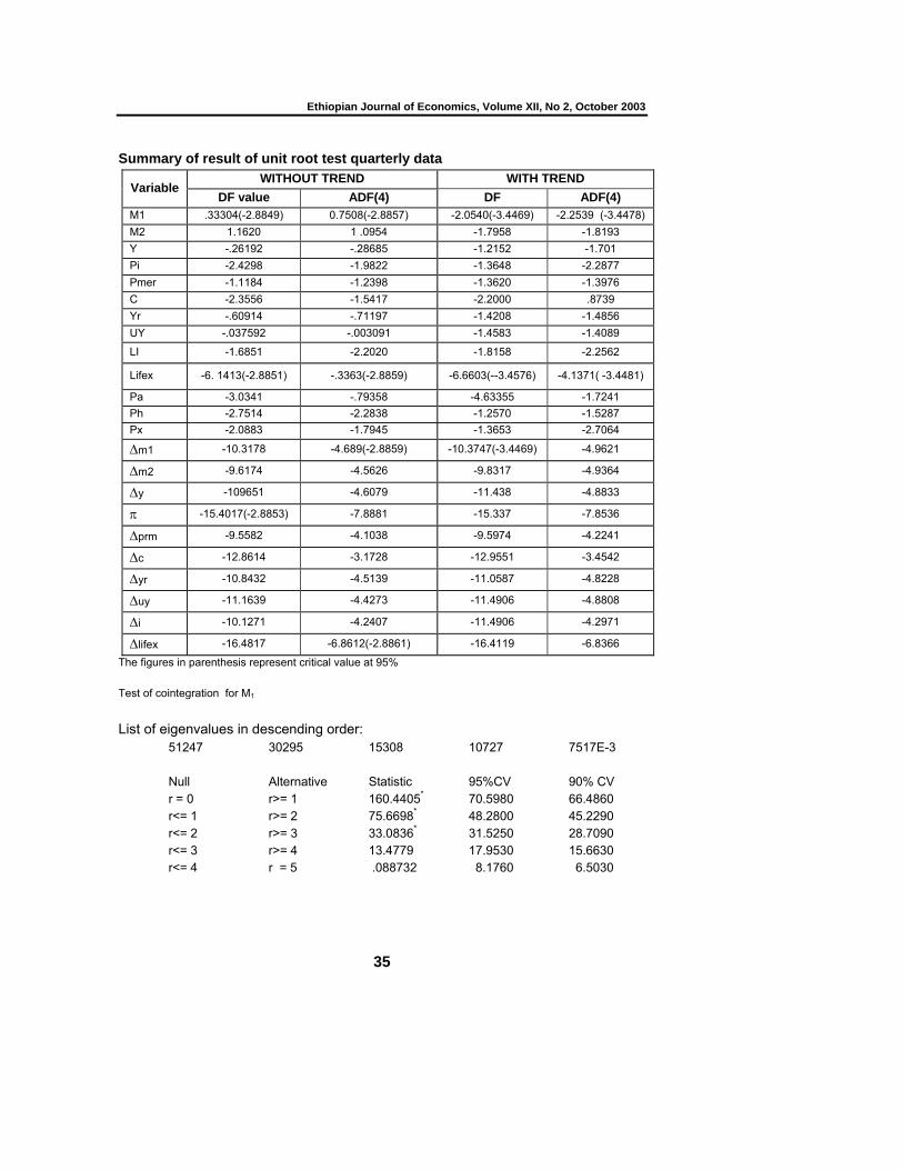
Ethiopian Journal of Economics, Volume XII, No 2, October 2003
35
Summary of result of unit root test quarterly data
Variable WITHOUT TREND WITH TREND
DF value ADF(4) DF ADF(4) M1 .33304(-2.8849) 0.7508(-2.8857) -2.0540(-3.4469) -2.2539 (-3.4478) M2 1.1620 1 .0954 -1.7958 -1.8193 Y -.26192 -.28685 -1.2152 -1.701 Pi -2.4298 -1.9822 -1.3648 -2.2877 Pmer -1.1184 -1.2398 -1.3620 -1.3976 C -2.3556 -1.5417 -2.2000 .8739 Yr -.60914 -.71197 -1.4208 -1.4856 UY -.037592 -.003091 -1.4583 -1.4089
LI -1.6851 -2.2020 -1.8158 -2.2562
Lifex -6. 1413(-2.8851) -.3363(-2.8859) -6.6603(--3.4576) -4.1371( -3.4481)
Pa -3.0341 -.79358 -4.63355 -1.7241 Ph -2.7514 -2.2838 -1.2570 -1.5287 Px -2.0883 -1.7945 -1.3653 -2.7064
∆m1 -10.3178 -4.689(-2.8859) -10.3747(-3.4469) -4.9621
∆m2 -9.6174 -4.5626 -9.8317 -4.9364
∆y -109651 -4.6079 -11.438 -4.8833
π -15.4017(-2.8853) -7.8881 -15.337 -7.8536
∆prm -9.5582 -4.1038 -9.5974 -4.2241
∆c -12.8614 -3.1728 -12.9551 -3.4542
∆yr -10.8432 -4.5139 -11.0587 -4.8228
∆uy -11.1639 -4.4273 -11.4906 -4.8808
∆i -10.1271 -4.2407 -11.4906 -4.2971
∆lifex -16.4817 -6.8612(-2.8861) -16.4119 -6.8366
The figures in parenthesis represent critical value at 95% Test of cointegration for M1 List of eigenvalues in descending order:
51247 30295 15308 10727 7517E-3 Null Alternative Statistic 95%CV 90% CV r = 0 r>= 1 160.4405* 70.5980 66.4860 r<= 1 r>= 2 75.6698* 48.2800 45.2290 r<= 2 r>= 3 33.0836* 31.5250 28.7090 r<= 3 r>= 4 13.4779 17.9530 15.6630 r<= 4 r = 5 .088732 8.1760 6.5030
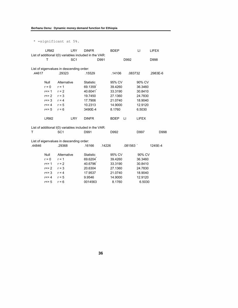
Berhanu Denu: Dynamic money demand function for Ethiopia
36
* =significant at 5%. LRM2 LRY DINFR BDEP LI LIFEX
List of additional I(0) variables included in the VAR: T SC1 D991 D992 D998
List of eigenvalues in descending order: .44617 .29323 .15529 .14106 .083732 .2983E-6
Null Alternative Statistic 95% CV 90% CV r = 0 r = 1 69.1359* 39.4260 36.3460 r<= 1 r = 2 40.6041* 33.3190 30.8410 r<= 2 r = 3 19.7450 27.1360 24.7830 r<= 3 r = 4 17.7906 21.0740 18.9040 r<= 4 r = 5 10.2313 14.9000 12.9120 r<= 5 r = 6 3490E-4 8.1760 6.5030
LRM2 LRY DINFR BDEP LI LIFEX
List of additional I(0) variables included in the VAR: T SC1 D991 D992 D997 D998 List of eigenvalues in descending order: .44846 .29368 .16166 .14226 .081563 1245E-4
Null Alternative Statistic 95% CV 90% CV r = 0 r = 1 69.6204* 39.4260 36.3460 r<= 1 r = 2 40.6796* 33.3190 30.8410 r<= 2 r = 3 20.6304 27.1360 24.7830 r<= 3 r = 4 17.9537 21.0740 18.9040 r<= 4 r = 5 9.9546 14.9000 12.9120 r<= 5 r = 6 0014563 8.1760 6.5030

Ethiopian Journal of Economics, Volume XII, No 2, October 2003
37
Related Documents