Dynamic labour force participation of married women in Sweden

Dynamic labor force participation of married women in Sweden

Nizamul Islam∗

Abstract: This paper analyzes the inter-temporal labor force participation behavior of married women in

Sweden. A dynamic probit model is applied, controlling for endogenous initial condition and unobserved

heterogeneity, using longitudinal data to allow for a rich dynamic structure. Significant unobserved

heterogeneity is found, along with serial correlation in the error components, and negative state

dependence. The findings may indicate serial persistence due to persistent individual heterogeneity.

Keywords: Inter-temporal labor force participation, state dependence, heterogeneity. JEL: J22, C23, C25

∗ Department of Economics, Göteborg University, Sweden E-mail: [email protected] February 18, 2005

1

1 Introduction

Individuals who have experienced unemployment are more likely to experience same event

in the future. Heckman (1981) shows two explanation of this serial persistence. The first

one is “true state dependence” in which current participation depends on past participation.

And the second is “spurious state dependence” in which an individual component

determines current participation irrespective of past participation. However, these two

sources of persistence in individual participation decisions have very different implications,

for example, in evaluating the effect of economic policies that aim to alleviate short-term

unemployment (e.g., Phelps 1972), or the effect of training programs on the future

employment of trainees (e.g., Card and Sullivan 1988).

Hyslop (1999) interprets these serial persistence from the standpoint of the job-search

uncertainty, and estimated these effects (he calls “State dependence”, “unobserved

heterogeneity”, “serially correlated transitory error” respectively) empirically. He proposes

a very general probit model with correlated random effects, auto correlated error terms and

state dependence and compare the results obtained adopting different levels of generality in

the specifications. Hyslop (1999), using U.S. panel data (PSID), shows that “state

dependence” and “unobserved heterogeneity” have strong effect for the married women’s

participation decision. Hyslop also shows that both state dependence and unobserved

heterogeneity play an important role in shaping participation decisions and improves

substantially the predictive performance of the model. The analysis rejects the exogeneity

of fertility to participation decision in static model; however, exogeneity hypothesis is not

rejected when the dynamics are modeled.

2

The objective of this study is to examine the dynamic discrete choice labor supply model

that allows unobserved heterogeneity, first order state dependence and serial correlation in

the error components. In particular, the study examines the relationships between

participation decisions and both the fertility decision and women’s non-labor income. The

study is essentially a replication of what Hyslop (1999) did with US data on Swedish data.

We follow an alternative approach proposed by Heckman and Singer (1984) and assume

that the probability distribution of unobserved heterogeneity can be approximated by a

discrete distribution with a finite number of support points.. For models with general

correlated disturbances, we use simulation based estimation methods (MSL) proposed by

Lerman and Manski (1981), McFadden (1989), and Pakes and Pollard (1989), among

others.

The results show that there is a negative fertility effect on participation propensities. Similar

to Hyslop (1999), substantial unobserved heterogeneity is found in the participation

decision. However, contrary to Hyslop (1999), negative state dependence and positive

serial correlation in the transitory errors is found in women’s participation decision.

The paper is organised as follows; Section 2 compares the data set used in the analysis with

the U.S. data used by Hyslop (1999). Section 3 presents the model and empirical

specification while the empirical and simulation results are discussed in Section 4. Section

5 summarizes and draws conclusions.

3

2 Data

An important feature of the data is the persistence in women’s participation decision.1

Table 1a presents the observed frequency distribution of the numbers of years worked and

the associated participation sequences. It appears that there is significant persistency in the

observed annual participation decision. For instance, if individual participation outcomes

are independent draw from a binomial distribution with fixed probability of 0.84 (the

average participation rate during the ten years), then about 17 percent of the sample would

be expected to work each year, and almost no one (0.000000011) would not work at all.

But in fact 59% work every year, while 5% do not work at all. However, this observed

persistence in annual participation can be the result of women’s observable characteristics,

unobserved heterogeneity or true state dependence.

Table-1a>>>

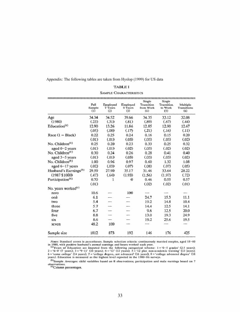
Table 1b and Table I (in the appendix) compare the women’s observable characteristics

between the sample used here and the sample used by Hyslop (1999) for U.S. data.2 In

Table 1b for Swedish data, women who always work are better educated (36% women have

1 The data used in the analysis are drawn from the Swedish Longitudinal Individual Data (LINDA). LINDA, a joint endeavor between the Department of Economics at Uppsala University, The National Social Insurance Board (RFV), Statistics Sweden (the main administrator), and the Ministries of Finance and Labor, is a register based data set consisting of a large panel of individuals, and their household members. The sampling procedure ensures that each annual cross section is representative for the population that year. The sample consists of 236,740 married couples, aged 20 to 60 in 1992-2001. 2 The data used by Hyslop (1999) are from the 1986 panel study of income dynamics (PSID) and pertain to the seven calendar years 1979-85, corresponding to waves 12-19 of the PSID and the sample consists of 1812 continuously married couples, aged between 18 and 60 in 1980. Sample characteristics are included in the Appendix (Hyslop Table I).

4

University education) than those who never work (9% women have University education).

In Table I for US data, women who always work are also better educated (average years of

education is 13.26) than those who never work (average years of education is 11.86).

Table-1b>>>

In Table 1b, women who always work have fewer dependent children and their husband’s

earnings are considerably higher than those who never work. On the other hand, in Table I,

women who always work have fewer dependent children but their husband’s earnings are

lower than those who never work.

Swedish women who experience a single transition from work are older and have fewer

infant children aged 0-2. However Swedish women who experience a single transition to

work or who experience multiple transitions are younger than average, and have

considerably more dependent children. Their husband’s earnings are slightly bellow

average. The U.S. women who experiences a single transition to work are younger than

average while their husband’s earnings is higher than average. The U.S. women who

experiences multiple transitions are also younger than average but their husband’s earnings

is lower than average. The differences in the total number of dependent children between

the first four columns and the last two for both countries (especially Sweden) correspond

with age differences. The presence of dependent children, together perhaps with lower than

average husband’s earnings, may increase the probability of frequent employment

5

transitions, especially in Sweden which has more widely available childcare than in the

U.S.

In order to see the effect of observable characteristics on participation decisions, we

analyzed the following variables:

Employment status: There are two different labor market states. An individual is defined as

a participant if they report both positive annual hours worked and annual earnings3.

Age: Married couples aged 20 to 60 in 1992 are included in the sample.

Education: Educational attainment is included since there may be different participation

behavior among different educational groups. Three dummy variables for educational

attainment are used: one for women who have at most finished Grundskola degree (9 years

education); one for women who have Gymnasium degree (more than 9 but less than 12

years of education); and one for women who have education beyond Gymnasium (high

school).

Fertility variables: Number of children aged 0-2, 3-5 and 6-7 are defined as fertility

variables.

Place of birth: In the sample it is observed that Swedish born women (93%, who work all

ten years) work more than the foreign born women (85%, who never work). A dummy

3 To avoid part-time earnings and earnings from short unemployment, the individuals with earnings lower than a threshold level are considered as non participant.

6

variable for place of birth is included to see if there is any difference in the participation pattern

between Swedish born and foreign born individuals. This dummy variable indicates the

immigration status of the individual, where 1 refers to native born and 0 otherwise.

Husband’s earning: Husband’s earning is used as a proxy for non-labor income. The time

average ( .iy ) of husband’s earnings is used as permanent income (ymp); while the

deviations from the time average ( .iy ) is transitory income (ymt). Annual earnings are

expressed in constant (2001) SEK4, computed as nominal earnings deflated by the

consumer price index.

Future birth: An indicator variable for whether a birth occurs next period is also included.

3 The Empirical model

The empirical model used here is, similar to that used by Hyslop (1999). The model is a

simple dynamic programming model of search behavior under uncertainty, in which search-

costs associated with labor market entry and labor market opportunities differ according to

the individual’s participation state.

41 US Dollar = 10.7962 Swedish Kroner (2000-06-01).

7

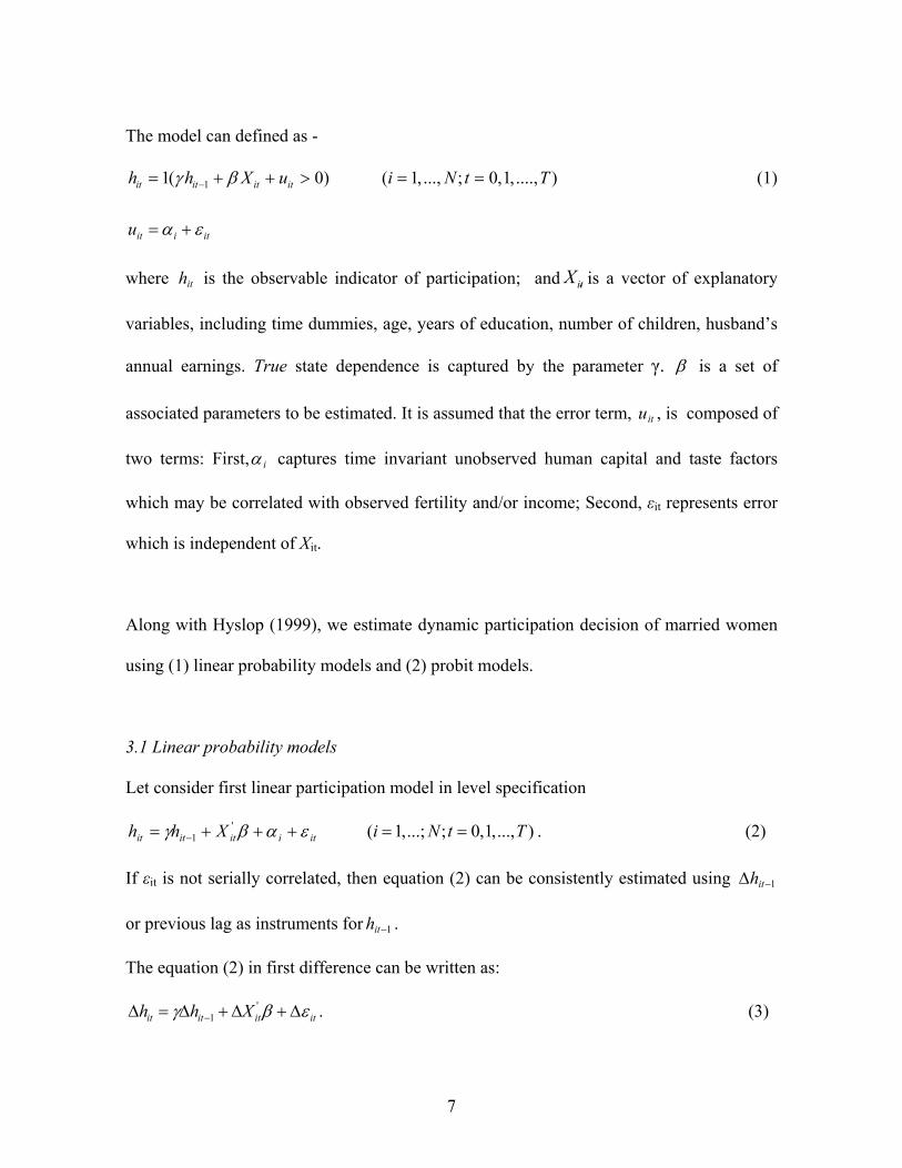
The model can defined as -

11( 0) ( 1, ..., ; 0,1,...., )it it it ith h X u i N t Tγ β−= + + > = = (1)

itiitu εα +=

where ith is the observable indicator of participation; and itX is a vector of explanatory

variables, including time dummies, age, years of education, number of children, husband’s

annual earnings. True state dependence is captured by the parameter γ. β is a set of

associated parameters to be estimated. It is assumed that the error term, itu , is composed of

two terms: First, iα captures time invariant unobserved human capital and taste factors

which may be correlated with observed fertility and/or income; Second, εit represents error

which is independent of Xit.

Along with Hyslop (1999), we estimate dynamic participation decision of married women

using (1) linear probability models and (2) probit models.

3.1 Linear probability models

Let consider first linear participation model in level specification

itiititit Xhh εαβγ +++= −'

1 ( 1,...; ; 0,1,..., )i N t T= = . (2)

If εit is not serially correlated, then equation (2) can be consistently estimated using 1−∆ ith

or previous lag as instruments for 1−ith .

The equation (2) in first difference can be written as:

'1it it it ith h Xγ β ε−∆ = ∆ + ∆ + ∆ . (3)

8

If εit is not serially correlated, then equation (3) can be consistently estimated using 2−ith or

previous lags and non-contemporaneous realizations of the covariates as instrument

for 1−∆ ith .

Even if itε is serially correlated, it can be consistently estimated by two-step procedure

using 2−ith as instrument for 1−∆ ith However if itε follows an AR(1) process:

ititit v+= −1ρεε , where -1< ρ <1, ),0(~ 2σitv , we can eliminate the serial correlation in the

errors as :

itiititititit vXXhhh +−+−+−+= −−− αρρββργγρ )1()( 1'

21 . (4)

Then equation (4) can be consistently estimated by instrumenting for 1−ith and 2−ith using

1−∆ ith and 2−∆ ith . Alternatively, first-difference of (4) gives the equation:

itititititit vXXhhh ∆+∆−∆+∆−∆+=∆ −−− ρββργγρ 1'

21)( . (5)

In this case, 2−ith is a valid instrument for 1−∆ ith 5.

3.2 Non-linear models

11( 0)it it it i ith h Xγ β α ε−= + + + > (6)

itiitu εα += and ),0(~ 2εσε Nit ( 1,...; ; 1,..., )i N t T= =

where ith is the indicator variable for participation and itX is a vector of explanatory

variables, including time dummies, age, years of education, number of children, husband’s

annual earnings. The subscript i indexes individuals and the subscripts t indexes time

5 For more details see, Hyslop (1999).

9

periods. The parameter γ represents true state dependence whereby an individual’s

propensity to participate is changed because of past participation. iα represents for all

unobserved determinants (such as taste for work, intelligence, ability, motivation or

general attitude of individuals) of participation that are time invariant for an individual i.

And finally itε represents the idiosyncratic error term.

The equation (6) can be estimated by random effect probit model using MLE. The standard

(uncorrelated) random effect model assumes that iα is uncorrelated with itX . But if the

number of children and/or income is correlated with unobserved tastes, as expected in this

paper, then iα will be correlated with itX . Hence we consider the correlated random effects

model (CRE) which is based on the following relationship between iα and the observed

characteristics6:

1 2 31

41

( (# 0 2) (# 3 5) (# 6 17) )T

i s is s is s iss

T

s mis is

Kids Kids Kids

y

α δ δ δ

δ η

=

=

= − + − + −

+ +

∑

∑

Thus the model (6) can be written as:

( )1 1`

1( 0)it it t it s is i its t

h h X Xγ β δ δ η ε−≠

= + + + + + >∑ (7)

it i itv η ε= + ( 1,...; ; 1,..., )i N t T= =

where ),0(~ 2ηση iidNit and independent of itX and i tε for all i, t.

6 There is substantial literature concerned with this issue. See for example Mundlak (1978), Chamberlain (1984).

10

The initial condition in dynamic probit model with unobserved effects complicates

estimation considerably. Estimation requires an assumption about the relationship between

the initial observations, 0ih , and iη .We consider the approach to the initial conditions

problem proposed by Heckman (1981b). The model specifies a linearized reduced form

equation for the initial period as:

( )´0 0 0 0 01 0i i ih zβ η ε= + + > (8)

where 20 0~ (0, )iidN ηη σ and independent of 0iz and 0iε . 0iz includes the variables for

initial period ( 0iX ) and other exogenous variables. It is also assumed that the error term

0iε satisfies the same distributional assumptions as itε for t ≥ 1. For normalization we

assume 2 1εσ = .

For a random sample of individuals the likelihood to be maximized is then given by

( ) ( ){ } ( ) ( ) ( )´0 0 0 0 1 1

`1 1

2 1 2 1N T

i i it t it s is i its ti t

L z h h X X h dFη

β η γ β δ δ η η−≠= =

⎧ ⎫⎡ ⎤⎛ ⎞⎪ ⎪⎡ ⎤= Φ + − Φ + + + + −⎨ ⎬⎢ ⎥⎜ ⎟⎣ ⎦ ⎝ ⎠⎪ ⎪⎣ ⎦⎩ ⎭∑∏ ∏∫ (9)

where F is the distribution function of η (consisting of 0η and iη ). However, as η is not

observed, we have to integrate out this term from the above likelihood to obtain the

unconditional likelihood function. To do this, we need to specify a distribution for η . If η

is taken to be normally distributed, the integral over η can be evaluated using Gaussian—

Hermite quadrature (Butler and Moffitt, 1982). In this paper, we follow an alternative

11

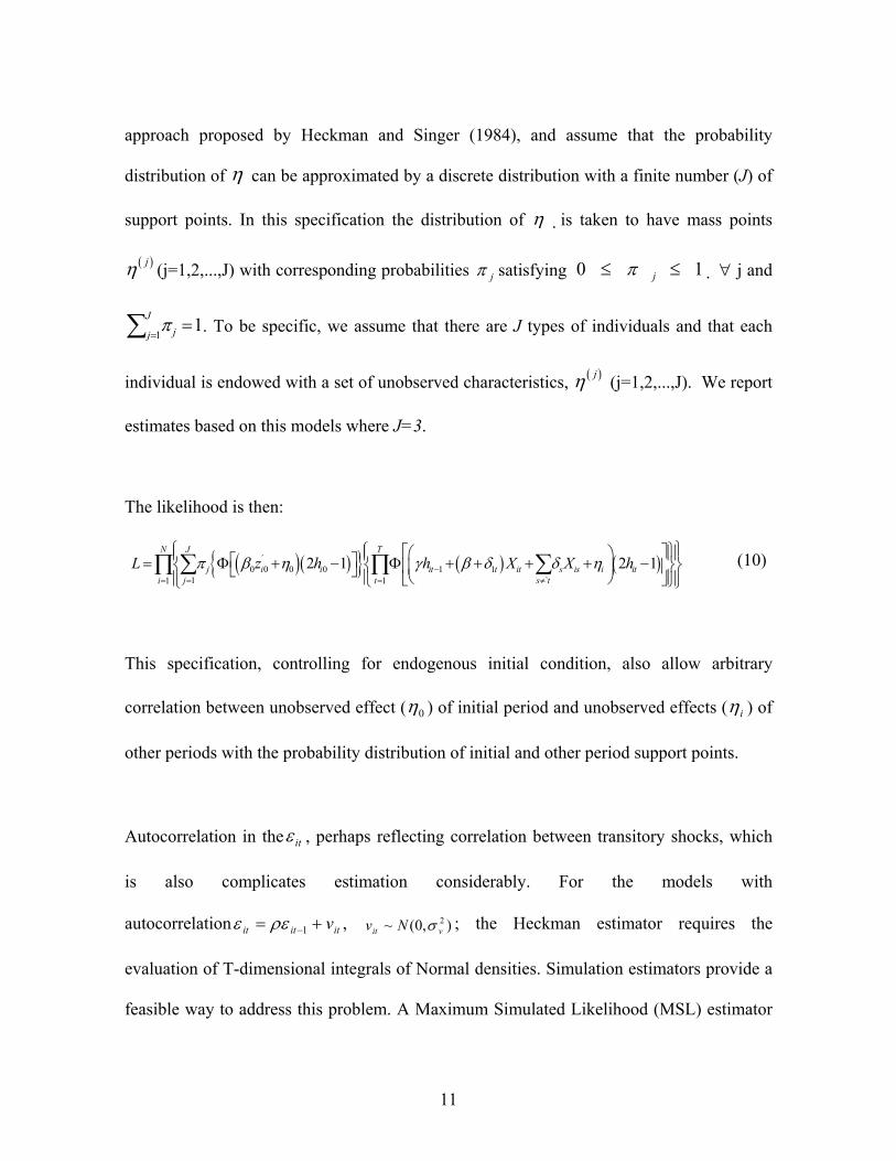
approach proposed by Heckman and Singer (1984), and assume that the probability

distribution of η can be approximated by a discrete distribution with a finite number (J) of

support points. In this specification the distribution of η is taken to have mass points

( )jη (j=1,2,...,J) with corresponding probabilities jπ satisfying 0 1jπ≤ ≤ ∀ j and

11J

jjπ

==∑ . To be specific, we assume that there are J types of individuals and that each

individual is endowed with a set of unobserved characteristics, ( )jη (j=1,2,...,J). We report

estimates based on this models where J=3.

The likelihood is then:

( )( ){ } ( ) ( )´0 0 0 0 1 1

1 `1 1

2 1 2 1N TJ

j i i it t it s is i itj s ti t

L z h h X X hπ β η γ β δ δ η−= ≠= =

⎧ ⎫⎧ ⎫⎡ ⎤⎛ ⎞⎪ ⎪ ⎪⎪⎡ ⎤= Φ + − Φ + + + + −⎨ ⎨ ⎬⎬⎢ ⎥⎜ ⎟⎣ ⎦ ⎝ ⎠⎪ ⎪⎣ ⎦⎪ ⎪⎩ ⎭⎩ ⎭∑ ∑∏ ∏ (10)

This specification, controlling for endogenous initial condition, also allow arbitrary

correlation between unobserved effect ( 0η ) of initial period and unobserved effects ( iη ) of

other periods with the probability distribution of initial and other period support points.

Autocorrelation in the itε , perhaps reflecting correlation between transitory shocks, which

is also complicates estimation considerably. For the models with

autocorrelation ititit v+= −1ρεε , ),0(~ 2vit Nv σ ; the Heckman estimator requires the

evaluation of T-dimensional integrals of Normal densities. Simulation estimators provide a

feasible way to address this problem. A Maximum Simulated Likelihood (MSL) estimator

12

(see for example Gourieroux and Monfort, 1996, and Cameron and Trivedi, 2005), based

on the GHK algorithm of Geweke, Hajivassiliou and Keane (see for example Keane, 1994)

can be used. The above model and estimator are discussed in Lee (1997) in more details.

Following Lee (1997) first we generate 1 2, ,..., Tu u u independent uniform [0, 1] random

variables. Then with given initial condition the truncated random variables 1 2, ,..., Tw w w

for GHK simulator can be generated recursively from the following steps, from t=1….,T:

(1) Calculate ( ) ( ) ( )11 1 1

`2 1 2 1t it t it it t it s is i it

s tw h u h h X Xγ β δ δ η ρε−

− −≠

⎡ ⎤⎛ ⎞⎛ ⎞= − − Φ Φ − + + + + +⎢ ⎥⎜ ⎟⎜ ⎟⎝ ⎠⎝ ⎠⎣ ⎦

∑ .

(2) Update the disturbances process 1t it itwε ρε −= +

For each i, with R independently generated vectors from random draws the simulated

likelihood is

( ) ( ){ } ( ) ( )´0 0 0 0 1 1 , 1

1 1 `1 1

1 2 1 2 1N TR J

rj i i it t it s is i i t it

r j s ti t

L w z h h X X hR

β η γ β δ δ η ρε− −= = ≠= =

⎡ ⎤⎧ ⎫⎧ ⎫⎡ ⎤⎛ ⎞⎪ ⎪ ⎪⎪⎡ ⎤= Φ + − Φ + + + + + −⎢ ⎥⎨ ⎨ ⎬⎬⎢ ⎥⎜ ⎟⎣ ⎦ ⎝ ⎠⎪ ⎪⎢ ⎥⎣ ⎦⎪ ⎪⎩ ⎭⎩ ⎭⎣ ⎦∑ ∑ ∑∏ ∏ (11)

13

4 Results

This section reports and compares the results with the results of Hyslop (1999) for various

linear probability models and probit models. The results for all specifications are reported

based on 10% (random draw) sub-sample. 7

4.1 Linear Probability Models

Various dynamic linear probability specifications corresponding to equation (2) and (3)

have been estimated both in levels and in first difference specification, just as Hyslop

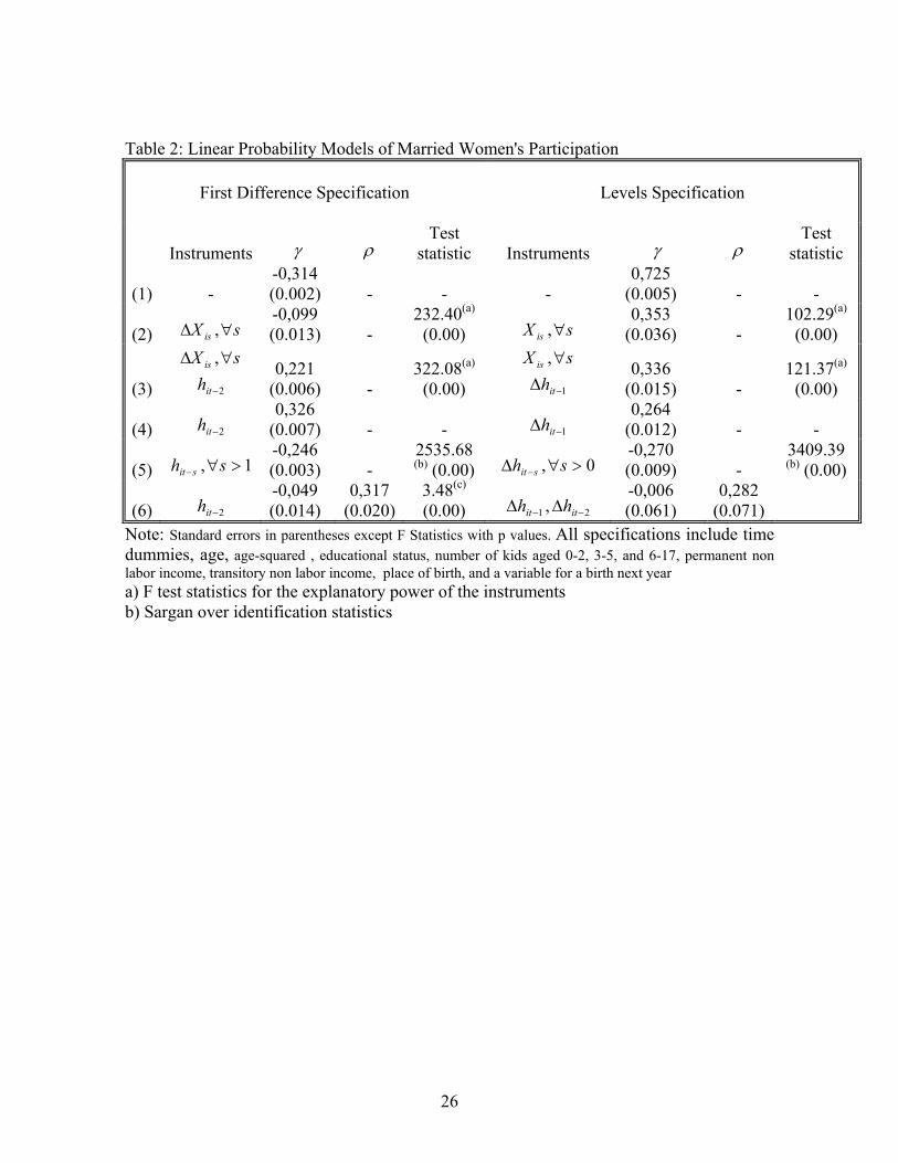
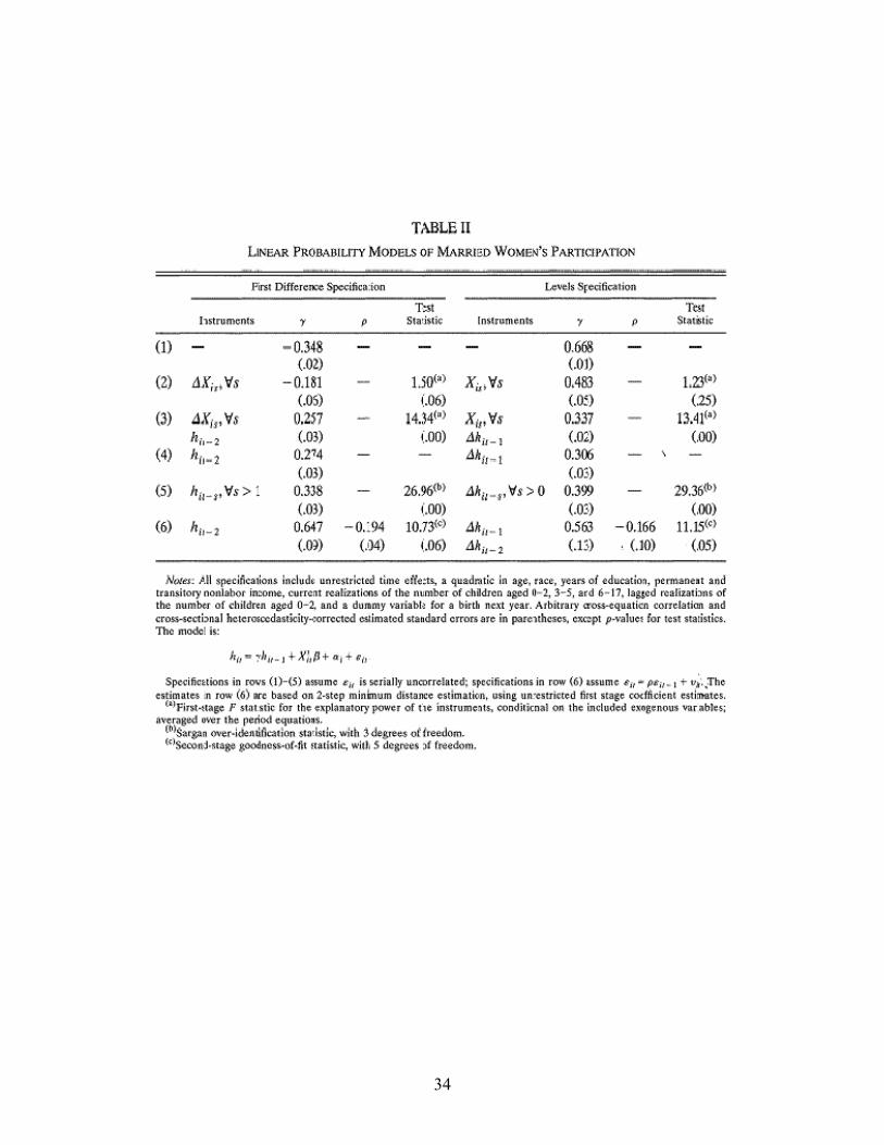
(1999) did. Table 2 shows the results for seven years data. In row 1, the GLS estimate of

lagged dependent variable for first difference is -0.31 which is downwards biased due to

negative correlation between 1−∆ ith and the error due to first differencing. While the

estimate obtained from level specification is 0.73 which is upwards biased because of

unobserved heterogeneity. These findings are very close to Hyslop’s GLS findings for

lagged dependent variables. The estimates for first difference and level specifications in

Hyslop (1999) are -0.35 and 0.67 respectively (See appendix row 1 Table II).

Row (2) shows the results using out-of-period realizations of the covariates as instruments

for the lagged dependent variable. If the regressors are exogenous with respect to the

transitory error component, these instruments are valid instruments and enable consistent

estimates of the effects of lagged dependent variable. Estimated coefficients in first

difference and level specification are: -0.10 and 0.35 respectively. These coefficients are

close to zero than the GLS estimates.

14

If it is assumed that there is no serial correlation in the transitory errors then lagged values

of h would be valid instruments for 1−∆ ith , and lagged values of h∆ would be valid

instruments for 1−ith . In row 3, 2−ith is added to the vector of instruments for 1−∆ ith , and

1−∆ ith to the vector of instruments for 1−ith . The estimates of the lagged dependent variable

coefficients obtained from the first difference and level specification are now 0.22 and 0.34

respectively. The F-statistics indicate that these instruments have substantial explanatory

power. In row 4, the regressors have been dropped form the instrument sets. The

coefficients of lagged dependent variable are 0.32 to 0.26. Row (5) shows the specifications

based on Arellano and Bond (1991), which include all valid lagged participation effects in

the instrument sets. The estimated coefficients for first-differences and levels are very

close, -0.24 and -0.27, respectively. Finally row (6) presents the specification which relaxes

the assumption that the transitory errors are uncorrelated, and allows the errors to follow a

stationary AR(1) process. Two-step GMM estimation shows that the coefficients of lagged

dependent variable in both first difference and level specification decreased dramatically to

-0.05 and -0.006 respectively. On the other hand, the estimates of the AR(1) serial

correlation parameter are positive and quite similar: 0,32and 0.28 respectively.

Interestingly, the results of GMM contrast sharply with Hyslop(1999). In Hyslop(1999), the

effects of lagged dependent variable are positive, while AR(1) coefficients are negative. We

will check these contrasts by another specification.

Table-2>>>

15

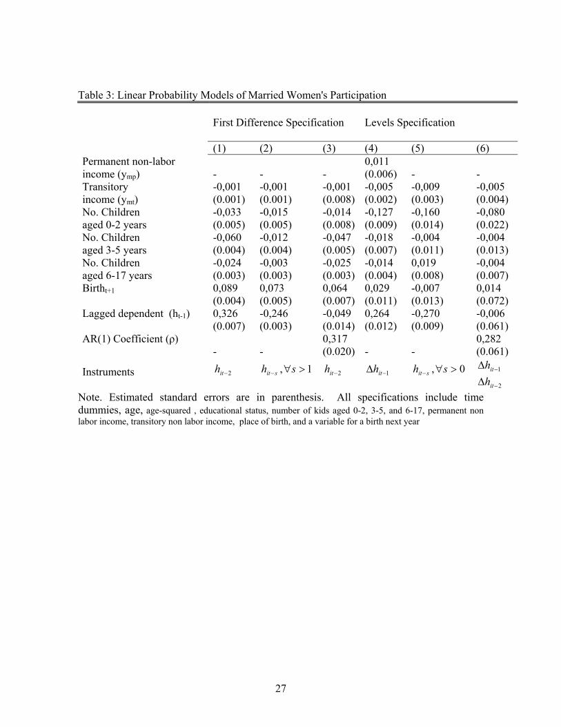
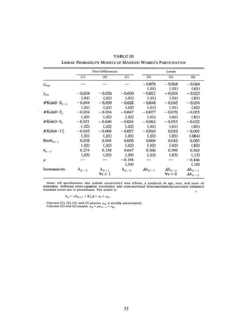
Table 3 shows the estimated regressor coefficients from the specifications presented in

rows (4)-(6) of Table 2. Like Hyslop’s findings (See appendix Table III), the results show

that pre-school children have substantially stronger effects on participation outcomes than

school-aged children. The results also show that permanent non-labor income effect (ymp) is

positive and significant.

Table-3>>>

4.2 Static probit models

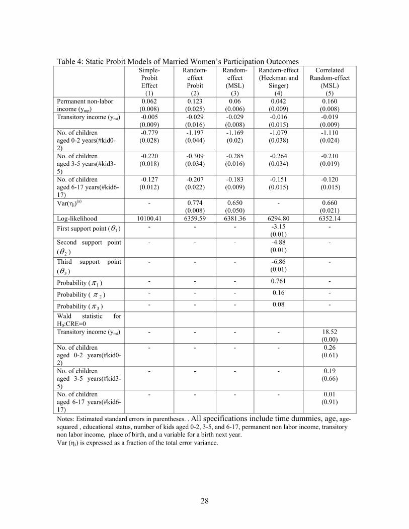
Table 4 shows the results for the static probit specifications focusing on demographic and

other characteristics of married women in Sweden. Here, the model is estimated for the

sample over the ten year period (1992-2001). Column 1 contains the results of simple

probit model where each of the fertility variables has significantly negative effect on

women’s participation decisions. The younger children have stronger effects than older. An

additional child aged 0-2 reduces the probability of participation by 18 percent (marginal

effect). The permanent non-labor income effect is significantly positive which may reflect

the predominant dual income family structure in Sweden.

Table -4>>>

Column 2 contains the results of random effects probit model estimated by MLE using

Gaussian quadrature. The result indicates that 77 percent of the latent error variance is due

to unobserved heterogeneity. Compared to simple probit model, the estimated effects of

16

young children aged 0-2 increase by 53 percent while that of children aged 6-17 increases

by 62 percent. The random effect probit model is re-estimated considering two different

types of distribution of unobserved heterogeneity. In column 3 the heterogeneity is assumed

to be normally distributed whereas in column 4 it is assumed that the heterogeneity have a

common discrete distribution with a finite number of mass points (Heckman and Singer

approach). The estimates of these models are broadly similar.

The estimated support points and accompanying probabilities for the model in column 4

indicate unobserved heterogeneity in individuals’ preferences. The first estimated support

point ( 1θ = -3.15) and the corresponding probability ( 1π = 0.761) indicate a relatively

strong preference for work by 76% of the sample (compared to the sample information that

58% actually work all 10 years of the study period). The second estimated-support point

( 2θ = -4.88) and the corresponding probability ( 2π = 0.156) indicates flexible preference

for work by 16%. The third estimated support point ( 3θ = -6.86) and the corresponding

probability ( 3π = 0.083) indicates low preference for work by 8% (compared to the sample

information that 5% don’t work at all during the study period).

It has been assumed that the fertility and/or income variables are independent of

unobserved heterogeneity. If these assumptions are incorrect, the resulting coefficient

estimates will be biased and inconsistent. For this reason the correlated random effects

(CRE) specification for iα , given in equation (7) is estimated in column 5. A likelihood

ratio test (not reported) of simple versus correlated random effects models gives no support

17

for rejecting the simple model (LR statistic = 14.97). Moreover, separate Wald–statistics

for the correlation between unobserved heterogeneity and three fertility variables provide

evidence in favor of exogeneity hypothesis in each case. These findings sharply contradict

Hyslop (1999) finding in static case, who rejects the hypothesis that fertility decisions are

exogenous to women’s participation decisions.

4.3 Dynamic probit models

Table 5 shows the results of inter-temporal participation decisions of married women. A

latent class ( model is used in the dynamic probit model with unobserved individual

specific effect. Column 1 contain the results for the specification which allows first order

autoregressive error AR(1).The results show that the addition of a transitory component of

error has significant effect on the model and the estimated coefficient is 0.81. The

percentage of the women of strong preference for work is now increased to 13%.

Column 2 contains the results for the specification which allows first order state

dependence SD(1). This specification allows arbitrary correlation between the initial and

other periods with the same probability of initial and other periods support points. The

results show a large first order state dependence effect and the coefficient is 1.28.

Column 3 shows the results for the random effects specifications with a first order

autoregressive error component AR(1) and first order state dependence SD(1). The model

is estimated using simulated maximum likelihood (MSL) estimation method and based on

18

two support points.7 For simulation I use standard approach to random draws from the

specified distribution. The results show that including state dependence has a little effect on

the distribution of unobserved heterogeneity and serial correlation parameter in the model.

The AR(1) coefficient is now 0.86.

4.4 Simulated responses to “fertility” and to changes in “non-labor” Income

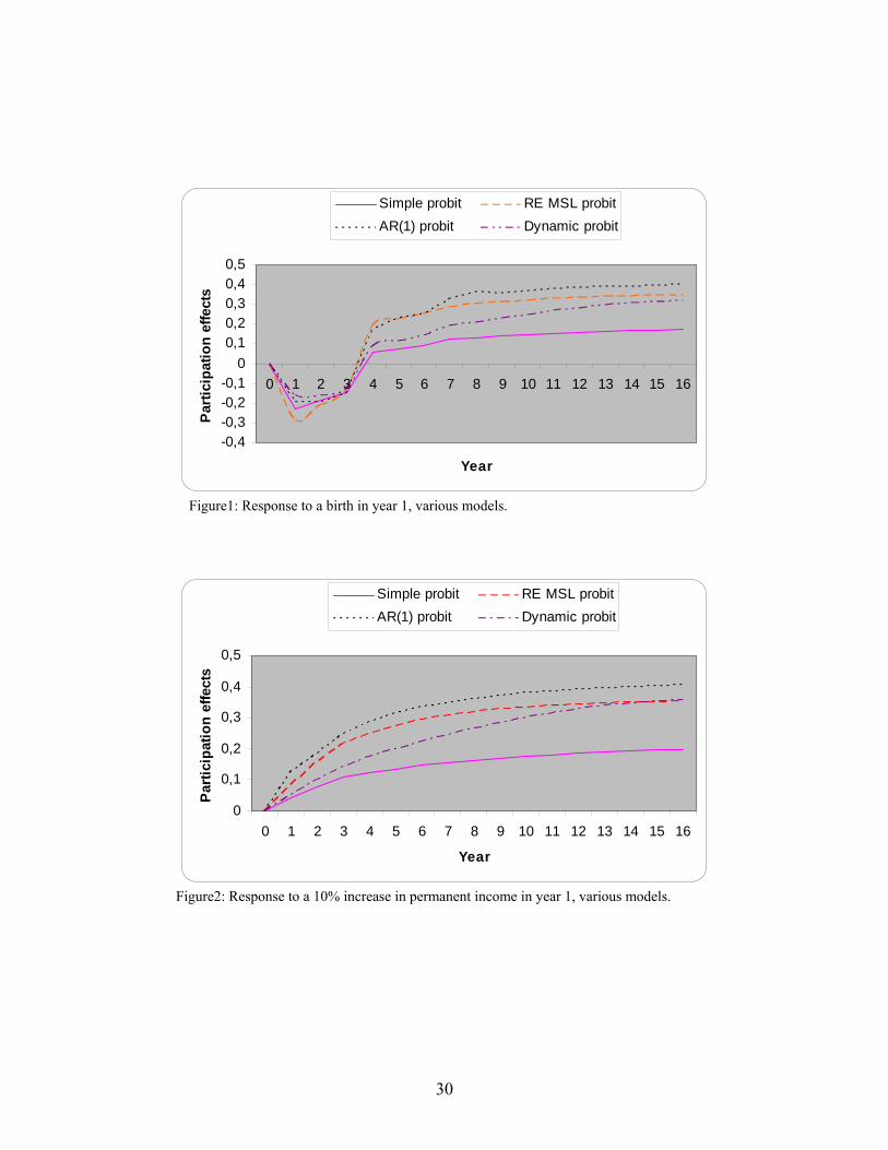
Figure 1 shows simulated responses to a birth in year 1 for the simple probit model, random

effects MSL probit model, AR(1) probit model, and dynamic probit with first order state

dependence model. The effect of an additional child aged 0-2 is -0.18 in simple probit, -

0.21 in RE MSL, -0.19 in AR (1), and -0.16 in dynamic probit. The difference between

simple probit and RE-MSL shows the bias due to unobserved heterogeneity. However, the

distance between RE-MSL and dynamic probit shows the bias that arises from not

controlling for state dependence. The simulated responses decline initially as the child ages,

and are nearly indistinguishable when the age is 3. The simulation patterns explain that the

women leave the labor force to have children and return as the children age beyond infancy.

The return of Swedish women to work is quicker than the US women (See Hyslop 1999).

This indicates that Sweden has more widely available childcare system than the U.S.

7 The model is also estimated with three support points and found that the model is fitted well with two support points (for this and other results concerning this issue, see Hansen and Lofstrom 2001, Cameron and Heckman 2001, Stevens 1999, Ham and Lalonde 1996, Eberwein, Ham and Lalonde 1997). This issue is also discussed in Heckman and Singer.

19

Figure 2 shows the simulated effects of ten percent increase in permanent non-labor

income. Ten percent increase in permanent non-labor income increases women’s

participation in the first year by 0.08 in simple-probit, 0.16 in RE-MSL, and 0.10 in

dynamic probit. The figure suggests that there is a positive income effect of husbands’

earnings on wives’ participation decision.

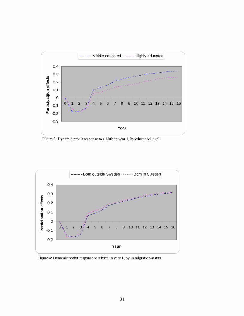
Figure 3 shows the dynamic probit model responses to a birth during first year for middle

educated (Gymnasium) and highly educated (University) women. The results show that the

effect of one birth during first year for middle educated women is stronger than those of

highly educated. Figure 4 shows broadly similar responses of immigrant and native born

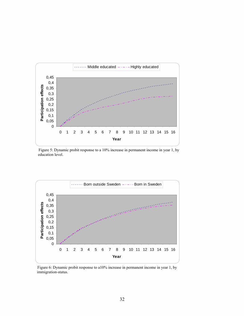
women. Figure 5 presents the dynamic probit model responses of 10 percent increase in

permanent non-labor income for middle educated (Gymnasium) and highly educated

(University) women. The response of dynamic probit model for middle educated women is

stronger than those of highly educated. Figure 6 shows quite similar responses of

immigrant and native born women.

5 Summary and Conclusions

The purpose of this study is to analyze the inter-temporal labor force participation

behavior of married women in Sweden, using a ten year sample from Longitudinal

Individual Data (LINDA). We estimated linear probability models and dynamic probit

models with a variety of specifications. Both linear probability and probit results suggest

that the inter-temporal participation decisions are characterized by a substantial amount of

20

unobserved heterogeneity. In the specification which allows first order state dependence

and serial correlation in the transitory errors components, it is found that almost no true

state dependence in individual propensities to women participation. However the estimated

first order AR(1) component has a large and significant effect in both linear probability

model and dynamic probit model. The findings indicate serial persistence on participation

decisions due to persistent individual heterogeneity

21

References

Arellano, M., and S. Bond (1991), “Some Tests of the Specification for Panel Data: Monte

Carlo Evidence and an Application to Employment Equations”, Review of Economic

Studies, 58,277-297.

Butler, J.S., and R. Moffitt (1982), “A Computationally Efficient Quadrature Procedure for

the One Factor Multinomial Probit Model”, Econometrica, 50, 761-764.

Cameron, S., and J.J. Heckman (2001), “The Dynamics of Educational Attainment for

Black, Hispanic, and White Males,” Journal of Political Economy 109(3):455-499.

Cameron A. Colin and Pravin K. Trivedi (2005) Microeconometrics : Methods and

Applications, Cambridge University Press.

Card, D., and D. Sullivan (1988), “Measuring the Effect of Subsidized Training Programs

on Movements In and Out of Employment”, Econometrica, 56, 497-530.

Chamberlain G. (1984) “Panel Data”, in Handbook of Econometrics, ed. By Z. Griliches

and M. Intrilligator, Amsterdam: North –Holland.

Eberwein, C., J. Ham, and R. Lalonde (1997), “The Impact of Being Offered and Receiving

Classroom Training on the Employment Histories of Disadvantaged Women: Evidence

from Experimental Data,” Review of Economic Studies 64(4):655-682.

22

Gourieroux, C. and A. Monfort (1996) Simulation-Based Econometric Method, Oxford

University Press.

Ham, J., and R. Lalonde (1996), “The Effect of Sample Selection and Initial Conditions in

Duration Models: Evidence from Experimental Data on Training,” Econometrica

64(1):175-205.

Hansen, J., and M. Lofstrom (2001), “The Dynamics of Immigrant Welfare and Labor

Market Behavior,” IZA Discussion Paper, No. 360, Institute for Study of Labor, Bonn.

Heckman, J. J. (1981a), “Statistical Models for Discrete Panel Data”, Chapter 3 in Manski, Charles

and Daniel McFadden (eds.), Structural Analysis of Discrete Data, MIT Press, Cambridge, MA.

Heckman, J. J. (1981b), “The Incidental Parameters Problem and the Problem of Initial Conditions

in Estimating a Discrete Time-Discrete Data Stochastic Process”, Chapter 4 in Manski, Charles and

Daniel McFadden (eds.), Structural Analysis of Discrete Data, MIT Press, Cambridge, MA.

Heckman, J. J. (1981c), “Heterogeneity and State Dependence”, in Rosen, Sherwin (ed.) Studies in

Labor Markets, University of Chicago Press.

Heckman, J.,J. and B. L. Singer (1984), “A Method for Minimizing the Distributional

Assumptions in Econometric Models for Duration Data”, Econometrica, 52, 271-320.

23

Hyslop, D. R. (1999), “State dependence, serial correlation and heterogeneity in inter

temporal labor force participation of married women”, Econometrica, 67, 1255-1294.

Keane, M. P. (1993), “Simulation Estimation for Panel Data Models with Limited

Dependent Variables”, Ch. 20 in Handbook of Statistics, Vol. 11, G.S. Maddala, C.R. Rao,

and H.D. Vinod (eds.). Amsterdam: Elsevier Science Publishers.

Keane, M. P. (1994), “A computationally Practical Simulation Estimator for Panel Data”,

Econometrica, 62, 95-116.

Lee, L.F. (1997), “Simulated Maximum Likelihood Estimation of Dynamic Discrete

Choice Statistical Models Some Monte Carlo Results”, Journal of Econometrics, 82, 1-35.

Lerman, S. R., and C. F. Manski (1981), “On the Use of Simulated Frequencies to

Approximate Choice Probabilities”, Ch. 7 in Structural Analysis of Discrete Data, Charles

Manski and Daniel Mc Fadden (eds.). Cambridge, MA, MIT Press.

McFadden, D. (1989), “A Method of Simulated Moments for Estimation of Discrete

Response Models without Numerical Integration”, Econometrica, 57, 995-1026.

Mundlak Y. (1978) “On the Pooling of Time Series and Cross Section Data”,

Econometrica, 46, pp.69-85.

24

Pakes, A. and D. Pollard (1989), “Simulation and Asymptotic of Optimization Estimators”,

Econometrica, 57, 1027-1057.

Phelps, E. (1972), “Inflation Policy and Unemployment Theory”, New York: Norton.

Stevens, A. (1999) “Climbing Out of Poverty, Falling Back In,” Journal of Human

Resources 34(3):557-588.

25

Table 1a: Distribution of Number of Years Worked Number of

years worked Full sample

(1)

Employed all 10 years

(2)

Employed 0 years

(3)

Single transition from work

(4)

Single transition to work

(5)

Multiple transitions

(6)

Zero 4.67 - 100 - - - One 1.49 - - 10.48 4.17 2.42 Two 1.56 - - 7.06 4.80 3.37 Three 1.74 - - 6.68 5.53 3.92 Four 2.16 - - 6.53 5.63 5.87 Five 2.41 - - 7.06 4.56 7.27 Six 3.46 - - 8.73 7.47 10.43 Seven 4.36 - - 10.86 10.62 12.68 Eight 6.97 - - 15.03 16.83 20.93 Nine 12.45 - - 27.56 40.40 33.13 Ten 58.73 100 - - - - Column percentages. Table 1b: Sample Characteristics

Full sample

(1)

Employed all 10 years

(2)

Employed 0 years

(3)

Single transition from work

(4)

Single transition to work

(5)

Multiple transitions

(6)

Age(1992) 42.92 (8.15)

45.03 (7.12)

45.73 (7.84)

46.04 (8.02)

37.98 (7.25)

37.94 (8.05)

Education( a) (Primary)

0.18 (0.38)

0.16 (0.37)

0.44 (0.50)

0.29 (0.45)

0.16 (0.37)

0.16 (0.36)

Education( a) (High-school)

0.50 (0.50)

0.48 (0.50)

0.47 (0.50)

0.51 (0.50)

0.54 (0.50)

0.56 (0.50)

Education( a) (Universitet)

0.32 (0.47)

0.36 (0.48)

0.09 (0.28)

0.20 (0.40)

0.29 (0.46)

0.29 (0.45)

Place of birth (Born in Sweden=1)

0.92 (0.27)

0.93 (0.26)

0.85 (0.36)

0.89 (0.31)

0.91 (0.29)

0.91 (0.29)

No. of children aged 0-2 years

0.13 (0.37)

0.05 (0.23)

0.09 (0.32)

0.06 (0.28)

0.25 (0.50)

0.31 (0.53)


0.20 (0.45)

0.10 (0.33)

0.14 (0.39)

0.10 (0.34)

0.40 (0.59)

0.40 (0.58)


0.95 (1.01)

0.89 (0.96)

0.82 (1.04)

0.67 (0.90)

1.38 (1.11)

1.04 (1.05)

Husband’s Earnings (SEK 100,000)

2.67 (1.73)

2.78 (1.78)

2.23 (1.63)

2.64 (1.90)

2.54 (1.51)

2.52 (1.60)

Participation 0.84 (0.37)

1.00 0.00 0.60 (0.49)

0.69 (0.46)

0.70 (0.46)

Sample size 236,740 139,030 11,070 13,170 20,620 52,850 Note: Standard errors in parentheses. Sample selection criteria: continuously married couples, aged 20-60 in 1992 with positive husband’s annual earnings and hours worked each year. (a) Three dummy variables for educational attainment are used: One for women who have at most finished Grundskola degree (9 years education); One for women who have Gymnasium degree (more than 9 but less than 12 years of education); and one for women who have education beyond Gymnasium (high school).

26

Table 2: Linear Probability Models of Married Women's Participation

First Difference Specification

Levels Specification

Instruments γ ρ Test

statistic Instruments γ ρ Test

statistic

(1) - -0,314 (0.002) - - -

0,725 (0.005) - -

(2) isX∆ , s∀ -0,099 (0.013) -

232.40(a) (0.00) isX , s∀

0,353 (0.036) -

102.29(a) (0.00)

(3) isX∆ , s∀

2−ith 0,221

(0.006) - 322.08(a)

(0.00) isX , s∀

1−∆ ith 0,336

(0.015) - 121.37(a)

(0.00)

(4) 2−ith 0,326

(0.007) - - 1−∆ ith 0,264

(0.012) - -

(5) sith − , 1>∀s -0,246 (0.003) -

2535.68 (b) (0.00) sith −∆ , 0>∀s

-0,270 (0.009) -

3409.39 (b) (0.00)

(6) 2−ith -0,049 (0.014)

0,317 (0.020)

3.48(c)

(0.00) 1−∆ ith , 2−∆ ith -0,006 (0.061)

0,282 (0.071)

Note: Standard errors in parentheses except F Statistics with p values. All specifications include time dummies, age, age-squared , educational status, number of kids aged 0-2, 3-5, and 6-17, permanent non labor income, transitory non labor income, place of birth, and a variable for a birth next year a) F test statistics for the explanatory power of the instruments b) Sargan over identification statistics

27

Table 3: Linear Probability Models of Married Women's Participation

First Difference Specification

Levels Specification

(1) (2) (3) (4) (5) (6) Permanent non-labor income (ymp) - - -

0,011 (0.006) - -

Transitory income (ymt)

-0,001 (0.001)

-0,001 (0.001)

-0,001 (0.008)

-0,005 (0.002)

-0,009 (0.003)

-0,005 (0.004)

No. Children aged 0-2 years

-0,033 (0.005)

-0,015 (0.005)

-0,014 (0.008)

-0,127 (0.009)

-0,160 (0.014)

-0,080 (0.022)


-0,060 (0.004)

-0,012 (0.004)

-0,047 (0.005)

-0,018 (0.007)

-0,004 (0.011)

-0,004 (0.013)


-0,024 (0.003)

-0,003 (0.003)

-0,025 (0.003)

-0,014 (0.004)

0,019 (0.008)

-0,004 (0.007)

Birtht+1

0,089 (0.004)

0,073 (0.005)

0,064 (0.007)

0,029 (0.011)

-0,007 (0.013)

0,014 (0.072)

Lagged dependent (ht-1)

0,326 (0.007)

-0,246 (0.003)

-0,049 (0.014)

0,264 (0.012)

-0,270 (0.009)

-0,006 (0.061)

AR(1) Coefficient (ρ) - -

0,317 (0.020) - -

0,282 (0.061)

Instruments

2−ith

sith − , 1>∀s

2−ith

1−∆ ith

sith − , 0>∀s

1−∆ ith

2−∆ ith Note. Estimated standard errors are in parenthesis. All specifications include time dummies, age, age-squared , educational status, number of kids aged 0-2, 3-5, and 6-17, permanent non labor income, transitory non labor income, place of birth, and a variable for a birth next year

28

Table 4: Static Probit Models of Married Women’s Participation Outcomes Simple-

Probit Effect

(1)

Random-effect Probit

(2)

Random-effect (MSL)

(3)

Random-effect (Heckman and

Singer) (4)

Correlated Random-effect

(MSL) (5)

Permanent non-labor income (ymp)

0.062 (0.008)

0.123 (0.025)

0.06 (0.006)

0.042 (0.009)

0.160 (0.008)

Transitory income (ymt) -0.005 (0.009)

-0.029 (0.016)

-0.029 (0.008)

-0.016 (0.015)

-0.019 (0.009)

No. of children aged 0-2 years(#kid0-2)

-0.779 (0.028)

-1.197 (0.044)

-1.169 (0.02)

-1.079 (0.038)

-1.110 (0.024)


-0.220 (0.018)

-0.309 (0.034)

-0.285 (0.016)

-0.264 (0.034)

-0.210 (0.019)


-0.127 (0.012)

-0.207 (0.022)

-0.183 (0.009)

-0.151 (0.015)

-0.120 (0.015)

Var(ηi)(a) - 0.774 (0.008)

0.650 (0.050)

- 0.660 (0.021)

Log-likelihood 10100.41 6359.59 6381.36 6294.80 6352.14 First support point ( 1θ ) - - - -3.15

(0.01) -

Second support point ( 2θ )

- - - -4.88 (0.01)

-

Third support point ( 3θ )

- - - -6.86 (0.01)

-

Probability ( 1π ) - - - 0.761 -

Probability ( 2π ) - - - 0.16 -

Probability ( 3π ) - - - 0.08 -

Wald statistic for H0:CRE=0

Transitory income (ymt) - - - - 18.52 (0.00)


- - - - 0.26 (0.61)


- - - - 0.19 (0.66)


- - - - 0.01 (0.91)

Notes: Estimated standard errors in parentheses. . All specifications include time dummies, age, age-squared , educational status, number of kids aged 0-2, 3-5, and 6-17, permanent non labor income, transitory non labor income, place of birth, and a variable for a birth next year. Var (ηi) is expressed as a fraction of the total error variance.

29

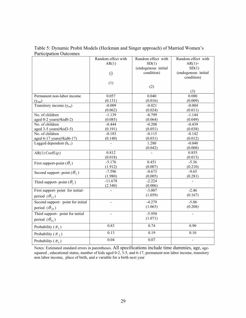
Table 5: Dynamic Probit Models (Heckman and Singer approach) of Married Women’s Participation Outcomes Random effect with

AR(1)

()

(1)

Random effect with SD(1)

(endogenous initial condition)

(2)

Random effect with AR(1)+ SD(1)

(endogenous initial condition)

(3) Permanent non-labor income (ymp)

0.057 (0.131)

0.040 (0.016)

0.080 (0.009)

Transitory income (ymt) -0.009 (0.062)

-0.021 (0.024)

-0.004 (0.011)


-1.139 (0.085)

-0.799 (0.064)

-1.144 (0.049)


-0.444 (0.191)

-0.208 (0.051)

-0.439 (0.038)


-0.183 (0.140)

-0.115 (0.031)

-0.142 (0.012)

Lagged dependent (ht-1) - 1.280 (0.042)

-0.040 (0.008)

AR(1) Coeff.(ρ) 0.812 (0.018)

- 0.855 (0.013)

First support-point ( 1θ ) -5.176 (1.912)

0.451 (0.007)

-5.36 (0.210)

Second support- point ( 2θ ) -7.596 (1.980)

-0.673 (0.005)

-9.65 (0.281)

Third support- point ( 3θ ) -11.678 (2.340)

-2.224 (0.006)

-

First support- point for initial- period ( 11θ )

- -3.007 (1.059)

-2.46 (0.167)

Second support- point for initial period ( 22θ )

- -4.279 (1.063)

-5.06 (0.208)

Third support- point for initial period ( 33θ )

- -5.950 (1.071)

-

Probability ( 1π ) 0.83 0.74 0.90

Probability ( 2π ) 0.13 0.19 0.10

Probability ( 3π ) 0.04 0.07 -

Notes: Estimated standard errors in parentheses. All specifications include time dummies, age, age-squared , educational status, number of kids aged 0-2, 3-5, and 6-17, permanent non labor income, transitory non labor income, place of birth, and a variable for a birth next year

30

-0,4-0,3-0,2-0,1

00,10,20,30,40,5

0 1 2 3 4 5 6 7 8 9 10 11 12 13 14 15 16

Year

Parti

cipa

tion

effe

cts

Simple probit RE MSL probitAR(1) probit Dynamic probit

Figure1: Response to a birth in year 1, various models.

0

0,1

0,2

0,3

0,4

0,5

0 1 2 3 4 5 6 7 8 9 10 11 12 13 14 15 16

Year

Parti

cipa

tion

effe

cts

Simple probit RE MSL probitAR(1) probit Dynamic probit

Figure2: Response to a 10% increase in permanent income in year 1, various models.

31

-0,3

-0,2

-0,1

0

0,1

0,2

0,3

0,4

0 1 2 3 4 5 6 7 8 9 10 11 12 13 14 15 16

Year

Parti

cipa

tjion

effe

cts

Middle educated Highly educated

Figure 3: Dynamic probit response to a birth in year 1, by education level.

-0,2

-0,1

0

0,1

0,2

0,3

0,4

0 1 2 3 4 5 6 7 8 9 10 11 12 13 14 15 16

Year

Parti

cipa

tion

effe

cts

Born outside Sweden Born in Sweden

Figure 4: Dynamic probit response to a birth in year 1, by immigration-status.

32

00,050,1

0,150,2

0,250,3

0,350,4

0,45

0 1 2 3 4 5 6 7 8 9 10 11 12 13 14 15 16

Year

Parti

cipa

tion

effe

cts

Middle educated Highly educated

Figure 5: Dynamic probit response to a 10% increase in permanent income in year 1, by education level.

00,050,1

0,150,2

0,250,3

0,350,4

0,45

0 1 2 3 4 5 6 7 8 9 10 11 12 13 14 15 16

Year

Parti

cipa

tion

effe

cts

Born outside Sweden Born in Sweden

Figure 6: Dynamic probit response to a10% increase in permanent income in year 1, by immigration-status.

33

Appendix: The following tables are taken from Hyslop (1999) for US data

34

35

Dynamic labour force participation of married women in Sweden

Documents