• • •

Welcome message from author
This document is posted to help you gain knowledge. Please leave a comment to let me know what you think about it! Share it to your friends and learn new things together.
Transcript

Durham E-Theses
Yang-Mills theories in curved space-times
Dolan, Brian P.
How to cite:
Dolan, Brian P. (1981) Yang-Mills theories in curved space-times, Durham theses, Durham University.Available at Durham E-Theses Online: http://etheses.dur.ac.uk/7398/
Use policy
The full-text may be used and/or reproduced, and given to third parties in any format or medium, without prior permission orcharge, for personal research or study, educational, or not-for-pro�t purposes provided that:
• a full bibliographic reference is made to the original source
• a link is made to the metadata record in Durham E-Theses
• the full-text is not changed in any way
The full-text must not be sold in any format or medium without the formal permission of the copyright holders.
Please consult the full Durham E-Theses policy for further details.
Academic Support O�ce, Durham University, University O�ce, Old Elvet, Durham DH1 3HPe-mail: [email protected] Tel: +44 0191 334 6107
http://etheses.dur.ac.uk
YANG-MILLS THEORIES IN CURVED SPACE-TIMES
by
Brian P. Dolan
A thesis presented for the degree of Doctor of Philosophy at the University of Durham
Mathematics Department University of Durham
July 1981
The copyright of this thesis rests with the author.
No quotation from it should be published without
his prior written consent and information derived
from it should be acknowledged.
"If you want to learn about nature, to appreciate nature,
it is necessary to understand the language that she speaks
in."
R.P.Feynman, The Character of Physical Law (1964 Messenger Lectures)

CONT:ENTS
Abstract
Declaration
Acknowledgements
Chapter One
Introduction
Chapter Two
Projective Space Models in Two and Four Dimensions
Page
(i)
(ii)
(iii)
1
5
Chapter Three 25
Multi-Instanton Solutions of !iP1 in Curved Space-Times
Chapter Four 42
Self-Dual SU(2) Fields in Curved Space-Times
Chapter Five 61
SU(2) and U(l) Fields in
Chapter Six 75
U(l) Instantons in s2x s2
Chapter Seven 81
Conclusions
Appendix A - Quaternions
Appendix B - :Evaluation of Two Integrals
References
(i)
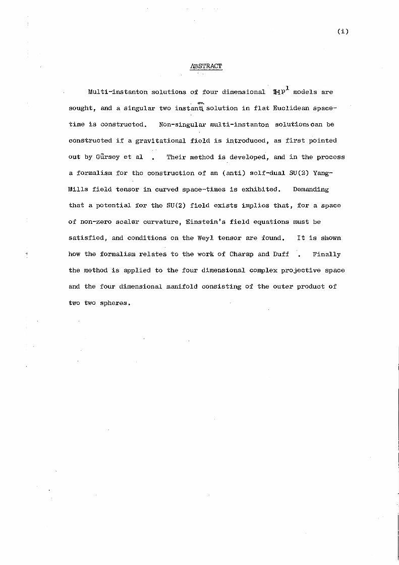
ABSTRACT
Multi-instanton solutions of four dimensional 1 lHP models are . 0'<\.
sought, and a singular two instan~solution in flat Euclidean space-
time is constructed. Non-singular multi-instanton s0lution~can be
constructed if a gravitational field is introduced, as first pointed
out by Gursey et al Their method is developed, and in the process
a formalism for the construction of an (anti) self-dual SU(2) Yang-
Mills field tensor in curved space-times is exhibited. Demanding
that a potential for the SU(2) field exists implies that, for a space
of non-zero scalar curvature, Einstein's field equations must be
satisfied, and conditions on the Weyl tensor are found. It is shown
how the formalism relates to the work of Charap and Duff Finally
the method is applied to the four dimensional complex projective space
and the four dimensional manifold consisting of the outer product of
two two spheres.

DECLARATION
YANG-MILLS THEORIES IN CURVED SPACE-TIMES
Ph.D. Thesis by Brian Patrick Dolan
The work for this thesis was carried out at the Department of
Mathematics, University of Durham, Durham, U.K., between October
197~ and July 1981. This thesis has not been submitted for any
other degree.
The latter part of chapter two was done in collaboration with
(ii)
Dr. D.B.Fairlie and Dr.W.J.Zakrzewski, and is claimed as original.
Chapters three, four, five and six are also claimed as original,
except where otherwise indicated. The first part of chapter three
is published in Journal of Physics A231and most of chapters four and
five is available as a Durham University pre-prinJ2~ Where other
authors have done similar work, they have been acknowledged in the
text.

(iii)
ACKNOWLEDGEMENTS
I wish to thank Ed Corrigan, William Deans, Lyndon Woodward,
Wojtek Zakrzewski and, in particular, my supervisor, David Fairlie,
who have taught me much about mathematics and physics and have been
invaluable sources of encouragement and advice. I also thank the
U.K. Science Research Council for studentship No. 78304719 under
which this research was carried out.

1.
CHAPTER 1
INTRODUCTION
-uv. At least three ofLfour forces of nature presently known,
electromagnetism and the strong and weak nuclear forces, seem to be
described by gauge theories, of the type first enunciated by Yang
Gauge theories of the fourth force, gravity
h 1 b d 1 d Ut . (60) K"bbl~7] I t· 1 th ave a so een eve ope , ~yama , ~ . .e • n par ~cu ar e
symmetry of the strong nuclear force is widely believed to be SU ( :3) -
chromodynamics. The evidence for SU(3) of colour is manifold,
though indirect17l The most compelling evidence is,
(i) The ratio)R,of the amplitudes for e+e- ~(hadrons) over
e+·e- ~ (leptons), depends on the numberof quarks and their charges.
For energies below charmed threshold, with only three flavours of
quark, i = 1,2,3 with charges ei,
::::= S 2/3 1 no colour
l 2, three colours.
Experiment favours the coloured case.
(ii) 0
The rate for the 1r to decay into two photons, again
depends on the number of quarks in the pion, their charges and the
(1)
direction of their isopins in isopin space. The amplitude is proportional
to
= t 1/6, no colour
l/2,three colours
Experiment favours the coloured case.
(iii) With only one type of quark for each flavour, the Pauli
(2)
exclusion principle forbids three quarks of the same flavour to be in
the same state. However, if each
2.
quark can come in three different colour states, they can all have the
same spin without violating the e~usion principle.
Thus, in any attempt to understand the colour force, it is very important
to analyse the Yang-Mills equations for a no:ti-abeHan SU(3) gauge theory.
Unfortunately, explicit solutions are difficult to find, though
At . ah t 1(4] h . d f . t t. 11 J.y e a ave gJ.ven a proce ure or -implicitly cons rue J.ng a
solutions for which the field tensor is (anti) self-dual • These
solutions are topologically non-trivial, a fact which owes its existence
to the four dimensional nature of the world in which we live. Since
the topological charge density can be written as a total divergence,
itdependsonly on the value of the gauge fields at very large distances
from the origin, i.e. on the "surface at infinity", s3 • The topological
3 charge is the winding number of the map from S to the gauge group1given
by the fields at infinity. It is a remarkable fact, that for any
simple lie group G
Thus the maps fall into topologically inequivalent classes, labelled
by the integers, ?__. [l]•
In order to try and understand SU(3) better, it is useful to
examine the case of SU(2). [6 44)
Here, explicit solutions are known ', ·
the 'tHooft solutions. These solutions are localised in both
E~-clidean space and time, and so are called "instantons". Since
instantons have non-zero action, they will contribute to the quantum
mechanical functional integral for the Yang-Mills fields and it has
been suggested that they may provide a mechanism for the confinement
of quarkJ14~ Indeed, for a simplified, two dimensional U(l) gauge
(3)
1 theory, <CP , the functional integral can be explicitly evaluated and
a logarithmic, confining potential between "instanton quarks" has been

3.
tl9 20] demonstrated ' • To try and extend this to SU(2) in four dimensions,
it is a very compelling step to consider quaternionic fields, and this
h h b . f ·· th t'30 1 381 451 461 52] approac as een cons~dered by a number o au ors •
" f361 1 In particular Gursey has suggested an extension of Einstein s work
on a generalised theory of grav~atioJ29 , 39: Einstein considered a
complex, Hermitian:,. metric whose real part was the usual g of tJ-V
four dimensional curved space-time and whose purely imaginary part was
an electromagnetic field tensor, F • r"
He showed that, with certain
conditions on the Christoffel symbols, the field equations for
electrodynamics in a curved space-time were automatically satisfied.
.• [36] . Gursey has proposed that th~s approach could be extended to SU(2)
Yang-Mills in curved space-time by considering·a quaternionic,
Hermitian metric whose real part is the metric of space-time and
whose purely quaternionic part is a SU(2) Yang~Mills field tensor.
From a completely different point of view 1 Cham.p and Duf}15) and
Atiyah et al51
have considered SU (2) Yang-Mills in a curved space-time,
t k . t. ' 0(4) th f . t [60J d f . by a ~ng U ~yama s gauge eory o grav~ y an per orm~ng
the decomposition 0(4) ~ SU(2) x SU(2). They show that, provided
R = 0, the 0(4) field tensor decomposes into a self-dual and an yv
anti-self-dual SU(2) field. Other authors who have considered SU(2)
Yang-Mills in curved space-times are Boutaleb-Joutei et al~-13~ Pope
. 1551 [32] and Yu~lle and Gibbons and Pope
In this work a method of implementing Gursey's suggestion is
developed, and it is shown that it is intimately related to the
construction of Charap and Duff. n In chapter 2, q:p models in two
dimensions and their extension to SU(2) invariant models in four
dimensions,JfPn models, are reviewed, and a singular, two instanton
configuration in i{P1 is constructed. 1
In chapter 3, lH' P · is coupled

4.
to gravity, via GUrsey's quaternionic metric, and the non-singular,
0(4) .. f37)
symmetric, multi-instanton solutions of Gursey et al are
extended beyond the 0(4) symmetric case. In the process, a method
is developed for the construction of a quaternionic metric, whose
purely quaternionic part automatically satisfies the Yang-Mills
equations in the curved space-time described by its real part. This
requires the introduction of quaternionic Vierbeinsi. In chapter 4,
the methods developed forn-:IP1 are extended to SU(2) Yang-Mills, and
it is shown that the existence of a potential for the self-dual field
constructed from the quaternionic Vierbeins, actually implies that
Eintein's field equations, with a cosmological constant, are satisfied,
provided the curvature scalar is non-zero. Further conditions on
the Weyl tensor are also derived and it is shown that the construction
(15] is the same as that of Charap and Duff except that R i: 0. In chapter
5, the method is applied to ~P2 , a gravitational instanton, to yield
a self-dual SU(2) field with non-integral topological charge and an
anti-self-dual electromagnetic instanton, . [5,32] as ~n . • In chapter 6,
U(l) fields over s2 x s2 are considered from the same point of view
and "dyons" are constructed. Finally, in chapter 7, the main results
are summarised and the possible extension to the SU(3) of nature is
dicussed.
Appendix A sets up notation, by way of a review of quaternions
and their relationship to SU(2), and appendix B contains the explicit
evaluation of some integrals encountered in chapter 2.
All references are collected together at the end, in alphabetical
order, and are referred to in the text by superscript, [5]
e.g. •
Equations appearing in current chapters are referred to by their numbers
in round brackets, e.g.(42), while equations appearing in remote chapters
·are denoted by round brackets with the chapter number, followed by the
equation number in that chapter, e.g. (3.42), means equation 42 of
chapter 3.
5.
CHAPTER 2
PROJECTIVE SPACE MODELS IN TWO AND FOUR DIMENSIONS
The complex projective space, <t Pn 1 is the space of all complex
1 . · th h · t ( th · · ). f n+l ~nes pass~ng roug a po~n e.g. e or~g~n o <C • It can
be represented by identifying some of the points of ~n+l in the
following manner
Let
z =
z, n
b 1 t . n+l <C • e a comp ex vee or ~n a: 1 · z. . E: , t =O 1 · ••• , n. ~ ..
The complex line
io<. through the origin is given by cz for some z and all o = tete
(1)
where ot E. m. Then all the points on the same line are identified,
and we can represent each such line by a subset of its points. We
choose to normalise the representatives of each line so that
;:; ; "Z.. "' "'" . 1
(2)
(here z, denotes complex conjugate on any complex number, and t denotes
Hermitian conjugate on any matrix i.e. transpose followed by complex
conjugation).
Given the normalisation (2), there is still a phase degeneracy in
the choice of .z • Any z E: c.tn+l which o/beys (2) is in the same complex
line through the origin of q:n+l as ~\.o<z (whereo~.. is real) which also
satisfies (2), and thus must be identified with z for the construction
n of ce P •
n Thus <I: P can be thought of as the set of all complex (n+l) -pl ets 1
z, satisfying (2) such that, any two (n+l)-plets differing by an overall
U(l) factor are identified. To calculate the dimension of <I:Pn, we

6.
note that z has 2(n+l) degrees of freedom. Equation (2) removes one
degree of freedom and the identification of z's differing by an overall U(l)
factor removes another, giving ~Pn a real dimension of 2n.
~Pn can also be thought of as the coset space SU(n+l)/(SU(n)xU(l))
where SU(n+t)is the special, unitary group, which can be represented by
the set of all (n+l) x (n+l) complex matrices, M, for which Mt M = l (n+l) x(rl'+l)
and det M =l. This can be seen by thinking of the elements of
SU(n) as being n x n submatrices (the dotted submatrix below) embedded
in the matrix representation of SU(n+l)
----------------1 \1.. 10 I""" .. . ""'""'I
I I I I I I I I I ~ I I I I
\Jo...,..ol v,..,, •. . 1.11...,..,...~ ,_--- -- --:- ------(3)
Taking the coset space SU(n·+l)/SU(.n) means that all elements of
SU(n+l) which differ·solely by a SU(n) submatrix, as shown, are identified.
The (O,O) component of the unitarity condition MtM =· l is equation (2),
if we take z . = u . . ~ ~0
The u . components are fixed, since given u. 0~ ~0
and any element of SU(n), u . are given by the unitarity condition. 0~
Factoring out a U(l)· component from z. then gives ~Pn. ~
As a check on
2 the dimE?nsions 1 note that the real dimension of SU'(n) is n ~l, so
SU(n+l)/(SU(n) x U(l)) has dimension
t 'Y\ + I) 1
- \ - [ ('Y\ ~- I ) + I] :: l, "1'1. (4)
as before.
7.
We now construct a field theory in two dimensions, where the
fields are ~Pn valued functions of~2 (as first developed by Eichenherr~7] f341 and Golo and Perelomov ).
The U(l) freedom in the representation of z will be used as a
gauge freedom.
Define
(5)
Where d.,= ) 1 -:x!' are CO-OrdinateS On the Underlying SpaCe~ 2 , !J... = l 1 2o r ~)So )
Then take the Lagrangian density to be
I )t - (D »- "Z D , •• :z. 2
where the summation convention is used over repeated indices, p.
(6)
Note
that 1 in E-uclidean space-time 1 there is no distinction between covariant
and contravariant indices.
Since, at each point of1R.2 1 z is only defined up to a U(l) factor,
we can perform the local phase (gauge) transformation1
;. .x\:)<.o,:ll. .. ) 'Z,I.";lC.,:x.,._)--;. ~ z<-:li..,,?C.,_)
)
2 where o<. <.:x.,,'~' o.) is a real function of 1R.. •
(7)
Note that D ~ is covariant and -i <.~o,:J~.:~.) is invariant under such )"
a phase transformation.
For the action
(8)
to be finite, z must be a constant vector (to within a, possibly
direction dependent, phase factor) as .\~,\~ oo. This phase factor
gives a mapping from the circle at infinity into U(l).

8.
The winding number of this map is given by
(9)
where the integral is taken round the circle, radius 1~\ , centred on
the origin.
Using Stokess theorem, this is
Q :: " ~J..'":x. t:J-L" J~ 'Z-t J.., 'Z. .._
~"tr
t :::
-i, \J.."?<. t_J-''V l"DM "Z.) D"' "Z. --?..1T
(10)
where to\::. - c,(l = 1 is the antis.ymmetric tensor in two dimensions.
Note in passing that the action, (8), is invariant as a functional under
conformal transformations of the variables ( 'J<.,, ?t,_), and so the
equations of motion and the field theory as a whole are invariant under
such transformations. Thus we can equally well take the two dimensional
space-time to be s2 (conformally compactified ~2 ) and (10) is the
winding number of the map
The equations of motion that one obtains by varying z in (8) are
(11)
and it is well knowJ27, 341 that these are satisfied by taking z to
be of the form z;. =-\~/I~\ where \~\1 := 1-t), i..:: o, ... _,"f''., with 1~<.-x.)
analytic, except for isolated poles, in the complex variable 'JC. :: 0-, + i ?C.:~.
Such forms of z automatically saturate the lower bound on S
(12)
9.
For example 1 in <I:. P1 write
(13)
where w is a single 1 complex function of position. Then the solutions
th. with winding number k are given by taking w to be a ratio of k degree
polynomials in x (all the roots of one polynomial must be different
from all the roots of the other, though multiple roots may occur within
each polynomial)
(14)
where O..s and bs 1 '>.::-11 ."1 it 1 are complex constants. A solution with
winding number (-k) may be obtained from (14) by replacing x with
x. l
( 14) is the 1>.. instanton solution of a: 'P • It has 4k-l parameters
1 (the -1 is due to global gauge freedom). For cc P this exhausts all
the solutions of the equations of motion (1~).
For a:- :(,h (1\. ~ 2) 1 solutions to the equations of motion have been
found which do not saturate the inequality (12}21122~ For such
solutions, the action is stationary, though it is not a minimum, but
a saddle point. The solutions found iJ21 ' 221exhaust all the solutions
f . n
o <r:P •
0 ( 3) c:> - model in two dimensions
The 0(3) <r- model in two dimensions 1 is a field theory in which
the fields are represented by real, three vectors of unit magnitude,
which rotat-e under global 0(3) rotations in field space.
(15)
(here <P T denotes the transpose of <j>).

10.
The Lagrangian density is taken to be,
( (.. '=' re'al constant) (16)
with the constraint q, T cp"' 1. While the topological charge densi t'y is
(17)
where £~be is the completely antisymmetric tensor in three indices,
<c.123
= 1 etc.
n As for the~P models, the action obtained by integrating (16)
over space-time is invariant as a functional under conformal transformations
2 2 of (x1
,x2), and so we can take the space-time to be S rather than~ •
Thus 4>: s2~ s2 and the integral of (17) is just the winding number
of this map.
noo 1 It is well known , that this model is equivalent to the ~P
model described above if we make the identifications
where , a= 1,2,3 are the Pauli matrices.
Then
<t> I '::'
In terms of v.r"' .~W, .. :..,.,u the Latgrangian density for a: P1 is
I
'l.
(18)
(19)
(20)
(21)

which, with (20) is identical to (16) 1 with A =4.
In terms of w, the topological charge density of ([ P1 is
Writing (17) as
~(~IJ')...:l.) -=
I
'ir
411
~[
c}..ct.
~\ <b' Joz. cp I If>'
~I <P1. J,_ <P'J.. <P'l.
d 1 <I>-., }.,. !{) ~ cp""
we find that (23) is identical to (22) using (19) and (20). Thus
the Ol:~)) 6- model in two dimensions corresponds to the <J:P1 model,
with the identifications (19).
~Pn Models in Four Dimensions
ll.
(22)
(23)
The quaternionic projective space, ~Pn, is defined in the same
way as the complex projective space 1 ([: Pn 1 with "complex" replaced
with "quaternionic". (For a summary of the properties of quaternions,
. [38] see append~x A and reference • ll:-I Pn ~s the f 11 t · · • space o a qua ern~on~c
1 · · h h · t ( th · · ) · rr_Tn+ 1 h ~nes pass~ng t roug a po~n e.g. e or~g~n ~n ~ , w ere a
quaternionic line through the origin is the set t ~ t. : \J ~ E. 1H ~ for
some '"\r E. 1k-In+l. Given any such line we choose an element of unit
norm to represent it
(24)
12.
where q_,, t:: H , i=o ••• n and
1 (25)
(here, and throughout this work, quaternions are thougbtof as being
represented by 2x2 matrices - see appendix A).
The choice of a unit norm ~to represent a line is not unique,
since 1::\.,. ~will also do, where c:r is a quaternion of unit magnitude
\.ot.,.,. 6'o,. (it can be represented as ~ = e where <>~, o-
1 Q,...- l,'l., "3 are real). 't
is thus an element of SU(2). Thus there is a SU(2) phase (gauge)
freedom in our choice of'\,. • 9,. has 4(n+l) degrees of freedom, (25)
removes one and the phase freedom removes another three, giving ~Pn
a real dimension of 4n.
Just as for ~Pn, ]ipn can be thought of as the Grassmanian
Sp(n+l)/(Sp(n)xSp(l»where Sp(n+l) is the group of all (n+l)x(n+l)
quaternionic matrices, N , for which NtN = 1~~"'+•)x?.l."'+•) The dimension
of Sp(n) is n(2n+l), so the dimension of Sp~n+l)/(Sp(n)xSp(l)) is
(26)
in agreement with the previous analysis. The Sp(l) factor is the
SU(2) gauge freedom, Sp(l)~ SU(2).
We now construct a field theory in four dimensions where the fields
n 4 f381 are .n:-IP valued functions on lli.. (as in ref .. )
(27)
Define
(28)
and
(29)

13 •.
note that D,.,\ is covariant under local SU(2) gauge transformations
under such gauge transformations.
Also, F = - F + is purely quaterionic. yv JAV
Then we can set up a field theory using the Lagrangian density
(30)
This Lagrangian density integrates up to give an action whose functional
form is conformally invariant, and so is a natural choice. Other
candidates would be
(31)
or t "\' t ;- .
i l:X-) "' L ( D'"'" ~~ J "D._. 0... b- {])._. ~ b l D .v-({. Q. JltD~ 9. o..l Dv q_ b- \.D._,'\. b) 1> _ _.5\, a-] ( 32)
where we sum over a,b=o, ••• ,n, which label the components of the vector ~·
However, we choose to analyse (30), since it proves to be analogous to
the SU(2) Yang-Mills Lagrangian density.
Define
t A -== -A ,.,... ,._...
then (30) is the Lagrangian density for a SU(2) Yang-Mills theory
with
(the Yang~Mills coupling constant is set equal to one).
The ~Pn fields, for a given n, therefore fo~m a subset of the
(33)
(34)
possible SU(2) Yang-Mills fields i.e. those that can be written in the
form (33).
where
The topological charge density is taken to be ~
-'(->(~) :: - t ltY \. F J.A'V p J.I'V ) (35)
(36)
is the du~l of F tV <t: f is the totally antisymmetric tensor in
}"" (5.

four indices.
p(x)'
4 The topological charge is the normalised integral over 1R. of
14.
(37)
For the action to be finite, ~must tend to a constant to within
a, possibly direction dependent, SU(2) phase factor as \X\- co
~ ~ ~~~(~\) (38) \~1~0<>
where q_,0iS a constant vector.
In this instance, the topological charge can be expressed as a
. [6] surface ~ntegral •
Q :: _ ...!... £1-"<>~(3~ (' o.,"'-x- J T,. ~~(~ ~o1\. )~~l\~)'\, )+i (\+~c~~)(~~t>\ )l~h~ lJ 41T'l. J JJ- L (3<-y)
"" - ...:.. ?. (}o"''pY ~ c J.0 5"'n,_J,.... T .... [t.lf~-~9-)d~"'+~ ... ~.}~ (.\~.~,\ }\T~~\.).. \"\"~~\.)] 41r \><H<~~> )
3 where S is the sphere with radius \~\centred on the origin, n is
p
the unit outward normal to this sphere and d3 (J" is its volume element.
Q=
As '} e:: S Vl?..) ~ S "3
~~s;~s~.
as 1~1 --) oo this becomes
this is the winding number of the map
n q] The IH: P construction is exactly the form used by At~ iyah et al
in constructing self-dual solutions of SU(2) Yang-Mills. Their
construction exhausts all the self-dual solutions, but is however
implicit, taking the form of conditions on ~ • Explicit solutions
have been given by 'tHooft and subsequently conformally extended by
\:441 Jr.ackiw, Nohl and Rebbi • They show that the lower bound
(41)
where the action, S, is the integral of (30)' is saturated by ~s of the
form fs (. 'X. t ) -I + O..s
(. "1'\.<r ~ Q'\J"(rc' 'S ) ~s -= (42)
hr\
15.
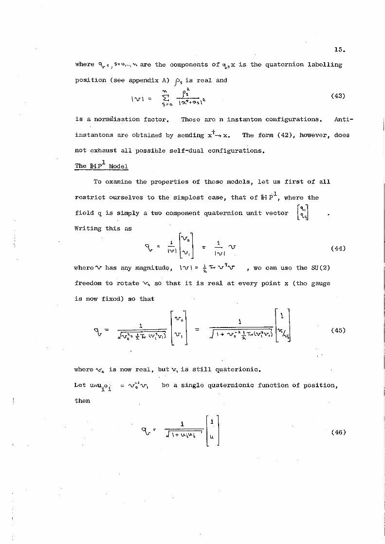
where ~ ~, s ... o, ... , "V\. are the components of ""' x is the quaternion labelling
position (see appendix A)
is a norm~isation factor.
fs is real :1.
fs
and
These are n instanton configurations.
(43)
Anti-
t instantons are obtained by sending x - x. The form (42), however, does
not exhaust all possible self-dual configurations.
The lH P1 Model
To examine the properties of these models, let us first of all
restrict ourselves to the simplest case, that of ~P1 , where the
[;·J field q is simply a two component quaternion unit vector ~~
Writing this as
where 'V has any magnitude,
'l
I vi
\ 'V I :: .l -r..,. v tv
"' , we can use the SU(2)
freedom to rotate v~ so that it is real at every point x (the gauge
is now fixed) so that
where v., is now real, but v, is still quaterionic.
(44)
(45)
Let U=U.e;~ ~
-I = 'V 0 v, be a single quaternionic function of position,
then
(46)

and now in terms of u
and
Thus
i =
u-t~J.I'-\.1.- a,...U.:u.. (.I+ I.' i.l.)..'•)
t. • .d ,.,.v.."'" ~" v..- ~ v v..;- dw- v.) ~ ~+ v-;, v..;. I'-
The equations of motion forJHP1
are obtained by varying "i with
16.
(47)
(48)
(49)
respect to u. They are most easily obtained by writing u out in its
components, then
l,
l)___ L ) ~-'" \,l.·t- Jv v. ~ - d-v v. ·~. d v- \A-~~
and, varying u., we find that ~
u + v..~v..t_)lj. (50)
to "'-'lz.lJru~).)...,.v.·~,') + Jp~,....v..~ dy.IA ~ ~rv..~- Jpa,..... u.ft 'd,..."'l. dpv.~ _ 'd }"\A~ dl<'"'~ 0 "'~ ~
- 4 }plv..,.,.v- .... ) ~!..dw-"'JU..,.u") )ru.Yt.- 'dr'ur.. 'dtJou~ )puj~ \.)+V.t,U.Q. \
-:::: 0 (51)
The 0(5) cr- - Model in Four Dimensions
~. 1 Just as for .~ P in two dimensions, where there is a correspondence
with the 0(3) <S ""model, there is a similar correspondence between ll-I.P1
[301 in four dimensions and the 0(5) .a -model · ·. The 0(5) cr -model has
fields which are real, five component unit vectors, ~l"JC.,, .. ,~~) with <PTcfJ:::- 1.
The <P rotate under global 0(5) rotations, and the Lagrangian density
takes the following form,

17 0
(52)
Where cp c.. I a=O 1 0 0 '4 are the components of 't and r 1 v 1 Q.. and b are summed
over. The topological charge density is
(53)
If we make the following identifications 1 for '\ 6 lH P1
(54)
where i=0 1 ••• 1 3 and the entries in the 2x2 matrices are themselves 2x2
complex matrices, then
<1\-::: 0... \)..~ ¢4- I+ \.A.~\J..~ -l + I.A~ \).~
' - I.A ~ "'"' (55)
\J.~= ¢L I- </>4. 9..
\.A~ lJ.}:::: -- \ +ll\~\,1\·~ -:::-
I + </;4 I + c{l4- I ;- <Pt..
where again i=o 1 ••• 3 1 only, and
(56)
Now substitution of (55) and (54) into the IH: P1 L;agrangian density 1
together with <J\ <I>~ -= I- <P: "::::? <j))» cf>~.,- </>z),.. ~4 )i=o 1 ••• 3 1 shows that these
Lagrangians are identrital 1 with').. =4.

18.
Similarly, writing the l-IP1 topological charge density as
d,v-V..o ... a.,-\A.o
= !)__ ~Jl'VfO' hl ~\ + v-~u;,) 4 (57)
a""v-~· •• ~ IS V.'l
one finds, usingfue properties of determinants, that this is identical
to the 0(5) <!"-model topological charge density. 1 Thus the i-1 P model
corresponds to the 0(5) cr- model in a similar fashion to the way «:: P1
corresponds to the 0(3) cr- model.
Instantons in IH p 1
In the light of ([; P1
models, where solutions are given by w(x1
,x2
)
being a function of either x1+ix
2 or x
1-ix
2, but not both, with
isolated poles and zeros, one's first guess for solutions of ~IP1 might
be
f (58)
where x = x.e. is a quaternion, labelling position, and p is a real l. l.
constant, with dimensions of length. Indeed, this satisfies the
equations of motion (51). It is in fact a self-dual solution, since
+ i-~ )J- .Q, 'V - .Jt,V~}/"
f~ ( \+ '~''l.r'l.)~ (59)
~i "'\.(.+)o. c:ro-y-v
f \.. I ... ,,., '1.; r it ) !1.
when is the self-dual 'tHoof t tensor (see Appendix A).
A more general solution is
(60)

19.
where a1 and a2
are constant quaternions, with dimensions of length, and
s is a real dimensionless constant. This is also self-dual, since
(61)
-1 ll.. <.::t.-t+o..')..)t-:1 l~~-'-~~-~viL! )~:x . .'~"t-o..~) \s-v...\
l.\+ IJ,.'-"''- ') :l.. (62)
which is ?gain manifestly self-dual. It has the same topological
charge and action as (58) since it is merely a conformal transformation
of (58).
The topological charge of (58) (and so of (60)) is one, since
= 1
"R '3 ).lkv.. ~ E> .J;W.... .p
t\+ R7r'l. y~-
(63)
where we have used polar co-ordinates (~,e,.P,~ ) on ~4, with R2 = 1x1 2•
Equation (60) is, in fact, the single instanton in Jackiw, Nohl and
Rebbi' s. . [44') 1
construct~on , and, noting that if u(x) is a solution of .IF-I P ,
-1 then u (x) gives exactly the same L.agrangian density and topological
charge density and so is an equivalent configuration, (58} is seen to
be simply the 'tHooft single instanton.
1 Again, guided by the CP model, a natural choice for a possible
two instanton solution might be
(64)

20.
However, we find that this does not give a self-dual field, nor
indeed does it even satisfy the equations of motion (51).
A more general configuration would be
\.A.= (65)
with a and b constant quaternions. One can try varying the values
of a, b and p to see if there are any values for which they make the
action stationary. Without loss of generality, we can move the origin
to (a+b)/2 and rotate the time axis so that it passes through a and b.
Thoo a = -b is real. Now let us see how the action varies as a function
of the dimensionless parameter a/f, and how it compares with the topological
charge.
With (65) and a = -b, real,
giving
?.. 'l.. L l. where t ,. ')(.. o , ...,.. = -:><. ' + "':1. t- Jl -.. • Then
(66)
(67)
l.l+ [ lt +O..l'l.. +....,.1.1 \:.lt-o. \ t+....,.'l.1 ~It f
(68)

21.
(for details of the integral, see appendix B)
(69)
giving
't \C>
\biT+~ IT ( 70)
where t =-\.if , ;::;. "~If , 0.."' o..1f are dimensionless. (For details of (69)
see appendix B) •
Upon performing one integration in (70) (see appendix B) we obtain
~ 2.. \00 S = 1 b 11 + go '1r .) 0
(71)
which was evaluated numerically, see graph on "(;he next page
A measure of how close the configuration (65) is to a solution of
the equations of motion is given by
(72)
.....,1,.
with self-duality for I(o.. )=0 • .-...?..
The graph of I ( o. ) as a function of
....,.l.
~ is shown on .the next page
We see that the action montonically approaches its lower bound in
the two instanton sector as Furthermore, it approaches this
'I. limit very rapidly, being within 0.7% of it for a= I •
a two instanton solution, only in certain limits:
Thus we have

r j ~ "
I / I
/ ;· ~/~
~.,/
----~----" r-~~--· -t----.. 0

22.
(i) f fixed, 0..4oo i.e. the instantons are of finite size, but
~"-I ( a ) represents a repulsive interaction which sends them infinitely
far apart.
(ii) a. fixed, p-c i.e. the instantons are at a finite separation,
but their size shrinks to zero.
Case (i ) has been analysed, in a slightly different form, by Neinast and
st~roJ52} I am grateful to Werner Nahm for pointing out the interpretation(ii).
Nahm has coined the phrase "virtual stationary points" for such
configurationJ51~
One expects that such configurations would contribute to functional
integrals, since the action is finite, and therefore must be taken into
account in any attempt to quantise SU(2) Yang-Mills theory. However,
it has not proved possible to perform the functional integral, using
(65) with~~~, as a stationary.point, due to the singular nature of
the fields.
Indeed, for any finite integer -Y>..:;:. l , the configuration
(73)
has finite action and topological charge k, and so such configurations
will contribute to functional integrals. The action and topological
charge are most easily calculated using spherical polar coordinates.
~
where 12.. ::-y:"""J:"" and -!R::: C«>9>~,+~ <1!~'1\1"-tQ.. +~ '{>J.v<.,.,.l\r-4..?. and )
o ~ i2- "-. oo , o ~ ~ ~ 'IT , o ~ ¢ .::S 'l"r > o ~ ~ ~ ?...IT .
Since *'-"-'"- ~ we have de Moi vre' s theorem for quaternions, - -.L~x2. I
(74)
(75)

Then, with (73)
~~-1
l\2-/ (' l J:»m, ~ &
[I+ '-·p .. '/f )"~r·
:1.,·~
~ ~ l P..tr) ~ ~ ~
c I + t.?tp )~~ r· :t. ~ \.. ~~r )').. ~ .AIM.~ e
L \+ !J-tr Y~r·
l..~ ~ cF-;f) ~ '),.~e~ <fJ ~
\:. \+ !.,.1-tp '1;1.~ y·
etc,
With (75) one obtains the action and topological charge
23.
( 76)
(77)
The action is manifestly finite, for fintte k, since the integrand
in the last term is bounded in the finite region of integration, However,
the only one of these configurations which is self-dual is k=l. It seems

24.
probable that a similar situation will arise for k)2 as did for k =2
i.e. that self-duality will be achieved in the limit of the instantons
becoming infinitely. far apart. The calculation has not been performed
for general k, however, due to the complications arising from the
quaternionic nature of the variables. Configurations of topological
T charge -k are obtained by sending x~ x or indeed changing the sign
of any odd number of the components of x. All of these configurations,
therefore will contribute to the functional integral, though it is not
clear how to perform the calculation.
Excluding the singular configurations, it appears that HP1 does
not have the rich topological structure of <C P1 • However, Gursey et
a£37: Jafarizadeh et at
451 and KafieJ
46] have shown that, for u(x)-=x~~~
f ~IP1 to gravity, with the metric coupling
(78)
gives a self-dual solution of IHP1 , in the curved space -time described
by (78), with winding number k. In the next chapter, it is shown
that this can be done for any quaternionic polynomial of degree k,
and in the process a method is developed for constructing a self-dual
SU(2) Yang-Mills field over any space-time with a given metric.

25. CHAPTER 3
MULTI-INSTANTON SOLUTIONS OF ]r.ipl IN CURVED SPACE-TIMES
The problem of finding multi-instanton solutions to liiP1
, as
exemplified in the last chapter, has been circumvented by Gursey
~TI ~~ . ~~ et al , Jafarizadeh et al., and Kaf~ev • These authors extend
the conformal invariance of the Lagrangian (2.49) to invariance under
general co-ordinate transf0~ations by introducing a metric,
and constructing HP1 in a curved space-time. In this way they
construct spherically symmetric, k instanton,~P1 configurations. In
this chapter, their method is extended to more general, non-spherically
symmetric configurations.
1 The Lagrangian density for 1E-:I P in curved space-time 1 with metric
~ )J-V 1 is taken to be (in naturalised units/~i.:.c = 1).
(1)
where
(2)
Here~ is a cosmological constant andK=4~G, while G is the
gravitational constant. R is the curvature scala.r obtained from ~)JIV
(the conventions are those of referenc~411except that here the metric
has signature (++++~, and g = det g • J..l'\1
By varying the metric in L, we obtain Einstein's field equations,
(3)
where the energy momentum tensor for the field F is T given by p..v p-V 1

26.
Since the energy momentum tensor is traceless (g~vT =0), it p-v
is necessary that R = 4 A in order that equation (3) be satisfied.
Thus 1 if the lH: P1 are the only fields present 1 apart from gravity 1 a
cosmological constant is necessary in order to satisfy Einstein's
equations (unless the metric is such that R=O).
The expressions for the dual of F the IH:P1 action and the )"'V'
topological charge are modified from the flat space-time definitions.
Define
+1 for any even permutation of 0123
-1 for any odd permutation of 0123
0 otherwise
(5)
for any curvilinear co-ordinate system. Then is not a tensor,
but a tensor density of weight -1.
Thus the dual of F~~ becomes
The correct tensor is J.. c Y'llo>..(1 Jf
I ?..
(6)
So the lH P1 action and topological charge become 1 respectively 1
Here the integration is over the manifold described by g }"\J
indices are raised and lowered with the metric.
( 7)
(8)
and all Greek
Writing the RP1 field te·nsor (2) as a Yang-Mills field, derivable
from a potential, as in (2.34) we again define
I ')...
v..:•~J..I'V-- ~yV-'t\A..
( \ + \);~ V-\, )
(9)

27.
i.e. (2.47) is unchanged by the introduction of a metric. The Euler-
La,grange equations obtained from (1) by varying AM- are now
i>.IJ' -t~ r"-'\)~ = ~ L ~}1\v, A11'-1 '
By restricting ourselves to A of the form (9) 1 any solution of (10) Y-
is a solution of H p1 •
(10)
. [3 7 45 46] t \ fz_ The authors ~n references 1 1 show explicitly that u.. "' \-:x.'f' J
is a solution of (10), with topological charge k, provided that the
metric is of the form
~t av-l~t)Ytdv(~)~+ ~v~~t)~Jf-l"l~)~~ l' + { "1k- (~)~~~)~ J (11)
where f is a constant, with dimensions of length (i~37 , 45 and 461 p = 1).
This metric describes s4 wrapped round itself k times, and the resulting
field, Fpv is spherically symmetric. In what follo~s, this result will
be extended to field configurations which are not spherically symmetric.
Considerthe metric
.f'l. t;.... (. a~"'\..L ~'II u...t)
'l.. (.\+~;.\.1.\., )'). (12)
where u is any quaternionic function of x, which is differentiable)so
as to give a non-singular, continuously differentiable metric, ~ JI'V •
The requirement of non-singularity of the metric excludes the meron
configurations of de Alfaro, Fubini and Furla~2 ]in which
(13)

28.
4 gives a meron via (9) (though their space-time is S not that given
by (12)). To see why this is excluded, write x in spherical polars,
as in (2.74)p giving
0.4)
so 'a'p.:v = 0 for all 1> and det g = 0 everywhere.
For well-behaved u(x), ~etric (12) and potential (9:), equation
(10) can be simplified in the following manner. Construct Vierb'eins
for the metric (9)
(15)
in terms of which
(16)
Here, as in everything that follows, Greek indices represent curvilinear
co-ordinates· and must be raised and lowered using the metric, while
Roman indices label locally flat co-ordinates. Since the metric has
signature (++++) there is no distinction between co-variant and
contravariant Roman indices.
Now construct the quaternions
(17)
Thus
(18)
(19)
Using the properties of quaternions, given in appendix A, (18) and (19)
can be written as
(20)

29.
(21)
Then, using the commutation properties of the "1. symbols (A.l3) and (16)
the left hand side of (10) becomes
, Now consider the ·1d't. hand side of equation (10)
dy-\~ ~t"f'1-\IO"\dr\N-t d1S"\.L- 'da-v.+ ~r"'\~+v-·"\.lt,),_~
d .v- ~ ~ ~Y~ '1-Y(J ( 'dr v..;- do-v-- ilo-~ Jr \JI )~
= 3,..~~ ~Jvl~~vcr l3ru:'"~crv..-i7a'v..-t Jel.l)1
\__ I+V:~~·L )
?,_ ~F)"VdMti+V.~\).·~)
l.\-tv.j\.1..~\
where (15), (16) and (21)have been used. Thus we see a remarkable
cancellation between the non-abelian term in the equations of motion
(10) and the derivative of the denominator of F~v, reducing (10) to
(22)
(23)
(24) now, use
(25)
for any Here a semi-colon denotes
co-variant differentiation with the connection induced by the metric.
Hence (24) becomes
(26)
since the metric is covariantly constant.
The Christoffel symbols induced by the metric are
(27)

30.
af~a' '-<~)..'. u. \.
\,\+ v-~v.~)'). l. c ~f \J.-)6" I.A.~;. 'o~ v,~}~v.;_- ~fO" V.i, d.v-IA;_)
<._\-1-IJ..~U.\-1..).
Then, writing (26) as
(28)
0
it is straightforward to check, using (15 1 (16) and (27), that (28) is
identically satisfied. Thus any u(x) 1 provided it gives a continuous,
differentiable, invertible metric, via (12), will satisfy equation (10).
This is an extension of the work of references f 37 ' 45] 1d. [46Jwhere only an t R ,
the special cases u = ( -~ ) 1 _ for integral k, were proved to satisfy
(10), using spherical polar co-ordinates. In the more general case,
however u(x) could, for example, be a quaternionic polynomial in x of
the form
(29)
where a., b~ i = l, ••• ,k are quaternionic constants with dimension of ~ ~
length and 'X (x t ) is a polynomial in x t
to k-1. Polynomials of the form (29)
been shown by Eilenberg and NiveJ281
of degree less than or equal
+ \ Yt are homotopic to l t;X./t 1 as has
In fact, one can go much further and prove that the above construction
for F in the metric (12) is (anti) self-dual. !" \)· The proof is quite
simple and proceeds as follows. We have, by definition
(30)

31.
using (21). Now, from the properties of determinants
where
and the sign ambiguity emerges because (16) only determines det~. ~}-A.
up to a sign. Now, putting (31) into (30) and using (16) yields
(31)
(32)
(33)
. t-) Q. • t. lf d 1 . ( . ) s~nce "'\. . . ~s an ~-se - ua ~n ~,j • '\;~
If, instead of (19), F had p.v
been defined· as
(34)
the role of the <±) sign in (33) would have been interchanged, since
is self-dual. Using similar methods, involving the properties
of theL symbols and contraction of Vierbein indices, the action (7)
and topological charge (8) are found to be
(35)

Q::::: + 'X lV~ 1- .Jlf<k.Q..-~)
lr'l.ft.~-
32.
(36)
Note, in passing, that the analysis from equation (30) through to (36)
does not depend on the Vierbeins,~~~ being of the form (15), and will
hold for any metric, 0~~~ not just those of the form (12), provided
F is of the form (21). The potential A~will not be given by (18)
Thus, given any metric, ~ p.v , an (anti) self-dual
r\) in the general case.
SU(2) field tensor can be constructed using (34) (self-dual if det(R~y)
>o). The only degree of freedom between '1--,..v and Ff-'V is that of y, a
scale. This is only to be expected since Yang-Mills is scale invariant,
whereas gravity is not. In general, however, the exist e nee of a
potential, A , for a field of the form (34) is a more complicated ·}J--
question, and will be deferred until the next chapter. For the moment,
let us restrict ourselves to ~P1 , where the Vierbeins are of the
form (15) for.which the potential is given by (9).
To calculate the topological charge of the configuration (29)
use will be made of the theorem of Eilenberg and Nive~8Jthat the
polynomial given by (29) is homotopic to \:'"'"!\)ttL Since Q is a
topological invariant it is invariant under homotopic deformations
of the fields and it suffices to calculate Q for v.. ::::: (X-t/p l 1\ and this
th will be the same as that of a general k degree polynomial. The
calculation proceeds as for chapter one, except that now the metric
must also be included. Writ~ (c.f(2.74)).
Then the metric (11) is diagonal and is given by
(37)

33.
'"-
:\.~~?... ~. 0
ca- }/'V - ('R;f) ~:1. 'R:t (38)
I_\+ \_\2-/~ )~1(1. f -R~:l..~e
0 12-~~~e~ cp
(39)
In order to see what space this metric describes, let us make use cf
the invariance under general co-ordinate transformations of the action
obtained by integrating (l)o Since the whole of the above construction
is invariant under general co-ordinate transformations, let us simply
('XIt) choose co-ordinates '\ p '=U 1 then the metric (12) is 1 locally, just
the standard metric on s4 , obtained by embedding s4 in ~ 5 and
using the standard, flat metric in 5 ~ , except that now,
(40)
where
(41)
34.
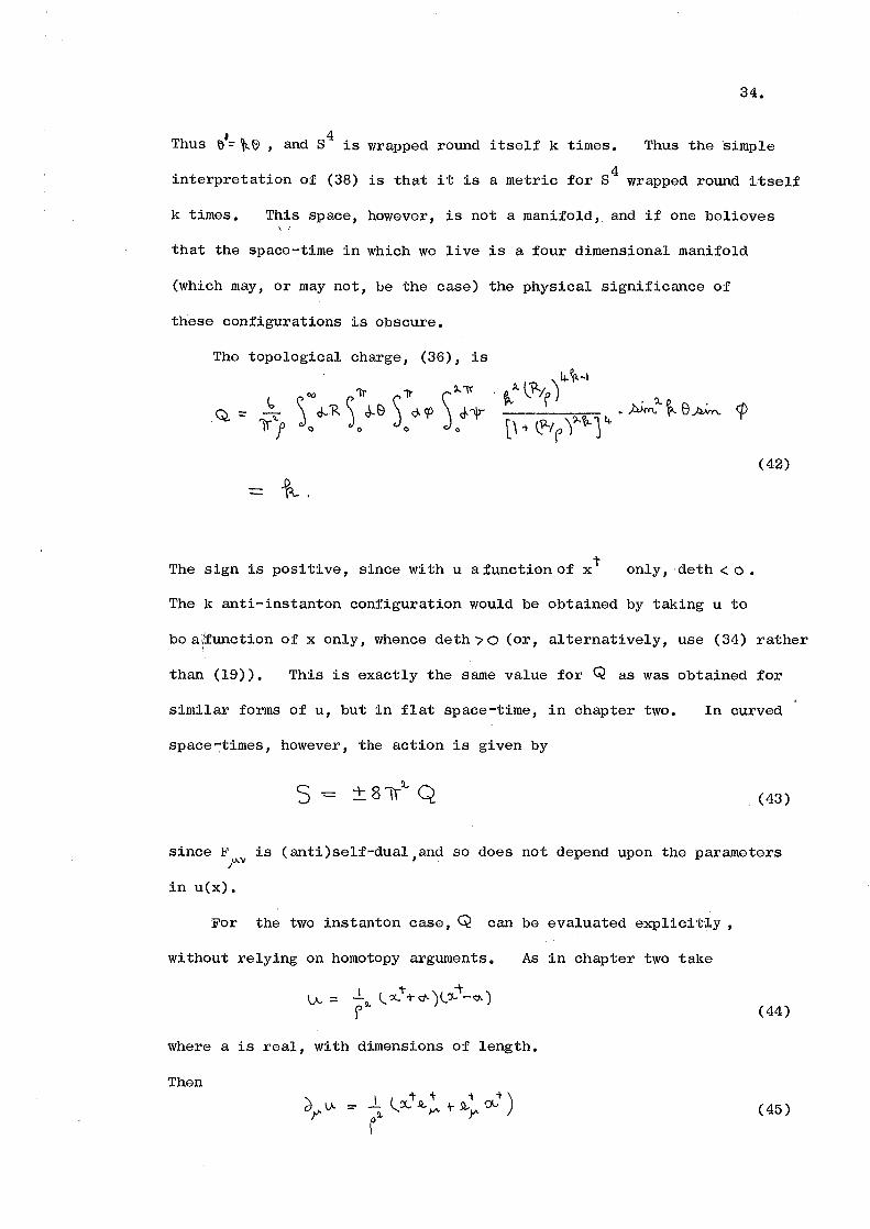
Thus fJ1= ~0 , and s4
is wrapped round itself k times. Thus the ·simple
4 interpretation of (38) is that it is a metric for S wrapped round i.tself
k times. This space, however, is not a manifold, and if one believes
that the space-;time in which we live is a four dimensional manifold
(which may, or may not, be the case) the physical significance of
these configurations is obscure.
~.
t The sign is positive, since with u a :function of x only, ·deth < o.
The k anti-instanton configuration would be obtained by taking u to
(42)
be a.:function of x only, whence deth I' o (or, alternatively, use (34) rather I
than (19)). This is exactly the same value for Q as was obtained for
similar forms of u, but in flat space-time, in chapter two. In curved
space~times, however, the action is given by
(43)
since F is (anti)self-dual,and so does not depend upon the parameters rv in u(x).
For the two instanton case, Q can be evaluated explicitly ,
without relying on homotopy arguments. As in chapter two take
(44)
where a is real, with dimensions of length.
Then
(45)

35.
and USing CO-OrdinateS ( 1) 1"" 1 e 1 * :L '1. 2. 1 ) ) where "' =: \. ':lt, + :X.1.. +- ?l.a with
diagonal
(46)
0
So ,fg is easily evaluated to be
\ b \. t.'-+ rr") -\; 'l.'\l.. J:J.Jvv..... <P
- fl.rd._l+ [l t-to.)'"+~'- 1I.lt-o. 1').+-r"'l /p4-14-(47)
Putting (45) into (36), with a posttive sign, since (44) gives a self-
dual field, yields
Q= (48)
This is identical to the topological charge for the field configuration
(44) in a flat space time, which was evaluated in chapter two (2.68),
and appendix B. There it was shown that~= 2. In the presence of
..__:t gravity, however, the interaction between the instantons, I(~ ) in
equation (2.72), is exactly balanced by the gravitational field,
represented by the metric, making S independent of 0. = o...; f ' so

To summarise so far:
Although
F y.v -dyVvi d...,"'- -J...,v.:t ~,_..v...
l\ +- u.·"v..~ )l.
does not solve the equations of motion in flat space-time, for u(x)
36.
(49)
an arbitrary function of x or xt 1 it does if we introduce a gravitational
field
\:=...- l d)J-~ d-y \A.)
(_\ + \At,U.·~) :t
th t In particular, taking u to be a k degree polynomial in x (or x)
(50)
yields a self-dual (anti~self-dual) field configuration, with topological
charge .±_k.
Once the space-time is chosen, i.e. the metric (50) is given, there
is only one degree of freedom in our choice of F that of the scale yv'
f· It is natural to ask whether or not it is possible to extend the
above idea to a more general F , e.g. if we take yv
(51)
and F of the form (49), with u an yv
th• arbitrary, k degree polynomial,
then is F self-dual in the space described by (51)? yv
In general this could be a difficult question to answer, so let
us first of all consider the simpler case of the instantons being
strung out along the time axis,
(52)
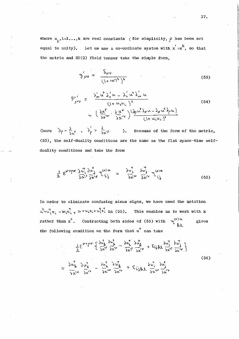
37.
where ai, i=l ••• , k ·are real constants ( for simplicity, _p has been set
I k equal to unity). Let us use a co-ordinate system with x =X , so that
the metric and SU(2) field tensor take the simple form,
(53)
(54)
(here 1 ) . Because of the form of the metric,
(53), the self-duality conditions are the same as the flat space-time self-
duality conditions and take the form
(55)
In order to eliminate confusing minus signs, we have used the notation
t ~ ~ t~ U..""''-'->.-1!.;, =1/..i..~;, ~ v.=-v.~~?.~=ui.~?..~ in (55). This enables us to work with x
+ rather than x • Contracting both sides of (55) with
+ the following condition on the form that u can take
=
gives
(56)

38.
Equations (56) represent nine differential equations which u+ must satisfy
for (54) to be self-dual.
where
+ To check whether or not (52) satisfies (56), rewrite u
I .-t = "'~ L I ~-1 I \_ vv - _,._ ' Y.J 'tt.-1 :X. + 0 0 0 + t>, 'X. + I? <::J
b-t>,_ = 1
I
as
(57)
(58)
i.e. bk-r is the ~ymmetric product of r ais (b real). r
Using spherical
polar co-ordinates
we have
Thus
1' v... ""
J ':X-():::
I "J...,:::
"):.:
~ "5J b,..Rrrl~<'V"tJ.J.~~'T'tJ) <'('"'O
0c~ = ~<!> ~~ R\t.~ ~0
'Y--~ -= ~ q ~'"'\' R~ ~ ~e
(59)
(60)
(61)
(62)

39.
I
1 ~ I 'l. I \ 'l.. I \ 'l J !,l..ft [ l~o l + l:L1 l + \.:.X.'l..j + t1--o l
e =
¢= (63)
Now it is a straightforward, though tedious,application of the chain rule
to check equations (56). One finds, using (61), (62) and (63),
1 oi.Ao
= 0~~
~\). "\ ""
'()':1..' I
1 /.liM.~~ ~9..-t 21 ..... b'T R"" c.c-0l~- .... ~ e f;l~i. ~
() v:~ - ~
~ 0..~
-r 1 .l ~'J..cp c..e-6~'-~>-~-~'lv) 22 b ... R"'~~ e R.Vt.~~e <T
==- ~R~ ~'-<P~y ~,.,b,.... Rrr <:.¢-OL-'b--...-)9
+ 1 • L c..o-':> 'l. 'f> .J:V..m. 'I.V" + ~'1-y) '2 b,... R"' ~rr e
p.:~· ~ ~e ~
Ju.; I . ~ . 3.,.'6 ::- li 12--~ ~ "' ~ 'T b ... R. ~<.:~-.... ) 0 :::
'dv.."~'2. ::: ~ o • .J.W.,. <P co-o y ~ ""b~ R-.-~ l~-~) 8 '))')(.~ P. 'j2-_'T' ,...
"lA"to ,i I <} <>"'"?. • • I. ,.... il:1-~ ~ - -r,..'o., ~.J.l.Jv.n.~~y~ rr r.>IT'R ~L~-....-)&
dl).i -I':::
';\::>~')..
+ ?>v..'l. == ~ cp...., '1' ~~ 2 b,_ R .... r ~ C<J?\f4-...-) e- ~'T"e '2. ~-:1-.: 'il..~ ..,. '\. ~ AM-.. ~e ) (64)
~ "'~ ::: ~ <P C,.(y.) ~..AiM. '1\r- 2 b R'" \. !!:. <:.oJ.> (.~-..... ) \9 - AW.""" 0 "L d'Y--{ \2...'1L. ,... ,.... Pz_ ~ ~\9)
au.~ = dlA~ = ~:~.cp.J.lk...~~"\f Z \,,.. R""\~~l~-..-)fl-~ 1 J?l~ ';)')(.~ ~ ..... ,.. ~~{})
~

40.
It is convenient at this point to define the three quantities
(65)
~=I
Now let us put (64) into the nine equations (56). For example, consider
(56) for the case y--~o, y-,t,ll.~o,~==l (the analysis for the other eight
cases proceeds in a similar fashion). In this case (56) gives
;) \A.: il v...i d ~~ :>Jv-\ + \~ \!-~)~ + + ~
~o.:t oo; _ ~ •i '"' J (dtk~) +- J_ - 'cJ-:J..' d I - -cl::f-~ d:J..: ;:h{ o:x.; d':X.; (} 'J.~ 0 ::1--, h~ ~'JL~
:::: 0.
Using (64) and a little trigonometry, (66) becomes
'l.. 'l.. 'l..
C~-Til+ S~:::. o.
Using the forms for Ck. T and Sk in (65), (67) is I k
(66)
(67)
Since (68) must be satisfied for all values of Rand 8, each term must
vanish separately, giving
(69)

41.
for all e d 1 1 k an r,r = , ••. , . This can only be satisfied if b =o;r=l ••• , r
k-1. b0
is thus the only arbitrary constant, since bk was fixed to unity.
(Changing bk amounts to changing the scale, i.e. changing p ). The only
function u(x) of the form (52) that is allowed is thus identical to the
function used in forming the metric (51) modulo an additive constant.
The freedom between F p-v and "J J"V carried by b 0
amounts simply to a
translation of the origin of the x' co-ordinates. In general, a full
conformal transformation of x' will leave F self-dual, i.e. take )-'-\J' '
-1 -v- =(a u +b) (cu +ct' ) , where a, b, c and d are constant quaternions,
then F of the form (49), with u replaced byv will be (anti)self-dual )"-\!
in the metric {50). But this is the only freedom between F and ~ .. v• p.v r
We cannot perform conformal transformations on the original, unprimed x •
In this chapter, the work of reference~37 ' 45 and 46] on lt--1 P1 models
in curved space-times has been extended from 0{4) symmetric solutions,
to solutions with no particular symmetry, u(x+) any
+ polynomial in x • On the way, an interesting result was uncovered,
the self-duality ofF of the form (34), in the background metric (16). )AV'
1 This result is in no way dependent on the~P structure of the fields and
is a general result for any SU(2) Yang- Mills field. However the existence
of a potential for F constructed from (34) is, in general, a tricky problem. y.,v
In the remaining part of this work, ~IP1 models are abandoned, and the
more interesting problem of SU(2) Yang-Mills in curved space-time will
be examined. The analysis will be based on equation (34).

42.
CHAPTER FOUR
SELF-DUAL SU(2) FIELDS IN CURVED SPACE-TIMES
I
In the previous chapter,il~ fields in curved space-times were
considered. These fields are a special case of SU(2) fields, namely
SU(2) fields of the form (3.2) and (3.9). In this chapter (3.2) and
(3.9) will not be assumed, but more general SU(2) fields will be
examined, in the presence of a gravitational field. First let us
summarise the salient formulae for SU(2) Yang-Mills coupled to
gravity (3.1), (3.3), (3,4), (3.6), (3.7), (3.8) and (3.10). The
action is[lSj
(1)
The quantities are as in chapter three, except that e, the Yang-Mills
coupling constant is no longer taken to be unity. The integrals are
over the whole manifold, M , endowed with the metric,"} J-'V • The surface
term is only present if the mardfold has a boundary, or is non-compact
(for details, see referencel3~). In what follows, only compact
manifolds, without boundary will be considered, and so the surface
term will not be present.
By varying the metric in (1) we obtain Einstein's equations
where the energy momentum tensor, T , is y..v
F is derivable from a potential (A y..-=== -1. <Jo.- A:_ ) y.-v ;
(2)
(3)
(4)
43.
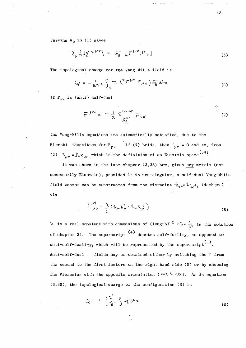
Varying Ay.. in (1) gives
(5)
The topological charge for the Yang-Mills field is
(6)
If F~v is (anti) self-dual
(7)
the Yang-Mills equations are automatically satisfied, due to the
Bianchi identities for F y-v • If (7) holds, then T}A\1 = 0 and so, from
(2) [54]
R]J'v =A ~1-'v' which is the definition of an Einstein space .
It was shown in the last chapter (3.33) how, given~ metric (not
necessarily Einstein), provided it is non-singular, a self-dual Yang-Mills
field tensor can be constructed from the Vierbeins +t_JJ-= ~~f".e-i. (deth/o)
via
(8)
1\ is a real constant with dimensions of ( length)-2 ( '"\" \ in the notation f
of chapter 3). The superscript (+) denotes self-duality, as opposed to
(-) anti-self-duality, which will be represented by the superscript •
Anti-self-dual fields may be obtained either by switching the t from
the second to the first factors on the right hand side (8) or by choosing
the Vierbeins with the opposite orientation ( c:kd ~ <:.o). As in equation
(3.36), the topological charge of the configuration (8) is
(9)
44.
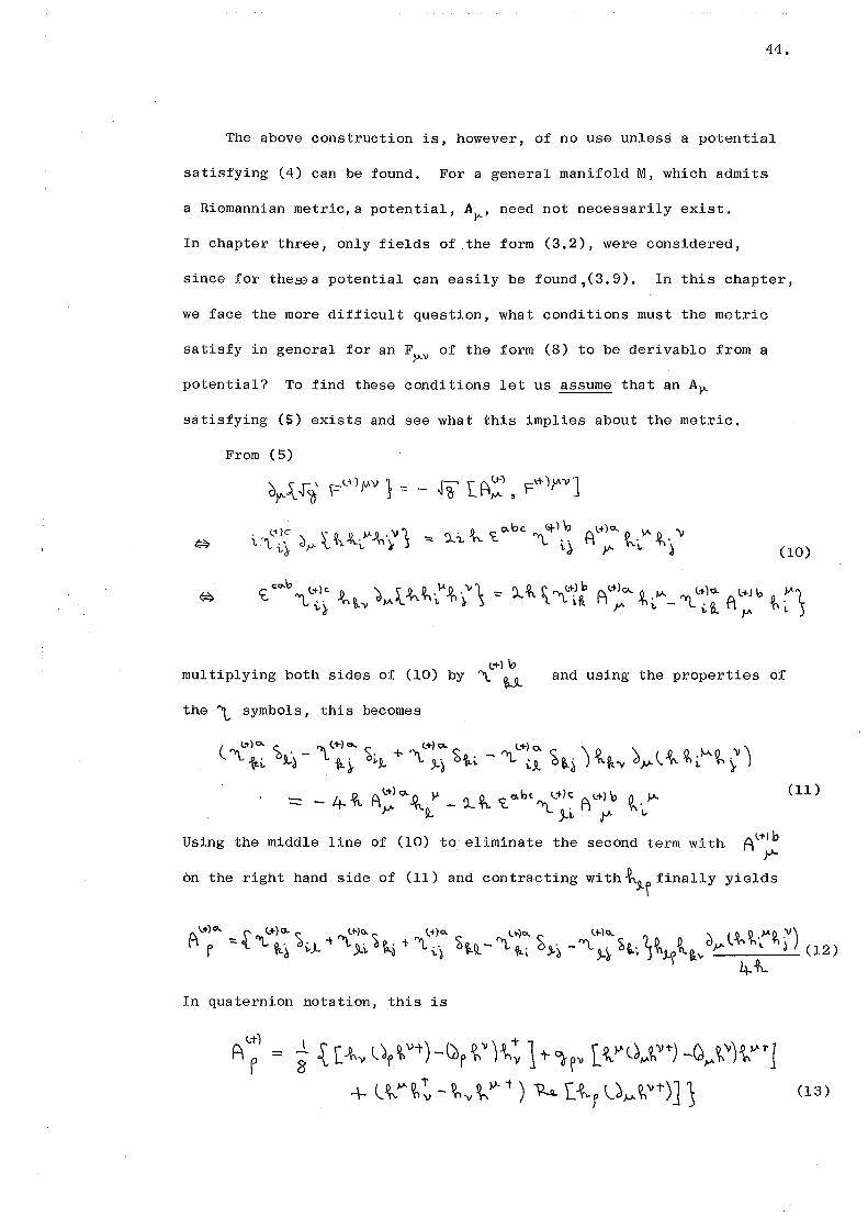
The above construction is, however, of no use unless a potential
satisfying (4) can be found. For a general manifold M, which admits
a Riemannian metric,a potential, A~, need not necessarily exist.
In chapter three, only fields of the form (3,2), were considered,
since for therea potential can easily be found,(3.9). In this chapter,
we face the more difficult question, what conditions must the metric
satisfy in general for an F~v of the form (8) to be derivable from a
potential? To find these conditions let us assume that an A~
satisfying (S) exists and see what this implies about the metric.
From (5)
(lO)
(.+) \? multiplying both sides of (10) by ~ ~~ and using the properties of
the ~ symbols, this becomes
(ll)
Using the middle line of (10) to eliminate the second term with
on the right hand side of (ll) and contracting with t.9-f finally yields
In quaternion notation, this is
t~ T Af = 8 ~[-t~t.af~v-t)-Cdr~")~v 1+"0'~v L:~~.~-'laM~vt)-~, ... t\l)~vt-1
+ l t.v.~:- ~v ~))- t ) I2.A. [ {.f \.J,.._..~'~~"~-)]} (13)
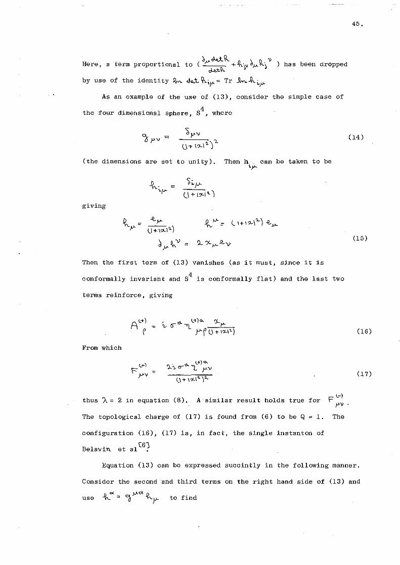
b J.d~ \ () '\) Here, a term proportional to ( J.l' + t.~v o,v. n·} ) has been dropped
~Q-.
by use of the identity ~ c::kk. 9..;.}"- = Tr k ~ ;.,fl"
As an example of the use of (13), consider the simple case of
the four dimensional sphere, 84 , where
(the dimensions are set to unity). Then h . can be taken to be i.y-.
giving
~)J-
u + \o'--1'1.)
d ~ \) ::: 9..- 'J(. ........ ..Q..)) )J'
Then the first term of (13) vanishes (as it must, since it is
conformally invariant and 84 is conformally flat) and the last two
terms reinforce, giving
A<..-t-) ct. ~:+ 1 0.. ':}._
-= '\., 0 "ft. }-'-f Y'f 0 + 1~1'-)
From which
<..+) . L+) o.. ')..-., a-0.. '1. J-AV r y.v :::
(,_\-t- \')(.\9..)'l...
thus A= 2 in equation (8). A similar result holds true for F~~
The topological charge of (17) is found from (6) to be Q = 1. The
configuration (16), (17) is, in fact, the single instanton of
BelaYin et alC6)
45.
(14)
(15)
(16)
(17)
Equation (13) can be expressed succintly in the following manner.
Consider the second and third terms on the right hand side of (13) and
use to find

'1-fv [t!""\.d_.,._~vt)-l'd_v.~")t_; J +l~~~-!hv~J.At) 14-l~p~M~lltJ
- [~~,.,..~;~_(ciJ.A-~pl~+] +-l~'""tv+_~v~}A+) Rt.l~r'd.Mq._~)
+ l~~: -~ot~t)~rv d.v 'tva{+ l.v-'~:-~ ...... ~t) R....(~p~~ Jd""'CJ-v~_
Since ~vpd~-"~"o(l::"-'d,..~..,.r1p.o. and Re(~p~:) ==~fO(' the last two terms
on the right hand side of (18) reinforce to give
<tpv [ ~'-'a.v-~vt_c~}'-~'~) ty-;1-+ \..V~~-~.,~Mt) ~ U'"P ~y.!hv t)
:::: {;"df"'~tf -~J..'-!(.,_~y.+ + lt."'q.,v+_~v~v-t) ~ \.~fd);I.Q_:)
- ~ l~).A~v+_ ~"V~Y.t) d_,v.VQ-yf.
Now, the last term on the right hand side of (19) is
Where
-l~~~v+ -~v~v-+)ld~~"P- J-..<a~-'\ l == ~l~J-A~V-t_~v '?-."""t) T}r.)vp
l' T'o! .)}- ) v p -= ~ )J-d. "V?
~ ~D . and 'vp are the usual Ghristoffel symbols for crf"Von M. Equatl.on
(19) can be further simplified, since
\_~t"VT_ ~"V~T)d,v-%>-p -=:: l~l-'~V't_~Vift) dy.l.q.,i.v~-\.f)
:::: (_ ~>J- ~ '\l't_ '?-,..., ~M t ]CJ ,_..<?.,;_"¥) ~ ~p -+ [~}A JJ.A ~; - <,_)_..,. ~f \ ~~tl
-::: \.~v.~._v+- ~ 'v~)A+) ~ <J"r a~-'~~ ) + r ~ d.J.A ~;- Q"" ~P H.; .... tJ .
Where, in the first step, use has been made of t_V~-\.v"" ~~ So
the first two terms on the right hand side of (19) are of the same
form as the third, reducing (19) to
~pv '[~ dM ~vt_ ~""~v)V-11 +\..~Mt:- ~v~t) R.e. u .. ,p ~Mt\.lt)
- r~ ov"~'_~v~T l -pJA - 1..:: )J-n y- vr .
46.
(18)
(19)
(20)
(21)
(22)
(23)

l+) Putting (23) into the expression for A f ,(13), one finds
Denoting covariant differentiation of a contravariant tensor by
lt-) the following, beautifully simple, form emerges for Af,
i { ty. '- t_Y-;r">t- ~M;r ~~ 1 _L ~ l ~Y-. ) t 4- p- ,p
Where, in the second step, we have used ~ L t r l~)~1= 0, since ~ o<~
is covariantly constant.
47.
(25)
(26)
Now demanding than an FL+-) of the form (8) comes from (26) via (4) J"V
will produce a set of second order, partial differential equations for
the Vierbeins which must be satisfied for a potential to exist. Not
all manifolds will admit a metric which factorises into Vierbeins which
meet these conditions.
Before applying (4) to find these conditions, it is instructive
to stop and examine what is happening from the point of view of group
theory. In terms of the~ symbols, (26) and the correspondeequation for
anti-self-dual fields, can be written as
(27)
Now the spin connection for a manifold, viewing the curvature from
the point of view of an 0(4) gauge theory, is defined as (see Weinberg[6l1
p 370 and Utiyama [6~)
(28)

48,
Wherecr- .. =-a- .. are the generators of 0(4), satisfying the following l.J JJ.
commutation relations,
(29)
Since 0(4) ~ SU(2) x SU(2) as a group, so that the algebras decompose
the 4 x 4 rna trices <'S • • can be decomposed l.J
into the direct sum of two 2 x 2 matrices. A faithful 4 x 4
representation of SU(2) x SU(2) is given by
0 (30)
where each entry in (30) is a 2 x 2 subrnatrix. That (30) satisfies
(29) can be checked by direct substitution, using the properties of
the~ symbols. Note that (30) are complex matrices, and so, strictly
speaking, form a representation of SU(2) x SU(2) rather than 0(4).
Using (30) as the generators for an SU(2) x SU(2) gauge theory with
spin connection (28), we see that
::::
R'+l p
0
(31)
0
Which expresses the fact that the (anti) self-dual SU(2) potential (26)
is simply the spin connection, restricted to one of its SU(2) subgroups.
Equation (31) is identical to the starting point of Charap and Duff
[151 I though they restrict themselves to manifolds, M, for which the Ricci
tensor vanishes, in order that Einsteins equations (2) be satisfied,
without a cosmological constant, and the Riemann tensor is double self-
d lt491
ua • In this work, this restriction has not been made, and SU(2)
fields in an arbitrary ~JAY are being considered to see what restrictions

49.
must satisfy in order that a SU(2) connection, derived
from (8) exists. We shall consider Einstein's equations later.
A note on gauge transformations may usefully be inserted here.
The decomposition of ~~v into Vierbeins, equation (3.16), is not
unique, but only defined up to a local 0(4) gauge transformation
h. -4 0. jh. where 0. j E 0(4)(or 80(4) if we restrict ourselves to deth>O), and J. Jl 1. J}l J.
Oij can depend on position. A different choice of Vierbeins merely
(+) alters F obtained from (8) by a. SU(2) gauge transformation
JJ'"J
F (+) . ----=. g F(+) -l where ge.:SU(2), the SU(2) element obtained from O.j
)11-\1 g J. \1'-V
via the decomposition (30),
Now we shall proceed to derive a set of second order, partial,
differential equations which the Vierbeins must satisfy in order that an
SU(2) potential derived from equation (8) exists. From (4), (8) and (26),
one finds that
F;~ ==: i { d}o' \ ~f dv ~ft) + 'd)Jo \.~,_ ~ft) "Pr: + ~'}.~r+ d_,... l'f~
- av <__tf ci..,.~i-t)- Jv \.~'>.. ~i+)\';1"- ~'A ~r+ )v 'f~ (32.)
+l [~ il ~rt t ~ ~').,+1+..!.\~ a.i>?+ ~ ~a-+]r.'>-Lt- f JJ- ' "}., \1 '-t L I ..,. 'f' ' 'A . 11"\1
+ i [~A ~IS"\ ~p av~ft} \'; + i: L~ ~rt 0 ~Oit1-r'). \l{f' I ,)J" ~ :>., , ~ f}" I 01))
The commutators can be evaluated using the properties of the ~ symbols
(here the notation v~ \;~).~f) =~ !,._ ~,.,~~ -~r~\) is used - see appendix A)
I [ t_ 'd ~f+ ~ ~ ~'X t 1 · o..bc l'l)o. <.tlb 4 r}f") ~'\1 '::'-i()c:t "l:..~"\~-t~'-fl)..,.~/)~~').,~\1~9.,-x
-== { \U.e~O"~i\JQ~ t. ">.)! ()p. ~")\'av~?)t- ~f(>-t lJ~ ~'-r)l)~~~i.~ \
- ~r~\u~~;.r)tJ~~ti")1 (33)
I
::: -i<Jc£c-bc lt1o. t..+lbo. ~~ .f)o o 6 ~ "'\. tj "\ i1 'h"f \, ,...~) Y\.f,_"}., "'.R.
(34)
-::: -k \1~~ ld_v~())~; + ~fO"L)~q..r )t~ -~,..~A)~ot- ~p>-o ... t.nto-+1
50,
..![toft() ot>lt]- i. c o-bc. l-t)O. ~tlb n 0 rn () 0/ '+ 'AY\. 'Y..6"h --?:, t:J 't: "'\.i.~ ~ ~_l ~i.:>,."rr~ ~\11,6""n.2.
(35)
:::- ~ ~~ ~~{).~c(t-1- '}'),~~c>{!h_ft_ ~; ~lf"~f+_ C}o(~~).~+() 1
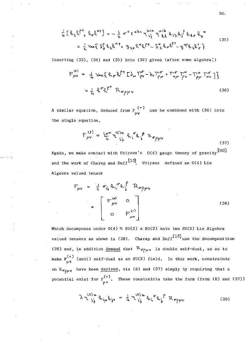
Inserting (33), (34) and (35) into (32) gives (after some algebra:)
A similar equation, deduced from F (-) can be combined with (36) into ~'J
the single equation,
(37)
Again, we make contact with Utiyama's 0(4) gauge theory of gravity[BO]
and the work of Charap and Duff[!~. Utiyama defined an 0(4) Lie
Algebra valued tensor
(38) ::::
Which decomposes under 0(4) ~ SU(2) x.SU(2) into two SU(2) Lie Algebra
valued tensors as shown in (38). Charap and Dufffl5]use the decomposition
(38) and, ~n addition demand that 12-D"('p\l is double self-dual, so as to
make F(+) (anti) self-dual as an SU(2) field. In this work, constraints v·~
on R~f~v have been derived, via (8) and (37) simply by requiring that a
potential exist for F(+). These constraints take the form (from (8) and (37)) }"\l
(39)
51.
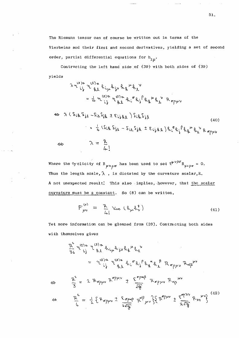
The Riemann tensor can of course be written out in terms of the
Vierbeins and their first and second derivatives, yielding a set of second
order, partial differential equations for h .. l.Jl
Contracting the left hand side of (39) with both sides of (39)
yields
(40)
"t~··o \~lS"o Po Mo \1 - "~~9.. I ~ VI.~ "h.~ ""'1. \t 6"fJJ-'V
Where the cyclicity of R has been used to set 'C.y.-vp6 R = 0. )" V f CS' p.:v p a-
Thus the length scale, A , is dictated by the curvature scalar,R.
A not unexpected result! This also implies, .l)owever, that the scalar
curvature must be a constant. So (8) can be written.
(41)
Yet more information can be gleaned from (39). Contracting both sides
with themselves gives
{ t '¥-cs-ffY -t <=Lapo~~ ~~

This is indeed a strongrestriction on the Riemann tensor for the
manifold, and it all follows from (8) and the assumption that a
potential exists:
Note that, if R = 0, (8) tells us nothing, since (40) shows
that ~ must vanish. Thus if we try and use (8) to construct a.
SU{2) field over a manifold with vanishing curvature scalar, (8)
merely gives us F y.v = 0, If R = 0, (26) must be used as a starting
point, and this is the approach of Charap,andDuff[151.
The Riemann tensor can be decomposed into R, R~v and the Weyl
" tensor, C , in the usual way, Pt>-V
'Rpa-/"v = Cll:>"Y." -+ ~ l c:a-f.l-" Ra-v + ~a-v Rr,v.-<}pv Rcrf'""-'h-P14rv)
52.
~ (43) -6 \.c.a-pJ-J''1Jov- ~pv~o-y)
where Cr~~~ enjoys the same symmetries as Rptr~v but, in addition,
contains no vestige of the Ricci tensor i.e.,
= 0
Using (43), (42) becomes
'R'l.-4R -p._Mv >""
. (44)
::: l C yv). f :t { t:2f_..-)- ( )-AV ~ y )( C )1-"VAr ± { t ?\folf' C )JV o\r J • ( 45)
~
There is onemore quadratic invariant in R which has not yet been }/''»fO"
used, and that is [491
We can derive an equation involving this quantity from(39~~nd the
duality properties of F(+) • Writing (39) as )/'\l
(46)
(47)
(anti) self-duality implies
Now,
~
Fl±) yv
=
=
contracting both
Ft.;!:) <..:ny.v 9 yv . 'F '::::' "R'4
~~ 1 '[ p <rol('
:::
4-3 b4- ~
53.
(48)
. [49] FollowJ.ng Lanczos (but beware of the fact,or of i missing in equation
(2.4) of that reference) define the following five quadratic invariants
cl,r I I = Ro~~ K
'l.. I'l.. ::: 'R
\Z' - .l t y.vpo-2..
~
\<C)_ J. t_>-'vpo
- 4. ~
(50)
(51)
(52)
R ol(3 )""V R p 0"' ~ \->
(53)
't. ~~ \: (1.
Ryv""~ R f6'_"t~ ~ (54)

Then (42) and (49) can be written
i I 9...= ~<'l + v..,
respectively. Subtracting (55) from (56) gives
1"3= K2..
Now the relation between the five quadratic invariants derived by
[49] Lanczos in (equation (5.5) of that reference) is
which is true for any manifold which admits a Riemannian metric.
Equation (57) is equivalentbwthe statement that the Riemann tensor
is double-self-dual. Inserting (57) into (58) yields,
I?..- 4-I,"" o
54.
(55)
(56)
(57)
(58)
(59)
which, in terms of the Ricci tensor and curvature scalar,,(51) and (50),
is
(60)
Equation (60), for a positive definite metric is true if andonly if the
f541 metric is Einstein (Petrov ). This can be seen most easily by
writing (60) as
(61)
Equation (61) must be satisfied at each point of space-time. At
any point, we can choose the metric to be diagonal (though, of course,
this cannot be done globally.) and, since the signature of the metric

55,
is (++++), each term in the sum on the left hand side of (61) is a
perfect square with positive sign, therefore each term must vanish
individually. Thus
(62)
Equation (62) and the constraint that R is constant,(40),are the
defining conditions for an Einstein metric. Not all manifolds admit
. [54] an Einstein metric, but those that do are called Einste1n spaces •
With (62), equation (45) gives a condition on the Weyl tensor
The san.ereasoning that was applied to (61) tells us that, for positive
definite metrics, with R ~ 0,
(64)
The upper (lower) sign applies for instantons (anti-instantons) constructed
using (8). Thus, if R F 0, we have
For a self-dual field to exist, the Weyl tensor must be anti-
self-dual
For an anti-self-dual field to exist the Weyl tensor must be
self-dual
Thus for R t O, the only manifolds that will admit both instantons and
anti-instantons via equation.· (8) are conformally flat spaces.
For R = 0, equation (8) cannot be used, but one can use (31) and (38)
. [15] as a starting point as 1n reference · •
The topological charge of the field (8) can be expressed in terms
of the topological invariants of the manifold, the Euler Characteristic)(,

and the Hirze. bruch signature it, which, for a compact manifold
[26) without boundary are given by ,
')( = \')..8 1"1"').
56.
(65)
(66)
Using (43) and (60), these can be re-expressed, for an Einstein space,
as
(67)
(68)
Together with (64), these give
(69)
Thus the topological charge'is, from (9), (40) and (69)
(70)
where the upper (lower) sign is for instantons (anti-instantons).
For R = 0 this result can still be obtained, using (38) and (6), without
assuming (8). [32)
The results of this chapter so far can be summarised as follows.
Starting from equation (8) (or its anti-self-dual counterpart) for
a manifold with R t 0, a self-dual (anti-self-dual) potential exists
only if the metric, g~v' satisfies the following conditions;
a) The metric is Einstein
b) The Weyl tensor is (anti) self-dual

57.
The topological charge of the configuration is given by equation (70)
Note that condition (a) implies that, since T vanishes for an (anti) !""~~
self-dual field configuration. Einstein's equations with a cosmological
constant (2) must be satisfied for a potential to exist. Thus the very
existence of a. SU(2) potential implies that Einstein's equations are
satisfied. This is in contrast to the R = 0 case, where consistency
with Einstein's equations is an extra condition which must be put
[151 separately (Charap and Duff ).
The above analysis can be formulated quite neatly in terms of
t . b . t d . t . . t . [36] d t k. th qua ern~ons, y ~n ro uc~ng a qua ern~on~c me r~c , an a ~ng e
real part of the metric to be g and the pure quaternionic part to be }'-\7
an SU(2) F, • This is reminiscent of Einstein's work on a generalised ~\t
theory of gravitation, where he considered a complex metric and took
the real part to be g'r"" and the purely imaginary, part to be a
. (29 39] U(i), electroma·gnet~c F ' . We construct the quaternionic metric.> v-v as follows, Given a metric which satisfies both a) and b) above,
choose Vierf?eins, ~· l<Mi~'>o) for the metric, which can be considered t }" '
as four quaternions h = e. h. • Them construct the qua tern ionic metric }1 ~ ~Jl
(71)
and take
(72)
where the factor R is necessary on purely dimensional grounds. Then;
F. ~ is automatically self-dual in the metric g~v· Assuming that a )<'-. r
SU(2) potential, Ap' exists for F\J'~ gives
(73)

Using the cyclicity property of the Riemann tensor
(73) can be written as
\'1.
R
Then, using (72), equation (36) and condition a) can be written as
The potential for F is given by (26) )J''\J
From the definition of the Weyl tensor (43), we see that (76) gives
which, together with cP }-'; pv = 0, can be written
::: 0.
Equation (80) is the quaternionic form of condition b).
In general, the task of classifying all four dimensional Einstein
[54 431 spaces is a fascinating, but unsolved, problem ' • Some known
58.
(74)
(75)
(76)
(77)
(78)
(79)
(80)
Of [7, 43, 54) 84, 82 X 82, 4 II"" 2-u. -p2 K3 tr Pt. examples such spaces are , T , """P ,. <r , , \1....
4 4 [5 7J . Of these spaces S and T are conformally flat ' and so (64) 1s
automatically satisfied: Thus both instantons and anti-instantons exist
over though all Einstein metrics on T4
are flat, as can be seen

59.
from equation (67) and the fact that~= 0 for T4 [ 7? 81 x 8 3 is
also conformally flat, but it is known not to admit an Einstein
. [43] 2 . metr~c • <C P adm~ ts an Einstein metric with non zero R and its
Weyl tensor is either self-dual or anti-self-dual, depending on the
f51 orientation of the metric • Thus either instantons or anti-instantons
2 -2 may be constructed, but not both. ~P =II< a:P admits an Einstein metric
r531 with non-zero R but the Weyl tensor is neither self-dualnor anti-
self-dual and so it will not admit an instanton structure via equation (8).
82
x s2 has an Einstein metric with non-vanishing scalar curvature.
Its Weyl tensor does. not satisfy equation (64), but the manifold has
other interesting properties which make it worthy of further study,
and it will be considered in chapter six. K3 , Kummer's surface,has
vanishing Ricci tensor and so is Einstein with vanishing scalar
curvature. It has (anti) self-dual (depending on the orientation
chosen) [51
Riemann and Weyl tensors, . A metric for K3
has not been
explicitly constructed, though implicit and approximate constructions
. [33 48] have been g~ven ' .
Ths spaces s2 x 8
2, K
3 and <CP
2 are of spacial interest since
. [401 they constitute the space-time "foam" of Hawk~ng • In that
reference it is conjectured that, since the gravitational action
contains a dimensionful constant, large fluctuations in the topology
of space--time will produce only small changes in the gravitational
action, provided the fluctuations occur over distances small compared
to the natural length of the action, the Planck length,
(81)
and thus would be expected to give important contributions to the
gravitational action in any functional integral approach to quantum
gravity. [501
These ideas are closely allied to those of Wheeler .
60.
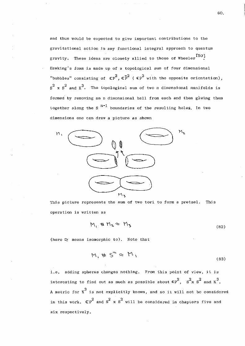
Hawking's foam is made up of a topological sum of four dimensional
"bubbles" consisting of <CP2
, <rP2 ( <I:P
2 with the opposite orientation),
2 2 3 8 x 8 and K . The topological sum of two n dimensional manifolds is
formed by removing an n dimensional ball from each and then gluing them
n-1 together along the 8 boundaries of the resulting holes. In two
dimensions one can draw a picture as shown
n,
s~® e 8'6
M? This picture represents the sum of two tori to form a pretzel. This
operation is written as
(here~ means isomorphic to). Note that
(82)
(83)
i.e. adding spheres changes nothing. From this point of view, it is
2 interesting to find out as much as possible about ~P ,
A metric for K3
is not explicitly known, and so it will not be considered
in this work. ~P2 and 82
x 82
will be considered in chapters five and
six respectively.

CHAPTER 5
SU(2) AND U(l) FlELDS IN~ p2
61.
In this chapter the formalism of chapter four will be applied to
~P2 , a four dimensional Einstein space with constant scalar curvature.
2 The question of SU(2) Yang-Mills over~P has also been considered by
Atiyah [51 [321
et al and Gibbons and Pope • n In chapter two, (.P models
were considered in which the fields were <CPn valued, and the 'space-time
was a two dimensional sphere. In this chapter the space-time is four
2 dimensional ~P and the fields will be SU(2) (or U(l)) Yang-Mills fields.
2 Considerations of the geometry of ~P are greatly simplified by the use
of complex co-ordinates and, for this reason, a brief diversion will be
made to explain the concept of a complex, Kahler manifold (of which tP2
) f3 ' 64] is an example
Locally, a n-dimensional, complex manifold is a 2n-dimensional,
real manifold, parameterised by n complex co-ordinates. Let ~~S
p = \, ••.• ~"' be real co-ordinates and ~;z.o<) )o< = 1, ... ,n be complex
co-ordinates. Then a real line element on the manifold is given by
2 For ds to be real, the complex metric must satisfy
If it is possible to find a complex co-ordinate system for which
'}o(~=<i~r; = o , then (2) implies that~<>~'(} is Hermitian, as ann x n
(1)
(2)
complex matrix. In this case the manifold itself is said to be Hermitian.
:l. c:CP is such a ma"l\ifold. In a Hermitian co-ordinate system (1) reduces
to
(3)
62.
where we have adopted the notation 2~ =- -z.~ One can think of ~ z"\ z. ';!}
as 2n complex co-ordinates for a larger space and z~ = z.~ is then a
condition which restricts us to lie in a; n dimensional complex subspace.
Contravariant and covariant tensors can be defined on a Hermitian
manifold in the usual manner, and indices raised and lowered using
~~F . Note that barred indices become unbarred upon raising or lowering
and ViCe Versa I SinCe <a'ol? ::: co~r. : 0 • Now let us define the 2-form
This is real, since~~~ is Hermitian. If it so happens that the
exterior derivative of K vanishes (i.e. K is a closed 2-form)
-J... \<. = - ;.(. '6}1' '11 ~~ - 'dO( ~y~ J d..-z.~" J.-. :z.c(" J-. '2 ~
-"I. l d) ~ol~ - d(i ~ ""~) J..-1 )'. <k :z.« )'.. d- -z{6
then the manifold is called a Kahler manifold and K is called the
(4)
(5)
Kahler or fundamental 2-form. Condition (5) is equivalent to saying
that the curl of the metric vanishes
'D~ ~o\~ - )"" ~¥0 = 0
) ~ ~ <>1.0 - )fi ~ tl. y ~ 0
(6)
and so the metric can be derived from a potential
(7)
1£ is called the Kahler potential. C P2
is a Kahler manifold.
As a consequence of (7), the usual expressions for the Christoffel
symbols and Riemann tensor simplify to,
(8)

63.
all other components vanish, due to (6). In particular, the cyclicity
of the Riemann tensor is expressed as
since 'il-o~~1~ vanishes.
The Ricci tensor also simplifies nicely, using the identity
one finds
2 This elegant machinery can now be applied to ~P .
The general construction for <CPn was given in chapter two,
~P2 can be considered as the space obtained by identifying all the
points of ~3 which differ only by a scalar multiple
Where c is a complex scalar. Hence the name, "projective space".
(9)
(10)
(ll)
(12)
The points of ~P2 away from Z 0 = O, can be parameterised by two complex
variables of any magnitude
(13)
~ 4. The points (u
1, u2 ) also parameterise <I: ~ ~ The remaining points,
~ c:t: ~ z 0 = 0, are those which are obtained by identifying points in <I: c::
which differ only by a scalar multiple
(14)
I ~ 2 These points constitute the mai'lifold <C P ~ 5 • Thus <Cp can be thought
4 2 of as :IR , compactified by adding a S at infinity (in the same way
as s4 can be thought of as '\B. 4 compa,ctified by adding a single point
at infinity.) <C P2
has been proposed as a gravitational instanton t32 ' 25]

64.
because it can be given a metric which satisfies Einstein's equations,
CRr-"""'A~Mv,h a constant) and it has finite gravitational action.
[51 f32l 2 References and also consider SU(2) Yang-Mills over ~P .
• < • • • • [261 The metr1c 1s the Fub1n1-Sudy metr1c ,
(15)
(the scale has been set to unity.) In the form (15), g~~ is manifestly
a Kahler metric, with Kahler potential
(16)
2 1-1 2-2 1 2 where \~\ = u u +u.u. Let u = Y~. u = Z, then (15) is
(17)
where ~ labels the rows and ~ the columns. The inverse of (17) is
~d. ['"~~ ~·j li+\C~.-1').) - - (bcii ~ ==- -:::: iJ
"2.~ \+ '2.'=i.
(18)
Now we can use equations (18) to find the Christoffel symbols
T'~ ').:~ '2. 1,2. l''Z.'Z. :::-:::: l\ + I 'X-\ 'l.) ~'-tr l\ + \':Y-1 2. )
-r't ::- T'~ .z T'oz. T' 'Z. :::- ~ 'i:Z. 2";f : - '1..,.. 'Z.~
l.l -to \')(..\ 'l. ) {.l+lll<-\'4)
(19)
\~ 'Z.
:. 0 l' 'i'i ;:- 0 'Z.'l.
and their Hermitian conjugates. All others vanish.
For the Riemanntensor,
\1-- '-3 ~ 'i '?! =: ~U+-z.7.)l 'R. 'Z."i. 'Z:Z. :::
~ \ l+'i~ )'l. (\+ \~\,_ )lr l\+l'.l<.\2.)4
\2.~~'i'i: -:. ')..U+--z.7.)~'Z. Rz.:zz.~ "" ~U+~~)"ai
l.\ + \?L\2.)4 l\+ \?<..\2.) It- (20)
R ~~'Z.'1! = ')_l\+ z'i. )'1i R-z.i.~;. ::: ')..U+ 'i- '11) 1:\ z
l\+ \')(.\1. )LI- l..\+ \~1'-)4

(_I+~ V:l)l\ + ~z.) + '1J~%. :Z.
(..\+ \~\'!.)!&.
'l..ll~ zi ):z.~
(.\+ 1~11-)4-
:::- ?.. \.HL6~)~:Z
u ~ \Jl.\2. )4-
- ?..'q"'z'J..
(_I+ 1?.-\1-) 1.!-
\_l+z'i )l';~~) +'3~'2.:Z.
0 t- \?'-\ 2.. ) '+
~ ll+ 'A-~ Yra 2.
U+ IJl.l'l.. )'-'
~ ~~'3:1..
(_\+ \'J~\~ )4
?...,(.\+z:Z.)'?Ji
l\+ l:ll-1~) 4
other components either can be found from the symmetries of the
65.
(20) contd.
Riemann tensor (8), or they vanish. Note the interesting factorisation
(21)
(the ordering of the indices in (21) is crucial). This factorisation
is not a general property of Kahler manifolds, but its form simplifies
2 the calculations for ~P •
The Ricci tensor is, from (21),
showing that (17) is indeed an Einstein metric, with cosmological
(22)
constant,J\= 3. (22) could also have been obtained directly from (11),
2 -3 since det ~~r~ (1+1xl ) • From (22) the curvature scalar is
(23)
In the 1.ight of (23), note the similarity ( and also the difference!)
between (21) and the Riemann tensor for s4 ,
(24)
The Weyl tensor is defined by equation (4,43), in any co-ordinate
system, and so in our complex co-ordinates we find, using (22)

and (23)
Co<~YS-===- '}o~~~~~
C<><Y ~ ~ = ~ ct~ <}y~ - '1-oqi oa- ¥S
)" - c~ -Note that C "'-'~~'"~ i o\~~ = 0, as it should be.
To examine the duality properties of (25), define four real
2 co-ordinates ~ •:JJ''L }l = 0, ... , 3, for <C P via
~~ ry,., 0 - ;. ')(.. 1 -::J..-0= i(.~+"i)
I ":}.-) ':: i.\"1-"11) ). _.;,-:x,. 'Z. ':: 'J... ?..
).
"Y-. "' l cz.;-'2. ') 'l..
I i (_'2.- 2) ')C..:' :I.
66.
(25)
(26)
Tensors can be transformed between real and complex co-ordinates using
d')<..o d')(.O J?!- a ":ll-:1. 1 -::::. - ,. - = ...
~~ il~ d2. '.\::Z. '.l...
~'):."4 )~1 ):x. I )::x, I - = -= :: - - = ~I ~'?! 'A~ )-z. ';)'i ')..
For example, the Weyl tensor transforms as
- - ),.__lA a-:x."' )?1..~ a')...<$'
co{ f)'~ - );;."'. ) "'~ . i>u.."Y • d 1). ~ c. J"" p 15"
C -- - ?J-:? a-x.v ~ >-r a-:>'-cr o(~r'S- ~0\· ~v-y'"dv.~·a\A.s c.,.....,p~>".
Hence the (anti) self-duality equations for the Weyl tensor in real
co-ordinates
== + I -~
(27)
(28)
(29)
( ~~ ~~ become, in complex co-ordinates note that, since ~ - ~ ~ -o p.v - o o(~ 'h."' (lJ~-" '
~'Z. .t C~7.o<(i :z~ Cz~c:~.~ c o(,~ ::: c ol~ ::: -r ~ '1'-r~ ~~¥~
c "1-'2. - c. '1%. <:>), (3 t;)i: c:. ~7.0(~ = c --o\~ ;.. ':::: + ~~'(~
0(0 hl~r~ (30)
c ~'a - ::: + C.-z. 'i.e>\~
~~ cW:. ~y~
Where ot ,(1"' l,'l. With (25) and (17), the lower signs hold in (30).
Thus, in these co-ordinates, the Weyl tensor is anti-self-dual and
we will proceed to construct a.·self-dual Yang-Mills field in <tP2
,
using the methods of chapter 4. First look for Vierbeins for the
metric (17)
67;
(31)
By inspection, h has the form
(I+I'X-1~) (32)
-then (31)' gives (17). Here, and henceforth, a,b, ••. , a,!;>, ... label
locally flat complex co-ordinates, i,j, ••. will label locally flat
real co-ordinates, 0( 1r 1 ... 10j )~ 1... label curvilinear complex co-ordinates
and Jl ,IJ, . . . label curvilinear real co-ordir.a tes.
From (4.8), a self-dual SU(2) Yang-Mills field is given by
(33)
..... '\).. wl}ere "R = 12," = ~t have been used. The recipe for constructing
h is given in chapter four. Converting (33) into complex co-ordinates J.l '
requires some care, however. From (27) and (33)
r~._ = -h.~ FQ'l.- \=~ 1 +l.l l=o, + F;'l. )~::: 1 1~:, \. \. ~ 0-ti.~_, )\.. ~: +\.~'\) -l~.,. ;.\.~, )l~~ +1. ~~)~
F~:z: = -h.~ro .. - f"),-1.lro,+r~~)~ = 1'6
~\..~o..:\. .. ~~')\.~~-'-~n-l~'l.-~~.)l~!-1.~\)}
F~-z..., -h.~r" .. + r,1 + i\.Fo,-1-,,._)~-= TI, ~\..~o-'-~~J{~+'-~i)- l~·t:t\.~,)\:~~-~~~ )t \=" ~:Z. = ~ £:_ FQ'l. t- F,, -\, l\=o, -1--.,'1.. )\ = f~:. ~ \.. ~ 0 +\.~-., )l ~~-i-t;)- l ~'1.-i.~, )l t_~ +·~.~; )~
~ 11q ~ t \, F,o -::: \\ ~ \. ~c,-t'-~~ )\.~~ -\.~~) -l~o- \.~1 )l~~ T'-~~ I}
F-z.i.::: ~\. f 1'l.::: J.. ~\.~~+"-9-,)lt~-\.~i)-\.~'1..-;,t,)l~!+;,~t)'\ \(,
(34)
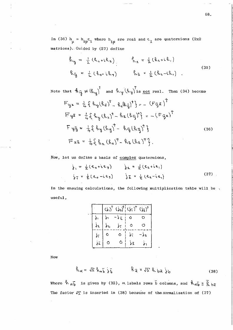
68.
In (34) h ~h. ~- where h. are real and~- are quaternions (2x2 }.l l.Jl l. l.Jl l.
matrices) .. Guided by (27) define
(35)
t I Note that oft~ ~ lt~ j and "h'f \~'a') is not real. Then (34) become
F~'Z. = "4 t t.~(tz:)t' _ ~'1:(~'1)t~ =- _ (F~z )t t
F ~2 ::- i;, ~ {. '0' (. ~ .. ') t - ~ ~ l t 'i \t 1 ::- - l F ~ 2.)
F' ~~-= -it~~~ l~~ lt- lh'a l~~ lt ~ (36)
\- ,:z. '"' ~~ ~'2. C~z.)"- ~2-l~i 1-r1.
:Now, let us define a basis of complex quaternions,
. I l . ) ~~ "' '[. ~() -t. Q..3
~~::: :t(~~~,+io..,)
-~i:: -t l.Q..~-t.~,) (37)
In the ensuing calculations, the following multiplication table will be ,
useful,
~~ -~- I C) 0 'l..l . . I h.. J.i I 0 0
------- -'----------1 •
0 C I ~~ -,h. I
0 0 l \ ii I <!',._ }\ I
Now
(38)
Where ~ c1. "£ is given by (32), 0\. labels rows b columns, and ~ol.b ::: ~ b~
The factor ~ is inserted in (38) because of thenormalisation of (37)

and
etc. With these definitions
~~-:: Ji' ~(\~1- :vz.:Z:) h + .'1 "Z. ~ ~~ ~ )''"'~'"') 1?-1
t_~::: 6 ~ L\'X-I-\-1-z..z)},- i..:Z.~ ~~JAI+I'J<.I:l..))-x.l
~-z. = ~ ~ i.z 'a h + <yx.l- '-'a~)}~~ A'"~-'~''") ,:x.l
~:=i. = ~ ~ -~ 2 ~ }, + ~yx.\+i ~~) ~ 9.. )/('''"'~''") I~ I
Using (40) and (36) one finds, for the self-dual field
F- "' 2.2.
F ~-z. = \="" ~ :z = o
I ~ 'l.~1,.Q..'3 [-z.i:\.'b~--z.:Z:) -I':JC.I'l.] -t ~ ~ll- '1Z \:z.Z:+il-:x..l) ~ (.\+ I?C\'l.) \?'\
-~ ~i-z.-ra<__z.i.-i.\~1),
\ ~ l t -\,~~ -z.-q, [zi:-~V.-+ !l.i,I"Xl] ~ \.1+-I?GI"-) 1~1 0
69.
(39)
(40)
(41)
_ ~~ll.[-z.Z."-A'~+IXI'l.+\ITI~'t~-zi)] + ~ ~i,Z.ll..~!l,.r
It is straightforward to check that F~0 given by (41) is self-dual
in the sense of equations (30). The calculation of a potential for
the field (41) proceeds via (4.26). The algebra is somewhat tedious,
but eventually one arrives at the following expressions,
As a check one can put (42) into
(43)
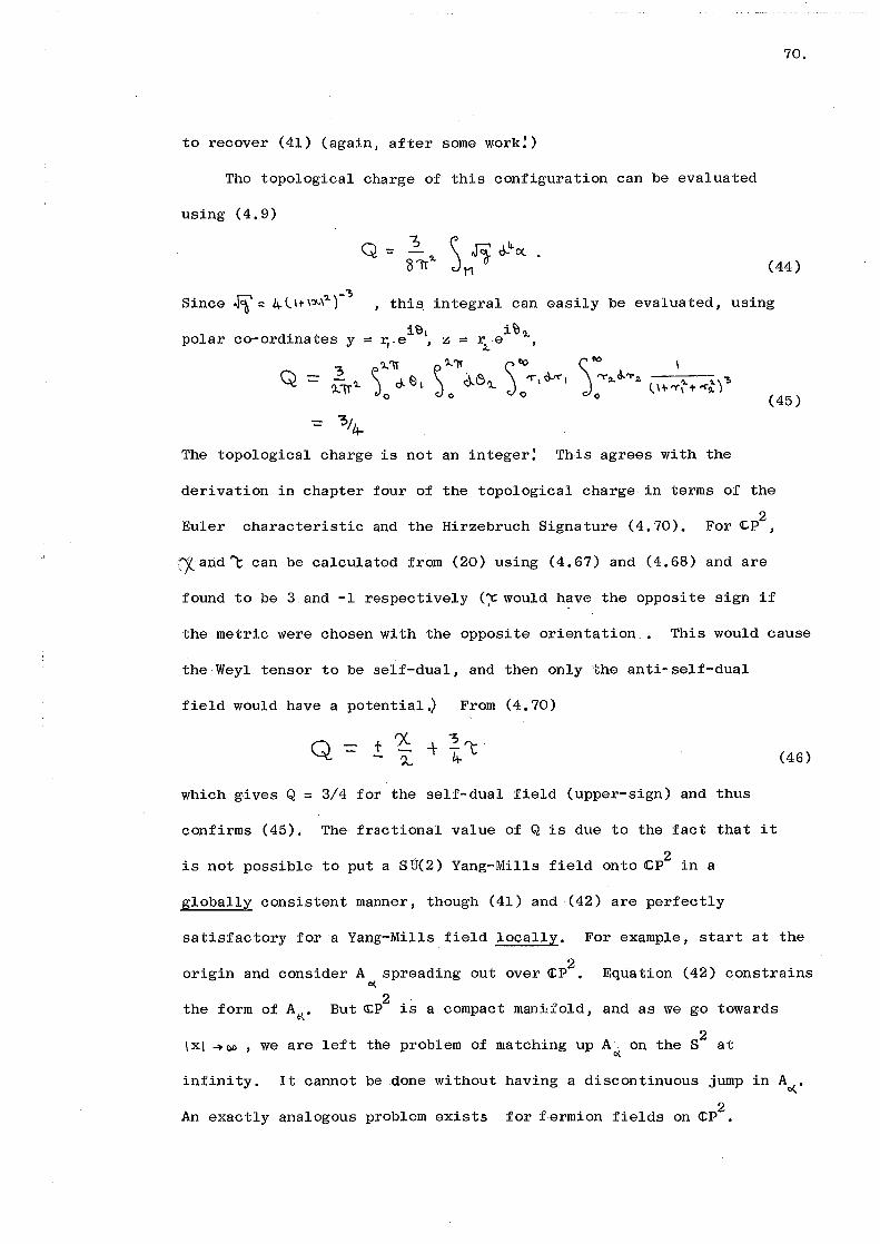
70.
to recover (41) (again, after some work!)
The topological charge of this configuration can be evaluated
using (4.9)
(44)
Since ~:: 4.(1+\'J\.\'l.r~ , this integral can easily be evaluated, using
ie, i~'>-polar co-ordinates y = r,"e , z = r,_.e ,
"3 \.?.."tr ~ ?.,1f \to Q = 'A.lT'l. Jo c~-e, Jo d..~'l.. Jo"T",d--r-,
(45)
The topological charge is not an integer! This agrees with the
derivation in chapter four of the topological charge in terms of the
Euler characteristic and the Hirzebruch Signature (4.70), 2
For CP ,
,1-and "'t can be calculated from (20) using (4.67) and (4,68) and are
found to be 3 and -l respectively (~would have the opposite sign if
the metric were chosen with the opposite orientation.. This would cause
the·Weyl tensor to be self-dual, and then only the anti-self-dual
field would have a potential.) From (4,70)
(46)
which gives Q = 3/4 for the self-dual field (upper-sign) and thus
confirms (45). The fractional value of Q is due to the fact that it
2 is not possible to put a S{T(2) Yang-Mills field onto CP in a
globally consistent manner, though (41) and (42) are perfectly
satisfactory for a Yang-Mills field locally. For example, start at the
origin and consider A spreading out over ~P2 • Equation (42) constrains c(
2 the form of A<J... But <I:P is a compact mani,fold, and as we go towards
\XI _,.()I) , we are left the problem of matching up Ar:J.. on the s2 at
infinity. It cannot be done without having a discontinuous jump in Ac('
An exactly analogous problem exists for fermion fields on <r:P2
•
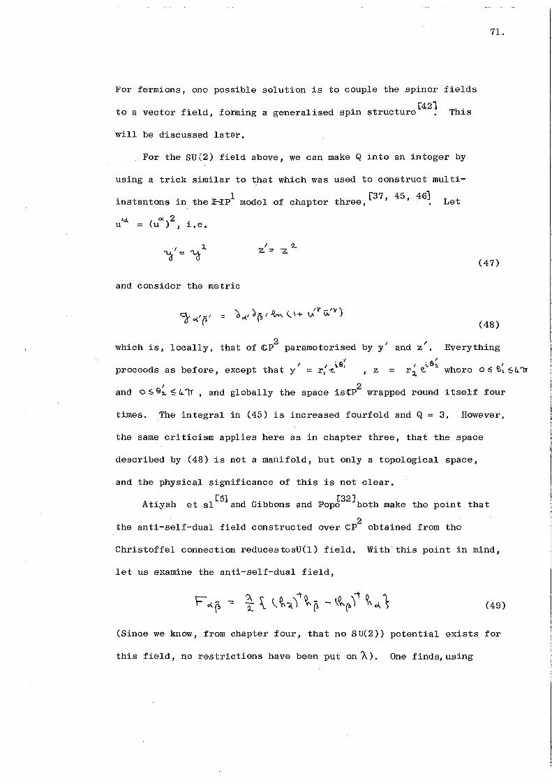
71.
For fermions, one possible solution is to couple the spinor fields
. . [421 to a vector field, forming a general1sed sp1n structure • This
will be discussed later.
For the SU(2) field above, we can make Q into an integer by
using a trick similar to that which was used to construct multi-
1 h [37 1 45 1 46] instantons in the .IH:P model of chapter t ree, Let
u'"" = (u0() 2 , i.e.
I !l... z ::.- "Z.
(47)
and consider the metric
(48)
which is, locally, that of cP2
parameterised by y' and z 1• Everything
I 1 ~Q~ proceeds as before, except that y = r,~ I "\9~
1 Z = r:l, e_ Where 0 ~ell ~4_1f
and o ~ e~ ~ 4.11' , and globally the space is~P2 wrapped round itself four
times. The integral in (45) is increased fourfold and Q = 3. However,
the same criticism applies here as in chapter three, that the space
described by (48) is not a manifold, but only a topological space,
and the physical significance of this is not clear.
[51 [32] et al and Gibbons and Pope both make the point that
2 the anti-self-dual field constructed over <r:P obtained from the
Christoffel connection reducestoaU(l) field. With this point in mind,
let us examine the anti-self-dual field,
(49)
(Since we lrnow, from chapter four, that no SU(2)) potential exists for
this field, no restrictions have been put on A). One finds, using
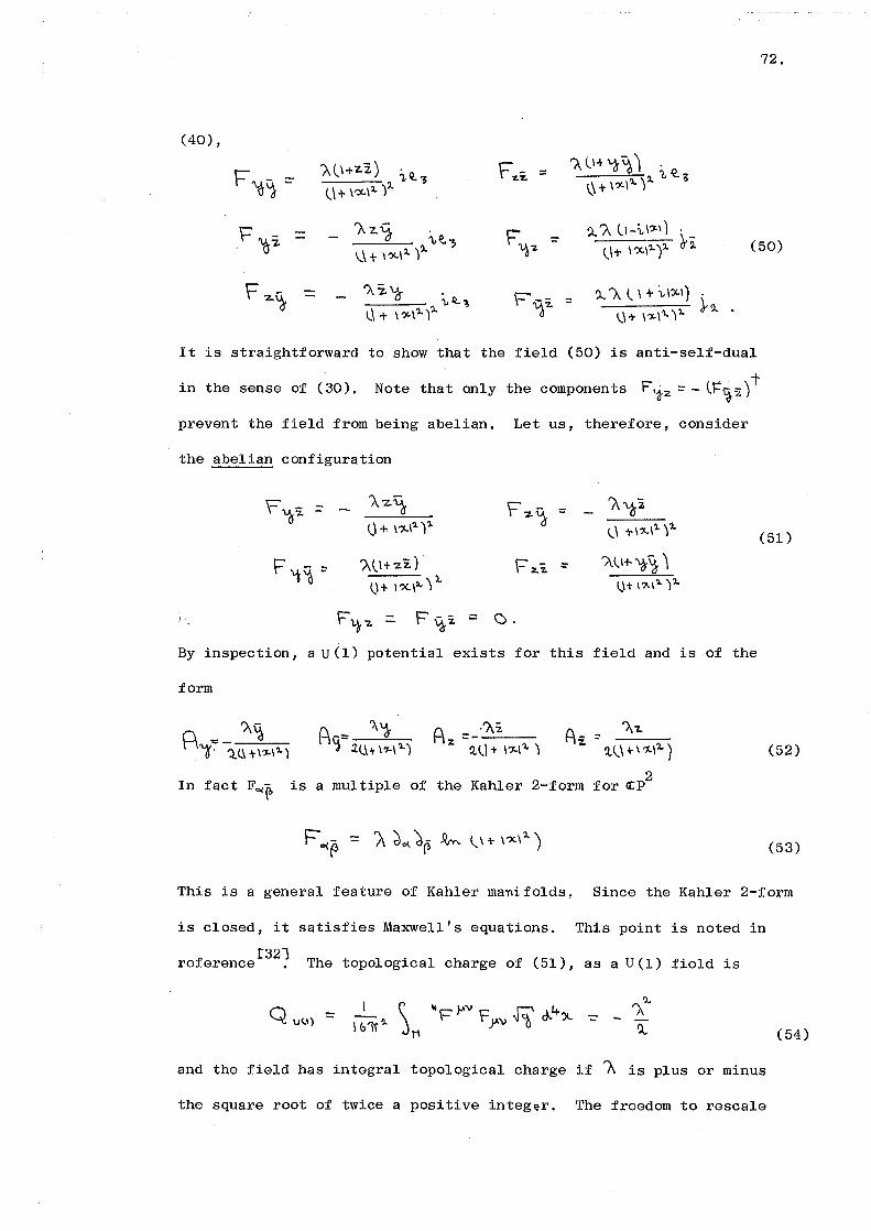
72.
(40)'
F~i 'Ali+ZZ) i~ f""oz.i. = ?..{.1+'1J~l .
= l. 1. .(?_; ?.. ~ \j + \?<.\?..) l\+ \'X.\l.)
~'A ll-i.1~ 1 ) F~~ 'Az.~ .
F'i-z: d-i 'V~; = \..\t\':X.\:1.):). (.\1" \'X-1'-'? (50)
~ ~~ ').. :z. 'a- . F"1,:z.
?.,. A. ( \ + ;, \';I:. I) }').. -u.Q..; ::
\..\ + \ ?<-\'-):). \,\+ \':X-\'1,. )'l.
It is straightforward to show that the field (50) is anti-self-dual
in the sense of (30). Note that only the components F'iz ::- -ll=·~zJt
prevent the field from being abelian. Let us, therefore, consider
the abelian configuration
F~:z. = '\-z.~ ~"2.~ = 'A~z (_\ + \':X.I'J.)'l. \..,\ ·H?C.I'l.)'l.
(51)
F '1~ = 'All+z"£) r- :z.i =- 1\U-r~~ I \1+ \?C..\:1. '\ l.. l.\-t\?1.\').)l.
By inspection, a U(l) potential exists for this field and is of the
form
A ...: c'Ai z -----
~U+ l?\.1,_) (52)
In fact F~~ is a multiple of the Kahler 2-form for ~P2
This is a general feature of Kahler mani.folds, Since the Kahler 2-form
is closed, it satisfies Maxwell's equations. This point is noted in
[321 reference • The topological charge of (51), as a U(l) field is
(54)
and the field has integral topological charge if A is plus or minus
the square root of twice a positive integ~r. The freedom to rescale

73.
by an arbitrary real factor is not present in the SU(2) case -- '
due to the non-linear nature ofF~~ , equation (43). The U(l)
bundle, with gauge field (53), over~P2 is in fact topologically s5 •
It is the Hopf fibration Of 8 5 [32' 57].
[421 It has been noted, by Hawking and Pope , that a U(l) field
on ~P2 can cure the problem of putting spinor fields on ~2
mentioned earlier. To see how this can happen, we need the index
theorem for the Dirac operator on a compact manifold, without boundary,
0 [26l in the presence of a U(l) gauge f1eld . With no gauge fields
present, the index theorem tells us that the number of positive
helici ty solutions ()\) of the Dirac equation minus the number of
negative helicity solutions (~_) is related to the curvature of the
manifold by
; ~41r"' 5 t1 ~ ~\Jo1(3 R P"o.i" ~ cl.. 4- :x. (55)
=-"'t:f'8.
For a:P2
, with the chosen orientation, 1:: = -1 and so the reight hand
side of (55) is not an integer. This is a reflection of the fact
that spinor fields cannot be defined on ~P2 and may be taken as a
proof of that statement. In the presence of a U(l) or SU(2) gauge
field, however, (55) is modified to
respectively (the generators of EU(2) are normalised so that T.,. <.~i.lt)):::-!1..~;.~ •
For the self- dual SU(2) field derived earlier ( 41), Q.,ut~l -= ~~'+
and (57) becomes
(58)

74.
Thus, putting ~ 8U(2) field on the manifold enables spinors to
be defined on ~P2 in a consistent fashion: However, we are still
left with the problem of non-integral Q i.e. the gauge field does
not match up.
For a U(l) field, (56) becomes, with (54)
(59)
so that a judicious choice of A will lead to a consistent definition
of spinor fields e.g. 1\ = 3/2 will do.
It is also possible to make")).._- 'V..; in (55) an integer without
introducing gauge fields at all, using the method mentioned previously
(47), (48), e.g. taking y1 = y4
, z' = z4
increases all integrals over
the space by a factor of sixteen, making~+-~- an integer.
Again,.however, we are no longer dealing with a manifold.
In this chapter, the methods of chapter four have been applied
to <CP2
, a four dimensional, compact, Einstein space, with non-.zero
scalar curvature. With the orientation on 2
<C P chosen so that the
Weyl tensor is anti-self-dual, SU(2) Yang-Mills fields have been
explicitly constructed, with topological charge 3/4, indicating a
global obstruction to the field. The anti-self-dual field reduces to
' a U(D field, and it has been demonstrated how this can cure the problem
f . . 2 o putt~ng sp~nors on CCP •
In the next chapter, the analysis of chapter four will be applied
2 2 to another Einstein space with non-zero scalar curvature, S x 8 •
The Weyl tensor for 82
x 82
is neither self-dual nor anti-self-dual,
2 2 however 8 x S is a Kahler manifold and as such is worth studying
from the point of view of U(l) fields.

75,
CHAPTER SIX
U(l) INSTANTONS IN s2x s2
In this chapter, U(l) instantons over s2x s2
will be constructed.
s2x s2
is a compact, Einstein manifold with non-zero scalar curvature.
The Weyl tensor is neither self-dual nor anti-self-dual and so SU(2)
fields will not be considered. However, a Kahler metric exists for
s2x s2
and so the Kahler 2-form gives a non-trivial Maxwell field,
as pointed out in the last chapter,
2 2 To construct an Einstein metric on S x S , we simply take the direct
2 2 sum of two S metrics, The invariant line element on S is
where o~El~'l'r, o~<l>..,'l.1r (the radius of the sphere is set to unity.)
2 2 On S x S we take the line element to be
That this
is a Kahler metric can be seen by parameterising each s2 by a complex
co-ordinate
Then (2) becomes
(l)
(2)
(3)
(4)
In the form of equation (4), the metric is manifestly Kahler, since it
is derivable from the Kahler potential
(5)
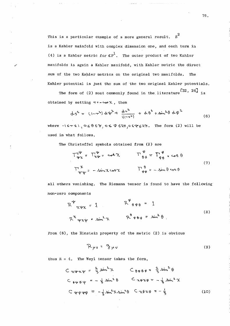
76.
This is a particular example of a more general result. s2
is a Kahler mainfold with complex dimension one, and each term in
(4) is a Kahler metric for ~P1 • The outer product of two Kahler
man~folds is again a Kahler manifold, with Kahler metric the direct
sum of the two Kahler metrics on the original two manifolds. The
Kahler potential is just the sum of the two original Kahler potentials.
Th f f ( 2 ) f . h 1 . t t r32, 26] . e orm o most commonly . ound 1n t e 1 era ure 1s
obtained by setting '"('=-~'X., then
(6)
used in what follows.
The Christoffel symbols obtained from (2) are
T'~ ir c::..c-*. 'X l'q; T'<P :: "j1'X. '\jr :: = "" c..c-t e
'I\!" "X. f)¢ <Qe (7)
\''X. - ~'X.~'"Y..
T'~ :: -~8~19 V"'\T'::: ~<(>
all others vanishing. The Riemann tensor is found to have the following
non-zero components
""" 1
t 1 R ec:pe =-'R '"X.~ ::
')(. e ~'-e ~'>...'"'/... R <~>~~ ::
"R "\\''X. '\)r ::'
(8)
From (8), the Einstein property of the metric (2) is obvious
(9)
thus R = 4. The Weyl tensor takes the form,
c.. &"\>' e "\'"
(10)

77.
plus components obtained by symmetry operations, all others
vanishing. (Note that, as a consistency check cY'"\If'"P = 0). The
Weyl tensor (10) is neither self-dual nor anti-self-dual, and so the
method developed in chapter ~ will not yield a . SU(2) field.
However, the Kahler nature of the manifold makes it worthwhile to
study U(l) fields in the metric (2).
Consider the Vierbeins
If we try and construct a SU(2) field, as in (4.26), it reduces
to a U(l) field as follows.
Let
then one finds, using (11) and (7) that
{\ - c:.cO"'X.. l""'\'1~ - - -- Q..
'I" '),. I
which gives a self-dual field tensor,
~f.. --~~
'l..
:::: 0.
An anti-self-dual field may be obtained by changing the relative
sign of P.,_y-and \'=" &ql (or equivalently A"4>- and A <P ) • This can be
achieved by transferring the (t) in (12) from the second to the
first factor on the right hand side. An alternative method of
constructing an anti-self-dual field is to change the orientation
2 2 2 of one of the S factors of S x S • This amounts to changing the
relative sign of the terms in brackets in equation (2).
(11)
(12)
(13)
(14)
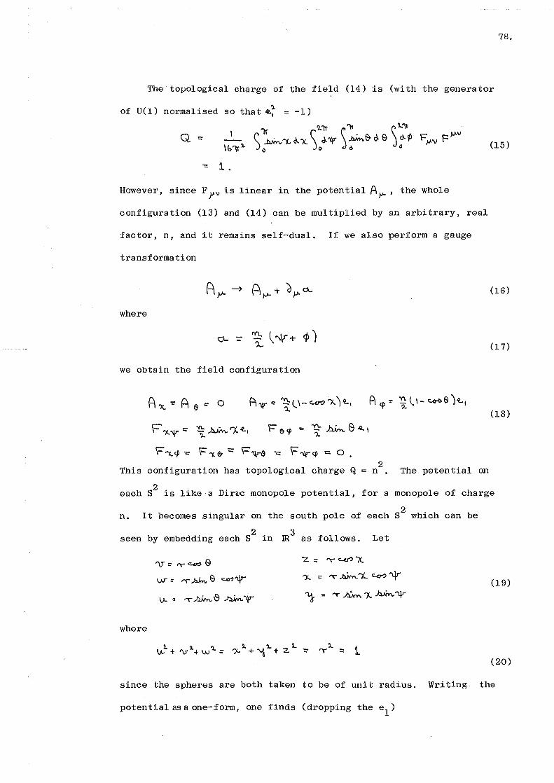
78.
The topological charge of the field (14) is (with the generator
of U(l) normalised so that ~~ = -1)
Q = 1r 'l."tr ~"' ~?...11' C' .AIM.~ d--x. C d. '111" ~&d-e o. P lb1T'l. )<> Jo 6 d
"": 1.
F ~J.-'V )Jo'\J ,-
However 1 since F J"" is linear in the potential A y- 1 the whole
configuration (13) and (14) can be multiplied by an arbitrary, real
factor, n, and it remains self-dual. If we also perform a gauge
transformation
where
we obtain the field configuration
A-x.;A \9 = 0 P\'l\" =-~(.\-~'X-)~, A <P,.. ~ (\- c.c-t>e)~, 'l.. 'l.
F"l<."'\""= "!: .AJM. 7.- ~I F &<P "" '!:~e~, 'l. ?..
\:="'.C/l':::' \=' "t-19- ":::." \='\lr\9 "::: \=' 'W""<P ~ 0.
This configuration has topological charge Q 2
The potential = n on
(15)
(16)
(1 7)
(18)
each 82
is like a Dir~c monopole potential, for a monopole of charge
n. It becomes singular on the south pole of each 82
which can be
seen by embedding each 8 2
in m? as follows. Let
'\}'" ::: rr <:.o'O e v.r= ,...,~e ~"\"'" (19)
V- = ,...,~~ him-"V
where
(20)
since the spheres are both taken to be of unit radius. Writing the
potential as a one-form, one finds (dropping the e1
)

79.
(21)
Which is singular at z = -1 ('X = 1r ) and u = -1 ( t:l = '1f), the south
poles of the two spheres. This is the familiar Dirnc string singularity,
except that, in this case, they are not strings, since the spheres are
of fixed radius, As is well known the singularity is illusory [62~
and can be avoided by splitting the~tential up into two parts on
each sphere
-= 1_ li\- c::.c?"X) J-.v + ~ l± '- c.Q?e) d-.~
A+ is well defined away from the south pole of both spheres and A is
well defined away from the north pole of both spheres. + Furthermore, A
is related to A (away from both north poles and both south poles)
by a gauge transformation
At the north pole of one sphere, but the south pole of the other, a
non-singular potential is defined by taking the upper sign in one term
+ and the lower sign in the other ':in (22),, which is again related to A- by
(22)
(23)
a gauge transformation. Thus four co-ordinate patches are needed in all
to define a non-singular potential.
If we think of~ as a compactified time co-ordinate and X as a
compactified radial co-ordinate (via .,- = ~i: ) , then (18) is like a
"dyon" in that F'X.\jr can be thought of as an electric monopole and F \9{)
as a magnetic monopole. For the field to be self-dual the electric
and magnetic monopoles must have the same charge, n, Then
is like the Dirac quantisation condition in four dimensions.

80.
We have now examined two compact Einstein manifolds with non-zero
scalar curvature, ~P2 and s2x s2. There is one other solution of
Einstein's equations with positive, non-zero, scalar curvature which
!l. -?.[53] is explicitly known, and that is the Page metric on <L'P -:\t:.<C"P
This however, has neither self-dual nor anti-self-dual Weyl tensor,
nor is it a Kahler manifold, and therefore will not be considered in
this work.
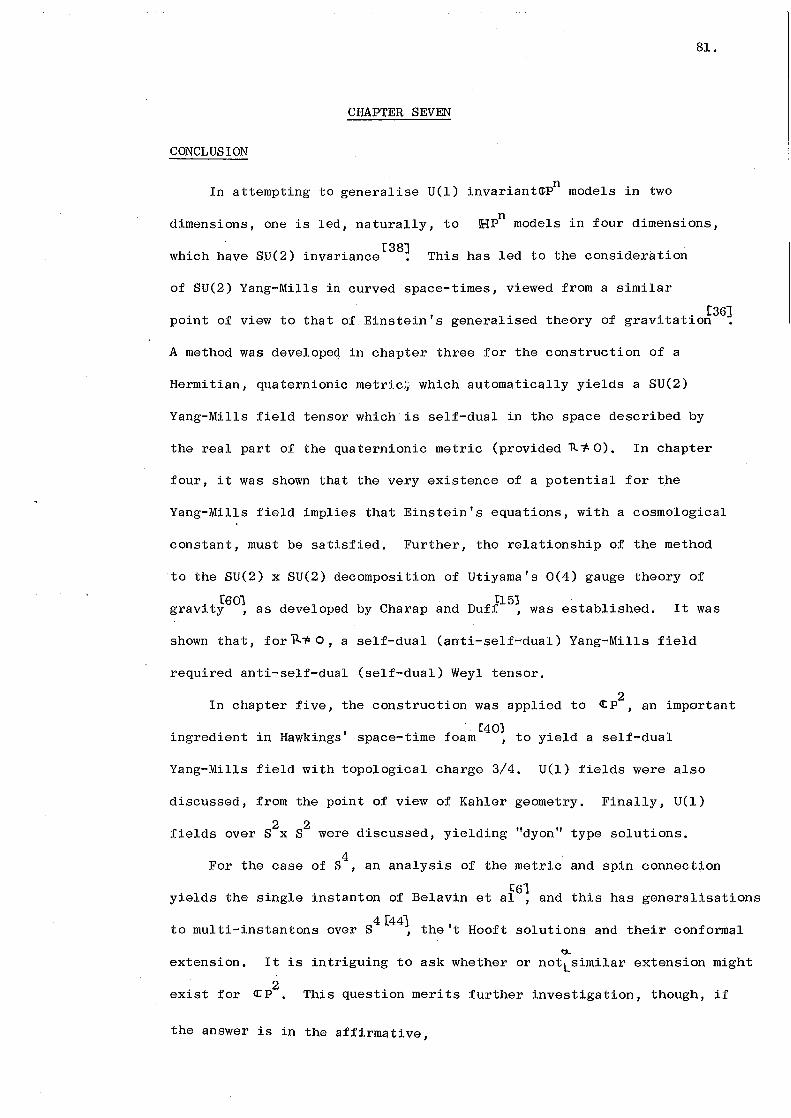
81.
CHAPTER SEVEN
CONCLUSION
In attempting to generalise U(l) invariant~Pn models in two
dimensions, one is led, naturally, to n EP models in four dimensions,
which h~ve SV(2) invariance[38~ This has led to the consideration
of SU(2) Yang-Mills in curved space-times, viewed from a similar
. . ' . d h f . t t . [ 36] po1nt of v1ew to that of.Einstein s general1se t eory o grav1 a 1on .
A method was developed in chapter three for the construction of a
Hermitian, quaternionic metric:; which automatically yields a SU(2)
Yang-Mills field tensor which is self-dual in the space described by
the real part of the qua ternionic metric (provided R 1- 0). In chapter
four, it was shown that the very existence of a potential for the
Yang-Mills field implies that Einstein's equations, with a cosmological
constant, must be satisfied. Further, the relationship of the method
to the SU(2) x SU(2) decomposition of Utiyama's 0(4) gauge theory of
. (601 [151 grav1ty , as developed by Charap and Duff , was established. It was
shown that, for R1= 0, a self-dual (anti-self-dual) Yang-Mills field
required anti-self-dual (self-dual) Weyl tensor.
2 In chapter five, the construction was applied to ~P , an important
[401 ingredient in Hawkings' space-time foam , to yield a self-dual
Yang-Mills field with topological charge 3/4. U(l) fields were also
discussed, from the point of view of Kahler geometry. Finally, U(l)
fields over s2x s2
were discussed, yielding "dyon" type solutions.
4 For the case of S , an analysis of the metric and spin connection
1:"61 yields the single instanton of Belavin et al , and this has generalisations
. . s4 [441 h ' f . to mult1-1nstantons over , t e t Hoo t solutions and the1r conformal
~
extension. It is intriguing to ask whether or notlsimilar extension might
exist for <CP2
This question merits further investigation, though, if
the answer is in the affirmative,

82.
it will not be easy to find. Compare the comple.xi ty of the single
instanton over ~P2 (5.41) to that of s4 (4.17).
Another important question is, how to extend this construction
to the real gauge symmetry of the strong interactions, S'U(3), since
this was our motivation for studying SU(2) in the first place - to
obtain a better understanding of SU(3). The work so far has
depended crucially on the relationship of quaternions to 8U(2) and the
fact that 0(4) ~ 8U(2) x 8U;2), the later being an accident of low
dimensional Lie group theory~ SU(3) is not a sub-group of 0(4), so it
is not obvious that the same methods will work for SU(3). However,
there is another accident of group theory, which could prove useful,
and that is 0(6) ~ 8U(4) ~ SU(3). An 0( 6) gauge theory could be
used to describe the curvature of a six dimensional manifold. The
6 simplest, compact, six dimensional manifold is the sphere S , which
is also an Einstein space. Thus one could ®onsider a SU(4) gauge
theory over 86 , whose connection is simply the spin connection of s6,
and try reducing this to a field over 84
by projecting out or compac-
tifying two of the dimensions.
AL,metric for 86
is
where~. v = l, .•• , 6
(.\+ ~'1.)1. (,
"V a. -- " "' "' _,.... ;;:,., .,....,... "'"JJ-
A choice of Vierbeins is
<...~=11"")'-).
The Christoffel symbols resulting from (l) are
(l)
(2)
(3)

83,
Thus the spin connection is
(4)
are the generators of 0(6),
The 0(6) field tensor is
~ <.. ~~'I ~ ~ ~ - 'b},... 3 i.. "Y ') CS" ~ ~
(.\+ -x."-)'l.. (5)
over
The configuration (4) and (5) can be considered as a 8U(4) field
with a- .. being (possibly complex) generators of 8U(4), l.J
The concept of self-duality does not apply in six dimensions,
but it is easy to check that, if one takes the six dimensional action
to be
and varies the potential to obtain the six dimensional Yang-Mills
equations
then (4) and (5) satisfy (7).
Unfortunately, it does not seem possible to obtain a 8U(4) field
over 84 from (4) and (5) in any simple way. If one tries to project
down onto 84
, or integrate over two of the co-ordinates so as to
eliminate them, one finds that nine of the generators are eliminated
also, leaving an 0(4) or 8U(2) x 8U(2) configuration over 84
, which
. h f 1 . l [61 Th . t . l h t 1.s exactly t at o Be av1.n et a . us 1. rema1.ns unc ear ow o
extend this formalism to 8U(3).
Another field of study, which has not been touched upon in this
(6)
(7)

'84.
thesis, is that of Yang-Mills - Higgs monopoles in curved space-times.
. ll6 18) Much work has been done on this subJect ' and though the topic
was investigated for this thesis, no further progress was made.

APPENDIX A - QUATERNIONS
Quaternions, or Hypercomplex numbers, were first considered
by Sir William Hamilton in 1843 in attempting to understand the
algebra of rotations. The quaternions have three basis elements
e1 , e2 , e3
which satisfy the algebra
= -1 (A .1)
A matrix r~presentation for such an algebra is given by the Pauli
matrices,
...12., = -1. [0 I J ~?w ~ -~I~ -~] IL~ 1:: -i [' 0] I 0 I 'L 0 0 -1
(A.2)
it is thus identical to the algebra of SU(2). This representation is
anti-he;rmitian ~ .
~;. =- .~t;,,"=l,'l.,;where <.t) means transpose followed by
complex conjugation. If we supplement (A.2) with the unit 2 x 2 matrix
then a general quaternion can be written as a linear
combination of the four matrices {~ 0 >~'>!1..1.,11.. ... 1
(A. 3)
where yJ~ , 'i.. = o, ... 1 ; are real numbers. The set of all such p form
a skew symmetric field, the field of qua tern ions, denoted by IE-I.
The magnitude of p is defined by
(A .4)
The set of quaternions of unit ma·gni tude is identical to the group
SU(2).
It is sometimes convenient to break quaternions up into their
real and pure quaternionic parts (den:oted by R 'fl and V...C. y> respectively).
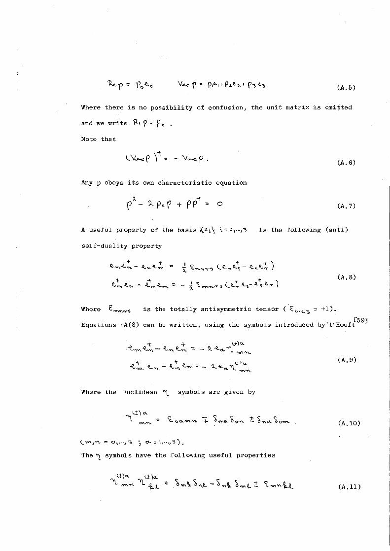
(A. 5)
Where there is no possibility of confusion, the unit matrix is omitted
and we write 'R.. r ; p C> •
Note that
(A. 6)
Any p obeys its own characteristic equation
(A. 7)
A useful property of the basis ~ .e.i-'1 'i, = o, ... 1 ~ is the following (anti)
self-duality property
t .Q....,..,.-t. ...... - -t
~-~ ...... -= I ~ -t ) -;:. £..,..,. ...... ~ l~ .... Q.. .. - ~ .. ~ .....
"t ;-I 'i. -T Q..i" ~ )
(A. 8) e....,~'\'\ .Q...,.,..Jt.""' -::- - ~ ,.,......,...,...-; <...e... ... ~-s- 'S ....
Where £....,...,.....5 is the totally antisymmetric tensor ( 't 01 ~"!> = +1).
[59] Equations ~A(8) can be written, using the symbols introduced by'ttHooft
(A. 9)
Where the Euclidean "!. symbols are given by
(A.lO)
The~ symbols have the following useful properties
(A .11)

L:!:.l Cl. U:) 'o '"Yt f'tY\rt'\. ~ 'WI~ =
In addition, the following properties sometimes prove useful
-I
~ =
t ~r
(A.l2)
(A.l3)
(A .14)
(A.l5)
(A.l6)
(A.l7)
Finally we note that points in four dimensional Euclidean spac.e-time
can be labelled by a single qua tern ion
(A .18)
For further details of quaternions and quaternionic valued functions
[381 f581 see references and .
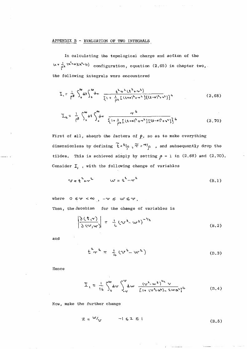
APPENDIX B - EVALUATION OF TWO INTEGRALS
In calculating the topological charge and action of the
I 1
i ) v.~ r'l. ~'JI.I-<>')l'X.T-b configuration, equation (2.65) in chapter two,
the following integrals were encountered
(2.68)
(2.70)
First of all, absqrb the factors of p, so as to make everything
dimensionless by defining t = ttr , :;: :: 'T'/p , and subsequently drop the
tildes. This is achieved simply by settingp = 1 in (2.68) and (2.70).
Consider Ir , with the following change of variables
'l.. '),. \jJ".:: t _.,...
where o ::; "l.r < ~
Then, the Jacobian for the change of variables is
'ld <.. t )"~'J \ ::-d 1,.''\1") \JV)
and
Hence
_,,'l. l. \_ v),.- w2.) 4
!!. 2. ,,'l.. tv-w) v
Now, make the further change
.... - w I "'- - '\)
(B.l)
(B.2)
(B.3)
(B.4)
(B.5)

and define
then
-:::: ~ (._\-1-'V"'+o-.4-) :l a.."" "'T
Consider, l "2. -:::: ~ 9)
We have the standard integral (Ref[351No. 331, 89b)
=
provided ~'.1. >b1 , which can be verified, for all 'IT, from (B.6).
Differentiating (B,9) with respect to r , with b =-1, gives
Substituting (B.lO) into (B.7) yields
Oo \ [U+O..."-)-t-v:l..J v-"d-'\J J0 ['v'~-+?...ll-o.4-)v2.+-U+O.II-)~5/'1..
Let 'X "'v:l. , and this splits up into
which again is a standard form (ref. [35)No," 213 ~a and Sb)
(B,6)
(B.7)
(B.8)
(B.9)
(B.lO)
(B .11)
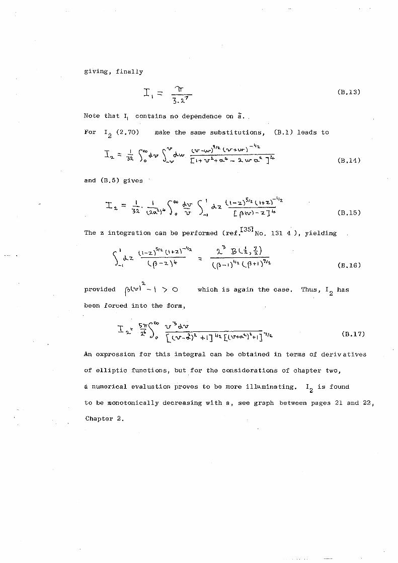
giving, finally
(B,l3)
Note that ~ contains no dependence on i.
For r 2 (2.70) make the same substitutions, (B.l) leads to
(B.l4)
and (B.5) gives
(B.l5)
The z integration can be performed (ref.[3~No. 131 4 ), yielding
(B.l6)
'l. provided [?~v) - \ ') 0 which is again the case. Thus, r
2 has
been forced into the £orm,
(B.l7)
An expression for this integral can be obtained in terms of derivatives
of elliptic functions, but for the considerations of chapter two,
a numerical evaluation proves to be more ill~minating. r2
is found
to be monotonically decreasing with a, see graph between pages 21 and 22,
Chapter 2.

REFERENCES
1. Actor A., Rev. Mod. Phys. 51 (1978) 461.
2. de Alfaro v., Fubini s., and Fur~an G., Nuovo Cimento 50A (1978) 523
3. Alvarez-Gaume L., and Freedman D.Z., Stony Brook pre-print (1980) ITP-SB80-31, "A Simple Introduction to Complex Manifolds"
4. Atiyah M.F., Drinfeld V.G., Hitchin N.J. and Manin Yu. I., Phys.Lett. 65A (1978)185
5. Atiyah M.F., Hitchin N.J., and Singer I.M., Proc.Roy.Soc.London A 362 (1978) 425
6. Belavin A.A., Polyakov A.M.,Schwartz A.s., and Tyupkin Yu.s., Phys.Lett~59B.(l975) 85
7. Berger M., Metz Conference Report (1979) Analyse SurLes Varietes, "Rapport Sur Les Varietes d 'Einstein" Societe Mathematique de France
8. Boutaleb~.routei H., Chakrabati A., and Comptet A., Phys.Rev.Dl9 (1979) 457
9. Boutaleb-Joutei H., Chakr~ati A., and Comptet A., Phys Rev.D.20 (1979) 1884
10. Boutaleb-Joutei H., Chakrabati A., and Comptet A., Phys Rev.D.20 (1979) 1894
11. Boutaleb-Joutei H., Chakrabati A., and Comptet A., Phys Rev.D.21 (1980) 979
12. Boutaleb-Joutei H., Chabrabati A., and Comptet A., Phys.Rev.D21 (1980) 2280
13. Boutaleb-Joutei H., Chakrabati A., and Comptet A., Phys.Rev. D21 (1980) 2285
14. Callan C.G., Dashen R., and Gross D.J., Phys.Rev.Dl7 (1978) 2717
15. Charap J.M., and Duff M.J., Phys.Lett.69B (1977) 445
16. Cho Y.M., and Freund P.G.o., Phys.Rev. Dll (1975) 2692
17. Close F.E., An Introduction to Quarks and Partons, (1979) Academic Press
18. Comptet A., Ann.Inst. Henri Poincar~, 23 (1980) 283
19. D'Adda A., Di Vecchia P. 1 and Luscher M. 1 Nucl.Phys.Bl46 (1978) 63
20. D'Adda A. 1 Di Vecchia P. 1 and Luscher M. 1 Nucl.Phys.Bl52 (1979) 125
21. Din A.M. 1 and Zakrzewski W. 1 Nucl.Phys.Bl74 (1980) 397
22. Din A.M. 1 and Zakrzewski W. 1 Phys.Lett.95B (1980) 419
23. Dolan B.P. 1 J.of Phys.A. Math.Gen. 14 (1981) 1205
;)
\ \
24.
25.
26.
27.
28.
29.
30.
31.
32.
33.
34.
35.
36.
37.
38.
39.
40.
41.
42.
43.
44.
4,5.
Dolan B .P., Durham University pre-print ( 1981), "Quaternionic Metrics and SU(2) Yang-Mills"
Eguchi T., and Freund P.G.O., Phys.Rev.Lett. 37 (1976) 1251
Eguchi T., Gilkey P.B., and Hanson A.J., Phys.Rep.66 (1980) 213
Eichenherr H., Nucl.Phys. Bl46 (1978) 215
Eilenberg s., and Niven J., Bull.Am.Math.Soc. 50 (1944) 246
Einstein A., Rev. Mod.Phys. 20 (1945) 35
Felsager B., and LeiQ~as J.M. Phys.Lett. 94B (1980) 192
Gibbons G.W., and Hawking s.w., Phys.Rev.Dl5 (1977) 2752
Gibbons G.W., and Pope C.N., qonun-Math.Phys.61 (1978) ·239
Gibbons G.W., and Pope C.N., Comm:.Math.Phys.66 (1979) 267
Golo V.L. and Perelomov A.M. Phys.Lett.79B (1978) 112
GriDbner W. , and Hofrei ter N. , Integral tafel, Bestinunte Integrale · ( 1961), Springer-Verlil.;g ·
Gi.irsey F., Yale University pre-print YTP 79-07 (1979), '\Geomet:dsation of Unified Fields"
Giirsey F., Jafarizadeh ·IVI.A., and Tze H.c., Phys.Lett.88B (1979) 282
Gursey F., and Tze H.c., Yale University pre-print YTP 79-02 (1979) "Complex and Quaternionic Analyticity in Chi. ral and Gauge Theories'! 11
H~vaty v., Geometry of Einstein's Unified Field Theory (1957) Noordhoff Ltd.
Hawking s.w., Nucl. Phys. Bl44 (1978) 349
Hawking s.w., and Ellis G.F.R., The Large Scale Structure of SpaceTime (1973), Cambridge University Press.
Hawking s.w., and Pope c.N., Phys.Lett. 73B (1978).42 .,
Hitchin N.J.; J.of Diff.Geom. 9 (1974) 435
Jackiw R., Nohl c., ~nd Rebbi c., Phys.Rev.Dl5 (1977) 1642
Jafarizadeh M.A., Snyder H., and Tze H.c., Yale University pre-print YTP 80-08 (1980), "Quaternionic Multi-s4 Instantons in General Co-variant SU(2) Yang-Mills and JHP n - models"
46. Kafiev Yu.N., Nucl.Phys. Bl78 (1981) 177
47. Kibble T.W.B., J.Math.Phys. 2(1961) 212
48. Kodaira K., Am. J. of Math. 86 (1964) 751
49, Lanczos c., Ann, of Maths. 39 (1938) 842
50, Misner c.w., Thorne K.s., and Wheeler J.A., Gravitation (1970), p.ll90, Freedman and Co.
51. Nahm W., CERN pre-print TH-2901-CERN (1980)
52. Neinast R.A., and Stack J.D., Illinois pre-print Ill-(TH)-80-6 (1980) "Non-Abebian Gauge Theory and cs-1\. <:s- models"
53, Page D.N., Phys, Lett.79B (1978) 235
54, Petrov A.z., Einstein Spaces (1969), Pergammon Press
55. Pope C,N., and Yuille A.L., Phys.Lett. 78B (1978) 424
56, Shaw R., "The Problem of Particle Types and Other Contributions to the Theory of Elementary Particles". Cambridge University Ph.D. Thesis,
57. Steenrod, N., The Topology of Fibre Bundles (1951), Princeton University Press
58. Sudbury A., Math,Proc. Camb, Phil.Soc. 85 (1979) 199
59. 'tHooft G., Phys.Rev.Lett 37 (1976) 8
60, Utiyama R., Phys. Rev,lOl (1956) 1597
61. Weinberg S., Gravitation and Cosmology (1972), Wiley
62. Wu T.T, and Yang C.N., Phys.Rev. Dl2 (1975) 3845
63. Yang C.N., and Mills R.L. Phys.Rev. 96 (1954) 191
64. Yano K., Differential Geometry on Complex and Almost Complex Surfaces (1965); Pergammon Press
Related Documents