DSP Lectures

1.1 PREAMBLE

We’ve set out this material as 24 chapters with a target of 10 pages per chapter. That should make each chapter "digestible" at asingle sitting. After 24 such sittings, you should know something about DSP. This brief and hopefully enticing recipe comes at aprice: it calls for great economy of words, and not much room for elaboration. The chapters may be short, but they demand yourfull attention. So be warned.

This chapter is introductory, with very little maths. It helps set the scene for what follows. We talk about the different kinds ofsignals, and about signal attributes such as power and energy. We talk about "frequency", and how signals have alternativedescriptions as "spectra". We note the role of signals in instrumentation and control. We say how signals are used forinformation transfer, and we mention some operations on signals, such as compression, enhancement, and encryption. We finishwith some comments on the analogue and digital technologies that make all of these things possible.

New Page 1

1

1.2 SIGNAL TYPES

In this section we categorise signals as analogue or digital signals, as pulses or periodic (i.e. repetitive) shapes, ascontinuous or sampled data types.

1.2.1 Signals Overview

The term signal refers to the quantitative measurement of parameters that interest us. Some signals, such as temperature,pressure, velocity, etc, are physical parameters, and we often record their variations over time. A velocity signal, for example,might be called v(t) where t is the time parameter. For any given t value, the function v(t) gives the velocity at that time. Thisv(t) is an analogue signal quantity that varies continuously over time.

Contrast this with a very different signal: the daily variations in currency exchange rates. The value of the Euro against the USdollar changes daily, and the "signal" is a sequence of numbers, one per day, that show the daily exchange rates. This signaltoo varies with time, but it is discrete rather than continuous, just one value per day. And, because it is a number, we probablythink of it as digital rather than analogue. Even analogue signals however, like velocity and temperature, can be convertedelectronically to digital form and then viewed numerically on a digital display panel.

New Page 1

2

Not all signals are functions of time. A surveyor will map out a building site as a function h(x,y) that shows the height at each(x,y) co−ordinate position. The signal is continuous, but the surveyor just records an adequate set of sample points and savesthem in numeric form for future use.

Some signals call for complex−number values. Wind velocity is a good example: it has both magnitude v and direction θ andwe can record it as v∠θ meaning "v angle θ". Both v and θ vary with time, so we should call it v(t)∠θ(t). In our work, we'llmeet lots of complex−valued signals, so we need to get used to the idea.

1.2.2 Analogue Signal Waveforms

Although many signals vary in irregular manner with no strong distinguishing features, the following distinction is very oftenapplicable:

1) signals that describe "one−off" events

2) signals that describe events which repeat over and over

New Page 1

3

Type 1) signals are transients or pulse waveforms, like the electric circuit transient shown here (Fig ë ). They have a shapethat happens just once. They frequently begin at a certain time instant (and are zero−valued before that). Some of themterminate and are zero−valued thereafter. Others decay slowly to zero but never quite reach zero. Their common feature is thatthey have finite area and "finite total energy" as we will shortly explain.

Here's a rather different pulse (Fig ç ). This probability density function p(x) is a pulse sure enough, but not a "time event" ofany kind. It too has finite energy, and for processing purposes, it is similar to many other pulse waveforms.

Type 2) signals are repetitive or periodic waveforms. Here (Fig ç) we see a portion of a periodic rectangular waveform. Itcould be a test signal from a function generator, or a clock signal on a digital circuit board. We see just a part of it, through afinite window width, but it is presumed to go on forever. That presumption simplifies the maths, since we don’t have tospecify how it starts or finishes. The same presumption applies to the waves that we call "sin" and "cos".

This (Fig í ) is another periodic waveform. It has a shape that we will encounter quite often. A single pulse of this kind iscalled a "sinc" pulse, and the periodic version shown here will be referred to as an "rsinc" waveform, where "rsinc" stands for"replicated sinc". Periodic signals have unlimited energy, but finite mean power. We'll elaborate shortly.

New Page 1

4

1.2.3 Replication and Periodicity

We can link pulses to periodic waveforms through a process called replication. The idea is that we can replicate a pulse andthus create a periodic "version" of the pulse. This is a pulse (Fig í ) that we call Π(t), pronounced "rect of t" for itsrectangular shape. It's got a height of 1.0 and an area of 1.0, so its width is W = 1.0 also (extending from −0.5 to +0.5). We'llmeet it often, so please note the definition.

We can replicate Π(t) at a replication interval P of our choosing. This plot shows the replicated Π(t) as Π(t)~ with interval

P = 1.5, (Fig ê ). Notice the ~ symbol on Π(t)~. We use this to mean replication or periodicity.

New Page 1

5

The pulse has been duplicated at regular intervals of P = 1.5 all along the axis. The result is the sum of such pulses, and itforms a periodic signal that goes on forever in both directions. Because we chose P > W, the pulses do not overlap, and wecan still see the rectangular shape of the original pulse. Replication is a very important concept in signal processing.

Here's another pulse (Fig ç ) called Λ(t) or "tri of t" for its triangular shape. It's got a height of 1.0 and an area of 1.0, so itswidth must be W = 2.0 (extending from −1.0 to +1.0). We'll meet it often, so please note the definition.

This plot (Fig ê ) shows the replicated triangle Λ(t)~ with replication interval P = 0.5. The pulse width is W = 2.0 and

now, because P < W, the pulses are overlapping, in fact we see multiple overlaps. The diagram shows us each of the

overlapping pulses, but Λ(t)~ is the sum of all these, and it turns out to be the constant level of 2.0 on the top of the diagram.

New Page 1

6

This tells us a lot about replication. First, if P < W, the pulses overlap and the original pulse shape is lost. Note carefully, we

can always build Λ(t)~ from Λ(t) once P is specified, but we cannot reverse the operation. The constant level of 2.0 tells us

nothing about the triangles that formed it. Other pulse shapes could give the same result, for example, a triangle of height 2and width 2, replicated at P = 1.0. We conclude that, when we replicated Λ(t), we lost information, and this is true in generalfor replication with overlap.

This plot (Fig ç ) shows Λ(t) in slices of width P = 0.5. Careful comparison against Λ(t)~ above during a one−period span

equalling P = 0.5 (the dotted rectangle) shows how Λ(t)~ is a superposition of all four slices. We just move all the slices

into the same one−period window and add them together. This has some interesting consequences:

the area within a one period window of the replicated pulse waveform equals the area of the original pulse.•

any window that is one period (P) in width can be used; sliding it to left or right has no effect.•

New Page 1

7

The window contains a stack of slices which, if laid out side by side, would re−assemble the original pulse. This is true evenfor pulses of unlimited width, such as the p(x) that we showed earlier. In such cases, we have an infinity of slices to add

together. We can't rebuild p(x) uniquely from p(x)~, but there remains a connection between them. That connection has

surprising importance in DSP generally, as subsequent chapters will reveal.

1.2.4 Sampled Data Signals

We cited the Euro exchange rate as a discrete data signal, just a sequence of numbers. In the computer−driven world of today,analogue signals too are routinely converted into number sequences, because computers work exclusively with numbers. Thisconversion calls for sampling of the signal x(t) at regular time intervals of T seconds as the diagram suggests (Fig ç ). Thesignal is sampled at times t = 0, t = T, t = 2T, t = 3T, and so on, and the sample values are converted to numeric form inan Analog−to−Digital converter, usually abbreviated as ADC or as A/D. The sample values are the values of x(t) at timest = nT, where n is an integer counter value, n = 0,1,2,3,4, .. etc. The value x(nT) is the vertical line length on the diagram.It's a numeric equivalent of the analogue signal level at that instant. The A/D converter gives us a stream of thesevalue−samples that describe the signal.

This diagram (Fig ç ) shows the same information as area−samples. Each area−sample gives the area of a slice of width T,such as the shaded slice in the diagram. It computes as T⋅x(nT), as opposed to x(nT) for a value−sample. Thereforearea−samples are just value−samples scaled by T, the sample interval. So why use them at all ? Well, first we can observe that:

New Page 1

8

The area is approximately the sum of the area−samples. The fact is, area−samples include T and thus retain the link with time,whereas value−samples are just a stream of numbers with no inherent time information. The usefulness of area−samples is at atheory level, where they help us retain the link between analogue signals and their sampled−data counterparts. This is quiteimportant because, when we sample a signal, we lose all the signal information between the samples.

We also noted a loss of information when we replicated a signal. Later on, we will discover a connection between replicationand sampling !

New Page 1

9

1.3 POWER AND ENERGY

Its time to say what we mean by power and energy. We'll use the AC mains voltage as an analogue signal example, but we'llextend our ideas to cover sampled−data sequences as well.

1.3.1 Analogue Signal Power and Energy

For an analogue time−signal x(t), we define the signal power very simply as:

Instantaneous power :

The power p(t) is indifferent to the polarity of the signal x(t), and it tends to emphasise the higher values of x(t). If weintegrate p(t) over the life of the signal, we get:

New Page 1

10

Total Energy:

This is a "global" measure of signal activity. With pulse waveforms, we can expect the integration to give a finite result, thatis, a finite value of total energy E. Not so with periodic waveforms. Because they go on forever, their total energy is infinite,and that's not a useful measure. The solution is to measure the energy over one cycle only:

Energy over one cycle:

where the upper−case P is the period of the waveform (or the duration of one cycle) in seconds. Then we can also specify themean power over a cycle as:

Mean power:

These concepts of power and energy are not unlike the true power and energy from which this terminology is borrowed. If x(t)were the voltage across a resistor R, then the instantaneous power in the resistor would be x2(t)/R, or p(t)/R as we have definedit. The only difference is in the factor R, but true power defines a very real heating effect as a rate of energy consumption,measured in Watts. The time integral of that activity is E, the energy used, which is also the total heat generated, in Joules.

New Page 1

11

The AC mains voltage provides a useful illustration. We can specify it as:

for a typical European distribution system. The angle α is the signal angle at the time we choose to call t = 0. Any angle willdo. This is known as a "220 volt" mains, although its peak value is 311 volts. There's a reason for this, as follows.

This plot (Fig ç ) shows a few cycles of the actual mains voltage, v(t), and underneath (Fig í ) is a plot of the"instantaneous power" as we define it in signal theory, that is:

in watts

The power waveform goes from a minimum of zero to a maximum of M2, the peak value squared. It is a "raised cosine" shape,with a frequency of 100 Hz. Every half−cycle of the voltage equates to one full power cycle. It is obvious from the shape ofthe power wave that the average power is one−half of the peak power:

watts into 1 Ohm

New Page 1

12

We like to specify the sinusoidal mains in such a way that this average power (into R = 1Ω) equals the voltage−squared, justas it is for DC voltages. Thus, the voltage is the root of the mean power, and we say:

This voltage is "the root of the mean of the squared waveform", hence the abbreviation "rms" that describes it. In ACtrue−power calculations, when the resistor R is included, it enables us to make statements such as:

− just as we would do for a DC circuit. Thus, the resistance of a 1 kilo−Watt heater element is just R = 2202/1000 = 48.4Ω. The rms value of 220 volts is the significant quantity as far as power usage is concerned. Then the rms current is calculatedas 220/48.4 = 4.5 Amps. In the signals context, and for future reference, we should remember that the mean power of asinusoid is M2/2, or one−half of the peak−value squared.

Compare this with the mean value of mains voltage v(t): taken over one or more cycles, the mean value is zero, which rendersit useless as a "global" measure of signal activity. The power, by contrast, is v(t)2. It is always positive, its integral is alwaysincreasing, and it works well as the global measure that we require.

The idea of power is very useful for a noise signal. We don't know the noise value at any given time, but we can still quantifyit in terms of its mean power, and thus decide whether it is large enough to be objectionable.

New Page 1

13

1.3 2 Sampled Data Power and Energy

When a signal x(t) is sampled, with T seconds between samples, the sample values are x(nT) for n = 0,1,2, …etc. Wesimplify our notation by calling them x[n], the same sequence of numbers, but with no mention of T.

Signal power x2(t) is an instantaneous thing, and so the sample power becomes x[n]2, with no time dependency. Energy,however, is (power × time), so we should think of the energy per sample as T⋅x[n]2. In practice, we often drop the T, thusignoring the time aspect, but still obtaining a useful global measure. The total energy of a sampled signal is thereforeT⋅Σx[n]2 (summed over all samples), or just Σx[n]2 if we ignore the time factor. We would then find the mean power over

N samples as either T⋅Σx[n]2/(NT), or as Σx[n]2/N when T is ignored. Either way, the mean power is independent of the sampleinterval T.

New Page 1

14

1.4 TIME AND FREQUENCY DOMAINS

A great deal of DSP work is about signals that change over time, but in our efforts to describe them, we also speak offrequencies, such as the 50 Hz frequency of the AC mains. Such references are hard to avoid. They are part of an alternativeviewpoint that we can bring to bear on a signal. We can describe a signal fully in the time domain, or equally well in thefrequency domain. Each description has its good and its bad features, but the frequency approach is of such importance that itruns all through this work, and through most books on signal processing. We will try to expain the differences in theseapproaches.

1.4.1 Time versus Frequency

The time description of our mains voltage might have been:

New Page 1

15

(We tend to use x(t) for analogue time signals generally). This time−domain description is the collection of all possible signalvalues. We've drawn it alongside over a 60 milli−second time window (Fig ç ). Even a rough plot of x(t) requires severaldata points to convey the general shape.

There's a simple alternative, as this diagram illustrates (Fig ç ). We can just say:

This is the frequency−domain description. It says just as much as the time−domain description, but it says it more compactly.The X(f) plot needs only a single complex−number value placed at f = 50 Hz. Its magnitude is 311, the cosine peak value,and its angle is the initial angle of 0.2 radians (when t = 0).

But what of other signal shapes ? Actually, this method would not be much good were it not for the fact that we can constructany shape we please from a sum of sine waves. We'll see the evidence of this as we continue. We can thus have a spectraldiagram X(f) that shows one complex number for each sine wave that makes up the signal.

New Page 1

16

In the future, we can describe our signals as x(t), the time−domain view, or alternatively and equivalently as X(f), thefrequency−domain view. If we know x(t), we can find X(f) and vice versa. Indeed, the two are linked by a transform (formula)known as the Fourier Transform (FT). There are different FT's to suit different signal types, as follows:

The Continuous Fourier Transform (CFT) is for analogue time pulses.• The Discrete−time Fourier Transform (DtFT) is for sampled time signals, or for number sequences.• The Discrete−frequency Fourier Transform (DfFT) is for periodic time signals, like the sine wave that we mentioned,and these signals are represented by a number sequence in frequency.

•

The Discrete Fourier Transform (DFT) connects data samples in time to data samples in frequency. It is a fully digitaltransform, and is widely used to do calculations by computer.

•

These transforms are developed over the next two chapters. They will allow us to work interchangeably in the two domains.The DFT works only with numbers, making it ideal for computer use, and it has a fast version that we call the Fast FourierTransform (the FFT). Not only does it switch quickly between the domains, but it can speed up various number−crunchingjobs, doing them much more rapidly than would otherwise be possible. The FFT is the workhorse of signal processing, and isvery widely used.

New Page 1

17

1.5 TECHNOLOGY REVIEW

As recently as 1970, digital signal processing was a little known area, just beginning to emerge. Thirty years later, in the year2000, its effects were everywhere to be seen, in music, in computers, in communication, and about to conquer television aswell. And the world wide web had arrived, persuasive evidence of an emerging "Information Age". We will take a briefglimpse backward over this era of extraordinary development.

1.5.1 The Early Days

The technology of world war two was high technology, for its time, with impressive achievements in electronics, in spite of avery limited technology base. Radio communication had arrived, and signal processing had commenced, with signals rangingfrom morse code through analogue radio signals to the early radar signals and, of course, everything was done usinganalogue techniques. The bipolar transistor had not yet arrived, and thermionic valves provided the link into the future. Thesewere soon made obsolete by the transistor, which for many years prospered as a stand−alone three−terminal device. With thetransistor, analogue design methods flourished, and quite a lot could be done with just a small number of these devices. Rapidprogress in radio and in television provided ample evidence of all this.

The first experimental computers used thermionic valves, and the transistor soon transformed them into serious computingmachines, but in a price range that was affordable to big business, and to military users, but not to many others. All that began

New Page 1

18

to change with the arrival of the integrated circuit.

1.5.2 Development Milestones

The planar integrated circuit (IC) was introduced by Robert Noyce in 1959, making it possible to build and to interconnectmany devices simultaneously on a single "chip", and to reproduce these circuits easily and in quantity. The IC set the scene forthe accelerated growth which followed.

Nine years later, Noyce joined with Gordon Moore to start the Intel Corporation in Santa Clara, California. The firstmicroprocessor was built by Intel in 1971, and it heralded the beginning of the personal computer era. The early highlights ofthis era included the appearance of the Apple II in 1977 and the IBM PC in 1981.

The microprocessor is a general−purpose binary machine, with logic and arithmetic capability. Typical microprocessors canadd and subtract in a single machine cycle, but a multiplication involves many such steps, and must be expressed as a softwareroutine that takes several machine cycles to execute.

This approach is too slow for a majority of DSP tasks that must operate in real−time. Fast multipliers are a priority, and this isa primary distinction between DSP processors and other processors. DSP processors have their own internal multiplier"engine", implemented in silicon, and can generally complete a multiplication in a single machine cycle.

Multipliers have come a long way, from the multipliers of the seventies which filled complete circuit boards, to thesingle−chip multipliers of the eighties, and to the vastly reduced geometries of the nineties. The time to perform amultiplication has fallen dramatically as well, from several hundred nanoseconds for the board−level products to less than 20nanoseconds in 1997. This latter figure is a mere 20×10−9 seconds, and its reciprocal is 50×106. This multiplier could execute50 million multiplications per second !

New Page 1

19

1.5.3 Here and Now

Looking back a quarter century or so, the DSP of that time had few engineering roles, and very little impact that we could see.In the interim, everything has changed. That change is largely due to the advent of fast inexpensive digital technologies. Themost visible manifestation of change is in the proliferation of computing equipment. But, alongside these advances, a greatmany analogue engineering functions have been replaced by new digital counterparts. Most information flow is now in digitalform. This includes audio information, which is now mostly digital, and digital video signals, which are not far behind.

The migration to digital is limited by two main factors: cost and speed. As the cost of digital functions continues to fall, mostof the remaining analogue systems will become obsolete. Speed is a more significant limitation, and certain specialised highfrequency processes will continue in analogue form for a long time to come.

This does not alter the fact that we already live in a mostly digital world, and the current boundaries between radio, television,telephones, computers, etc are being eroded. We face a new era in which all these systems, and more, are just differentmanifestations of information transfer and processing.

New Page 1

20

1.6 DSP TODAY

In this section, we will take a brief glimpse at the signal processing operations of today, the parameters that interest us, and theunderlying motivations.

1.6.1 Signal Monitoring Tasks

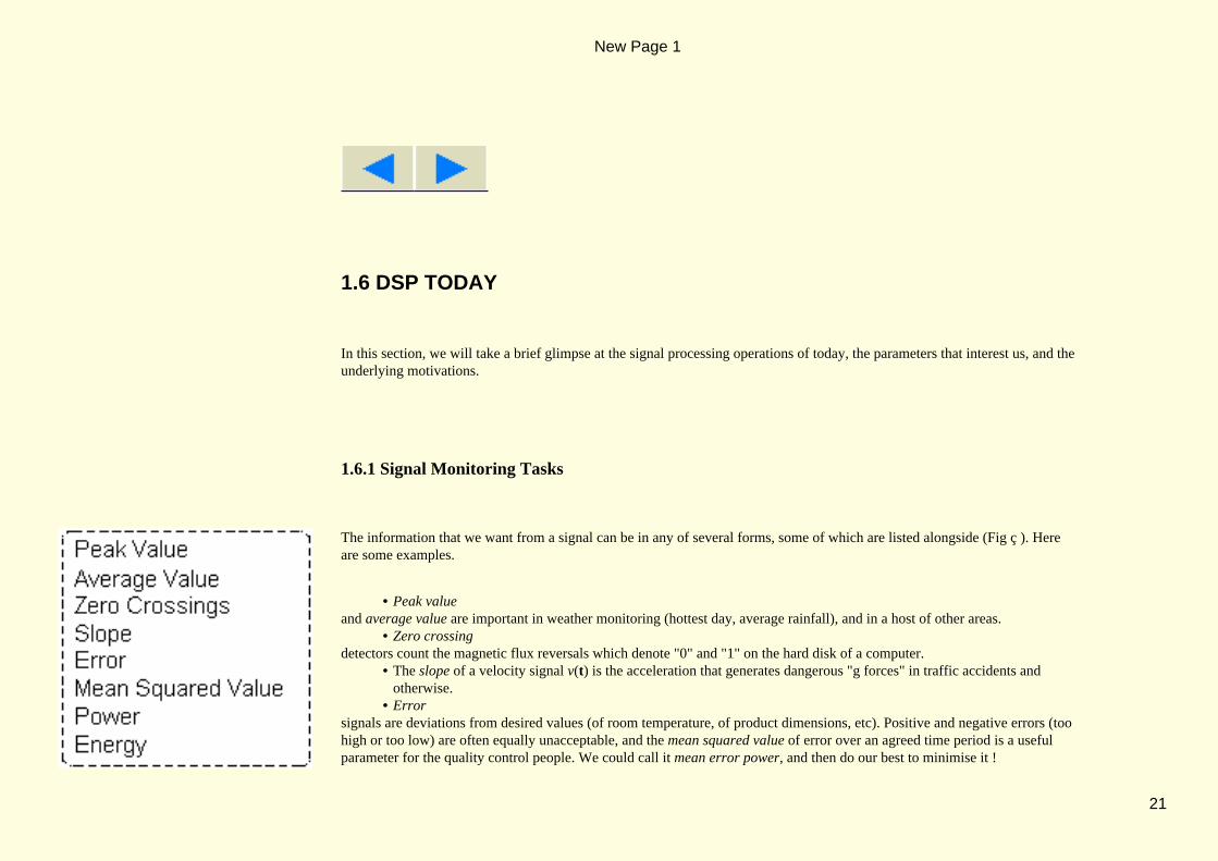
The information that we want from a signal can be in any of several forms, some of which are listed alongside (Fig ç ). Hereare some examples.

Peak value• and average value are important in weather monitoring (hottest day, average rainfall), and in a host of other areas.

Zero crossing• detectors count the magnetic flux reversals which denote "0" and "1" on the hard disk of a computer.

The slope of a velocity signal v(t) is the acceleration that generates dangerous "g forces" in traffic accidents andotherwise.

•

Error• signals are deviations from desired values (of room temperature, of product dimensions, etc). Positive and negative errors (toohigh or too low) are often equally unacceptable, and the mean squared value of error over an agreed time period is a usefulparameter for the quality control people. We could call it mean error power, and then do our best to minimise it !

New Page 1

21

1.6.2 Signal Processing Tasks

The list is a very long one, but we will try to give some small impression of the tasks to be done and the reasons that motivatethem.

Virtual Instrumentation. Instead of using dedicated oscilloscopes, spectrum analyzers, and other instruments, we can use anADC to digitise a signal, then do all the processing on a computer, while using the computer screen as the instrument displaypanel.

Systems Control. A primary reason for monitoring a signal is so that we can make corrections, as when we measure roomtemperature and use the information to adjust the supply of heat. This is as simple form of feedback control system. Controlsystems abound in industrial applications.

Filtering. A filter modifies a signal by blocking some of its frequency components and allowing the rest to go throughunaffected.

Noise Removal. Some filters are for the removal of unwanted noise signals. Narrow−band noise is often easy to remove.Broadband noise is more challenging.

Information Transfer. This covers a multitude. Even "local transfers", such as the transfer of data from a Compact Disk(CD) or Mini−disk (MD) to the music output circuitry can involve complex line codes and de−compression algorithms. Longdistance transfers are made over the air waves, or through co−ax cables, or through fiber−optic cables. These involvemultiplexing methods (in time or in frequency) so that several signals can share the same path, modulation methods whichplace the signal in a frequency band that suits the transmission medium, and de−modulation methods that restore the originalsignal at the receiver. All this applies to telephone, radio and television links, both analogue and digital, and to the world−wide

New Page 1

22

web links, which are exclusively digital.

Signal Enhancement. This includes making noisy voice recordings more intelligible, and making blurred video images morerecognisable. There are many techniques, and they use digital processing for the most part.

Signal Compression. This reduces the data length with little or no damage to the content. With lossless compression methods,we can restore the original data exactly, but compression factors of 2 to 4 may be all we can achieve. With lossy compressionmethods, full restoration is impossible, but that is often unimportant, as with audio or video data, provided the final sound orimage seems satisfactory. Lossy compression can achieve far higher compression ratios, as much as 10 to 50 times, but withsome loss of quality as the ratio increases. There are two main benefits from data compression: less space is needed to storethe data, and less time (and cost !) is needed to send it over a data link. Compression is sometimes a necessity: without it,digital television transmissions would not be viable.

Message Encryption. The internet (and private intranets) make communication easy, but they also create a need for datasecurity. The answer is to encrypt a message before transmission, which makes it unintelligible, and to reverse the processlater. The methods are mostly digital, and highly sophisticated.

1.6.3 Digital Versus Analogue.

Some of the listed operations have used analogue methods in the past, particularly systems−control, filtering and informationtransfer. Now, more and more, they use digital methods instead. We will briefly set ot the reasons for the changeover.

Analogue methods are subject to large component variations over process and over temperature, making it verydifficult to achieve high precision. With digital methods, the precision is limited only by the word−length employed.

•

Analogue design can be difficult and time−consuming. Digital soultions are getting less and less expensive, smallerin size, and easier to automate.

•

Digital solutions have great immunity to noise. In a digital phone link, a signal will pick up noise along the way, butthe binary digital data (0's and 1's) can be fully re−constituted and rendered "noise−free" again (except in extreme

•

New Page 1

23

high−noise conditions).Analogue solutions serve one purpose only, but digital solutions are highly re−configurable. The ultimate example isthe computer. It re−configures itself for a new role every time we open a new application.

•

That leaves only a few categories in which analogue methods win out. At very low price levels, an analogue solution may becheaper, and still suffice (cheap radios, etc). For very high−speed systems, the digital option may be too slow, and ananalogue solution must be used. And finally, at the Analogue/Digital interface (in A/D and D/A converters), some analoguecircuitry cannot be avoided.

1.6.4 Algorithms and Implementations.

There are two distinct parts to a problem: the algorithm and the implementation. The algorithm is the mathematical strategy,and it applies to both analogue and digital solutions, although the word algorithm most often refers to software.

The implementation refers (mainly) to the hardware employed. The resistors, capacitors, transistors, etc, of the analogueimplementation give way to logic circuits in the digital implementation. The algorithm defines the result that we want, but theway that we get that result will depend on the implementation.

The algorithm is the concept side, and is relatively unchanging. The implementation is decided by technology, and can changequite rapidly. This book is mostly about algorithms. Our references to implementations are mostly for illustration, and to givea more practical bias to the work.

The future of electronics is mostly about information, and with less reason to separate the various audio, video, and otherinformation systems. We will see some merging of traditional roles, and a growing reliance on computers, while commercialfirms compete to define the shape of things to come.

New Page 1

24

New Page 1

25

2.1 PREAMBLE

First we show how to describe signals, both as maths expressions, and as pictures of waveforms. We explain signal symmetry.We introduce phasors, their properties, and we show how two phasors make a sine wave. We discuss sums of sine waves, andhow periodic signals are built from sine waves. Then we switch to a spectral viewpoint, and we show how to find the phasorsin a periodic signal. We arrive at the Discrete−time Fourier Transform, better known as Fourier Series.

New Page 1

26

2.2 SIGNALS IN TIME DOMAIN

Now we revisit the pulses, the replication, and the periodic signals of Chapter 1, but from a more mathematical viewpoint, thatallows precise descriptions.

2.2.1 Sketching Signal Waveforms

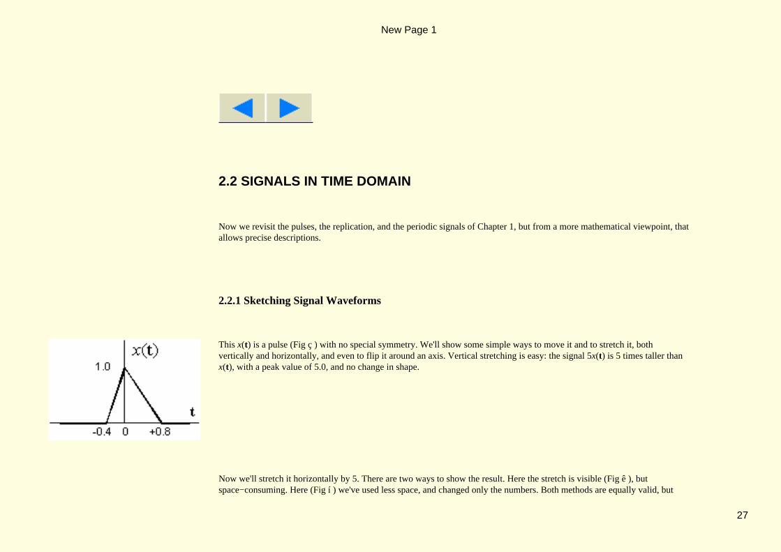
This x(t) is a pulse (Fig ç ) with no special symmetry. We'll show some simple ways to move it and to stretch it, bothvertically and horizontally, and even to flip it around an axis. Vertical stretching is easy: the signal 5x(t) is 5 times taller thanx(t), with a peak value of 5.0, and no change in shape.

Now we'll stretch it horizontally by 5. There are two ways to show the result. Here the stretch is visible (Fig ê ), butspace−consuming. Here (Fig í ) we've used less space, and changed only the numbers. Both methods are equally valid, but

New Page 1

27

we'll usually opt for the space−saving method.

Watch how the maths label has changed. It now reads x(t/5). To explain, x(t) comprises a function x() with a parameter,normally t, inside the brackets. We give a parameter value to x(), and x( ) gives us back a function value. By changingthe parameter to t/5, we now need a t which is 5 times larger to get the same parameter value. This stretches the x−shape by 5on the time axis. We could compress it by 5 in a similar way by using x(5t) as our new function.

To flip x(t) around its horizontal axis, we just take −x(t). This reverses the sign but not the magnitude for all values of t. Toflip x(t) around its vertical axis, we take x(−t) instead, as shown here (Fig ç ). The positive−t axis becomes thenegative−t axis and vice versa. This is time−reversal, and we will meet it occasionally.

To slide a signal along the t−axis by τ seconds, we use x(t−τ). Here we see a plot of x(t−0.4), representing a 0.4−sec timedelay (Fig í ). In x(t−0.4), t has to be greater by 0.4 to give the same parameter value as x(t), and this explains theright−shift. The function x(t+0.4) performs a 0.4sec left−shift, or time advance.

New Page 1

28

This (Fig î ) is a plot of x(t), and two copies of x(t), shifted right and left by a distance of P = 2. It looks periodic, but thereare 3 periods only.

To make it truly periodic, we must add more pulses to left and right ad infinitum. Here are a few of those pulses:

The fully periodic signal would be:

New Page 1

29

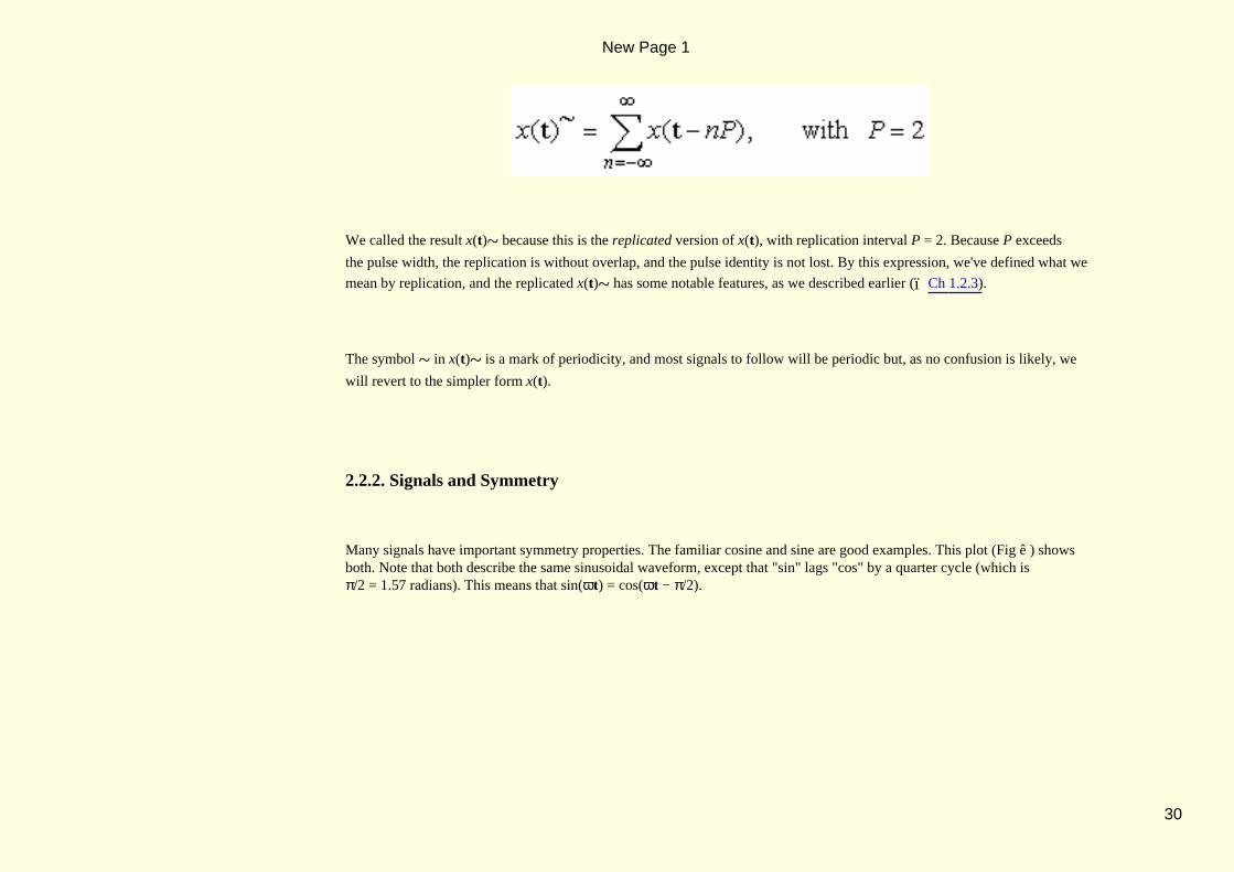
We called the result x(t)~ because this is the replicated version of x(t), with replication interval P = 2. Because P exceeds

the pulse width, the replication is without overlap, and the pulse identity is not lost. By this expression, we've defined what we

mean by replication, and the replicated x(t)~ has some notable features, as we described earlier (ï Ch 1.2.3).

The symbol ~ in x(t)~ is a mark of periodicity, and most signals to follow will be periodic but, as no confusion is likely, we

will revert to the simpler form x(t).

2.2.2. Signals and Symmetry

Many signals have important symmetry properties. The familiar cosine and sine are good examples. This plot (Fig ê ) showsboth. Note that both describe the same sinusoidal waveform, except that "sin" lags "cos" by a quarter cycle (which isπ/2 = 1.57 radians). This means that sin(ωt) = cos(ωt − π/2).

New Page 1

30

We've called the cosine wave xe(t) because of its even symmetry about the vertical zero−axis. We've called the sine wave xo(t)because of its odd symmetry about the same axis. These symmetries are defined by saying:

A given (real−valued) x(t), such as this one (Fig ç ), might have neither symmetry, but we can routinely decompose it intoeven and odd parts. Its even part is:

New Page 1

31

Notice, the right−hand−side (rhs) of the equation is unchanged if we use −t in place of +t.. This proves that xe(−t) = x e(t) asper the definition. The odd part of x(t) is found as:

Notice, the rhs of this equation is sign−reversed if we use −t in place of +t. This proves that xo(−t) = −x o(t) as per thedefinition.

To illustrate the method for the x(t) given above (Fig ë ), we've also shown x(−t), and we've sketched the xe(t) snd the xo(t)that result from our equations (Fig ç ). All plots use the same scale factor. Take a moment to check that they make sense.

Periodic signals likewise can have even or odd symmetry. The rectangular waveform (ï Fig 1.x.x) has even symmetry if weplace the t = 0 axis on the middle of the pulse (or midway between pulses), but not otherwise.

New Page 1

32

2.2.3 Phasors, Sines and Cosines

A vector can be described as L∠θ meaning "length L at angle θ". This is shorthand for the maths expression L⋅ejθ, becauseejθ is a vector of length 1 at angle θ. A vector that rotates at some uniform rate, call it f1 (in units of cycles per second orHertz), is a phasor of frequency f1.

A sinusoid of frequency f1 can be traced out as the projection of this rotating vector, or phasor, (which also explains why arotating turbine−generator yields a sine−shaped mains voltage). It resembles a wheel, rotating as:

where α is the initial angle at t = 0.The horizontal projection of w(t), as w(t) rotates, is seen here (Fig ç ). This sine−shapedx(t) is the real part of w(t).

the real part of w(t)

Note that the vertical projection is the imaginary part of w(t), or Imw(t), and both parts are featured in this well−knownrelationship:

New Page 1

33

The cos is the real part; and the sin is the so−called imaginary part. We'll use these ideas whan we talk about band−passsignals. Another way to generate a sine wave is based on the sum of a vector v and its complex conjugate v*.

If v = L∠θ then v* = L∠−θ and v + v* = 2Lcosθ

New Page 1

34

This diagram (Fig ç ) explains how it works. For a phasor, θ becomes (2πf1t+α), and it increases uniformly over time. Wecan then generate x(t) as:

This combines two phasors, both of length ½, to form a unit−amplitude sinusoid. The first phasor rotates (positive,anti−clockwise) at frequency +f1 with initial angle of +α. The second rotates (negative, clockwise) at frequency −f1 withinitial angle of −α. This diagram (Fig ç ) shows the individual phasors. Below (Fig í ) we see how the phasor sum isreal−valued (horizontal), and its length is the height of the sinusoid at that same instant.

New Page 1

35

This phasor sum (Fig é ) is the general sinusoid, and can have any value of initial angle α. The signals "cos" and "sin" (ï Fig2.2.2…1) are special cases. Setting α = 0 gives us cos(2πf1t). Its vectors are horizontal at t = 0 (Fig é ), and they add to1.0, the cosine peak at that same instant. Setting α = −π/2 gives us sin(2πf1t). Its vectors are vertical at t = 0 (Fig é ), andthey add to 0.0, which marks the positive−going zero−crossing of the sine at that instant. We prefer to write sin(2πf1t) ascos(2πf1t−π/2), since this identifies the angle correctly. That makes the "sin" somewhat redundant.

We've shown how signals can be advanced or delayed, or even flipped about the time axis. Its of some interest to see how asine wave would respond. We'll take time reversal first. Suppose x(t) = cos(2πf1t+α). Then x(−t) = cos(2πf1(−t)+α) whichis the same as saying x(−t) = cos(2πf1t−α) because the cos is even (cos(−θ) = cosθ). The effect of time reversal is tochange the sign of α. This plot offers graphical confirmation of that idea (Fig ë ).

New Page 1

36

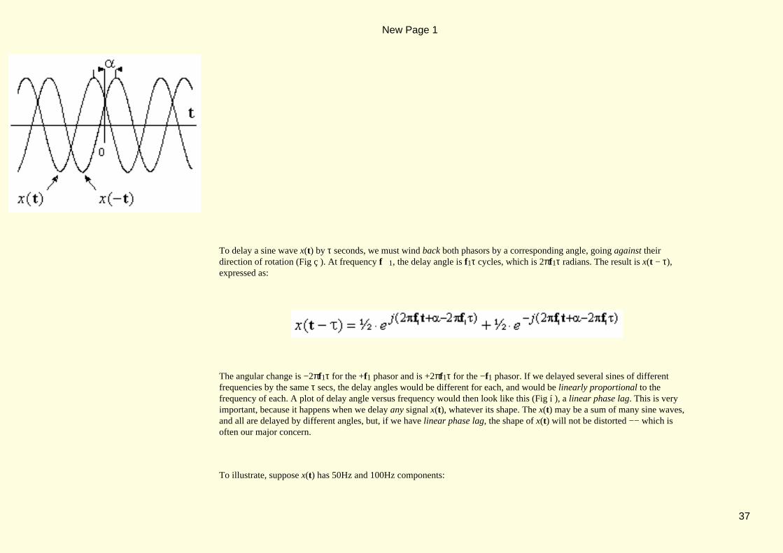
To delay a sine wave x(t) by τ seconds, we must wind back both phasors by a corresponding angle, going against theirdirection of rotation (Fig ç ). At frequency f1, the delay angle is f1τ cycles, which is 2πf1τ radians. The result is x(t − τ),expressed as:

The angular change is −2πf1τ for the +f1 phasor and is +2πf1τ for the −f1 phasor. If we delayed several sines of differentfrequencies by the same τ secs, the delay angles would be different for each, and would be linearly proportional to thefrequency of each. A plot of delay angle versus frequency would then look like this (Fig í ), a linear phase lag. This is veryimportant, because it happens when we delay any signal x(t), whatever its shape. The x(t) may be a sum of many sine waves,and all are delayed by different angles, but, if we have linear phase lag, the shape of x(t) will not be distorted −− which isoften our major concern.

To illustrate, suppose x(t) has 50Hz and 100Hz components:

New Page 1

37

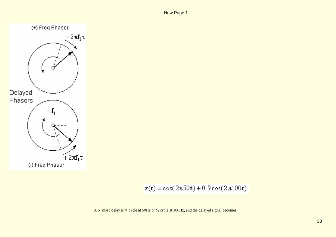
A 5−msec delay is ¼ cycle at 50Hz or ½ cycle at 100Hz, and the delayed signal becomes:

New Page 1

38

We can leave it like this, or re−write it as:

Either way, x(t) and its delayed version xd(t) look like this (Fig ç ). There is no change in shape. Signal integrity has beenpreserved.

2.2.4 Sums of Sine Waves

New Page 1

39

We can build arbitrary signals from sine waves. The following is a sum of N sine waves, all of different amplitudes Mk,frequencies fk , and angles αk :

Almost any result is possibe, but if we limit our options, it becomes more interesting. One way is to use the samefrequency f1 for all.

The magnitudes and phase angles are still arbitrary, but the sum x(t) is far from arbitrary. It is still a sine wave, and offrequency f1. We can find its peak value Mx and its angle αx from the relationship:

New Page 1

40

To understand why, recall that the phasors which make up the sine waves are all rotating together at the same frequency.Relative to one another, they are stationary. That's why we can add them all as vectors to get this result. In strict mathsnotation, we must replace ∠θ by ejθ everywhere. This is the method that we use in AC circuit theory. We can treat all voltagesand currents as vectors, because they all have the same frequency, and when they add they retain their sinusoidal shape. Youcan't say that about other waveforms (square, triangle, etc).

Moving on from just one frequency, we will allow different frequencies fk, but with this constraint:

The permitted frequencies are integer multiples of ε, where ε is the fundamental frequency. The result is a periodic x(t) ofperiod P such that:

The sinusoid of frequency fk = k ⋅ε is called the k−th harmonic component. The shape of x(t) is decided by the Mk and theαk of the various harmonics, noting that rapid changes in x(t) call for high harmonic frequencies. It turns out that any periodicx(t) of period P can contain the harmonic frequencies fk = k ⋅ε, where ε = 1/P, and only those frequencies. This diagram(Fig ê ) explains why. It shows the first and third harmonic components of an x(t) that repeats itself in windows of width P.The third harmonic has a period of P/3, but more importantly, it is also periodic in P, that is, it repeats identically insuccessive windows. This is essential for periodicity, and only harmonic frequencies have this property.

New Page 1

41

Notice, we allowed for a k = 0 term. This is a zero−frequency or DC component. It's action is to raise or lower the waveformby a fixed amount, and that does not affect the periodicity.

New Page 1

42

k Mk a

k

0 0.250 0

1 0.450 −45

2 0.318 −90

3 0.150 −135

4 0.000 −180

5 0.090 −45

6 0.106 −90

7 0.064 −135

8 0.000 −180

2.3 SIGNALS IN FREQUENCY DOMAIN

We can assemble a periodic x(t) of arbitrary shape by specifying its various harmonic components. The shape of x(t) over aperiod is the time−domain view. The list of harmonics (Mk, αk), is an alternative view, a frequency−domain view, or aspectral view, which we will now present.

2.3.1 Periodic Signal Spectra

This table (Fig ë ) is a list of (Mk, αk) values up to the tenth harmonic. We can build the waveform that it describes as:

New Page 1

43

9 0.050 −45

10 0.064 −90

When we do this, we get the waveform shown here (Fig ç ). It resembles a rectangular waveform of amplitude 1.0 andperiod P = 1.0, with pulse−width 0.25. The waveform repetition frequency is ε = 1 Hz. The highest frequency present is10 Hz, the 10−th harmonic, and this limits the available steepness at pulse edges.

The table of (Mk, αk) values is more often seen pictorially as a line spectrum such as the single−sided line spectrum shownhere (Fig ç ). We have a set of line lengths describing Mk values, and a separate set for αk values (now in radians), withfrequencies identified by k on the horizontal axis. Each (Mk, αk) pair describes one of the sine waves that make up the signal.

But the sine is not the most basic signal element. Each sinusoid is a sum of two conjugate phasors. The phasor of frequency+fk = k ⋅ε can be represented as:

New Page 1

44

The phasor of frequency −fk = −k ⋅ε can be represented as:

Notice how |C−k| = |C k| = ½M k, but argC−k = −argC k) = −αk, where "argC k" just means "the angle of Ck". Thek−th harmonic becomes:

New Page 1

45

There may be more here than meets the eye. Mk and αk are real numbers, but Ck and C−k are complex numbers whose anglesgive the phasors their initial phase. We could also write this k−th harmonic as:

The angles combine by addition:

We can eliminate C−k by using |C−k| = |C k| and argC−k = −argC k :

The |Ck| is now common to both, and since (ejθ + e −jθ) = 2cosθ, we get:

New Page 1

46

This is the k−th harmonic. The complete x(t) is the sum of the DC term and all of the harmonics, resulting in:

Or, equivalently, we could just add all the phasors to give:

This very compact form includes the DC term C0 at k = 0, while the phasors combine in pairs at k = ±1, k = ±2, k = ±3,etc to build the sine−wave components. Note that C0 = M 0 is the (real) DC level, but all other Ck are complex, with only halfthe length of Mk . We can have any number of harmonics, so we've extended the sums to infinity.

If we think in terms of phasors, then we will display the phasors on a double−sided spectrum, such as that shown below(Fig ê ), for the same rectangular waveform as before. This spectrum shows the negative frequencies too, and somesymmetry rules apply. Because |Ck| = |C −k|, the magnitude plot shows even symmetry about the vertical zero−axis. BecauseargC−k = −argC k, the phase plot shows odd symmetry instead. The spectra of real−valued signals will always have

New Page 1

47

these symmetries. That makes it frequently unnecessary to use a two−sided spectrum, since one side tells us all that we need toknow. But there are advantages in doing so, and this will be more apparent as we progress.

k Mk a

k

0 0.250 0

1 0.450 −45

2 0.318 −90

3 0.150 −135

4 0.000 −180

5 0.090 −45

6 0.106 −90

7 0.064 −135

8 0.000 −180

9 0.050 −45

10 0.064 −90

Returning to our table of spectral data (Fig ë ), we note that the |Ck| line lengths are just half the Mk values. We must alsowonder how the Mk and αk, or the corresponding Ck values, were chosen. This is the problem of finding one phasor in a signalbuild from many phasors, which we will now address.

New Page 1

48

2.3.2 Testing For Phasors

We'll start with phasor integration, by observing that:

We've integrated a phasor over k phasor cycles, for integer k, and the result is zero. This is always true when the integrationcovers and exact number of cycles, regardless of the starting point, t0. This is intuitively correct, but we may also note that:

This reminds us that k cycles of the phasor equates to k cosine periods for its real part and k sine periods for its imaginary part.Both parts separately integrate to zero over any k−cycle interval −− for integer values of k.

Suppose we want to find a phasor of frequency +m⋅ε in a periodic x(t) of period P = 1/ε. Our supposition is that x(t) mayhave a phasor of this frequency, with phasor length Lm and initial angle αm, but this Cm = Lm∠αm is as yet unknown to us,and we know that x(t) contains many other phasors as well. Therefore:

New Page 1

49

We propose the following test to find Cm :

To find a phasor of frequency +m⋅ε in x(t), the strategy is to multiply it by a phasor of frequency −m⋅ε, and then integrate overP =1/ε. We get:

In place of "other", we'll use a phasor of some other frequency k⋅ε.

New Page 1

50

yielding:

The phasors rotating at +m⋅ε and at −m⋅ε (Hz) are now "frozen" by multiplication into a stationary vector, and we get:

The first term returns Lm⋅ejαm, which is precisely what we want, but it will work only if the "other" term is zero. If x(t) werejust any signal, it could not work, and the test would fail. But x(t) is periodic with period P, and the only frequencies thatcan occur are integer multiples of ε = 1/P. This has the effect that k and m must be integers, so that (k − m) is an integertoo. Therefore, the "other" term is assured to cover an integer number of phasor cycles, and the result will be zero every time.We can conclude that:

It identifies this Cm , and we can similarly find all other Ck values which define the spectrum of a periodic x(t) of periodP = 1/ε. We now have a pair of "Transform Relationships" which link x(t) with Ck , as follows:

New Page 1

51

Forward Transform Inverse Transform

Through the "Forward Transform" we get the spectral data (a set of complex numbers Ck ) that describe a known x(t).Through the "Inverse Transform", we can build the continuous periodic x(t) if we know its spectral numbers Ck.

2.3.3 Rectangular Waveform Spectrum

As a first test of the method, we'll return to our sample rectangular waveform and we'll try to find its Ck spectrum:

The x(t) period is P = 1, which gives ε = 1 also. It has value 1 for (0 < t < ¼) and is zero for the rest of the period.Therefore:

New Page 1

52

We wrote e−jπ/2 as (−j) in this result. (They both indicate 1.0∠−π/2). It is now a simple matter to check that these Ck agreewith the numbers in our (Mk, αk) table. Remember, the Mk are twice the |Ck|, but the angles are the same for both.

We've also seen how these Ck build a good approximation to the desired waveform (Fig ç ), so we can start to gainconfidence in this new way of working with signals. But, before we leave it, we want to formally define the "Transform"method that we've uncovered. We also want to "stand back" from all the details, so that we can appreciate the full significanceof this result.

2.3.3 The DfFT (or Fourier Series)

We've just described a transform mechanism that is commonly known as Fourier Series. It builds a periodic x(t)~ as a sum of

sinusoids:

New Page 1

53

and it shows us how to identify the Ck values, commonly known as Fourier Series coefficients. The above summation is

convenient for building x(t)~, but as a general statement of the transform and its inverse, we will use our earlier description

(ï Eqn xx, but including ~ to show periodicity) :

Forward DfFT Inverse DfFT

This implies that we can use x(t)~ to find Ck and then use C

k to rebuild the same x(t)~. There are a few subtleties, but this is

indeed the case, and therefore we have a "Transform pair", a way of working interchangeably with a signal in two domains.

We like to think of x(t)~ as a real−valued signal. A complex x(t)~ seems more abstract, but it is allowable. When x(t)~ is

complex, the Ck coefficients lose their symmetry. Note that a complex x(t)~ is just a sum of two real signals which have been

"packaged" as one complex signal: x(t)~ = xr(t)~ + j x

i(t)~.

New Page 1

54

The frequency−domain view (the spectrum) gives important insights that are not apparent in the time domain −− but theconverse is also true, so we should normally draw our information from both domains.

This is a transform that links a continuous periodic signal in one domain with a discrete set of numbers in the other domain.The two descriptions are interchangeable. This is a Discrete−frequency Fourier Transform, or DfFT for short. More generally,our data can be continuous (analogue) or discrete (numeric) in both domains, and the data "shape" can be either pulse−like orperiodic. To cover all of these possibilities, we’ll need some more Fourier Transforms, and that will be our work for the nextchapter.

New Page 1

55

3.1 PREAMBLE

This is the keynote chapter. It develops the transforms that we need for continuous (analogue) data and for discrete (sampled)data, and for waveforms that are either pulse−shaped or repetitive (periodic). It is condensed, and needs careful reading, and itlays the groundwork for virtually everything that follows.

New Page 1

56

3.2 THE CONTINUOUS FOURIER TRANSFORM (CFT)

At present, we have a DfFT (discrete in frequency), also called Fourier Series. It links a periodic time signal x(t)~ , of period

P, to a set of spectral samples Ck (the Fourier Series coefficients), at sample interval ε = 1/P, in Hertz. We will use it toderive the CFT (continuous in both domains), that links a pulse in time to a pulse−shaped spectrum.

3.2.1 From DfFT to CFT

The DfFT ( using ε = 1/P ) took the form:

Forward DfFT Inverse DfFT

New Page 1

57

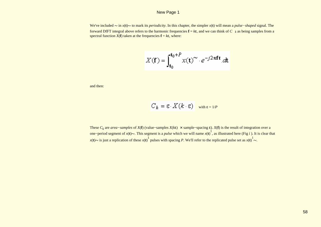
We've included ~ in x(t)~ to mark its periodicity. In this chapter, the simpler x(t) will mean a pulse−shaped signal. The

forward DfFT integral above refers to the harmonic frequencies f = kε, and we can think of Ck as being samples from aspectral function X(f) taken at the frequencies f = kε, where:

and then:

with ε = 1/P

These Ck are area−samples of X(f) (value−samples X(kε) × sample−spacing ε). X(f) is the result of integration over a

one−period segment of x(t)~. This segment is a pulse which we will name x(t)1, as illustrated here (Fig í ). It is clear that

x(t)~ is just a replication of these x(t)1 pulses with spacing P. We'll refer to the replicated pulse set as x(t)

1~.

New Page 1

58

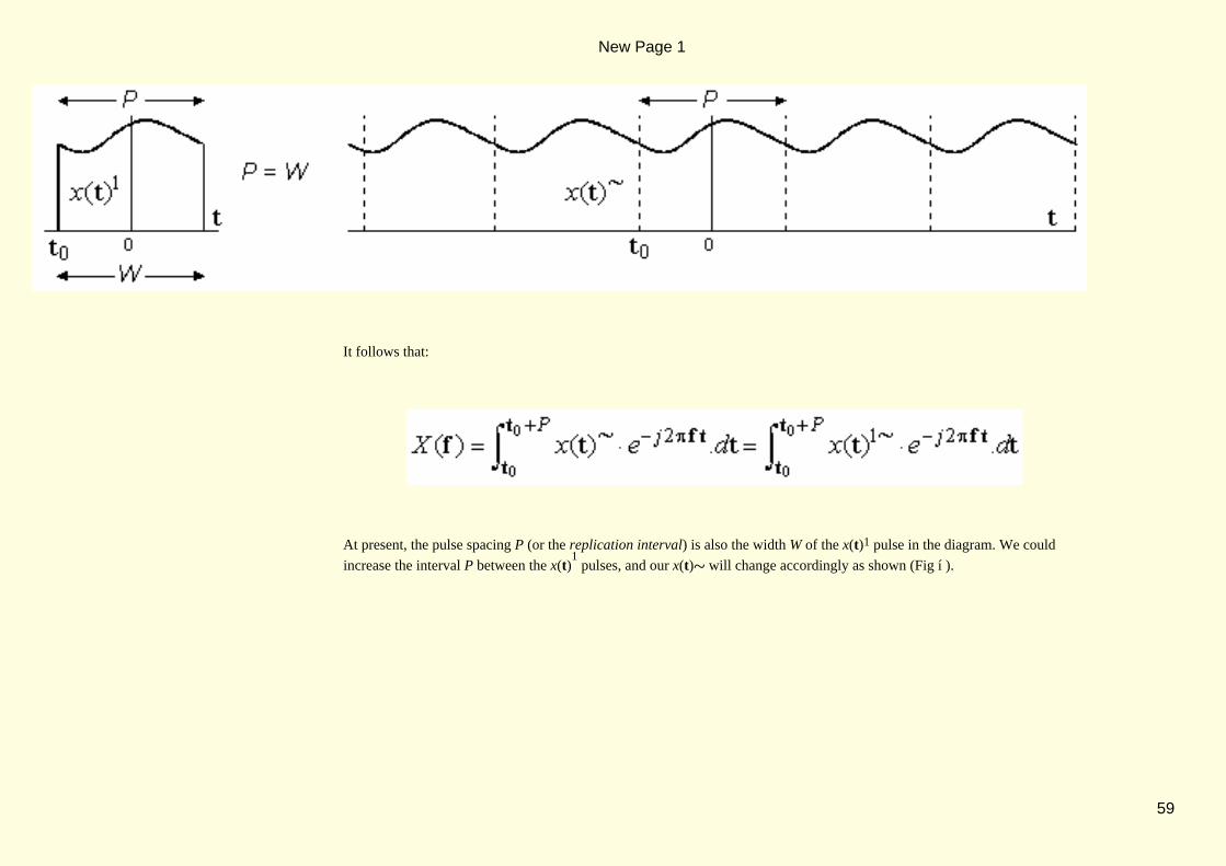
It follows that:

At present, the pulse spacing P (or the replication interval) is also the width W of the x(t)1 pulse in the diagram. We could

increase the interval P between the x(t)1 pulses, and our x(t)~ will change accordingly as shown (Fig í ).

New Page 1

59

The Ck will, of course, change also. But, we will still have the same X(f). That's because the empty space beyond the pulseadds nothing to the X(f) integral. The new Ck samples are different only because of their reduced spacing (ε = 1/P) on thesame X(f) waveform. We can carry this to the extreme by letting P → ∞, then watching what happens to Ck = ε ⋅X(kε):

The pulses move further apart and the integration range expands, while the spectral sample−spacing ε→ 0, and the samplesX(kε) crowd together into a continuum over X(f), causing f to replace kε in the limit. The central x(t)1 pulse on the t = 0 axisremains, but all of its replicas are removed to infinity, and then X(f) becomes this pulse's spectrum:

New Page 1

60

Meanwhile, the harmonics crowd ever more closely together:

As k⋅ε → f, this summation becomes an integral, and all that remains of x(t)~ is the central x(t)1 pulse:

Combining our two results:

Forward CFT Inverse CFT

This is a new transform, a Continuous Fourier Transform (CFT), and it links a pulse−shaped time signal x(t)1 to apulse−shaped spectrum X(f). The CFT is notable for its symmetry: the two integrals are almost identical, with only (−j) versus(+j) to separate the Forward from the Inverse. It might seem that the DfFT does'nt share the CFT's symmetry, but that canchange with the way we write it:

New Page 1

61

Forward DfFT Inverse DfFT

This has better symmetry, although the inverse DfFT is still numeric, it sums over a set of numbers, very different fromintegration over a function. But we can make even this sum look like an integration, if we choose to think of a number as aspecial type of pulse, which we will call an impulse. We can arrive at the impulse as an extension of this rectangular pulse(Fig ç ). As λ → 0, this pulse grows taller and narrower, but its area remains fixed at 1.0. In the limit, when λ = 0, the pulsebecomes an impulse. If we integrate across the impulse, it adds 1.0 to the area. The impulse is at once a numeric (digital) valueand an (analogue) function shape. It is our bridge between the analogue and the digital. Until now, we used a double−sidedline spectrum to describe a set of numbers. Each line represents a number, but we can also view each line as an impulse. Theline spectrum becomes an impulsive X(f) spectrum, such that an Inverse CFT integral over this X(f) becomes a sum overimpulse areas, or an ordinary numeric summation.

New Page 1

62

This diagram (Fig é ) shows how the Inverse DtFT sum over a line spectrum is the same as an Inverse CFT integral over animpulsive X(f). The impulse areas are the Ck values. They are the area−samples ε⋅X(kε) of X(f). In this way, the DfFT is justa special (impulsive) version of the CFT.

3.2.2 CFT Pairs: rectangle and sinc

A pulse in time has a pulse−shaped CFT spectrum. As an example of this, we will find the CFT spectrum of the rectanglepulse x(t) = Π(t) shown here (Fig ç ). The integration is easy:

New Page 1

63

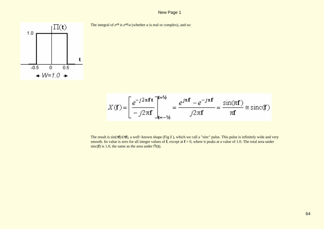
The integral of eat is eat/a (whether a is real or complex), and so:

The result is sin(πf)/(πf), a well−known shape (Fig ê ), which we call a "sinc" pulse. This pulse is infinitely wide and verysmooth. Its value is zero for all integer values of f, except at f = 0, where it peaks at a value of 1.0. The total area undersinc(f) is 1.0, the same as the area under Π(t).

New Page 1

64

The Inverse CFT integral (or ICFT) over this sinc gives a finite result (in spite of its infinite pulse width). Quite remarkably,the result will be either 0 or 1, the only possible values of Π(t). Notice how we use ↔ to symbolise a CFT pair.

From the symmetry of these waveforms, and the symmetry of the CFT/ICFT integrals, it also emerges that the CFT of a sincin time is a rectangle−shaped spectrum, that is:

To interpret this result: because the sinc−shaped time−pulse is so smooth, its spectrum is band−limited. It has no frequencieshigher than ½. These CFT pairs have great significance, and we will use them shortly.

New Page 1

65

3.3 THE DfFT AND THE DtFT

We've seen the DfFT (discrete in frequency), and we will soon find a corresponding DtFT (discrete in time). We'll developthem in a very general way, using a CFT pair x(t) ↔ X(f) as our starting point, so that the DfFT and the DtFT canboth be viewed as impulsive extensions of the CFT.

3.3.1 Sampling and Replication

We've seen how a periodic x(t)~ is fully described by its one−period pulse x(t)1, and is in fact a replication of such pulses,

that is, x(t)~ = x(t)1~. The replication interval P is also the pulse width W of x(t)

1. We also saw that x(t)

1 has a CFT

spectrum X(f).

Then we moved the x(t)1 pulses apart. The new x(t)~ is still a replication, except that P > W now. We found that the new

impulsive spectrum is still a set of area−samples Ck from the same X(f) pulse. As P increases further, the Ck samples are moreclosely spaced on X(f). Eventually, they fill all of X(f), which is now the CFT of x(t)1 (with its replicas removed to infinity).

New Page 1

66

We can understand the role of X(f) when P > W, because its pulse shape is defined by x(t)1, and that shape is preserved as

P increases. But, if we replicate x(t)1, using a spacing P < W, the pulses that form x(t)

1~ will overlap, yielding a new

periodic x(t)~ in which the shape of x(t)1 will be lost. We've illustrated this below (Fig ê ) using a triangular waveform, in

which x(t)1 is a triangular pulse, and it has a CFT spectral pulse X(f). When P = W we can say that:

When P < W, the overlapped pulse−shape is no longer triangular (Fig ê ). Over one period, this pulse is narrower thatx(t)1 and its shape is different. We've shown it as x(t)1d (Fig í ), and it must have a different CFT spectrum X(f)d.

New Page 1

67

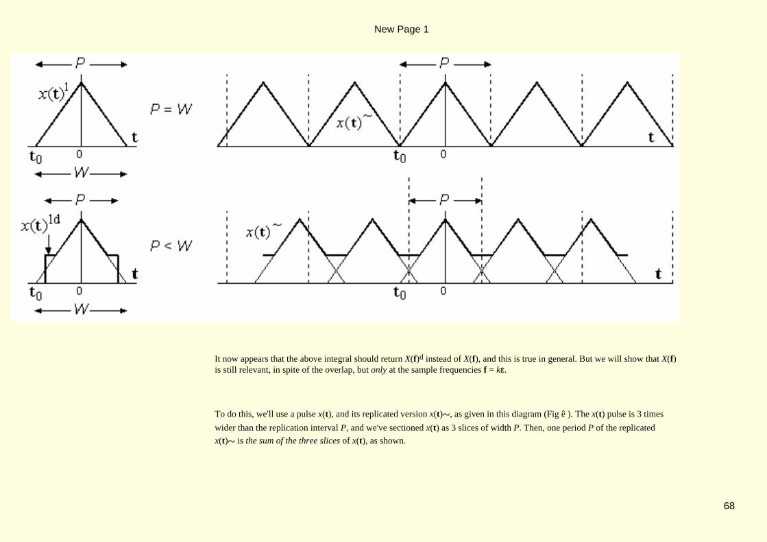
It now appears that the above integral should return X(f)d instead of X(f), and this is true in general. But we will show that X(f)is still relevant, in spite of the overlap, but only at the sample frequencies f = kε.

To do this, we'll use a pulse x(t), and its replicated version x(t)~, as given in this diagram (Fig ê ). The x(t) pulse is 3 times

wider than the replication interval P, and we've sectioned x(t) as 3 slices of width P. Then, one period P of the replicated

x(t)~ is the sum of the three slices of x(t), as shown.

New Page 1

68

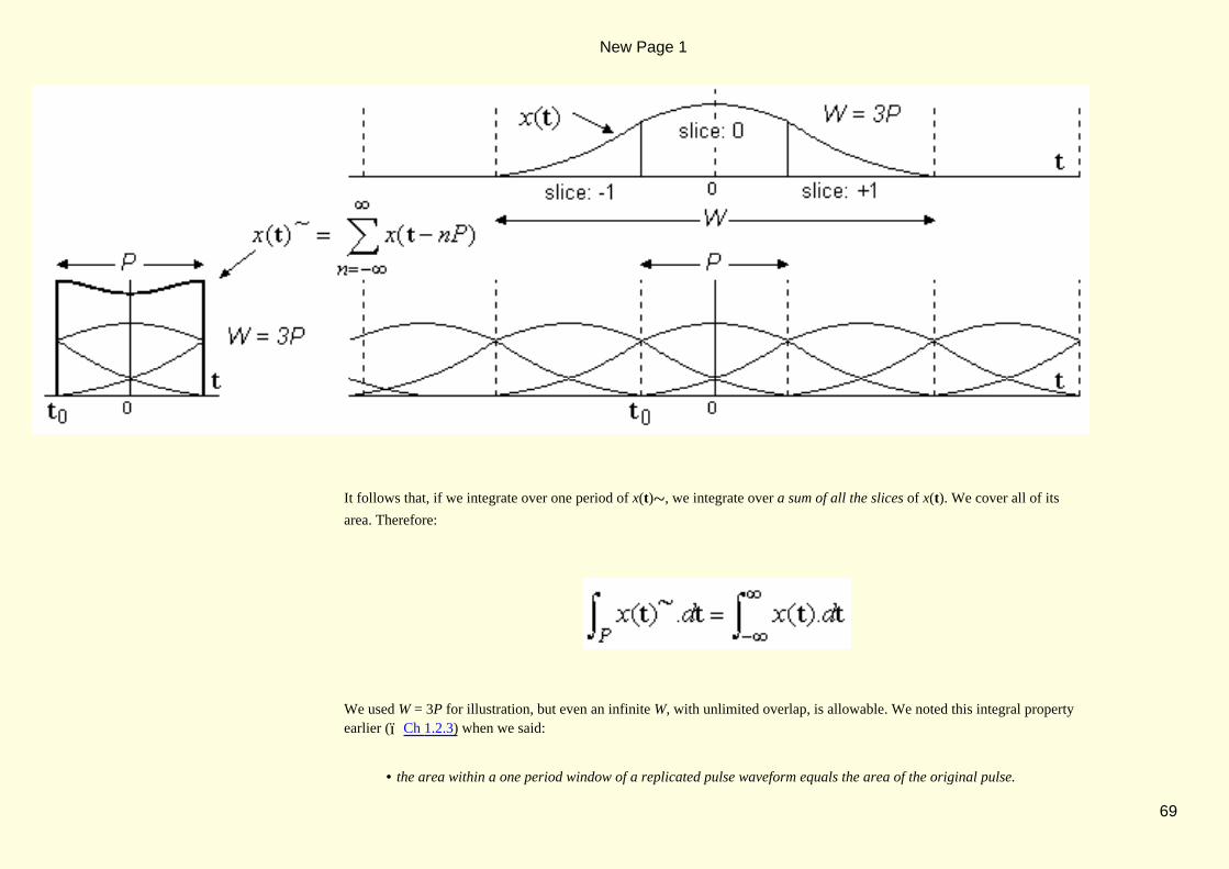
It follows that, if we integrate over one period of x(t)~, we integrate over a sum of all the slices of x(t). We cover all of its

area. Therefore:

We used W = 3P for illustration, but even an infinite W, with unlimited overlap, is allowable. We noted this integral propertyearlier (ï Ch 1.2.3) when we said:

the area within a one period window of a replicated pulse waveform equals the area of the original pulse.•

New Page 1

69

But the Fourier integral that we've encountered has an additional term, an exponent term, and when we include this term:

Note the inequality. They are not the same. To make them the same, the exponent term should look identical in each and everyslice of x(t). That calls for an exponent that is periodic in P, and this condition will be met when f = kε. We can now say that:

We have an equality again, and we can use it on our overlapped triangular waveform ( P < W ) to find that:

X(f)d and X(f) give the same result at sample points, f = kε. The picture now emerging is that if a pulse x(t) with a CFT

spectrum X(f) is replicated to form a periodic x(t)~, the FS coefficients describing x(t)~ are Ck = ε ⋅X(kε), for any replication

interval P = 1/ε, even when it causes the original x(t) pulses to overlap one another. There is another way to say this:

If a time pulse x(t) has a CFT spectrum X(f), then the DtFT spectrum of a periodic x(t)•

New Page 1

70

~, formed by replication of x(t) at intervals P = 1/ε, is a set of area−samples Ck = ε ⋅X(kε) from X(f).

Even more concicely, we could say that:

area−sampling in frequency corresponds to replication in the time domain•

We will find that the converse is also true, that we can interchange the two domains, and then we will have a DtFT as well.Now we need a more formal language to describe them both.

3.3.2 DfFT and DtFT Definitions

We will need a notation to describe number sets as impulse functions. For a solitary impulse in time, we adapt the symbol δ(t).It represents a pulse of infinite height, zero width, and unit area, occurring at time t = 0. As with any pulse, we can scale itand shift it: for example, the impulsive function 5δ(t − 4) is an impulse of area 5 occurring at time t = 4. The impulse areais also called its strength. If we multiply some continuous function x(t) by δ(t − 4) we get:

All that remains after multiplication is an impulse of strength x(4) at time t = 4. By this action we sampled x(t) at timet = 4. To sample x(t) at regular intervals of T seconds, we can define:

New Page 1

71

value−sampling

We use x(t)› to mean the value−sampled x(t). It is a string of impulses (or a set of numbers) describing value−samples x(nT)

taken from x(t). We can also define:

area−sampling

We use x(t)» to mean the area−sampled x(t). It is a string of impulses ( or a set of numbers) describing area−samples T⋅x(nT)

taken from x(t). Note, the numbers are the impulse strengths (or impulse areas), while the impulse heights are infinite.

We can define identical operations in frequency. For example, to perform area−sampling of X(f), we write:

area−sampling

After a function is sampled, only the sample values remain. Thus:

New Page 1

72

The result on the right has impulses of strength ε⋅X(kε). Values of X(f) at frequencies other than f = kε have been lost. Insimilar manner:

We also need to recall how we defined replication of x(t):

The notation that we need is now in place, and it allows us to present the CFT and the DtFT in the tabular form shown below(Fig ê ).

New Page 1

73

Row (a) of the table is for a CFT pair. The x(t) and X(f) are shown as similar bell−shaped pulses, and some pairs of this kinddo exist. They are also convenient for our illustrations. The column on the left shows the Forward and Inverse integrals (theCFT and the ICFT) that connect x(t) with X(f).

Row (b) of the table is for a DfFT pair. The diagram shows the replication of x(t) to form x(t)~, and the corresponding

area−sampling of X(f) to give us a set of impulses. We've used a special symbol to mean an area−impulse. Its drawn height isthe value X(kε), but its strength, or impulse area, is understood to be ε⋅X(kε). In this way, there is no change of scale. The sums

overhead the diagrams are just our definitions of x(t)~ and of X(f)». Notice, the spectral sample interval is ε, and the time

replication interval is 1/ε. We don't need an additional symbol P. The column on the left shows the Forward DfFT integral and

the Inverse DfFT (or IDfFT) summation that link x(t)~ to X(f)». We could say all this very compactly as:

a DfFT pair

New Page 1

74

New Page 1

75

If we look at the symmetry of the CFT and ICFT integrals, we realise that the DfFT must have a counterpart, a DtFT, withvery close similarity. We only have to swap (−j) with (+j), to interchange f and t, and to use a time−domain sample interval

T where previously we had ε, the spectral sample spacing. Whereas the DfFT linked x(t)~ to X(f)», the DtFT will link

x(t)» to X(f)~. We've presented the DtFT in row (c) of the table, and careful inspection should convince us of its validity. It

would be easy to repeat all of the arguments that gave us the DfFT, and to arrive at the DtFT instead. Now we can generaliseour earlier statement:

area−sampling in one domain corresponds to replication in the other domain•

The switch between (−j) and (+j) does not affect this conclusion. Notice in the left column of (b) and (c) above, the transformsummations run over all frequency (from k = −∞ to k = +∞), or over all time (from n = −∞ to n = +∞). As such, they arejust CFT/ICFT integrals applied to impulsive functions. But, the transform integrals in these columns run over one period only(over 1/ε or over 1/T ). In fact, there is more to be said about these, and some interesting conclusions as well.

3.3.3 Observations on Periodicity

Our triangular waveform is re−drawn here (Fig ê ), slightly modified. We've moved the one−period starting point t0 from

t = −P/2 to t = 0. That gives us a very different x(t)1 pulse (Fig í ), but when it is replicated, it gives the same x(t)~ as

before. This new x(t)1 has a different X(f) spectrum as well, but its spectral samples X(kε) have not changed, because they

describe the same x(t)~.

New Page 1

76

The same is true for any other value of t0. Every different t0 gives a different X(f) but they all share the same samples X(kε).

This lends a circular property to the periodic x(t)~ as depicted here (Fig ç ). We can place our t0 at any point and, after

P seconds, we re−visit the same values again, as if traversing a circular time path. In fact we can say this more generally:

any signal which is discrete in one domain has a circular behaviour in the other domain•

Each new t0 yields a new x(t)1 with its own unique X(f), but these are not the only X(f) pulses that share the same X(kε)samples. We can also include the X(f) spectra of all those wider x(t) pulses which overlap when replicated, but still yield the

New Page 1

77

same x(t)~ as do the x(t)1 pulses. In general, therefore, all those time pulses which replicate to form the same x(t)~ will also

share the same X(kε) values.

We can interchange the two domains, and make identical observations. The maths are much the same, but we tend to view thetwo domains differently. With this in mind, we will switch our attention to the DtFT of row (c) in the Table, and then continueour discussion from there.

3.3.4 The Sampling Theorem

The DtFT diagram is repeated here (Fig ê ), slightly altered. We've shown the X(f) pulse as band−limited, that is, it has afinite width which we will call its bandwidth, B.

New Page 1

78

X(f) is the spectrum of a time pulse x(t), and the replicated X(f)~ is the spectrum of x(t)», the area−sampled time sequence.

We chose a sample spacing of T = 1/B sec, thus ensuring that the replicated X(f) pulses would just touch one another, butwithout overlapping. This means that the identity of X(f) is not lost on replication. That would seem to imply that just the timesamples from the x(t) pulse may be sufficient to define x(t) completely, that is, even at points between the known samplepoints. We get further evidence of this if we increase the rate of sampling by making T even smaller. Then the replicas of X(f)in X(f)~ move further apart, but the X(f) pulse at f = 0 does not change. Meanwhile, the samples of x(t) grow denser and

eventually merge into a continuous x(t) which has the X(f) at t = 0 as its CFT spectrum. We can find X(f) by DtFT from a

sample set x(t)» at any spacing which does not exceed T = 1/B. ( If that limit is exceeded, spectral overlap occurs, and then

X(f) is not recoverable from X(f)~ ). Having found X(f) from samples at the maximim spacing of T = 1/B, the Inverse CFT

of X(f) can tell us all other values of x(t). It follows that:

a signal x• (t) whose double−sided spectrum is band−limited to B Hertz is fully recoverable from its samples taken at a rate exceeding Bsamples/second.

This Sampling Theorem has great importance for sampled time signals, but it is equally true that a time−pulse x(t) of finitewidth P sec has a spectrum X(f) that is fully specified by its samples taken at ε = 1/P Hertz, or less.

3.3.5 Sinc Interpolation

Given a sample set x(t)» from some x(t), the process of finding intermediate x(t) values is called interpolation. We'll first

consider a very simple x(t)» in which only one of its sample−values is non−zero. Even this has a valid interpolation, and we

already know one pulse shape that can pass through all the sample values and also fill the spaces in between. This is thetime−domain sinc, or sinc−t pulse, as shown here (Fig ê ).

New Page 1

79

An arbitrary sequence can be considerd to be a sum of one−point sequences like that shown above. This sequence (Fig ê )has five non−zero values, each of them interpolated by a sinc−t pulse of corresponding height.

The final interpolation is the sum of all the sinc pulses. It is always a smooth interpolation (Fig î ), although it can be quiteoscillatory at times.

New Page 1

80

This sum of sincs meets the time−domain constraints in that it passes through all of the given sample points. It must also meetthe frequency constraint of being band−limited to B = 1/T Hertz. To check this, we recall the CFT pair sinc(t) ↔Π(f) inwhich the zeros of sinc(t) have a spacing of 1.0, and its spectrum Π(f) has a width of 1.0. But the sinc pulses in our diagramhave a zero−spacing of T, and this changes the spectral width to 1/T, a result that matches our bandwidth constraint exactly.This argues strongly for the sinc as the true interpolator for band−limited signals. More formal methods would confirm thatthis is correct. The sinc−t interpolation yields a pulse that we call x(t)^ :

where the symbol denotes interpolation. We can conclude that x(t)^ and X(f) are a CFT pair:

Integration limits of (−∞,∞) could be used for both integrals, because X(f) is band−limited to B.

We've spoken only of a band−limited X(f), but the one−period X(f)1 pulse of a non−band−limited X(f) is by definitionband−limited, and the same result must apply to this. This gives us the result in row (d) below (Fig ê ).

New Page 1

81

New Page 1

82

Eqns (d) 1 and 2 are the CFT/ICFT integrals. We could write both with (−∞,∞) limits because X(f)1 is band−limited to 1/T.

Eqn (d) 3 refers to sample points only. In this case, any one−period width of X(f)~ will do, regardless of where it starts.

Some of the detail from the original CFT pair x(t) ↔ X(f) is no longer available in the pair x(t)^ ↔ X(f)1.

x(t)^ has only the samples from x(t), and X(f) cannot be fully recovered from X(f)1 because of spectral overlap. Both x(t)^ andX(f)1 express the same loss of information between time−samples, but they do it in different ways.

We extracted X(f)1 from X(f)~ above through multiplication by the window function Π(fT). This Π(fT) equals 1.0 for

(−½/T < f < ½/T ) and is zero everywhere else. Windowing is a widely−used concept in DSP.

When we interchange the domain roles, row (e) gives us the results for DfFT interpolation. Eqns (e) 1 and 2 are the CFT/ICFTintegrals. We could write both with (−∞,∞) limits because x(t)1 is band−limited to 1/ε. Eqn (e) 3 refers to sample points only.

In this case, any one−period width of x(t)~ will do, regardless of where it starts.

In the next section, we will sample the band−limited pulses x(t)1 and X(f)1 and this will replicate their interpolated spectra.This process will bring us to the Discrete Fourier Transform (DFT), a transform which is discrete in both domains.

New Page 1

83

3.4 THE DFT

The DFT has importance as the all−numeric transform for computer use. We will derive it now, but we will defer all use of theDFT until later.

3.4.1 From Interpolated DfFT and DtFT to the DFT

Starting from the CFT pairs:

x(t) 1

↔ X(f)^ and x(t) ^ ↔ X(f)1

we will area−sample the band−limited x(t)1 and X(f)1 pulses at a spacing which equals the band−width divided by N, whereN is any positive integer. This has the effect of replicating X(f)^ and x(t) at a spacing which is 1/(band−width). Theseoperations give us the signals shown here (Fig ê ).

New Page 1

84

New Page 1

85

In row (f), we had sampled X(f) with sample spacing ε. This gave a bandwidth of 1/ε for x(t)1 and the sample−spacing in timebecomes 1/Nε as shown. This time−sampling causes X(f)^ to be replicated at intervals of Nε to yield a new periodic signal

[X(f)^]~. When the replicas are added, the sample points of all the replicas in [X(f)^]~ will be alligned, but only because we

chose N as an integer. Thanks to this allignment, and because the samples of X(f)^ are also samples of X(f), the samples of

[X(f)^]~ will now become samples of X(f)~. This allows us to write a forward CFT over the area−samples of x(t)1 , but we

will evaluate it only at the points f = kε.

The signal [x(t)1]» is a set of area−impulses, and the integration reduces to a summation over time−samples at spacing

of 1/Nε. It becomes:

We can make a corresponding statement about the signals in row (g):

New Page 1

86

The signals in row (f) have two spacing parameters, N and ε, while the signals in row (g) have spacing parameters N and T.There is no necessary relationship between ε and T, but, if we choose T and ε such that:

1/Nε = T or, equivalently, 1/NT = ε

we will have the same sample positions (in time and in frequency) for row (e) that we have for row (f). Then both rows willrefer to the same numeric data and we can re−write our summations as:

Forward DFT

and

New Page 1

87

Inverse DFT

The diagram shows summing ranges for n and k to cover one period with N = 8. But the range −4 .. +3 can be replaced bythe range 0 .. 7 without penalty. In fact, any set of N consecutive samples will do, and the range 0 .. N−1 is widely used asa matter of convenience.

These equations apply to the replicated signals x(t)~, X(f) ~, but not to the original CFT pair x(t), X(f). They connect

N time−samples that span one period of x(t)~ to N spectral samples that span one period of X(f)~. They use a sum over

area−samples in one domain to determine value−samples in the other domain. On a purely numeric level, the DFT uses anN−point time vector x[n] to find an N−point spectral vector X[k], and the Inverse DFT (or IDFT) uses X[k] to restore theoriginal x[n].

The use of replicated signals x(t)~, X(f) ~ rather than x(t), X(f) is a necessary consequence of sampling, because

replication in one domain is an expression of what was lost between samples in the other domain. For a fully digital transform,replication in both domains is inevitable.

But overlap is not inevitable. For a given CFT pair x(t), X(f), it is possible for x(t) or X(f), but not both, to be band−limited.Thus, in one domain only, we can have replication without overlap. This can mean that x(t)1 = x(t), or that X(f) 1 = X(f), butnot both of these simultaneously.

This concludes our introduction to Fourier Transform theory. We now have the transform base that we need for the DFTapplication work of later chapters.

New Page 1

88

New Page 1

89

4.1 PREAMBLE

The DfFT, also known as Fourier Series, provides discrete spectral descriptions of periodic time signals. Periodic signals areimportant in several areas of engineering, and their spectra are frequently of interest. This chapter takes a closer look atFourier Series.

New Page 1

90

4.2 PERIODIC WAVEFORMS AND THEIR PROPERTIES

We will examine a number of periodic waveforms, with observations about their symmetry, and the spectral implications. Wewill see the spectral impact of time−shifting a signal. We will show the Energy and Power expressions for these signals. Wewill look at periodic impulse trains with their periodic impulsive spectra. Finally, we will talk about Harmonic Distortion,which is a useful measure of non−linear effects in amplifiers and related equipment.

4.2.1 The Rectangular Waveform

The rectangular waveform (Fig ê ) is a replication of rectangular pulses, each of width W, and with pulse spacing P > W.

New Page 1

91

We can start by taking the CFT of the pulse, which we will call x(t):

Finally:

We can then specify the FS coefficients as:

From these, we can re−construct the periodic waveform as:

New Page 1

92

A direct summation that used A = 1, P = 1 and W = 0.25, up as far as k = 10 (the tenth harmonic) gave this result(Fig ê ).

We can see an oscillation (often called "Gibb's oscillation") that is widely observed in Fourier synthesis. It occurs when weattempt sharp transitions with a limited bandwidth (frequencies no higher than 10/P or 10 Hz in this case). If we include moreharmonics, the frequency of the oscillation will increase but its amplitude will not diminish. Later on, we'll describe ways tocurb the oscillation where needed. If this waveform looks familiar, its because we saw it before (ï Ch 2.3). On that occasionthe Ck expression seemed quite different, and this brings us to our next topic.

4.2.2 Time−shifted Waveforms

New Page 1

93

The present x(t)~ has its t = 0 axis on the centre of a pulse, and this imparts even symmetry to the waveform. The Ck that we

found for it are real−valued numbers. This means that argCk = 0, causing x(t) ~ to be built from a sum of pure cosines.

That makes sense, because the cosines themselves have even symmetry also.

Our earlier x(t)~ (ï Ch 2.3) had its t = 0 axis on a pulse edge, equivalent to a right−shift (a delay) of the present waveform

by τ = W/2 sec. We also noted (ï Ch 2.2.3) that a τ sec delay was equivalent to a phase change of −2πf1τ radians at somefrequency f1. To apply this phase change to our Ck coefficients, where the harmonic frequencies are (kε) Hertz, we require:

We will apply this to the waveform that we just plotted:

Compare this with our earlier result:

They may not look the same, but they are the same. That's easily checked numerically, but can you manipulate the equationsto prove it ?

New Page 1

94

We've just shown how a signal's spectrum changes when the signal is shifted in time. A shift of τ seconds multiplies thespectrum X(f) by e−j2πfτ . This multiplier has a magnitude of 1.0. We conclude that:

time shifting of a signal does not alter the spectral magnitude, but it applies a linear−phase adjustment to the phase.•

This result holds for all periodic waveforms, and equally for other waveforms, so we will meet it quite a lot in the future.

4.2.3 Periodic Waveform Listing

We've tabulated several waveforms here (Fig ê ).

New Page 1

95

New Page 1

96

For the Rectangular waveform, we used the Forward CFT integral of the one−period pulse to arrive at the X(f) formula. Thesame approach, with a little more algebra, gives us the others X(f) expressions in the Table. If the Triangle waveform were tobe constructed using W < P, we would see the change of shape, due to overlap, that we predicted earlier (ï Ch 3.3.1).

The Rectangle, Triangle and Half−Cosine all have even symmetry about t = 0. They also have real−valued X(f) expressions,and the Ck values, which are samples from X(f), will be real−valued too. This is as it should be, because waveforms with evensymmetry are constructed from cosines, and cosines have zero phase.

A waveform which has odd symmetry about t = 0 is built from sines rather than cosines, because the sines themselves haveodd symmetry. In this case, the Ck values will have phase−angles of ±π/2. As such, they are imaginary numbers. The Rampand Sign waveforms have odd symmetry, and their X(f) expressions are imaginary as anticipated.

It makes sense to avail of waveform symmetry wherever possible. If we shift a symmetric waveform horizontally, we destroythat symmetry, and the coefficients Ck become complex (rather than just real or imaginary). However, they do so in a verypredictable way, by application of a linear phase lag, as was demonstrated earlier. To recap, if we modify any of these X(f)according to:

applying a τ−second delay

the x(t)~ reconstruction is moved horizontally by τ seconds, to the right (a time delay) when τ is positive, and to the left (a

time advance) when τ is negative.

4.2.4 Odd Half−wave Symmetry

New Page 1

97

The Fourier Series coefficients of a periodic x(t)~ can be found from:

A waveform having odd half−wave symmetry is one for which:

Here (Fig ç ) we see one period from different waveforms, and waveform (a) has odd half−wave symmetry. For evenharmonics (when k is a multiple of 2), the exponent term in the range (0 < t < ½P) is repeated exactly in the range

(½P < t < P), while the x(t) ~ shape just changes sign. The two halves of the Ck integral will have equal and opposite areas.

It follows that Ck = 0 when k is even, and that odd half−wave symmetry causes the even harmonics to disappear altogether.

Waveform (b) might seem more symmetric, but it does not have odd half−wave symmetry. Waveform (c) is a special case ofwaveform (a), so it too has no even harmonics. The same can be said of waveform (d). Waveforms like this can occur as thedistorted responses to sine−wave inputs in balanced amplifier circuits, and the absence of even harmonics is well known inthis context.

Some of the waveforms that we tabulated have no even harmonics under certain conditions. The Sign waveform has no DClevel, and it has no even harmonics when W = P. The Triangle waveform has no even harmonics when W = P, but it does havea DC level of A/2.

New Page 1

98

4.2.5 Power and Energy

As a matter of definition, the mean power px of a periodic x(t)~ is the Energy over a period P, divided by P, that is:

New Page 1

99

In general, x(t)~ is built from sine waves of amplitude Mk = 2|C

k|, each with a mean power of ½M

k

2, which is 2C

k

2. Each of

the two phasors that make up the sine wave contributes half of this power, that's a mean power of |Ck|2 for each phasor. Itfollows that:

We've used a modulus symbol | | on both expressions to mean the magnitude, or the vector length. We must do that for

complex numbers (such as Ck ), but its use is optional for real signals (such as a real−valued x(t)~ ).

The integral over one period of x(t)~ is an integral over the x(t)1 pulse which has a finite width P. The Energy of this pulse

(noting that Ck = εX(kε) ) is:

New Page 1

100

This refers to the CFT pair x(t)1 ↔ X(f)^ , and the X(kε) are samples from X(f). For an arbitrary pair x(t) ↔ X(f) , we could not express the energy in terms of samples from X(f), but we can do so here becausex(t)1 has finite width P and can be represented by its spectral samples, taken at a spacing of 1/P or less.

Notice, the summation describing Ex is the approximate area under [X(f)^]2. In this case, because x(t)1 has finite width P, it is

also the true area under [X(f)^]2. This is a consequence of sinc interpolation, using some properties of the sinc pulse which wewill now briefly introduce.

4.2.6 Properties of the Sinc Pulse

We defined the sinc pulse to be:

and its main characteristics are shown here (Fig ê ). It is a smooth pulse which, for integer n, satisfies sinc(n) = 0, but withthe exception that sinc(0) = 1.

New Page 1

101

The distance between zero−values is the lobe width, which is 1.0. The shaded area above is called the main lobe, but it is twolobes wide and its area is about 1.18. The sinc has some notable properties under integration. Firstly, the total sinc area isexactly 1.0, that is:

sinc area is 1.0

Secondly, for integer values of m and n :

This is the orthogonality property of overlapping sinc pulses. Except when they coincide, they interact destructively, and theirproduct area is zero. The sincs coincide when m = n, and if we set m = n = 0, we obtain:

New Page 1

102

sinc

2

area is 1.0

This sinc−squared pulse is always positive, as shown here (Fig ê ).

With these results, we can comment on the area under sinc−interpolated data sets.

New Page 1

103

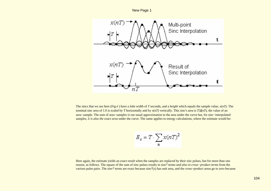
The sincs that we see here (Fig é ) have a lobe width of T seconds, and a height which equals the sample value, x(nT). Thenominal sinc area of 1.0 is scaled by T horizontally and by x(nT) vertically. This sinc's area is T⋅x(nT), the value of anarea−sample. The sum of area−samples is our usual approximation to the area under the curve but, for sinc−interpolatedsamples, it is also the exact area under the curve. The same applies to energy calculations, where the estimate would be:

Here again, the estimate yields an exact result when the samples are replaced by their sinc pulses, but for more than onereason, as follows. The square of the sum of sinc pulses results in sinc2 terms and also in cross−product terms from thevarious pulse pairs. The sinc2 terms are exact because sinc2(x) has unit area, and the cross−product areas go to zero because

New Page 1

104

sinc(x − n) ⋅sinc(x − m) integrates to zero when n ≠ m. A little earlier (ï Ch 4.2.5), we wrote the energy of a band−limitedtime pulse as a sum over spectral samples:

Here too, the sum gave an exact result, identical to the area under |X(f)|2, because the X(f) of a band−limited time signal isrelated to its samples by sinc interpolation.

New Page 1

105

4.3 IMPULSIVE WAVEFORMS

Here we derive some impulsive periodic transform pairs. They are comprised of impulse trains in both domains. Their mainsignificance is as the theoretical sampling functions that convert analogue signals into sampeld−data sequences.

4.3.1 Railings Transform Pairs

We now return to the rectangular pulse train, but with a few minor changes included (Fig ê ). We've set the pulse height A tobe 1/W, and we've re−defined the pulse spacing with symbol T rather than P.

New Page 1

106

With these changes, AW = 1, and then X(f) = sinc(Wf). The Ck values are its area−samples, and if we define λ = 1/T weget:

The result becomes more interesting if we let W→ 0. Then each pulse becomes tall and narrow, and eventually becomes aunit−area impulse when W = 0. We then have a string of impulses of strength 1.0 with spacing T, and their spectrum is:

All coefficients now have the same value, λ. This Ck spectrum is a sequence of numbers, but we can treat each number as animpulse, with impulse strength (or area) as given by the numeric value. The result is a highly unusual transform pair thatlooks like this (Fig ê ) :

New Page 1

107

Both sides are impulse trains, with reciprocal spacing, T and 1/T, ( or 1/λ and λ if we prefer). By adapting two differentimpulse symbols, we can conveniently have the same drawn height of 1.0 on both sides. On the left, we have value−impulses,of strength equal to drawn height. On the right, we have area−impulses, of strength equal to (drawn height

× impulse−spacing). The left side is called a value−sampler. The right side is called an area−sampler. They are sometimescalled "Railings" because of their resemblance to a railing−type fence.

We obtained this from a pulse train with a pulse height A = 1/W, which gave a pulse area of 1.0, and this became the impulsestrength on the left−hand side. If we had set A = T/W instead, the left−side impulse strength would be T, and the right−sideCk coefficients would be larger by T, with a value of 1.0. This gives us an alternative rendering of the same transform pair, asshown here (Fig ê ).

New Page 1

108

Notice how the value−sampler and the area−sampler have changed places. If a continuous signal x(t) were to be multiplied bythe area−sampler on the left, the result would be a set of impulses with spacing T and with impulse strengths T⋅x(nT). Innumeric form, this is just a set of area−samples from x(t), which is the reason that we called this an area−sampler. By the samereasoning, we could multiply x(t) by a value−sampler to get a set of value samples x(nT). We can summarise our findings bysaying:

an area−sampler transforms to a value sampler• a value−sampler transforms to an area−sampler•

These are rather extreme tramsform pairs. To give some appreciation of how they work, we will sum the harmonics of themost recent pair, in an attempt to build the area−sampler on the left. The right side says that Ck = 1 for all k, and so:

New Page 1

109

This reduces to a DC level of 1.0 plus a sum of cosines:

To see how this x(t)~ develops, we summed as far as k = 8, and got the result shown here (Fig ç ). In the limit, we expect a

set of impulses, each of area T. This result is tending that way, with a pulse area of about (17 × T/17) on inspection. Atmultiples of T, the cosines are in phase and they add up. At all other times they are out of phase, and ultimately sum to zero. Inthis way, we can account for these Railings transform pairs.

Later on, we may find these pairs of some assistance, in that they can help us to visualise the consequences of sampling.

New Page 1

110

4.4 HARMONIC ANALYSIS

One of the practical uses for Fourier Series is in the measurement of how a sine wave is distorted by its transmission throughan amplifier, or through some other analogue system. Because of system non−linearities, there is some distortion of the signalshape at the output. It is no longer a pure sine wave, but its frequency has not changed. The distortions will be seen as smallharmonic components of the sine−wave frequency. We use the amplitude of these harmonics as a measure of the distortionintroduced by the system.

4.4.1 Measuring Harmonic Distortion

On this plot (Fig ç ), the dotted line is a straight line at 45° describing the input−output relationship of an ideal unity−gainamplifier. The solid line is closer to reality. It saturates at the highest output levels, and shows some non−linearity within thesignal range. A sinusoidal vin will emerge somewhat distorted as vout. A spectral analysis of vout will show up some harmoniccomponents. The amplitude of these harmonics is a useful measure of the distortion.

The signal vout is the sum of its harmonic components :

New Page 1

111

where v1(t) is the fundamental, v2(t) is the 2nd harmonic, etc. The distortion is from the sum of the harmonics, withinstantaneous distortion power:

We want only the mean power over a cycle, and we will find that the mean of the cross−product terms like 2v2(t)v3(t) is zero.(That's because the different harmonics are uncorrelated with one another). Consequently

New Page 1

112

where the bar overhead indicates mean value. We typically define the harmonic voltages to be the square−roots of thesemean−power terms:

and the total harmonic distortion, or THD, in per−cent, becomes:

where V1 is the rms value of the fundamental. Notice however that we can use peak sine−wave values to get the same result,because all of these waveforms share the same sinusoidal shape.

The distortion due to one harmonic component may be of special interest. For example, we can write the distortion due to thesecond harmonic component as:

New Page 1

113

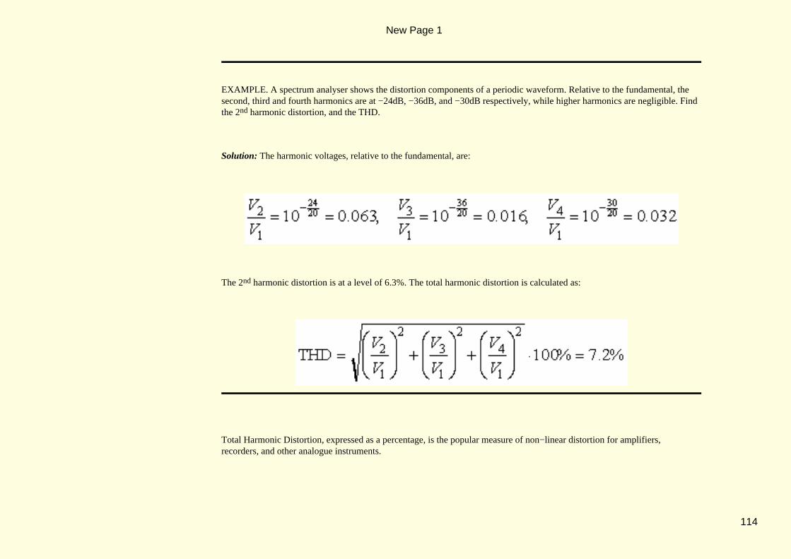
EXAMPLE. A spectrum analyser shows the distortion components of a periodic waveform. Relative to the fundamental, thesecond, third and fourth harmonics are at −24dB, −36dB, and −30dB respectively, while higher harmonics are negligible. Findthe 2nd harmonic distortion, and the THD.

Solution: The harmonic voltages, relative to the fundamental, are:

The 2nd harmonic distortion is at a level of 6.3%. The total harmonic distortion is calculated as:

Total Harmonic Distortion, expressed as a percentage, is the popular measure of non−linear distortion for amplifiers,recorders, and other analogue instruments.

New Page 1

114

New Page 1

115

5.1 PREAMBLE

A signal, after sampling, becomes a data sequence, and we will look at the effects of sampling of a periodic signal. The rate ofsampling must be high enough to avoid aliasing, a phenomenon that we will investigate. From the sampling of periodicsignals, we will see how spectral replication brings us once again to the DFT, but by a different route from before, and withsome helpful new insights to be added. Although we've seen the DFT before now, this chapter brings it much closer from anapplications perspective.

New Page 1

116

5.2 SINE−WAVE SAMPLING AND IMAGING RULES

If we sample a signal frequently, such that it changes only slightly between samples, then the samples will give a goodimpression of the underlying shape. Less frequent sampling (larger T) gives a poorer result, with substantial signal variationsbetween samples. It would appear that the signal values between samples are lost forever, but the sampling theorem which wediscussed (ï Ch 3.3.4) assures us that this is not necessarily so :

a signal x• (t) whose double−sided spectrum is band−limited to B Hertz is fully recoverable from its samples taken at a rate exceeding Bsamples/second.

To meet the band−limited condition, the spectrum X(f) that describes x(t) must go to zero for |f| > ½B, (Fig ç ). We canthen use a sampling rate fS as low as fS = B = 2f max, where fmax is the highest signal frequency in x(t). This rate ofsampling gives us only two samples per cycle at fmax . We're assured that this very sparse sampling is sufficient for accuratereconstruction. We'll need some time to appreciate this fully, but we can start the process now by looking at some sampledsinusoidal waveforms.

New Page 1

117

5.2.1 Sampled Phasors and Sampling Ambiguity

Suppose we take a sine wave of frequency f and initial angle α.

Then we sample it at a rate of fS = 1/T samples/sec :

This result depends only on the ratio (f/fS), a normalised measure of frequency, to which we will assign the symbol f :

cycles per sample−interval (normalised freq)

Then:

New Page 1

118

With this step, we've moved from f and t to a normalised f and to an integer time parameter n, which is time expressed as asample count. This is a routine transition when we perform Analog to Digital (A/D) conversion on a signal:

(cycles/sec) × secs (cycles/sample) × samples

It establishes a new time scale, in which the sample−interval replaces the second as "one unit of time". Once a signal issampled, its best to use f rather than f because it allows us to process the data independently of the actual rate of sampling.We now think of the signal frequency f as cycles per sample interval and, according to the sampling theorem, it can be ashigh as 0.5, (equivalent to 0.5 × fS samples/sec) but not any higher. The range of signal frequencies becomes (0 < f < 0.5)for a single−sided spectral view, or (−0.5 < f < 0.5) for a two−sided spectral view.

We can show rather simply why these limits must apply. We begin by expressing x[n] as a sum of two phasor terms, just as wedid earlier (ï Ch 2.2.3) for a continuous sinusoidal x(t) :

But these are sampled phasors, and we can view the anti−clockwise (+ f ) phasor and the clockwise (− f ) phasor atsuccessive sample positions as they rotate (Fig ç ). We should recognise f as the angle between successive samples,expressed as a fraction of a cycle. The drawn angle here (Fig ç ) is 45°, and it describes a frequency of f = 1/8 cycles/sample = 0.125. Also shown is the initial angle α when n = 0, drawn as 60° on the diagram. The (+ f )phasor starts at +α, while the (− f ) phasor starts at −α. The sum of the two phasors at any instant is a real number, and ittraces out the sampled sinusoid, x[n]. The x[n] that these phasors describe are shown here (Fig í ).

New Page 1

119

We now consider what happens if we take the signal frequency f above, and far beyond, the limit of 0.5 fS. This will take f far beyond 0.5. At f = 0.5, there is 180° between samples. At higher frequencies, a confusion sets in, as follows.

Our drawing showed the (+ f) phasor at f = 0.125, (Fig ë ), or 1/8 cycle between samples. We could not distinguish thisresult from f = 1.125, which includes an extra (unseen) cycle between samples. The same is true for f = 2.125, and for f = 3.125, and so forth.

New Page 1

120

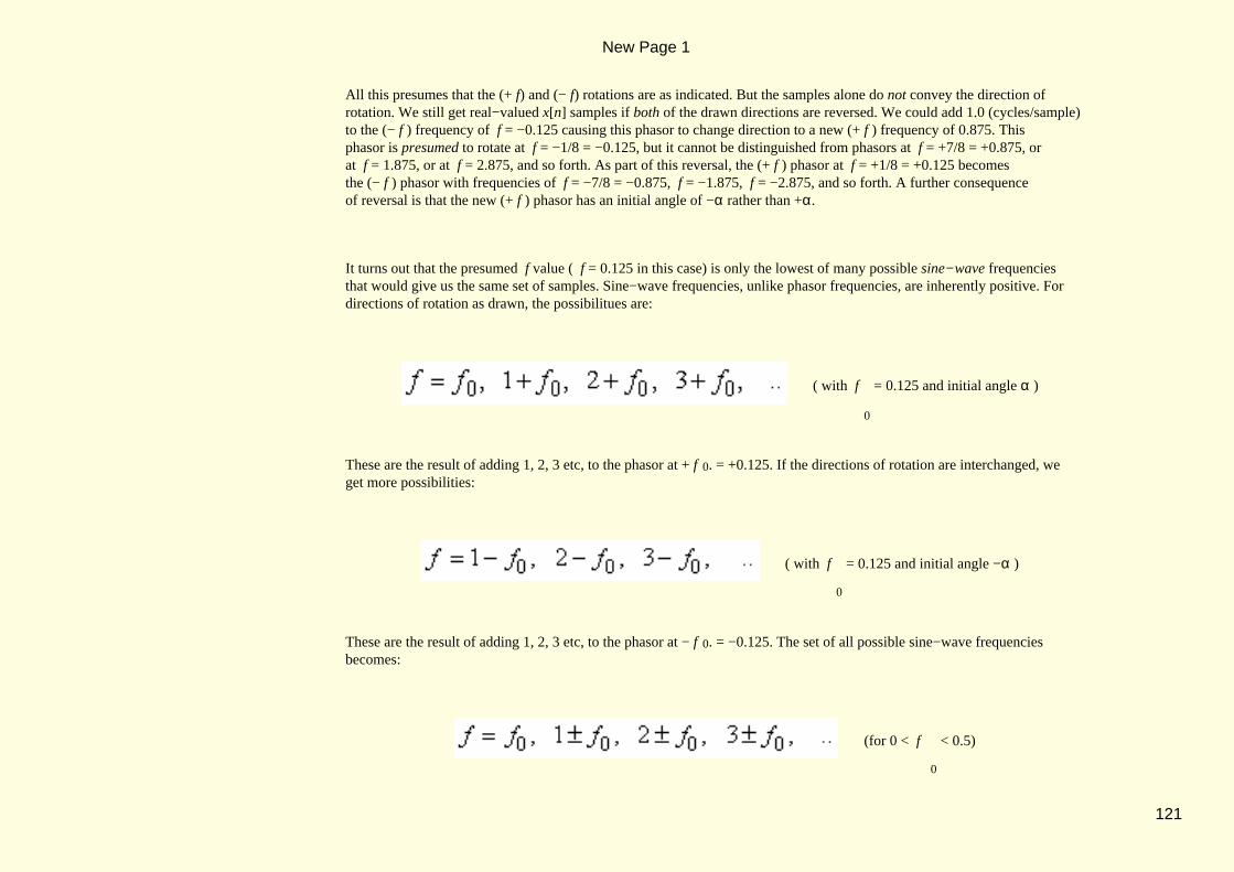
All this presumes that the (+ f) and (− f) rotations are as indicated. But the samples alone do not convey the direction ofrotation. We still get real−valued x[n] samples if both of the drawn directions are reversed. We could add 1.0 (cycles/sample)to the (− f ) frequency of f = −0.125 causing this phasor to change direction to a new (+ f ) frequency of 0.875. Thisphasor is presumed to rotate at f = −1/8 = −0.125, but it cannot be distinguished from phasors at f = +7/8 = +0.875, orat f = 1.875, or at f = 2.875, and so forth. As part of this reversal, the (+ f ) phasor at f = +1/8 = +0.125 becomesthe (− f ) phasor with frequencies of f = −7/8 = −0.875, f = −1.875, f = −2.875, and so forth. A further consequenceof reversal is that the new (+ f ) phasor has an initial angle of −α rather than +α.

It turns out that the presumed f value ( f = 0.125 in this case) is only the lowest of many possible sine−wave frequenciesthat would give us the same set of samples. Sine−wave frequencies, unlike phasor frequencies, are inherently positive. Fordirections of rotation as drawn, the possibilitues are:

( with f

0

= 0.125 and initial angle α )

These are the result of adding 1, 2, 3 etc, to the phasor at + f0. = +0.125. If the directions of rotation are interchanged, weget more possibilities:

( with f

0

= 0.125 and initial angle −α )

These are the result of adding 1, 2, 3 etc, to the phasor at − f0. = −0.125. The set of all possible sine−wave frequenciesbecomes:

(for 0 < f

0

< 0.5)

New Page 1

121

The eligible frequencies above f0 are called the images of f0. The actual frequencies in samples/sec (or Hertz) are just these f values multiplied by fS. If a signal x(t) could contain more than one of these frequencies, then its samples x(nT) cannotdistinguish one from another. From the samples alone, there is no way to say from which of the images they originated. Thesamples describe the sum of image components, and there is no way to separate them. This describes the ambiguity thatsurrounds a signal after sampling. The only way to avoid it is to guarantee, in advance, that x(t) can contain only one (usuallythe lowest) of a whole set of image frequencies. In other words, x(t) must be band−limited, and the limits are the same as waspredicted by the Sampling Theorem. This brings us to the subject of image bands.

5.2.2 Normalised Frequency and Image Bands

This spectral diagram (Fig ê ) shows the various images that we described. Each line describes a phasor with a (fractional)frequency label attached. The phasors at (±1/8) describe the f0 sinusoid. The phasors at (±7/8) are for the (1− f0) sinusoid.The phasors at (±9/8) are for the (1+ f0) sinusoid. This pattern is repeated at higher frequencies. Notice, the black (+1/8)phasor is replicated up and down the spectrum with a spacing of 1.0 on the f scale. The gray (−1/8) phasor is replicated in anidentical manner. Taken together, the (black + gray) phasor pair at (±1/8) is replicated at intervals of 1.0 to form a periodicspectrum. This concurs with our earlier finding that sampling in time equates to spectral replication (ï Ch 3.3.2).

New Page 1

122

The dotted frames on the diagram are a set of one−period windows, each of width 1.0, and each divided in two by a verticalline at the centre. This divides the spectrum into numbered bands, with the band numbers overhead, such that each bandcontains one of the possible frequencies. The range (−0.5 < f < +0.5) is band−0, usually called the base−band, withhalf−bands labels (0−, 0+) overhead. The ranges (−1.0 < f < −0.5) and (+0.5 < f < +1.0) define band−1 withhalf−band labels (1−, 1+) overhead. Similarly for band−2, with labels (2−, 2+) overhead. When a base−band sinusoid x0(t)of frequency f = f S/8 is sampled at rate fS, the samples can be interpreted as base−band phasors at f = ±0.125, or asband−1 phasors at f = ±0.875, or as band−2 phasors at f = ±1.125, and so forth. Thus, any of several analogue signalscould have given us the same set of samples :

the band−0 interpretation

the band−1 interpretation

the band−2 interpretation

Notice how the initial angle changes sign in the odd−numbered bands. If we have only the samples to work with, they couldhave come from any of these analogue signals. These signals, with one signal per band, are just some of the possible"interpretations" of a single set of samples. We can easily confirm this by substituting t = nT in x0(t), x1(t) and x2(t) to findthat x0(nT), x1(nT) and x2(nT) are identical sets of data values.

From a set of image frequencies f0, 1±f 0, 2±f 0, 3±f 0, etc , it is usually the base−band frequency f0 that is theintended frequency. To protect this signal from the corrupting effect of images, we must guarantee that the higher imagefrequencies do not exist in the signal, or are reduced to an acceptable level. To do this, the analogue x(t) must be filtered inadvance by an analogue low−pass filter so as to remove those parts of x(t) at frequencies higher than ½fS. In this way, x(t)becomes band−limited to the base−band region. Because image frequencies are sometimes called "aliases", the analogue filterthat does this is called an anti−alias filter. We'll have more to say about these in due course.

New Page 1

123

New Page 1

124

5.3 PERIODIC SIGNAL SAMPLING AND THE DFT

Now that we know the imaging rules, we will apply them to periodic signals, so as to determine the consequences of sampling.We will see how these efforts lead us directly to the Discrete Fourier Transform (DFT).

5.3.1 Aliased FS Coefficients

This is the spectral plot (Fig ê ) of a periodic signal x(t)~. The heavy black lines are the FS coefficients Ck , with

line−spacing ε = 1/P the reciprocal of the waveform period.

The harmonics imply periodicity, but do not account for the band−structure that we've superimposed. These bands describe aproposed sampling of this signal at a rate fS = Nε, with N = 9 on the diagram. The window width is fS, which is also 1/T,where T is the sample−interval. We've also shown the normalised frequency scale. In terms of f, the harmonics now occur at1/N, 2/N, 3/N, etc, reaching N/N = 1.0 at the sampling frequency.

New Page 1

125

The spectral lines describe coefficients Ck before x(t)~ is sampled. When we sample x(t)~, the spectrum is replicated. The

entire set of lines is duplicated at intervals of fS, or at intervals of 1.0 on the f scale. The result is shown here (Fig ê ). Thefinal set of lines is the sum of all the replicated sets.

New Page 1

126

This final set is periodic as shown. Notice, all of the lines fall into harmonic positions because fS = Nε, with integer N. IfN were not an integer, a much more difficult and complex picture would emerge, and we don't want to deal with that just yet.The result is a new set of coefficients Ck' such that:

We've shown just a few terms of an infinite set. A more compact description would be:

New Page 1

127

Because there are N harmonics in a spectral window, the new set Ck' must be periodic, with a period of N = 9. It means thatCk' has only N unique values, occupying one spectral window, and the same values are repeated in each and every window.

The action of sampling with N = 9 generates N samples over precisely one period of x(t)~. We then have N unique sample

values and, because N is an integer, the same set of N samples occur for all other periods of x(t)~. If N were not an integer, the

sample set from x(t)~ would not be periodic in N. It might be periodic over some higher number of samples, or, it might not

be periodic at all !

With N = 9, we have 9 unique time samples described by 9 unique Ck' values. It makes sense that a sampling action whichreduces the data to a mere 9 samples in time should have a corresponding effect in frequency, giving us 9 spectral coefficientsas well. More generally, this is a transform mechanism that links a set of N time samples to a set of N spectral coefficients. Itis a Discrete Fourier Transform, or a DFT.

5.3.2 The Discrete Fourier Transform (DFT) −− Again

We've already arrived at the DFT, but by a different route (ï Ch 3.4), and with some difference in notation, as follows:

New Page 1

128

Forward DFT

and

Inverse DFT

with: 1/Nε = T or, equivalently, 1/NT = ε.

The indexes n and k normally use the range 0 .. N−1, but a range such as m .. m+N−1 (where m is any integer), will dojust as well. Both of these DFT expressions perform a sum over area−samples to deliver a set of value−samples, and both

refer to periodic signals x(t)~ and X(f)~ which can (optionally) be considerd to be the replicated versions of pulses x(t) and

X(f). In our Fourier Series discussion, the Ck were the area−samples ε⋅X(kε) from X(f). By observing that

N⋅Ck' = N ⋅ε⋅X(kε)~ = X(kε)~/T, we can re−write the DFT and the IDFT in terms that use C

k' as the spectral quantity:

Mathcad CFFT

New Page 1

129

Mathcad ICFFT

CFFT and ICFFT are the function names in Mathcad that perform these DFT operations, but they do so using a "fast"computational algorithm. The label CFFT means "Complex Fast Fourier Transform", and ICFFT is its Inverse. The MATLABdefinitions, however, are in terms of NCk' rather than Ck' :

Mathcad N⋅CFFT, MATLAB fft

Mathcad ICFFT/N , MATLAB ifft

The MATLAB functions are called fft and ifft, again using a fast algorithm. The Ck' notation is fine for Fourier Series work,but a popular alternative uses:

New Page 1

130

and then:

Mathcad N⋅CFFT, MATLAB fft

Mathcad ICFFT/N, MATLAB ifft

This notation is a purely numeric one, in which x[n] and X[k] are simply data vectors of length N. We'll use these as ourstandard DFT/IDFT definitions, and we'll use the x[n] and X[k] symbols throughout most of our DFT work. When dealingdirectly with sine waves however, we may prefer CFFT/ICFFT with the Ck' notation. For now, we'll return to the Ck' notation,and to the role of the DFT in a Fourier series setting.

5.3.3 Spectral Symmetry and the DFT

New Page 1

131

We can use the DFT for our Fourier Series work but, because we use samples x(nT)~ rather than the continuous x(t)~, the

spectrum is inherently replicated, forcing us to work with Ck' rather than Ck. If the replication causes Ck lines to overlap, wehave an aliasing problem, and the Ck' will be different from Ck. Very often, however, we can minimise aliasing effects byusing a long DFT. That means using large N so that T = P/N is made smaller. This increases the sampling frequencyfS = 1/T, and then the spectral replicas will be further apart and the overlap is thereby reduced.

Most often, the x(nT)~ are samples from a real−valued time signal, and this leads to spectral symmetries which we have

noted before now. On a two−sided spectral diagram, where the harmonics have peak value Mk with angle αk :

and

This is because the two phasors that build the sine−wave have equal lengths of ½Mk but their angles are αk for the +f phasorand −αk for the −f phasor. These symmetries still apply for the aliased coefficients that we call Ck'.

New Page 1

132

Within the baseband therefore (Fig é ), we can say that:

a conjugate pair

The symbol * denotes "complex conjugate of .. ", meaning equal length but the angle changes sign. It follows that if we know

the BAND 0+ lines, then the BAND 0− lines are known too, provided x(nT)~ are real numbers. (On the diagram, only C0 and

Ck for k = 1..4 are unique, but the four Ck are complex, with two numeric values for each, so we still need nine spectralnumbers to correspond with nine sample values in time).

The DFT window (Fig é ), by convention, uses the index range 0 .. N−1, so that it extends over BAND 0+ and BAND 1+ .We must then remember that BAND 1+ is both the top half of the DFT window and an exact image of BAND 0− . So, for a

New Page 1

133

normal two−sided spectral view, we must mentally transpose the top−half of the DFT window into the BAND 0− position. Thispeculiarity stems from our use of 0 .. N−1 as the convenient DFT summing range. Referring to our diagram with N = 9,while it's OK to sum the DFT over 0 .. 9, but we'll soon see that the true range of −4 .. +4 must be used in any attempt to

rebuild x(t)~ from its samples.

5.3.4 Continuous Signal Reconstructions

It took a possibly unlimited set of Ck coefficients to describe the analogue x(t)~, but the sampled x(nT) has only N unique

sample values and, correspondingly, only N coefficients Ck'. Clearly, much detail is lost when we sample a signal. We cannot

re−build a detailed picture of x(t)~ from Ck' alone. What we can do is to build an interpretation of x(t), one that agrees with

x(t)~ at the sample points. In fact, we can build numerous interpretations, a different one for every band ! We will

demonstrate how this re−construction process works.

BAND−0 Reconstruction. For a BAND 0 reconstruction, we assume that x(t)~ has no components at higher than base−band

frequencies. That means using the set of lines which we see here in black (Fig ê ).

New Page 1

134

The resulting reconstruction is:

(for N odd)

In our example, the sum is over k = −4 ..+4. This x0(t)~ agrees with x(t)~ at sample points. If x(t)~ had no spectral lines

beyond the base−band, then x0(t)~ is identical to x(t)~ everywhere. If x(t)~ did have spectral lines beyond the base−band,

then their base−band images are included in x0(t)~. They will still agree at sample points but, between samples, x

0(t)~ will

vary less rapidly than x(t)~ because the higher frequencies in x(t)~ have been given a lower−frequency interpretation.

New Page 1

135

BAND−0 Reconstruction when N is Even. There are some notable differences when N is even, as for the N = 8 case shownhere (Fig ê ).

We now have a spectral line at the Nyquist frequency, at f = 4ε in this example. When the original Ck lines at ±4ε arereplicated at intervals of fS = 8ε, they replicate with self−overlap, and a consequent "doubling−up" effect. As a result, there−construction must use only one−half of the Ck' values at ±4ε. We get the following re−construction formula:

with

The summing range is −4 .. 4 in this example. Again, x0(t)~ agrees with x(t)~ at sample points, provided that any

non−zero component at the Nyquist frequency has been handled correctly !

New Page 1

136

The difficulty at the Nyquist frequency is illustrated here (Fig ç ). At only 2 samples per cycle, the samples could fall onsignal peaks, or on zero−crossings, or somewhere in between as we have illustrated. Therefore the sample values do not tell usthe true phase of the signal. Suppose, in the example, that the original signal data included the following:

New Page 1

137

This describes a sinusoid of peak value 2 and angle α at frequency 4ε. Replication at intervals 8ε then causes C−4 to besuperimposed on C4 and vice versa. The resulting aliased coefficients are:

The reconstruction then yields:

This does not describe the true sinusoid with an amplitude of 2 at angle α. This reconstruction describes an amplitude of2cosα, with zero phase. It assumes that the sample points are at the peak of the signal, whether that be true or not. It does thisof necessity, because no better information is available when sampling at this frequency.

This constitutes a failure to recognise a signal correctly at the Nyquist frequency, and it is a fundamental sampling limitation.Notice that, because of this "phase−blindness" at the Nyquist frequency, the coefficient Ck' , at k = N/2, will always bereal−valued, so long as x(t) is a real−valued time signal.

BAND−1 Reconstruction. For a BAND 1 reconstruction, we use the black spectral lines as shown here (Fig ê ) for N = 9.These are the BAND 1 lines. The lines at ±fS will self−overlap on replication, so they must be used at one−half of their facevalue:

New Page 1

138

k = −8 ..−5, 5..8

We still have agreement at sample points, meaning that x1(nT) = x 0(nT) = x(nT), but x1(t) varies much more rapidlybetween sample points. At the frequency fS = 9ε, we have only one sample per cycle. The same value recurs over and over,and is indistuinguishable from a DC component at f = 0.

The same reconstruction process applies in higher bands also. This is significant for band−pass signal processing where, underproper conditions, a high−frequency band−pass signal can be sampled and, with no further processing, these samples canserve as a base−band image of the signal. The intermediate "demodulation" step is thereby rendered unnecessary !

New Page 1

139

This chapter has helped to broaden our understanding of the DFT, and we are ready to proceed to some practical DFTapplication topics. That will be our focus in the chapter just ahead.

New Page 1

140

6.1 PREAMBLE

We'll begin our work with the DFT in this chapter. We'll use the fast algorithm, the FFT, to speed the computation. We'll showhow the DFT can display the spectra of sine waves and of periodic data, and how it obeys the imaging rules. We'll write theDtFT in terms of normalised frequency, and we'll use it to find the spectra of number sequences. Because filters are describedby number sequences, the DtFT can compute a filter spectrum, and we'll see how the FFT can do this work more quickly, andmore systematically.

New Page 1

141

6.2 DFT WINDOWS AND THE FFT ALGORITHM

This section describes the scaling of DFT windows, and the fast DFT algorithms that we have available to us.

6.2.1 DFT Time and Frequency Windows

It is vital that we understand the scaling of DFT time and frequency windows. The scaling of both these windows is fullydefined by just two parameters, T and N. We use other symbols as well, but they are not essential.

The time−window scaling is shown here (Fig ç ). Its main parameters are sample interval T, and window width P = NT, bothin seconds. The sample set runs from 0 to (N − 1)T, a total of N points. Because of periodicity, the sample at time NT isidentical to the sample at time 0.

A normalised time scale t (or n) is drawn underneath. On the normalised scale, we consider that T = 1 sample interval, andthat t = 0, 1, 2 .. N−1 counts the sample intervals over the window. When t = N, the cycle starts to repeat. Thecorresponding (normalised) frequency variable is f, with units of "cycles per sample interval", or just "cycles per sample".Although we use f quite widely, we prefer the integer symbol n, rather than t, as our normal time counter. We do this to

New Page 1

142

conform with popular usage, but we risk losing sight of n as the normalised time variable that it is.

The frequency−window is shown here (Fig í ). Its main parameters are the sample interval ε = 1/NT, and the window widthfS = 1/T. Clearly, f S = Nε, and both ε and fS are measured in Hertz (cycles per second). Occasionally, we use the symbol Q,noting that Q = fS = Nε.

The frequencies at which spectral lines are calculated are the frequencies 0, ε, 2ε, .. (N − 1)ε, where ε = 1/(NT). These areoften referred to as "frequency bins", in the sense that the total signal power is distributed over a set of N "bins". We will oftenuse the term "bin" in this connection.

The normalised frequency scale f is also shown (Fig ç ). It has a range of 0 to 1, with a normalised bin spacing of (1/N).The normalised bin frequencies are the set of values f = (k/N), with k = 0, 1, 2 .. N − 1. We can also treat the bins asnumbered bins, with k as the bin number, ranging from k = 0 up to k = N−1, for a total of N frequency−bins.

New Page 1

143

The scaling of the time and frequency windows is such that the window−width in one domain is the reciprocal of thesample−interval in the other domain :

and

New Page 1

144

The DFT time and frequency scales, as presented above, must be clearly understood. These scales are the first, and perhaps themost important, requirement for a good understanding of DFT practice.

By choosing a DFT summing range of 0 .. N − 1, we choose a frequency window that covers BAND 0+ and BAND 1+ . Thelines in BAND 1+ are a copy of the BAND 0− lines. For example, with N = 8, a bin−3 sinusoid has phasors at (−3ε, +3ε), butthe phasor at −3ε is not visible. Instead, we see its BAND 1+ image at −3ε + 8ε = 5ε.

The spectra of real signals have magnitude−even and phase−odd symmetries. It follows that the upper half of the DFT window(the BAND 1+ area) offers no new information. It contains the BAND 0− data, and it obeys the symmetry rules.

6.2.2 Using FFT Algorithms

The "Fast Fourier Transform", or FFT, is a fast algorithm for the DFT, nothing more. It computes the Forward and InverseDFT summations which we presented, but it can do so far more quickly that the direct method. Actually, there are severalvariations on this algorithm, but that need not concern us. The FFT algorithm works best when N is a power of 2, such asN = 32 or N = 1024. Normal DFT evaluation computes N values of X[k], each of which uses N complex multiplications forits summation over N terms. That's a total of N2 multiplications, and it can take some time to compute. In comparison, the FFTneeds only ½N⋅logN2 multiplications. To illustrate the saving, when N = 1024, the number of multiplies is reduced from

N2 = 1048576 to ½N⋅logN2 = 5120, a reduction of more than 200 times. Not surprisingly then, the various softwarepackages use a fast algorithm, but they do not restrict N to powers of 2. They can handle any value of N (and pay some timepenalty), and we will avail of this flexibility in our examples, using DFT lengths such as N = 20, which is not a power of 2,but it helps keep the numbers simple.

New Page 1

145

6.3 DFT SPECTRA OF PERIODIC SIGNALS

When working with sine waves, we prefer to see a spectral view that shows phasor values (Ck or Ck' ) directly. We willtherefore use:

Mathcad CFFT

Mathcad ICFFT

We'll use CFFT to find the spectra of signals that are sums of sinusoids. We'll also see how to re−build a signal, using ICFFT,when the spectrum is known. We'll see the evidence of imaging, first for sine−wave signals, and later from the spectralaliasing of a sampled periodic waveform.

New Page 1

146

6.3.1 Sinusoids at bin frequencies

We'll start with some signals which we will sample at intervals of T = 0.05 sec, for a sample rate of fS = 1/T = 20 Hz.Then, by choosing a DFT length of N = 20, we get 20 bins from DC up to fS, so the spectral bin spacing (conveniently)becomes 1 Hz. The time window width is NT = 1 sec. For our first trial, we choose:

After sampling:

for n = 0 .. N−1

The signal x(t) and the samples x[n] are plotted here (Fig ç ). We have a 2 Hz tone and an 8 Hz tone. Although thesampling is evidently sparse, the signal is inside the baseband, which extends as far as ½fS = 10 Hz. It follows that therewill be no spectral overlaps on replication, so we can be sure that Ck' = C k.

New Page 1

147

The x[n] values become our time vector x of length N. We obtain the spectral vector X as X = CFFT(x), also of length N, andthis contains the Ck values.

Because Ck are complex, we must use separate magnitude and angle plots:

for k = 0 .. N−1 …

The results are shown alongside (Fig ç ). They show phasors in bins 2 and 8, for the 2 Hz and 8 Hz components. The−2 Hz phasor is in bin −2+N = 18. The −8 Hz phasor is in bin −8+N = 12. We can also view these as BAND 1+ phasors,as the images located at 12 Hz and 18 Hz. The phasor lengths are 0.5 and 0.7, or one−half of the sine−wave amplitudes, asexpected. The angle plot (Fig ç ) shows zero phase, α = 0, for the 2 Hz cosine and an angle of α = −π/2 = −1.57 radsfor the 8 Hz sine. But the −8 Hz phasor angle is −α = +π/2, as seen in bin 12. All of this agrees with our earlier discussionon sine waves (ï Ch 5.2).

We'll follow this with a further example:

We have a DC level of 0.8, an 8 Hz tone and a 10 Hz tone, but the 10 Hz tone is at the Nyquist frequency. Following thesame procedure as before, we get these results (Fig ç ). The DC level is seen at its true value of 0.8 in bin 0, and its angle is

New Page 1

148

inherently zero. The 8 Hz tone shows up in bins 8 and 12, with phasor lengths of 1.5/2 = 0.75, and with phasor angles of ±1radian, all as expected. The 10 Hz tone is mis−interpreted. It comes across as a pure cosine of peak value 0.6cos(0.8) = 0.418.The length of X10 is 0.418, the apparent peak value, twice as long as normal phasor−lengths, which are only half the peakvalue. This is because both phasors at the Nyquist boundaries of ±10 Hz appear in the same bin located at N/2 = 10, wherethey overlap and add, with a loss of phase information. The reported angle is zero, even though the true signal angle was 0.8radians. This is the "phase blindness" that we expect to see at the Nyquist frequency.

To summarise our findings, the pure cosine is the "zero−angle" sinusoid, and the general sinusoid in bin number k is:

The brackets [ ] contain the frequency in Hz. To sample, we set t = nT = n/fS and the sample set becomes:

New Page 1

149

Time is counted by n (in samples) and the normalised frequency is k/N. This sinusoid is described by phasors in bin k, and inbin −k+N, at phasor lengths of ½Mk and with phasor angles of ±αk. A pure sine is an xk(t) with initial angle = −π/2. The DCcomponent, and any component at ½fS, are treated differently, as noted above.

The story so far is of a very well−behaved transform which accurately identifies the sine−wave tones that we give it. Thereality is more complex, as the next example demonstrates.

6.3.2 Sinusoids at non−bin frequencies

Everything worked well for sinusoids at bin−frequencies. Using the same DFT length and sample interval (N = 20,T = 0.05), we’ll now try the signal:

The frequency is mid−way between bin 4 and bin 5. The spectral magnitude plot that emerges looks like this (Fig ç ). Wemight hope to see two lines, each of length 1.0, but this is what we get instead. Even the longest lines are around 20% tooshort, and more seriously, we have spectral lines at all the other bin frequencies. This sine wave is "making itself felt" atfrequencies far removed from the true frequency. It’s a problem known as spectral leakage. It puts an end to our hopes of awell−behaved DFT (unless we can guarantee that only bin frequencies will occur). Its too soon to deal with this problem now.Later on, we’ll find ways to reduce the harmful effects that we see here.

New Page 1

150

6.3.3 Checking out the Imaging Rules

Returning to our first example:

we can re−write it in standard cosine form as:

To get the BAND−1 image signal x1(t), we change the sign of the angles, and we add fS = 20 Hz to the negative phasorfrequencies:

New Page 1

151

We could have written the 12 Hz term as −1.4sin(2π12t). To get the BAND−2 image signal x2(t), we leave the anglesunchanged, and we add fS = 20 Hz to the positive phasor frequencies:

We could have written the 28 Hz term as +1.4sin(2π28t).

The image signals x1(t), x2(t) etc have progressively higher frequencies than x(t), but they share the same sample set. That willbe evident in this comparison (Fig ç ) between x(t) and x1(t) and their samples. We conclude that x[n] = x(nT) = x1(nT)= x 2(nT), etc. Because x(t) and its image signals share the same sample set x[n], they also have identical DFT spectra. Byshowing their spectra to be identical, we also verify their imaging property.

New Page 1

152

We can also obtain a DFT spectrum that shows us the higher image bands. To do this, we double the DFT length to N = 40,and we enter our time samples as:

We use the same 20 sample values as before, but we double the sample count by placing zeros in between samples. The DFTnow sees a sequence with only T/2 sec between its samples (including the zeros), and so the spectrum X[k] goes from DC upto 2/T = 2f S. This spectrum covers bands 0+, 1+, 2+ and 3+. For the signal of our first example, which previously gave usthis plot (Fig ç ), we now obtain this new result (Fig ê ).

The time axis shows the bin numbers, which are also the frequency in Hertz. This window is just two adjacent copies of theoriginal window (Fig ë ), but with one difference. All of the magnitudes are halved. Other than this, it shows the images inall four bands just as they should be. Had we drawn the phase plot, we would again see two identical windows side by side,but without the scaling by ½ that we see on the magnitude plot.

The zero−insertion that we used just now gave an effective doubling of the sample rate, or an "up−sampling" in the ratio

New Page 1

153

U = 2. This up−sampling by zero−insertion is called an expansion of the data sequence. Except for the magnitude scaling, itdoes'nt change the spectrum that we see, but it lets us see more cycles of the same periodic spectrum. If we were to expand byU = 4, we would insert 3 zeros between adjacent samples, thus increasing the DFT length, and the sample rate, by U = 4times. We would then see image bands from BAND 0+ up to BAND 7+, and the spectral magnitudes would fall by 1/U = ¼.This change in spectral magnitudes is a general feature of expanded sequences. We will again refer to expanded sequenceswhen we come to talk about multi−rate systems (ð Ch 22).

6.3.4 Signal Reconstruction by zero−padding

On our first example, we noted that the sampling was sparse (Fig ç ), but we added that the signal frequencies were insidethe baseband (below ½fS). This inferred that the samples were sufficient to allow full reconstruction of the signal, which was:

We’ll now show one way to reconstruct it. The sample sequence x[n] = x(nT) gave us a spectral vector X = CFFT(x), andits magnitude mX is redrawn here (Fig ç ).

New Page 1

154

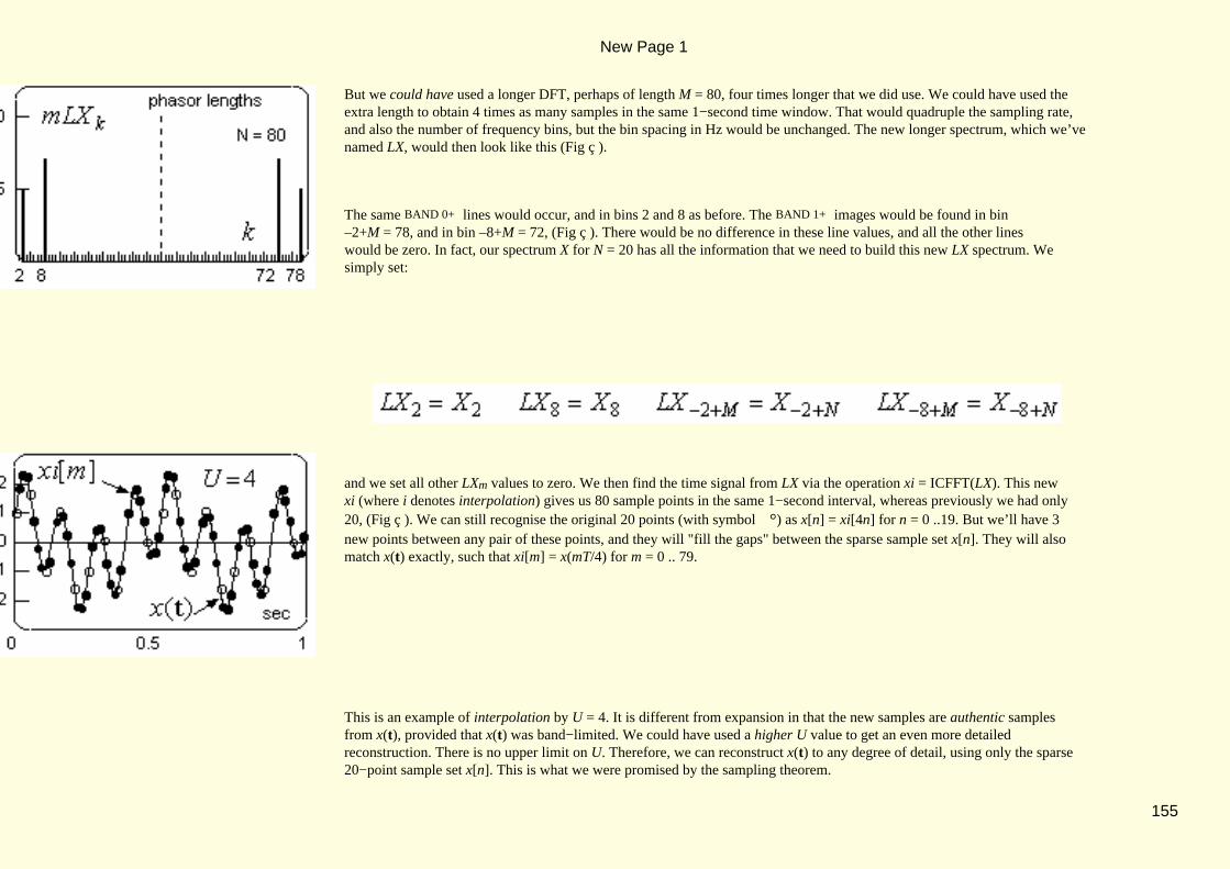
But we could have used a longer DFT, perhaps of length M = 80, four times longer that we did use. We could have used theextra length to obtain 4 times as many samples in the same 1−second time window. That would quadruple the sampling rate,and also the number of frequency bins, but the bin spacing in Hz would be unchanged. The new longer spectrum, which we’venamed LX, would then look like this (Fig ç ).

The same BAND 0+ lines would occur, and in bins 2 and 8 as before. The BAND 1+ images would be found in bin–2+M = 78, and in bin –8+M = 72, (Fig ç ). There would be no difference in these line values, and all the other lineswould be zero. In fact, our spectrum X for N = 20 has all the information that we need to build this new LX spectrum. Wesimply set:

and we set all other LXm values to zero. We then find the time signal from LX via the operation xi = ICFFT(LX). This newxi (where i denotes interpolation) gives us 80 sample points in the same 1−second interval, whereas previously we had only20, (Fig ç ). We can still recognise the original 20 points (with symbol °) as x[n] = xi[4n] for n = 0 ..19. But we’ll have 3new points between any pair of these points, and they will "fill the gaps" between the sparse sample set x[n]. They will alsomatch x(t) exactly, such that xi[m] = x(mT/4) for m = 0 .. 79.

This is an example of interpolation by U = 4. It is different from expansion in that the new samples are authentic samplesfrom x(t), provided that x(t) was band−limited. We could have used a higher U value to get an even more detailedreconstruction. There is no upper limit on U. Therefore, we can reconstruct x(t) to any degree of detail, using only the sparse20−point sample set x[n]. This is what we were promised by the sampling theorem.

New Page 1

155

We obtained LX from X by a process of spectral zero−padding. We used the lines that we had available, and then filled outthe middle of the spectrum with zeros. This did not alter the amplitude or the shape of the time signal, but it gave us a muchmore detailed set of time samples. Later on, we'll perform zero−padding on a time signal, in order to obtain a more detailed setof spectral samples. Zero padding (in whatever domain) adds no new information, but it correctly fills the spaces betweensamples in the other domain.

6.3.5 DFT Spectra of Periodic Signals

We tabulated this triangle waveform (Fig ê ) much earlier (ï Ch 4.2.3), and the diagram also shows how we can find itsCk coefficients exactly. For example, if we choose A = 1 and W/P = 0.2, we obtain:

New Page 1

156

This method relies on a derivation that gave us a formula for the Ck values. Derivations get more difficult as the waveform

shape gets more complex, but the DFT can do the same job without a derivation. If the periodic signal is x(t)~ with period P,

we take a DFT of length N, and we choose a sample interval of T = P/N. Then we form:

This time window covers exactly one period, from t = 0 to t = P. Then we find the spectrum as X = CFFT(x), and weknow that Ck' = X k. We did this for the triangle waveform using N = 32 (a power of 2), and we tabulated the Ck fromtheory and the Ck' from the DFT as far as k = 10, with this result:

k 0 1 2 3 4 5 6 7 8 9 10

Ck 0.100 0.097 0.088 0.074 0.057 0.041 0.025 0.014 0.005 0.001 0.000

Ck' 0.102 0.098 0.089 0.075 0.059 0.042 0.028 0.016 0.008 0.003 0.002

We see that the Ck' are too high in all cases. That's because of the additive effect of the aliases from higher frequencies, whichare always real and positive, because sinc2 is real and positive. To make Ck' come far closer to the true Ck , we must reducethe overlap due to aliasing. The way to do this is to use far higher N, such as N = 256, and then set T = P/N as before. Wethen get many more time samples over the same one−period time window. The sampling frequency fS = 1/T is greatlyincreased. This fS is the spacing between spectral replicas and, by increasing fS, we've reduced the amount of overlap. If we

New Page 1

157

repeat our tabulation using N = 28 = 256, we will find Ck' very close to the true Ck values. We will have harmonics up as faras ½N = 128, not because the higher harmonics are of any interest (usually), but because large N makes the lower Ck' morenearly equal to Ck.

The big advantage of the DFT method is that it works for any shape of periodic waveform. By progressively increasing theDFT length N, and monitoring the resulting Ck' , we can make a reasoned judgement as to when aliasing becomesinsignificant. This confirms our ability to view periodic−signal spectra with the help of the DFT, so long as we take care tominimise spectral aliasing.

New Page 1

158

6.4 THE NORMALISED DtFT AND THE FFT

The DtFT (Discrete−time Fourier Transform) links a discrete−time signal to its continuous periodic spectrum. The time signalis a number sequence, and it may be the sample set from some analogue pulse waveform. As such, the sequence has manypossible analogue interpretations, a different one for every band of the spectrum. This is why the specta of data sequences areinherently periodic.

We will first introduce the DtFT in terms of normalised frequency f. Afterwards, we'll see how the the DFT gives us a fastand convenient way to evaluate it.

6.4.1 The DtFT in Normalised Form

We introduced the DtFT much earlier (ï Ch 3.3.2) in the form that we see here (Fig ê ).

New Page 1

159

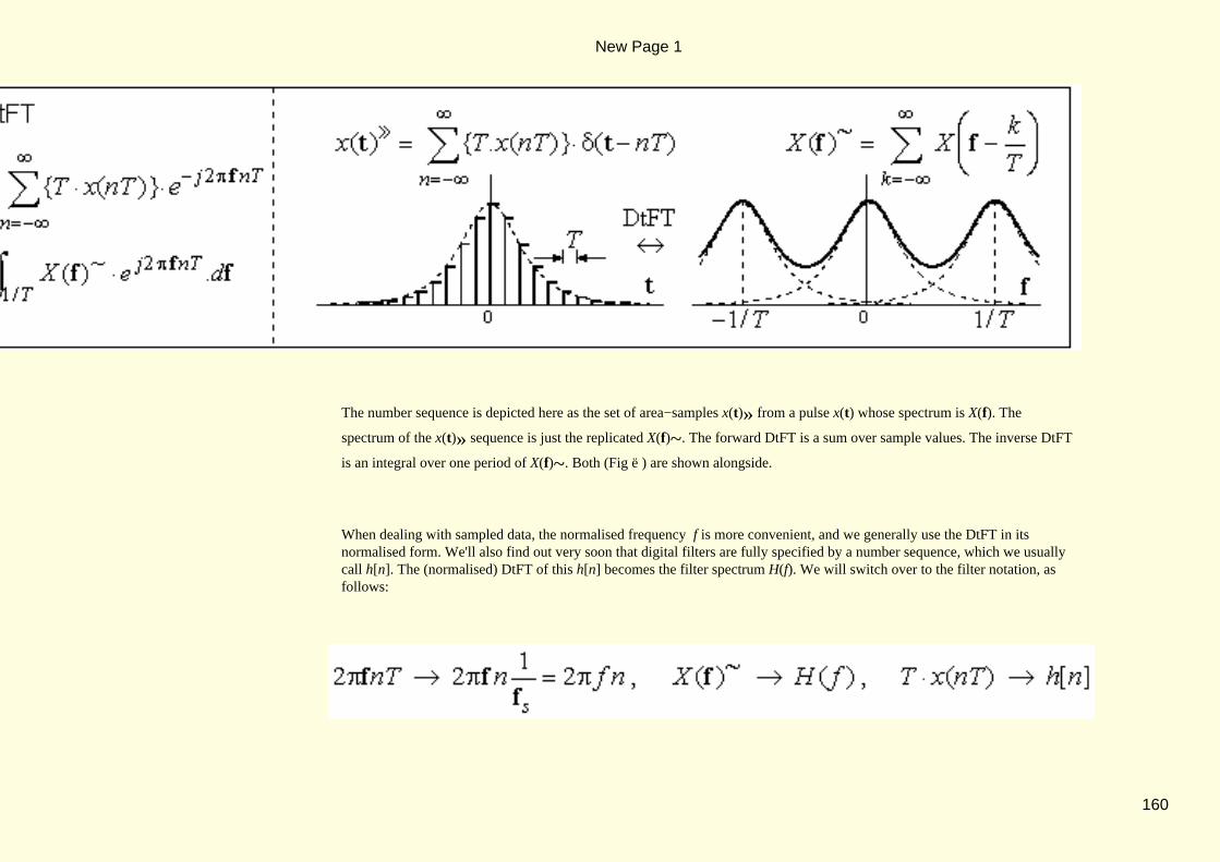
The number sequence is depicted here as the set of area−samples x(t)» from a pulse x(t) whose spectrum is X(f). The

spectrum of the x(t)» sequence is just the replicated X(f)~. The forward DtFT is a sum over sample values. The inverse DtFT

is an integral over one period of X(f)~. Both (Fig ë ) are shown alongside.

When dealing with sampled data, the normalised frequency f is more convenient, and we generally use the DtFT in itsnormalised form. We'll also find out very soon that digital filters are fully specified by a number sequence, which we usuallycall h[n]. The (normalised) DtFT of this h[n] becomes the filter spectrum H(f). We will switch over to the filter notation, asfollows:

New Page 1

160

Then the Forward DtFT summation becomes:

normalised DtFT

and the inverse integral becomes:

normalised IdtFT

This integration is over the base−band (−0.5 < f < 0.5), or over an equivalent one−period width of 1.0. The period widthis different by a factor T from the width before normalisation, which was 1/T. That is why we see h[n] = T⋅x(nT) on the left

side, instead of the x(nT) of the original form. (Also, because H(f) = X(f)~, the heights under both integral forms are

identical).

We'll make extensive use of these normalised DtFT forms. For any numeric sequence h[n] of length L, the DtFT sum gives usits periodic spectrum H(f). Computation of H(f) can be time−consuming, because it requires L complex multiplications forevery value of f in H(f). This is where the FFT can produce a time saving.

6.4.2 DtFT Evaluation by FFT

New Page 1

161

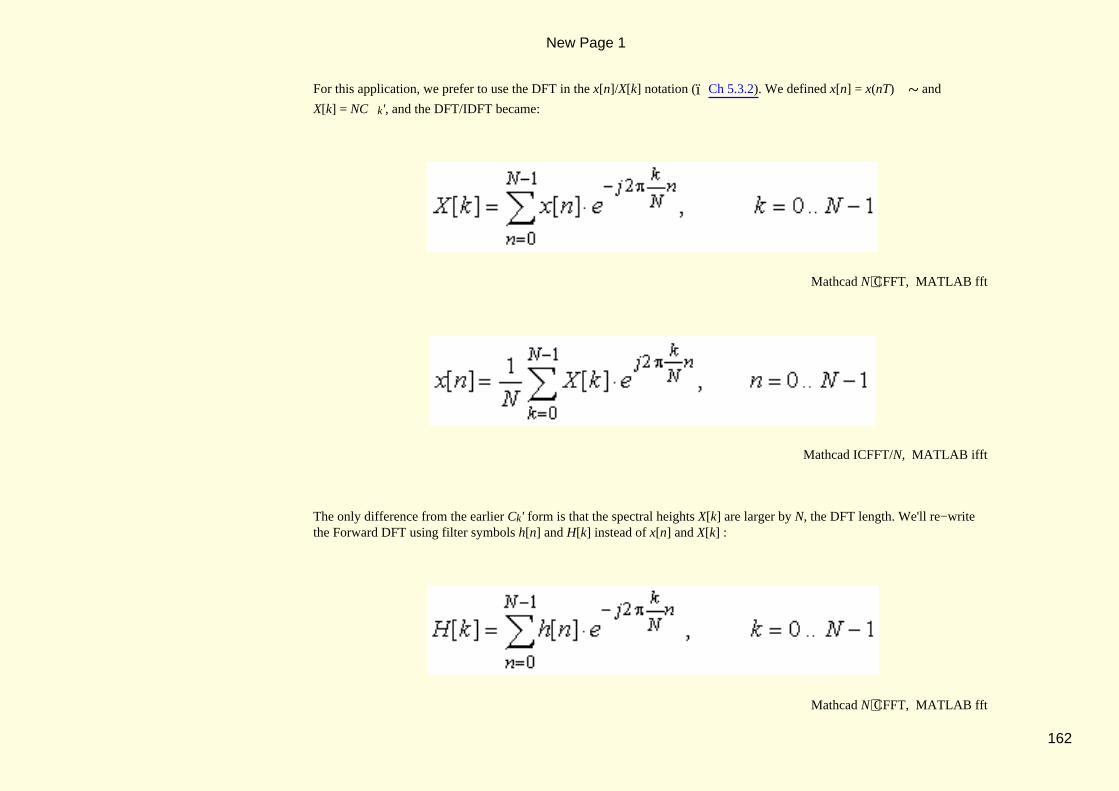
For this application, we prefer to use the DFT in the x[n]/X[k] notation (ï Ch 5.3.2). We defined x[n] = x(nT)~ and

X[k] = NC k', and the DFT/IDFT became:

Mathcad N⋅CFFT, MATLAB fft

Mathcad ICFFT/N, MATLAB ifft

The only difference from the earlier Ck' form is that the spectral heights X[k] are larger by N, the DFT length. We'll re−writethe Forward DFT using filter symbols h[n] and H[k] instead of x[n] and X[k] :

Mathcad N⋅CFFT, MATLAB fft

New Page 1

162

Now we'll write the Forward DtFT for comparison:

normalised DtFT

Direct comparison of H[k] with H(f) reveals that, provided h[n] is zero outside the range 0 .. N−1, then H[k] is a set ofN values from H(f), evaluated at the DFT bin frequencies k/N. We have to choose a DFT of sufficient length to contain all theelements of h[n]. After that, the FFT will find the filter spectrum H(f) very rapidly, at the DFT bin frequencies.

By way of an example, we'll use the following h[n] sequence:

This is a filter of length L = 5, and all of its "tap values" are 0.2. We use a DFT of length N = 128 (a power of 2), far longerthan the filter length requires. We specify h[n] for the DFT as:

This h[n] vector is of length N, as required. The filter values come first, then it is padded out with zeros to the full DFT lengthN. We compute the spectrum as

New Page 1

163

Notice the multiplication by N in this version of the DFT. We now have a spectrum with elements Hk in spectral binsk = 0 .. 127. Alongside (Fig ç ), we show the spectral magnitude plot mHk and the angle plot aHk . On the frequency axis,we've used normalised frequency k/N instead of the bin numbers k. This gives a frequency range of (0 < f < 1.0), the BAND 0+ , BAND 1+ range.

These are 128−point plots (since N = 128), but they are drawn as continuous line plots. We chose large N simply to get largespectral point density. The time−domain zero padding achieved this. It added nothing new in information terms, but it filled inthe detail of the spectrum. If we now doubled up N to N = 256, it would again halve the spectral point spacing, but the plotswould look nearly identical to what we see here.

These plots offer a full description of the filter h[n], as we will come to see in the next chapter. As such, they are veryimportant, we will use them extensively, and the FFT offers a fast and convenient framework for obtaining them.

New Page 1

164

New Page 1

165

6.5 DFT POWER AND ENERGY

When the DFT describes a periodic time signal, a DFT power spectrum is sometimes more appropriate than the normal signalspectrum. When the DFT describes a pulse in time, then the DFT energy spectrum becomes appropriate.

6.5.1 DFT Power Spectra

We demonstrated earlier (ï Ch 4.2.5) that the power associated with a phasor Ck is |Ck|2. From this, we saw that the total

signal power became:

The DFT gives us the aliased coefficients as Ck' (or as X[k]/N) and allows us to calculate mean signal power as:

New Page 1

166

total (mean) signal power

This is a summation over one DFT window, equivalent to a summation over the baseband. It gives total mean power becauseany signal power outside the baseband is aliased into the baseband when the signal is sampled. Because of this result, we canalso think in terms of bin−power, defined as:

mean power in bin−k

If we plot this, rather than plotting mXk and aXk , we obtain a DFT power spectrum, which we could also call abin−power plot. The total power is spread out over the base−band, often in a non−uniform way. We sometimes like to speakof power spectral density (PSD), which is power per unit of bandwidth. The PSD level at bin number k is the bin powerdivided by the bin−width, where bin−width is expressed in cycles per sample:

power spectral density

Notice, the normalised bin width is just 1/N. PSD and and bin−power plots give essentially the same information, but we mayfavour one over the other, depending on the application.

New Page 1

167

The power spectrum gives us only the spectral amplitudes, it contains no phase information, and hence no timing information.For signals whose timing is highly variable or unknown, we can often obtain a power specrum, even though a full X[k]spectrum might not be obtainable. This helps explain the importance of the power spectrum in many practical situations. It justtells us at what frequencies the signal power will tend to concentrate. This may be vital information. For example, if we wantto filter a transmission signal, so that it fits in a limited bandwidth, the power spectrum of the signal tells us what frequencieswe should retain, so that very little of the power will be lost.

6.5.2 DFT Energy Spectra

If the DFT time sequence x[n] describes a "one−off" pulse shape, then the signal is confined to one DFT period, which isNT in seconds, or simply N using normalised time units. Because mean power is Energy per time period, we can identify thepulse Energy as (mean power) × NT, or just as (mean power) × N using the normalised units. To convert from powerquantities to normalised Energy quantities, we just multiply by N. In this way, we get:

energy spectral density

and

energy in bin k

We can view EBINk as just ESDk × ∆f, where ∆f = 1/N.

New Page 1

168

To convert ESD and EBIN figures into time−related Energy quantities, we just multiply by T.

This concludes our first application−oriented session with the DFT. We've seen it do some jobs very well, and with the speedadvantage of the FFT to make it more attractive. But we've also hinted at some difficulties. We will tackle those difficultieswhen we next return to the DFT.

New Page 1

169

7.1 PREAMBLE

Our theoretical framework is not yet complete, and we will deal with it further in Chapter 8. Meanwhile, we want to make astart on some practical DSP work, by way of a simple introduction to digital filters. We'll begin with the sampling of somefrequently−occurring signals. Then we introduce filters of the FIR and IIR types, using the DtFT to find the filter spectra, andwe explain the importance of these spectra. We show how filters can be connected, in series and in parallel, and we introducecorrelation as a matched−filtering procedure.

New Page 1

170

7.2 SAMPLING AND SEQUENCES

The signals that we introduce here have importance in digital filtering. We will look at the sampled versions of some signalshapes x(t), and will introduce new parameters to describe these sampled versions of x(t).

7.2.1 Sampled Step and Impulse Waveforms

We will start with some elementary test signals. Prominent among these is the unit step function, defined as:

If we sample this step at sample points t = nT, the resulting sequence is u[n] :

New Page 1

171

The underline marks the zero−th element, u[0]. The double−dots denote continuation of the trend. The brackets suggestthat we treat all elements together as a single entity, as a data−sequence. The sequence is presumed to have infinite length inboth directions (−∞ < n < ∞). A different but equivalent definition is shown alongside (Fig ë ).

A slightly modified definition (Fig ç ) would show u[0] = ½. This is certainly correct for Fourier synthesis, when we try tobuild a step from sine waves. But the first definition is favoured for its simplicity, and is more widely used.

The derivative of the step u(t) is the impulse δ(t), already defined (ï Ch 3.3.2). This is easy to see if we think of the step asthe limiting case of this ramp waveform (Fig í ) when the ramp width W is reduced to zero. The derivative is a rectangle ofarea (W)(1/W) = 1.0. As W → 0, it becomes a unit−area impulse, δ(t).

We have no close digital equivalent for the impulse. The smallest meaningful W value is the sample interval T. If we samplethe rectangular−shaped derivative using W = T, we get a single sample of value 1/T, and all other sample values are zero.Thus, we can reasonably define:

New Page 1

172

digital−T impulse

as our nearest digital equivalent to an analogue inpulse δ(t). We will use this definition in the future, but it is also commonpractice to define a time−independent digital impulse as :

digital impulse

or as the "Unit Impulse" shown here (Fig ç ). This "time−free" definition is more widely−used, although it is more remotefrom the analogue impulse that gave it its name. We will use both both δ[n] and δT[n] as the situation demands.

New Page 1

173

7.2.2 Sampled Exponentials

The right−sided analogue exponential is defined by:

where a < 0 for a decaying exponential as shown (Fig ç ). Taking value−samples of x(t) with sample interval T, we get:

Even more simply:

This sequence is shown here (Fig ç ) for a = −0.14 with sample interval T = 1. The rate of decay from sample to sampledepends both on a and on T, such that the two combine to form a single decay constant, r = 0.87. This r becomes the ratio ofany sample value to the sample value just before it, that is, r = x[n]/x[n−1].

New Page 1

174

The area under the x(t) exponential (for a < 0) has a finite value, found as:

The value−samples x[n] above give no sense of this area, but the area−samples do (Fig ç ). Clearly, the sum ofarea−samples T⋅x[n] is an approximation to the area under x(t), that is:

This is true for other waveforms also. To see how it works for our exponential x(t), we must first sum the x[n] samples above.If we use SN to mean the sum over the first N samples of x[n], we have:

Now we multiply both sides by r to obtain:

New Page 1

175

Subtracting r⋅SN from SN , most terms cancel and we find:

Finally,

This is a very useful closed−form expression for SN. It continues to hold as N→ ∞, provided the sequence decays (requiringthat r < 1). Thus:

New Page 1

176

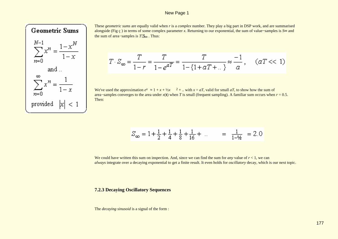
These geometric sums are equally valid when r is a complex number. They play a big part in DSP work, and are summarisedalongside (Fig ç ) in terms of some complex parameter x. Returning to our exponential, the sum of value−samples is S∞ andthe sum of area−samples is T⋅S∞ . Thus:

We've used the approximation ex ≈ 1 + x + ½x 2 + .. with x = aT, valid for small aT, to show how the sum ofarea−samples converges to the area under x(t) when T is small (frequent sampling). A familiar sum occurs when r = 0.5.Then:

We could have written this sum on inspection. And, since we can find the sum for any value of r < 1, we canalways integrate over a decaying exponential to get a finite result. It even holds for oscillatory decay, which is our next topic.

7.2.3 Decaying Oscillatory Sequences

The decaying sinusoid is a signal of the form :

New Page 1

177

where ω0 = 2πf 0 is just the radian frequency (rads/sec). After sampling:

We now have two constant parameters:

such that:

The sequence is shown here (Fig ç ) for r = 0.87 and θ = 0.5. Recall that a sine wave is a sum of two rotating phasors,and the angle θ is the amount by which the phasors rotate from one sample to the next, in units of radians/sample, adesciption which is independent of the sampling frequency. The decaying sinusoid can always be represented by a singlecomplex number r∠θ as shown here (Fig í ). The radius r gives the decay between samples, while θ is the rotation betweensamples. As long as r∠θ lies inside the circle of radius 1.0, the signal will decay, and its area under integration will be finite,because it lies within the envelope of a decaying exponential. Signals of this type, and diagrams like this, will recur again and

New Page 1

178

again in our later work.

New Page 1

179

7.3 DIGITAL FILTERS AND CONVOLUTION

Digital filters are used to modify a signal by removing (or re−shaping) some of its frequency components. The input signal isrepresented by its samples x[n], and the "filter" is just a set of calculations that are repeated over and over on the input samplesx[n], to generate a set of output samples, y[n]. The filter action repeats under control of a "clock" signal, wheren = 0,1,2 .. etc counts the clock cycles such that, on each clock cycle, the filter takes in a new input sample x[n], andoutputs a new output sample y[n]. Most often, the action of the filter can be specified by another set of samples called h[n],which is known as the "Impulse Response" of the filter (Fig ç ).

7.3.1 LTI Filters

LTI is short for "Linear and Time−Invariant". Most of our filters will be LTI filters, and their impulse response h[n] definesthem completely. It is so named because, if the input signal to the filter is the impulse sequence δ[n], (a solitary "1" at n = 0and nothing thereafter), the resulting output sequence y[n] is the sequence of numbers that we call h[n], the "response to animpulse". The filter's response to some different input sequence is determined by h[n] and by the LTI nature of the filter, andwe will illustrate this with an example.

New Page 1

180

We'll choose a filter whose impulse response is h[n] = rn.u[n] with r = 0.5. Thus:

This sequence continues indefinitely. For the input x[n], our choice is simple but arbitrary:

The filter responds to each element of x[n] in succession. At n = 0, it responds to the "1" by outputting 1 ½ ¼ etc . Theresponse to the "2" is doubled in size, and delayed by one cycle: 0 2 1 ½ etc . The response to the "3" is tripled in size anddelayed by two cycles. Similaly for the "4", and then the input terminates.

This table (Fig ê ) shows each response as a separate row. At the bottom, it adds up the responses by summing columnsvertically. The output y[n] on the last row is the sum of all the responses.

New Page 1

181

This filter showed linearity by giving a response directly proportional to the size of the input sample. It showed timeinvariance by responding to successive samples (each arriving at a different time) with a scaled version of h[n], all in the sameunvarying manner. These are the features that make it an LTI filter.

To see how y[n] is assembled, we look at the y[3] column (inside the grey box) and, on close examination, we find that:

We can generalise this result for any output sample y[n] :

New Page 1

182

Notice how n is a constant while we do a summation over m to obtain y[n]. Then we increment n by one and do the nextsummation, resulting in y[n+1]. This equation sums up the filter action, and describes a process that we call convolution. Ourtabular approach has shown this to be the natural result of linearity and time invariance. But, to better understand convolution,and to do convolution on paper, we recommend a different method, as follows.

7.3.2 Convolution of Sequences

This diagram shows the graphical method that we prefer (Fig ê ):

The first row shows h[n] in time−reversed form. The second row shows x[n] in its normal form. We've underlined the n = 0index positions and lined them up vertically, so that the first elements of each are overlapping. These are 1.000 and 1.0 on thediagram. The product of this vertical pair is y[0] = 1.000, the first output sample from the filter. Now we slide the h[n]sequence to the right, one step at a time. After one step, we have two pairs overlapping, and the output y[1] becomes the sum

New Page 1

183

of vertical product pairs y[1] = 1.0×2.0 + 0.5 ×1.0 = 2.500. After another step, we obtain y[2] as y[2] = 1.0×3.0 +

0.5×2.0 + 0.25×1.0 = 4.250. It’s easy to check that this is equivalent to the tabular method, but it gives us a better insightinto what convolution is about.

We prefer to think of sequences as covering all possible index values (−∞ < n > ∞). If we assume that x[n] and h[n] areboth zero for all n < 0, we'll see from the diagram that we can extend the limits to infinity without affecting the result.Therefore:

digital convolution

We use the special symbol * to indicate convolution:

It also turns out that:

New Page 1

184

This means that we can time−reverse x[n] rather than h[n], then continue the process as normal, and the result y[n] will be thesame as before. Therefore:

digital convolution (or filtering)

This is the commutative property of convolution.

A sequence is said to be causal if it is zero−valued for all n < 0. We convolved two causal sequences x[n] and h[n], and wefound that the output y[n] was causal too. This is true of filters in general. The output y[n] is causal because we cannot get anoutput before we apply an input. It is simply the principle of cause and effect (hence the term causal). Filtering is most oftenperformed in real time, meaning that the filter must wait for the next input sample before it can deliver the next output sample.It's not always like that. If the input data has been recorded in advance, we may have access to any input sample on demand. Ifwe avail of that, we then have a non−causal filtering action.

7.3.3 Filter Frequency Response

If a digital filter is driven by a sampled sinusoidal sequence of frequency f (in cycles/sample), the output y[n] develops into asinusoidal sequence of the same frequency, but with different amplitude and phase, as we will now demonstrate. Because asine wave is built from two phasors, we can use a sampled phasor as our input x[n], and extend our result later to sine waves.

New Page 1

185

So, we have:

Then:

Finally−− for this specific inout sequence:

= x[n] × (DtFT of h[n])

We recognise the bracketed quantity as the DtFT of h[n], which is also the filter spectum, a complex function of frequencycalled H(f). Suppose that, at some specified f value, H(f) = G∠θ. (magnitude G at angle θ radians). For a phasor input at+ f we obtain:

New Page 1

186

For a phasor input at − f (provided h[n] are real−valued) we obtain:

For a cosine input cos(2πfn), we take one−half of the sum of these inputs, and similarly for the outputs, which gives us:

Thus, if the filter spectrum is H(f) = G∠θ, the response y[n] to a cosine input will be scaled in magnitude by G, and its anglewill be altered by θ. Clearly, G and θ are functions of frequency, they are |H(f)| and argH(f). The plot of |H(f)| versus f isthe filter magnitude spectrum (mH), and the plot of argH(f) versus f is the filter angle spectrum (aH). We'll be using theseresults very shortly.

New Page 1

187

7.4 FIR FILTERS AND FILTER STRUCTURES

All of our filters do a convolution as we described, but they come in two major categories: FIR filters have a Finite−lengthImpulse Response, and we will deal with these now. IIR filters have an Infinite−length Impulse Response, and we will dealwith those in the next chapter.

7.4.1 The FIR Averaging Filter

We'll describe a 5−point averaging filter that operates in real time. At any given time, it remembers the most recent incomingsample x[n], and the four previous samples, x[n−1] back to x[n−4]. The filtering action is the repeated calculation of the outputy[n], for n = 0,1,2,3, .. etc, according to:

n = 0,1,2,3, ..

This is a familiar averaging procedure. It tends to suppress rapid changes in the output. As such, it reduces the high−frequency

New Page 1

188

parts, but has little effect at low frequency. In this diagram (Fig ç ), the filtering is drawn to resemble the graphicalconvolution method. The filter is a set of "taps" or multiplier values (depicted as small triangles), all of them 0.2 in this case,and they slides from left to right, while monitoring the most recent five samples of the signal. Each sample is multiplied by thecorresponding tap weight (0.2), and all five products are then added to form y[n]. After another step to the right, the processrepeats, and it determines y[n+1].

We took a noisy signal as our input, and performed 5−point averaging on it over 60 samples, with this result (Fig ç ). Theoutput has lost most of the rapid input variations, as expected. But there is something else as well, namely, the appearance of asignal delay. In fact, the delay effect is quite real, and is exactly two sample intervals. The reasoning is that our computedaverage y[n] is most representative of the middle of the filter window, which is at x[n−2], whereas y[n] appears two sampleslater. This reasoning applies to many FIR filters of length L (meaning L filter taps), and the delay is calculated as:

filter delay in samples = (L − 1)/2

The more usual kind of block diagram for this FIR filter looks like this (Fig ç ). It shows a chain of four delay blocks withthe label "T" to indicate a T−second delay. Each block is just a data register which holds a data value for one filter cycle, andthen passes it down the chain to the next register. The input data x[n] enters at the top of the chain, and the older data x[n−1],x[n−2], etc resides at tapping points along the chain, as shown on the block diagram. These data values are multiplied by thefilter coefficients, the triangles labelled 0.2, and added together to form the output y[n]. This output is a weighted sum of pastand present input values. From the block diagram, one can immediately write the difference equation that describes the filter

New Page 1

189

as:

This is quite a simple description, and we can understand intuitively that higher frequencies are somewhat suppressed, but weneed a more satisfactory statement of behaviour over frequency. Actually, we obtained it in the last chapter, and this (Fig ç )is the |H(f)| that we found, the filter's gain magnitude plot (ï Ch 6.4.2). It describes a gain that is close to 1.0 at lowfrequencies (below f = 0.1). Higher frequencies (up to f = 0.5, the top of the baseband) are more heavily attenuated.

New Page 1

190

The gain is zero at f = 0.2. That's because f = 0.2 indicates 1/0.2 = 5 samples per sine−wave period at this frequency.The 5−point filter "sees" exactly one sine−wave period, and the average over one period is zero. The filter averages the 5samples, their average value is zero, and so the y[n] values are zero every time. The same happens at f = 0.4 where theaverage is taken over 2 sine−wave periods, and the average is zero once again.

This 5−tap filter has a delay of (5 − 1)/2 = 2 samples. In terms of phase delay over frequency, this is a linear phase lag,expressed as:

lag angle = −2π f n (radians), with n = 2

The lag angle is greatest at f = 0.5, where it reaches −2π radians, which is one sine−wave period. This is indeed a 2−sampledelay, because when f = 0.5 we have only 2 samples per sine−wave period. Our FFT spectrum gave an angle plot argH(f)that seemed only "piece−wise linear" (Fig ë ), but that is very misleading. It has several discontinuities, all with a step size ofπ radians. These steps actually describe a change of sign on the magnitude plot. We can re−draw both plots, making themagnitude plot into a bi−polar plot (Fig ç ), and removing the steps from the angle plot (Fig í ). We now see the linearphase lag (the heavy line), and it reaches −2π when f= 0.5, as expected.

We can use these plots to find the gain and the phase at any frequency. For example, when f = 0.1, we find:

New Page 1

191

when f = 0.1

Suppose we now apply an input sinusoid at f = 0.1 :

H(f) predicts that the output sequence y[n] will be:

smaller in amplitude by 0.647, and lagging by 1.257 radians. To demonstrate that this is what actually happens, we only haveto run the difference equation over and over for n = 0,1,2,3, .. etc.

The result will be the same as we predicted. And we can do likewise for any other input frequency. That illustrates theimportance of the H(f) spectrum.

New Page 1

192

7.4.2 FIR Filter Structures

The averaging filter is just a particular case of the generalised FIR filter presented here (Fig ë ). It can be of any length L,with L coefficients or "tap values", and with L −1 delay blocks. The coefficients are named as b0, b1, b2, etc up to bL−1. Weoperate the filter by repeated execution of its difference equation:

FIR filter lengths range from L = 2 to L = several thousand. With suitable choice of coefficients, we can approximate anyof the "brick−wall" filters depicted here (Fig í ), but sharp transitions require longer filters.

If the input to this filter were δ[n], a solitary "1", it would ripple down the delay chain step by step. After the last delay, itwould exit and be forgotten. Before exiting, it passes each filter tap in turn, gets scaled by the coefficient value, and thendelivered to the output. It follows that the response to δ[n] will be:

New Page 1

193

In other words, the impulse response of an FIR filter is just the set of its coefficient values. The coefficients also decide thefilter spectrum, but we normally handle this the other way round. We specify the spectrum that we want, and we then try tofind the coefficients that will give it to us. This is the problem of filter synthesis, and we will leave this problem to a laterchapter.

New Page 1

194

7.5 IIR FILTERS AND FILTER STRUCTURES

FIR filter are popular, but they are not the most efficient computationally. IIR filters can often do a similar job with far fewercoefficients. We will use this section to introduce them.

7.5.1 The IIR Integrator

This block diagram and difference equation (Fig ç ) describe a very different kind of filer. The key difference is theappearance of y[ ] on the right−hand side. The output is no longer just a weighted sum of inputs. In this filter, earlier outputsamples are being fed back around a loop to the input. The use of feedback, and the presence of a feedback loop, are thedistinguishing marks of an IIR filter.

The feedback includes a (multiplier) coefficient r. If we set r = 1, the difference equation reads:

New Page 1

195

All new values of x[ ] are added to y[ ], so that y[n] becomes the sum of past and present x[] values. This filter is justan adding machine, but we call it an integrator. If we apply an impulse δ[n] at the input, the output becomes:

a unit step sequence

The output y[n] goes from 0 to 1 when the impulse arrives at n = 0, and remembers this value thereafter. (It does this byre−circulating the "1" in the loop on every subsequent filter cycle). This assumes that y[−1] was zero, it assumes zero initialconditions. We don't need such assumptions with an FIR filter.

Now suppose that r < 1. On every trip around the loop, the y[n] value is multiplied by r. The new response to an impulseδ[n] becomes:

If we use r = 0.87, the impulse response looks like this (Fig ç ), a decaying exponential sequence and, yes, we've seen thissequence before (ï Ch 7.2.2). This is the response of a "lossy" integrator. It loses a fraction (1−r) of its data on every cycle ofthe loop. The response decays away to zero, but never quite reaches zero. This h[n] is of infinite length, making this an IIRfilter. It is the re−circulation in the feedback loop that make IIR filter responses infinitely long.

New Page 1

196

If the input to the filter is x[n] = u[n], a unit step sequence, the response will be:

We can understand this quite readily as the result of a graphical convolution involving u[n] and h[n]. It looks like this(Fig ç ), and it tends to a limit of 1/(1 − r) as n → ∞. This is fine as long as r < 1. But, if r > 1, the response to animpulse will grow without limit. That would be described as unstable, and it cannot be allowed to happen. We must guardagains instability with IIR filters, whereas it cannot happen with FIR filters.

The DtFT gives us the spectrum:

New Page 1

197

normalised DtFT

With the help of this geometric sum (Fig ç ), it becomes:

We've plotted the magnitude mH of this H(f) over the base−band, with this result (Fig ç ). It is clearly a low−pass effect, witha peak gain of 1/(1−r) at f = 0. We could scale x[n] by (1−r) to give it a DC gain of 1.0 by writing:

With this small modification, we have an IIR averaging filter. It gives a weighted combination of the new data x[n] and theexisting sum y[n−1]. When r is small, the new data is emphasised, and older data is more quickly forgotten.

This example illustrates the major role of geometric sums in the feedback loop of an IIR filter. The impulse response is ageometric series, but the closed−form description of the series sum uses just the feedback coefficient r to describe both thestep response in the time domain, and the H(f) of the filter as well.

New Page 1

198

7.5.2 IIR Filter Structures

We've just seen a feedback section with only one feedback coefficient. More generally, we can have several feedbackcoefficients, like this (Fig ç ). We've named them with a minus as −a1, −a2, etc, because that will give the algebra a cleanerappearance later. This is quite a complex filter, with a difference equation:

More generally however, we allow an IIR filter to have an FIR section as well. Here (Fig ê ) we see an FIR section followedby an IIR section. This is sometimes called the Generalised Form 1, and we can write its difference equation on inspection as:

New Page 1

199

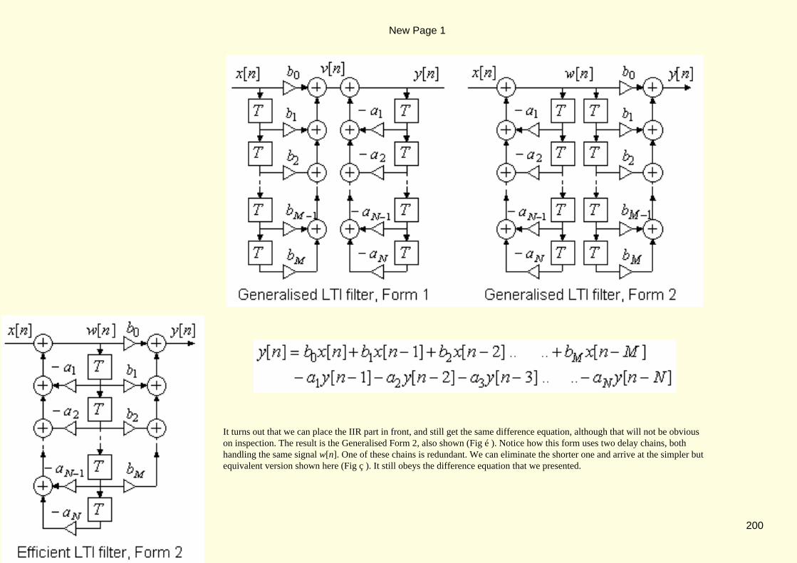
It turns out that we can place the IIR part in front, and still get the same difference equation, although that will not be obviouson inspection. The result is the Generalised Form 2, also shown (Fig é ). Notice how this form uses two delay chains, bothhandling the same signal w[n]. One of these chains is redundant. We can eliminate the shorter one and arrive at the simpler butequivalent version shown here (Fig ç ). It still obeys the difference equation that we presented.

New Page 1

200

When IIR filters use fixed−point arithmetic, the numeric truncation can give rise to complex and unwelcome non−idealeffects. That is much of the reason why long filters of this kind are seldom used. The IIR filter that has only two delays is a"second−order" filter, often called a "bi−quad" (or bi−quadratic section). It is a widely used building block (Fig ç ) with thedifference equation:

bi−quad

We will use this block quite frequently. It is all that we need to build IIR filters because we can combine several bi−quads inseries or in parallel to build filters of higher order. That will be our next topic.

7.5.3 Filter in Series and in Parallel

Almost all of our filters are LTI filters (linear and time−invariant), and this allows us to easily combine them in series or inparallel. Very often, the individual filters will be bi−quads, but other LTI filters can be used as well.

The parallel connection is very simple (Fig ç ). We're just adding the outputs of (two or more) individual filters. That's thesame as adding their individual impulse responses. It also means that we can add the two filter spectra to get an equivalentfilter spectrum H(f).

New Page 1

201

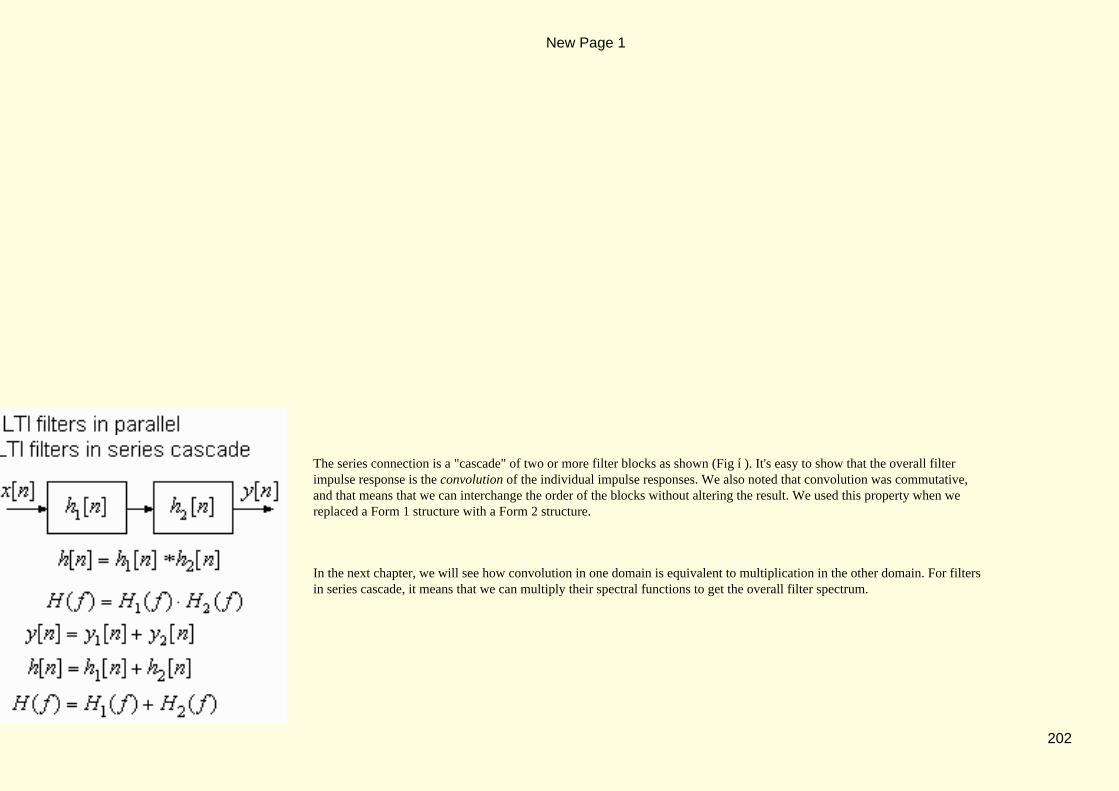
The series connection is a "cascade" of two or more filter blocks as shown (Fig í ). It's easy to show that the overall filterimpulse response is the convolution of the individual impulse responses. We also noted that convolution was commutative,and that means that we can interchange the order of the blocks without altering the result. We used this property when wereplaced a Form 1 structure with a Form 2 structure.

In the next chapter, we will see how convolution in one domain is equivalent to multiplication in the other domain. For filtersin series cascade, it means that we can multiply their spectral functions to get the overall filter spectrum.

New Page 1

202

Later on, we will learn how to design bi−quads for series or parallel connection, so as to implement filters that can meet somespecified H(f) description.

New Page 1

203

7.6 CORRELATION METHODS

Some filters have a purpose somewhat different from the norm. Their job is to recognise a certain known pattern of inputsamples x[n]. Recognition would be easy except that the known pattern x[n] may be heavily corrupted by noise (as when wetry to recognise radar pulses after they have been reflected from an aircraft). That calls for a filter which responds morestrongly to the expected x[n] pattern that to any other input sequence. It is known as a matched filter.

7.6.1 The Matched Filter Concept

The output from a filter is a sum of products. The idea of a matched filter is to incorporate the x[n] "signature" in the detectionfilter in a way that will maximize the sum of products for the anticipated x[n]. A maximized sum, with x[n] as one of thesequences, would be the sum of the squared x[n] values (times an arbitrary scale factor). We can get this result from an FIRfilter whose impulse response h[n] is a time−reversed version of the expected input sequence x[n]. This example uses anarbitrary x[n] of length six (Fig ê ). To match this x[n], we need a filter described by h[n] = 5 −4 3 −1 2 1 , acausal time−reversed copy of x[n]. To perform the convolution, we must flip h[n] as shown, then slide it across the x[n]sequence:

New Page 1

204

The output y[n] will be maximised when n = 5, with a value of:

the total energy in x[n]

The peak output is also the energy of the x[n] sequence. If there is added noise, the noise terms will tend to cancel rather thanto accumulate. Whenever y[n] reaches a peak that exceeds some agreed threshold, we conclude that the expected x[n] has beendetected.

7.6.2 Cross−correlation and Auto−correlation

In the above illustration, we took two identical number sequences and we slided one across the other until we found a match(at n = 5), as indicated by the peaking of the output sequence y[n]. When the sequences are identical, this kind of action iscalled auto−correlation. But, in a practical detection filter, the input x[n] will have added noise, and will not be identical toh[n]. We are then comparing two different sequences, and we are looking for some similarity between them, as indicated by apeaking of y[n]. This is called cross−correlation, and a matched filter is a cross−correlator that (usually) works in real−time.

New Page 1

205

For sequences x1[n] and x2[n], the cross−correlation sequence is:

It looks very like a convolution. The only difference is that we used x1[m − n] rather than x1[n − m]. It means that unlikeconvolution, when we do this operation on paper, we do not reverse one of the sequences beforehand.

Here is a simple example of a cross−correlation of two causal sequences of lengths 5 and 6 respectively (Fig ê ). We writeboth sequences as given, then we slide the upper sequence to the left and to the right, computing sums of products until nooverlap remains. The result r12[n] is of length 10, one less than the sum of the sequence lengths, and the result is not causal (ithas non−zero values at negative indexes, and the maximum similarity is found at n = −1). If this were a convolution, theresult y[n] would again have length 10, but it would be a causal sequence.

Cross−correlation and convolution are similar in that the same numeric algorithm can be used to do both. (The difference is inwhether we reverse one sequence before we enter it). But they are very different in other ways. Convolution is usually areal−time operation, one that uses new data as it becomes available. With correlation, we would often have all of the data tohand before doing a comparison. Cross−correlation is the fudamental operation that underlies identification methods asperformed by a computer (as in fingerprint matching, voice recognition, etc).

New Page 1

206

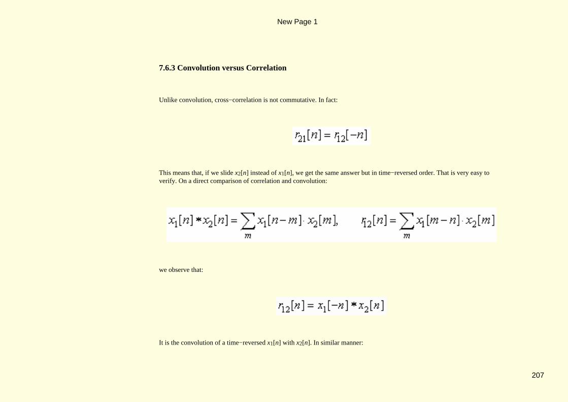
7.6.3 Convolution versus Correlation

Unlike convolution, cross−correlation is not commutative. In fact:

This means that, if we slide x2[n] instead of x1[n], we get the same answer but in time−reversed order. That is very easy toverify. On a direct comparison of correlation and convolution:

we observe that:

It is the convolution of a time−reversed x1[n] with x2[n]. In similar manner:

New Page 1

207

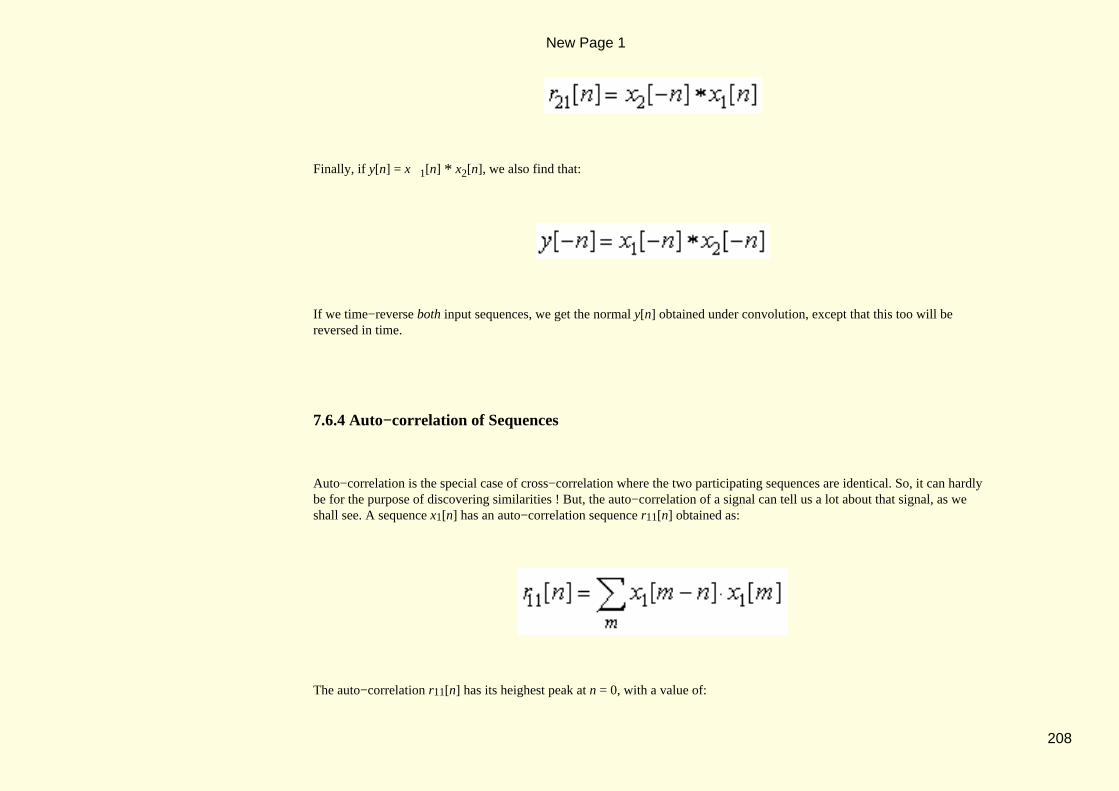
Finally, if y[n] = x 1[n] * x2[n], we also find that:

If we time−reverse both input sequences, we get the normal y[n] obtained under convolution, except that this too will bereversed in time.

7.6.4 Auto−correlation of Sequences

Auto−correlation is the special case of cross−correlation where the two participating sequences are identical. So, it can hardlybe for the purpose of discovering similarities ! But, the auto−correlation of a signal can tell us a lot about that signal, as weshall see. A sequence x1[n] has an auto−correlation sequence r11[n] obtained as:

The auto−correlation r11[n] has its heighest peak at n = 0, with a value of:

New Page 1

208

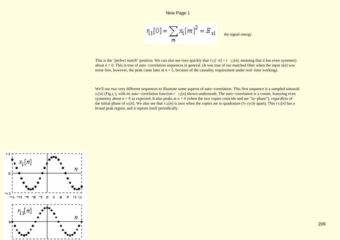
the signal energy

This is the "perfect match" position. We can also see very quickly that r11[−n] = r 11[n], meaning that it has even symmetryabout n = 0. This is true of auto−correlation sequences in general. (It was true of our matched filter when the input x[n] wasnoise free, however, the peak came later at n = 5, because of the causality requirement under real−time working).

We'll use two very different sequences to illustrate some aspects of auto−correlation. This first sequence is a sampled sinusoidx1[n] (Fig ç ), with its auto−correlation function r11[n] shown underneath. The auto−correlation is a cosine, featuring evensymmetry about n = 0 as expected. It also peaks at n = 0 (when the two copies coincide and are "in−phase"), regardless ofthe initial phase of x1[n]. We also see that r11[n] is zero when the copies are in quadrature (¼ cycle apart). This r11[n] has abroad peak region, and it repeats itself periodically.

New Page 1

209

The second example is a random noise sequence (Fig í ), with its auto−correlation sequence r[n] shown underneath. We'venot shown the n < 0 part, because the symmetry makes it unnecessary. It has one very large value ( > 60) when n = 0, andquite small values everywhere else. This is easily explained. When n = 0, we are comparing two identical copies, and theresult is the total energy (or sum of squares). But, with random noise, any sample is unrelated to the sample beside it, so thateven for n = 1, we are comparing two entirely different sequences, and the sum of products will tend toward zero as anaverage (provided the sequence has no DC component). This r[n] has a very narrow peak region (one sample wide), in fact, ittends toward K⋅δ[n] in the limit as more and more input samples are included.

Based on these examples, we can appreciate the following. Noise sequences have little predictability from sample to sample,they have a wide range of frequencies, and they have a narrow auto−correlation peak. If the noise signal is then low−passfiltered, the higher frequencies are removed, it becomes more slowly varying, there is much greater predictability from sampleto sample, and its auto−correlation peak becomes very much wider.

The auto−correlation r[n] sequence says much about the frequency content of a signal. Later on, we will see how its Fouriertransform is also the signal's power spectrum. As such, it tells us all about signal amplitudes over frequency, but it tells usnothing about the phase (or the timing information).

To sum up, convolution is about filtering a signal, cross−correlation is about comparing two signals, and auto−correlation isabout the properties of a signal. This has been just a brief introduction, with much more to be said later on.

New Page 1

210

New Page 1

211

8.1 PREAMBLE

One way to design a digital filter is to have it mimic the action of a known analogue filter such that, as the sample intervalT → 0, they become more nearly alike. By letting T → 0 with our digital filter, we will arrive at an analogue filter model, andat an integral that describes analogue convolution. We will also see the analogue equivalents of cross−correlation andauto−correlation.

To assist us in this effort, we will also need the spectral view that the Fourier Transform (FT) can provide. Although we'veencountered the FT in several guises, we have yet to document the FT properties and the FT pairs that will be useful to us.We'll present these initially in terms of the CFT, but we'll extend them where appropriate to cover other useful forms.

New Page 1

212

8.2 ANALOGUE FILTER DESCRIPTIONS

This section will take us from operations on sequences to the corresponding operations on analogue signals, and will give usthe time−domain models that we use for linear analogue processing of signals.

8.2.1 From Digital to Analogue

This diagram (Fig ê ) shows the digital filter as approximating the action of an analogue filter.

New Page 1

213

The filter generates the output sequence as y[n] = x[n] * h[n]. In order that the time scale is included, we treat these numbersas area−samples (rather than value−samples) of corresponding analogue signals, namely, y(t), x(t) and h(t). We can thereforewrite the convolution as:

or as:

We're free to divide across by T. That gives us the option to think of x[n] and y[n] as value−samples, if we prefer, but wemust continue to think of h[n] as area−samples of an analogue impulse response h(t). We will go with this option, becausevalue−samples are the norm for practical purposes, so we now have:

and

New Page 1

214

If we now let T → 0, the summation becomes an integral with continuous time variables replacing the discrete time steps:

and resulting in:

the convolution integral

We've seen how, with digital convolution, we could interchange the roles of x[n] and h[n]. The same is true here:

the convolution integral

In both these forms, t is the real−time variable, and τ is a dummy time variable for the integration. For an integration inprogress, t is just a constant that sets the position of h(−τ), or of x(−τ), these being the time−reversed versions of h or

New Page 1

215

x respectively.

8.2.2 Analogue Convolution and Correlation

As an illustration of analogue convolution by the graphical method, we will convolve the x(t) of plot (a) with the h(t) of plot(b) as shown here (Fig ê ).

These regular shapes make it easy to do. In plot (c), we time−reverse x(τ) and we slide it past h(τ), computing the the areaunder the product as we go. This area will be the convolution result, y(t) = x(t) * h(t). We've shown it at t = 6, where the

area under the product is made up of three parts, namely, (3×2×2) =12, plus (2×2×2) =8, plus (1×3×2) =6, for a total areaof 26. This is the value of y(6). After several other similar calculations, we get the result shown here (Fig ç ). Carefulchecking of this example should result in a good understanding of analogue convolution.

New Page 1

216

Analogue correlation is like analogue convolution except that we do not reverse one of the signals before we integrate. UsingRxy(τ) to mean the cross−correlation of x(t) with y(t), the correlation integral is:

As usual, t is the real−time variable. The time variable τ represents the relative displacement of x(t) from y(t) at which we aretesting for similarity. For an integration in progress, τ is a constant, and is the lateral shift of x(t) for this comparison. But x(t)is not reversed in time. To illustrate, we will use the same two signals as we did for the convolution example, but we willre−name h(t) as y(t) to avoid any impression of filter action. These are just two arbitrary signals x and y that we wish tocompare (Fig ê ).

In plot (c), x(t) has been moved to the right by 4, but not reversed. The sum of areas becomes (2×1×2) =4, plus (1×3×2) =6,a total of 10, which is Rxy(4). After several other similar calculations, we get the result shown here (Fig ç ). Careful checkingof this example should result in a good understanding of analogue cross−correlation.

New Page 1

217

Analogue auto−correlation is no different, except that we use the same signal twice over. This (Fig ç ) is a plot of Rxx(τ), andit has the expected peak at τ = 0, and the expected even symmetry as well. Also, the information that Rxx(τ) gives us aboutx(t) is the same as in the digital case.

8.2.3 Convolution with Impulses

The impulse response of a digital filter is a complete filter description. We can expect a similar result for analogue filters,which means that, when the input to the filter is the analogue impulse function δ(t), the filter output will be its analogueimpulse response h(t), and this too is a complete filter description.

The analogue impulse δ(t) is infinitely tall and infinitely narrow, and has unit area. The nearest approximation, for digitalworking, would be a pulse of width T and height 1/T, where T is the sampling interval. The value−samples from this pulsewould be δT[n], with a sample of value 1/T at n = 0, and all zeros elsewhere.

New Page 1

218

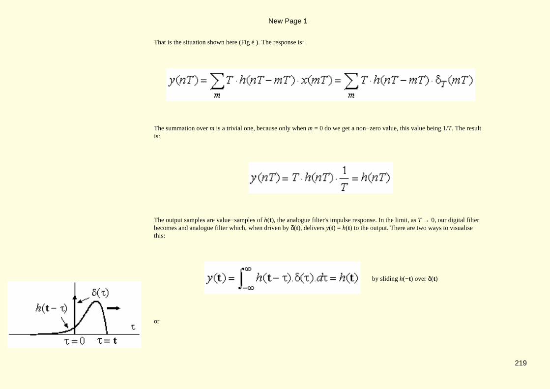
That is the situation shown here (Fig é ). The response is:

The summation over m is a trivial one, because only when m = 0 do we get a non−zero value, this value being 1/T. The resultis:

The output samples are value−samples of h(t), the analogue filter's impulse response. In the limit, as T → 0, our digital filterbecomes and analogue filter which, when driven by δ(t), delivers y(t) = h(t) to the output. There are two ways to visualisethis:

by sliding h(−t) over δ(t)

or

New Page 1

219

by sliding δ(−t) over h(t)

We can time−reverse h(τ) and slide it past δ(τ) as shown (Fig ë ), or we can time−reverse δ(τ) and slide it past h(τ), like this(Fig ç ). Notice, reversal of δ(τ) has no effect. In both cases however, the product of h and δ yields an impulse of area h(t)which, on integration, becomes the filter output, y(t) = h(t). Thus:

The sliding action is a scanning of h(t) by the impulse δ(t) which, under convolution, yields an exact copy of h(t). Becauseδ(t) is the "perfect" impulse, the result of the scan is a "perfect" copy of h(t).

We'll meet other situations where a signal is scanned by an approximate impulse shape, resulting in a less−than−perfect copyof the signal. This is illustated here (Fig î ).

New Page 1

220

The signal is a triangle, and is convolved with (or scanned by) a tall narrow rectangular pulse of unit area, located at timet = t 1. The result is a rather "blurred" triangle, right−shifted by t1 seconds. Sharp corners have been smoothed, because ofthe finite resolving power of the approximate impulse. If we could let T→ 0, the impulse would become a perfect one, andthe blurring would disappear. We can see all this intuitively from our understanding of analogue convolution. The concept isan important one, because it models many real−world measurement situations, where the result of the measurement isfrequency−limited by the finite resolving power of the measuring device, which in turn is modelled by a less−than−perfectimpulse shape. Indeed, a filter described as h(t) could be the model for our measuring instrument, and the measure of itsperformance is the closeness of h(t) to the ideal impulse shape. Ideally, we would have h(t) = δ(t), so that the measuredresponse to an impulse at the input becomes y(t) = δ(t), a perfect reproduction of that impulse.

New Page 1

221

8.3 CFT PROPERTIES

To further our work with filters, and in other areas too, we will revisit the CFT and its properties, and we will tabulate someCFT pairs. We will later extend our findings to the DtFT, which we use to obtain the spectra of digital filters.

8.3.1 CFT Properties

We will list several properties (Fig ê ) of the CFT. They are easily proved, and many of them simply mirror observations thatwe made earlier about sine waves and Fourier Series, so they should come as no surprise.

New Page 1

222

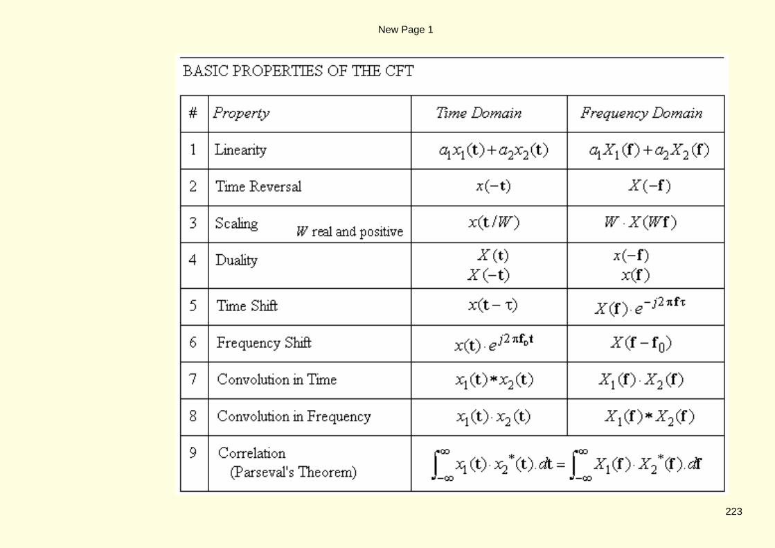
New Page 1

223

We will comment briefly on each. Property 1, linearity, is vital. It says that the response is directly proportional to thestimulus, and it allows us to superimpose the results from two or more stimuli. Without linearity, attempts at analysis aregreatly complicated. Linearity is a basic premise in nearly all that we do.

Property 2, time reversal, mirrors our earlier experiences with isolated sine waves, and with Fourier Series waveforms. It we"flip" the time pulse, then we "flip" the spectral description as well. For real−valued time signals, the flipped spectrum X(−f)is the same as X*(f), because of the even−magnitude, odd−phase spectral symmetry.

Property 3, scaling, is one that we use a lot, and should be clearly understood. The scaling parameter W is assumed to be apositive real number. Let us suppose that W is greater than 1. Then x(t/W) is a version of x(t) that has beenstretched horizontally by a factor W. Its spectrum, W · X(W f ), is a version of X(f) that has been compressed horizontally, withscale factor (1/W), but it has also been stretched vertically by a factor W. Overall, the area of W⋅X(Wf) remains unchanged bythe scaling. We can summarise the scaling action as follows:

When a pulse waveform undergoes horizontal expansion (or compression) in one domain, its counterpart in the otherdomain undergoes compression (or expansion), and also a height adjustment, such that its area does not change.

•

This is most important, because it allows us to define transform pairs from basic pulse shapes, and to adjust their dimensionslater using the scaling rule. We will use this rule extensively. But property 1 (linearity) also has a role in re−shaping a pulse: ifwe change the pulse height in one domain, then from linearity, the height in the other domain follows suit.

Property 4, duality, exploits the symmetry that we have already noted. It uses the fact that the forward CFT and the inverseCFT are identical, except for the sign in the exponent. They differ only in the direction of rotation of the phasor term. Property4 is the general result , which we have written in two alternative forms. But note also that, if a function x( · ) has evensymmetry, then x(−f) = x(f) and we can directly swap x(t) with X(f) to get a new transform pair. We will see examples of thisshortly.

New Page 1

224

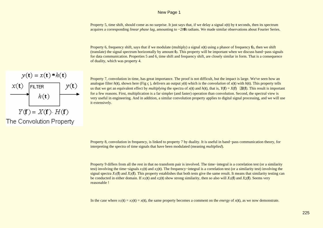
Property 5, time shift, should come as no surprise. It just says that, if we delay a signal x(t) by t seconds, then its spectrumacquires a corresponding linear phase lag, amounting to −2πft radians. We made similar observations about Fourier Series.

Property 6, frequency shift, says that if we modulate (multiply) a signal x(t) using a phasor of frequency f0, then we shift(translate) the signal spectrum horizontally by amount f0. This property will be important when we discuss band−pass signalsfor data communication. Properties 5 and 6, time shift and frequency shift, are closely similar in form. That is a consequenceof duality, which was property 4.

Property 7, convolution in time, has great importance. The proof is not difficult, but the impact is large. We've seen how ananalogue filter h(t), shown here (Fig ç ), delivers an output y(t) which is the convolution of x(t) with h(t). This property tellsus that we get an equivalent effect by multiplying the spectra of x(t) and h(t), that is, Y(f) = X(f)⋅H(f). This result is importantfor a few reasons. First, multiplication is a far simpler (and faster) operation than convolution. Second, the spectral view isvery useful in engineering. And in addition, a similar convolution property applies to digital signal processing, and we will useit extensively.

Property 8, convolution in frequency, is linked to property 7 by duality. It is useful in band−pass communication theory, forinterpreting the spectra of time signals that have been modulated (meaning multiplied).

Property 9 differs from all the rest in that no transform pair is involved. The time−integral is a correlation test (or a similaritytest) involving the time−signals x1(t) and x2(t). The frequency−integral is a correlation test (or a similarity test) involving thesignal spectra X1(f) and X2(f). This property establishes that both tests give the same result. It means that similarity testing canbe conducted in either domain. If x1(t) and x2(t) show strong similarity, then so also will X1(f) and X2(f). Seems veryreasonable !

In the case where x1(t) = x2(t) = x(t), the same property becomes a comment on the energy of x(t), as we now demonstrate.

New Page 1

225

The integrals become:

For any vector v, the product v·v* equals the squared magnitude, |v|2. We have two instances of this here, so that the integralsreduce to:

= total signal energy

The left side is what we defined as the total energy of x(t), and the right side now emerges as an alternative energy measure,expressed in terms of X( f ). Both these measures are of the same form. |x(t)|2 is energy per unit time, better known as power.|X(f)|2 is energy per unit bandwidth, in Hertz, better known as energy spectral density.

8.3.2 Basic CFT Pairs

We will now assemble a small collection of "fundamental" CFT pairs. We will meet other pairs too, but those pairs are easilyderived from the pairs shown here, with the help of the CFT properties which we listed.

New Page 1

226

The CFT pairs are tabulated below (Fig ê ). Pair 1 connects an impulse in time to a phasor in frequency. We can prove this inone line, as follows:

To explain this, if we take any continuous x(t), in this case a phasor, and multiply it by the unit−impulse δ(t − τ), the productis an impulse at time t = τ, with a strength equal to x(τ). When we then integrate over the impulse, the answer is the impulsestrength, x(τ).

New Page 1

227

New Page 1

228

Though the proof is easy, the interpretation may seem otherwise. But consider the special case which occurs if there is nodelay. By setting τ = 0 we get:

It says that an impulse has a flat frequency spectrum; it contains all frequencies in equal measure. For the more general case,we can read:

× (linear−phase lag of −2πfτ radians)

Thus the spectral amplitude is 1.0 at all frequencies and the phasor term merely accounts for the τ−second delay. We see that asimple time delay translates into a phasor function of frequency.

We gave a proof of Pair 2 much earlier (ï Ch 3.2.2). The "sinc" shape of the spectrum X(f) suggests that a rectangular pulsehas predominantly low frequencies, but it has a noticeable content at much higher frequencies as well. The latter are necessaryfor the construction of fast changing edges, which are the step−wise boundaries of the time−pulse

Pair 3 is easily deduced from pair 2 using property 7, convolution in time, and it follows from the fact that Λ(t) is theconvolution of Π(t) with itself, that is:

New Page 1

229

This convolution is easy to visualise. Then, by property 7, the spectrum of Λ(t) is sinc(f) · sinc(f) = sinc2(f). This transformpair will later find use in some practical engineering applications. This pair also accounts for the X( f ) that we used earlier todescribe a triangular pulse train, when we said (ï Ch 4.2.3):

To arrive at this result, we first take the shape Λ(t), we multiply it by A for a peak height of A, and then we stretch it by½W for a pulse width of W. The scaling rule compresses the sinc2 spectrum by ½W, and also grows its height by ½W. Thataccounts for the X( f ) given here. The factor A comes from linearity, because when we scale any x(t) by A , the spectrum X( f )is also scaled by A .

8.3.3 Derived CFT Pairs

From the Table of Basic CFT Pairs, and using the tabulated CFT properties, several new pairs are easily obtained. As a firstexample, we will apply the Duality property X(−t) ↔ x(f) to Pair 1 above, while also re−naming the constant τ as afrequency constant f1. The result is Pair 4 in the Table of Derived CFT pairs below (Fig ê ). This describes a familiarsituation. A phasor time−function of frequency f1 is represented in frequency by a single impulse at frequency f1. We used thisconcept for Fourier Series spectra, except that the impulse was then called a line. Both have the same meaning. The length ofthe line is the strength of the impulse, and they are both described in digital terms by a number.

Both of the CFT pairs numbered 2 and 3 use time functions x(t) which have even symmetry. Thus, x(−t) = x(t), and the dualityproperty then permits us to interchange the roles of x(t) and X(f) directly. The CFT pairs 5 and 6 then follow at once. Pairnumber 5 has wide application because the rectangular frequency function can be scaled to describe an ideal low−pass filter.We will see more of this later.

New Page 1

230

New Page 1

231

Pair 7 is easily derived from pair 4. We take two instances of pair 4. The first is at frequency f1 and is scaled by ½∠α :

The second is at frequency −f1 and is scaled by ½∠−α :

Now we add these two pairs on both sides. The left side becomes a sinusoid of angle α. The right side becomes a pair ofimpulses at ± f1 with strengths of ½∠(α) and ½∠(−α) respectively. It is identical to the line spectrum of a sinusoid, exceptthat line lengths are replaced by impulse strengths. Notice, the scaling and addition used in this example are both dependenton the linearity of the CFT.

Pair 8 is a special case of pair 1. We can also arrive at it from a scaled version of pair 2 as follows:

The time pulse on the left has width W, height 1/W, and unit area. As we let W→ 0, this pulse approaches impulsive shape,while the sinc on the right spreads itself horizontally to approach a constant level of 1.0 in the limit. Pair 8 is the result after

New Page 1

232

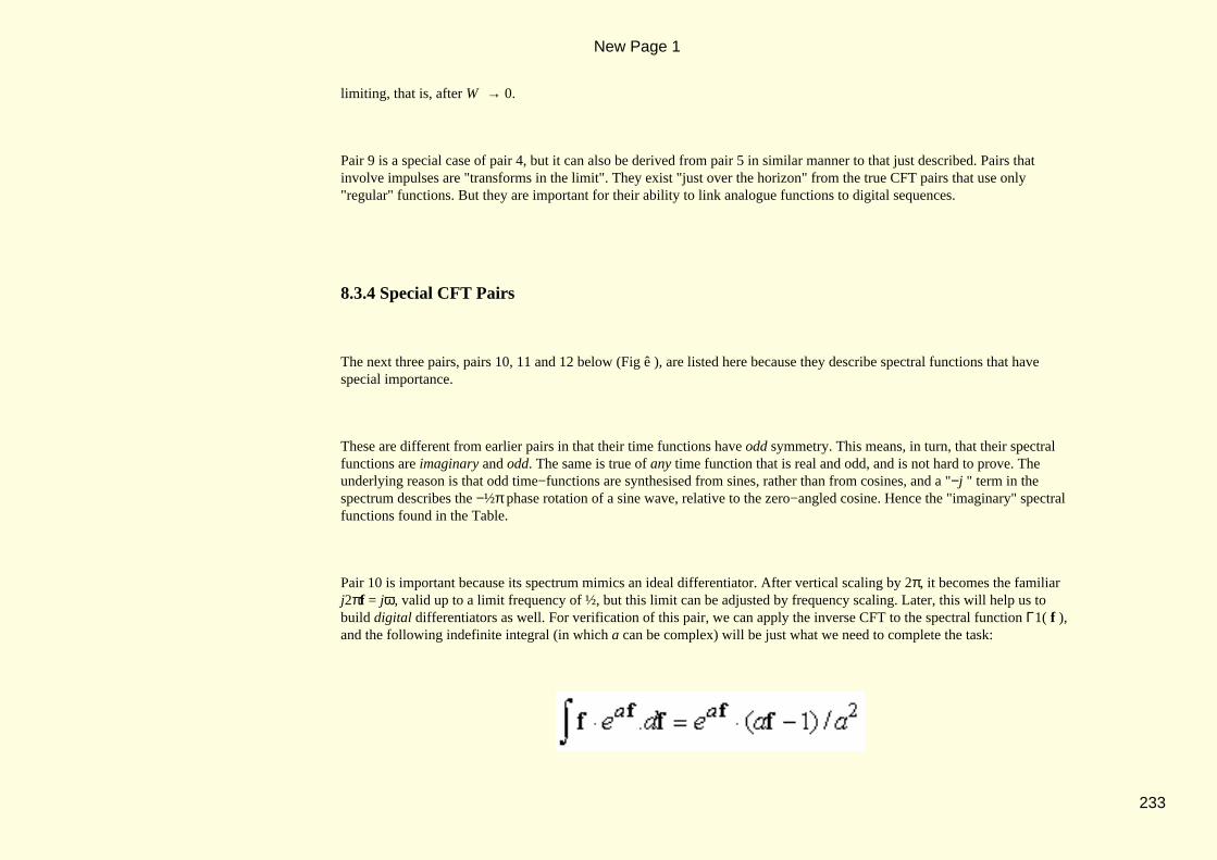
limiting, that is, after W→ 0.

Pair 9 is a special case of pair 4, but it can also be derived from pair 5 in similar manner to that just described. Pairs thatinvolve impulses are "transforms in the limit". They exist "just over the horizon" from the true CFT pairs that use only"regular" functions. But they are important for their ability to link analogue functions to digital sequences.

8.3.4 Special CFT Pairs

The next three pairs, pairs 10, 11 and 12 below (Fig ê ), are listed here because they describe spectral functions that havespecial importance.

These are different from earlier pairs in that their time functions have odd symmetry. This means, in turn, that their spectralfunctions are imaginary and odd. The same is true of any time function that is real and odd, and is not hard to prove. Theunderlying reason is that odd time−functions are synthesised from sines, rather than from cosines, and a "−j " term in thespectrum describes the −½π phase rotation of a sine wave, relative to the zero−angled cosine. Hence the "imaginary" spectralfunctions found in the Table.

Pair 10 is important because its spectrum mimics an ideal differentiator. After vertical scaling by 2π, it becomes the familiarj2πf = jω, valid up to a limit frequency of ½, but this limit can be adjusted by frequency scaling. Later, this will help us tobuild digital differentiators as well. For verification of this pair, we can apply the inverse CFT to the spectral function Γ1( f ),and the following indefinite integral (in which a can be complex) will be just what we need to complete the task:

New Page 1

233

Pair 11 is important because its spectrum mimics an ideal phase shifter. All frequency components up to a certain limit arephase−retarded by π/2 , but their amplitudes are not altered. Phase shifters are especially useful in band−pass signalprocessing, and this result will help us to build digital phase shifters too. For verification of this pair, we can apply the inverseCFT to the spectral function Γ2(f), and the solution soon emerges without difficulty.

New Page 1

234

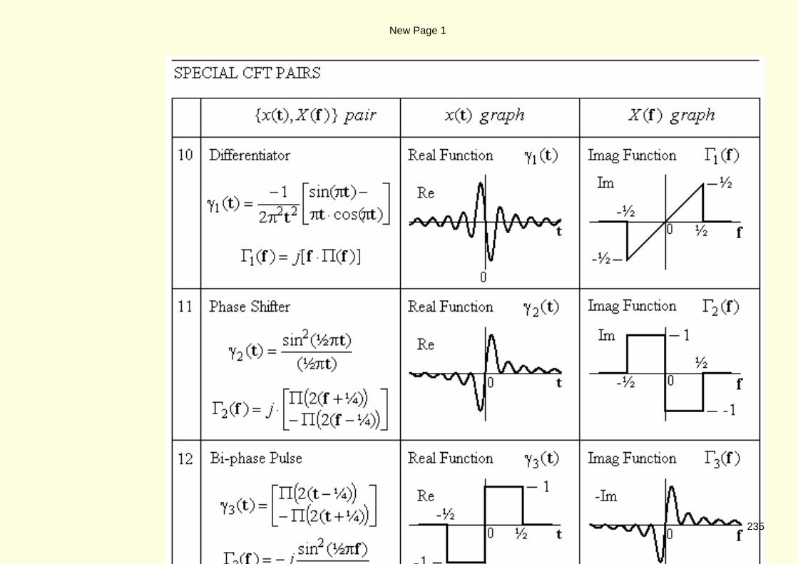
New Page 1

235

Pair 12 is the dual of pair 11, and is obtained from pair 11 using CFT property 4. The time pulse, in this case, is in the shape ofthe bi−phase pulse that is used by Manchester line code. We'll see later how the square of its spectral pulse, Γ3(f), is also thepower spectral density for Manchester−coded data streams.

8.3.5 Railings Transform Pairs

We arrived at the Railings Pairs (Fig ê ) before our current work with the CFT (ï Ch 4.3.1), but we can also regard them asCFT pairs in the limit.

New Page 1

236

They are neatly summarised by the statements:

an area−sampler transforms to a value sampler• a value−sampler transforms to an area−sampler•

As previously noted, multiplication of a signal x(t) by Railings serves to sample the signal, yielding an impulse sequence withimpulse strengths x(nT) for a value−sampler, or T⋅x(nT) for an area−sampler.

New Page 1

237

We also saw (ï Ch 8.2.3) how convolution of a signal with an impulse δ(t) amounted to a scanning action which reproducedthe signal exactly. Because Railings are a set of equally−spaced impulses, convolution of a signal with railings serves toreplicate the signal, one replica for each impulse in the train. The replicas have the same spacing as the impulses, and thisspacing becomes the period of the resulting periodic waveform. If we convolve a signal with a value−sampler, that signal isreplicated, but its amplitude is not scaled.

When we use Railings with the Convolution Properties, 7 and 8 as tabulated, they assume added significance. We now see thatmultiplication in one domain by an area−sampler is equivalent to convolution in the other domain with a value−sampler. Theresult on one side is a set of area−samples. The result on the other side is replication without scaling. The outcome is a resultthat we already know, namely, that area−sampling in one domain equates to replication in the other domain. There's nothingnew here, but the idea of Railings may help to re−inforce our pictorial vision of sampling and replication.

New Page 1

238

8.4 THE DtFT AND ITS PROPERTIES

Using Railings and the Convolution property, if the x(t) of a CFT pair x(t), X(f) is multiplied by an area−sampler, with

sample interval T, then X(f) is convolved with a value−sampler to form a replicated X(f)~ of period 1/T. The resulting DtFT

pair becomes:

The x[n] are area−samples, = T⋅x(nT). X(f) and X(f)~ give identical function values, they just express the frequency

differently. Through this process, all of our CFT pairs generate corresponding DtFT pairs. (We will use this later as a way ofdesigning FIR digital filters). The DtFT is our transform for data sequences, and we will now look at some of its moreimportant attributes.

8.4.1 Selected DtFT Properties

New Page 1

239

Some of the tabulated CFT properties (ï Ch 8.3.1) are repeated here in DtFT form, and with corresponding CFT/DtFTreference numbers #, (Fig ê ).

Time reversal, property 2, is as before. Time delay, property 5, is counted in samples (rather than seconds), and gives a linearphase lag in terms of f, for an m−sample time delay. Frequency shift, property 6, describes a phasor−modulation of the timesequence, and it shifts the spectrum by a normalised amount, f0. We can use this to see the effects of sinusoidal modulationalso.

The most important is property 7, discrete convolution. When we apply this result to a filter, where the input sequence x[n] isconvolved with the impulse response h[n], it gives us an understanding of the filter (Fig ç ) through the spectral relationship:

New Page 1

240

The output−signal spectrum is the input−signal spectrum times the filter−spectrum. For most purposes, the action of the filteris best seen from this viewpoint. It is much more informative than the convolution sum. It is also much easier to compute.That's because we can get N values of X(f) using only N complex multiplications, whereas the convolution that gives usN values of y[n] requires NL multiplications, where L is the filter length.

Our set of CFT and DtFT properties, and our collection of CFT pairs will prove very useful in the chapters that follow.

New Page 1

241

9.1 PREAMBLE

Much of our DSP work is about the processing of analogue signals, with audio and video signals as prime examples. The DSPwork must be preceded by A/D conversion of analogue input signals, and it must be followed by D/A conversion to form theanalogue output signals. We will cover some of the issues raised by these operations, and by the inherent windowing of thesignals that we work with.

New Page 1

242

9.2 ANALOGUE TO DIGITAL (A/D) CONVERSION

The sections deals with A/D conversion from a signals perspective. We are not concerned with the technology of A/Dconversion, only with the effects on the signal itself, and with particular emphasis on signal integrity.

9.2.1 Sampling Overview

An A/D converter has an analogue signal x(t) as its input, and the output is a succession of sample values x(nT), at regularsample intervals of T seconds, in the form of binary−coded data words. The arrangement shown here (Fig ç ) is fairlytypical. It describesa bi−polar analogue input signal in a Full−Scale (FS) range of 2 volts, with ±1 volt maxima. The outputis coded in an offset−binary format, which counts up directly from 000 to 111. We've used a 3−bit word (N = 3) forillustration, but word−lengths of 12 to 16 bits are typical. For an N−bit word, we get 2N levels, with a quantization step−sizeof q = FS/2 N volts between levels. The step−size q is also the weighting associated with the right−most bit of the word,better known as the LSB, or least−significant bit. The usable range goes from −1V at the bottom to (+1−LSB) volts at the top.The left−most bit is the MSB, or most−significant bit, with a weighting of 2(N−1)⋅q volts. Notice, the MSB is 0 for negativevalues of x(t), and is otherwise equal to 1. To convert this offset−binary scale to a 2s−complement scale, which is popular incomputer arithmetic, we only have to toggle the MSB.

New Page 1

243

When x(t) is between levels, there is a quantization error that separates the nearest digital level from the true x(t) value. Thiserror varies from sample to sample, with error limits of ±½q volts (provided switching thresholds are set to give arounding effect). We'll return to quantization a little later.

A practical concern with A/D converters is that the signal value is changing while the conversion is in progress. To get digitalvalues that accurately represent x(t) at a given instant, we need to sample x(t) at time nT, and then hold the value x(nT) inanalogue form until the conversion is completed. This is accomplished by use of a sample−and−hold (or s/h) amplifier. If thesignal is liable to change by more that ½LSB between samples, then an s/h amplifier may be needed. Most signals changemuch more rapidly than this, and so the s/h amplifier would normally be included. It has the important effect that, except forthe quantization error, we can often treat the A/D conversion stage as an ideal one, that is, as an accurate generator of thedesired x(nT) values.

A/D converters differ mainly in their maximum sampling rate, and in their digital data−word length. Longer words meansmaller LSB values, which calls for higher precision in the analogue circuitry. Speed and precision will usually combine todecide the cost of the converter.

New Page 1

244

9.2.2 Specifying Anti−alias Filters

We're already well aware of the spectral replication that results from sampling a signal, and of the necessity that the signal beband−limited to ±fS/2 Hz, where fS = 1/T, with sample interval T (Fig ê ). This ensures that adjacent spectral replicas donot overlap, or that spectral aliasing is avoided.

A low−pass analogue filter, known as an anti−alias filter, is used to band−limit the analogue signal before A/D conversion. It'san unwelcome chore, but a necessary one. In practice, the filter must have a finite transition width ∆f between the pass−bandand the stop−band. This LP filter (Fig ç ) has a transition band that is centered on ½fS. The figures underneath (not drawn toscale) are for a digital audio signal which is sampled at 44 kHz. (Compact Disk uses 44.1 kHz sampling). The transition bandis centered on ½fS which is 22 kHz, and has a width ∆f = 4 kHz. The pass−band extends up to 20 kHz, which is consideredsatisfactory for high fidelity. Ideally, there should be nothing above 20kHz. In practice, tones in the transition band are notsufficiently suppressed. A tone at 23 kHz will have an image at (−23+44) = 21 kHz, but this should be inaudible. A tonejust over 24 kHz will have an image just below 20 kHz, but this tone is in the stop−band of the analogue filter, which makesit small enough to ignore. By centering the transition band at ½fS, we've ensured that any tones in the transition band, whichare insufficiently suppressed, will not intrude into the passband.

New Page 1

245

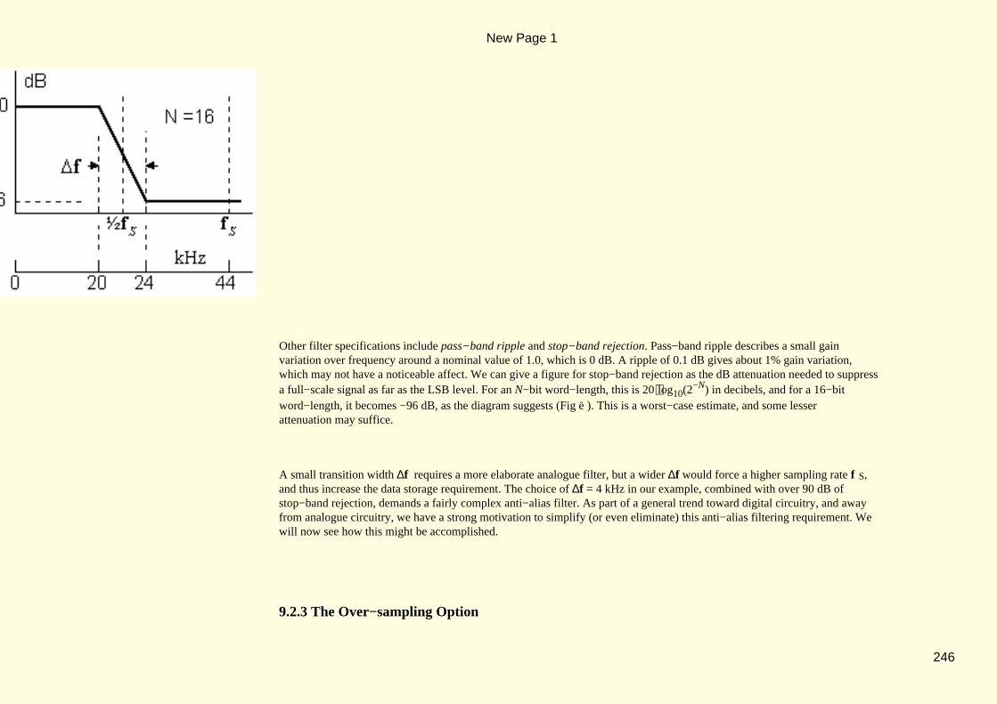
Other filter specifications include pass−band ripple and stop−band rejection. Pass−band ripple describes a small gainvariation over frequency around a nominal value of 1.0, which is 0 dB. A ripple of 0.1 dB gives about 1% gain variation,which may not have a noticeable affect. We can give a figure for stop−band rejection as the dB attenuation needed to suppressa full−scale signal as far as the LSB level. For an N−bit word−length, this is 20⋅log10(2

−N) in decibels, and for a 16−bitword−length, it becomes −96 dB, as the diagram suggests (Fig ë ). This is a worst−case estimate, and some lesserattenuation may suffice.

A small transition width ∆f requires a more elaborate analogue filter, but a wider ∆f would force a higher sampling rate fS,and thus increase the data storage requirement. The choice of ∆f = 4 kHz in our example, combined with over 90 dB ofstop−band rejection, demands a fairly complex anti−alias filter. As part of a general trend toward digital circuitry, and awayfrom analogue circuitry, we have a strong motivation to simplify (or even eliminate) this anti−alias filtering requirement. Wewill now see how this might be accomplished.

9.2.3 The Over−sampling Option

New Page 1

246

Over−sampling means sampling faster than is necessary. If we double the sampling rate for our audio signal, up from 44 kHzto 88 kHz, we will have an OSR (an Over−Sampling Ratio) of 2. Using the same method as before, the new specification forthe anti−alias filter is as shown (Fig ê ).

We now have a transition band ∆f = 48 kHz in width, up from 4 kHz originally. This will vastly simplify the analogueanti−alias filter, but it also means processing the digital data at twice the rate that is needed. We don’t have to do that. We canactually halve the data rate again by discarding every second sample of our digital data stream, but there is a condition. Beforewe discard any samples, we must digitally filter this data to the original specification, for a stop−band that commences at24 kHz as shown on the diagram. The overall result is that a difficult analogue filtering job has become mostly adigital filtering job. But, this is generally quite acceptable, because the digital filtering can usually be done at little additionalcost.

This OSR of 2.0 is only the beginning. Since the digital circuitry of today runs at speeds that are vastly higher than audiosampling rates, oversampling ratios of several hundred are realizable. These high ratios have become commonplace in"Delta−Sigma"−type A/D converters, and with them the analogue anti−alias filter problem is all but eliminated.

New Page 1

247

9.2.4 Quantization Issues

This diagram shows signal quantization (Fig ç ) as a plot of binary codes versus analogue input voltage, in a range from −1Vto +1V. We've shown a twos complement code with a 3−bit word−length (N = 3). The 45° line shows true analogue levels,for comparison with the stepped code levels, such that the difference between them is the quantization error. This is anillustration of quantization by rounding, which always seeks to minimize the error magnitude. For a step−size q, it gives aquantization error range of ±½q. This error range is also indicated by the small black rectangle symbol on the diagram.

Another option is to quantize by truncation. That means always using the nearest code level that is smaller than the signallevel, as this diagram illustrates (Fig ç ). In this case, the quantization error is in a range from 0 to q, and this range isindicated by the small black rectangle symbol. We could have used a twos complement code here too, but we've shown anoffset binary code instead. The only difference is in the toggling of the MSB.

In some instrument applications, we could find sign−magnitude coding, where the MSB is a sign bit (0 for plus and 1 forminus), and the remaining bits count up the magnitude from zero. That would alter the meaning of truncation, as this diagramillustrates (Fig í ). Here, the truncation is in the direction of the horizontal 000 line. The error now ranges from −q to +q, asthe small black symbol indicates.

Quantization errors are constrained to the ranges that we indicated and, within those ranges, their sample−to−samplevariations are mostly random. Later on, we'll use this information to characterize the noise in terms of its mean noise power.

New Page 1

248

One thing we can say right away : if the word length is reduced by one bit, then the step−size q is doubled, the quantizationnoise level is doubled, and the mean noise power is quadrupled. In decibels, that's a 6 dB increase in noise−power for a 1−bitreduction in word length.

We can use simulation methods and a random number generator to investigate quantization effects in a system. For thatpurpose, we also need functions that can quantize a signal in the ways that we have illustrated. Such functions are easilydefined in Mathcad and in MATLAB.

New Page 1

249

9.3 DIGITAL TO ANALOGUE (D/A) CONVERSION

The sections deals with D/A conversion from a signals perspective. We are not concerned with the technology of D/Aconversion, only with the effects on the signal itself, with emphasis on the faithful re−construction of a band−limited signalx(t) from its samples x(nT).

9.3.1 A Re−construction Model

We will now describe the conversion of a signal from a number−sequence in a computer (or DSP chip) into a continuousanalogue output signal, with the help of a D/A converter. Part (a) below (Fig ê ) depicts the signal as x(nT), the samplednumeric form, as it exists before D/A conversion. The numbers are represented as impulses, and the impulse strengths are thenumeric data values. On the right, we see the band−limited periodic spectrum of this data sequence. Because we consider the

numbers to be value−samples of x(t), the correct spectral description is the scaled X(f)~/T, rather than just X(f)~.

A D/A converter will convert samples sequentially, and will hold the current sample value until the next sample comes along.Stated otherwise, it interpolates between samples using a zero−order hold (or ZOH) operation, and the result is the steppedwaveform xo(t) in part (c) of the diagram. This falls far short of the ideal sinc interpolation that would restore the true x(t). It'snot practical to attempt a sinc interpolation, but we can bring xo(t) much closer to x(t) by doing a little analogue filtering of theD/A converter output. Before that, it will help if we understand in spectral terms what the zero−order hold does to the signal.

New Page 1

250

That is the purpose of part (b) in the diagram. It shows a pulse Π(t/T) of width T and height 1.0. If we convolve this pulse withan impulse of strength x(nT), we get a copy of the pulse adjusted to a new height of x(nT). This action converts an impulse to azero−order hold value, and holds it for T seconds. Consequently, convolution of the impulses x(nT) in part (a) with Π(t/T) inpart (b) will generate the DAC output signal xo(t) of part (c). This will now enable us to see how the spectrum is altered byD/A conversion.

New Page 1

251

Using the scaling property of the CFT, the spectrum of Π(t/T) becomes T⋅sinc(fT). The right side of (b) shows this as a

spectral magnitude plot, as |T⋅sinc(fT)|. We know that convolution in time equates to spectral multiplication, and therefore thespectrum of xo(t) must be :

This ignores a small T/2 time delay which causality implies, but which has little effect. Because the output xo(t) is ananalogue signal, it spectrum Xo(f) is not periodic. Multiplication by the sinc has accomplished this. The "ideal" Xo(f) would be

X(f), the CFT of x(t), which is also an exact copy of the base−band period of X(f)~, with all of its images reduced to zero.

(That is what we would get from a true sinc−t interpolation). The reality is the Xo(f) of part (c), with significant shortcomings,as follows.

The shaded region here (Fig ç ) is the sinc− baseband area, and it shows clearly how the higher baseband frequencies areattenuated by the ZOH action. At the top of the signal band, the reduction is by sinc(½) = 0.637, that's a 36 % reduction atthe high end. In practice, this is easily remedied before D/A conversion, by use of a digital filter that amplifies the higherfrequencies, in anticipation of this effect. The filter spectrum would look something like this (Fig ç ). Analogue outputdevices, including audio−CD players, use this kind of compensation.

New Page 1

252

The other problem with Xo(f) is the inadequate suppression of image frequencies, as shown in the encircled area here (Fig í ).This can be remedied by analogue post−filtering, after D/A conversion. We've also shown the outline of an analogueanti−image filter that would suppress the image but leave the base−band undisturbed. It requires a narrow transition band,which could result in a moderately complex analogue filtering task that we would very much like to avoid. If fact, we canagain turn to over−sampling methods to turn this analogue task into a digital one.

9.3.2 The Over−sampling Option

Quite often, the digital information is available at the normal rate, it is not oversampled. As an example, the audio data on aCD is at 44.1 kHz (because higher rates would take up too much space). So how can we over−sample ?

The answer is to interpolate the available data, and we've already seen how to do this using the DFT (ï Ch 6.3.4), but we canalso do it by other methods. To increase the sample−rate by U = 4, we would first insert 3 zeros between adjacent samplepairs, and then send this 4−times expanded sequence through a low−pass digital filter. The filter output is the 4−timesoversampled signal that we require. We'll describe this technique in much greater detail later. For now, it's sufficient to knowthat we can easily increase the sample rate by an integer ratio of our choosing, and then send the up−sampled data to the D/A

New Page 1

253

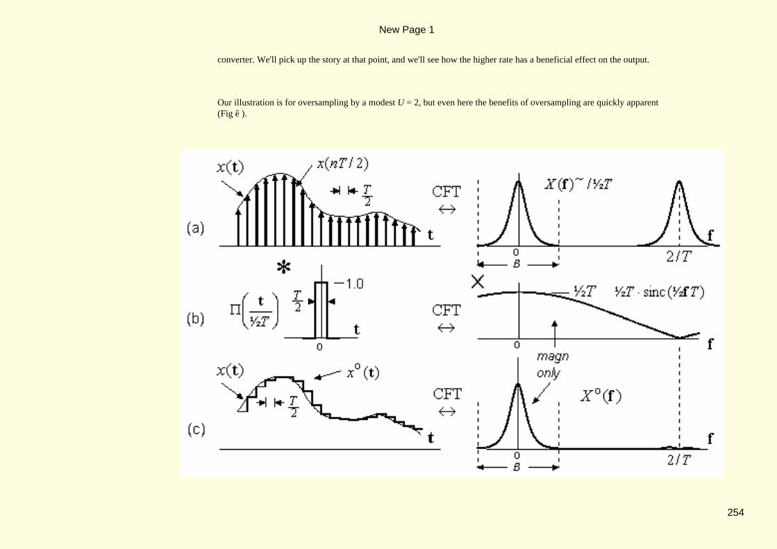
converter. We'll pick up the story at that point, and we'll see how the higher rate has a beneficial effect on the output.

Our illustration is for oversampling by a modest U = 2, but even here the benefits of oversampling are quickly apparent(Fig ê ).

New Page 1

254

We've used spectral symmetry to save space by showing only a little of the negative−frequency part. The new sample intervalis T/2, but the base−band width is unchanged at a (double−sided) value of B =1/T, as shown on the diagram. The images aremoved out to 2/T and beyond, and this simplifies the post−filtering requirement in two ways. First, the anti−image analoguefilter can have a very wide transition band. Second, the image in Xo(f) at 2/T is already smaller than before, and this toorelaxes the filter specification. We can see the improvement more intuitively in the time−domain plot (c), where the steppedoutput signal is already closer than before to the x(t) that we want as our end−product.

Higher values of U will give further improvement, with less need for analogue anti−image filtering, as for example in a CDplayer labelled "8 × oversampling". Nowadays, far higher values of U, coupled with Delta−Sigma noise shaping, give us asolution that is almost totally digital. Delta−Sigma methods are another topic that we will take up in a later chapter.

New Page 1

255

9.4 WINDOWING AND ITS EFFECTS

If we multiply a signal x(t) by Π(t/W), a unit−height rectangular pulse of width W seconds, we retain that part of x(t) in therange (−½W < t < ½W), and we set the rest to zero (Fig í ). It’s equivalent to using a copy of x(t) that ignores everythingoutside the "window" formed by Π(t/W). In DSP we call it "windowing", it is something that we do frequently, and for variousreasons. It may be because the available x(t) data is less than complete, or because we can speed the work by neglecting thefar−out parts that tail off gradually to zero. In some cases, the x(t) is a theoretical shape that goes on forever (such as the sinc),but when we use it in computations we must limit the work−load by ignoring its outer regions. Whatever the reason forwindowing, it amounts to an obvious distortion of a signal in time domain, whereas it is less obvious but may still be quiteserious in the spectral domain. We need to understand the implications of windowing, and we must often take correctiveaction as well.

New Page 1

256

9.4.1 Rectangular Windowing

Windowing with Π(t/W) ( pronounced "rect of t/W ") is called Rectangular windowing. In practice, we would useΠ((t − t 0)/W) for a window that is centered on t0, so that we can place it where we please. But, to understand windowing,we'll find it easier to avoid the linear phase terms caused by time−shifting, so we'll continue to use Π(t/W) for its real and evenspectrum, which is W⋅sinc(Wf). There is no phase term to worry about, and it looks like this (Fig ê ).

Because the "window" is a Π(t) that's been stretched by W, then, by the CFT scaling property, this spectrum is a sinc(f) thathas been compressed, and made taller, by the same factor W. The shaded part known as the "main−lobe" is of height W, and ofwidth 2/W, that is two lobes wide. The main−lobe area is slightly over 1.0 and, if we let W → ∞, it approaches true impulsiveshape. To the left and right of the main−lobe we have "side−lobes" that oscillate and decay, inside a 1/f envelope extending allthe way to infinity.

We'll use a windowed cosine to see what windowing does to a spectrum. A cosine goes on forever, and the spectrum of thecosine signal cos(2πf1t) is a pair of impulses of strength ½ located at ±f1, as seen below (Fig ê ). The windowed cosine isx(t) = cos(2πf 1t)⋅Π(t/W), and is shown here (Fig ç ) for f1 = 2 and W = 3, that is, for a 2 Hz cosine in a 3−secondwindow. The effect of windowing on the cosine spectrum is to convolve it with the window spectrum, yielding:

New Page 1

257

This generates two copies of the sinc, one at −f1, another at +f1, and both scaled by the impulse strength of ½. The spectrumbecomes:

This is the X(f) in the diagram (Fig ê ), and it replaces the impulsive spectrum of an un−windowed cosine. It shows tallnarrow pulses at the ±2 Hz phasor frequencies, and a lot of smaller oscillations elsewhere.

New Page 1

258

The new X(f) tries to approximate the pair of impulses, and it does a better job as the window is made wider. As W→ ∞, thetwo main−lobes approach impulse shape, each with a strength close to ½, and the oscillations decay more rapidly as we moveaway from the main−lobe frequencies.

The shortcomings of X(f) are two−fold. The finite main−lobe width limits the spectral resolution to around ∆f = 2/W Hz.It means that on a spectrum of two cosines that are closer in frequency than this ∆f, we will find it difficult to tell them apart.

New Page 1

259

Spectral resolution is inversely proportional to window width W, and we can always make it better by using a wider window,that means using more data, provided the data is available.

The second problem is the side−lobes. They suggest that we have signal content at frequencies where none exists, even atfrequencies far removed from f1. In a signal that has two cosine frequencies, a strong tone and a weak tone, the side−lobesfrom the strong tone could swamp the weak tone altogether, such that we fail to recognise it. The side−lobe content is calledspectral leakage. It is important that we minimise leakage, but reducing leakage is less easy than improving the spectralresolution. Intuitively, leakage describes all the frequencies that are needed to build the sudden steps that occur at the windowedges (Fig ç ). This in turn gives us a clue as to how the leakage can be reduced.

9.4.2 The Hanning Tapered Window

The basic approach to reducing leakage is to use a tapered window, such as this one (Fig í ), in place of the (broken−line)rectangular window. The taper eliminates the sharp edges that make leakage so severe, and we can expect a greatly−reduced

New Page 1

260

leakage effect in return. The price paid is that a tapered window distorts a signal, even inside the window region, but thisdistortion is often less serious in the spectral view than the distortion by rectangular windowing. We will use the same cosinesignal, for a comparison of the spectral effects.

The tapered window in the diagram (Fig ç ) is called a Hanning window, or a raised−cosine window, and it follows thisdescription:

It's just one period of a cosine, of peak value ½, and also raised by ½. When we window our cosine signal in this way, theresult is as shown (Fig ç ), and the spectrum of this tapered cosine looks like this (Fig ê ).

New Page 1

261

For ease of comparison, we've retained the scaling of the rectangular−windowed spectrum. Here, the main lobes are half astall and twice as wide, with a main−lobe area that is again close to ½. The greater main−lobe width halves the spectralresolution, but we can usually compensate for this unwelcome effect by using a wider time window. More importantly, theside lobes have been greatly reduced (in confirmation of our intuitive reasoning). The major benefit of a tapered window isthis reduced spectral leakage.

New Page 1

262

9.4.3 Hanning versus Hamming

The Hanning window is just one of many tapered windows that we can choose from. Although the windowed cosine was auseful example, we can evaluate a window in isolation, with no particular signal in mind. A window w(t) has a spectrum W(f),and we can evaluate the window by inspection of its W(f).

When w(t) = hann(W,t) as given above, we can use the CFT pairs numbered 7 and 9 (ï Ch 8.3.3) to see that it's spectrum is:

This is a convolution of a sinc with three impulses, and the result is a sum of three scaled and shifted copies of the sinc. Itbecomes:

Using a nominal width of W = 1, this spectral diagram shows the three sincs individually (Fig ë ). The next diagram showsthe sum of these sincs, which is the Hanning window spectrum (Fig ç ). The Hanning has low leakage because the sincs adddestructively in side−lobe regions. We've also shown the rectangular window spectrum for comparison. The Hanningmain−lobe is twice as wide, but its side−lobes are very much smaller.

New Page 1

263

The Hamming window is just a small variation on the Hanning:

and

It makes small adjustments in DC level, and in the cosine amplitude, to obtain better suppression of the nearest side−lobes, butthe side−lobes are hard to see on a linear scale. We will use a log scale to make the side lobes more visible, but we don't needto show the negative frequencies.

These (Fig ç ) are dB spectral plots for all three windows. Each plot is adjusted for 0 dB at f = 0. To illustrate this for theHanning window, the function that we have plotted is:

The side−lobes can now be compared. The rectangular window has large side−lobes, the largest being −13.5 dB for thenearest lobe. This compares with −32 dB for the Hanning window and −42 dB for the Hamming window. By thiscomparison, the Hamming window wins, but the Hanning side−lobes are better in the sense that they fall away rapidly with

New Page 1

264

frequency. In practice, the choice of a suitable window will depend on the context in which it is used.

9.4.4 The Blackman Window

The Blackman window achieves even greater side−lobe suppression, using broadly similar methods. It is defined by:

and by

New Page 1

265

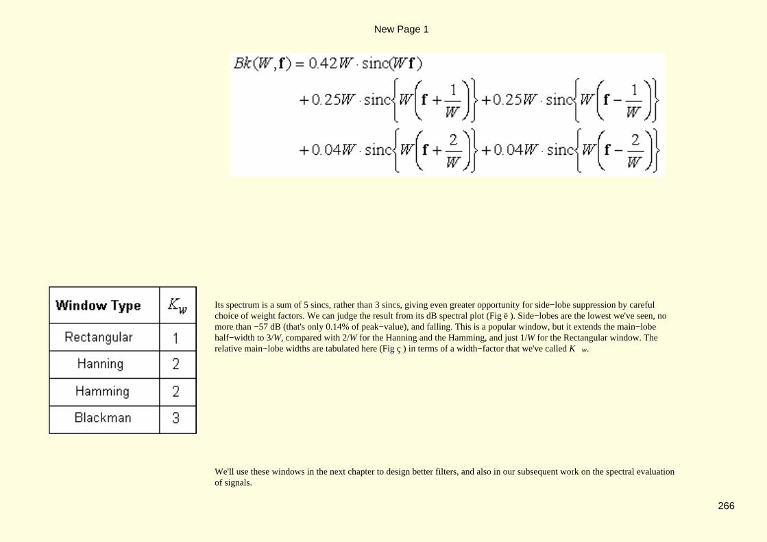
Its spectrum is a sum of 5 sincs, rather than 3 sincs, giving even greater opportunity for side−lobe suppression by carefulchoice of weight factors. We can judge the result from its dB spectral plot (Fig ë ). Side−lobes are the lowest we've seen, nomore than −57 dB (that's only 0.14% of peak−value), and falling. This is a popular window, but it extends the main−lobehalf−width to 3/W, compared with 2/W for the Hanning and the Hamming, and just 1/W for the Rectangular window. Therelative main−lobe widths are tabulated here (Fig ç ) in terms of a width−factor that we've called Kw.

We'll use these windows in the next chapter to design better filters, and also in our subsequent work on the spectral evaluationof signals.

New Page 1

266

New Page 1

267

10.1 PREAMBLE

This chapter shows how we can build an FIR filter that approximates any specified spectral shape. Some important propertiesof FIR filters are identified and discussed. We also commence a gradual move toward a new "z−notation" which will lateracquire more formal status as the z−transform. We show how advanced computer−based algorithms can give betterperformance than our (theoretically simpler) approach, and are also easy to use.

New Page 1

268

10.2 FIR FILTERS FROM FT PAIRS

An LTI filter is specified by its impulse response, h[n], a discrete data sequence. This is a signal description as well as a filterdescription, and no distinction is necessary. The signal spectrum is H(f), and this is also the filter spectrum. Fourier Transform(FT) theory provides the link between signals and their spectra, and forms the basis for the design method that we will present.

10.2.1 Filters based on CFT Pairs

A majority of filters are based on (idealised) brick−wall descriptions, and these are easily derived from CFT pairs. Forexample, a low−pass ((LP) filter with a passband extending from DC to a cut−off frequency fc (in Hz) can be based on theCFT pair shown here (Fig ê ).

New Page 1

269

This (h(t), H(f) pair is a scaled version of CFT pair 5 in our Table (ï Ch 8.3.3). We've stretched Π(f) by 2fc, causingsinc(t) to become narrower and taller by the same factor. The resulting H(f) is the spectrum of an ideal analogue LP filter withcutoff frequency fc Hz, and h(t) is the filter's impulse response. To convert the filter to digital form, we must have a sampling

frequency fS which is suitably higher than 2f

c. We then replicate H(f) at intervals of f

S into a periodic H(f)~ which is the

spectrum of a set of area−samples T⋅h(nT) from h(t), where T = 1/fS. These area−samples become h[n], the coefficients ofour digital LP filter.

Our filter has a two−sided bandwidth of 2fc Hertz. For digital working, we prefer the normalised bandwidth which we'll callb :

b = 2 fc/fS = bandwidth (cycles/sample) [two−sided, normalised]

Remembering that h(t) = 2fc⋅sinc(2fct), our filter coefficients become:

New Page 1

270

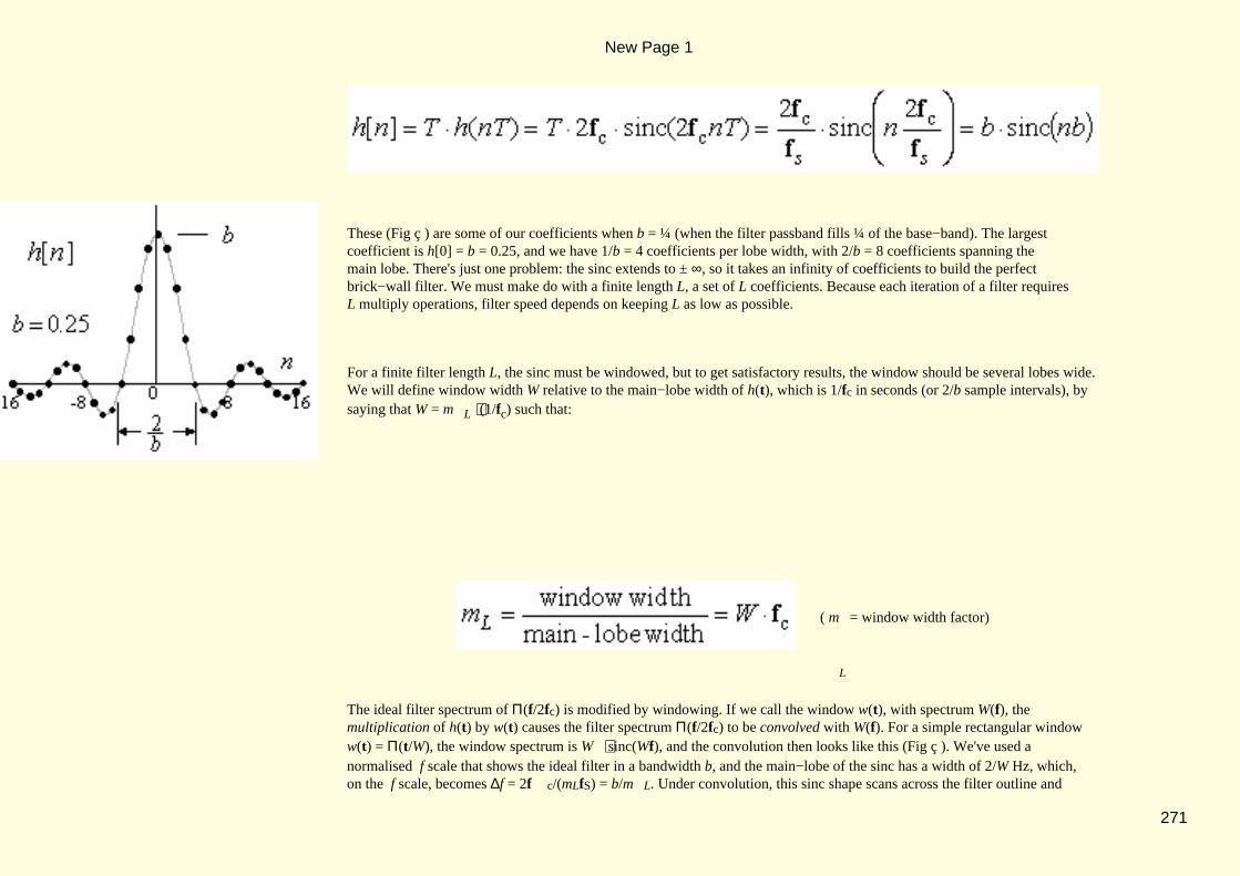
These (Fig ç ) are some of our coefficients when b = ¼ (when the filter passband fills ¼ of the base−band). The largestcoefficient is h[0] = b = 0.25, and we have 1/b = 4 coefficients per lobe width, with 2/b = 8 coefficients spanning themain lobe. There's just one problem: the sinc extends to ± ∞, so it takes an infinity of coefficients to build the perfectbrick−wall filter. We must make do with a finite length L, a set of L coefficients. Because each iteration of a filter requiresL multiply operations, filter speed depends on keeping L as low as possible.

For a finite filter length L, the sinc must be windowed, but to get satisfactory results, the window should be several lobes wide.We will define window width W relative to the main−lobe width of h(t), which is 1/fc in seconds (or 2/b sample intervals), bysaying that W = mL ⋅(1/fc) such that:

( m

L

= window width factor)

The ideal filter spectrum of Π(f/2fc) is modified by windowing. If we call the window w(t), with spectrum W(f), themultiplication of h(t) by w(t) causes the filter spectrum Π(f/2fc) to be convolved with W(f). For a simple rectangular windoww(t) = Π(t/W), the window spectrum is W⋅sinc(Wf), and the convolution then looks like this (Fig ç ). We've used anormalised f scale that shows the ideal filter in a bandwidth b, and the main−lobe of the sinc has a width of 2/W Hz, which,on the f scale, becomes ∆f = 2fc/(mLfS) = b/m L. Under convolution, this sinc shape scans across the filter outline and

New Page 1

271

distorts it. The convolution in the diagram is for mL = 4, indicating a window span that just covers the samples in the h[n]plot above, and that yields a filter length of L = 33. We can view the resulting spectrum as the DtFT taken over thesesamples, that is:

Direct evaluation of this H(f) gives the plot that we see here (Fig ê ). We've shown a range of f that is twice the basebandwidth, just to emphasise the periodicity of H(f), although the range (0 < f < 0.5) would suffice.

New Page 1

272

The result of convolution with the window spectrum W⋅sinc(Wf) is evident in the oscillations that we see. Passband gain

remains close to 1.0 because the area of W⋅sinc(Wf) is 1.0, but the ripple gives considerable variation. Stopband attenuation ispoor, again because of the ripple. ∆ f = b/mL takes on special significance as the width of the transition band, as well asbeing the main−lobe width of W⋅sinc(Wf). We can see why this is so from the spectral convolution caused by windowing(Fig ë ).

We defined the time−window width as mL × (main−lobe width) which, expressed in sample intervals, becomes mL⋅2/b,which is 2/∆ f. This is also the filter length, except that we treat h[0] as one extra coefficient, and therefore:

the filter length

In practice, we round up the value of L to the nearest integer (often to the nearest odd−valued integer). The important point isthat a sharp transition requires a long filter. Filter length is the price that we pay for a narrow transition band, ∆ f.

The ripple is an unwelcome aspect that needs attention. It arises from the sharp cutoff of a rectangular window, and can begreatly reduced by using a tapered window instead. All that we said about tapered windows is applicable here. The spectra oftapered windows have a main lobe that is wider by a factor Kw, as previously defined (ï Ch 9.4.4), and the Table is shownagain here (Fig ç ). The Blackman window has the lowest side−lobes, but it also give the greatest transition width for a givenfilter length. We must now modify our length estimate to read:

New Page 1

273

We'll use the Hamming window to show how coefficient values are altered. The window description is (ï Ch 9.4.3):

and our new set of coefficients becomes:

(−16 < n < 16)

The indexing range shown is for our present example. We've also moved from seconds to sample−intervals by replacingt/W with n/L. The tapered coefficients reduce in value as we move away from centre, like this (Fig ç ). The DtFT of thetapered coefficients gave us this new spectral diagram (Fig ê ).

New Page 1

274

The ripple is much smaller, as expected, but the transition band is wider. Nominally, it is twice as wide, but this is a ratherimprecise measure, and we'll introduce a better measure shortly. For a better appreciation of filter performance, a log scale isrequired, and only the positive baseband need be shown. This is the log plot of H(f) for the same hamming−windowed filter(Fig ç ), and it shows almost 60 dB of stopband rejection. For comparison, this is the corresponding result when a Blackmanwindow is used (Fig í ). The stopband rejection is much better, but the main lobe is wider, although not so wide as ourKw figures would suggest. Notice how the stopband ripple has a period of 1/W Hz, which is ½b/mL on the f scale.

The following is a suitable design procedure:

Choose bandwidth b ( = 2 fc/f1. S), and transition width ∆ f.

New Page 1

275

Choose a window to give the desired attenuation• Choose filter length L close to 1+2 K•

w/ ∆ f, even or odd.Compute coefficients h[n] and spectrum H(f).• Examine H(f) and iterate the solution if required.•

One can use odd−length filters in general, and even−length filters where there is a specific requirement for same.

10.2.2 FIR Filters by Inverse DtFT

In the example just completed, we started with an analogue LP filter based on a CFT pair, and we moved to digital filter formby time−domain sampling. We did this to emphasises the analogue domain connection, but in fact we could have found thesame filter more directly using the DtFT. The key to this approach is the inverse DtFT integral (ï Ch 6.4.1):

normalised IdtFT integral

We just specify the H(f) that we require, and then use this integral to find h[n]. We deal with windowing issues in the sameway as before. To illustrate the method, we will design a brickwall band−pass (BP) filter. The LP filter is a special case of the

New Page 1

276

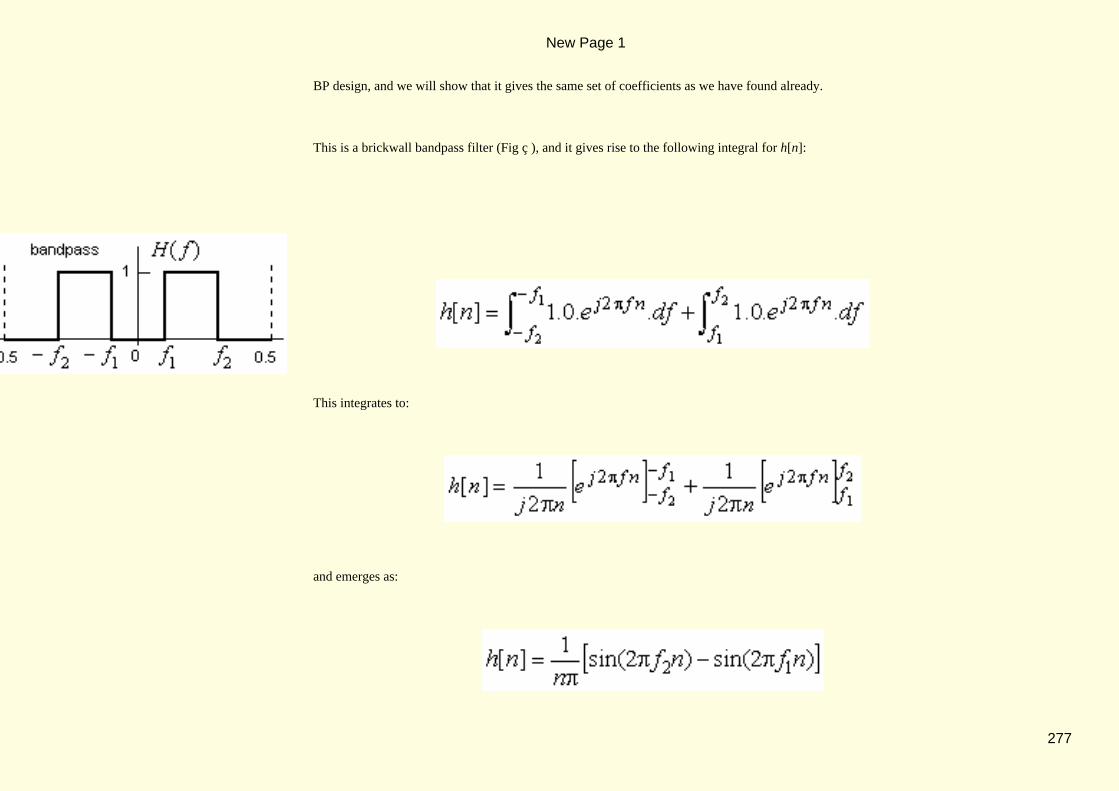
BP design, and we will show that it gives the same set of coefficients as we have found already.

This is a brickwall bandpass filter (Fig ç ), and it gives rise to the following integral for h[n]:

This integrates to:

and emerges as:

New Page 1

277

The case of n = 0 must be integrated separately to yield h[0] = 2(f2 − f 1). We can also write this h[n] in terms of the sincfunction:

We can check the low−pass (LP) case by setting f1 = 0 and f 2 = ½b. It yields h[n] = b.sinc(nb), the same result asbefore. For the high−pass (HP) case, we set f2 = 0.5, (Fig ç ) and the pass−band, which now extends circularly from f1 to−f1, has a width which we can write as b = 1− 2f1. In this case:

and it becomes:

Except for the (−1)n term, this is the same as the LP case. The only difference is that coefficients at odd values of n changesign.

New Page 1

278

We can now obtain coefficients for a brickwall filter of any specification. There is still the matter of ripple, and oftransition−band width, and those issues are dealt with in the same way as before. But we are not restricted to brickwall filters.We can specify any H(f) in the IdtFT integral. Quite often, the integral is an easy one, and we get an algebraic expression forh[n]. In more difficult cases, we can use numeric integration, and still get a result. We can even specify the desired H(f) as aset of DFT spectral values, and then use the IDFT to get the desired h[n], but we should note the possibility of time−domainaliasing if we use this approach.

10.2.3 Differentiators by Inverse DtFT

A filter that differentiates a signal is very different from the brickwall type, and we'll use it as a further illustration of theIDtFT method. The output from such a filter should approximate the slope of the input signal. We may be familiar with theanalogue case, where an input signal x(t) is differentiated to give an output y(t) = dx(t)/dt, and the filter spectrum isH(f) = j2πf, or simply jω. To build a simple digital differentiator, we can approximate this action as:

differentiation

Substituting f = f/f S = fT, it becomes (x[n] − x[n−1]) ↔ j2πf. The filter that gives y[n] = x[n] − x[n−1] has animpulse response h[n] = 1 −1, and we will soon show that its spectrum H(f) is a good approximation to j2πf at lowfrequency (below f = ¼).

The more formal way to design a differentiator is to set H(f) = j2πf and insert this in the IdtFT integral. Since all H(f) areperiodic in (−0.5 < f < 0.5), we can use these ±0.5 limits, but we may prefer a lower limit f0 as suggested here (Fig ç ).Using this in the IdtFT integral, we must find:

New Page 1

279

We can apply the known integral:

with a = j2πn and, after some algebra, we get the result:

New Page 1

280

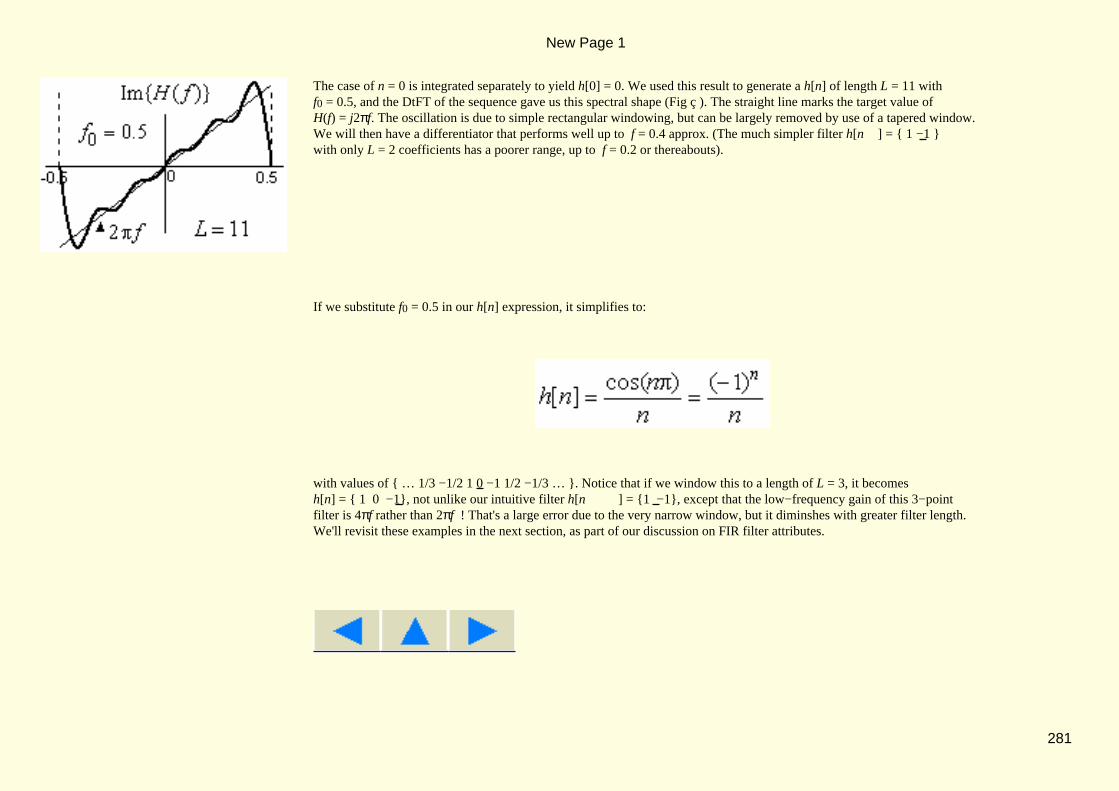
The case of n = 0 is integrated separately to yield h[0] = 0. We used this result to generate a h[n] of length L = 11 withf0 = 0.5, and the DtFT of the sequence gave us this spectral shape (Fig ç ). The straight line marks the target value ofH(f) = j2πf. The oscillation is due to simple rectangular windowing, but can be largely removed by use of a tapered window.We will then have a differentiator that performs well up to f = 0.4 approx. (The much simpler filter h[n] = 1 −1 with only L = 2 coefficients has a poorer range, up to f = 0.2 or thereabouts).

If we substitute f0 = 0.5 in our h[n] expression, it simplifies to:

with values of … 1/3 −1/2 1 0 −1 1/2 −1/3 … . Notice that if we window this to a length of L = 3, it becomesh[n] = 1 0 −1, not unlike our intuitive filter h[n ] = 1 −1, except that the low−frequency gain of this 3−pointfilter is 4πf rather than 2πf ! That's a large error due to the very narrow window, but it diminshes with greater filter length.We'll revisit these examples in the next section, as part of our discussion on FIR filter attributes.

New Page 1

281

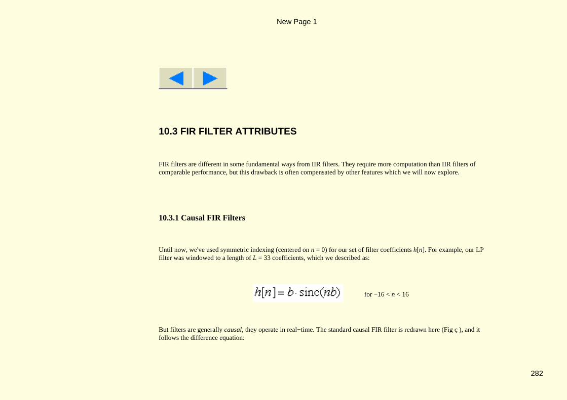
10.3 FIR FILTER ATTRIBUTES

FIR filters are different in some fundamental ways from IIR filters. They require more computation than IIR filters ofcomparable performance, but this drawback is often compensated by other features which we will now explore.

10.3.1 Causal FIR Filters

Until now, we've used symmetric indexing (centered on n = 0) for our set of filter coefficients h[n]. For example, our LPfilter was windowed to a length of L = 33 coefficients, which we described as:

for −16 < n < 16

But filters are generally causal, they operate in real−time. The standard causal FIR filter is redrawn here (Fig ç ), and itfollows the difference equation:

New Page 1

282

The output cannot precede the input, and this means that indexing cannot start before n = 0. The b−coefficients (not to beconfused with bandwidth b) are just the h[n] values, but the indexing is different. In our LP filter example:

for n = 0,1,2 .. 32

The only difference between bn and h[n] is a right−shift, or a time delay, of the h[n] sequence by 16 samples, which is½(L −1) samples in the general case.

10.3.2 The Linear Phase Attribute

Most of our FIR filters have important symmetries. A glance at the LP filter coefficients (Fig ç ) shows that they haveeven symmetry, that is:

New Page 1

283

even symmetry

In fact, this is true of the BP and HP filters as well. If we turn to the differentiator example, we find that it has odd symmetry,that is:

and odd symmetry

A majority of FIR filters have one or other of these symmetries, with important consequences for the filter spectrum, asfollows. When we compute the spectrum by DtFT, the coefficients (except for h[0]) combine naturally in pairs. For a filter oflength L = 3, we have:

For the even−symmetry case, h[−1] = h[1], and then:

The notable thing about this H(f) is that it is real−valued. For the odd−symmetry case, h[0] = 0 and h[−1] = −h[1], and theresult is very different:

New Page 1

284

The notable thing about this H(f) is that its value is imaginary. As we add more coefficient pairs h[−2], h[2], h[−3], h[3]etc, these H(f) continue to be real for even−symmetry filters and imaginary for odd−symmetry filters.

When we go from symmetric indexing to causal indexing, we delay the filter response by ½(L −1) samples. This applies alinear−phase lag term to H(f):

d = ½(L −1) sample intervals

For an even−symmetry filter, H(f) has zero phase at first, and when we make it causal, the linear−phase lag becomes its onlyphase term. It has linear phase, and this brings us to the question of distortion.

A brickwall filter removes certain frequencies from a signal, and tries to leave the remaining part undistorted. But it can stillbe distorted in two ways. If the gain magnitude varies across the passband, this imposes an amplitude distortion on the signal.We saw a ripple effect that could distort in this way, but we were able to minimise it by using tapered windows. The otherkind of distortion is phase distortion. If the phase of H(f) varies linearly over frequency, it delays all frequencies by the sameamount, but that does not change the signal shape, it does not cause phase distortion. If the phase of H(f) in the passband isnon−linear over frequency, then different frequencies will be delayed by different amounts, and the signal will suffer fromphase distortion.

The even−symmetry filter has only a linear−phase lag term, causing it to delay all frequencies equally by ½(L −1) samples, orby ½(L −1)T seconds. This is just the time difference between symmetric and causal responses, and it does not cause phasedistortion. That is one of the big advantages that FIR filters can offer, all the more so because we will see that IIR filtersdo cause phase distortion, and to a degree that is often unacceptable.

New Page 1

285

Odd−symmetry filters do not have strict linear phase, but they have a phase plot that consists of straight−line segments, sothey do have linear−phase slope. That's not enough to eliminate shape distortion in general, but we'll see later that it is asufficient protection for bandpass signals. That makes odd symmetry a useful property also, in some situations. We will soonsee sample spectra to illustrate both linear phase and linear phase slope. Our final task in this section will be to show how wecan ensure that these important symmetries are preserved.

FIR filters having even or odd symmetry are based on a windowed time response:

in which the window function w(t) has even symmetry, and the filter function h(t) has either even or odd symmetry. Theresulting hw(t) has the same symmetry as h(t). We want to maintain this symmetry in the samples from hw(t) that become ourfilter coefficients. For a filter of length L, we will use a window of length W = LT seconds, for both even−length andodd−length filters.

The odd−length case is illustrated here (Fig ç ) when L = 5. The samples include a central value when t = 0, and thesequence is symmetric about the central value. To obtain the causal coefficients bn, we must slide hw(t) to the right by½(L −1) samples, or 2 samples in this case. The samples now commence at t = 0, and we can sample at instants t = nT forn = 0 .. 4. We then get:

n = 0 .. L −1

New Page 1

286

The even−length case is illustrated here (Fig ç ) for L = 4. To maintain symmetry, samples are offset from t = 0 by ±½T.There are 4 samples, forming 2 symmetric pairs. To obtain the causal coefficients bn, we must slide hw(t) to the right by½(L −1) samples, or 1½ samples in this case. The samples now commence at t = 0, and we can sample at instantst = nT for n = 0 .. 3. We then get:

n = 0 .. L −1

This expression is the same as for the odd−length case, so we can use it to ensure symmetry, irrespective of the filter length.Notice that when L is even, we get a non−integer delay. This carries the inference that an interpolation is being performed,producing output samples that are mid−way in time between the input samples.

10.3.3 Filter Descriptions using "z".

The term e−j2πf appeared several times in the last paragraph. It's cumbersome to write, but it describes something quite simple.It's a linear−phase lag term, the frequency−domain equivalent of a T−second delay, or a 1−sample delay.

New Page 1

287

a 1−sample delay

Not surprisingly then, it appears quite often, and it makes sense to have a simpler notation. The common practice is to define anew parameter z as:

from which a 1−sample delay

We will use the new z parameter to help describe some filters that we know, and we will be surprised at how it lets us seethese filters in an entirely new light. In all cases, the filter spectrum is:

For now, this is just the DtFT using a compact notation. Later on, we'll enlarge the concept and call it the "z−transform". Toget an idea of where this can lead us, we'll apply the new notation to our "intuitive" differentiating filter.

The filter is seen here (Fig ç ) and, from its impulse response h[n] = 1 −1, the spectrum is easily found:

New Page 1

288

We've called it H(z) rather than H(f) because the frequency is expressed solely in terms of z. This H(z) is a polynomial in z.H(z) goes to zero when z = 1 and it goes infinite when z = 0. What we normally say is that H(z) "has a zero" at z = 1 and it"has a pole" at z = 0. In all of this, z is a complex−valued frequency variable. Each value of z is a point on a so−called"z−plane". We can show H(z) pictorially on the z−plane by marking in the pole and zero points.

This is a "pole−zero plot" for our simple differentiator (Fig ç ). We defined z as ej2πf which is the same as 1.0∠(2πf ). Itsvalue is constrained to a magnitude of 1.0, at an angle determined by f. That's the significance of the circle on the diagram. Itcontains all possible values of z as we have defined it. It has a radius of 1.0 centered on z = (0+j0). This "unit−circle" is ourfrequency axis. We've shown the "zero" of H(z) as a small circle at z = 1+j0. We've shown the "pole" of H(z) as an "×" at

z = 0+j0. These two points are all that we need to say that H(z) = K⋅(z −1)/z, but they don't give us a value for K. Thepole−zero plot describes H(z) completely in a pictorial way, except for a scale factor. These plots are a popular way ofdescribing digital filters.

This unit−circle plot (Fig ç ) shows baseband frequencies at quadrant points. The numbers inside the circle are z values at the4 corner points. The numbers outside the circle are corresponding f values, as computed from z = ej2πf by noting that z is avector of length 1.0 at an angle θ such that θ = 2π f. The DC point f = 0 is at co−ordinates (1,0). If we go anti−clockwisefrom DC around the top−half of the circle, we move through the positive base−band range from 0.0 around to 0.25 and finallyto 0.5. The bottom half−circle is the negative baseband range. The ±0.5 points coincide because of the strictly periodic natureof digital signal spectra. If we keep going around the circle we cover the same ground again as we enter the higher imagebands. That's because the images are inseparable from the baseband content, and the unit−circle is an expression of this effect.

New Page 1

289

The pole−zero plot can actually tell us the shape of H(f). This diagram (Fig ç ) shows H(z) = (z−1)/z as a ratio of twovectors which connect the zero and the pole to z, where z is both a unit−length vector and a mobile point on the circle thatrepresents frequency. As we traverse the baseband, z moves around the circle and the vector lengths and vector angles changeaccordingly. We can find the spectral magnitide plot as:

and the angle plot as:

By visualising the motion of z on the circle, we can anticipate the shape of these plots. It's worth taking a few moments to tryand do that now. The alternative is to compute mH as |H(z)| using ej2πf in place of z, as in the expressions above, and similarlyfor aH. The results are shown here (Fig ç ) and they should match your predictions ! This is a uni−polar plot, the kind thatwe would normally get from a computer, but the bi−polar plot shown here (Fig í ) has the very same meaning. We allow themagnitude to be positive or negative, and we adjust the phase plot by ±π radians to compensate. We draw bi−polar magnitudeplots so that they reflect the underlying mathematics. In this case, H(z) = 1 − z−1 and :

New Page 1

290

Here’s how we can separate the magnitude and the phase:

New Page 1

291

from which

and

The bi−polar mH plot was drawn to match the mH(f) result seen here, and then we altered the phase accordingly. This mightnow look like linear phase, but true linear phase is linear through the origin, whereas this phase plot is offset by π/2. It haslinear slope, but is not strictly linear. We saw a phase plot for an averaging filter (ï Ch 7.4.1) and it was strictly linear. Thesame is true of the brickwall filters that we described.

The slope of the phase plot reflects the delay term e−jπf , which describes a delay of ½(L −1) samples, or just a ½−sampledelay. The offset of π/2 is the "j" of the ideal j2πf transfer function. The dotted line on the mH plot marks the ideal2πf response. This differentiator is close to the ideal as far as f = ±0.25, about half of the baseband.

New Page 1

292

10.3.4 FIR Transfer Functions using "z".

We can easily extend our z notation to cover FIR filters in general, according to the difference equation:

We probably think of x[n] as "the nth sample" and of x[n−1] as the one before it, and so forth. But, if consider the action overall time, we can also see x[n] as an entire sequence, and we can see x[n−1] as the same sequence, once delayed. The sequencex[n] has a DtFT spectrum which we can write as:

while the spectrum of x[n−1] is z−1⋅X(z) where z−1 describes the 1−sample delay. In similar fashion, the term z−2 describes a2−sample delay, etc. If the difference equation is valid over all time, we can (by superposition) translate each and every terminto a corresponding spectral function, with this result:

New Page 1

293

The filter Transfer Function (TF) is output/input = Y(z)/X(z), which we like to call H(z), and this becomes:

It may not look much like a spectrum, but we can quickly extract the spectral information and plot it over frequency:

and

(−0.5 < f < 0.5)

The H(z) expression covers FIR filters in general, and we feel prompted to use z−1 in place of T as our symbol for a 1−sampledelay (Fig ç ). But there is not very much new here. This new H(z) is just the DtFT of the bn coefficients (the causal versionof h[n] ), using the z−notation. However, the polynomial form of H(z) is convenient for many purposes, and that includeswhat we're about to do next.

10.3.5 Linear−Phase FIR Zero Patterns

New Page 1

294

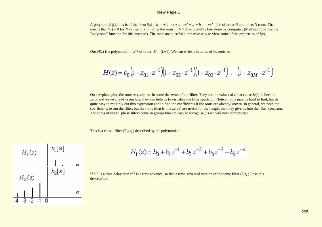
A polynomial f(x) in x is of the form f(x) = b0 + b 1x + b 2x2 + .. + b NxN. It is of order N and it has N roots. Thatmeans that f(x) = 0 for N values of x. Finding the roots, if N > 2, is probably best done by computer. (Mathcad provides the"polyroots" function for this purpose). The roots are a useful alternative way to view some of the properties of f(x).

Our H(z) is a polynomial in z−1 of order M = (L−1). We can write it in terms of its roots as:

On a z−plane plot, the roots z01, z02, etc become the zeros of our filter. They are the values of z that cause H(z) to becomezero, and we've already seen how they can help us to visualise the filter spectrum. Notice, roots may be hard to find, but itsquite easy to multiply out this expression and to find the coefficients if the roots are already known. In general, we need thecoefficients to run the filter, but the roots (that is, the zeros) are useful for the insight that they give us into the filter spectrum.The zeros of linear−phase filters come in groups that are easy to recognise, as we will now demonstrate.

This is a causal filter (Fig ç ) described by the polynomial :

If z−1 is a time delay then z+1 is a time advance, so that a time−reversed version of the same filter (Fig ç ) has thisdescription:

New Page 1

295

H1(z) is a polynomial in z−1. There are 4 values of z−1 that make H1(z) = 0. H 2(z) is a polynomial in z with thesame coefficients. The same 4 numbers, when used as values of z, will make H2(z) = 0. This means that the set of zeros forH1(z) and the set of zeros for H2(z) are at reciprocal locations on the z−plane. We admit that H2(z) is not causal, but that iseasily remedied. A 4−sample right−shift makes it causal, and its spectrum becomes z−4⋅H2(z), but this does nothing to alter itszero locations. It follows that if we alter an FIR filter by reversing the order of its coefficients, then the zeros of the filter willmove to reciprocal locations on the z−plane. We will now apply this idea to a linear−phase filter.

Linear phase comes from coefficient symmetry. If we time−reverse an even−symmetry set of coefficients, we end up with thesame set as we started with (except for a time shift). This implies that reciprocation of the filter zeros has no overall effect ontheir placement. Only certain groups of zeros can meet this condition, primarily the group that we see here (Fig í ).

We have a group of 4 zeros labelled A, B, C, D. They are placed at angles ±θ and at radii of r ( < 1) and 1/r. The zero at A, forexample, is at r∠θ and, when we reciprocate it, we get 1/( r∠θ) = (1/r)∠−θ, which is where D is located. The special propertyhere is that when we reciprocate A it moves to D and when we reciprocate D it moves to A, and similarly for the (B,C) pair.Overall, these points just trade places, and we end up with the same set of zeros as we had before reciprocation. These zerossatisfy the linear−phase condition, but there are other special cases that we can include also. They are all shown here (Fig ê ).

New Page 1

296

The general case is the (a) plot. Plot (b) shows two zeros at 1.0∠±θ. Plot (c) shows real zeros at r and at 1/r. Plot (d) showsreal zeros at −r and at −1/r. Plot (e) has a zero at 1.0. Plot (f) has a zero at −1.0. Its easy to see that they all reciprocate withoutchanging the overall zero placement. A linear−phase filter of length L has L −1 zeros, often quite a large number, and thesezeros can exist as any combination of the groupings in the diagram above. The same applies to filters that have onlylinear−phase slope, because time−reversal of an odd−symmetry sequence involves only a change of sign, and a possible timeshift.

New Page 1

297

The zeros of an averaging filter are all on the unit circle, so they belong in the category of plot (b) above. When the zeros fallon the unit circle, the frequency response H(f) goes to zero at the frequencies that those zeros represent.

New Page 1

298

New Page 1

299

New Page 1

300

New Page 1

301

New Page 1

302

New Page 1

303

New Page 1

304

New Page 1

305

New Page 1

306

New Page 1

307