dr2

Quantum Mechanics as Quantum

Information

(and only a little

more)

Christopher A.Fuchs

Computing Science Research Center

Bell Labs, Lucent Technologies

Room 2C-420, 600–700 Mountain Ave.

Murray Hill,New Jersey 07974, USA

Abstract

In this paper, Itry once again to cause somegood-natured trouble. The issue remains, when willweever stop burdening the taxpayer with conferences

devoted to the quantum foundations? The suspicion is

expressed that no end will be in sight until a means is

found to reduce quantum theory to two or three

statements of crisp physical (rather than abstract,

axiomatic) significance. Inthis regard, no tool appears

better calibrated for a direct assault than quantum

information theory. Far from a strained application of

the latest fad to a time-honored problem, this method

holds promise precisely because a large part—but not

all—of the structure of quantum theory has always

concerned information. It is just that the physics

community needs reminding.

This paper, though taking quant-ph/0106166 asits core, corrects one mistake and offers sev-eral

observations beyond the previous version. In

particular, Iidentify one element of quantum

mechanics that Iwould not label a subjective term

in the theory—it is the integer parameter D

traditionally ascribed to a quantum system via its

Hilbert-space dimension.

1 Introduction1

Quantum theory as a weather-sturdy

structure has been with us for 75 years now.Yet, there is a sense inwhich the struggle for its

construction remains. Isay this because one cancheck that not a year has gone by in the last 30

when there was not a meeting or conference

devoted to some aspect of the quantum

foundations. Our meeting in V¨ axj¨ o, “Quantum

Theory: Reconsideration of Foundations,” is only

one ina long, dysfunctional line.

But how did this come about? What is the

cause of this year-after-year sacrifice to the

“great mystery?” Whatever it is, it cannot be

for want of a self-ordained solution: Go to anymeeting, and it is like being ina holy city ingreat

tumult. You will find all the religions with all

their priests pitted inholy war—the Bohmians [3],the Consistent Historians [4], the

Transactionalists[5], the Spontaneous Collapseans

[6],the Einselectionists [7],the Contextual

Objectivists [8], the outright Everettics [9, 10],

and many more beyond that. They all declare to

see the light, the ultimate light. Each tells us that

if we will accept their solution as our savior,

then we too will see the light.

1This paper, though substantially longer, should be

viewed as a continuation and amendment to Ref. [1].

Details of the changes canbe found inthe Appendix to the

present paper, Section 11.Substantial further arguments

defending a transition from the “objective Bayesian”

stance implicit in Ref. [1] to the “subjective Bayesian”

stance implicit here canbe found inRef. [2].

1

AFraction of the Quantum Foundations Meetings since 1972

1972 The Development of the Physicist’s Conception of Nature, Trieste, Italy

1973 Foundations ofQuantum Mechanics and Ordered Linear Spaces,

Marburg, Germany

1974 Quantum Mechanics, aHalf Century Later, Strasbourg, France

1975 Foundational Problems inthe Special Sciences, London, Canada

1976 International Symposium onFifty Years of the Schr¨ odinger Equation,

Vienna, Austria

1977 International School of Physics “Enrico Fermi”, Course LXXII:

Problems inthe Foundations ofPhysics, Varenna, Italy

1978 Stanford Seminar onthe Foundations ofQuantum Mechanics, Stanford, USA

1979 Interpretations and Foundations ofQuantum Theory, Marburg, Germany

1980 Quantum Theory and the Structures of Time andSpace, Tutzing, Germany

1981 NATO Advanced Study Institute onQuantum Optics, Experimental

Gravitation, and Measurement Theory, BadWindsheim, Germany

1982 The Wave-Particle Dualism: aTribute toLouis deBroglie, Perugia, Italy

1983 Foundations ofQuantum Mechanics inthe Light of New Technology,

Tokyo, Japan

1984 Fundamental Questions inQuantum Mechanics, Albany, New York

1985 Symposium onthe Foundations ofModern Physics: 50Years of

the Einstein-Podolsky-Rosen Gedankenexperiment, Joensuu, Finland

1986 New Techniques andIdeas inQuantum Measurement Theory, New York, USA

1987 Symposium onthe Foundations ofModern Physics 1987: TheCopenhagen

Interpretation 60Years after the Como Lecture, Joensuu, Finland

1988 Bell’s Theorem, Quantum Theory, and Conceptions of the Universe,

Washington, DC,USA

1989 Sixty-two Years ofUncertainty: Historical, Philosophical and

Physical Inquiries intotheFoundations of Quantum Mechanics, Erice, Italy

1990 Symposium onthe Foundations ofModern Physics 1990: Quantum Theory of

Measurement and Related Philosophical Problems, Joensuu, Finland

1991 Bell’s Theorem and the Foundations ofModern Physics, Cesena, Italy

1992 Symposia ontheFoundations of Modern Physics 1992: The Copenhagen

Interpretation andWolfgang Pauli, Helsinki, Finland

1993 International Symposium onFundamental Problems inQuantum Physics,

Oviedo, Spain

1994 Fundamental Problems inQuantum Theory, Baltimore, USA

1995 The Dilemma ofEinstein, Podolsky and Rosen, 60Years Later, Haifa, Israel

1996 2nd International Symposium onFundamental Problems inQuantum Physics,

Oviedo, Spain

1997 Sixth UK Conference onConceptual and Mathematical Foundations of

Modern Physics, Hull, England

1998 Mysteries, Puzzles, and Paradoxes inQuantum Mechanics, Garda Lake, Italy

1999 2nd Workshop onFundamental Problems inQuantum Theory, Baltimore, USA

2000 NATO Advanced Research Workshop onDecoherence anditsImplications

inQuantum Computation and Information Transfer, Mykonos, Greece

2001 Quantum Theory: Reconsideration of Foundations, V¨ axj¨ o,Sweden

But there has to be something wrong with

this! If any of these priests had truly shown the

light, there simply would not be the

year-after-year conference. The verdict seemsclear enough: If we— i.e., the set of people who

might be reading this paper—really care about

quantum foundations, then it behooves us as acommunity to ask why these meetings arehappening and find away to put astop to them.

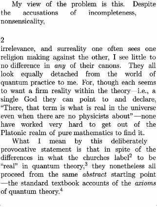
My view of the problem is this. Despite

the accusations of incompleteness,

nonsensicality,

2

irrelevance, and surreality one often sees onereligion making against the other,Isee little to

no difference inany of their canons. They all

look equally detached from the world of

quantum practice to me. For, though each seemsto want a firm reality within the theory—i.e., asingle God they can point to and declare,

“There, that term is what is real inthe universe

even when there are no physicists about” —none

have worked very hard to get out of the

Platonic realm of pure mathematics to find it.

What Imean by this deliberately

provocative statement is that in spite of the

differences in what the churches label 2 to be

“real” in quantum theory, 3 they nonetheless all

proceed from the same abstract starting point

—the standard textbook accounts of the axioms

of quantum theory. 4

The Canon forMost of the Quantum Churches:

The Axioms (plain and simple)

1. For every system, there isa complex Hilbert space H.

2. States of the system correspond to projection operators onto H.

3. Those things that are observable somehow correspond to the

eigenprojectors of Hermitian operators.

4. Isolated systems evolve according to the Schr¨ odinger equation....“But what nonsense is this,” you must be asking. “Where else could they start?” The main issue

is this, and no one has said it more clearly than

Carlo Rovelli [11].Where present-day quantum-

foundation studies have stagnated inthe stream

of history is not so unlike where the physics of

length contraction and time dilation stood before

Einstein’s 1905 paper onspecial relativity.

The Lorentz transformations have the namethey do, rather than, say, the Einstein

transforma- tions, for good reason: Lorentz had

published some of them as early as 1895. Indeed

one could say that most of the empirical

predictions of special relativity were inplace well

before Einstein came onto the scene. But that was

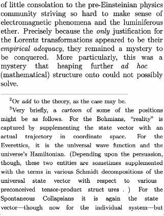
of little consolation to the pre-Einsteinian physics

community striving so hard to make sense of

electromagnetic phenomena and the luminiferous

ether. Precisely because the only justification for

the Lorentz transformations appeared to be their

empirical adequacy, they remained a mystery to

be conquered. More particularly, this was amystery that heaping further ad hoc

(mathematical) structure onto could not possibly

solve.

2Oradd tothe theory, as the case may be.

3Very briefly, a cartoon of some of the positions

might be as follows. For the Bohmians, “reality” is

captured by supplementing the state vector with an

actual trajectory in coordinate space. For the

Everettics, it is the universal wave function and the

universe’s Hamiltonian. (Depending upon the persuasion,

though, these two entities are sometimes supplemented

with the terms invarious Schmidt decompositions of the

universal state vector with respect to various

preconceived tensor-product struct ures .)For the

Spontaneous Collapsians it is again the state

vector—though now for the individual system—but

Hamiltonian dynamics is supplemented with an objective

collapse mechanism. For the Consistent Historians

“reality” is captured with respect toan initial quantum

state and a Hamiltonian by the addition of a set of

preferred positive-operator valued measures (POVMs)

—they call them consistent sets ofhistories—along witha

truth-value assignment within each of those sets.

4To be fair, they do, each intheir own way, contribute

minor modifications to the meanings of a few words inthe

axioms. But that isessentially where theeffort stops.

3

What was being begged for in the yearsbetween 1895 and 1905 was an understanding

of the origin of that abstract, mathematical

structure—some simple, crisp physical

statements with respect towhich the necessity of

the mathematics would be indisputable.

Einstein supplied that and became one of the

greatest physicists of all time. He reduced the

mysterious structure of the Lorentz

transformations to two simple statements

expressible incommon language:

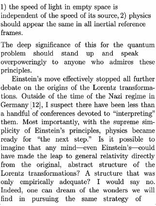
1)the speed of light inempty space is

independent of the speed of its source, 2)physics

should appear the same inall inertial reference

frames.

The deep significance of this for the quantum

problem should stand up and speak

overpoweringly to anyone who admires these

principles.

Einstein’s move effectively stopped all further

debate on the origins of the Lorentz transforma-

tions. Outside of the time of the Nazi regime in

Germany [12],Isuspect there have been less than

ahandful of conferences devoted to “interpreting”

them. Most importantly, with the supreme sim-

plicity of Einstein’s principles, physics became

ready for “the next step.” Is it possible to

imagine that any mind—even Einstein’s—could

have made the leap to general relativity directly

from the original, abstract structure of the

Lorentz transformations? A structure that wasonly empirically adequate? Iwould say no.Indeed, one can dream of the wonders we will

find in pursuing the same strategy of

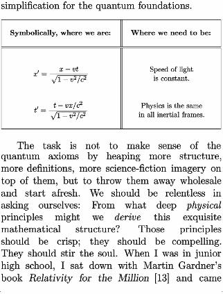
simplification for the quantum foundations.

Symbolically, where we are: Where weneed tobe:

x0 = x − vt

p1− v 2 /c 2

Speed of light

isconstant.

t0 = t− vx/c

2

p1− v 2

/c2

Physics isthe sameinallinertial frames.

The task is not to make sense of the

quantum axioms by heaping more structure,

more defini-tions, more science-fiction imagery ontop of them, but to throw them away wholesale

and start afresh. We should be relentless in

asking ourselves: From what deep physical

principles might we derive this exquisite

mathematical structure? Those principles

should be crisp; they should be compelling.

They should stir the soul. When Iwas injunior

high school, Isat down with Martin Gardner’s

book Relativity for the Million [13] and came

away with an understanding of the subject that

sustains me today: The concepts were strange,

but they were clear enough that Icould get agrasp on them knowing little more mathematics

than simple arithmetic. One should expect noless for a proper foundation to quantum theory.

Until we can explain quantum theory’s essenceto a junior-high-school orhigh-school student and

have them walk away with a deep, lasting

memory, we will have not understood a thing

about the quantum foundations.

So, throw the existing axioms of quantum

mechanics away and start afresh! But how to

pro-ceed? Imyself see no alternative but to

contemplate deep and hard the tasks, the

techniques, and the implications of quantum

information theory. The reason is simple, andI

think inescapable. Quantum mechanics has always

been about information. It is just that the

physics community has somehow forgotten this.

4

Quantum Mechanics:

The Axioms and Our Imperative!

States correspond to density Give an information theoretic

operators ρ over a Hilbert space H. reason ifpossible!

Measurements correspond topositive

operator-valued measures (POVMs) Give an information theoretic

Ed onH. reason ifpossible!

His a complex vector space,

not a realvector space, not a Give an information theoretic

quaternionic module. reason ifpossible!

Systems combine according to the tensor

product of their separate vector Give an information theoretic

spaces, HAB = HA ⊗ HB . reason ifpossible!

Between measurements, states evolve

according to trace-preserving completely Give an information theoretic

positive linear maps. reason ifpossible!

By way of measurement, states evolve

(up tonormalization) via outcome- Give an information theoretic

dependent completely positive linear maps. reason ifpossible!

Probabilities for the outcomes

ofameasurement obey the Born rule Give an information theoretic

for POVMs tr(ρEd ). reason ifpossible!

The distillate that remains—the piece of quantum theory with no information

theoretic significance—will beour first unadorned glimpse of “quantum reality.”

Far from being the end of the journey, placing this conception of nature inopen

view willbethe start ofagreat adventure.

This,Isee as the line of attack we should

pursue with relentless consistency: The

quantum system represents something real and

independent of us; the quantum state represents

a collection of subjective degrees of belief about

something to do with that system (even if only

inconnection with our experimental kicks to it).5

The structure called quantum mechanics is about

the interplay of these two things—the subjective

and the objective. The task before us is to

separate the wheat

5“But physicists are,at bottom, anaive breed,

forever trying to come to terms with the ‘world out

there’ by

methods which, however imaginative and refined, involve

in essence the same element of contact as a well-placed

kick.” —B.S.DeWitt andR.N.Graham[14]

5

from the chaff. If the quantum state

represents subjective information, then how

much of its mathematical support structure

might be of that same character? Some of it,

maybe most of it, but surely not allof it.

Our foremost task should be to go to each

and every axiom of quantum theory and give it

an information theoretic justification if we can.Only when we are finished picking off all the

terms (or combinations of terms) that can be

interpreted as subjective information will we be

in a position to make real progress in quantum

foundations. The raw distillate left

behind—minuscule though it may be with respect

to the full-blown theory—will be our first glimpse

of what quantum mechanics is trying to tell usabout nature itself.

Let me try to give a better way to think

about this by making use of Einstein again.

What might have been his greatest achievement

in building general relativity? Iwould say it

was in his recognizing that the “gravitational

field” one feels inan accelerating elevator is acoordinate effect. That is,the “field” inthat caseis something induced purely with respect to the

description of an observer. In this light, the

program of trying to develop general relativity

boiled down to recognizing all the things within

gravitational and motional phenomena that

should be viewed as consequences of ourcoordinate choices. It was in identifying all the

things that are “numerically additional” [15] to

the observer-free situation—i.e., those things that

come about purely by bringing the observer

(scientific agent, coordinate system, etc.) back

into the picture.

This was a true breakthrough. For in

weeding out all the things that can be

interpreted as coordinate effects, the fruit left

behind finally becomes clear to sight: It is the

Riemannian manifold we call spacetime—a

mathematical object, the study of which one canhope will tell us something about nature itself,

not merely about the observer innature.

The dream Isee for quantum mechanics is

just this. Weed out all the terms that have to

do with gambling commitments, information,

knowledge, and belief, and what is left behind

will play the role of Einstein’s manifold. That is

our goal. When we find it, it may be little

more than a minuscule part of quantum theory.

But being a clear window into nature, we maystart to see sights through it we could hardly

imagine before. 6

2 Summary

Isay to the House asIsaid to ministers who have joined

this government,Ihave nothing to offer but blood, toil,

tears, and sweat. We have before us anordeal of the most

grievous kind. We have before us many, many months of

struggle and suffering. You ask, what isour policy?Isay

it istowage war. War with allour might and with allthe

strength God has given us.You ask,what is our aim? I

cananswer inone word. It isvictory.

—Winston Churchill, 1940, abridged

This paper is about taking the imperative in

the Introduction seriously, though it contributes

only a small amount to the labor it asks. Just

as in the founding of quantum mechanics, this

is

6Ishould point out to the reader that inopposition to

the picture of general relativity, where reintroducing the

coordinate system—i.e., reintroducing the

observer—changes nothing about the manifold (it only

tells us what kind of sensations the observer will pick

up),Ido not suspect the same for the quantum world

Here Isuspect that reintroducing the observer will be

more like introducing matter into pure spacetime, rather

than simply gridding it off with a coordinate system.

“Matter tells spacetime how to curve (when matter is

there), and spacetime tells matter how to move (when

matter is there).” [16] Observers, scientific agents, a

necessary part of reality? No.But do they tend tochange

things once they are on the scene? Yes. If quantum

mechanics can tellus something truly deep about nature,I

think itisthis.

6

not something that will spring forth from alone mind inthe shelter of a medieval college. 7

It is a task for a community with diverse but

productive points of view. The quantum

information community is nothing if not that.8

“Philosophy is too important to be left to the

philosophers,” John Archibald Wheeler once said.

Likewise, Iam apt to say for the quantum

foundations.

The structure of the remainder of the paperis as follows. In Section 3 “Why

Information?,” Ireiterate the cleanest

argument Iknow of that the quantum state is

solely an expression of subjective

information—the information one has about aquantum system. It has no objective reality in

and of itself.9 The argument is then refined by

considering the phenomenon of quantum

teleportation[23].

In Section 4 “Information About

What?,” Itackle that very question [24]

head-on. The answer is “the potential

consequences of our experimental interventions

into nature.” Once freed from the notion that

quantum measurement ought to be about

revealing traces of some preex-isting property [25]

(or beable [26]), one finds no particular reasonto take the standard account of measurement (in

terms of complete sets of orthogonal projection

operators) as a basic notion. Indeed quantum

information theory, with its emphasis on the

utility of generalized measurements or positive

operator-valued measures (POVMs) [27] ,suggests one should take those entities as the

basic notion instead. The productivity of this

point of view is demonstrated by the enticingly

simple Gleason-like derivation of the quantum

probability rule recently found by Paul Busch

[28] and, independently, by Joseph Renes and

collaborators [29].Contrary to Gleason’s original

theo-rem[30], this theorem works just as well for

two-dimensional Hilbert spaces, and even for

Hilbert spaces over the field of rational numbers.

In Section 4.1,Igive a strengthened argument

for the noncontextuality assumption in this

theorem. In Section 4.2, “Le Bureau

International des Poids et Mesures `a Paris,” I

start the process of defining what it means—from the Bayesian point of view—to accept

quantum mechanics as a theory. This leads to

the notion of fixing a fiducial or standard

quantum measurement for defining the verymeaning of aquantum state.

In Section 5 “Wither Entanglement?,” I

ask whether entanglement is all it is touted to be

as far as quantum foundations are concerned.

That is, is entanglement really as Schr¨ odinger

said, “the characteristic trait of quantum

mechanics, the one that enforces its entire

departure from classical lines of thought?” To

combat this, Igive a simple derivation of the

tensor-product rule for combining Hilbert spacesof individual systems which takes the structure

of localized quantum measurements as its starting

point. Inparticular, the derivation makes use of

Gleason-like considerations in the

7If you want to know what this means, ask me over a

beer sometime.

8There have been other soundings of the idea that

information and computation theory can tell us something

deep about the foundations of quantum mechanics. See

Refs. [17], [18], [19],and inparticular Ref. [20].

9In the previous version of this paper,

quant-ph/0106166, Ivariously called quantum states

“information” and “states of knowledge” and did not

emphasize so much the “radical” Bayesian idea that the

probability one ascribes to a phenomenon amounts to

nothing more than the gambling commitments one is

willing to make with regard to that phenomenon. To the

“radical” Bayesian, probabilities are subjective all the way

to the bone. Inthis paper,Istart the long process of trying

to turn my earlier de-emphasis around (even though it is

somewhat dangerous to attempt this ina manuscript that

is little more than amodification of analready completed

paper).Inparticular, because of the objective overtones of

the word “knowledge” —i.e., that a particular piece of

knowledge iseither “right” or “wrong” —I try to steer clear

from the term as much as possible in the present version.

The conception working inthe background of this paper is

that there is simply no such thing as a “right and true”

quantum state. Inallcases, aquantum state isspecifically

and only a mathematical symbol for capturing a set of

beliefs or gambling commitments. Thus Inow variously

call quantum states “beliefs,” “states of belief,”

“information” (though, by thisImean “information” in a

more subjective sense than is becoming common in the

quantum information community), “judgments,”

“opinions,” and “gambling commitments.” Believe me,I

already understand well the number of jaws that will

drop from the adoption of this terminology. However, if the

reader finds that this gives him a sense of butterflies inthe

stomach—or fears that Iwill become a solipsist [21] or a

crystal-toting New Age practitioner of homeopathic

medicine[22]—I hope hewillkeep inmind that this attempt

to be absolutely frank about the subjectivity of some of

the terms inquantum theory ispart of a larger program to

delimit the terms that can be interpreted as objective ina

fruitful way.

7presence of classical communication. With the

tensor-product structure established, the verynotion of entanglement follows in step. This

shows how entanglement, just like the standard

probability rule, is secondary to the structure of

quantum measurements. Moreover, “locality” is

built in at the outset; there is simply nothing

mysterious and nonlocal about entanglement.

In Section 6 “Whither Bayes Rule?,” I

ask why one should expect the rule for

updating quantum state assignments upon the

completion of a measurement to take the form

it actually does. Along the way,Igive a simple

derivation that one’s information always

increases onaverage for any quantum mechanical

measurement that does not itself discard

information. (Despite the appearance otherwise,

this is not a tautology!) Most importantly, the

proof technique used for showing the theorem

indicates an extremely strong analogy between

quantum collapse and Bayes’ rule in classical

probability theory: Up to an overall unitary

“readjustment” of one’s final proba-bilistic beliefs

—the readjustment takes into account one’s

initial state for the system as well as one’s

description of the measurement

interaction—quantum collapse is precisely

Bayesian conditional- ization. This in turn gives

more impetus for the assumptions behind the

Gleason-like theorems of the previous two

sections. In Section 6.1, “Accepting Quantum

Mechanics,” Icomplete the process started in

Section 4.2 and describe quantum measurement

inBayesian terms: Aneveryday mea-surement is

any I-know-not-what that leads to anapplication of Bayes rule with respect to one’s

belief about the potential outcome of the

standard quantum measurement.

In Section 7, “What Else is

Information?,” Iargue that, to the extent that

aquantum state is a subjective quantity, so must

be the assignment of a state-change rule ρ → ρd

for describing what happens to an initial

quantum state upon the completion of ameasurement—generally some POVM—whose

outcome is d.In fact, the levels of subjectivity

for the state and the state-change rule must be

precisely the same for consistency’s sake. To

draw an analogy to Bayesian probability theory,

the initial state ρ plays the role of anapriori

probability distribution P(h) for somehypothesis, the final state ρd plays the role of aposterior probability distribution P(h|d), and

the state-change rule ρ → ρd plays the role of

the “statistical model” P(d| h) enacting theand the

transition P(h) → P(h|d). To the extent that all

Bayesian probabilities are subjective—even the

probabilities

P(d|h) of a statistical model—so is the mapping ρ

→ ρd.Specializing to the case that no information

is gathered, one finds that the trace-preserving

completely positive maps that describe quantum

time-evolution are themselves nothing more than

subjective judgments.

InSection 8“Intermission,” Igive aslight

breather to sum up what has been trashed and

where we are headed.

In Section 9 “Unknown Quantum

States?,” Itackle the conundrum posed by

these very words. Despite the phrase’s

ubiquitous use in the quantum information

literature, what can an unknown state be? A

quantum state—from the present point of view,

explicitly someone’s information—must always be

known by someone, if it exists at all. On the

other hand, for many an application inquantum

information, it would be quite contrived to

imagine that there is always someone in the

background describing the system being

measured or manipulated, and that what we aredoing is grounding the phenomenon with

respect to his state of belief. The solution, at

least in the case of quantum-state tomography

[31] ,is found through a quantum mechanical

version of de Finetti’s classic theorem on“unknown probabilities.” This reports work from

Refs. [32] and [33]. Maybe one of the most

interesting things about the theorem is that it

fails for Hilbert spaces over the field of real

numbers, suggesting that perhaps the whole

discipline of quantum information might not be

welldefined inthat imaginary world.

Finally, in Section 10 “The Oyster and

the Quantum,” Iflirt with the most

tantalizing question of all: Why the quantum?

There is no answer here, but Ido not discount

that we are on the brink of finding one. Inthis

regard no platform seems firmer for the leap

than the very existence of quantum cryptography

and quantum computing. The world is sensitive

toour touch.

8

It has a kind of “Zing!” 10 that makes it fly off

in ways that were not imaginable classically.

The whole structure of quantum mechanics—it is

speculated—may be nothing more than the

optimal method of reasoning and processing

information inthe light of such a fundamental

(wonderful) sensitivity. As a concrete proposal

for a potential mathematical expression of

“Zing!,” Iconsider the integer parameter D

traditionally ascribed to a quantum system by

way of itsHilbert-space dimension.

3 Why Information?

Realists can be tough customers indeed—but there is

no

reason tobeafraid of them.

— PaulFeyerabend, 1992

Einstein was the master of clear thought; I

have expressed my opinion of this with respect

to both special and general relativity. But Icango further. Iwould say he possessed the samegreat penetrating power when it came to

analyzing the quantum. For even there, he wasimmaculately clear and concise inhis expression.

Inparticular, he was the first person to say in

absolutely unambiguous terms why the quantum

state should be viewed as information (or, to saythe same thing, as a representation of one’s

beliefs and gambling commitments, credible orotherwise).

His argument was simply that aquantum-state assignment for a system can be

forced to go one way or the other by interacting

with a part of the world that should have nocausal connection with the system of interest.

The paradigm here is of course the one well

known through the Einstein, Podolsky, Rosen

paper [34],but simpler versions of the train of

thought had a long pre-history with Einstein [35]

himself.

The best was in essence this. Take two

spatially separated systems A and Bprepared

in some entangled quantum state |ψ AB i.By

performing the measurement of one or another

of two observables on system A alone, one canimmediately write down a new state for systemher of two

B.Either the state will be drawn from one set

of states |φBii or another |η

B

ii, dependingthe state willbe drawn from one

upon which observable is measured. 11 The key

point is that it does not matter how distant the

two systems are from each other, what sort of

medium they might be immersed in, or any of

the other fine details of the world. Einstein

concluded that whatever these things called

quantum states be, they cannot be “real states of

affairs” for system B alone. For, whatever the

real, objective state of affairs at B is, it should

not depend upon the measurements one canmake onacausally unconnected system A.

Thus one must take it seriously that the newstate (either a |φ Bi i or a |η B

ii) represents

information about system B. In making ameasurement on A, one learns something about

B, but that is where the story ends. The state

change cannot be construed to be something

more physical than that. More particularly, the

final state itself forBcannot be viewed as morethan a reflection of some tricky combination of

one’s initial information and the knowledge

gained through the measurement. Expressed in

the language of Einstein, the quantum state

cannot be a “complete” description of the

quantum system.

Here is the way Einstein put it to Michele

Besso ina1952 letter[37]:

10Dash, verve, vigor, vim,zip,pep,punch, pizzazz!

11Generally there need be hardly any relation

between the two sets of states: only that when the

states are weighted by their probabilities, they mix

together to form the initial density operator for system

Balone. For a precise statement of this freedom, see Ref.

[36].

9

What relation is there between the “state” (

“quantum state”) described by a function ψ and areal deterministic situation (that we call the “real

state” ) ? Does the quantum state characterize

completely (1)oronly incompletely (2)areal state?

One cannot respond unambiguously to this

question, because each measurement represents a real

uncontrollable intervention in the system

(Heisenberg). The real state is not therefore

something that is immediately accessible to

experience, and its appreciation always rests hypo-

thetical. (Comparable to the notion of force in

classical mechanics, ifone doesn’t fix apriori the law

of motion.) Therefore suppositions (1) and (2) are,inprinciple, both possible. A de-cision in favor of oneof them can be taken only after an examination and

confrontation of the admissibility of their consequencesIreject (1) because it obliges us to admit that

there is a rigid connection between parts of the

system separated from each other in space in an

arbitrary way (instantaneous action at a distance,

which doesn’t diminish when the distance increases).

Here is the demonstration:

A system S12,with a function ψ12,which is

known, is composed of two systems S1,and S2 , which

are very far from each other at the instant t.If onemakes a “complete” measurement on S1,which canbe done indifferent ways (according to whether onemeasures, for example, the momenta or the

coordinates), depending on the result of the

measurement and the function ψ12 ,one can determine

by current quantum-theoretical methods, the function

ψ2 of the second system. This function can assumedifferent forms, according to the procedure of

measurement applied toS1.But this is in contradiction with (1) if one

excludes action at a distance. Therefore the

measurement on S1 has no effect on the real state

S2,and therefore assuming (1) no effect on the

quantum state of S2 described by ψ2 .Iam thus forced to pass to the supposition (2)

according to which the real state of a system is only

described incompletely by the function ψ12 .If one considers the method of the present

quantum theory as being inprinciple definitive, that

amounts to renouncing a complete description of

real states. One could justify this re-nunciation ifone

assumes that there is no law for real states—i.e., that

their description would be useless. Otherwise said,

that would mean: laws don’t apply to things, but

only to what observation teaches us about them.

(The laws that relate to the temporal succession of

this partial knowledge are however entirely

deterministic.)

Now, Ican’t accept that. Ithink that the

statistical character of the present theory is simply

conditioned by the choice of an incomplete

description.

There are two issues in this letter that areworth disentangling. 1) Rejecting the rigid

connection of all nature 12—that is to say,admitting that the very notion of separate

systems has any meaning at all—one is led to

the conclusion that a quantum state cannot be

a complete specification of asystem. It must be

information, at least inpart. This point should

be placed in contrast to the other well-known

facet of Einstein’s thought: namely, 2) anunwillingness to accept such an “incompleteness”

asanecessary trait of the physical world.

It is quite important to recognize that the

first issue does not entail the second. Einstein

had that firmly in mind, but he wanted more.His reason for going the further step was, Ithink, well justified at the time [38]:

There exists ...asimple psychological

reason for the fact that this most nearly obvious

interpretation isbeing shunned. For if the

statistical quantum theory does not pretend to

describe the individual system (and its

development intime) completely, itappearsunavoidable

12The rigid connection of allnature, onthe other hand,

isexactly what the Bohmians andEverettics do embrace,

even glorify. So,Isuspect these words willfallondeaf

ears with them. But similarly would they fallondeaf

ears with thebeliever who says that God wills each and

every event inthe universe and no further explanation is

needed. No point ofview should bedismissed out ofhand:

theoverriding issue issimply which view willlead to the

most progress, which view has the potential toclose the

debate, which view willgive the most new phenomena

for the physicist tohave funwith?

10

to look elsewhere for a complete description of the

individual system; indoing so it would be clear from

the very beginning that the elements of such adescription are not contained within the conceptual

scheme of the statistical quantum theory. With this

one would admit that, in principle, this scheme could

not serve as the basis of theoretical physics.

But the world has seen much inthe mean time.

The last seventeen years have given confirmation

after confirmation that the Bell inequality (and

several variations of it) are indeed violated by

the physical world. The Kochen-Specker no-gotheorems have been meticulously clarified to the

point where simple textbook pictures can be

drawn of them[39]. Incompleteness, it seems, is

here to stay: The theory prescribes that nomatter how much we know about a quantum

system—even when we have maximal information

about it 13 —there will always be a statistical

residue. There will always be questions that wecan ask of a system for which we cannot predict

the outcomes. In quantum theory, maximal

information is simply not complete information

[40] .But neither can it be completed. As

Wolfgang Pauli once wrote to Markus Fierz [41],

“The well-known ‘incompleteness’ of quantum

mechanics (Einstein) is certainly an existent

fact somehow-somewhere, but certainly cannot

be removed by reverting to classical field

physics.” Nor,Iwould add, will the mystery of

that “existent fact” be removed by attempting

to give the quantum state anything resembling

an ontological status.

The complete disconnectedness of the

quantum-state change rule from anything to do

with spacetime considerations is telling ussomething deep: The quantum state is

information. Subjec-tive, incomplete information.

Put in the right mindset, this is not sointolerable. It is a statement about our world.

There is something about the world that keeps

us from ever getting more infor-mation than canbe captured through the formal structure of

quantum mechanics. Einstein had wanted us to

look further—to find out how the incomplete

information could be completed—but perhaps the

real question is,“Why can itnot be completed?”

Indeed Ithink this is one of the deepest

questions we can ask and still hope to answer.

But first things first. The more immediate

question for anyone who has come this far—and

one that deserves to be answered forthright—is

what is this information symbolized by a |ψito be answe re dforth righ

actually about? Ihave hinted that Iwould not

dare say that it is about some kind of hidden

variable (as the Bohmian might) or even about

our place within the universal wavefunction (as

the Everettic might).

Perhaps the best way to build up to ananswer is to be true to the theme of this

paper: quantum foundations in the light of

quantum information. Let us forage the

phenomena of quantum information to see if wemight first refine Einstein’s argument. One need

look no further than to the phenomenon of

quantum teleportation [23] .Not only can aquantum-state assignment for a system be forced

to go one way or the other by interacting with

another part of the world of no causal

significance, but, for the cost of two bits, onecan make that quantum state assignment

anything one wants it tobe.

Such an experiment starts out with Alice and

Bob sharing a maximally entangled pair of qubits

inthe state

|ψABi=

r12

(|0i|0i + |1i|1i) .(1)

Bob then goes to any place inthe universe he

wishes .Alice in her laboratory preparesanother qubit with any state |ψi that she

ultimately wants to impart onto Bob’s system.qubit wit hany state |ψit hat

She performs a Bell-basis measurement on the

two qubits inher possession. In the same vein asEinstein’s thought

13As should be clear from allmy warnings, Iam no

longer entirely pleased with this terminology. Iwould

now, for instance, refer to a pure quantum state as a

“maximally rigid gambling commitment” or some such

thing. See Ref. [2],pages 49–50 and 53–54. However, after

trying to reconstruct this paragraph several times to be in

conformity withmy new terminology, Ifinally decided that

a more accurate representation would break the flow of

the section even more than this footnote!

11

experiment, Bob’s system immediately takes onthe character of one of the states |ψi, σx |ψi,

σy |ψi, or σz |ψi. But that is only insofar as Aliceo nthe characte rof on eof th e stat es |ψi, σx |ψi

is concerned. 14 Since there is no (reasonable)σy |ψi,

causal connection between Alice and Bob, it must

be that these states represent the possibilities for

Alice’s updated beliefs about Bob’s system.

If now Alice broadcasts the result of her

measurement to the world, Bob may complete

the teleportation protocol by performing one of

the four Pauli rotations (I, σx,σy,σz )on his

system, conditioning it on the information he

receives. The result, as far as Alice is concerned,

is that Bob’s system finally resides predictably in

the state |ψi. 1516system final ly resides predi ctably in thesta te |ψi

How can Alice convince herself that such is the

case? Well, if Bob is willing to reveal his location,

she just need walk to his site and perform the

YES-NO measurement: |ψihψ| vs.I− |ψihψ|.

The outcome will be a YES with probability onefor her if all has gone well in carrying out the

protocol. Thus, for the cost of ameasurement on acausally disconnected system and two bits worth

of causal action on the system of actual interest

—i.e., one of the four Pauli rotations—Alice cansharpen her predictability to complete certainty

forany YES-NO observable she wishes.

Roger Penrose argues in his book The

Emperor’s New Mind [42] that when a system

“has” a state |ψi there ought to be someproperty in the system (in and of itself) that

corresponds to its “|ψi’ness.” For how else could

the system be prepared to reveal a YES in thecorr espon ds to

case that Alice actually checks it? Asking this

rhetorical question with a sufficient amount of

command is enough to make many a would-be

informationist weak in knees. But there is acrucial oversight implicit in its confidence, and

we have already caught it in action. If Alice

fails to reveal her information to anyone else in

the world, there is no one else who can predict

the qubit’s ultimate revelation with certainty.

More importantly, there is nothing in quantum

mechanics that gives the qubit the power tostand

up and say YES all by itself: If Alice does not

take the time to walk over to it and interact with

it, there is no revelation. There is only the

confidence in Alice’s mind that, should she

interact with it, she could predict the

consequence 17of that interaction.

4 Information About What?

Ithink that the sickliest notion of physics, even if a

student gets it, is that it is ‘the science of masses,

molecules, and the ether.’ AndIthink that the healthiest

notion, even if a student does not wholly get it, is that

physics is the science of the ways of taking hold of bodies

andpushing them!

— W.S.Franklin, 1903

There are great rewards in being a newparent. Not least of all is the opportunity tohave a close-up look at amind information. Lastyear,Iwatched my two-year old daughter learn

things at a fantastic rate, and though there wereuntold lessons for her, there were also asprinkling for me. For instance, Istarted to seeher come to grips with the idea that there is aworld independent

14As far as Bob is concerned, nothing whatsoever

changes about the system inhis possession: It started in

the completely mixed state ρ = 12Iand remains that way.

15As far as Bob is concerned, nothing whatsoever

changes about the system inhis possession: It started in

the completely mixed state ρ = 12Iand remains that way.

16The repetition in these footnotes is not a

typographical error.17Iadopt this terminology to be similar to L. J.

Savage’s book, Ref. [43], Chapter 2, where he discusses

the terms “the person,” “the world,” “consequences,”

“acts,” and “decisions,” in the context of rational

decision theory. “A consequence is anything that may

happen to the person,” Savage writes, where we add

“when he acts via the capacity of a quantum

measurement.” Inthis paper,Icall what Savage calls “the

person” the agent, scientific agent, orobserver instead.

12

of her desires. What struck me was the contrast

between that and the gain of confidence Ialso

saw grow in her that there are aspects of

existence she could control. The two go hand in

hand. She pushes on the world, and sometimes it

gives ina way that she has learned to predict, and

sometimes it pushes back ina way she has not

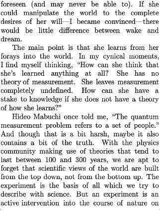
foreseen (and may never be able to). If she

could manipulate the world to the complete

desires of her will—I became convinced—there

would be little difference between wake and

dream.

The main point is that she learns from her

forays into the world. In my cynical moments,

Ifind myself thinking, “How can she think that

she’s learned anything at all? She has notheory ofmeasurement. She leaves measurement

completely undefined. How can she have astake to knowledge if she does not have a theory

of how she learns?”

Hideo Mabuchi once told me, “The quantum

measurement problem refers to a set of people.”

And though that isa bit harsh, maybe it also

contains a bit of the truth. With the physics

community making use of theories that tend to

last between 100 and 300 years, we are apt to

forget that scientific views of the world are built

from the top down, not from the bottom up.The

experiment is the basis of all which we try to

describe with science. But an experiment is anactive intervention into the course of nature on

the part of the experimenter; it is not

contemplation of nature from afar [44].We set

up this or that experiment to see how nature

reacts. It is the conjunction of myriads of such

interventions and their consequences that werecord into our data books. 18

We tell ourselves that we have learned

something new when we can distill from the

data a compact description of all that was seenand—even more tellingly—when we can dream

up further experiments to corroborate that

description. This is the minimal requirement of

science. If, how-ever, from such a description wecan further distill a model of a free-standing

“reality” independent of our interventions, then

so much the better.Ihave no bone topick with

reality. It is the most solid thing we can hope for

from a theory. Classical physics is the ultimate

example in that regard. It gives us a compact

description, but it can give much more if wewant it to.

The important thing to realize, however, is

that there is no logical necessity that such aworld-view always be obtainable. If the world is

such that we can never identify a reality—a

free-standing reality—independent of ourexperimental interventions, then we must be

prepared for that too. That is where quantum

theory in its most minimal and conceptually

simplest dispensation seems to stand [46]. It isatheory whose terms refer predominately to ourinterface with the world. It is a theory that

cannot go the extra step that classical physics

did without “writing songs Ican’t

18But Imust stress that Iam not so positivistic as to

think that physics should somehow be grounded on a

primitive notion of “sense impression” as the philosophers

of the Vienna Circle did. The interventions and their

consequences that an experimenter records, have no

option but to be thoroughly theory-laden. It is just

that, inasense, they are by necessity at least one theory

behind. No one got closer to the salient point than

Heisenberg (in a quote he attributed to Einstein many

years after the fact)[45]:

It is quite wrong to try founding a theory on

observable magnitudes alone. Inreality the very opposite

happens. It is the theory which decides what we

canobserve. You must appreciate that observation

is avery complicated process. The phenomenon

under observation produces certain events inour

measuring apparatus. As a result, further processes

take place inthe apparatus, which eventually and

by complicated paths produce sense impressions

and help us to fix theeffects inour consciousness.

Along this whole path—from the phenomenon to

its fixation inour consciousness—we must beable to

tell how nature functions, must know the natural

laws at least inpractical terms, before we canclaim

to have observed anything at all.Only theory, that

is,knowledge of natural laws, enables ustodeduce

the underlying phenomena from our sense

impressions. When we claim that we can observe

something

new, we ought really to be saying that, although

we are about toformulate new natural laws that do

not agree with the old ones, we nevertheless

assume that theexisting laws—covering the whole path

from the phenomenon to our

consciousness—function insuch a way that we can rely

upon them and

hence speak of “observation.”

13

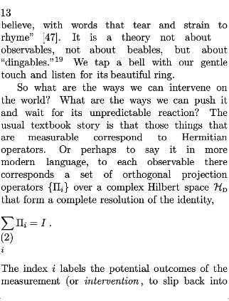
believe, with words that tear and strain to

rhyme” [47]. It is a theory not about

observables, not about beables, but about

“dingables.” 19 We tap a bell with our gentle

touch and listen for its beautiful ring.

So what are the ways we can intervene onthe world? What are the ways we can push it

and wait for its unpredictable reaction? The

usual textbook story is that those things that

are measurable correspond to Hermitian

operators. Or perhaps to say it in moremodern language, to each observable there

corresponds a set of orthogonal projection

operators Πi over a complex Hilbert space HD

that form acomplete resolution of the identity,

Xi

Πi =I.(2)

The index ilabels the potential outcomes of the

measurement (or intervention ,to slip back into

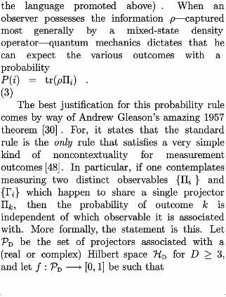
the language promoted above) .When anobserver possesses the information ρ—captured

most generally by a mixed-state density

operator—quantum mechanics dictates that he

can expect the various outcomes with aprobability

P(i) = tr(ρΠi ) .(3)

The best justification for this probability rule

comes by way of Andrew Gleason’s amazing 1957

theorem [30].For, it states that the standard

rule is the only rule that satisfies a very simple

kind of noncontextuality for measurement

outcomes [48].Inparticular, if one contemplates

measuring two distinct observables Πi and

Γi which happen to share a single projector

Πk,then the probability of outcome k is

independent of which observable it is associated

with. More formally, the statement is this. Let

PD be the set of projectors associated with a(real or complex) Hilbert space HD for D ≥ 3,

and let f:PD −→ [0,1] be such that

Xi

f(Πi )=1

(4)

whenever a set of projectors Πi forms anobservable. The theorem concludes that there

exists a density operator ρ such that

f(Π) = tr(ρΠ) .(5)

In fact, in a single blow, Gleason’s theorem

derives not only the probability rule, but also

the state-space structure for quantum mechanical

states (i.e., that it corresponds to the convex set

of density operators).

In itself this is no small feat, but the thing

that makes the theorem an “amazing” theorem

is the sheer difficulty required to prove it [49].Note that no restrictions have been placed uponthe function f beyond the ones mentioned above.

There is no assumption that it need be

differentiable, nor that it even need be continuous.

All of that, and linearity too, comes from the

structure of the observables—i.e., that they are

complete sets of orthogonal projectors onto alinear vector space.

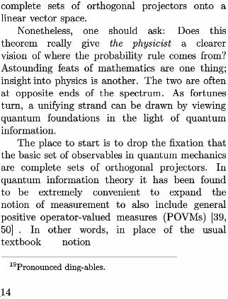
Nonetheless, one should ask: Does this

theorem really give the physicist a clearer

vision of where the probability rule comes from?

Astounding feats of mathematics are one thing;

insight into physics isanother. The two are often

at opposite ends of the spectrum. As fortunes

turn, a unifying strand can be drawn by viewing

quantum foundations in the light of quantum

information.

The place to start is to drop the fixation that

the basic set of observables inquantum mechanics

are complete sets of orthogonal projectors. In

quantum information theory it has been found

to be extremely convenient to expand the

notion of measurement to also include general

positive operator-valued measures (POVMs) [39,

50].In other words, in place of the usual

textbook notion

19Pronounced ding-ables.

14

of measurement, any set Ed of

positive-semidefinite operators on HD that forms

a resolution of the identity, i.e., that satisfies

hψ|Ed |ψi ≥ 0, for all |ψi ∈ HD

(6)

andXd

Ed =I,(7)

counts asameasurement. The outcomes of the

measurement are identified with the indices d,

and the probabilities of the outcomes arecomputed according toageneralized Born rule,

P(d) =tr(ρEd ).(8)

The set Ed is called a POVM, and the

operators Ed are called POVM elements. (In

the non-standard language promoted earlier, the

set Ed signifies an intervention into nature,

while the individual Ed represent the potential

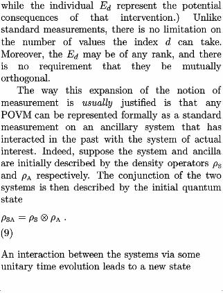
consequences of that intervention.) Unlikenature, while the

standard measure-ments, there is no limitation onthe number of values the index d can take.

Moreover, the Ed may be of any rank, and there

is no requirement that they be mutually

orthogonal.

The way this expansion of the notion of

measurement is usually justified is that anyPOVM can be represented formally as a standard

measurement on an ancillary system that has

interacted in the past with the system of actual

interest. Indeed, suppose the system and ancilla

are initially described by the density operators ρS

and ρA respectively. The conjunction of the two

systems is then described by the initial quantum

state

ρSA =ρS ⊗ ρA .(9)

Aninteraction between the systems via someunitary time evolution leads toanew state

ρSA −→ UρSA U† .

(10)

Now, imagine a standard measurement on the

ancilla. It is described on the total Hilbert spacevia a set of orthogonal projection operators I⊗Πd . An outcome d will be found, by the

standard Born rule,with probability

P(d) =tr‡U(ρS

⊗ ρA )U†(I ⊗ Πd )

· .(11)

The number of outcomes in this seemingly

indirect notion of measurement is limited only

by the dimensionality of the ancilla’s Hilbert

space—in principle, there can be arbitrarily

many.As advertised, it turns out that the

probability formula above can be expressed in

terms of operators on the system’s Hilbert spacealone: This is the origin of the POVM. If we let

|sαiand |acibe an orthonormal basis for the

system and ancilla respectively, then |sα i|aciwe let|sα iand

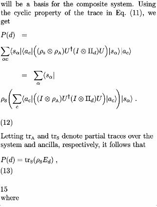
will be a basis for the composite system. Using

the cyclic property of the trace in Eq. (11), weget

P(d) =Xαc

hsα |hac |

‡(ρs

⊗ ρA )U†(I

⊗ Πd )U

·|sα

i|ac i

=Xα

hsα

ρS

ˆXc

hac |

‡(I

⊗ ρA )U†(I ⊗ Πd )U

·|ac

i

!|sα

i.(12)

Letting trA and trS denote partial traces over the

system and ancilla, respectively, it follows that

P(d) = trS (ρS Ed),(13)

15

where

Ed = trA

‡(I

⊗ ρA )U†(I

⊗ Πd )U

·

(14)

‡(I

is an operator acting on the Hilbert space of the

·

original system. This proves half of what is

needed, but it is also straightforward to go in the

reverse direction—i.e., to show that for anyPOVM Ed , one can pick an ancilla and find

operators ρA,U, and Πd such that Eq. (14) isanytrue.

Putting this all together, there is a sense in

which standard measurements capture

everything that can be said about quantum

measurement theory [50].As became clear above,

a way to think about this is that by learning

something about the ancillary system through astandard measure-ment, one in turn learns

something about the system of real interest.

Indirect though it may seem, this can be apowerful technique, sometimes revealing

information that could not have been re-vealed

otherwise [51].A very simple example is where asender has only a single qubit available for the

sending one of three potential messages. She

therefore has a need to encode the message inoneof three preparations of the system, even though

the system is a two-state system. To recover asmuch information as possible, the receiver might

(just intuitively) like to perform a measurement

with three distinct outcomes. If, however, he

were limited to a standard quantum

measurement, he would only be able toobtain two

outcomes. This—perhaps surprisingly—generally

degrades his opportunities for recovery.What Iwould like to bring up is whether

this standard way of justifying the POVM is

the most productive point of view one can take.

Might any of the mysteries of quantum

mechanics be alleviated by taking the POVM asa basic notion of measurement? Does the

POVM’s utility portend a larger role for it inthe

foundations of quantum mechanics?

Standard Generalized

Measurements Measurements

Πi Ed

hψ|Πi |ψi ≥ 0,∀|ψi hψ|Ed |ψi ≥ 0,∀|ψi

Pi

Πi =I Pd

Ed =I

P(i)=tr(ρΠi ) P(d) = tr(ρEd )

Πi Πj =δij Πi ———

Itry to make this point dramatic in mylectures by exhibiting a transparency of the

table above. On the left-hand side there is alist of various properties for the standard

notion of a quantum measurement. On the

right-hand side, there is an almost identical list

of properties for the POVMs. The only

difference between the two columns is that the

right-hand one is missing the orthonormality

condition required of a standard measurement .The question Iask the audience is this: Does the

addition of that one extra assumption really

make the process of measurement any less

mysterious? Indeed, Iimagine myself teaching

quantum mechanics for the first time and taking

a vote with the best audience of all, the

students. “Which set of postulates for quantum

measurement would you prefer?” Iam quite surethey would respond withablank stare. But that

16

is the point! It would make no difference to

them, and it should make no difference to us.The only issue worth debating iswhich notion of

measurement will allow us to see more deeply

into quantum mechanics.

Therefore let us pose the question that

Gleason did, but with POVMs. Inother words,

let us suppose that the sum total of ways anexperimenter can intervene on a quantum system

corresponds to the full set of POVMs on its Hilbert

space HD.It is the task of the theory to give him

probabilities for the various consequences of his

interventions. Concerning those probabilities, let

us (in analogy to Gleason) assume only that

whatever the probability for agiven consequenceEc is, it does not depend upon whether Ec is

associated with the POVM Ed or, instead, anyisother one Ed.This means we can assume thereassociated with t

exists a function

f:ED −→ [0,1] ,(15)

where

ED =nE

:0≤ hψ|E|ψi ≤ 1,∀ |ψi ∈ HD

o ,(16)

such that whenever Ed forms a POVM,

f(Ed )=1.(17)

(Ingeneral, we will callany function satisfying

f(E) ≥ 0 andXd

f(Ed )=constant

(18)

a frame function, inanalogy to Gleason’s

nonnegative frame functions. The set ED isoften

called the set of effects over HD .)

Itwillcome asnosurprise, of course, that aGleason-like theorem must hold for the function

inEq.(15). Namely, itcan be shown that there

must exist adensity operator ρ for which

f(E)=tr(ρE) .(19)

This was recently shown by Paul Busch [28] and,

independently, by Joseph Renes and collabora-

tors [29].What is surprising however is the utter

simplicity of the proof. Let us exhibit the whole

thing right here and now.

First, consider the case where HD and the

operators on it are defined only over the field ofFirst, con sider thecase whe reH D

(complex) rational numbers. It is no problem to

see that f is “linear” with respect to positive

combinations of operators that never go outside ED .positiv ecom bin ation

For consider a three-element POVM E1,E2,E3.of operators that nevergo out side ED

By assumption f(E1)+ f(E2 )+ f(E3 )=1.However,PO VM E1 . By ass

we can also group the first two elements in thismption f(E1

POVM to obtain a new POVM, and must therefore

have f(E1 + E2 )+f(E3 )= 1. In other words, the

function f must be additive with respect to afine-graining operation:

f(E1 + E2 ) = f(E1) + f(E2 ) .(20)

Similarly for any two integers mand n,

f(E) =mf

?1

mE

¶

=nf

?1

nE

¶

(21)

Supposen

m≤ 1.Then if we write E=nG, this

statement becomes:

f

‡n

mG

·= n

mf(G) .

(22)

17

Thus we immediately have a kind of limited linearity

on ED .Thus we imme diately have a kind of limite dlinea rity

One might imagine using this property to cap offon ED

the theorem in the following way. Clearly the full2-dimensional

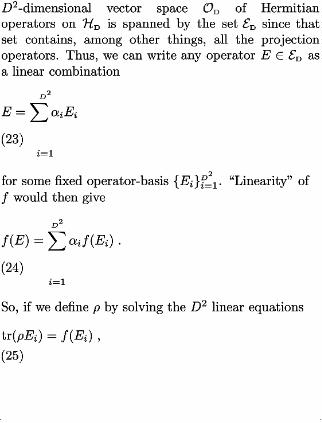
D vector space OD of Hermitian

operators on HD is spanned by the set ED since thatv ector sp ace O D of Herm itia noperator

set contains, among other things, all the projectiononHD ED

operators. Thus, we can write any operator E∈ ED asa linear combination

D2

Xi=1

E=Xi=1

αi Ei

(23)

Xi=1

for some fixed operator-basis Ei D2

i=1.“Linearity” of

fwould then give

D2

Xi=1

f(E) =Xi=1

αi f(Ei).(24)

Xi=1

So, ifwe define ρ by solving the D2 linear equations

tr(ρEi )=f(Ei ),(25)

we would have

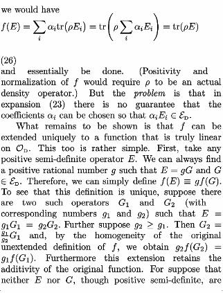
f(E) =Xi

αi tr¡ρEi ¢

=tr

ˆρ

Xi

αi Ei

!

=tr(ρE)

(26)

and essentially be done. (Positivity and

normalization of f would require ρ to be an actual

density operator.) But the problem is that in

expansion (23) there is no guarantee that the

coefficients αi canbechosen so that αi Ei ∈ ED . ∈ E D

What remains to be shown is that f can be

extended uniquely to a function that is truly linear

on OD.This too is rather simple. First, take anylinearon OD

positive semi-definite operator E.We can always find

a positive rational number g such that E=gG and Gcan alw ays finda pos itive rat

∈ ED.Therefore, we can simply define f(E) ≡ gf(G).onalnu mbe rg s uch that E = gG an dG ∈ ED

To see that this definition is unique, suppose theresimply de fine f(E )≡ gf(G)

are two such operators G1 and G2 (withTo see that this defini tio nis uniq ue,su ppos et he

corresponding numbers g1 and g2)such that E=are tw osuch

g1G1 = g2 G2 . Further suppose g2 ≥ g1.Then G2 =g1

g2G1 and, by the homogeneity of the original

unextended definition of f, we obtain g2 f(G2 ) =g1f(G1). Furthermore this extension retains the

additivity of the original function. For suppose that

neither Enor G, though positive semi-definite, are

necessarily in ED .We can find a positive rationalnec essanumber c ≥ 1such that 1c (E+ G),

1c E,and 1cG arerily in ED .We c an find a pos itiv erat ional nu

all in ED.Then, by the rules we have alreadymber c ≥ 1such that

obtained,

f(E+G)=cf

?1c

(E+G)

¶

=cf

?1c

E

¶

+cf

?1c

G

¶

=f(E)+ f(G).

(27)

Let us now further extend f’s domain to the full

space OD.This can be done by noting that anyoperator Hcan be written as the difference H=E−

G of two positive semi-definite operators. Therefore

define f(H) ≡ f(E) − f(G), from which it also

follows that f(−G) = −f(G). To see that this

definition is unique suppose there are four operators

E1,E2,G1,and G2,such that H=E1 − G1 =E2 −

G2.It follows that E1 +G2 =E2 +G1.Applying f

(as extended in the previous paragraph) to this

equation, we obtain f(E1)+f(G2 )= f(E2 )+f(G1) sothat f(E1) − f(G1)= f(E2 )− f(G2 ).Finally, with

this new extension, full linearity can be checked

immediately. This completes the proof as far as the

(complex) rational number field is concerned: Because

f extends uniquely to a linear functional on OD,wecan indeed go through the steps of Eqs. (23) through

(26) without worry.

There are two things that are significant

about this much of the proof. First, incontrast

to Gleason’s original theorem, there is nothing

to bar the same logic from working when D=2. This is quite nice because much of the

community has gotten into the habit of

thinking that

18

there isnothing particularly “quantum

mechanical” about asingle qubit.[52] Indeed,

because orthogonal projectors on H2 canbe

mapped onto antipodes of the Bloch sphere, it isorthogonal projectors on H2

known that the measurement-outcome statistics

forany standard measurement can be

mocked-up through a noncontextual

hidden-variable theory. What this result shows

isthat that simply isnot the case when oneconsiders the fullset of POVMs asone’s

potential measurements. 20

The other important thing is that the theorem

works for Hilbert spaces over the rational number

field: one does not need to invoke the fullpower of

the continuum. This contrasts with the surprising

result of Meyer[54] that the standard Gleason

theorem fails insuch asetting. The present

theorem hints at akind of resiliency to the

structure of quantum mechanics that falls

through the mesh of the standard Gleason result:

The probability rule for POVMs does not

actually depend somuch upon the detailed

workings of the number field.

The final step of the proof, indeed, is to

show that nothing goes awry when wego the

extra step of reinstating the continuum.

Inother words, we need to show that the

function f (now defined on the set ED of

complex operators) isacontinuous

function. This comes about inasimple wayED

from

f’s additivity. Suppose for two positive

semi-definite operators Eand G that E≤ G

(i.e., G−E is positive semi-definite). Then

trivially there exists a positive semi-definite

operator Hsuch that E+H=G and

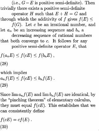
through which the additivity of fgives f(E) ≤

f(G).Let cbeanirrational number, and

let an be an increasing sequence and bn adecreasing sequence of rational numbers

that both converge toc.It follows foranypositive semi-definite operator E,that

f(an E)≤ f(cE) ≤ f(bn E),(28)

which implies

an f(E) ≤ f(cE) ≤ bn f(E) .(29)

Since liman f(E) and limbn f(E)are identical, by

the “pinching theorem” of elementary calculus,

they must equal f(cE). This establishes that wecan consistently define

f(cE) =cf(E) .(30)

Reworking the extensions of f in the last

inset (but with this enlarged notion of homo-

geneity), one completes the proof in astraightforward manner.

Of course we are not getting something from

nothing. The reason the present derivation is soeasy in contrast to the standard proof is that

mathematically the assumption of POVMs as the

basic notion of measurement is significantly

stronger than the usual assumption. Physically,

though, Iwould say it is just the opposite. Why

add extra restrictions to the notion of

measurement when they only make the route

from basic assumption to practical usage morecircuitous than need be?

Still, no assumption should be left unanalyzed

if it stands a chance of bearing fruit. Indeed, onecan ask what is so very compelling about the

noncontextuality property (of probability

assignments) that both Gleason’s original

theorem and the present version make use of.

Given the picture of measurement as a kind of

invasive intervention into the world, one might

expect the very opposite. One is left wondering

why measurement probabilities do not depend

upon the whole context of the measurement

interaction. Why is P(d) not of the form f(d,mea surem en)? Is there any good reason for this kind of

assumption?

20In fact, one need not consider the full set of POVMs

in order to derive a noncolorability result along the lines

of Kochen and Specker for a single qubit. Considering

only 3-outcome POVMs of the so-called “trine” or

“Mercedes-Benz” type already does the trick.[53]

19

4.1 Noncontextuality

In point of fact, there is: For, one can arguethat the noncontextuality of probability

assignments for measurement outcomes is morebasic than even the particular structure of

measurements (i.e., that they be POVMs).

Noncontextuality bears more onhow we identify

what we are measuring than anything todo with

ameasurement’s invasiveness upon nature.

Here is a way to see that. [55] Forget about

quantum mechanics for the moment and consider

a more general world—one that, skipping the

details of quantum mechanics, still retains the

notions of systems, machines, actions, and

consequences, and, most essentially, retains the

notion of a scientific agent performing those

actions and taking note of those consequences.Take a system S and imagine acting on it

with one of two machines, Mand N—things that

we might colloquially call “measurement devices”

if we had the aid of a theory like quantum

mechanics. For the case of machine M, let us label

the possible consequences of that action m1,m2,....(Or if you want to think of them inthe mold

of quantum mechanics, call them “measurement

outcomes.”) For the case of machine N, let uslabel them n1,n2 ,....

If one takes a Bayesian point of view about

probability, then nothing can stop the agents in

this world from using all the information available

to them to ascribe probabilities to the

consequences of those two potential actions. Thus,

for an agent who cares to take note, there are two

probability distributions, pM (mk ) and pN (nk ),

lying around. These probability distributions

stand for his subjective judgments about what

will obtain if he acts with either of the two

machines.

This is well and good, but it is hardly aphysical theory. We need more. Let us supposethe labels mk and nk are, at the very least, to

be identified with elements in some master set

F— that is, that there is some kind of

connective glue for comparing the operation ofmas terset F—

one machine to another. This set may even be aset with further structure, like a vector space orsomething, but that is beside the point. What is

of first concern is under what conditions will anagent identify two particular labels mi and nj

with the same element F in the master set

—disparate in appearance, construction, and

history though the two machines Mand Nmaybe. Perhaps one machine was manufactured by

Lucent Technologies while the other wasmanufactured by IBMCorporation.

There is really only one tool available for

the purpose, namely the probability

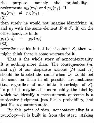
assignments pM (mi)and pN (nj ).If

pM (mi ) 6= pN (nj ) ,(31)

then surely he would not imagine identifying mi

and nj with the same element F∈ F.If,on the

other hand, he finds

pM (mi ) = pN (nj )

(32)

regardless of his initial beliefs about S, then wemight think there issome warrant for it.

That is the whole story of noncontextuality.

It is nothing more than: The consequences (mi

and nj )of our disparate actions (M and N)

should be labeled the same when we would bet

the same on them inall possible circumstances

(i.e., regardless of our initial knowledge of S).

To put this maybe a bit more baldly, the label by

which we identify a measurement outcome is asubjective judgment just like a probability, and

just like aquantum state.

By this point of view, noncontextuality is atautology—it is built in from the start. Asking

why we have it is a waste of time. Where wedo have a freedom is inasking why we make

one particular choice of a master set overanother. Asking that may tell us something

about physics. Why should the mi ’s be drawn

from a set of effects ED?Not allchoices of the

master set are equally interesting once we have

settled on noncontextuality for the probability

assignments. 21 But quantum mechanics, of course,isparticularly interesting!

21See Ref. [56], pp. 86–88, and Ref. [57] for some

examples inthat regard.

20

4.2 LeBureau International des Poids

et Mesures `aParis

There is still one further, particularly

important, advantage to thinking of POVMs asthe basic notion of measurement in quantum

mechanics. For with an appropriately chosen

single POVM one can stop thinking of the

quantum state as a linear operator altogether,

and instead start thinking of it as aprobabilistic

judgment with respect to the (potential)

outcomes of a standard quantum measurement.

That is, a measurement device right next to the

standard kilogram and the standard meter in acarefully guarded vault,deep within the bowels

of the International Bureau of Weights and

Measures. 22 Here iswhat Imean by this.

Our problem hinges on finding ameasurement for which the probabilities of

outcomes com-pletely specify a unique density

operator. Such measurements are called

informationally complete and have been studied

for some time [60, 61, 62]. Here however, the

picture is most pleasing if we consider a slightly

refined version of the notion—that of the minimal

informationally complete mea-surement [32].The

space of Hermitian operators on HD is itself asurement[32]. Th

linear vector space of dimension D2.The quantityspace of Herm itian opera tors on HD

tr(A †B) serves as an inner product on that space.Hence, if we can find a POVM E = Ed

consisting of D2 linearly independent operators,

the probabilities P(d) =tr(ρEd )—now thought of

as projections inthe directions of the vectors Ed

—will completely specify the operator ρ. Any two

distinct density operators ρ and σ must give rise

to distinct outcome statistics for this

measurement .The minimal number of

outcomes a POVM can have and still be

informationally complete isD2.

Do minimal informationally complete

POVMs exist? The answer is yes. Here is asimple way to produce one, though there aremany other ways. Start with a complete

orthonormal basis |ej ion HD.It is easy to checkere aremany othe rw ays.St art with a com plete

that the following D2 rank-1 projectors Πd formona linearly independent set.

1.For d=1,...,D, let

Πd = |ej ihej |,

(33)

where j,too, runs over the values 1,...,D.

2.For d=D+1,...,12D(D+1),let

Πd = 12(|ej i+ |ek i)(hej |+ hek |),

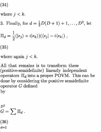
(34)

where j<k.

3.Finally, for d= 12D(D+1)+1,...,D 2,let

Πd = 12(|ej i+ i|ek i)(hej |− ihek |),

(35)

where again j<k.

Allthat remains isto transform these

(positive-semidefinite) linearly independent

operators Πd into aproper POVM. This can be

done by considering the positive semidefinite

operator Gdefined

by

D2

X

G=X

Πd .(36)X

d=1

22This idea has itsroots inL.Hardy’s two important

papers Refs. [58] and [59].

21

It is straightforward to show that hψ|G|ψi > 0

for all |ψi 6= 0, thus establishing that G is

positive definite (i.e., Hermitian with positive

eigenvalues) and hence invertible. Applying the

(invertible) linear transformation X →

G−1/2XG −1/2 to Eq.

(36),we find avalid decomposition of the identity,

D2

X

I=X

G−1/2Πd

G−1/2 .

(37)

X

d=1

The operators

Ed = G−1/2Πd

G−1/2

(38)

satisfy the conditions of a POVM, Eqs. (6) and

(7), and moreover, they retain the rank and

linear independence of the original Πd.Thus we

have what we need.

With the existence of minimal

informationally complete POVMs assured, wecan think about the vault in Paris. Let ussuppose from here out that it contains a machine

that enacts a minimal informationally complete

POVM Eh whenever it is used. We reserve the

index h to denote the out-comes of this standard

quantum measurement ,for they will replace the

notion of the “hypothesis” in classical statistical

theory. Let us develop this from a Bayesian

point of view.

Whenever one has a quantum system in

mind, it is legitimate for him touse allhe knows

and believes of it to ascribe a probability

function P(h) to the (potential) outcomes of

this standard measurement. In fact, that isallaquantum state is from this point of view: It is

a subjective judgment about which consequencewill obtain as a result of an interaction between

one ’s system and that machine. Whenever oneperforms a measurement Ed on theand that macsystem—one different from the standard

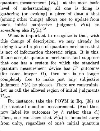
quantum measurement Eh —at the most basic

level of understanding, all one is doing is

gathering (or evoking) a piece of data d that

(among other things) allows one to update from

one’s initial subjective judgment P(h) to

something else Pd (h).23

What is important to recognize is that, with

this change of description, we may already be

edging toward apiece of quantum mechanics that

is not of information theoretic origin. It is this.

If one accepts quantum mechanics and supposesthat one has a system for which the standard

quantum measurement device has D2 outcomes

(for some integer D), then one is no longer

completely free to make just any subjective

judgment P(h) he pleases. There are constraints.

Let us call the allowed region of initial judgments

PSQM .For instance, take the POVM inEq. (38) as

the standard quantum measurement. (And thus,

now label its outcomes by h rather than d.)

Then, one can show that P(h) is bounded awayfrom unity, regardless of one’s initial quantum

state for the system. Inparticular,

P(h) ≤ maxρ

tr(ρEh )

≤ maxΠ

tr(ΠEh )

≤ λmax (Eh )

= λmax (G−1/2Πh

G−1/2) =λmax (Πh G

−1Πh)

≤ λmax (G−1) ,

(39)

where the second line above refers toamaximization over allone dimensional projectors

and λmax (·) denotes the largest eigenvalue of its

argument. On the other hand, one can calculate

the eigenvalues of G−1 explicitly.[63] Through

this,one obtains

P(h) ≤

•D

−12

?1

+cot3π

4D

¶‚−1

<1.(40)

23Wewillcome back todescribing the precise formof

this update and itssimilarity toBayes’ rule inSection 6.

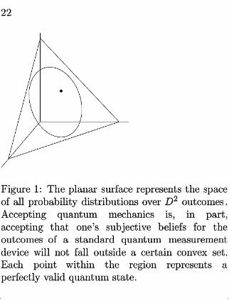
22

Figure 1:The planar surface represents the spaceof all probability distributions over D2 outcomes .Accepting quantum mechanics is, in part,

accepting that one’s subjective beliefs for the

outcomes of a standard quantum measurement

device will not fall outside a certain convex set.

Each point within the region represents aperfectly valid quantum state.

For large D, this bound asymptotes to roughly

(0.79D) −1.

More generically, for any minimal

informationally complete POVM Eh ,P(h) must

be bounded away from unity for all its possible

outcomes. Thus even at this stage, there is

something driving a wedge between quantum

mechanics and simple Bayesian probability

theory. When one accepts quantum mechanics,

one voluntarily accepts a restriction on one’s

subjective judgments for the consequences of astandard quantum measurement intervention:

For all consequences h, there are no conditions

whatsoever convincing enough to compel one to

a probability ascription P(h) = 1. That is, onegives up on the hope of certainty. This, indeed,

one might pinpoint as an assumption about the

physical world that goes beyond pure probability

theory. 24

But what is that assumption in physical

terms? What is our best description of the

wedge?

Some think they already know the answer,

5 Wither Entanglement?25

and it is quantum entanglement.

When two systems, of which we know the states by their re-

spective representatives, enter into temporary physical inter-

action due toknown forces between them, and when after a

time of mutual influence the systems separate again, then they

canno longer bedescribed inthe same way asbefore, viz.by

endowing each of them witharepresentative of its own. I

would not callthat one but rather the characteristic trait of

quantum mechanics, the one that enforces its entire departure

from classical lines of thought. By the interaction the two rep-

resentatives (orψ-functions) have become entangled.

— Erwin Schr¨ odinger, 1935

24It is at this point that the present account of

quantum mechanics differs most crucially from Refs. [58]

and [59]. Hardy sees quantum mechanics as a

generalization and extension of classical probability

theory, whereas quantum mechanics is depicted here as a

restriction to probability theory. It is a restriction that

takes into account how we ought to think and gamble in

light of acertain physical fact—a fact we are working like

crazy to identify.25

This isnot aspelling mistake.

23

Quantum entanglement has certainly

captured the attention of our community. By

most ac-counts it is the main ingredient in

quantum information theory and quantum

computing [64],and it is the main mystery of the

quantum foundations [65].But what is it?Where

does it come from?

The predominant purpose it has served in

this paper has been as a kind of background.

For it, more than any other ingredient in

quantum mechanics, has clinched the issue of

“information about what?” inthe author’s mind:

That information cannot be about a preexisting

reality (a hidden variable) unless we are willing

to renege on our reason for rejecting the

quantum state’s objective reality in the first

place. What Iam alluding to here is the

conjunction of the Einstein argument reported in

Section 3 and the phenomena of the Bell

inequality violations by quantum mechanics.

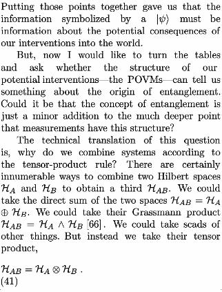
Putting those points together gave us that themeinformation symbolized by a |ψi must be

information about the potential consequences ofhat the information symbolized

our interventions into the world.

But, nowIwould like to turn the tables

and ask whether the structure of ourpotential interventions—the POVMs—can tellussomething about the origin of entanglement.

Could it be that the concept of entanglement is

just a minor addition to the much deeper point

that mea-surements have this structure?

The technical translation of this question

is,why do we combine systems according to

the tensor-product rule? There are certainly

innumerable ways to combine two Hilbert spacesHA and HB to obtain a third HAB.We could

take the direct sum of the two spaces HAB = HA

⊕ HB.We could take their Grassmann product

HAB = HA ∧ HB [66].We could take scads ofcoul dtake t hei rGra ssma nnproother things. But instead we take their tensor

product,

HAB =HA ⊗ HB .(41)

Why?

Could it arise from the selfsame

considerations as of the previous

section—namely, from a noncontextuality

property for measurement-outcome

probabilities? The answer is yes, and the

theorem Iam about demonstrate owes much in

inspiration toRef. [67]. 26

Here is the scenario. Suppose we have two

quantum systems, and we can make ameasurement on each. On the first, we canmeasure any POVM on the DA -dimensional

Hilbert space HA;on the second, we canmeasure any POVM on the DB -dimensional

Hilbert space HB . (This, one might think, is

the very essence of having two systems rather

than one—i.e., that we can probe them

independently.) Moreover, suppose we maycondition the second measurement on the nature

and the outcome of the first, and vice versa.That is to say—walking from A to B—we could

first measure Ei on A, and then, depending onthe outcome i, measure F i

j on B.meas ur eEion A,and then

Similarly—walking from B to A—we could first

measure Fj on B, and then, depending on the

outcome j,measure Ej

ion A.So that we have

valid POVMs, we must have

Xi

Ei =I andXj

Fi

j=I ∀i ,

(42)Xi X

andXi

Ej

i=I ∀j and

Xj

Fj =I,(43) ∀j

X

for these sets of operators. Let us denote by Sij

anordered pair of operators, either of the form

(Ei ,F i

j)orof the form (E

j

i,Fj ),as appearing

above. Let us call a set of such operators Sij

a locally-measurable POVM tree.

26After posting Ref. [1],Howard Barnum andAlex Wilce

brought tomy attention that there isasignificant amount

of literature inthe quantum logic community devoted to

similar ways of motivating the tensor-product rule.See

for example Ref. [68] and themany citations therein.

24

Suppose now that—just as with the

POVM-version of Gleason’s theorem in Section 4

—the joint probability P(i,j)for the outcomes of

such a measurement should not depend uponwhich tree Sij is embedded in:This is essentially

the same assumption we made there, but nowapplied to local measurements on the separate

systems. In other words, let us suppose there

exists a function

f:EDA ×EDB −→ [0,1]

(44)

such thatXij

f(Sij ) = 1

(45)Xij

whenever the Sij satisfy either Eq. (42) or Eq.

(43).

Note in particular that Eq. (44) makes nouse of the tensor product: The domain of f is

the Cartesian product of the two sets EDA and EDB.

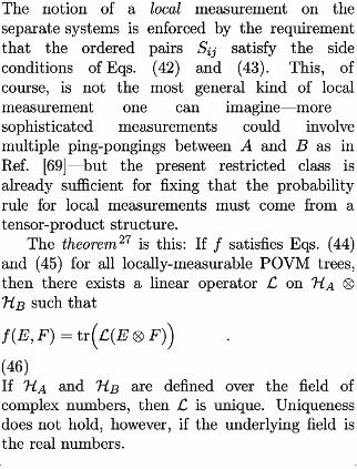
The notion of a local measurement on the

separate systems is enforced by the requirement

that the ordered pairs Sij satisfy the side

conditions of Eqs. (42) and (43). This, of

course, is not the most general kind of local

measurement one can imagine—more

sophisticated measurements could involve

multiple ping-pongings between A and B as in

Ref. [69]—but the present restricted class is

already sufficient for fixing that the probability

rule for local measurements must come from atensor-product structure.

The theorem 27 is this: If f satisfies Eqs. (44)

and (45) for all locally-measurable POVM trees,

then there exists a linear operator L on HA ⊗

HB such that

f(E,F) =tr‡L(E

⊗ F)

· .(46)

If HA and HB are defined over the field of

complex numbers, then L is unique. Uniqueness

does not hold, however, if the underlying field iscomplex numbers

the realnumbers.

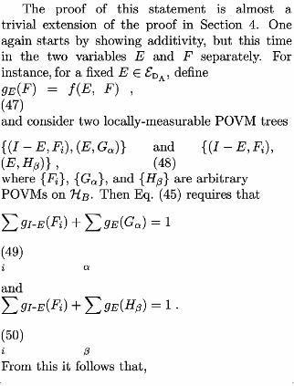
The proof of this statement is almost atrivial extension of the proof inSection 4.One

again starts by showing additivity, but this time

in the two variables Eand F separately. For

instance, for a fixed E∈ EDA ,define

gE (F) = f(E, F) ,(47)

and consider two locally-measurable POVM trees

(I− E,Fi ),(E,Gα ) and (I− E,Fi ),

(E,Hβ ), (48)

where Fi ,Gα ,and Hβ are arbitrary

POVMs on HB.Then Eq.(45) requires that

Xi

gI-E (Fi)+Xα

gE (Gα )=1

(49)X

andXi

gI-E (Fi)+Xβ

gE (Hβ )=1.(50)

X

From this it follows that,

Xα

gE (Gα )=Xβ

gE (Hβ )=const.

(51)

Xα X

That istosay, gE (F) isa frame function inthe

sense of Section 4.Consequently, we know that

we can use the same methods as there touniquely

extend gE (F) toa linear functional on the

complete set of Hermitian operators on HB

Similarly, for fixed F∈ EDB,we can define

hF (E)=f(E,F) ,(52)

27InRef. [1],a significantly stronger claim is made:

Namely, that Lis in fact a density operator. This was aRef. [1],a significantly stronger

flat-out mistake. See further discussion below.

25

and prove that this function too can be extended

uniquely to a linear functional on the Hermitian

operators on HA .The linear extensions of gE (F) and hF (E)

can be put together ina simple way to give afull bilinear extension to the function f(E,F).

Namely, for any two Hermitian operators A and

B on HA and HB,respectively, let A = α1 E1 −

α2 E2 and B = β1 F1 − β2 F2 be decompositions

such that α1 ,α2 ,β1 ,β2 ≥ 0,E1,E2 ∈ EDA ,and F1,F2 ∈ EDB.Then define

f(A, B) ≡ α1 gE1 (B) − α2 gE2 (B) .(53)

To see that this definition is unique, take anyother decomposition

A = ˜α1 E1 − ˜α2 E2 .(54)

Then we have

f(A,B) = ˜α1 gE1

(B) − ˜α2 gE2

(B)

= ˜α1 f(E1,B) − ˜α2 f(E2 ,B)

= β1

‡˜

α1 f(E1,F1)− ˜α2 f(E2 ,F1)

·

− β2

‡˜

α1 f(E1,F2 )− ˜α2 f(E2 ,F2 )

·‡˜

= β1 hF1(A) − β2 hF2 (A)

= β1

‡α1

f(E1,F1)− α2 f(E2 ,F1)

·

− β2

‡α1

f(E1,F2 )− α2 f(E2 ,F2 )

·‡α1

= α1 f(E1,B) − α2 f(E2 ,B)

= α1 gE1 (B) − α2 gE2 (B) ,(55)

which isas desired.

With bilinearity for the function f

established, we have essentially the fullstory[66,

70].For, let Ei ,i=1,...,D 2

A,be a complete

basis for the Hermitian operators on HA and

let Fj , j=1,...,D 2

B,be a complete basis for

the Hermitian operators on HB . IfE=Pi

αi Ei and F= Pj

βj Fj,then

f(E,F) =Xij

αi βj f(Ei ,Fj ).(56)

Define L to be a linear operator on HA ⊗ HB

satisfying the (DA DB )2 linear equations

tr‡L(Ei

⊗ Fj )

·=f(Ei ,Fj ).

(57)

Such anoperator always exists. Consequently we

have,

f(E,F) =Xij

αi βj tr‡L(Ei

⊗ Fj )

·

= tr‡L(E

⊗ F)

· .(58)

For complex Hilbert spaces HA and HB ,the

uniqueness of L follows because the set Ei ⊗Fj

forms a complete basis for the Hermitian

operators on HA ⊗ HB .[71] For realHilbert

spaces, however, the analog of the Hermitian

operators are the symmetric operators. The

dimensionality of the space of symmetric

operators on a real Hilbert space HD is12D(D+

1),rather than the D2 it is for the complex case.This means that inthe steps above only

14DA DB (DA +1)(DB +1)

(59)

26

equations willappear inEq.(57), whereas

12DA DB (DA DB +1)

(60)

are needed to uniquely specify an L. For

instance take DA = DB = 2. Then Eq. (59)

gives nine equations, while Eq.(60) requires ten.

This establishes the theorem. It would be

nice if we could go further and establish the

full probability rule for local quantum

measurements—i.e., that L must be a density

operator. Unfor-tunately, our assumptions are not

strong enough for that. Here is acounterexample .[72] Consider a linear operator

that is proportional to the swap operator on the

two Hilbert spaces:

LS (E⊗ F)= 1

D2F⊗ E.

(61)

This clearly satisfies the conditions of our

theorem, but it is not equivalent to a density

operator.

Of course, one could recover positivity for L

by requiring that it give positive probabilities

even for nonlocal measurements (i.e., resolutions

of the identity operator on HA ⊗ HB ).But inventhe purely local setting contemplated here, that

would be a cheap way out. For, one should ask in

good conscience what ought to be the rule for

defining the full class of measurements (including

nonlocal measurements) :Why should it

correspond to an arbitrary resolution of the

identity on the tensor product? There is nothing

that makes it obviously so, unless one has

already accepted standard quantum mechanics.

Alternatively, it must be possible to give apurely local condition that will restrict L to be

a density operator. This is because L, asnoted above, is uniquely determined by theLto be

function f(E,F);we never need to look further

than the probabilities of local measurementsthe functi onoutcomes in specifying L. Ferreting out such acondition supplies an avenue for future research.

All of this does not, however, take awayfrom the fact that whatever L is, it must be alinear operator on the tensor product of HA and

HB.Therefore, let us close by emphasizing the

striking feature of this way of deriving the

tensor-product rule for combining separate

quantum systems: It is built on the very concept

of local measurement. There is nothing “spooky”

or “nonlocal” about it; there is nothing in it

resembling “passion at a distance” [73].Indeed,

one did not even have to consider probability

assignments for the outcomes of measurements

of the “nonlocality without entanglement” variety

[69] to uniquely fix the probability rule. That

is—to give an example on H3 ⊗ H3 —one need

not consider standard measurements like Ed =|ψd ihψd |,d=1,...,9, where

|ψ1i= |1i|1i

|ψ2i= |0i|0 +1i |ψ6i= |1+2i|0i

|ψ3i= |0i|0 − 1i |ψ7i= |1−

2i|0i (62) |ψ4i= |2i|1+ 2i

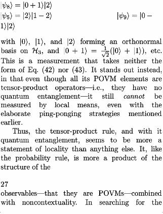
|ψ8 i= |0 +1i|2i

|ψ5i= |2i|1− 2i |ψ9i= |0 −

1i|2i

with |0i, |1i, and |2i forming an orthonormal

basis on H3,and |0 + 1i = 1√2 (|0i + |1i), etc.

This is a measurement that takes neither the

form of Eq. (42) nor (43). It stands out instead,

inthat even though all its POVM elements aretensor-product operators—i.e., they have noquantum entanglement—it still cannot be

measured by local means, even with the

elaborate ping-ponging strategies mentioned

earlier.

Thus, the tensor-product rule, and with it

quantum entanglement, seems to be more astatement of locality than anything else. It, like

the probability rule, is more a product of the

structure of the

27

observables—that they are POVMs—combined

with noncontextuality. In searching for the

secret ingredient to drive a wedge between

general Bayesian probability theory and

quantum mechanics, it seems that the direction

not to look is toward quantum entanglement.

Perhaps the trick instead is todig deeper into the

Bayesian toolbox.

6 Whither Bayes’ Rule?28

And so youseeIhave come todoubt AllthatIonce held

as trueIstand alone without beliefs The only truthIknow

isyou.

— Paul Simon,

timeless

Quantum states are states of information,

knowledge, belief, pragmatic gambling

commitments, not states of nature. That

statement is the cornerstone of this paper. Thus,

in searching to make sense of the remainder of

quantum mechanics, one strategy ought to be to

seek guidance [74] from the most developed

avenue of “rational-decision theory” to date

—Bayesian probability theory [75, 76, 77] .

Indeed, the very aim of Bayesian theory is to

develop reliable methods of reasoning and

making decisions in the light of incomplete

information. To what extent does that structure

mesh with the seemingly independent structure

of quantum mechanics? To what extent arethere analogies; towhat extent distinctions?

This section is about turning a distinction into

an analogy. The core of the matter is the mannerinwhich states of belief are updated inthe two

theories. At first sight, they appear tobe quite

different in character. To see this, let us first

explore how quantum mechanical states change

when information is gathered.

In older accounts of quantum mechanics,

one often encounters the “collapse postulate” asa basic statement of the theory. One hears things

like, “Axiom 5:Upon the completion of an ideal

measurement of an Hermitian operator H, the

system is left in an eigenstate of H.” In

quantum information, however, it has become

clear that it is useful to broaden the notion of

measurement, and with it,the analysis of how a

state can change in the process. The foremost

reason for this is that the collapse postulate is

simply not true ingeneral: Depending upon the

exact nature of the measurement interaction,

there may be any of a large set of possibilities for

the final state of a system.

The broadest consistent notion of state

change arises in the theory of “effects and

opera-tions” [50].The statement is this. Suppose

one’s initial state for a quantum system is adensity operator ρ, and a POVM Ed is

measured on that system. Then, according toopera tor ρ,anda POVM E

this formalism, the state after the measurement

canbe any state ρd of the form

ρd = 1

tr(ρEd )

Xi

Adi ρA†di ,

(63)

whereXi

A†di

Adi =Ed .(64)

Note the immense generality of this formula.

There isno constraint on the number of indices i

in the Adi and these operators need not even be

Hermitian.

28This isnot aspelling mistake.

28

The usual justification for this kind of

generality—just as in the case of the

commonplace justification for the POVM

formalism—comes about by imagining that the

measurement arises in an indirect fashion rather

than as a direct and immediate observation. In

other words, the primary system is pictured to

interact with an ancilla first, and only then

subjected to a “real” measurement on the ancilla

alone. The trick is that one posits a kind of

projection postulate on the primary system due

to this process. This assumption has a much safer

feel than the raw projection postulate since, after

the interaction, no measurement on the ancilla

should cause a physical perturbation to the

primary system.

More formally, we can start out by

following Eqs. (9) and (10), but inplace of Eq.

(11) we must make an assumption on how the

system’s state changes. For this one invokes akind of “projection-postulate-at-a-distance.” 29

Namely, one takes

ρd = 1

P(d)trA

‡(I

⊗ Πd )U(ρS ⊗ ρA )U†(I

⊗ Πd )

· .(65)

The reason for invoking the partial trace is to

make sure that any hint ofastate change for

the ancilla remains unaddressed.

To see how expression (65) makes connection

toEq.(63), denote the eigenvalues and

eigenvectors of ρA by λα and |aαirespectively.

Then ρS ⊗ ρA canbe written as

ρS ⊗ ρA =Xα pλα

|aα iρS haα |

pλα ,(66)⊗ ρA

X

and, expanding Eq.(65), we have

ρd =

1

P(d)

Xβ

haβ |(I⊗ Πd )U†(ρS

⊗ ρA )U(I ⊗ Πd )|aβ i

= 1

P(d)

Xαβ ‡pλα

haβ |(I⊗ Πd )U†|aα

i

·ρS

‡haα

|U(I ⊗ Πd )|aβ ipλα · .

(67)

A representation of the form inEq.(63) canbe

made by taking

Abαβ =pλα

haα |U(I ⊗ Πd )|aβ i

(68)

and lumping the two indices α and β into the

single index i.Indeed, one can easily check

that Eq. (64) holds. 30 This completes what wehad set out to show. However, just as with the

case of the POVM Ed ,one can always find away to reverse engineer the derivation: Given a

set of Adi , one can always find aU,a ρA,and set

of Πd such that Eq.(65) becomes true.

Of course the old collapse postulate is

contained within the extended formalism as aspecial case: There, one just takes both sets

Ed and Adi = Ed to be sets of orthogonal

projection operators. Let us take a moment to

think about this special case in isolation. Whatalprojection

is distinctive about it is that it captures inthe

extreme a common folklore associated with the

measurement process. For it tends to convey the

image that measurement is a kind of

gut-wrenching violence: In one moment the state

is ρ = |ψihψ|, while in the very next it is a Πi =Inone moment the

|iihi|. Moreover, such a wild transition need

depend upon no details of |ψi and |ii; in

particular the two states may evenwild transition need depend upon no d

29David Mermin has also recently emphasized this point

inRef. [78].

30As anaside, it should be clear from the construction in

Eq. (68) that there are many equally good representations

of ρd.For a precise statement of the latitude of this

freedom, see Ref. [79].

29

be almost orthogonal toeach other. In

density-operator language, there isno sense in

which Πi is contained inρ: the two states are in

distinct places of the operator space. That is,

ρ 6=Xi

P(i)Πi .(69)

Contrast this with the description of

information gathering that arises inBayesian

probability theory. There, aninitial state of

belief iscaptured by aprobability distribution

P(h) for some hypothesis H.The way gathering

apiece of data dis taken into account in

assigning one’s new state of belief is through

Bayes’ conditionalization rule.That is tosay,one expands P(h) interms of the relevant joint

probability distribution and picks off the

appropriate term:

P(h) =Xd

P(h,d)

=Xd

P(d)P(h|d)

(70)

↓

P(h)d

−→ P(h|d) ,(71)

where P(h|d) satisfies the tautology

P(h|d) = P(h,d)

P(d).

(72)How gentle this looks in comparison to

quantum collapse! When one gathers newinformation, one simply refines one’s old beliefs

inthe most literal of senses. It is not as if the

new state is incommensurable with the old. It

was always there; it was just initially averaged

inwith various other potential beliefs.

Why does quantum collapse not look more

like Bayes’ rule? Is quantum collapse really amore violent kind of change, or might it be anartifact of a problematic representation? By this

stage, it should come as no surprise to the reader

that dropping the ancilla from our image of

generalized measurements will be the first step to

progress. Taking the transition from ρ to ρd in

Eqs. (63) and (64) as the basic statement of what

quantum measurement is is a good starting

point.

To accentuate a similarity between Eq. (63)

and Bayes’ rule, let us first contemplate cases of

it where the index itakes onasingle value. Then,

we can conveniently drop that index and write

ρd = 1

P(d)Ad ρA

†d ,(73)

where

Ed = A†dAd .

(74)

Ina loose way, one can say that measurements

of this sort are the most efficient they can be for

a given POVM Ed : For, a measurement

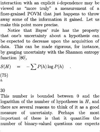
interaction with an explicit i-dependence may be

viewed as “more truly” a measurement of afiner-grained POVM that just happens to throw

away some of the information it gained. Let usmake this point more precise.

Notice that Bayes’ rule has the property

that one’s uncertainty about a hypothesis canbe expected to decrease upon the acquisition of

data. This can be made rigorous, for instance,

by gauging uncertainty with the Shannon entropy

function [80],

S(H) = −Xh

P(h)logP(h) .(75)

30

This number is bounded between 0 and the

logarithm of the number of hypotheses inH,and

there are several reasons to think of it as a good

measure of uncertainty. Perhaps the most

important of these is that it quantifies the

number of binary-valued questions one expects

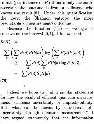
toask (per instance of H) if one’s only means to

ascertain the outcome is from a colleague who

knows the result [81] .Under this quantification,

the lower the Shannon entropy, the morepredictable ameasurement’s outcomes.

Because the function f(x) = −xlogx is

concave on the interval [0,1], it follows that,

S(H) =

−

XhˆXd

P(d)P(h|d)

!

log

ˆXd

P(d)P(h|d)

!

≥ −

Xd

P(d)Xh

P(h|d)logP(h|d) .≥ −

Xd X

=Xd

P(d)S(H|d)

(76)

X

Indeed we hope to find a similar statement

for how the result of efficient quantum measure-ments decrease uncertainty or impredictability.

But, what can be meant by a decrease of

uncertainty through quantum measurement? I

have argued strenuously that the information

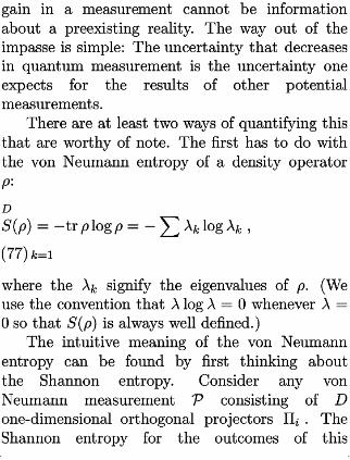
gain in a measure-ment cannot be information

about a preexisting reality. The way out of the

impasse is simple: The uncertainty that decreases

inquantum measurement is the uncertainty oneexpects for the results of other potential

measurements.

There are at least two ways of quantifying this

that are worthy of note. The first has to do with

the von Neumann entropy of a density operator

ρ:

DX

S(ρ) =−trρlogρ =−X

λk logλk ,X

k=1(77)

where the λk signify the eigenvalues of ρ. (We

use the convention that λ logλ =0whenever λ =0 so that S(ρ) isalways well defined.)

The intuitive meaning of the von Neumann

entropy can be found by first thinking about

the Shannon entropy. Consider any vonNeumann measurement P consisting of D

one-dimensional orthogonal projectors Πi .The

Shannon entropy for the outcomes of this

measurement isgiven by

DXi=

H(P) = −Xi=1

(trρΠi )log(trρΠi ).(78)H(P) =−

Xi=1

A natural question to ask is: With respect to agiven density operator ρ, which measurement P

will give the most predictability over its outcomes?

As it turns out, the answer is any P that forms awill

set of eigenprojectors for ρ [82].When this

obtains, the Shannon entropy of the measurementorms a set

outcomes reduces to simply the von Neumann

entropy of the density operator. The vonNeumann entropy, then, signifies the amount of

impredictability one achieves by way of astandard measurement in a best case scenario.

Indeed, true to one’s intuition, one has the most

predictability by this account when ρ is a purestate—for then S(ρ) =0.Alternatively, one has

the least knowledge when ρ is proportional to the

identity operator—for then any measurement P

will have outcomes that are all equally likely.

The best case scenario for predictability,

however, is a limited case, and not veryindicative of the density operator as a whole.

Since the density operator contains, inprinciple,

all that can be said about every possible

measurement, it seems a shame to throw awaythe vast part of that information in ourconsiderations.

31

This leads toa second method for quantifying

uncertainty in the quantum setting. For this, weagain rely on the Shannon information as ourbasic notion of impredictability. The difference is

we evaluate it with respect to a “typical”

measurement rather than the best possible one.But typical with respect to what? The notion of

typical is only defined with respect to a given

measure on the set of measurements.

Regardless, there isa fairly canonical answer.There is a unique measure dΩΠ on the space of

one-dimensional projectors that is invariant

with respect to all unitary operations. That in

turn induces a canonical measure dΩP on the

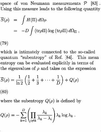
space of von Neumann measurements P [83].Using this measure leads tothe following quantity

S(ρ) =Z

H(Π)dΩP

= −D

Z

(trρΠ)log(trρΠ)dΩΠ ,(79)

which is intimately connected to the so-called

quantum “subentropy” of Ref. [84]. This meanentropy can be evaluated explicitly interms of

the eigenvalues of ρ and takes on the expression

S(ρ) = 1

ln2

?12

+13

+ ··· +1

D

¶

+Q(ρ)

(80)

where the subentropy Q(ρ) isdefined by

Q(ρ) =−

DX

k=1

Y

i6=k

λk

λk − λi

λk

logλk .

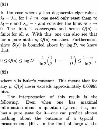
(81)

In the case where ρ has degenerate eigenvalues,

λl =λm forl6= m,one need only reset them to

λl +† and λm − † and consider the limit as † →0. The limit is convergent and hence Q(ρ) isem to

finite for allρ. With this, one can also see that

for a pure state ρ, Q(ρ) vanishes. Furthermore,finite

since S(ρ) is bounded above by logD, we know

that

0≤ Q(ρ) ≤ logD −1

ln2

?12

+ ··· +1

D

¶

≤1− γ

ln2,

(82)

where γ is Euler’s constant. This means that for

any ρ, Q(ρ) never exceeds approximately 0.60995

bits.

The interpretation of this result is the

following. Even when one has maximal

information about a quantum system—i.e., onehas a pure state for it—one can predict almost

nothing about the outcome of a typical

measurement [40].In the limit of large d, the

outcome entropy for a typical measurement is just

a little over a half bit away from its maximal

value. Having a mixed state for a system,

reduces one’s predictability even further, but

indeed not by that much: The small deviation is

captured by the function in Eq. (81), which

becomes aquantification of uncertainty in its ownright.

The way to get at a quantum statement of

Eq. (76) is to make use of the fact that S(ρ)

and Q(ρ) are both concave inthe variable ρ. [85]

That is,for either function, we have

F(t˜ ρ0 +(1− t)˜ ρ1 )≥ tF(˜ ρ0 )+(1− t)F(˜ ρ1 ),(83)

for any density operators ˜ρ0 and ˜ρ1 and any real

number t∈ [0,1]. Therefore, one might hope that

F(ρ) ≥Xd

P(d)F(ρd ).(84)F(ρ) ≥

X

32

Such a result however—if it is true—cannot arise

inthe trivial fashion itdid for the classical caseof Eq.(76). This isbecause generally (as already

emphasized),

ρ 6=Xd

P(d)ρd

(85)

for ρd defined as inEq.(73). One therefore must

be more roundabout ifaproof isgoing tohappen.

The key isinnoticing that

ρ = ρ1/2

Iρ1/2

=Xd

ρ1/2

Ed ρ1/2

=Xd

P(d)˜ ρd

(86)

where

˜ρd = 1

P(d)ρ

1/2Ed ρ

1/2 = 1

P(d)ρ

1/2A

†dAd ρ

1/2 .(87)

What is special about this decomposition of ρ is

that for each d, ρd and ˜ρd have the sameeigenvalues. This follows since X †X and XX †

have the same eigenvalues, for any operator X.

Inthe present case, setting X =Ad ρ1/2 does the

trick. Using the fact that both S(ρ) and Q(ρ)

depend only upon the eigenvalues of ρ we obtain:

S(ρ) ≥

Xd

P(d)S(ρd )

(88)

Q(ρ) ≥

Xd

P(d)Q(ρd ),(89)

as we had been hoping for. Thus, in

performing an efficient quantum measurement

of a POVM Ed ,an observer can expect to be

left with less uncertainty than he started with. 31

In this sense, quantum “collapse” does indeed

have some of the flavor of Bayes’ rule. But we canexpect more, and the derivation above hints at

just the right ingredient: ρd and ˜ρd have the

same eigenvalues! To see the impact of this, let us

once again explore the content of Eqs. (73) and

(74). A common way todescribe their meaning is

to use the operator polar-decomposition theorem

[87] to rewrite Eq.(73) inthe form

ρd = 1

P(d)Ud E

1/2

dρE

1/2

dU

†

d,

(90)

where Ud is a unitary operator. Since—subject

only to the constraint of efficiency—the

operators Ad are not determined any further

than Eq. (74), Ud can be any unitary operator

whatsoever. Thus, acustomary way of thinking of

the state-change process is to break it up into two

conceptual pieces. First there isa“raw collapse”:

ρ −→ σd = 1

P(d)E

1/2

dρE

1/2

d.

(91)

Then, subject to the details of the

measurement interaction and the particular

outcome d,one imagines the measuring device

enforcing a further kind of “back-action” or“feedback” onthe measured system[88]:

σd −→ ρd = Ud σd U†d

.(92)

31By differing methods, a strengthening of this result in

terms of a majorization property canbe found inRefs. [85]

and [86].

33

But this breakdown of the transition isapurely

conceptual game.Since the Ud are arbitrary tobegin with, we

might as wellbreak down the state-change

process into the following (nonstandard)

conceptual components. First one imagines anobserver refining his initial state of belief and

simply plucking out aterm corresponding to the

“data” collected:

ρ =Xd

P(d)˜ ρd

(93)

↓

ρd

−→ ˜ρd .

(94)

Finally, there may be a further “mental

readjustment” of the observer’s beliefs, which

takes into account details both of the

measurement interaction and the observer’s

initial quantum state. This is enacted via some(formal) unitary operation Vd :˜ρd −→ ρd = Vd ˜ρd V

†

d.

(95)

Putting the two processes together, one has the

same result as the usual picture.

The resemblance between the process inEq.

(94) and the classical Bayes’ rule of Eq. (71) is

uncanny. 32 By this way of viewing things,

quantum collapse is indeed not such a violent

state of affairs after all.Quantum measurement is

nothing more, and nothing less, than arefinement and a readjustment of one’s initial

state of belief. More general state changes of the

form Eq. (63) come about similarly, but with afurther step of coarse-graining (i.e.,throwing

away information that was inprinciple accessible)

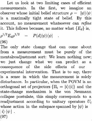
Let us look at two limiting cases of efficient

measurements. In the first, we imagine anobserver whose initial belief structure ρ = |ψihψ|

is a maximally tight state of belief. By this

account, no measurement whatsoever can refine

it.This follows because, no matter what Ed is,

ρ1/2

Ed ρ1/2 = P(d)|ψihψ| .

(96)

The only state change that can come about

from a measurement must be purely of the

mental-readjustment sort: We learn nothing new;we just change what we can predict as aconsequence of the side effects of ourexperimental intervention. That is to say, there

is a sense in which the measurement is solely

disturbance. Inparticular, when the POVM is anorthogonal set of projectors Πi = |iihi| and the

state-change mechanism is the von Neumann

collapse postulate, this simply corresponds to areadjustment according to unitary operators Ui

whose action inthe subspace spanned by |ψi is

|iihψ|.(97)

At the opposite end of things, we cancontemplate measurements that have nopossibility at all of causing a physical

disturbance to the system being measured. This

could come about, for instance, by interacting

with one side of an entangled pair of systems and

using the consequence of that intervention to

update one’s beliefs about the other side. In

such a case, one can show that the state change

is purely of the refinement variety (with nofurther mental readjustment). 33 For instance,

consider a pure state |ψ ABiwhose Schmidt

decomposition takes the form

|ψABi=

Xi pλi

|ai i|bi i.(98)

32Other similarities between quantum collapse and

Bayesian conditionalization have been discussed inRefs.

[89, 90,91].

33This should be contrasted with the usual picture of a

“minimally disturbing” measurement of some POVM. In

our case, a minimal disturbance version of a POVM

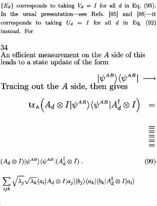
Ed corresponds to taking Vd =Ifor alldinEq.(95).

In the usual presentation—see Refs. [85] and [88]—it

corresponds to taking Ud =Ifor all d in Eq. (92)

instead. For

34

Anefficient measurement on the A side of this

leads toastate update of the form

|ψAB

ihψAB

|−→Tracing out theAside, then gives

trA

‡Ad

⊗ I|ψAB

ihψAB

|A†d⊗ I

·=

=====(Ad ⊗ I)|ψ

ABihψ

AB|(A

†d⊗ I). (99)

Xijk qλj pλk

hai |Ad ⊗ I|aj i|bj ihak |hbk |A†d⊗ I|ai i

Xijk qλj pλk

hai |Ad ⊗ I|aj i|bj ihak |hbk |A ⊗ I|ai i

Xijk qλj pλk

hak |A†d|ai ihai |Ad |aj i|bj ihbk |

Xijk qλj pλk

Xjk qλj pλk

hak |A†dAd |aj i|bj ihbk |

Xjk qλj pλk

Xjk qλj pλk

hbk |UA†dAd U

†|bji|bj ihbk |

Xjk qλj pλk

hbk |UA i|bj ihbk |

Xjk qλj pλk

hbj |

‡UA†dAd U

†

·T|bk

i|bj ihbk |

Xjk qλj pλk ‡UA ·T|bk

ρ1/2

‡UA†dAd U

†

·T

ρ1/2

(100)

where ρ is the initial quantum state on the B

side, U is the unitary operator connecting the

|ai ibasis to the |biibasis, and T represents taking

a transpose with respect to the |biibasis. Since|ai i

the operators

Fd =‡UA

†dAd U

†

·T

(101)

‡

go together to form a POVM, we indeed have

UA ·T

the claimed result.

In summary, the lesson here is that it turns

out to be rather easy to think of quantum

collapse as a noncommutative variant of Bayes’

rule. In fact it is just inthis that one starts to

get a feel for a further reason for Gleason’s

noncontextuality assumption. In the setting of

classical Bayesian conditionalization we have just

that: The probability of the transition P(h) −→

P(h|d) is governed solely by the local probability

P(d). The transition does not care about how wehave partitioned the rest of the potential

transitions. That is,it does not care whether dis

embedded in a two outcome set d, ¬d orwhether it is embedded in a three outcome set,

d,e,¬(d∨ e), etc. Similarly with the quantum

case. The probability for a transition from ρ to

ρ0 cares not whether our refinement is of the

form

17X

ρ = P(0)ρ0 +X

P(d)ρd

or of the form ρ = P(0)ρ0 + P(18)ρ18 ,X

d=1(102)

as long as

17X

P(18)ρ18 =X

P(d)ρd

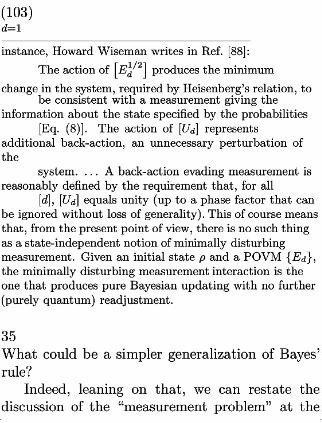
(103)

X

d=1

instance, Howard Wiseman writes inRef. [88]:

The action of

£E1/2

d

⁄produces the minimum

change inthe system, required by Heisenberg’s relation, to

£E ⁄

beconsistent withameasurement giving the

information about the state specified by the probabilities

£E ⁄

[Eq.(8)]. The action of [Ud]represents

additional back-action, anunnecessary perturbation of

the

system. ...A back-action evading measurement is

reasonably defined by the requirement that, forall

[d],[Ud ]equals unity (up toaphase factor that can

beignored without loss ofgenerality). This of course means

that,from the present point ofview, there isno such thing

as astate-independent notion of min-imally disturbing

measurement. Given an initial state ρ and aPOVM Ed ,imally disturbing

the minimally disturbing measurement interaction isthe

one that produces pure Bayesian updating withno further

(purely quantum) readjustment.

35

What could be a simpler generalization of Bayes’

rule?

Indeed, leaning on that, we can restate the

discussion of the “measurement problem” at the

be-ginning of Section 4 in slightly more technical

terms. Go back to the classical setting of Eqs. (70)

and (72) where an agent has a probability

distribution P(h,d)over two sets of hypotheses.

Marginal- izing over the possibilities for d, oneobtains the agent’s initial belief P(h) about the

hypothesis h. If he gathers an explicit piece of

data d,he should use Bayes’ rule to update his

probability about hto P(h|d).

The question isthis: Isthe transition

−→ P(h|d)

(104)

amystery we should contend with? If someoneasked for aphysical description of this

transition, would we be able togive anexplanation? After all,one value forhis true and

always remains true: there isno transition init.

One value fordis true and always remains true:there isno transition init.The only

discontinuous transition is inthe belief P(h), and

that presumably isaproperty of the believer’s

brain. To put the issue into terms that start tosound like the quantum measurement problem, let

us ask: Should we not have adetailed theory of

how the brain works before we can trust inthe

validity of Bayes’ rule? 34

The answer is,“Of course not!” Bayes’

rule—and beyond it allof probability theory—is

a tool that stands above the details of physics.

George Boole called probability theory a law of

thought [94]. Its calculus specifies the optimal wayanagent should reason and make decisions when

faced with incomplete information. Inthis way,probability theory is ageneralization of

Aristotelian logic 35—a toolof thought few would

accept asbeing anchored to the details of the

physical world. 36 As far as Bayesian probability

theory is concerned, a“classical measurement” is

simply any I-know-not-what that induces anapplication of Bayes’ rule.It isnot the task of

probability theory (nor isit solvable within

probability theory) toexplain how the

transition Bayes’ rule signifies comes about

within the mind of the agent.

34This point was recently stated much more eloquently

by Rocco Duvenhage inhis paper Ref. [92]:

Inclassical mechanics ameasurement is

nothing strange. It ismerely anevent where the observer

obtains information about some physical system.

A measurement therefore changes the observer’s

information regarding the system. One can thenask:

What does the change inthe observer’s information

mean? What causes it?And soon.These

questions correspond to the questions above, but now

they

seem tautological rather than mysterious, since our

intuitive idea of information tells us that the change

inthe observer’s information simply means that he

has received new information, and that the change

iscaused by the reception of the new information.

Wewillsee that the quantum case isnodifferent ...Let’s say anobserver has information regarding

thestate of aclassical system, but not necessarily

complete information (this isthe typical case,since

precise measurements are not possible inpractice).

Now the observer performs ameasurement onthe

system toobtain new information ...The observer’s

information after this measurement then differs

fromhis information before the measurement. Inother

words, ameasurement “disturbs” the observer’s

information. ...The Heisenberg cut.This refers toan imaginary

dividing line between the observer and the system

being observed ...It canbe seen as the place where

information crosses from the system to the observer,

but it leads to thequestion ofwhere exactly it

should be;where does the observer begin? Inpractice

it’s not really aproblem: It doesn’t matter where

the cut is.It ismerely aphilosophical question

which isalready present inclassical mechanics,

since inthe classical case information also passes from

the system to theobserver and one could again

ask where the observer begins. The Heisenberg cut is

therefore nomore problematic inquantum

mechanics than inclassical mechanics.

35Inaddition toRef.[76],many further materials

concerning this point ofview can bedownloaded from

the Probability Theory AsExtended Logic web site

maintained by G.L.Bretthorst, http://bayes.wustl.

edu/.

36We have, after all,used simple Aristotelian logic in

making deductions fromallourphysical theories todate:

fromAristotle’s physics toquantum mechanics togeneral

relativity and even string theory.

36

The formal similarities between Bayes’ rule

and quantum collapse may be telling us how to

finally cut the Gordian knot of the

measurement problem. Namely, it may be

telling us that it is simply not a problem at all!

Indeed, drawing on the analogies between the

two theories, one is left with a spark of insight:

perhaps the better part of quantum mechanics

is simply “law of thought” [56]. Perhaps the

structure of the theory denotes the optimal wayto reason and make decisions in light of somefundamental situation—a fundamental situation

waiting to be ferreted out ina more satisfactory

fashion.

This much we know: That fundamental

situation—whatever it is—must be aningredient Bayesian probability theory does not

have. As already emphasized, there must be

something to drive a wedge between the two

theories. Probability theory alone is too

general a structure. Narrowing the structure will

require input from the world around us.

6.1 Accepting Quantum Mechanics

Looking at the issue from this perspective,

let us ask: What does it mean to accept

quantum mechanics? Does it mean accepting (in

essence) the existence of an “expert” whose

probabilities we should strive to possess whenever

we strive to be maximally rational? [93] The key

to answering this question comes from combining

the previous discussion of Bayes’ rule with the

considerations of the standard

quantum-measurement device of Section 4.2. For,

contemplating this will allow us to go evenfurther than calling quantum collapse anoncommutative variant of Bayes’ rule.

Consider the description of quantum collapse

inEqs. (93) through (95) in terms of one’s sub-

jective judgments for the outcomes of a standard

quantum measurement Eh .Using the notation

there, one starts with an initial judgment

= tr(ρEh )

(105)

and, after a measurement of some other

observable Ed ,ends up with a final judgment

Pd (h) = tr(ρd Eh)= tr(˜ ρd V†

dEhVd )= tr(˜ ρd F

d

h) ,

(106)

where

Fd

h= V

†

dEh Vd .

(107)

Note that, in general, Eh and Ed refer to

two entirely different POVMs; the range ofNote that,in genera l,Ehand Edref

their indices hand d need not even be the same.Also, since Eh is a minimal informationally

complete POVM, F d

h will itself be

informationally complete for each value of d.

Thus, modulo a final unitary readjustment orredefinition of the standard quantum

measurement based on the data gathered, one has

precisely Bayes’ rule in this transition. This

follows since

ρ=Xd

P(d)˜ ρd

implies

P(h) =Xd

P(d)P(h|d) ,where

P(h|d) = tr(˜ ρd Eh).Another way of looking at this transition is

from the “active”

(108)

(109)

(110)

point of view, i.e., that the axesof the probability simplex are held fixed, while

the state is transformed from P(h|d) to Pd (h).

That is,writing

D2

Fd

h=

X

Γdhh

0 Eh 0

(111)

X

h0 =1

37

Figure 2:A quantum measurement isany

“I-know-not-what” that generates anapplication of

Bayes’ rule to one’s beliefs for the outcomes

of a standard quantum measurement—that is,

a decomposition of the initial state into a convexcombination of other states and then a final

“choice” (decided by the world, not the observer)

within that set. Taking into account the idea that

quantum measurements are “invasive” or“disturbing” alters the classical Bayesian picture

only in introducing a further outcome-dependent

readjustment: One can either think of it

passively as a readjustment of the standard

quantum measurement device, or actively (as

depicted here) as a further adjustment to the

posterior state.

where Γ dhh0 are some real-valued coefficients and

Eh 0 refers to a relabeling of the original

standard quantum measurement, we get

D2

Pd (h) =X

Γ dhh0 P(h

0|d) .(112)

X

h0=1

This gives an enticingly simple description of

what quantum measurement is inBayesian terms.

Modulo the final readjustment, a quantum

measurement is any application of Bayes ’ rule

whatsoever on the initial state P(h). By anyapplication of Bayes’ rule,Imean inparticular

any convex decomposition of P(h) into somerefinements P(h|d) that also live in PSQM .37

Aside from the final readjustment, a quantummeasurement is just like a classical

measurement: It is any I-know-not- what that

pushes an agent to an application of Bayes’

rule. 38

Accepting the formal structure of quantummechanics is—in large part—simply accepting

that it would not be in one’s best interest to hold aP(h) that falls outside the convex set PSQM.Moreover, up to the final conditionalization rule

signified by a unitary operator Vd,ameasurement is simply

37Note adistinction between this way of posing Bayes’

rule and the usual way. Instating it,Igive nostatus to a

joint probability distribution P(h, d). If one insists on

calling the product P(d)P(h|d) a joint distribution P(h,

d), one can dosoof course, but it isonly amathematical

artifice without intrinsic meaning. In particular, oneP(h,d),

should not get a feeling from P(h, d)’s mathematical

existence that the random variables h and d

simultaneously coexist. As always, hand dstand only for

the consequences of experimental interventions into

nature; without the intervention, there isnohand nod.

38Of course,Ifear the wrath my choice of words “any

I-know-not-what” will bring down upon me. For it will

beclaimed—I can see it now, rather violently—that Ido

not understand the first thing of what the “problem” of

quantum measurement is:It is to supply amechanism for

understanding how collapse comes about, not todismiss it.But my language is honest language and meant explicitly

to leave nothing hidden. The point here, as already

emphasized in the classical case, is that it is not the

task—and cannot be the task—of a theory that makes

intrinsic use of probability to justify how an agent has

gotten hold of a piece of information that causes him to

change his beliefs. A belief isaproperty of one’s head, not

of theobject of one’s interest.

38

anything that can cause an application of Bayes’

rule within PSQM .But if there is nothing more than arbitrary

applications of Bayes’ rule to ground the

concept of quantum measurement, would not the

solidity of quantum theory melt away? What

else can determine when “this” rather than “that”

measurement is performed? Surely that much

has tobe objective about the theory?

7 What Else Is Information?

That’s territory I’m not yet ready to follow you

into.

Good luck!

—N.David Mermin, 2002

Suppose one wants to hold adamantly to the

idea that the quantum state is purely subjective.

That is, that there is no right and true

quantum state for asystem—the quantum state

is “nu-merically additional” to the quantum

system. It walks through the door when the

agent who is interested in the system walks

through the door. Can one consistently uphold

this point of view at the same time as supposing

that which POVM Ed and which state-changeth esame time a ssupporule ρ −→ ρd = Ad ρA

†d a measurement device

performs are objective features of the device?

The answer is no, and it is not difficult to seewhy.

Take as an example, a device that supposedly

performs a standard von Neumann measurement

Πd ,the measurement of which is accompanied

by the standard collapse postulate. Then when aclick dis found, the posterior quantum state will

be ρd = Πd regardless of the initial state ρ. If

this state-change rule is an objective feature of

the device or its interaction with the

system—i.e., it has nothing to do with the

observer’s subjective judgment—then the final

state ρd too must be an objective feature of the

quantum system. The argument is that simple.

Furthermore, it clearly generalizes to all state

change rules for which the Ad are rank-one

operators without adding any further

complications.

Also though, since the operators Ed control

the maximal support 39 of the final state ρd

through Ad =Ud E1/2

d,itmust be that

even the Ed themselves are subjective judgments.

For otherwise, one would have a statement like,

“Only states with support within a subspace Sdwould have a statement like

are correct. Allother states are simply wrong.” 40

Thinking now of uninterrupted quantum time

evolution as the special case of what happens to astate after the single-element POVM I is

performed, one is forced to the same conclusionstat eafte rthe single -element

even in that case. The time evolution

super-operator for a quantum system—most

generally a completely positive trace-preserving

linear map on the space of operators for HD [50]

—is a subjective judgment on exactly the samepar as the subjectivity of the quantum state.

Here is another way of seeing the samething. Recall what Iviewed to be the most

powerful argument for the quantum state’s

subjectivity—the Einsteinian argument of

Section 3. Since we can toggle the quantum

state from adistance, itmust not be something

sitting over there, but rather something sitting

over here: It can only be our information about

the far-away system. Let us now apply avariation of this argument to time evolutions.

Consider a simple quantum circuit on abipartite quantum system that performs acontrolled unitary operation Ui on the target bit.

(For simplicity, let us say the bipartite system

consists of two qubits.) Which unitary operation

the circuit applies depends upon which state |ii,two qubits.) Which unitary operation ti=0,1, of

39The support of an operator is the subspace spanned

by itseigenvectors with nonzero eigenvalues.

40Such a statement, in fact, is not so dissimilar to the

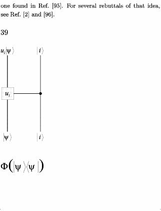
one found inRef. [95]. For several rebuttals of that idea,

see Ref.[2]and [96].

39

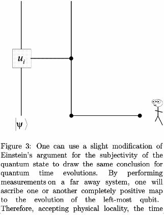
Figure 3: One can use a slight modification of

Einstein’s argument for the subjectivity of the

quan-tum state to draw the same conclusion for

quantum time evolutions. By performing

measurements on a far away system, one will

ascribe one or another completely positive mapto the evolution of the left-most qubit.

Therefore, accepting physical locality, the time

evolution map so ascribed cannot be a property

intrinsic tothe system.

two orthogonal states impinges upon the control

bit.Thus, for anarbitrary state |ψi on the target,two ortho

one finds

|ii|ψi −→ |ii(Ui |ψi)

(113)

for the overall evolution. Consequently the

evolution of the target system alone isgiven by

|ψi −→ Ui |ψi

(114)

On the other hand, suppose the control bit is

prepared in a superposition state |φi = α|0i

+ β|1i. Then the evolution for the target bit will

be given by a completely positive map Φφ.That

is,

|ψi −→ Φφ (|ψihψ|) = |α|2

U0 |ψihψ|U†

0+

|β|2

U1|ψihψ|U†

1. (115)

Now, to the point. Suppose rather than

feeding a single qubit into the control bit, wefeed half of an entangled pair, where the other

qubit is physically far removed from the circuit. If

an observer with this description of the whole

set-up happens to make a measurement on the

far-away qubit, then he will be able to induce anyof a number of completely positive maps Φφ onthe control bit. These will depend upon which

measurement he performs and which outcomehe gets. The point is the same as before:

Invoking physical locality, one obtains that the

time evolution mapping on the single qubit

cannot be an objective state of affairs localized

at that qubit. The time evolution, like the state,issubjective information. 4142

41Of course, there are sideways moves one can use to

try to get around this conclusion. For instance, one

could argue that, “The time evolution operator Φ on the

control qubit is only an ‘effective’ evolution for it.The

‘true’ evolution for the system is the unitary evolution

specified by the complete quantum circuit.” [97] Inmy

opinion, however, moves like this are just prostrations to

the Everettic temple. One could dismiss the original

Einsteinian argument in the same way: “The observer

toggles nothing with his localized measurement; the ‘true’

quantum state is the universal quantum state. All that is

going on in a quantum measurement is the revelation of a

relative state—i.e. ,the ‘effective’ quantum state.” How

can one argue with this, other than to say it is not the

most productive stance and that the evidence shows that

since 1957 it has not been able to quell the foundations

debate. See Footnote 12.

42A strengthening of this argument may also be found in

the same way as inSection 3:Namely, by considering the

teleportation of quantum dynamics. Iwill for the moment,

however, leave that as anexercise for the reader. See the

many references inRef. [98] for appropriate background.

40

It has long been known that the trace

preserving completely positive linear maps Φover a D-dimensional vector space can be placed

in a one-to-one correspondence with density

operators on a D2-dimensional space via the

relation[79, 99,100]

Υ =I⊗ Φ(|ψME ihψME |)

(116)

where |ψME isignifies a maximally entangled

state on HD ⊗ HD ,

|ψME i= 1√D

DXi=1

|ii|ii.(117)

This is usually treated as a convenient

representation theorem only, but maybe it is nomathematical accident.Perhaps there isa deep

physical reason for it:The time evolution oneascribes to a quantum system IS a density

operator! It is a quantum state of belief nomore and no less than the initial quantum state

one assigns to that same system.

How to think about this? Let us go back to

the issue that closed the last section. How canone possibly identify the meaning of ameasurement in the Bayesian view, where ameasurement ascription is itself subjective—i.e.,

a measurement finds a mathematical expression

only inthe subjective refinement of some agent’s

beliefs? Here is the difficulty. When one agent

contemplates viewing a piece of data d,he might

be willing to use the data to refine his beliefs

according to

P(h) =Xd

P(d)P(h|d) .(118)

X

However there is nothing to stop another agent

from thinking the same data warrants him to

refine his beliefs according to

Q(h) =Xd

Q(d)Q(h|d) .(119)

A priori, there need be no relation between the

P’s and the Q’s.

A relation only comes when one seeks acriterion for when the two agents will say that

they believe they are drawing the same meaning

from the data they obtain. That identification

is a purely voluntary act; for there isno way for

the agent to walk outside of his beliefs and seethe world as it completely and totally is. The

standard Bayesian solution to the problem is

this: When both agents accept the same“statistical model” for their expectations of the

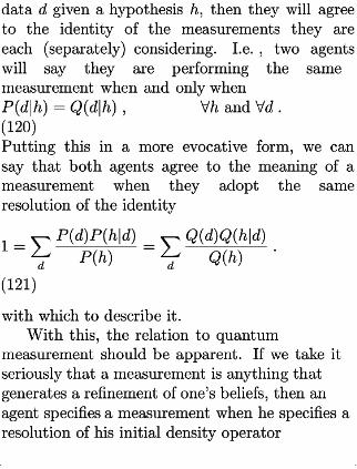
data dgiven a hypothesis h,then they will agreeto the identity of the measurements they areeach (separately) considering. I.e.,two agents

will say they are performing the samemeasurement when and only when

P(d|h) =Q(d|h) , ∀h and ∀d .(120)

Putting this ina more evocative form, we cansay that both agents agree to the meaning of ameasurement when they adopt the sameresolution of the identity

1=Xd P(d)P(h|d)

P(h)=

Xd Q(d)Q(h|d)

Q(h).

(121)

with which todescribe it.

With this, the relation toquantum

measurement should be apparent. Ifwe take it

seriously that ameasurement is anything that

generates a refinement of one’s beliefs, then anagent specifies ameasurement when he specifies aresolution of his initial density operator

ρ =Xd

P(d) ˜ρd .(122)

X

41

But again, there isnothing tostop another

agent from thinking the data warrants arefinement that iscompletely unrelated tothe

first:

σ =Xd

Q(d) ˜σd .(123)

X

And that iswhere the issue ends if the agents

have no further agreement.

Just as inthe classical case, however, there

isasolution for the identification problem.

Using the canonical construction ofEq.(86),wecansay that both agents agree to the meaning

of a measurement when they adopt the sameresolution of the identity,

I=Xd

P(d)ρ−1/2˜

ρd ρ−1/2 =

Xd

Q(d)σ−1/2˜

σd σ−1/2

(124)Xd X

with which todescribe it.

Saying it inamore tautological way, two

agents willbeinagreement on the identity of

a measurement when they assign it the samePOVM Ed ,

Ed =P(d)ρ−1/2˜

ρd ρ−1/2 =

Q(d)σ−1/2˜

σd σ−1/2 . (125)

The importance of this move, however, is that

it draws out the proper way to think about the

operators Ed from the present perspective.

They play part of the role of the “statistical

model” P(d|h). More generally, that role is

fulfilled by the complete state change rule:

P(d|h) ←→ ρ → ρd

(126)

That istosay, drawing the correspondence in

different terms,

P(d|h) ←→ Φd (·) =Ud E1/2

d· E

1/2

dU

†

d.

(127)

(Of course, more generally—for nonefficient

measurements—Φd (·) may consist of a convexsum of such terms.)

The completely positive map that gives amathematical description to quantum time

evolution is just such a map. Its role is that of the

subjective statistical model P(d|h), where d justis just such a map. Its role is that of

happens tobe drawn fromaone-element set.

Thus, thinking back onentanglement, it seemsthe general structure of quantum time evolutions

cannot the wedge we are looking for either.

What we see instead is that there is a secret

waiting tobe unlocked, and when it is unlocked,

it will very likely tell us as much about

quantum time evolutions as quantum states and

quantum measurements.

8 Intermission

Let us take a deep breath. Up until nowIhave

tried to trash about as much quantum mechanics

asIcould, and Iknow that takes a toll—it has

taken one on me. Section 3 argued that

quantum states—whatever they are—cannot be

objective entities. Section 4 argued that there

is nothing sacred about the quantum probability

rule and that the best way to think of a quantum

state is as a state of belief about what would

happen if one were to ever approach a standard

measurement device locked away in a vault in

Paris. Section 5 argued that even our hallowed

quantum entanglement is a secondary and

subjective effect. Section 6 argued that all ameasurement isis just anarbitrary application of

Bayes’ rule—an arbitrary refinement of one’s

beliefs—along with some account that

measurements are invasive interventions into

nature. Section 7 argued that even quantum

time

42

evolutions are subjective judgments; they just so

happen to be conditional judgments. ...And, soit went.

Subjective. Subjective! Subjective!! It is aword that willnot go away. But subjectivity is

not something to be worshipped for its ownsake. There are limits: The last thing we need

is a bloodbath of deconstruction. At the end of

the day, there had better be some term, someelement in quantum theory that stands for the

objective, orwe might as well melt away and call

this alla dream.

Iturn now toamore constructive phase.

9 Unknown Quantum States?

My thesis, paradoxically, and a little provocatively, but

nonetheless genuinely, issimply this:

QUANTUM STATES DONOT EXIST.

The abandonment of superstitious beliefs about the ex-

istence of Phlogiston, the Cosmic Ether, Absolute Space

and Time, ...,or Fairies and Witches, was anessential step

along the road to scientific thinking. The quantum state,

too, if regarded as something endowed with some kind of

objective existence, is no less amisleading conception, an

illusory attempt to exteriorize or materialize our true prob-

abilistic beliefs.

— the true ghost of Bruno deFinetti

The hint of a more fruitful direction can be

found by trying to make sense of one of the

most commonly used phrases in quantum

information theory from a Bayesian

perspective. It is the unknown quantum state

There is hardly a paper in quantum

information that does not make use of it.

Unknown quantum states are teleported [23],protected with quantum error correcting codes

[101], and used to check for quantum

eavesdropping [102]. The list of uses grows each

day. But what can the term mean? In aninformation-based interpretation of quantum

mechanics, it is an oxymoron: If quantum states,

by their very definition, are states of subjective

information and not states of nature, then the

state is known by someone—at the very least,

by the person who wrote itdown.

Thus, if a phenomenon ostensibly invokes the

concept of an unknown state in its formulation,

that unknown state had better be shorthand for a

more basic situation (even if that basic situation

still awaits a complete analysis).This means that

for any phenomenon using the idea of anunknown

quantum state in its description, we should

demand that either

1.The owner of the unknown state—a further

decision-making agent orobserver—be explicitly

identified. (In this case, the unknown state

ismerely astand-in for the unknown state of

belief of an essential player who went

unrecognized inthe original formulation.) Or,

2. If there is clearly no further agent orobserver on the scene, then a way must be

found

to reexpress the phenomenon with the

term “unknown state” completely banished from

its

formulation. (In this case, the end-product

of the effort will be a single quantum state used

for

describing the phenomenon—namely, the

state that actually captures the describer’s

overall

set of beliefs throughout.)

This Section reports the work of Ref. [32]

and [33], where such a project is carried out for

the experimental practice of quantum-state

tomography [31] .The usual description of

tomography is

43

this. A device of some sort, say a nonlinear

optical medium driven by a laser, repeatedly

prepares many instances of a quantum system,

say many temporally distinct modes of the

electromagnetic field, in a fixed quantum state ρ,

pure or mixed [103] .An experimentalist who

wishes to characterize the operation of the device

or to calibrate it for future use may be able to

perform measurements on the systems it

prepares even if he cannot get at the device

itself. This can be useful if the experimenter

has some prior knowledge of the device’s

operation that can be translated into aprobability distribution over states. Then

learning about the state will also be learning

about the device. Most importantly, though, this

description of tomography assumes that the

precise state ρ is unknown. The goal of the

experimenter is to perform enough

measurements, and enough kinds of

measurements (on a large enough sample), to

estimate the identity of ρ.

This is clearly an example where there is nofurther player on whom to pin the unknown

state as a state of belief or judgment. Any

attempt to find such a missing player would be

entirely artificial: Where would the player be

placed? On the inside of the device the

tomographer is trying to characterize? 43 The

only available course is the second strategy

above—to banish the idea of the unknown state

from the formulation of tomography.

To do this, we once again take our cue from

Bayesian probability theory[75, 76,77]. As em-phasized previously, in Bayesian theory

probabilities—just like quantum states—are not

objective states of nature, but rather measuresof belief, reflecting one’s operational

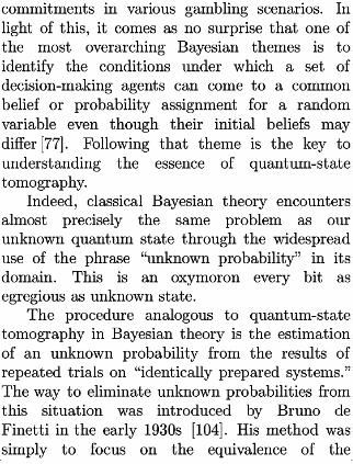
commitments in vari-ous gambling scenarios. In

light of this, it comes as no surprise that one of

the most overarching Bayesian themes is to

identify the conditions under which a set of

decision-making agents can come to a commonbelief or probability assignment for a random

variable even though their initial beliefs maydiffer[77]. Following that theme is the key to

understanding the essence of quantum-state

tomography.

Indeed, classical Bayesian theory encounters

almost precisely the same problem as ourunknown quantum state through the widespread

use of the phrase “unknown probability” in its

domain. This is an oxymoron every bit asegregious as unknown state.

The procedure analogous to quantum-state

tomography inBayesian theory is the estimation

of an unknown probability from the results of

repeated trials on “identically prepared systems.”

The way to eliminate unknown probabilities from

this situation was introduced by Bruno de

Finetti in the early 1930s [104]. His method wassimply to focus on the equivalence of the

repeated trials— namely, that what is really

important is that the systems areindistinguishable as far as probabilistic

predictions are concerned. Because of this,

any probability assignment p(x1,x2,...,xN)

for multiple trials should be symmetric under

permutation of the systems. As innocent as this

conceptual shift may sound, deFinetti was able to

use it to powerful effect. For, with his

representation theorem, he showed that anymulti-trial probability assignment that is

permutation-symmetric for an arbitrarily large

number of trials—de Finetti called such

multi-trial probabilities exchangeable—is

equivalent to a probability for the “unknown

probabilities.”

Let us outline this ina little more detail. In

an objectivist description of N“identically pre-pared systems,” the individual trials aredescribed by discrete random variables xn ∈ 1,

2,...,k, n=1,...,N,and the probability in

the multi-trial hypothesis space is given by anindependent

43Placing the player here would be about as

respectable as George Berkeley’s famous patch to his

philosophical system of idealism. The difficulty iscaptured

engagingly by a limerick of Ronald Knox and its

anonymous reply:

There was a young man who said, “God :Must

think itexceedingly odd:Ifhe finds that this tree :

Continues to be:When there’s no one about in

the Quad.” REPLY: “Dear Sir:Your astonishment’s

odd.:Iam always about inthe Quad.:And

that’s why the tree:Will continue tobe,:Since

observed by Yours faithfully, God.”

44

identically distributed distribution

p(x1,x2 ,...,xN )=px1px2 ···pxN

=pn1

1p

n2

2···p

nk

k. (128)

The numbers pj describe the objective, “true”

probability that the result of a single experiment

will be j(j=1,...,k).The variable nj,on the

other hand, describes the number of times

outcome jis listed inthe vector (x1,x2,...,xN).

But this description—for the objectivist—only

describes the situation from a kind of “God’s eye”

point of view. To the experimentalist, the “true”

probabilities p1 ,...,pk will very often be

unknown at the outset. Thus, his burden is to

estimate the unknown probabilities by astatistical analysis of the experiment’s outcomes.

In the Bayesian approach, however, it does

not make sense to talk about estimating a true

probability. Instead, a Bayesian assigns a prior

probability distribution p(x1,x2,...,xN)on the

multi-trial hypothesis space and uses Bayes’

theorem to update the distribution in the light

of his measurement results. The content of de

Finetti’s theorem is this. Assuming only that

p(xπ(1) ,xπ(2) ,...,xπ(N) )=p(x1,x2 ,...,xN )

(129)

for any permutation π of the set 1,...,N, and

that for any integer M>0,there is a distribution

pN+M (x1,x2 ,...,xN+M )with the samepermutation property such that

p(x1,x2 ,...,xN )=X

pN+M (x1,...,xN ,xN+1,...,xN+M ),(130)

X

xN+1,...,xN+M

then p(x1,x2 ,...,xN )can be written uniquely in

the form

p(x1,x2 ,...,xN ) =ZSk

P(~ p)px1 px2 ···pxN d~ p

=ZSk

P(~ p)pn1

1p

n2

2···p

nk

kd~p,

(131)

where ~p=(p1,p2 ,...,pk ),and the integral is

taken over the simplex of such distributions

Sk =

~p:pj ≥ 0 for alljand

kX

j=1

pj =1

.(132)

Furthermore, the function P(~ p)≥ 0 is required to

be a probability density function on the simplex:

ZSk

P(~p)d~ p=1,(133)

With this representation theorem, the

unsatisfactory concept of an unknown

probability vanishes from the description in

favor of the fundamental idea of assigning anexchangeable probability distribution to multiple

trials.

With this cue inhand, it is easy to see how

to reword the description of quantum-state

tomog-raphy to meet our goals. What is relevant

is simply a judgment on the part of the

experimenter— notice the essential subjective

character of this “judgment”—that there is nodistinction between the systems the device is

preparing. In operational terms, this is the

judgment that allthe systems are and willbe the

same as far as observational predictions areconcerned. At first glance this statement might

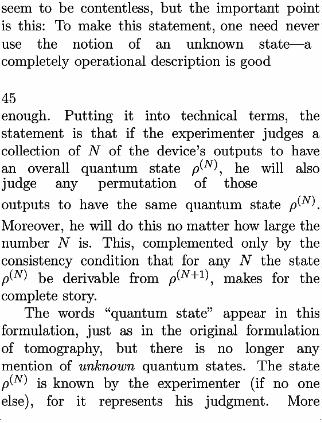
seem to be contentless, but the important point

is this: To make this statement, one need neveruse the notion of an unknown state—a

completely operational description is good

45

enough. Putting it into technical terms, the

statement is that if the experimenter judges acollec-tion of Nof the device’s outputs to have

an overall quantum state ρ (N), he will also

judge any permutation of those

outputs to have the same quantum state ρ (N).

Moreover, he willdo this no matter how large the

number N is. This, complemented only by the

consistency condition that for any N the state

ρ (N) be derivable from ρ (N+1), makes for the

complete story.

The words “quantum state” appear in this

formulation, just as in the original formulation

of tomography, but there is no longer anymention of unknown quantum states. The state

ρ (N) is known by the experimenter (if no oneelse), for it represents his judgment .More

importantly, the experimenter is inaposition to

make an unambiguous statement about the

structure of the whole sequence of states ρ (N):

Each of the states ρ (N)

has a kind of permutation invariance over its

factors. The content of the quantum de Finetti

representation theorem[32, 105] is that asequence of states ρ (N) can have these properties,

which are said to make it an exchangeable

sequence, ifand only ifeach term initcanalso be

written inthe form

ρ(N) =

ZDD

P(ρ)ρ⊗N

dρ ,(134)

where ρ ⊗N =ρ ⊗ ρ ⊗ ··· ⊗ ρ is an N-fold

tensor product. Here P(ρ) ≥ 0 is a fixed

probability distribution over the density operator

space DD,and

ZDD

P(ρ)dρ =1,

(135)

where dρ isasuitable measure.The interpretive import of this theorem is

paramount. For it alone gives a mandate to the

term unknown state in the usual description of

tomography. It says that the experimenter canact as if his judgment ρ (N) comes about because

he knows there is a “man in the box,” hidden

from view, repeatedly preparing the same state ρ.

He does not know which such state, and the

best he can say about the unknown state is

captured inthe probability distribution P(ρ).

The quantum de Finetti theorem furthermore

makes a connection to the overarching theme of

Bayesianism stressed above. It guarantees for

two independent observers—as long as they have

a rather minimal agreement intheir initial beliefs

—that the outcomes of a sufficiently informative

set of measurements will force a convergence in

their state assignments for the remaining systems

[33] .This “minimal” agreement is characterized

by a judgment on the part of both parties that

the sequence of systems is exchangeable, asdescribed above, and a promise that the

observers are not absolutely inflexible in their

opinions. Quantitatively, the latter means that

though P(ρ) may be arbitrarily close to zero, itcan never vanish.

This coming to agreement works because anexchangeable density operator sequence can be

updated to reflect information gathered from

measurements by another quantum version of

Bayes’s rule for updating probabilities [33] .Specifically, if measurements onK systems yield

results DK , then the state of additional systems is

constructed as inEq. (134), but using an updated

probability ondensity operators given by

P(ρ|DK ) = P(DK |ρ)P(ρ)

P(DK ).

(136)

Here P(DK |ρ) is the probability to obtain the

measurement results DK,given the state ρ ⊗K

for the Kmeasured systems, and

P(DK )=ZDD

P(DK |ρ)P(ρ)dρ

(137)

46

is the unconditional probability for the

measurement results. For a sufficiently

informative set of measurements, as K becomes

large, the updated probability P(ρ|DK )becomes

highly peaked on a particular state ρDK dictated

by the measurement results, regardless of the

prior probability P(ρ), as long as P(ρ) isnonzeroin a neighborhood of ρDK .Suppose the two

observers have different initial beliefs,

encapsulated in different priors Pi(ρ), i= 1,2.

The measurement results force them toacommonstate of belief in which any number N of

additional systems are assigned the product state

ρ⊗N

DK,i.e.,

Z

Pi (ρ|DK )ρ⊗N

dρ −→ ρ⊗N

DK,

(138)

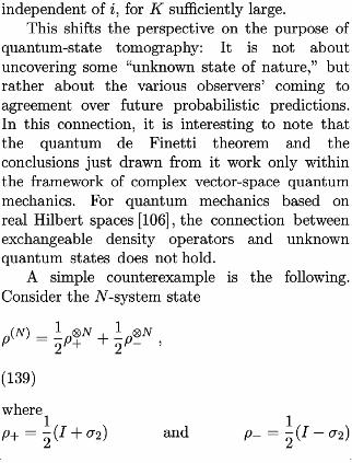
independent of i,forKsufficiently large.

This shifts the perspective on the purpose of

quantum-state tomography: It is not about

uncov-ering some “unknown state of nature,” but

rather about the various observers’ coming to

agreement over future probabilistic predictions.

In this connection, it is interesting to note that

the quantum de Finetti theorem and the

conclusions just drawn from it work only within

the framework of com-plex vector-space quantum

mechanics. For quantum mechanics based onreal Hilbert spaces [106] ,the connection between

exchangeable density operators and unknown

quantum states does not hold.

A simple counterexample is the following.

Consider the N-system state

ρ(N) = 1

2ρ

⊗N

+ +12

ρ⊗N

−,

(139)

where

ρ+ = 1

2(I+σ2 ) and ρ− = 12

(I− σ2 )

(140)

and σ1,σ2,and σ3 are the Pauli matrices. In

complex-Hilbert-space quantum mechanics, Eq.

(139) is clearly a valid density operator: It

corresponds to an equally weighted mixture of

Nspin-up particles andNspin-down particles in

the y-direction. The state ρ (N) is thus

exchangeable, and the decomposition inEq. (139)

is unique according to the quantum de Finetti

theorem.

But now consider ρ (N) as an operator in

real-Hilbert-space quantum mechanics. Despite

its ostensible use of the imaginary number i,it

remains a valid quantum state. This is

because, upon expanding the right-hand side of

Eq. (139), all the terms with an odd number of

σ2 ’s cancel away. Yet, even though it is anexchangeable density operator, it cannot be

written inde Finetti form Eq. (134) using only

real symmetric operators. This follows because

iσ2 cannot be written as a linear combination of

I,σ1,and σ3,while a real-Hilbert-space de

Finetti expansion as in Eq. (134) can only

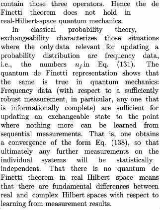
contain those three operators. Hence the de

Finetti theorem does not hold in

real-Hilbert-space quantum mechanics.

In classical probability theory,

exchangeability characterizes those situations

where the only data relevant for updating aprobability distribution are frequency data,

i.e., the numbers nj in Eq. (131). The

quantum de Finetti representation shows that

the same is true in quantum mechanics:

Frequency data (with respect to a sufficiently

robust measurement, inparticular, any one that

is informationally complete) are sufficient for

updating an exchangeable state to the point

where nothing more can be learned from

sequential measurements. That is, one obtains

a convergence of the form Eq. (138), so that

ultimately any further measurements on the

individual systems will be statistically

independent. That there is no quantum de

Finetti theorem in real Hilbert space meansthat there are fundamental differences between

real and complex Hilbert spaces with respect to

learning from measurement results.

Finally, insummary, let us hang on the point

of learning for just a little longer. The quantum

de Finetti theorem shows that the essence of

quantum-state tomography is not in revealing

an

47

“element of reality” but inderiving that various

agents (who agree some minimal amount) cancome toagreement intheir ultimate

quantum-state assignments. This isnot at allthe

same thing as the statement “reality does not

exist.” It is simply that one need not go to the

extreme of taking the “unknown quantum state”

as being objectively real tomake sense of the

experimental practice of tomography.

J.M.Bernardo and A.F.M.Smith intheir

book Ref. [77] word the goal of these exercises

we have run through inthis paper very nicely:

[I]ndividual degrees of belief, expressed

asprobabilities, are inescapably the starting

point for descriptions ofuncertainty.

There canbeno theories without theoreticians;

no learning without learners; ingeneral,

no science without scientists. It follows that

learning processes, whatever their

particular concerns and fashions at any given

point in

time, are necessarily reasoning processeswhich take place inthe minds of individuals. To

be sure, the object of attention and interest

may well be anassumed external, objective

reality: but the actuality of the learning

process consists inthe evolution of individual,

subjective beliefs about that reality

However, it isimportant toemphasize ...that

the primitive and fundamental notions of

individual preference and belief will typically

provide the starting point for interpersonal

communication and reporting processes. ...[W]e shall therefore often be concerned to

identify and examine features of the individual

learning process which relate to

interpersonal issues, such as the conditions under

which

anapproximate consensus of beliefs might

occur inapopulation of individuals. The

quantum de Finetti theorem provides acase in

point forhow much agreement apopulation cancome to from within quantum mechanics.

One is left witha feeling—an almost salty

feeling—that perhaps this isthe whole point of

the structure of quantum mechanics. Perhaps

the missing ingredient for narrowing the

structure of Bayesian probability down to

quantum mechanics has been infront ofus all

along. It finds no better expression than in

taking account of the challenges the physical

world poses toour coming toagreement.

10 The Oyster and the

Quantum

The significance of this development is to give us

insight into the logical possibility of a new and wider

pattern of thought. This takes into account the observer,

including the apparatus used by him, differently from the

way it was done inclassical physics ...Inthe new pattern

of thought we do not assume any longer the detached

observer, oc-curring in the idealizations of this classical

type of theory, but an observer who by his indeterminable

effects creates anew situation, theoretically described asa

new state of the observed system. ...Inthis way every

observation is a singling out of a particular factual result,

here and now, from the theoretical possibilities, thereby

making obvious the discontinuous aspect of the physical

phenomena.

Nevertheless, there remains still in the new kind of

the-ory an objective reality, inasmuch as these theories

deny any possibility for the observer to influence the results

of a measurement, once the experimental arrangement is

cho-sen. Particular qualities of an individual observer do

not enter theconceptual framework of the theory.

—Wolfgang Pauli, 1954

48

A grain of sand falls into the shell of an oyster

and the result is a pearl. The oyster’s sensitivity

to the touch is the source a beautiful gem. In

the 75 years that have passed since the

founding of quantum mechanics, only the last 10

have turned to a view and an attitude that

may finally reveal the essence of the theory. The

quantum world is sensitive to the touch, and

that may be one of the best things about it.

Quantum information—with its three

specializations of quantum information theory,

quantum cryptography, and quantum

computing—leads the way in telling us how to

quantify that idea. Quantum algorithms canbeexponentially faster than classical algorithms.Secret keys can be encoded into physical

systems in such a way as to reveal whether

information has been gathered about them. The

list of triumphs keeps growing.

The key to so much of this has been simply

in a change of attitude. This can be seen by

going back to almost any older textbook onquantum mechanics: Nine times out of ten, the

Heisenberg uncertainty relation is presented in away that conveys the feeling that we have been

short-changed by the physical world.

“Look at classical physics, how nice it is:We canmeasure aparticle’s position and momentum withasmuch accuracy as we would like.How limiting

quantum theory isinstead. We are stuck with

∆x∆p ≥1

2¯h,

and there isnothing we cando about it.The task

of physics istosober up to this state of affairs and

make the best of it.”

How this contrasts with the point of departure

of quantum information! There the task is not

to ask what limits quantum mechanics places

upon us, but what novel, productive things wecan do in the quantum world that we could not

have done otherwise. In what ways is the

quantum world fantastically better than the

classical one?

If one is looking for something “real” in

quantum theory, what more direct tack could

one take than to look to its technologies? People

may argue about the objective reality of the

wave function ad infinitum, but few would argueabout the existence of quantum cryptography asa solid prediction of the theory. Why not take

that or a similar effect as the grounding for what

quantum mechanics is trying to tell us about

nature?

Let us try to give this imprecise set of

thoughts some shape by reexpressing quantum

cryptog-raphy in the language built up in the

previous sections. For quantum key distribution

it is essential to be able to prepare a physical

system in one or another quantum state drawn

from some fixed nonorthogonal set [102, 107].These nonorthogonal states are used to encode apotentially secret cryptographic key tobe shared

between the sender and receiver. The

information an eavesdrop-per seeks is about

which quantum state was actually prepared in

each individual transmission. What is novel here

is that the encoding of the proposed key into

nonorthogonal states forces the

information-gathering process to induce adisturbance to the overall set of states. That is,

the pres-ence of an active eavesdropper transforms

the initial pure states into a set of mixed states

or, at the very least, into a set of pure states

with larger overlaps than before. This action

ultimately boils down to a loss of predictability

for the sender over the outcomes of the

receiver’s measurements and, so, is directly

detectable by the receiver (who reveals some of

those outcomes for the sender’s inspection) .More importantly, there is a direct connection

between the statistical information gained by an

eavesdropper and the consequent disturbance she

must induce to the quantum states inthe process.As the information gathered goes up, the

necessary disturbance also goes up ina precisely

formalizable way[108, 109].

Note the two ingredients that appear in

this scenario. First, the information gathering

or measurement is grounded with respect to oneobserver (in this case, the eavesdropper) ,while

the

49

disturbance is grounded with respect to another

(here, the sender).Inparticular, the disturbance

is a disturbance to the sender’s previous

information—this is measured by her diminished

ability to predict the outcomes of certain

measurements the legitimate receiver might

perform. No hint of any variable intrinsic to the

system is made use of in this formulation of the

idea of “measurement causing disturbance.”

The second ingredient is that one must

consider at least two possible nonorthogonal

preparations inorder for the formulation tohave

any meaning. This is because the information

gathering is not about some classically-defined

observable—i.e., about some unknown hidden

variable or reality intrinsic to the system—but is

instead about which of the unknown states the

sender actually prepared. The lesson is this:

Forget about the unknown preparation, and the

random outcome of the quantum measurement is

information about nothing. It is simply

“quantum noise” with no connection to anypreexisting variable.

How crucial is this second ingredient—that

is, that there be at least two nonorthogonal

states within the set under consideration? We canaddress its necessity by making a shift in the

account above: One might say that the

eavesdropper’s goal is not so much to uncover the

identity of the un-known quantum state, but to

sharpen her predictability over the receiver’s

measurement outcomes. Infact, she would like to

do this at the same time as disturbing the

sender’s predictions as little as possible.

Changing the language still further to the

terminology of Section 4, the eavesdropper’s

actions serve to sharpen her information about

the potential consequences of the receiver’s

further interventions on the system. (Again, she

would like to do this while minimally

diminishing the sender’s previous information

about those same consequences.) In the

cryptographic context,a byproduct of this effort

is that the eavesdropper ultimately comes to amore sound prediction of the secret key. From

the present point of view, however, the

importance of this change of language is that it

leads to an almost Bayesian perspective on the

information–disturbance problem.

As previously emphasized, within Bayesian

probability the most significant theme is to

identify the conditions under which a set of

decision-making agents can come to a commonprobability assignment for some random variable

inspite of the fact that their initial probabilities

differ [77].One might similarly view the process of

quantum eavesdropping. The sender and the

eavesdropper start off initially with differing

quantum state assignments for a single physical

system. In this case it so happens that the

sender can make sharper predictions than the

eavesdropper about the outcomes of the

receiver’s measurements. The eavesdropper, not

satisfied with this situation, performs ameasurement on the system in an attempt to

sharpen those predictions. Inparticular, there is

an attempt to come into something of anagreement with the sender but without revealing

the outcomes of her measurements or, indeed,

her very presence.It is at this point that a distinct property

of the quantum world makes itself known.

The eavesdropper’s attempt to surreptitiously

come into alignment with the sender’s

predictability is always shunted away from its

goal. This shunting of various observer’s

predictability is the subtle manner inwhich the

quantum world is sensitive to our experimental

interventions.

And maybe this is our crucial hint! The

wedge that drives a distinction between

Bayesian probability theory in general and

quantum mechanics in particular is perhaps

nothing more than this “Zing!” of a quantum

system that is manifested when an agent

interacts with it.It isthis wild sensitivity to the

touch that keeps our information and beliefs from

ever coming into too great of analignment. The

most our beliefs about the potential

consequences of our interventions on a system

can come into alignment is captured by the

mathematical structure of a pure quantum state

|ψi. Take all possible information-disturbance

curves for a quantum system, tie them into abundle, and that is the long-awaited property, the

input we have been looking for from nature. Or,

at least, that is the speculation.

50

10.1 Give UsaLittle Reality

What weneed here isa little Realitty. — Herbert Bernstein,

circa 1997

Inthe previous version of this paper [1]Iended

the discussion just at this point with the following

words, “Look at that bundle long and hard and

we might just find that it stays together without

the help of our tie.” But Iimagine that wispy

command was singularly unhelpful to anyonewho wanted topursue the program further.

How might one hope to mathematize the

bundle of all possible information-disturbance

curves for a system? If it can be done at all,the

effort will have to end up depending upon asingle real parameter—the dimension of the

system’s Hilbert space. As a safety check, let

us ask ourselves right at the outset whether this

is a tenable possibility? Or will Hilbert-space

dimension go the wayside of subjectivity, just aswe saw so many of the other terms in the

theory go?Ithink the answer will be in the

negative: Hilbert-space dimension will survive

to be a stand-alone concept with no need of anagent for itsdefinition.

The simplest check perhaps is to pose the

same Einsteinian test for it as we did first for

the quantum state and then for quantum time

evolutions. Posit a bipartite system with Hilbert

spaces HD1 and HD2 (with dimensions D1 and D2

respectively) and imagine an initial quantum

state for that bipartite system. As argued too

many times already, the quantum state must be

asubjective component inthe theory because the

theory allows localized measurements on the D1

system to change the quantum state for the D2

system. In contrast, is there anything one cando at the D1 site to change the numerical value

of D2 ?It does not appear so. Indeed, the only

way to change that number is to scrap the initial

supposition. Thus, to that extent, one has

every right to call the numbers D1 and D2

potential “elements of reality.”

It may not look like much, but it is a start. 44

And one should not belittle the power of a good

hint,no matter how small. 45

11 Appendix: Changes Made

Since quant-ph/0106166 Version

Beside overhauling the Introduction soas to

make itmore relevant to the present meeting, I

made the following more substantive changes to

the old version:

1.Imade the language slightly less flowery

throughout.

2.Some of the jokes are now explained for

the readers who thought they weretypographical

errors.3.For the purpose of Section 1’s imagery, I

labeled the followers of the Spontaneous

Collapse

and Many-Worlds interpretations,

Spontaneous Collapseans and Everettics—in

contrast to

the previous terms Spontaneous

Collapsicans and Everettistas—to better

emphasize their

religious aspects.

4. Some figures were removed from the

quantum de Finetti section and the dramatis

personaeonpage 2was added.

5.Inow denote the outcomes of a general

POVM by the index d to evoke the image that all

(and

only) aquantum measurement ever does is

gather apiece ofdata by which we update oursubjective probabilities for something else.

It causes us to change our subjective probability

44Cf.also Ref. [110].

45Cf.also the final paragraphs ofSection 1.

51

assignments P(h) for some hypothesis hto aposterior assignment Pd (h)conditioned on the

data d.

6.As noted inFootnote 9,this paper is abit of

atransitionary one for me inthat,since writing

quant-ph/0106166, Ihave become much

more convinced of the consistency and value of

the

“radically” subjective Bayesian paradigm for

probability theory. That is,Ihave become much

more inclined to the view of Bruno de

Finetti [104] ,say, than that of Edwin Jaynes

[111].To

that end,Ihave stopped calling probability

distributions “states of knowledge” and been

more true to the conception that they are“states of belief” whose cash-value is determined

by the way an agent will gamble in light of

them. That is,aprobability distribution, once it

is written down, is very literally a gambling

commitment the writer of it uses with respect to

the phenomenon he is describing. It is not

clear towhat extent this adoption of terminology

will cause obfuscation rather than clarity in

the present paper; itwas certainly not needed

for many of the discussions. StillIcould not

stand topropagate my older view any further.

7.In general, 23 footnotes, 38 equations, and

over 43 references have been added. There arefive new historical quotes starting the

sections, and the ghostly quote of Section 9 has

been

modified for greater accuracy.8. The metaphor ending Section 1, describing

how the grail of the present quantum foundations

program can be likened to the spacetime

manifold of general relativity, isnew.9.Section 2has been expanded to be consistent

with the rest of the paper. Also, there are three

important explanatory footnotes to be found

there.

10. Einstein’s letter to Michele Besso inSection

3isnow quoted infull.

11. Section 4.1, which argues more strongly

for Gleason’s noncontextuality assumption than

previously, is new.12. Section 4.2, which explains informationally

complete POVMs and uses them to imagine a“standard quantum measurement” at the

Bureau of Weights and Measures, is new.13. To elaborate the connection between

entanglement and the standard probability

rule, I

switched the order of presentation of the

“Whither Bayes Rule?” and “Wither Entangle-

ment?” sections.

14. The technical mistake that was inSection 5

is now deleted. The upshot of the old argument,

however, remains: The tensor-product rule

for combining quantum systems canbe thought

of as secondary to the structure of local

observables.

15. A much greater elaboration of the

“classical measurement problem”—i.e., the

mystery of

physical cause of Bayesian conditionalization

upon the acquisition of new information (or the

lack of a mystery thereof)—is now given in

Section 6.

16. Section 6.1, wherein a more detailed

description of the relation between real-world

measure-ments and the hypothetical standard

quantum measurement is fleshed out,is new.17.Section 7,which argues for the nonreality of

the Hamiltonian and the necessary subjectivity

of the ascription of a POVM to ameasurement device, is new.18. Section 8, wherein Ifind a way to use the

word bloodbath, is new.19.The long quote inSection 9 by Bernardo and

Smith, which describes what Bayesian probabil-

ity theory strives for, is new. Here’s another

good quote of theirs that didn’t fit inanywhere

else:

What is the nature and scope ofBayesian

Statistics within this spectrum of activity?

52

Bayesian Statistics offers a rationalist theory

of personalistic beliefs incontexts of uncertainty,

with the central aim of characterising how anindividual should act in order to avoid certain

kinds of undesirable behavioural inconsistencies.

The theory establishes that expected utility

maximization provides the basis for rational

decision making and that Bayes’ theorem

provides the key to the ways in which beliefs

should fit together in the light of changing

evidence. The goal, in effect, is to establish rules

and procedures for individuals concerned with

disciplined uncertainty accounting. The theory is

not descriptive, inthe sense of claiming to model

actual behaviour. Rather, it is prescriptive, inthe

sense of saying “if you wish toavoid the possibility

of these undesirable consequences you must act

inthe following way.”

20.Section 10.1, which argues for the

nonsubjectivity of Hilbert-space dimension, is

new. 21.One can read about the term “Realitty”

inRef. [112].

12 Acknowledgments

Ithank Carl Caves, Greg Comer, David

Mermin, and R¨ udiger Schack for the years of

corre-spondence that led to this view, Jeff Bub and

Lucien Hardy for giving me courage in general,

Ad´ an Cabello, Asher Peres, and Arkady

Plotnitsky for their help in compiling the

dramatis personae of the Introduction, Jeff

Nicholson for composing the paper’s figures, and

Andrei Khrennikov for infinite patience. Further

thanks go to Charlie Bennett, Matthew Donald,

Steven van Enk, Jerry Finkelstein, Philippe

Grangier, Osamu Hirota, Andrew Landahl, Hideo

Mabuchi, Jim Malley, Mike Nielsen, Masanao

Ozawa, John Preskill, Terry Rudolph, Johann

Summhammer, Chris Timpson, and Alex Wilce

for their many comments on the previous version

of this paper—all of whichItried to respond to in

some shape or fashion—and particularly warmgratitude goes to Howard Barnum for pointing

out my technical mistake in the “Wither

Entanglement?” section. Finally, Ithank Ulrich

Mohrhoff for calling me a Kantian; it taught methat Ishould work a little harder to make myself

look Jamesian.

References

[1] C.A.Fuchs, “Quantum Foundations inthe Light

of Quantum Information,” inDecoherence and its

Implications in Quantum Computation and

Information Transfer: Proceedings of the NATO

Advanced

Research Workshop, Mykonos Greece, June 25–30,

2000, edited by A.Gonis and P.E.A.Turchi (IOS

Press, Amsterdam, 2001), pp. 38–82. Also posted

at quant-ph/0106166.

[2] C.A.Fuchs, “Quantum States: What the Hell

Are They? (The Post-V¨ axj¨ oPhase Transition),”

posted at

http://netlib.bell-labs.com/who/cafuchs/.

[3] J. T. Cushing, A. Fine, and S. Goldstein,

editors, Bohmian Mechanics and Quantum Theory:

An

Appraisal, (Kluwer, Dordrecht, 1996).

[4] R.B.Griffiths and R.Omn`es,“Consistent Histories

and Quantum Measurements,” Phys. Today 52(8),

26–31 (1999).

[5] J. G. Cramer, “An Overview of the

Transactional Interpretation of Quantum

Mechanics,” Int.J.

Theor. Phys. 27,227–236 (1988).

[6] G. C. Ghirardi and P. Pearle, “Dynamical

Reduction Theories: Changing Quantum Theory sothe

Statevector Represents Reality,” PSA 1 990:

Proceedings of the Biennial Meeting of the

Philosophy

of Science Association, Vol. I,edited by A.Fine,

M.Forbes, and L.Wessels (Philosophy of Science

Association, East Lansing, MI,1990), pp.19–34.

53

[7] W. H. Zurek, “Decoherence, Einselection and

the Existential Interpretation (The Rough Guide),”

Phil. Trans. R. Soc. Lond. A 356, 1793–1821

(1998).

[8] P.Grangier, “Contextual Objectivity: A Realistic

Interpretation of Quantum Mechanics,” quant-ph/

0012122; P. Grangier, “Reconstructing the

Formalism of Quantum Mechanics in the

‘Contextual

Objectivity’ Point of View,” quant-ph/0111154.

[9] D.Deutsch, The Fabric of Reality: The Science

of Parallel Universes—and its Implications, (Allen

Lane, New York, 1997).

[10] L.Vaidman, “The Many-Worlds Interpretation of

Quantum Mechanics,” inThe Stanford Encyclopedia

of Philosophy (Summer 2002 Edition), edited by

E.N.Zalta (Stanford University, Stanford, CA,2002).

Available at http ://plato .stanford .edu/entries/qm-manyworlds/.

[11] C. Rovelli, “Relational Quantum Mechanics,”

Int.J.Theor. Phys. 35,1637–1678 (1996).

[12] R. W. Clark, Einstein: The Life and Times,

(World Publishing Co., New York, 1971). See Chapter

10:

[T]hey created the “Study Group of German Natural

Philosophers” ... which had at its disposal large

sums of money, offered fees to those who would write

or speak against Ein-stein, and advertised its meetings

by large posters as though there were announcing

public concerts. ...In August the “Antirelativity

Company,” as Einstein called it,announced twenty

meetings tobe held inGermany’s biggest towns.

[13] M. Gardner, Relativity for the Million,

(Macmillan, New York, 1962).

[14] B. S. DeWitt and R. N. Graham, “Resource

Letter IQM-1 on the Interpretation of Quantum

Mechan-

ics,” Am.J.Phys. 39,724–738 (1971).

[15] W. James, “The Sentiment of Rationality,” in

The Writings of William James: A Comprehensive

Edition, edited with an introduction by J.J.

McDermott (Modern Library, Random House, New

York, 1967), pp.317–345.

[16] C.W.Misner, K.S.Thorne, and J.A.Wheeler,

Gravitation, (W.H.Freeman, San Francisco, 1973),

p.23.

[17] A. Zeilinger, “A Foundational Principle for

Quantum Mechanics,” Found. Phys. 29, 631–643

(1999);

C. Brukner and A. Zeilinger, “Operationally

Invariant Information in Quantum Measurements,”

Phys.

Rev. Lett. 83, 3354–3357 (1999); C. Brukner and

A.Zeilinger, “Conceptual Inadequacy of the Shannon

Information in Quantum Measurements,” Phys.

Rev. A63,022113-1–022113-10 (2001); C.Brukner,

M.Zukowski, and A.Zeilinger, “The Essence of

Entanglement,” quant-ph/0106119; M.J.W.Hall,

“Comment on ‘Conceptual Inadequacy of

Shannon Information ...’ by C. Brukner and A.

Zeilinger,”

quant-ph/0007116; C. G. Timpson, “On the

Supposed Conceptual Inadequacy of the Shannon

Infor-

mation,” quant-ph/0112178.

[18] I.Devetak and A.E.Staples, “Towards aUnification of Physics and Information Theory,”

quant-ph/0112166.

[19] N.D.Mermin, “The Contemplation of Quantum

Computation,” Phys. Tod. 53(7), 11–12 (2000).

[20] H. Barnum, “Quantum Information Processing

and Quantum Logic: Towards Mutual Illumination,”

quant-ph/0205129.

[21] P.Grangier, private communication, 2001.

[22] C.H.Bennett, T.A.Brun, C.M.Caves, and N.

D.Mermin, various vibes, 2001.

[23] C. H. Bennett G. Brassard, C. Cr´ epeau, R.

Jozsa, A.Peres, and W. K.Wootters, “Teleporting

anUnknown Quantum State via Dual Classical and

Einstein-Podolsky-Rosen Channels,” Phys. Rev. Lett.

70,1895 (1993).

[24] J. Bub, “Quantum Mechanics as a Principle

Theory,” Stud. Hist. Phil. Mod. Phys. 31, 74–95

(2000). [25] J.Bub, Interpreting the Quantum World,

(Cambridge University Press, Cambridge, 1997).

[26] J. S. Bell, Speakable and Unspeakable in

Quantum Mechanics: Collected Papers on Quantum

Philos-

ophy (Cambridge U.Press, Cambridge, 1987).

[27] M. A. Nielsen and I.L. Chuang, Quantum

Computation and Quantum Information,

(Cambridge

University Press, Cambridge, 2000).

[28] P. Busch, “Quantum States as Effect

Valuations: Giving Operational Content to vonNeumann’s

No-Hidden-Variables Theorem,”

quant-ph/9909073.

[29] C. M. Caves, C. A. Fuchs, K. Manne, and J.

Renes, “Gleason’s Theorem with POVMs,”

unpublished,

2000.

[30] A. M. Gleason, “Measures on the Closed

Subspaces of aHilbert Space,” J.Math. Mech. 6,885

–894

(1957).

[31] K. Vogel and H. Risken, “Determination of

Quasiprobability Distributions in Terms of

Probability

Distributions for the Rotated Quadrature

Phase,” Phys. Rev. A 40, 2847 (1989); U.

Leonhardt,

“Quantum-State Tomography and Discrete

Wigner Function,” Phys. Rev. Lett. 74,4101(1995).

[32] C. M. Caves, C. A. Fuchs and R. Schack,

“Unknown Quantum States: The Quantum de

Finetti

Representation,” to appear in J. Math. Phys.

(2002). See quant-ph/0104088.

[33] R. Schack, T. A. Brun, and C. M. Caves,

“Quantum Bayes Rule,” Phys. Rev. A 64, 014305-1

–014305-4

(2001).

[34] A.Einstein, B.Podolsky, and N. Rosen, “Can

Quantum-Mechanical Description of Physical Reality

Be Considered Complete?,” Phys. Rev. 47,

777–780 (1935).

[35] A.Fine, The Shaky Game: Einstein Realism and

the Quantum Theory, (University of Chicago Press,

Chicago, 1986); M. Jammer, “The EPR

Problem in Its Historical Development,” in

Symposium onthe Foundations of Modern Physics: 50 years of

the Einstein-Podolsky-Rosen Gedankenexperiment,

edited by P. Lahti and P. Mittelstaedt (World

Scientific, Singapore, 1985), pp.129–149.

[36] L.P.Hughston, R.Jozsa, and W.K.Wootters,

“A Complete Classification of Quantum Ensembles

Having a Given Density Matrix,” Phys. Lett. A

183, 14–18 (1993).

[37] J. Bernstein, Quantum Profiles, (Princeton

University Press, Princeton, NJ,1991).

[38] A. Einstein, “Remarks Concerning the Essays

Brought Together inthis Co-Operative Volume,” in

Albert Einstein: Philosopher-Scientist, third

edition, edited by P. A. Schilpp (Open Court, La

Salle,

IL,1970), pp.665–688.

[39] A. Peres, Quantum Theory: Concepts and

Methods, (Kluwer, Dordrecht, 1993).

[40] C. M. Caves and C. A. Fuchs, “Quantum

Information: How Much Information in a State

Vector?,” in

The Dilemma of Einstein, Podolsky and Rosen –

60Years Later, edited byA.Mann and M.Revzen,

Ann. Israel Phys. Soc.12,226–257 (1996).

[41] W. Pauli, letter to M. Fierz dated 10 August

1954, reprinted and translated inK.V.Laurikainen,

Beyond the Atom: The Philosophical Thought

of Wolfgang Pauli, (Springer-Verlag, Berlin, 1988),

p.226.

[42] R. Penrose, The Emperor’s New Mind:

Concerning Computers, Minds, and the Laws of

Physics,

(Oxford University Press, Oxford, 1989), pp.268–269.

[43] L. J. Savage, The Foundations of Statistics,

(Dover, New York, 1954).

[44] M. Jammer, “The Experiment in Classical and

inQuantum Physics,” inProceedings of the Interna-

tional Symposium, Foundations of Quantum

Mechanics in the Light of New Technology, edited

by

S. Kamefuchi, H. Ezawa, Y. Murayama, M.

Namiki, S. Nomura, Y. Ohnuki, and T. Yajima

(Physical

Society of Japan, Tokyo, 1984), pp.265–276.

[45] W. Heisenberg, Physics and Beyond:

Encounters and Conversations, translated by A. J.

Pomerans

(Harper &Row, New York, 1971), pp.63–64.

[46] C.A.Fuchs and A.Peres, “Quantum Theory

Needs No ‘Interpretation’,” Phys. Today 53(3), 70

(2000) ;“Quantum Theory – Interpretation,

Formulation, Inspiration: Fuchs and Peres Reply,”

53(9),

14 (2000).

[47] P. Simon, “Kathy’s Song,” (Columbia Records,

New York, 1965).

55

[48] H.Barnum, C.M.Caves, J.Finkelstein, C.A.

Fuchs, and R.Schack, “Quantum Probability from

Decision Theory?,” Proc. Roy. Soc. Lond. A 456,

1175–1182 (2000).

[49] R. Cooke, M. Keane, and W. Moran, “An

Elementary Proof of Gleason’s Theorem,” Math.

Proc.

Camb. Phil. Soc. 98, 117–128 (1981); I.

Pitowsky, “Infinite and Finite Gleason’s Theorems

and the

Logic of Indeterminacy,” J. Math. Phys. 39,

218–228 (1998).

[50] K. Kraus, States, Effects, and Operations.

Fundamental Notions of Quantum Theory (Springer,

Berlin,

1983), Lecture Notes inPhysics Vol. 190.

[51] A.S.Holevo, “Information-Theoretical Aspects

of Quantum Measurement,” Prob. Info.Trans. 9,

110–118 (1973).

[52] S. J. van Enk, “Quantum and Classical Game

Strategies,” Phys. Rev. Lett.84,789 (2000).

[53] C. A.Fuchs and J. Renes, “Kochen-Specker-like

Noncolorability for Trine Measurements onaQubit,”

long overdue, but still inpreparation.

[54] D. A. Meyer, “Finite Precision Measurement

Nullifies the Kochen-Specker Theorem,” Phys. Rev.

Lett.

83, 3751–3754 (1999); A. Kent,

“Non-Contextual Hidden Variables and Physical

Measurements,”

Phys. Rev. Lett.83 3755–3757 (1999).

[55] Ithank Howard Barnum for pointing out the

similarities between this line of thought and that in

G. W. Mackey, Mathematical Foundations of

Quantum Mechanics, (W.A.Benjamin, New York,

1963), pp.62–63.

[56] C. A. Fuchs, Notes on a Paulian Idea:

Foundational, Historical, Anecdotal and

Forward-Looking

Thoughts onthe Quantum, quant-ph/0105039.

[57] N.E.Baytch and C.A.Fuchs, “Nonorthogonal

Variations of Gleason’s Theorem inQuantum Me-

chanics,” forthcoming.

[58] L. Hardy, “Quantum Theory From Five

Reasonable Axioms,” quant-ph/0101012.

[59] L.Hardy, “Why Quantum Theory?,” to appearinProceedings of the NATO Advanced Research

Workshop on Modality, Probability, and Bell ’s

Theorem, edited byJ.Butterfield and T.Placek (IOS

Press, Amsterdam, 2002), quant-ph/0111068.

[60] E.Prugoveˇ cki, “Information-Theoretical Aspects

of Quantum Measurements,” Int.J.Theor. Phys.

16,321(1977).

[61] F. E. Schroeck, Jr., “Coexistence of

Observables,” Int. J. Theor. Phys. 28, 247–262

(1989); F.E.

Schroeck, Jr.,“Unsharpness in Measurement

Yields Informational Completeness,” in Symposium

onthe Foundations of Modern Physics 1 990:

Quantum Theory of Measurement and Related

Philosophical

Problems, edited by P. Lahti and P. Mittelstaedt

(World Scientific, Singapore, 1991), pp.375–389; F.E.

Schroeck, Jr., B. Fischer, and G. Harnett,

“Informational Completeness and Frames,” in

Symposium

on the Foundations of Modern Physics 1993:

Quantum Measurement, Irreversibility and the

Physics

of Information, edited by P.Busch, P.Lahti, and

P.Mittelstaedt (World Scientific, Singapore, 1993),

pp.378–389.

[62] P. Busch, “Informationally Complete Sets of

Physical Quantities,” Int. J. Theor. Phys. 30,

1217–1227

(1991).

[63] C. A. Fuchs, L. Huelsbergen, and G. G. Plunk,

“Investigations on Informationally Complete Measure-

ments,” inpreparation.

[64] R. Jozsa, “Entanglement and Quantum

Computation,” in The Geometric Universe: Science,

Geometry,

and the Work of Roger Penrose, edited by S.A.

Huggett, L.J.Mason, K.P.Tod,S.T.Tsou, and

N.M. J.Woodhouse, (Oxford U.Press, Oxford,

1998), p.369.

[65] N. D. Mermin, Boojums All the Way Through:

Communicating Science inaProsaic Age, (Cambridge

U.Press, Cambridge, 1990).

[66] R. Bhatia, Matrix Analysis, (Springer-Verlag,

New York, 1997).

[67] N. R. Wallach, “An Unentangled Gleason’s

Theorem,” quant-ph/0002058.

56

[68] D. Aerts and I. Daubechies, “Physical

Justification for Using the Tensor Product to

Describe Two

Quantum Systems as One Joint System,” Helv.

Phys. Acta 51,661–675 (1978); D.Aerts, “Subsystems

inPhysics Described by Bi-linear Maps between

the Corresponding Vector Spaces,” J.Math. Phys.

21,778–788 (1980); M. Kl¨ ay,C.Randall, and D.

Foulis, “Tensor Products and Probability Weights,”

Int. J. Theor. Phys. 26, 199–219 (1987); M.

Kl¨ ay, “EPR Experiments: The Structure of the

Sample

Space,” Found. Phys. Lett. 1, 205–243 (1988);

A.Wilce, “Tensor Products inGeneralized Measure

Theory,” Int. J. Theor. Phys. 31, 1915–1928

(1992).

[69] C.H.Bennett, D.P.DiVincenzo, C.A.Fuchs, T.

Mor,E.Rains, P.W.Shor, J.A.Smolin, and W.K.

Wootters, “Quantum Nonlocality without

Entanglement,” Phys. Rev. A59,1070–1091 (1999).

[70] S. MacLane and G. Birkhoff, Algebra,

(Macmillan, New York, 1967).

[71] H. Araki, “On a Characterization of the State

Space of Quantum Mechanics,” Comm. Math. Phys.

75,

1–24 (1980); W. K. Wootters, “Local

Accessibility of Quantum Information,” in

Complexity, Entropy

and the Physics of Information, edited by W.H.

Zurek (Addison-Wesley, Redwood City, CA,1990),

p.29–46.

[72] A. Wilce, “Tensor Product of Frame Manuals,”

Int.J.Theor. Phys. 29,805–814 (1990)

[73] R. S. Cohen, M. Horne, and J. Stachel, editors,

Potentiality, Entanglement and Passion-at-a-Distance,

(Kluwer, Dordrecht, 1997).

[74] C. M. Caves, C. A. Fuchs, and R. Schack,

“Bayesian Probability in Quantum Mechanics,” in

prepa-ration (2002).

[75] H.E.Kyburg, Jr.and H.E.Smokler, eds., Studies

inSubjective Probability, Second Edition (Robert E.

Krieger Publishing, Huntington, NY,1980).

[76] E. T. Jaynes, Probability Theory: The Logic

of Science, available for download on the World Wide

Web

at http://bayes.wustl.edu/. This huge book

was unfortunately never finished due toProf. Jaynes’

death in1998. Nevertheless, it stands as perhaps

the most complete and persuasive document inthe

field.

[77] J.M. Bernardo and A.F.M. Smith, Bayesian

Theory (Wiley, Chichester, 1994).

[78] N.D.Mermin, “From Classical State-Swapping to

Quantum Teleportation,” Phys. Rev. A 65,012320-

1–012320-6 (2002).

[79] B. Schumacher, “Sending Quantum

Entanglement Through Noisy Channels,” Phys. Rev.

A 54,2614–

2628 (1996).

[80] T. M. Cover and J. A. Thomas, Elements

of Information Theory, (John Wiley & Sons, New

York,

1991).

[81] R. B. Ash, Information Theory, (Dover, New

York, 1965).

[82] A.Wehrl, “General Properties of Entropy,” Rev.

Mod. Phys. 50,221–259 (1978).

[83] W. K. Wootters, “Random Quantum States,”

Found. Phys. 20,1365–1378 (1990); K.R.W.Jones,

“Riemann-Liouville Fractional Integration and

Reduced Distributions onHyperspheres,” J.Phys. A

24,1237–1244 (1991).

[84] R. Jozsa, D. Robb, and W. K. Wootters,

“Lower Bound for Accessible Information in

Quantum

Mechanics,” Phys. Rev.A49,668–677 (1994).

[85] C. A. Fuchs and K. Jacobs, “Information

Tradeoff Relations for Finite-Strength Quantum

Measure-

ments,” inPhys. Rev. A 63, 062305-1–062305-15

(2001).

[86] M. A. Nielsen, “Characterizing Mixing and

Measurement inQuantum Mechanics,” Phys. Rev. A

63,

022114-1–022114-11 (2001).

[87] R. Schatten, Norm Ideals of Completely

Continuous Operators, (Springer-Verlag, Berlin, 1960)

[88] H. M. Wiseman, “Using Feedback to Eliminate

Back-Action inQuantum Measurements,” Phys. Rev.

A 51, 2459–2468 (1995).; J. Audretsch, L.

Di´ osi, and T.Konrad, “Evolution of a Qubit under

the

Influence of a Succession of Unsharp

Measurements,” quant-ph/0201078.

57

[89] J.Bub, “Von Neumann’s Projection Postulate

asaProbability Conditionalization Rule inQuantum

Mechanics,” J.Phil. Logic 6,381–390 (1977)

[90] S. L.Braunstein and C.M. Caves, “Wringing

Out Better Bell Inequalities,” Ann. Phys. 202, 22–56

(1990).

[91] M.Ozawa, “Quantum State Reduction and the

Quantum Bayes Principle,” inQuantum Communi-

cation, Computing, and Measurement, edited

by O. Hirota, A. S. Holevo, and C. M. Caves

(Plenum

Press, New York, 1997), pp. 233–241; M.

Ozawa, “An Operational Approach to Quantum

State Re-

duction,” Ann. Phys. 259, 121–137 (1997); M.

Ozawa, “Quantum State Reduction: AnOperational

Approach,” Fortschr. Phys. 46,615–625 (1998).

[92] R. Duvenhage, “The Nature of Information in

Quantum Mechanics,” quant-ph/0203070.

[93] B.C. van Fraassen, private communication, 11

April 2002.

[94] G. Boole, An Investigation of the Laws of

Thought, (Dover, New York, 1958).

[95] T.A.Brun, J.Finkelstein, and N.D.Mermin,

“How Much State Assignments Can Differ,” Phys.

Rev.A65,032315-1–032315-3 (2002).

[96] C. M. Caves, C. A. Fuchs, and R. Schack,

“Compatible Quantum States: Coming to Agreement

and

Uncovering Disagreement,” inpreparation.

[97] C. M. Caves, private communication, as early

as 10September 1999.

[98] G.Vidal and J.I.Cirac, “Storage of Quantum

Dynamics inQuantum States: A Quasi-Perfect Pro-

grammable Quantum Gate,”

quant-ph/0012067; W. D¨ ur and J. I. Cirac,

“Non-local Operations:

Purification, Storage, Compression,

Tomography, and Probabilistic Implementation,”

Phys. Rev. A

64, 012317-1–012317-14 (2001); S.F.Huelga, J.

A.Vaccaro, A.Chefles, and M.B.Plenio, “Quantum

Remote Control: Teleportation of Unitary

Operations,” Phys. Rev. A 63,042303-1–042303-4; G.

Vi-

dal, L. Masanes, and J. I. Cirac, “Storing

Quantum Dynamics inQuantum States: A Stochastic

Pro-

grammable Gate,” Phys. Rev. Lett. 88, 047905-1

–047905-4 (2002); C.-P. Yang and J.Gea-Banacloche,

“Teleportation of Rotations and

Receiver-Encoded Secret Sharing,” J. Opt. B 3,

407–411 (2001); S.F.

Huelga, M. B. Plenio, and J. A. Vaccaro,

“Remote Control of Restricted Sets of Operations :Telepor-

tation of Angles,” Phys. Rev. A 65,

042316-1–042316-12 (2002).

[99] A. Jamioˆ lkowski, “Linear Transformations

which Preserve Trace and Positive Semidefiniteness

of

Operators,” Rep. Math. Phys. 3, 275–278

(1972).

[100] M.-D. Choi, “Completely Positive Linear Maps

onComplex Matrices,” Lin.Alg.App.10,285–290

(1975).

[101] P.W.Shor, “Scheme for Reducing Decoherence

inQuantum Computer Memory,” Phys. Rev.A 52,

R2493 (1995); A.M. Steane, “Error Correcting

Codes inQuantum Theory,” Phys. Rev. Lett.77,793

(1996).

[102] C. H. Bennett and G. Brassard, “Quantum

Cryptography: Public Key Distribution and Coin

Tossing,”

in Proc. IEEE International Conference onComputers, Systems and Signal Processing (IEEE

Press,

New York, 1984), p.175, IEEE, 1984; C.H.

Bennett, “Quantum Cryptography Using Any Two

Nonorthogonal States,” Phys. Rev. Lett. 68,

3121(1992).

[103] S. J. van Enk and C. A. Fuchs, “Quantum

State of an Ideal Propagating Laser Field,” Phys.

Rev.

Lett. 88, 027902-1–027902-4 (2002); S. J. vanEnk and C. A. Fuchs, “Quantum State of aPropagating

Laser Field,” Quant. Info. Comp. 2, 151–165

(2002).

[104] B. de Finetti, Theory of Probability (Wiley,

New York, 1990); For acollection de Finetti’s origi-

nal papers and their translations into English,

see P.Monari and D.Cocchi, editors, Probabilit` aeInduzione—Induction and Probability

(Biblioteca diStatistica, CLUEB, Bologna, 1993).

[105] R. L. Hudson and G. R. Moody, “Locally

Normal Symmetric States and an Analogue of de

Finetti’s

Theorem,” Z. Wahrschein. verw. Geb. 33,

343–351 (1976).

[106] E. C. G. Stueckelberg, “Quantum Theory in

Real Hilbert Space,” Helv. Phys. Acta 33, 727

(1960);

S.L.Adler, Quaternionic Quantum Mechanics

and Quantum Fields (Oxford U.Press, New York,

1995).

58

[107] C.H.Bennett, G.Brassard, and N.D.Mermin,

“Quantum Cryptography without Bell’s Theorem,”

Phys. Rev. Lett. 68, 557–559 (1992); C. A.

Fuchs, “Information Gain vs. State Disturbance in

Quan-

tum Theory,” Fort. der Phys. 46, 535–565

(1998).

[108] C. A. Fuchs and A. Peres, “Quantum State

Disturbance vs. Information Gain: Uncertainty

Relations

for Quantum Information,” Phys. Rev. A 53,

2038–2045 (1996); C. A. Fuchs, N. Gisin, R. B.

Griffiths,

C.-S. Niu, and A. Peres, “Optimal

Eavesdropping in Quantum Cryptography. I.

Information Bound

and Optimal Strategy,” Phys. Rev. A 56,

1163–1172 (1997); D. Bruss, “Optimal

Eavesdropping in

Quantum Cryptography with Six States,”

Phys. Rev. Lett. 81, 2598–2601 (1998); K.Banaszek

and

I. Devetak, “Fidelity Trade-off for Finite

Ensembles of Identically Prepared Qubits,” Phys.

Rev. A

64,052307-1–052307-14 (2001).

[109] R.W.Spekkens and T.Rudolph, “Degrees of

Concealment and Bindingness inQuantum Bit Com-

mitment Protocols,” Phys. Rev. A 65,012310-1

–012310-10 (2001); R.W.Spekkens and T.Rudolph,

“Optimization of Coherent Attacks in

Generalizations of the BB84 Quantum Bit

Commitment Proto-

col,” Quant. Inf. Comp. 2,66–96 (2002); R.W.

Spekkens and T.Rudolph, “A Quantum Protocol for

Cheat-Sensitive Weak Coin Flipping,”

quant-ph/0202118; L. Hardy and A. Kent, “Cheat

Sensitive

Quantum Bit Commitment,”

quant-ph/9911043.

[110] R. Blume-Kohout, C. M. Caves, and I.H.

Deutsch, “Climbing Mount Scalable:

Physical-Resource

Requirements for a Scalable Quantum

Computer,” quant-ph/0204157.

[111] E. T. Jaynes, “The de Finetti System of

Probability,” in Appendix A, “Other Approaches to

Proba-

bility Theory,” of Ref. [76].

[112] M. Fortun and H. J. Bernstein, Muddling

Through: Pursuing Science and Truths in the

Twenty-First

Century, (Counterpoint, Washington, DC,

1998).

59