Download PDF - IMF eLibrary - International Monetary Fund

WP/17/36

What has happened to Sub-Regional Public Sector Efficiency in England since the Crisis?

by Samya Beidas-Strom

IMF Working Papers describe research in progress by the author(s) and are published

to elicit comments and to encourage debate. The views expressed in IMF Working Papers

are those of the author(s) and do not necessarily represent the views of the IMF, its

Executive Board, or IMF management.

©International Monetary Fund. Not for Redistribution

© 2017 International Monetary Fund WP/17/36

IMF Working Paper

Institute for Capacity Development and Research Department

What has happened to Sub-Regional Public Sector Efficiency in England since the

Crisis?

Prepared by Samya Beidas-Strom1

Authorized for distribution by Ray Brooks and Oya Celasun

February 2017

Abstract

This paper estimates public sector service efficiency in England at the sub-regional level,

studying changes post crisis during the large fiscal consolidation effort. It finds that despite

the overall spending cut (and some caveats owing to data availability), efficiency broadly

improved across sectors, particularly in education. However, quality adjustments and other

factors could have contributed (e.g., sector and technology-induced reforms). It also finds

that sub-regions with the weakest initial levels of efficiency converged the most post crisis.

These sub-regional changes in public sector efficiency are associated with changes in labor

productivity. Finally, the paper finds that regional disparities in the productivity of public

services have narrowed, especially in the education and health sectors, with education

attainment, population density, private spending on high school education and class size

being the most important factors explaining sub-regional variation since 2003.

JEL Classification Numbers: H40, H70

Keywords: public sector efficiency or productivity, sub-regional fiscal federalism

Author’s E-Mail Address: [email protected]

1 Without implication I thank Li Tang (for excellent stata support); Liz Baxter and Alimata Kini Kabore (for

administrative assistance); Stephen Aldridge, Ray Brooks, Oya Celasun, David Coady, Trevor Fenton, Raffaela

Giordano, Richard Hughes, Dora Iakova, Javier Kapsoli, Andy King, Zsóka Kóczán, Chris Morriss, Mico

Mrkaic, David Phillips, Jonathan Portes, James Richardson, Baoping Shang, Petia Topalova, Yuan Xiao, and

participants at the ICD seminar series (for their help and advice). Any errors or omissions are my own.

IMF Working Papers describe research in progress by the author(s) and are published to

elicit comments and to encourage debate. The views expressed in IMF Working Papers are

those of the author(s) and do not necessarily represent the views of the IMF, its Executive Board,

or IMF management.


3

Contents Page

Abstract ......................................................................................................................................2

I. Introduction ............................................................................................................................4

A. Motivation ......................................................................................................................4

B. Stylized facts ..................................................................................................................6

II. Empirical Strategy, Data and Measurement ........................................................................12

A. Measuring public sector efficienc y ..............................................................................12

B. Estimation ....................................................................................................................15

III. Baseline Findings ...............................................................................................................17

IV. Robustness Checks ............................................................................................................23

A. Weighted average DEA scores ....................................................................................24

B. Alternative inputs, outputs and control variables ........................................................24

C. Stochastic frontier anal ysis ..........................................................................................28

V. Conclusions and Policy Implications ..................................................................................32

References ................................................................................................................................35

Appendix ..................................................................................................................................37

Figures

1. Cross-countr y Developments in Public Spending .................................................................6

2. Scatter plots: Sectoral Inputs, Outputs, and Efficienc y .........................................................8

3. Post-crisis Change in Regional Public Spending vs. Achievements .....................................9

4. Cross-countr y Productivity ..................................................................................................11

5. Convergence of Weaker Sub-Regions .................................................................................19

6. Post-crisis Change in Public Sector Efficienc y and Labor Productivit y .............................22

7. Disparities in Sub-Regional Public Sector Efficienc y ........................................................23

8. Robustness: Convergence of Weaker NUTS 2 S ub-regions .................................................29

Tables

1. Public Sector Efficiency Scores Computed b y Data Envelopment Analysis ......................18

2. Did sub-regions with weaker initial efficienc y converge more? .........................................20

3. Did deeper spending cuts lead to larger efficiency gains? ...................................................21

4. Average weights of main spending categories .....................................................................24

5. Robustness: Weighted DEA efficienc y scores ....................................................................25

6. Robustness: Did sub-regions with weaker initial efficienc y converge more? .....................27

7. Robustness: Did deeper spending cuts lead to larger efficienc y gains? ..............................27

8. Determinants of sub-regional public spending efficienc y ...................................................30

A.1. Public Spending Pre- and Post-crisis ...............................................................................40

A.2. Achievement Outputs Pre- and Post-crisis .......................................................................41

A.3. Robustness: Alternative Public Sector Efficiency Indicators— Input-Oriented ..............42

A.4. Robustness: Alternative Public Sector Efficiency Indicators—VRS ..............................43

A.5. Public Sector Efficienc y Indicators Aggregated to the Regional NUTS 1 Level .............44


Underline

4

I. INTRODUCTION

“The thicket of complexity that exists between central and local [public sector] structures

and diffusion of funding and advisory energies leads to unnecessary hurdles for those

striving to translate ideas to job creating businesses.”

Sir Witty, 2013

This paper seeks to address the following questions: (i) Has public sector efficiency or

productivity at the sub-regional level improved or weakened in England during the fiscal

consolidation of 2010–14? (ii) What has been the pattern across different sectors and sub-

regions? (iii) Have sub-regions with lower initial levels of efficiency experienced stronger

gains, implying some catch up in efficiency levels? (iv) Were deeper cuts in public spending

associated with stronger efficiency gains? (v) Has there been any relationship between

changes in public sector efficiency and labor productivity across sub-regions? (vi) What are

the determinants of sub-regional variation in public sector service efficiency?

A. Motivation

Studying how efficiency changes during large fiscal consolidation episodes is relevant since

efficiency gains—along with secular trends induced by sector-specific reforms and

technological improvements, for example—can help limit the adverse impact of spending

cuts on outcomes. Yet, there is little evidence on how large “exogenous” fiscal consolidation

episodes affect sub-regional public sector efficiency (or productivity):2 do they lead to

unnecessary fat being trimmed or do existing institutional frameworks adjust to provide the

same quality and quantity of services? In addition, little evidence is available documenting

what happens to regional variation in the quantity or quality of public services. For example,

would the less efficient sub-regions converge toward the others? Finally, the paper’s

questions are also relevant because public sector efficiency is considered to be an important

ingredient of economic productivity and performance more broadly (Evans and Rauch, 1999;

Afonso et al. 2003; Kibblewhite, 2011).

The United Kingdom (UK) provides a useful case study since a sizable fiscal consolidation to

reduce the build-up of public debt in response to the global financial crisis (GFC) has been

undertaken. Despite the fact that the UK is separated into 12 regions (Wales, Scotland and

Northern Ireland and the nine NUTS1 statistical regions of England3), the majority of public

2 Efficiency and productivity are used interchangeably in this paper.

3 The nine NUTS1 regions of England are: North East, North West, Yorkshire and the Humber, East Midlands,

West Midlands, East of England, Greater London, South East, and South West. For more details, see

https://en.wikipedia.org/wiki/NUTS_statistical_regions_of_the_United_Kingdom.


https://en.wikipedia.org/wiki/NUTS_statistical_regions_of_the_United_Kingdom

5

spending is centrally financed,4 unlike in many other countries where fiscal decentralization

is more pronounced.5 6 This provides an “exogenous” shock which can be studied, since the

extent of spending changes are not a function of levels or changes in spending efficiency in

any one region or sub-region. Cognizant of the importance of public sector efficiency, a

thorough review of government service productivity was initiated (Atkinson, 2005), with the

Office of National Statistics (ONS) tasked with implementing the recommendations and

providing estimates of multi-sector public sector productivity at the national level. The latest

data indicate an improvement in overall public sector productivity post crisis (ONS, 2017).7

The novelty of this paper is a focus on sub-regional performance—relevant since discussions

on fiscal decentralization (with the central authorities in London) are conducted at this level.

Therefore, it combines official public spending data (at the English regional level8—i.e., the

nine NUTS1 English regions barring Greater London, leaving eight regions9) and assembles

sectoral output measures from various government departments (at the sub-regional level—

i.e., 28 NUTS2 sub-regions or “counties”10, with Greater London sub-regions excluded) to

4 Hence public expenditure is planned and controlled on a departmental basis within the Comprehensive

Spending Review even for devolved funding for the Scottish Government, Welsh Assembly Government of

Northern Ireland Assembly, or local government. Note that this paper does not present data nor study: (i) the

efficiency of these devolved spending responsibilities (see https://www.gov.uk/guidance/devolution-of-powers-

to-scotland-wales-and-northern-ireland for background); nor (ii) local level spending, which represents only a

small fraction of total spending in England (Phillips, 2015).

5 Many OECD countries have undertaken some form of fiscal decentralization, assigning more expenditure

functions and revenue collection to local government in order to better account for regional preferences,

increase the efficiency of public services, and enhance accountability (Oats 1972). In the process of doing so,

these countries have monitored the efficiency (or productivity) of their public service delivery, assigning more

spending powers to those decentralized areas that achieve larger efficiencies and thus more “value for money”.

6 Fiscal devolution plans were announced in late 2015 by the outgoing Chancellor Osborne, starting with the

Greater Manchester Combined Authority—the so-called “City Deal”, putting the devolution plan into practice.

These plans largely focused on spending devolution—with some early discussion of partial devolution of

business rates and council taxes (Chancellor’s Budget Speech, November 2015). The incoming Prime Minister

May stated the need for a fairer Britain in her October 2016 party conference speech, but concrete plans for

fiscal devolution are yet to be announced.

7 National-accounts’ estimates of the government sector outputs and productivity are related to, but sufficiently

different from, microeconomic measures of public sector performance targets, and thus cannot be used for the

same purpose (Atkinson, 2005).

8 Official spending data is only available at the regional NUTS1 level. Hence no variation within a region (i.e.,

across its sub-regions) is assumed. See Section II.A for more details.

9 Greater London is excluded as is common practice in the literature given its outlier and global city status. Its

inclusion broadly narrows variation across sub-regions vis-à-vis each other, but widens these vis-à-vis London,

while the four observations of Greater London fall out of all regressions in this paper (due to an outlier test).

10 County, Combined Authority, local and sub-region are used interchangeably. They refer to the NUTS2

classification shown in the Appendix. See https://en.wikipedia.org/wiki/NUTS_of_the_United_Kingdom.


https://www.gov.uk/guidance/devolution-of-powers-to-scotland-wales-and-northern-ireland

https://www.gov.uk/guidance/devolution-of-powers-to-scotland-wales-and-northern-ireland

https://en.wikipedia.org/wiki/NUTS_of_the_United_Kingdom

6

estimate a sub-regional index of public efficiency. The approach used is related to Simar and

Wilson (2007), Giordano and Tommasino (2013), and Giordano et al. (2015).

B. Stylized facts

Before estimating sub-regional public sector efficiency and addressing the main questions

this paper seeks to answer, a few relevant stylized facts on public sector spending, three key

sectoral outputs (education, health and economic services), and productivity for the UK and

its English regions are shown next to set the stage for the empirical section.

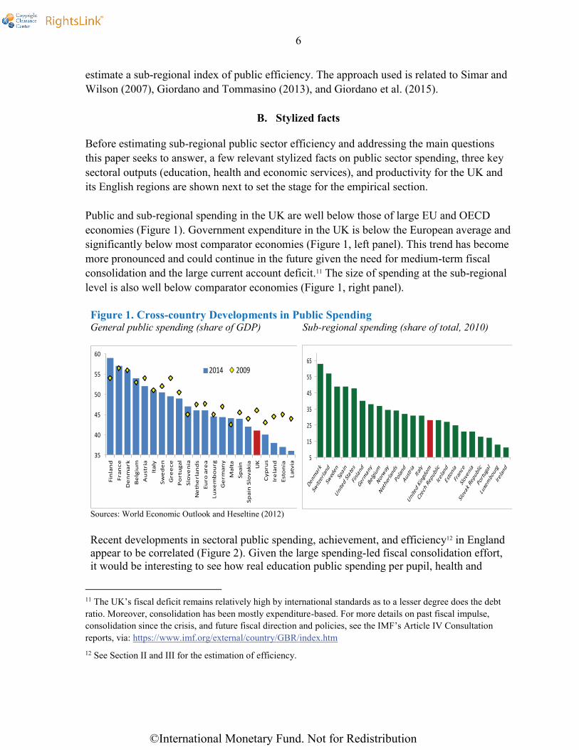
Public and sub-regional spending in the UK are well below those of large EU and OECD

economies (Figure 1). Government expenditure in the UK is below the European average and

significantly below most comparator economies (Figure 1, left panel). This trend has become

more pronounced and could continue in the future given the need for medium-term fiscal

consolidation and the large current account deficit.11 The size of spending at the sub-regional

level is also well below comparator economies (Figure 1, right panel).

Figure 1. Cross-country Developments in Public Spending General public spending (share of GDP) Sub-regional spending (share of total, 2010)

Sources: World Economic Outlook and Heseltine (2012)

Recent developments in sectoral public spending, achievement, and efficiency12 in England

appear to be correlated (Figure 2). Given the large spending-led fiscal consolidation effort,

it would be interesting to see how real education public spending per pupil, health and

11 The UK’s fiscal deficit remains relatively high by international standards as to a lesser degree does the debt

ratio. Moreover, consolidation has been mostly expenditure-based. For more details on past fiscal impulse,

consolidation since the crisis, and future fiscal direction and policies, see the IMF’s Article IV Consultation

reports, via: https://www.imf.org/external/country/GBR/index.htm

12 See Section II and III for the estimation of efficiency.

35

40

45

50

55

60

Fin

lan

d

Fra

nc

e

De

nm

ark

Be

lgiu

m

Au

stri

a

Ita

ly

Sw

ed

en

Gre

ec

e

Po

rtu

ga

l

Slo

ve

nia

Ne

the

rla

nd

s

Eu

ro a

rea

Lu

xe

mb

ou

rg

Ge

rma

ny

Ma

lta

Sp

ain

Sp

ain

Slo

va

kia

UK

Cy

pru

s

Ire

lan

d

Est

on

ia

La

tvia

2014 2009

5

15

25

35

45

55

65


https://www.imf.org/external/country/GBR/index.htm

7

economic service expenditure per head (inputs) changed between the pre- and post-crisis

periods, 2003–07 and 2010–14, respectively. It is also useful to see if there were any

changes in achievement (outputs) associated with these spending changes, for example

here in this paper, in high school education attainment of GCSE scores, life expectancy at

the age of 65 years, and the number of private enterprises created themselves.13 These

“inputs” and “outputs” have been widely used in the literature (e.g., Boyle, 2011; Giordano

and Tommasino, 2013; reports of the UK’s National Audit Office), and Section IV.B

examines a few alternative outputs.14 15 Caveats in the choice of these outputs should be

noted. First, cuts in primary education spending post-crisis would take some years to

influence GCSE scores and more intermediate results (such as Key Stage 2 scores) are not

examined due to data constraints at the sub-regional level. In addition, no distinction

between private and state schools or pupils has been made given data constraints. Having

said that, data from the Department of Education points to gradual improvement in

national Key Stage 2 scores and regional pupil-to-teacher ratios in both primary and

secondary education. Second, health spending not only aims to prolong life at birth or old

age, but also to improve the quality of life—for example, by relieving chronic pain or

addressing problems with mobility. Moreover, faster moving health outputs (e.g., hospital

waiting lists, numbers of surgeries or hospital and clinic visits) would be preferable—but

data limitations at the sub-regional level prevent such a choice. Also since life expectancy

is a slow moving variable, studying changes over an even longer time horizon may be

warranted—a task left for future research. Third, these and other quality adjustments, while

important, are not studied at the sub-regional level, and thus are left for future research.16

Still it could be argued that for private sector productivity, for example, what matters in the

end is the not the efficiency of public spending per se, but the actual quantity and quality

of public services that is being provided (even if there is some waste). For example, if the

decline in public spending on education was associated with a proportional decline in high

school achievement, that may be damaging to the UK’s productivity regardless of what

happened to public sector efficiency.

13 The number of active enterprises is considered to be a good proxy for the effectiveness of public spending on

economic affairs since enterprises take root and succeed in regions or sub-regions with adequate housing,

transport connectivity, job centres, and the like. And these enterprises in turn contribute to employment,

economic growth and productivity more broadly. Moreover, it should be noted that the structure of the English

economy has not altered dramatically since 2003 outside of Greater London. See Section IV.B for robustness

checks and alternative achievement (i.e. output) metrics.

14 HM Treasury’s “Public Expenditure by Country, Region and Function” Chapter 9, Table 9.15, which is the

source of the spending data in this paper (see data appendix), shows comparable spending data per head and

other summary statistics.

15 Recent National Audit Office and Department for Business Innovation and Skills reports show comparable

spending data and attainment proxies for health and education and other relevant summary statistics. In terms of

the choice of proxies of attainment, other studies have also used higher education or cross-country OECD PISA

scores for education (available at the national level) and life expectancy at birth or mortality rates for health.

Some alternatives are explored in Section IV.B of the paper, subject to data availability at the NUTS2 level.

16 The “quality” of these public services does vary at least at the level of NUTS1 region (see the Cavendish

Review (2013), the National Audit Office (2012) report, and various King’s Fund research papers and reports).


8

Scatter plots provide an intuitive first cut of the data at the 28 sub-regional and 8 regional

levels between 2003 to 2014. The plots suggest that the post-crisis changes in spending per

pupil and high school education attainment (proxied by the change in GSCE scores) are

strongly and negatively correlated (Figure 2, first left panel), as are the changes in spending

Figure 2. Sectoral Inputs and Outputs and Efficiency (Real £s per head or pupil, in percent)

Sources and notes: Author’s estimates based on official UK data at the NUTS1 level for inputs/spending and NUTS2

aggregated up to NUTS1 for outputs/achievement. Change refers to that between the average of the pre-crisis (2003-07)

and the post-crisis (2010-14), in percent. Spending is in real £s per head or pupil.


9

per pupil and estimated efficiency17 (Figure 2, first right panel), while the changes in health

spending per head and health output (proxied by the change in life expectancy at 65 years

of age) are positively correlated (Figure 2, second left panel), as are the changes in health

spending per head and estimated efficiency (Figure 2, second right panel). The picture is

less definitive for the changes in economic services (as proxied by the change in the

number of private enterprises), although some positive correlation is apparent between

inputs and outputs (Figure 2, third left panel) and negative between efficiency and inputs.

Underestimated regional transportation spending may be behind these results (see annex).

Figure 3. Post Crisis Change in Regional Public Spending vs. Achievements (in percent)

Sources and notes: Author’s estimates based on official UK data at the NUTS1 level for inputs/real spending and NUTS2

aggregated up to NUTS1 for outputs/achievement. Change between average pre (2003-07) and post (2010-14) crisis, in

percent. Spending is in real £s per head or pupil.

Another first cut at the data suggests that while the large spending-led consolidation meant

cuts across most spending categories in England, it was education spending per pupil that fell

most dramatically, but achievement (at least in terms of the outputs used in this paper) was

not adversely affected, rising instead across all sectors, including education (Figure 3 and

annex Tables A.1 and A.2). The following findings, aggregated to the regional NUTS1 level,

emerge:

Public health inputs or spending per head actually increased sharply across all English

regions without exception post-crisis despite the large fiscal consolidation (Figure 3,

yellow striped-bars),20 unlike that of education spending per pupil which declined sharply

17 See Section II and III for the estimation of efficiency.

20 The increases in real health spending could be overestimated if health sector deflators have not been adjusted

concomitantly with rising health care costs.

-30

-20

-10

0

10

20

30

40

50

60

North East North West Yorkshire & theHumber

East Midlands West Midlands East of England South East South West


10

(Figure 3, orange striped-bars), particularly in the North. These spending cuts in

education (which more than offset the health spending increases), were large with

considerable variation across regions. Changes in public spending on economic services

exhibit more sub-regional variation, with small cuts in some regions and small increases

in others (Figure 3, green striped-bars).

There was no proportional decline in outputs commensurate with the proportional decline

in spending, rather all outputs improved post crisis. In particular, life expectancy

increased marginally (health output);21 GCSE achievement improved sharply22 (education

output) most notably in the North and Midlands, and the number of enterprises expanded

a little (economic services output) across regions, most notably in the East of England

(Figure 3, yellow, orange and green solid-bars, respectively).23

These initial results suggest that despite large spending cuts, actual output (at least in terms

of “quantities” measured here) has not suffered—rather it seems that excess fat in public

spending has been trimmed.24 As mentioned, in the education sector in particular, Key Stage

2 results (tested at the end of primary school for pupils typically aged 11 years old) are

unavailable at the sub-regional level but data on teacher-to-pupil ratios and class size

(whether primary or high school) suggest gradual improvement post crisis.25 Clearly, factors

other than changes in public spending could be driving these improvements—for example,

technological improvements from computing, specific education and health sector reforms,26

and possibly incentives of sub-regional authorities to achieve greater “value for money” in

21 While this small improvement is an important achievement given that life expectancy is a slow moving

variable, the trend has been slowly upward in most OECD economies, including the UK.

22 The Department of Education points to GCSE score inflation, in part attributed to measurement issues rather

than a change in education output.

23 Despite these improvements, employers complain about skill deficiencies among the young and those with

relatively low education attainment. In addition, there is a high proportion of negative growth firms and room to

improve leadership and managerial capabilities (Heseltine 2012).

24 Afonso et al. (2007) estimated a measure of public sector of efficiency and showed that output efficiency

ranked 16th out of 23 OECD economies, suggestive of some waste in public expenditure.

25 It is difficult to include Key Stage 2 examination results not least because standards have been revised,

becoming more challenging. Nevertheless, the Department of Education reports improvements at this Stage (in

reading, writing and maths). Also since the early 2000s the number of pupils per qualified teacher has fallen.

26 Sector-specific reforms that could have contributed to the post-crisis increase in outputs are as follows. For

education, while reforms from the Thatcher to Blair governments (which aimed for greater diversity, flexibility

and choice, backed by school autonomy and central government accountability) produced better examination

results, they also resulted in greater variation (i.e., polarization of performance between the best and worst

schools) (Whitty 2000 and 2014). For health, private spending and productivity in the sector have fallen

recently (Lloyd 2015), possibly contributing to lower quality outputs despite a broad and complex set of

reforms since 1997—and yet many challenges remain (Boyle 2011).


11

the wake of fiscal decentralization, among others. And as mentioned, the “quality” of these

outputs has not been measured and may not have a clear sectoral variation. Moreover, the

long-term impact of the spending cuts may not be felt for years to come. Finally, it should be

noted that during the GFC employment (in education and health specifically and in the

overall economy more broadly) did not decline as sharply as in other OECD economies

affected by the GFC, with the national unemployment rate in the UK remaining well below

many of these economies. Hence, the cuts in spending do not appear to have affected at least

the “quantity” of teachers, despite their real wages seeing modest declines.27 This along with

lower pupil-to-teacher ratios (in primary and secondary) may well have contributed to some

of the improved outputs, along with the incentives induced from sharp cuts in spending per

pupil in the education sector, for example.

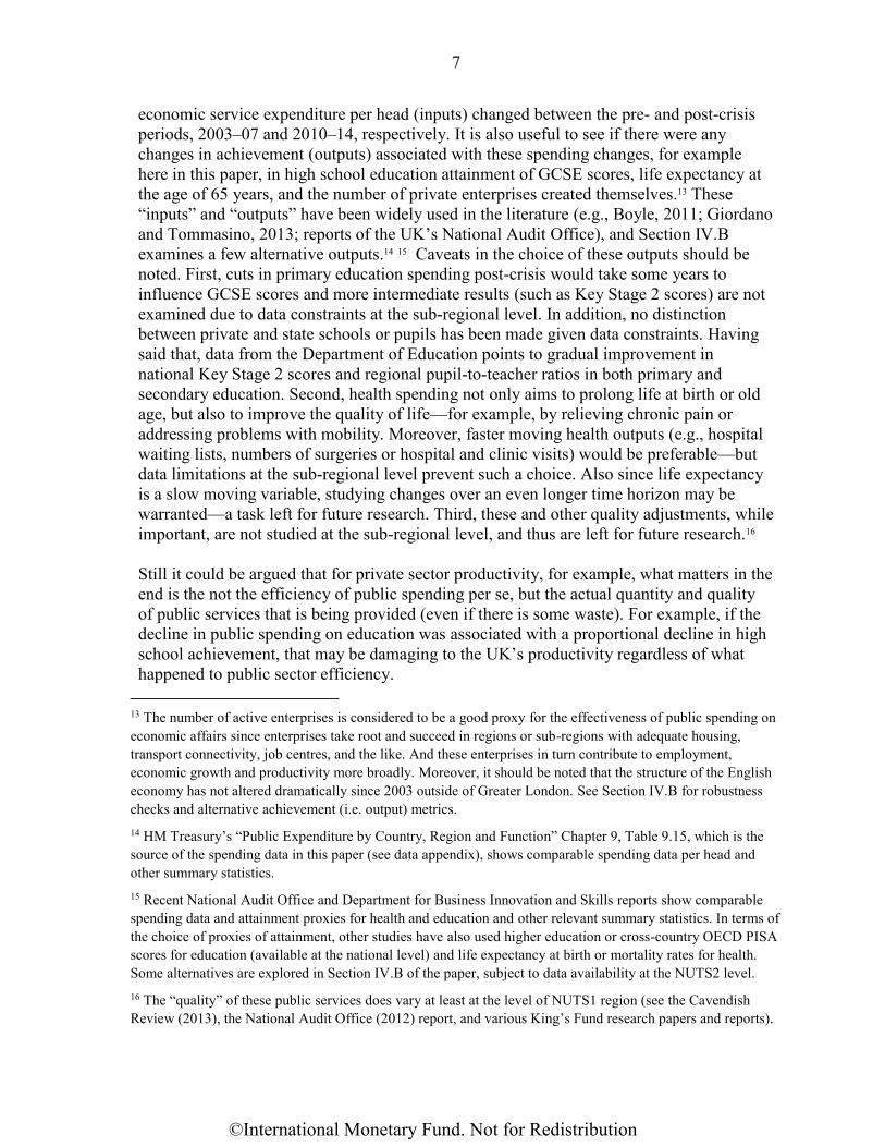
Figure 4. Cross-country Productivity

(average annual percent growth in output per hour)

After 2008, overall economic output productivity growth in the UK declined much more than

other advanced economies (Figure 4). Economic output productivity has been shown to be

associated with public sector productivity or efficiency—also a proxy for the quality of

governance (Giordano et al., 2015). Hence raising public sector productivity or efficiency

might help boost overall productivity in the UK, which has seen the average annual growth

of output per worker drop from almost 2 percent during 2000-08 to nearly zero during 2009-

27 Machin (2015) shows real wages to have declined nationally between 0.5 to 2.2 per annum between 2008-14

(explanations include a decoupling of wages and productivity growth; the decline of union membership and

thus collective wage bargaining; slack in labor market; among others). The Independent Newspaper reported

(on 10 January 2016) nominal teachers’ pay rises having been limited to around one percent for the past five

years, with schools finding it increasingly difficult to recruit qualified teachers. It also mentions that the

Department of Education sees “a record number of highly qualified teachers being attracted to the profession”.

Figure 1. Cross-country Productivity

0

1

2

3

0

1

2

3

UK USA Germany France

2000-08 2009-14

Productivity Slowdown in Selected Major Economies(Average annual percent growth in output per hour)

Sources: Haver Analytics and IMF staff calculations.


12

14 (Figure 4).28 As mentioned, the fact that the UK did not experience deep cuts in

employment may have contributed to the cyclical weak labor productivity growth, on the one

hand, and also in part supported the increase in outputs and efficiency in core sectors on the

other.

The rest of this paper is organized as follows. Section II lays out the evidence-based

empirical strategy, data and measurement issues and Section III reports the baseline results

on sub-regional public sector efficiency. Section IV presents robustness checks and Section

V draws conclusions and policy implications.

II. EMPIRICAL STRATEGY, DATA AND MEASUREMENT

Given the importance of public services to economic performance, this paper next combines

official public spending data and sectoral output measures from various government

departments to estimate an index of public productivity or efficiency at the sub-regional

English level. The methodology used follows Simar and Wilson (2007), with the approach

being related to Giordano and Tommasino (2013) and Giordano et al. (2015) who empirically

estimate an index of public service efficiency across Italian provinces. The latter studies do

not, however, differentiate between performance pre and post the GFC, for example, when

austerity led to large spending cuts. This is one of the novelties of this paper. In particular, it

constructs from scratch a sub-regional multi-sector public service (education, health and

economic services) database, aggregating (weighted from the town or local level upward) to

the NUTS2 sub-regional level, and then matching these with NUTS1 regional public

spending data. It then uses a regression framework to empirically estimate public sector

efficiency over two non-overlapping period averages: pre (2003–07) and post (2010–14) the

GFC, using annual data. This allows for an analysis of the evolution and variation of public

service delivery across England and its sub-regions (excluding London).29

A. Measuring public sector efficiency

Relation to the literature

Recent studies build on the microeconomic literature in measuring technical efficiency of a

unit of production, by establishing the difference between an actual and a potential unit of

output in relation to a unit of input—operational Pareto Optimality. Generalizing to all

“input-output pairs” allows the construction of an efficient production frontier that connects

or “envelopes” these combinations of input-output pairs, building on the idea of relative

efficiency (Farrell, 1957) using non-parametric linear programming—the so-called Data

28 See IMF 2016 and references therein for explanations and an analysis of this weak productivity growth.

29 Including London narrows variation across sub-regions vis-à-vis each other, but widens it vis-à-vis London.


13

Envelopment Analysis (DEA) developed by Charnes et al. (1978) and extended by Simar and

Wilson (2007).30 DEA allows multiple input-output pairs to be considered at the same time

without any assumption on data distribution. The relationship between spending (input) and

performance (output) is thus benchmarked despite its drivers not having been directly

observed.

Cross-country studies on public service efficiency or productivity using this approach include

Afonso et al. (2003 and 2007), Gupta et al. (2007), Verhoeven et al. (2007), and Grigoli

(2013). At the regional or local level, studies include Borge et al. (2008) for Norway, Revelli

(2010) for the UK, and Giordano and Tommasino (2013) for Italy. However, no study has yet

examined how public sector efficiency has changed sub-regionally post the GFC following a

large fiscal consolidation episode and across most spending categories or sectors.31 This is

one of the contributions of this paper.

Methodology

A sub-regional index of public sector efficiency is constructed using DEA regression analysis

based on total (central, regional, county, local) spending data on the three key public services

across the English regions: education, health, economic affairs (including transport and

housing).32 The regional spending data is complemented by sub-regional “control” variables,

e.g., changes in private spending on the examined public services, income per capita,

population density and its age-profile, and capital stocks, among others.

30 Non-parametric techniques, such as the Data Envelopment Analysis (DEA), typically do not control for the

diverse set of factors that influence outputs or outcomes—such as educational attainment, urbanization, private

spending on services, income, etc.—and thus collinearity arises. To control for the bias in the resultant

efficiency scores, the so-called “second stage” regression analysis (which simply refers to the inclusion of

control variables along with inputs on the left hand side of the regression equation (5) above) mitigates

measurement error and bias. See Ray (2004) for a comprehensive review of DEA. As a robustness, two separate

parametric stochastic frontier analysis (SFA) regressions are carried out in Section IV and thus complement the

DEA estimation.

31 Analysis of public sector performance has been carried out either at the UK national level following the 2005

Atkinson Review (e.g., ONS, 2017) or at the local spending level using only local spending, (e.g., Revelli

2010), which represents a small fraction of total spending—unlike this paper which covers total spending.

32 Other studies have estimated more aggregated measures of public sector efficiency across countries or

regions. For example, Charron (2013) estimated a quality of governance for all EU economies available at the

NUTS1 level. However, the measure suffers from some shortcomings (see Giordano et al. 2015). Aggregating

sub-regional public sector efficiency scores estimated in this paper to the regional level does suggests a

statistically significant (at the 5 percent level) and positive correlation with the Charron (2013) quality of

governance index for some periods. Afonso et al. (2007) also estimate a measure of public sector efficiency and

show that although the UK ranked seventh out of 23 OECD economies in terms of overall public sector

efficiency, output efficiency ranked 16th (out of 23).


14

Non-parametric treatment of the efficiency frontier does not assume a particular functional

form, but relies instead on the general regularity properties, such as monotonicity, convexity,

and homogeneity. The DEA is based on a linear programming algorithm,33 constructing an

efficiency frontier from the data in all “single decision units”—here being a sub-region or

county, such as the Greater Manchester Combined Authority. A DEA model can be sub-

divided into an input-oriented model (which minimizes inputs and controls while satisfying

at least a given level of output) or an output-oriented model (which maximizes outputs

without requiring more of any of the observed input or control values). The latter is chosen in

this paper, as these models are the most frequently used because the quantity and quality of

inputs (public spending and other controls defined here) are assumed to be fixed

exogenously, hence the sub-regional authorities cannot influence these, at least not in the

short-run.34

DEA models can also be subdivided in terms of returns to scale by adding weight constraints.

Constant returns to scale are chosen here as the baseline, as there is no conclusive evidence

to suggest that the production of public services (whether in health, education or economic

services) varies in technology across English regions or sub-regions outside Greater

London—particularly during the past four decades since the creation of the National Health

Service and the state school system, unlike firms. However, variable returns to scale

technologies (i.e., increasing or decreasing) were also estimated but do not suggest a material

change to the results.35 A specific sub-region is called efficient when the DEA score equals to

one and slack is zero. Inefficiency can be seen in terms of how much the inputs and control

variables must contract along a ray from the origin until it crosses the frontier (Ji and Lee,

2010).

Spending on the three categories of education, health, and economic affairs represents over

50 percent of total public spending over the past decade, with all three having been shown in

the literature to influence economic prospects over time (Afonso et al. 2003), and the

33 Limitations arise from the assumption of linearity in the production function. This is mitigated in part through

the use of parametric stochastic frontier analysis with a Cobb-Douglas technology in Section IV.C.

34 Input-oriented results are also estimated and shown in the appendix, yielding similar results (in terms of the

order or ranking of sub-regional performance).

35 The Attlee government centralized health spending in the 1940s and the Callaghan government did the same

for education in the mid-70s onward. Hence the delivery of these public services have become standardized,

broadly speaking, nation-wide since the post-war era, with limited variation by region or sub-region, and with

only about a quarter of this spending being local. Nevertheless, variable returns to scale technologies (i.e.,

increasing or decreasing) in the production of these services are also estimated (see appendix Table A.4) in case

there could be some regional variation, e.g., between the north and south of England, given differing population

densities, incomes, and other factors. No material change is evident (Table A.4).


15

remainder largely being spending on pensions and social protection.36 37 The assumption is

that this spending does not vary within each region, only across regions (Giordano and

Tommasino 2013, Giordano et al. 2015).38 By and large, all regions experienced public

spending cuts post crisis, with the exception of health—where spending per head rose across

regions with limited (NUTS1) regional variation (Figure 3 and Table A.1). On the other

hand, spending cuts in education (which offset the health spending increases), were large

with considerable variation across regions. For example, the North experienced cuts per pupil

between three to 8½ times more than the South (Figure 3 and Table A.1).

Performance outputs and other control variables vary within regions—in other words they are

available and have been collected from various government departments at the sub-regional

(NUTS2) level (see the data appendix). Two cross-sections are examined to compare the pre-

and post-crisis average performance (2003–07 vs. 2010–14) given data availability.39 This

allows for the coefficients to vary between the pre- and post-crisis periods, capturing the

dynamic changes. Outputs are those of the 28 English counties.40 41

B. Estimation

The DEA regression is estimated, for each of the two non-overlapping period averages, pre-

and post-crisis. The production process is constrained by the production set:

Ψ = {(𝑥, 𝑦) ∈ 𝑅+𝑁+𝑀|𝑥 𝑐𝑎𝑛 𝑝𝑟𝑜𝑑𝑢𝑐𝑒 𝑦} (1)

where 𝑥 represents a vector of 𝑁 inputs (public spending by sector and controls as specified

below for each sector) and 𝑦 the vector of 𝑀 outputs by sector (as shown in more detail

below). Three separate production processes are estimated for each sector. Each production

frontier is the boundary of Ψ. In the interior of the Ψ there are units that are technically

36 In this paper, all non-health and non-education spending is considered other than social protection (largely

pensions), defense and international chapters, to represent spending that influences “economic services”.

37 Arguably, social protection spending can also influence public sector efficiency, economic performance and

productivity—since caring for the elderly or disadvantaged can impact labor productivity if such labor is fully

or partly engaged in this type of care.

38 In practice targeting of under-privileged schools or hospitals in some sub-regions has taken place and may

result in variation within a sub-region. However, data is unavailable to test this at the sub-regional level.

39 The years 2008-09 are excluded owing to the global financial crisis and the consequent small fiscal stimulus.

Results are available upon request.

40 All English countries excluding the five parts of Greater London are shown—common practice in the

literature given London’s outlier and global city status.

41 See the Appendix for data specification and sources.


16

inefficient while technically efficient ones operate on the boundary of Ψ, i.e., the technology

frontier. If the production set is described by its sections, then the output requirement set is

described for all 𝑥 ∈ 𝑅+𝑁:

𝑌(𝑥) = {𝑦 ∈ 𝑅+𝑀|(𝑥, 𝑦) ∈ Ψ} (2)

The output-oriented efficiency boundary 𝜕𝑌(𝑥) is defined for a given 𝑥 ∈ 𝑅+𝑁 as:

𝜕𝑌(𝑥) = {𝑦|𝑦 ∈ 𝑌(𝑥), 𝜆𝑦 ∉ 𝑌(𝑥), ∀𝜆 > 1} (3)

and the output measure of efficiency for a production unit located at (𝑥, 𝑦) ∈ 𝑅+𝑁+𝑀(𝑥, 𝑦) is:

𝜆(𝑥, 𝑦) = 𝑠𝑢𝑝{𝜆|(𝑥, 𝜆𝑦) ∈ Ψ} (4)

Because the production function set Ψ is unobserved, in practice efficiency scores 𝜆(𝑥, 𝑦) are

obtained by DEA estimators, for example, for output orientation with constant returns to

scale, and the solution is found through the linear program:

�̂�𝐶𝑅𝑆(𝑥, 𝑦) = 𝑠𝑢𝑝{𝜆|𝑥, 𝜆𝑦 ≤ ∑ 𝛾𝑖𝑦𝑖𝑥 ≥ ∑ 𝛾𝑖𝑥𝑖 𝑓𝑜𝑟 (𝛾1, … 𝛾𝑛)𝑛𝑖=1

𝑛𝑖=1 } (5)

such that: 𝛾𝑖 ≥ 0, 𝑖 = 1, … , 𝑛

The three sectors are:

o Education. Input: Real public expenditure on education per pupil; Other inputs or

control variables: Private spending on education and education attainment by income

level per head; Output: High school (GCSE) achievement.44

o Health. Input: Real public expenditure on health per head; Other inputs or control

variables: Adjusted for population’s age structure (i.e., ratio of population over 65);45

and the prevalence of obesity. Output: Life expectancy at the age of 65 years.47

o Economy. Input: Real public expenditure on economic services, including transport and

housing, normalized by lagged population size; Other inputs or control variables:

Lagged stock of capital; Output: Number of active enterprises.48

44 Alternative outputs and control variables are examined for robustness in Section IV.B, as well as the issue of

lags in public spending.

45 This adjustment is made to reflect the fact that spending on the elderly could be larger for counties that have a

larger share of elderly in their total population.

47 This output is chosen since it is more ambitious (relative to life expectancy “at birth”) given the secular trend

in population aging. See Section IV.B for the use of life expectancy at birth.

48 See footnote 13 and Section IV.B for the use of labor productivity of these enterprises as an alternative output

for this sector.


17

III. BASELINE FINDINGS

This section examines the following questions: (i) Has sub-regional public sector efficiency

improved or weakened in England during the fiscal consolidation of 2010-14? (ii) What has

been the pattern across different sectors and sub-regions? (iii) Have sub-regions with lower

initial levels of efficiency experienced stronger gains, implying some catch up in efficiency

levels? (iv) Were deeper cuts in public spending associated with stronger efficiency gains?

(v) Has there been any relationship between changes in public sector efficiency and labor

productivity across sub-regions?

Sub-regional efficiency scores reassuringly show stability over the estimation sub-sample

periods (Table 1). The estimated efficiency scores, �̂�𝐶𝑅𝑆(𝑥, 𝑦), from the DEA regression

(equation 5) are presented for each sector and combined into a simple average—a weighted

average produces similar results (see Section IV.A). Higher values imply higher efficiency

and the score of one implies a county that was most efficient.49 Despite large public spending

cuts, overall efficiency improved post crisis (Table 1 and Figure 5). Efficiency improved

most notably in the education sector, which saw the deepest cuts, followed by health (which

instead saw spending increases). However, the efficiency of economic services deteriorated

slightly. In terms of sub-regions, at one end, Tees Valley and Durham (UKC1) improved its

efficiency post crisis, but at the other end, Devon, (UKK4), saw a deterioration (including but

not limited to the reduction in public spending). The lower quartile of efficiency, however,

remains a northern-county phenomenon. Determining whether the post crisis improvements

in efficiency scores are statistically significant is not straightforward, however. While

bootstrapping and Bayesian methods have been used to determine the statistical significance

of the DEA results, none of these methodologies can estimate, with a specified probability,

the confidence interval for the true efficiency scores.50

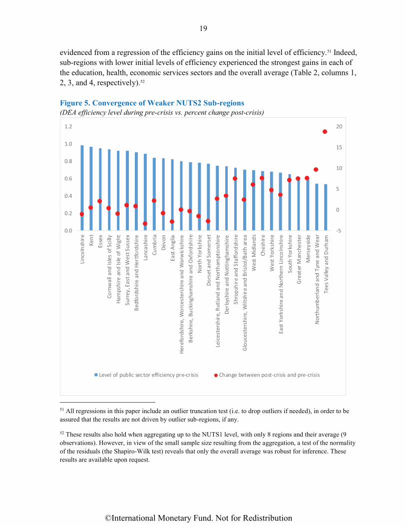
Sub-regions with the weakest pre-crisis levels in public sector efficiency converged the most

(Figure 5 and Table 2). Worse off sub-regions achieved the largest improvements, as

49 Results are reported for the output-oriented DEA. Alternative results for input-oriented DEA or variable

returns technologies suggest similar results (Appendix Tables A.3 and A.4, respectively).

50 Bootstrapping methodologies do not incorporate stochastic variations in each sub-region’s input-output

performance. Bayesian methods are based on variations in the frontier while ignoring variations within sub-

regional units. So, like bootstrapping, they can estimate the probability distribution for the efficiency of a fixed

set of inputs and outputs, but cannot estimate the probability distribution for the efficiency of the individual sub-

regions. Both bootstrapping and Bayesian estimation are based on one observation of each sub-region. I have

two observations per sub-region, and hence it is not possible to estimate variation without more observations.

Even for a cross-sectional analysis, one cannot determine whether a sub-region is efficient with a specified

degree of statistical significance nor construct confidence intervals within which the sub-region’s true efficiency

uptrends or downtrends are statistically significant or just random variations. For more details, see Barnum,

D.T., Gleason, J.M., Karlaftis, M.G., Schumock, G.T., Shields, K.L., Tandon, S. and Walton, S.M. (2011),

Estimating DEA Confidence Intervals with Statistical Panel Data Analysis. Journal of Applied Statistics, 39,

815-828.


1

8

Table 1. Public Sector Efficiency Scores Computed by Data Envelopment Analysis for English Counties 1

Combined

Efficiency

Index2

Combined

Efficiency

Index2

Country (NUTS2) Code

Tees Valley and Durham UKC1 0.77 0.68 0.16 0.54 0.98 0.72 0.21 0.64

Northumberland and Tyne and Wear UKC2 0.84 0.68 0.11 0.54 0.95 0.71 0.12 0.59

Merseyside UKD7 0.88 0.81 0.16 0.61 0.96 0.84 0.18 0.66

Greater Manchester UKD3 0.90 0.81 0.15 0.62 1.00 0.84 0.15 0.66

South Yorkshire UKE3 0.81 0.87 0.28 0.65 0.94 0.90 0.26 0.70

East Yorkshire and Northern Lincolnshire UKE1 0.88 0.88 0.27 0.67 0.93 0.90 0.26 0.70

West Yorkshire UKE4 0.89 0.87 0.28 0.68 0.95 0.90 0.30 0.71

Cheshire UKD6 0.88 0.86 0.33 0.69 0.97 0.90 0.36 0.74

West Midlands UKG3 0.89 0.89 0.31 0.70 1.00 0.90 0.33 0.74

Gloucestershire, Wiltshire and Bristol/Bath area UKK1 0.86 0.94 0.31 0.70 0.89 0.96 0.32 0.72

Shropshire and Staffordshire UKG2 0.86 0.90 0.43 0.73 0.94 0.91 0.51 0.78

Derbyshire and Nottinghamshire UKF1 0.88 0.94 0.41 0.74 0.95 0.95 0.41 0.77

Leicestershire, Rutland and Northamptonshire UKF2 0.86 0.96 0.44 0.75 0.89 0.96 0.46 0.77

Dorset and Somerset UKK2 0.93 0.97 0.42 0.78 0.87 0.98 0.41 0.75

North Yorkshire UKE2 1.00 0.93 0.43 0.79 0.98 0.96 0.38 0.77

Berkshire, Buckinghamshire and Oxfordshire UKJ1 1.00 1.00 0.38 0.79 0.99 0.99 0.38 0.79

Herefordshire, Worcestershire and Warwickshire UKG1 0.88 0.93 0.59 0.80 0.96 0.94 0.51 0.80

East Anglia UKH1 0.91 1.00 0.57 0.83 0.89 1.00 0.51 0.80

Devon UKK4 0.94 0.95 0.61 0.84 0.91 0.96 0.61 0.83

Cumbria UKD1 0.90 0.86 0.76 0.84 0.92 0.89 0.76 0.86

Lancashire UKD4 1.00 0.83 0.84 0.89 1.00 0.86 0.71 0.86

Bedfordshire and Hertfordshire UKH2 1.00 0.98 0.75 0.91 1.00 0.99 0.76 0.92

Surrey, East and West Sussex UKJ2 0.95 1.00 0.82 0.92 0.95 1.00 0.84 0.93

Hampshire and Isle of Wight UKJ3 0.94 0.99 0.84 0.92 0.92 0.99 0.84 0.91

Cornwall and Isles of Scilly UKK3 0.89 0.93 1.00 0.94 0.89 0.95 1.00 0.94

Essex UKH3 0.87 0.98 1.00 0.95 0.93 0.97 1.00 0.97

Kent UKJ4 0.94 0.96 1.00 0.97 0.95 0.97 1.00 0.97

Lincolnshire UKF3 1.00 0.96 1.00 0.99 0.96 0.97 1.00 0.98

England average (exl. London) 2 0.882 0.916 0.523 0.778 0.928 0.930 0.521 0.796

1 Constant returns to scale.2 Simple average.

Pre-crisis (2003-07)

Education Health EconomyEducation Health Economy

Post-crisis (2010-14)


19

evidenced from a regression of the efficiency gains on the initial level of efficiency.51 Indeed,

sub-regions with lower initial levels of efficiency experienced the strongest gains in each of

the education, health, economic services sectors and the overall average (Table 2, columns 1,

2, 3, and 4, respectively).52

Figure 5. Convergence of Weaker NUTS2 Sub-regions

(DEA efficiency level during pre-crisis vs. percent change post-crisis)

51 All regressions in this paper include an outlier truncation test (i.e. to drop outliers if needed), in order to be

assured that the results are not driven by outlier sub-regions, if any.

52 These results also hold when aggregating up to the NUTS1 level, with only 8 regions and their average (9

observations). However, in view of the small sample size resulting from the aggregation, a test of the normality

of the residuals (the Shapiro-Wilk test) reveals that only the overall average was robust for inference. These

results are available upon request.

-5

0

5

10

15

20

0.0

0.2

0.4

0.6

0.8

1.0

1.2

Lin

coln

shir

e

Ken

t

Esse

x

Co

rnw

all a

nd

Isl

es o

f Sci

lly

Ham

psh

ire

and

Isl

e o

f W

igh

t

Surr

ey, E

ast a

nd W

est S

usse

x

Bed

ford

shir

e an

d H

ertf

ord

shir

e

Lan

cash

ire

Cu

mb

ria

De

vo

n

East

An

glia

Her

efo

rdsh

ire,

Wo

rces

ters

hir

e an

d W

arw

icks

hir

e

Be

rksh

ire

, B

uck

ing

ha

msh

ire

an

d O

xfo

rdsh

ire

No

rth

Yo

rksh

ire

Do

rse

t a

nd

So

me

rse

t

Leic

este

rsh

ire,

Rut

land

and

Nor

tham

pto

nshi

re

Der

bysh

ire

and

Not

ting

ham

shir

e

Sh

rop

shir

e a

nd

Sta

ffo

rdsh

ire

Glo

uces

ters

hire

, Wilt

shir

e an

d B

rist

ol/B

ath

area

We

st M

idla

nd

s

Ch

esh

ire

We

st Y

ork

shir

e

East

Yor

kshi

re a

nd

No

rthe

rn L

inco

lnsh

ire

Sout

h Yo

rksh

ire

Gre

ater

Man

che

ste

r

Mer

seys

ide

No

rth

um

be

rlan

d a

nd

Tyn

e a

nd

We

ar

Tee

s V

alle

y a

nd

Du

rham

Level of public sector efficiency pre-crisis Change between post-crisis and pre-crisis


20

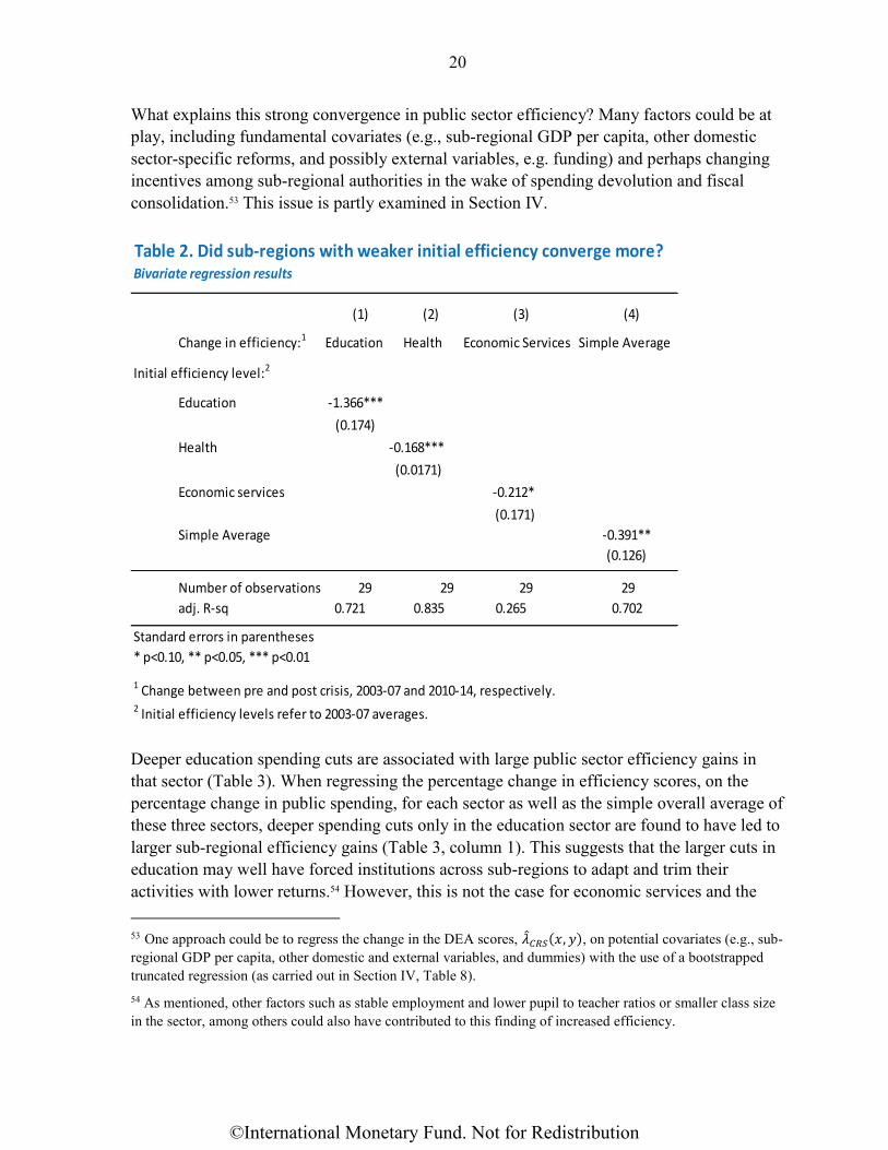
What explains this strong convergence in public sector efficiency? Many factors could be at

play, including fundamental covariates (e.g., sub-regional GDP per capita, other domestic

sector-specific reforms, and possibly external variables, e.g. funding) and perhaps changing

incentives among sub-regional authorities in the wake of spending devolution and fiscal

consolidation.53 This issue is partly examined in Section IV.

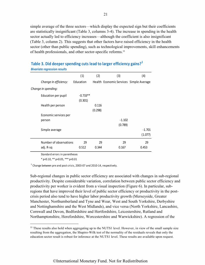
Deeper education spending cuts are associated with large public sector efficiency gains in

that sector (Table 3). When regressing the percentage change in efficiency scores, on the

percentage change in public spending, for each sector as well as the simple overall average of

these three sectors, deeper spending cuts only in the education sector are found to have led to

larger sub-regional efficiency gains (Table 3, column 1). This suggests that the larger cuts in

education may well have forced institutions across sub-regions to adapt and trim their

activities with lower returns.54 However, this is not the case for economic services and the

53 One approach could be to regress the change in the DEA scores, �̂�𝐶𝑅𝑆(𝑥, 𝑦), on potential covariates (e.g., sub-

regional GDP per capita, other domestic and external variables, and dummies) with the use of a bootstrapped

truncated regression (as carried out in Section IV, Table 8).

54 As mentioned, other factors such as stable employment and lower pupil to teacher ratios or smaller class size

in the sector, among others could also have contributed to this finding of increased efficiency.

Table 2. Did sub-regions with weaker initial efficiency converge more?Bivariate regression results

(1) (2) (3) (4)

Change in efficiency:1 Education Health Economic Services Simple Average

Initial efficiency level:2

Education -1.366***

(0.174)

Health -0.168***

(0.0171)

Economic services -0.212*

(0.171)

Simple Average -0.391**

(0.126)

Number of observations 29 29 29 29

adj. R-sq 0.721 0.835 0.265 0.702

Standard errors in parentheses

* p<0.10, ** p<0.05, *** p<0.01

1 Change between pre and post crisis, 2003-07 and 2010-14, respectively.2 Initial efficiency levels refer to 2003-07 averages.


21

simple average of the three sectors—which display the expected sign but their coefficients

are statistically insignificant (Table 3, columns 3-4). The increase in spending in the health

sector actually led to efficiency increases—although the coefficient is also insignificant

(Table 3, column 2). This suggests that other factors have raised efficiency in the health

sector (other than public spending), such as technological improvements, skill enhancements

of health professionals, and other sector-specific reforms.55

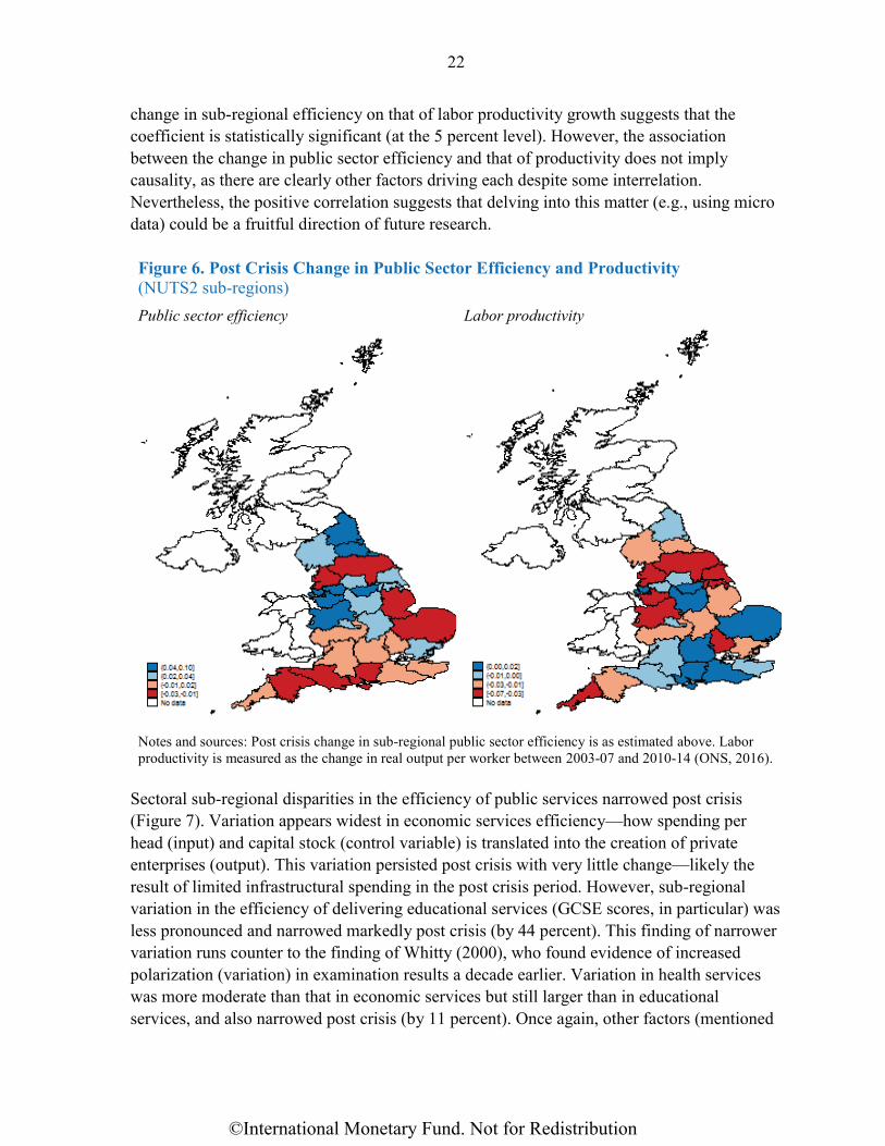
Sub-regional changes in public sector efficiency are associated with changes in sub-regional

productivity. Despite considerable variation, correlation between public sector efficiency and

productivity per worker is evident from a visual inspection (Figure 6). In particular, sub-

regions that have improved their level of public sector efficiency or productivity in the post-

crisis period also tend to have higher labor productivity growth (Merseyside, Greater

Manchester, Northumberland and Tyne and Wear, West and South Yorkshire, Derbyshire

and Nottinghamshire and the West Midlands), and vice versa (North Yorkshire, Lancashire,

Cornwall and Devon, Bedfordshire and Hertfordshire, Leicestershire, Rutland and

Northamptonshire, Herefordshire, Worcestershire and Warwickshire). A regression of the

55 These results also hold when aggregating up to the NUTS1 level. However, in view of the small sample size

resulting from the aggregation, the Shapiro-Wilk test of the normality of the residuals reveals that only the

education sector result is robust for inference at the NUTS1 level. These results are available upon request.

Table 3. Did deeper spending cuts lead to larger efficiency gains?1

Bivariate regression results

(1) (2) (3) (4)

Change in efficiency: Education Health Economic Services Simple Average

Change in spending:

Education per pupil -0.733**

(0.301)

Health per person 0.116

(0.298)

Economic services per

person -1.102

(0.789)

Simple average -1.701

(1.077)


adj. R-sq 0.512 0.344 0.167 0.453


* p<0.10, ** p<0.05, *** p<0.01

1 Change between pre and post crisis, 2003-07 and 2010-14, respectively.


22

change in sub-regional efficiency on that of labor productivity growth suggests that the

coefficient is statistically significant (at the 5 percent level). However, the association

between the change in public sector efficiency and that of productivity does not imply

causality, as there are clearly other factors driving each despite some interrelation.

Nevertheless, the positive correlation suggests that delving into this matter (e.g., using micro

data) could be a fruitful direction of future research.

Figure 6. Post Crisis Change in Public Sector Efficiency and Productivity

(NUTS2 sub-regions)

Public sector efficiency

Labor productivity

Notes and sources: Post crisis change in sub-regional public sector efficiency is as estimated above. Labor

productivity is measured as the change in real output per worker between 2003-07 and 2010-14 (ONS, 2016).

Sectoral sub-regional disparities in the efficiency of public services narrowed post crisis

(Figure 7). Variation appears widest in economic services efficiency—how spending per

head (input) and capital stock (control variable) is translated into the creation of private

enterprises (output). This variation persisted post crisis with very little change—likely the

result of limited infrastructural spending in the post crisis period. However, sub-regional

variation in the efficiency of delivering educational services (GCSE scores, in particular) was

less pronounced and narrowed markedly post crisis (by 44 percent). This finding of narrower

variation runs counter to the finding of Whitty (2000), who found evidence of increased

polarization (variation) in examination results a decade earlier. Variation in health services

was more moderate than that in economic services but still larger than in educational

services, and also narrowed post crisis (by 11 percent). Once again, other factors (mentioned


23

above) beyond the change in public spending could have contributed to the reported narrower

variation findings here. Section IV.C (Table 8) picks up the issue of the drivers of sub-

regional variation.

Figure 7. Disparities in Sub-Regional Public Sector Efficiency

IV. ROBUSTNESS CHECKS

Three sets of robustness checks are studied in this section. First, the estimated efficiency

scores are weighted by their corresponding sectoral shares of public spending. Second,

alternative outputs and control variables, among others, are considered, depending on data

availability. Third, as a complement to the DEA, a stochastic frontier analysis is undertaken

to address some reported endogeneity difficulties when measuring efficiency in the education

sector. This third check allows one to answer the following question: What are the drivers of

sub-regional efficiency variation post-crisis?

0

0.2

0.4

0.6

0.8

1

1.2

pre-

cris

is

post

-cri

sis

pre-

cris

is

post

-cri

sis

pre-

cris

is

post

-cri

sis

Avg. Max Min

Education Health Economy

Pre- and post-crisis refer to the 2003-07 and 2010-14 average, respectively.


24

A. Weighted average DEA scores

The DEA estimated efficiency

scores are weighted by their

corresponding sectoral shares of

public spending at the NUTS1

level, in case particular NUTS1

regions’ spending is concentrated

in one sector more than others, so

as not to under or overestimate

the combined average—instead

of the simple average of the three

sectors shown in Table 1. The

weights used are the average

shares of the sectoral spending

for the full sample (Table 4) and

result in a similar ranking of sub-

region efficiency (Table 5) with

all baseline results reported in

Section III holding.

B. Alternative inputs, outputs and control variables

Alternative or additional specifications of outputs and control variables are considered next,

depending on data availability, along with the issue of lags in public spending.

In the education sector, pupil to teacher ratios (or class size when unavailable) are used as an

additional control variable (given mentioned problems associated with GCSE score inflation

and other factors that could have contributed to increased education outputs post crisis),

while education spending is lagged for one year due to relatively strong contemporaneous

effects of public spending on achievement in the state school system, and in poorer sub-

regions in particular (Jackson et al. 2016). While previously mentioned caveats still hold,

including the problem of the absence of primary schooling outputs, the education sector

coefficients using higher order lags of public spending in Tables 6 and 7 were insignificant

albeit similar in magnitude and sign.56 The resultant DEA scores for the education sector do

not vary significantly from those shown in the baseline as a result of these robustness checks

(Table 5).

56 These results are available upon request.

Table 4. Average weights of main spending categories 1

( £ '000)

NUTS1 Economic services Health Education Total

UKC 4,225 4,898 3,511 12,635

0.33 0.39 0.28

UKD 11,462 12,799 9,202 33,463

0.34 0.38 0.28

UKE 7,567 8,881 6,876 23,324

0.32 0.38 0.29

UKF 5,903 6,871 5,583 18,357

0.32 0.37 0.30

UKG 7,547 9,422 7,261 24,230

0.31 0.39 0.30

UKH 7,297 8,715 6,841 22,853

0.32 0.38 0.30

UKJ 10,562 13,104 9,994 33,661

0.31 0.39 0.30

UKK 6,837 8,180 6,143 21,159

0.32 0.39 0.29

1 Average weights during 2003-14 of NUTS1 spending for England excluding London.


2

5

Table 5. Robustness--Weighted Public Sector Efficiency Scores Computed by Data Envelopment Analysis 1

Combined

Efficiency

Index2

Combined

Efficiency

Index2





Merseyside UKD7 0.24 0.31 0.06 0.60 0.26 0.32 0.06 0.65



Cheshire UKD6 0.24 0.33 0.11 0.68 0.27 0.34 0.12 0.73











East Anglia UKH1 0.27 0.38 0.18 0.83 0.27 0.38 0.16 0.81

Cumbria UKD1 0.25 0.33 0.26 0.84 0.25 0.34 0.26 0.86

Devon UKK4 0.27 0.37 0.20 0.84 0.27 0.37 0.20 0.83

Lancashire UKD4 0.28 0.32 0.29 0.88 0.28 0.33 0.24 0.85





Essex UKH3 0.26 0.37 0.32 0.95 0.28 0.37 0.32 0.97

Kent UKJ4 0.28 0.37 0.31 0.97 0.28 0.38 0.31 0.97


England average (exl. London) 2 0.264 0.348 0.169 0.780 0.276 0.354 0.168 0.797

1 Constant returns to scale.2 Weighted average.


Pre-crisis (2003-07) Post-crisis (2010-14)



26

For the health sector, instead of (the tougher) life expectancy at the age of 65 years, life

expectancy at birth (HALE) is the main output, health spending is lagged two years to reflect

some non-contemporaneous dynamics, and two additional control variables (or inputs) are

added: private spending on health from household surveys, and the smoking status at the time

of birth delivery.57 58 Despite these new variables, the output still suffers from the caveats

noted earlier and thus the results should still be interpreted with some caution. The resultant

DEA efficiency scores do not alter in terms of the sub-regional ranking for the health sector

nor do the changes post crisis (Table 5).

As an alternative to the number of enterprises created, labor productivity is used for the

output for public economic service spending,59 with spending itself lagged two years. Here

there were some changes in the ranking order of sub-regions, unlike other checks, however

the post crisis changes remain in the same order or magnitude as those reported in the

baseline (Table 5).

Using these alternative inputs, outputs and controls presented in this section, the baseline

result that sub-regions with the weakest levels of public sector efficiency converged the most

(when re-estimating the regression of the efficiency gains post crisis on the initial level pre

crisis, for each sector as well as the weighted overall average of the three sectors) still holds,

with each co-efficient displaying the same sign, similar magnitudes, and with slightly more

statistical significance and larger R-square (Table 6).60

Turning to the robustness of the baseline results shown earlier in terms of whether deeper

spending cuts have led to larger efficiency gains (when re-estimating the regression of the

percentage change in efficiency on the percentage change in public spending, for each sector

as well as the weighted overall average of these three sectors), the results suggest that not

only are the coefficients slightly larger, but now they also gain in statistical significance and

have larger R-square (Table 7).61 Despite these results, the problem of the endogeneity of

57 Using household income from survey data as an alternative did not alter the results materially.

58 As mentioned, although measuring the impact of health spending by looking at life expectancy misses the fact

that much of this spending seeks to improve the quality and not the duration of life, life expectancy is often used

as the main output proxy in the literature. While spending that relieves chronic pain or addresses mobility

problems, which may not prolong life, is not wasteful it is still unlikely to vary significantly across sub-regions.

Faster moving health outputs (surgeries performed or waiting lists) are not readily available sub-regionally.

59 See the discussion in footnote 13.

60 These results also hold when aggregating up to the small sample at the NUTS1 level, and are available upon

request, but not all residuals pass the normalcy test. Hence the results generalized to the NUTS1 level should be

interpreted with caution.

61 These results also hold when aggregating up to the small sample at the NUTS1 level and are available from

the author, but not all residuals pass the normalcy test.


27

Table 6. Robustness: Did sub-regions with weaker initial efficiency converge more?Bivariate regression results

(1) (2) (3) (4)

Change in efficiency:1 Education2 Health3 Economic Services4 Weighted Average

Initial efficiency level:1

Education2 -1.343***

(0.121)

Health3 -0.211**

(0.0141)

Economic services4 -1.143**

(0.026)

Weighted Average -0.677**

(0.117)


adj. R-sq 0.710 0.913 0.353 0.790


* p<0.10, ** p<0.05, *** p<0.01

1 Change between weighted efficiency index pre and post crisis, 2003-07 and 2010-14, respectively. Initial efficiency

levels refer to 2003-07 averages.

2 Education spending is lagged one year (two lags were insignificant), and NUTS2 teacher-pupil ratios are included as

a control variable. On the latter, data is only available since 2006.

3 Private health spending is added as a control from household surveys, as is a mother's smoking status

at time of delivery (data is only available since 2006), and life expectancy at birth (HALE) is the output.

4 Economic service spending is lagged two years (one year lags were insignificant) and the output here is

labor producivity.

Table 7. Robustness: Did deeper spending cuts lead to larger efficiency gains?1

Bivariate regression results

(1) (2) (3) (4)

Change in efficiency:1 Education2 Health3 Economic Services4 Weighted Average

Change in spending:

Education (per pupil)2 -0.728***

(0.301)

Health (per person)3 0.166***

(0.268)

Economic services (per

person)4 -1.301*

(0.801)

Weighted Average -1.789**

(1.078)


adj. R-sq 0.548 0.484 0.378 0.484


* p<0.10, ** p<0.05, *** p<0.01

1 Change between weighted efficiency index pre and post crisis, 2003-07 and 2010-14, respectively.

2 Education spending is lagged one year (two lags were insignificant), and NUTS2 teacher-pupil ratios are included

as a control variable. On the latter, data is only available since 2006.

3 Private health spending is added as a control from household surveys, as is a mother's smoking status at

time of delivery (data is only available since 2006), and life expectancy at birth (HALE) is the output.

4 Economic service spending is lagged two years (one year lags were insignificant) and the output here is labor

producivity.


28

public spending remains. Hence the next section attempts to address the issue through a two-

stage regression framework.

C. Stochastic frontier analysis

First-stage analysis

One of the limitations of the DEA efficiency estimation is its inability to fully control for

heterogeneity, for example, in terms of differences in levels of development or income

(Green, 2004; Grigoli, 2014). While control variables were introduced to address sub-

regional differences across England in the baseline DEA estimation (Section II and III) for

robustness, a parametric stochastic frontier analysis is examined next.

Parametric techniques, including stochastic frontier analysis (SFA), are essentially

econometric models requiring assumptions regarding the functional form of the production

frontier. Advantages of the parametric approach relative to the non-parametric ones (as in the

DEA) include controlling for a larger number of variables (that can influence each public

sector output, in this case) and more limited sensitivity to outliers. Both are particularly

relevant for cross-country studies, e.g., when studying differences among a heterogeneous

group—such as for developing versus advanced economies. But they also are relevant to

“within country” analyses—for example, here the issue of outliers was one of the reasons

behind excluding Greater London in the analysis.

The SFA approach is similar to the DEA in that a technological frontier envelops all input-

output pairs. In addition, from the statistical point of view, the regression model is

characterized by a composite error term in which the idiosyncratic (normally distributed)

disturbance capturing measurement error is included together with a one-sided disturbance

which represents inefficiency.

Two SFA cross-sections are estimated using a Cobb-Douglas production function for each

sector and for each of the pre- and post-crisis sub-sample averages, which are identical to

those in the baseline DEA efficiency estimation. The cross-sections are estimated by

maximum likelihood, with the difference from the DEA being that the estimation is carried

out in two separate steps. The first step is a regression of each sector’s outputs on its lagged

inputs to estimate SFA efficiency scores.62 The inputs and outputs are precisely those

introduced in this section—i.e., the “alternative inputs and outputs” described on pages 23-

25. As can be seen from the results of the SFA cross-sectional estimation (Figure 8),63 the

62 For a more complete description and examples from the applied economics literature see, for example,

Greene 2004 and 2008, Verhoeven et al. 2007, Fried et al. 2008, Belotti et al. 2012, Grigoli et al. 2013, and

Grigoli 2014. See also Belotti et al. (2012) for SFA cross-sectional regression formulations.

63 These results can be compared to those of the DEA estimation shown in Figure 5 and Table 5.


29

sub-regional efficiency scores are smaller in size but their ranking and magnitude of change

post crisis (or convergence) are highly and significantly correlated to those estimated in the

baseline DEA (whether for the simple or weighted average scores), despite the fact that no

control variables have been included in the SFA estimation yet—although now there is more

variation in the sub-regional scores (i.e., distance from the frontier).

Figure 8. Robustness: Convergence of Weaker NUTS2 Sub-regions

(Estimated SFA weighted-average efficiency pre-crisis levels vs. percent change post crisis)

Second-stage analysis

The second step estimates the determinants or covariates of sub-regional public sector

spending efficiency in the three sectors of education, health and economic services and the

weighted overall sectoral average. This separate second step partly addresses the problem of

public spending endogeneity, particularly if using lags in public spending among other

instruments. The SFA efficiency scores can be thought of as a rescaled measure of how much

GSCE achievement, for example, a sub-region can achieve at the spending levels pre- or

-10

-5

0

5

10

15

20

0.0

0.1

0.2

0.3

0.4

0.5

0.6

0.7

0.8

0.9

1.0

Lin

coln

shir

e

Ken

t

Esse

x

Co

rnw

all a

nd

Isl

es o

f Sci

lly

Ham

pshi

re a

nd

Isle

of

Wig

ht

Surr

ey, E

ast a

nd W

est S

usse

x

Be

dfo

rdsh

ire

an

d H

ert

ford

shir

e

Lanc

ashi

re

Cum

bri

a

Dev

on

Ea

st A

ng

lia

Her

efo

rdsh

ire,

Wo

rces

ters

hir

e an

d W

arw

icks

hir

e

Ber

kshi

re, B

uck

ingh

amsh

ire

and

Oxf

ord

shir

e

Nor

th Y

orks

hire

Do

rset

an

d S

om

erse

t

Leic

este

rsh

ire,

Rut

land

and

Nor

tham

pto

nshi

re

De

rbys

hir

e a

nd

No

ttin

gh

am

shir

e

Shro

psh

ire

and

Sta

ffo

rdsh

ire

Glo

uces

ters

hire

, Wilt

shir

e an

d B

rist

ol/B

ath

area

Wes

t M

idla

nds

Ch

esh

ire

Wes

t Yo

rksh

ire

East

Yor

kshi

re a

nd

No

rthe

rn L

inco

lnsh

ire

Sou

th Y

ork

shir

e

Gre

ater

Man

ches

ter

Me

rse

ysi

de

No

rth

um

ber

lan

d a

nd

Tyn

e an

d W

ear

Te

es

Va

lley

an

d D

urh

am

Level of public sector efficiency pre-crisis Change between post-crisis and pre-crisis


30

post-crisis if it were as efficient as the most efficient sub-region in England during the same

periods.

A multivariate truncated regression with fixed effects is run to identify the factors that

account for the sub-regional variation in the efficiency scores given that the SFA efficiency

scores are bounded (between zero and one).64 For this truncated regression, all estimated SFA

scores during the pre- and post-crisis periods (28 sub-regions and their average x 2-period

averages, and hence 58 observations) are included on the left hand side, and all control

64 For more details on the estimation approach and specifications used in the literature, see Green (2004) for

health, and Grigoli (2014) for education.

Table 8. Robustness: Determinants of sub-regional (NUTS2) spending efficiency scores? 1

Multivariate truncated regression results

(1) (2) (3) (4)

Education Health Economic Services Weighted Average

Regressors

Income per capita 0.012*** 0.000 0.001 0.000

(0.001) (0.001) (0.001) (0.001)

Private spending on education 1.132***

(0.206)

Private spending on health 0.020

(0.266)

Education attainment 2.412*** 3.101*** 3.001*** 3.000***

(0.214) (0.311) (0.300) (0.311)

Teacher to pupil ratio 0.024**

(0.002)

Population density 1.362* 1.561*** 1.542*** 1.442***

(0.171) (0.180) (0.181) (0.172)

Smoking status 0.000

(0.001)

Prevelance of obesity 0.000

(0.001)

Capital stock -0.001 -0.001*

(0.001) (0.001)

Active enterprises 0.012***

(0.022)


Fixed effects yes yes yes yes


* p<0.10, ** p<0.05, *** p<0.01

1 Two sets of efficiency scores per sub-region for each of the pre- and post-crisis periods and each regressor.

(Dependent variable: SFA efficiency scores)


31

variables along with a fixed effect per sub-region per period average are on the right hand

side. The results suggest (Table 8):

Income per capita. This captures the effect of disposable income on high-school

education achievement (GCSEs) and life expectancy at birth. The coefficient is positive

but small as expected, and is statistically significant only in the case of education. The

insignificant coefficient on health suggests that the NHS has contributed to improved

sub-regional health outputs regardless of private disposable incomes.

Private spending on education or health. This captures the effect of households’ ability

to complement public spending in achieving better high-school education and health

outputs. The coefficient is positive and large in the case of education but small and

statistically insignificant in the case of health. The former suggests that private spending

on students during the GCSE year (and one-year prior) is important and contributed

significantly to sub-regional variation in attainment. The latter suggests that while private

spending on health displays the right sign, it is insignificant in terms of explaining sub-

regional variation.

Education attainment by income level. Higher education attainment of parents or the

sub-regional population is likely to imply better GSCE achievement of their children and

similarly better health and economic service outputs. All coefficients are positive, large

and statistically significant, suggesting that education attainment does indeed explain a

large fraction of the sub-regional variation in efficiency scores.

Pupil-to-teacher ratio. In many OECD countries, a lower number of pupils per teacher

(or smaller class-size) is commonly associated with more efficient public spending on

high school education (Grigoli, 2014; Jackson, 2016). The coefficient is indeed positive

for secondary education albeit small and is statistically significant.

Population density. The quantity and quality of public services provided in education,

health, and economic affairs is usually easier to carry out in areas that are urban or more

densely populated since commuting distances are shorter and the diffusion or transfer of

knowledge and innovation is faster and competition brisker than in rural areas. As

expected the coefficients are positive, large and statistically significant for all sectors

implying that population density (a proxy for “connectivity” perhaps) is also an important

factor explaining the variation in spending efficiency across all sectors.

Smoking status at time of delivery. For the health sector alone, the smoking status of

the family at the time of the delivery of a birth could be associated with life expectancy at

that time. The coefficient is positive but small and insignificant, implying that smoking is

not an important factor explaining the variation in sub-regional public health spending

efficiency.


32

Prevalence of obesity. Once again, for the health sector alone, the prevalence of obesity

in mothers at the time of the delivery of a birth could be associated with the life

expectancy of the child born at that time. The coefficient is positive but small and

insignificant, implying that obesity has not been an important factor explaining the

variation in public health spending efficiency.

Capital stock. For economic services and the weighted average alone, larger capital

stocks could be associated with higher economic service efficiency scores since higher

capital output ratios augment and influence labor productivity as they contribute not only

to easing transportation and housing bottlenecks, but also bring in more jobs and

opportunities that would increase efficiency diffusion. However, the coefficient does not

display the expected sign, is small and only statistically significant in the case of the

weighted average. This could reflect measurement error in the input, which is likely to be

underestimated (see the data appendix).

Number of active enterprises. For economic services alone, more abundant firms could

be associated with higher public economic service efficiency scores; since the more

abundant the firms, the more experienced and sophisticated are the public service

providers in terms of the delivery of auxiliary business services offered. As expected, the

coefficient is positive, large and statistically significant, suggesting that the creation of

firms is an important determinant of sub-regional efficiency variation.

Overall, it appears that the most important determinant of sub-regional variation in public

sector service productivity or efficiency since 2003 is education attainment, followed by

population density (a proxy for urbanization or connectivity), and then private spending and

class size on education.

V. CONCLUSIONS AND POLICY IMPLICATIONS

How public sector efficiency or productivity changes during large fiscal consolidation

episodes is relevant since efficiency gains can help limit to some extent, along with other

secular trends, the adverse impact of spending cuts on outputs. Yet, there is little evidence on

how large “exogenous” fiscal consolidation episodes affect sub-regional public sector

efficiency and its variation. Despite data limitations at the sub-regional level, and therefore

several caveats to the paper’s findings, it offers a first stab at filling the gap in terms of what

has happened to sub-regional multi-sector public sector productivity post crisis. Its findings

could help inform multi-sector spending reforms in the wake of fiscal spending devolution in

England at this sub-regional (county or Combined Authority) level. The paper first found that

the actual “quantity” of public services provided post crisis broadly has not declined with the

proportional decline in education spending per pupil or spending in economic services, for

example. Moreover, health spending per head and its associated outputs have increased post

crisis.


33

While these results are encouraging, other factors could also be at play—such as

technological improvements, sector reforms, stable employment and incentives of sub-

regional authorities in the wake of fiscal devolution. In addition, the choice of outputs in both

the education and health sectors does suffer from some shortcomings—therefore making data

available on more complete (e.g., Key Stage 2 examination results) and faster moving (e.g.,

hospital waiting lists) outputs at the sub-regional level would aid further study. In addition,

despite these assuring and somewhat unexpected findings, employers have complained about

skill deficiencies among the young and those with relatively low education attainment. There

is also a high proportion of negative growth firms and room to improve managerial

capabilities in the economy (Heseltine 2012). Changes to the “quality of outputs” has also

not been measured. Finally, the long-term impact of some of the spending cuts may not be

felt for years to come, especially concerning health outputs (as this is a slow moving

variable) and the impact of cuts in primary education on high school achievement and

education attainment in England more broadly. Further analysis using micro data at the sub-

regional level, for example, could provide a fruitful avenue of future research and

complement the research undertaken in this paper.

Nevertheless, the paper sought to answer the central question of how much has public sector

service efficiency or productivity in sub-regional England and its variation changed since the

crisis following the large fiscal consolidation in an evidence-based (empirical) setting. After

constructing a sub-regional database that combines official public spending variables

matched with several leading multi-sectoral output measures used in the literature from

various government departments, an index of public efficiency at the sub-regional English

level is estimated.

Through a regression framework, the main empirical findings are: (i) despite large public

spending cuts, most notably in the education sector, overall efficiency improved post crisis,

with larger cuts yielding the highest efficiency improvements across sub-regions most

notably in the education sector, although the lower quartile remains a northern-county

phenomenon; (ii) notwithstanding lower initial efficiency levels, these northern counties

made the largest efficiency gains post crisis, thus contributing to a narrowing in regional

disparities across England; (iii) and while sectoral disparities in the efficiency of delivering

public services in economic affairs were widest and remained broadly unchanged post-crisis,

those for education (following spending cuts, among other factors) and health (following

spending increases, among other factors) have narrowed markedly.

These results could help inform policy makers when designing fiscal spending reforms,

including decentralization, across the English sub-regions. In particular, spending powers to

those sub-regions that delivered the largest improvements in efficiency could be devolved

first, and if the improvements persist, consideration could be given to granting revenue


34

generation powers next, for example. However, for those which saw a deterioration,

benchmarking as an incentive to improve future performance could be warranted.

Robustness checks revealed that the drivers behind sub-regional variation in public sector

efficiency levels since 2003 were fundamental factors such as education attainment of

households, population density, private spending on high school education and class size.

These could be a sign that reforms to increase sub-regional connectivity (and reduce the costs

of transportation) while increasing education attainment and reforms in some sub-regions are

worthwhile (for many sound economic reasons, not least) because they would help narrow

sub-regional disparities in public sector productivity further.

Finally, the paper found that post-crisis sub-regional changes in public sector efficiency are

associated with changes in post-crisis sub-regional labor productivity. However, given the

finding that public sector efficiency has improved, this suggests that either there are lags

between the two variables, with productivity possibly improving with a delay post

improvement in public sector efficiency, and that there are other factors beyond the change in

public sector efficiency driving the UK’s weak “productivity puzzle”. Exploring these factors

and continuing to delve more deeply into the UK’s productivity puzzle at the sub-regional

level would be an important avenue for future research.


35

References

Afonso, A., V. Tanzi, L. Schuknecht, 2003. “Public Sector Efficiency: An International

Comparison, ECB Working Paper No. 242.

Afonso, A., V. Tanzi, L. Schuknecht and N. Veldhuis, 2007. “Public Sector Efficiency: An

International Comparison, Fraser Alert, The Fraser Institute.

Atkinson, T., 2005. “Atkinson Review: Final Report—Measurement of Government Outputs

and Productivity for the National Accounts”, Palgrave MacMillan.

Belotti, F., S. Daidone, and G. Ilardi, 2012. “Stochastic frontier analysis using Stata,” Centre

for Economic and International Studies, Research Paper Series, Vol. 10, Issue 12,

No.251 (sept. 2012).

Borge, L-E., T. Falch, P. Tovmo, 2008. “Public Sector Efficiency: The Roles of the Political

and Budgetary Institutions, fiscal capacity, and Democratic Participation”, Public

Choice (2008) 136: 475-495.

Boyle, S., 2011. “Health Systems in Transition”, United Kingdom (England).

Charron, N., 2012. “From Aland to Ankara: European Quality of Government Index”,

University of Gothenburg Working Papers 2013:11

Evans, P., and J.E. Rauch, 1999. “Bureaucracy and Growth: A cross-National Analysis of the

Effects of “Weberian” State Structures on Economic Growth,” American Sociological

Review, Vol. 64(5), pp. 748-765.

Farrell, M.J., 1957. "The Measurement of Productive Efficiency," Journal of the Royal

Statistical Society vol. 120, pp. 253–281.

Fried, H., K. Lovell, and S. Schmidt, 2008. “The Measurement of Productive Efficiency and

Productivity growth (Oxford: Oxford University press).

Giordano, R., and P. Tommasino, 2013. "Public-Sector Efficiency and Political Culture,"

FinanzArchiv: Public Finance Analysis, Mohr Siebeck, Tübingen, vol. 69(3), pages

289-316, September.

Giordano, R., S. Landau, P. Tommasino, P. Topalova, 2015. “Does Public Spending

Inefficiency Constrain Firm Productivity: Evidence from Italian Provinces”. IMF

Working Paper 15/168.

Greene, W., 2004. “Distinguishing between Heterogeneity and Inefficiency: Stochastic

Frontier Analysis of the World Health Organization’s Panel Data on Health Care

Systems,” Health Economics, Vol. 13, pp. 959-80.

Green, W., 2008. The Measurement of Efficiency, chap. The Economic Approach to

Efficiency Analysis. Oxford University Press.

Grigoli, F. and J. Kapsoli, 2013. “Waste Note, Want Not: The Efficiency of Health

Expenditure in Emerging and Developing Economies.” IMF Working paper 13/187.

Grigoli, F., 2014. “A Hybrid Approach to Estimating the Efficiency of Public Spending on

Education in emerging and developing Economies.” IMF Working paper 14/19.


36

Heseltine, M., 2012. “No Stone Unturned—In Pursuit of Growth.”

Hughes, A., 2008. “Entrepreneurship and Innovation Policy: Retrospect and Prospect.”

Political Quarterly 79, 2008.

International Monetary Fund, 2016. The UK Article IV Consultation and Selected Issues

Paper, 2016.

Jackson, C. K., R. C. Johnson, and C. Persico, 2016. “The Effects of School Spending on

Educational and Economic Outcomes: Evidence from School Finance Reforms”,

Quarterly Journal of Economics (2016), 157-218.

Ji, Y-b, and C. Lee, 2010. “Data Envelopment Analysis”, The Stata Journal (2010) 10,

Number 2, pp. 267-280.

Kibblewhite, A., 2011. “Role of Public Sector Performance in Economic Growth,” Speech

delivered by Mr. Kibblewhite, Deputy Chief Executive, The Treasury, at the Institute

of Policy Studies, Wellington, 1 April 2011

Lloyd, T., 2015. “Historical trends in the UK: Funding Overview”, The Health Foundation.

Machin, S., 2015. “Real Wage Trends”, Understanding the Great Recession: From Micro to

Macro Conference, Bank of England, Sept. 23-24 2015.

Oats, W., 1972. Fiscal Federalism (New York: Harcourt Brace Jovanovich).

Office of National Statistics, 2017. “Public service productivity estimates: total public

service, UK:2104.” Office of National Statistics.

Phillips, D., 2015. “Local Government and the Nations: A Devolution Revolution?” Institute

of Fiscal Studies.

Ray, S., 2004. “Data Envelopment Analysis: Theory and Techniques for Economies and

Operations Research (Cambridge: Cambridge University Press).

Revelli, F., 2010. “Spend More, Get More? Any Inquiry into English Local Government

Performance”. Oxford Economic Papers 62(2010), 185-207

Simar, L., and P. W. Wilson, 2007. “Estimation and Inference in Two-stage, Non-parametric

Models of Production Processes. Journal of Econometrics, 136-64.

Travers, T., 2015. “A Hyper-Centralized Anomaly: why the UK Must Embrace Tax

Devolution”, in Tax for Our Times: How the Left Can Reinvent Taxation, edited by

D-R Smith, Fabian Ideas 640.

Verhoeven, M., V. Gunnarsson, and S. Carcillo, 2007. “Education and Health in G7

Countries: Achieving Better Outcomes with Less Spending,” IMF Working paper

07/263.

Whitty, G., 2000. “Education reform and education politics in England: A Sociological

Analysis”. Institute of Education.

Witty, A., 2013. “Encouraging a British Invention Revolution: Review of Universities and

Growth”. Final report and Recommendations.


37

APPENDIX

The NUTS2 statistical classification of the United Kingdom, including all its regions:


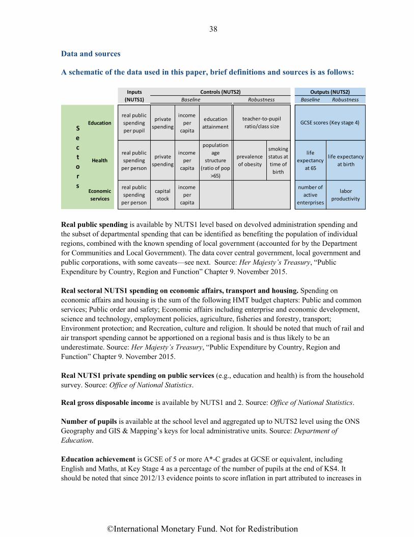
38

Data and sources

A schematic of the data used in this paper, brief definitions and sources is as follows:

Real public spending is available by NUTS1 level based on devolved administration spending and

the subset of departmental spending that can be identified as benefiting the population of individual

regions, combined with the known spending of local government (accounted for by the Department

for Communities and Local Government). The data cover central government, local government and

public corporations, with some caveats—see next. Source: Her Majesty’s Treasury, “Public

Expenditure by Country, Region and Function” Chapter 9. November 2015.

Real sectoral NUTS1 spending on economic affairs, transport and housing. Spending on

economic affairs and housing is the sum of the following HMT budget chapters: Public and common

services; Public order and safety; Economic affairs including enterprise and economic development,

science and technology, employment policies, agriculture, fisheries and forestry, transport;

Environment protection; and Recreation, culture and religion. It should be noted that much of rail and

air transport spending cannot be apportioned on a regional basis and is thus likely to be an

underestimate. Source: Her Majesty’s Treasury, “Public Expenditure by Country, Region and

Function” Chapter 9. November 2015.

Real NUTS1 private spending on public services (e.g., education and health) is from the household

survey. Source: Office of National Statistics.

Real gross disposable income is available by NUTS1 and 2. Source: Office of National Statistics.

Number of pupils is available at the school level and aggregated up to NUTS2 level using the ONS

Geography and GIS & Mapping’s keys for local administrative units. Source: Department of

Education.

Education achievement is GCSE of 5 or more A*-C grades at GCSE or equivalent, including

English and Maths, at Key Stage 4 as a percentage of the number of pupils at the end of KS4. It

should be noted that since 2012/13 evidence points to score inflation in part attributed to increases in

Inputs

(NUTS1) Baseline Robustness

Education

real public

spending

per pupil

private

spending

income

per

capita

education

attainment

Health

real public

spending

per person

private

spending

income

per

capita

population

age

structure

(ratio of pop

>65)

prevalence

of obesity

smoking

status at

time of

birth

life

expectancy

at 65

life expectancy

at birth

Economic

services

real public

spending

per person

capital

stock

income

per

capita

number of

active

enterprises

labor

productivity

Outputs (NUTS2)

S

e

c

t

o

r

s

Baseline Robustness

Controls (NUTS2)

teacher-to-pupil

ratio/class sizeGCSE scores (Key stage 4)


39

the number of non-GCSE results and hence do not reflect a change in education output. However, the

historically consistent Level 2 attainment is used here. Scores are weighted by the number of pupils

for aggregation to the NUTS 2 level using the ONS geography and GIS & Mapping Unit keys.

Source: Department for Education.

Pupil teacher ratio for secondary is available at the NUTS1 level and for years where the data is

missing, the series is spliced with the change in secondary class size from the same source but at the

local school level upward to aggregate up to NUTS1 level using the ONS geography and GIS &

Mapping Unit keys. Source: Department of Education.

Population at NUTS2: Total resident population (midyear population estimates). The estimated

resident population of an area includes all people who usually live there, whatever their nationality.

Members of UK and non-UK armed forces stationed in the UK are included and UK forces stationed

outside the UK are excluded. Students are taken to be resident at their term time address. The data

reflect the new methodology used to calculate migration. Source: Office of National Statistics.

Life expectancy at birth and the age of 65 or at birth. Data is derived from the NUTS2 Annual

Population Survey (APS). Source: Office for National Statistics.

Population age structure (i.e., ratio of population over 65) and density. Data is from the NUTS2

Annual Population Survey (APS) and EuroStat Population Database. Source: Office for National

Statistics and http://ec.europa.eu/eurostat/statistics-

explained/index.php/Population_statistics_at_regional_level

Number of active enterprises: Active enterprises at the NUTS2 level are defined as those that had

either turnover or employment at any time during the reference period. This is a count of active

enterprises in the area. This indicator is a refinement of the indicator covering the number of VAT-

registered businesses at the start of the year: for instance, it recognizes business activity occurring at

any point in the year and it picks up PAYE-registered business as well as VAT-registered businesses.

As a result of this being a more comprehensive measure, the figures are slightly higher than for the

VAT-registered businesses measure. Source: Office for National Statistics. The data is augmented by

splicing with growth rates from the ORBIS firm level database by Bureau van Dijk covering over one

million firms, aggregated up to NUTS2 via a matching of city postcodes.

Regional Gross Fixed Capital Formation. Initial stock of capital for transport and housing is

provided at the NUTS2 level and includes an industry breakdown. Source: Office for National

Statistics.

Labor productivity at NUTS2 level is measured as the change in real output per worker between

2010-14 and 2003-07. Source: Office for National Statistics.

Smoking status at time of delivery. Data is from the website of Public Health of England,

www.phoutcomes.info at the NUTS2 level.

Prevalence of obesity. Data source is the Public Health of England, www.phoutcomes.info at the

NUTS2 level.


http://ec.europa.eu/eurostat/statistics-explained/index.php/Population_statistics_at_regional_level

http://ec.europa.eu/eurostat/statistics-explained/index.php/Population_statistics_at_regional_level

http://www.phoutcomes.info

http://www.phoutcomes.info

40

Tables

Table A.1. Real public spending pre- and post-crisis 1

(Per head for health and economy and per pupil for eduction)

Pre-crisis Post-crisis Change

(2003-07) (2010-14) (percent)

North East

Education 1.80 1.41 -22

Health 2.03 2.65 31

Economic services 2.02 1.95 -4

North West

Education 1.74 1.32 -24

Health 1.60 2.02 27

Economic services 1.58 1.61 1

Yorkshire and the

Humber

Education 1.59 1.42 -11

Health 1.49 1.86 25


Derbyshire and

Nottinghamshire

Education 1.60 1.40 -13

Health 1.33 1.69 27


West Midlands

Education 1.60 1.34 -16

Health 1.45 1.92 32


East of England

Education 1.54 1.32 -14

Health 1.31 1.66 26


South East

Education 1.44 1.33 -7

Health 1.33 1.70 27


South West

Education 1.47 1.42 -3

Health 1.38 1.71 23


Author's estimates based on official and indexed UK data.

1 Aggregated up from NUTS-2 or 3 to NUTS-1 level.


41

Table A.2. Outputs pre- and post-crisis 1

(Per head for health and economy and per pupil for eduction)

Pre-crisis Post-crisis Change

(2003-07) (2010-14) (percent)

North East

Education 38 58 53

Health 18 19 7

Economic services 6 6 8

North West

Education 46 58 27

Health 18 19 6


Yorkshire and the

Humber

Education 44 57 30

Health 19 19 5


Derbyshire and

Nottinghamshire

Education 46 58 26

Health 19 20 5


West Midlands

Education 44 58 33

Health 19 20 6


East of England

Education 52 59 14

Health 19 20 4


South East

Education 50 60 21

Health 19 20 5


South West

Education 46 57 25

Health 20 20 4


Author's estimates based on official UK data.

1 Aggregated up from NUTS-2 or 3 to NUTS-1 level.


4

2

Table A.3. Robustness: Alternative Public Sector Efficiency Indicators 1


Combined

Input-

oriented

Efficiency

Index Education Health Economy

Combined

Input-

oriented

Efficiency

Index



Kent UKJ4 0.94 0.95 1.00 0.963 0.95 0.97 1.00 0.972

Essex UKH3 0.87 0.93 1.00 0.934 0.93 0.97 1.00 0.969





Cumbria UKD1 0.90 0.92 0.76 0.861 0.92 0.89 0.76 0.858

Lancashire UKD4 1.00 1.00 0.84 0.945 1.00 0.86 0.71 0.858

Devon UKK4 0.94 0.91 0.61 0.823 0.91 0.96 0.61 0.829

East Anglia UKH1 0.91 0.89 0.57 0.790 0.89 1.00 0.51 0.802








Cheshire UKD6 0.88 0.97 0.33 0.728 0.97 0.90 0.36 0.743







Merseyside UKD7 0.88 0.96 0.16 0.665 0.96 0.84 0.18 0.662



England average 0.791 0.796

1/ A constant returns to scale technology is assumed in the estimation of the technical efficiency of the production function.



4

3

Table A.4. Robustness: Alternative Public Sector Efficiency Scores Using a Variable Returns Technology

Combined

Efficiency

Index

Combined

Efficiency

Index

Country (NUTS2) Code SCALE SCALE SCALE SCALE SCALE SCALE

Essex UKH3 0.93 0.93 irs 1.00 0.98 irs 1.00 1.00 - 0.977 1.00 0.93 irs 1.00 0.97 irs 1.00 1.00 - 1.000

Surrey, East and West Sussex UKJ2 1.00 0.95 irs 1.00 1.00 - 0.98 0.84 irs 0.994 1.00 0.96 irs 1.00 1.00 - 1.00 0.84 irs 0.998

Berkshire, Buckinghamshire and Oxfordshire UKJ1 1.00 1.00 - 1.00 1.00 irs 0.98 0.38 irs 0.993 1.00 0.99 irs 1.00 0.99 irs 1.00 0.38 irs 0.998

Hampshire and Isle of Wight UKJ3 1.00 0.94 irs 1.00 0.99 irs 0.98 0.85 irs 0.993 1.00 0.92 irs 1.00 0.99 irs 1.00 0.84 irs 0.998

Kent UKJ4 1.00 0.94 irs 1.00 0.97 irs 1.00 1.00 - 0.999 1.00 0.95 irs 1.00 0.97 irs 1.00 1.00 - 0.997

Lincolnshire UKF3 1.00 1.00 - 1.00 0.96 irs 1.00 1.00 - 1.000 0.97 0.99 drs 1.00 0.97 irs 1.00 1.00 - 0.989

Bedfordshire and Hertfordshire UKH2 1.00 1.00 - 1.00 0.98 irs 1.00 0.75 irs 1.000 1.00 1.00 - 1.00 0.99 irs 0.96 0.80 irs 0.986

East Anglia UKH1 0.96 0.95 irs 1.00 1.00 - 1.00 0.57 irs 0.987 1.00 0.89 irs 1.00 1.00 - 0.95 0.54 irs 0.985

Shropshire and Staffordshire UKG2 0.97 0.88 irs 0.96 0.94 irs 0.89 0.49 irs 0.940 0.98 0.96 irs 0.95 0.95 irs 0.97 0.52 irs 0.970

Herefordshire, Worcestershire and Warwickshire UKG1 0.93 0.95 irs 0.96 0.97 irs 0.90 0.66 irs 0.929 0.98 0.97 irs 0.95 0.98 irs 0.97 0.53 irs 0.969

Dorset and Somerset UKK2 0.98 0.95 irs 1.00 0.97 drs 0.96 0.44 irs 0.980 0.93 0.94 irs 1.00 0.98 drs 0.98 0.42 irs 0.969

Cornwall and Isles of Scilly UKK3 1.00 0.89 irs 0.95 0.98 irs 1.00 1.00 - 0.983 0.93 0.96 irs 0.97 0.97 irs 1.00 1.00 - 0.967

Derbyshire and Nottinghamshire UKF1 0.97 0.90 irs 1.00 0.94 irs 0.92 0.45 irs 0.966 0.96 0.99 irs 1.00 0.95 irs 0.94 0.43 irs 0.966

Leicestershire, Rutland and Northamptonshire UKF2 0.94 0.91 irs 1.00 0.96 irs 0.92 0.48 irs 0.956 0.95 0.94 irs 1.00 0.96 irs 0.95 0.48 irs 0.965

West Midlands UKG3 1.00 0.89 irs 0.96 0.93 irs 0.87 0.35 irs 0.944 1.00 1.00 - 0.95 0.94 irs 0.94 0.35 irs 0.964

Devon UKK4 1.00 0.94 irs 0.96 1.00 drs 0.97 0.64 irs 0.975 0.93 0.98 irs 0.97 0.99 irs 0.98 0.63 irs 0.961

South Yorkshire UKE3 1.00 0.81 irs 0.95 0.92 irs 0.87 0.32 irs 0.937 0.99 0.95 irs 0.97 0.92 irs 0.89 0.29 irs 0.952

Gloucestershire, Wiltshire and Bristol/Bath area UKK1 0.98 0.88 irs 0.95 0.99 irs 0.94 0.33 irs 0.956 0.93 0.95 irs 0.97 0.99 irs 0.94 0.34 irs 0.948

North Yorkshire UKE2 1.00 1.00 - 0.95 0.99 irs 0.85 0.50 irs 0.932 1.00 0.98 drs 0.98 0.98 irs 0.87 0.44 irs 0.947

East Yorkshire and Northern Lincolnshire UKE1 0.99 0.88 irs 0.95 0.93 irs 0.88 0.30 irs 0.939 0.96 0.96 irs 0.97 0.93 irs 0.90 0.29 irs 0.946

West Yorkshire UKE4 0.98 0.90 irs 0.95 0.92 irs 0.84 0.34 irs 0.923 0.97 0.98 irs 0.97 0.92 irs 0.87 0.34 irs 0.937

Cumbria UKD1 0.93 0.97 irs 0.90 0.95 irs 0.80 0.95 irs 0.879 1.00 0.92 irs 0.93 0.95 irs 0.79 0.96 irs 0.908

Lancashire UKD4 1.00 1.00 - 0.90 0.92 irs 0.85 0.99 drs 0.917 1.00 1.00 - 0.93 0.92 irs 0.78 0.91 irs 0.905

Cheshire UKD6 0.89 0.98 irs 0.90 0.95 irs 0.78 0.42 irs 0.861 1.00 0.98 irs 0.93 0.96 irs 0.78 0.46 irs 0.905

Merseyside UKD7 0.96 0.91 irs 0.90 0.89 irs 0.77 0.21 irs 0.880 1.00 0.96 irs 0.93 0.90 irs 0.78 0.24 irs 0.904

Greater Manchester UKD3 0.96 0.94 irs 0.90 0.89 irs 0.75 0.19 irs 0.872 1.00 1.00 irs 0.93 0.90 irs 0.75 0.20 irs 0.893

Tees Valley and Durham UKC1 1.00 0.77 irs 0.76 0.90 irs 0.62 0.26 irs 0.792 0.98 1.00 drs 0.79 0.91 irs 0.65 0.32 irs 0.809

Northumberland and Tyne and Wear UKC2 0.97 0.86 irs 0.76 0.89 irs 0.61 0.18 irs 0.781 0.95 1.00 drs 0.79 0.90 irs 0.64 0.19 irs 0.795

England average 0.939 0.947





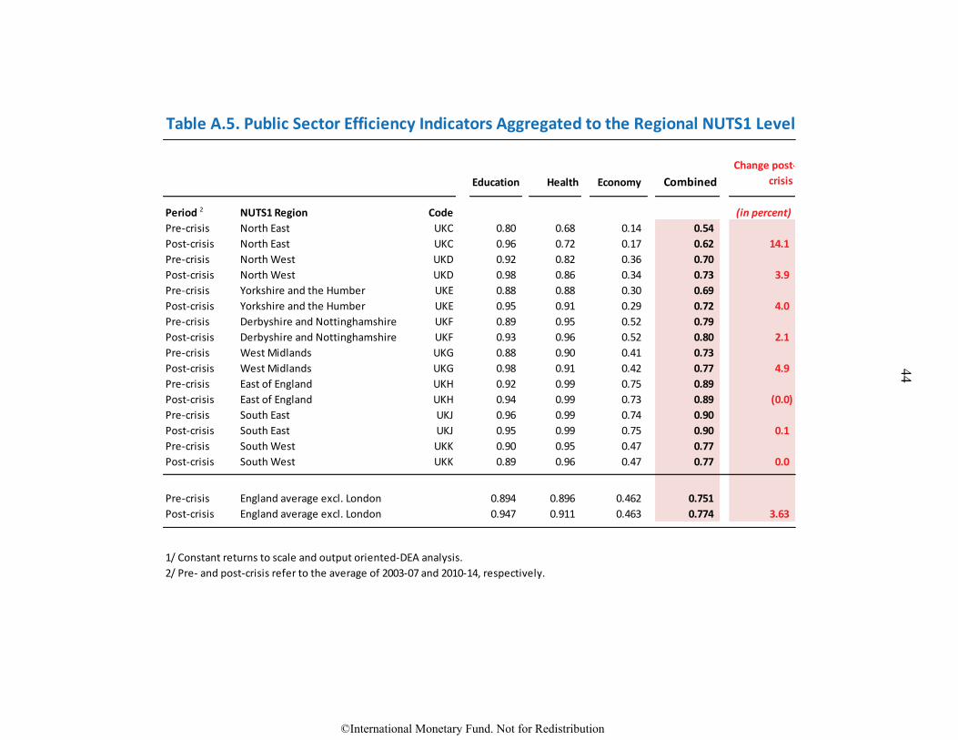
4

4

Table A.5. Public Sector Efficiency Indicators Aggregated to the Regional NUTS1 Level 1

Education Health Economy Combined

Change post-

crisis

Period 2 NUTS1 Region Code (in percent)

Pre-crisis North East UKC 0.80 0.68 0.14 0.54

Post-crisis North East UKC 0.96 0.72 0.17 0.62 14.1

Pre-crisis North West UKD 0.92 0.82 0.36 0.70

Post-crisis North West UKD 0.98 0.86 0.34 0.73 3.9

Pre-crisis Yorkshire and the Humber UKE 0.88 0.88 0.30 0.69

Post-crisis Yorkshire and the Humber UKE 0.95 0.91 0.29 0.72 4.0

Pre-crisis Derbyshire and Nottinghamshire UKF 0.89 0.95 0.52 0.79

Post-crisis Derbyshire and Nottinghamshire UKF 0.93 0.96 0.52 0.80 2.1

Pre-crisis West Midlands UKG 0.88 0.90 0.41 0.73

Post-crisis West Midlands UKG 0.98 0.91 0.42 0.77 4.9

Pre-crisis East of England UKH 0.92 0.99 0.75 0.89

Post-crisis East of England UKH 0.94 0.99 0.73 0.89 (0.0)

Pre-crisis South East UKJ 0.96 0.99 0.74 0.90

Post-crisis South East UKJ 0.95 0.99 0.75 0.90 0.1

Pre-crisis South West UKK 0.90 0.95 0.47 0.77

Post-crisis South West UKK 0.89 0.96 0.47 0.77 0.0

Pre-crisis England average excl. London 0.894 0.896 0.462 0.751

Post-crisis England average excl. London 0.947 0.911 0.463 0.774 3.63

1/ Constant returns to scale and output oriented-DEA analysis.

2/ Pre- and post-crisis refer to the average of 2003-07 and 2010-14, respectively.


Download PDF - IMF eLibrary - International Monetary Fund

Documents