Does Skewness Matter? Evidence from the Index Options Market

DOES SKEWNESS MATTER? EVIDENCE FROM THE INDEX OPTIONS MARKET

Madhu Kalimipallia

School of Business and EconomicsWilfrid Laurier University

Waterloo, Ontario, Canada N2L 3C5Tel: 519-884-0710 (ext. 2187)

[email protected]

Ranjini Sivakumar b

Centre for Advanced Studies in FinanceSchool of AccountancyUniversity of Waterloo

Waterloo, Ontario, Canada N2L 3G1Tel: 519-888-4567 (ext. 5703)

[email protected]

(This draft November 8, 2002)

Key Words: conditional volatility and skewness, option pricing biases, at-the-moneydelta-neutral strips, straps and straddles

JEL Classification: G10, G14

a The first author acknowledges support from a Wilfrid Laurier University post-doctoral grant.b Corresponding author

Does Skewness Matter? Evidence from the Index Options Market

ABSTRACT

We model the temporal properties of the first three moments of asset returns and examinewhether incorporating time varying skewness in the underlying asset returns leads toprofitable strategies using at-the-money S&P 500 index options. We devise trading rulesthat incorporate the skewness forecast to trade at-the-money delta-neutral strips, strapsand straddles. We find that a simulated trading strategy using a model with bothconditional volatility and skewness outperforms the GARCH model before and afteradjusting for transaction costs. The results indicate that index option prices forat-the-money options do not reflect time varying skewness. The evidence suggests thatmispricing of options may cause the negative skewness in the implicit risk-neutraldistribution in option prices.

Does Skewness Matter? Evidence from the Index Options Market

1. INTRODUCTION:

Existing literature has documented significant time varying skewness in stock index

returns (Harvey and Siddique, 1999 and 2000 and Hansen, 1994). The natural

development of skewness persistence models is an extension of volatility persistence

models and a direct consequence of asset pricing equations that contain third central

return moments. Harvey and Siddique (1999) find strong evidence for time varying

variance and skewness in monthly and weekly stock index data. Inclusion of conditional

skewness is found to attenuate asymmetric variance and seasonality effects in conditional

moments and lead to lower persistence in the variance equation.

There is significant empirical evidence (see e.g. Bates, 1996b for a summary) that the

Black-Scholes valuation model exhibits pricing biases across moneyness and maturity.

Bates (1991) shows that out-of-the-money (OTM) puts became very expensive relative to

OTM money calls during the year preceding the stock market crash in October 1987 as

skewness premium implicit in OTM money options on S & P 500 futures became

significantly negative. The negative skewness premium results in a “smirk” pattern in

index volatilities. In addition, Bates (2000) documents significant time varying skewness

in stock index option data.

The interesting question is how does the conditional skewness in the asset returns

affect the underlying risk neutral pricing distribution used in option valuation? Jackwerth

and Rubinstein (1996) document that in the pre 1987 period, both the risk-neutral

distribution (option implied distribution) and the actual distribution of S&P 500 returns

are about lognormal. However in the post 1987 period, while the actual distribution

2

looks about lognormal again, the risk-neutral distribution is left-skewed and leptokurtic.

Bates (2000) suggests three explanations for the negative skewness in the implicit

risk-neutral distribution. The first is that investors view the underlying stochastic process

for S&P 500 returns has changed, the second is a change in investor’s risk aversion and

the third reason being a mispricing of post-crash options. Bakshi, Cao and Chen (1997)

and Bates (2000) among others look at the first explanation and propose option valuation

models that incorporate the asymmetry in the risk neutral pricing distribution. Jackwerth

(2000) looks at the second explanation. He empirically derives risk aversion functions

implied by option prices and realized returns on the S&P500 index for the period 1986-

1995. In the post 1987 period, he finds negative risk aversion functions that are

inconsistent with economic theory and concludes that the market misprices the options.

Bakshi et al. (1997) examine options on the S&P 500 index during the period

1988-1991. They compare the Black-Scholes (BS) model, the stochastic volatility model

(SV), the stochastic volatility stochastic interest (SVSI) model and the stochastic

volatility random jump (SVJ) model. Their empirical evidence suggests that overall, a

model with stochastic volatility and random jumps is superior to the Black-Scholes

model. Interestingly they find that for at-the-money (ATM) options, the Black Scholes

model does as well as the other models. Their in-sample analysis suggests that for ATM

options, the pricing models have similar implied-volatility values. In the out-of-sample

cross-sectional performance, they find that ATM call options valued using the Black-

Scholes model do not show any maturity-related bias. Their analysis of hedging errors

suggests that except for in the money (ITM) options, hedging errors using the Black-

Scholes model are indistinguishable from those obtained using the other models.

3

In this paper, we investigate whether it is mispricing that causes the negative

skewness in the implicit risk-neutral distribution. Specifically, we examine if options are

mispriced because they ignore the embedded skewness in the underlying asset’s returns.

We model the temporal properties of the first three moments of asset returns following

Hansen (1994) and Harvey and Siddique (1999) and examine if incorporating time

varying skewness in underlying asset returns leads to profitable option based strategies.

We examine S&P500 index options data during the period November 1998 to December

2001. For this study, it appears that the hedging yardstick would be most appropriate.

Based on hedging errors, Bakshi et al. (1997) suggests that the Black-Scholes model

would work as well as the other models for pricing ATM options. Hence, we assume that

the Black-Scholes model is the appropriate option valuation model and assess whether

trading rules that incorporate the skewness forecasts of asset returns lead to profitable

strategies using ATM options.

We use a framework proposed by Noh, Engle and Kane (1994) to estimate the profits

from the options trading strategies. Noh et al. (1994) show that simple GARCH models

(that incorporate time varying volatility) outperform implied volatility models for

investors trading in at-the-money straddles, after accounting for transaction costs. We

use the GARCHS (GARCH with conditional skewness) model as in Hansen (1994) and

obtain the latent volatility and skewness from spot data. The GARCHS trading strategy

leads to trading in a strip or a strap. When conditional skewness is indeed constant, the

GARCHS reduces to a GARCH model and both models should yield similar returns.

4

We find that a simulated trading strategy using the GARCHS model outperforms the

GARCH model before and after adjusting for transaction costs. The empirical evidence

indicates that index option prices for ATM options do not reflect time varying skewness..

This paper is organized as follows. In section 2, we provide a brief literature review.

In section 3, we describe the data and provide the sample description statistics. In section

4, we discuss the empirical methodology and present the results on the volatility models.

In the next section we discuss the trading strategies. In section 6, we present the results

on the trading strategies. Section 7 concludes.

2. BACKGROUND AND LITERATURE REVIEW:

What causes skewness or asymmetry in returns? There are at least four possible

explanations in the literature. The first explanation is the “leverage effect” whereby a

drop in stock price leads to higher operating and financial leverage and hence high

volatility in subsequent returns (Black, 1976). The second is based on the “volatility

feedback mechanism” whereby the direct effect of a positive shock on volatility is

mitigated by an increase in risk premium, while in the presence of a negative shock both

direct and indirect effects work to increase the risk premium. Negative dividend shocks

leads to higher firm volatility, which in turn leads to higher required rates of return on

equity and hence lower stock prices (Campbell and Hentschel, 1992). The third

explanation is based on a possible bursting of a “bubble”, a low probability scenario with

large negative consequences (Blanchard and Watson, 1982). Finally investor

heterogeneity and short sale constraints of investors explain skewness. When trading

volume is high, differences of opinion are also high and bearish investors with short-sale

5

constraints are forced to a corner solution. When bad news hits the market, the hidden

information of the bearish investors is released to the market and this in turn induces

negative skewness in the subsequent periods (Chen, Hong and Stein, 1999).

Hansen (1994) provides a model of skewness evolution in the context of conditional

density estimation using a skewed Student-t distribution. He proposes a model of

skewness that evolves much like a GARCH process in squares of residuals and applies

the approach to the estimation of US Treasury securities and the US dollar/Swiss Franc

exchange rate. He finds evidence of skewness persistence. Harvey and Siddique (1999)

adapt Hansen's approach to a wide number of daily and monthly equity return series.

Harvey and Siddique (2000) introduce skewness in the CAPM framework by expressing

the stochastic discount factor or inter-temporal marginal rate of substitution as a quadratic

function of the market return. They find that the coskewness factor (defined as that part

of an asset’s skewness that is related to market portfolio’s skewness) has value in cross-

sectional CAPM regressions across assets. This is in addition to size and book-to-market

factors that were proposed by Fama and French (1992). The momentum effect in

portfolios is found to be related to the systematic skewness factor. The question that

follows is what does a negatively skewed empirical distribution imply for the implicit

risk-neutral distribution in option prices. We next review some of the options related

literature that looks at this issue.

Bates (1991) shows that the out-of-the money puts became very expensive during the

latter half of 1986, remained so until early 1987 and again during August of 1987 as

skewness premium implicit in out-of-the money options on S & P 500 futures became

significantly negative. No such effects were found during the months immediately

6

preceding the October 1987 crash. Following the 1987 crash, the negative skewness

premium continued to be significant till the end of 1987. Citing the specification of the

underlying stochastic process as a possible reason for the skewness premium, the paper

introduces a diffusion model with systemic jump risk to capture the time varying

skewness in the data.

Using a jump-diffusion model, Bates (1996a) finds a significant positive implicit

skewness in currency options on Deutsche mark during the period 1984-1987, but not

from 1988-1991. The author shows that a SV model with jumps can explain high

kurtosis and skewness across different option maturities. Bakshi et al. (1997) propose an

option pricing model with stochastic volatility, stochastic interest rates and random

jumps. Their empirical evidence suggests that a model with stochastic volatility and

random jumps is superior to the Black-Scholes model. Bates (2000) again considers a

SV model now with time varying jumps to explain the skewness implicit in the S & P

500 futures option markets. The paper shows that models with SV or a negative

correlation between returns and volatility alone are not sufficient to generate the high

negative skewness or high volatility of volatility in the data.

In related research on the underlying stochastic process, Heston and Nandi (2000)

point out that a GARCH option valuation model that captures the negative correlation of

spot returns with volatility and the historical information in volatility model results in

reduced moneyness and maturity biases in option valuation. They also show that the

GARCH option valuation model is superior to an ad-hoc (smoothed) Black-Scholes

model proposed by Dumas, Fleming and Whaley (1998).

7

Chen, Hong and Stein (1999) using a panel data of U.S firms, find that negative

skewness is most pronounced in stocks with high past trading volume and returns and for

larger sized stocks. Bakshi, Kapadia and Madan (2000) show that risk-neutral

distributions for individual stocks differ from that of the market index by being far less

negatively skewed and substantially more volatile. Jackwerth (2000) rules out changes in

investor risk aversion as a reason for the negative skewness and suggests mispricing as a

possible reason. We explore the mispricing explanation in this paper.

3. DATA AND SAMPLING PROCEDURE:

In this study, we use S&P 500 daily options data and daily index levels from October

1998 to December 2001. We examine the S&P500 index options data because these

options are widely traded. For each day, we use the closing option price and the closing

index level as reported in the Datastream International database. We assume that the

S&P 500 daily dividend yield interpolated to match the maturity of the option contract is

a reasonable proxy for the dividends paid on each option contract. We use the six-month

Treasury-bill rate as a proxy for the risk-free rate in the Black-Scholes valuation model.

Following Bakshi et al. (1997), options with moneyness (strike price/index level) in

the range 0.97 to 1.03 are deemed as at-the-money options and are included. Options

with maturity less than fifteen days and greater than 180 days are excluded. Only options

with daily volumes greater than 100 are retained. For a given exercise price and

maturity, options that have both put and call prices are retained. Options that violate the

put-call parity relationship are excluded. Since the option market closes after the stock

market, the option holder has a wildcard option. As in Noh et al. (1994), we ignore the

8

wildcard option, understating the profits from the trading rules. Based on these criteria,

our sample consists of 2,279 call-put options pairs on 522 trading days.

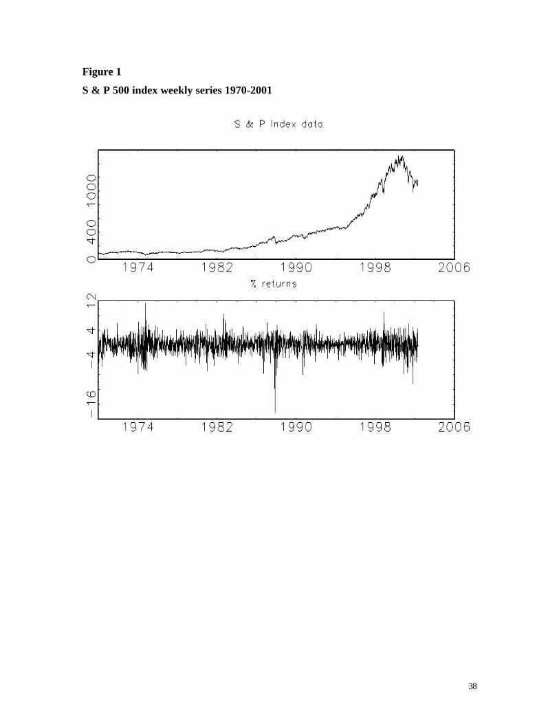
Figure 1 presents the weekly S & P 500 price index and returns for the period

1970-2001. We see that the index surged from mid 90’s onwards and peaked in the year

2000 followed by a decline.

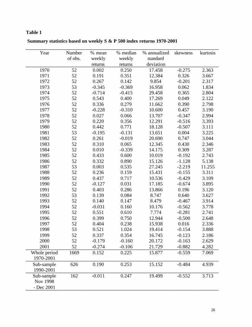
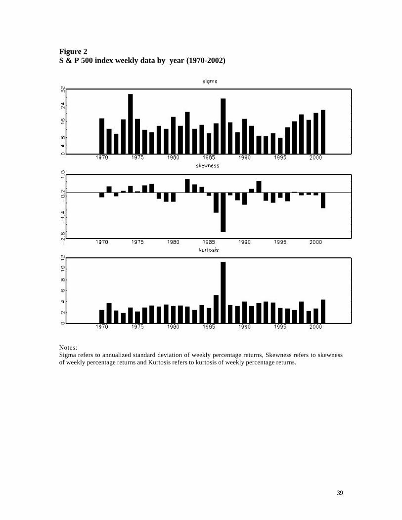
Table 1 presents the summary statistics of the weekly S & P 500 index data for the

period 1970-2001. In general we see that volatility, skewness and kurtosis have been

varying over time and have been high during the periods of oil shocks in the 1970s, the

1987 crash period and more recently since the year 2000. The sample period for our

index options (Nov 1998-December 2001) seems to be characterized by particularly high

volatility compared to the historical average. Figure 2 reveals that (unconditional)

market volatility has been steadily growing since mid 90s. Negative skewness has

become more prominent after the 1987 crash and more so during 2001. The kurtosis has

remained steady except for the crash year.

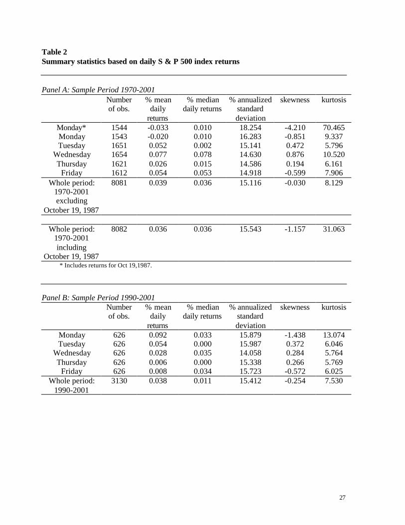
Table 2 presents the summary statistics of the daily S & P 500 index data for the

period 1970-2001 and the sub-period 1990-2001. In general for the full sample period,

we see that volatility, skewness and kurtosis vary over the week and are usually high on

Mondays compared to the rest of the week. From, Panel B we observe that for the period

1990-2001, a period following the October 1987 crash, the skewness and kurtosis are

high on Mondays, while the volatility is similar to the volatility on other days of the

week. Similar patterns are visible in Figure 3.

Figure 4 presents the density functions of the weekly and daily time series index data.

We see large negative skewness and fat tails in the data. In particular, we observe high

9

negative skewness in weekly data and high kurtosis in daily data. This is also confirmed

by Tables 1 and 2.

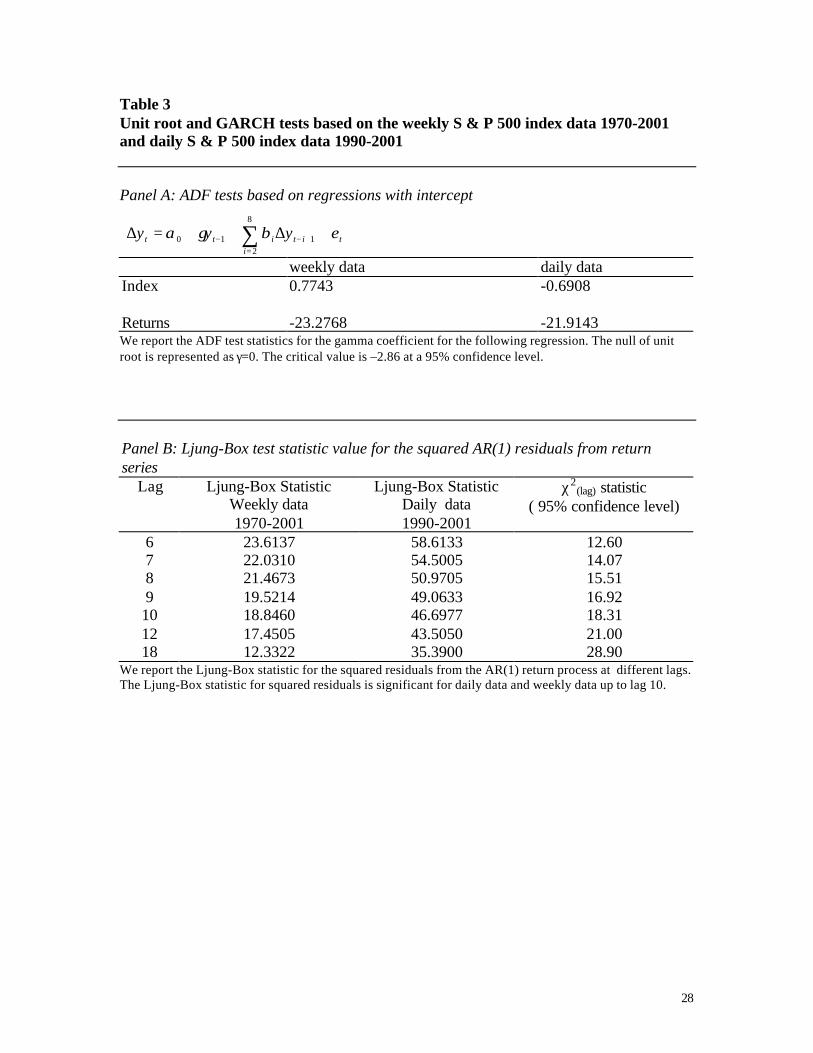
Panel A in Table 3 presents the augmented Dickey-Fuller unit root tests for the daily

and weekly price index data. We cannot reject the unit root null hypothesis for the index

data at both the daily and weekly frequencies. The first differencing however seems to

gives us the stationary return series. Panel B presents the Ljung-Box statistics for the

squared AR(1) return residuals. They indicate high auto-correlations in the daily and

weekly data that imply time dependence in higher order moments such as GARCH

effects.

4. RESULTS FROM CONDITIONAL VOLATILITY MODELS:

In this section we describe the conditional volatility and skewness models and their

results based on the time series index data. We use the GARCH (1,1)-in-mean model

with leverage and Monday effects and time varying conditional skewness and degrees of

freedom – referred to as GARCHS (1,1) model as the omnibus specification. Hansen

(1994) obtains a density function for a random variable driven by its skewness and

degrees of freedom (df) in addition to the first two moments. The details are provided in

Appendix 1. This specification is very general and it reduces to several known

specifications as special cases. The GARCHS(1,1) specification (denoted as Model 4 in

our tables ) is described below.

10

Model 4:

The distribution g(-) for the standardized residual error term is described in the appendix.

Other models (with the exception of the EGARCH model) can be obtained as special

cases of Model 4. The details of these models are provided in Appendix II. Model 1 is

the GARCH (1,1)-M model with leverage and Monday effects and is obtained by setting

df in Model 4 to a high number above 30 and by constraining skewness to zero. Model 2

is the EGARCH (1,1)-M with Monday effect. Model 3 is obtained by constraining the

conditional df and skewness equations in Model 4 to only have intercepts.

Table 4 presents the results for weekly index returns for the period 1970-2001. From

panel A in table 4 we see that variables in the mean equation are generally insignificant

for all models except for model 3 where the lag of returns is significant. In particular,

there is weak evidence of risk premium in the mean equation. However we find high

persistence in the variance equation and a strong evidence for leverage in the data. In

model 3, the intercept in the df equation denoting the average fatness in tails is not very

prominent, while the skewness intercept is highly significant.. In model 4, fat tails seem

to be driven by large (perhaps negative) shocks to the returns as evidenced by the

otherwise 0

Monday if 1

0 10 0

),|(~)|( ,

ˆˆ

1

11

212110

212110

42

1132

12110

1

12110

=

=

<≥

=

++=

++=

++++=

Ω=

+++=

−

−−

−−

−−

−−−−

−

−−

tMon

uifuif

d

uuSk

uudf

Monu duhh

Zghu

uhrr

tt

tt

ttt

ttt

tttttt

ttttt

tttt

δδδ

γγγ

βββββ

ληεε

ααα

11

significant coefficient on lagged squared residual in the df. Conditional skewness effects

are significant. There is a large negative skewness and it is time varying.

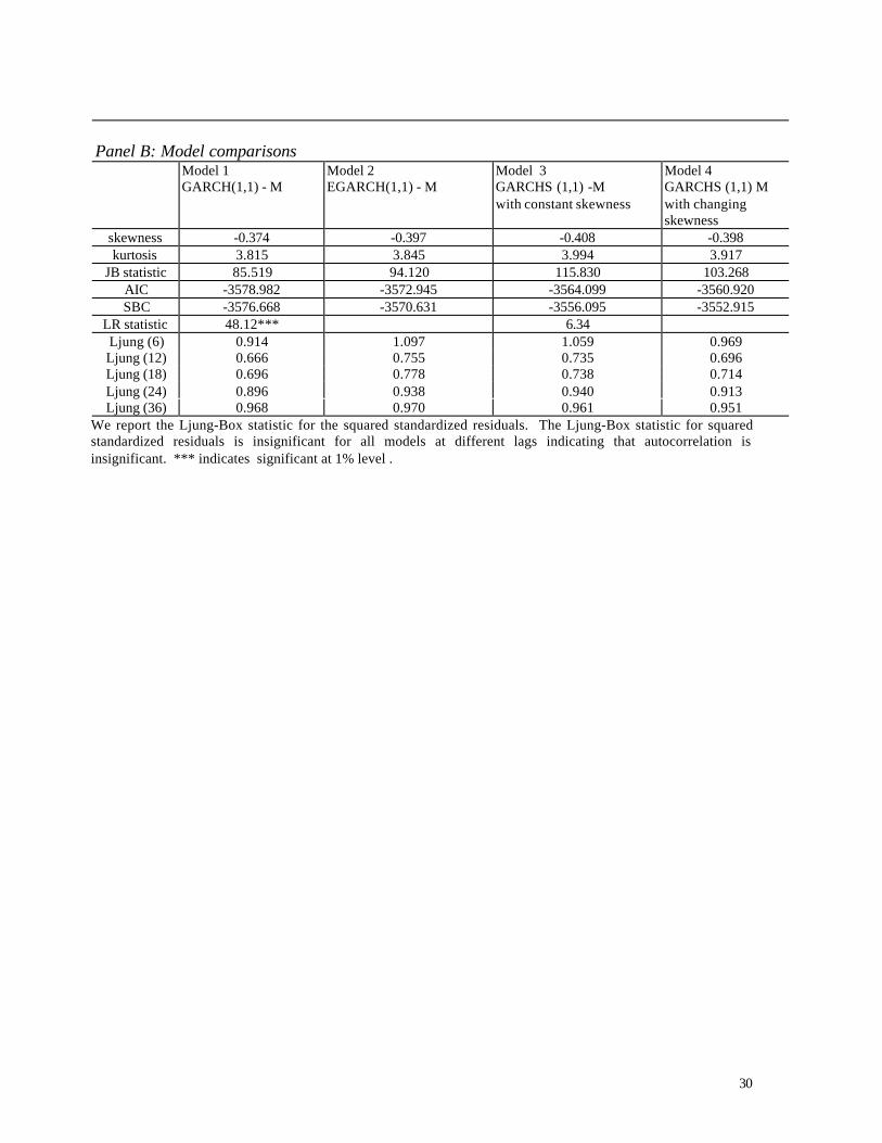
From the last row in panel A, we note that Model 4 outperforms the other models in

terms of the highest likelihood. From panel B, we observe that Model 4 is the best

specification based on the AIC and SBC criteria. Models 1 and 2 come out as winners in

terms of normality of standardized residuals captured in the Jarque-Bera metric.

Conditional skewness and constant skewness models do not seem to be particularly

successful in correcting for non-normality in the standardized residuals. The likelihood

ratio metric for nested specifications confirms that Model 4 is a definite improvement

over Model 1. However there is not much improvement over Model 3. The last result

implies that time varying df and skewness in terms of lagged residuals do not add much

information beyond what is already contained in their respective intercepts. The Ljung-

Box statistic for squared standardized residuals is insignificant for all models indicating

that autocorrelation is insignificant. In particular, Ljung-Box statistics show that Model 2

with embedded leverage effect has the least correlation in higher moments. Model 4

seems to perform better at higher lags. This implies that conditional skewness and df

effects resulting in higher-order return correlations are less prominent in the weekly data.

Table 5 presents the results for daily index data for the period 1990-2001. From

panel A in table 5, we see that lagged returns are highly significant in all models. As

observed in weekly data there is weak evidence of risk premium in the mean equation.

Compared to the weekly data there is even a high persistence in the variance equation and

strong evidence for the leverage effect. The coefficient on lagged squared residuals in

the variance equation is insignificant indicating that mainly large negative shocks, as

12

captured in the leverage effect drive the volatility. In Models 3 and 4, the intercept in the

df equation is now highly significant. Unlike the weekly data, daily data has very

significant fatness in tails. However, there is not much evidence of time varying kurtosis

as the residual terms are insignificant. As in weekly data, conditional skewness effects

are also very significant. The main difference is in the size of the intercept term in the

skewness equation; skewness in the daily data is much less negative and significant

compared to the weekly data. Higher kurtosis and lower negative skewness in daily

index series relative to the weekly data is consistent with what we observe in tables 1-2

and figure 1. Monday effects are generally insignificant.

Panels A and B (table 5) indicate that Model 4 again outperforms the other models in

terms of the highest likelihood, AIC and SBC values. Model 2 is the best model in terms

of the Jarque-Bera metrics as before. The likelihood ratio test for nested specifications

shows that Model 4 is a definite improvement over models 1 and 3. There seems to be

incremental information in conditional skewness in daily data, in contrast to the results in

the weekly data. Just as in weekly data, the Ljung-Box statistic for squared standardized

residuals is insignificant for all models indicating that autocorrelation is insignificant. In

particular, Ljung-Box statistics show that Model 4 has the least correlation among higher-

order moments for lags up to 18. This implies that conditional skewness and df effects

that lead to return correlations are more prominent in the daily data. Model 1 seems to

perform better at lags beyond 18.

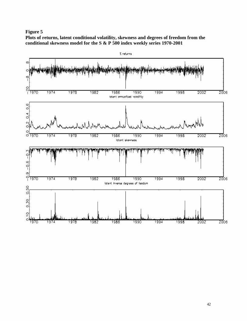
Figure 5 plots returns, latent conditional volatility, skewness and inverse degrees of

freedom from the conditional skewness model (Model 4) for the S & P 500 index weekly

series 1970-2001 and Figure 6 has a similar plot for the daily index data for the period

13

1990-2001. The lower the df the greater is the fatness in the tails of return distributions.

In general we find that periods of high volatility are also periods of high negative

skewness and fatness in the return distributions. The 1970s oil shocks, 1987 crash, 1990

Gulf war, 1997-98 Asian crisis, 1998-99 Russian crisis and the 2001 burst of the

technology bubble are all periods of high return shocks and also of high volatility and

skewness. Negative skewness became more pronounced i.e. underlying markets became

more pessimistic in these shock periods. These were also the periods when the return

distributions became very fat tailed. Comparing the latent skewness from weekly and

daily data we find that negative skewness is more pronounced in weekly data. This

follows from the fact that the skewness intercept for weekly data is more negative and

significant than for daily data (see Tables 4-5).

5. TRADING STRATEGIES:

We use the framework proposed by Noh, Engle and Kane (1994) to estimate the

profits from the options trading strategies. These strategies involve trading in

delta-neutral at-the-money straddles, strips and straps. Figure 7 depicts the profit patterns

in these strategies. In this paper, we argue that the investor can use the forecast of

skewness to formulate profitable trading strategies in strips or straps or straddles.

We forecast the volatility using the conditional volatility models. The GARCHS

model provides a forecast of skewness as well. While the GARCH model leads to

trading in a straddle, the GARCHS trading strategy leads to trading in strips or straps as

well. When conditional skewness is indeed constant, the GARCHS reduces to a GARCH

model and both models should yield similar returns. We use the volatility forecasts to

14

price the straddles, strips and straps using the Black-Scholes model. We use at-the-

money options because Bakshi et al.’s (1997) paper suggests that the Black-Scholes

model works well for pricing ATM options. Since we use delta neutral positions, we also

do not need to delta-hedge. We next describe the strategies and the trading rules.

A. Trading only in straddles:

1. First estimate each time series model (models 1 to 4) and obtain the average

volatility forecast for each model at time t for the remaining period to maturity

of an option.

2. Using the in-sample daily volatility forecasts from step 1, obtain the delta-

neutral (DN) straddle for each trading day.

3. Next plug the time t in-sample daily volatility forecasts from step 1 into the

BS option model and obtain the ATM DN straddle prices as in Noh, Engle

and Kane (1994).

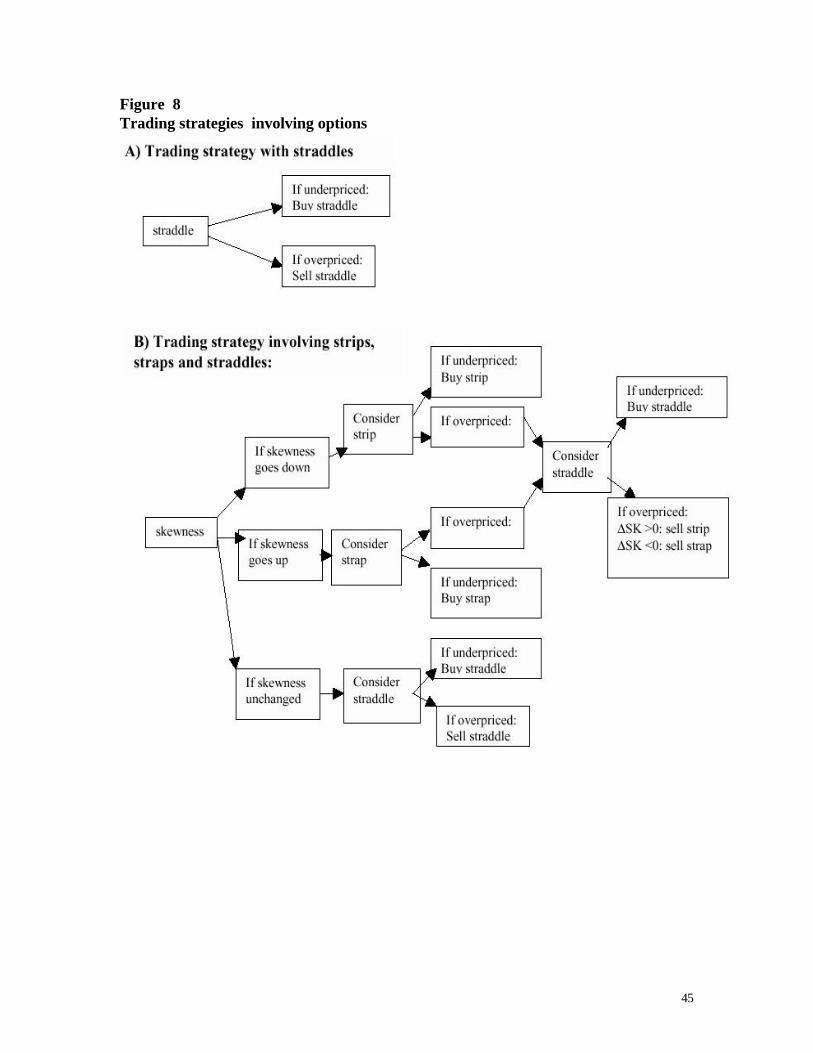
4. Finally buy or sell the straddle depending on whether it is under or over-

priced. When the straddle is sold, the agent invests the proceeds in a risk-free

asset. Figure 8a illustrates this straddle trading strategy.

5. This strategy is implemented each day.

6. For all trades, we apply a filter as in Noh et al. (1994). The agent trades only

when the absolute price difference between model and market price is

expected to exceed $0.25 or $0.50.

7. We also evaluate the strategies after imposing trading costs of 0.5% of the

price of the straddle. We assume that an investor would trade for an amount

15

exceeding $10,000 and would pay a commission amounting to $120 + 0.0025

of the dollar amount as per a standard commission schedule (see Hull (2000)

p. 160).

8. The rate of returns are calculated as follows:

Return on buying a straddle = 1t1t

1t1tttPC

PCPC

−−

−−+

−−+

Return on selling a straddle = f1t1t

1t1ttt rPC

)PCPC(+

+−−+−

−−

−−

B. Trading in strips, straps and straddles:

Next we turn to delta-neutral strips, straps and straddles. Figure 8b shows the

differences between the straddles only strategy and that based on strips, straps and

straddles. With strips and straps we need estimates of the next period skewness. We

have a much larger set of trading opportunities now. These are described below (all

strips, straps and straddles are delta neutral ):

1. First estimate skewness time series model (models 3 and 4) and obtain the

average volatility forecast for each model at time t for the remaining period to

maturity of an option.

2. Using the in-sample daily volatility forecasts from step 1 obtain the delta-neutral

(DN) strip, strap and straddle for each trading day.

3. Next plug the time t in-sample daily volatility forecasts from step 1 into BS option

model and obtain the ATM DN strip, strap and straddle prices.

16

4. Finally buy or sell the strips, straps and straddles following the trading strategy

outlined below

• If skewness is likely to go down and the strip is under priced, buy the strip

• If skewness is likely to go up and the strap is under priced, buy the strap.

• If skewness is likely to go down and the strip is overpriced, buy the straddle if

it is under priced. If the straddle is not under priced, sell the strap.

• If skewness is likely to go up and strap is overpriced, buy the straddle if it is

under priced. If the straddle is not under priced, sell the strip.

• If skewness is likely to stay unchanged and the straddle is under priced, buy

the straddle.

In all the above trades, we apply the skewness filter in that we trade in strips an straps

only if skewness changes by more than plus (or minus) one standard deviation around the

mean, where mean and standard deviation refer to those of first differences in skewness.

While straddles traders have only the last trading strategy; traders using strips, straps and

straddles on the other hand have access to an added list of strategies from 1-4. We follow

the procedure below to compute returns from ATM delta-neutral strips, straps and

straddles :

5. The rate of returns are calculated as follows:

Return on buying a strip = 1t1t

1t1tttP2C

P2CP2C

−−

−−+

−−+

Return on selling a strip = f1t1t

1t1ttt rP2C

)P2CP2C(+

+−−+−

−−

−−

Return on buying a strip = 1t1t

1t1tttPC2

PC2PC2

−−

−−+

−−+

17

Return on selling a strip = f1t1t

1t1ttt rPC2

)PC2PC2(+

+−−+−

−−

−−

6. The returns are calculated after imposing the filters and before and after

transaction costs.

6. RESULTS FOR OPTION TRADING STRATEGIES:

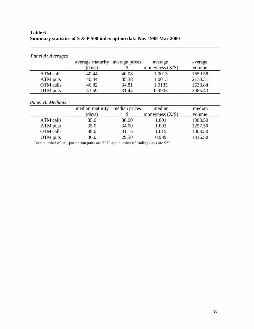
Table 6 presents the summary statistics of S & P 500 index options data for the period

Nov 1998-December 2001. In general puts are cheaper relative to calls and trade more

heavily. At-the-money options (ATMs) also seem to have a shorter maturity compared to

out-of the money options (OTMs).

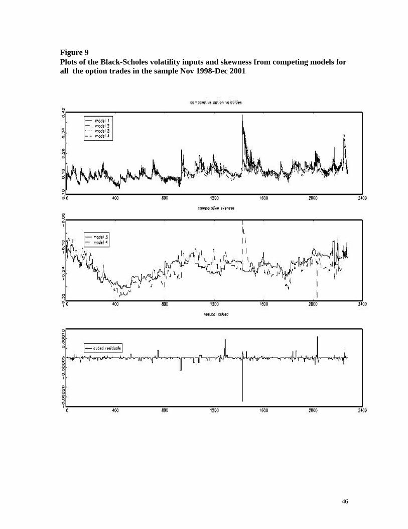
Figure 9 plots the Black-Scholes volatility inputs and skewness from competing

models for all the option trades in the sample. We find that Black-Scholes volatility

inputs are similar across models with EGARCH giving lower volatility inputs than other

models. The Model 4 skewness forecast are more sensitive to shocks than Model 3. The

Model 4 skewness forecast closely tracks the cubed residuals. .

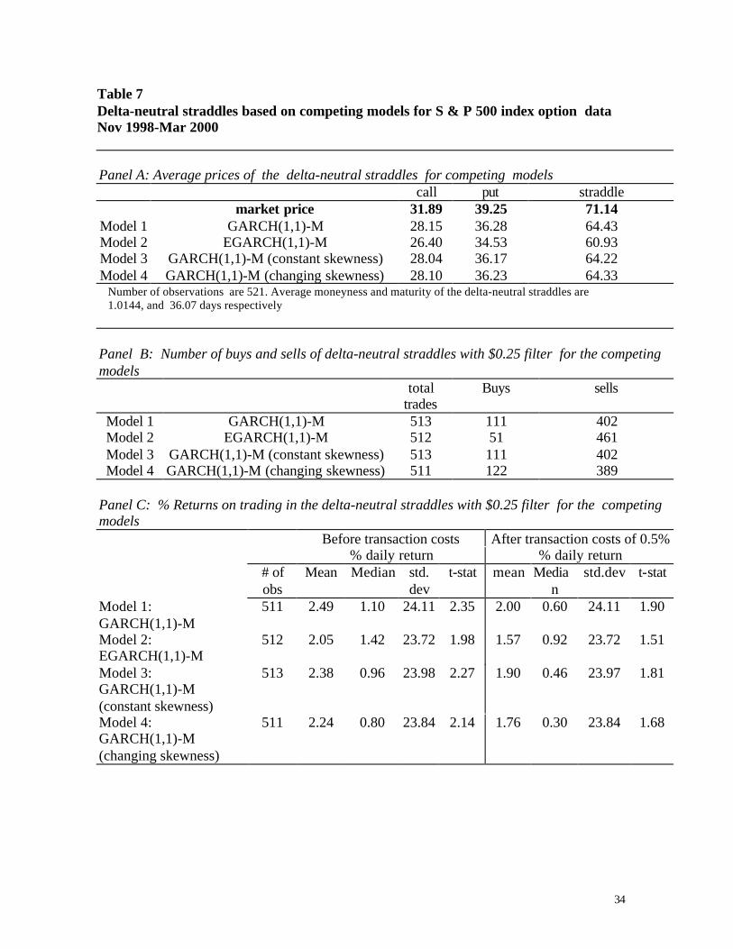
Table 7 presents the results for delta-neutral straddles based on competing models

based on the above procedure. We use the S & P 500 index options data for the period

Nov 1998-December 2001. Panel A shows us that the average moneyness (X/S) is

1.0144, hence put prices are much higher relative to the call prices. Model 1

(GARCH (1,1)-M with normal distribution for the error term) comes closest to the actual

market prices of calls and put and straddles, while the EGARCH (1,1)-M gives us the

lower bounds. In general the model prices are much lower compared to the option prices

implying that options are over priced. Panel B gives us the number of buys and sells of

the delta-neutral straddles for competing models. We find that in general straddles are

18

sold in about 75% of the trades. Model 4 with time-varying volatility and skewness

involves the least short positions in straddles.

Panel C (table 7) presents percentage returns on trading in the delta-neutral straddles

for competing models using a $0.25 filter for stock price changes. Trading takes place

only if the absolute price deviation is greater than $0.25. We find that Model 1(GARCH)

performs best both before and after-transaction costs followed by the models that

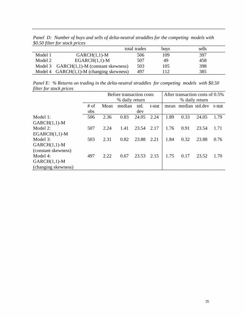
incorporate skewness. Panels D and E (table 7) replicate Panels B and C results using a $

0.50-filter rule for stock price changes. We find that the numbers of trades are now lower

because of attrition due to the filter rule; the straddles are still sold more often than they

are bought. As before, Model 1 outperforms all others before and after 0.25% transaction

costs. In both panels, the median returns indicate that the EGARCH model performs

best.

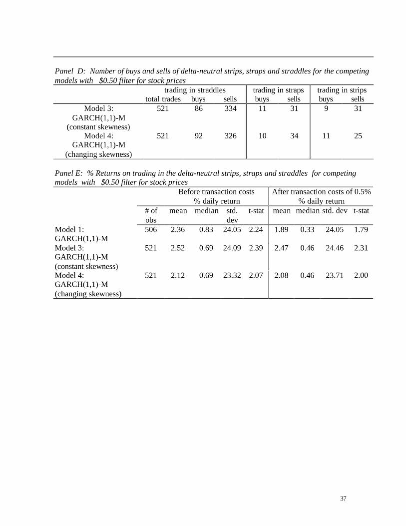
Table 8 presents the results for delta-neutral strips and straps and straddles based on

competing models for S & P 500 index options data. Panel A shows that in general the

model prices are much lower compared to the option prices implying that options are

over priced. Panel B (table 8) gives us the number of buys and sells of the delta- neutral

strategies for competing models. In general we find that strips, straps and straddles are

sold more often than purchased. The buys and sells are now spread over strips, straps and

straddles unlike straddles only in table 7. Since we imposed a skewness filter, we find

that less than 20% of the trades are in straps and straps.

Panel C (table 8) presents percentage returns on trading in the delta-neutral strategies

for the competing models. We find that mean returns from both conditional skewness

models, are higher than those reported in table 7 both before and after transaction costs.

19

The t-statistics indicate that the returns from the strategy are significantly different from

zero.

Panels D and E (table 8) replicate panels B and C results using a $ 0.50-filter rule for

stock price changes. We find that the numbers of trades are now lower because of

attrition due to the filter rule; the number of sells still overwhelms the number of buys.

Returns from both skewness models still outperform all others reported in table 7

particularly after transaction costs.

6. SUMMARY AND CONCLUSIONS:

We investigate whether it is mispricing that causes the negative skewness in the

implicit risk-neutral distribution in S&P 500 index option prices. We model the temporal

properties of the first three moments of asset returns following Hansen (1994) and

Harvey and Siddique (1999) and examine if incorporating time varying skewness in

underlying asset returns leads to profitable strategies using at-the-money options. We

find that a simulated trading strategy using the GARCHS (skewness) model outperforms

the GARCH model both before and after adjusting for transaction costs. The empirical

evidence indicates that index option prices for ATM options do not reflect time varying

skewness. Our results suggest that mispricing of options may cause the negative

skewness in the implicit risk-neutral distribution in option prices.

20

Appendix I: Conditional Skewness Model:

The GARCHS (1,1) specification for the conditional mean, conditional variance andconditional skewness, where the error term in the mean has a skewed conditional studentt distribution with changing degrees of freedom, is as follows:

Conditional mean: t1t21t10t uhˆrˆˆr +++= −− ααα

where, ttt hu ε= and ( )ληΩε ,|zg~| 1tt −

where g ( ) is as described below.

Conditional variance: 21t1t3

21t21t10t uduhh −−−− +++= ββββ

where,

<

≥=

−

−− 0uif1

0uif0d

1t

1t1t

Conditional skewness 21t21t10t uSk −− ++= δεδδ

Degrees of freedom: 21t21t10t udf −− ++= γεγγ where ∞<< df2

The likelihood function for the skewed t distribution (Hansen 1994) is:

−≥

++

−+×

−<

−+

−+×

= +−

+−

ba

z1

abz2

11cb

ba

z1

abz2

11cb

),|z(g

2

12

21

2

η

η

λη

ληλη

where ηstands for degrees of freedom and is bounded as ∞<< η2 and λ is the skewness

parameter and is bounded as 11 <<− λ . Further the constants a, b and c are as defined

below.

21

−

+

=

−+=

−−

=

2)2(

21

c

a31b

12

c4a

222

ηΓηπ

ηΓ

λ

ηη

λ

Hansen (1994) show that this density function has a zero mean and unit variance.

Setting λ to zero gives us a regular t-distribution and setting η to a high number over 30

and λ to zero gives us a regular standard normal distribution.

22

Appendix II: Volatility and Skewness Models Tested

1. GARCH(1,1)-M with leverage and Monday effect:

2. E-GARCH(1,1) with Monday effect:

3. GARCHS(1,1) – M with leverage and Monday effects with constant skewness:

=

=

<

≥=

++++=

Ω=

+++=

−

−−

−−−−

−

−−

otherwise 0

Monday if 1

0 1

0 0

),|(~)|( ,

ˆˆ

1

11

42

1132

12110

1

12110

tMon

uif

uifd

Monu duhh

Zghu

uhrr

tt

tt

tttttt

ttttt

tttt

βββββ

ληεε

ααα

otherwise 0

Monday if 1

2

)ln()ln(

),|(~)|( ,

ˆˆ

41312110

1

12110

=

=

++

−++=

Ω=

+++=

−−−

−

−−

tMon

Monhh

Zghu

uhrr

t

ttttt

ttttt

tttt

βεβπ

εββα

ληεε

ααα

otherwise 0

Monday if 1

0 10 0

),|(~)|( ,

ˆˆ

1

11

0

0

42

1132

12110

1

12110

=

=

<≥

=

==

++++=

Ω=

+++=

−

−−

−−−−

−

−−

tMon

uifuif

d

Skdf

Monu duhh

Zghu

uhrr

tt

tt

t

t

tttttt

ttttt

tttt

δγ

βββββ

ληεε

ααα

23

4. GARCHS(1,1) – M with leverage and Monday effects with conditional skewness:

otherwise 0

Monday if 1

0 10 0

),|(~)|( ,

ˆˆ

1

11

212110

212110

42

1132

12110

1

12110

=

=

<≥

=

++=

++=

++++=

Ω=

+++=

−

−−

−−

−−

−−−−

−

−−

tMon

uifuif

d

uuSk

uudf

Monu duhh

Zghu

uhrr

tt

tt

ttt

ttt

tttttt

ttttt

tttt

δδδ

γγγ

βββββ

ληεε

ααα

24

BIBLIOGRAPHY:

Bakshi, G, Kapadia, N, and D. Madan, 2002, Stock return characteristics, skew laws and

the differential pricing of individual equity options”, Review of Financial Studies

forthcoming.

Bakshi, G., C. Cao and Z. Chen, 1997, Empirical performance of alternative option

pricing models, Journal of Finance 52, 2003-2049.

Bates, David S., 1991, The crash of ’87: Was it expected? The evidence from options

markets, Journal of Finance 46, 1009-1044.

Bates, David S., 1996a, Jumps and stochastic volatility: exchange rate processes implicit

in PHLX deutsche mark options, Review of Financial Studies 9, 69-107.

Bates, David S., 1996b, Testing option pricing models, in G. S. Maddala, C. R. Rao, eds.,

Statistical Methods in Finance, Amsterdam, Elsevier, 567-611.

Bates, David S., 2000, Post-’87 crash fears in the S&P 500 futures option market,

Journal of Econometrics 94, 181-238.

Black, Fisher, 1976, Studies of stock price volatility changes, Proceedings of the 1976

meetings of the American Statistical Association, Business and Economical

Statistics Section, 177-81

Blanchard, O and M. Watson, 1982, Bubbles, rational expectations and financial markets,

Paul Watchtel ed., Crisis in economic and financial structure, Lexington MA:

Lexington Books, 295-315

Campbell, J and L. Hentschel, 1992, No news is good news: an asymmetric model of

changing volatility in stock returns, Journal of Financial Economics, 31, 281-318

25

Chen, J, H. Hong and J. Stein. 1999, Forecasting crashes: Trading volume, past returns

and conditional skewness in stock prices, NBER Working Paper, W 7687

University

Dumas, B., J. Fleming, and R. E. Whaley, 1997, Implied volatility functions: Empirical

tests, Journal of Finance 53, 2059-2106.

Fama, E and K. French, 1992, The cross section of expected returns, Journal of Finance,

47, 427-465

Hansen, B. E., 1994, Autoregressive conditional density estimation, International

Economic Review 35, 705-730.

Harvey, C. R. and A. Siddique, 1999, Autoregressive conditional skewness, Journal

of Financial and Quantitative Analysis 34, 465-487.

Harvey, C. R. and A. Siddique, 2000, Conditional skewness in asset pricing tests, Journal

of Finance 55, 1263-1295.

Heston, S., L., and S. Nandi, 2000, A closed-form GARCH option valuation model,

Review of Financial Studies 13, 585-625.

Jackwerth, J. C., and M. Rubinstein, 1996, Recovering probability distributions from

option prices, Journal of Finance 51, 1611-1631.

Jackwerth, J. C., 2000, Recovering risk aversion from and realized returns, Review of

Financial Studies 13, 433-451.

Noh, J., R. Engle, and A. Kane, 1994, Forecasting volatility and option prices of the S&P

index, Journal of Derivatives, Fall 1984, 17-30

26

Table 1

Summary statistics based on weekly S & P 500 index returns 1970-2001

Year Numberof obs.

% meanweeklyreturns

% medianweeklyreturns

% annualizedstandarddeviation

skewness kurtosis

1970 52 0.002 0.250 17.458 -0.275 2.3631971 52 0.191 0.351 12.384 0.326 3.6671972 52 0.267 0.142 9.854 -0.201 2.3171973 53 -0.345 -0.369 16.958 0.062 1.8341974 52 -0.714 -0.415 29.458 0.365 2.8041975 52 0.543 0.400 17.269 0.049 2.1221976 52 0.336 0.279 11.662 0.390 2.7981977 52 -0.228 -0.310 10.600 0.457 3.1901978 52 0.027 0.066 13.707 -0.347 2.9941979 52 0.220 0.356 12.291 -0.516 3.3931980 52 0.442 0.771 18.128 -0.507 3.1111981 53 -0.195 -0.131 13.651 0.004 3.2251982 52 0.261 -0.019 20.690 0.747 3.0441983 52 0.310 0.065 12.345 0.430 2.3461984 52 0.010 -0.339 14.175 0.309 3.2871985 52 0.433 0.600 10.019 -0.192 2.7431986 52 0.332 0.890 15.126 -1.128 5.1381987 53 0.003 0.535 27.245 -2.219 11.2551988 52 0.236 0.159 15.431 -0.155 3.3111989 52 0.437 0.717 10.536 -0.429 3.1091990 52 -0.127 0.031 17.185 -0.674 3.8951991 52 0.403 0.286 13.866 0.196 3.1201992 53 0.139 0.084 8.747 0.640 3.6271993 52 0.140 0.147 8.479 -0.467 3.9141994 52 -0.031 0.160 10.176 -0.562 3.7781995 52 0.551 0.610 7.774 -0.281 2.7411996 52 0.399 0.750 12.944 -0.500 2.6481997 52 0.404 0.238 15.938 0.016 2.3361998 53 0.521 1.024 19.414 -0.154 3.8881999 52 0.337 0.354 16.745 -0.123 2.1862000 52 -0.179 -0.160 20.172 -0.163 2.6292001 52 -0.274 -0.106 21.729 -0.882 4.282

Whole period1970-2001

1669 0.152 0.225 15.877 -0.559 7.069

Sub-sample1990-2001

626 0.190 0.253 15.152 -0.484 4.939

Sub-sampleNov 1998- Dec 2001

162 -0.011 0.247 19.499 -0.552 3.713

27

Table 2Summary statistics based on daily S & P 500 index returns

Panel A: Sample Period 1970-2001Numberof obs.

% meandaily

returns

% mediandaily returns


skewness kurtosis

Monday* 1544 -0.033 0.010 18.254 -4.210 70.465Monday 1543 -0.020 0.010 16.283 -0.851 9.337Tuesday 1651 0.052 0.002 15.141 0.472 5.796

Wednesday 1654 0.077 0.078 14.630 0.876 10.520Thursday 1621 0.026 0.015 14.586 0.194 6.161

Friday 1612 0.054 0.053 14.918 -0.599 7.906Whole period:

1970-2001excluding

October 19, 1987

8081 0.039 0.036 15.116 -0.030 8.129

Whole period:1970-2001including

October 19, 1987

8082 0.036 0.036 15.543 -1.157 31.063

* Includes returns for Oct 19,1987.

Panel B: Sample Period 1990-2001Numberof obs.

% meandaily

returns

% mediandaily returns


skewness kurtosis

Monday 626 0.092 0.033 15.879 -1.438 13.074Tuesday 626 0.054 0.000 15.987 0.372 6.046

Wednesday 626 0.028 0.035 14.058 0.284 5.764Thursday 626 0.006 0.000 15.338 0.266 5.769

Friday 626 0.008 0.034 15.723 -0.572 6.025Whole period:

1990-20013130 0.038 0.011 15.412 -0.254 7.530

28

Table 3Unit root and GARCH tests based on the weekly S & P 500 index data 1970-2001and daily S & P 500 index data 1990-2001

Panel A: ADF tests based on regressions with intercept

weekly data daily dataIndex 0.7743 -0.6908

Returns -23.2768 -21.9143We report the ADF test statistics for the gamma coefficient for the following regression. The null of unitroot is represented as γ=0. The critical value is –2.86 at a 95% confidence level.

Panel B: Ljung-Box test statistic value for the squared AR(1) residuals from returnseries

Lag Ljung-Box StatisticWeekly data1970-2001

Ljung-Box StatisticDaily data1990-2001

χ2(lag) statistic

( 95% confidence level)

6 23.6137 58.6133 12.607 22.0310 54.5005 14.078 21.4673 50.9705 15.519 19.5214 49.0633 16.9210 18.8460 46.6977 18.3112 17.4505 43.5050 21.0018 12.3322 35.3900 28.90

We report the Ljung-Box statistic for the squared residuals from the AR(1) return process at different lags.The Ljung-Box statistic for squared residuals is significant for daily data and weekly data up to lag 10.

ti

ititt yyy εβγα +∆++=∆ ∑=

+−−

8

2110

29

Table 4Estimates of competing conditional volatility and skewness models based on weekly S & P500 index data 1970-2001

Panel A: Model estimatesModel 1GARCH(1,1) - M

Model 2EGARCH(1,1) - M

Model 3GARCHS (1,1) -Mwith constant skewness

Model 4GARCHS (1,1) Mwith changingskewness

Mean- Equationintercept 0.099

(1.094)0.030

(0.409)0.107

(1.215)0.119

(0.748)rt-1 -0.020

(0.750)-0.011(0.541)

-0.035(2.106)

-0.029(1.010)

ht-1 0.014(0.642)

0.026(1.353)

0.013(0.602)

0.010(0.352)

Variance EquationIntercept 0.312

(3.808)0.095

(4.395)0.226

(2.925)0.236

(2.929)ht-1 0.812

(26.30)0.935

(63.15)0.850

(27.20)0.838

(27.70)Ut-1

2 0.024(1.39)

0.033(2.025)

0.038(1.957)

dt-1*Ut-12 0.193

(4.965)0.131

(3.573)0.146

(3.015)|εt-1|-sqrt(2/π) 0.199

(7.390)εt-1 -0.126

(6.131)

Degrees of freedom Equationintercept -0.163

(1.137)0.431

(0.441)Ut-1 -0.055

(0.570)Ut-1

2 -0.047(5.777)

DF: 14.917Skewness Equation

intercept -0.389(8.720)

-0.327(3.499)

Ut-1 0.021(0.203)

Ut-12 -0.012

(2.055)SK -0.173

# of parameters 7 7 9 13Log likelihood -3571.982 -3565.945 -3551.099 -3547.920T : 1669. (T-statistics reported in parentheses).

30

Panel B: Model comparisonsModel 1GARCH(1,1) - M



Model 4GARCHS (1,1) Mwith changingskewness

skewness -0.374 -0.397 -0.408 -0.398kurtosis 3.815 3.845 3.994 3.917

JB statistic 85.519 94.120 115.830 103.268AIC -3578.982 -3572.945 -3564.099 -3560.920SBC -3576.668 -3570.631 -3556.095 -3552.915

LR statistic 48.12*** 6.34Ljung (6) 0.914 1.097 1.059 0.969Ljung (12) 0.666 0.755 0.735 0.696Ljung (18) 0.696 0.778 0.738 0.714Ljung (24) 0.896 0.938 0.940 0.913Ljung (36) 0.968 0.970 0.961 0.951

We report the Ljung-Box statistic for the squared standardized residuals. The Ljung-Box statistic for squaredstandardized residuals is insignificant for all models at different lags indicating that autocorrelation isinsignificant. *** indicates significant at 1% level .

31

Table 5

Estimates of competing conditional volatility and skewness models based on daily S & P 500 index data 1990-2001

Panel A: Model estimatesModel 1GARCH(1,1) - M



Model 4GARCHS (1,1) M withchanging skewness

Mean- Equationintercept 0.013

(0.596)-.005

(0.205)0.017

(0.957)0.017

(0.957)rt-1 0.057

(2.975)0.053

(2.842)0.027

(1.533)0.059

(3.155)ht-1 0.026

(1.022)0.048

(1.589)0.029

(1.144)0.032

(1.462)

Variance Equationintercept 0.029

(4.029)0.020

(1.002)0.025

(2.926)0.026

(2.851)ht-1 0.923

(89.90)0.977

(203.5)0.934

(90.478)0.928

(83.78)Ut-1

2 0.009(1.354)

0.008(1.056)

0.010(1.190)

dt-1*Ut-12 0.1082

(6.622)0.098

(5.247)0.106

(5.130)Mont -0.083

(2.469)-0.107(1.109)

-0.081(1.960)

-0.082(1.892)

|εt-1|-sqrt(2/π) 0.119(8.970)

εt-1 -0.095(8.249)

Degrees of freedom Equationintercept -1.759

(8.63)-1.750(8.350)

Ut-1 -0.175(0.129)

Ut-12 -0.005

(0.207)DF: 7.049

Skewness Equationintercept -0.077

(1.687)-0.086(1.518)

Ut-1 0.290(4.809)

Ut-12 0.037

(2.083)SK

# of parameters 8 8 14 14Log likelihood -3943.0352 -3932.997 -3861.452 -3847.939

T : 3130 ( T-statistics reported in parentheses).

32

Panel B: Model comparisonsModel 1GARCH(1,1) - M



Model 4GARCHS (1,1) M withchanging skewness

skewness -0.427 -0.347 -0.440 -0.431kurtosis 5.305 4.951 5.375 5.344

JB statistic 788.012 558.739 835.969 812.718AIC -3951.04 -3940.997 -3875.452 -3861.939SBC -3948.10 -3938.061 -3866.795 -3853.282

LR statistic 189.64*** - 27.03*** -Ljung (6) 1.524 1.293 2.037 1.550Ljung (12) 1.459 1.564 1.689 1.443Ljung (18) 1.448 1.505 1.621 1.443Ljung (24) 1.413 1.442 1.541 1.414Ljung (36) 1.454 1.486 1.542 1.458

We report the Ljung-Box statistic for the squared standardized residuals. The Ljung-Box statistic for squaredstandardized residuals is insignificant for all models at different lags indicating that autocorrelation is insignificant.

*** indicates significant at 1% level.

33

Table 6Summary statistics of S & P 500 index option data Nov 1998-Mar 2000

Panel A: Averagesaverage maturity

(days)average prices

$average

moneyness (X/S)averagevolume

ATM calls 40.44 40.08 1.0013 1650.58ATM puts 40.44 35.38 1.0013 2130.31OTM calls 46.82 34.81 1.0135 1638.84OTM puts 43.59 31.44 0.9905 2085.43

Panel B: Mediansmedian maturity

(days)median prices

$median

moneyness (X/S)medianvolume

ATM calls 35.0 38.00 1.001 1008.50ATM puts 35.0 34.00 1.001 1257.50OTM calls 38.0 31.13 1.015 1003.50OTM puts 36.0 29.50 0.989 1316.50

Total number of call-put option pairs are 2279 and number of trading days are 522.

34

Table 7Delta-neutral straddles based on competing models for S & P 500 index option dataNov 1998-Mar 2000

Panel A: Average prices of the delta-neutral straddles for competing modelscall put straddle

market price 31.89 39.25 71.14Model 1 GARCH(1,1)-M 28.15 36.28 64.43Model 2 EGARCH(1,1)-M 26.40 34.53 60.93Model 3 GARCH(1,1)-M (constant skewness) 28.04 36.17 64.22Model 4 GARCH(1,1)-M (changing skewness) 28.10 36.23 64.33

Number of observations are 521. Average moneyness and maturity of the delta-neutral straddles are1.0144, and 36.07 days respectively

Panel B: Number of buys and sells of delta-neutral straddles with $0.25 filter for the competingmodels

totaltrades

Buys sells

Model 1 GARCH(1,1)-M 513 111 402Model 2 EGARCH(1,1)-M 512 51 461Model 3 GARCH(1,1)-M (constant skewness) 513 111 402Model 4 GARCH(1,1)-M (changing skewness) 511 122 389

Panel C: % Returns on trading in the delta-neutral straddles with $0.25 filter for the competingmodels

Before transaction costs After transaction costs of 0.5%% daily return % daily return

# ofobs

Mean Median std.dev

t-stat mean Median

std.dev t-stat

Model 1:GARCH(1,1)-M

511 2.49 1.10 24.11 2.35 2.00 0.60 24.11 1.90

Model 2:EGARCH(1,1)-M

512 2.05 1.42 23.72 1.98 1.57 0.92 23.72 1.51

Model 3:GARCH(1,1)-M(constant skewness)

513 2.38 0.96 23.98 2.27 1.90 0.46 23.97 1.81

Model 4:GARCH(1,1)-M(changing skewness)

511 2.24 0.80 23.84 2.14 1.76 0.30 23.84 1.68

35

Panel D: Number of buys and sells of delta-neutral straddles for the competing models with$0.50 filter for stock prices

total trades buys sellsModel 1 GARCH(1,1)-M 506 109 397Model 2 EGARCH(1,1)-M 507 49 458Model 3 GARCH(1,1)-M (constant skewness) 503 105 398Model 4 GARCH(1,1)-M (changing skewness) 497 112 385

Panel E: % Returns on trading in the delta-neutral straddles for competing models with $0.50filter for stock prices


# ofobs

Mean median std.dev

t-stat mean median std.dev t-stat


506 2.36 0.83 24.05 2.24 1.89 0.33 24.05 1.79

Model 2:EGARCH(1,1)-M

507 2.24 1.41 23.54 2.17 1.76 0.91 23.54 1.71


503 2.31 0.82 23.88 2.21 1.84 0.32 23.88 0.76


497 2.22 0.67 23.53 2.15 1.75 0.17 23.52 1.70

36

Table 8Delta- neutral strips and straps based on the conditional skewness model for S & P500 index option data Nov 1998-Mar 2000

Panel A: Average prices of the delta-neutral strips, straps and straddles for competing modelsstraddle strap strip

market price 71.14 103.06 110.39Model 3 GARCH(1,1)-M

(constant skewness)64.21 92.27 100.39

Model 4 GARCH(1,1)-M(changing skewness)

64.32 92.43 100.55

Number of observations 521. Average moneyness and maturity of the delta-neutral straddles are 1.0144,and 36.07 days respectively

Panel B: Number of buys and sells of delta-neutral strips, straps and straddles with $0.25 filterfor the competing models

trading in straddles trading in straps trading in stripstotal trades buys sells buys sells buys sells

Model 3:GARCH(1,1) – M(constant skewness)

521 91 338 12 32 9 31


521 100 330 34 107 11 25

Panel C: % Returns on trading in the delta-neutral strips, straps and straddles with $0.25 filter forcompeting models


# ofobs

mean median std.Dev

t-stat mean median std. dev t-stat


511 2.49 1.10 24.11 2.35 2.00 0.60 24.11 1.90


521 2.60 0.80 24.19 2.46 2.55 0.58 24.56 2.37


521 2.13 0.80 23.64 2.06 2.08 0.57 24.02 1.98

37

Panel D: Number of buys and sells of delta-neutral strips, straps and straddles for the competingmodels with $0.50 filter for stock prices

trading in straddles trading in straps trading in stripstotal trades buys sells buys sells buys sells


(constant skewness)

521 86 334 11 31 9 31


(changing skewness)

521 92 326 10 34 11 25

Panel E: % Returns on trading in the delta-neutral strips, straps and straddles for competingmodels with $0.50 filter for stock prices


# ofobs

mean median std.dev

t-stat mean median std. dev t-stat


506 2.36 0.83 24.05 2.24 1.89 0.33 24.05 1.79


521 2.52 0.69 24.09 2.39 2.47 0.46 24.46 2.31


521 2.12 0.69 23.32 2.07 2.08 0.46 23.71 2.00

38

Figure 1

S & P 500 index weekly series 1970-2001

39

Figure 2S & P 500 index weekly data by year (1970-2002)

Notes:Sigma refers to annualized standard deviation of weekly percentage returns, Skewness refers to skewnessof weekly percentage returns and Kurtosis refers to kurtosis of weekly percentage returns.

40

Figure 3

S & P 500 index daily return data by day of the week (1990-2001)

Notes:Sigma refers to annualized standard deviation of daily percentage returns, Skewness refers to skewness ofdaily percentage returns and Kurtosis refers to kurtosis of daily percentage returns. Index 2-6 refers to dayof the week i.e. 2-Mon, 3-Tue, 4-Wed, 5-Thur, 6-Fri.

41

Figure 4Density function for the S & P 500 index returns

42

Figure 5Plots of returns, latent conditional volatility, skewness and degrees of freedom from theconditional skewness model for the S & P 500 index weekly series 1970-2001

43

Figure 6Plots of returns, latent conditional volatility, skewness and degrees of freedom from theconditional skewness model for the S & P 500 index daily series 1994-2001

44

Figure 7:Option Trading Strategies and Profit Patterns:STRADDLE: Buy a call and a put with the same strike price and expiration dateProfit

Stock Price X

STRIP: Buy a call and two puts with the same strike price and expiration dateProfit

Stock Price X

STRAP: Buy two calls and a put with the same strike price and expiration dateProfit

Stock Price X

45

Figure 8Trading strategies involving options

46

Figure 9Plots of the Black-Scholes volatility inputs and skewness from competing models forall the option trades in the sample Nov 1998-Dec 2001

Does Skewness Matter? Evidence from the Index Options Market

Documents