Skewness & Kurtosis: Reference Source: .

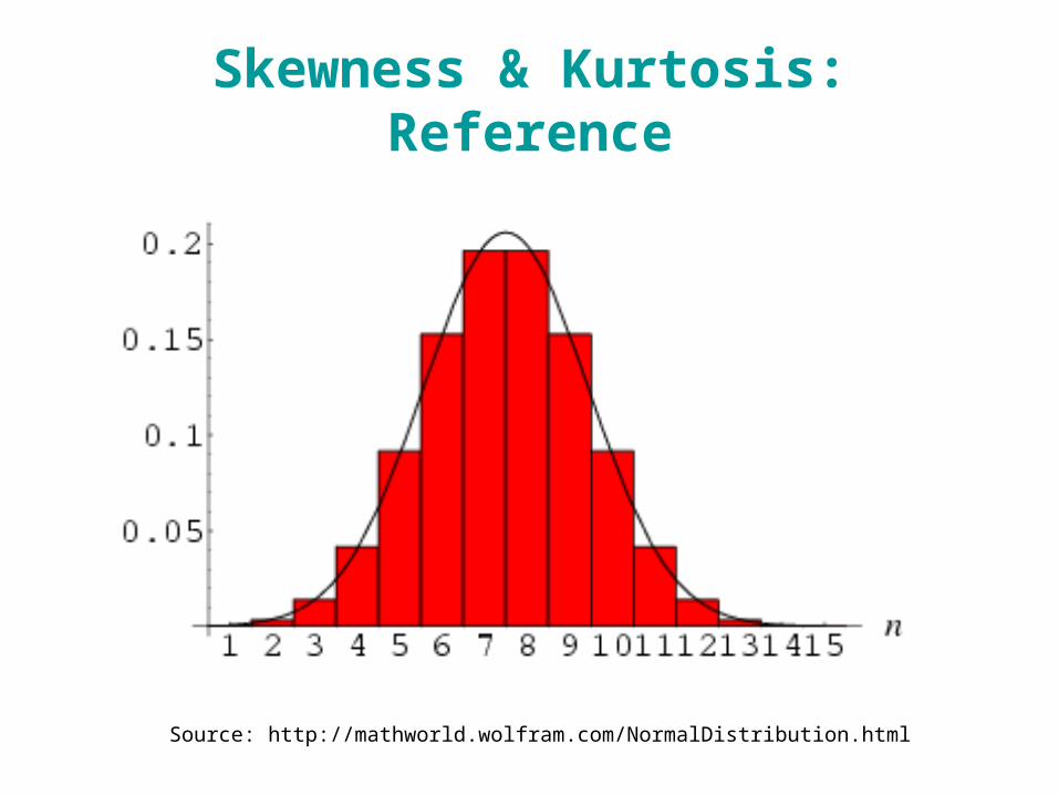
Skewness & Kurtosis: Reference

Source: http://mathworld.wolfram.com/NormalDistribution.html

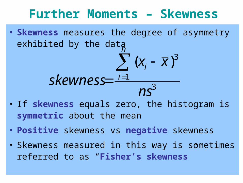
• Skewness measures the degree of asymmetry exhibited by the data

• If skewness equals zero, the histogram is symmetric about the mean

• Positive skewness vs negative skewness

• Skewness measured in this way is sometimes referred to as “Fisher’s skewness”

Further Moments – Skewness

31

3)(

ns

xxskewness

n

ii

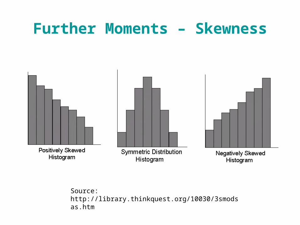
Further Moments – Skewness

Source: http://library.thinkquest.org/10030/3smodsas.htm

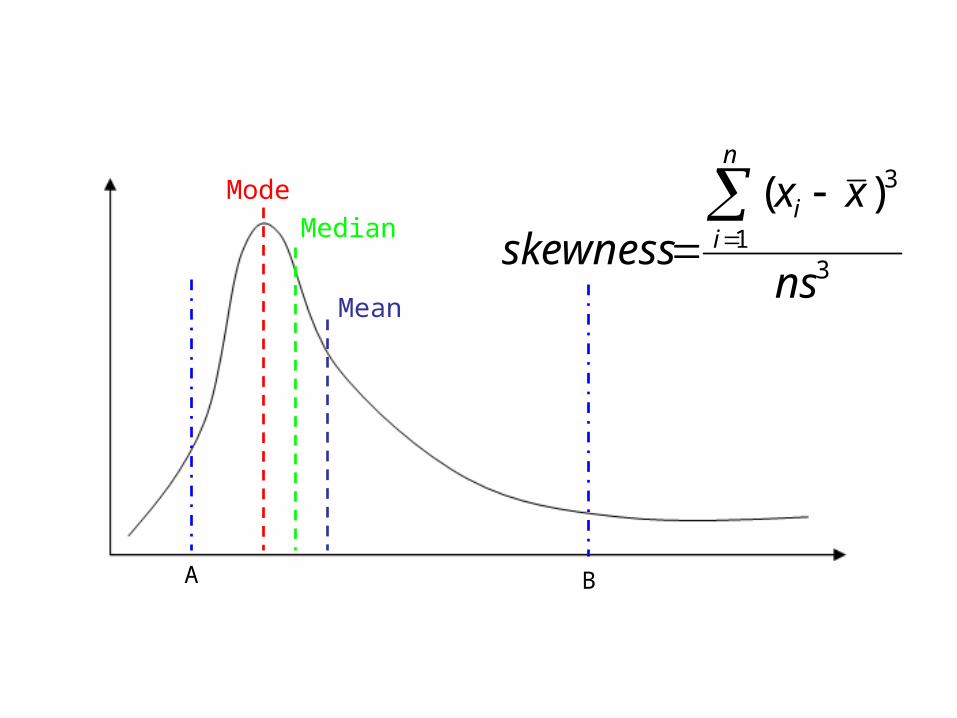
Mode

Median

Mean

31

3)(

ns

xxskewness

n

ii

A B

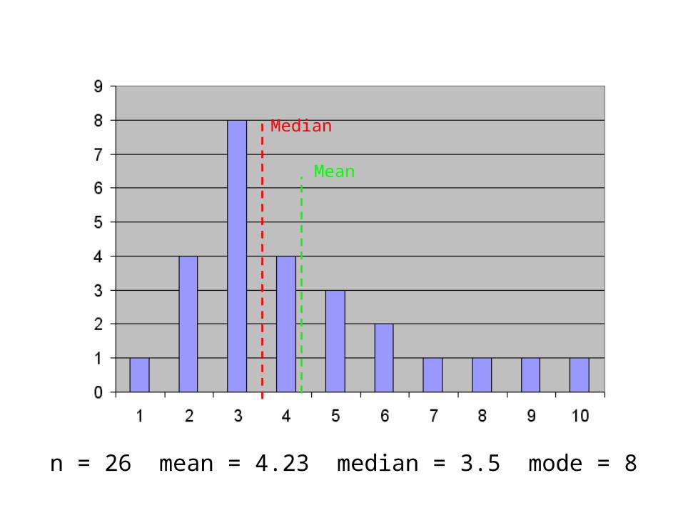
n = 26 mean = 4.23 median = 3.5 mode = 8

Median

Mean

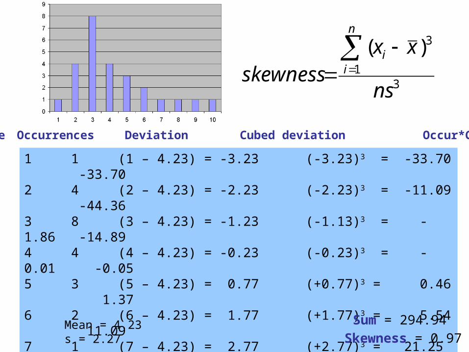
1 1 (1 – 4.23) = -3.23 (-3.23)3 = -33.70 -33.702 4 (2 – 4.23) = -2.23 (-2.23)3 = -11.09 -44.363 8 (3 – 4.23) = -1.23 (-1.13)3 = -1.86 -14.894 4 (4 – 4.23) = -0.23 (-0.23)3 = -0.01 -0.055 3 (5 – 4.23) = 0.77 (+0.77)3 = 0.46 1.376 2 (6 – 4.23) = 1.77 (+1.77)3 = 5.54 11.097 1 (7 – 4.23) = 2.77 (+2.77)3 = 21.25 21.258 1 (8 – 4.23) = 3.77 (+3.77)3 = 53.58 53.589 1 (9 – 4.23) = 4.77 (+4.77)3 = 108.53 108.5310 1 (10 - 4.23)= 5.77 (+5.77)3 = 192.10 192.10

31

3)(

ns

xxskewness

n

ii

Value Occurrences Deviation Cubed deviation Occur*Cubed

Sum = 294.94

Skewness = 0.97Mean = 4.23s = 2.27

Mode

Median

Mean

31

3)(

ns

xxskewness

n

ii

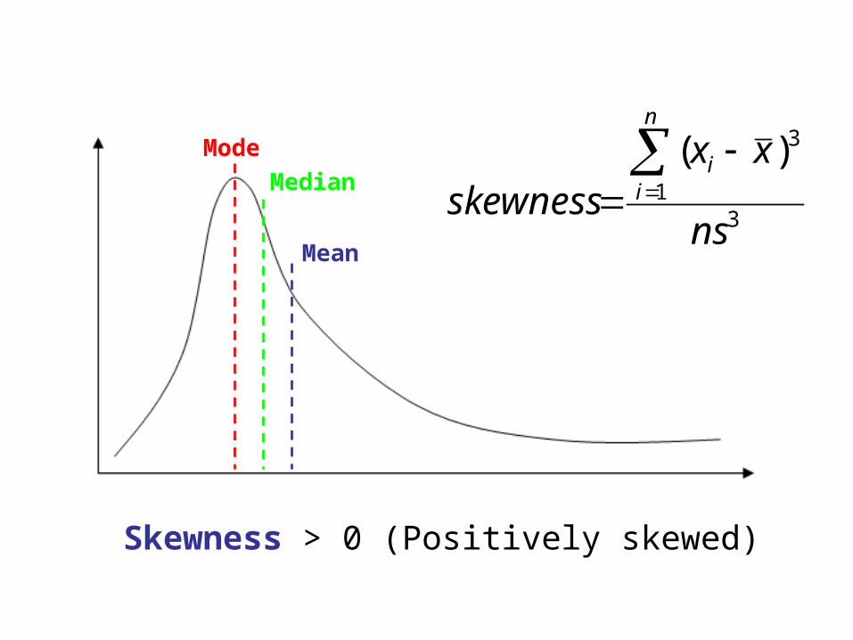
Skewness > 0 (Positively skewed)

Mode

Median

Mean

31

3)(

ns

xxskewness

n

ii

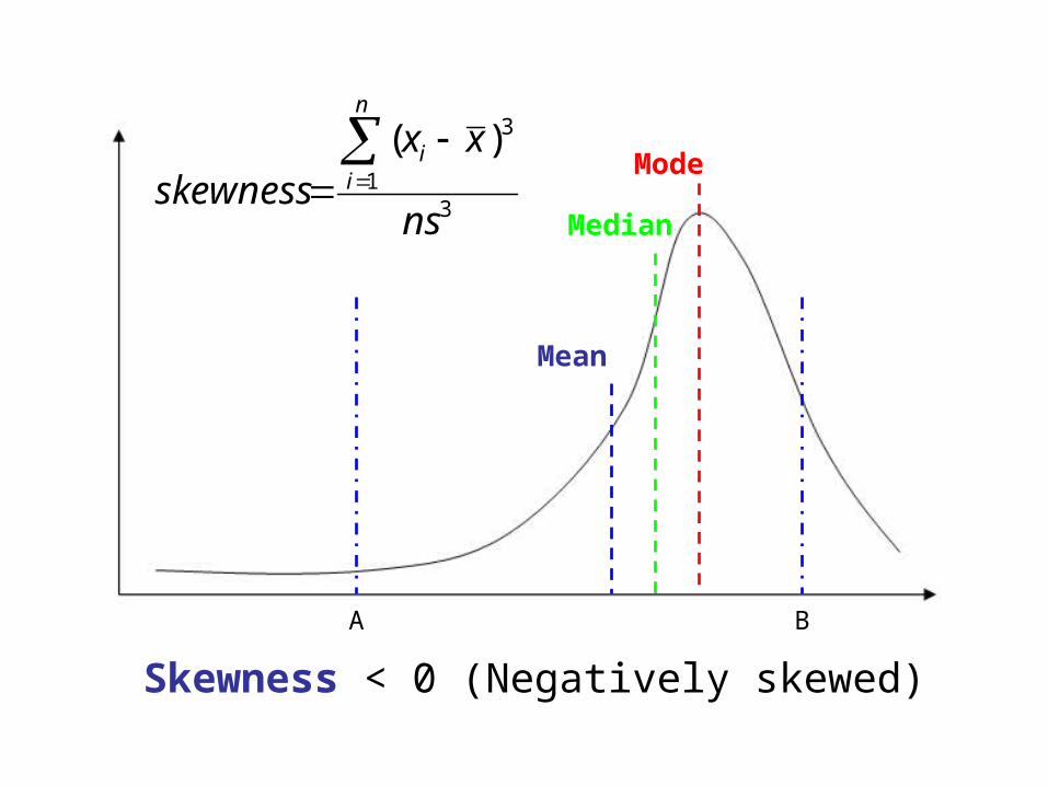
Skewness < 0 (Negatively skewed)

A B

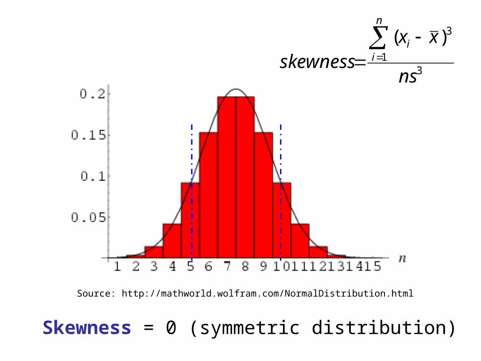
Source: http://mathworld.wolfram.com/NormalDistribution.html

31

3)(

ns

xxskewness

n

ii

Skewness = 0 (symmetric distribution)

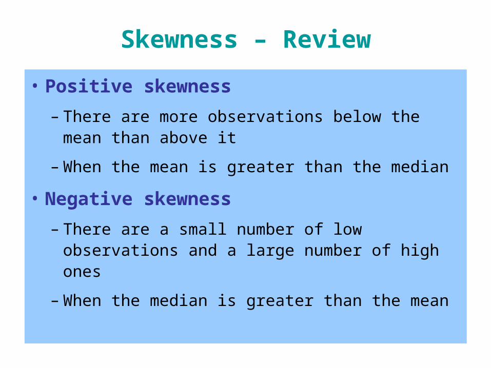
• Positive skewness

– There are more observations below the mean than above it

– When the mean is greater than the median

• Negative skewness

– There are a small number of low observations and a large number of high ones

– When the median is greater than the mean

Skewness – Review

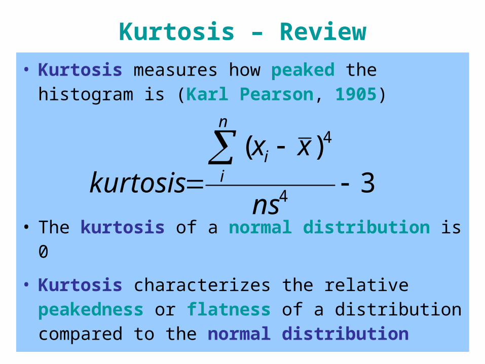
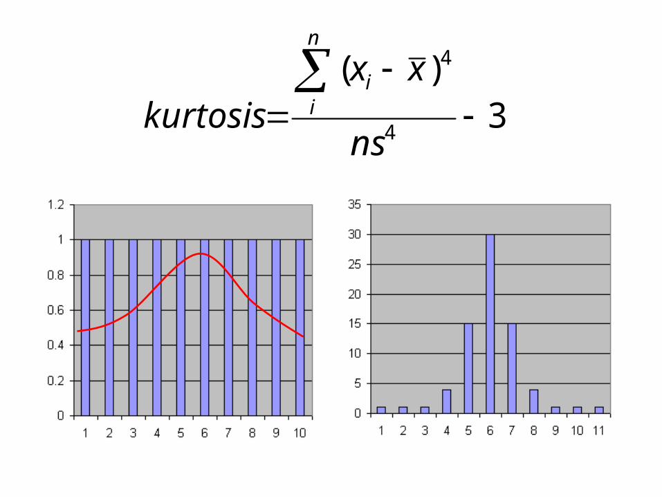
Kurtosis – Review

• Kurtosis measures how peaked the histogram is (Karl Pearson, 1905)

• The kurtosis of a normal distribution is 0

• Kurtosis characterizes the relative peakedness or flatness of a distribution compared to the normal distribution

3)(

4

4

ns

xxkurtosis

n

ii

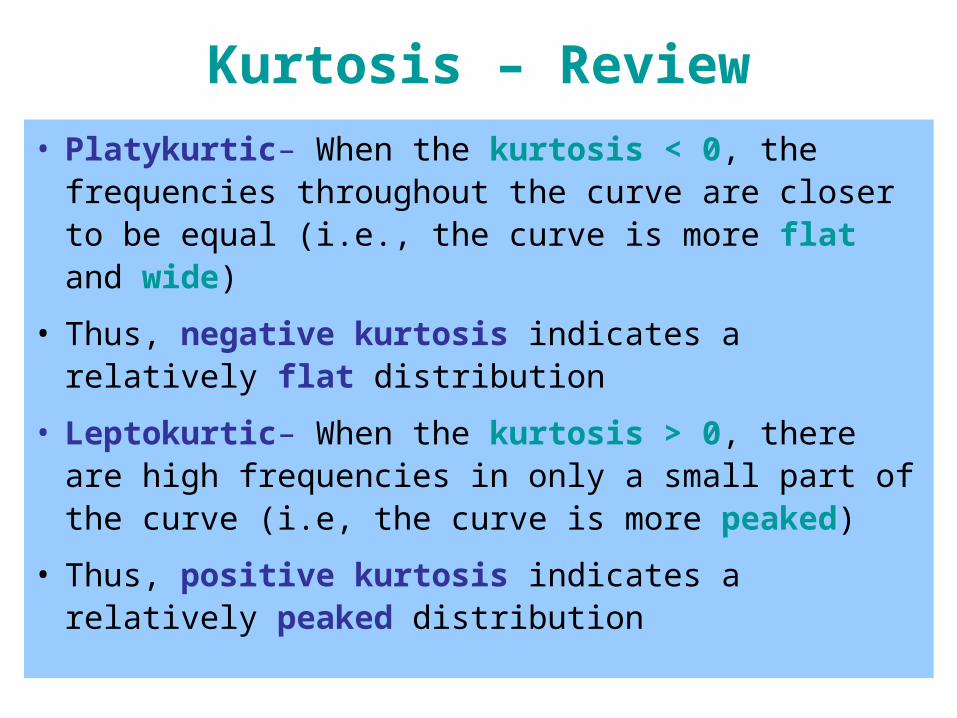
Kurtosis – Review

• Platykurtic– When the kurtosis < 0, the frequencies throughout the curve are closer to be equal (i.e., the curve is more flat and wide)

• Thus, negative kurtosis indicates a relatively flat distribution

• Leptokurtic– When the kurtosis > 0, there are high frequencies in only a small part of the curve (i.e, the curve is more peaked)

• Thus, positive kurtosis indicates a relatively peaked distribution

3)(

4

4

ns

xxkurtosis

n

ii

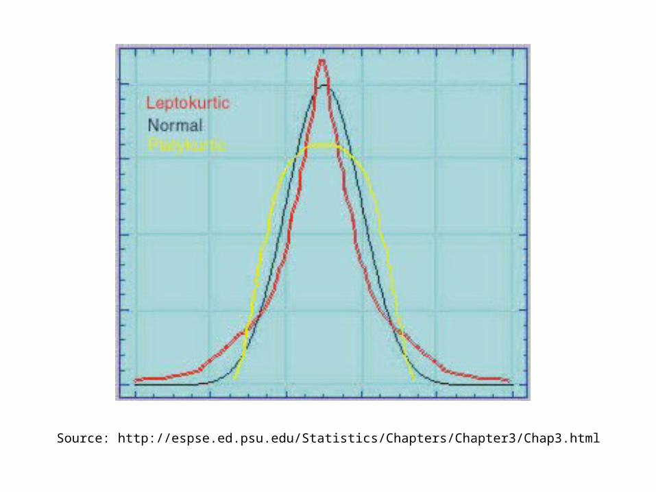
Source: http://espse.ed.psu.edu/Statistics/Chapters/Chapter3/Chap3.html

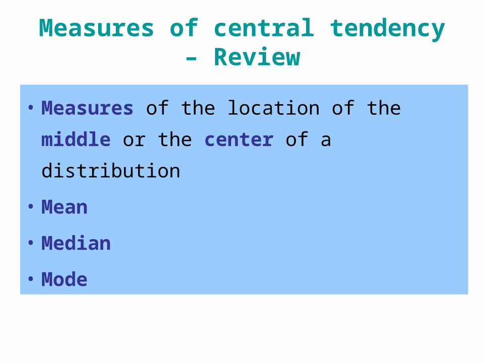
Measures of central tendency – Review

• Measures of the location of the middle or

the center of a distribution

• Mean

• Median

• Mode

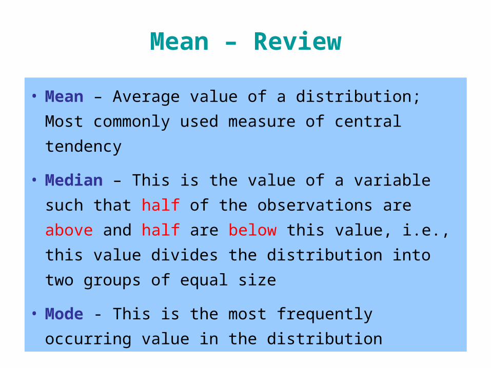
• Mean – Average value of a distribution; Most

commonly used measure of central tendency

• Median – This is the value of a variable such

that half of the observations are above and half

are below this value, i.e., this value divides the

distribution into two groups of equal size

• Mode - This is the most frequently occurring

value in the distribution

Mean – Review

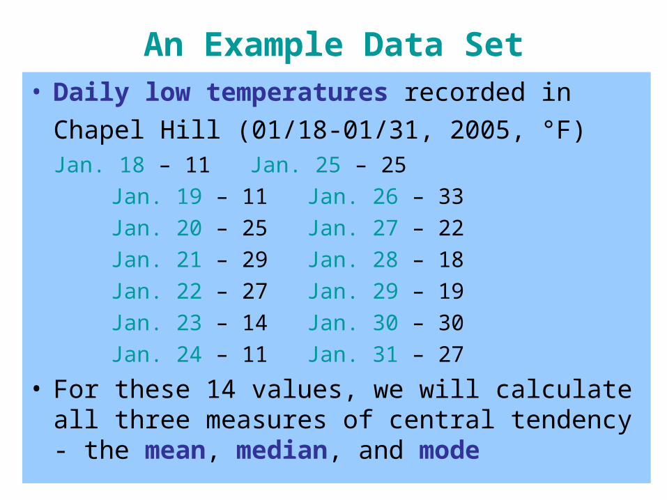
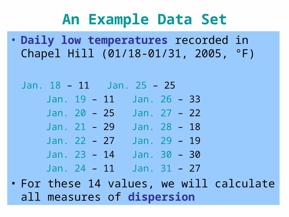
An Example Data Set• Daily low temperatures recorded in Chapel Hill

(01/18-01/31, 2005, °F) Jan. 18 – 11 Jan. 25 – 25

Jan. 19 – 11 Jan. 26 – 33

Jan. 20 – 25 Jan. 27 – 22

Jan. 21 – 29 Jan. 28 – 18

Jan. 22 – 27 Jan. 29 – 19

Jan. 23 – 14 Jan. 30 – 30

Jan. 24 – 11 Jan. 31 – 27

• For these 14 values, we will calculate all three measures of central tendency - the mean, median, and mode

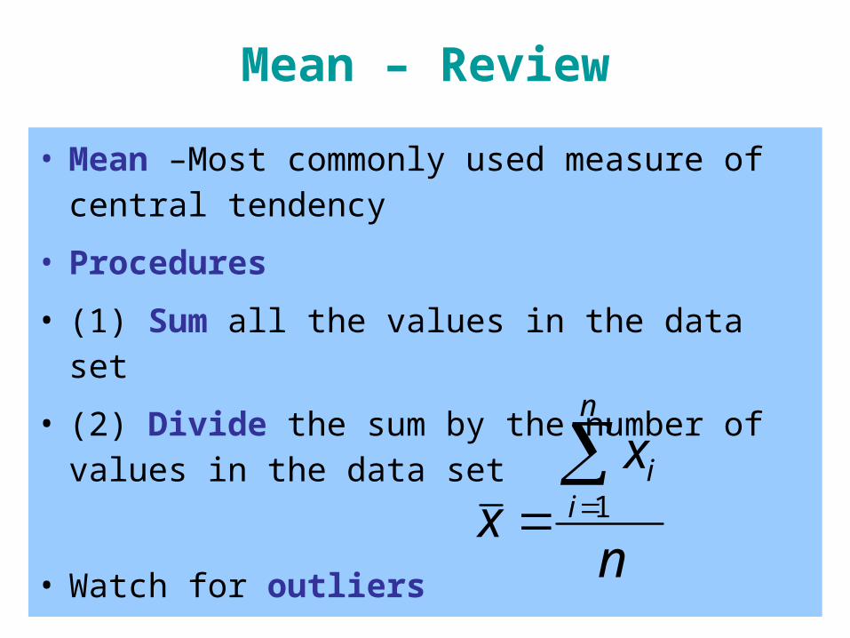
• Mean –Most commonly used measure of central tendency

• Procedures

• (1) Sum all the values in the data set

• (2) Divide the sum by the number of values in the data set

• Watch for outliers n

xx

n

ii

1

Mean – Review

Mean – Review

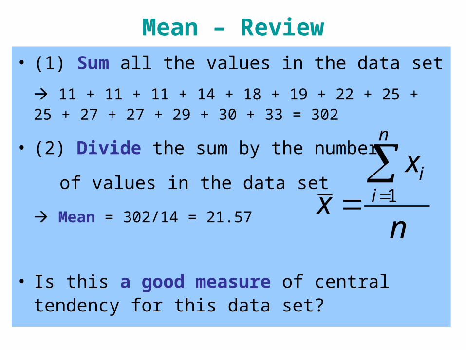
• (1) Sum all the values in the data set

11 + 11 + 11 + 14 + 18 + 19 + 22 + 25 + 25 + 27 + 27 + 29 + 30 + 33 = 302

• (2) Divide the sum by the number

of values in the data set

Mean = 302/14 = 21.57

• Is this a good measure of central tendency for this data set?

n

xx

n

ii

1

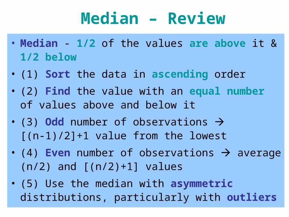
Median – Review

• Median - 1/2 of the values are above it & 1/2 below

• (1) Sort the data in ascending order

• (2) Find the value with an equal number of values above and below it

• (3) Odd number of observations [(n-1)/2]+1 value from the lowest

• (4) Even number of observations average (n/2) and [(n/2)+1] values

• (5) Use the median with asymmetric distributions, particularly with outliers

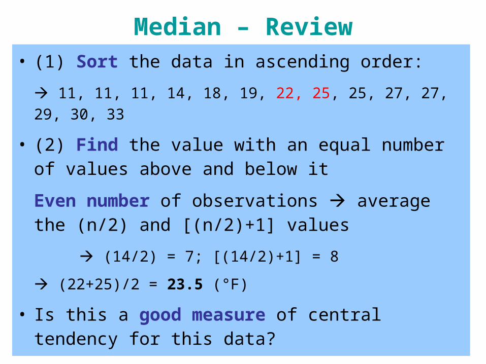
Median – Review• (1) Sort the data in ascending order:

11, 11, 11, 14, 18, 19, 22, 25, 25, 27, 27, 29, 30, 33

• (2) Find the value with an equal number of values above and below it

Even number of observations average the (n/2) and [(n/2)+1] values

(14/2) = 7; [(14/2)+1] = 8

(22+25)/2 = 23.5 (°F)

• Is this a good measure of central tendency for this data?

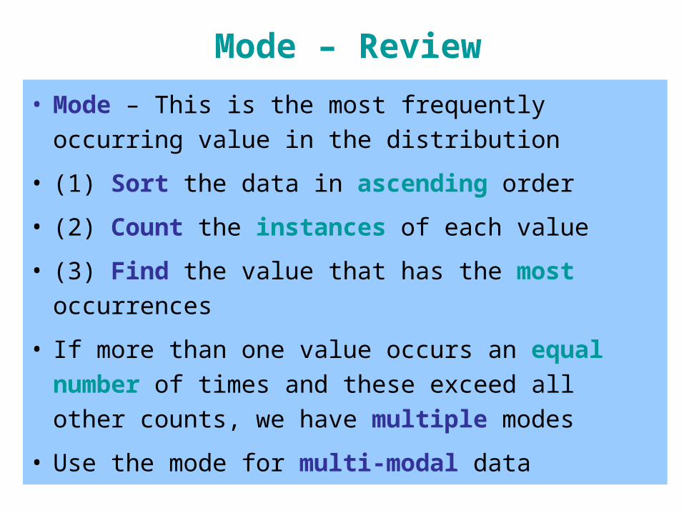
Mode – Review

• Mode – This is the most frequently occurring value

in the distribution

• (1) Sort the data in ascending order

• (2) Count the instances of each value

• (3) Find the value that has the most occurrences

• If more than one value occurs an equal number of

times and these exceed all other counts, we have

multiple modes

• Use the mode for multi-modal data

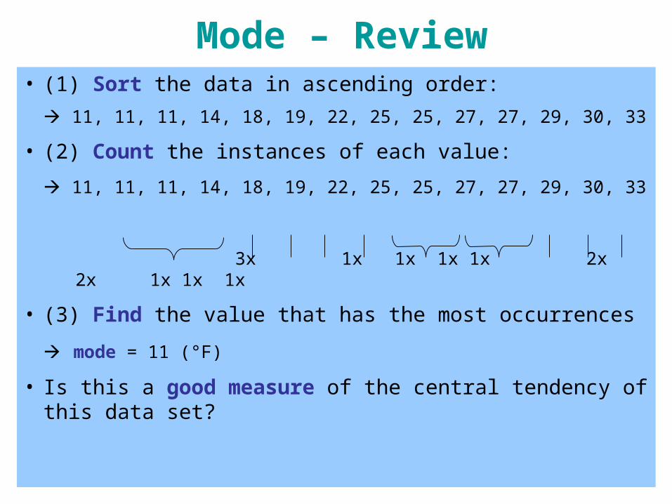
Mode – Review• (1) Sort the data in ascending order:

11, 11, 11, 14, 18, 19, 22, 25, 25, 27, 27, 29, 30, 33

• (2) Count the instances of each value:

11, 11, 11, 14, 18, 19, 22, 25, 25, 27, 27, 29, 30, 33

3x 1x 1x 1x 1x 2x 2x 1x 1x 1x

• (3) Find the value that has the most occurrences

mode = 11 (°F)

• Is this a good measure of the central tendency of this data set?

Measures of Dispersion – Review

• In addition to measures of central tendency, we can also summarize data by characterizing its variability

• Measures of dispersion are concerned with the distribution of values around the mean in data:– Range

– Interquartile range

– Variance

– Standard deviation

– z-scores

– Coefficient of Variation (CV)

An Example Data Set• Daily low temperatures recorded in Chapel Hill

(01/18-01/31, 2005, °F) Jan. 18 – 11 Jan. 25 – 25

Jan. 19 – 11 Jan. 26 – 33

Jan. 20 – 25 Jan. 27 – 22

Jan. 21 – 29 Jan. 28 – 18

Jan. 22 – 27 Jan. 29 – 19

Jan. 23 – 14 Jan. 30 – 30

Jan. 24 – 11 Jan. 31 – 27

• For these 14 values, we will calculate all measures of dispersion

Range – Review

• Range – The difference between the largest and the smallest values

• (1) Sort the data in ascending order

• (2) Find the largest value

max

• (3) Find the smallest value

min

• (4) Calculate the range

range = max - min

• Vulnerable to the influence of outliers

Range – Review

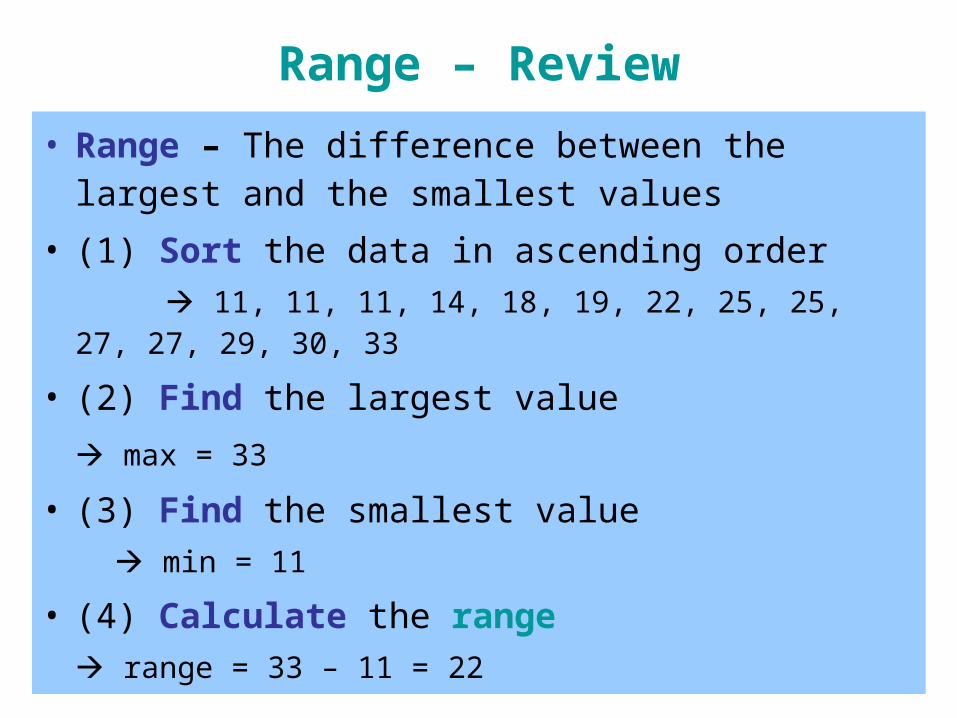
• Range – The difference between the largest and the smallest values

• (1) Sort the data in ascending order

11, 11, 11, 14, 18, 19, 22, 25, 25, 27, 27, 29, 30, 33

• (2) Find the largest value

max = 33

• (3) Find the smallest value

min = 11

• (4) Calculate the range

range = 33 – 11 = 22

Interquartile Range – Review

• Interquartile range – The difference between the

25th and 75th percentiles

• (1) Sort the data in ascending order

• (2) Find the 25th percentile – (n+1)/4 observation

• (3) Find the 75th percentile – 3(n+1)/4 observation

• (4) Interquartile range is the difference between

these two percentiles

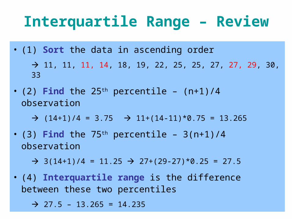
Interquartile Range – Review

• (1) Sort the data in ascending order

11, 11, 11, 14, 18, 19, 22, 25, 25, 27, 27, 29, 30, 33

• (2) Find the 25th percentile – (n+1)/4 observation

(14+1)/4 = 3.75 11+(14-11)*0.75 = 13.265

• (3) Find the 75th percentile – 3(n+1)/4 observation

3(14+1)/4 = 11.25 27+(29-27)*0.25 = 27.5

• (4) Interquartile range is the difference between these two percentiles

27.5 – 13.265 = 14.235

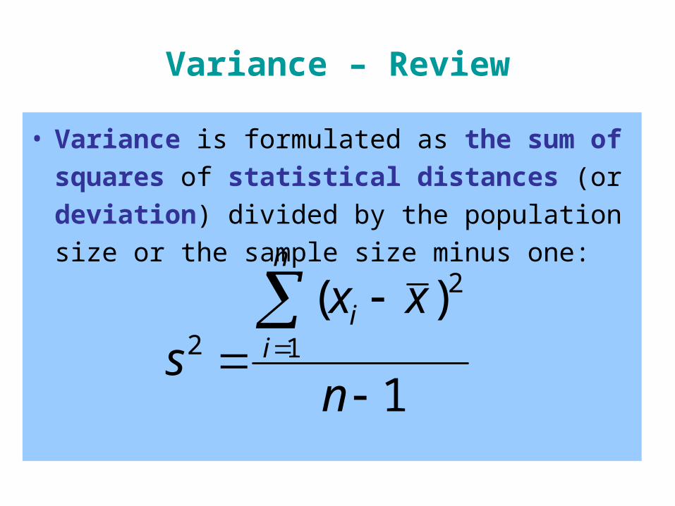
Variance – Review

• Variance is formulated as the sum of squares of

statistical distances (or deviation) divided by

the population size or the sample size minus one:

1

)(1

2

2

n

xxs

n

ii

Variance – Review• (1) Calculate the mean

• (2) Calculate the deviation for each value

• (3) Square each of the deviations

• (4) Sum the squared deviations

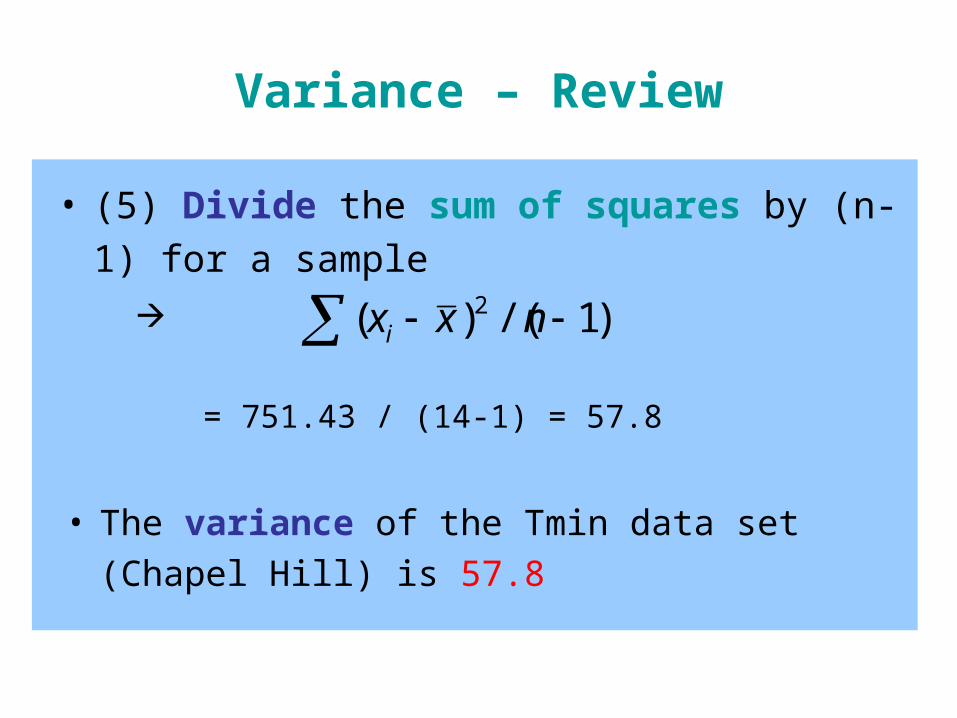
• (5) Divide the sum of squares by (n-1) for a sample

x

xxi

2)( xxi

2)( xxi

)1/()( 2 nxxi

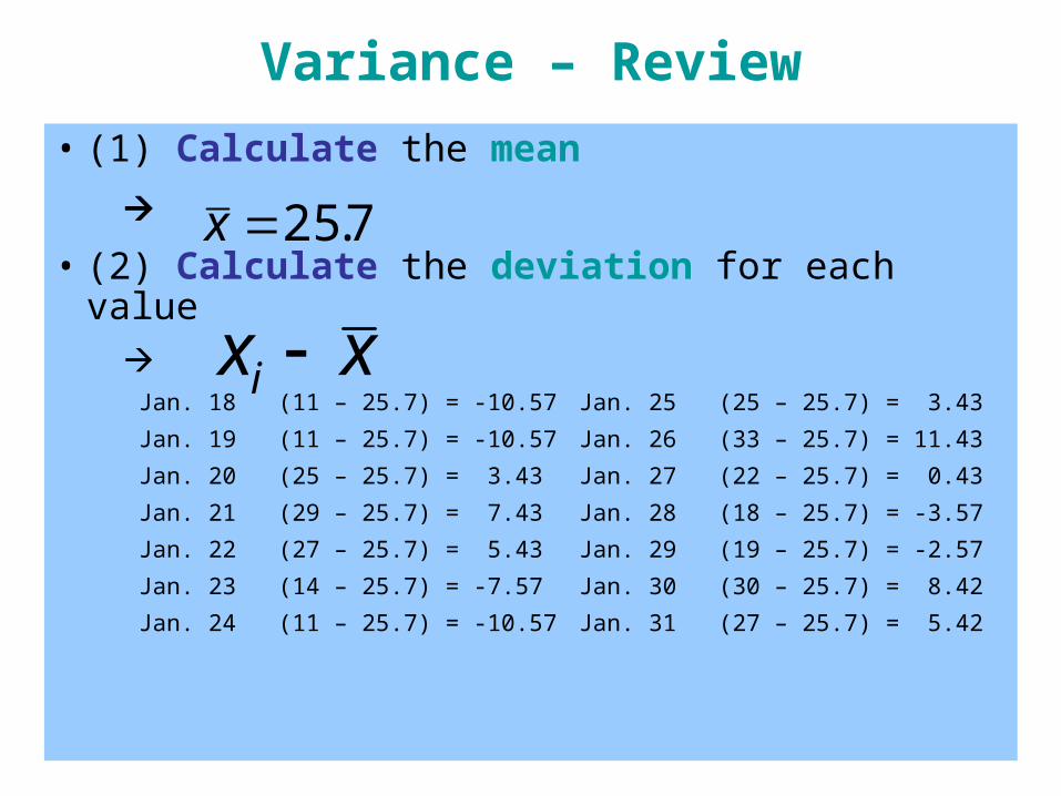
Variance – Review

• (1) Calculate the mean

• (2) Calculate the deviation for each value

Jan. 18 (11 – 25.7) = -10.57 Jan. 25 (25 – 25.7) = 3.43

Jan. 19 (11 – 25.7) = -10.57 Jan. 26 (33 – 25.7) = 11.43

Jan. 20 (25 – 25.7) = 3.43 Jan. 27 (22 – 25.7) = 0.43

Jan. 21 (29 – 25.7) = 7.43 Jan. 28 (18 – 25.7) = -3.57

Jan. 22 (27 – 25.7) = 5.43 Jan. 29 (19 – 25.7) = -2.57

Jan. 23 (14 – 25.7) = -7.57 Jan. 30 (30 – 25.7) = 8.42

Jan. 24 (11 – 25.7) = -10.57 Jan. 31 (27 – 25.7) = 5.42

7.25x

xxi

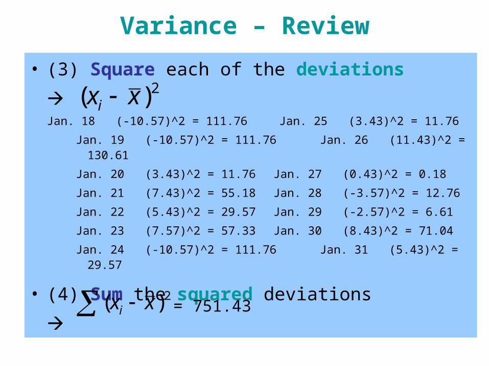
Variance – Review

• (3) Square each of the deviations

Jan. 18 (-10.57)^2 = 111.76 Jan. 25 (3.43)^2 = 11.76

Jan. 19 (-10.57)^2 = 111.76 Jan. 26 (11.43)^2 = 130.61

Jan. 20 (3.43)^2 = 11.76 Jan. 27 (0.43)^2 = 0.18

Jan. 21 (7.43)^2 = 55.18 Jan. 28 (-3.57)^2 = 12.76

Jan. 22 (5.43)^2 = 29.57 Jan. 29 (-2.57)^2 = 6.61

Jan. 23 (7.57)^2 = 57.33 Jan. 30 (8.43)^2 = 71.04

Jan. 24 (-10.57)^2 = 111.76 Jan. 31 (5.43)^2 = 29.57

• (4) Sum the squared deviations

2)( xxi = 751.43

2)( xxi

Variance – Review

• (5) Divide the sum of squares by (n-1) for a

sample

)1/()( 2 nxxi

= 751.43 / (14-1) = 57.8

• The variance of the Tmin data set (Chapel Hill) is

57.8

Standard Deviation – Review

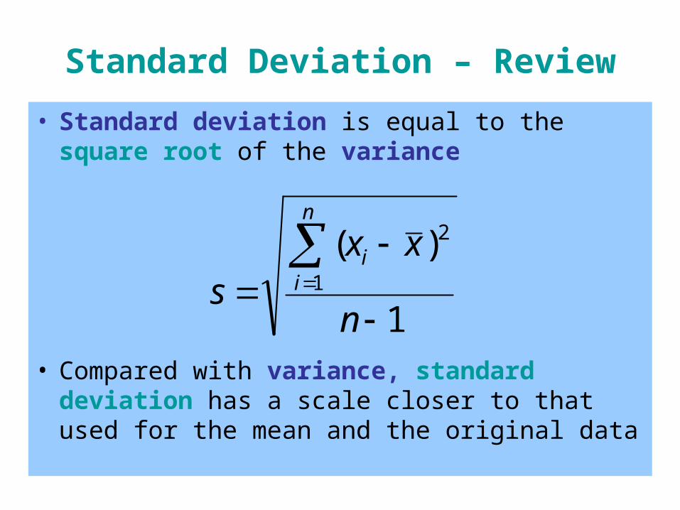
• Standard deviation is equal to the square root of the variance

• Compared with variance, standard deviation has a scale closer to that used for the mean and the original data

1

)(1

2

n

xxs

n

ii

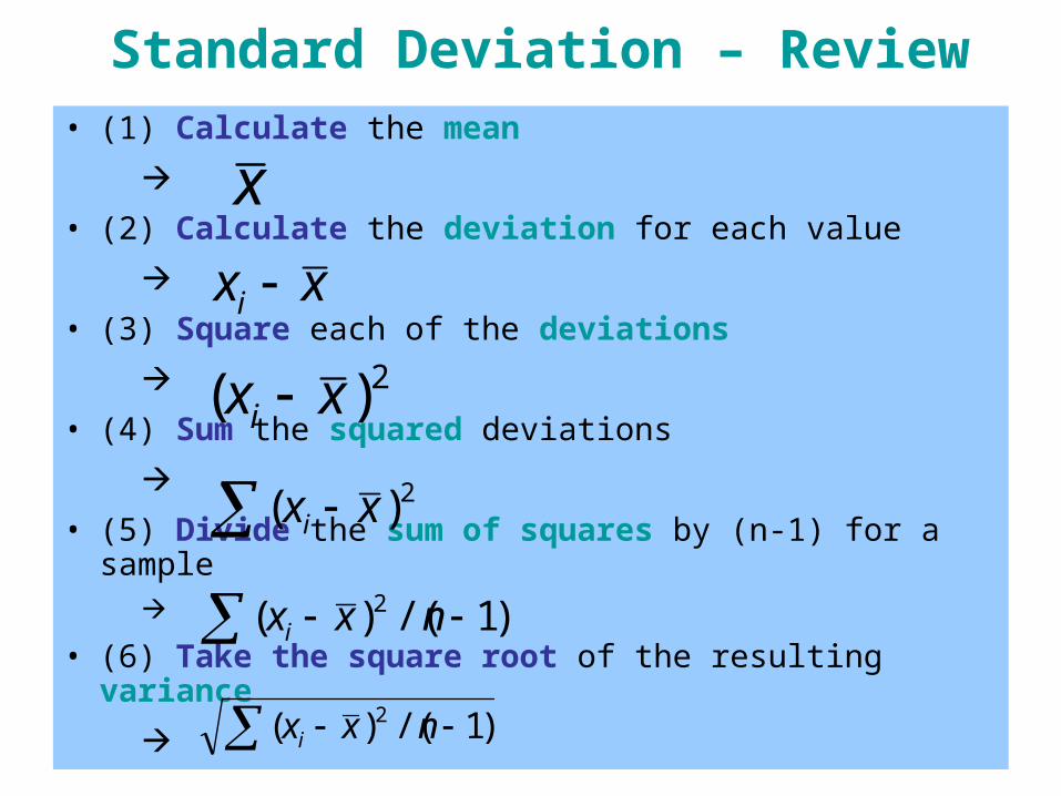
Standard Deviation – Review• (1) Calculate the mean

• (2) Calculate the deviation for each value

• (3) Square each of the deviations

• (4) Sum the squared deviations

• (5) Divide the sum of squares by (n-1) for a sample

• (6) Take the square root of the resulting variance

x

xxi

2)( xxi

2)( xxi

)1/()( 2 nxxi

)1/()( 2 nxxi

Standard Deviation – Review

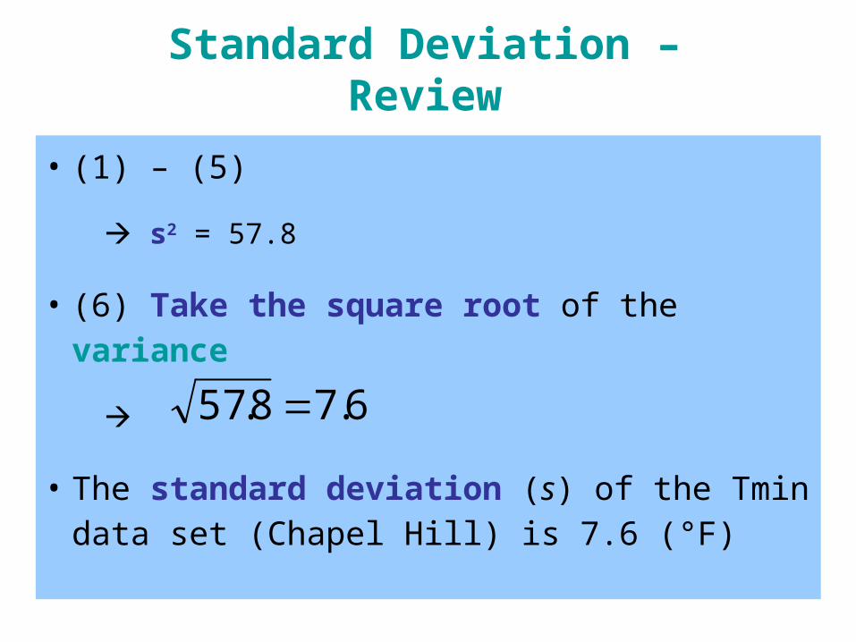
• (1) – (5)

s2 = 57.8

• (6) Take the square root of the variance

• The standard deviation (s) of the Tmin data set (Chapel Hill) is 7.6 (°F)

6.78.57

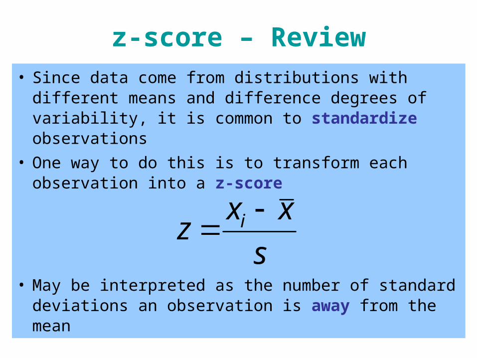
• Since data come from distributions with different means and difference degrees of variability, it is common to standardize observations

• One way to do this is to transform each observation into a z-score

• May be interpreted as the number of standard deviations an observation is away from the mean

s

xxz i

z-score – Review

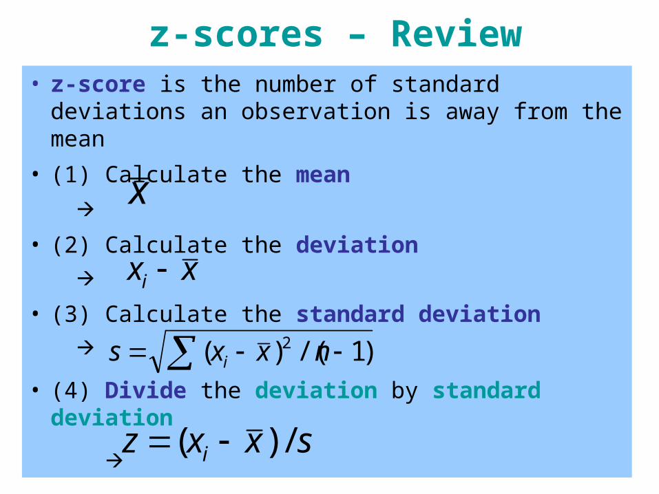
z-scores – Review• z-score is the number of standard deviations an

observation is away from the mean

• (1) Calculate the mean

• (2) Calculate the deviation

• (3) Calculate the standard deviation

• (4) Divide the deviation by standard deviation

)1/()( 2 nxxs i

x

xxi

sxxz i /)(

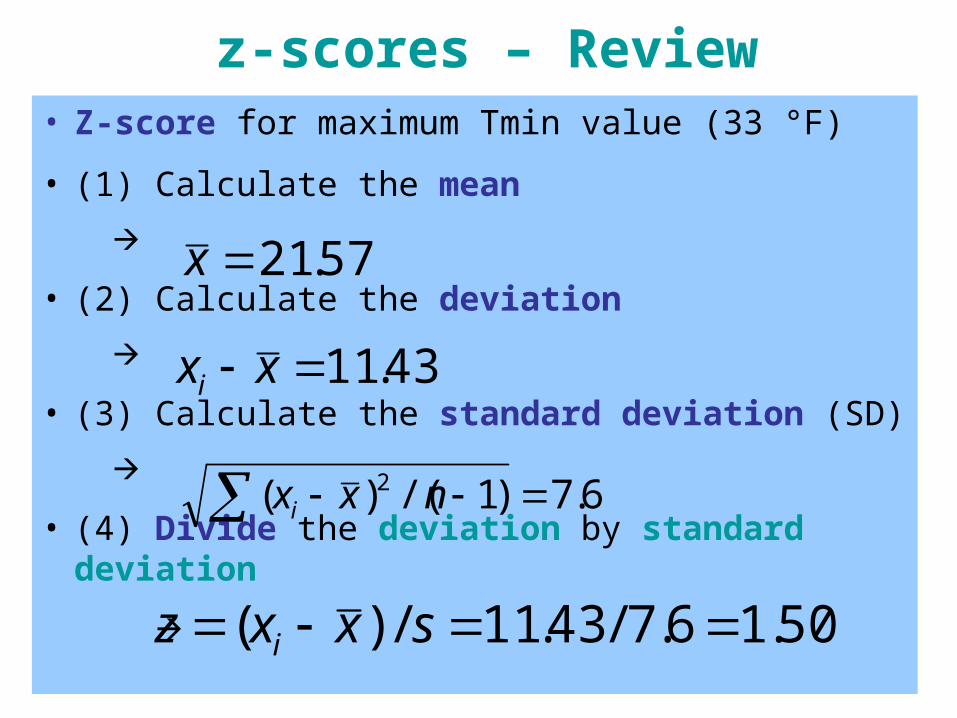
z-scores – Review• Z-score for maximum Tmin value (33 °F)

• (1) Calculate the mean

• (2) Calculate the deviation

• (3) Calculate the standard deviation (SD)

• (4) Divide the deviation by standard deviation

6.7)1/()( 2 nxxi

57.21x

43.11 xxi

50.16.7/43.11/)( sxxz i

Coefficient of Variation – Review

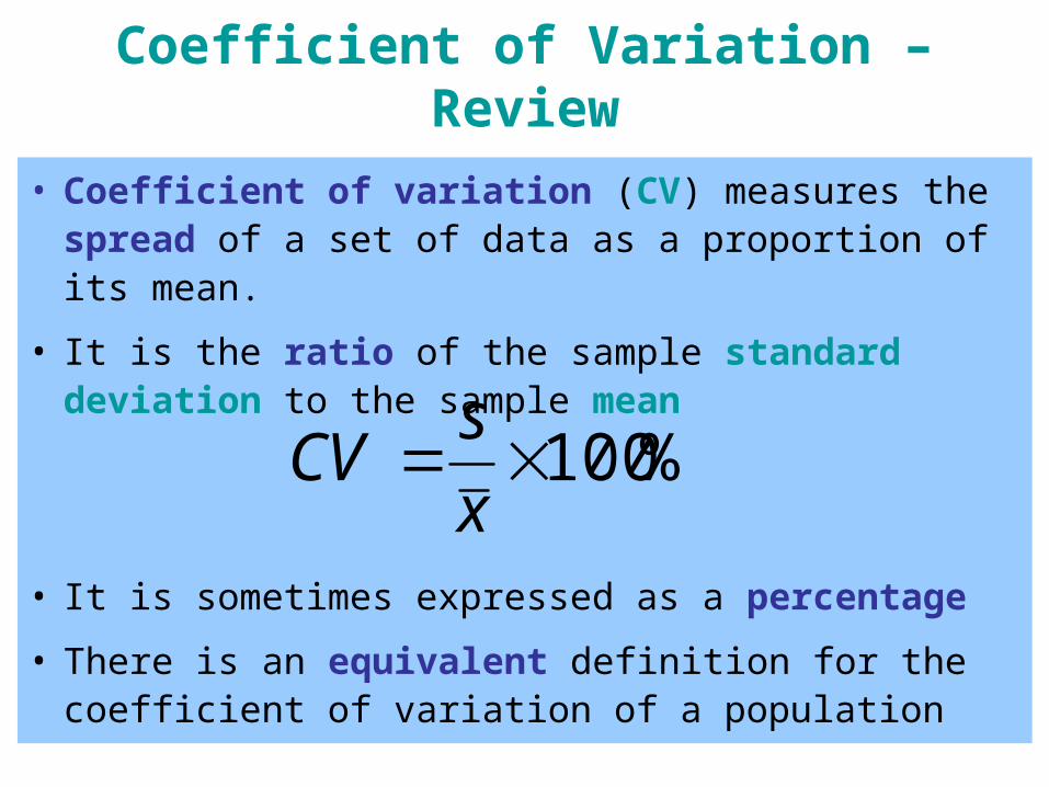
• Coefficient of variation (CV) measures the spread of a set of data as a proportion of its mean.

• It is the ratio of the sample standard deviation to the sample mean

• It is sometimes expressed as a percentage

• There is an equivalent definition for the coefficient of variation of a population

%100x

sCV

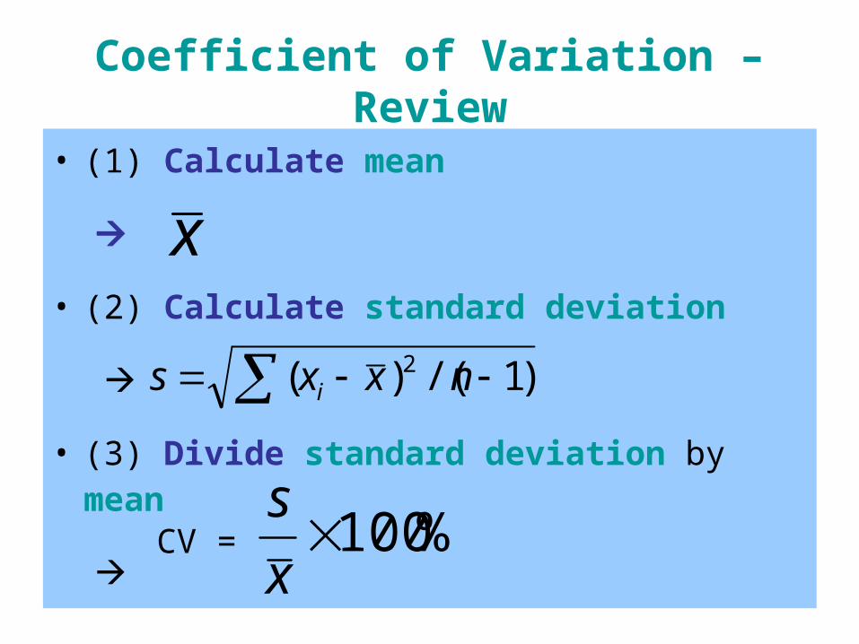
Coefficient of Variation – Review

• (1) Calculate mean

• (2) Calculate standard deviation

• (3) Divide standard deviation by mean

%100x

s

x

CV =

)1/()( 2 nxxs i

Coefficient of Variation – Review

• (1) Calculate mean

• (2) Calculate standard deviation

• (3) Divide standard deviation by mean

58.29%1007.25/6.7%100 x

s

7.25x

CV =

6.7)1/()( 2 nxxs i

Histograms – Review

• We may also summarize our data by constructing histograms, which are vertical bar graphs

• A histogram is used to graphically summarize the distribution of a data set

• A histogram divides the range of values in a data set into intervals

• Over each interval is placed a bar whose height represents the percentage of data values in the interval.

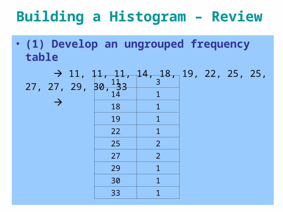
Building a Histogram – Review

• (1) Develop an ungrouped frequency table

11, 11, 11, 14, 18, 19, 22, 25, 25, 27, 27, 29, 30,

33

11 3

14 1

18 1

19 1

22 1

25 2

27 2

29 1

30 1

33 1

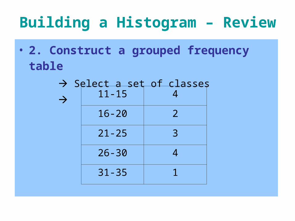
Building a Histogram – Review

• 2. Construct a grouped frequency table

Select a set of classes

11-15 4

16-20 2

21-25 3

26-30 4

31-35 1

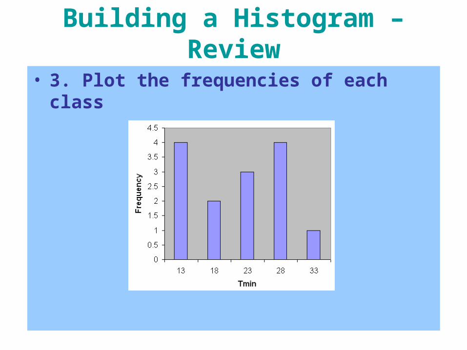
Building a Histogram – Review

• 3. Plot the frequencies of each class

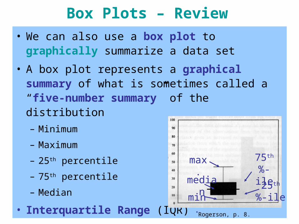
Box Plots – Review

• We can also use a box plot to graphically summarize a data set

• A box plot represents a graphical summary of what is sometimes called a “five-number summary” of the distribution

– Minimum

– Maximum

– 25th percentile

– 75th percentile

– Median

• Interquartile Range (IQR)Rogerson, p. 8.

min.

max.

25th

%-ile

75th

%-ilemedian

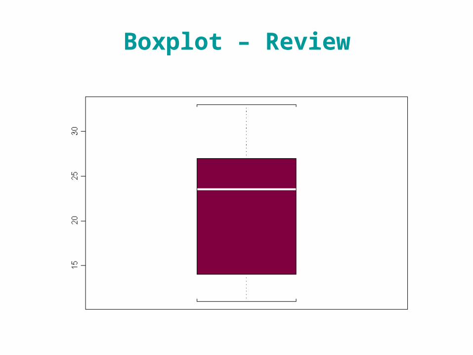
Boxplot – Review

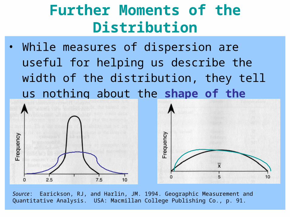
Further Moments of the Distribution

• While measures of dispersion are useful for helping us describe the width of the distribution, they tell us nothing about the shape of the distribution

Source: Earickson, RJ, and Harlin, JM. 1994. Geographic Measurement and Quantitative Analysis. USA: Macmillan College Publishing Co., p. 91.

Skewness – Review

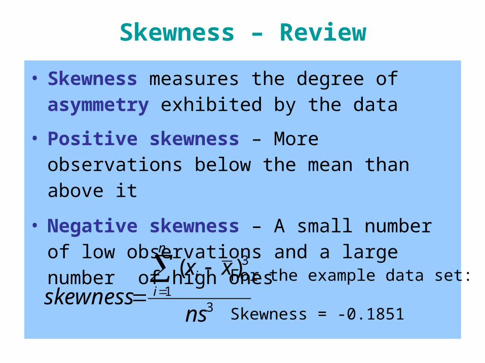
• Skewness measures the degree of asymmetry exhibited by the data

• Positive skewness – More observations below the mean than above it

• Negative skewness – A small number of low observations and a large number of high ones

31

3)(

ns

xxskewness

n

ii

For the example data set:

Skewness = -0.1851

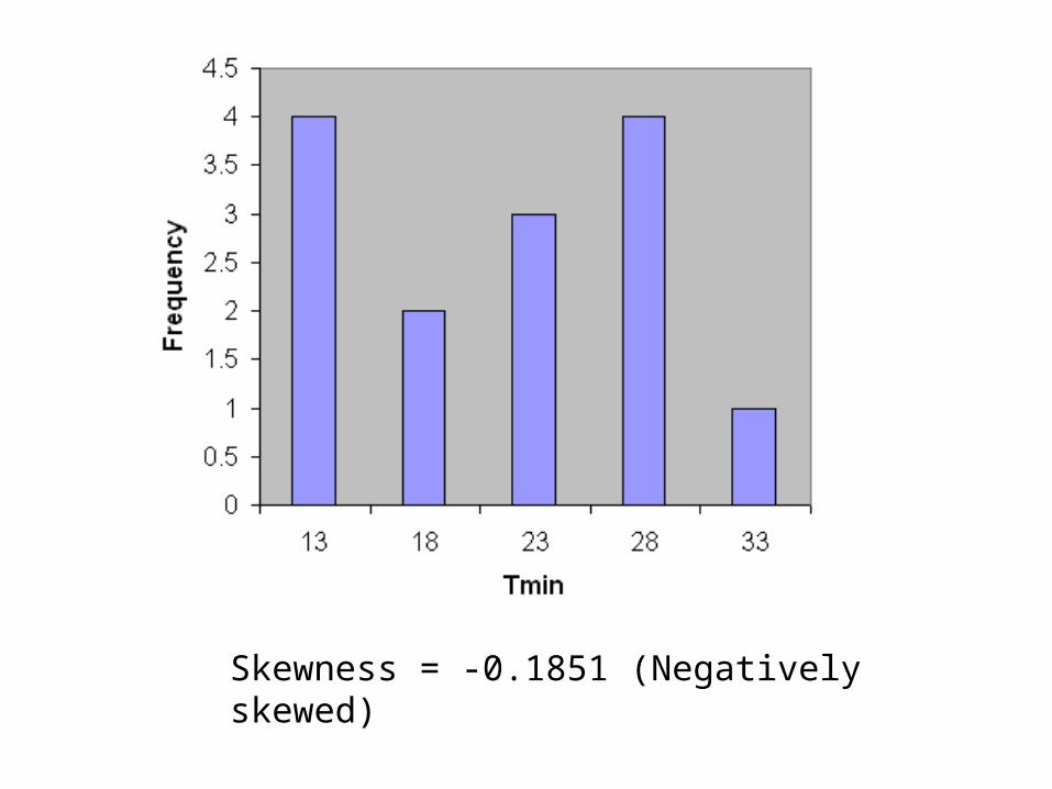
Skewness = -0.1851 (Negatively skewed)

Kurtosis – Review

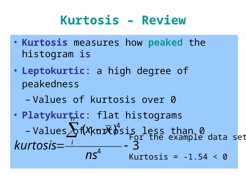
• Kurtosis measures how peaked the histogram is

• Leptokurtic: a high degree of peakedness

– Values of kurtosis over 0

• Platykurtic: flat histograms

– Values of kurtosis less than 0

3)(

4

4

ns

xxkurtosis

n

ii For the example data set:

Kurtosis = -1.54 < 0

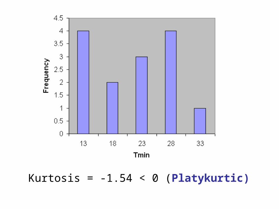
Kurtosis = -1.54 < 0 (Platykurtic)