does industry self-regulation reduce pollution?

1

DOES INDUSTRY SELF-REGULATION REDUCE POLLUTION? RESPONSIBLE CARE IN THE CHEMICAL INDUSTRY

Shanti Gamper-Rabindran

and

Stephen R. Finger

5/7/2012

Journal of Regulatory Economics, forthcoming Shanti Gamper-Rabindran, Assistant Professor, Graduate School of Public and International Affairs, University of Pittsburgh, 3205 Posvar Hall, 230 S. Bouquet St., Pittsburgh PA 15217 ([email protected]) and Stephen R. Finger, Assistant Professor, Moore School of Business, University of South Carolina, 1705 College Street, Columbia, SC 29208 ([email protected]). Corresponding author: Gamper-Rabindran. We thank participants at the California Workshop in Environmental Economics, the European Union Corporate Social Responsibility workshop, World Congress for Environmental and Resource Economics, Association of Public Policy and Management, Eastern Economic Association, and seminars at the University of South Carolina, Carnegie Mellon University and RAND for their helpful comments. Funding from the National Science Foundation BCS 0351058 and the University of Pittsburgh’s Central Research Development Fund, Center for Social and Urban Research, Center for Race and Social Problems and the European Union Center, is gratefully acknowledged. Errors are ours.

2

Abstract

Self-regulation programs, in which industry associations set membership codes beyond

government regulations, are prevalent despite scarce evidence on their effectiveness. We

examine Responsible Care (RC) in the US chemical manufacturing sub-sector, whose

membership codes include pollution prevention, using our author-constructed panel database of

3,278 plants owned by 1,759 firms between 1988 and 2001. We apply two sets of instrumental

variables to address a plant’s parent firm’s self-selection into the program, using: (i) the

characteristics of other plants belonging to the same firm in our multi-plant sample; and (ii) firm

participation in the industry association before the establishment of RC and industry-level RC

participation in our full sample. We find that on average, plants owned by RC participating firms

raise their toxicity-weighted pollution by 15.9% relative to statistically-equivalent plants owned

by non-RC participating firms. This estimated increase is large relative to the yearly 4%

reduction in pollution among all plants in our sample between 1988 and 2001. Moreover, RC

raises plant-level pollution intensity by 15.1%. These results caution against reliance on self-

regulation programs modeled on the pre-2002 RC program that did not require third party

certification and in those sectors that lack independent third party certification.

JEL codes : Q53 Q58 L51 L65 D21 Keywords: Corporate Social Responsibility, self-regulation, voluntary programs, self-selection, greenwash, chemical industry

3

1. Industry Self-Regulation: Responsible Care

Self-regulation programs, in which industry associations set codes of conduct for their

members against the backdrop of government regulations, are prominent even in the high risk

chemical and nuclear sectors (NCBP, 2011). One major justification for relying on industry self-

regulation to manage environmental risks is that firms have more information, expertise and

resources than government regulators (National Academy of Engineering, 2010; GAO, 2011).

The most prominent of these programs is Responsible Care in the chemical sector. The American

Chemistry Council (ACC), that sector’s trade association, mandates its members to join the self-

regulation program and adhere to its codes including pollution prevention. The ACC describes

management strategies and provides technical assistance to members in order to implement these

codes (ACC, 1990).

We test the impact of Responsible Care (RC) in the US chemical manufacturing sub-

sector1 on plant-level pollution (defined as toxicity-weighted air pollution).2 Our assessment is

timely because high risk sectors are emulating RC, despite limited empirical evidence on its

effectiveness. Most recently, the National Commission on the BP Oil Spill, noting that RC has

improved environmental management in the chemical sub-sector, recommended that the oil and

gas drilling sector create a self-regulation program (NCBP, 2011). In turn, that sector’s industry

association is considering the adoption of a self-regulation program that incorporates features

from RC (Dlouhy, 2011). Yet, the only empirical study on RC (King and Lenox, 2000) reports

that RC participants reduce their pollution at slower rates than non-participants. However, a key

1 The Standard Industrial Classification (SIC) preceded the current North American Industry Classification System. We study the SIC-28 chemical manufacturing major-group. The SIC-28 major group contains industries at the SIC 4-digit level (SIC-4). Our plants are from SIC 2851 - Paints, Varnishes, Lacquers, and Enamels (18%), SIC 2821 - Plastics Materials and Synthetic Resins (11%), SIC 2869 - Industrial Organic Chemicals, not elsewhere classified (11%), and other SIC-4 industries. 2 Most pollution reported to the Toxic Release Inventory is emitted into air (Potoski and Prakash, 2005).

4

drawback in that innovative study is that it does not address firms’ self-selection into the

program, which is likely based on factors that are unobserved by researchers but correlated with

the program outcome (Hartman, 1988; Levinson, 2004). The direction of bias when firms’ self-

selection into RC is not addressed is not known a priori (section 2.3). Therefore, King and Lenox

(2000) may be biased against or towards finding that RC reduces pollution.

Our study applies instrumental variables to address firms’ self-selection into RC. For a

plant belonging to a multi-plant firm, we instrument for the RC participation status of a plant’s

parent firm using characteristics of other plants belonging to the same firm. Factors such as

strong regulatory pressure on these other plants reduce a firm's overall costs of joining RC (the

firm would have to reduce pollution in any case, and it might as well join RC and share the

benefits). However, these regulatory factors at other plants are less likely to directly affect

pollution at a given plant (section 3.5). As imperfect instruments in the full sample, (truly

exogenous instruments for single-plant firms are difficult to identify), we use the share of rival

plants in the given industry participating in RC and the parent firm’s participation in the ACC

before the creation of RC.

We implement a system Generalized Method of Moments (GMM) estimator to our author

constructed panel database of the US chemical manufacturing sector, with 3,278 plants owned by

1,759 firms between 1988 and 2001. We examine RC’s impact on plant-level pollution because

RC’s stated goal is to reduce pollution, and total pollution reduction is relevant for

environmental protection. We find robust evidence that, controlling for self-selection, RC fails to

reduce plant-level pollution. Our preferred estimates, from our multi-plant sample, indicate that

plants owned by RC participating firms raise their pollution by 15.9% relative to statistically-

equivalent plants owned by non-RC participating firms. These estimates are large compared to

5

the yearly 4% reduction in pollution among all plants in our sample between 1988 and 2001,3

i.e., participation in RC eliminates at least 3 years of this trend. Allowing for the possibility of

heterogeneous program effects, we do not find any subsets of plants that reduce their pollution.

Our results are robust to the use of different subsets of instruments and the alternative

measurement of pollution in pounds. We find comparable results that RC raises pollution by

16.1% in our full sample (though we note the limitations in the instruments used in the full

sample). Finally, our estimation using Propensity Score Matching (PSM), a method whose

consistency does not rely on exclusion restrictions, yields estimates that range from one third to

the full magnitude of the GMM estimates (6.8% to 16.8%). However, the PSM estimates are not

statistically significant.4 As a further check, we examine if RC reduces pollution intensity,

defined as the ratio of plants’ toxicity-weighted air pollution to their number of employees.5

Lower pollution intensity would imply a more favorable trade-off between production and

pollution (Cole et al., 2005).6 Instead, we find that RC raises pollution intensity by 15.1% in the

multi-plant sample.7

Our study, consistent with Glachant’s (2007) theory that firms may enter self-regulation

programs without any intention of meeting their program commitments, has important policy

implications. RC has been adopted by chemical associations in 53 countries as of 2008 (ICCA,

2008). Moreover, the pre-2002 RC program shares the two key characteristics of major industry

self-regulation programs, i.e., its absence of third party verification and enforceable penalties for

non-performance. Programs modeled on RC, such as the petroleum industry’s self-regulation

3 The annual decline is 5.8% for RC participants and 4.2% for non-participants between 1988 and 2001. 4 The strengths and weaknesses of the GMM and PSM methods are discussed in section 5.21. 5 For evidence that the number of employees can serve as a proxy for the preferred denominator of output, see Online Appendix III. Plant-level output data is not publicly available. 6 All things equal, with lowered pollution intensity, the same amount of production would result in less pollution (Cole et al., 2005).

6

program (Hoffman, 2000) or programs in which certifiers are not truly independent (O’Rourke,

2003; Rosenthal and Kunreuther, 2010), may not improve environmental performance. Our

results provide timely guidance to regulators and the oil and gas drilling industry, which are

drawing on lessons from RC. Independent third party certification is, in practice, limited in the

oil and gas sector (Bea, pers. comm.; Pettit, 2010).8 Therefore, our result on the ineffectiveness

of the pre-2002 RC program, which does not require third party certification, cautions against

reliance on self-regulation as the primary policy tool for improving environmental performance.9

Section 2 reviews the literature on industry self-regulation and outlines the institutional features

of the RC program. Section 3 describes our estimation strategy. Section 4 describes our data.

Section 5 presents our results, with conclusions and policy implications in Section 6.

2. Industry Self-Regulation and Pollution Reduction

2.1 Can industry self-regulation reduce pollution?

Self-regulation programs limit their membership to firms that commit to their codes of

conduct. Whether these programs, which have limited ability to monitor and sanction their

members, can ensure their members truly undertake risk reduction is under debate (Kleindorfer

and Orts, 1998; Lyon and Maxwell, 2004; Barnett and King, 2008). The industry faces strong

incentives to create a credible self-regulation program that reduces pollution if the program could

forestall the state’s imposition of stricter and more costly regulation (Maxwell et al., 2000).

Importantly, Dawson and Segerson’s (2008) theoretical study shows that even if other firms were

7 The estimate is 12.6% in the full sample, in which our instruments are imperfect. 8 Certifiers, which rely exclusively on clientele from that sector, face economic pressure to provide positive assessments (Bea, pers. comm; Pettit, 2010). Robert Bea, email message to Shanti Gamper-Rabindran on 07/06/2011. Bea is with the Deepwater Horizon Study Group (distinct from NCBP), Center for Catastrophic Risk Management, University of California, Berkeley, Professor Emeritus in Engineering, 9 Cohen et al. (2011) explore alternative policies to improve environmental performance in the oil and gas drilling sector.

7

to free-ride, a critical number of firms will reduce their pollution in order to maintain the overall

credibility of the self-regulation program.10

However, skeptics argue that self-regulation programs can serve as ‘greenwash,’ i.e.,

firms join these programs to signal green, but fail to reduce their adverse environmental impacts

(Lyon and Maxwell, 2011). In other words, firms purport to meet their program commitments

without addressing the underlying environmental concerns (Calcott, 2010). Glachant (2007),

noting that his theory applies to self-regulation programs such as RC, argues that firms may or

may not reduce their pollution in response to their participation in self-regulation programs.

Under specific circumstances, “firms may enter strategically into [self-regulation programs]

without any willingness to comply, simply to postpone legislative intervention” (Glachant,

2007). In his model, firms’ non-compliance with their commitments to the self-regulation

program is not observed immediately by the regulator and thus, firms are able to lobby congress

to influence the stringency of the final legislation. Despite the possibility that firms may fail to

comply with their commitments, the regulator agrees to the self-regulation program. The

regulator postpones presenting its legislative proposal to congress until after it has had the

opportunity to observe these firms’ performance. The regulator chooses this course of action

because a self-regulation program in which firms choose to comply with their commitments

would achieve greater pollution reduction than the final legislation weakened by lobbying

efforts.

2.2 Responsible Care: institutional structure

10 Participants also benefit from their positive reputation in their interactions with consumers and investors (Maxwell and Decker, 2006). Participation may reduce inspections by regulatory agencies (Maxwell and Decker, 2006; Innes and Sam, 2008) and discourage boycotts by environmental groups or pre-empt their lobbying for stricter regulations (Baron, 2001; Maxwell et al., 2000).

8

In response to the Bhopal accident, the ACC executive committee reported to its

members that the public deeply distrusted the chemical sector and that the industry needed “to

improve its performance -- not just its image -- in a way the public can see and appreciate”

(Rees, 1997). Subsequently, in September 1988, the ACC adopted the RC program and

mandated its members’ participation in the program (Rees, 1997). In the next five years, ACC’s

technical experts developed six Codes of Management Practices for the industry (Rees, 1997).

Several features of the RC program can potentially lead to pollution reduction. First, RC

requires firms to commit to the Code of Pollution Prevention.11 The ACC exercises some

oversight on firms by requiring their submission of annual reports on their progress towards code

implementation (King and Lenox, 2000). Firms report their TRI pollution releases and their

potential environmental and health impacts (Prakash, 2000). Second, RC encourages the sharing

of pollution abatement information among members. The ACC has created a database that

identifies firms that are willing to share their expertise in implementing the RC codes, and

encourages regional networking among firms to enable them to undertake joint activities

(Prakash, 2000). Third, some analysts argue that RC creates peer pressure among participants

that leads to pollution reduction. “[RC’s] success has turned less on the availability of such

formal sanctions and more on informal disciplinary mechanisms such as peer pressure and

institutional norms of compliance: ‘Executives from leading firms pressure their non-compliant

counterparts at industry meetings to adopt and adhere to the industrial codes’”12(NCBP, 2011).

11 “This code is designed to achieve ongoing reductions in the amount of all contaminants and pollutants released to the air, water, and land from member company facilities” (ACC, 1990). Among management practices to achieve this code are the creation of a quantitative inventory of plant’s releases to the air, water, and land; plans to reduce pollution; and the consideration of pollution prevention goals in the design of production processes (ACC, 1990). 12 Email to NCBP from Richard Sears, former geophysicist at Shell, and currently visiting scientist at MIT (NCBP, 2011).

9

Our study tests the effectiveness of self-regulation programs without third-party

verification. We examine the early period of RC, from its formation to the year 2001, when the

ACC did not require third-party verification.13 RC, without third party verification, is of interest,

because other programs share this characteristic and several industrial sectors lack independent

third party certifiers (O’Rourke, 2003; Rosenthal and Kunreuther, 2010).

2.3 Responsible Care: evidence of its impacts and limitations

The fundamental empirical question is – has RC reduced, left unaffected or raised plant-

level pollution? Limitations in King and Lenox’s (2000) estimation strategy can affect their

conclusions. Their first specification using fixed effects is biased towards finding that RC does

not lead to statistically significant effect on pollution because the identification of the fixed effect

model relies on the few firms that switch their RC status. Moreover, the production ratio variable

that serves as a proxy for plant size in their study can contribute to attenuation bias. That variable

is at best, noisy and at worst, uninformative.14

Their second specification, which uses Generalized Least Squares (GLS), does not

address self-selection. A subsequent study finds that dirtier firms self-select into RC (Lenox and

Nash, 2003). A priori, the direction of bias from not addressing self-selection is unknown. In the

case that dirtier firms are more reliant on more polluting production technology and their switch

to cleaner production technology entails greater costs, the failure to address selection would lead

to a bias against finding that RC reduces pollution. The bias would be in the opposite direction if

dirtier firms face lower costs of pollution reduction due to declining marginal costs of abatement.

13 Our author-constructed database spans the years 1988 to 2001 only. 14 Our analysis of the data and our conversation with researchers and EPA region 1 personnel suggest that the variable does not, in practice, capture plants’ annual changes in production. Moreover, the API (2005) survey notes that its members do not have well-established methods for estimating this variable. E.g., a plant that faced a 20% reduction in output may report a production ratio value of 0.8, 8 or 80. King and

10

Because theory is ambiguous both on the impact of the RC program (section 2.1), and on the

direction of bias if self-selection were not accounted for, it is useful to conduct a reassessment of

the RC program that addresses self-selection.

3. Estimation Method

3.1 Method

We estimate the impact of RC by comparing plants owned by RC participating firms with

statistically equivalent plants owned by non-RC firms, i.e., both the average treatment effect and

the effect conditional on plant and firm attributes. We achieve this comparison by instrumenting

for the RC participation status of the plants’ parent firms. The RC membership decision is made

at the firm-level and is the same for all of a firm’s plants, while pollution performance is specific

to each plant. This distinction allows us to motivate and construct variables that are correlated

with the likelihood of a plant belonging to a parent firm that is an RC member, but that do not

directly affect a plant’s pollution.

3.2 Model

The plant-level pollution equation is:

푦 = ∑ 훽 푦 ( ) + 푥 훽 + 푥 훽 + 푝 훿 + 푝 (푥 – 푥̅ )훿 + 휇

(Plant-level pollution: Equation 1)

The pollution (푦 )of plant j owned by firm i at time t is affected by its characteristics (x1ijt),

characteristics of parent firm i (x2it), the participation status of the plant’s parent firm (pijt), a

subset of plant characteristics which affect the impact of RC (x3ijt), and an unobserved

component (µijt). Pollution is also affected by persistent factors such as plant technology, which

are unobserved by the researcher. Therefore, our estimation model includes lags of pollution, yijt-

Lenox (2000) use the production ratio variable for various years and the 1996 plant-level employee from

11

1, yijt-2, … to capture the confounding nature of these unobserved variables that change slowly

over time (Blundell and Bond, 2000). The second and third terms (x1ijt β1, x2it β2 ) account for the

effect of plant and firm covariates, respectively, on pollution regardless of RC status. The fourth

term (pijt δ1) captures the effect of RC on the average plant, while the fifth term (pijt (x3ijt –푥̅ )δ2)

captures the impact of RC that varies by plant characteristics. We de-mean the x3 variables in the

third term in order to consistently estimate the effect of RC on an average plant with the δ1

coefficient. The unobserved component is made up of plant, industry, and year components, as

well as an idiosyncratic shock, µijt =υj+ ηSICj + ζt + εijt. We restrict the shocks (εijt) to be mean

zero, and independent across firms, but allow them to be correlated within the same plant. In

addition, we place no restrictions on the variance of the errors.

In our analysis, we estimate Equation 1, addressing two estimation issues: (1) the

participation status of plant j’s parent firm (pijt) is endogenous; and (2) the use of the lags of

pollution as explanatory variables (yijt-1, yijt-2,…) introduces “dynamic panel bias” (Nickel, 1981).

Estimation issue #1: instrumenting for plant’s parent firms RC participation status

In estimating the plant-level pollution equation (Equation 1), we use two strategies to

instrument for the participation status of plant j’s parent firm. Our first strategy directly

instruments for the participation status of plant j’s parent firm (pijt) using excluded variables. We

use two sets of excluded variables. In the full sample, we use instruments that can be defined for

single plant firms (see section 3.5). In the sample of plants belonging to multi-plant firms, we

use the exogenous characteristics of other plants belonging to the same firm as additional

instruments. Our construction of these instruments, hereafter the BLP-type instruments, follows

the approach in Berry, Levinsohn and Pakes, (1995) and Nevo (2000).

Dun & Bradstreet to generate plant-level employees for other years in their study.

12

Our direct instrumentation strategy does not involve estimating the likelihood of a plant’s

parent firm belonging to RC. Nevertheless, the equation is useful in motivating our construction

of the BLP-type instruments. The likelihood equation is:

푝 = 1[푥 휃 + 푥 휃 +( ∈ )

푥 휃 + 푧 휃 +1푛 푝 휃 +

( ∈ )

+ 휉 ≥ 0]

(Plant j’s parent firm’s participation status: Equation 2)

The dependent variable (pijt) is the participation status of plant j’s parent firm. The likelihood that

a plant belongs to an RC firm is affected by the characteristics of plant j (x1ijt), the BLP-type

instruments that capture characteristics of other plants belonging to firm i (∑ 푥( ∈ ) ), firm-

level factors that also affect pollution (x2it), firm-level characteristics unrelated to pollution

(푧 ), the participation status of rival plants in the same SIC-4 industry15 ( ∑ 푝( ∈ ) ) and an

idiosyncratic shock (ξijt).

The participation status of plant j’s parent firm is influenced by the characteristics of

plants belonging to that firm, which in turn determine the benefits of joining RC and the cost of

adhering to RC standards. The term, ∑ 푥( ∈ ) , captures exogenous characteristics of other

plants owned by the same firm i, which affect the firm’s cost of adhering to RC’s standards, but

do not directly affect pollution at plant j. The participation status for plant j’s parent firm can

therefore be instrumented using the characteristics of other plants belonging to that parent firm.

For example, consider a firm which owns a plant in New Jersey and a plant in Louisiana. In the

pollution equation for the Louisiana plant, we instrument for the plant belonging to a firm in RC

using the characteristics of the New Jersey plant. If the plant in New Jersey were to face local

regulatory pressure to reduce its pollution, it would increase the overall net benefits for the firm

15 See section 3.5

13

to join RC. However, the characteristics of the New Jersey plant do not directly influence the

pollution levels in the Louisiana plant.

In estimating the plant-level pollution equation, our second strategy instruments for the

participation status of plant j’s parent firm (pijt) using the predicted likelihood that a plant

belongs to an RC firm (푝̂ ).16 We estimate the predicted likelihood using Equation 2. While

correlated across plants belonging to the same firm, the predicted likelihood can differ across

plants belonging to the same firm based on their observed characteristics. In contrast, all plants

belonging to the same firm have identical values for the observed participation status plant’s

parent firm (pijt) because the RC participation decision is made at the firm-level.

Estimation issue # 2: System GMM to address explanatory variables that are lags of the

dependent variable

To address the dynamic panel bias from the inclusion of the lags of pollution,

we implement a System GMM estimator (Blundell and Bond, 1998). The system estimator

builds a stacked data set with each observation included twice in the analysis. The first set

transforms the data following Arellano and Bond (1991), taking orthogonal differences17 of each

variable to eliminate the unobserved plant fixed effect and instrumenting for the lagged

differences of the dependent variable using lagged levels. The second set includes the

untransformed data in levels, instrumenting for lagged dependent variables using lagged

differences. The inclusion of the untransformed set in the system GMM, along with the

16 The estimated likelihood is a valid instrument for plant j’s parent firm’s RC status, even if the likelihood function is misspecified (Wooldridge, 2010). 17 Because we have an unbalanced panel with gaps in observations for some of the plants, we create the orthogonal differences by subtracting the mean of the future values, as suggested by Arellano and Bover (1995). This approach eliminates plant fixed effects from the estimating equations in a similar manner to the first differences procedure, but reduces the number of observations that must be excluded due to missing data (Roodman, 2008).

14

transformed set, increases the efficiency of the system GMM estimator.18 The system GMM also

allows for the consistent estimation of exogenous time invariant factors, such as industry

subsector dummies, or demographic data from the 1990 census. We use a two-step GMM that is

efficient under heteroskedasticity and follows Windmeijer (2005) to correct for small sample

bias.

The system GMM estimator requires that the error terms are not serially correlated. We

test this condition using on the Arellano-Bond AR(2) test of second-order auto-correlation in the

differenced error terms.19 After conducting specification tests, we conclude that including two

lags of the dependent variable as explanatory variables is sufficient to capture previous shocks to

the unobserved variables and thus, ensure that the error terms are not serially correlated.

3.3 Heterogeneous program effects

In the analysis which allows the effect of RC to vary with firm and plant characteristics,

the variable of interest is (pijt (x3ijt – x̄ 3)) in Equation 1. We use the predicted likelihood a plant

parent firm’s RC participation status (푝̂ ) interacted with de-meaned covariates to instrument

for (pijt (x3ijt – x̄ 3)). The predicted likelihood is correlated with (pijt) and independent of (µijt) by

construction. Therefore, the predicted likelihood interacted with the de-meaned covariates are

valid instruments for (pijt (x3ijt – x̄ 3)).

The estimated effect of participation on the pollution of an individual plant is:

푝 훿 + 푝 푥 – 푥̅ 훿 .

We use the Delta Method (Oehlert, 1992) to calculate the standard errors of these

estimates and determine for which plants the program has a significant effect on pollution.

18 The alternative difference GMM method is less efficient when past levels are weak instruments for the transformed differences.

15

3.4 Dependent variable

Our dependent variable, pollution, is the log of toxicity-weighted chemical releases into

the air. We limit our analysis to chemicals whose TRI reporting requirements are consistent since

1988. We use toxicity-weighted pollution to control for variation in the toxicity of chemicals

(EPA, 2009).

3.5 Instrumental variables (IV) for self-selection

We run two analyses. First, for the multi-plant sample, we are able to use BLP-type

instruments. Second, for the full sample, we use imperfect instruments that can be defined for

single-plant firms. We are confident in the exclusion restrictions for our BLP instruments, and

therefore, our preferred estimates are those from the multi-plant sample. Because the instruments

in the full sample are imperfect, we treat those results with caution. Nevertheless, our results

from these two samples are consistent (section 5.21).

Our intuition for the BLP-type instruments is that for a given plant j, these variables

measured at other plants belonging to the firm influences the parent firm’s cost-benefit calculus

in joining RC, but these variables measured at other plants do not directly affect plant j’s

pollution. When constructing the firm-level instrumental variables for plant j, we exclude that

plant to ensure the instrument is exogenous. The first instrument is the firm’s ratio of hazardous

air pollutants (HAPs) to TRI. The Clean Air Act (CAA) requires the Environmental Protection

Agency (EPA) to set strict technological regulations to reduce HAPs (Van Asten and Martinson,

2005). Plants emitting HAPs will have to reduce their pollution, even in the absence of RC.

Thus, firms whose plants have high shares of HAPs face less additional costs to comply with RC

and are more likely to join RC. The second instrument is the firm’s SIC pollution index which

19 Since Δ εijt is related to Δεijt-1 through εijt-1 which appears in both terms, first-order serial correlation of differences is predicted.

16

captures the firm’s operation in more polluting industries.20 The third instrument is the firm’s

plants’ pollution relative to other plants in the same industry.21 These two variables, which

reflect the firm’s production technology, are likely to influence the firm’s pollution abatement

costs (Arora and Cason, 1995) and thus, its likelihood to join RC.22 The fourth instrument

consists of four variables that measure the neighborhood pressure on plants to reduce their

pollution, which in turn, affects their parent firm’s likelihood of joining RC. These four

variables, measured at the census tracts in which the plants are located, are urban density and the

shares of whites, poor and non-high school graduates (Hamilton, 1995; Arora and Cason, 1999).

We also include county-level National Ambient Air Quality Standards (NAAQS) non-attainment

status.

In using the characteristics of other plants belonging to the same firm as instruments, we

assume that there are limited spillovers across plants in pollution reducing technologies, e.g., the

implementation of new technology at one plant does not make it significantly less costly to

reduce pollution at other plants owned by the same firm. One may argue that whether such

spillovers are extensive enough to invalidate our instruments is an empirical matter. Therefore,

we check and confirm the empirical validity of these assumptions using over-identification tests

(see section 5.22).

For our full sample, we require instruments that can be defined for single-plant firms, but

truly exogenous instruments are difficult to identify for single-plant firms. We use two imperfect

20 We measure how polluting an industry is as the ratio of (a) the average pollution of plants operating in SIC-28xx to (b) the average pollution of all plants operating in SIC-28. In creating this variable for plant j, we average the industry pollution for all other plants belonging to the firm that owns plant j. 21 We measure the firm’s relative pollution as the average over all of the firm’s plants of the following ratio: (a) the average pollution of the firm’s plants to (b) the average pollution of other plants operating the same SIC-4 industry.

17

instruments in our full sample. The first is the share of plants in the given industry that

participate in RC.23 If rival plants in the same industry are members of RC, it may affect the

benefits of a firm joining, but is unlikely to directly affect a plant’s pollution. A plant may

receive positive recognition from consumers or investors if it is one of the few in the industry

that is a member of RC, or may be looked upon negatively if it is in the minority of plants that do

not participate.

The second instrument in the full sample is the firm’s participation in the ACC before the

creation of RC. Prior to the creation of RC in October 1989, it is likely that firms that were

already ACC members received a positive net benefit from membership in the trade association,

such as benefits from the association’s public relations and lobbying efforts (Givel, 2007). After

RC was implemented and made a condition of membership in the ACC, the ACC did not change

its trade association mission, but simply added additional obligations and benefits for its

members. Therefore, holding all else equal, firms which were members prior to RC were more

likely to receive a positive net benefit from the trade association and self-regulation benefits of

RC compared to firms that had not yet joined ACC. While we are confident in the exclusion

requirement for our BLP-type instruments, it is difficult to argue that these instruments that can

be defined for single-plant firms are completely exogenous.24

3.6 Control variables

22 Plants with dirtier technologies may find it more expensive to abate pollution if they are reliant on these technologies or alternatively, they may find it cheaper to abate pollution due to declining marginal abatement costs (Arora and Cason, 1995). 23 There is significant variation in this variable across industries, with a mean and standard deviation of 26.9% and 16.4%, respectively. 24 These instruments are imperfect. One could argue that some SIC-4 industries may have had technological options that allow for less costly pollution reduction. One could also argue that larger firms have more to benefit from joining the ACC. But these firms also have more at stake in ensuring that RC succeeds and thus, are more likely to reduce pollution at their plants. Our inclusion of control variables to

18

We control for factors that are likely to influence participation in voluntary programs

(DeCanio and Watkins, 1998) and plants’ pollution. Firm size is measured using the log of the

lagged firm’s employees across plants and the number of plants owned by the firm. Larger firms

may have greater financial resources to invest in pollution abatement. They may also face greater

demand, and therefore, have more to gain from signaling green to their consumers (Arora and

Cason, 1995). A dummy variable for single-plant firms captures the differences between single-

plant and multi-plant firms. We control for neighborhood pressure on plants using tract-level

socioeconomic characteristics (Hamilton, 1995; Arora and Cason, 1999). The plant’s HAP/TRI

ratio captures its exposure to regulations targeting HAPs. A plant’s participation in a highly

polluting industry is captured by the plant’s SIC-4 Industry Pollution index.25 The plant’s lag

relative pollution captures its pollution relative to other plants in its SIC-4 industry. Industry-

level variables at the SIC-4 level are included, i.e., producer price index, shipment quantity

index, the Herfindahl-Hirschman index and SIC-4 dummies.26 Year dummies control for changes

in federal regulations and available technologies.

4 Data

4.1 Data sources

Our data consists of chemical manufacturing plants (SIC-28) that are both required to

report their pollution to the TRI and that report their number of employees to Dun & Bradstreet

(D&B). While itsself-reported nature is a limitation, the TRI data is one of the few

control for SIC-4 pollution and firm size (section 3.6) reduces, but does not eliminate, these two concerns respectively. 25 This variable is defined as the ratio of (a) the average pollution in the plant’s SIC-28xx to (b) the average pollution in the entire SIC-28. 26 The quantity and price indices are normalized to 100 within the specific SIC-4 industry in 2000. The Herfindahl-Hirschman index is calculated using the value of shipments of the largest 50 firms in the SIC-4 industry, as reported in the quinquennial Census of Manufacturers. Data for interceding years is linearly interpolated.

19

comprehensive sources of pollution data that has been widely used (Konar and Cohen, 2001;

Hamilton, 2005; Greenstone, 2003; Gamper-Rabindran, 2006). The chemical-specific toxicity-

weights are from the Risk Screening Environmental Indicators model (EPA, 2009). Plant-level

counts of EPA inspections are from the EPA’s Air Facilities System (AFS). Annual county-level

non-attainment status for the criteria air pollutants under the CAA are from the EPA (EPA,

2007). The SIC-4 Herfindahl–Hirshman Index is from the Census Bureau, while the quantity of

shipment and the producer price indices are from the Bureau of Economic Analysis. Our sample

is likely to include the larger plants within the US chemical sector, as larger plants tend to report

to D&B. Furthermore, plants are required to report to the TRI only if their pollution exceeds a

specific threshold (EPA, 2009).27 We link a firm to all its plants operating in the chemical

manufacturing sub-sector (SIC-28) that report to the TRI. Therefore, for a firm which operates in

both chemical and non-chemical manufacturing sectors, the firm’s pollution and number of

employees is only from its plants operating in SIC-28. We create annual plant-firm linkages

using Mergent Online and Corporate Affiliations Database.

4.2 Data description

RC participants have grown slightly from 124 firms (or 718 plants) in 1988 to 137 firms

(or 925 plants) in 2001. The probability of being owned by a participant in RC, with covariates

set at the sample means, is 21% for all plants and 60% for plants owned by multi-plant firms.

Comparison of columns 3 and 4 in Table 1 indicates that RC and non-RC participants differ

systematically in their characteristics. For example, on average, plants that belong to RC

participating firms are larger, measured in number of employees; and tend to belong to multi-

plant firms with a larger number of plants. RC plants operate in more concentrated industries, as

27 Plants operating in SIC-28 are required to report to the TRI if they: (1) had 10 or more full-time employees or the equivalent; and (3) “manufactured” or “processed” more than 25,000 pounds or

20

measured by the Herfindahl-Hirshman Index. Therefore, our regression analyses employ control

variables to account for these differences across RC and non-RC plants. On average, RC plants

are more polluting (measured in toxicity-weighted air pollution) than non-RC plants, but the

pollution for both cohorts declines over our sample period. RC plants operate in more polluting

industries, as indicated by the SIC-4 Industry Pollution Index (defined in section 3.6). Therefore,

our regression analysis employs SIC-4 industry dummies to ensure that our analysis compares

RC and non-RC plants within the same industry. Our within industry comparisons indicate that

in most industries, RC plants are more polluting than non-RC plants operating in the same

industry. The least polluting industry, the diagnostic substances industry, is one of the few

exceptions in which RC plants are less polluting than non-RC plants.

5. Regression results

Our sample covers 22,822 observations of plant-years, from 3,278 unique plants and

1,759 different parent firms. Our analysis spans the years 1990-2001, as each year of

observations requires two lagged years of data. Our dependent variable is the log of the ratio of

toxicity-weighted air pollution at a plant. We report robust standard errors.

5.1 Preliminary regressions

Our choice of system GMM as our preferred model is informed by our review of several

preliminary specifications. The OLS model, regressing pollution on RC participation status (RC-

status) and other control variables, indicates that RC participation is associated with larger

pollution (Table 2, columns 1 and 5). The inclusion of plant fixed effects (FE) reduces the

magnitude of this coefficient (Table 2, columns 2 and 6), but the estimated effect is still positive

and significant.

“otherwise used” more than 10,000 pounds of any listed chemical during a calendar year.

21

Importantly, comparisons of models, with and without instrumental variables, underscore

the need to control for self-selection in our final estimation model. Instrumenting for RC-status

reduces the coefficient estimates, as seen in two comparisons: (i) comparison of the instrumental

variables with fixed effects (IV-FE) model with the FE model (Table 2, column 3 and 7 versus

columns 2 and 6, respectively); and (ii) comparison of the System GMM model (Table 3) with

the model containing lagged dependent variables and FE (Table 2, columns 4 and 8). In this

setting, it is the firms that are less likely to reduce their pollution that self-select into the

program.28 As detailed below, our preferred GMM estimates indicate that, after controlling for

self-selection, RC’s effect in raising pollution is still large and statistically significant, but its

effect is less pronounced.

Our system GMM model includes lagged dependent variables to control for persistence

in production technology. We can rule out the concern that these lagged variables are driving our

GMM results that RC raises pollution. In four out of six specifications that exclude the lagged

variables, the RC estimates remain positive and statistically significant (Table 2, columns 1-3, 5-

7). The inclusion of these lagged variables, in fact, reduces the RC estimates, as seen in the

comparison of the FE estimates and the FE estimates with lagged dependent variables (Table 2,

columns 2 and 4 and Table 2, columns 6 and 8).

5.2 System GMM regressions

5.21 Main results

Table 3 shows the results of the system GMM estimation on the effect of RC

participation on pollution. In the system GMM estimation: (i) we instrument for RC status, to

28 The Durbin-Wu-Hausman statistic values, though statistically significant in the OLS specifications, are no longer significant at conventional levels in the specifications with plant fixed effects and lagged dependent variables. Nevertheless, we still instrument for self-selection in our main specifications to minimize potential bias.

22

control for self-selection, using either the excluded variables or the predicted probability of

participation; and (ii) we instrument for the lagged dependent variables with second-order and

higher lagged levels for the difference equations and lagged differences for the level equations.

Our preferred specification is the multi-plant sample in which the BLP-type instruments

are arguably exogenous. We find that RC raises pollution by 15.9% in the specification in which

the excluded variables serve as instruments for RC participation (Table 3, column 1), and by

16.0% in the specification in which the predicted probability of participation serves as the

instrument (Table 3, column 2). In the full sample, in which our instruments are imperfect, we

also find that RC raises pollution by 16.1% and 20.4% in the two analogous specifications (Table

3, column 3 and 4).

Our results across specifications (Table 3, columns 1-4) show that RC raises pollution;

plants owned by firms participating in RC have larger amounts of pollution than statistically

equivalent plants owned by non-RC participating firms. Across specifications, the estimated

coefficients on the RC status are positive, statistically significant, and fairly similar in size.

These estimated increases – ranging from 15.9% to 20.4% – are large relative to the yearly 4%

reduction of pollution among all plants in our sample between 1988 and 2001. To put these

figures into context, the estimated increase in pollution is equivalent to the effect of switching a

plant from the 25th percentile industry in terms of pollution to the median industry, holding all

else equal.

Our results on the average effects of RC are robust to the inclusion of the additional

variable of plant-level inspections by the EPA under the CAA. This addition reduces our sample

by about 30% as only a subset of TRI plants require operating permits under the CAA.29 We find

29 Studies of TRI pollution focus on inspections under the CAA because most TRI releases are into the air (Potoski and Prakash, 2005).

23

that inspections do not have a statistically significant impact on pollution and the inclusion of the

inspection variable does not qualitatively change our estimates of the impact of RC. Our analysis

is robust to numerous checks, including the use of subsets of instruments, alternative

specifications for the instruments, and alternative measures of pollution (Online Appendix I:

Tables A1 and A2). We find comparable results on pollution measured in pounds, i.e., RC raises

pounds of pollution by 6.1% in the multi-plant sample and 9.8% in the full sample.

We provide estimates of the impact of RC using the PSM method, which does not rely on

exclusion restrictions required for consistent estimation under our IV specifications (Rosenbaum

and Rubin, 1983).30 Our preferred specifications, (i) kernel matching and (ii) nearest neighbor

matching with common support and with replacement, yield similar estimates that range from

one third to the full magnitude of the GMM estimates (0.159 to 0.204). Our estimates from

kernel matching, 5-nearest neighbors and 1-nearest neighbor matching are 0.147, 0.169 and

0.068, respectively, but these PSM estimates are not statistically significant (Online Appendix II:

Table A3).

As an additional check, we examine if RC reduces plant-level pollution intensity. Such

reductions would mean that all else equal, the same amount of production would result in less

pollution (Cole et al., 2005). The dependent variable is the log of (toxicity-weighted TRI releases

into the air divided by the number of employees). We find that RC raises pollution intensity by

15.1% in the multi-plant sample and by 12.6% in the full sample (Online Appendix III: Table

A4).

5.22 Validity tests for instruments

30 The drawback of the PSM method is its assumption that program effects can be identified by matching on observables alone (Heckman et al., 1997). However, as revealed in section 5.1, it is likely that firms self-select into RC on unobserved factors that are also related to plant pollution. As the GMM and PSM models have their strengths and limitations (Wooldridge, 2010), we present results from both models.

24

Our analysis applies instruments to address two types of endogenous variables; first, our main

variable of interest, the RC participation variable, and second, the lagged dependent variables.

While no tests can positively determine that an instrument is valid, we run a number of tests to

check if they are conclusively invalid. The first condition for valid instruments is that they are

not correlated with the error term in the second stage. Based on the p-value of the Hansen-J

statistics for over-identification, seen in Table 3, we fail to reject the null that the instruments are

exogenous in any of the specifications. Given that our main contribution to the empirical

estimation of the RC program is to address firms’ self-selection into RC, we also conduct tests

specifically for the RC instruments. The Difference-in-Hansen statistics provide support for the

exogeneity of the RC instruments that are used to address self-selection (Table 3, columns 1-4).

The second condition for valid instruments is that they are correlated with the

endogenous regressors. The instruments for the lagged dependent variables fulfill this condition

because by construction, the lagged differences of the dependent variable are correlated with the

lagged levels. To examine this condition for the instruments for the RC participation variable, we

conduct tests based on the relationship between the instruments and RC-status. We run a Probit

regression, regressing the RC participation variable on the instruments and other covariates

(Table 4). We use likelihood ratio tests to examine whether the instruments are correlated with

RC participation. For the multi-plant sample, we conduct three separate likelihood ratio tests for

three sets of instruments: (i) the excluded variables defined for all plants, (ii) the additional

instruments defined for plants belonging to multi-plant firms only, and (iii) the entire set of

instruments. In each of these three cases, the null hypothesis that the instruments have no effect

on RC participation is rejected at the 1% statistical significance level (Table 4, columns 1 and 2).

In the full sample, the likelihood ratio test, comparing the fit of models with and without the

25

excluded variables, rejects the null that the two excluded variable have no effect on RC

participation (Table 4, column 3 and 4).

We briefly describe the relationship of the instruments to the RC participation variable.

We calculate the marginal effects from the Probit estimates from Table 4 with the values of

covariates set at their sample means. We note that a statistically (in)significant coefficient on any

one instrument does not necessarily imply that the instrument is (in)valid. First, we consider the

instruments defined only for plants belonging to multi-plant firms (Table 4, column 1 and 2). As

expected, ownership by firms with a high HAP to TRI ratio is positively related with RC

participation. A one standard deviation larger HAP to TRI ratio at the firm-level raises

participation by 6.3 percentage points. Firms whose plants are located in one standard deviation

more urban areas are less likely to participate in RC by 5.4 percentage points, but surprisingly

firms with plants located in poorer neighborhoods are more likely to participate by 5.5

percentage points. Second, we consider instruments that can be defined for single-plant firms

(Table 4, columns 3 and 4). Firms’ membership in ACC prior to the creation of RC exhibits the

expected sign and is statistically significant. Ownership by a firm that was a member of the ACC

prior to the creation of RC raises participation by 68.0 to 89.6 percentage points. Participation by

rival plants is negatively correlated the participation of a plant’s parent firm conditional on the

other covariates and industry controls. This could result from the benefits of membership

declining with the number of rival facilities that are members.

5.23 System GMM test statistics

A crucial assumption of the system GMM estimator is that the error terms are not serially

correlated. In each of our four main specifications, we include two lags of the dependent variable

26

to ensure the errors are not serially correlated (Table 3, columns 1-4). For these specifications,

we cannot reject the null of no serial correlation based on the Arellano-Bond AR(2) test.

5.3 RC effects over time

We examine if RC’s effects have varied over time. In particular, we ask if the increased

pollution of RC participants relative to non-participants, revealed in our main analysis, occurred

predominantly during RC’s early years. This may occur for two reasons. First, firms recognize

that with time, their failure to meet their commitments is more likely to be detected. Second, the

RC program gradually introduced refinements that can discourage rising pollution. RC’s codes

of conduct, including pollution prevention, were developed over the first five years of the

program. Beginning in 1999, firms were required to establish their own performance goals and

publicly report progress toward those goals (Rees, 1997).

In these specifications, which omit the RC participation dummy, the coefficient on the

interaction variable between the RC participation dummy and the year(s) dummy provides a

comparison of the pollution from RC participants and non-RC participants for the given time

period. As seen in Table 5, columns 3-6, we find in most specifications that RC raises pollution

by a greater amount in the earlier period of our study than in the latter period. For example, RC

raises pollution by 20.2% and 24.4% in the multi-plant and all-plant samples, respectively,

between 1990 and 1995, but no statistically significant increases attributable to RC are detected

between 1996 and 2001. In no time period is there evidence that RC reduces pollution. These

results are consistent with the view that refinements to the RC program implemented over time

(Rees, 1997) discouraged participants from raising their pollution. We also examine whether the

impact of RC varies with the firm’s length of membership in RC. It is plausible that longer

membership in RC is associated with larger reductions in pollution because the installation of

27

pollution abatement equipment or changes in the production process to reduce pollution requires

time. However, we find that the impact of RC does not vary with the firm’s length of

membership in RC (Table 5, columns 7 and 8).

5.4 Heterogeneous program effects

We test Dawson and Segerson’s (2008) hypothesis that sub-groups of firms have

incentives to reduce their pollution, even if other firms free-ride. For example, firms that have

larger operations, measured by their number of plants or their number of employees, may derive

greater benefit from a credible industry self-regulation program, and thus they may face

sufficient incentives to reduce their pollution. However, we find that program effects do not vary

significantly with the number of plants owned by the firm or their number of employees (Table

6, columns 3-5). Indeed, our results in Table 6 indicate that there are no sub-groups of firms in

our sample for which RC leads to statistically significant reduction in pollution.

We find some evidence, in support of environmental justice concerns, that RC firms

whose plants are located in poor neighborhoods are less inclined to reduce their pollution. As

seen in Table 6, columns 7 and 9, RC firms whose plants are located in poorer areas increase

their pollution to a greater extent than RC firms whose plants are located in richer areas.

Nevertheless, we note that plants belonging to RC firms raise their pollution even if they are

located in neighborhoods where none of the population lives below the poverty line.

Our analysis of heterogeneous program effects uses predicted probabilities of RC

participation to instrument for the RC participation variable. Our estimation of the predicted

probabilities uses excluded variables, and thus the identification is not based solely on functional

form. We also compare the estimated impact of RC on pollution in specifications using predicted

probabilities of RC participation as instruments (Table 3, columns 2 and 4) and in specifications

28

using excluded variables as instruments (Table 3, columns 1 and 3). The similarity in these two

sets of results gives us confidence in our use of predicted probabilities of RC participation as

instruments.

5.5 Other factors that influence participation in RC

We describe briefly other covariates that influence participation in RC (Online Appendix

IV, Table A6). These marginal effects are calculated from the Probit estimates (Table 4) with the

values of covariates set at the sample mean. Firm size exerts a sizeable influence on plant

participation. One standard deviation increase in the number of plants owned by the firm is

associated with an increase of 15.8 to 23.6 percentage points in the probability of RC

participation. Ownership by a firm whose mean number of employees per plant is one standard

deviation more than the average is associated with an increase of 10.5 to 11.0 points in the

likelihood of RC participation.

We find that neighborhood characteristics exert only a weak influence on participation,

and plants located in poorer neighborhoods are more likely to participate in RC. Comparing a

plant with another located in a neighborhood that has one standard deviation higher share of

poverty, the latter is more likely to participate in RC by 2.3 percentage points. Plausibly firms

are more likely to derive benefits from industry self-regulation and therefore join the program in

more concentrated industries where the problem of collective action is less difficult to overcome.

However, we find that plants whose primary operations are in more concentrated industries have

lower likelihood of RC participation.

6. Conclusion

Our study provides robust evidence that, controlling for self-selection, RC participants

pollute more than non-participants. Our preferred estimates from our multi-plant sample indicate

29

that RC raises pollution by 15.9%. This increase in pollution attributed to RC is large relative to

the yearly 4% reduction in pollution among all plants in our sample between 1988 and 2001.

Based on our estimates, RC participation would eliminate at least 3 years of this trend. These

results are robust to the use of subsets of instruments and the measurement of pollution in

pounds. We find comparable results that RC reduces pollution by 16.1% in the full sample (in

which we use imperfect instruments). Importantly, our estimation using PSM, a method whose

consistency does not rely on exclusion restrictions, yields estimates that range from one third to

the full magnitude of the GMM estimates (6.8% to 16.8%), though these PSM estimates are not

statistically significant. Finally, we also find that RC raises pollution intensity by 15.1% in the

multi-plant sample.

Our results that RC participants pollute more than statistically equivalent non-

participants, particularly in the earlier years of the program, are consistent with Glachant’s

(2007) theory and descriptions of RC’s institutional history (Rees, 1997; Gunningham, 1995;

Givel, 2007). Glachant (2007) suggests that under specific circumstances, firms strategically

enter a self-regulation program without any intention to comply with their commitments of that

program. Firms enter the program to postpone legislation, and they are able to not comply with

their commitments because their failure to comply is not immediately observable. Meanwhile,

firms undertake lobbying efforts to weaken the final legislation. In the early years of the RC

program, participants were able to not reduce their pollution, as key refinements to the program

had not yet been implemented. The ACC developed codes of conduct over the first five years of

the program and only in 1999 required firms to establish performance goals and publicly report

progress toward those goals (Rees, 1997). Drawing on ACC’s documents, Givel (2007) argues

that avoiding strict regulation had been one policy goal of the ACC in adopting RC and that the

30

ACC had engaged in efforts to weaken legislation. Similarly, Gunningham (1995) narrates

examples that exemplify ACC’s efforts in weakening legislation.

Our results are consistent with most studies to date which find that self-regulation or

voluntary programs do not significantly reduce pollution (Morgenstern and Pizer, 2007). Our

results, while not directly comparable, complement the results in King and Lenox (2000)s. Our

approach of comparing the pollution levels of participants to non-participants, rather than their

relative rates of improvement, follows the method used in Lyon and Kim (2011) and Pizer et al.,

(2011). King and Lenox (2000) examine the rate of improvement of RC firms relative to a

normalized level of toxicity-weighted pollution based on plant size, industry, and year.31 They

find that RC participants have slower rates of improvement relative to normalized levels by 5%

in their GLS specification and by 7% in their fixed-effects specification, though the fixed effects

estimates are not statistically significant at conventional levels. Their conclusion of RC’s poor

performance, however, is limited by their GLS method which does not address self-selection. As

is evident in the comparison of our GMM and OLS models, it is the firms that are less likely to

reduce their pollution that self-select into the program and thus the failure to address self-

selection leads to an overstatement of the adverse effects of RC.32 In our GMM models that

address self-selection, we find that RC participating plants raise their pollution relative to non-

participants by 15.9%. Therefore, our results point firmly to the failure of the pre-2002 RC

program to improve environmental performance.

31 We use the RSEI toxicity weights as in Brouhle et al. (2009) and Bae et al. (2010). Lenox and King (2000) use the inverse of Reportable Quantities, listed in the Comprehensive Environmental Response, Compensation and Liability Act, which they show correlates well to other measures of toxicity weights. 32 Our OLS models and even FE models find much larger increases in participants’ pollution relative to non-participants than do the GMM models (Table 2).

31

From a policy perspective, we conclude that it would be premature to rely on industry

self-regulation programs which mirror the pre-2002 RC program, i.e., without third party

verification or enforceable penalties for non-performance, as a tool to reduce pollution.

Industry self-regulation programs that do not require certification, e.g., the petroleum industry’s

program, are not likely to improve environmental performance. Finally, regulators and firms in

the oil and gas industry, which are drawing lessons from RC for self-regulation in that sector,

should exercise caution. Third party certifiers in oil and gas have limited independence (Bea,

pers. comm.; Pettit, 2010). The ineffectiveness of the pre-2002 RC program, without third party

certification, counsels against relying on self-regulation as the primary policy tool for improving

environmental performance.

We note that our study may understate RC’s impact on reducing pollution if RC reduces

the pollution of non-participants (Lyon and Maxwell, 2007; Lange, 2009). One potential channel

for this to occur is if RC prompted innovations in pollution abatement technology and this

technological spillover reduced the pollution abatement costs and thus reduced pollution for all

plants. However, we argue this estimation concern is mitigated. These spillover effects are likely

to be larger among RC members, as they share pollution abatement information and technology

(Prakash, 2000).

Our assessment of RC comes with two caveats: (i) we examine only one RC code, i.e.,

pollution prevention; and (ii) we examine the RC institutional structure pre-2002, i.e., the

absence of third party certification. We leave for future work, should data become available, (i)

the evaluation of RC’s Process Safety code (ACC, 1990) that aims to prevent Bhopal-type

industrial accidents; and (ii) the evaluation of the third party certification requirement which was

implemented in 2002 in the RC14001 program (Moffet et al., 2004).

32

References American Chemistry Council (ACC) [formerly known as the Chemical Manufacturers'

Association.] 1990.Responsible Care: Codes of Management Practices. Archived at the International Labor Organization Corporate Codes of Conduct. Retrieved from: http://actrav.itcilo.org/actrav-english/telearn/global/ilo/code/responsi.htm

American Petroleum Institute (API). 2005. Toxic Release Inventory Burden Reduction Proposed

Rule; TRI-2005-0073; RFL-7532-8;70 Federal Register 57822-57847. October 4. Washington DC: Office of Environmental Information Docket, U.S. Environmental Protection Agency, Docket ID No. TRI-2005-0073.

Arellano, Manuel and Stephen Bond. 1991. “Some Tests of Specification for Panel Data: Monte

Carlo Evidence and An Application to Employment Equations.” The Review of Economic Studies 58 (2): 277-297.

Arellano, Manuel and Olympia Bover. 1995. “Another Look at the Instrumental Variable

Estimation of Error Components Models.” Journal of Econometrics 68 (1): 29-51. Arora, Seema and Timothy N. Cason. 1995. “An Experiment in Voluntary Environmental

Regulation: Participation in EPA’s 33/50 Program.” Journal of Environmental Economics and Management 28 (3): 271-286.

Arora, Seema and Timothy N. Cason. 1999. “Do Community Characteristics Influence

Environmental Outcomes? Evidence from the Toxics Release Inventory.” Southern Economic Journal 65(4): 691-716.

Bae, Hyunhoe, David Popp, and Peter Wilcoxen. 2010. “Information Disclosure Policy: Does

States’ Data Processing Efforts Help More than the Information Disclosure Itself?” Journal of Policy Analysis and Management 29(1): 163-182.

Barnett, Michael and Andrew King. 2008. “Good Fences Make Good Neighbors: a Longitudinal

Analysis of an Industry Self-Regulatory Institution.” Academy of Management Journal 51 (6): 1150–1170.

Baron, David P. 2001. “Private Politics, Corporate Social Responsibility, and Integrated

Strategy.” Journal of Economics and Management Strategy 10 (v):7-45. Berry, Steven, James Levinsohn, and Ariel Pakes. 1995. “Automobile Prices in Market

Equilibrium.” Econometrica 63 (4): 841-890. Blundell, Richard and Stephen Bond. 1998. “Initial Conditions and Moment Restrictions in

Dynamic Panel Data Methods.” Journal of Econometrics 87 (1): 111-143. Blundell, Richard and Stephen Bond. 2000. “GMM Estimation with Persistent Panel Data: an

Application to Production Functions.” Econometrics Reviews 19(3): 321-340.

33

Brouhle, Keith, Charles Griffiths, and Ann Wolverton. 2009. ”Evaluating the Role of EPA Policy Levers: An Examination of a Voluntary Program and Regulatory Threat in the Metal-finishing Industry.” Journal of Environmental Economics and Management, 57(2): 166-181

Calcott, Paul. 2010. “Mandated Self-regulation: the Danger of Cosmetic Compliance.” Journal of Regulatory Economics 38(2): 167-179.

Cohen, Mark A., Madeline Gottlieb, Joshua Linn, and Nathan Richardson. 2011. “Deepwater

Drilling: Law, Policy, and Economics of Firm Organization and Safety.” Resources for the Future Discussion Paper 10-65

Cole, Matthew A., Robert J.R. Elliott and Kenichi Shimamoto. 2005. “Industrial

Characteristics, Environmental Regulations and Air Pollution: An Analysis of the UK Manufacturing Sector.” Journal of Environmental Economics and Management 50(1): 121-143

Dawson, Na Li and Kathleen Segerson. 2008. “Voluntary Agreements with Industries:

Participation Incentives with Industry-Wide Targets.” Land Economics 84 (1): 97-114. DeCanio, Stephen J. and William E. Watkins. 1998. “Investment in Energy Efficiency: Do the

Characteristics of Firms Matter?” Review of Economics and Statistics 80 (1): 95-107. Dlouhy, Jennifer A. 2011. “Safety Plans Could Clash, Offshore Drillers Pressured to Form Watchdog.” January 9. Houston Chronicle. Environmental Protection Agency (EPA). 2007. Green Book: The Green Book Nonattainment

Areas for Critical Pollutants. Retrieved from http://www.epa.gov/oar/oaqps/greenbk. Environmental Protection Agency (EPA). 2009. EPA’s Risk Screening Environmental Indicators

(RSEI). February. Methodology Office of Pollution Prevention and Toxics. Gamper-Rabindran, Shanti. 2006. “Did the EPA’s Voluntary Industrial Toxics Program Reduce

Pollution? A GIS Analysis of Distributional Impacts and By-Media Analysis of Substitution.” Journal of Environmental Economics and Management 52 (1): 391–410.

General Accounting Office (GAO). 2011. “Private Fund Advisers: Although a Self-regulatory

Organization Could Supplement SEC Oversight, It Would Present Challenges and Trade-offs. Report to Congressional Committees. GAO-11-623.

Givel, Michael. 2007. “Motivation of Chemical Industry Social Responsibility through

Responsible Care.” Health Policy 81 (1): 85-92. Glachant, Matthieu. 2007. “Non-Binding Voluntary Agreements.” Journal of Environmental

Economics and Management 54(1): 32-48.

34

Greenstone, Michael. 2003. “Estimating Regulation-Induced Substitution: The Effect of the Clean Air Act on Water and Ground Pollution.” American Economic Review Papers and Proceedings 93(2): 442-448.

Gunningham, Neil. 1995. “Environment, Self-Regulation and the Chemical Industry: Assessing

Responsible Care” Law and Policy 17 (1): 57-109 Hamilton, James T. 1995. “Testing for Environmental Racism: Prejudice, Profits, Political

Power?” Journal of Policy Analysis and Management 14(1): 107-132. Hamilton, James T. 2005. Regulation through Revelation: The Origin, Politics, and Impacts of

the Toxics Release Inventory Program. Cambridge, UK: Cambridge University Press. Hartman, Raymond S. 1988. “Self-Selection Bias in the Evaluation of Voluntary Energy

Conservation Programs.” Review of Economics and Statistics 70 (3): 448-458. Heckman, James J, Hidehiko Ichimura, and Petra E. Todd. 1997. "Matching as an Econometric

Evaluation Estimator: Evidence from Evaluating a Job Training Programme." Review of Economic Studies 64(4): 605-54

Hoffman, Andrew. 2000. Competitive Environmental Strategy: A Guide to the Changing

Business Landscape. Washington, DC: Island Press. Innes, Robert and Abdoul G. Sam 2008. “Voluntary Pollution Reductions and the Enforcement

of Environmental Law: an Empirical Study of the 33/50 Program.” Journal of Law & Economics 51 (2): 271-296.

International Council of Chemical Associations (ICCA). 2008. Responsible Care Status Report

2008 Retrieved from http://www.icca-chem.org/ICCADocs/Status_Report_2008.pdf King, Andrew and Michael Lenox. 2000. “Industry Self-regulation Without Sanctions: the

Chemical Industry’s Responsible Care program.” Academy of Management Journal 43 (4): 698–716.

Kleindorfer, Paul R. and Eric Orts. 1998. “Informational Regulation of Environmental Risks”

Risk Analysis 18(2): 155-170 Konar, Shameek and Mark A. Cohen. 2001. “Does the Market Value Environmental

Performance? ” Review of Economics and Statistics 83 (2): 281-289. Lange, Ian. 2009. “Evaluating Voluntary Measures with Treatment Spillovers: The Case of Coal

Combustion Products Partnership.” B.E. Journal of Economic Analysis & Policy 9 (1), article 36.

Lenox, Michael and Jennifer Nash. 2003. “Industry Self-Regulation and Adverse Selection: A

35

Comparison Across Four Trade Association Programs.” Business Strategy and Environment 12 (6): 343-356.

Levinson, Arik. 2004. “Review of New Tools for Environmental Protection: Education,

Information, and Voluntary Measures, Dietz and Stern (Eds.).” March 24. Journal of Economic Literature 42 (1): 171-231.

Lyon, Thomas P. and Eun-Hee Kim. 2011. “Strategic Environmental Disclosure:

Evidence from the DOE's Voluntary Greenhouse Gas Registry.” Journal of Environmental Economics and Management 61(3): 311-326.

Lyon, Thomas P. and John W. Maxwell. 2004. Corporate Environmentalism and Public Policy.

Cambridge, UK: Cambridge University Press. Lyon, Thomas P. and John W. Maxwell. 2007. “Environmental Public Voluntary Programs

Reconsidered.” Policy Studies Journal 35 (4): 723–750. Lyon, Thomas P. and John W. Maxwell. 2011. “Greenwash: Corporate Environmental

Disclosure under Threat of Audit.” Journal of Economics and Management Strategy 20(1): 3-41.

Maxwell, John W. and Christopher Decker. 2006. “Voluntary Environmental Investment and

Responsive Regulation.” Environmental & Resource Economics 33 (4): 425-439. Maxwell, John W., Thomas Lyon, and Steven Hackett. 2000. “Self-regulation and Social

Welfare: the Political Economy of Corporate Environmentalism.” Journal of Law and Economics 63 (43): 583-617.

Moffet, John, Francois Bregha and Mary Jane Middelkoop. 2004. “Responsible Care: A Case

Study of a Voluntary Environmental Initiative.” (pp. 177–208). in K. Webb (Ed.), Voluntary Codes: Private Governance, the Public Interest and Innovation. Ottawa, Canada: Carleton Research Unit for Innovation, Science and Environment.

Morgenstern, Richard and William A. Pizer. 2007. Reality Check: The Nature and Performance

of Voluntary Environmental Programs in the United States, Europe, and Japan. Washington DC: RFF Press.

National Academy of Engineering; National Research Council. 2010. Interim Report on Causes

of the Deepwater Horizon Oil Rig Blowout and Ways to Prevent Such Events. Committee for the Analysis of Causes of the Deepwater Horizon Explosion, Fire, and Oil Spill to Identify Measures to Prevent Similar Accidents in the Future.

National Commission on the BP Deepwater Horizon Oil Spill and Offshore Drilling (NCBP).

2011. Deep Water: The Gulf Oil Disaster and the Future of Offshore Drilling. Part I: Report to the President. Part II Recommendations.

36

Nevo, Aviv. 2000. “Mergers with Differentiated Products: The Case of the Ready-to-Eat Cereal Industry.” RAND Journal of Economics 31 (3): 395-421.

Nickell, Stephen. 1981. “Biases in Dynamic Models with Fixed Effects.” Econometrica 49 (6):

1417–26. Oehlert, Gary W. 1992. “A Note on the Delta Method” The American Statistician 46 (1): 27-29. O'Rourke, Dara. 2003. “Outsourcing Regulation: Analyzing Nongovernmental Systems of Labor

Standards and Monitoring.” Policy Studies Journal 31 (1): 1-29. Pettit, David. 2010. “The more things change at MMS …” David Pettit’s blog at the Natural

Resources Defense Council, June 14, 2010. Retrieved from http://switchboard.nrdc.org/blogs/dpettit/the_more_things_change_at_mms.html

Pizer, William A, Richard Morgenstern and Jhih-Shyang Shih. 2011. “The Performance of

Industrial Sector Voluntary Climate Programs: Climate Wise and 1605 (b).” Energy Policy 2011

Potoski, Matthew and Aseem Prakash. 2005. “Covenants with Weak Swords: ISO 14001 and

Firms’ Environmental Performance.” Journal of Policy Analysis and Management 24 (4): 745-769.

Prakash, Aseem. 2000. “Responsible Care: An Assessment.” Business & Society 39 (2): 183-

209. Rees, Joseph V. 1997. “The Development of Communitarian Regulation in the Chemical

Industry.” Law and Policy 17 (4): 477–528. Roodman, David. 2008. “How To Do xtabond2: An Introduction to “Difference” and “System”

GMM in Stata.” Center for Global Development working paper, Washington DC. Rosenbaum, Paul R. and Donald B. Rubin. 1983. “The Central Role of the Propensity Score in

Observational Studies for Causal Effects.” Biometrika 70 (1): 41-55. Rosenthal, Isadore and Howard Kunreuther. 2010. “Roles for Third Parties in Implementing

USDA Food Safety and Inspection Service (FSIS)’s Food Safety Process Management Programs” Risk Management and Decision Processes Center, The Wharton School of the University of Pennsylvania.

Van Asten, Mike and Charles Martinson. 2005. "MON MACT Impact." Products Finishing 70

(3): 54-59 Wooldridge, Jeffrey. 2010. Econometric Analysis of Cross Section and Panel Data. Cambridge:

MIT Press Windmeijer, Frank. 2005. “A Finite Sample Correction for the Variance of Linear Two-Step

37

GMM Estimators.” Journal of Econometrics 126 (1): 25-51.

38

Table 1: Summary statistics: means for various subsets of plants[1] [2] [3] [4] [5] [6]

Plants owned by Plants owned byRC Non-RC Multi-plant Single-plant

Mean Std. Dev. Participants Participants Firms Firms

Responsible Care (RC) participation dummy 0.356 0.479 1 0 *** 0.514 0.035 ***Membership in the American Chemistry Council in 1988 and 1989 0.347 0.470 0.882 0.051 *** 0.495 0.046 ***Plant's number of employees 157 415 254 103 *** 196 78 ***Number of plants owned by a firm 8.849 11.44 17.0 4.350 *** 12.7 1.000 ***Single-plant firm dummy 0.329 0.470 0.032 0.493 *** 0 1 ***Toxicity-weighted air pollution by industry [% plants in sample] 2.8x107 5.7x108 6.2x107 9.7x106 *** 3.9x107 6.7x106 *** Modal Industry: SIC 2851 - Paints, Varnishes [18.7%] 2.2x106 9.7x106 5.7x106 1.7x106 *** 2.6x106 1.7x106 *** Most Polluting Industry: SIC 2812 - Alkalies & Chlorine [1.3%] 1.8x108 6.8x108 2.3x108 1.9x107 *** 2.0x108 1.1x106 *** Least Polluting Industry.: SIC 2835 - Diagnostic Subs. [0.4%] 1.3x105 4.5x105 1.1x103 1.8x105 *** 1.2x105 1.6x105 *** SIC 2821 - Plastics Materials and Synthetic Resins [11.5%] 1.5x107 5.8x107 1.7x107 1.1x107 *** 1.7x107 6.8x106 *** SIC 2869 - Industrial Organic Chemicals, n.e.c. [11.1%] 3.1x107 1.1x108 4.3x107 1.3x107 *** 3.3x107 2.5x107 *** SIC 2819 - Industrial Inorganic Chemicals, n.e.c. [9.6%] 1.6x108 1.8x109 2.6x108 7.1x107 *** 2.1x108 2.4x107 *** SIC 2899 - Chemicals and Chemical Preparations, n.e.c. [7.8%] 4.7x106 2.5x107 9.3x106 2.5x106 *** 6.4x106 2.6x106 ***Toxicity-weighted air pollution/employees 3.1x105 4.0x106 5.5x105 1.8x105 *** 3.7x105 2.0x105 ***Toxicity-weighted HAP/TRI 0.746 0.400 0.767 0.734 * 0.738 0.762 **Plant's neighborhood's characteristics % white 0.759 0.289 0.771 0.753 ** 0.761 0.756 ** % < high school education 0.327 0.169 0.329 0.326 0.326 0.327 % poor 0.158 0.152 0.158 0.158 0.160 0.154 * % urban 0.736 0.397 0.679 0.767 *** 0.717 0.775 *** County in non-attainment status under the Clean Air Act (CAA) 0.641 0.480 0.614 0.655 *** 0.619 0.685 ***SIC-4 Industry Pollution index: 3.63 9.60 5.04 2.85 *** 3.97 2.93 *** (Pollution in SIC-28xx / Pollution in SIC-28)2

SIC-4 Value of Shipment Index 94.8 12.71 93.7 95.5 ** 94.9 94.6SIC-4 Producer Price Index 92.5 8.69 92.8 92.3 92.9 91.6 *SIC-4 Herfindahl-Hirschman Index 695 539 744 667 *** 728 626 ***Notes: Means are statistically significantly different at the ***1%, ** 5% and * 10% level, respectively. The term HAP/TRI denotes the ratio of hazardousair pollutants to Toxic Release Inventory pollutants released into the air. The term n.e.c. denotes not elsewhere classified.

All Plants

39

Table 2: Preliminary regressions on the relationship between RC participation and pollution. [1] [2] [3] [4] [5] [6]

No. obs.=14,434. No. plants=2,162 No. obs.=22,822. No. plants=3,278OLS FE IV, FE Lag Dep., FE OLS FE IV, FE

RC participation dummy 0.634*** 0.264*** 0.139 0.195*** 0.881*** 0.262*** -0.121(0.090) (0.096) (0.270) (0.053) (0.080) (0.088) (0.253)

R-squared (within plant for FE) 0.455 0.085 0.085 0.272 0.422 0.079 0.078Test StatisticsDurbin-Wu-Hausman statistic 4.590** 0.243 - 0.549 2.909* 2.605* i.e., endogeneity of RC participationF Test of fixed effects - 23.03*** 23.02*** 2.29*** - 22.27*** 22.23***Notes: FE denotes fixed effects; IV denotes instrumental variables; Lag Dep. denotes lagged dependent variables.Each specification includes control variables as in the main regression (see Table 3 ). IV specifications instrument for RC participationusing excluded variables, discussed in section 3.5, that are applied in our system GMM model (Table 3). Specifications in columns 4 and 8include 1st and 2nd order lagged dependent variables. Robust standard errors are in parentheses. Statistiscally significant at the *** 1%, ** 5% and * 10% level, respectively.

All plantsPlants owned by multi-plant firms

40

Table 3: System GMM estimation of the impact of RC participation on plant-level pollution [1] [2] [3] [4]

Sample Plants owned by All plants multi-plant firms

Instruments for the RC Excluded Predicted Excluded Predicted participation dummy Variables Probability of Variables Probability of

RC Participation RC ParticipationRC participation dummy 0.159** 0.160** 0.161** 0.204**

(0.079) (0.081) (0.078) (0.090)1st order lagged dependent 0.855*** 0.858*** 0.782*** 0.777*** variable (0.097) (0.099) (0.101) (0.104)2nd order lagged dependent 0.031 0.030 0.060 0.062 variable (0.072) (0.071) (0.067) (0.068)Arellano-Bond AR(2) Test 0.79 0.80 0.07 0.04 p-value 0.43 0.42 0.94 0.97Hansen J-Statistic p-value 88.10 79.50 78.01 78.15 p-value 0.11 0.09 0.13 0.11Difference-in-Hansen 72.39 63.99 71.48 71.60 Statistic (RC instrument) p-value 0.15 0.12 0.16 0.15No. of Instruments 128 119 120 119Obs. 14,434 14,434 22,822 22,822No. of plants. 2,162 2,162 3,278 3,278Notes: The dependent variable is the plant-level toxicity-weighted air pollution. The specification includes lagged dependent variables (1st and 2nd order) as right hand side variables, in order to address potential serial correlation. These lagged variables are instrumented using second order and higher lagged levelsin the differences equations, and lagged differences in the levels equations. Robust standard errors inparenthesis. Statistically significant at the *** 1%, ** 5% and *10% level, respectively.

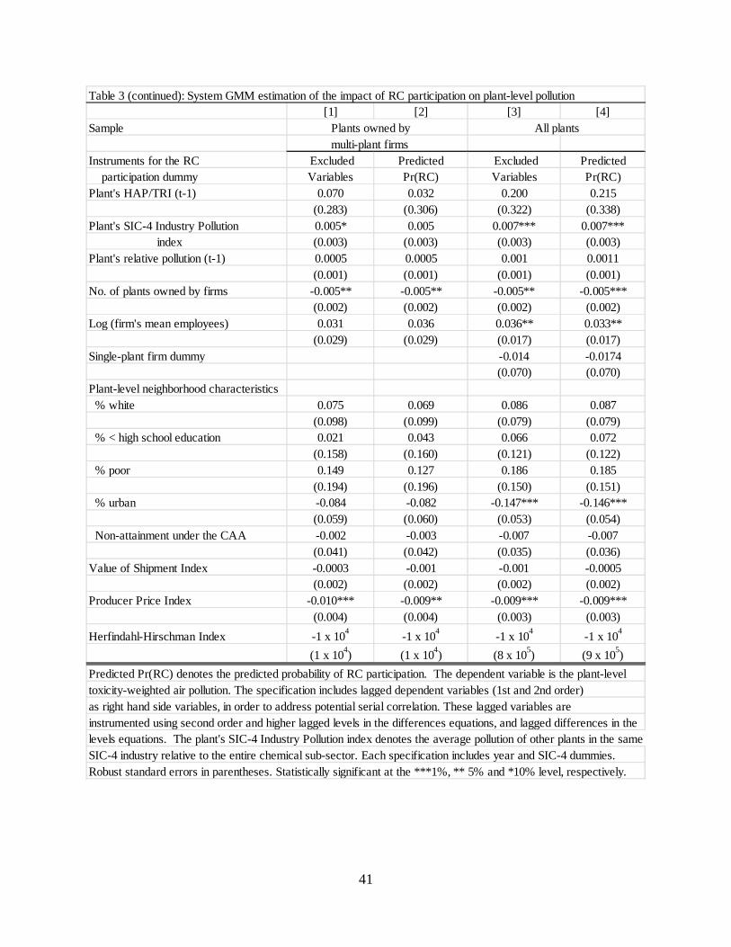
41

Table 3 (continued): System GMM estimation of the impact of RC participation on plant-level pollution [1] [2] [3] [4]

Sample Plants owned by All plants multi-plant firms

Instruments for the RC Excluded Predicted Excluded Predicted participation dummy Variables Pr(RC) Variables Pr(RC)Plant's HAP/TRI (t-1) 0.070 0.032 0.200 0.215

(0.283) (0.306) (0.322) (0.338)Plant's SIC-4 Industry Pollution 0.005* 0.005 0.007*** 0.007*** index (0.003) (0.003) (0.003) (0.003)Plant's relative pollution (t-1) 0.0005 0.0005 0.001 0.0011

(0.001) (0.001) (0.001) (0.001)No. of plants owned by firms -0.005** -0.005** -0.005** -0.005***

(0.002) (0.002) (0.002) (0.002)Log (firm's mean employees) 0.031 0.036 0.036** 0.033**

(0.029) (0.029) (0.017) (0.017)Single-plant firm dummy -0.014 -0.0174

(0.070) (0.070)Plant-level neighborhood characteristics % white 0.075 0.069 0.086 0.087

(0.098) (0.099) (0.079) (0.079) % < high school education 0.021 0.043 0.066 0.072

(0.158) (0.160) (0.121) (0.122) % poor 0.149 0.127 0.186 0.185

(0.194) (0.196) (0.150) (0.151) % urban -0.084 -0.082 -0.147*** -0.146***

(0.059) (0.060) (0.053) (0.054) Non-attainment under the CAA -0.002 -0.003 -0.007 -0.007

(0.041) (0.042) (0.035) (0.036)Value of Shipment Index -0.0003 -0.001 -0.001 -0.0005

(0.002) (0.002) (0.002) (0.002)Producer Price Index -0.010*** -0.009** -0.009*** -0.009***

(0.004) (0.004) (0.003) (0.003)Herfindahl-Hirschman Index -1 x 104 -1 x 104 -1 x 104 -1 x 104

(1 x 104) (1 x 104) (8 x 105) (9 x 105)Predicted Pr(RC) denotes the predicted probability of RC participation. The dependent variable is the plant-level toxicity-weighted air pollution. The specification includes lagged dependent variables (1st and 2nd order)as right hand side variables, in order to address potential serial correlation. These lagged variables are instrumented using second order and higher lagged levels in the differences equations, and lagged differences in thelevels equations. The plant's SIC-4 Industry Pollution index denotes the average pollution of other plants in the same SIC-4 industry relative to the entire chemical sub-sector. Each specification includes year and SIC-4 dummies.Robust standard errors in parentheses. Statistically significant at the ***1%, ** 5% and *10% level, respectively.

42

Table 4: Probit regression of RC participation on instrumental variables (IV) and other covariates.[1] [2] [3] [4]

Plants owned by All plants multi-plant firms No obs.=14,434 No obs.=22,822

Robust Robust Coeff. Std.Err. Coeff. Std.Err.†% RC participation in the SIC-4 (SIC-ProbRC) -14.06 *** 2.118 -12.58 *** 1.831†ACC membership in 1988 and 1989 (ACC) 2.329 *** 0.198 2.333 *** 0.176†Firm's HAP/TRI 0.588 ** 0.231†Firm's SIC-4 Industry Pollution index 0.005 0.004†Firm's plants' relative pollution -0.001 0.003†Firm's neighborhood characteristics % white 0.624 0.471 % < high school education -0.266 0.711 % poor 1.729 ** 0.812 % urban -0.584 * 0.299 County in non-attainment status under the CAA 0.208 0.210Single-plant firm dummy -0.111 0.247No. of plants owned by firm 0.050 *** 0.007 0.047 *** 0.008Log (firm's mean employees) 0.255 *** 0.078 0.160 *** 0.047Plant's pollution (t-1) 0.007 0.012 0.021 * 0.011Plant's HAP/TRI (t-1) 0.240 * 0.143 0.139 0.137Plant's SIC-4 Industry Pollution index -0.0001 0.003 0.001 0.003Plant's relative pollution (t-1) 0.0003 0.000 0.001 0.001Plant's neighborhood characteristics % white 0.089 0.176 0.008 0.162 % < high school education -0.121 0.263 -0.309 0.238 % poor 0.437 0.307 0.514 * 0.306 % urban -0.083 0.107 -0.128 0.094 Non-attainment county 0.120 0.078 0.078 0.077Value of Shipment Index -0.021 *** 0.005 -0.018 *** 0.004Producer Price Index -0.015 ** 0.007 -0.009 0.006Herfindahl-Hirschman Index -0.001 *** 0.000 -0.001 *** 0.000Constant 10.71 *** 1.869 10.09 *** 1.588Log-Likelihood -2,954 -3,834Likelihood Ratio Test - All Instruments 5,515 ***Likelihood Ratio Test - SIC-ProbRC, ACC 5,204 *** 6,340 ***Likelihood Ratio Test - Multi-Plant IVs 147 ***Notes: † denote variables that serve as the excluded variables in the main GMM specification. The plant's SIC-4 Industry Pollution index denotes the average pollution of other plants operating in the same SIC-4 industry relative to the entire chemical sub-sector. The firm's SIC Pollution index denotes the average SIC-4 Industry Pollution index of the subindustries in which the firm's plants operate. Each specification includes year and SIC-4 dummies. Statistically significant at the *** 1%, ** 5% and * 10%.

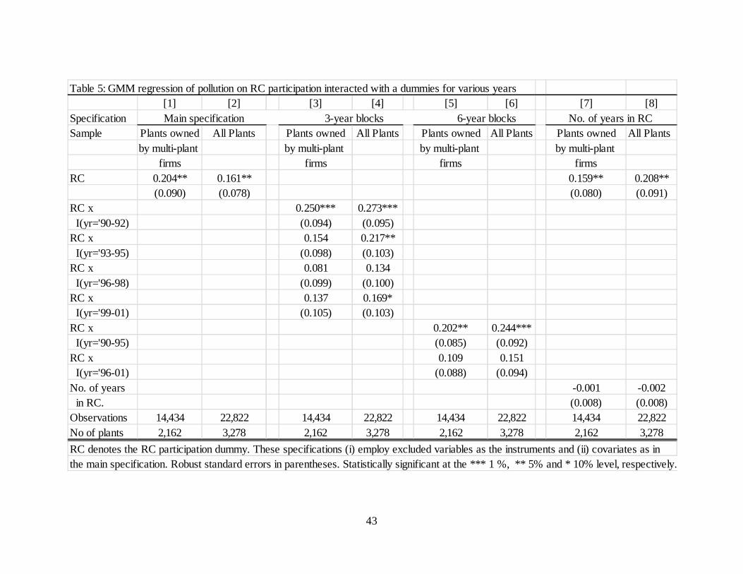
43

Table 5: GMM regression of pollution on RC participation interacted with a dummies for various years

[1] [2] [3] [4] [5] [6] [7] [8]Specification Main specification 3-year blocks 6-year blocks No. of years in RCSample Plants owned All Plants Plants owned All Plants Plants owned All Plants Plants owned All Plants

by multi-plant by multi-plant by multi-plant by multi-plant firms firms firms firms

RC 0.204** 0.161** 0.159** 0.208**(0.090) (0.078) (0.080) (0.091)

RC x 0.250*** 0.273*** I(yr='90-92) (0.094) (0.095)RC x 0.154 0.217** I(yr='93-95) (0.098) (0.103)RC x 0.081 0.134 I(yr='96-98) (0.099) (0.100)RC x 0.137 0.169* I(yr='99-01) (0.105) (0.103)RC x 0.202** 0.244*** I(yr='90-95) (0.085) (0.092)RC x 0.109 0.151 I(yr='96-01) (0.088) (0.094)No. of years -0.001 -0.002 in RC. (0.008) (0.008)Observations 14,434 22,822 14,434 22,822 14,434 22,822 14,434 22,822No of plants 2,162 3,278 2,162 3,278 2,162 3,278 2,162 3,278RC denotes the RC participation dummy. These specifications (i) employ excluded variables as the instruments and (ii) covariates as in the main specification. Robust standard errors in parentheses. Statistically significant at the *** 1 %, ** 5% and * 10% level, respectively.

44

Table 6: GMM regression of pollution on RC participation: heterogenous program effects

[1] [2] [3] [4] [5] [6] [7]Plants owned All Plants Plants owned All Plants Plants owned All Plants Plants ownedby multi-plant by multi-plant by multi-plant by multi-plant

firms firms firms firmsRC 0.204** 0.161** 0.186* 0.193** 0.137* 0.203** 0.159*

(0.090) (0.078) (0.112) (0.085) (0.082) (0.090) (0.082)RC x no. plants in firm 0.003 -0.001 that owns plant j (0.006) (0.005)RC x dummy for -0.23 single-plant firm (0.312)RC x firm's # -0.101 employees (t-1) (0.092)RC x % poor in plant's 0.370 0.458* neighborhood (0.234) (0.265)RC x % urban in plant's -0.003 -0.077 neighborhood (0.100) (0.129)Observations 14,434 22,822 14,434 22,822 14,434 22,822 14,434No. of plants 2,162 3,278 2,162 3,278 2,162 3,278 2,162Notes: RC denotes the RC participation dummy. The RC interaction variables are instrumented with the probit estimates of the probability of RC participationinteracted with the de-meaned covariates. Other covariates as in the main specification are included. Robust standard errors are in parentheses. Statistically significant at the *** 1%, ** 5%, and * 10% level, respectively.

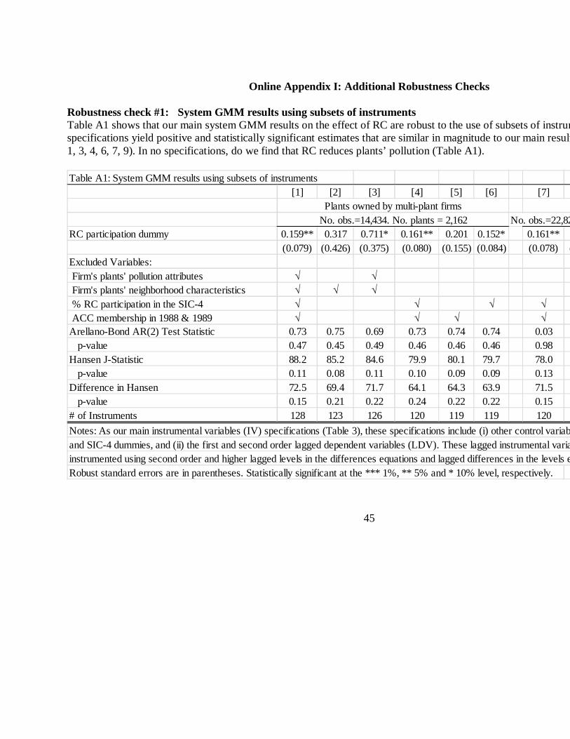
45

Online Appendix I: Additional Robustness Checks

Robustness check #1: System GMM results using subsets of instruments Table A1 shows that our main system GMM results on the effect of RC are robust to the use of subsets of instruments. Several specifications yield positive and statistically significant estimates that are similar in magnitude to our main results1, 3, 4, 6, 7, 9). In no specifications, do we find that RC reduces plants’ pollution (Table A1). Table A1: System GMM results using subsets of instruments

[1] [2] [3] [4] [5] [6] [7]

No. obs.=22,822. No. plants = 3,278RC participation dummy 0.159** 0.317 0.711* 0.161** 0.201 0.152* 0.161**

(0.079) (0.426) (0.375) (0.080) (0.155) (0.084) (0.078) (0.183)Excluded Variables: Firm's plants' pollution attributes √ √ Firm's plants' neighborhood characteristics √ √ √ % RC participation in the SIC-4 √ √ √ √ ACC membership in 1988 & 1989 √ √ √ √Arellano-Bond AR(2) Test Statistic 0.73 0.75 0.69 0.73 0.74 0.74 0.03 p-value 0.47 0.45 0.49 0.46 0.46 0.46 0.98Hansen J-Statistic 88.2 85.2 84.6 79.9 80.1 79.7 78.0 p-value 0.11 0.08 0.11 0.10 0.09 0.09 0.13Difference in Hansen 72.5 69.4 71.7 64.1 64.3 63.9 71.5 p-value 0.15 0.21 0.22 0.24 0.22 0.22 0.15# of Instruments 128 123 126 120 119 119 120Notes: As our main instrumental variables (IV) specifications (Table 3), these specifications include (i) other control variables, state, year and SIC-4 dummies, and (ii) the first and second order lagged dependent variables (LDV). These lagged instrumental variables areinstrumented using second order and higher lagged levels in the differences equations and lagged differences in the levels equations. Robust standard errors are in parentheses. Statistically significant at the *** 1%, ** 5% and * 10% level, respectively.

Plants owned by multi-plant firmsNo. obs.=14,434. No. plants = 2,162

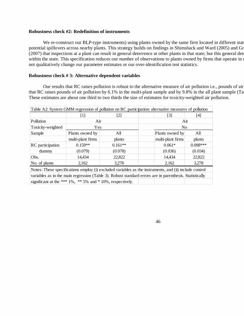
46

Robustness check #2: Redefinition of instruments

We re-construct our BLP-type instruments) using plants owned by the same firm located in different states to minimize potential spillovers across nearby plants. This strategy builds on findings in Shimshack and Ward (2005) and Gray and Shadbeg(2007) that inspections at a plant can result in general deterrence at other plants in that state; but this general deterrence is limited within the state. This specification reduces our number of observations to plants owned by firms that operate in multiple states, but did not qualitatively change our parameter estimates or our over-identification test statistics.

Robustness check # 3: Alternative dependent variables

Our results that RC raises pollution is robust to the alternative measure of air pollution i.e., pounds of air pollution. We find

that RC raises pounds of air pollution by 6.1% in the multi-plant sample and by 9.8% in the all plant sample (Table A2, column These estimates are about one third to two thirds the size of estimates for toxicity-weighted air pollution.

Table A2: System GMM regression of pollution on RC participation: alternative measures of pollution[1] [2] [3] [4]

Pollution Air AirToxicity-weighted Yes NoSample Plants owned by All Plants owned by All

multi-plant firms plants multi-plant firms plantsRC participation 0.159** 0.161** 0.061* 0.098*** dummy (0.079) (0.078) (0.036) (0.034)Obs. 14,434 22,822 14,434 22,822No. of plants 2,162 3,278 2,162 3,278Notes: These specifications employ (i) excluded variables as the instruments, and (ii) include control variables as in the main regression (Table 3). Robust standard errors are in parenthesis. Statisticallysignificant at the *** 1%, ** 5% and * 10%, respectively.

47

Online Appendix II: Propensity Score Matching (PSM) We use propensity score matching (PSM) as an alternative method to estimate the effect of RC. The PSM method, unlike the System GMM method, does not rely on the IV exclusion restrictions. The PSM estimates the average treatment effects on the treated. We apply several matching procedures as a check for robustness, i.e., kernel matching (Table A3, column 1), 5-nearest neigmatching (Table A3, column 2 and 3), 1-nearest neighbor matching (column 4 and 5). Our preferred estimates from the nearest neighbor matching procedure are matches with common support restrictions (Smith and Todd, 2005) The PSM estimates, particularly, those from kernel matching (0.147) and the 5-nearest neighbor matching with common support (0.169) are fairly similar in magnitude to our GMM estimates (0.159 to 0.204). The PSM estimate from the 1-nearest neighbor matching with common support (0.068) is about one third to almost one half the size of the GMM estimates. The PSM estimates, however, are not statistically significant at conventional levels.

Notes: Kernel matching uses all control observations in matching against the treated observations, but weights the observatiocloseness of the match using an Epanechnikov kernel. For the nearest neighbor procedures with the common support restrictionsexclude the treated observations whose estimated likelihood of treatment is greater than the highest estimated likelihood of untreated observations. When matching is done with replacement, a control case can be used more than once, allowing for more precise matching. We use a probit specification to generate our propensity score estimates.

Table A3: Propensity Score Matching (PSM) estimate of the impact of RC on plant-level pollution[1] [2] [3] [4] [5]

Matching procedure Kernel 5-Nearest Neighbors 1-Nearest NeighborWith replacement - Y Y Y YObservations All Common All Common All

Support SupportRC Participation, i.e., average 0.147 0.169 0.005 0.068 -0.139treatment on the treated (0.199) (0.167) (0.204) (0.198) (0.223)No. treated obs. (RC=1) 8,192 7,713 8,192 7,713 8,192No. control obs. (RC=0) 15,908 15,007 15,908 15,007 15,908

48

Online Appendix III: Impact of RC on plant-level pollution intensity

We examine the impact of RC on plant-level pollution intensity, defined as the ratio of toxicity-weighted air pollution to their number of employees. Lower pollution intensity would imply a more favorable trade-off between production and pollution (Cole et al., 2005); i.e., the same production would result in lower pollution.

We find that RC raises pollution intensity by 15.1% in the multi-plant sample (Table A4, column 3). We also find that

raises pollution intensity by 12.6% in the all plant sample (though we note that the instruments for the all plant sam(Table A4 column 4). We also use the alternative denominator of plant-level employee squared. We continue to find positive coefficients in both the multi-plant and all-plant samples, though these estimates are not statistically significant. We conclude that RC fails to reduce pollution intensity.

The alternative normalization strategy addresses one potential estimation issue from using the number of employee as the denominator. This estimation issue arises if plants respond to RC by choosing a production process that is less labor intensive, but that does not raise pollution per unit of production. Should larger plants increase their output at a faster rate than their use odenominator for large plants may be too small, resulting in too large a measure of pollution intensity. Given that RC participants

Table A4: System GMM regression of pollution on RC participation: alternative normalizations for pollution-intensity[1] [2] [3] [4] [5] [6]

Dependent variables are the ratio of toxicity weighted air pollution to different denominatorsDenominator (No. of employees)2

Sample Plants owned by All Plants owned by All Plants owned by All multi-plant firms plants multi-plant firms plants multi-plant firms plants

RC participation 0.159** 0.161** 0.151* 0.126* 0.111 0.052 dummy (0.079) (0.078) (0.078) (0.074) (0.074) (0.072)Obs. 14,434 22,822 14,293 22,640 14,293 22,640No. of plants 2,162 3,278 2,145 3,253 2,145 3,253Notes: These specifications employ (i) excluded variables as the instruments, and (ii) include control variables as in themain regression (Table 3). Robust standard errors are in parenthesis. Statistically significant at the *** 1%, ** 5% and * 10%, respectively.

No. of employees1

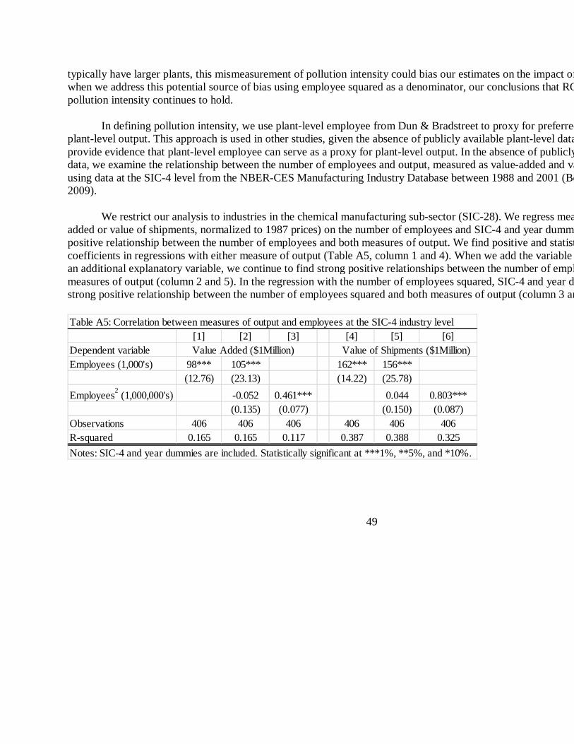
49

typically have larger plants, this mismeasurement of pollution intensity could bias our estimates on the impact of RC.when we address this potential source of bias using employee squared as a denominator, our conclusions that RC does not reducpollution intensity continues to hold.

In defining pollution intensity, we use plant-level employee from Dun & Bradstreet to proxy for preferred denominator of

plant-level output. This approach is used in other studies, given the absence of publicly available plant-level data (provide evidence that plant-level employee can serve as a proxy for plant-level output. In the absence of publicly available plantdata, we examine the relationship between the number of employees and output, measured as value-added and value of shipmentsusing data at the SIC-4 level from the NBER-CES Manufacturing Industry Database between 1988 and 2001 (Becker and Gray, 2009).

We restrict our analysis to industries in the chemical manufacturing sub-sector (SIC-28). We regress measures of output (value

added or value of shipments, normalized to 1987 prices) on the number of employees and SIC-4 and year dummies. Wpositive relationship between the number of employees and both measures of output. We find positive and statistically significant coefficients in regressions with either measure of output (Table A5, column 1 and 4). When we add the variable employee squared as an additional explanatory variable, we continue to find strong positive relationships between the number of employees and botmeasures of output (column 2 and 5). In the regression with the number of employees squared, SIC-4 and year dummies, we find strong positive relationship between the number of employees squared and both measures of output (column 3 and 6).

Table A5: Correlation between measures of output and employees at the SIC-4 industry level[1] [2] [3] [4] [5] [6]

Dependent variable Value Added ($1Million) Value of Shipments ($1Million)Employees (1,000's) 98*** 105*** 162*** 156***

(12.76) (23.13) (14.22) (25.78)Employees2 (1,000,000's) -0.052 0.461*** 0.044 0.803***

(0.135) (0.077) (0.150) (0.087)Observations 406 406 406 406 406 406R-squared 0.165 0.165 0.117 0.387 0.388 0.325Notes: SIC-4 and year dummies are included. Statistically significant at ***1%, **5%, and *10%.

50

Online Appendix IV: Factors associated with RC participation

Table A6: Factors that influence RC participation: marginal effects from the RC probit estimation[1] [2] [3] [4] [5] [6] [7] [8]

Plants owned by multi-plant firms (no. obs.=14,434) All plants (no obs.=22,822)dPr(RC) Std. Mean Std. ΔPr(RC) dPr(RC) Std. Mean Std. dX Error. Dev. due to 1 dX Error Dev.

Std. Dev.increase

% RC participation in the SIC-4 -5.408 0.862 0.291 0.165 -0.892 *** -3.668 0.518 0.269†ACC membership in 1988 and 1989 0.896 0.074 0.520 0.491 - *** 0.680 0.073 0.347Firm's HAP/TRI 0.226 0.090 0.847 0.278 0.063 **Firm's SIC-4 Industry Pollution index 0.002 0.002 4.642 9.552 0.019Firms' plants' relative pollution -0.0003 0.001 2.189 10.13 -0.003Firms' plants' average neighborhood % white 0.240 0.182 0.761 0.157 0.038 % < high school education -0.102 0.273 0.320 0.089 -0.009 % poor 0.665 0.317 0.158 0.082 0.055 ** % urban -0.225 0.115 0.720 0.239 -0.054 * Non-attainment under the CAA 0.080 0.080 0.619 0.283 0.023No. of plants owned by firms 0.019 0.003 13.32 12.34 0.236 *** 0.014 0.003 8.849†Single-plant firm dummy -0.032 0.070 0.329Log (firm's mean employees) 0.098 0.031 4.580 1.070 0.105 *** 0.047 0.013 2.896Notes: The marginal effects are calculated from the probit regression in Table 4. The probability of RC participation with values of covariates set at the sample mean is 0.21 for all plants and 0.60 for plants owned by multi-plant firms. The plant's SIC pollution index captures the plant's participation in higherpolluting sub-industries. Firms' plants' relative pollution is measured relative to other plants whose primary operations are in the same SIC-4 industry.† Impact on participation resulting from a discrete change from 0 to 1. Robust standard errors are reported. Statistically significant at the *** 1% level, ** 5% level and * 10% level, respectively.

51

Table A6 (continued): Factors that influence RC participation: marginal effects from the RC probit estimation[1] [2] [3] [4] [5] [6] [7] [8]

Plants owned by multi-plant firms (no. obs.=14,277)dPr(RC) Std. Mean Std. ΔPr(RC) dPr(RC) Std. Mean Std. dX Error. Dev. due to 1 dX Error Dev.

Std. Dev.increase

Plant's HAP/TRI (t-1) 0.092 0.056 0.747 0.394 0.036 * 0.041 0.039 0.752Plant's SIC-4 Industy Pollution index -0.00003 0.001 4.764 12.81 -0.0004 0.0002 0.001 4.128Plant's relative pollution 0.0001 0.0002 2.477 27.61 0.003 0.0002 0.0002 1.886Plants' neighborhood characteristics % white 0.034 0.068 0.762 0.283 0.010 0.002 0.047 0.759 % < high school education -0.047 0.101 0.328 0.165 -0.008 -0.090 0.071 0.327 % poor 0.168 0.118 0.160 0.151 0.025 0.150 0.090 0.158 % urban -0.032 0.041 0.714 0.406 -0.013 -0.037 0.027 0.736 †Non-attainment under the CAA 0.046 0.030 0.617 0.486 - 0.023 0.022 0.641Value of Shipment Index -0.008 0.002 94.9 12.94 -0.103 *** -0.005 0.001 94.82Producer Price Index -0.006 0.003 92.9 8.869 -0.052 ** -0.003 0.002 92.49Herfindahl-Hirschman Index -0.0004 0.0001 729 560 -0.204 *** -0.0002 0.0001 695Notes: The marginal effects are calculated from the probit regression in Table 4. The probability of RC participation with values of covariates set at the sample mean is 0.21 for all plants and 0.60 for plants owned by multi-plant firms. The plant's SIC pollution index captures the plant's participation in higherpolluting sub-industries. Plant's relative pollution is measured relative to other plants whose primary operations are in the same SIC-4 industry.Robust standard errors are reported. Statistically significant at the ***1% level, ** 5% level and * 10% level, respectively.

All plants (no obs.=22,822)

52

References for the Online Appendix Becker, Randy A. and Wayne B. Gray. 2009. “NBER-CES Manufacturing Industry Database:

Updated Data 1958-2005 - SIC and NAICS versions” Retrieved from http://www.nber.org/data/nbprod2005.html

Gray, Wayne B. and Ronald J. Shadbegian. 2007. “The Environmental Performance of Polluting Plants: A Spatial Analysis.” Journal of Regional Science 47(1): 63-84.

Holladay, J. Scott. 2010. “Abate or Abscond: Polluters’ Response to Environmental Regulation.” presented at the Georgia Institute of Technology economics seminar, October 2010.

Shimshack, Jay and Michael Ward. 2005. “Regulator Reputation, Enforcement, and Environmental Compliance.” Journal of Environmental Economics and Management 50(3): 519-540

Smith, Jeffrey A. and Petra E. Todd. 2005. Does Matching Overcome LaLonde’s Critique of Nonexperimental Estimators? Journal of Econometrics 125 (1-2) 305-353.