DOCTOR OF PHILOSOPHY - CORE

Multi-Agent Fitness Functions For Evolutionary Architecture

by

Richard Holden

A thesis submitted to the University of Plymouth in partial fulfilment for the degree of

DOCTOR OF PHILOSOPHY

School of Computing, Communications & Electronics Faculty of Technology

March 2005

Multi-Agent Fitness Functions for Evolutionary Architecture Richard Holden

Abstract

The dynamics of crowd movements are self-organising and often involve complex pattern formations. Although computational models have recently been developed, it is unclear how well their underlying methods capture local dynamics and longer-range aspects, such as evacuation. A major part of this thesis is devoted to an investigation of current methods, and where required, the development of alternatives. The main purpose is to utilise realistic models of pedestrian crowds in the design of fitness functions for an evolutionary approach to architectural design.

We critically review the state-of-the-art in pedestrian and evacuation dynamics. The concept of 'Multi-Agent System' embraces a number of approaches, which together encompass important local and longer-range aspects. Early investigations focus on methods-cellular automata and attractor fields-designed to capture these respective levels.

The assumption that pattern formations in crowds result from local processes is reflected in two dimensional cellular automata models, where mathematical rules operate in local neighbourhoods. We investigate an established cellular automata and show that lane-formation patterns are stable only in a low-valued density range. Above this range, such patterns suddenly randornise. By identifying and then constraining the source of this randomness, we are only able to achieve a small degree of improvement. Moreover, when we try to integrate the model with attractor fields, no useful behaviour is achieved, and much of the randomness persists. Investigations indicate that the unwanted randomness is associated with 2-lattice phase transitions, where local dynamics get invaded by giant-component clusters during the onset of lattice percolation. Through this in-depth investigation, the general limits to cellular automata are ascertained-these methods are not designed with lattice percolation properties in mind and resulting models depend, often critically, on arbitrarily chosen neighbourhoods.

We embark on the development of new and more flexible methodologies. Rather than treating local and global dynamics as separate entities, we combine them. Our methods are responsive to percolation, and are designed around the following principles: 1) Inclusive search provides an optimal path between a pedestrian origin and destination. 2) Dynamic boundaries protect search and are based on percolation probabilities, calculated from local density regimes. In this way, more robust dynamics are achieved. Simultaneously, longerrange behaviours are also specified. 3) Network-level dynamics further relax the constraints of lattice percolation and allow a wider range of pedestrian interactions.

Having defined our methods, we demonstrate their usefulness by applying them to laneformation and evacuation scenarios. Results reproduce the general patterns found in real crowds.

We then turn to evolution. This preliminary work is intended to motivate future research in the field of Evolutionary Architecture. We develop a genotype-phenotype mapping, which produces complex architecturcs, and demonstrate the use of a crowd-flow model in a phenotypefitness mapping. We discuss results from evolutionary simulations, which suggest that obstacles may have some beneficial effect on crowd evacuation. We conclude with a summary, discussion of methodological limitations, and suggestions for future research.

Contents

Acknowledgements X

Author's Declaration xi

1 Introduction 1 1.1 Overview of Research . 2

1.1.1 Thesis Outline . 2 1.1.2 Original Contributions 5 1.1.3 A Note on Style . 7

1.2 Evolutionary Algorithms . 7 1.3 Artificial Life ....... 10 1.4 Evolutionary Architecture 11 1.5 Architectural Components 12 1.6 Function and Form .... 13 1.7 Fitness Functions . . . . . 15 1.8 Models of Crowd Dynamics 16 1.9 Summary .......... 17

2 Pedestrian and Evacuation Dynamics I 18 2.1 Models ........... 18

2.1.1 Equation Models 19 2.1.2 Simulation Models 20

2.2 Multi-Agent Systems 21 2.2.1 Natural MAS .. 22 2.2.2 Virtual MAS .. 23 2.2.3 Pedestrian MAS . 24

2.3 Discrete Models . . . . . 26 2.3.1 Discrete Space . . 26 2.3.2 Coarse Network Representations . 26 2.3.3 Fine Network Representations 30 2.3.4 Space Syntax ... 33 2.3.5 Cellular Automata 34

2.4 Continuous Models 0 ••• 37 2.4.1 Continuous Space . 37 2.4.2 Fluid Dynamics . . 38 2.4.3 Steering Dynamics 39 2.4.4 Social Dynamics 39

2.5 Summary ••••••• 0 0 42

ii

3 Pedestrian and Evacuation Dynamics 11 44 3.1 Graph Theory .............. 44

3.1.1 Graphs ............... 44 3.1.2 Vector Walks on Simple Graphs . 47 3.1.3 Vector Walks on Constrained Graphs 47

3.2 Graph Theory: Applications 48 3.2.1 Space Syntax 48 3.2.2 Small Worlds 52

3.3 Attractor Fields . . 53 3.3.1 STREETS .. 54 3.3.2 EXODUS .. 57 3.3.3 Space Syntax 58 3.3.4 Summary .. 60

3.4 Local Dynamics . . . 60 3.4.1 Cellular Automata: Vehicle Traffic 61 3.4.2 Cellular Automata: Pedestrian Traffic 62

3.5 Summary .... • • • • • • • 0 ••••••• 0 63

4 Cellular Automata 67 4.1 1-D CA: Vehicles •••• 0 • 68

4.1.1 Statistical Behaviour 68 4.1.2 Summary .... 70

4.2 2-D CA: Pedestrians ... 70 4.2.1 Stable Behaviour 71 4.2.2 Testing Robustness 73 4.2.3 Statistical Behaviour 75 4.2.4 4-Directional Model . 77 4.2.5 Summary ...... 79

4.3 Extension of Pedestrian CA 80 4.3.1 New Rules for Pexchange . 81 4.3.2 Neighbourhoods and Graph Walks 83 4.3.3 Rule Extension for Moore Neighbourhoods 84 4.3.4 Summary •••••••• 0 ••••••••• 85

4.4 Coupling Cellular Automata with Attractor Fields . 86 4.4.1 Representing Obstacles . . . . . 87 4.4.2 CA-Based Model of Navigation 87 4.4.3 Summary 0 •• 0 • 89

4.5 Summary and Conclusion 90 4.5.1 Persistent Failure . 91 4.5.2 Reasons for Failure 92

5 Optimal Paths 93 5.1 Site Percolation on 2-lattice Graphs . 94

5.1.1 Percolation Threshold Pc 94 5.1.2 Pc: Implications . . . 96

5.2 Important Representations . 97 5.3 PCNN •••• 0 ••••••• 100

5.3.1 Artificial Neurons .. 100 5.3.2 Pulsed Neuron Model . 101

iii

5.3.3 Pulsed Neuron Dynamics . . . . . . 5.3.4 Pulse-Coupled Dynamics: 1-lattice 5.3.5 Pulse-Coupled Dynamics: 2-lattice 5.3.6 Summary . . . . . . . . . . . .

5.4 PCNN: Relevance to Egress Modelling 5.5 Robust Autowaves . . . . . . . . . . .

5.5.1 Pitfalls in PCNN Equations .. 5.5.2 Enhanced Autowave Equations 5.5.3 Complex Search .

5.6 Summary . . . . . . . . . . . . . . . .

6 Egress Modelling 6.1 Efficient Autowaves . . . . . . .

6.1.1 2-D Cellular Automata . 6.1.2 CA-Ba.sed Autowaves .. 6.1.3 Example Search in Arbitrarily Complex Configurations 6.1.4 Tra.ceba.ck Algorithm 6.1.5 Summary . . . . . . . . . . . . .

6.2 Multi-Agent Scenarios . . . . . . . . .. 6.2.1 Movement and Multiple Optima . 6.2.2 Multi-Agent Representation . 6.2.3 Inclusive Search: Limits . . . 6.2.4 Use of Time Series Signatures 6.2.5 Dynamic Search Boundaries . 6.2.6 Summary . . . . . . . ....

6.3 Simulation Models: Pedestrian Pattern Formation 6.3.1 Lane-Formation . 6.3.2 Egress . . 6.3.3 Summary

6.4 Summary ....

7 Evolutionary Architecture 7.1 Nature-Inspired Growth

7 .1.1 Social Insects . . 7 .1. 2 Crystal Aggregation 7.1.3 Summary .... .

7.2 Architectural Spaces ... . 7.3 Developmental Algorithm .

7.3.1 Diffusion and Construction . 7.3.2 Diffusion and Construction: Constraints 7.3.3 Summary ........ .

7.4 Artificial Evolution . . . . . . . . 7.4.1 Simple Genetic Algorithm 7.4.2 Evolutionary Dynamics ..

7.5 Evolution: Generative Architecture 7.5.1 Genotype r-> Phenotype 7.5.2 Genetic Algorithm ... . 7.5.3 Phenotype r-> Fitness .. . 7.5.4 Evolutionary Simulation 1

iv

103 104 105 108 109 110 111 112 115 118

119 119 120 121 124 126 126 128 128 129 130 133 136 140 142 142 145 146 148

149 150 150 152 156 156 157 158 161 164 166 166 168 169 170 174 175 175

7.5.5 Summary .............. 179 7.6 Evolution: Constrained Architecture ... 180

7.6.1 Genotype t-+ Phenotype t-+ Fitness 180 7.6.2 Evolutionary Simulation 2 182

7.7 Summary •••••••••• 0 ••• 0 • 0 0 182

8 Conclusion 185 8.1 Thesis Summary •••••••••• 0 • 185

8.1.1 Background: Crowd Dynamics . 185 8.1.2 Limits to Locality: Percolation 186 8.1.3 Solution: Inclusive Search, Simple Dynamics 187 8.1.4 Evolutionary Approach . 189

8.2 Future Directions . . . . . . . . 190 8.2.1 Concepts of Space . . . . 190 8.2.2 Developmental Codings . 192

8.3 Closing Comments •••• 0 0 • 193

A Glossary 195

B CA Rule Set Extensions 199

c Publications 201

Bibliography 231

V

List of Figures

2.1 A simple example of emergent behaviour 2.2 Different types of networks ........ . 2.3 Enclosed configurations as coarse networks 2.4 Enclosed configurations as fine-grained networks 2.5 Isovist and isovist field 2.6 CA scheme . . . . . . . . . . . . . . . . . . . 2.7 CA dynamics ................. . 2.8 Cellular Automata model of simple movement 2.9 Simple, continuous movement 2.10 Helbing's social force model ...

3.1 Elements and structure of graphs 3.2 Vector walk on a 2-lattice .... 3.3 Constrained graphs and movement 3.4 Spatial configurations and locality . 3.5 Depth values for a one-dimensional space 3.6 Configuration depth against space size 3. 7 Components of coJnmw1ities . . . . . 3.8 A shopping mall model in STREETS 3.9 Depth information in EXODUS .. 3.10 Fragmentation of a spatial graph 3.11 Nagel and Rasmussen's vehicle CA 3.12 Blue and Adler's pedestrian CA ..

4.1 Nagel and Rasmussen's model at varying density . 4.2 Statistical properties of the Nagel and Rasmussen (1996) CA 4.3 Directional and 2-directional speed-density statistics . 4.4 More snapshots of the Blue and Adler model . 4.5 Frozen patterns in the pedestrian CA . . . . 4.6 Travel-time properties of the pedestrian CA 4.7 2-directional and 4-directional behaviour ... 4.8 Conflicts in 2-directional and 4-directional populations 4.9 Results of local, density-determined exchanges . . .. 4.10 Optimal walks for three different spaces ....... . 4.11 Relationships between discrete and continuous spaces 4.12 Relationship between 4 and 8-directional behaviour 4.13 Representing complex configurations ...... . 4.14 Complex, non-periodic configurations ...... . 4.15 Travel time comparison for various configurations 4.16 Graphical snapshots of the pedestrian model

vi

23 27 28 31 33 35 35 36 40 41

46 48 49 50 50 51 53 55 58 59 61 65

69 70 72 74 75 77 78 79 83 84 85 86 87 88 89 91

4.17 Components of search in CA models

5.1 Percolation on a Boolean network .. 5.2 Critical percolation transitions .... 5.3 Effect of critical point of interaction . 5.4 Real and artificial neurons . . . . . . 5.5 Dynamics of a pulse-coupled neuron . 5.6 Autowaves in non-periodic, 1-lattice media 5.7 Time series signatures ...... . 5.8 Autowave behaviour . . . . . . . . . . . 5.9 PCNN as a shortest path algorithm . . . 5.10 Walks determined by threshold functions 5.11 PCNN scheme for pure autowaves ... 5.12 Example autowaves on 2-lattice PCNN 5.13 Simple and complex configurations 5.14 Autowave configuration signatures.

6.1 Langton's ant ........... . 6.2 Pulse-coupled logic for single vertex 6.3 Network logic . . . . . . 6.4 Configuration signatures . 6.5 Traceback subgraph . . . . 6.6 Sampled graph trajectory 6.7 Adaptive graph trajectory 6.8 Wave exploration in occupied space 6.9 Redundancy in wave exploration . . 6.10 Simple and complex trace-back graphs 6.11 Fraction of one-type signatures . . .. 6.12 Conditional probability of failure in one-type signatures . 6.13 Search boundaries using time-series information 6.14 Distribution of post type-one search . 6.15 Radius against density . . . . . . . . . . 6.16 Relaxation method . . . . . . . . . . . . 6.17 Comparison of lane formation behaviour 6.18 Two-door, two-exit configuration . . 6.19 2-directional flows in a configuration ..

7.1 Architectural form in a model of nest assembly. 7.2 Branching architectures of Witten and Sander's DLA. 7.3 Various branching architectures of D'Souza and Margolus' DLA. 7.4 Representations of architectural space ....... . 7.5 Evolved architectural forms ............... . 7.6 Configuration development (Pan! = 0.001, Pseed = 0) ... . 7.7 Configuration development (Pan! = 0.001, Pseed = 0.0001) 7.8 Configuration development (Pant= 0.01,Pseed = 0.0001) .. 7.9 Fragmented space. . . . . . . . . . . . . . 7.10 Variety of single component configurations. 7.11 Fitness landscape .......... . 7.12 Genetic encoding of ants and seeds .... .

vii

92

95 96 98

100 103 104 107 108 109 112 113 115 116 117

122 123 124 125 127 129 130 132 133 135 136 137 139 140 141 143 145 146 147

151 152 154 157 157 160 161 162 163 163 168 171

7.13 Genetic encoding of exits. . .. 7.14 Genotype arrangement ..... 7.15 Oscillatory patterns in ant CA . 7.16 Example phenotypes .... . 7.17 GA Evolution ........ . 7.18 GA Evolution (configuration) 7.19 GA Evolution (depths) 7.20 Portland Square ... 7.21 Random phenotypes 7.22 Exit-sign evolution . 7.23 Exit-sign phenotypes

8.1 Spatial arrangements of hydrogen and oxygen 8.2 The honeycomb lattice

B.1 Neighbourhoods ....

viii

171 172 173 174 177 178 179 181 181 183 183

190 192

199

List of Tables

2.1 Shortest Path Algorithm . . . . . . . 29

3.1 Pedestrian Cellular Automata Rules. 64

5.1 PCNN Algorithm for Clean, Expanding Autowaves 114

6.1 Langtons' 'Ant' Cellular Automata 121

7.1 Modified Version of Langton 's Ant 159 7.2 Construct Mode . . . . . . . . . . . 159 7.3 High-Level Description of Developmental Algorithm 165 7.4 Simple Genetic Algorithm ...... 167 7.5 Our Genetic Algorithm . . . . . . . . 176

B.1 Pedestrian Cellular Automata Rules . 200

IX

Acknowledgements

I gratefully acknowledge Ian Parmee for supervising me in the early stages of this work and for giving me this opportunity. Thanks also to Ken Fisher for the criticisms of early ideas.

I am equally as grateful to Angelo Cangelosi for taking over the role of first supervisor on Ians departure, not only with such enthusiasm, but with my best interests at heart and for his encouraging support-thanks Angelo.

I have good memories of sharing an office with Dominic Mitchell, Stalin Munoz and lan Packham-thanks for all your help and for being such good company.

I took some well-spent time away from the PhD. I am grateful to Robert Shipman (cheers Rob) and the rest at the Intelligent Systems Lab, Btexact. I would like to thank Ann SeiferleValencia and Neville Sanjana for their company on the CSSS mini-project, Tom Carter for the enthusiastic advice on it, and especially Paul Brault from the Santa Fe Institute for organising everything. Angelo, thanks for letting me go (and asking me to come back).

In the last ten months, while writing up, I have had the good fortune to have been found a very quiet and cosy office in Portland Square and for this I am grateful to Phi! Dyke. I have been able to really concentrate here-many thanks.

More generally, various strands in the School of Computing have provided a vibrant research community during my time here. In particular, the Engineering Design Centre, the Centre For Neuml and Adaptive Systems and the Centre for Intemctive and Intelligent Systems. I would like also to single out Roman Borisyuk, whose limitless enthusiasm for arranging internal and external seminars over the years has been a vital source of stimulation. I would also like to thank Jason Kinser from Georye Mason University for useful e-mail comments on the PCNN stuff, lan Burkitt from the University of Bmdford for encouraging me into postgraduate study in the first place, and Aclrian Stanley for sending me a copy of his MSc thesis (Stanlcy, Hl92), which was very useful in the early stages.

Most importantly of all, I want to thank my family-Mum, Danielle & Simon, Joseph, Tom, Dad & June-for your love & support and for all being there on my visits 'up-north', and yours 'down-south'. I often think of and miss you all. In particular, special thanks to you Mum. Your love and encouragement to do what makes me happy means the world to me-thanks for everything. Special thanks to my girlfriend Pauline; I am lucky and grateful for your patience and loving care. Thanks for the proofreadiug(s) and sorry for asking you so often xx.

X

Author's Declaration

Declaration:

At no time during the registration for the degree of doctor of Philosophy has the author been registered for any other University award.

This study was financed with the aid of a University of Plymouth studentship.

A programme of advanced study was undertaken and relevant scientific seminars and conferences were regularly attended. Work was presented and published.

Publications:

A preliminary vision of the project was presented as a poster (Holden and Parmee, 2000) based on preliminary work, none of which is contained herein. Since that preliminary work, and with further investigations, the project changed emphasis. These investigations have been reviewed, presented and published (Holden and Cangelosi, 2004b), based on the work, which underpins chapter 5. Another publication, which contains details of our general methodology was reviewed, presented and published (Holden and Cangelosi, 2004a), based on the work which underpins chapter 6. These three publications are contained within the appendices (see Appendix C).

A further publication resulted from work at a summer school (Holden, Sanjana and SeiferleValencia, 2002). This is not directly relevant to the thesis, but informed an analysis of those models outlined herein, which attempt to exploit statistical techniques based on Small World theory.

Conferences Attended:

ACDM 2000, University of Plymouth, Plymouth. Complex Systems Summer School 2002, Santa Fe Institute, Santa Fe. Inteflam 2004, Heriot-Watt University, Edinburgh.

Industrial Work:

Between 10/2001 and 08/2002, work was undertaken in the Intelligent Systems Lab, BTexact. This inspired some of the ideas developed in Chapter 5 on pulsed neural networks.

Word Count = 45, 925, inc. captions and appendices.

Signed ......... .!k/1~/~ ................... . Date ............. !b/.~ .. ~>.: .................. ..

xi

IQ' loving :memory :of 1Elsie HorQt:J.

xii

Chapter 1

Introduction

Egress refers to the process of movement in populations of pedestrians. Each pedestrian must

move within a built configuration, from a given origin location to a destination location. There

are a number of complexities involved, which incorporate configuration-pedestrian interactions

and pedestrian-pedestrian interactions. Also, both kinds of interaction can take place at

varying degrees of locality. One problem is to represent such complexities at an appropriate

level of abstraction, so that we can build models that capture real pedestrian flows.

Our longer-term aim is to utilise egress models as fitness functions in an evolutionary ap

proach to the design of building architecture. However, an essential first step is, of course, to

develop sound models. Most of the thesis is devoted to the latter, but after successfully mod

elling important aspects of real crowds, we also manage to provide a preliminary evolutionary

approach to the former. The main purpose of this chapter is to set the background of the

thesis, both in terms of our longer-term aims, and the immediate problem of egress modelling.

We provide an overview, which outlines the thesis structure and contributions (Section

1.1). We introduce a number of relevant fields of enquiry and concepts; Evolutionary Al

gorithms (Section 1.2), Artificial Life (Section 1.3), Evolutionary Architecture (Section 1.4),

methods of architectural decomposition (Section 1.5), and the concepts of function and form

in an evolutionary sense (Section 1.6). We introduce the meaning of fitness functions in an

1

evolutionary-algorithmic sense (Section 1.7) and the field of Crowd Dynamics (Section 1.8).

While doing this we hook-on particular beliefs and general aims, which we summarise at the

end of the chapter (Section 1.9).

1.1 Overview of Research

1.1.1 Thesis Outline

Chapter 2: We address the broad aspects of scientific modelling in order to identify an ap-

propriate level of abstraction for models of egress behaviour. We introduce the idea of

a Multi-Agent System (MAS) and refer to pedestrian crowds as examples of such sys-

terns. We critically review some egress and crowd dynamics models from the literature,

introduce the concepts on which these models are based and identify issues relevant

in an evolutionary context 1. We organise this review around concepts of discrete and

continuous space, and indicate which techniques from both are worth looking at in more

detail.

Chapter 3: Having abandoned a number of modelling approaches, we offer a more detailed

technical review of the methods, which underpin models that remain relevant to our

chosen level of abstraction. The aim is to introduce the details of computational rep-

resentations used and, therefore, identify in more detail which kinds of pedestrian be-

haviours are important and at what level model dynamics should be specified. In this

way, chapter 3 is a more detailed expose of the methods previously ring-fenced as poten-

tially useful in Chapter 2. As a result of this more in-depth review, further modelling

techniques are deemed inappropriate in accordance with our aims. We are left with the

approaches, which utilise Cellular Automata (CA) methods or field attractors, which

'Throughout the thesis we use the terms egress and crowd dynamics interchangeably because their meaning is often interwoven. However, it is also useful to think of egress as the general processes and patterns of crowd behaviours that occur when a crowd population vacates a conHguration. Crowd dynamics refer to the rules that give rise to these patterns as the process of egress unfolds. The reader may also find the glossary in Appendix A useful for definition of other terms.

2

capture local and global dynamics, respectively.

Chapter 4: We replicate and thoroughly investigate the properties of aJl existing CA model.

We choose a well-published model from the literature and attempt to analyse its be

haviour. The model is designed to produce important dynamic patterns found in popu

lations of real crowds. Based on our evidence, we argue that this CA is inadequate. The

problem stems from an underlying attempt to model complex and high-level behaviours

from the development of overly simple rules, which operate in limiting local neighbour

hoods. We therefore attempt to incorporate the local dynamics of the CA with a global

attractor field. The aim is to integrate local with global methods, in order to model the

short and long-range behaviours, observed in real pedestrian crowds. However, we fail

to meet our aims and this approach is taken no further.

Chapter 5: One property of the CA, observed from the investigation of Chapter 4, is the

sudden collapse of intended pattern formation and a phase transition between a relatively

stable behavioral regime and a behavioral regime associated with large-scale randomness.

Following on from these observations, we take a detailed look at the nature of information

interaction in 2-lattice graphs. The 2-lattice is assumed in almost all discrete, MAS

models of pedestrian and evacuation dynamics. If we are to model interactive systems

by using this kind of lattice, then we need to understand the properties of this spatial

domain. We replicate results from the field of computational physics and investigate

information percolation on the 2-lattice. We present statistical results, which show phase

transition behaviours of the 2-lattice space. We also show how these phase tr8JlSitions

define an upper limit to the success of any rules specified in local neighbourhoods.

This chapter is, therefore, the point where we abandon any attempt to specify rules at

a purely local level, ru1d the hope of any higher-level emergence of global dynamics from

such localities. We suggest reasons why localised models of egress behaviour might be

generally limited, and what is required to represent local interactions between agents

3

and more global strategies of escape. These requirements lead us to the introduction of

the Pulse Coupled Neural Network (PCNN). Most of this chapter is then dedicated to

the investigation of a pulsing neuron model and coupled populations. Originally applied

in the area of image processing, PCNN's have been shown to produce clear and well

defined patterns of autowave expansion. We argue that in view of 2-lattice properties

these expanding waves may offer an alternative and more robust method of search in

local neighbourhoods. We enhance autowave features by pruning neuron equations. We

demonstrating how this model may be useful in the specification of appropriate dynamics

for pedestrian egress behaviours.

Chapter 6: Results from Chapter 5 provide a basis for a new approach to modelling pedes

trian dynamics and egress. Instead of using the disparate methods of other approaches,

such as locally defined CA and globally defined attractor fields, this new approach

integrates the local and global perspective. We provide a complete description of a

multi-agent system, capable of modelling adaptive behaviour in a population of escap

ing individuals. This system is based on a dynamic boundary, which defines locality, and

is derived from time series information in autowave expansions. Essentially, this method

provides a robust region around a pedestrian, which is able to return useful information

without suffering the catastrophic effects of lattice space.

We demonstrate the potential use of these tools in modelling pedestrian evacuation

scenarios with two models, which reproduce crowd behaviour patterns found in real

crowds.

Chapter 7: By producing models of the real emergent patterns found in actual crowds, we

are confident enough to then take a step back from the detail of modelling and look

forward to our longer-term aims. We provide a preliminary demonstration of how the

model might be used in future evolutionary approaches to the design of architectural

space. This chapter is preliminary in the sense that we use a restricted density param-

4

eter, due to 2-lattice constraints. We present two evolutionary simulations. The first

depends on a nature-inspired algorithm, which automatically develops valid architec

tural representations of space. The second is a constrained application of evolution to

the optimisation of exit-sign locations. We introduce an evolutionary algorithm, and a

genotype ~----> phenotype ~----> fitness mapping for both evolutionary simulations. Although

we should treat these preliminary results with caution, they demonstrate both useful

selection pressure and the efficacy of evolution in the functional optimisation of building

design.

Chapter 8: We critically summarise the thesis in the light of original aims. Conclusions are

drawn and possible future directions considered.

1.1.2 Original Contributions

Five central contributions are made:

1. Investigation into Cellular Automata model (see Chapter 4):

(a) We replicate a number of CA models and design statistical teclmiques, which pro

vide indicators of model breakdown.

(b) We attempt to improve the rule sets by introducing methods, which reduce inherent

randomness. This improves some of the runaway random effects in the CA.

(c) However, further investigation reveals that intended pattern formations fail catas

trophically as density parameters increase.

2. Fundamental limitations of local methods (see Chapters 4 and 5):

(a) By considering the interaction complexities typical in percolation studies of the 2-

lattice graph we offer reasons as to why 2-D CA models fail catastrophically. This

has important implications as to:

i. how to represent dynamics and

5

ii. how to specify egress models.

3. Investigation into pulsed neuron properties in a Multi-Agent System approach to crowd

modelling (see Chapter 5):

(a) We develop ideas derived from studies of the Pulse Coupled Neural Network (PCNN).

(b) We argue that the PCNN provides a more adequate, network-level search and

demonstrate how when tuned appropriately, spaces of high complexity are explored.

(c) We identify a number of useful properties in these networks and adapt equations

in order to enhance these properties.

4. Efficient implementation of autowave search (see Chapter 6):

(a) We implement a simplified version of the search algorithm because the PCNN is

computationally expensive, particularly in multi-agent scenarios.

(b) We execute network search through the implementation of a locally executable CA,

which has two primary advantages:

1. arbitrarily complex networks can be explored.

ii. computational cost is reduced.

5. Techniques for the development of models for egress scenarios (see Chapter 6}:

(a) We present general methods for model specification.

(b) In order to demonstrate the potential power of our tools we produce two models,

which replicate important optimising behaviour found in real crowds. The first

model achieves this in simple spatial configurations and the second in more complex

spatial domains. These models serve to demonstrate the self-organising potential

of our approach and provide a rationale for utilising such techniques as fitness

functions for evolutionary architecture.

6

6. Multi-agent fitness functions for evolutiona1'1J architecture (see Chapter 7):

(a) We preset details of a developmental algorithm, which can be used to generate an

arbitrary amount of spatial configurations with various levels of complexity.

(b) We present details of Genotype>-+Phenotypes>-+Fitness mappings and present evo

lutionary results, using the fitness function in the context of two different kinds of

evolutionary simulations.

1.1.3 A Note on Style

There is no pre-ordained style to every chapter, although we have decided to adhere to some

organising principles while writing. Each chapter firstly contains an abstract-styled overview

of its contents. This is intended to provide a general feel for the chapter before details appear.

At the end of each chapter a summary recaps the main concepts, results and/or arguments

and provides a bridge to the following chapter. Where we feel a section inside a chapter has

been particularly long or detailed, we provide a similarly styled summary, but local to that

section.

We now begin our introduction to the general fields of enquiry and concepts, which motivate

and are implicated in the work of this thesis.

1.2 Evolutionary ·Algorithms

Since Darwin, it has been possible to think of the latest end products of evolution as man

ifestations of a plodding accumulation of small, adaptive change. Complex phenotypes are

selected over millennia and their foriiiS are shaped by relentless environmental pressures. Con

sidering how complex some of these forms are, it has been difficult to imagine how these form

have arisen, other than through the skill of a conscious creator. But in spite of our imagina

tion, or perhaps because of a different, scientific one, evidence suggests that Darwins theory is

correct-given the right building materials, nature juggles them, with stunning creativity, into

7

the beautiful configurations that we call 'life'. Yet, despite its appearance and true to form,

nature appears to follow a comparatively simple set of rules, which convert matter into life.

Although fine-grained details of natural evolution are not fully understood, at another level,

general Darwinian process can be viewed as algorithmic; as a program of change executed in

the medium of nature (Dennet, 1995). On this view, it is not a necessary condition that selec

tion be implemented only in accordance with natural constraints. The implication is that that

fundamental Darwinian mechanisms (Variation, Inheritance, Reproduction, Mutation) can be

implemented in other media. In the past thirty years strides have been made in computer

based evolution and today Evolutionary Algorithms are a huge and various industry, the GA

(Holland, 1975; Goldberg, 1989) being the most popular and widely used (Bently, 1999).

The general aim of all Evolutionary Computation is to exploit scientific ideas about natu

ral, solution-driven innovations in the face of a ceaseless, selection-driven process of survival.

Questions are open regarding the detailed accuracy of Evolutionary Algorithms as appropri

ate representations of real biological populations. For example, the fundamental Darwinian

processes found in natural evolution are not always well represented, but the GA is perhaps

the most extensive evolutionary algorithm in this respect (Bently, 1999). This said, we are

not directly interested in biological details other than for their adaptive properties. In this

sense we do not intend to construct a model of evolution, but rather exploit its power in the

context of design. We will encounter some of the specific GA mechanisms later in the thesis,

but for now two general concepts suffice; 'exploration' and 'exploitation':

Exploration involves the discovery of new solutions. As in biology, GA's operate on geno

types where probabilistic mutations occur at given sites. Mutations introduce the pos

sibility of innovations, which might contribute to the overall fitness of a phenotype.

Without mutation, GA's can only accumulate random pieces of information and evo

lution is likely to stagnate with early convergence to poor solutions. The concepts of

innovation and stagnation are combined in a population-dependant concept of fitness,

where each population member is judged according the the fitness of the entire popu-

8

lation. Innovations through mutation, over time, come to dominate the population and

this is where the second concept, exploitation, derives its meaning.

Exploitation produces an accumulation of information, which contributes positively to fit

ness. In biology, the dominant view is that genes are the selected units (Dawkins, 1976)

and, although provisional, fit genetic material tends to accumulate in phenotypes. Any

fit genes are, by implication, more likely to survive because they contribute to the sur

vival of the phenotype carrier. Because phenotypes reproduce with inheritance, and

hence accumulate genetic information, even though mutations explore genotypes, a

species' genetic historical identity is stubbornly apparent due to this selective pressure.

For example, phenotypes as different as humans and rats share large amounts of genetic

material, which in a Darwinian interpretation, is inherited from an origin-points in

biological history where a species began to branch into separate reproductive futures.

Although evolution clearly innovates through mutation, and diverges from this origin

over time, there is always this power to exploit.

By analogy to these biological process, Holland argues that artificial evolution selects build

ing blocks. Just like we combine known strategies in solving a new problem, building blocks on

binary strings are combined through a process akin to sexual reproduction (Holland, 1975; Hol

land, 1995). These building blocks contribute to the success of the entire string and 'good'

building blocks accumulate and persist, both over time and across a population, even though

mutations keep on exploring. In short, the GA is a multi-tasking algorithm. It harnesses both

explorative and exploitative forces. Any conference proceeding on GA's over the last ten years

will testify to the great amount of research dedicated to these general properties of the GA.

These mechanisms need to be tuned to the particular application domain and thus various

techniques based on explorative and exploitative forces have arisen in Evolutionary Design

(For example, Parmee, 2000).

9

1.3 Artificial Life

Whereas EA's have a clear and singular, nature-inspired foundation, A-Life is more generally

nature-inspired. According to Bonabeau and Theraulaz, it is a "method consisting in gen

erating at a macroscopic level, from microscopic, generally simple, interacting components,

behaviours that are interpretable as lifelike" (p 303, Bonabeau and Theraulaz, 1995). This

definition broadly captures many activities in A-Life approaches, but A-Life has many faces

and other fields of enquiry often cut across it. For example, in the study of adaptive agents,

techniques such as Artificial Neural Networks and GA's are used. Many scientists in the field

of A-Life often find that they have to define what is artificially life-like in their work. But there

are concepts that define the field, even if they are shared with other domains (Boden, 1996a).

In the definition provided by Bonabeau and Theraulaz, generating is a very useful term for

our current purposes. A generative procedure is one where simple rules interact and develop

into higher-level patterns. A good example are CA, collections of low-level, locally interactive

rules, which develop into global patterns. Generative procedures are part of many 'bottom-up'

approaches, but are particularly important in A-Life-interactions between artificial units may

produce significantly interesting patterns in comparison with those found in natural systems

(Langton, 1996a). Maybe the biological medium is also not a necessary condition for the

production of life-like behaviour, just as Dennet (1995) argues in terms of evolution? Some

even claim that certain computerised behaviour is life rather than life-like, leading to the

internal separation of the so-called 'strong' and 'weak' A-Life brigades (Levy, 1993).

Good examples of generating procedures are fow1d in the new field of computational mor

phogenesis, where preliminary work investigates complex mappings between the genotype and

the phenotype (Kurnar and Bentley, 2003; Stanley and Miikkulainen, 2003). Tools in this field

include CA, L-Systems and various other self-organising techniques. A general theme in com

putational morphogenesis is to analyse the nature and complexity of the mechanisms that

control the process of development. Prusinkiewicz (1995) suggests that morphogenesis can be

used in fields as far from theoretical biology as graphic design, computer art and landscape

10

architecture. Developmental procedures are therefore useful in domains other than theoretical

biology. This is true of the field of Evolutionary Architecture, which we now introduce.

1.4 Evolutionary Architecture

We have so far presented Artificial Evolution and A-Life separately, but nowhere are over-

laps more apparent than in this new domain. Evolutionary Architecture was conceived by

Frazer (1995) and refers to architecture in the sense of man-made building design. Evolution-

ary Architecture is interdisciplinary and various techniques from the field of computational

intelligence are used. As Frazer states:

"An evolutionary architecture investigates the fundamental form-generating processes in architecture, paralleling a wider scientific search for a theory of morphogenesis in the natural world. It proposes the model of nature as the generating force in architectural form. The profligate prototyping and awesome creative power of natural evolution are emulated by creating virtual architectural models, which respond to changing environments... Architecture is considered as a form of artificial life, subject, like the natural world, to principles of morphogenesis, genetic coding, replication and selection. "

(p 9, Frazer, 1995)

Frazer's work on evolutionary architecture is mostly speculative, but he does outline some

of the computational techniques, which may be useful for the future of the field. He includes

Artificial Neural Networks (ANN's), Classifier Systems, the CA and CA among his list. Since

Frazer's (1995) book, a small but growing group of computer scientists are beginning to apply

techniques mentioned by Frazer for evolving architectural forms. Architecture per se is pri-

marily concerned with space, structure and form and Evolutionary Architecture is concerned

with decomposing these concepts into primitive units, expressing these in generative rules,

which can be genetically coded, developed, tested and evolved (O'Reilly and Testa, 2000).

Also, CA have been used to try and explore the fundamental rules of form in architecture

(Broughton, Tan and Coates, 1997; O'Reilly and Testa, 2000). This work defines a small, but

growing trend in the use of nature-inspired computation for evolutionary architectural design.

11

Unlike the majority of GA applications, Evolutionary Architecture often provides no explicit

fitness function. Evolution is used with the emphasis very much on exploration, where fitness

is determined with a human-in-the-loop rather than a fixed fitness function. Humans select

aesthetically pleasing forms and evolution searches for an inherited variety. This process is

repeated until the user is satisfied with the emergent shapes (Broughton et al., 1997), similarly

to Dawkins's (1991) popular 'biomorph' program. The assumption behind these explorative

techniques is that stronger materials and reduced costs allow form to act as a precursor to

function. It had been assumed that function generally determined form and that building

shape was also constrained by the strength of available materials. These constraints deter

mined a narrow range of forms with little room for exploration or inventiveness (Broughton

et al., 1997). However, with the increasing availability of strong and flexible materials, the

general feeling behind Evolutionary Architecture is that Computer-Aided Architectural De

sign can exploit nature-inspired algorithms for form exploration and that these forms can,

more likely than not, be realised.

1.5 Architectural Components

In order to realise the evolution of architecture it is importru1t to identify primitive components

of space. Theories of configurational architecture argue that topological features can describe

space. The use of networks in architectural theory was first used extensively by Alexander,

Ishikoawa and Silverstein (1977) and inspired the development of Space Syntax (Hillier and

Hanson, 1984; Hillier, 1996). Essentially, this is a strand of applied Graph Theory where space

is discretely represented as a graph so that mathematical techniques can be mobilised and

space understood from a more rigorous standpoint. For example, Space Syntax theory has

been used to analyse configurational relationships in buildings and street plans (Hillier and

Hanson, 1984; Hillier, 1996; Hanson, 1998). An added advantage of this decomposition is that

12

it provides a framework for thinking about spatial representation in genetic codes.2

Graphs are fundamentally important, not only at the level of architectural theory, but also

for pedestrian models. Although many discrete models rely on graph representations, nothing

is ever said of their statistical properties. As we will see, these statistical properties are very

important and inform some of the decisions that we make in later chapters.

1.6 Function and Form

In the Evolutionary Architecture literature we believe form generation is over emphasised. The

exploration of form is an important area of research (see above), but in this thesis we suggest

that there are other important features of built environments, which should be considered if

the power of evolution in architectural design is to be fully realised. As implied by Space

Syntax, important questions revolve around the spatial features of a building. In particular,

the following, related questions represent our concerns: What are the effects of a building

configurations on inhabitants?, What are the effects of interactions between inhabitants? and

Can we sufficiently model the dynamic aspects of these interactions?

In Evolutionary Architecture these kinds of questions have not so far been asked. One

intention behind this thesis is to address them. The over emphasis on form generation has so

far precluded any attempt to harness the power of nature-inspired techniques for developing

building-occupant friendly designs. We agree with the general ideas behind Evolutionary

Architecture-Artificial Evolution and other nature-inspired techniques can provide a powerful

medium for design. However, we believe that in order to be of real, practical use, Evolutionary

Architecture will need to address issues that stem from the above questions. At one level this

thesis can be seen as a preliminary investigation into evolving buildings, which cater for

2 In the language of Graph Theory, Space Syntax approximates continuous space to a 'graph', a collection of 'vertices' with various internal relationships specified by 'edges'. We use these terms conHistently throughout the thesis in order to avoid confusion. However, these methods are no longer confined to abstract mathematics and other fields use graph elements without naming them in the same way. For 'vertex', point, node, junction, or 0-simplex might be found and for 'edge', line, arc, bmnch or 1-simplex are common (Harary, 1997). Unfortunately, this list is hy no means exhaustive, but we have found that graph, vertex and edge are perhaps the most frequent, particularly where statistical techniques are applied (Newman, 2003; Watts, 1999). We therefore follow this convention.

13

interactions between the building and its inhabitants.

In attempting to persuade people as to the power of selection, Darwin points out how

various natural forms reflect human intention. Referring to specific domesticated breeds,

Darwin writes: "One of the most remarkable features in our domesticated races is that we see

in them adaptation, not indeed to the animal's or the plant's own good, but to man's use or

fancy" (p 26 Darwin, 1998). Indeed, with domesticated variation in animals, form mirrors

the breeder intentions in the same way that evolutionary architectural form will mirror the

aesthetic preferences of the architect. However, the appearance of breeds, unless bred purely

for aesthetic pleasure, will hide some w1derlying function. For example, the beauty and

elegance of a greyhound hides the necessity for speed in the economics of greyhound racing.

When architects design buildings, they too consider forms, which must fulfil given functions.

One particular context we have in mind for this thesis is the area of building safety. Safety

science is a large area of research in its own right. For example, staff training standards arc

issued regularly as a means to minimise human error factors in evacuation situations and,

because such standards are relentlessly updated, these minimum requirements often demand

strenuous efforts on behalf of a company in order that their current safety practices comply.

Staff training for the development of mental and behavioural competence in real evacuation

situations is very important. However, improvements in this area are constrained by the

inherent safety of a particular building configuration. Questions relating to spatial layout, exit

positioning and hazard warnings, such as alarms and smoke detectors, become significant.

Although evolutionary architecture may be useful in the exploration of form, whether or

not it can provide an adequate framework for these functional aspects remains unclear. To

contribute towards Evolutionary Architecture in this respect is a further aim of this thesis.

We are primarily interested in the use of computationally intelligent techniques and providing

an evolutionary tool with which to explore forms of building layout that function well with

respect to evacuation efficiency. Specifically, we are interested in the design of fitness functions

to this end in order that, in the longer-term, architectural design may benefit from a coupling

14

of crowd behaviour models and evolution.

1. 7 Fitness Functions

It is in this sense that that the title of this thesis comes to the fore; Multi-Agent Fitness

Functions for Evolutionary Architecture. In the GA literature, simple fitness functions are

often used in order to demonstrate evolutionary optimisation capability. Benchmark fitness

functions exist (Goldberg, 1989}, which are easy to implement, mathematical functions and

used in order to test the dynamics of evolution and success of algorithm implementation.

However, not all real problems are easy to express as a simple function.

Fitness function variety stretches from simple mathematical function optimisation to the

design of complex ecosystem simulations. In the latter, fitness is determined by some period

of learning in a virtual environment, perhaps even with the use of ANN's (Mitchell, 1999;

Cangelosi, 2001). There are computational constraints on the complexity of a fitness function,

but in order to be of any use it needs to model the essential features of a problem.

The complex detail of the evacuation process is important and it is unlikely that simple

or overly abstract models will suffice. Human behaviour is itself complex and here specific

questions appear, such as, How do we account for this complexity in fitnes.~ functions for

evolutionary architecture'? Is it possible to predict the safety of a given configumtion or, if

not, what techniques are available to us in order that we can better understand the relationship

between human behaviour and building layout? and What techniques are appropriate when

designing fitness functions that represent the complexities in intemctive human behaviour?

This thesis is broadly concerned with these questions and the techniques available for mod

elling this complexity. One aim is to develop simulations of crowd evacuation from building

configurations of arbitrary complexity. The process of evacuation is known as egress. We need

to represent the dynamics of crowding people in egress situations. This would be a step to

wards providing a useful fitness function for an evolutionary approach to the design of spaces,

which implicitly cater for interactive human behaviour. The evolutionary and adaptive design

15

of safe spatial configurations might then be conceivable. The success of our approach will

depend on the usefulness of such a fitness function. In short, an egress scenario is interactive,

and adaptive-it is a complex system and it is often said that within such systems the devil is

in the detail. The aim of this thesis is to ask which details need to be captured and encapsulated

inside a fitness function?

1.8 Models of Crowd Dynamics

Current models of crowd dynamics provide a starting point for an investigation into the types

of models that may be useful in capturing this complexity. If we can identify some techniques

for modelling the crowd dynamics of escaping pedestrians, then we are well on the way to

identifying fitness functions for use in the evolution of building design and spatial layout.

There are a variety of techniques already available. Current models vary widely, however,

and we need to be very careful, particularly in the case of modelling egress behaviour, that we

capture relevant behaviour. The immediate question is Do we have the correct level of detail

in our fitness function model, enough to capture the complexity of the egress process? If we are

to use existing models as fitness functions, we need to ensure that the details of these models

do not represent unusual instances. Evolution is population-based-the fitness function will

need to be general and applicable to various configuration scenarios and not contain quirks

of behaviour specific to certain crowds or configurations. For this reason, the fitness function

will have to be robust and able cope with a large amount of diversity while converging towards

a fit set of phenotypes.

General features of real crowds are implicit in many models of egress behaviour and recent

conference proceedings testify to the variety of techniques used {for example, Schreckenberg

and Sharma, 2002). Some will be more apt than others and we will identify those relevant in

the next chapter. Here we provide a. small list of generally important types of behaviour:

• Pedestrian-pedestrian interaction

16

• Pedestrian-environment interaction

• Escape behaviour

• Adaptive decision-making

1.9 Summary

In this chapter, after presenting a thesis overview we:

• introduced general background areas of research:

- We emphasised the importance of Evolutionary Design and briefly described ex

plomtive and exploitative evolutionary forces. We introduced A-Life as a sister

discipline to Artificial Evolution and Evolutionary Architecture as a child of both.

We mentioned that Graph Theory is the formal undercurrent in architectural rep

resentations of space. We introduced Evolutionary Architecture and discussed the

relative concepts of function and form.

• which led us to the concept of a fitness function and important issues in developing

models of crowd behaviour.

As we have mentioned, this latter point represents the most significant obstacle to the design

of fitness functions appropriate for egress processes. We begin our investigations by reviewing

literature in the field of Pedestrian dynamics and egress modelling.

17

Chapter 2

Pedestrian and Evacuation Dynamics I

This chapter is our first encounter with some currently employed techniques. As such, it is

less focused with particular models than the review that follows in Chapter 3. Overall, we

aim to characterise a general modelling style.

We discus the nature of mathematical and simulation models (see Section 2.1)1. We in

troduce a conceptual framework (Multi-Agent Systems), which is related to simulation mod

elling and look at natural and virtual examples, including pedestrian systems (see Section

2.2). We classify and review models based on their underlying spatial representation, i.e.,

discrete (see Section 2.3), or continuous (see Section 2.4). We provide a chapter summary,

which recaps on the reasons why we need to abandon certain approaches, whereas others are

ring-fenced for further investigation (see Section 2.5).

2.1 Models

In a general sense, a model is a representation of something in the real world without the

inclusion of 'peripheral' detail. For example, children play with model boats because they

perhaps have some level of interest in real ones, but they are not necessarily critical of boat

1 We acknowledge the work of Noble ( 1998) and Bullock ( 1997) in this discussion.

18

design or implementation in any detail according to the standards of an engineer. The boat will

be designed with enough detail to satisfy a child's interest-'peripheral' detail may include the

exact shape of the stern and essential detail might be something like the correct colour. Marine

architects have boat interests for different (or additional) reasons and have the knowledge to

build models according to oceanic constraints. This filed of knowledge might be so advanced

that these interests are satisfied with the use of compressed, equation-based models of real

processes. In the design of real boats there might no longer be a need to experiment with real

world models because of the reality captured by virtual boats and virtual water-'peripheral'

details may include the colour of the boat whereas the exact shape of the stern might be

essential.

Models are, therefore, more or less abstract depending on how they are used and what they

are used for. We will find it useful to distinguish between equation models and simulation

models in order to help present our own modelling preferences.

2.1.1 Equation Models

In the area of mathematical and physical science abstract models have produced laws

seemingly unbreakable truths about the world. For example, interactions between bodies

with mass can be described by F = G";.'r'. As Noble (1998) points out however, these equa

tions mean nothing unless accompanied by a verbal decoding. In this example, we may say

that "the force between a body with a mass m and another body with a mass m' is the product

of a gmvitational constant and their combined masses. This force diminishes according to the

distance between them r, multiplied by itself". For a physicist, there is no more information

here than in the equation, which affords a compact and speedy description. Over the years

science has accumulated a number of laws, which are sometimes integrated-a wider range of

phenomena get described in more simple terms. On this view, laws are therefore not unbreak

able or necessarily true, but just the latest entries in a list of provisional descriptions, which

are judged according to their predictive power.

19

The above concept of model seems appropriate for certain aspects of the natural world, but

not others because nature "seems to be so designed that the most important things in the real

world appear to be an accidental result of a lot of laws" (p12, Feynman, 1992)-not all of the

world can be forced into the framework of overly simplistic descriptions. This is why there

are a bewildering variety of modelling techniques available in science.

Maynard-Smith (1974) argues that this variety exist on a continuum of detail, beginning

with models of simple systems (e.g., F = G'~'r') and ending with detailed, real-world sim

ulations. He reserves the word model for representations that contain minimal detail and

simulation to mean models, which incorporate maximum detail (Noble, 1998). At the less de

tailed end of the spectrum, models are often general and may therefore be relevant to a number

of fields of enquiry. For example, consider the following discrete time equation (Wilson, 2000):

(2.1)

where at timet there is a population of size N1• Within a time window tlt, individuals enter

and leave at rates defined by a and {3, respectively. When our clock has swept through its tick

tlt the population level is, therefore, described by Nt+llt· This model can describe a number

of open immigration-emigration systems-for example, a population of birds can vary due to

birth and death or people can enter or leave buildings. In this way, it is effective equation in

the sense that it can be applied to many phenomena. However, it is ineffective in the sense

that it will not capture detail in any given one. Therefore, although models should not contain

peripheral detail, this does not mean that they should not contain detail per se. Where we

require the incorporation of more detail, we slide along towards the simulation end of the

continuum.

2.1.2 Simulation Models

We mentioned in Chapter 1 that we require a fitness function to capture the process of an

evacuation and a useful model will therefore be detailed and specific rather than simple and

20

abstract. We agree with existing views on egress modelling: "For the evacuation model to

function appropriately, it should accumtely represent the process involved during the evacua-

tion. This representation should not be based solely upon final occupant actions, but should

rely upon constituent factors" (Gwynne, Galea and Owen, 1998). This echoes what Maynard-

Smith means by a simulation model and Bullock (1997) provides us with an apt definition:

"A simulation is a model that unfolds over time. Rather than constructing a static representation of the process under examination, such as flow charts or equations, and relying on human interpreters to simulate the passage of time, or determine the state of the system at some arbitmry time analytically, the simulation designer captures the dynamics of the original process by specifying the dynamic mechanisms which govern how the system changes over time. The chamcter of such a simulation's dynamics is determined experimentally, through allowing the simulation to unfold over time. "

(p 24)

This definition serves our perspective well. We do not claim that models at the lower-end of

the continuum are less useful per se, although it has previously been claimed that simulations

are advantageous because they contain more explicit representations (Miller, 1995). Again

we align ourselves with Bullock who states: "In geneml, unqualified claims of the superiority

of one style of modelling over another are not compelling. Clarity, ease of design, ease of

presentation, etc will vary from model to model to a greater or lesser extent than they vary

from modelling style to modelling style" (p25, Bullock, 1997). In short, we regard the usefulness

of different styles as a practical concern rather than a philosophical question. It is our aim in

the following section to introduce a modelling concept, which is useful for our own practical

concerns.

2.2 Multi-Agent Systems

As Feynman (1992) implies (above), when we consider a wider class of phenomena the idea

of a law becomes less fruitful. If we reduce the value r in F = G~ to sufficiently small r

values, then the so-called law breaks down. Also, in law-like systems where many objects

interact it can be difficult to solve equations-e.g, the three-body problem being the classic

21

(Stewart, 1997}. Pedestrian dynamics result from systems where as well as there being many

units these units are also adaptive, autonomous and interactive. It is in this sense that humans

can be said to have agency (Boden, 1996b}. Autonomous agents and MAS have recently been

recognised as fields of research in their own right. Agents have the following properties:

"Problem solving systems capable of independent, autonomous action in some environment. Agents must typically take action in the face of partial information and when faced with difficulties need to be able to decide whether its tasks are still appropriate, whether the chosen means of realising them is likely to succeed, or whether a new course of action should be taken instead."

(Jennings, 1998}

Because of the nature of MAS, they are best understood through examples and we now

present three different types; natural, virtual, and pedestrian.

2.2.1 Natural MAS

Ant nests are a good examples of MAS. Nest members have a certain amount of autonomy, but

a limited set of skills. In particular, they have a very limited capacity in terms of information

storage. Single ants are therefore relatively uninteresting, in stark contrast to the staggering

level of organisation within an ant nest. The latter show the ability to hunt collectively, make

adaptive decisions collectively and solve complex problems while doing so (Holldobler and

Wilson, 1990}. The behaviour of an individual ant does not map well to the complexity of

the nest.

Adaptive behaviour must, therefore, reside in ant interactions. In the laboratory, ants

have demonstrated the ability to solve higher-level problems such as the solution of short-

est paths between a nests and food source (Deneubourg, Goss, Franks, Sendova-Franks and

Detrain, 1990}. Explanations rest on the concept of Distributed Intelligence, where the intel-

ligence of the system far outstrips that of its constituent parts-these parts have the ability

to distribute and react to chemical 'messages' in the environment. Therefore, it makes more

sense to not only study the abilities of individual ants, but also the dynamics that result from

complex pheromone networks. An important message from these kinds of systems is that corn-

plex behaviour does not always require a correspondingly complex unit. Translated in terms

22

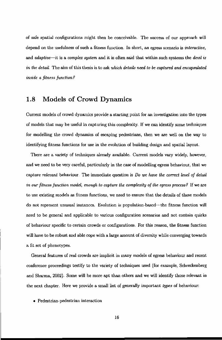
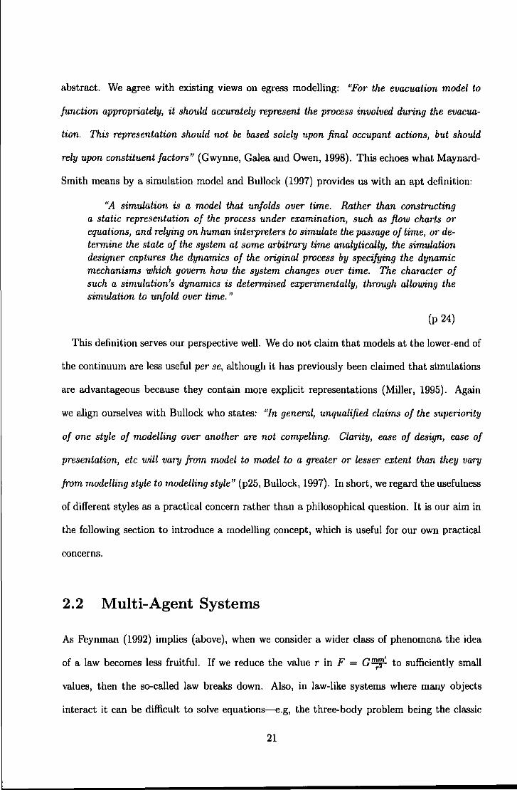
Figure 2.1: A simple example of emergent behaviour. Wood chips are collected over time into larger and larger piles due to the feedback created in the environment rather than an explicit woodchip-collecting rule. Adapted from R.esnick (1994).

of a computational model, t his sounds like good news for the computer scientist-complex

behaviour need not necessarily demand the implementation of a correspondingly complex rep-

resentation.

2.2.2 Virtual MAS

Indeed, some of the early models in the field of A-Life demonstrate this idea. For example,

in natural systems, animals appear to flock for reasons related to survival (e.g., herding prey)

or perhaps to minimise energy (e.g., birds slip-streaming in flight). When we observe a flock

of birds invisible hands appear to orchestrate cooperative and complex movement. However,

for virtual flocking to occur three simple rules suffice: 1) Move within a certain distance of

neighbours, 2) Match velocity with neighbours 3) Prevent collision by limiting the effect of rule

1. These local rules, executed in agents called 'boids', produce satisfyingly complex flocking

behaviour (Reynolds, 1987).

Another example is Resnick's (1994) virtual termite wood- piling model. Here, termites live

on a two dimensional lattice and follow two rules: 1) If encounter wood-chip, then pick-up

wood-chip; 2) If carrying wood-chip and encounter wood-chip, then drop wood-chip. With

random wood-chip initialisation and random termite movement scattered chips are accumu-

lated into large piles. We present example epochs of termite behaviour (see Figure 2.1) .

These kinds of patterns are often referred to as emergent because they are not represented

23

explicitly in model rules. In the recent past, such algorithms have produced much excite-

ment, but more recently, experts have pointed out reasons for the apparent lack of success of

Distributed Intelligence and in particular the lack of application. AB Bonabeau, Dorigo and

Theraulaz (1999) state:

"It is fair to say that very few applications of swarm intelligence have been developed. Swarm-intelligent systems are hard to "progro.m", because the paths to problem solving are not pre-defined, but emergent in these systems and result from intemctions among individuals and between individuals and their environment as much as from the behaviour of the individuals themselves. Therefore, using a swarm-intelligent system to solve a problem requires a thorough knowledge, not only of what individual behaviours must be implemented but also of what intemctions are needed to produce such or such global behaviour. "

(p 7)

The clear message is that we need to represent the behaviours of single entities well to

successfully exploit emergence. Although it might be possible to implement simple rules to

produce system-level behaviour, the difficulty is in uncovering the appropriate rules.

2.2.3 Pedestrian MAS

In a similar way to ants in nests and birds in flocks, pedestrians can be thought of as the units

or agents in a pedestrian crowd. Most of the time pedestrians co-operate and crowds show

unproblematic, well-structured, predictable behaviour. However, there are situations where

actions produce unintended consequences because of long chains of interdependence between

pedestrian units. For example, it has been known for a long time that decisions made at

local points in space and time can have effects that result in blockages, areas of very densely

packed pedestrians, which may result in injury or death (Canter, 1980). In a similar way to

the natural and virtual systems above, local actions generate global behaviour.

Individuals within the system act interactively with respect to local circumstances and,

as Bonabeau et al. (1999) suggest, it is the interaction between pedestrians and between

pedestrians and their environment, which presents the main challenge from a modelling point

of view. In an extensive review of real human behaviour in egress situations a number of

24

attributes have been identified (Gwynne et al., 1998). We give a general summary of some of

them here, encapsulated by the three broad classes of interactions given in chapter 1.

• Pedestrian-pedestrian intemction: This describes the culmination of interactions be

tween individuals as they escape. Local and global decisions are important-rather than

blindly follow a given direction of egress, individuals seem to act adaptively and update

decisions according to changing circumstances. Pedestrians also co-operate and demon

strate group behaviour. One widely cited example is the appearance of lane formations,

which optimise crowd-flow (Helbing, Farkas, Molnr and Vicsek, 2002). However, pedes

trians also show conflicting behaviour, and where flow becomes viscous blockages result

in injury.

• Pedestrian-environment intemction: This refers to the direct physical impact of an

enclosure upon occupants. Design decisions not only include building structure, but

crucial elements are the position of exit signs and the travel distance from a given

location in the building to an escape exit. Pedestrian reactions to the environment

impinge on how pedestrians interact with each other. Also, pedestrians show a range of

navigation ability in dynamic environments.

• Adaptive escape behaviour: Observations indicate that the huge majority of individuals

react in an adaptive, decision-making manner, rather than by default to some herding

instinct (a common assumption often made in the past). It is argued that theories based

on a herding instinct are rather the default reactions of some scientists to behaviours

that have not been well understood.

There are a wide variety of modelling techniques used, which capture some of these prop

erties to varying degrees. Some approaches can be classified as MAS and others maybe not.

We begin with approaches that utilise a discrete representation of space.

25

2.3 Discrete Models

2.3.1 Discrete Space

With discrete space there cannot be an infinite number of spatial fragments as opposed to

continuous space where any given fragment is itself infinitely divisible. Lets consider Zeno's

paradox (Huggert, 1999):

"Imagine our runner-her name is Atlanta-bursting over a starting line and hurtling towards the finish at top speed. First, she must tmvel half the distance, namely 50m, leaving 50m to go. Then half the remaining distance, 50m72=25m and so on... There is no end to the number of times we can halve the remaining distance; hence Atlanta must cover an infinite number of finite distances to get to the finish".

(p 39)

With discrete space we choose an a-priori spatial unit and have to stick to it. Then any

operation that divides this unit is deemed invalid. Therefore Zeno's paradox cannot occur

in discrete space-Atlanta's movement cannot. divide a prcdefined quantity. If we use this

quantity as the lowest limit of movement, then Atlanta will pass the finish line at some point

in time, rather than never. In the same way, if a pedestrian will move in a given period of

time, then it will move at least one unit or an integer multiple of this unit.

There is no rule stating that the unit chosen should be a certain size, but once this is chosen

it it is chosen. The following set of discrete models depend on different choices in this respect

and these choices introduce specific properties to the model.

2.3.2 Coarse Network Representations

2.3.2.1 Graphs (briefly)

The network approach uses the language of Graph Theory where vertices and edges are the

basic units of representation. A vertex represents some abstract object, e.g., a person or

an area of land. An edge is an abstract relationship or interaction between one object and

another. A Graph represents the intemction network; it consists of the entire set of objects

26

t(1

An~elo Benoit •• 1~ 1

~· Chaz Dave

Chaz(C)

Augelo~D•ve(DJ Beuoit(B)

/"

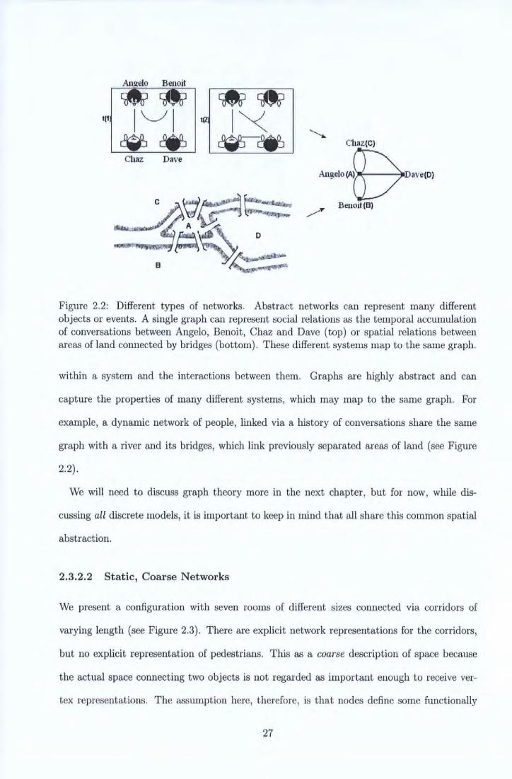
Figure 2.2: Different types of networks. Abstract networks can represent many different objects or events. A single graph can represent social relations as the temporal accumulation of conversations between Angelo, Benoit, Chaz and Dave (top) or spatial relations between areas of land connected by bridges (bottom). These different systems map to the same graph.

within a system and the interactions between them. Graphs are highly abstract and can

capture the properties of many different systems, which may map to the same graph. For

example, a dynamic network of people, linked via a history of conversations share the same

graph with a river and its bridges, which link previously separated areas of land (see Figure

2.2) .

We will need to discuss graph theory more in the next chapter, but for now, while dis-

cussing all discrete models, it is important to keep in mind that all share this common spatial

abstraction.

2.3.2.2 Static, Coarse Networks

'Ne present a configuration with seven rooms of different sizes connected via corridors of

varying length (see Figure 2.3). There are explicit network representations for the corridors,

but no explicit representation of pedestrians. This as a coarse description of space because

the actual space connecting two objects is not regarded as important enough to receive ver-

tex representations. The assumption here, therefore, is that nodes define some functionally

27

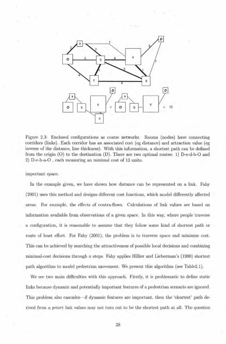
13

Figure 2.3: Enclosed configurations as coarse networks. Rooms (nodes) have connecting corridors (links). Each corridor has an associated cost ( eg distance) and at traction value ( eg inverse of the distance, line thickness). With this information, a shortest path can be defined from the origin (0) to the destination (D). There are two optimal routes: 1) D-e-d-b-0 and 2) D-e-b-a--0 , each measuring an minimal cost of 13 units.

important space.

In the example given, we have shown how distance can be represented on a link. Fahy

(2001) uses this method and designs different cost functions, which model differently affected

areas. For example, the effects of contra-flows. Calculations of link values are based on

information available from observations of a given space. In this way, where people traverse

a configuration, it is reasonable to assume that they follow some kind of shortest path or

route of least effort. For Fahy (2001) , the problem is to traverse space and minimise cost.

This can be achieved by searching the attractiveness of possible local decisions and combining

minimal-cost decisions through n steps. Fal1y applies Hillier and Lieberrnan's (1990) shortest

path algorithm to model pedestrian movement. We present t his algorithm (see Table2.1).

We see two main difficulties with this approach. Firstly, it is problemat ic to define static

links because dynamic and potentially important features of a pedestrian scenario are ignored.

This problem also cascades-if dynamic features are important, then the 'shortest' path de-

rived from a priori link values may not turn out to be the shortest path at all. The question

28

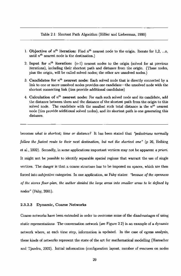
Table 2.1: Shortest Path Algorithm (Hillier and Lieberman, 1990)

1. Objective of nth iteration: Find nth nearest node to the origin. Iterate for 1,2, ... n, until nth nearest node is the destination.)

2. Input for nth iteration: (n-1) nearest nodes to the origin (solved for at previous iterations), including their shortest path and distance from the origin. (These nodes, plus the origin, will be called solved nodes; the other are unsolved nodes.)

3. Candidates for nth nearest node: Each solved node that is directly connected by a link to one or more unsolved nodes provides one candidate-the unsolved node with the shortest connecting link (ties provide additional candidates)

4. Calculation of nth nearest node: For each such solved node and its candidate, add the distance between them and the distance of the shortest path from the origin to this solved node. The candidate with the smallest such total distance is the nth nearest node (ties provide additional solved nodes), and its shortest path is one generating this distance.

becomes what is shortest; time or distance? It has been stated that "pedestrians normally

follow the fastest route to their next destination, but not the shortest one" (p 26, Helbing

et al., 2002). Secondly, in some applications important vertices may not be apparent a priori.

It might not be possible to identify separable spatial regions that warrant the use of single

vertices. The danger is that a coarse structure has to be imposed on spaces, which are then

forced into subjective categories. In one application, as Fahy states: "because of the openness

of the stores floor-plan, the author divided the large areas into smaller areas to be defined by

nodes" (Fahy, 2001).

2.3.2.3 Dynamic, Coarse Networks

Coarse networks have been extended in order to overcome some of the disadvantages of using

static representations. The conversation network (see Figure 2.2) is an example of a dynamic

network where, at each time step, information is updated. In the case of egress analysis,

these kinds of networks represent the state of the art for mathematical modelling (Hamacher

and Tjandra, 2002). Initial information (configuration layout, number of evacuees on nodes

29

etc ... ) is processed and updated, providing input for the next iteration on the graph. The

graph at the next iteration therefore has the same topology, but different, updated vertices

and edge values. The resulting network is, therefore, a temporal expansion of the former kind

and attempt to capture the dynamic features of escape behaviour.

However, important detail is minimally represented in these models, if at all. Measures

such as distances and costs need to be known a-priori, based on manual measurements of

a given configuration. This is not a disadvantage for a specific application, because time

can be spent making these measurements, but when we want to execute a model in any given

configuration, this information may not be known. Tltis is particularly true if the configuration

is to be generated automatically by some kind of algorithm 2•

This thesis is concerned with using a general egress model, which is capable of representing

the detailed pedestrian-pedestrian and pedestrian-environment interactions. This detail is not

adequately represented in either coarse-static or coarse-dynamic networks. If we are to use a

model as a fitness function within an evolutionary context, then we need explicit representation

of these fine-grained details.

It is only relatively recently that available computer power has enabled the implementation

of such detail. The next section introduces agent-based approaches, wltich operate on finer

grained networks.

2.3.3 Fine Network Representations

Here we briefly introduce three examples, which utilise a fine-grained network. Not all of them

are directly related to egress analysis, but represent general techniques relevant for modelling

movement in arbitrarily complex, labyrinthine space.

EXODUS: This is an example of a commercially available software package with a 3-D

graphical user-interface, but some of the underlying methods are familiar. The un

derlying representation of space is two-dimensional. Unlike the approaches outlined

2We will return to the automatic generation of space later on in the thesis (Chapter 7).

30

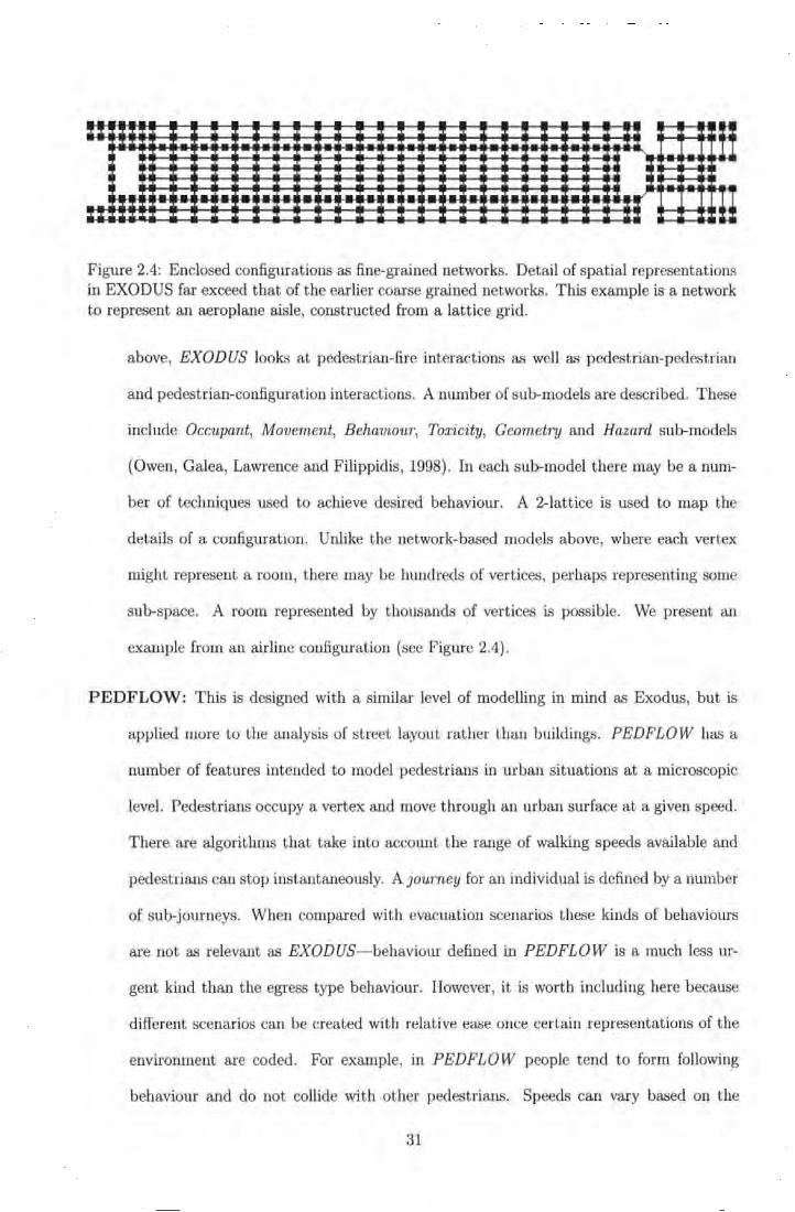
-- ·-- -- :n ::z:::z: :::z: :I :I -- ·- ·- ·- ·- - ·- ·- ••• ....... ; ·- - ·--·-- ,. ·- - - - - - ·- ·- ,.

1 .• ,. ,. .• ,_ ,. ·- ,. ,. ,. , • ..1' :H -- ;;;~;;;~; • •

Figure 2.4: Enclosed configurations as fine-grained networks. Detail of spatial representations in EXODUS far exceed that of the earlier coarse grained networks. This example is a network to represent an aeroplane aisle, constructed from a lattice grid.

above, EXODUS looks at pedestrian-fire interactions as well as pedestrian-pedestrian

and pedestrian-configuration interactions. A number of sub-models are described. These

include Occupant, Movement, Behaviour, Toxicity, Geometry and Hazard sub-models

(Owen, Galea, Lawrence and Filippidis, 1998). In each sub-model there may be anum-

ber of techniques used to achieve desired behaviour. A 2-lattice is used to map the

details of a configuration. Unlike the network-based models above, where each vertex

might represent a room, there may be hundreds of vertices, perhaps representing some

sub-space. A room represented by thousands of vertices is possible. We present an

example from an airline configuration (see Figure 2.4).

PEDFLOW: This is designed with a similar level of modelling in mind as Exodus, but is

applied more to the analysis of street layout rather than buildings. PEDFLOW has a

nwnber of features intended to model pedestrians in urban situations at a microscopic

level. Pedestrians occupy a vertex and move through an urban surface at a given speed.

There are algorithms that take into account the range of walking speeds available and

pedestrians can stop instantaneously. A journey for an individual is defined by a number

of sub-journeys. When compared with evacuation scenarios these kinds of behaviours

are not as relevant as EXODUS- behaviour defined in PEDFLOW is a much less ur-

gent kind than the egress type behaviour. However, it is worth including here because

different scenarios can be created with relative ease once certain representations of the

environment are coded. For example, in PEDFLOW people tend to form following

behaviour and do not collide with other pedestrians. Speeds can vary based on the

31

'urgency' of the journey and pedestrians also avoid obstacles. These behaviours are very

similar to the ones defined in EXODUS. In addition, PEDFLOW incorporates models

of traffic flow into the urban environment so that the interaction of 'pedestrian' and

'traffic' models can be analysed (Jones, 1996; Kerridge, 2001).

STREETS: This is developed in The Centre for Advanced Spatial Analysis at University

College London. It also has the aim of analysing pedestrian behaviour in the built urban

environment. Again, although not directly relevant to egress behaviour, the model uses

conunon techniques and a fine-grained representation of space. A particular application

is the Notting Hill Carnival (Batty, DeSyllas and Duxbury, 2002).

Like PEDFLOW, pedestrians are given a journey and can stop at various positions to·

complete 'sub-tasks' on their way. Pedestrians follow simple rules to produce behaviours-

avoidance of other agents and navigation around representations of buildings. Pedes-

trians follow street layout on their way to a globally defined destination. There are no

generally defined, computational behaviours in such a model. Behaviour will be defined

based on observations of real crowds at the application event because the software is

developed in the context of real applications. One advantage of this is that the model

can be evaluated against data collected from real events. This is important for model

calibration (Gwynne et al., 1998). However, the downside is that the algorithms are less

generally applicable to other scenarios.

Publications point towards the relevance of Cellular Automata approaches (Torrens,

2000) used to model populations moving through streets. A map of street-layout is

developed and the surface are created by the use of a stigmergy-based algorithm3 . Sue-

cessful pedestrians deposit attraction forces that decay over time (Batty et al., 2002).

The build up of this dynamic quantity makes some areas more attractive than others and

the model then behaves in a way that simulates crowding behaviour as attractors are

3 BrciHy, stigmergy refers to interactive feedback between a.n agent a.nd its environment. Pheromone interaction in a.nts (see above) is one example.

32

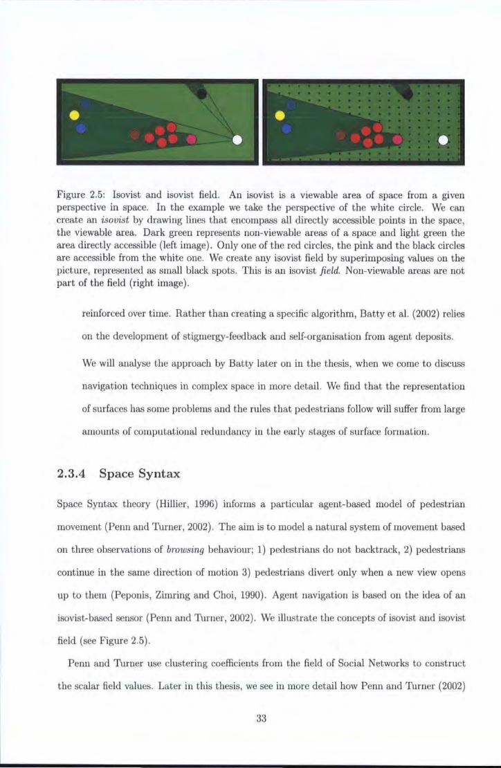
Figure 2.5: Isovist and isovist field. An isovist is a viewable area of space from a given perspective in space. In the example we take the perspective of the white circle. We can create an isovist by drawing lines that encompass all directly accessible points in the space, the viewable area. Dark green represents non-viewable areas of a space and light green the area directly accessible (left image). Only one of the red circles, the pink and the black circles are accessible from the white one. We create any isovist field by superimposing values on the picture, represented as small black spots. This is an isovist field. Non-viewable areas are not part of the field (right image).

reinforced over time. Rather than creating a specific algorithm, Batty et al. (2002) relies

on the development of stigmergy-feedback and self-organisation from agent deposits.

We will analyse the approach by Batty later on in the thesis, when we come to discuss

navigation techniques in complex space in more detai l. We find that the representation

of surfaces has some problems and the rules that pedestrians follow will suffer from large

amounts of computational redundancy in the early stages of surface formation.

2.3.4 Space Syntax

Space Syntax theory (Hillier, 1996) informs a particular agent-based model of pedestrian

movement (Penn and Turner, 2002). The aim is to model a natural system of movement based

on three observations of browsing behaviour; 1) pedestrians do not backtrack, 2) pedestrians

continue in the same direction of motion 3) pedestrians d ivert only when a new view opens

up to them (Peponis, Zimring and Choi, 1990). Agent navigation is based on the idea of an

isovist-based sensor (Penn and Thrner, 2002). We illustrate the concepts of isovist and isovist

field (see Figure 2.5).

Penn and Turner use clustering coefficients from the field of Social Networks to construct

the scalar field values. Later in this thesis, we see in more detail how Penn and Turner (2002)

33

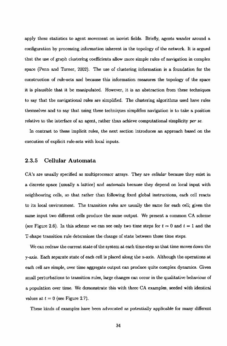
apply these statistics to agent movement on isovist fields. Briefly, agents wander around a

configuration by processing information inherent in the topology of the network. It is argued

that the use of graph clustering coefficients allow more simple rules of navigation in complex

space (Penn and Thrner, 2002). The use of clustering information is a foundation for the

construction of rule-sets and because this information measures the topology of the space

it is plausible that it be manipulated. However, it is an abstraction from these techniques

to say that the navigational rules are simplified. The clustering algorithms used have rules

themselves and to say that using these techniques simplifies navigation is to take a position

relative to the interface of an agent, rather than achieve computational simplicity per se.

In contrast to these implicit rules, the next section introduces an approach based on the

execution of explicit rule-sets with local inputs.

2.3.5 Cellular Automata

CA's are usually specified as multiprocessor arrays. They are cellular because they exist in

a discrete space (usually a lattice) and automata because they depend on local input with

neighbouring cells, so that rather than following fixed global instructions, each cell reacts

to its local environment. The transition rules are usually the same for each cell; given the

same input two different cells produce the same output. We present a common CA scheme

(see Figure 2.6). In this scheme we can see only two time steps for t = 0 and t = 1 and the

T-shape transition rule determines the change of state between these time steps.

We can redraw the current state of the system at each time-step so that time moves down the

y-axis. Each separate state of each cell is placed along the x-axis. Although the operations at

each cell are simple, over time aggregate output can produce quite complex dynamics. Given

small perturbations to transition rules, large changes can occur in the qualitative behaviour of

a population over time. We demonstrate this with three CA examples, seeded with identical

values at t = 0 (see Figure 2.7).

These kinds of examples have been advocated as potentially applicable for many different

34

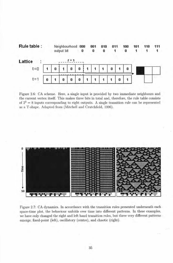
Rule table:

Lattice

t=O

t =1

1

0

Neighbourhood : ooo 001 010 011 output bit 0 0 0 1

r=1

0 1

1 0

100 101 110 111 0 1 1 1

0

1

Figure 2.6: CA scheme. Here, a single input is provided by two immediate neighbours and the cmrent vertex itself. This makes three bits in total and, therefore, the rule table consists of 23 = 8 inputs corresponding to eight outputs. A single transition rule can be represented as aT-shape. Adapted from (Mitchell and Crutchfield, 1996).

0

(I)

E

l 50

Figure 2.7: CA dynamics. In accordance with the transit ion rules presented underneath each space-time plot, the behaviour unfolds over time into different patterns. In these examples, we have only changed the right and left hand transition rules, but three very different patterns emerge; fixed-point (left), oscillatory (centre), and chaotic (right).

35

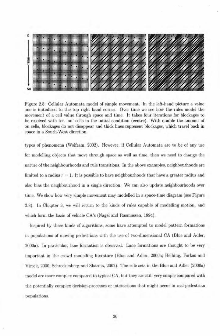
0

Cl)

,;

1 Figure 2.8: Cellular Automata model of simple movement. In the left-hand picture a value one is initialised to the top right hand corner. Over time we see how the rules model the movement of a cell value through space and time. It takes four iterations for blockages to be resolved with ten 'on' cells in the initial condition (centre). With double the amount of on cells, blockages do not disappear and thick lines represent blockages, which travel back in space in a South-West direction.

types of phenomena (Wolfram, 2002). However, if Cellular Automata are to be of any use

for modelling objects that move through space as well as time, then we need to change the

nature of the neighbourhoods and rule transitions. In the above examples, neighbourhoods are

limited to a radius r = 1. It is possible to have neighbourhoods that have a greater radius and

also bias the neighbourhood in a single direction. We can also update neighbourhoods over

time. We show how very simple movement may modelled in a space-time diagram (see Figure

2.8). In Chapter 3, we will return to the kinds of rules capable of modelling motion, and

which form the basis of vehicle CA's (Nagel and Rasmussen, 1994).

Inspired by these kinds of algorithms, some have attempted to model pattern formations

in populations of moving pedestrians with t he use of two-dimensional CA {Blue and Adler,

2000a). In particular, lane formation is observed. Lane formations are thought to be very

important in the crowd modelling literature (Blue and Adler, 2000a; Helbing, Farkas and

Vicsek, 2000; Schreckenberg and Sharma, 2002) . The rule sets in the Blue and Adler {2000a)

model are more complex compared to typical CA, but they are still very simple compared with

the potentially complex decision-processes or interactions that might occur in real pedestrian

populations.

36

It might be argued that the simplicity of these programs might urge us to classify them at the

lower end of the modelling continuum. However, the important properties of cellular automata

are that they are developmental and supposedly elicit self-organisation. For example, it is

shown that from a random, initial configuration, behaviour will not organise until around one

hundred time-steps into the simulation, which illustrates the emergent nature of this approach

(Blue and Adler, 2000a}.

In the next chapter we will provide a more technical review of some of the discrete models,

which represent individuals, crowds and configurations. Firstly, we will review models based

on a continuous concept of space.

2.4 Continuous Models

2.4.1 Continuous Space

With Zeno's paradox, we know there is a problem in the reasoning. It was used to illustrate the

concept of discrete space as consisting of an indivisible unit. What is wrong with the paradox?

As Feynman states: " ... a finite amount of time can be divided into a infinite number of pieces

just as the length of a line can be divided into an infinite number of pieces by dividing it by

two" (Feynman, 1963). In other words Zeno ignores the time dimension.

Infinitesimal distance must be coupled with infinitesimal time, so that distance coverage

occurs in the spatial and temporal domain. We can then find the ratio of this coupling when

a change in time approaches zero. This ratio we call velocity v:

I. tJ.s

v= 1m T .:lot--+11 u.t (2.2)

This infinite fragmentation of distance according to time is common to some of the con-

tinuous approaches below, which calculate a quantity of spatial movement from local forces

without having to impose it beforehand.

37

2.4.2 Fluid Dynamics

It is clear to see how fluid dynamic-based approaches have been used in the study of crowd

ing people. Fluid is a tempting analogy, because it moves through space and avoids obsta

cles. Applications of this approach have been applied to various problems (Smith and Dick

1993), but are often limited to situations where the density of the crowd is relatively high

(Hughes, 2002; Hughes, 2003). The assumption is that the crowd is like a fluid at high den

sity, because the choices that people make are more constrained by the choices of others. As

crowd density increases each person has reduced freedom. Reactions become less like a collec

tion of individuals and more like a single, fully connected mass, just like separable particles

made of hydrogen and oxygen atoms attract to form the collective we call 'water'.

These kinds of assumptions underpin methods in the fluid dynamics approach. Applications

of this approach are therefore limited to situations with large amounts of people (Hughes,

2002). Hughes' equations can model a homogenous population, where speed is assumed to be a

function of total density. This is a particularly unrealistic assumption, but the maths gets very

complex and tractable analysis requires populations to be handled en mass (Hughes, 2002).

The fluid analogy has been criticised and more granular approaches advocated (Still, 2000).

Still argues that the underlying assumption, (flow volume = average speed x average density),

is simply too unrealistic when compared to complexities in real crowds. The assumptions

underneath the fluid analogy are questionable and the failure of these models to produce

sensible behaviours at low densities is a severe drawback.

In the current thesis it will be desirable to have a model represent populations of varying

densities, both between different configurations, but also within a configuration. It is well

observed that in egress situations some parts of the population can move freely, whereas others

form blockages. A real population is heterogeneous, unlike water, and rules of movement need

to incorporate density fluctuations. Ideally, a model should remain robust to the density

parameter.

38

2.4.3 Steering Dynamics

Apart from flocking behaviour in 'boids', Reynolds has developed steering behaviours for

autonomous characters in an environment (Reynolds, 1999). The motivation for Reynolds

is to create characters in games that are autonomous and react to varying environmental

conditions. The aim is to produce more natural behaviour and his work has Strong Artificial

Life overtones; "real agents in a virtual world" (Reynolds, 1999). Steve Grand shares similar

views and warns against attempts to interpret outward behavioural rules by advocating the

use of Newtonian mechanics: " ... they should be trying to model Newton's basic equations of

motion and the curves would turn up all by themselves, complete with swerving, skidding and

all the other things that help convince people" (p73, Grand, 2000).

Reynolds attempts to model movement by designing mechanical devices that work at a

local level. He defines three levels to the autonomous characters; locomotion, steering and

action selection. The locomotion layer is defined as a simple vehicle in the sense meant by

(Braitenberg, 1984) and is essentially a point mass with various scalar and vector quantities to

describe mass, position and orientation. Steering is simulated by a velocity aligned local space,

where incremental adjustments are made on the previous time step to a current velocity vector

and a desired velocity vector. We can see that an agent floats in two dimensions (see Figure

2.9), a very different way of modelling motion compared with the lattice-based approaches in

Section 2.3.

2.4.4 Social Dynamics

One attempt has been made to apply Newtonian mechanics to moving populations of esca~

ing people, whose vectors represent various desires and constraints in the context of egress

behaviour (Helbing et al., 2000; Helbing, Farkas and Vicsek, 2001; Helbing et al., 2002).

To model how a crowd of people move through space over time a mathematical theory using

differential calculus must be able to 1) describe the changes in positions of individuals and 2)

have some method of recording these changes so that behaviour unfolds dynamically, moment

39

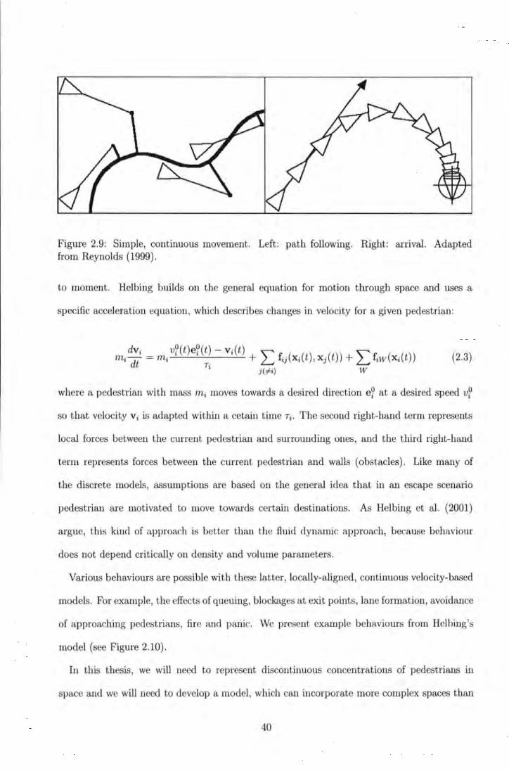
Figure 2.9: Simple, continuous movement. Left: path following. Right: arrival. Adapted from Reynolds (1999).

to moment. Helbing builds on the general equation for motion through space and uses a

specific acceleration equation, which describes changes in velocity for a given pedestrian:

(2.3)

where a pedestrian with mass m; moves towards a desired direction e? at a desired speed v?

so that velocity v; is adapted within a cetain timeT;. The second right-hand term represents

local forces between the current pedestrian and surrounding ones, and the third right-hand

term represents forces between the current pedestrian and walls (obstacles). Like many of

the djscrete models, assumptions are based on the general idea that in an escape scenario

pedestrian are motivated to move towards certain destinations. As Helbing et al. (2001)

argue, this kind of approach is better than the fluid dynamic approach, because behaviour

does not depend critically on density and volume parameters.

Various behaviours are possible with these latter, locally-aligned, continuous velocity-based

models. For example, the effects of queuing, blockages at exit points, lane formation, avoidance

of approaching pedestrians, fire and panic. We present example behaviours from Hclbing's

model (see Figure 2.10).

In this thesis, we will need to represent discontinuous concentrations of pedestrians in

space and we will need to develop a model, which can incorporate more complex spaces than

40

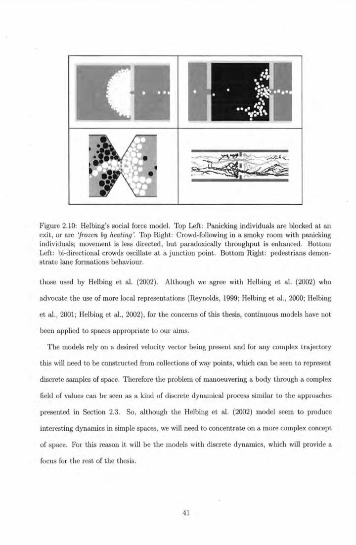
Figure 2.10: Helbing's social force model. Top Left: Panicking individuals are blocked at an exit, or are 'frozen by heating'. Top Right: Crowd-following in a smoky room with panicking individuals; movement is less directed, but paradoxically throughput is enhanced. Bottom Left: bi-directional crowds oscillate at a junction point. Bottom Right: pedestrians demonstrate lane formations behaviour.

those used by Helbing et al. (2002) . Although we agree with Helbing et al. (2002) who

advocate the use of more local representations (Reynolds, 1999; Helbing et al., 2000; Helbing

et al., 2001; Helbing et al. , 2002), for the concerns of this thesis, continuous models have not

been applied to spaces appropriate to our aims.

The models rely on a desired velocity vector being present and for any complex trajectory

this will need to be constructed from collections of way points, which can be seen to represent

discrete samples of space. Therefore the problem of manoeuvering a body through a complex

fie ld of values can be seen as a kind of discrete dynamical process similar to the approaches

presented in Section 2.3. So, although the Helbing et al. (2002) model seem to produce

interesting dynamics in simple spaces, we will need to concentrate on a more complex concept

of space. For this reason it will be the models with discrete dynamics, which will provide a

focus for the rest of the thesis.

41

2.5 Summary

In this chapter we:

• identified with the idea of a modelling continuum.

- Models are domain specific and serve different purposes. We found the distinction

between simple models and simulation models useful.

• introduced pedestrian crowds as Multi-Agent Systems (MAS).

- This concept can be thought of as key in the design of simulation models; it can

encompass the processes of egress behaviour at an appropriate level of abstraction.

• critically reviewed a number of discrete approaches

- Coarse network representations do not provide a detailed enough representation of

pedestrian crowds, which in light of the current thesis is a severe limitation.

- Fine network representations are more appropriate methods in the light of the

MAS concept. These finer-grained approaches use the concept of an attractor field

in order to model long-range movement.

- Cellular Automata represent local pedestrian decisions and interactions with simple

rules. Such rules lead to important emergent properties found in real crowds, such

as lane formations.

• reviewed continuous approaches

- Although this approach looks like a promising technique, in such models the notion

of a configuration is rather underdeveloped and inappropriate in the broader context

of this thesis.

42

Having narrowed down the potential use of wide-ranging techniques, we now begin to con

centrate on 2 kinds of discrete model. We focus on techniques- attractor fields and Cellular

Automata- which model long-range movement and local dynamics, respectively.

43

Chapter 3

Pedestrian and Evacuation Dynamics

11

Firstly, we outline some technical detail. Because graphs underpin discrete models of pedes

trian and evacuation dynamics, we familiarise ourselves with Graph definitions and graph

walks (see Section 3.1). We look at two relevant applications of Graph Theory and the sta

tistical techniques used to capture spatial relationships (see Section 3.2).

Secondly, having provided a technical background, we then critique discrete models of pedes

trian and evacuation dynamics in the context of thesis aims (see Section 3.3). This critique will

lead to a clear view of which methods need more fine-grained investigations. The summary

at the end of the chapter clarifies our arguments (see Section 3.3).

3.1 Graph Theory

3.1.1 Graphs

In order that we can properly review discrete models of pedestrian movement, we need to

know what their underlying space is made of. The following definitions are important for

the rest of the thesis and, in accordance with the following definitions, we present examples

44

(see Figure 3.1). 1

Definition 1 A graph G contains a set of vertices V( G) together with a set of vertex pairs

called edges E(G). The number of elements IV(G)j and jE(G)j are known as the order and

size of G, respectively.

Definition 2 The global structure of G is important-a graph is connected if any vertex is

reachable from any other, otherwise it is disconnected. Connected graphs are therefore referred

to as single-component whereas disconnected graphs are described as multi-component.

Definition 3 A simple graph is an undirected graph where edges provide no specific repre-

sentation for direction. For example, if we consider networks like the examples in Chapter 2

(see Figure 2.2), then undirected means that two people talk to each other, or a bridge can be

crossed from either side. In this way, the objects are connected in a bi-directional relationship.

Definition 4 The number of edges shared by a given vertex v is the degree kv.

Definition 5 The degree of v is related to its neighbourhood r v, which is a set of vertices not

containing v, but sharing an edge with it.

Definition 6 We refer toad-lattice as a case where any vertex vis joined to lattice neighbours

throughout the entire graph of dimension d. In models of pedestrian and evacuation dynamics,

the d-lattice representation is common, in particular where d = 2. However, d = 1 is also an

important kind of lattice2.

Definition 7 A d-lattice has boundaries, which can either be periodic or non-periodic. 'Peri-

odic' refers to a lattice, which is said to be 'wrapped-around', where the pattern of connectivity

applies to the entire graph. A 'non-periodic' lattice is where vertices have heterogeneous neigh-

bourhood structure. For example, boundary vertices may connect with fewer neighbours than

is typical of the rest of the lattice and thus periodic structures are broken.

1These definitions are based on Watts (1999) and Wilson (1985). 2This will become apparent when we consider in more detail the relationship between the Vehicle Cellular

Automata (Nagel and Rasmussen, 1994) and the pedestrian Cellular Automata (Blue and Adler, 2000a). See Chapter 4.

45

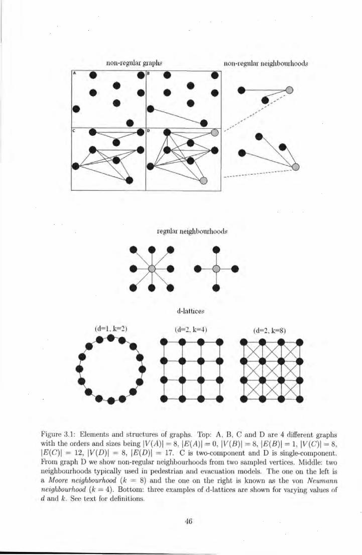
A

• • •

non-regular p:rnphs

• •

• non-regular neighbourhoods

• ' '

__ yo ---

regular neighbourhood:>

d-lattices

Cd=l , 1:-:n (d=2. k--n (d=:!, 1:=8)

Figure 3.1: Elements and structures of graphs. Top: A, B, C and D are 4 di fferent graphs with the orders and sizes being IV(A)I = 8, IE(A)I = 0, IV(B)I = 8, IE(B)I = 1, IV(C)I = 8, IE(C)I = 12, IV(D)I = 8, IE(D)I = 17. C is two-component and D is single-component. From graph D we show non-regular neighbourhoods from two sampled vertices. Middle: two neighbourhoods typically used in pedestrian and evacuation models. The one on the left is a Moore neighbourhood (k = 8) and the one on t he right is known as the van Neumann neighbourhood (k = 4). Bottom: three examples of cl-lattices are shown for varying values of d and k. See text for definitions.

46

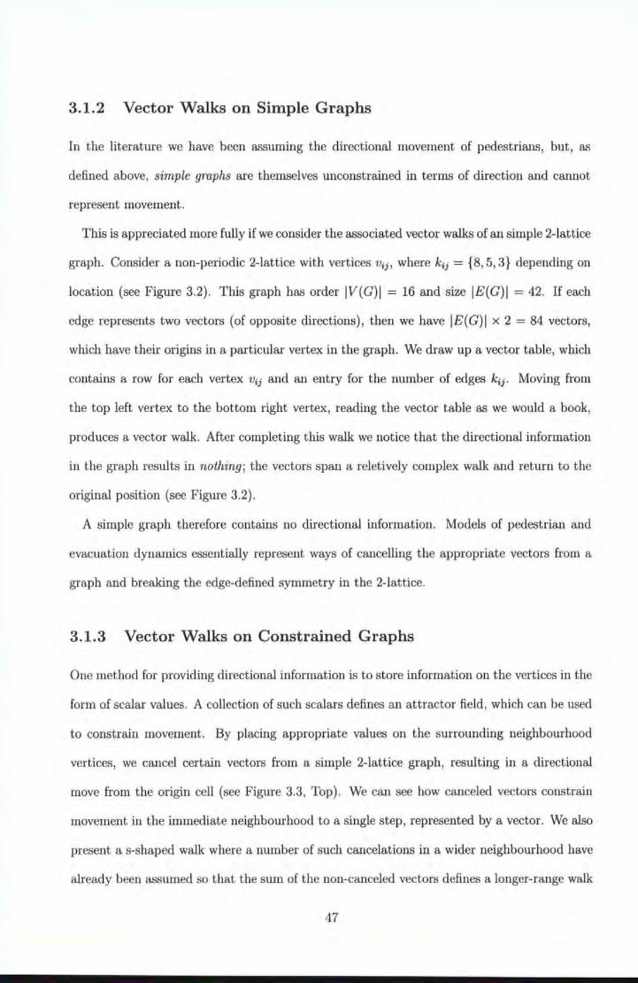
3.1.2 Vector Walks on Simple Graphs

In the literature we have been assuming the directional movement of pedestrians, but, as

defined above, simple graphs are themselves unconstrained in terms of direction and cannot

represent movement.

This is appreciated more fully if we consider the associated vector walks of an simple 2-lattice

graph. Consider a non-periodic 2-lattice with vertices Vij , where kii = {8, 5, 3} depending on

location (see Figure 3.2). This graph has order IV(G)I = 16 and size IE(G)I = 42. If each

edge represents two vectors (of opposite directions) , then we have IE(G)I x 2 = 84 vectors,

which have their origins in a particular vertex in the graph. We draw up a vector table, which

contains a row for each vertex vii and an entry for the number of edges kii. Moving from

the top left vertex to the bottom right vertex, reading the vector table as we would a book,

produces a vector walk. After completing this walk we notice that the directional information

in the graph results in nothing; the vectors span a reletively complex walk and return to the

original position (see Figure 3.2).

A simple graph therefore contains no directional information. Models of pedestrian and

evacuation dynamics essentially represent ways of cancelling the appropriate vectors from a

graph and breaking the edge-defined symmetry in the 2-lattice.

3.1.3 Vector Walks on Constrained Graphs

One method for providing directional information is to store information on the vertices in the

form of scalar values. A collection of such scalars defines an attractor field , which can be used

to constrain movement. By placing appropriate values on the surrounding neighbourhood

vertices, we cancel certain vectors from a simple 2-lattice graph, resulting in a directional

move from the origin cell (see Figure 3.3, Top). We can see how canceled vectors constrain

movement in the immediate neighbourhood to a single step, represented by a vector. We also

present a s-shaped walk where a number of such cancelations in a wider neighbourhood have

already been assumed so that the sum of the non-canceled vectors defines a longer-range walk

47

~ +

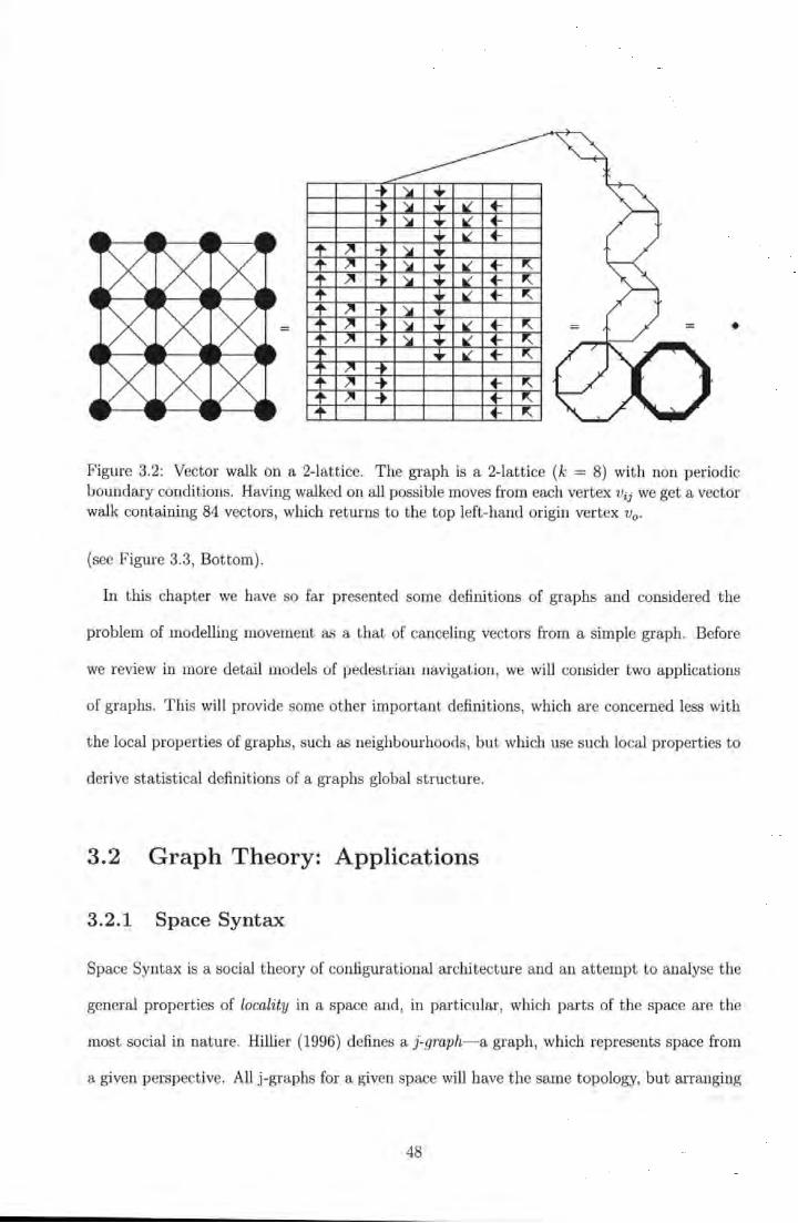
... )f + ... ~ + _1( f-... )f + 11( f-+ _1( f-.,.. ,. ... )f + .,.. ,. ... )f _y_ ~ f- " .,.. ,. ... )f + 11( f- " .,.. ~" 11( f- " .,.. ,. ... )f ~"

= _'t_ ""'

... ~ "'- _f- " = = • .,.. ,. ... )f ~~ 11( f- " er-~ .,.. + 11( f- " ~

""' ....

.... ~ ) .,.. ,. ... f- " .,.. ,. ... f- " .,.. f- " ..........

Figure 3.2: Vector walk on a 2-lattice. The graph is a 2-lattice (k = 8) with non periodic boundary conditions. Having walked on all possible moves from each vertex Vij we get a vector walk containing 84 vectors, which returns to the top left-hand origin vertex v0 •

(see Figure 3.3, Bottom).

In tills chapter we have so far presented some definitions of graphs and considered the

problem of modelling movement as a that of canceling vectors from a simple graph. Before

we review in more detail models of pedestrian navigation, we will consider two applications

of graphs. Tills will provide some other important definitions, which are concerned less with

the local properties of graphs, such as neighbourhoods, but which use such local properties to

derive statistical definitions of a graphs global structure.

3.2 Graph Theory: Applications

3.2.1 Space Syntax

Space Syntax is a social theory of configurational architecture and an attempt to analyse the

general properties of locality in a space and, in particular, which parts of the space are the

most social in nature. Hillier (1996) defines a j-graph- a graph, which represents space from

a given perspective. All j-graphs for a given space will have the same topology, but arranging

48

9 9 11 11

11 10 11 = t 12 10 12 ="'-13 13 13 13

Figure 3.3: Constrained graphs and movement. Top: Constrained von Neumann and Moore neighbours . The neighbourhood represents t he connect ion pattern between nodes, but vertex information defines the allowable moves from a given cell. We show valid (white) and invalid (grey) vectors for the two neighbourhood examples. Movement depends on a minimising option. Bottom: we show a simple s-shaped walk-there can be any number of vector combinations and walks can be more or less complex, but all connect an origin vertex v0 to a destination vertex vd.

the graph in perspective shows how certain areas of space have specific relationships with

other areas in a configuration. With this representation we can see that certain vertices in a

graph are in some sense closer than others to the rest (see Figure 3.4). This idea underpins

the concept of depth, which is a measure of distance.

Definition 8 Given a vertex origin v0 and destination vd we calculate the minimum distance

d(v0 , vd) by traversing an edge subset P(E) . This returns the shortest path between V0 and

vd, or the depth of V 0 from vd, and vice versa. The total vertex depth tvd of V0 is then the

mean shortest path to all other vertices, i.e., we calculate d( V0 , vi )Vj E V and tvd = d.

This is a measure of t he general accessability of vi from vi. A simple one-dimensional space

serves to illustrate this. We choose a 1-lattice space with non-periodic boundaries, which

in the context of a building might represent a corridor. In order to reach some unknown

destination in t his space, it is best to take a position of minimal depth, represented, in our

example, by the centre of the space (see Figure 3.5) .

49

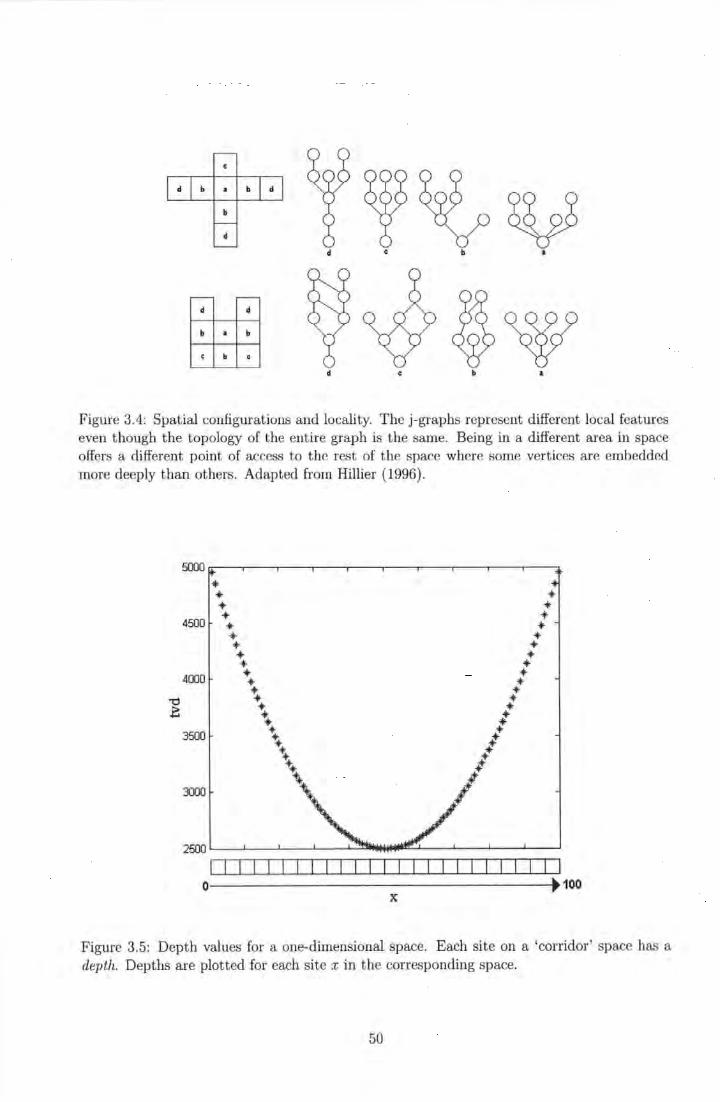
~w d b a

Figure 3.4: Spatial configurations and locality. The j-graphs represent different local features even t hough the topology of the ent ire graph is the same. Being in a different area in space offers a different point of access to the rest of the space where some vert ices are embedded more deeply than others. Adapted from Hillier (1996).

5000

* * * * * * * 4500 * * * .. * * * * * * 4000 * * * * * * ~ * * .e * * \ I

3500 \ l *• I \ I \ ,.,..,

3000 '*-t; ;

" ;

2500

I 0 100

X

Figure 3.5: Depth values for a one-dimensional space. Each site on a 'corridor' space has a depth. Depths are plotted for each site x in t he corresponding space.

50

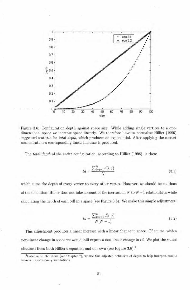
0.9

0.8

0.7

0.6

..r= g. 0.5 "0

0.4

0.3

0.2

0.1

.. .. ······ ....

.. . .. •• ..

•• . . • • . • •

. • . . • .

• . . • .

•

. • .

•

...... ......... 0 ~~~~~-~ ... ~ ... ~---L--~~--~--_L __ _J ____ L_ __ ~

0 10 20 JJ 40 50 size

60 70 80 90 100

Figure 3.6: Configuration depth against space size. While adding single vertices to a onedimensional space we increase space linearly. We therefore have to normalise Hillier (1996) suggested statistic for total depth, which produces an exponential. After applying the correct normalisation a corresponding linear increase is produced.

The total depth of the entire configuration, according to Hillier (1996), is then:

td = ~:j=l d(i,j) N

(3.1)

which sums the depth of every vertex to every other vertex. However, we should be caut ious

of the definition; Hillier does not take account of the increase in N to N - 1 relationships while

calculating the depth of each cell in a space (see Figure 3.6) . We make this simple adjustment:

td = ~:j= L d(i , j) N(N - 1)

(3.2)

This adjustment produces a linear increase with a linear change in space. Of course, with a

non-linear change in space we would still expect a non-linear change in td. We plot t he values

obtained from both Hillier 's equation and our own (see Figure 3.6) .3

3Later ou in t he thesis (see Chapter 7), we use this adjusted definit ion of depth to help interpret results from our evolutionary simulations.

51

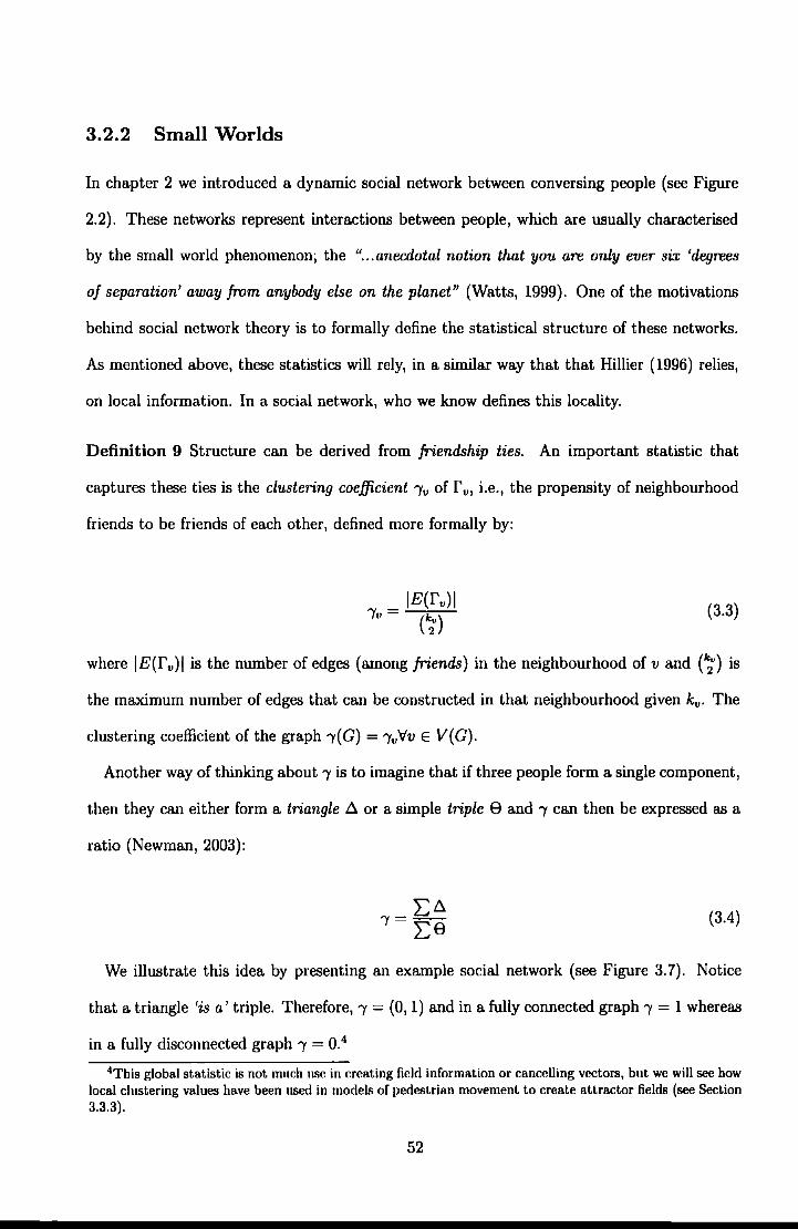
3.2.2 Small Worlds

In chapter 2 we introduced a dynamic social network between conversing people (see Figure

2.2). These networks represent interactions between people, which are usually characterised

by the small world phenomenon; the " ... anecdotal notion that you are only ever six 'degrees

of separation' away from anybody else on the planet" (Watts, 1999). One of the motivations

behind social network theory is to formally define the statistical structure of these networks.

As mentioned above, these statistics will rely, in a similar way that that Hillier (1996) relies,

on local information. In a social network, who we know defines this locality.

Definition 9 Structure can be derived from friendship ties. An important statistic that

Captures these ties iS the clustering coefficient 'Yv Of r V! i.e., the prOpensity Of neighbourhOOd

friends to be friends of each other, defined more formally by:

(3.3)

where IE(rv)l is the number of edges (among friends) in the neighbourhood of v and (ki) is

the maximum number of edges that can be constructed in that neighbourhood given kv. The

clustering coefficient of the graph 'Y(G) = 'Yv'Vv E V( G).

Another way of thinking about 'Y is to imagine that if three people form a single component,

then they can either form a triangle Ll or a simple triple 8 and 'Y can then be expressed as a

ratio (Newman, 2003):

(3.4)

We illustrate this idea by presenting an example social network (see Figure 3.7). Notice

that a triangle 'is a' triple. Therefore, 'Y = (0, 1) and in a fully connected graph 'Y = 1 whereas

in a fully disconnected graph 'Y = 0.4

4Th is global statistic is not much use in creating field information or cancelling vectors, but we will see bow local clustering values have been used in models of pedestrian movement to create attractor fields (see Section 3.3.3).

52

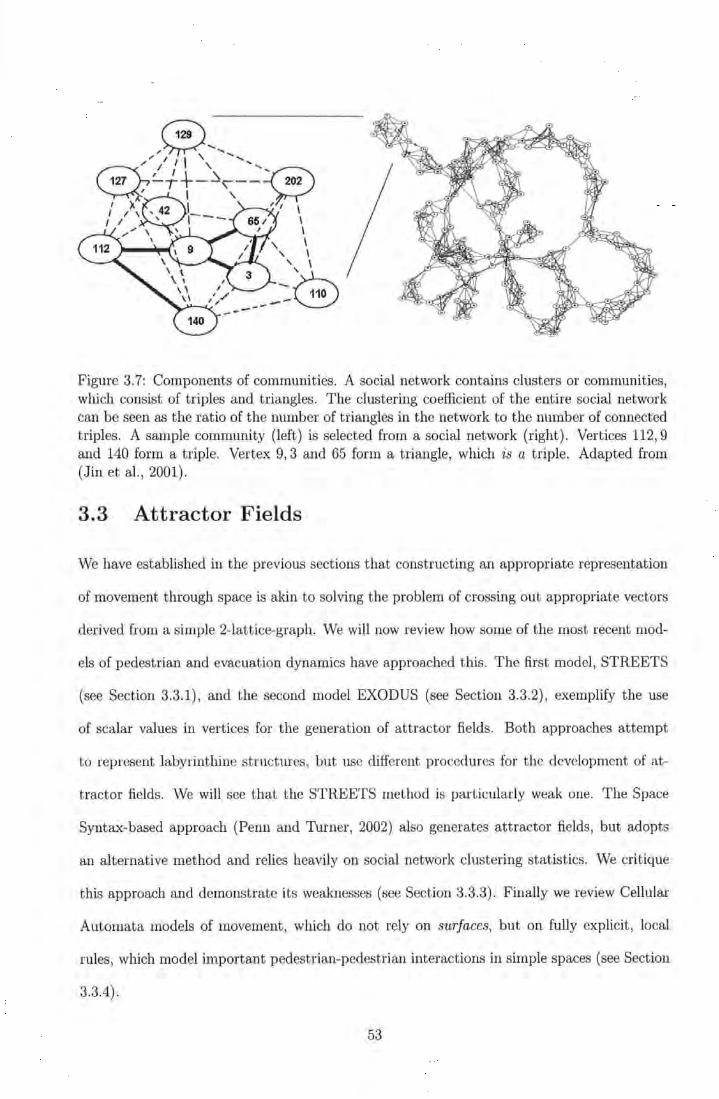
Figure 3. 7: Components of communit ies. A social network contains clusters or communities, which consist of t riples and triangles. The clustering coefficient of the ent ire social network can be seen as the ratio of the number of triangles in the network to the number of connected triples. A sample community (left) is selected from a social network (right). Vertices 112, 9 and 140 form a triple. Vertex 9, 3 and 65 form a triangle, which is a t riple. Adapted from (Jin et al. , 2001).

3.3 Attractor Fields

We have established in the previous sections that constructing an appropriate representation

of movement through space is akin to solving the problem of crossing out appropriate vectors

derived from a simple 2-lattice-graph. We will now review how some of the most recent mod-

els of pedestrian and evacuation dynamics have approached this. The first model, STREETS

(see Section 3.3.1), and the second model EXODUS (see Section 3.3.2), exemplify the use

of scalar values in vertices for the generation of attractor fields. Both approaches attempt

to represent labyrinthine structures, but use different procedures for the development of at-

tractor fields. We will see that the STREETS method is particularly weak one. The Space

Syntax-based approach (Penn and Thrner, 2002) also generates at tractor fields, but adopts

an alternative method and relies heavily on social network clustering statistics. We critique

this approach and demonstrate its weaknesses (see Section 3.3.3). Finally we review Cellular

Automata models of movement, which do not rely on surfaces, but on fully explicit, local

rules, which model important pedestrian-pedestrian interactions in simple spaces (see Section

3.3.4) .

53

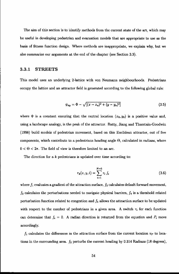
The aim of this section is to identify methods from the current state of the art, which may

be useful in developing pedestrian and evacuation models that are appropriate to use as the

basis of fitness function design. Where methods are inappropriate, we explain why, but we

also summarize our arguments at the end of the chapter (see Section 3.3).

3.3.1 STREETS

This model uses an underlying 2-lattice with von Neumann neighbourhoods. Pedestrians

occupy the lattice and an attractor field is generated according to the following global rule:

1/J:z:y =cl>- y'[(x- Xo)2 + (y- Yo)2] (3.5)

where cl> is a constant ensuring that the central location (x0 , y0 ) is a positive value and,

using a landscape analogy, is the peak of the attractor. Batty, Jiang and Thurstain-Goodwin

(1998) build models of pedestrian movement, based on this Euclidean attractor, out of five

components, which contribute to a pedestrians heading angle 8, calculated in radians, where

0 < 8 < 27T. The field of view is therefore limited to an arc.

The direction for a k pedestrians is updated over time according to:

N=5

rk(x, y,l.) = LT;/; (3.6) i=l

where fi evaluates a gradient of the attraction surface, h calculates default forward movement,

h calculates the perturbations needed to navigate physical barriers, f 4 is a threshold related

perturbation function related to congestion and / 5 allows the attraction surface to be updated

with respect to the number of pedestrians in a given area. A switch T; for each function

can determine that J; = 0. A radian direction is returned from the equation and P; move

accordingly.

/ 1 calculates the differences in the attraction surface from the current location Vp to loca-

tions in the surrounding area. h perturbs the current heading by 0.314 Radians (18 degrees),

54

Figure 3.8: A shopping mall model in STREETS. Left: mall configuration. Centre: attraction surface. Right: pedestrian positions after 100 steps. Pedestrian behaviour is determined by a surface of attraction, which is defined globally and without regard for obstacles in the space. Adapted from Batty et al. (1998).

adding a small quantity of noise to the default gradient-based movement. fa searches local eo-

ordinates for barriers E B(x, y). If the coordinates returned from !I [x±l (t+ 1), Y±l(t+ 1)] E B,

pedestrians cannot occupy them, and the !I switch is zeroed. A progress variable for each

pedestrian determines if the obstacle can be circumnavigated. These variables are incremented

each time the pedestrians encounter a new obstacle. In the event that no progress is made the

direction is reset to a random direction. The last two functions (!4 , f 5 ) relate to the interac-

tions between pedestrians. f4 provides information regarding congestion in a specified area of

space. A threshold is set in the model where 8 is again perturbed randomly if this threshold

is reached.

In an application to an idealised shopping mall, Batty et al. (1998) use equation 3.5 to define

an attraction surface. The pedestrians are then initialised to a surface, which is also populated

with obstacles. Pedestrians are attracted and converge on the middle of the shopping mall,

avoiding obstacles on the way (see Figure 3.8).

Methods in STREETS clear blockages by brute force, rather t han allowing the emergence

of naturally occurring blockage avoidance. This approach is diametrically opposed to other

pedestrian models, where blockages beget blockage or become frozen by heating (Helbing

et al., 2002). We believe this latter approach to be a much more natural representation of

real behaviour where, when blockages occur, they are reinforced; an observation made in real

55

pedestrian crowds (Canter, 1980). We believe that the reason such techniques are employed is

because the attractor field is a fixed and globally defined technique, which does not naturally

represent obstacles in the space. Any navigation is merely coded by accumulations of random

jumps. In more complex configurations than this, where empty Euclidean attraction surfaces

map poorly to labyrinthine structures, behaviour might depend largely on random walks. This

default behaviour is inefficient and, more importantly, unrealistic.

In an attempt to overcome the problems, Batty et al. (2002) introduce a stigmergy-based

approach where complex attraction surfaces are developed via incremental feedback. Each

pedestrian is located in a space representing the street layout at Notting Hill, London. The

aim for each pedestrian is to find a destination area. At the beginning of the simulation this

is done by pure random walking. However, if a pedestrian is initialised close to a destination,

then it is more likely to find it. Once a destination is found, the pedestrian moves back

to its origin, dropping pheromone on the return journey so that feedback takes hold in the

population. The attraction surface of a more complex configuration is built in this way.

However, although this approach may better represent a labyrinth, the effectiveness of the

surface will be inversely related to the number of agents used. For example, if we choose a

single agent for a complex scenario the success of the agent will depend on its initial random

position in the space. The more agents we add, the more likely each is to find the destination

through pheromone feedback.

Apart from the general criticism already made, are three specific reasons why STREETS is

of little use to us:

1. We need a method that allows agents to move over spaces of arbitrary complexity. In

this context, the methods used by Batty et al. (2002) are brittle-they require a priori

knowledge of how many pedestrians would be needed in order to generate surfaces devoid

of local minima; highly complex spaces will need many pedestrians. In an evolutionary

scenario, this knowledge will not be available because spaces will be genetically coded.

2. We cannot tolerate the default randomness in this model. The rules of behaviour seem

56

very much designed around a random-jump algorithm, to the extent that other dynamics

appear arbitrary from a modelling point of view.

3. In relation to point 2, the model does not contain any adaptive mechanism at the level

of individual pedestrians. Pedestrians follow stigmergy-based increments, accumulated

from the entire population. There is no attempt to model local processes in the context

of, individual pedestrians, situated in local conditions.

For these reasons, we abandon this approach and go on to review EXODUS. We will see

that this latter system contains methods, which are far less arbitrary, and potentially useful

for developing realistic behaviours.

3.3.2 EXODUS

The attraction surface uses the path length or depth (see above), from an origin V0 to a

destination Vd (e.g., see Figure 3.9) and obstacles are excluded form the attractor field.

Therefore, spatial navigation does not depend on random jumping behaviour for obstacle

avoidance. This is an important advantage over the methods used within STREETS. From

an evolutionary perspective it is important that randomness in a model is minimised and

certainly not a dominant feature of the dynamics.

A more general disadvantage is that EXODUS works on very detailed evacuation scenarios5.

For example, complex representations, like chemical concentrations due to fire and smoke, are

advocated (Gwynne et al., 1998) and pedestrian movement depends very much on a number

of hand-coded elements. For these reasons, EXODUS does not seem to capture the general

behaviours required of our fitness functions, which will be used to evaluate populations of

arbitrarily complex spaces. In short, the EXODUS system takes a hands-on, engineering ap

proach, which is important for specific applications, but on the basis of their lack of generality,

we exclude the use of its behavioral rules. 50f course, in some application domains, this is a strength

57

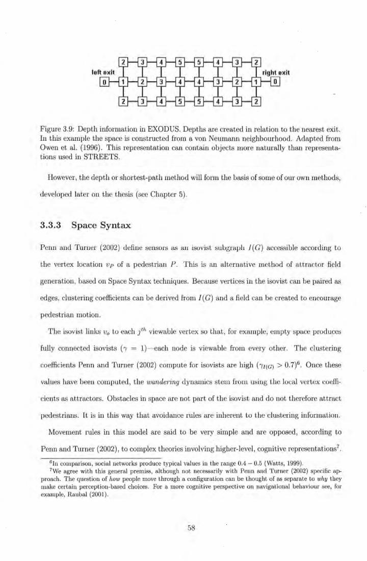
Figure 3.9: Depth information in EXODUS. Depths are created in relation to the nearest exit. In this example the space is constructed from a von Neurnann neighbourhood. Adapted from Owen et al. (1996). This representation can contain objects more naturally than representat ions used in STREETS.

However, the depth or shortest-path method will form the basis of some of our own methods,

developed later on the thesis (see Chapter 5).

3.3.3 Space Syntax

Penn and Turner (2002) define sensors as an isovist subgraph 1 (G) accessible according to

the vertex location vp of a pedestrian P. This is an alternative method of attractor field

generation, based on Space Syntax techniques. Because vertices in the isovist can be paired as

edges, clustering coefficients can be derived from I (G) and a field can be created to encourage

pedestrian motion.

The isovist links V0 to each lh viewable vertex so that, for example, empty space produces

fully connected isovists ('y = 1)-each node is viewable from every other. The clustering

coefficients Penn and Turner (2002) compute for isovists are high (t1(a) > 0.7)6 . Once these

values have been computed, the wandering dynamics stem from using the local vertex coeffi-

cients as attractors. Obstacles in space are not part of t he isovist and do not therefore attract

pedestrians. It is in this way that avoidance rules are inherent to the clustering information.

Movement rules in this model are said to be very simple and are opposed, according to

Penn and Thrner (2002), to complex theories involving higher-level, cognitive representations7.

6In comparison, social networks produce typical values in the range 0.4 - 0.5 (Watts, 1999). 7We agree with this general premiss, although not necessarily with Penn and '1\Jrner (2002) specific ap

proach. The question of how people move through a configuration can be thought of as separate to why they make certain perception-based choices. For a more cognitive perspective on navigational behaviour see, for example, Raubal (2001).

58

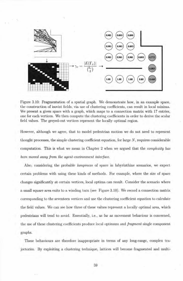
8 8 8 8 8 8

! 8 8 8 8 8 IE(f v) l

---t 'Yv = ____. 8 (;~ )

8 8888

• • •••• • • ••• -. - ··=·· . ·=·== ·. ·:::---~ii

········-· . 11111 ~~ -. ••••••••••• •

Figure 3.10: Fragmentation of a spatial graph. We demonstrate how, in an example space, the construction of isovist fields, via use of clustering coefficients, can result in local minima. We present a given space with a graph, which maps to a connection matrix with 17 entries, one for each vertices. We then compute the clustering coefficients in order to derive the scalar field values. The greyed-out vertices represent the locally optimal region.

However, although we agree, that to model pedestrian motion we do not need to represent

thought processes, the simple clustering coefficient equation, for large N, requires considerable

computation. This is what we mean in Chapter 2 when we argued that the complexity has

been moved away from the agent-environment interface.

Also, considering the probable lumpiness of space in labyrinthine scenarios, we expect

certain problems with using these kinds of methods. For example, where the size of space

changes significantly at certain vertices, local optima can result. Consider the scenario where

a small square area exits to a winding turn (see Figure 3.10). We record a connection matrix

corresponding to t he seventeen vertices and use the clustering coefficient equation to calculate

the field values. We can see how three of these values represent a locally optimal area, which

pedestrians will tend to avoid. Essentially, i.e. , as far as movement behaviour is concerned,

the use of these clustering coefficients produce local optimum and fragment single component

graphs.

These behaviours are therefore inappropriate in terms of any long-range, complex tra-

jectories. By exploit ing a clustering technique, lattices will become fragmented and multi-

59

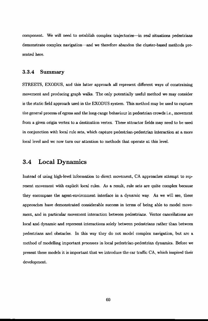
component. We will need to establish complex trajectories-in real situations pedestrians

demonstrate complex navigation-and we therefore abandon the cluster-based methods pre

sented here.

3.3.4 Summary

STREETS, EXODUS, and this latter approach all represent different ways of constraining

movement and producing graph walks. The only potentially useful method we may consider

is the static field approach used in the EXODUS system. This method may be used to capture

the general process of egress and the long-range behaviour in pedestrian crowds i.e., movement

from a given origin vertex to a destination vertex. These attractor fields may need to be used

in conjunction with local rule sets, which capture pedestrian-pedestrian interaction at a more

local level and we now turn our attention to methods that operate at this level.

3.4 Local Dynamics

Instead of using high-level information to direct movement, CA approaches attempt to rep

resent movement with explicit local rules. As a result, rule sets are quite complex because

they encompass the agent-environment interface in a dynamic way. As we will see, these

approaches have demonstrated considerable success in terms of being able to model move

ment, and in particular movement interaction between pedestrians. Vector cancellations are

local and dynamic and represent interactions solely between pedestrians rather than between

pedestrians and obstacles. In this way they do not model complex navigation, but are a

method of modelling important processes in local pedestrian-pedestrian dynamics. Before we

present these models it is important that we introduce the car traffic CA, which inspired their

development.

60

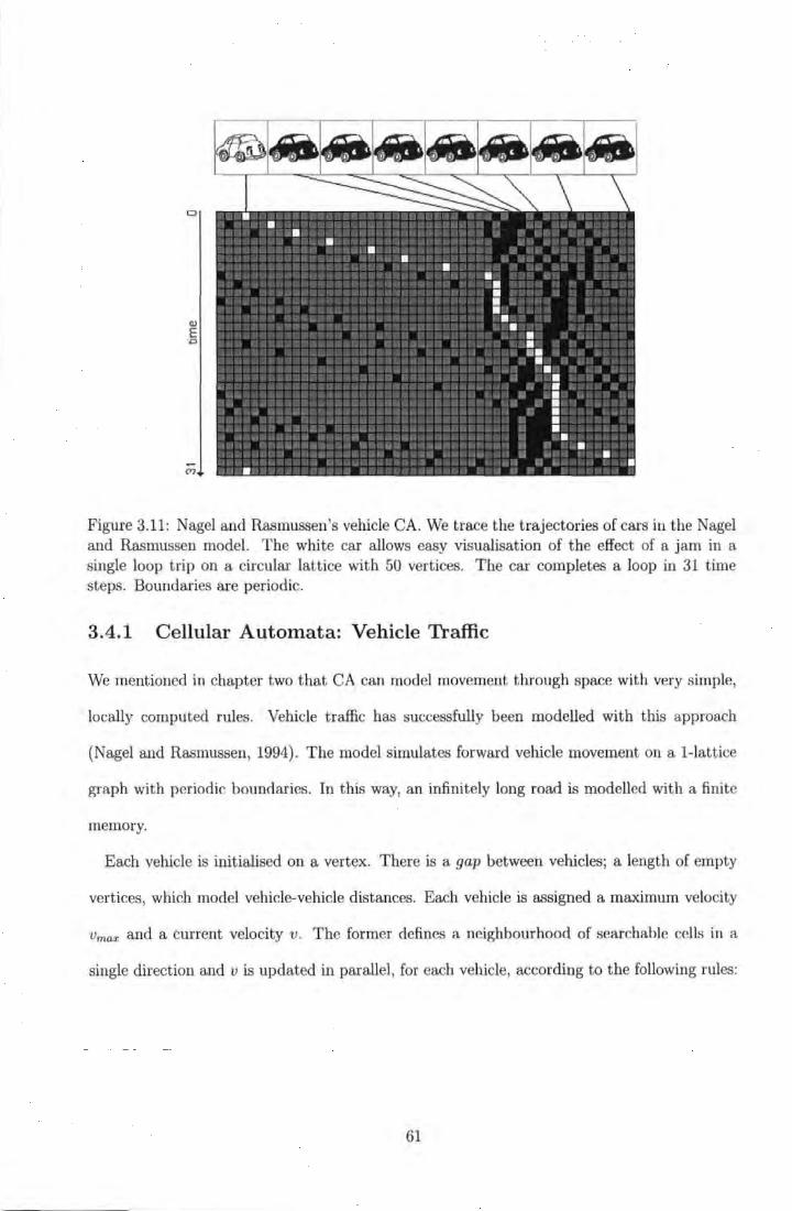
Figure 3.11: Nagel and Rasmussen's vehicle CA. We trace the trajectories of cars in the Nagel and Rasmussen model. The white car allows easy visualisation of the effect of a jam in a single loop trip on a circular lattice with 50 vertices. The car completes a loop in 31 time steps. Boundaries are periodic.

3.4.1 Cellular Automata: Vehicle Traffic

We mentioned in chapter two that CA can model movement through space with very simple,

locally computed rules. Vehicle traffic has successfully been modelled with this approach

(Nagel and Rasmussen, 1994) . The model simulates forward vehicle movement on a !-lat t ice

graph with periodic boundaries. In this way, an infinitely long road is modelled with a finite

memory.

Each vehicle is initialised on a vertex. There is a gap between vehicles; a length of empty

vertices, which model vehicle-vehicle distances. Each vehicle is assigned a maximum velocity

Vmax and a current velocity v . The former defines a neighbourhood of searchable cells in a

single direction and v is updated in parallel, for each vehicle, according to the following rules:

61

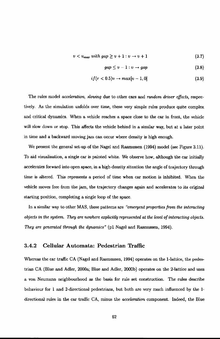
V < Vma.x with gap 2: V + 1 : V --+ V + 1

gap :::; v - 1 : v --+ gap

if(r < 0.5)v --+ max[v- 1, 0]

(3.7)

(3.8)

(3.9)

The rules model acceleration, slowing due to other cars and random driver effects, respec

tively. As the simulation unfolds over time, these very simple rules produce quite complex

and critical dynamics. When a vehicle reaches a space close to the car in front, the vehicle

will slow down or stop. This affects the vehicle behind in a similar way, but at a later point

in time and a backward moving jam can occur where density is high enough.

We present the general set-up of the Nagel and Rasmussen (1994) model (see Figure 3.11).

To aid visualisation, a single car is painted white. We observe how, although the car initially

accelerates forward into open space, in a high-density situation the angle of trajectory through

time is altered. This represents a period of time when car motion is inhibited. When the

vehicle moves free from the jam, the trajectory changes again and accelerates to its original

starting position, completing a single loop of the space.

In a similar way to other MAS, these patterns are "emergent properties from the interacting

objects in the system. They are nowhere explicitly represented at the level of interacting objects.

They are generated through the dynamics" (pl Nagel and Rasmussen, 1994).

3.4.2 Cellular Automata: Pedestrian Thaffic

Whereas the car traffic CA (Nagel and Rasmussen, 1994) operates on the 1-lattice, the pedes

trian CA (Blue and Adler, 2000a; Blue and Adler, 2000b) operates on the 2-la.ttice and uses

a von Neumann neighbourhood as the basis for rule set construction. The rules describe

behaviour for 1 and 2-directional pedestrians, but both are very much influenced by the 1-

directional rules in the car traffic CA, minus the acceleration component. Indeed, the Blue

62

and Adler (2000a) model can be seen as an extension of the Nagel and Rasmussen (1994)

model. The latter captures interesting properties of vehicle flow in real traffic and the the aim

is that pedestrian dynamics be modelled with a similar degree of success.

One frequently observed pattern in real pedestrian systems is the formation of lanes. People

make different decisions based on which direction another person is moving. For example, in

the simplest case, two people moving in the same direction are likely to have a similar velocity

where few or no interactions take place. If two people are moving in opposite directions and

in the same lane, then there will be decisions to make regarding collision avoidance. The

rule sets of Blue and Adler (2000a) are an attempt to model these kinds of decisions, which

optimise forward movement.

Because the space is extended to two dimensions and there are contra-flows, the rule sets

are far more complex than the Nagel and Rasmussen (1994) model. We present the Blue and

Adler (2000a) rule sets (see Table 3.1).

As a self-organising model, it is difficult to fully appreciate by simply considering printed

rule sets. We implement the model and present a graphical snapshot when behaviour has

settled for both !-directional and 2-directional populations (see Figure 3.12 Top). We can see

lane formations in the 2-directional case and for !-directional movements we observe mode

locking (Blue and Adler, 2000a). In order to present the dynamics in this model, we need to

sample a 1-D lane from 2-D space and watch how it changes through time. We observe how

lanes develop towards either west or east moving pedestrians (see Figure 3.12 bottom).

3.5 Summary

At the beginning of this chapter, we provided some important definitions, and then provided

a more in-depth review of discrete dynamical methods, which we classified according to:

• Attractor Fields

Fields need to be constructed so that no local optima exist. STREETS and Space

63

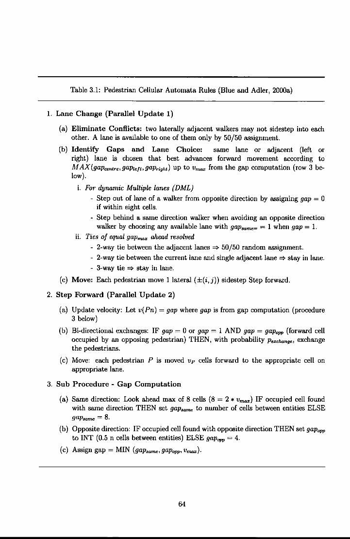
Table 3.1: Pedestrian Cellular Automata Rules (Blue and Adler, 2000a)

1. Lane Change (Parallel Update 1)

(a) Eliminate Conflicts: two laterally adjacent walkers may not sidestep into each other. A lane is available to one of them only by 50/50 assignment.

(b) Identify Gaps and Lane Choice: same lane or adjacent (left or right) lane is chosen that best advances forward movement according to M AX(gapcentre, gapleft• gapright) up to vma:J: from the gap computation (row 3 below).

i. For dynamic Multiple lanes {DML)

- Step out of lane of a walker from opposite direction by assigning gap = 0 if within eight cells.

- Step behind a same direction walker when avoiding an opposite direction walker by choosing any available lane with gapsame= = 1 when gap = 1.

u. Ties of equal gapma:z; ahead resolved

- 2-way tie between the adjacent lanes => 50/50 random assignment.

- 2-way tie between the current lane and single adjacent lane => stay in lane. - 3-way tie => stay in lane.

(c) Move: Each pedestrian move 1lateral (±(i,j)) sidestep Step forward.

2. Step Forward (Parallel Update 2)

(a) Update velocity: Let v(Pn) =gap where gap is from gap computation (procedure 3 below)

(b) Bi-directional exchanges: IF gap= 0 or gap= 1 AND gap= gapupp (forward cell occupied by an opposing pedestrian) THEN, with probability Pexchange, exchange the pedestrians.

(c) Move: each pedestrian P is moved vp cells forward to the appropriate cell on appropriate lane.

3. Sub Procedure - Gap Computation

(a) Same direction: Look ahead max of 8 cells (8 = 2 * vma:J:) IF occupied cell found with same direction THEN set gap8ame to number of cells between entities ELSE gapsame = 8.

(b) Opposite direction: IF occupied cell found with opposite direction THEN set gapupp to INT (0.5 n cells between entities) ELSE gapupp = 4.

(c) Assign gap= MIN (gap80me,gapupp,vma:z;).

64

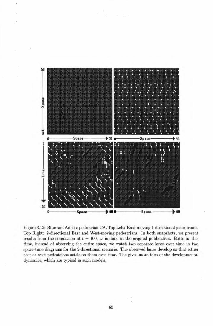
50

Ill u ~ 1:1.

I 0

0

Ill E

1 Figure 3.12: Blue and Adler's pedestrian CA. Top Left: East-moving !-directional pedestrians. Top llight: 2-directional East and West-moving pedestrians. In both snapshots, we present results from the simulation at t = 100, as is done in the original publication. Bottom: this time, instead of observing the entire space, we watch two separate lanes over time in two space-time diagrams for the 2-directional scenario. The observed lanes develop so that either east or west pedestrians settle on them over time. The gives us an idea of the developmental dynamics, which are typical in such models.

65

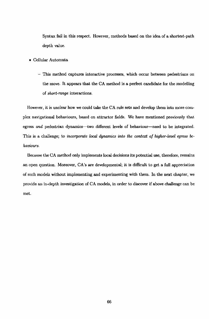
Syntax fail in this respect. However, methods based on the idea of a shortest-path

depth value.

• Cellular Automata

- This method captures interactive processes, which occur between pedestrians on

the move. It appears that the CA method is a perfect candidate for the modelling

of short-mnge interactions.

However, it is unclear how we could take the CA rule sets and develop them into more com

plex navigational behaviours, based on attractor fields. We have mentioned previously that

egress and pedestrian dynamics-two different levels of behaviour-need to be integrated.

This is a challenge; to incorpomte local dynamics into the context of higher-level egress be

haviours.

Because the CA method only implements local decisions its potential use, therefore, remains

an open question. Moreover, CA's are developmental; it is difficult to get a full appreciation

of such models without implementing and experimenting with them. In the next chapter, we

provide an in-depth investigation of CA models, in order to discover if above challenge can be

met.

66

Chapter 4

Cellular Automata

The primary aim of this chapter is to explore the usefulness of pedestrian CA models by

replicating and investigating them in further detail. We are particularly interested in their

robustness and portability. Therefore, our investigations revolve around the following ques

tions: Is behaviour robust across varying levels of density? Do behaviours at varying densities

show sensible statistical characteristics? If so, can we transport the model easily to spaces of

arbitrary complexity? If not, can we sufficiently improve the CA in order to achieve these

ends?

In the first two sections we take a close look at the statistical behaviour of the vehicle

CA (see Section 4.1), as a precursor to the pedestrian CA model (see Section 4.2), which

we interrogate quantitatively and qualitatively. Conclusions from the investigation lead to

attempts at model improvement (see Section 4.3). FUrthermore, we attempt to integrate an

improved model with attractor field methods of pedestrian movement (see Section 4.4). We

present answers to the above questions in the form of empirical results, discussion of findings.

We provide an extensive summary and discussion at the end of the chapter {see Section 4.5),

which marks a pivotal point in the thesis.

67

4.1 1-D CA: Vehicles

The rerumn we implement, test and replicate this model will become clearer later, when we

look at the 2-D pedestrian model (Blue and Adler, 2000a). Both models use a similar kind of

search to help optimise forward movement, although the pedestrian model extends this search

to 2-D scenarios. It is therefore useful to look in more detail at the Nagel and Rasmussen

(1994) model.

4.1.1 Statistical Behaviour

We have already seen how jams can form in the Nagel and Rasmussen (1994) model and how

this affects vehicle velocity (see Section 3.4.1). Nagel and Rasmussen (1994) study jams over

a range of density p. Increasing p introduces more cars into the system and is associated with

different regimes of behaviour. Nagel and Rasmussen (1994) measure the travel time of a car

as it passes through a sublattice section of the model road. This produces an array of travel

times for each car, as they moves along the 1-lattice, entering and exiting the sampled section.

The simulation runs for 105 time steps. Travel time is simply the average time spent inside

the sampled space and its variation a is defined as:

(4.1)

where ( ... ) denotes the average travel time for all cars in the simulation. This is the coeffi-

cient of variation of the array of times recorded for each vehicle.

We interpret the basic intuition of Equation 4.1 as the shape of car movement, highlighted

again by a white car, in a space-time plot (see Figure 4.1). At low density (p = 0.08) the

white line runs smoothly across the plot where perturbations to movement are small and

infrequent. At high density (p = 0.8) this line changes angle, representing slower movement.

Perturbations to this movement are again relatively small, but frequent. In the middle regime

(p = 0.16) the fluctuations are high and fairly frequent. This represents a critical regime

68

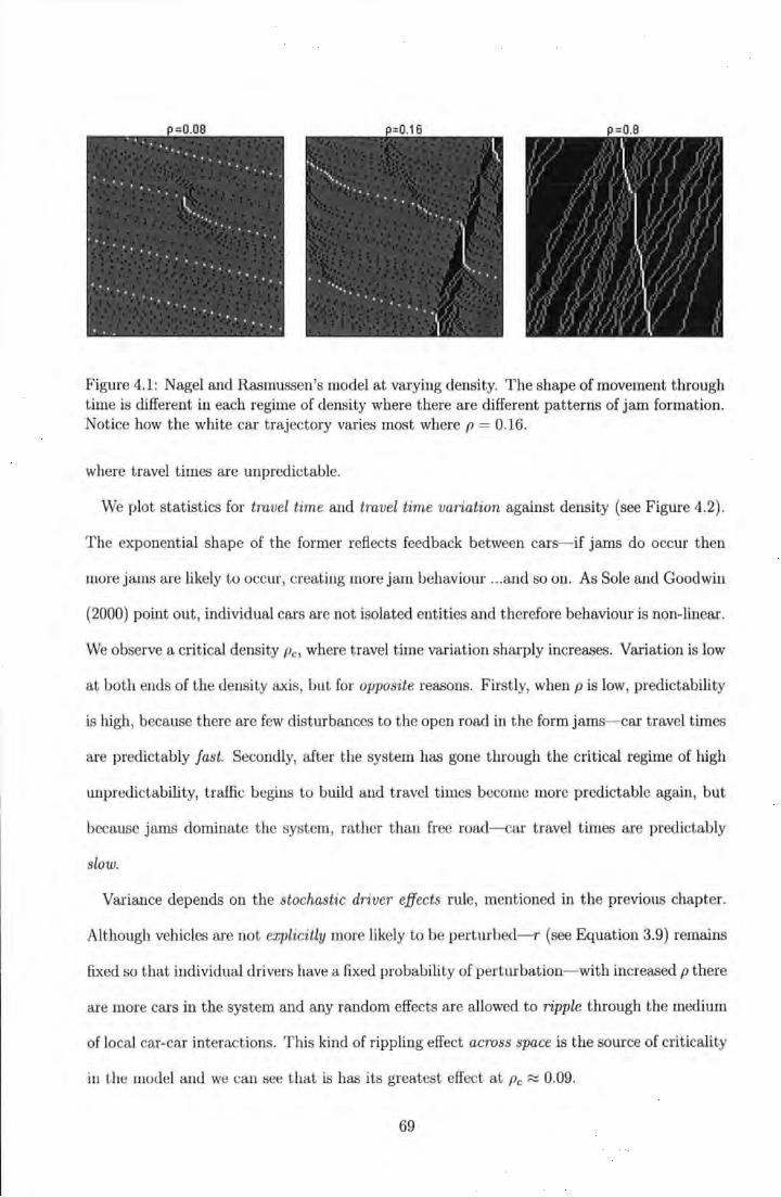
' I '

I. I.

········,· .... . . . . . . . ··, .. "l

·· ... . . ·· .... . . . . .

. . . . . ,1

Figure 4.1: Nagel and Rasmussen's model at varying density. The shape of movement through time is different in each regime of density where there are different patterns of jam formation. Notice how the white car trajectory varies most where p = 0.16.

where travel times are unpredictable.

We plot statistics for travel time and travel time variation against density (see Figure 4.2) .

The exponential shape of the former reflects feedback between cars-if jams do occur then

more jams are likely to occur, creating more jam behaviour ... and so on. As Sole and Goodwin

(2000) point out, individual cars are not isolated entities and therefore behaviour is non-linear.

We observe a critical density Pc, where travel time variation sharply increases. Variation is low

at both ends of the density axis, but for opposite reasons. Firstly, when pis low, predictability

is high, because there are few disturbances to the open road in the form jams-car travel times

are predictably fast. Secondly, after the system has gone through the critical regime of high

unpredictability, traffic begins to build and travel times become more predictable again, but

because jams dominate the system, rather than free road-car travel times are predictably

slow.

Variance depends on the stochastic driver effects rule, mentioned in the previous chapter.

Although vehicles are not explicitly more likely to be perturbed-r (see Equation 3.9) remains

fixed so that individual drivers have a fixed probability of perturbation- with increased p there

are more cars in the system and any random effects are allowed to ripple through the medium

of local car-car interactions. This kind of rippling effect across space is the source of criticality

in the model and we can see that is has its greatest effect at Pc~ 0.09.

69

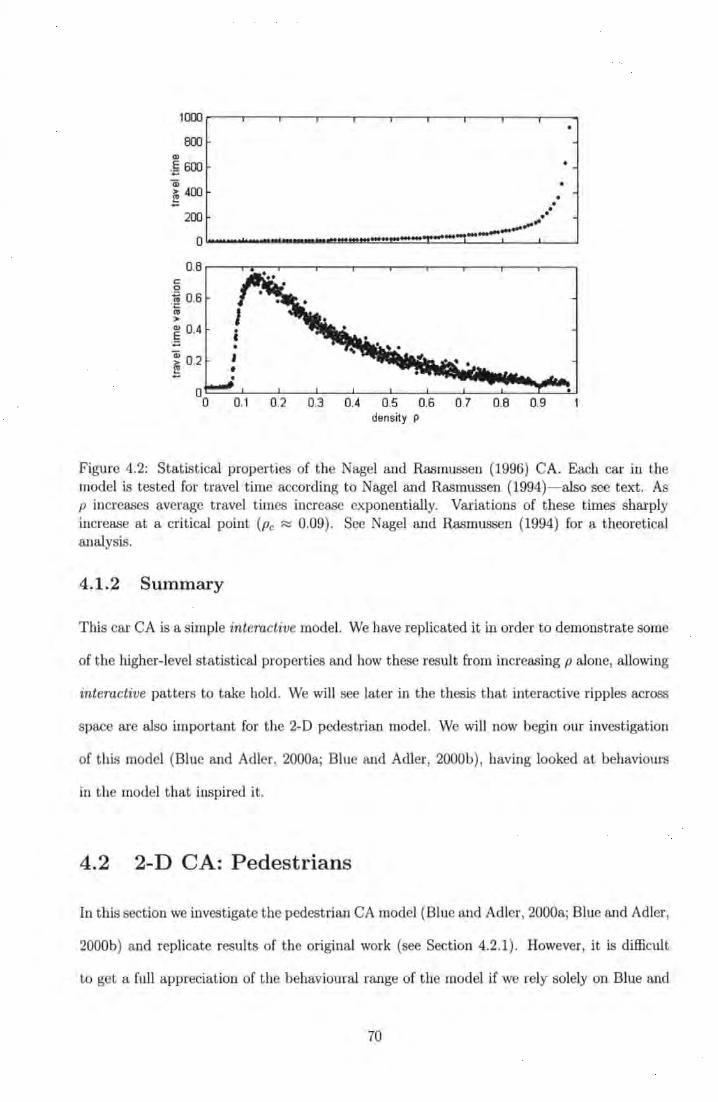
10CD~--.---.---.----.---.---.--~.---.---,---~

800 Ql

·~ 600 • m • f 400 ••

• D ~ _.,..fill"' o~--~~~~~~~-~-~-~~·-~-~·~~·-~-=·~~·------L--~--~

0.8 .-----.-.---,.---.----.----.---.----.---.---,-----, c 0

~ 0.6 ·c "' ,.. E o.4

·.;::;

' • 0.1 0.2 0.3 0.4 0.5 0.6 0.7 0.8 0.9

density P

Figure 4.2: Statistical properties of the Nagel and Rasmussen (1996) CA. Each car in the model is tested for travel time according to Nagel and Rasmussen (1994)- also see text. As p increases average travel times increase exponentially. Variations of these times sharply increase at a critical point (Pc ~ 0.09). See Nagel and Rasmussen (1994) for a theoretical ar1alysis.

4.1.2 Summary

This car CA is a simple interactive model. We have replicated it in order to demonstrate some

of the higher-level statistical properties and how these result from increasing p alone, allowing

interactive patters to take hold. We will see later in the thesis that interactive ripples a{:rOSS

space are also important for the 2-D pedestrian model. We will now begin our investigation

of this model (Blue and Adler, 2000a; Blue and Adler, 2000b) , having looked at behaviours

in the model that inspired it.

4.2 2-D CA: Pedestrians

In this section we investigate the pedestrian CA model (Blue and Adler, 2000a; Blue and Adler,

2000b) and replicate results of the original work (see Section 4.2.1) . However, it is difficult

to get a full appreciation of the behavioural range of the model if we rely solely on Blue and

70

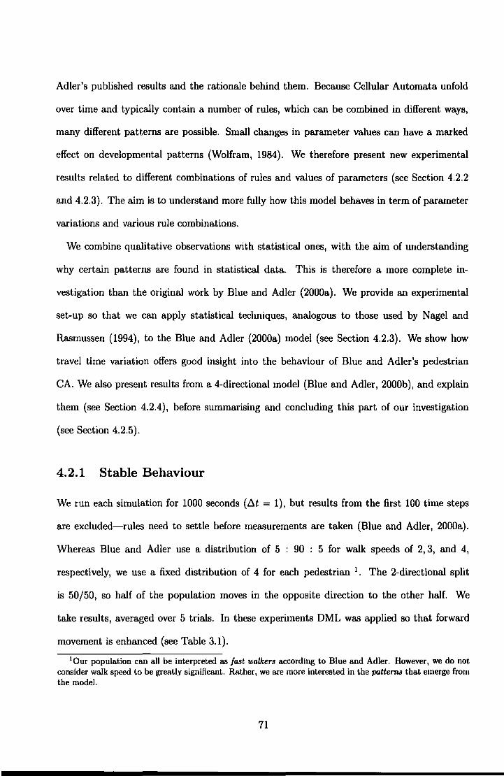
Adler's published results and the rationale behind them. Because Cellular Automata unfold

over time and typically contain a number of rules, which can be combined in different ways,

many different patterns are possible. Small changes in parameter values can have a marked

effect on developmental patterns (Wolfram, 1984). We therefore present new experimental

results related to different combinations of rules and values of parameters (see Section 4.2.2

and 4.2.3). The aim is to understand more fully how this model behaves in term of parameter

variations and various rule combinations.

We combine qualitative observations with statistical ones, with the aim of understanding

why certain patterns are found in statistical data. This is therefore a more complete in-

vestigation than the original work by Blue and Adler (2000a). We provide an experimental

set-up so that we can apply statistical teclmiques, analogous to those used by Nagel and

Rasmussen (1994), to the Blue and Adler (2000a) model (see Section 4.2.3). We show how

travel time variation offers good insight into the behaviour of Blue and Adler's pedestrian

CA. We also present results from a 4-directional model (Blue and Adler, 2000b), and explain

them (see Section 4.2.4), before summarising and concluding this part of our investigation

(see Section 4.2.5).

4.2.1 Stable Behaviour

We run each simulation for 1000 seconds (lH = 1), but results from the first 100 time steps

are excluded-rules need to settle before measurements are taken (Blue and Adler, 2000a).

Whereas Blue and Adler use a distribution of 5 : 90 : 5 for walk speeds of 2, 3, and 4,

respectively, we use a fixed distribution of 4 for each pedestrian 1 • The 2-directional split

is 50/50, so half of the population moves in the opposite direction to the other half. We

take results, averaged over 5 trials. In these experiments DML was applied so that forward

movement is enhanced (see Table 3.1).

10ur population can all be interpreted IlB fast walkers according to Blue and Adler. However, we do not consider walk speed to be greatly significant. Rather, we are more interested in the patterns that emerge from the model.

71

100 -+-- directional

!ll -- bi-directional

00

70

60

"C

"' 50 CV a.

"' 40

:JJ

20

10

00 0.1 0.2 0.3 0.4 0.5 0.6 0.7 O.B 0.9 density

Figure 4.3: Directional and 2-directional speed-density statistics. 2-directional behaviour is less optimal where p > 0.1. However, the shape of t he curves begin to differ where p = 0.2. Speed = 4V Pi .

We observe population average speed for 1 and 2-directional scenarios (see Figure 4.3).

Results confirm observations made by Blue and Adler (2000a) where !-directional populations

optimise forward movement more effectively than 2-directional ones. We observe a large

decrease in total speed in t he 2-directional population compared to the 1-directional population

(p = 0.2- 0.3). This suggests that the rules function more effectively at different densities-

lane formations appear particularly robust at lower densities (p =< 0.3) . At higher density

(p => 0.3) performance is poorer. However, because speed decays relatively slowly after this

density, the lane-formation rules appear to succeed to some extent across the entire density

range.

We might conclude that lane formations are robust because forward movement is maintained

over this broad range. Only in a special case (p = 1) do we observe zero movement. With these

results it is tempting to assume that the lane formation rules will still be at work in situations

of high density, particularly when we consider the local intuition of the rule sets. Further, we

may be forgiven for thinking that smooth decay indicates a relatively slow deterioration of

lane formation patterns.

72

In order to test these assumptions and uncover the true robustness of lane-formation rule-

sets, we now investigate the effects of what we believe to be important parameters in the

model, particularly with respect to these higher-level patterns of lane-formation. If there are

any shortcomings in the model we need to reveal and understand them and the investigations

of the following sections are designed with this in mind.

4.2.2 Testing Robustness

Blue and Adler (2000a) only present graphical snapshot diagrams of the kind seen in chapter

2 where mode-locking in 1-directional scenarios, or lane-formation in 2-directional scenarios

occurs (p ~ 0.2). We run the model at higher densities (p = 0.4) where statistical results

(see Figure 4.3) indicate the population to have reached a relatively poor performance level.

In order to allow the model to fully escape from the randomness of initialisation, we take

snapshots at t = 200 and record results for three different values of PexcluJnge·

The reason we do this is because we believe that P uchange is an important source of variation

in the model and also an important factor in the formation (or lack of formation) of lanes.

Essentially, this is because the P exchange parameter provides the condition on which pedestrians

with opposing directions make an exchange and remain in the same lane. This works against

the rest of the rules, which allow development away from random initialisation and towards

bi-directional lane splits. We present results (see Figure 4.4) and make the following three

observations:

1. We observe that the smooth decay of the speed-density statistics (above) do not result

from the gradual disappearance of 2-directionallane formations. Most of the population

are in a state of conflict, where clusters have formed and dominate the entire lattice

(see Figure 4.4, Left) 2 .

2 An interesting dynamical property of these clusters is that they tend to persist by moving around the lattice, sucking in and spitting out different pedestrians. In this way the clusters are persistent entities in themselves, which emerge from the model, but as unintended side effects.

73

. .

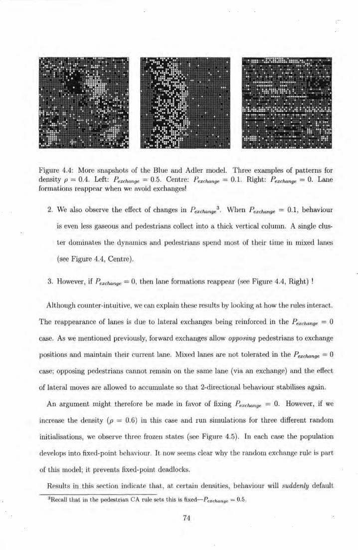
. . . .. .. .. .. I I I ••':'' I ~~=

. . . .. .. .

.... .... . . . . . .. . . . . . . . . ....... 11 I I ......... ....... . ............. ..... ... . . . ...... . ........

. . .

· ·· ::i:s:::: .. . .. : :u :;: :.: .:: .• : . ... . . . . . . ..

11 I I . . . . . ...... . I I 11 . . . ... . .. . . . . . ... . . .. : . . . . .. .. .. . .... .. .... .. .

. . . .. . . ....... ... ...... ..... I 11111 I .. · .. ·.:· . .... . . .

I I I I I 11 . . . I Ill .... ...... ........ . . .. ... .... . . .... . .. .

11 I 11 I

. .. . .. . . . . :: :

I Ill I I I ... . . .. .... . . ··.· :.·::: . . .... .. ·::.: I I I I I I 111111 .............

11 11: 11:111111 I

• :::=·:=:.::: : •• .. .... . .. . ::::.;::=!!~;; . . ·.· .·:.:::· .. . ... .. . .. . .. .. ... . .. . . ... :.·.:.·:: ::·.:. ... . ..... . ·.:·· : :·.···.:· ....... :·: .. · 11 11 Ill I I I ... . ..... . ... ··::. .. :::. . . . ...... . . • .... · .. ·:::.: : .. . .. . ..... . ·.·: ·:::·.· .. . .. . ..... . .. ··.·.:::· .. : ... . . .. . .... . ... .... ... . . . .. . .. .. .. . . .. .. . . ... . ..

. .

Figure 4.4: More snapshots of the Blue and Adler model. Three examples of patterns for density p = 0.4. Left: P exchange = 0.5. Centre: P exchange = 0.1. Right: P exchange = 0. Lane formations reappear when we avoid exchanges!

2. We also observe the effect of changes in P exchange 3 . When P exchange = 0.1, behaviour

is even less gaseous and pedestrians collect into a thick vertical column. A single clus-

ter dominates the dynamics and pedestrians spend most of their time in mixed lanes

(see Figure 4.4, Centre) .

3. However, if ?exchange= 0, then lane formations reappear (see Figure 4.4, Right) !

Although counter-intuitive, we can explain these results by looking at how the rules interact.

The reappearance of lanes is due to lateral exchanges being reinforced in the ? exchange = 0

case. As we mentioned previously, forward exchanges allow opposing pedestrians to exchange

positions and maintain their current lane. Mixed lanes are not tolerated in the P exchange = 0

case; opposing pedestrians cannot remain on the same lane (via an exchange) and the effect

of lateral moves are allowed to accumulate so that 2-directional behaviour stabilises again.

An argument might therefore be made in favor of fixing P exchange = 0. However, if we

increase the density (p = 0.6) in this case and run simulations for three different random

initialisations, we observe three frozen states (see Figure 4.5). In each case the population

develops into fixed-point behaviour. It now seems clear why the random exchange rule is part

of this model; it prevents fixed-point deadlocks.

Results in this section indicate that, at certain densities, behaviour will suddenly default

3 Recall that in the pedestrian CA rule sets this is fixed- P exchangc = 0.5.

74

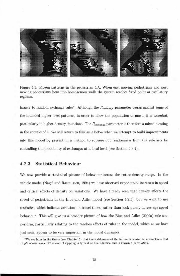
Figure 4.5: Frozen patterns in the pedestrian CA. When east moving pedestrians and west moving pedestrians form into homogenous walls the system reaches fixed point or oscillatory regimes.

largely to random exchange rules4 . Although the ? exchange parameter works against some of

the intended higher-level patterns, in order to allow the population to move, it is essential,

particularly in higher-density situations. The ? exchange parameter is therefore a mixed blessing

in the context of p. We will return to this issue below when we attempt to build improvements

into this model by presenting a method to squeeze out randomness from the rule sets by

controlling the probability of exchanges at a local level (see Section 4.3.1).

4.2.3 Statistical Behaviour

We now provide a statistical picture of behaviour across the entire density range. In the

vehicle model (Nagel and R.asmussen, 1994) we have observed exponential increases in speed

and critical effects of density on variations. We have already seen that density affects the

speed of pedestrians in the Blue and Adler model (see Section 4.2.1) , but we want to use

statistics, which indicate variations in travel times, rather than look purely at average speed

behaviour. This will give us a broader picture of how the Blue and Adler (2000a) rule sets

perform, particularly relating to the random effects of rules in the model, which as we have

just seen, appear to be very important in the model dynamics.

4 We see later in the thesis (see Chapter 5) that the suddenness of the failure is related to interactions that ripple across space. This kind of rippling is typical on the 2-lattice and is known a percolation.

75

Because the vehicle model is 1-D and the pedestrian model is 2-D, the experimental set

up used by Nagel and Rasmussen (1994) is not directly applicable. We therefore use the

following experimental set-up for the Blue and Adler model in order to apply similar statistical

techniques.

Experimental set-up: We allocate to each pedestrian Pt a value a;, which defines a

desired number of steps to be made in a given direction. Three separate populations of

pedestrians P1, pm and pn are defined where Vmaz is set to 1, 2, and 4, respectively and

a= 100 VP•. With flt = 1, we record t VP•, when the halting condition (a;= 100) is met

and apply this scenario for a range of densities p = (0, 0.8). Three separate simulations are

used for each population. We make four observations:

1. As we would expect, travel times in each population exponentially increase (see Figure

4.6, Top), for similar reasons to results obtained from the Nagel and Rasmussen (1994)

model.

2. However, in contrast to the Nagel and Rasmussen (1994) model, the travel time varia

tions continue to rise (see Figure 4.6, Bottom). This occurs because, with increases to

density p, random exchanges increase and the variations in travel times reflect increased

randomness all the way through the density range.

3. Populations P1, pm and pn with different values for Vmaz have different travel-time

variation patterns as a function of density. The parameter Vma.x determines the potential

amount of space available for search. Therefore, at low densities, for pn (vmaz = 4),

neighbourhood search is more likely to be affected by oncoming pedestrians compared

with pm (vmax = 2). We also expect pm to be more likely affected than P(vmaz = 1)

for the same reason.

4. Convergence of variations at p = 0.58. Above p = 0.5, the majority of space is occupied

and randomness influences movement regardless of the Vmaz value because each popula-

76

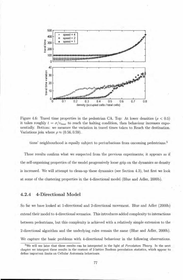
~r----.----.-----~--~r---~----~----~--~

400 " speed= 4 + speed= 2 + speed= 1

100=======-...-111"'"' o~--~----~----~--~L---~----~----~--~

40.----.----.-----.-----r----.----.-----.----. c 0

·~ 30 ·~ > "'20

.~ -a; 10 ~

0.6 0.7 0.8 density (occupied cells /total cells)

Figure 4.6: 'fravel time properties in the pedestrian CA. Top: At lower densities (p < 0.5) it takes roughly t = CI fvmax to reach the halting condition, then behaviour increases exponentially. Bottom: we measure the variation in travel times taken to Reach the destination. Variations join where p ~ (0.56, 0.59).

tions' neighbourhood is equally subject to perturbations from oncoming pedestrians.5

These results confirm what we suspected from the previous experiments; it appears as if

the self-organising properties of the model progressively loose grip on the dynamics as density

is increased. We will attempt to clean-up these dynamics (see Section 4.3), but first we look

at some of the clustering properties in the 4-directional model (Blue and Adler, 2000b).

4.2.4 4-Directional Model

So far we have looked at !-directional and 2-directional movement. Blue and Adler (2000b)

extend their model to 4-directional scenarios. This introduces added complexity to interactions

between pedestrians, but this complexity is achieved with a relatively simple extension to the

2-directional algorithm and the underlying rules remain the same (Blue and Adler, 2000b).

We capture the basic problems with 4-directional behaviour in the following observations.

5 We will see later that these results can be interpreted in the light of Percolation Theory. ln the next chapter we interpret these results in the context of 2-lattice Boolean percolation statistics, which appear to define important limits on Cellular Automata behaviours.

77

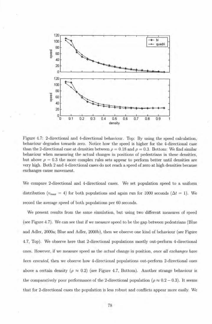
120

100

80 -o Q)

60 Q)

0.. (/)

40

20

0

120

100

80 -o Q)

60 Q) 0.. (/)

40

20

0 0 0.1 0.2 0.3 0.4 0.5 0.6 0.7 0.8 0.9

density

Figure 4.7: 2-directional and 4-directional behaviour. Top: By using the speed calculation, behaviour degrades towards zero. Notice how the speed is higher for the 4-directional case than the 2-directional case at densities between p = 0.18 and p = 0.3. Bottom: We find similar behaviom when measming the actual changes in positions of pedestrians in these densities, but above p = 0.3 the more complex rules sets appear to perform better until densities are very high. Both 2 and 4-directional cases do not reach a speed of zero at high densities because exchanges cause movement.

We compare 2-directional and 4-directional cases. We set population speed to a uniform

distribution (vmax = 4) for both populations ar1d again run for 1000 seconds (tl t = 1). We

record the average speed of both populations per 60 seconds.

We present results from the same simulation, but using two different measures of speed

(see Figure 4.7). We can see that if we measure speed to be the gap between pedestrians (Blue

and Adler, 2000a; Blue and Adler, 2000b), then we observe one kind of behaviour (see Figure

4.7, Top) . We observe here that 2-directional populations mostly out-perform 4-directional

ones. However, if we measure speed as the actual change in posit ion, once all exchanges have

been executed, then we observe how 4-directional populations out-perform 2-directional ones

above a certain density (p ~ 0.2) (see Figure 4.7, Bottom). Another strange behaviour is

the comparatively poor performance of the 2-directional population (p ~ 0.2- 0.3) . It seems

that for 2-directional cases the population is less robust and conflicts appear more easily. We

78

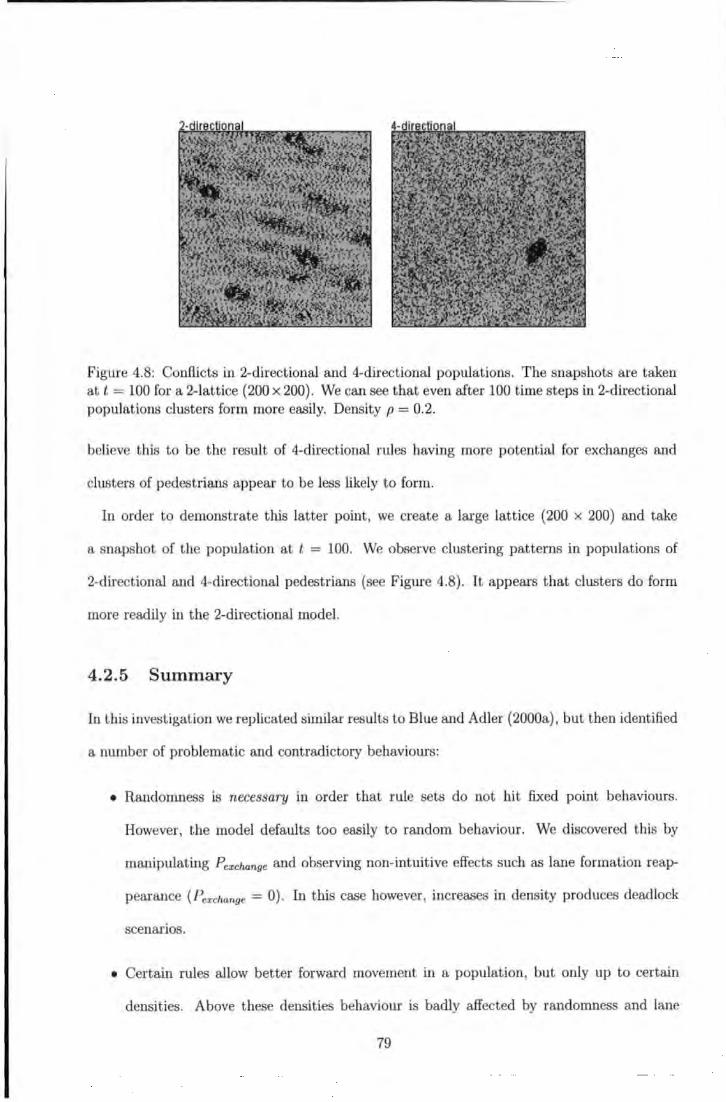
Figure 4.8: Conflicts in 2-directional and 4-directional populations. The snapshots are taken at t = 100 for a 2-lattice (200 x 200) . We can see that even after 100 time steps in 2-directional populations clusters form more easily. Density p = 0.2.

believe this to be the result of 4-directional rules having more potential for exchanges and

clusters of pedestrians appear to be less likely to form.

In order to demonstrate this latter point, we create a large lattice (200 x 200) and take

a snapshot of the population at t = 100. We observe clustering patterns in populations of

2-directional and 4-directional pedestrians (see Figure 4.8). It appears that clusters do form

more readily in the 2-directional model.

4.2.5 Summary

In this investigation we replicated similar results to Blue and Adler (2000a), but then identified

a number of problematic and contradictory behaviours:

• Randomness is necessary in order that rule sets do not hit fixed point behaviours.

However, the model defaults too easily to random behaviour. We discovered this by

manipulating P ezchange and observing non-intuitive effects such as lane formation reap-

pearance (Pezchange = 0) . In this case however, increases in density produces deadlock

scenarios.

• Certain rules allow better forward movement in a population, but only up to certain

densities. Above these densities behaviour is badly affected by randomness and lane

79

formation patterns disappear. In contrast to what we might expect with this model

that the effect of self-organising rules gradually deteriorate-we observe that breakdown

occurs fairly suddenly.

• We further tested the robustness of the 2-directional model with a simple experiment,

which provided a statistical picture of the effect density on populations with a different

search capacity, defined by the parameter Vmax· However, at certain densities, there is

only one picture; runaway random behaviour.

• We have demonstrated how anomalies are inherent in 4-directional populations, which

perform equally well or sometimes better than 2-directional populations, depending on

parameter values. We argued that this is also due to inherent randomness of the rule

sets.

Despite the problems, we believe that the local approach to modelling pedestrian dynamics

has some attractive features. In particular we are reminded of our requirements of a good

egress model and that it should "rely upon constituent factors" (Gwynne et al., 1998). We

certainly believe that the Cellular Automata approach captures the appropriate level of detail.

For this reason, we now attempt to eradicate some of the randomness from the rules sets, which

appear to cause pervasive damage to dynamic pattern formations.

4.3 Extension of Pedestrian CA

The aim of this section is to try to salvage any useful components in the model by improving

and extending the techniques. We redefine P exchange using density information from local

neighbourhoods (see Section 4.3.1). Rather than globally fix the exchange probability, we

define it according to a pedestrians local conditions. We then make a case for extending rule

sets beyond the constraints of a von Neumann neighbourhood (see Section 4.3.2). We show

that Moore neighbourhoods more closely resemble continuous neighbourhoods and we extend

80

the 4-directional rule sets in order to cope with Moore (k = 8) neighbourhoods (see Section

4.3.3).

4.3.1 New Rules for Pexchange

We have previously demonstrated a number of weaknesses in the behaviour of the pedestrian

CA. The main source of this weakness, we believe, is the global definition of certain parameters.

For example, Blue and Adler (2000a) define a global density parameter in their model, which

is used to initialise pedestrians in a 2-lattice. In order to define a local definition of density,

we will need to determine how many pedestrians are present in a given subset of a lattice

L. Because diagonal exchanges are allowed in this model (Blue and Adler, 2000b), a Moore

neighbourhood is the most appropriate unit to use. We then define the probability of exchange

as:

(4.2)

where

{

1 present P=

0 absent (4.3)

so that P defines a truth condition for the presence of another pedestrian in a Moore neigh-

bourhood r v., 8( k) scales the second term between 0 and 1 and 0 < Cl' < 1. The alpha

parameter is used to tune the probabilistic constraint on exchanges. The value of a deter-

mines the range of this function and where it is set to a high value the constraint on movement

is correspondingly high.

We implement this in order that local conditions can affect behaviour with feedback. In

designing fitness functions, it is crucial that this kind of local, density-related movement

is included in a model. Configurations may have local bottlenecks, where density restricts

movement. With this redefinition of density we aim to:

1. achieve more acceptable results regarding the relationship between the movement of the

population and density p, as an alternative to the runaway random behaviour, observed

81

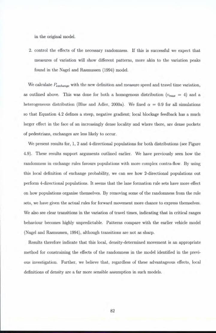
in the original model.

2. control the effects of the necessary randomness. If this is successful we expect that

measmes of variation will show different patterns, more akin to the variation peaks

found in the Nagel and Rasmussen (1994) model.

We calculate Pexchange with the new definition and measure speed and travel time variation,

as outlined above. This was done for both a homogenous distribution (vmax = 4) and a

heterogeneous distribution (Blue and Adler, 2000a). We fixed a = 0.9 for all simulations

so that Equation 4.2 defines a steep, negative gradient; local blockage feedback has a much

larger effect in the face of an increasingly dense locality and where there, are dense pockets

of pedestrians, exchanges are less likely to occur.

We present results for, 1, 2 and 4-directional populations for both distributions (see Figure

4.9). These results support arguments outlined earlier. We have previously seen how the

randomness in exchange rules favours populations with more complex contra-flow. By using

this local defirlltion of exchange probability, we can see how 2-directional populations out

perform 4-directional populations. It seems that the lane formation rule sets have more effect

on how populations organise themselves. By removing some of the randomness from the rule

sets, we have given the actual rules for forward movement more chance to express themselves.

We also see clear transitions in the variation of travel times, indicating that in critical ranges

behaviom becomes highly unpredictable. Patterns compare with the earlier vehicle model

(Nagel and Rasmussen, 1994), although transitions are not as sharp.

Results therefore indicate that this local, density-determined movement is an appropriate

method for constraining the effects of the randomness in the model identified in the previ

ous investigation. Further, we believe that, regardless of these advantageous effects, local

definitions of density are a far more sensible assumption in such models.

82

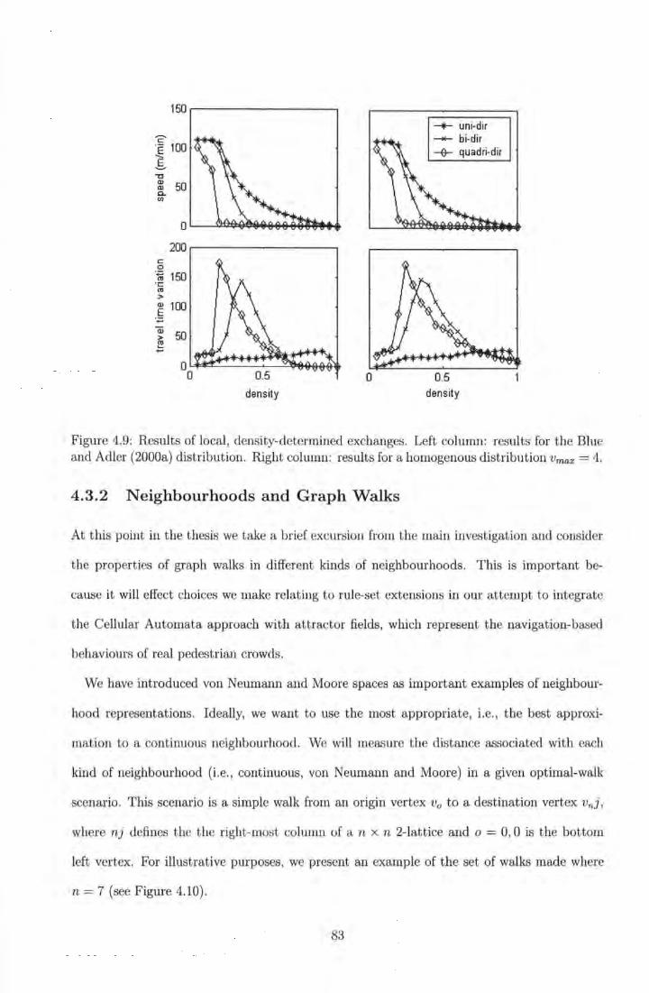
c ·E 100 g "'0

~ 50 a. (J)

OL-~~~~~~~·

~0 .-----------------, c 0

'fii 150 ·c (0

> Q) 100 E ·~

Qj 50 ~ -

0.5 density

0

-.+- uni-dir --- bi-dir + quadri-dir

0.5 density

Figure 4.9: Results of local, density-determined exchanges. Left column: results for the Blue and Adler (2000a) distribut ion. Right column: results for a homogenous distribution Vmax = 4.

4.3.2 Neighbourhoods and Graph Walks

At this point in the thesis we take a brief excursion from the main investigation and consider

the properties of graph walks in different kinds of neighbourhoods. This is important be-

cause it will effect choices we make relating to rule-set extensions in our attempt to integrate

the Cellular Automata approach with attractor fields, which represent the navigation-based

behaviours of real pedestrian crowds.

We have introduced von Neumann and Moore spaces as important examples of neighbour-

hood representations. Ideally, we want to use the most appropriate, i.e., the best approx.i-

mation to a continuous neighbourhood. We will measure the distance associated with each

kind of neighbourhood (i.e., continuous, von Neumann and Moore) in a given optimal-walk

scenario. This scenario is a simple walk from an origin vertex v0 to a destination vertex VnJ ,

where nj defines the the right-most column of a n x n 2-lattice and o = 0, 0 is the bottom

left vertex. For illustrative purposes, we present an example of the set of walks made where

n = 7 (see Figure 4.10).

83

•••••• ••••• •••• ••• •• •

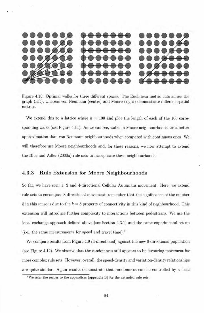
• ••••• • •••• • ••• • •• • • • Figure 4.10: Optimal walks for three different spaces. The Euclidean metric cuts across the graph (left), whereas von Neumann (centre) and Moore (right) demonstrate different spatial metrics.

We extend this to a lattice where n = 100 and plot the length of each of the 100 corre-

sponding walks (see Figure 4.11). As we can see, walks in Moore neighbourhoods are a better

approximation than von eumann neighbourhoods when compared with continuous ones. We

will therefore use Moore neighbourhoods and, for these reasons, we now attempt to extend

the Blue and Adler (2000a) rule sets to incorporate these neighbourhoods .

4.3.3 Rule Extension for Moore Neighbourhoods

So far , we have seen 1, 2 and 4-directional Cellular Automata movement. Here, we extend

rule sets to encompass 8-dircctional movement; remember that t he significance of the number

8 in this sense is due to the k = 8 property of connectivity in t his kind of neghbourhood. This

extension will int roduce further complexity to interactions between pedestrians. We use the

local exchange approach defined above (see Section 4.3.1) and the same experimental set-up

(i.e., the same measurements for speed and travel time).6

We compare results from Figure 4.9 ( 4-directional) against the new 8-directional popula tion

(see Figure 4.12). We observe that the randomness still appears to be favouring movement for

more complex rule sets. However, overall, the speed-density and variation-density relationships

are quite similar. Again results demonstrate that randomness can be controlled by a local

6We refer the reader to the appendices (appendix B) for the extended rule sets.

84

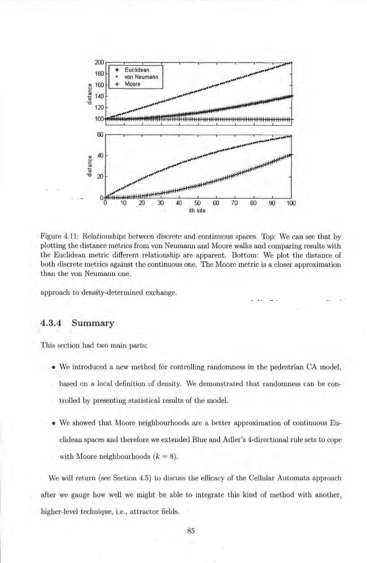
200

* Euclidean .,......,.

180 ......... • von Neumann ......... ... ...

~ 160 c: ~ 140 '0

120

100

60

<D 40 0 c: <11

iii '0 20

0

+ Moo re ...... ...... ........ ...... ...... ...... ...... ...... .... ~ ......

......... ...... ...... ......

...... ........ ......

... ...... .... .....

......

10 20 30 40 50 ith site

60 70

.........

........ _ ... -.........

80 90 100

Figure 4.11: Relationships between discrete and continuous spaces. Top: We can see that by plotting the distance metrics from von Neumann and Moore walks and comparing results with the Euclidean metric different relationship are apparent. Bottom: We plot the distance of both discrete metrics against the continuous one. The Moore metric is a closer approximation than the von Neumann one.

approach to density-determined exchange.

4.3.4 Summary

This section had two main parts:

• We introduced a new method for controlling randomness in the pedestrian CA model,

based on a local definition of density. We demonstrated that randomness can be con-

trolled by presenting statistical results of the model.

• We showed that Moore neighbourhoods are a better approximation of continuous Eu-

clidean spaces and therefore we extended Blue and Adler's 4-directional rule sets to cope

with Moore neighbourhoods (k = 8).

We will return (see Section 4.5) to discuss the efficacy of the Cellular Automata approach

after we gauge how well we might be able to integrate this kind of method with another,

higher-level technique, i. e., attractor fields.

85

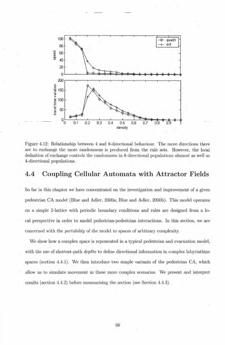
100

00 -c 60 Q) Q) Q.. (/) 40

20

0

200 c 0

'iii 150 ·~ > Q) 100 .§ Q)

50 > ~

0 0

density

Figure 4.12: Relationship between 4 and 8-directional behaviour. T he more directions there are to exchange the more randomness is produced from the rule sets. However, the local defini tion of exchange controls the randomness in 8-directionaJ populations alsmost as well as 4-directional populations.

4.4 Coupling Cellular Automata with Attractor Fields

So far in this chapter we have concentrated on the investigation and improvement of a given

pedestrian CA model (Blue and Adler, 2000a; Blue and Adler , 2000b). This model operates

on a simple 2-latt ice with periodic boundary condit ions and rules are designed from a lo-

cal perspective in order to model pedestrian-pedestrian interactions. In this section, we are

concerned with the portability of the model to spaces of arbit rary complexity.

We show how a complex space is represented in a typical pedestrian and evacuation model,

with the use of shortest-path depths to define directional information in complex labyrinthine

spaces (section 4.4.1). We then int roduce two simple variants of t he pedestrian CA, which

allow us to simulate movement in these more complex scenarios. We present and interpret

results (section 4.4.2) before summarising the section (see Section 4.4.3) .

86

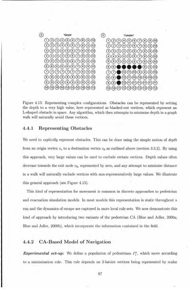
® ~· 00000®0®®@ 00000®0®®@ 00000®0®®@ 00000®0®®@ 00000®0®®@ ®®®®®®0®®@ 0000000®®@ ®®®®®®®®®@ ®®®®®®®®®@ @@@@@@@@@@

® 'Complex'

00000®0®®@ 00000®0®®@ 00000®0®®@ 00000®0®®@ 00000®0®®@ ®®·····®®@ 00. @@@®®®@ ®®e ®®®®®®® ®®e ®®®®®®® @@@@@'@@@@@

Figure 4.13: Represent ing complex configurations. Obstacles can be represented by setting the depth to a very high value, here represented as blacked-out vertices, which represent an L-shaped obstacle in space. Any algorithm, which then attempts to minimise depth in a graph walk will naturally avoid these vertices.

4.4.1 Representing Obstacles

We need to explicitly represent obstacles. This can be done using the simple notion of depth

from an origin vertex V0 to a destination vertex vd as outlined above (section 3.3.2). By using

this approach, very large values can be used to exclude certain vertices. Depth values often

decrease towards the exi t node vd, represented by zero, and any attempt to minimise distance

in a walk will naturally exclude vertices with non-representatively large values. We illustrate

this general approach (see Figure 4.13).

This kind of representation for movement is common in discrete approaches to pedestrian

and evacuation simulation models. In most models tllis representation is static throughout a

run and the dynamics of escape are captured in more local rule sets. We now demonstrate t ills

kind of approach by introducing two variants of t he pedestrian CA (Blue and Adler, 2000a;

Blue and Adler, 2000b) , which incorporate the information contained in the field .

4.4.2 CA-Based Model of Navigation

Experimental set-up: We define a population of pedestrians ~z, which move according

to a minimisation rule. This rule depends on 2-lattice vert ices being represented by scalar

87

•

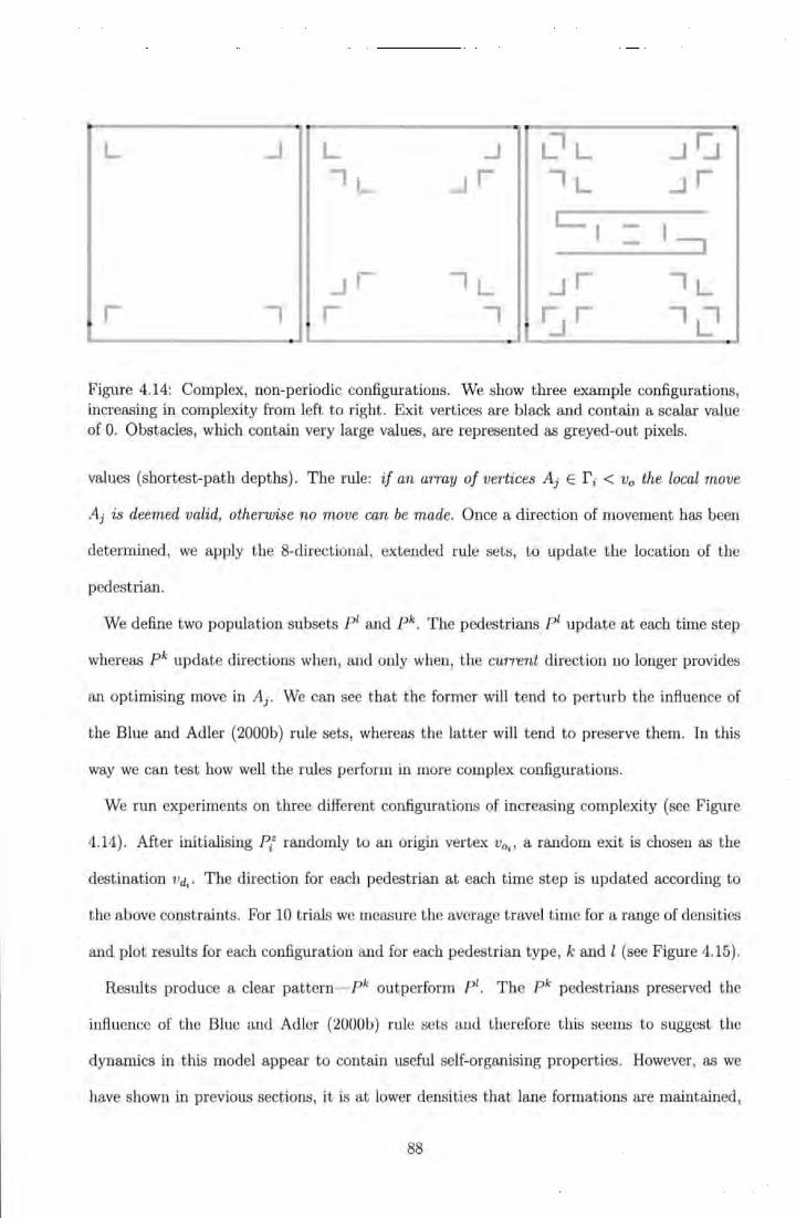
L ..J L ..J LIL ..Jr:.t ,L ...Jr ,L ..Jr

I I -- I::J

..Jr ,L ..Jr ,L r , r ,

~r ,Cl . Figure 4.14: Complex, non-periodic configurations. We show three example configurations, increasing in complexity from left to right. Exit vertices are black and contain a scalar value of 0. Obstacles, which contain very large values, are represented as greyed-out pixels.

values (shortest-path depths) . The rule: if an array of vertices Aj E r i < v0 the local move

Aj is deemed valid, otherwise no move can be made. Once a direction of movement has been

determined, we apply the 8-directional, extended rule sets, to update the location of the

pedestrian.

We define two population subsets P1 and pk . The pedestrians P1 update at each time step

whereas pk update directions when , and only when, the current direction no longer provides

an optimising move in Aj. We can see that the former will tend to perturb the influence of

the Blue and Adler (2000b) rule sets, whereas the latter will tend to preserve them. In this

way we can test how well the rules perform in more complex configurations.

We run experiments on three different configurations of increasing complexity (see Figure

4.14). After initialising P/ randomly to an origin vertex v0 il a random exit is chosen as the

destination vc4. The direction for each pedestrian at each t ime step is updated according to

the above constraints. For 10 trials we measure the average travel t ime for a range of densities

and plot results for each configuration and for each pedestrian type, k and l (see Figure 4. 15).

Results produce a clear pattern- Pk outperform P1. The pk pedestrians preserved the

influence of the Blue and Adler (2000b) rule sets and therefore t his seems to suggest the

dynamics in this model appear to contain useful self-organising properties. However, as we

have shown in previous sections, it is at lower densities that lane formations are maintained,

88

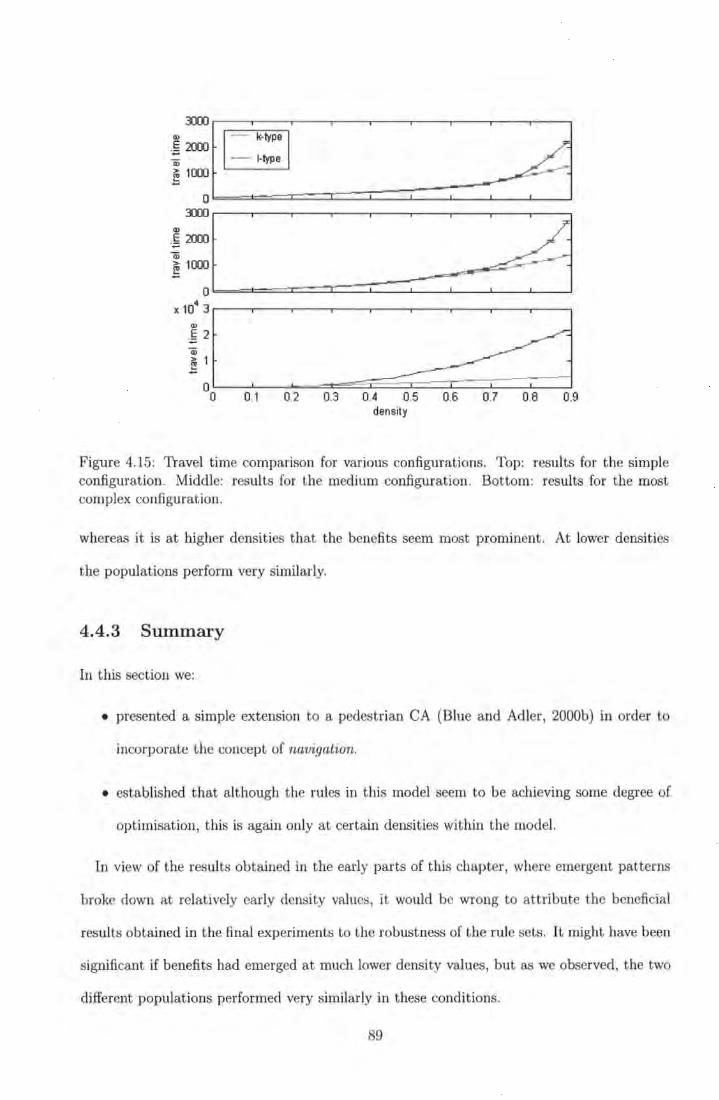
density

Figure 4.15: Travel time comparison for various configurations. Top: results for the simple configuration. Middle: results for the medium configuration. Bottom: results for the most complex configuration.

whereas it is at higher densities that the benefits seem most prominent. At lower densities

the populations perform very similarly.

4.4.3 Summary

In t his section we:

• presented a simple extension to a pedestrian CA (Blue and Adler, 2000b) in order to

incorporate t he concept of navigation.

• established that alt hough the rules in this model seem to be achieving some degree of

optimisation, this is again only a t certain densities within the model.

In view of the results obtained in the early parts of this chapter, where emergent patterns

broke down at relatively early density values, it would be wrong to attribute the beneficial

results obtained in the final experiments to the robust ness of the rule sets. It might have been

significant if benefits had emerged at much lower density values, but as we observed , the two

different populations performed very similarly in these conditions.

89

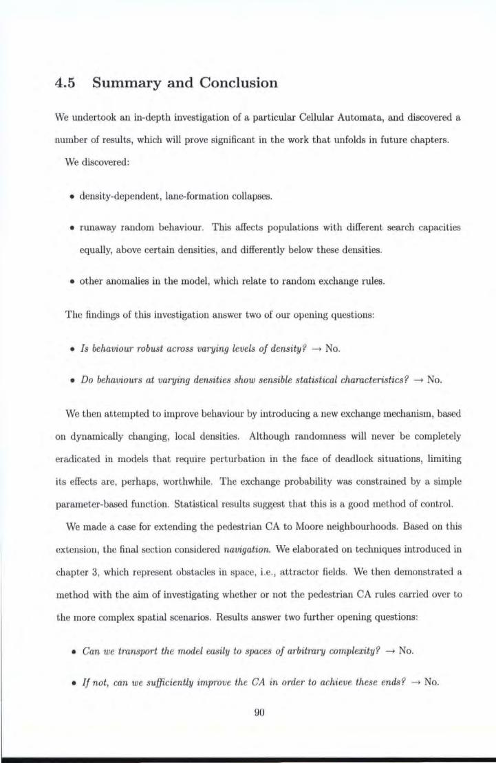
4.5 Summary and Conclusion

We undertook an in-depth investigation of a particular Cellular Automata, and discovered a

number of results, which will prove significant in the work that unfolds in future chapters.

We discovered:

• density-dependent, lane-formation collapses.

• runaway random behaviour. This affects populations with different search capacities

equally, above certain densities, and differently below these densities.

• other anomalies in the model, which relate to random exchange rules.

The findings of this investigation answer two of our opening questions:

• Is behaviour robust across varying levels of density? ---+ No.

• Do behaviours at varying densities show sensible statistical characteristics? ---+ No.

We then attempted to improve behaviour by introducing a new exchange mechanism, based

on dynamically changing, local densities. Although randomness will never be completely

eradicated in models that require perturbation in the face of deadlock situations, limiting

its effects are, perhaps, worthwhile. The exchange probability was constrained by a simple

parameter-based function. Statistical results suggest that this is a good method of control.

We made a case for extending the pedestrian CA to Moore neighbourhoods. Based on this

extension, the final section considered navigation. We elaborated on techniques introduced in

chapter 3, which represent obstacles in space, i.e., attractor fields. We then demonstrated a

method with the aim of investigating whether or not the pedestrian CA rules carried over to

the more complex spatial scenarios. Results answer two further opening questions:

• Can we transport the model easily to spaces of arbitrary complexity? ---+ No.

• If not, can we sufficiently improve the CA in order to achieve these ends? ---+ No.

90

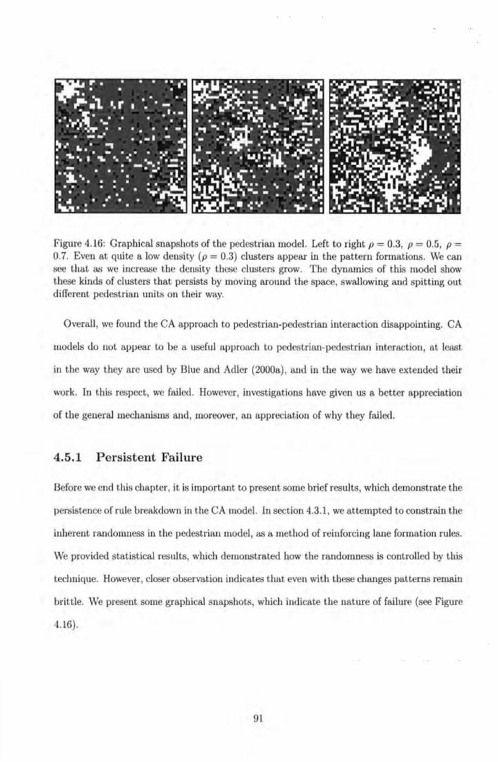
Figure 4.16: Graphical snapshots of the pedestrian model. Left to right p = 0.3, p = 0.5, p = 0.7. Even at quite a low density (p = 0.3) clusters appear in the pattern formations. We can see that as we increase the density these clusters grow. The dynamics of t his model show these kinds of clusters that persists by moving around the space, swallowing and spitting out different pedestrian units on their way.

Overall, we found the CA approach to pedestrian-pedestrian interaction disappointing. CA

models do not appear to be a useful approach to pedestrian-pedestrian interaction, at least

in the way they are used by Blue and Adler (2000a), and in the way we have extended their

work. In t his respect, we failed. However, investigations have given us a better appreciation

of the general mechanisms and, moreover, an appreciation of why they failed.

4.5.1 Persistent Failure

Before we end this chapter, it is important to present some brief results, which demonstrate the

persistence of rule breakdown in the CA model. In section 4.3.1, we attempted to constrain the

inherent randomness in the pedestrian model, as a method of reinforcing lane formation rules.

We provided statistical results, which demonstrated how the randomness is controlled by this

technique. However, closer observation indicates that even with these changes patterns remain

brittle. We present some graphical snapshots, which indicate the nature of failure (see Figure

4.16) .

91

~~-----· --r---~ +--• · l ·t · I· gap/eft

~

~ gap centre

)I

gapright

~

Figure 4.17: Components of search in CA models. The car CA (Nagel and Rasmussen, 1994) depends on search along a 1 - D component (!-lattice). We can see how the pedestrian CA (Blue and Adler, 2000a) adopts a similar method of search by decomposing a 2 - D space (2-lattice) into 1- D components.

4.5.2 Reasons for Failure

We believe that some of the problems of Blue and Adler's model stem from blindly inheriting

components from the car CA. Forward neighbourhood search in the car CA (Nagel and Ras-

mussen, 1994) is perfectly applicable to a one dimensional road scenario. However, because

Blue and Adler (2000a) adopt this kind of approach in a 2-D model, 2-D search becomes a

search along a collection of 1-D components (see Figure 4.17) .

We believe this choice severely limits the model. In the next chapter, we move attention

away from the logic of CA rules and focus on processes of search on 2-D graphs.

92

Chapter 5

Optimal Paths

In order to understand the sudden collapse of lane formation behaviour, we look at Boolean

percolation on the 2-lattice graph, and the formation of neighbourhood-connected clusters

(see Section 5.1). Statistical results suggest that Cellular Automata models are limited by

the fundamental properties of neighbourhood interactions, which catastrophically affect lo

cal dynamics. We therefore argue that an alternative approach to purely local dynamics is

required.

We then pause to list a number of essential levels of representation (see Section 5.2), before

introducing the Pulse Coupled Neural Network (PCNN), which provides a more inclusive

search than local neighbourhoods (see Section 5.3). Equation-based mechanisms are presented

in the context of image processing, the original application domain for the PCNN, and the

relevance of the PCNN to essential levels of representation are outlined (see Section 5.4). We

then discuss potential pitfalls in the PCNN, before improving it (see Section 5.5). Equations

are pruned in order to improve search robustness and behaviour is tested on simple and

complex 2-lattice configurations. Further definitions from graph theory are given, before a

chapter summary, where we recap on our main arguments (see Section 5.6).

93

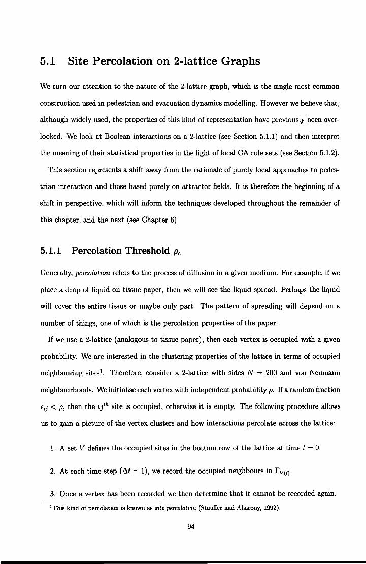
5.1 Site Percolation on 2-lattice Graphs

We turn our attention to the nature of the 2-lattice graph, which is the single most common

construction used in pedestrian and evacuation dynamics modelling. However we believe that,

although widely used, the properties of this kind of representation have previously been over

looked. We look at Boolean interactions on a 2-lattice (see Section 5.1.1) and then interpret

the meaning of their statistical properties in the light of local CA rule sets (see Section 5.1.2).

This section represents a shift away from the rationale of purely local approaches to pedes

trian interaction and those based purely on attractor fields. It is therefore the beginning of a

shift in perspective, which will inform the techniques developed throughout the remainder of

this chapter, and the next (see Chapter 6).

5.1.1 Percolation Threshold Pc

Generally, percolation refers to the process of diffusion in a given medium. For example, if we

place a drop of liquid on tissue paper, then we will see the liquid spread. Perhaps the liquid

will cover the entire tissue or maybe only part. The pattern of spreading will depend on a

number of things, one of which is the percolation properties of the paper.

If we use a 2-lattice (analogous to tissue paper), then each vertex is occupied with a given

probability. We are interested in the clustering properties of the lattice in terms of occupied

neighbouring sites1. Therefore, consider a 2-lattice with sides N = 200 and van Neumann

neighbourhoods. We initialise each vertex with independent probability p. If a random fraction

Eij < p, then the i}'h site is occupied, otherwise it is empty. The following procedure allows

us to gain a picture of the vertex clusters and how interactions percolate across the lattice:

1. A set V defines the occupied sites in the bottom row of the lattice at time t = 0.

2. At each time-step (t1t = 1), we record the occupied neighbours in fv(i)·

3. Once a vertex has been recorded we then determine that it cannot be recorded again.

1This kind of percolation is known as site percolation (Stauffer and Aharony, 1992).

94

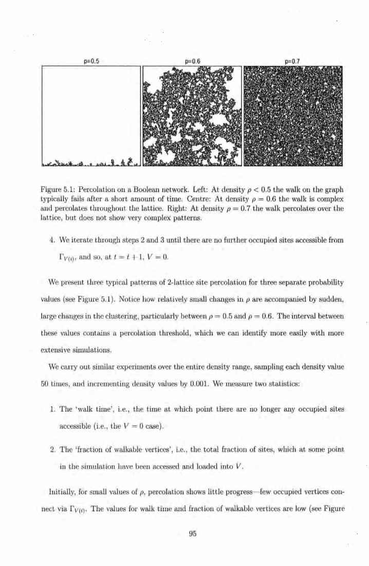
Figure 5.1: Percolation on a Boolean network. Left: At density p < 0.5 the walk on the graph typically fails after a short amount of time. Centre: At density p = 0.6 the walk is complex and percolates throughout the lattice. Right: At density p = 0.7 the walk percolates over the lattice, but does not show very complex patterns.

4. We iterate through steps 2 and 3 until there are no further occupied sites accessible from

rv(i) , and so, at t = t + 1, V = 0.

We present three typical patterns of 2-lattice site percolation for three separate probability

values (see Figure 5.1). Notice how relatively small changes in pare accompanied by sudden,

large changes in the clustering, particularly between p = 0.5 and p = 0.6. The interval between

these values contains a percolation threshold, which we can identify more easily with more

extensive simulations.

We carry out similar experiments over the entire density range, sampling each density value

50 times, and incrementing density values by 0.001. We measure two statistics:

1. The 'walk time', i.e. , the time at which point there are no longer any occupied sites

accessible (i.e., the V = 0 case).

2. The 'fraction of walkable vertices ', i.e., the total fraction of sites, which at some point

in the simulation have been accessed and loaded into V.

Initially, for small values of p, percolation shows little progress- few occupied vertices con-

nect via rv(i) · The values for walk time and fraction of walkable vertices are low (see Figure

95

~~--.---.---.---.---.---.----.---.---.--~

400

E3oo ·;:;

~ 200 ~

100

I •

o~--------~~~L_~--~~~_L__j

11) Q)

u "€ ~ 0.8 Q)

~ 0.6 ~

IV

~ 0.4 -0 ,

•• •• ~ 0.2

·~

~ o'----------!l!!f!I!~~--L----L--....1-_ _j - 0 0.1 0.2 0.3 0.4 0.5 0.6 0. 7 0.8 0.9

density (p)

Figure 5.2: Critical percolation transitions. Top: Sharp increases are produced within a given interval (p ~ 0.57 - 0.59) , which corresponds to the regime where clusters are complex (see Figure 5.1).

5.2) . However, in a critical range, we observe a sudden increases in the values for both statis-

tics. 2

5.1.2 Pc= Implications

Remember, for the pedestrian CA (Blue and Adler, 2000a), we observed fairly sudden changes

in behaviour at certain density ranges (p ~ 0.3). The significance of percolation thresholds to

pedestrian models are as follows. To initialise a graph with pedestrians is a Boolean operation

because we either place a pedestrian on a vertex or we don't. In this way, all models that use

this kind of spatial representation implement a type of Boolean network.

We believe that the results in the previous chapter, where behaviours were observed to

suddenly collapse, rather than progressively deteriorate, are the result of unwanted interaction,

between neighbourhoods, when they suddenly become connected. In the Blue and Adler

(2000a) model, neighbourhood search is defined by a number of variables (gapleft , gapright ,

2With similar kinds of experiments for lattices with very large N it has been shown that the critical point Pc= 0.59275 (Stauffer and Aharony, 1992; Sole and Goodwin, 2000).

96

gapcentre• Vmax), rather than a von Newnann neighbourhood, but according to the statistical

properties of the 2-lattice, we should expect sudden, giant-component connections, regardless

of neighbourhood type. We believe that the 1-D components in the Blue and Adler (2000a}

model are perturbed by the updates of other pedestrians in the lattice. Therefore, when

pedestrians join hands and cluster, a single pedestrian move might have effects far beyond

the dynamics of its own locality in a single update of the entire population.

In this way, pedestrian updates become limited by a complex, interactive web of overlapping

neighbourhoods. For this reason, any self-organising properties of local rules have less effect on

the dynamics in the face of increasing density. Such localities therefore make it very difficult

to implement sensible behaviours in higher-density regimes.

In order to further demonstrate the significance of the above argument, we illustrate regimes

in CA behaviour, which we think correspond to different regimes of percolation (see Figure 5.3,

Top). Notice how clusters begin to form in the CA at the point where giant clusters emerge

in the boolean network. We also present results for the travel time variation of pedestrians

and see that variations for different populations converge within the critical range where a

transition in the cluster size is observed. These results lend significant weight to the idea that

local rules in CA models get invaded by giant component networks, which then dominate the

dynamics of the model.

5.2 Important Representations

This part of the thesis defines a point of departure from some of the methods that are currently

used within the field of pedestrian and evacuation dynamics. In the light of observation made

thus far, we move our attention away from the work of others, and begin the development of

an alternative approach.

We will begin by providing a summary of what we believe are important representations

that need to be incorporated into our methods. These should be thought of as related and

interdependent objectives, which will determine the nature of the methods we develop.

97

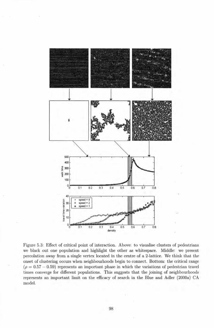
~.---.---.----.---.------~n----.~~

400

~:m ~200 l

100

0o~--0~.1--~0.~2 --~0~.3--~0.~4~~0~.5~~0.6~~0~.7---0~.8

density

Figure 5.3: Effect of critical point of interaction. Above: to visualise clusters of pedestrians we black out one population and highlight the other as whitespace. Middle: we present percolation away from a single vertex located in the centre of a 2-lattice. We think that the onset of clustering occurs when neighbourhoods begin to connect. Bottom: the critical range (p = 0.57- 0.59) represents an important phase in which the variations of pedestrian travel t imes converge for different populations. This suggests that the joining of neighbourhoods represents an important limit on the efficacy of search in t he Blue and Adler (2000a) CA model.

98

The following four levels are important:

1. Inclusive search: So far in this thesis we have covered a. number of techniques, which

rely on the concept of search--e.g., the pedestrian CA (Blue and Adler, 2000a.) and the

Space Syntax approach {Penn and Turner, 2002) and we have identified serious problems

with both. The basis of our first criterion is that a search algorithm needs to cover an

appropriate local region in order to obtain information from the environment, which

allows effective dynamics to be specified. A more inclusive search is therefore required.

2. Local dynamics: The reason we need an inclusive search is to find the appropriate vectors

of the lattice to cancel. Only when a more inclusive search has been made is this possible.

For example, if we only search a subset of vertices in a. neighbourhood, then we might be

missing essential information. The problem here is again to capture enough information,

so that appropriate local dynamics can be specified. We need to produce an algorithm,

which can effectively and efficiently compute local moves and model emergent patterns

found in real crowds.

3. Local-global linking: Using the established attractor field approach guarantees that there

is a path, leading from any given origin vertex, to an exit vertex. However, we cannot

guarantee that a pedestrian will follow a path, which is simultaneously sensitive to local

conditions and longer-range destinations. Therefore, there must be some inherent linkage

between the current local situation of the pedestrian, i.e., its origin v0 , its neighbourhood

r v(o)• and the exit or destination vertex vd, which will often be a much longer-range

target.

4. Pedestrian and obstacle representations: Finally, within the context of these criteria,

it is important to incorporate representations for other pedestrians and obstacles that

define a configuration.

We now introduce the Pulse Coupled Neural Network, which we believe to be an appropriate

search algorithm in the light of the above requirements.

99

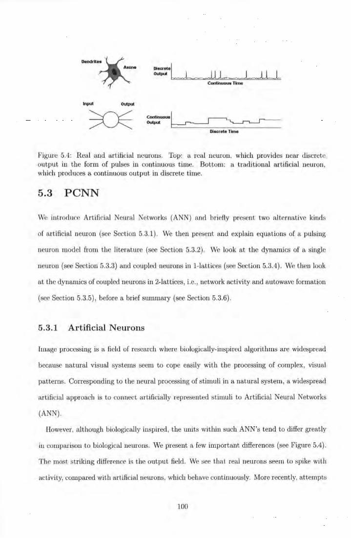
Dendrtt~AKo -~-

Input Output

~.!tnuous

Discrete Time

Figure 5.4: Real and artificial neurons. Top: a real neuron, which provides near discrete output in the form of pulses in continuous time. Bottom: a traditional artificial neuron, which produces a continuous output in discrete time.

5.3 PCNN

We introduce Artificial Neural etworks (ANN) and briefly present two alternative kinds

of art ificial neuron (see Section 5.3.1). We then present and explain equations of a pulsing

neuron model from the literature (see Section 5.3.2). We look at the dynamics of a single

neuron (see Section 5.3.3) and coupled neurons in 1-lattices (see Section 5.3.4). We then look

at the dynamics of coupled neurons in 2-lattices, i.e., network activity and autowave formation

(see Section 5.3.5) , before a brief summary (see Section 5.3.6).

5. 3.1 Artificial Neurons

Image processing is a field of research where biologically-inspired algorithms are widespread

because natural visual systems seem to cope easily with the processing of complex, visual

patterns. Corresponding to the neural processing of stimuli in a natural system, a widespread

artificial approach is to connect artificially represented stimuli to Artificial Neural Networks

(ANN).

However, although biologically inspired, the units within such ANN's tend to differ greatly

in comparison to biological neurons. We present a few important differences (see Figure 5.4).

The most striking difference is t he output field. We see that real neurons seem to spike with

activity, compared with artificial neurons, which behave continuously. More recently, attempts

100

are being made to model spiking behaviour, and many examples of these pulsed neurons now

exist (e.g., Maass and Bishop, 1998).

Another example is the Pulse-Coupled Neuron, which was first developed on the basis of

observations into the mammalian visual system, before being adapted to problems of machine

vision (Lindblad and Kinser, 1998). Instead of relying on the adaptation of weighed links

to training patterns, as is common with traditional ANN, the pulsed-coupled neuron is an

attempt to model spiking behaviour, and exploit patterns of spike synchronisation in neural

populations.

We introduce the PCNN in its original image processing context for two reasons. Firstly,

the mechanics of the algorithm are better understood in the context of an application. Second,

this application requires a similar structure of equations and forms a good basis to explain

how the network can be used to search in 2-lattice spaces.

5.3.2 Pulsed Neuron Model

The computational engine relies on local couplings, various kinds of feedback, and stimulation

from external pixels in an image plane. This image plane maps to a neural plane, which is a

matrix of artificial units. The following equations describe a single, matrix-embedded neuron

(Scharnschula, Johnson and lnguva, 2000):

F;;(t) = e-apAtF;;(t- 1) + S;; + L wijklykl(t-1)

kl

L;;(t) = e-hAt L;;(t- 1) + L M;;kt Ykl(t-1)

kl

U;;(t) = F;;(t){1 + (JL1;(t))

_ { 1 if U1;(t) > 8;;(t) Y;;(t) -

0 otherwise

101

(5.1)

(5.2)

(5.3)

(5.4)

(5.5)

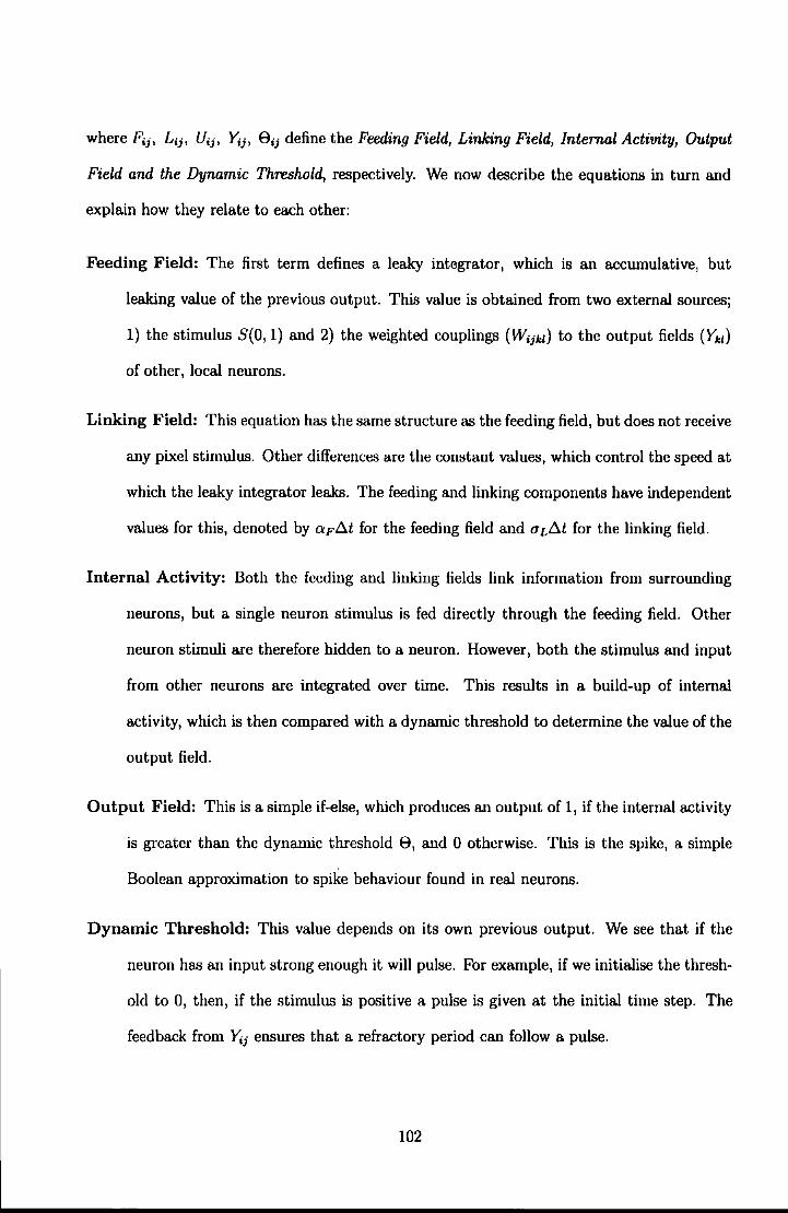
where F;j I L;j I U;j I Y;j I eij define the Feeding Field, Linking Field, Internal Activity, Output

Field and the Dynamic Threshold, respectively. We now describe the equations in turn and

explain how they relate to each other:

Feeding Field: The first term defines a leaky integrator, which is an accumulative, but

leaking value of the previous output. This value is obtained from two external sources;

1) the stimulus S(O, 1) and 2) the weighted couplings (W;jiu) to the output fields (Ykt)

of other, local neurons.

Linking Field: This equation has the same structure as the feeding field, but does not receive

any pixel stimulus. Other differences are the constant values, which control the speed at

which the leaky integrator leaks. The feeding and linking components have independent

values for this, denoted by OtFf:::..t for the feeding field and aLf:::..t for the linking field.

Internal Activity: Both the feeding and linking fields link information from surrounding

neurons, but a single neuron stimulus is fed directly through the feeding field. Other

neuron stimuli are therefore hidden to a neuron. However, both the stimulus and input

from other neurons are integrated over time. This results in a build-up of internal

activity, which is then compared with a dynamic threshold to determine the value of the

output field.

Output Field: This is a simple if-else, which produces an output of 1, if the internal activity

is greater than the dynanlic threshold 8, and 0 otherwise. Tllis is the spike, a simple

Boolean approximation to spike behaviour found in real neurons.

Dynamic Threshold: This value depends on its own previous output. We see that if the

neuron has an input strong enough it will pulse. For example, if we initialise the thresh

old to 0, then, if the stimulus is positive a pulse is given at the initial time step. The

feedback from Y;i ensures that a refractory period can follow a pulse.

102

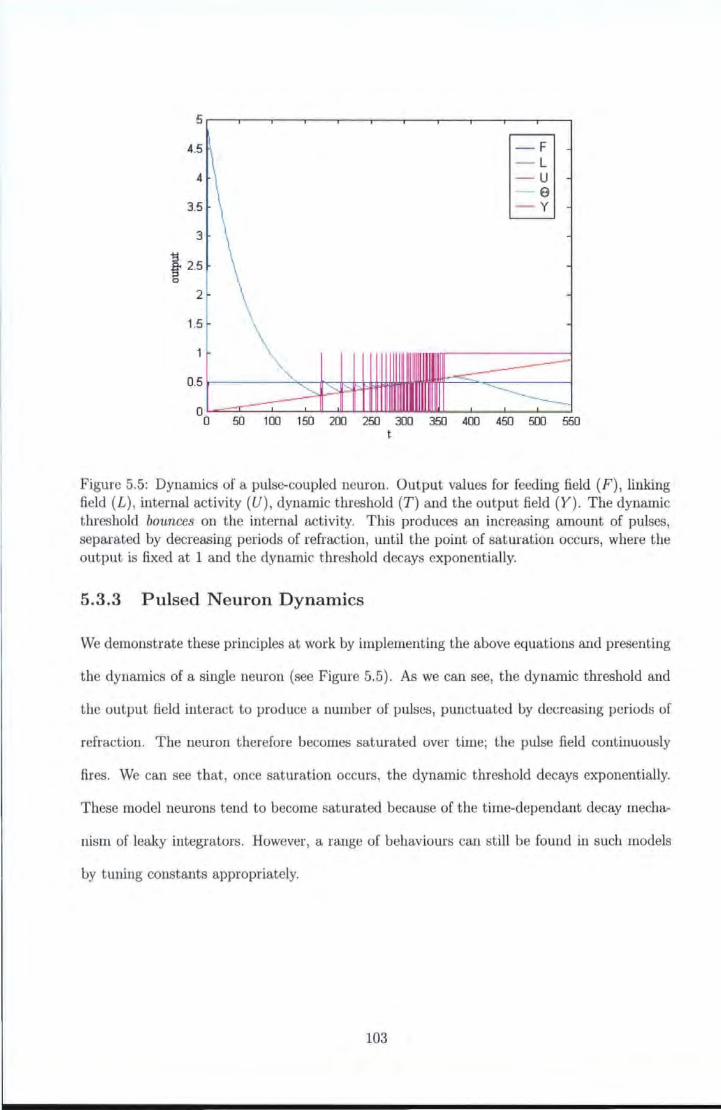
5

4.5 - F - L

4 - u - 9

3.5 - Y

3

E. 2.5 :::3 0

2

1.5

50 1 DO 150 200 250 300 350 400 450 500 550 t

Figure 5.5: Dynamics of a pulse-coupled nemon. Output values for feeding field (F), linking field (£) , internal activity (U), dynamic threshold (T) and the output field (Y). The dynamic threshold bounces on the internal activity. This produces an increasing amount of pulses, separated by decreasing periods of refraction , until the point of saturation occurs, where the output is fixed at 1 and the dynamic threshold decays exponentially.

5.3.3 Pulsed Neuron Dynamics

We demonstrate these principles at work by implementing the above equations and presenting

the dynamics of a single neuron (see Figure 5.5). As we can see, the dynamic threshold and

the output field interact to produce a number of pulses, punctuated by decreasing periods of

refraction. The neuron therefore becomes saturated over time; the pulse field continuously

fires. We can see that, once saturation occurs, the dynamic threshold decays exponentially.

These model neurons tend to become saturated because of the time-dependant decay mecha-

nism of leaky integrators. However, a range of behaviours can still be found in such models

by tuning constants appropriately.

103

t=l

t=2

t=3

t=4

t=S

Figure 5.6: Autowaves in non-periodic, 1-lattice media. Two autowaves are presented. Left: a !-directional autowave. Right: a 2-directional autowave, which departs from a given origin and travels in opposite directions.

5.3.4 Pulse-Coupled Dynamics: 1-lattice

An interesting property of networked artificial neurons, if parameters are set to appropriate

values, is t he occurrence of a series of spikes, which travel away from the source neuron. This

series is known as an autowave. This directional transmission of spikes is made possible by

the refractory period, which as we have seen, prevents the neuron from spiking immediately

after it has done so.

In order to observe autowave formation, we implement a non-periodic 1-lattice network of

neurons N with immediate local connections ( k = 2, and k = 1 at the boundary) . We present

results of two simple simulations in a space-time diagram (see Figure 5.6). In the first example,

we provide input to NI. At t = 2, the boundary demands that only N2 receives input from

NI, which enters a refractory period, while N2 processes the input received form N1 . At all

time steps each neuron that pulses enters a refractory period and therefore the spikes produce

a clear wave, which travels through each neuron left to right in 5 = 1 + 1 + 1 + 1 + 1 t ime-steps.

In the second example, we provide input to N3. T he boundary does not interfere with this

neuron and the wave travels in opposite directions away from N3 . The wave travels t hrough

each neuron in 3 = 1 + ( 4/2) time-steps.

104

5.3.5 P ulse-Coupled Dynamics: 2-lattice

5.3.5.1 Neighbourhood radius

We organise a 2-lattice network of neurons with Moore neighbourhood r connections so k = 8.

The radius r of a neighbourhood would increase the computational load on the network-e.g.,

with r = 2, the number of connections goes from 8 to 24 = (8 + 16), capturing the immediate

Moore neighbourhood r(S) of a subgraph S(G) = r. However, for our application we only

use neighbourhoods where r = 1. 3

5.3.5.2 Use of Weights

Most neural networks are associated with the idea of weighted inputs. With a traditional

ANN, it is common that the network has a random set of initial weights, which are then

trained. For example, with the Multi-Layered-Perceptron, test data is presented and training

data is attached to the network to help calculate a network error. This error is then propagated

back through the network and weights are adjusted to some degree in order to minimise error.

This general process of training is repeated until the error of the network is sufficiently low;

i.e., until the distributed encoding in the weights contains a sufficient representation of the

training data.

The use of weights in the PCNN is totally different. Here the idea of training is irrelevant.

We only consider a predefined set of weights, which then remain fixed throughout a run. The

weights used for the current project are simple 1/r connections. The further out a neuron

is from the centre neuron, the less weight it will have on the behaviour. However, because

our radius r = 1, we see that the weights Wiikl = r = 1. As long as there are couplings, the

relationships between the various equations produce self-organising, interactive behaviours.

3For more information on details of r for different applications see (Lindblad and Kinser, 1998}.

105

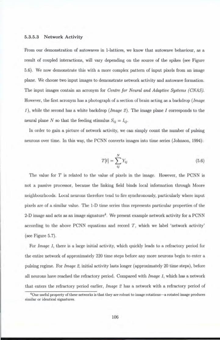
5.3.5.3 Network Activity

From our demonstration of autowaves in 1-lattices, we know that autowave behaviour, as a

result of coupled interactions, will vary depending on the source of the spikes (see Figure

5.6) . We now demonstrate this with a more complex pattern of input pixels from an image

plane. We choose two input images to demonstrate network activity and autowave formation .

The input images contain an acronym for Centre for Neural and Adaptive Systems (CNAS).

However, the first acronym has a photograph of a section of brain acting as a backdrop (Image

1 ), while the second has a white backdrop (Image 2) . The image plane I corresponds to the

neural plane N so that the feeding stimulus Sij = Iij·

In order to gain a picture of network activity, we can simply count the number of pulsing

neurons over time. In this way, the PCNN converts images into time series (Johnson, 1994):

N

T[t] = Ll'ij (5.6) ij

The value for T is related to the value of pixels in the image. However, the PCNN is

not a passive processor, because the linking field binds local information through Moore

neighbourhoods. Local neurons therefore tend to fire synchronously, particularly where input

pixels are of a similar value. The 1-D t ime series thus represents particular properties of the

2-D image and acts as an image signature4 . We present example network activity for a PCNN

according to the above PCNN equations and record T , which we label 'network activity'

(see Figure 5.7).

For Image 1, there is a large initial activity, which quickly leads to a refractory period for

the entire network of approximately 220 time steps before any more neurons begin to enter a

pulsing regime. For Image 2, initial activity lasts longer (approximately 20 time steps) , before

all neurons have reached the refractory period. Compared with Image 1, which has a network

that enters the refractory period earlier, Image 2 has a network with a refractory period of

40ne useful property of these networks is that they are robust to image rotations-a rotated image produces similar or identical signatures.

106

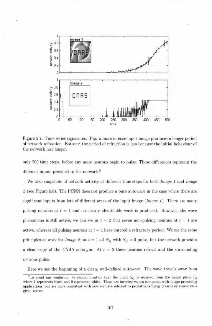
>-> 0.8 .t:< >

-~ 0.6 .::.:. 1 0.4

~ 0.2

-~0.8 .i!!: ~ 0.6 ~ ~ 0.4 a; c 0.2

50 1 00 150 200 250 l10 350 400 450 500 time

Figure 5.7: Time series signatures. Top: a more intense input image produces a longer period of network refraction. Bottom: the period of refraction is less because the init ial behaviour of the network last longer.

only 200 t ime steps, before any more neurons begin to pulse. These differences represent the

different inputs provided to the network.5

We take snapshots of network activity at different t ime steps for bot h Image 1 and Image

2 (see Figure 5.8) . The PCNN does not produce a pure autowave in the case where there are

significant inputs from lots of different areas of the input image (Image 1 ). There are many

pulsing neurons at t = 1 and no clearly identifiable wave is produced. However, t he wave

phenomena is still active; we can see at /, = 2 that seven non-pulsing neurons at f. = 1 are

active, whereas all pulsing neurons at t = 1 have entered a refractory period. We see the same

principles at work for Image 2; at t = 1 all Nii with Sii > 0 pulse, but the network provides

a clean copy of the CNAS acronym. At t = 2 these neurons refract and the surrounding

neurons pulse.

Here we see the beginning of a clean, well-defined autowave. The wave travels away from

5To avoid any confusion, we should ment ion that the input S;; is received from the image plane ! ;; where 1 represents black and 0 represents white. These are inverted values compared with image processing applications, but are more consistent with how we have referred to pedestrians being present or absent on a given vertex.

107

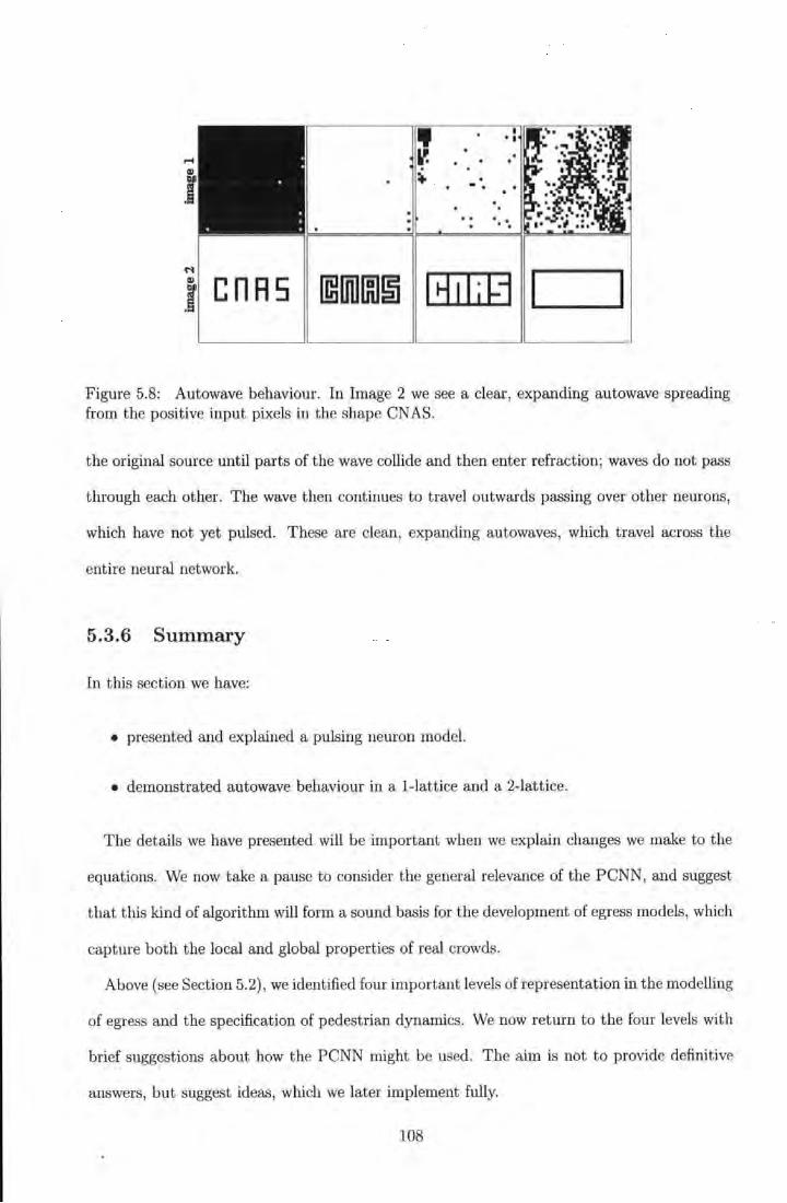
cnRs

. -.

Figure 5.8: Autowave behaviour. In Image 2 we see a clear, expanding autowave spreading from the positive input pixels in the shape CN AS.

the original source until parts of the wave collide and then enter refraction; waves do not pass

through each other . The wave then cont inues to t ravel outwards passing over other neurons,

which have not yet pulsed. These are clean, expanding autowaves, which travel across the

entire neural network.

5.3.6 Summary

In this section we have:

• presented and explained a pulsing neuron model.

• demonstrated autowave behaviour in a 1-lattice and a 2-lattice.

The details we have presented will be important when we explain changes we make to the

equations. We now take a pause to consider the general relevance of the PCNN, and suggest

that t his kind of algorithm will form a sound basis for the development of egress models, which

capture both the local and global properties of real crowds.

Above (see Section 5.2) , we identified four important levels of representation in the modelling

of egress and the specification of pedestrian dynamics. We now return to the four levels with

brief suggestions about how the PCNN might be used. The aim is not to provide definitive

answers, but suggest ideas, which we later implement fully.

108

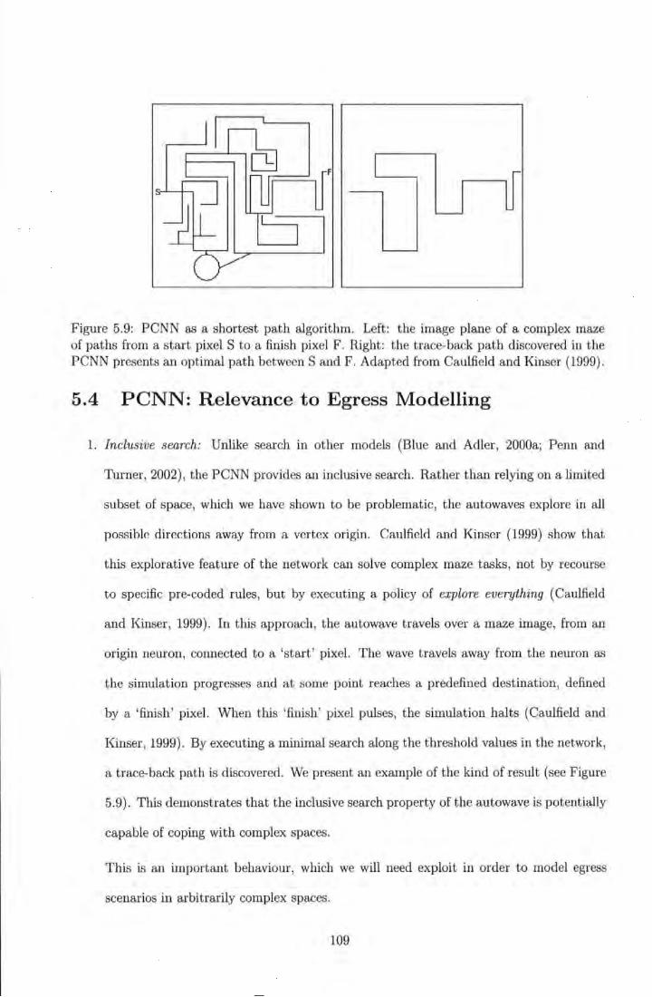
l - _j l

Figure 5.9: PCNN as a shortest path algorithm. Left: the image plane of a complex maze of paths from a start pixel S to a finish pixel F. Right: the trace-back path discovered in the PCNN presents an optimal path between Sand F. Adapted from Caulfield and Kinser (1999).

5.4 PCNN: Relevance to Egress Modelling

1. Inclusive search: Unlike search in other models (Blue and Adler, 2000a; Penn and

Thrner, 2002) , the PCNN provides an inclusive search. Rather than relying on a limited

subset of space, which we have shown to be problematic, the autowaves explore in all

possible directions away from a vertex origin. Caulfielrl and Kinser (1999) show that

this explorative feature of the network can solve complex maze tasks, not by recourse

to specific pre-coded rules, but by executing a policy of explore everything (Caulfield

and Kinser, 1999). In this approach, the autowave travels over a maze image, from an

origin neuron, connected to a 'start ' pixel. The wave travels away from the neuron as

the simulation progresses and at some point reaches a predefined destination, defined

by a ' finish' pixel. When this 'finish pixel pulses, the simulation halts (Caulfield and

Kinser, 1999). By executing a minimal search along the threshold values in the network,

a trace-back path is discovered. We present an example of the kind of result (see Figure

5.9) . This demonstrates that the inclusive search property of the autowave is potentially

capable of coping with complex spaces.

This is an important behaviour, which we vrill need exploit in order to model egress

scenarios in arbitrarily complex spaces.

109

2. Local dynamics: As autowave search moves away from a vertex origin, we will be able

to specify occupied pedestrian vertices as the source of autowaves. In this way, local

dynamics may be captured during the initial stages of search as the wave progresses

through different regions.

3. Local-global linking: We will also be able to specify at which vertex a destination is

set. In this way, we will be able to combine the longer-range process of egress with local

pedestrian dynamics. The distinction between local and global is merged with the image

of an expanding autowave.

We will therefore need to ask ourselves at what point in autowave search we apply local

rules. We showed earlier that dynamics in localities are brittle on 2-lattice spaces. One

aim will be to develop a more robust method.

4. Pedestrian and obstacle representations: We have seen above that the PCNN behaves

through the synchronization of spikes. This boolean approximation should be very useful

for our purposes. We will see in the next section how this behaviour allows a simple

approach to the specification of dynamics, which include configurational and pedestrian

obstacles.

The following section is intended to demonstrate the use of autowave search, and provide

details of techniques, which implement ideas we have suggested here. We will concentrate on

relatively simple scenarios, but will build upon them later in the thesis (see Chapter 6).

5.5 Robust Autowaves

Firstly, we consider the possible pitfalls of the PCNN equations for our own domain of appli

cation (see Section 5.5.1), and then prune equations to improve search robustness {see Section

5.5.2). Then, as a precursor to how they might be used to model pedestrian navigation,

we demonstrate explorative behaviour of the new equations in complex spaces and relate

behaviour to further definitions in Graph Theory (see Section 5.5.3).

110

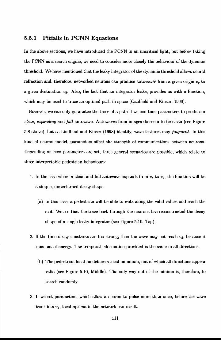
5.5.1 Pitfalls in PCNN Equations

In the above sections, we have introduced the PCNN in an uncritical light, but before taking

the PCNN as a search engine, we need to consider more closely the behaviour of the dynamic

threshold. We have mentioned that the leaky integrator of the dynamic threshold allows neural

refraction and, therefore, networked neurons can produce autowaves from a given origin V0 to

a given destination vd. Also, the fact that an integrator leaks, provides us with a function,

which may be used to trace an optimal path in space (Caulfield and Kinser, 1999).

However, we can only guarantee the trace of a path if we can tune parameters to produce a

clean, expanding and full autowave. Autowaves from images do seem to be clean (see Figure

5.8 above), but as Lindblad and Kinser (1998) identify, wave features may fragment. In this

kind of neuron model, parameters affect the strength of communications between neurons.

Depending on how parameters are set, three general scenarios are possible, which relate to

three interpretable pedestrian behaviours:

1. In the case where a clean and full autowave expands from V0 to vd, the function will be

a simple, unperturbed decay shape.

(a) In this case, a pedestrian will be able to walk along the valid values and reach the

exit. We see that the trace-back through the neurons has reconstructed the decay

shape of a single leaky integrator (see Figure 5.10, Top).

2. If the time decay constants are too strong, then the wave may not reach vd, because it

runs out of energy. The temporal information provided is the same in all directions.

(b) The pedestrian location defines a local minimum, out of which all directions appear

valid (see Figure 5.10, Middle). The only way out of the minima is, therefore, to

search randomly.

3. If we set parameters, which allow a neuron to pulse more than once, before the wave

front hits vd, local optima in the network can result.

111

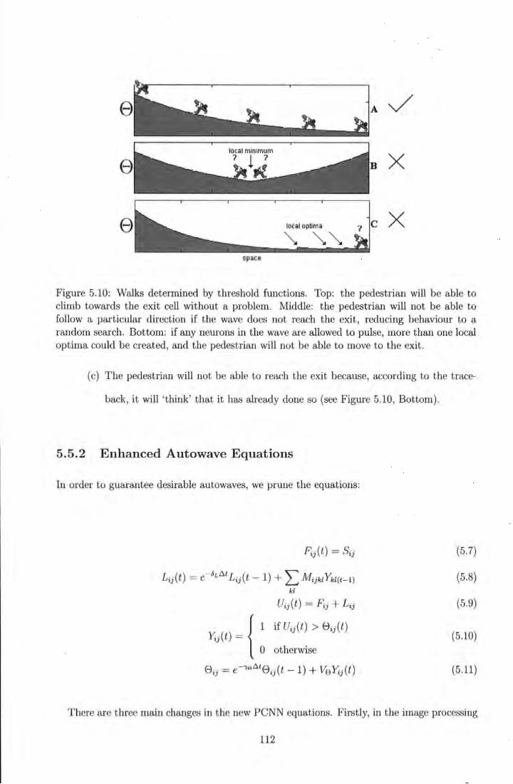
e

e

local optima

~ ~~ X e

space

Figure 5.10: Walks determined by threshold functions. Top: the pedestrian will be able to climb towards the exit cell without a problem. Middle: the pedestrian will not be able to follow a particular direction if the wave does not reach the exit, reducing behaviour to a random search. Bottom: if any neurons in the wave are allowed to pulse, more than one local optima could be created, and the pedestrian will not be able to move to the exit.

(c) The pedestrian will not be able to reach the exit because, according to the trace-

back, it will ' think' that it has already done so (see Figure 5.10, Bottom).

5.5.2 Enhanced Autowave Equations

In order to guarantee desirable autowaves, we prune the equations:

L1i(t) = e-ht:.t Lii(t - 1) + L MijktYkt(t- 1) kl

Uii(t) = Fii + Lii

Y;;(t) = { : otherwise

(5.7)

(5.8)

(5.9)

(5.10)

(5.11)

There are three main changes in the new PCNN equations. Firstly, in the image processing

112

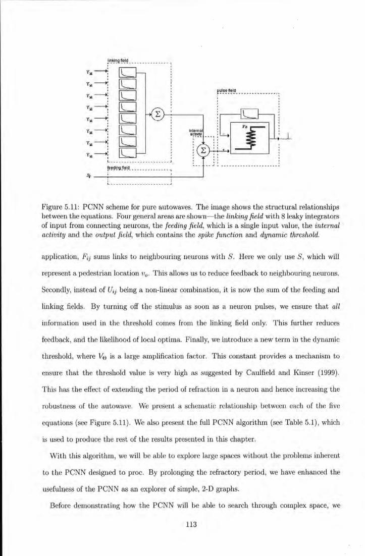
~'!~'!!!. ~1!_1~- - - - - - -- - - - - - - - ,

yil~ ' D ykl------+: ' [0 y)d--+: ' [0 y ---+: il ' ' ' [0 y --+• il : ' [0 Yu --+: ' [0 yil--+: I

' yil --+:

I

L------------------ ----J (!!~~i!lJI_fiJILd _______________ ,

~~~~~ ~~~~- -- -- ---- --- --- .. . ' ' ' ' ' '

Internal : a;~tt ___ , : -

' ' '' ' ' : L r-+-' +-' ..i..+._ ___ _. ' '' '' '' ' o I I 1 .. __ -- ~ .. _____________________ ..

~--~--------------~----~ . . . ' L---- ------------------J

Figure 5.11: PCNN scheme for pure autowaves. The image shows the structural relationships between the equations. Four general areas are shown-the linking field with 8leaky integrators of input from connecting neurons, the f eeding field, which is a single input value, the internal activity and the output field, which contains the spike function and dynamic threshold.

application, Fij sums links to neighbouring neurons with S. Here we only use S, which will

represent a pedestrian location V 0 • This allows us to reduce feedback to neighbouring neurons.

Secondly, instead of Uij being a non-linear combination, it is now the sum of the feeding and

linking fields. By turning off the stimulus as soon as a neuron pulses, we ensure that all

information used in the threshold comes from the linking field only. This further reduces

feedback, and the likelihood of local optima. Finally, we introduce a new term in the dynamic

threshold, where Ve is a large amplification factor. This constant provides a mechanism to

ensure that the threshold value is very high as suggested by Caulfield and Kinser (1999).

This has the effect of extending the period of refraction in a neuron and hence increasing the

robustness of the autowave. We present a schematic relationship between each of the five

equations (see Figure 5.11). We also present the full PCNN algorithm (see Table 5.1), which

is used to produce the rest of the results presented in this chapter.

With tllis algorithm, we will be able to explore large spaces without the problems inherent

to the PCNN designed to proc. By prolonging the refractory period, we have enhanced the

usefulness of the PCNN as an explorer of simple, 2-D graphs.

Before demonstrating how the PCNN will be able to search through complex space, we

113

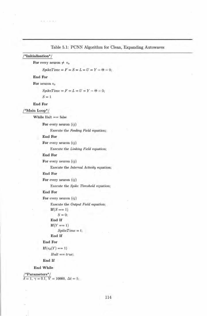
Table 5.1: PCNN Algorithm for Clean, Expanding Autowaves

/*Initialisation*/

For every neuron ;f= V 0

SpikeTime = F = S = L = U = Y = 9 = 0;

End For

For neuron V0

SpikeTime = F = L = U = Y = 9 = 0;

8=1

End For

/*Main Loop*/

While Halt == false

For every neuron (ij)

Execute the Feeding Field equation;

End For

For every neuron ( ij)

Execute the Linking Field equation;

End For


Execute the Internal Activity equation;

End For


Execute the Spike Threshold equation;

End For


Execute the Output Field equation;

lf(S == 1) 8=0;

End If

lf(Y == 1) SpikeTime = t ;

End If

End For

If(vd(Y) == 1)

Halt == true;

End If

End While

/*Parameters*/ (5 = 1, 'Y = 0.1 , V= 10000, f::l.t = 1;

114

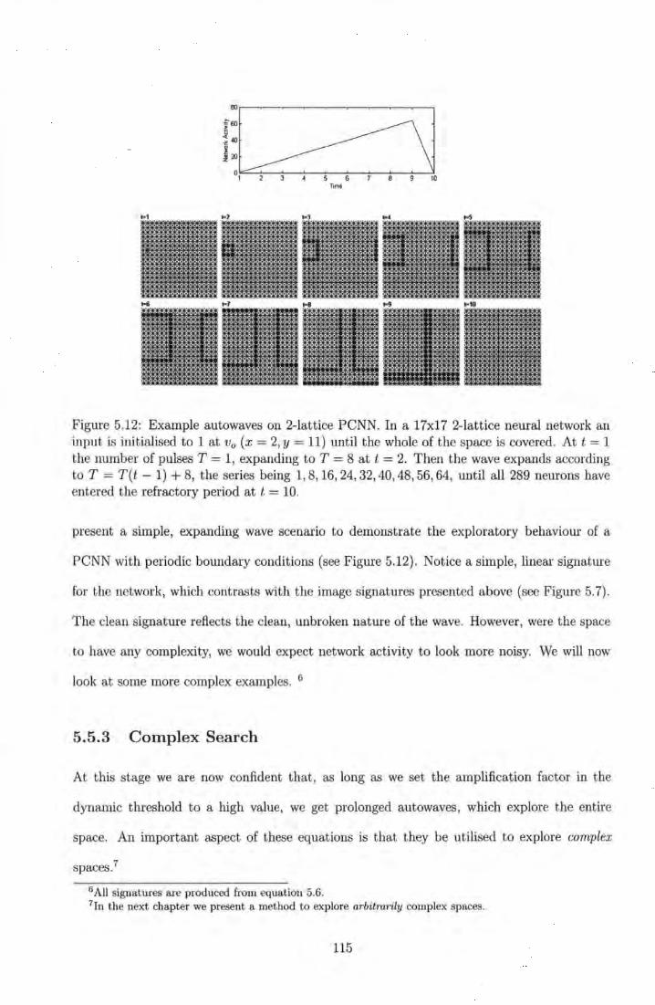
~~~ 1 2 3 4 5 6 7 B 9 10

Timt

Figure 5.12: Example autowaves on 2-lattice PCNN. In a 17x17 2-lattice neural network an input is initialised to 1 at v0 (x = 2, y = 11) until the whole of the space is covered. At t = 1 the number of pulses T = 1, expanding to T = 8 at t = 2. Then the wave expands according to T = T(t - 1) + 8, the series being 1, 8, 16, 24, 32, 40, 48, 56, 64, until all 289 neurons have entered the refractory period at t = 10.

present a simple, expanding wave scenario to demonstrate the exploratory behaviour of a

PCNN with periodic boundary conditions (see Figure 5.12). Notice a simple, linear signature

for the network, which contrasts with the image signatures presented above (see Figure 5.7).

The clean signature reflects the clean, unbroken nature of t he wave. However, were the space

to have any complexity, we would expect network activity to look more noisy. We will now

look at some more complex examples. 6

5.5 .3 Complex Search

At this stage we are now confident that, as long as we set the amplification factor in the

dynamic threshold to a high value, we get prolonged autowaves, which explore the entire

space. An important aspect of these equations is that they be utilised to explore complex

spaces.7

6 All signatures are produced from equation 5.6. 7In the next chapter we present a method to explore arbitrarily complex spaces.

115

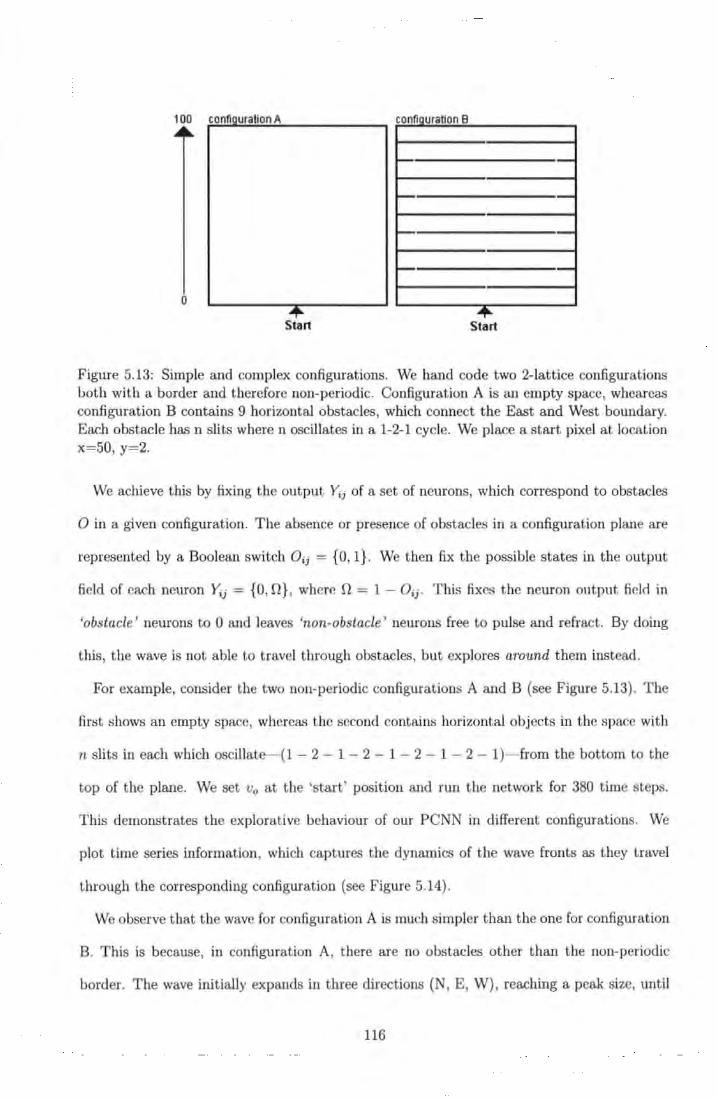
1 00 configuration A

0 +

Start

fi 11 8 con 1gura on

- · ·-

- ·-

·-

·-

+ Start

Figure 5.13: Simple and complex configurations. We hand code two 2-lattice configurations both with a border and therefore non-periodic. Configuration A is an empty space, whcarcas configuration B contains 9 horizontal obstacles, which connect the East and West boundary. Each obstacle has n slits where n oscillates in a 1-2-1 cycle. We place a start pixel at location x=50, y=2.

We achieve this by fixing the output Yii of a set of neurons, which correspond to obstacles

0 in a given configuration. The absence or presence of obstacles in a configuration plane are

represented by a Boolean switch Oii = {0, 1}. We then fix the possible states in the output

field of each neuron Yii = {0, 0}, where 0 = 1 - Oii· This fixes the neuron output field in

'obstacle 1 neurons to 0 and leaves 'non-obstacle 1 neurons free to pulse and refract. By doing

this, the wave is not able to travel through obstacles, but explores around them instead.

For example, consider the two non-periodic configurations A and B (see Figure 5.13). The

first shows an empty space, whereas the second contains horizontal objects in the space with

n slits in each which oscillate-(! - 2- 1 - 2- 1 - 2- 1 - 2- 1)- from the bottom to the

top of the plane. We set v0 at the 'start' position and run the network for 380 time steps.

This demonstrates the explorative behaviour of our PCNN in different configurations. We

plot time series information, which captures the dynamics of the wave fronts as they travel

through the corresponding configuration (see Figure 5.14).

We observe that the wave for configuration A is much simpler than the one for configuration

B. This is because, in configuration A, there are no obstacles other than the non-periodic

border. The wave initially expands in three directions (N, E, W), reaching a peak size, until

116

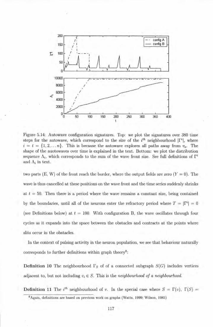
200

I ' -- config A 150 , I - config B

I '

b 100

50

0

10000 / ----

8000 I

6000 /

< 4000

2000

50 100 150 200 250 3(() 350 400

Figure 5.14: Autowave configuration signatures. Top: we plot the signatures over 380 t ime steps for the autowave, which correspond to the size of the ith neighbourhood lfij, where i = t = {1, 2, .. . n}. This is because the autowave explores all paths away from V0 • The shape of the auotowaves over time is explained in the text. Bottom: we plot the distribution sequence Ai, which corresponds to the sum of the wave front size. See full definitions of r i and Ai in text.

two parts (E, W ) of the front reach the border, where the output fields are zero (Y = 0). The

wave is thus cancelled at these positions on the wave front and the time series suddenly shrinks

at t = 50. Then there is a period where the wave remains a constant size, being contained

by the boundaries, until all of the neurons enter the refractory period where T = lfil = 0

(sec Definitions below) at t = 100. With configuration B, the wave oscilla tes through four

cycles as it expands into the space between the obstacles and contracts at the points where

slits occur in the obstacles.

In the context of pulsing activity in the neuron population, we see that behaviour naturally

corresponds to furt her definit ions within graph theory8:

Definition 10 The neighbourhood r s of of a connected subgraph S( G) includes vertices

adjacent to, but not including vi E S . This is the neighbourhood of a neighbourhood.

Definition 11 The ith neighbourhood of v. In the special case where S = r(v), r(S)

8Again, definitions are based on previous work on graphs (Watts, 1999; Wilson, 1985}

117

r(r(v)) = f 2(v) or more generally r(ri-l(v)) = ri(v), the i1h neighbourhood of v, so that

fO(v) = v.

Definition 12 The sequence Ai(v) = 2:{=0 lfi(v)l for 0 ~ j ~ jma:J! is the distribution se

quence for v, where Aim.,(v) = IGI.

Notice that an accumulative value ofT= A;, for a clean, expanding autowave. In this way,

the PCNN described in this section automatically implements a 2-lattice search away from

any given origin.

5.6 Summary

In this chapter we:

• demonstrated how 2-lattice properties determine limits to local search.

• explained the sudden, catastrophic failure of CA dynamics.

• provided a list of appropriate levels of representation for egress and pedestrian dynamics.

• introduced the mechanisms and behaviour of the PCNN, which is compatible with these

levels, and capable of searching beyond limiting localities.

• introduced a more robust PCNN and demonstrated its search capacity within complex

configurations.

• presented PCNN network statistics, in the form of search signatures, and pointed out

how these relate to further Graph Theory definitions.

We have concentrated on inclusive search, local-global linking and obstacle representations.

In the next chapter, we will begin to concentrate more on pedestrian representations and local

dynamics. We will develop techniques derived from autowave search.

118

Chapter 6

Egress Modelling

One of the challenges in building a model is to produce patterns of pedestrian-pedestrian

interaction across all density ranges. Also, a challenge is to produce typical pattern formations

between pedestrian crowds and the environment they occupy. These challenges have not yet

been sufficiently met by models within the pedestrian and evacuation modelling community.

In this chapter we present a set of techniques, which offer an alternative approach to model

specification, in order that such models may be developed.

While implementing a more efficient version of autowave search (sec Section 6.1), we present

the first of these techniques. We look at the limitations of autowave search in multi-agent

scenarios and offer a method designed to overcome these limitations, which is based on the

exploitation of information in search signatures, and the definition of dynamic boundaries

(Section 6.2). We present network-based simulation models to demonstrate the potential

power of our tools (Section 6.3), before briefly summarising the chapter (see Section 6.4).

6.1 Efficient Autowaves

In chapter five, we introduced a search algorithm, based on a Pulse Coupled Neural Network,

and used it for complex spatial exploration. In this section, we present a much more efficient

119

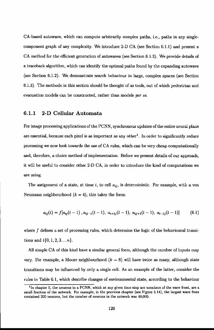
CA-based autowave, which can compute arbitrarily complex paths, i.e., paths in any single-

component graph of any complexity. We introduce 2-D CA (see Section 6.1.1) and present a

CA method for the efficient generation of autowaves (see Section 6.1.2). We provide details of

a traceback algorithm, which can identify the optimal paths found by the expanding autowave

(see Section 6.1.2). We demonstrate search behaviour in large, complex spaces (see Section

6.1.3). The methods in this section should be thought of as tools, out of which pedestrian and

evacuation models can be constructed, rather than models per se.

6.1.1 2-D Cellular Automata

For image processing applications of the PCNN, synchronous updates of the entire neural plane

are essential, because each pixel is as important as any other1. In order to significantly reduce

processing we now look towards the use of CA rules, which can be very cheap computationally

and, therefore, a choice method of implementation. Before we present details of our approach,

it will be useful to consider other 2-D CA, in order to introduce the kind of computations we

are using.

The assignment of a state, at time l, to cell a;j, is deterministic. For example, with a von

Neumann neighbourhood (k = 4), this takes the form:

where f defines a set of processing rules, which determine the logic of the behavioural transi-

tions and l{O, 1, 2, 3 ..... n}.

All simple CA of this kind have a similar general form, although the number of inputs may

vary. For example, a Moore neighbourhood (k = 8) will have twice as many, although state

transitions may be influenced by only a single cell. As an example of the latter, consider the

rules in Table 6.1, which describe changes of environmental state, according to the behaviour

1In chapter 5, the neurons in a PCNN, which at any given time step are members of the wave front, are a small fraction of the network. For example, in the previous chapter (see Figure 5.14), the largest wave front contained 200 neurons, but the number of neurons in the network was 40,000.

120

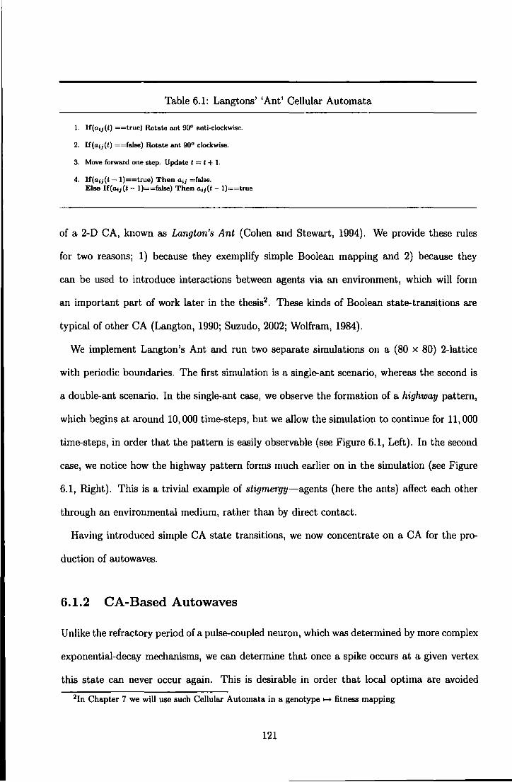
Table 6.1: Langtons' 'Ant' Cellular Automata

1. If(a;j(l) ==true) Rotate ant 90" anti-clockwise.

2. If(a~;(t) ==false) Rotate ant 90° clockwise.

3. Move forward one step. Update t = t + 1.

4. If(a;j(l- !)==true) Then a;j =[alae. Else If(a;j(l- !)==false) Then a;J(I- !)==true

of a 2-D CA, known as Langton's Ant {Cohen and Stewart, 1994). We provide these rules

for two reasons; 1) because they exemplify simple Boolean mapping and 2) because they

can be used to introduce interactions between agents via an environment, which will form

an important part of work later in the thesis2 . These kinds of Boolean state-transitions are

typical of other CA (Langton, 1990; Suzudo, 2002; Wolfram, 1984).

We implement Langton's Ant and run two separate simulations on a (80 x 80) 2-lattice

with periodic boundaries. The first simulation is a single-ant scenario, whereas the second is

a double-ant scenario. In the single-ant case, we observe the formation of a highway pattern,

which begins at around 10, 000 time-steps, but we allow the simulation to continue for 11, 000

time-steps, in order that the pattern is easily observable (see Figure 6.1, Left). In the second

case, we notice how the highway pattern forms much earlier on in the simulation (see Figure

6.1, Right). This is a trivial example of stigmergy-agents {here the ants) affect each other

through an environmental medium, rather than by direct contact.

Having introduced simple CA state transitions, we now concentrate on a CA for the pro-

duction of autowaves.

6.1.2 CA-Based Autowaves

Unlike the refractory period of a pulse-coupled neuron, which was determined by more complex

exponential-decay mechanisl!lS, we can determine that once a spike occurs at a given vertex

this state can never occur again. This is desirable in order that local optima are avoided

2In Chapter 7 we will use such Cellular Automata in a genotype >-+ fitness mapping

121

.................................... .................................... .................................... .................................... .................................... .................................... .................................... .................................... .................................... .................................... .................................... .................................... .................................... .................................... .................................... .................................... .................................... 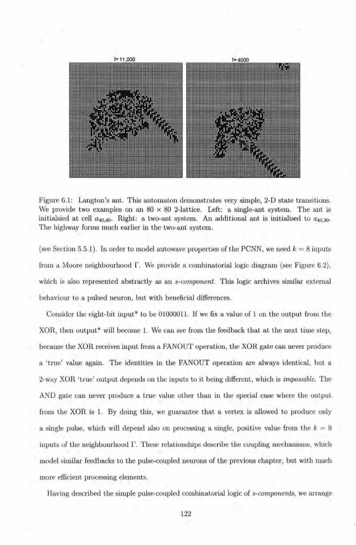iiiiiiiiiii ii i ~ ~i i ~ ~ ~ii ~~ ~i~: i:=: :::

Ill ......................................... ......................................... ......................................... ········································· ......................................... ......................................... ......................................... ......................................... ········································· ......................................... ......................................... ......................................... ......................................... ········································· ......................................... ......................................... ......................................... ......................................... ......................................... .... .............................. . .. ............................... . . . ............................ .. ................................. .............................. .. . . . . ....................... .. ::::::::::::::::::::::::·:::= : ·:.::=-:-:=::::.==·=·= = ::m::::::::m:::::: !g;ggg~g;~~gi=:= =:=;!::·=::;=·:=··:;=::::=.=· =·i·=;HH!m~~imiiign :::::::::::::::::. •• .. :: =::.·.: •· .:=:.:.·r:-·: :·· :·=·:::::m::::m:::::: ::::m::m:::··::: -:·:-.====.····= .:=: :·.:.·: :::: .=·:.:==:::::::::::::::: iiiigg ~i~~ii=: .. : ·= ••• r·~·=: ;;:. :::=::=::·= ·ii· = ·;iii!:: ·. =·::;==ii!gifinn

1~~ ~~m 1 ~~ ~~ ~ j · =:; ~ :l;; 1: l1: ~: :;:l:: :; =; ~: ~ li~~~ ;: ;; ll; ~ ~m~j; l :; ::::~~m~~~~ lllllllll lll!!!~l!~l~~i~@iiiilii~W~jlllli!lllllllllllllllll lllll!lili;i:lll

!llil!llll!lli!lll!lli!!!ill!!lll!!ll!!!l!l!!!!!!!!lll!!lllll!ll!!!ll!ll!!l!!!!

1=4000

.................................................................... .................................................................... .................................................................... .................................................................... .................................................................... .................................................................... .................................................................... ......................... ..................................... . ................... .. ........... ........................ .. .................. ......... ... .......................... . ............ .......... . .. ........................ .. ............... ... ... . ... . ......................... . .............. .. .. ........ ......................... . ............. ..... ... . .... ......................... . .......... . .............. ......................... . ......... . ........ ....... ........................ . .......... . .......... ............................ . ........ ............ ...... ......................... . ......... .. ...... .... .. . ......................... .. ......... . ....................................... .. .......... .. .. ..... .. . .......................... . ........... .. ....... . ........................... . ........... .. ... .. . .. . .......................... . ........... .. ..... . . ............................. . ........... . ..... .. ... .............................. . .......... ······ ... . .. ......................... . .......... ...... .. . . ........................... .. ......... . ... .. ... ................................ .

l!!!i

1

!1iij!iiliJii!J!!!

1

!1:!ii!!:i\iii!!!!:!l!!::IJ!!!I!,!!i!!!ii!;

Figure 6.1: Langton's ant. This automaton demonstrates very simple, 2-D state transitions. We provide two examples on an 80 x 80 2-lattice. Left: a single-ant system. The ant is initialsied at cell a4{),4o. Right: a two-ant system. An additional ant is initialised to a4o,30· The highway forms much earlier in the two-ant system.

(see Section 5.5.1). In order to model autowave properties of the PCNN, we need k = 8 inputs

from a Moore neighbourhood r . We provide a combinatorial logic diagram (see Figure 6.2) ,

which is also represented abstractly as an s-component. This logic archives similar external

behaviour to a pulsed neuron, but with beneficial differences.

Consider the eight-bit input* to be 01000011. If we fix a value of 1 on the output from the

XOR, then output* will become 1. We can see from the feedback that at the next time step,

because the XOR receives input from a FAN OUT operation, the XOR gate can never produce

a 'true' value again. The identities in the FANOUT operation are always identical , but a

2-way XOR 'true' output depends on the inputs to it being different, which is impossible. The

AND gate can never produce a true value other than in the special case where the output

from the XOR is 1. By doing this, we guarantee that a vertex is allowed to produce only

a single pulse, which will depend also on processing a single, positive value from the k = 8

inputs of the neighbourhood r. These relationships describe the coupling mechanisms, which

model similar feedbacks to the pulse-coupled neurons of the previous chapter, but with much

more efficient processing elements.

Having described the simple pulse-coupled combinatorial logic of s-components, we arrange

122

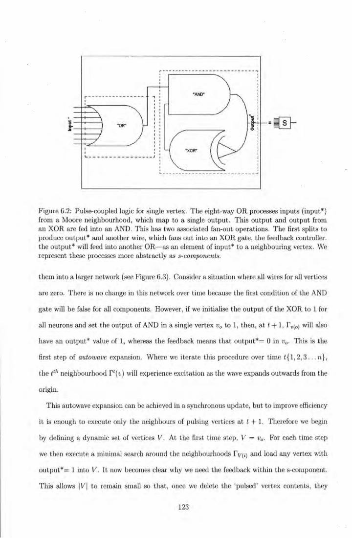
r---------------- ,

. -H---\

f--+-t---i I I

"'R"

~----------- -- ---

I

r- ·-------------------------~

"At¥)"

=@-

"X OR"

0

---------------------------~

Figure 6.2: Pulse-coupled logic for single vertex. The eight-way OR processes inputs (input*) from a Moore neighbourhood, which map to a single output. This output and output from an XOR are fed into an AND. This has two associated fan-out operations. The first splits to produce output* and another wire, which fans out into an XOR gate, the feedback controller. the output* will feed into another OR-as an element of input* to a neighbouring vertex. We represent these processes more abstractly as s-components.

them into a larger network (see Figure 6.3). Consider a situation where all wires for all vertices

are zero. There is no change in this network over time because the first condition of the AND

gate will be false for all components. However, if we initialise the output of the XOR to 1 for

all neurons and set the output of AND in a single vertex v0 to 1, then, at t + 1, r v(o) will also

have an output* value of 1, whereas the feedback means that output*= 0 in v0 • This is the

first step of autowave expansion. Where we iterate this procedure over t ime t{1, 2, 3 . . . n},

the tth neighbourhood rt( v) will experience excitation as the wave expands outwards from the

origin.

This autowave expansion can be achieved in a synchronous update, but to improve efficiency

it is enough to execute only the neighbours of pulsing vertices at t + 1. Therefore we begin

by defining a dynamic set of vertices V. At the first time step, V = v0 . For each time step

we then execute a minimal search around the neighbourhoods fv(i) and load any vertex with

output*= 1 into V. It now becomes clear why we need the feedback within the s-component.

This allows lVI to remain small so that, once we delete the 'pulsed' vertex contents, they

123

=

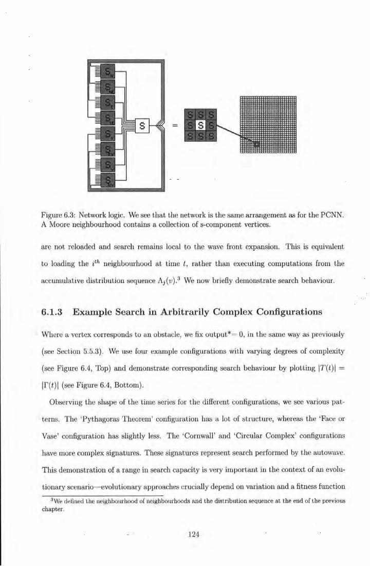
Figure 6.3: Network logic. We see that the network is t he same arrangement as for the PCNN. A Moore neighbourhood contains a collection of s-component vertices.

are not reloaded and search remains local to the wave front expansion. This is equivalent

to loading the ith neighbourhood at time t, rather t han executing computations from the

accumulative distribut ion sequence Aj(v) .3 We now briefly demonstrate search behaviour.

6.1.3 Example Search in Arbitrarily Complex Configurations

Where a vertex corresponds to an obstacle, we fix output*= 0, in the same way as previously

(see Section 5.5.3) . We use four example configurations with varying degrees of complexity

(see Figure 6.4, Top) and demonstrate corresponding search behaviour by plotting IT(t)l =

lr(t)l (see Figure 6.4, Bottom).

Observing the shape of the time series for the different configurations, we see various pat-

terns. The 'Pythagoras Theorem' configuration has a lot of structure, whereas the 'Face or

Vase' configuration has slightly less. T he 'Cornwall' and 'Circular Complex' configurations

have more complex signatures. These signatures represent search performed by the autowave.

This demonstration of a range in search capacity is very important in the context of an evolu-

t ionary scenario-evolutionary approaches crucially depend on variation and a fitness function

3We defined the neighbourhood of neighbourhoods and the distribution sequence at the end of the previous chapter.

124

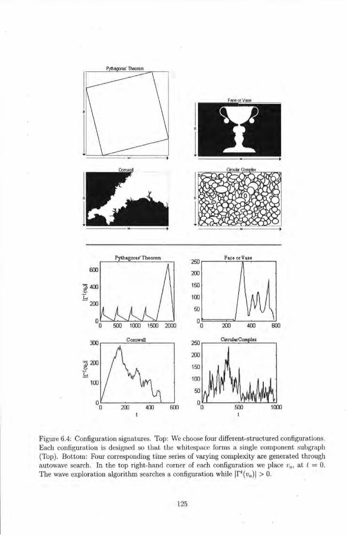
Pythagoras' Theorem 250

600 200

~400 150

r.... 100 200

50

0 0 500 Hlll 1500 2000

0 0 200 400 600

300 Comwall 250

CircularCom lex

200

~200 ..., 150 1

Figure 6.4: Configuration signatures. Top: We choose four different-structured configurations. Each configuration is designed so that the whitespace forms a single component subgraph (Top) . Bottom: Fom corresponding time series of varying complexity are generated through autowave search. In the top right-hand corner of each configuration we place v0 , at l = 0. The wave exploration algorithm searches a configuration while lft(vo) l > 0.

125

has to cope with the variation available from within a given population (see Chapter 7).

From the presentation of the algorithm in this section, it should be clear that any single

component graph is explored within the constraints of a computational environment. We now

present the nature of the trace-back search, which occurs when a wave travels from V0 and

'hits' a destination vertex vd.

6.1.4 'fraceback Algorithm

The aforementioned autowave advances away from V0 at each time-step (~t = 1). As the

wave advances, we record on each pulsed vertex a value of the pulse time t. When the halting

condition is met (vd(output•) = 1), pulsed vertices represent a time-dependant field. For trace

back search, we start at the destination vertex vd and search rvd. We search for vertices with

tv(i) = tv(d) - ~t, i.e., vertices which pulsed in the previous time step. We then load these

vertices to V. We repeat this procedure for fv(il• until V0 is reached. Vertices v;i E V define a

connected subgraph S(G) from v 0 to vd. It follows from this description that because ~t = 1,

then vd contains a valueD, which is the diameter of S(G).

Definition 13 The Graph diameter is the step distance between two maximally seperated

vertices. This is equivalent to the time between v0 and vd, where ~t = 1.

We illustrate the concept of graph diameter with an example configuration in the shape

of a smiley face (see Figure 6.5). The figure shows a graph G with vertices subject to fixed

output*= 0, represented in dark grey. We set v0 to the coordinate of the right eye of the

face and vd to a coordinate above the face. near the northern boundary of G. We show the

subgraph S(G), which has a diameter of 37.

6.1.5 Summary

In this section we:

126

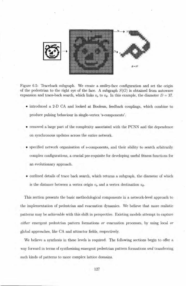
Figure 6.5: Traceback subgraph. We create a smiley-face configuration and set the origin of the pedestrian to the right eye of the face. A subgraph S( G) is obtained from autowave expansion and trace-back search, which links v0 to vd. In this example, the diameter D = 37.

• introduced a 2-D CA and looked at Boolean, feedback couplings, which combine to

produce pulsing behaviour in single-vertex 's-components'.

• removed a large part of the complexity associated with the PCNN and the dependence

on synchronous updates across the entire network.

• specified network organisation of s-components, and their ability to search arbitrarily

complex configurations, a crucial pre-requisite for developing useful fitness functions for

an evolutionary approach.

• outlined details of t race back search, which returns a subgraph, the diameter of which

is the distance between a vertex origin V0 and a vertex destination vd.

This section presents the basic methodological components in a network-level approach to

the implementation of pedestrian and evacuation dynamics. We believe that more realistic

patterns may be achievable with this shift in perspective. Existing models attempt to capture

either emergent pedestrian pattern formations or evacuation processes, by using local or

global approaches, like CA and attractor fields, respectively.

We believe a synthesis in these levels is required. The following sections begin to offer a

way forward in terms of synthesising emergent pedestrian pattern formations and t ransferring

such kinds of patterns to more complex lattice domains.

127

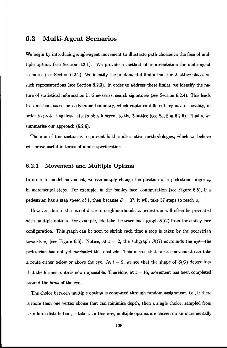
6.2 Multi-Agent Scenarios

We begin by introducing single-agent movement to illustrate path choices in the face of mul

tiple optima (see Section 6.2.1). We provide a method of representation for multi-agent

scenarios (see Section 6.2.2). We identify the fundamental limits that the 2-lattice places on

such representations (see Section 6.2.3). In order to address these limits, we identify the na

ture of statistical information in time-series, search signatures (see Section 6.2.4). This leads

to a method based on a dynamic boundary, which captures different regimes of locality, in

order to protect against catastrophes inherent to the 2-lattice (see Section 6.2.5). Finally, we

summarise our approach (6.2.6).

The aim of this section is to present further alternative methodologies, which we believe

will prove useful in terms of model specification.

6.2.1 Movement and Multiple Optima

In order to model movement, we can simply change the position of a pedestrian origin V 0

in incremental steps. For example, in the 'smiley face' configuration (see Figure 6.5), if a

pedestrian has a step speed of 1, then because D = 37, it will take 37 steps to reach Vd·

However, due to the use of discrete neighbourhoods, a pedestrian will often be presented

with multiple optima. For example, lets take the trace-back graph S(G) from the smiley face

configuration. This graph can be seen to shrink each time a step is taken by the pedestrian

towards vd (see Figure 6.6). Notice, at t = 2, the subgraph S(G) surrounds the eye-the

pedestrian has not yet navigated this obstacle. This means that future movement can take

a route either below or above the eye. At t = 9, we see that the shape of S( G) determines

that the former route is now impossible. Therefore, at t = 16, movement has been completed

around the brow of the eye.

The choice between multiple optima is computed through random assignment, i.e., if there

is more than one vertex choice that can minimise depth, then a single choice, sampled from

a uniform distribution, is taken. In this way, multiple optima are chosen on an incrementally

128

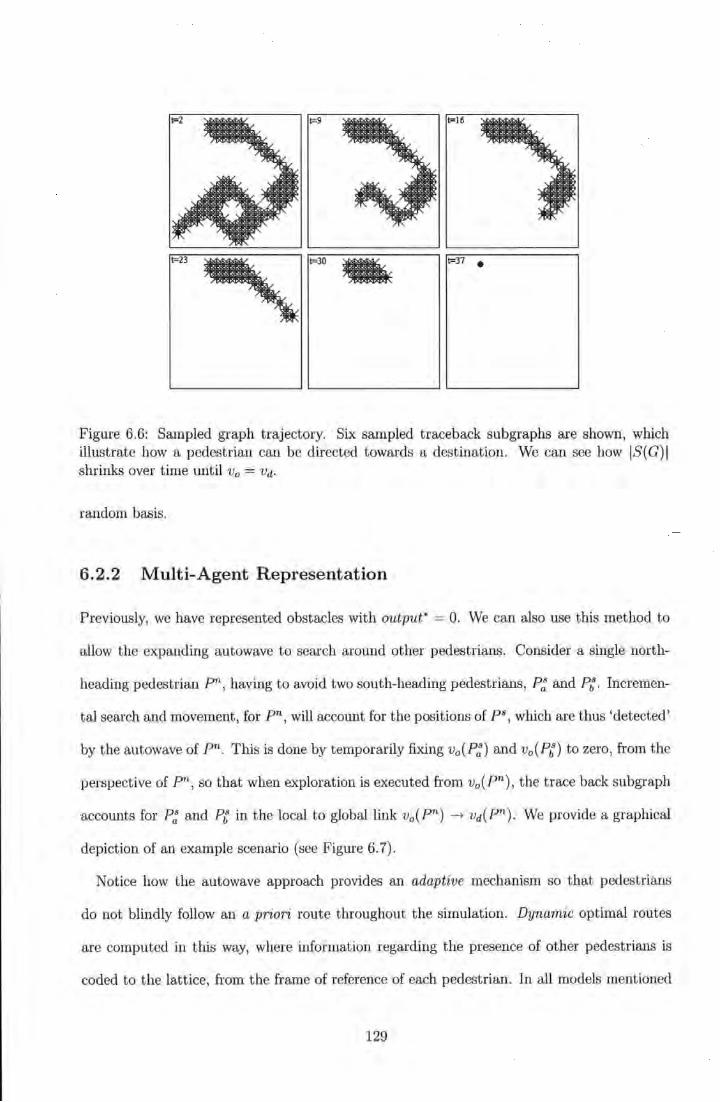
t=23

~FJO t=37 •

Figure 6.6: Sampled graph trajectory. Six sampled traceback subgraphs are shown, which illustrate how a pedestrian can be directed towards a destination. We can see how IS(G)I shrinks over time until V0 = vd.

random basis.

6.2.2 Multi-Agent Representation

Previously, we have represented obstacles with output* = 0. We can also use this method to

allow the expanding autowave to search around other pedestrians. Consider a single north-

heading pedestrian pn, having to avoid two south-heading pedestrians, P~ and Pt . Incremen-

tal search and movement, for pn , will account for the positions of P8, which are thus 'detected '

by the autowave of pn. This is done by temporarily fixing va(P~) and v0 (Pt) to zero, from the

perspective of P'\ so that when exploration is executed from va(Pn), the trace back subgraph

accounts for P~ and Pt in the local to global link v0 (Pn) ---+ vd(Pn). We provide a graphical

depiction of an example scenario (see Figure 6.7) .

Notice how the autowave approach provides an adaptive mechanism so that pedestrians

do not blindly follow an a priori route throughout the simulation. Dynamic optimal routes

are computed in t his way, where information regarding the presence of other pedestrians is

coded to the lattice, from the frame of reference of each pedestrian. In all models mentioned

129

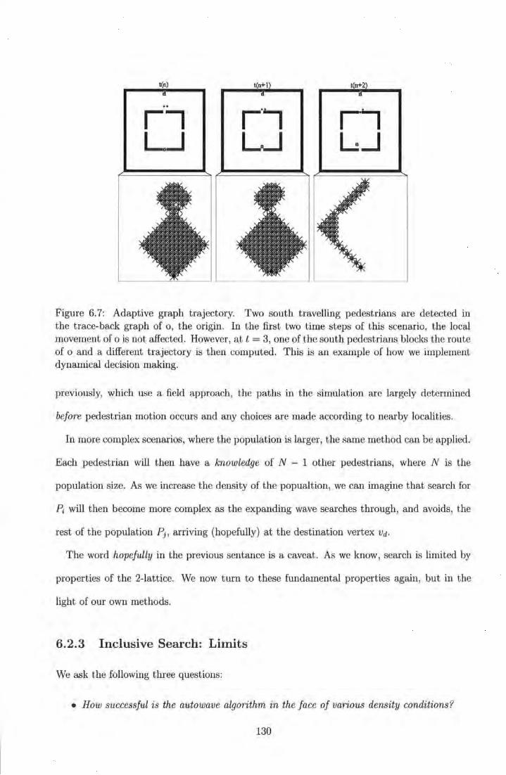
n+l) t(n+2)

rl l..:_l

Figure 6. 7: Adaptive graph trajectory. Two south travelling pedestrians are detected in the trace-back graph of o, t he origin. In the first two time steps of this scenario, the local movement of o is not affected. However, at t = 3, one of the south pedestrians blocks the route of o and a different trajectory is then computed. This is an example of how we implement dynamical decision making.

previously, which use a field approach, the paths in the simulation are largely determined

before pedestrian motion occurs and any choices are made according to nearby localities.

In more complex scenarios, where the population is larger, the same method can be applied.

Each pedestrian will then have a knowledge of N - 1 other pedestrians, where N is the

population size. As we increase the density of the popualtion, we can imagine that search for

~ will then become more complex as the expanding wave searches through, and avoids, the

rest of the population Pj, arriving (hopefully) at the destination vertex Vd.

The word hopefully in the previous sentance is a caveat. As we know, search is limited by

properties of the 2-lattice. We now turn to these fundamental properties again, but in the

light of our own methods.

6.2.3 Inclusive Search: Limits

We ask the following three questions:

• How successful is the autowave algorithm in the face of various density conditions?

130

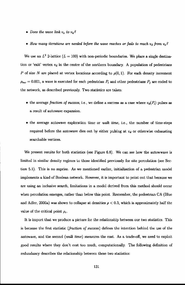
• Does the wave link V 0 to Vd?

• How many itemtions are needed before the wave reaches or fails to reach vd from V0 ?

We use an L2 2-lattice (L = 100) with non-periodic boundaries. We place a single destina

tion or 'exit' vertex vd in the centre of the northern boundary. A population of pedestrians

P of size N are placed at vertex locations according to p(O, 1). For each density increment

Pine = 0.001, a wave is executed for each pedestrian P; and other pedestrians Pi are coded to

the network, as described previously. Two statistics are taken:

• the average fraction of success, i.e., we define a success as a case where vd(P;) pulses as

a result of autowave expansion.

• the average autowave exploration time or walk time, i.e., the number of time-steps

required before the autowave dies out by either pulsing at vd or otherwise exhausting

searchable vertices.

We present results for both statistics (see Figure 6.8). We can see how the autowwave is

limited in similar density regimes to those identified previously for site percolation (see Sec

tion 5.1). This is no suprise. As we mentioned earlier, initialisation of a pedestrian model

implements a kind of Boolean network. However, it is important to point out that because we

are using an inclusive search, limitations in a model derived from this method should occur

when percolation emerges, rather than below this point. Remember, the pedestrian CA (Blue

and Adler, 2000a) was shown to collapse at densities p < 0.3, which is approximately half the

value of the critical point Pc·

It is import that we produce a picture for the relationship between our two statistics. This

is because the first statistic (fraction of success) defines the intention behind the use of the

autowave, and the second (walk time) measures the cost. As a trade-off, we need to exploit

good results where they don't cost too much, computationally. The following definition of

redundancy describes the relationship between these two statistics:

131

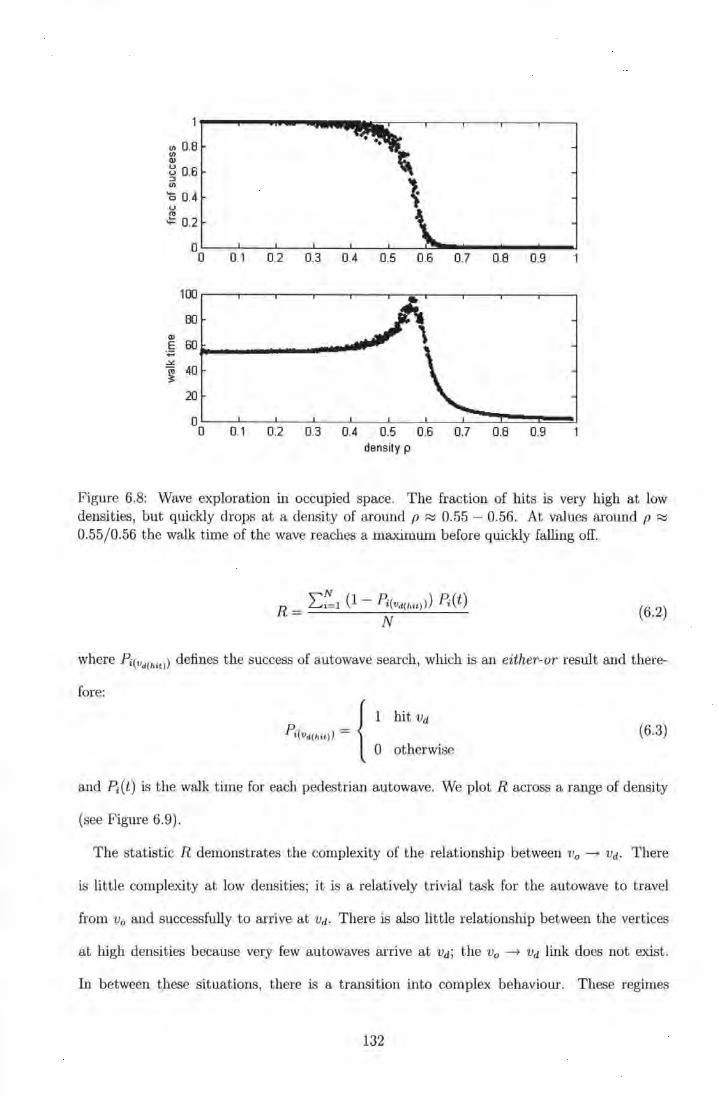
(/) 0.8 (/) Q)

t: 0.6 :::3

l (/)

'0 0.4 u RI

.::: 0.2

0 0 0.1 0.2 0.3 0.4 0.5 0.6 0.7 0.8 0.9

100

80 Q)

E 60 ·.;::::; .:Y!.

l 40

20

0 0 0.1 0.2 0.3 0.4 0.5 0.6 0.7 0.8 0.9

density p

Figure 6.8: Wave exploration in occupied space. The fraction of hits is very high at low densities, but quickly drops at a density of around p ~ 0.55 - 0.56. At values around p ~

0.55/0.56 the walk time of the wave reaches a maximum before quickly falling off.

R = 2::1 (1- pi(vd(ha))) ~(t) N

(6.2)

where Pi(vd(ha)) defines t he success of autowave search, which is an either-or result and there-

fore:

{

1 hit Vd

p i (vd(hit)l = 0 otherwise

(6.3)

and ~(t) is the walk t ime for each pedestrian autowave. We plot R across a range of density

(see Figure 6.9).

The statistic R demonstrates the complexity of the relationship between v 0 -t vd . There

is little complexity at low densities; it is a relatively trivial task for the autowave to travel

from v 0 and successfully to arrive at vd. There is also little relationship between the vertices

at high densities because very few autowaves arrive at vd; the V0 -t vd link does not exist.

In between these situations, there is a transition into complex behaviour. These regimes

132

00.---.---.----.---.---.----.---.----.---.---.

70

60

50

er 40

30

20

10

0.1 0.2 0.3 0.4 0.5 0.6 0.7 0.8 0.9 densit y p

Figure 6.9: Redundancy in wave exploration. Wave redundancy R is a measure of the success and walk time of an autowave. Redundancy peaks at a value p ~ 5.9, which is in close agreement with results of critical points in 2-lattices (Stauffer and Aharony, 1992).

demonstrate the possible limitations of using the autowave approach. There are therefore

practical consequences of this critical range-if there are few 'hits ', then few pedestrians can

produce a trace-back path, which as we have seen is the backbone of our adaptive search

method.

6.2.4 Use of Time Series Signatures

Previously, we demonstrated the importance of S(G). We defined the diameter D(S), which

is equivalent to the amount of time spent searching from v0 to vd (see Section 6.1.4) . Notice

that the graph diameter D = Pi(t) (equation 6.1). Therefore, for a given pedestrian~. where

the regime is complex between Vo; and Vet,, we observe a high value for D( S)i.

We present examples of S( G) for two different values of density p = 0.59 and p = 0.4

(see Figure 6.10) . For p = 0.59, S(G) is thin, which means that the graph is brittle; if another

pedestrian Pi were to occupy V0 i E S(G) , then the link v0 --. vd would probably break. For

133

p = 0.4, S(G) is fatter, which means that the graph is more robust; if another pedestrian Pi

were to occupy V 0 J E S(G), this would not break the link V0 --+ vd.

This poses a problem: how do we tackle the brittleness of autowave search in increasingly

high density regimes? The solution to this problem needs to be simple. Any complex algorithm

would be outside of computational limitations. We need to try and exploit information in the

autowave signature, which as we have demonstrated previously, represents the complexity of

search. More specifically, we ask is there information we can use in the time signature of

autowave search to control the nature of the search pedestrians execute? What we are looking

for is an indicator that the autowave front will die before reaching vd.

An obvious question to ask about the autowave search is if the wave front shrinks to a value

of 1, then what is the probability of quick failure thereafter? Firstly, we will identify whether

or not the autowave from V0 to vd contains a value of 1. If so, we refer to this as a 'one-type'

signature. Secondly, we need to know how much time elapses before a one-type signature fails.

These two conditions represent a lower limit, and the simplest case, where an heuristic may

be introduced into the search method in order to improve robustness in and above critical

regimes.

We identify one-type signatures and present the fraction of failed searches that contain a

value of 1 in the search signature (see Figure 6.11). We can see that the fraction of one

type signatures quickly increases within the critical ranges identified above. However, an

important property is that, above this range, the fall-off of one-type signatures is relatively

smooth. The majority of pedestrians still produce one-type signatures in a fairly large density

range p ~ (0.6, 0.88). This means that, although search is failing in terms of the v0 --+ vd link,

it is likely that a large amount of potentially useful search is being undertaken above Pc·

It will also be useful to know particular properties of this search. We would not expect,

given a wave front thats shrinks to 1, much more progress of this front. In order to get a

statistical description, we present interval histograms, which represent the critical range of

density p = (0.51- 0.6) (see Figure 6.12). Each histogram shows the conditional probability,

134

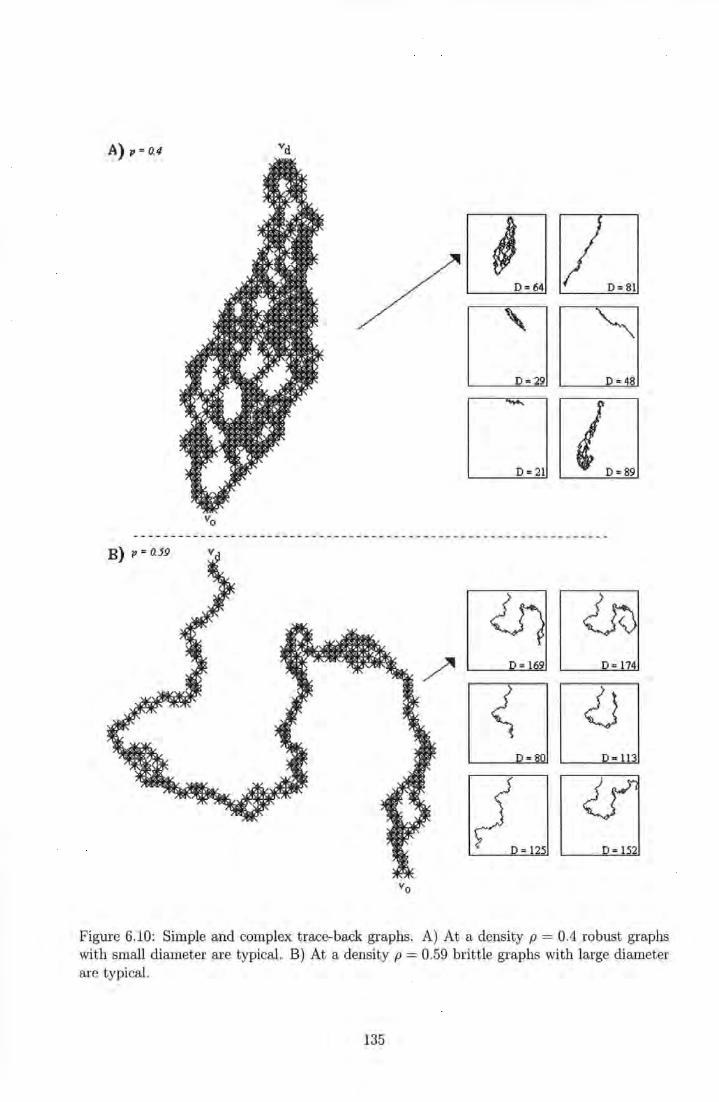
A),= 0.4

B) , = o.59

Figure 6.10: Simple and complex trace-back graphs. A) At a density p = 0.4 robust graphs with small diameter are typical. B) At a density p = 0.59 brittle graphs with large diameter are typical.

135

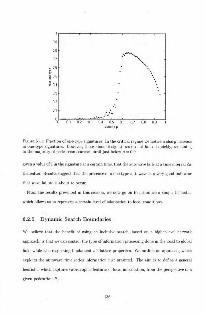
0.9

0.8

0.7

~ 0.6 a.. ~ ~ 0.5 0

~ .!:: 0.4

0.3

0.2

0.1

. . . • . . ...

........... . ... •• •• •• ..

• • • • • • • . • •

• •

• •• . . .. ,.,. 004-..... ----~~~~~--~---L---L--~--~--~

0.1 0.2 0.3 0.4 0.5 0.6 0.7 0.8 0.9 density p

Figure 6.11: Fraction of one-type signatures. In the critical regime we notice a sharp increase in one-type signatures. However, these kinds of signatures do not fall off quickly, remaining in the majority of pedestrian searches until just below p = 0.9.

given a value of 1 in the signature at a certain time, that the autowave fails at a time interval ~t

thereafter. Results suggest that t he presence of a one-type autowave is a very good indicator

that wave failure is about to occur.

From the results presented in this section, we now go on to introduce a simple heuristic,

which allows us to represent a certain level of adaptation to local conditions.

6.2.5 Dynamic Search Boundaries

We believe that the benefit of using an inclusive search, based on a higher-level network

approach, is that we can control the type of information processing done in the local to global

link, while also respecting fundamental 2-lattice properties. We outline an approach, which

exploits the autowave time series information just presnted. T he aim is to define a general

heuristic, which captures catastrophic features of local information, from the perspective of a

given pedestrian Pi.

136

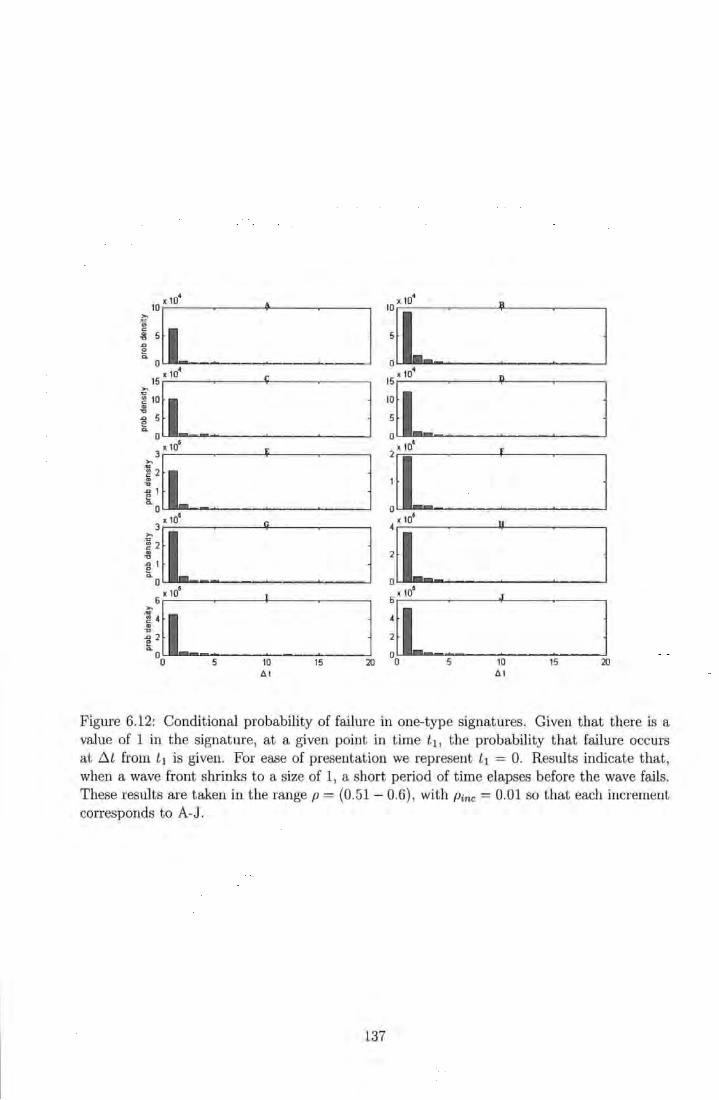
( [ ·~ ~ : : J': [ [ __ ' : : l I :~ [ ~~ -~ : : l :~ [ ~~- : : : l l~[l~ -: : ' l Ji_ : : : l t:[f -~ : : l :ii __ ' : : l ([1~-~ : . l ;ri~-~ : : l

0 5 10 15 20 0 5 10 15 20 Lit .0.1

Figure 6.12: Conditional probability of failure in one-type signatures. Given that there is a value of 1 in the signature, at a given point in time t1 , the probability that failure occurs at !:lt from l 1 is given. For ease of presentation we represent t1 = 0. Results indicate that, when a wave front shrinks to a size of 1, a short period of time elapses before the wave fails. These results are taken in the range p = (0.51 - 0.6) , with Pine = 0.01 so that each increment corresponds to A-J.

137

We use time series information to determine likely points of search failure, which, as we

have seen, relate to times in autowave search when the wave front shrinks to a value of 1. We

then identify the point of failure VJ,· We then define the Manhattan radius rm from v0 , to VJ;

and construct a boundary B; = {v E G: v = rm}.

We present two examples of this method (see Figure 6.13). We show the times series search

of both examples. In example A, failure occurs at the second step (t = 16) after the wave

front shrinks to 1 (t = 14). In example B, failure occurs at the fourth step (t = 6) after

the wave front shrinks to 1 (t = 2). Underneath each time series, we present corresponding

geometrical information. The subgraph Sr( G) = { v E G : v < rm} corresponds to a robust

region of search, i.e., where the front has not yet shrunk to the value of 1. The subgraph

Sb( G) = { v E G : v > rm} corresponds to a brittle region. We identify v0 , ( +), walkable

vertices (grey), which the wave front can move through, and post type-one search vertices

(x). The first occurrence of an x-vertex is used to define the radius rm.

For each pedestrian P;, a boundary B; can be used to define which inputs are set to the

network. If we do not account for other pedestrians Pi located Vo; E Sb( G);, then the autowave

will be able to propagate to vd. The trace back graph S(G); would not contain information

on all pedestrians between V0 -+ vd. However, S(G); would still indicate a good move to make

in the face of local information, defined inside the boundary, i.e., v E Sr.

In this way, locality is defined dynamically and with respect to the nature of information

between the origin of any given pedestrian and the destination of that pedestrian. This

method represents a trade-off between gaining useful information Sr(G) and gaining too much

information Sb(G). We believe this approach is valid because even in the case where there is

high probability of broken V0 -+ vd linkage, there remains a large amount of potentially useful

search.

We demonstrate how, at densities above the critical range, search can percolate outside v0

to fairly large areas (see Figure 6.14). The spaces show distributions of post type-one search

vertices, but represented differently ( x = •). In these simulations, we set v0 to the centre

138

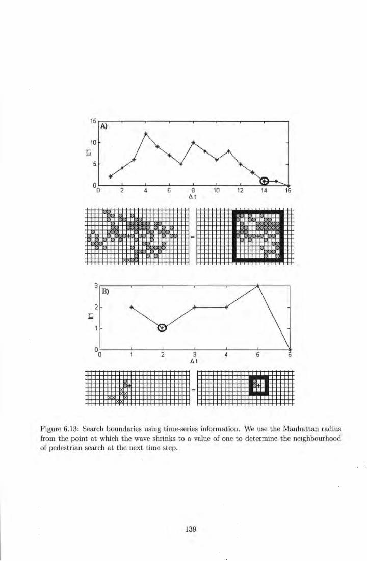
15 A)

10

b

5

10 12 14 16 .O.t

··=--·

111111111111111111111= 11111111111111~111111 Figure 6.13: Search boundaries using time-series information. We use the Manhattan radius from the point at which the wave shrinks to a value of one to determine the neighbourhood of pedestrian search at the next time step.

139

• ••

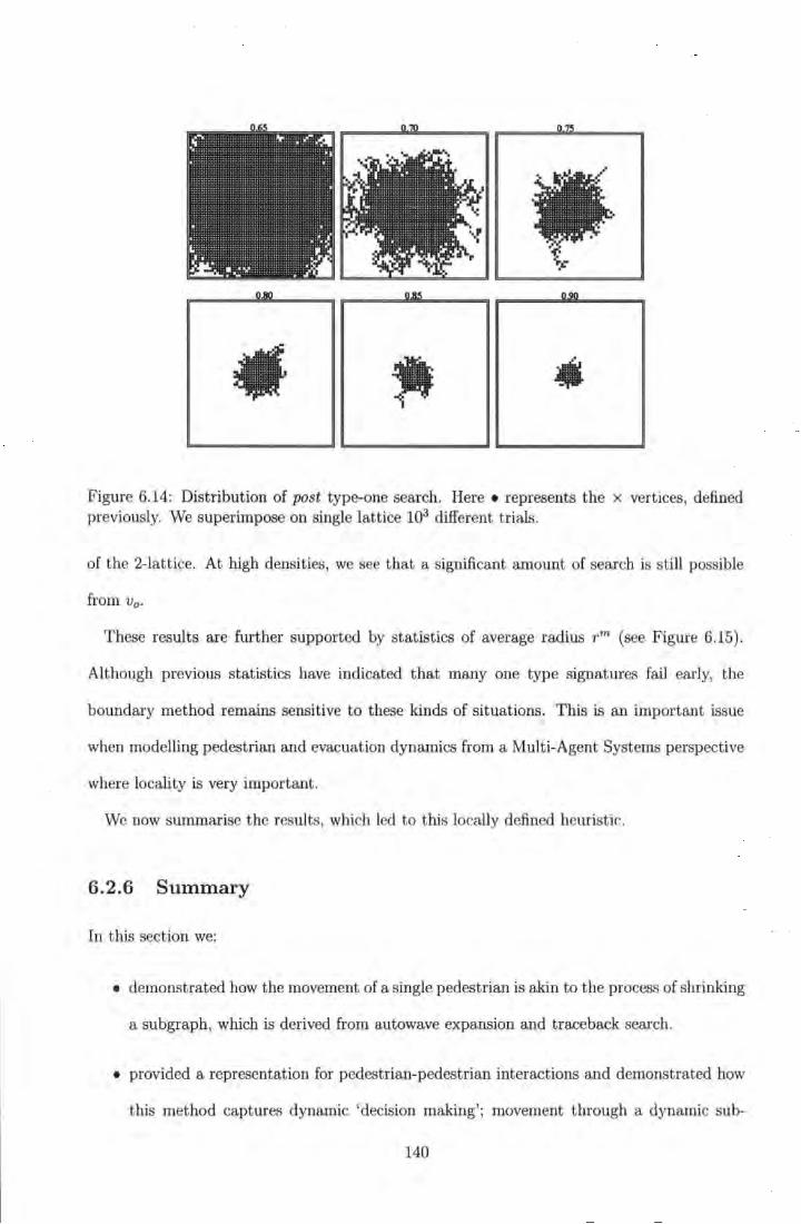
Figure 6.14: Distribution of post type-one search. Here • represents the x vertices, defined previously. We superimpose on single lattice 103 different t rials.

of the 2-lattice. At high densities, we see that a significant amount of search is still possible

from V 0 .

These results are further supported by statistics of average radius rm (see Figure 6.15).

Although previous statistics have indicated that many one type signatures fail early, the

boundary method remains sensitive to these kinds of situations. This is an important issue

when modelling pedestrian and evacuation dynamics from a Multi-Agent Systems perspective

where locality is very important.

We now summarise the results, which led to this locally defined heuristic.

6.2.6 Summary

In this section we:

• demonstrated how the movement of a single pedestrian is akin to the process of shrinking

a subgraph, which is derived from autowave expansion and tra.ceba.ck search.

• provided a representation for pedestrian-pedestrian interactions and demonstrated how

this method captures dynamic 'decision making'; movement through a dynamic sub-

140

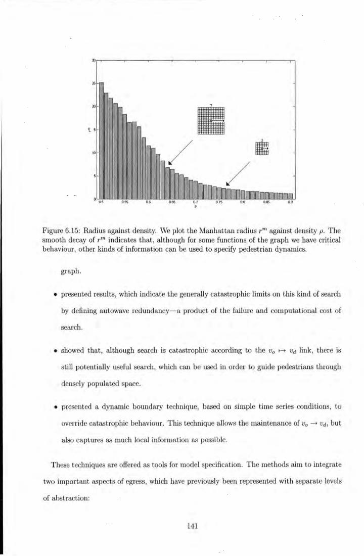
~or-----.----.-----.-----.-----.-----.-----.-----~

25

lD

• t 5

10 / 0.5 0.55 06 0.66

Figure 6.15: Radius against density. We plot the Manhattan radius rm against density p. The smooth decay of rm indicates that, although for some functions of t he graph we have critical behaviour, other kinds of information can be used to specify pedestrian dynamics.

graph.

• presented results, which indicate the generally catastrophic limits on this kind of search

by defining autowave redundancy- a product of the failure and computational cost of

search.

• showed that, although search is catastrophic according to the V0 1-4 vd link, there is

still potentially useful search, which can be used in order to guide pedestrians through

densely populated space.

• presented a dynamic boundary technique, based on simple time series conditions, to

override catastrophic behaviour. This technique allows the maintenance of V0 ---+ vd, but

also captures as much local information as possible.

These techniques are offered as tools for model specification. The methods aim to integrate

two important aspects of egress, which have previously been represented with separate levels

of abstraction:

141

1. local dynamics of pedestrian-pedestrian interactions (e.g., cellular automata).

2. longer-range goal of egress (e.g., attractor fields).

We now test the usefulness of our methods by presenting two computational models.

6.3 Simulation Models: Pedestrian Pattern Formation

We present an alternative model of lane formation behaviour (see Section 6.3.1). We also

demonstrate how our techniques are portable by simulating a more complex egress scenario,

but with only minor model adjustments (see Section 6.3.2).

One of the major motivations for the techniques developed in this thesis rest upon the

belief that there are fundamental geometrical patterns formed in crowds and that crowd-flow

statistics are determined by these patterns. It is therefore insufficient to present statisti

cal results of, e.g., crowd-flow v density without looking also at the geometrical patterns of

pedestrian-pedestrian interaction in a model.

6.3.1 Lane-Formation

One of the most frequently observed phenomenon in real crowds of pedestrians is the devel

opment of lane formations (Helbing et al., 2000; Blue and Adler, 2000a; Still, 2000). This is

generally regarded as an important emergent property of groups of pedestrians where optimi

sation of forward movement is thought to be motivating factor.

In order to model this behaviour, it is important to provide each pedestrian with knowledge

of the positions of surrounding pedestrians. We have previously outlined an approach for

representing the positions of other agents (e.g., see Section 6.2.2). In other models, directional

movement is achieved by, for example, introducing a relaxation term to a vector (Helbing

et al., 2000) or by labelling each pedestrian and creating rules around these labels (Blue and

Adler, 2000a). As ours is a discrete model, we also label our pedestrians and then use this label

to determine which pedestrians are accounted for in the network. The assumptions behind

142

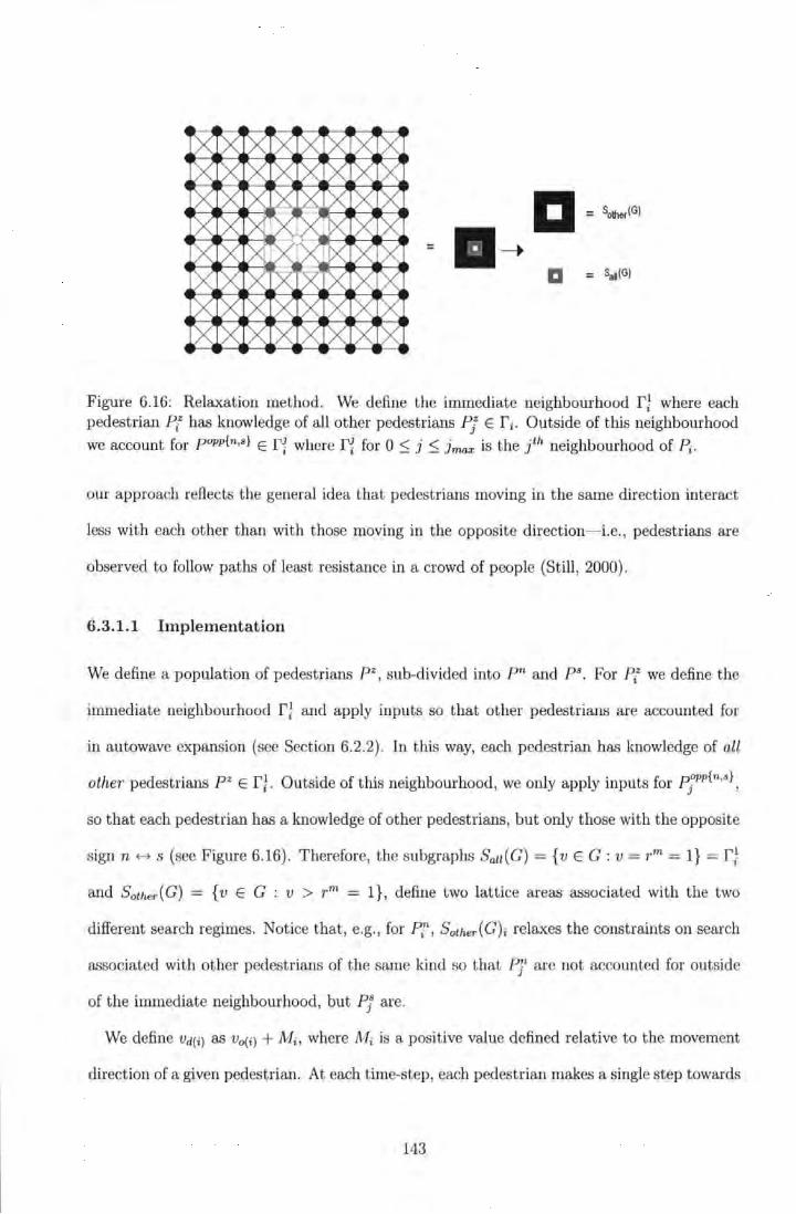
a = 5other(G)

= ____.

a = saa(G)

Figure 6.16: Relaxation method. We define the immediate neighbourhood rf where each pedestrian P{ has knowledge of all other pedestrians Pj E ri· Outside of this neighbourhood we account for popp{n,s} E fj where f~ for 0 < J. < J. is the J·th neighbourhood of P..

t t - - max t

our approach reflects the general idea that pedestrians moving in the same direction interact

less with each other than with those moving in the opposite direction- i.e. , pedestrians are

observed to follow paths of least resistance in a crowd of people (Still, 2000) .

6.3.1.1 Implementation

We define a population of pedestrians p z, sub-divided into pn and ps. For P{ we define the

immediate neighbourhood r; and apply inputs so that other pedestrians are accounted for

in autowave expansion (see Section 6.2.2) . In this way, each pedestrian has knowledge of all

other pedestrians p z E f!. Outside of this neighbourhood, we only apply inputs for P jopp{n,s},

so that each pedestrian has a knowledge of other pedestrians, but only those with the opposite

sign n t-t s (see Figure 6.16) . Therefore, the subgraphs Sau(G) = {v E G: V= 1' m = 1} = n and Sother(G) = {v E G : v > rm = 1}, define two lattice areas associated with the two

different search regimes. Notice that, e.g., for Pi, Bother ( G)i relaxes the constraints on search

associated with other pedestrians of the same kind so that PJ1 are not accounted for outside

of the immediate neighbourhood, but PJ are.

We define Vd(i) as Vo(i) + Mi , where M i is a positive value defined relative to the movement

direction of a given pedestrian. At each time-step, each pedestrian makes a single step towards

143

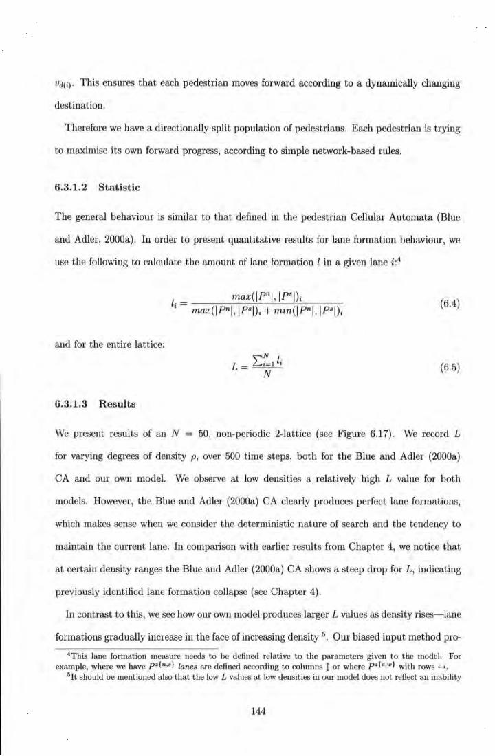
vd(i)· This ensures that each pedestrian moves forward according to a dynamically changing

destination.

Therefore we have a directionally split population of pedestrians. Each pedestrian is trying

to maximise its own forward progress, according to simple network-based rules.

6.3.1.2 Statistic

The general behaviour is similar to t hat defined in the pedestrian Cellular Automata (Blue

and Adler, 2000a) . In order to present quantitative results for lane formation behaviour, we

use the following to calculate the amount of lane formation l in a given lane i:4

li = max( ipnl.iP•i)i max(ipni, IP•i)i + min(ipni, IP•i)i (6.4)

and for the entire lattice:

(6.5)

6.3.1.3 Results

We present results of an N = 50, non-periodic 2-lattice (see Figure 6.17). We record L

for varying degrees of density p, over 500 time steps, both for the Blue and Adler (2000a)

CA and our own model. We observe at low densities a relatively high L value for both

models. However, the Blue and Adler (2000a) CA clearly produces perfect lane formations,

which makes sense when we consider the deterministic nature of search and the tendency to

maintain the current lane. In comparison with earlier results from Chapter 4, we notice that

at certain density ranges the Blue and Adler (2000a) CA shows a steep drop for L, indicating

previously identified lane formation collapse (see Chapter 4).

In contrast to this, we see how our own model produces larger L values as density rises-lane

formations gradually increase in the face of increasing density 5 . Our biased input method pro-

4This lane formation measure needs to be defined relative to t he parameters given to the model. For example, where we have pz{n,s} lanes are defined according to columns 1 or where p z{e,w} with rows ......

5It should be mentioned also that the low L values at low densities in our model does not reflect an inability

144

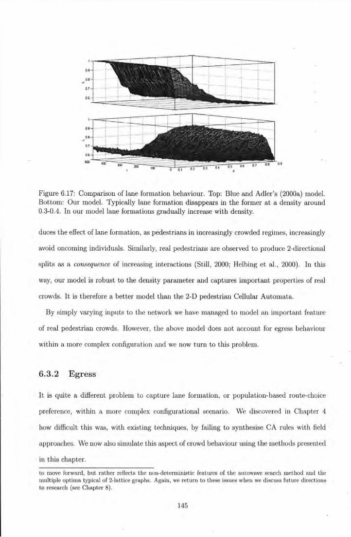
Figure 6.17: Comparison of lane formation behaviour. Top: Blue and Adler's (2000a) model. Bottom: Our model. Typically lane formation disappears in the former at a density around 0.3-0.4. In our model lane formations gradually increase with density.

duces the effect of lane formation, as pedestrians in increasingly crowded regimes, increasingly

avoid oncoming individuals. Similarly, real pedestrians are observed to produce 2-directional

splits as a consequence of increasing interactions (Still, 2000; Helbing et al., 2000) . In this

way, our model is robust to the density parameter and captmes important properties of real

crowds. It is therefore a better model than the 2-D pedestrian Cellular Automata.

By simply varying inputs to the network we have managed to model an important feature

of real pedestrian crowds. However, the above model does not accow1t for egress behaviour

within a more complex configuration and we now turn to this problem.

6.3.2 Egress

It is quite a different problem to capture lane formation, or population-based route-choice

preference, within a more complex configurational scenario. We discovered in Chapter 4

how difficult this was, with existing techniques, by failing to synthesise CA rules with field

approaches. We now also simulate this aspect of crowd behaviour using the methods presented

in this chapter.

to move forward, but rather reflects the non-deterministic features of the autowave search method and the multiple optima typical of 2-lattice graphs. Again, we return to these issues when we discuss future directions to research (see Chapter 8}.

145

Figure 6.18: Two-door, two-exit configuration. We set t he destination of each pedestrian population to different exit vertices. We initialise both populations randomly to the white space. Grey areas represent obstacles or walls.

6.3.2.1 Implementation

The implementation is very similar to that of the previous model, where we use the same

relaxation method, but port it to a more complex 2-lattice scenario. We define two sets

of pedestrians, pe and pw, whose destination vertices correspond to two fixed destination

vertices, vf and v~, respectively (see Figure 6.18) . We initialise the pedestrians randomly

within the white space of the configuration. Each pedestrian pz then moves towards its

designated exit vertex, avoiding other pedestrians, in the same way as described in the more

simple model above.

6.3.2.2 Results

We demonstrate the behaviour produced for different time steps (see Figure 6.19). Pedestrians

with the same destination vertex are attracted to the same doors. The attraction-to-same-

door behaviour is an effect produced by the autowave method-'door preference' reflects the

ability of autowave search to exploit and accumulate early fluctuations from random pedestrian

initialisation. This accumulation is encouraged by the relaxation method used.

6.3.3 Summary

This simulation section engages with other discrete models of pedestrian and evacuation dy-

namics. In the literature we find no other methods, which can model both navigation/evacuation

processes and higher-level pedestrian pattern formations. We believe this direction is an im-

portant challenge for the pedestrian and evacuation dynamics community. In terms of produc-

146

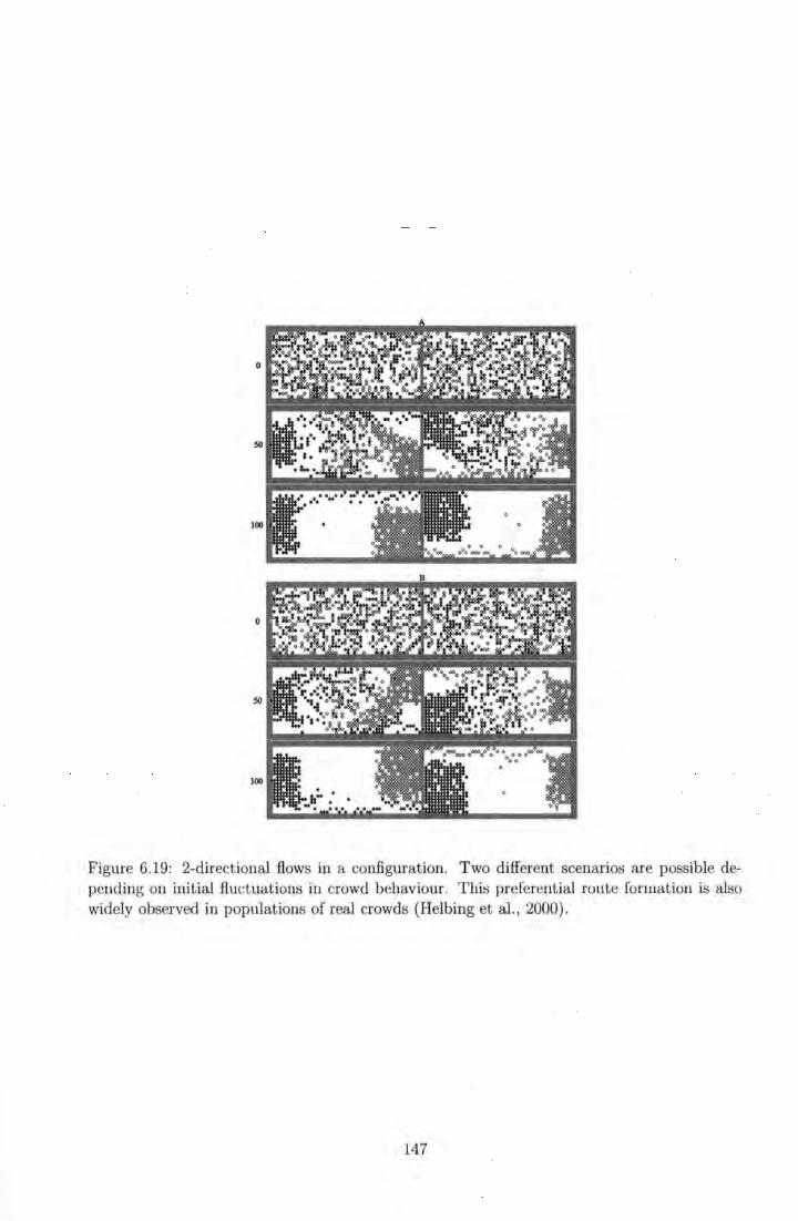
Figure 6.19: 2-directional flows in a configuration. Two different scenarios are possible depending on initial fluctuations in crowd behaviour. This preferent ial route formation is also widely observed in populations of real crowds (Helbing et al. , 2000).

147

ing evacuation behaviour, while also allowing for the emergence of important developmental

patterns, the simulations presented here represent preliminary work and indicate positive

results obtainable through the use of simple network-level methods.

We believe this is an important shift in empha.sis away from models, which either model

pedestrian-pedestrian interactions (and ignore higher-level behaviour) or rely on more global,

fixed field representations for escape (and ignore more local interactions).

6.4 Summary

In this chapter we:

• developed a number of techniques to specify pedestrian and evacuation models ba.sed

on:

- efficient autowave search.

- trace-back search.

- representations for obstacle avoidance.

- path-choice methods in the face of multiple optima.

- properties of search robustness.

- a dynamic boundary to protect local dynamics.

• demonstrated the potential power of these techniques by specifying two simulation mod

els, which define preliminary attempts to integrate two previously separate levels of

representation.

This point in the thesis defines an end to work on the development of egress models. For the

rest of the thesis we take our model at face value. We will discuss some of its general limitations

in our conclusions (see Chapter 8), but firstly we see how these techniques, or improvements

to them, might be used in the context of an evolutionary approach to architectural design.

148

Chapter 7

Evolutionary Architecture

The aim of this chapter is to demonstrate the utility of techniques developed in chapters 5

and 6 in the context of Evolutionary Design. Before this is possible we need to address the

specific problem of how to represent valid, single-component graphs inside a genetic code.

Previously in the thesis, configurations have been hand-coded. In the context of evolutionary

design, however, an automatic development of valid designs is needed. As a starting point,

we therefore look at two nature-inspired models of self-organising architecture (see Section

7.1). We then present the kind of architectural spaces we seek to develop (see Section 7.2).

Based on ideas from the nature-inspired models, we present a self-organising algorithm for the

development of 2-D architectures (see Section 7.3).

We then concentrate on artificial evolution. We outline the Simple Genetic Algorithm and

discuss evolutionary dynamics (see Section 7.4). We present two evolutionary approaches. In

the first we exploit our self-organising algorithm by genetically encoding certain parameters

(see Section 7.5). This approach is concerned with the evolution of generative architecture.

The second approach is a simpler application of constrained evolution (see Section 7.6). Again,

we summarise at the end of the chapter (see Section 7.7).

149

7.1 Nature-Inspired Growth

In this section, we review two nature-inspired models of generative architecture. We look

at nest building (see Section 7.1.1) and crystal formation (see Section 7.1.2), which have

social insects and atoms in motion as respective agents of growth. Both models enable us to

introduce the kind of methods that we think are appropriate for the automated generation of

architectural forms. We identify specific features of these models, which bear on choices made

in the design of our own developmental algorithm, presented later (see Section 7.2).

7 .1.1 Social Insects

In nature, wasps are able to construct a range of architectural forms on the basis of very

simple rules, which are triggered by environmental stimuli. For example, the first act of nest

construction begins with a deposit of material on an initial site. The nest then accumulates

and expands from this site until nest building is complete. In this way, the nest grows from

a small seed into a complex architecture. Potentially, there is a combinatorial explosion of

possible forms during growth. As Bonabeau et al. (1999) state: "The number of possible

sites where a new cell can be added increase.~ significantly as the construction proceeds". In

this scenario, it is easy to imagine a disorganisation of the building process as the number

of possible interactions increases, but it appears that the building structure, while enabling

growth, at the same time constrains and channels it- " ... the building decisions seem to be made

locally on the basis of percei11ed configurations in a way that po.~sibly con..~trains the building

dynamics"(p 212). In short, the potential of diffusion to run away aimlessly is checked by the

self-organising properties of the rules.

In the work by Bonabeau et al. {1999) virtual wasps build nest architectures. The origi

nal stimulus, akin to an initial deposit, consists of a single brick vertex vb, embedded within

a 3-lattice graph G. Each wasp-like agent has a sensory capacity defined by a 3-D Moore

neighbourhood, consisting of 26 vertices. This sensory environment defines a stimulating con

figuration on which micro-rules operate. The latter trigger local brick-depositing behaviours

150

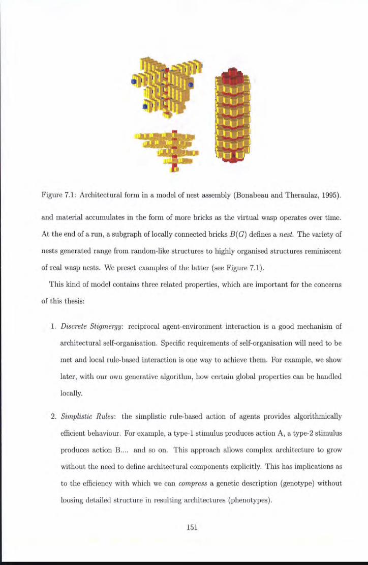
Figure 7.1: Architectural form in a model of nest assembly (Bonabeau and Theraulaz, 1995) .

and material accumulates in the form of more bricks as the virtual wasp operates over time.

At the end of a run, a subgraph of locally connected bricks B( G) defines a nest. The variety of

nests generated range from random-like structures to highly organised structures reminiscent

of real wasp nests. We preset examples of the latter (see Figure 7.1).

This kind of model contains three related properties, which are important for the concerns

of this thesis:

1. Discrete Stigmergy: reciprocal agent-environment interaction is a good mechanism of

architectural self-organisation. Specific requirements of self-organisation will need to be

met and local rule-based interaction is one way to achieve them. For example, we show

later, with our own generative algorithm, how certain global properties can be handled

locally.

2. Simplistic Rules: the simplistic rule-based action of agents provides algorithmically

efficient behaviour. For example, a type-1 stimulus produces action A, a type-2 stimulus

produces action B... . and so on. This approach allows complex architecture to grow

without the need to define architectural components explicitly. This has implications as

to the efficiency with which we can compress a genetic description (genotype) without

loosing detailed structure in resulting architectures (phenotypes).

151

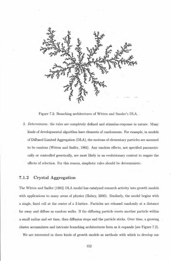
Figure 7.2: Branching architectures of Witten and Sander's DLA.

3. Determinism: the rules are completely defined and stimulus-response in nature. Many

kinds of developmental algorithm have elements of randomness. For example, in models

of Diffused Limited Aggregation (DLA) , the motions of elementary particles are assumed

to be random (Witten and Sadler, 1983). Any random effects, not specified parametri

cally or controlled genetically, are most likely in an evolutionary context to negate the

effects of selection. For this reason, simplistic rules should be deterministic.

7 .1. 2 Crystal Aggregation

The Witten and Sadler (1983) DLA model has catalysed research activity into growth models

with applications to many areas of physics (Halsey, 2000). Similarly, the model begins with

a single, fixed cell at the centre of a 2-lattice. Particles are released randomly at a distance

far away and diffuse as random walks. If the diffusing particle meets another particle within

a small radius and set t ime, t hen diffusion stops and the particle sticks. Over t ime, a growing

cluster accumulates and intricate branching architectures form as it expands (see Figure 7.2).

We are interested in these kinds of growth models as methods with which to develop our

152

own generative architectures. Of more specific interest is a parameter-controlled version of

DLA where various kinds of morphologies can be tuned into the dynamics of growth (D'Souza

and Margolus, 1999). In this model, details of particle interactious are based on less abstract

natural processes-exchange of heat and energy conseroation-whereas particles in the former

DLA are added to a space artificially.

The state of a single vertex in a 2-lattice is defined by a set of 7 bits N;(i, t):

• one crystal Nc(i, t) particle.

• two gas NJ(i, t) particles.

• two heat NZ(i, t) particles.

• one random variable ~9(i, t).

• one random variable ~h(i, t).

where"'= {1, 2}. There are two steps in the dynamics:

1. Diffusion, which consists of two subprocedures:

(a) Mixing. This proceeds according to the following rules:

Nl = (1- ~;)Nl + ~;Nf

where i = g or i = h-mixing only occurs between the same kind of particle.

(7.1)

(b) Transport. A parameter k defines a distance on the lattice and each of the particles

takes on the corresponding value of the k1h vertex away from the current site

at alternative time steps i + k, where i = i at l{2, 4, 6, 8 ... n} and i = ii at

t{1, 3, 7, 9 ... n}. This completes the diffusion dynamics. The diffusion constant k

can take on different values kh and k9 so that the subsystems can be controlled

separately.

153

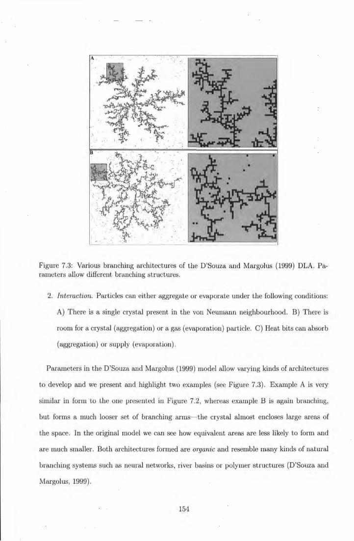
Figure 7.3: Various branching architectures of the D'Souza and Margolus (1999) DLA. Parameters allow different branching structures.

2. Interaction. Particles can either aggregate or evaporate under the following conditions:

A) T here is a single crystal present in the von Neumann neighbourhood. B) There is

room for a crystal (aggregation) or a gas (evaporation) particle. C) Heat bits can absorb

(aggregation) or supply (evaporation).

Parameters in the D'Souza and Margolus (1999) model allow varying kinds of architectures

to develop and we present and highlight two examples (see Figure 7.3). Example A is very

similar in form to the one presented in Figure 7.2, whereas example B is again branching,

but forms a much looser set of branching arms- the crystal almost encloses large areas of

the space. In the original model we can see how equivalent areas are less likely to form and

are much smaller. Both architectures formed are organic and resemble many kinds of natural

branching systems such as neural networks, river basins or polymer structures (D'Souza and

Margolus, 1999).

154

For the concerns of this thesis, there are 2 desirable properties of this model:

• Single component graphs: The model forms a single component crystal by aggregating

at local sites. For the concerns of this thesis, as previously mentioned, it is essential that

we produce single component spaces. To qualify this, what is essential, for us, is not

particularly that the crystal, but specifically that the space in which the crystal grows,

be single-component. Unlike other kinds of architecture (neural), where recurrent con

nections might be important (Wheeler, 1996), cyclic connections in the 2-lattice crystal

would fracture regions of space. A rule of aggregation (rule A) specifies that a crystal

can be aggregated if, and only if, a single crystal is already within the neighbourhood.

This rule prevents the formation of cyclic growth in crystals. This property is important

for autowave search, which requires connection from v0 and vd.

• Parameter-Based: The model is parameter-based and allows some variety in architec

tural form to develop. In an evolutionary context it is essential that a variety of archi

tectures can develop from a single model because evolution requires variation in order

to make selection meaningful. We will return to this issue in the next section.

However, there are also two undesirable properties:

• Organic structure: The architectures that develop are very organic in nature and very

much at odds with the qualitative nature of architectural representation used for built

human forms (Hillier, 1996).

• Updating: The implementation of this model depends on a synchronous update of the

entire lattice. In a population-based approach we need to reduce any unnecessary com

putation time.

It would be beneficial if we could create an architectural generator, which created more

realistic forms, but also did so without the need for this kind of global update.

155

7.1.3 Summary

In order to evolve architectural configurations we believe it is necessary to design a genemtive

algorithm. As a precursor to doing so we have:

• Identified some potentially important methods by reviewing two approaches to architec

tural form generation.

• Listed some specific algorithmic mechanisms.

• Identified desirable and undesirable properties.

We now briefly consider architectural spaces, before we offer our own generative algorithm,

which builds on some of the ideas presented in this section.

7.2 Architectural Spaces

In chapter 3, we introduced the Theory of Space Syntax (Hillier, 1996). We present two

example architectural representations from this work (see Figure 7.4). Consider breaking

these configurations into a number of components. For example, we can decompose 'A' into

two main components; 1) a 1-dimensional corridor with seven vertices and 2) a nine-vertex

square room. These kinds of structures are very easy to hand-design, but, as we have seen,

this ease may not be so obvious from the point of view of automatic architectural generation.

The examples presented previously have shown overly organic structures, which are a very

different form to the examples presented here.

However, we belive it is a generative approach, which we need to apply. Architectural

decompositions have been used in some methods of form generation using Genetic Algo

rithms, where components, represented as grammatical rules are combined into various forms

(Rosenman, 1996). These forms are made with a human-in-the-loop process, where Architects

evaluate forms at each step in an evolutionary run. However, spaces that result from this pro

cess do not maintain any internal structure, but only define a boundary form where all of the

156

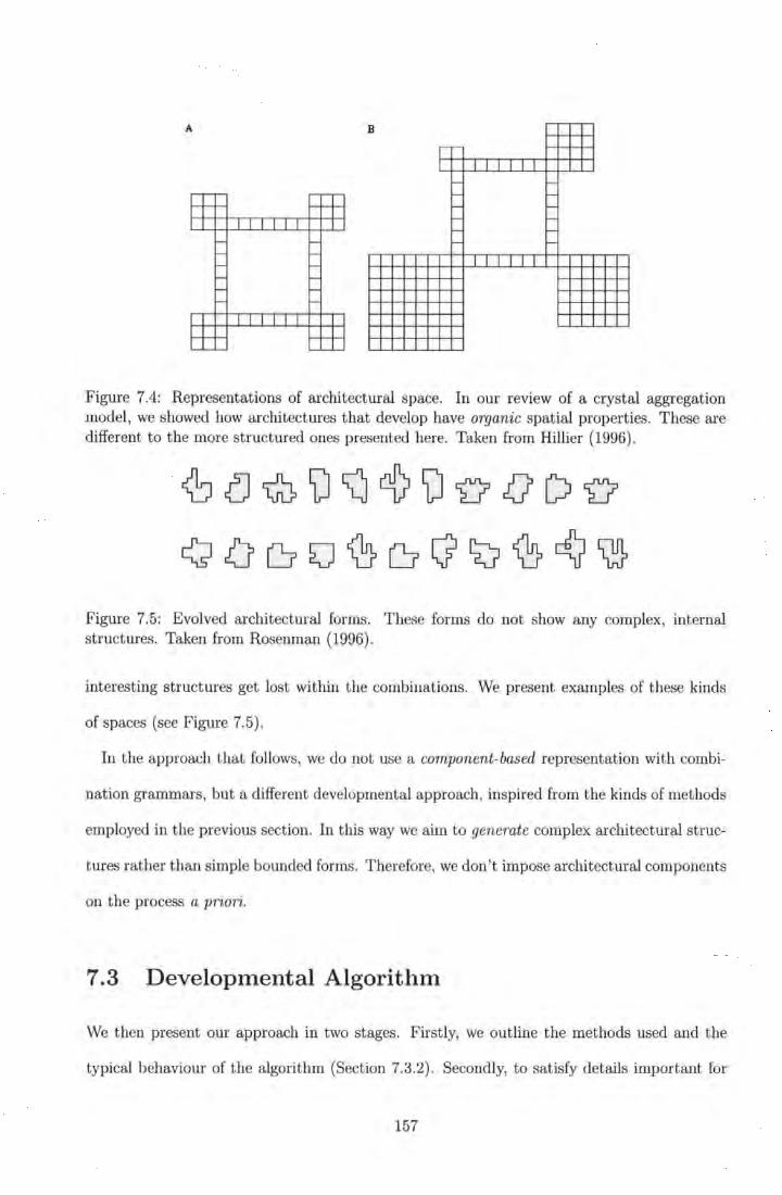
A B

I' L l_lllll

t- -t- -t- -t- -t- -t- -

j_ll_j ll

Figure 7.4: Representations of architectural space. In our review of a crystal aggregation model, we showed how architectures that develop have organic spatial properties. These are different to the more structured ones presented here. Taken from Hillier {1996).

Figure 7.5: Evolved architectural forms. These forms do not show any complex, internal structures. Taken from Rosenman {1996).

interesting structures get lost within the combinations. We present examples of these kinds

of spaces (see Figure 7.5).

In the approach that follows, we do not use a component-based representation with combi-

nation grammars, but a different developmental approach, inspired from the kinds of methods

employed in t he previous section. In this way we aim to generate complex architectural struc-

tures rather than simple bounded forms. Therefore, we don't impose architectural components

on the process a priori.

7.3 Developmental Algorithm

We then present our approach in two stages. Firstly, we outline the methods used and the

typical behaviour of the algorithm (Section 7.3.2). Secondly, to satisfy details important for

157

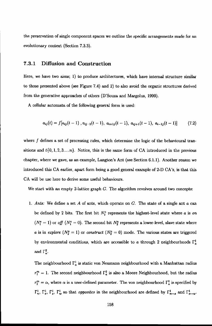
the preservation of single component spaces we outline the specific arrangements made for an

evolutionary context (Section 7.3.3).

7.3.1 Diffusion and Construction

Here, we have two aims; 1) to produce architectures, which have internal structure similar

to those presented above (see Figure 7.4) and 2) to also avoid the organic structures derived

from the generative approaches of others (D'Souza and Margolus, 1999).

A cellular automata of the following general form is used:

Clij(t) = f[a;j(t- 1), a;;-I(t- 1), lli+Ij(t- 1), Clij+I(t- 1), Cli-Ij(t- 1)] {7.2)

where f defines a set of processing rules, which determine the logic of the behavioural tran

sitions and t{O, 1, 2, 3 ..... n}. Notice, this is the same form of CA introduced in the previous

chapter, where we gave, as an example, Langton's Ant {see Section 6.1.1). Another reason we

introduced this CA earlier, apart form being a good general example of 2-D CA's, is that this

CA will be use here to derive some useful behaviours.

We start with an empty 2-lattice graph G. The algorithm revolves around two concepts:

1. Ants: We define a set A of ants, which operate on G. The state of a single ant a can

be defined by 2 bits. The first bit Nj represents the highest-level state where a is on

(Nj = 1) or off (Nj = 0). The second bit N~ represents a lower-level, slave state where

a is in explore (N~ = 1) or construct (N~ = 0) mode. The various states are triggered

by environmental conditions, which are accessible to a through 2 neighbourhoods f!

and r~.

The neighbourhood f! is static von Neumann neighbourhood with a Manhattan radius

rj = 1. The second neighbourhood r~ is also a Moore Neighbourhood, but the radius

r2 =et, where et is a user-defined parameter. The von neighbourhood f! is specified by

r~, r!, r!, r~ so that opposites in the neighbourhood are defined by r~-· and r!-w·

158

Table 7.1: Modified Version of Langton's Ant

1. lf(v.(t) = true) Rotate ant 90° anti-clockwise.

2. lf(v.(t) = false) Rotate ant 90° clockwise.

3. Move forward two steps. Increment t = t + .O.t.

4. lf(v0 (1- I)= true) Then v0 (t- I)= false. Else lf(v0 (1- 1) = false) Then v0 (t- l)=true.

5. lf(r~(N' = 1)) Then enter Construct Mode.

Table 7.2: Construct Mode

I. IF(f~(N' = 1)) AND IF(f!(N' = 0)) ant =off

2. IF(f!(N' = 1)) drop seed on Vo and move forward one step

In the event that a seed is found in elements n, e, s or w of f 1, then the ant direction

d = s, w, n, e, respectively.

2. Seeds: We define a set of seed vertices S E G. Each seed is controlled by a single bit

N", which allows a seed to be present (N" = 1) of absent (N" = 0).

While an ant is on (Nf = 1) and in an explore (N!J = 1) mode, it follows rules derived from

Langton's ant. This phase of behaviour can be thought of as a general diffusion phase. In this

phase a conditional rule, which can trigger a change of state from N!J = 1 to N!J = 0, allows

the ant to enter a construct phase. (see Table 7.1). The algorithm, therefore, consists of a set

of ants A(i, t), where the rules in the exploration and build mode determine the interchange

of i (i or Y'J. The set of seeds S grows according to the construct mode (see Table 7.2). Each

ant diffuses according to these rules and enters a build mode depending on the stimulation

condition in f 1 or halts depending on the stimulation condition in f 2.

We define G to be a 2-lattice (N = 100). We place A9 randomly on vii• where j = i =

{2k+ 1: k E Z} and 0 < k <N. We place sh randomly on Vtm. where l =m= {2k: k E Z}.

Therefore ants can only be initialised to odd locations in the lattice, whereas seeds can only

159

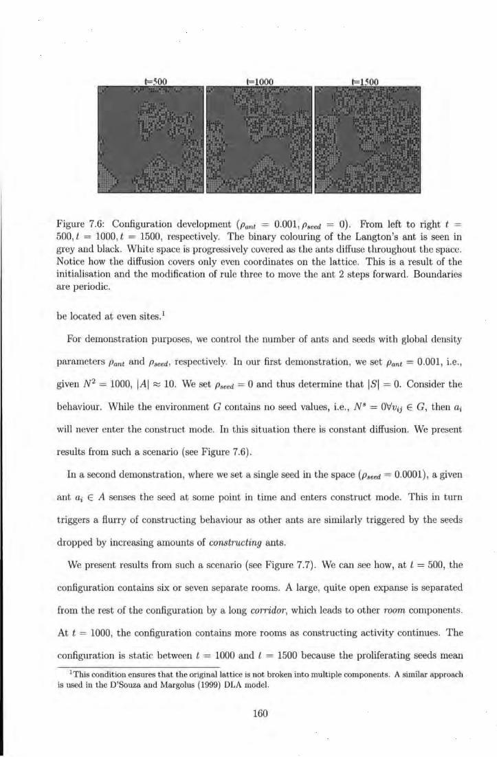
Figure 7.6: Configuration development (Pant = 0.001, Pseed = 0). From left to right t = 500, t = 1000, t = 1500, respectively. The binary colouring of the Langton's ant is seen in grey and black. White space is progressively covered as the ants diffuse throughout the space. Notice how the diffusion covers only even coordinates on the lattice. This is a result of the initialisation and the modification of rule three to move the ant 2 steps forward. Boundaries are periodic.

be located at even sites.1

For demonstration purposes, we control the number of ants and seeds with global density

parameters Pant and Pseed , respectively. In our first demonstration, we set Pant = 0.001, i.e.,

given N2 = 1000, IAI ~ 10. We set Pseed = 0 and thus determine that ISI = 0. Consider the

behaviour. While the environment G contains no seed values, i.e., N 8 = OVvii E G, then ai

will never enter t he construct mode. In this situation there is constant diffusion. We present

results from such a scenario (see Figure 7.6).

In a second demonstration, where we set a single seed in the space (Pseed = 0.0001), a given

ant ai E A senses the seed at some point in time and enters construct mode. This in turn

triggers a flurry of constructing behaviour as other ants are similarly triggered by the seeds

dropped by increasing amounts of constructing ants.

We present results from such a scenario (see Figure 7.7). We can see how, at L = 500, the

configuration contains six or seven separate rooms. A large, quite open expanse is separated

from the rest of the configuration by a long corridor, which leads to other room components.

At t = 1000, the configuration contains more rooms as constructing activity continues. The

configuration is static between L = 1000 and l = 1500 because the proliferating seeds mean

1This condition ensures that the original lattice is not broken into multiple components. A similar approach is used in the D'Souza and Margolus (1999} DLA model.

160

Figure 7.7: Configuration development (Pant = 0.001, Pseed = 0.0001)). From left to right t = 500, t = 1000, t = 1500, respectively. A single seed triggers an ant to build and thus drop more seeds, which triggers more building activity in other ants. By the time t = 1000 all ants are in the off state and building activity has stopped. Boundaries are periodic.

that all ants eventually come to be turned off. At this point, the configuration is therefore

fully developed because the set of ants have reached fixed point off states.

We demonstrate this kind of internal feedback to the population of ants by recording the

fraction of on ants over time (see Figure 7.8, Left) . We also demonstrate the tunable nature

of the model by increasing the ant density Pant = 0.01, a ten-fold increase from the previous

example. This increases in the number of ant-seed interactions and a corresponding increase

in the spatial complexity of the resulting configuration (see Figure 7.8, Right) .

7 .3.2 Diffusion and Construction: Constraints

In this section, we briefly outline constraints on the developmental algorithm, required by

an evolutionary approach (Section 7.2.3.1). We also comment on the desirable variational

properties of our method, and the source of these variations (Section 7.2.3.2).

7.3.2.1 The Seeded Boundary

The examples given above (see Figures 7.6-7.8) all show development on a periodic 2-lattice.

Of course, in real building scenarios, space is bounded, i.e., it is non-periodic. In the case

where we firstly execute the developmental model and then create a boundary at the edges of

the latt ice, afterwards, the lattice will be likely to fragment. We present an example of this

161

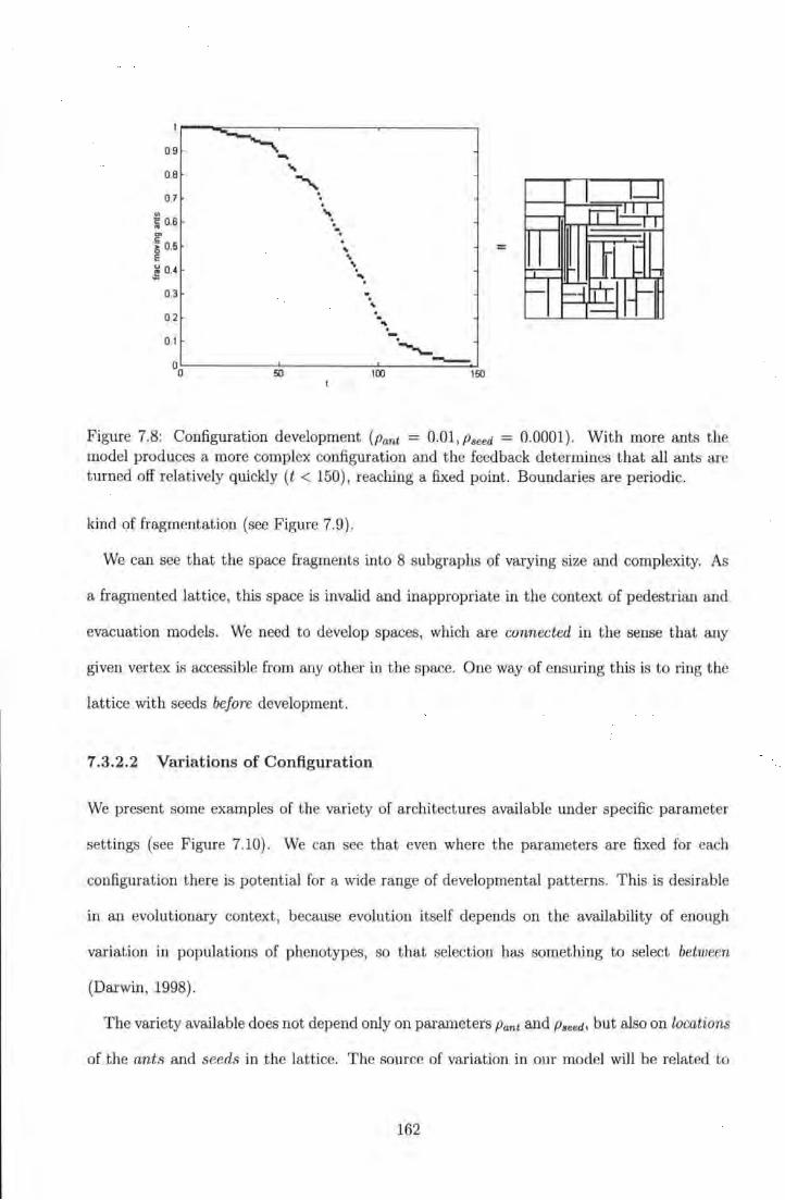
0.9

O.B

0.7 .. i 0.6

"' ·~ 0.5 E

~ 0.4

0.3

0.2

0.1

"' . . . . . ... .. .. . .... . .

... . . " . -.

-"'---0o~---------~L----------,OOL-----~==~,~

=

Figure 7.8: Configuration development (Pant = 0.01, Pseed = 0.0001) . With more ants the model produces a more complex configuration and the feedback determines that all ants are turned off relatively quickly (t < 150), reaching a fixed point. Boundaries are periodic.

kind of fragmentation (see Figure 7.9) .

We can see that the space fragments into 8 subgraphs of varying size and complexity. As

a fragmented lattice, this space is invalid and inappropriate in the context of pedestrian and

evacuation models. We need to develop spaces, which are connected in the sense that any

given vertex is accessible from any other in the space. One way of ensuring this is to ring the

lattice with seeds before development.

7.3.2.2 Variations of Configuration

We present some examples of the variety of architectures available under specific parameter

settings (see Figure 7.10) . We can see that even where the parameters are fixed for each

configuration there is potential for a wide range of developmental patterns. T his is desirable

in an evolutionary context, because evolution itself depends on the availability of enough

variation in populations of phenotypes, so that selection has something to select between

(Darwin, 1998).

The variety available does not depend only on parameters Pant and Pseed, but also on locations

of the ants and seeds in the lattice. The source of variation in our model will be related to

162

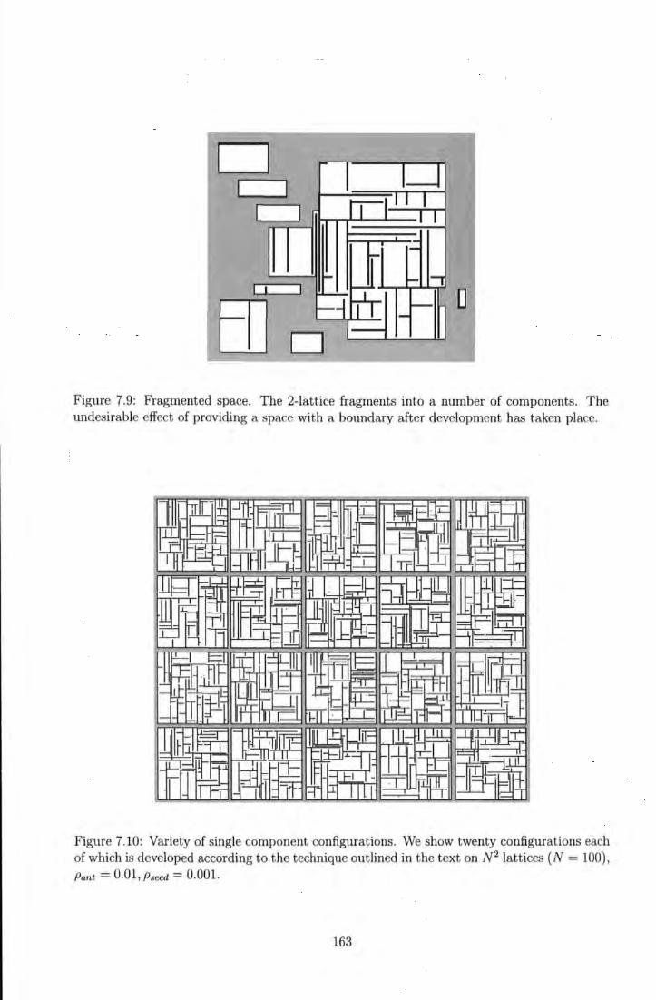
D

EO D D

Figure 7.9: Fragmented space. The 2-lattice fragments into a number of components. The undesirable effect of providing a space with a botmdary after development has taken place.

Figure 7.10: Variety of single component configurations. We show twenty configurations each of which is developed according to the technique outlined in the text on N 2 lattices (N = 100), Pant = 0.01 , Pseed = 0.001.

163

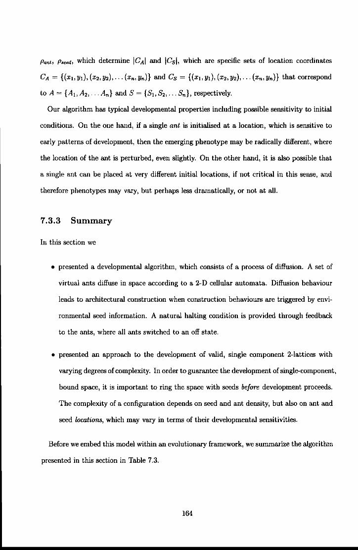
Pant> PswJ, which determine ICAI and ICsl, which are specific sets of location coordinates

CA = {(xl> yi), (x2, Y2), ... (xn, Yn)} and Cs = {(xi, yi), (x2, Y2), ... (xn, YnH that correspond

to A= {AI, A2, ... An} and S ={SI, S2, ... Sn}, respectively.

Our algorithm has typical developmental properties including possible sensitivity to initial

conditions. On the one hand, if a single ant is initialised at a location, which is sensitive to

early patterns of development, then the emerging phenotype may be radically different, where

the location of the ant is perturbed, even slightly. On the other hand, it is also possible that

a single ant can be placed at very different initial locations, if not critical in this sense, and

therefore phenotypes may vary, but perhaps less dramatically, or not at all.

7.3.3 Summary

In this section we

• presented a developmental algorithm, which consists of a process of diffusion. A set of

virtual ants diffuse in space according to a 2-D cellular automata. Diffusion behaviour

leads to architectural construction when construction behaviours are triggered by envi

ronmental seed information. A natural halting condition is provided through feedback

to the ants, where all ants switched to an off state.

• presented an approach to the development of valid, single component 2-lattices with

vBiying degrees of complexity. In order to guBiantee the development of single-component,

bound space, it is important to ring the space with seeds before development proceeds.

The complexity of a configuration depends on seed and ant density, but also on ant and

seed locations, which may vBiy in terrns of their developmental sensitivities.

Before we embed this model within an evolutionary framework, we summBiize the algorithm

presented in this section in Table 7.3.

164

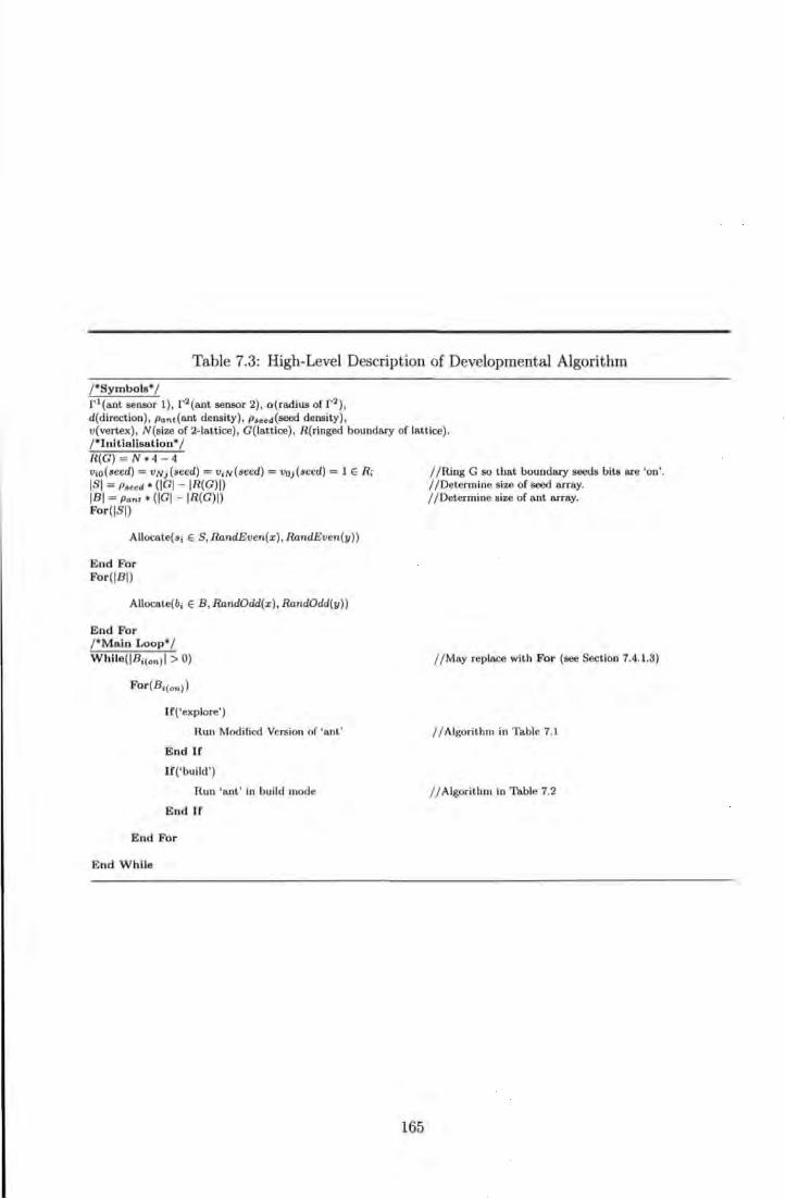
Table 7.3: High-Level Description of Developmental Algorithm

r symbols•;

r 1 (ant sensor 1), r 2 (ant sensor 2), a { radius of r 2 ) ,

d{direction), Ponc(ant density), P•eed{seed density) , v(vertex), N{size of 2-latt ice), G(latt ice), R{ringed boundary of lattice) . r initia!isation• 1 R(G) = N•4 -4 v;o{seed) = VN;(seed) = v;N(seed) = vo;(seed) = 1 E R; ISI = Pmd • {IGI - IR{G)I) IBI =Pant • {IGI- IR{G)I) For(ISI)

Allocate{ a; E S, RandEven(x) , RandEven(y))

End For For(IBI)

Allocate{b; E B , RandOdd(x) , RandOdd(y))

End For r Main Loop* I While{IB;(on) I > 0)

For(BI(on))

If{'explore')

Run Modified Version of 'ant'

End If

If{' build')

Run 'ant ' in build mode

End If

End For

End While

165

/ / lling G so tbat boundary seeds bits are 'on'. //Determine size of seed array. //Determine size of ant array.

//May replace with For (see Section 7.4.1.3)

//Algorithm in Table 7. 1

/ / Algorithm in Table 7.2

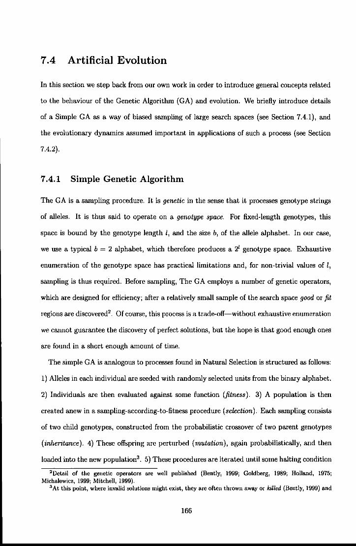
7.4 Artificial Evolution

In this section we step back from our own work in order to introduce general concepts related

to the behaviour of the Genetic Algorithm (GA) and evolution. We briefly introduce details

of a Simple GA as a way of biased sampling of large search spaces (see Section 7.4.1), and

the evolutionary dynamics assumed important in applications of such a process (see Section

7.4.2).

7.4.1 Simple Genetic Algorithm

The GA is a sampling procedure. It is genetic in the sense that it processes genotype strings

of alleles. It is thus said to operate on a genotype space. For fixed-length genotypes, this

space is bound by the genotype length l, and the size b, of the allele alphabet. In our case,

we use a typical b = 2 alphabet, which therefore produces a 21 genotype space. Exhaustive

enumeration of the genotype space has practical limitations and, for non-trivial values of l,

sampling is thus required. Before sampling, The GA employs a number of genetic operators,

which are designed for efficiency; after a relatively small sample of the search space good or fit

regions are discovered2 . Of course, this process is a trade-off-without exhaustive enumeration

we cannot guarantee the discovery of perfect solutions, but the hope is that good enough ones

are found in a short enough amount of time.

The simple GA is analogous to processes found in Natural Selection is structured as follows:

1) Alleles in each individual are seeded with randomly selected units from the binary alphabet.

2) Individuals are then evaluated against some function (fitness). 3) A population is then

created anew in a sampling-according-to-fitness procedure (selection). Each sampling consists

of two child genotypes, constructed from the probabilistic crossover of two parent genotypes

(inheritance). 4) These offspring are perturbed (mutation), again probabilistically, and then

loaded into the new population3 . 5) These procedures are iterated until some halting condition

2Detail of the genetic operators are well published (Bently, 1999; Goldberg, 1989; Holland, 1975; Michalewicz, 1999; Mitchell, 1999).

3 At this point, where invalid solutions might exist, they are often thrown away or killed (Bently, 1999) and

166

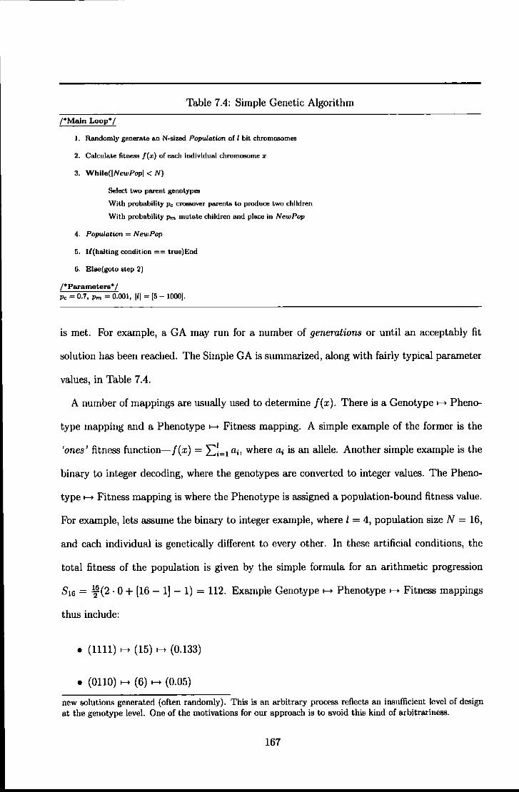
Table 7.4: Simple Genetic Algorithm

/*Main Loop• I

1. Randomly generate an N·sized Population of l bit chromosomes

2. Calculate fitness f(x) of each individual chromosome x

3. Whlla([NewPop[ < N)

Select two parent genotypes

With probability Pc crossover parents to produce two children

With probability Pm mutate children aod place in NewPop

4. Population = NewPop

5. If(halting condition == true)End

6. Else(goto step 2)

/*Parameters• I Pc = 0.7, Pm = 0.001, [I[ = [5- 1000[.

is met. For example, a GA may run for a number of generations or until an acceptably fit

solution has been reached. The Simple GA is summarized, along with fairly typical parameter

values, in Table 7.4.

A number of mappings are usually used to determine f(x). There is a Genotype>--> Pheno-

type mapping and a Phenotype >--> Fitness mapping. A simple example of the former is the

'ones' fitness function-/(:~;)= L::=l a;, where a; is an allele. Another simple example is the

binary to integer decoding, where the genotypes are converted to integer values. The Pheno-

type >--> Fitness mapping is where the Phenotype is assigned a population-bound fitness value.

For example, lets assume the binary to integer example, where l = 4, population size N = 16,

and each individual is genetically different to every other. In these artificial conditions, the

total fitness of the population is given by the simple formula for an arithmetic progression

S16 = ~(2 · 0 + [16- 1]- 1) = 112. Example Genotype>--> Phenotype>--> Fitness mappings

thus include:

• (1111) ...... (15) ...... (0.133)

• (0110) ...... (6) ...... (0.05)

new solutions generated (often randomly). This is an arbitrary process reflects an insufficient level of design at the genotype level. One of the motivations for our approach is to avoid this kind of arbitrariness.

167

-f(x) __.

Figure 7.11: Fitness landscape. Each point on a four-dimensional hypercube corresponds to a genotype, which is mapped onto a phenotype value. Three different phenotypes are highlighted by a circle, the size of which corresponds to fitness .

• (1100) r-t (12) r-t (0.107)

These mapping can be visualised in the form of a four-dimensional hypercube (see Figure

7.11).

7.4.2 Evolutionary D ynamics

After the Genotype r-t Phenotype r-t Fitness mapping is specined, the entire genotype space

can then be pictured by analogy to a fitness landscape (Wright, 1932). In our example, we only

present 4-bit genotypes, but the landscape analogy is often reffered to in many dimensions.

With this picture in mind, the population is more or less converged on a region of the landscape

where the relative peaks and troughs represent genotypes of varying fitness values. The

crossover and mutation operators explore genotype space and uphill moves are reinforced

through the process of selection. The evolutionary dynamics therefore tend to drive the

population into areas of progressively higher fitness peaks. In the above sense, the aim of

using the GA is to maximise fitness4 .

In the example mapping provided, the genotypes all map to different phenotypes. Any

4 In other applications however, f(x) may be designed to minimise energy-in combinatorial optimisation problems this is often the case.

168

genetic change in a genotype will therefore correspond to a change in fitness. Such an example

is at odds with the neutral theory of evolution, which claims that many genetic changes are

maintained because selection does not have the power to distinguish between various genotypes

with similar, but not identical fitness values. On this view, properties in the phenotype

can therefore result from neutral genetic drift rather than selection (Kimura, 1983). The

more traditional selectionist paradigm in evolutionary theory has underpinned much work

in artificial evolution. Unlike the example provided, artificial Genotype ...... Phenotype ......

Fitness mappings will almost certainly contain neutrality, but only as an unintended side effect,

rather than being intended as a potential adaptive property of the genotype. Only relatively

recently has the role of neutrality been taken seriously in the context of artificial adaptation.

Genotype ...... Fitness mappings, which introduce beneficial neutrality into the search space,

have important general implications for artificial evolution as a whole. Investigations into such

mappings have exploited the self-organising properties of CA (For example, Shipman, 2003).

It is therefore important to mention that the CA mapping used in this thesis has not been

investigated along these lines of enquiry, but used only in the context of advantages already

outlined above5 . Having briefly outlined the GA and general conceptions of evolutionary

dynamics, we now outline the use of our generative algorithm as a mapping in an evolutionary

context.

7.5 Evolution: Generative Architecture

This is the first section of this thesis where we attempt to bring together all the methods pre-

sented previously in an approach to evolutionary design. We present a genetic encoding and

how this (with the use of our developmental algorithm) maps to phenotypes (Section 7.5.1).

We then present the details of the genetic algorithm used (Section 7.5.2). We present de-

tails of the phenotype-fitness mapping (Section 7.5.3) and show results from an evolutionary

5This is not to say that work in the area of Neutral Networks is not important to our concerns. Open-ended evolution is a desirable property for all Evolutionary Algorithm applications. However, research in thls area is in early stages of investigation and beyond the scope of this thesis.

169

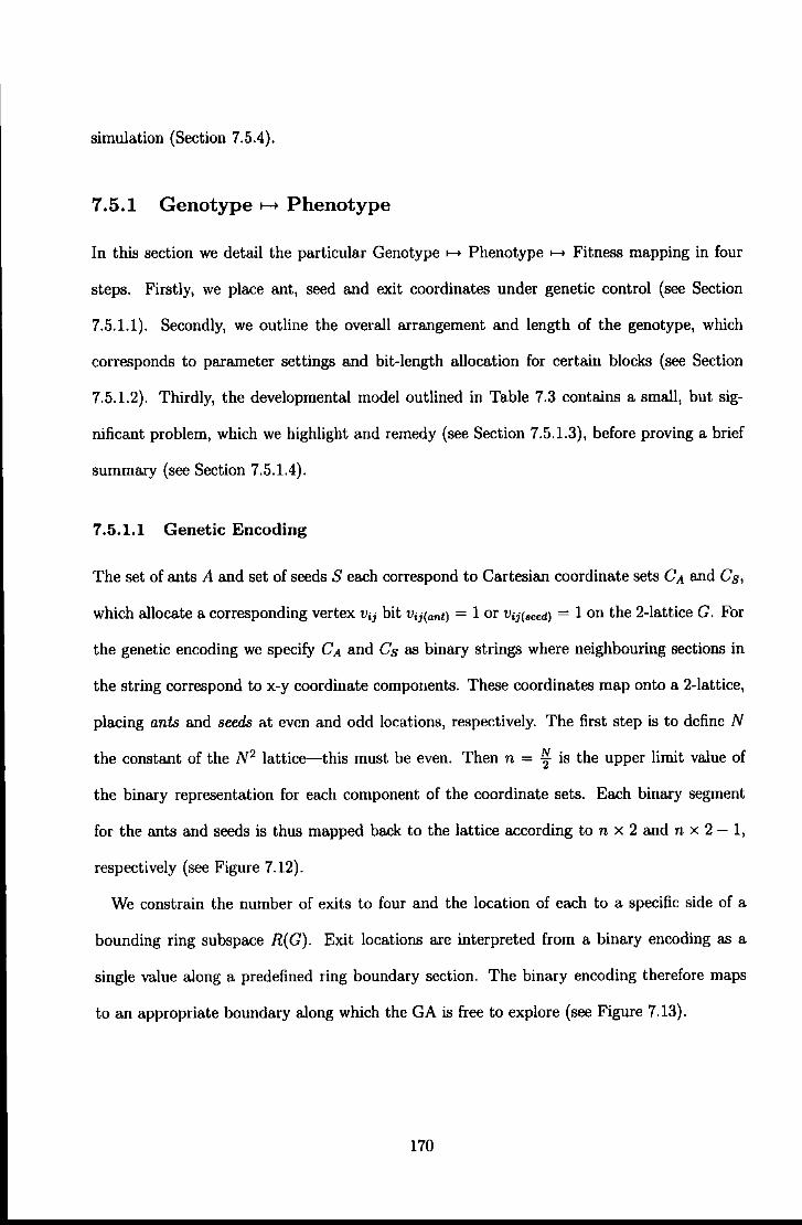
simulation (Section 7.5.4).

7.5.1 Genotype f-> Phenotype

In this section we detail the particular Genotype f-> Phenotype f-> Fitness mapping in four

steps. Firstly, we place ant, seed and exit coordinates under genetic control (see Section

7.5.1.1). Secondly, we outline the overall arrangement and length of the genotype, which

corresponds to parameter settings and bit-length allocation for certain blocks (see Section

7.5.1.2). Thirdly, the developmental model outlined in Table 7.3 contains a small, but sig

nificant problem, which we highlight and remedy (see Section 7.5.1.3), before proving a brief

summary (see Section 7.5.1.4).

7.5.1.1 Genetic Encoding

The set of ants A and set of seeds S each correspond to Cartesian coordinate sets CA and Cs,

which allocate a corresponding vertex V;j bit Vij(ant) = 1 or V;j(seed) = 1 on the 2-lattice G. For

the genetic encoding we specify CA and Cs as binary strings where neighbouring sections in

the string correspond to x-y coordinate components. These coordinates map onto a 2-lattice,

placing ants and seeds at even and odd locations, respectively. The first step is to define N

the constant of the N 2 lattice-this must be even. Then n = If is the upper limit value of

the binary representation for each component of the coordinate sets. Each binary segment

for the ants and seeds is thus mapped back to the lattice according to n x 2 and n x 2- 1,

respectively (see Figure 7.12).

We constrain the number of exits to four and the location of each to a specific side of a

bounding ring subspace R(G). Exit locations are interpreted from a binary encoding as a

single value along a predefined ring boundary section. The binary encoding therefore maps

to an appropriate boundary along which the GA is free to explore (see Figure 7.13).

170

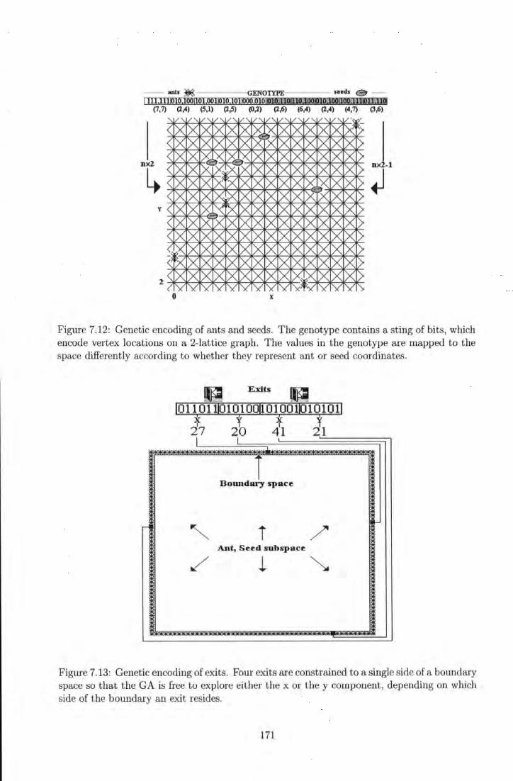
ants ~ GENOTYPE seeds (3 -l lll.lllK!lo.Ioollol.ooll!lo.IolOO)J)loiQIOJlOI110JOOIUOJ!!OillJQ.ll11!11.1lQ

(7, 7) (2,4) (5,1) (2,5) (O,l) (2,6) (6,4) (2,4) (4, 7) (3,6)

nx2

l. y

0 X

Figure 7.12: Genetic encoding of ants and seeds. The genotype contains a sting of bits, which encode vertex locations on a 2-lattice graph. The values in the genotype are mapped to the space differently according to whether t hey represent ant or seed coordinates.

G Exits G IO 1101110101 00l10 100110101 01l * I * t 27 2b 41 21

I I

Bom1dary space

r ~ i /

Ant, Seed subspace

/ l ~

Figure 7.13: Genetic encoding of exits. Four exits are constrained to a single side of a boundary space so that the GA is free to explore either the x or they component, depending on which side of the boundary an exit resides.

171

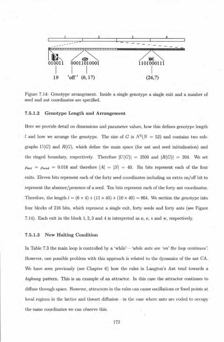
~~~~~~~~~~~~~ 1111111111111111111

lli?J"- e~ 010011 00011010001

731«~ 1101000111

I I I I 19 •off • (6, 17) (26,7)

Figure 7.14: Genotype arrangement. Inside a single genotype a single exit and a number of seed and ant coordinates are specified.

7.5.1.2 Genotype Length and Arrangement

Here we provide detail on dimensions and parameter values, how this defines genotype length

l and how we arrange the genotype. The size of G is N 2 (N = 52) and contains two sub-

graphs U(G) and R(G), which define the main space (for ant and seed initialisation) and

the ringed boundary, respectively. Therefore IU(G)I = 2500 and IR(G)I = 204. We set

Pant = Pseed = 0.016 and therefore IAI = ISI = 40. Six bits represent each of the four

exits. Eleven bits represent each of the forty seed coordinates including an extra on/off bit to

represent the absence/presence of a seed. Ten bits represent each of the forty ant coordinates.

Therefore, the length l = (6 x 4) + (11 x 40) + (10 x 40) = 864. We section the genotype into

four blocks of 216 bits, which represent a single exit, forty seeds and forty ants (see Figure

7.14). Each exit in t he block 1, 2, 3 and 4 is interpreted as n, e, s and w, respectively.

7.5.1.3 New Halting Condition

In Table 7.3 the main loop is controlled by a 'while'-'while ants are 'on' the loop continues'.

However, one possible problem with this approach is related to the dynamics of the ant CA.

We have seen previously (see Chapter 6) how the rules in Langton's Ant tend towards a

highway pattern. This is an example of an attractor. In this case the attractor continues to

diffuse through space. However, attractors in the rules can cause oscillations or fixed points at

local regions in the lattice and thwart diffusion- in the case where ants are coded to occupy

the same coordinates we can observe this.

172

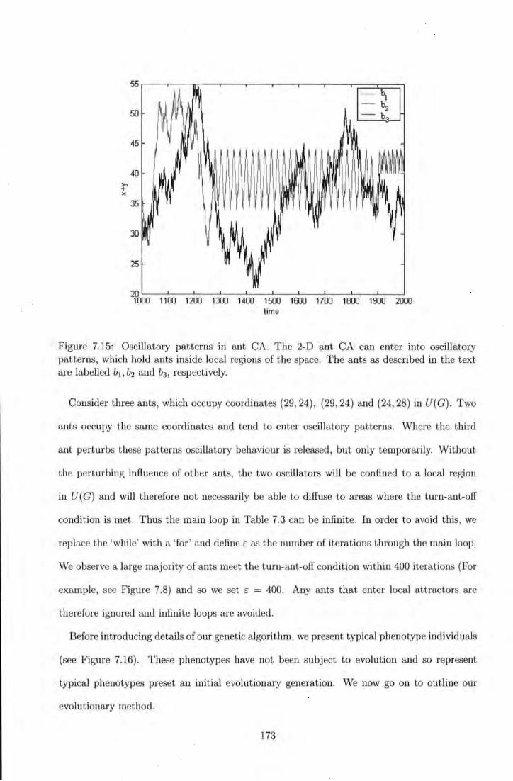
55

- b 50 2

-b

45

40 ,..., + )(

35

30

25

20~--~--~--~---L--~---J--~L---~--J---~ 1000 1100 1200 1300 1400 1500 1600 1700 1800 1900 2000

time

Figure 7.15: Oscillatory patterns in ant CA. The 2-D ant CA can enter into oscillatory patterns, which hold ants inside local regions of the space. The ants as described in the text are labelled b1, b2 and b3 , respectively.

Consider three ants, which occupy coordinates (29, 24) , {29, 24) and (24, 28) in U(G). Two

ants occupy the same coordinates and tend to enter oscillatory patterns. Where the third

ant perturbs these patterns oscillatory behaviour is released, but only temporarily. Without

the perturbing influence of other ants, the two oscillators will be confined to a local region

in U (G) and will therefore not necessarily be able to diffuse to areas where the turn-ant-off

condition is met. Thus the main loop in Table 7.3 can be infinite. In order to avoid this, we

replace the 'while' with a 'for ' and define cas the number of iterations through the main loop.

We observe a large majority of ants meet the turn-ant-off condition within 400 iterations (For

example, see Figure 7.8) and so we set c = 400. Any ants that enter local attractors are

therefore ignored and infinite loops are avoided.

Before introducing details of our genetic algorithm, we present typical phenotype individuals

(see Figure 7.16). These phenotypes have not been subject to evolution and so represent

typical phenotypes preset an initial evolutionary generation. We now go on to outline our

evolutionary method.

173

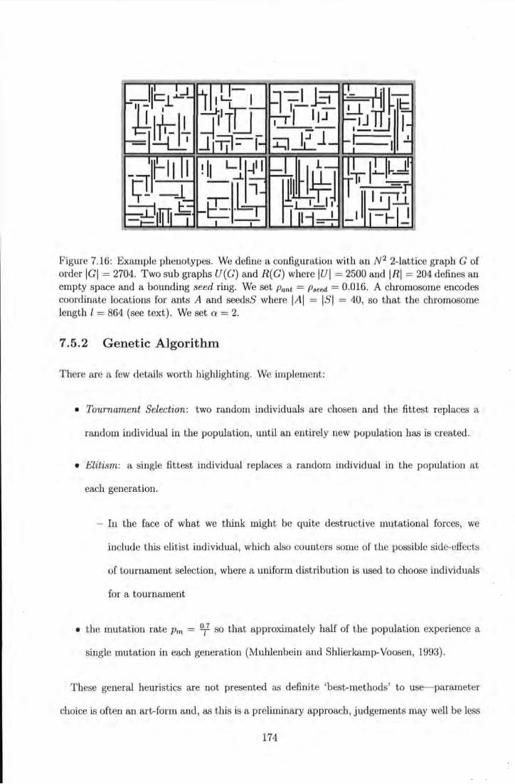
Figure 7.16: Example phenotypes. We define a configuration with an N2 2-lattice graph G of order IGI = 2704. Two sub graphs U(G) and R(G) where IUI = 2500 and IRI = 204 defines an empty space and a bounding seed ring. We set Pant= Pseed. = 0.016. A chromosome encodes coordinate locations for ants A and seedsS where IAI = ISI = 40, so that the chromosome length l = 864 (see text). We set a= 2.

7.5.2 Genetic Algorithm

There are a few details worth highlighting. We implement:

• Tournament Selection: two random individuals are chosen and the fittest replaces a

random individual in the population, until an entirely new population has is created.

• Elitism: a single fittest individual replaces a random individual in the population at

each generation.

- In the face of what we think might be quite destructive mutational forces, we

include this elitist individual, which also counters some of the possible side-effects

of tournament selection, where a uniform distribution is used to choose individuals

for a tournament

• the mutation rate Pm = 0i7 so that approximately half of the population experience a

single mutation in each generation (Muhlenbein and Shlierkamp-Voosen, 1993) .

These general heuristics are not presented as definite 'best-methods' to use-parameter

choice is often an art-form and, as this is a preliminary approach, judgements may well be less

174

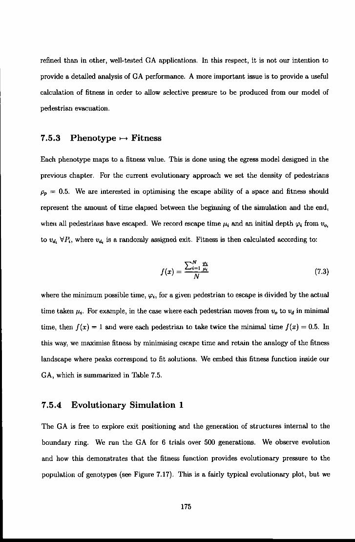
refined than in other, well-tested GA applications. In this respect, it is not our intention to

provide a detailed analysis of GA performance. A more important issue is to provide a useful

calculation of fitness in order to allow selective pressure to be produced from our model of

pedestrian evacuation.

7.5.3 Phenotype ..-. Fitness

Each phenotype maps to a fitness value. This is done using the egress model designed in the

previous chapter. For the current evolutionary approach we set the density of pedestrians

Pp = 0.5. We are interested in optimising the escape ability of a space and fitness should

represent the amount of time elapsed between the beginning of the simulation and the end,

when all pedestrians have escaped. We record escape time 1-li and an initial depth cp; from v0 ,

to vd; V P;, where vd; is a randomly assigned exit. Fitness is then calculated according to:

""N !& f (X) = L...,i=l p;

N (7.3)

where the minimum possible time, cp;, for a given pedestrian to escape is divided by the actual

time takeni-Li. For example, in the case where each pedestrian moves from V0 to vd in minimal

time, then f(x) = 1 and were each pedestrian to take twice the minimal time f(x) = 0.5. In

this way, we maximise fitness by minimising escape time and retain the analogy of the fitness

landscape where peaks correspond to fit solutions. We embed this fitness function inside our

GA, which is summarized in Table 7.5.

7.5.4 Evolutionary Simulation 1

The GA is free to explore exit positioning and the generation of structures internal to the

boundary ring. We run the GA for 6 trials over 500 generations. We observe evolution

and how this demonstrates that the fitness function provides evolutionary pressure to the

population of genotypes (see Figure 7.17). This is a fairly typical evolutionary plot, but we

175

Table 7.5: Our Genetic Algorithm

/"Main Loop• I

I. Randomly generate an N-sized Population of I bit genotypes

2. Develop N phenotypes 8CCOrding to the procedure outlined in Table 7.3

3. Calculate fitness /(z) of each genotype "' according to Equation 7.2

4. Whlle(INewPopl < N)

Select two parent genotypes according to tournament selection (tournament size = 2) with replacement.

With probability p, crossover parents to produce two children

With probability p, mutate children and place in New Pop

End While

5. Overwrite an individual in NewPop with be8t from popualtion

6. Population= New Pop

7. If(generati0718 = 0)

HALT

End If

B. Else

generations = generations - 1

(goto step 2)

End Else

r Par&Ineters• I p, = 0.7, Pm = !lf!, Ill= 8&1, N = 100, generations= 500.

176

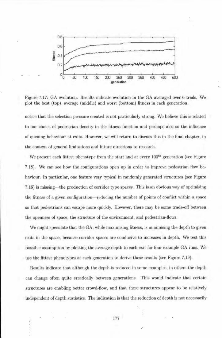
0.8

0.6 (/) (/) Q) 0.4 c: ~

0.2

50 1 00 150 200 250 300 350 400 450 500 generation

Figure 7.17: GA evolution. Results indicate evolution in the GA averaged over 6 trials. We plot the best (top), average (middle) and worst (bottom) fitness in each generation.

notice that the selection pressure created is not particularly strong. We believe this is related

to our choice of pedestrian density in the fitness function and perhaps also so the influence

of queuing behaviour at exits. However, we will return to discuss this in the final chapter, in

the context of general limitations and future directions to research.

We present each fittest phenotype from the start and at every lOOth generation (see Figure

7.18). We can see how the configurations open up in order to improve pedestrian flow be-

haviour. In particular, one feature very typical in randomly generated structures (see Figure

7.16) is missing- the production of corridor type spaces. This is an obvious way of optimising

the fitness of a given configuration- reducing the number of points of conflict within a space

so that pedestrians can escape more quickly. However, there may be some trade-off between

the openness of space, the structure of the environment, and pedestrian-flows.

We might speculate that the GA, while maximising fitness, is minimising the depth to given

exits in the space, because corridor spaces are conducive to increases in depth. We test this

possible assumption by plotting the average depth to each exit for four example GA runs. We

use the fittest phenotypes at each generation to derive these results (see Figure 7.19).

Results indicate that although the depth is reduced in some examples, in others the depth

can change often quite erratically between generations. This would indicate that certain

structures are enabling better crowd-flow, and that these structures appear to be relatively

independent of depth statistics. The indication is that the reduction of depth is not necessarily

177

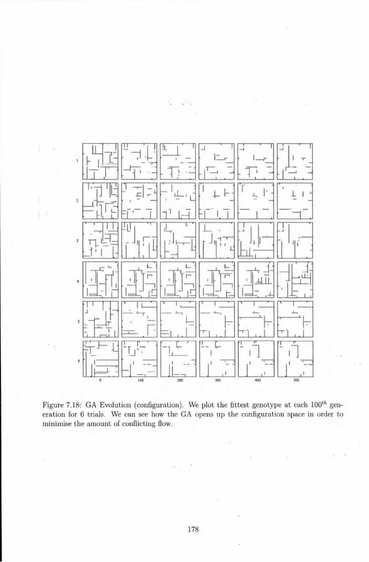
Figure 7.18: GA Evolution (configuration). We plot the fittest genotype at each lOOth generation for 6 trials. We can see how the GA opens up the configuration space in order to minimise the amount of conflicting flow.

178

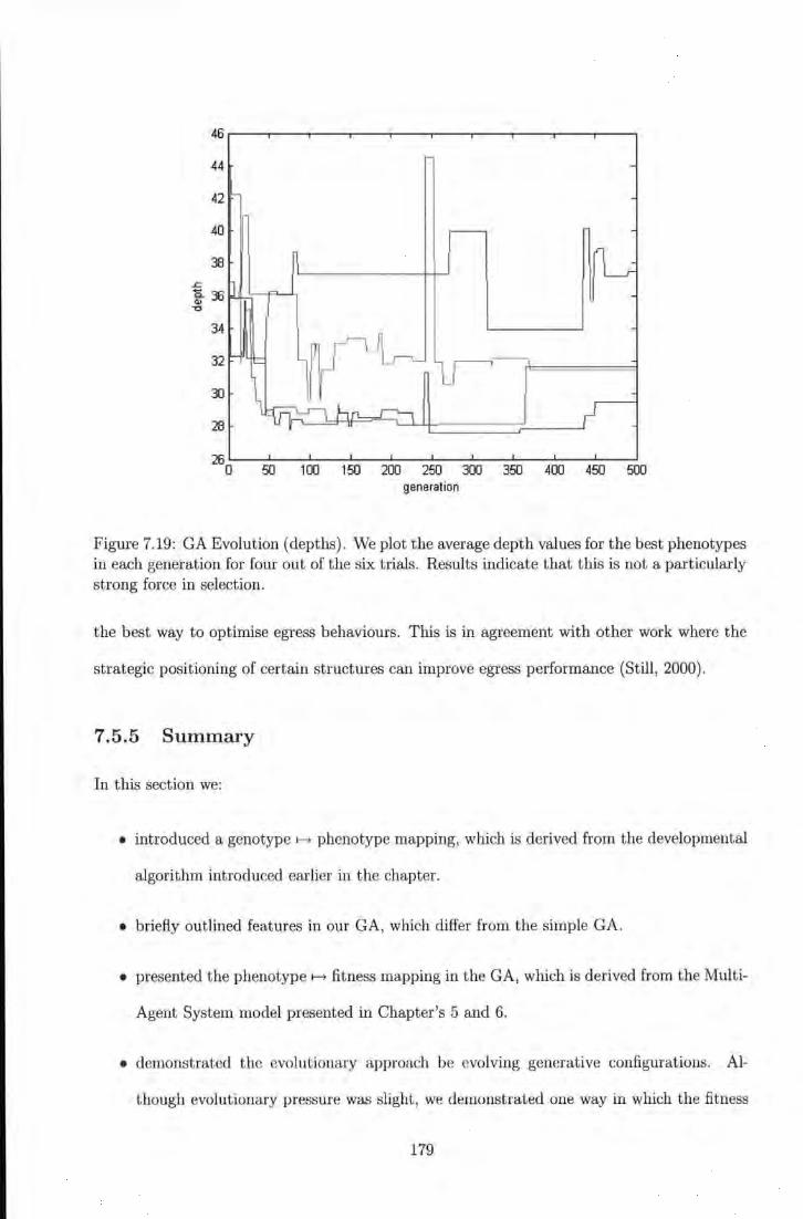
44

42

40

38

34

32

30

28

260 50 1 00 150 200 250 300 350 400 450 500 generation

Figure 7.19: GA Evolution (depths). We plot the average depth values for the best phenotypes in each generation for four out of the six trials. Results indicate that this is not a particularly strong force in selection.

the best way to optirnise egress behaviours. This is in agreement with other work where the

strategic positioning of certain structures can improve egress performance (Still, 2000).

7.5.5 Summary

In this section we:

• introduced a genotype f-4 phenotype mapping, which is derived from the developmental

algorithm introduced earlier in the chapter.

• briefly outlined features in our GA, which differ from the simple GA.

• presented the phenotype f-4 fitness mapping in the GA, which is derived from the Multi-

Agent System model presented in Chapter's 5 and 6.

• demonstrated the evolutionary approach be evolving generative configurations. Al-

though evolutionary pressure was slight, we demonstrated one way in which the fitness

179

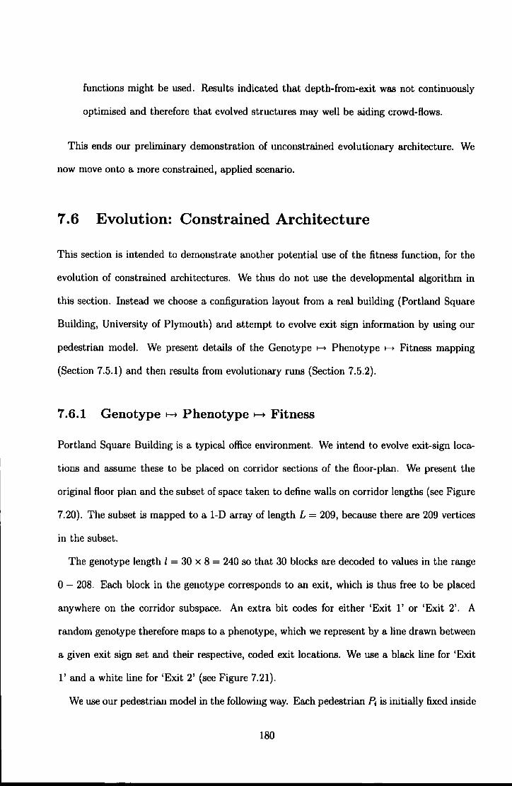
functions might be used. Results indicated that depth-from-exit was not continuously

optimised and therefore that evolved structures may well be aiding crowd-flows.

This ends our preliminary demonstration of unconstrained evolutionary architecture. We

now move onto a more constrained, applied scenario.

7.6 Evolution: Constrained Architecture

This section is intended to demonstrate another potential use of the fitness function, for the

evolution of constrained architectures. We thus do not use the developmental algorithm in

this section. Instead we choose a configuration layout from a real building (Portland Square

Building, University of Plymouth) and attempt to evolve exit sign information by using our

pedestrian model. We present details of the Genotype >-+ Phenotype >-+ Fitness mapping

(Section 7.5.1) and then results from evolutionary runs (Section 7.5.2).

7.6.1 Genotype~ Phenotype~ Fitness

Portland Square Building is a typical office environment. We intend to evolve exit-sign loca

tions and assume these to be placed on corridor sections of the floor-plan. We present the

original floor plan and the subset of space taken to define walls on corridor lengths (see Figure

7.20). The subset is mapped to a 1-D array of length L = 209, because there are 209 vertices

in the subset.

The genotype length l = 30 x 8 = 240 so that 30 blocks are decoded to values in the range

0 - 208. Each block in the genotype corresponds to an exit, which is thus free to be placed

anywhere on the corridor subspace. An extra bit codes for either 'Exit 1' or 'Exit 2'. A

random genotype therefore maps to a phenotype, which we represent by a line drawn between

a given exit sign set and their respective, coded exit locations. We use a black line for 'Exit

1' and a white line for 'Exit 2' (see Figure 7.21).

We use our pedestrian model in the following way. Each pedestrian P; is initially fixed inside

180

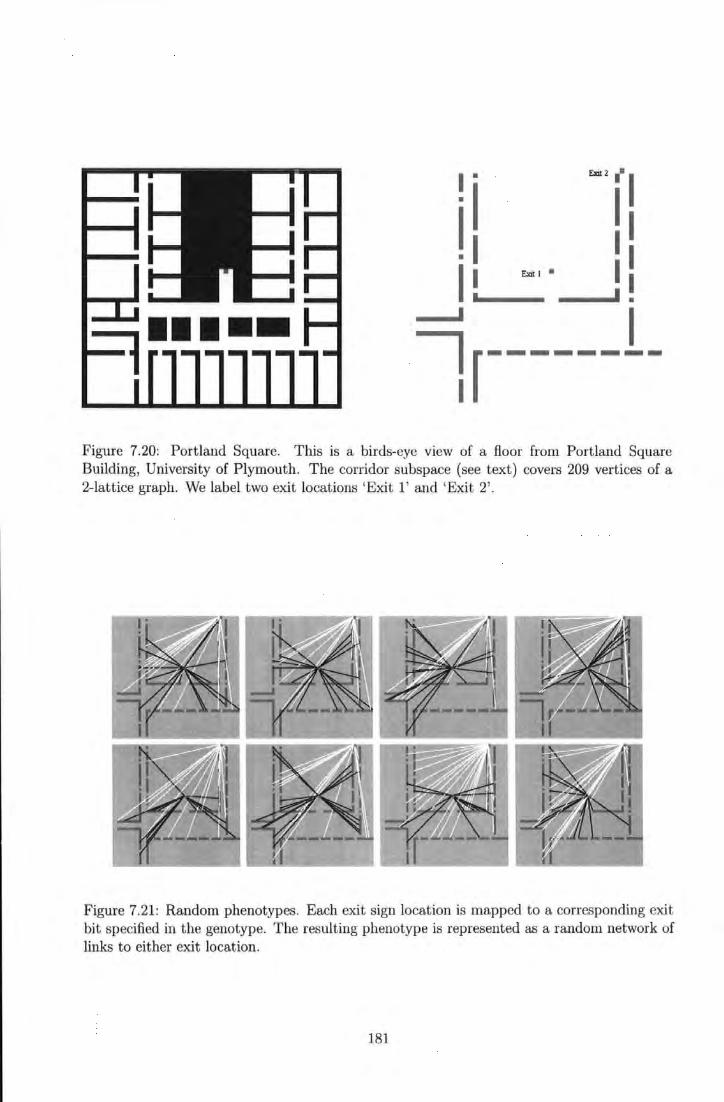
I. Exit 2··~

i I 11 1 ... 1 -Ezt-' l • _ ... ! !

I lr--------I

Figure 7.20: Portland Square. This is a birds-eye view of a floor from Portland Square Building, University of Plymouth. The corridor subspace (see text) covers 209 vertices of a 2-lattice graph. We label two exit locations 'Exit 1' and 'Exit 2'.

Figure 7.21: Random phenotypes. Each exit sign location is mapped to a corresponding exit bit specified in the genotype. The resulting phenotype is represented as a random network of links to either exit location.

181

one of the 27 rooms (2 pedestrians per room). The size of the pedestrian population is thus

54. Each pedestrian moves randomly until an exit sign is detected in a Moore neighbourhood

f;. On detecting an exit sign, vd, is then set to the vertex specified by the bit of the genotype,

which maps to either 'Exit 1' or 'Exit 2'. The pedestrian can then begin moving towards the

exit as indicated by our model. Fitness is calculated in the manner given in Equation 7.2.

7.6.2 Evolutionary Simulation 2

We run 8 trials of the GA, which is the same as the one given in Table 7.5, other than the

details outlined in this section. The parameters in the ga are: Pc = 0. 7, Pm = 0/, l =

240, N = 100, generatians = 500 ..

We present evolutionary results, which again show the effect of selection over time (see Fig

ure 7.22). We present two example trials in order to show the effect of the random walking

in the model, which introduced noise into the fitness function. However, even with this noise,

evolution takes hold and fit phenotypes develop. We also present these phenotypes (see Fig

ure 7.23). Notice how the population of exit-signs is split between the two exits in each

trial. The pattern of split is such that pedestrians tend to move towards the closest exit, but

also pedestrians moving to different exits avoid each other and conflict in the population is

minimised.

7.7 Summary

In this chapter we:

• reviewed two models of aggregative growth systems in nature.

• developed an algorithm for the automatic generation of valid, single component labyrinthine

configurations.

• presented a method of how to use the algorithm in an evolutionary context as a compo

nent in Genotype 1-+ Phenotype 1-+ Fitness mappings.

182

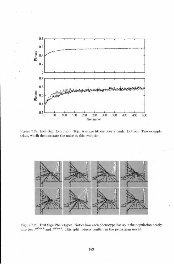
0.8

0.6 Ill Ill Q) 0.4 c:

.t:: LL..

0.2

0

0.7

0.6 Ill Ill Q) 0.5 c:

.t:: LL..

0.4

~

50 100 150 200 250 300 350 400 450 500 Generation

Figure 7.22: Exit Sign Evolution . Top: Average fitness over 8 trials. Bottom: Two example trials, whcih demonstrate the noise in this evolution .

Figure 7.23: Exit Sign Phenotypes. Notice how each phenotype has split the population neatly into two pE:tit 1 and pExit 2 . This split reduces conflict in t he pedestrian model.

183

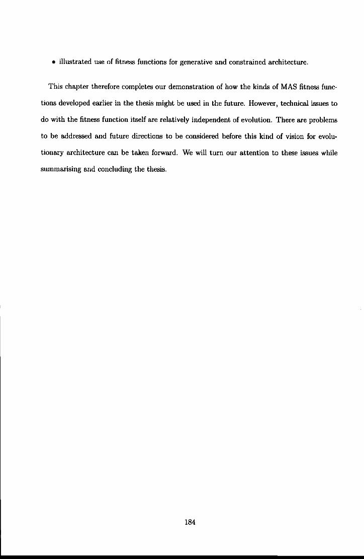
• illustrated use of fitness functions for generative and constrained architecture.

This chapter therefore completes our demonstration of how the kinds of MAS fitness func

tions developed earlier in the thesis might be used in the future. However, technical issues to

do with the fitness function itself are relatively independent of evolution. There are problems

to be addressed and future directions to be considered before this kind of vision for evolu

tionary architecture can be taken forward. We will turn our attention to these issues while

summarising and concluding the thesis.

184

Chapter 8

Conclusion

Our long-term objective is to design fitness functions, which introduce useful selective forces,

for an evolutionary approach to architectural design. There were two main strands of research,

1) fitness function definition and 2) an evolutionary approach. The first strand defines the

core work in this thesis, where we have concentrated on the development of techniques for

the design of egress models. We review the important contributions of the thesis (see Section

8.1), before outlining future directions of research (see Section 8.2). Finally, we provide some

closing comments to the thesis (see Section 8.3).

8.1 Thesis Summary

8.1.1 Background: Crowd Dynamics

In order to begin thinking about the problem of fitness function definition, we investigated

existing techniques from the pedestrian and evacuation modelling community (Chapter's 2 and

3). All of the techniques had limitations, but those based the Multi-Agent System concept

used an appropriate level of abstraction-simulation models where patterns emerge through

unfolding dynamics-which allow important interactions to be represented.

Given the requirements of labyrinthine spatial complexity, models based on discrete space

185

were subject to further review. These models implicitly use a 2-lattice graph. After defining

important features of this graph, discrete models were reviewed in more depth. Two general

methods, which capture two separate levels appeared promising:

• Cellular Automata (CA)

- local dynamics

• Attractor Fields

- global dynamics

8.1.2 Limits to Locality: Percolation

Chapter 4 is the point where the core work in this thesis began. We replicated a number of

CA models. The first (Nagel and Rasmussen, 1994) allowed us to gain an understanding of

the interactive properties of lattice spaces. In the 1-lattice, interactions can be said to ripple

over time. At critical parameter values, random driver effects can have affect other drivers

who are much further away, but at a later point in time.

These chains of interdependence are best appreciated by looking at the statistical dynam

ics of a model. However, what you see depends on the statistics you choose to observe.

Publications on another model, the pedestrian CA (Blue and Adler, 2000a), include average

speed-density relationships, which appear unproblematic at face value. We endeavored to

gain a fuller understanding of these models by looking at alternative statistical properties and

performing an in-depth investigation of the dynamics. Statistical results were complemented

by more qualitative observations. Both revealed breakdowns in self-organisation in the face

of increasing density. Also, rather than steady deterioration, breakdown was sudden.

One particular experiment revealed underlying patterns of randomness in different popula

tions of pedestrians, which later (Chapter 5) was revealing in the light of 2-lattice percolation

statistics. But perhaps this behaviour could have been due to the internal logic of local rule

sets? We attempted to investigate this question and control some of the inherent randomness.

186

We also attempted to investigate local dynamics with a view to using them in an attractor

field context, with the aim of integrating the two separate levels. We failed however, and

dynamics remained brittle at unacceptably low density values.

The persistent and catastrophic nature of model failure provided a clue as to what was

happening. It is known in other areas of graph theory that random edge connections between

vertices in a graph undergo phase transitions-sudden, global changes in connectivity with

the formation of giant-component clustering (Barabsi, 2002; Watts, 1999; Kauffman, 1995).

Could it be that clustering properties were also responsible for the phase transitions observed

in the CA?

We argued that 1-D search components of the pedestrian CA, inherited from the 1-lattice

car CA, put unacceptable limitations on 2-lattice dynamics. Neighbourhoods were invaded by

the sudden emergence of percolation in the 2-lattice, which is analogous to the rippling effects

that take root in the car CA. This idea was supported by statistical results, which showed that

underlying patterns of randomness converge within critical density ranges, ripe for percolation.

These percolation effects are unintended and, rather than capturing interesting properties of

real systems, like the car CA, dynamics in the pedestrian CA produced nonsense.

8.1.3 Solution: Inclusive Search, Simple Dynamics

These investigations provided us with an empirical foundation on which to develop a new

approach to pedestrian and evacuation modelling. We aimed to provide a solution to the

brittle properties of local search and the non-responsive, fixed nature of attractor fields. This

solution was based on a more inclusive concept of search.

We proposed the use of a Pulse Coupled Neural Network as a candidate search algorithm,

because it automatically encapsulates inclusive search, where all paths away from a given

vertex origin can be searched until a specified destination is reached. This allowed us to move

model dynamics away from a purely local regions, and to increase model robustness to lattice

percolation. We investigated the PCNN and showed how best to arrange neuron equations

187

to produce clean, expanding autowaves, so that the neural plane could contain shortest-path,

traceback information. The PCNN is computationally expensive, but the complex behaviours

obtainable with simple network logic are a worthwhile trade-off.

In order to improve the trade-off, in Chapter 6, we presented a more efficient algorithm for

autowave generation. Pedestrians, it is generally assumed, make more or less local decisions,

but attempts to model these mechanisms in discrete space have failed. It is this previously

demonstrated, practical difficulty, which motivated inclusive search, rather than any abstract

philosophical stance towards human cognition vis d vis navigation. We believe that more

inclusive search is the best way to overcome the complex problems inherent to discrete updates

on the 2-lattice.

This approach also enables the specification of simple dynamic rules for model specification.

A dynamic is a rule, which processes the current state of a system and produces an updated

state. In our network-level tools, one rule goes as follows: explore every path away from a

given vertex to another vertex. Then: return the shortest path between the two vertices. With

these dynamics, we were primarily interested in producing higher-level patterns of emergence,

compatible with real observations of crowd populations. We demonstrated how other pedes

trians constrain network search and, accordingly, the way to model pedestrian interaction was

through a relaxation of these constraints, relative to movement directions.

At the end of Chapter 6, with this simple method, we replicated some higher-level patterns

found in real crowds. This was one of our main aims- to develop simple models of complex

crowd behaviour. We captured some of the local processes in pedestrian-pedestrian interac

tion, while also implementing longer-range egress behaviour. This compromise between local

and global dynamics is a particular strength of the methods, which are vindicated by the

production of more realistic results compared with other approaches.

188

8.1.4 Evolutionary Approach

The results justify the use of these methods in an evolutionary scenario. The aim of Chapter

7 was to provide a preliminary, motivating framework for evolutionary architecture. We

defined a Genotype ,_. Phenotype ,_. Fitness mapping. One of the main difficulties in coding

a genotype for a valid architectural configuration is to ensure that the resulting phenotype

space is not fragmented, i.e., that the lattice remains single-component.

We looked at models of nature-inspired growth to see if we could use any of the processes

assumed in natural architectural construction and, therefore, avoid the difficulty of having

to specify complex phenotypes in binary strings. The main motivation for this approach

was to design a developmental procedure, which acts as genetic-code container. Any of the

complexity in phenotype construction could then be handled by the container. The systems

that inspired our own-social insects and crystal growth-had some desirable algorithmic and

phenotypic properties. We attempted to incorporate these features into our own system.

Our algorithm consisted of two different growth agents-ants and seeds. We showed how

this approach could generate architectural spaces without fragmenting them. The method

also produced a large variety of forms, which thus met a second evolutionary requirement,

i.e., phenotypic variation. In order to map genotypes to variable phenotypes we then placed

two sources of phenotypic variation under genetic control.

Evolutionary simulations demonstrated fitness function pressure. In general it appeared

that the GA was evolving to spaces of least depth, but further results suggested that the

presence of obstacles within the space might be beneficial for an egress scenario; the statistic

of average depth was seen to be largely unimportant in the evolution of fit phenotypes. This

suggested that evolution may well be exploiting a generally known principle; that obstacles

within a configuration may increase, rather than decrease, pedestrian flow (Still, 2000).

189

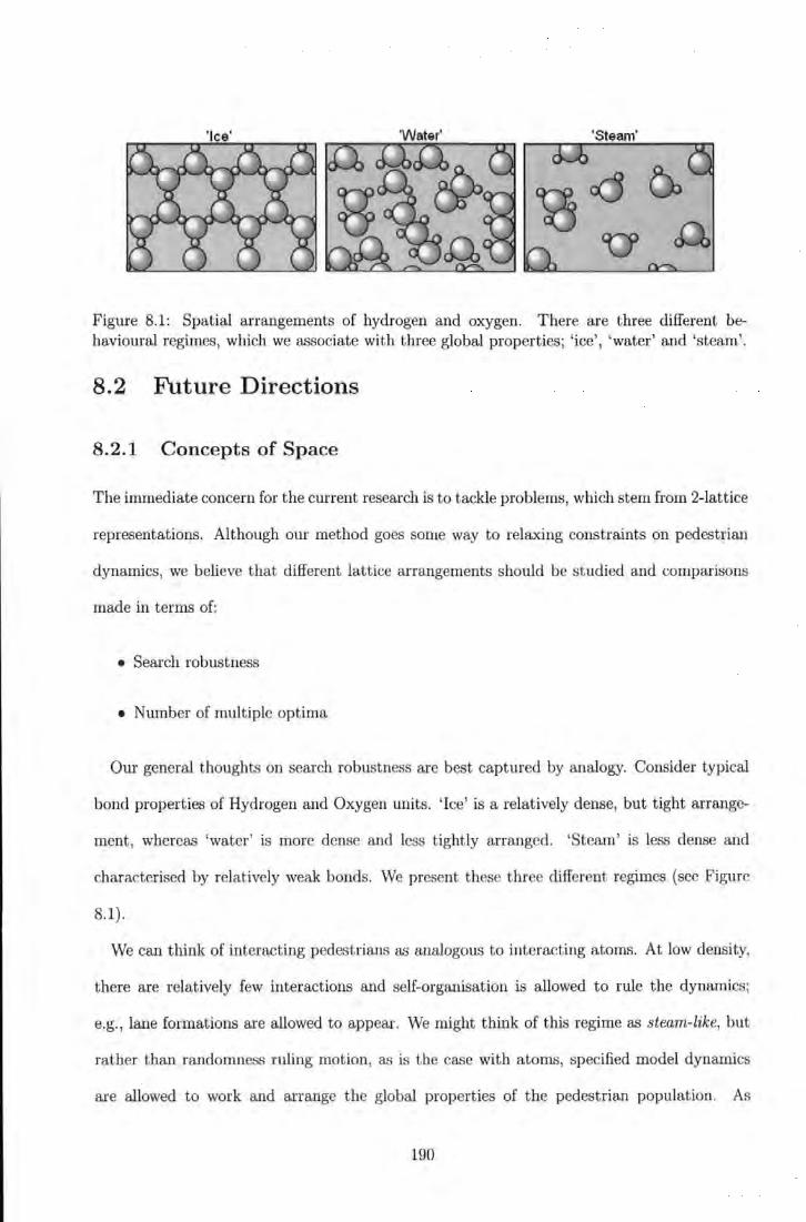
'Steam'

Figure 8.1: Spatial arrangements of hydrogen and oxygen. There are three different behavioural regimes, which we associate with three global properties; 'ice', 'water' and 'steam'.

8.2 Future Directions

8.2.1 Concepts of Space

The immediate concern for the current research is to tackle problems, which stem from 2-lattice

representations. Although our method goes some way to relaxing constraints on pedestrian

dynamics, we believe that different lattice arrangements should be studied and comparisons

made in terms of:

• Search robustness

• Number of multiple optima

Our general thoughts on search robustness are best captured by analogy. Consider typical

bond properties of Hydrogen and Oxygen units. 'Ice' is a relatively dense, but t ight arrange-

ment, whereas 'water' is more dense and less tightly arranged. 'Steam' is less dense and

characterised by relatively weak bonds. We present these three different regimes (see Figure

8.1).

We can think of interacting pedestrians as analogous to interacting atoms. At low density,

there are relatively few interactions and self-organisation is allowed to rule the dynamics;

e.g., lane formations are allowed to appear. We might think of this regime as steam-like, but

rather than randomness ruling motion, as is the case with atoms, specified model dynamics

are allowed to work and arrange the global properties of the pedestrian population. As

190

we increase the density, we reduce the effects of self-organisation. At a critical point we

observe a mixed regime; neither self-organisation or percolation wins. This is water-like;

pedestrian neighbourhoods begin to merge, but not catastrophically, and some of the dynamics

are allowed to unfold between fragmented clusters. Where we increase density above a critical

point, we expect that almost all neighbourhoods connect, where once fragmented clusters now

form a giant-component. This is ice-like; unintended effects in one local region can percolate

far and wide, just like a strong enough force can break hydrogen and oxygen bonds locally,

and weaken the global structure of ice by creating long, percolating cracks.

It is possible that pedestrian models need to move away from square lattice concepts of

space and towards, perhaps, different kinds of lattices. Certainly, a comparison study of

model performance across lattice shapes would be worthwhile. Different vertex connections

could be tested for robustness in the face of increasing density. However, it has been shown

that most different lattices have a lower percolation threshold than the square lattice (Stauffer

and Aharony, 1992). It would, therefore, be unwise to design rule sets on these lattices because

we would expect them to be even less robust.

However, there is one exception, the honeycomb lattice (see Figure 8.2). This lattice has

a percolation threshold Pc ::::: 0.6962, which is approximately 0.1 greater than the threshold

for the von Neurnann lattice. We believe this lattice would be more robust for the design of

pedestrian dynamics. However, we would not claim that the design of appropriate rule sets

for such lattices would be simpler, or even equally as simple, than for more regular lattices.1

In short, if we use discrete spaces, then we need to look towards the design of underlying

representations where percolation thresholds are shifted to much higher densities.

1This is another reason to use an expanding wave approach; it is more computationally expensive than CA rules, but is a general search method, and should be portable to any kind of neighbourhood. At least with this method we could begin to investigate different kinds of lattices without worrying too much about the design of optimal rule sets.

191

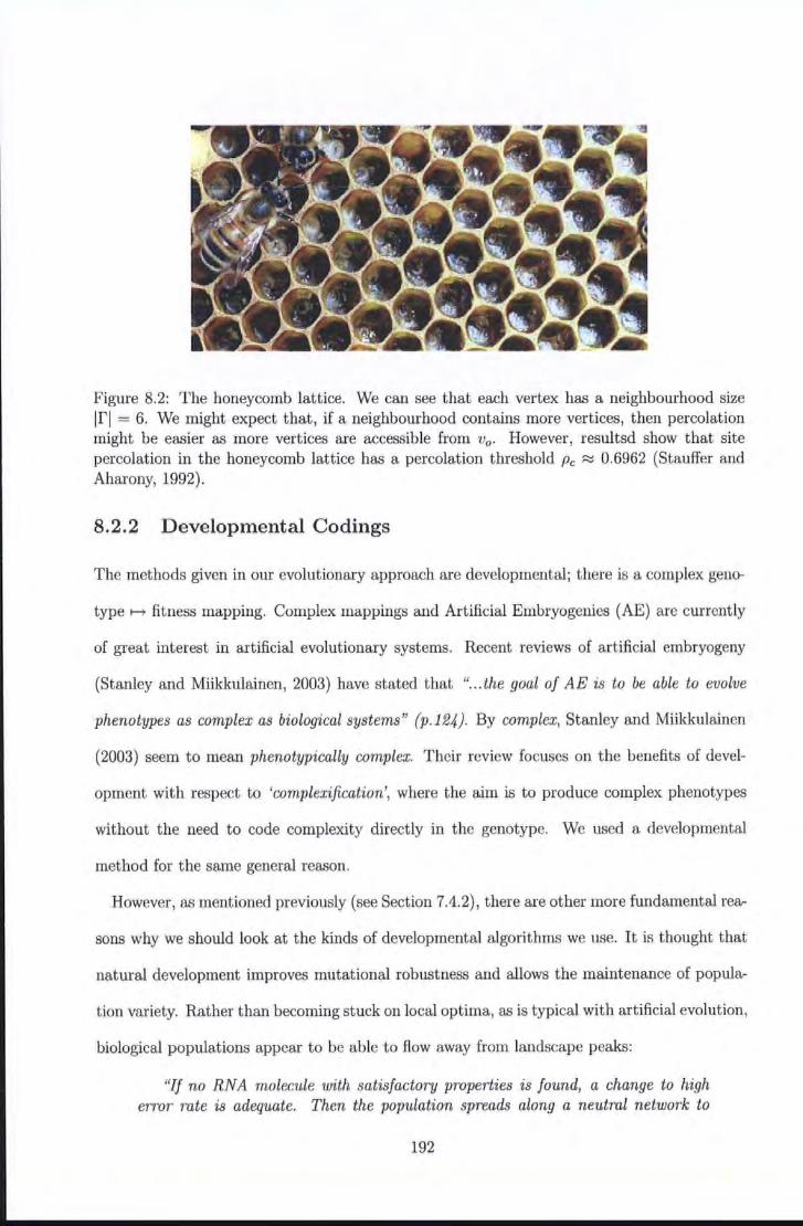
Figure 8.2: The honeycomb lattice. We can see that each vertex has a neighbourhood size If! = 6. We might expect that, if a neighbourhood contains more vertices, then percolation might be easier as more vertices are accessible from v0 • However, resultsd show that site percolation in the honeycomb lattice has a percolation threshold Pc ~ 0.6962 (Stauffer and Aharony, 1992).

8.2.2 Developmental Codings

The methods given in our evolutionary approach are developmental; there is a complex gena-

type t---t fitness mapping. Complex mappings and Artificial Embryogenies (AE) are currently

of great interest in artificial evolutionary systems. Recent reviews of artificial embryogeny

(Stanley and Miikkulainen, 2003) have stated that " ... the goal of AE is to be able to evolve

phenotypes as complex as biological systems" (p.124). By complex, Stanley and Miikkulainen

(2003) seem to mean phenotypically complex. Their review focuses on the benefits of devel-

opment with respect to 'complexification', where the aim is to produce complex phenotypes

without the need to code complexity directly in the genotype. We used a developmental

method for the same general reason.

However, as mentioned previously (see Section 7.4.2), there are other more fundamental rea-

sons why we should look at the kinds of developmental algorithms we use. It is thought that

natural development improves mutational robustness and allows the maintenance of popula-

tion variety. Rather than becoming stuck on local optima, as is typical with artificial evolut ion,

biological populations appear to be able to flow away from landscape peaks:

"If no RNA molecule with satisfactory properties is found, a change to high error rate is adequate. Then the population spreads along a neutral network to

192

other regions in the sequence space, which can be explored in detail after tuning the error rote low again. "

(p 54, Schuster, 1997)

Neutral networks thus connect otherwise fragmented local peaks, allowing populations to

traverse landscapes and converge on successful solutions without sticking to them. In this way,

fault-tolerant development characterises a more open-ended evolutionary search. Recent work

in Artificial Evolution is attempting to harness the properties of these natural landscapes in

order to provide more open-ended mechanisms for artificial adaptation.

Clearly, this kind of research has important implications to the many approaches, which

develop genotypes into phenotypes. It is important to realise that, although developmental

codes provide practical advantages for phenotype creation (Stanley and Miikkulainen, 2003),

these may not necessarily produce fitness landscapes that are easy to traverse. We would

certainly not expect that codes not designed to improve search robustness, in this way, do

so. One aim is therefore to encode developmental mechanisms, which maintain the practi-

ea! advantages, but also allow open-ended evolution. Designing such codes, however, is not

necessarily a trivial task.

8.3 Closing Comments

The aim of this research is to develop useful fitness functions for an Evolutionary approach

to Architectural Design. Thus far, Evolutionary Architecture has been limited by a narrow

vision, where fitness is decided in the context of human decisions about abstract form. We

need to move beyond this approach and incorporate realistic models of important crowd-

How phenomena, which impinge on the design of human-built forms. In this thesis we have

therefore concentrated on developing simple models of complex crowd dynamics.

The usefulness of an evolutionary approach depends very much on the efficacy of these

models, an area where there are challenges still to be met. One of the most important

challenges is perhaps not only in the design of cellular rule sets, but in the development of more

193

•robust cellular spaces: Although we have :demonstnitedi ;the ,usefulness ,of an inclusive search

algmithru for' •produCing ;silnple uiodels of complex !Crowd~ flow" we believe tlut:t sjgllificail.t

:pto~res$ :o11 discr~~e spi,\Ce :caiJ.. only be: m,a.Q~ iil tb.is: dir~cw:m,,

194

Appendix A

Glossary

Autowave the occurrence of internally generated waves, which often depend on local cou-

plings between the excitable units.

Egress the process of movement in a population of pedestrians whose goal is to follow paths

from their current location to exit points of a configuration.

Cellular Automata lattice based rules determined by local-neighbourhood inputs.

Clustering Coefficient a value for the clustering 'Yv = '(1~))1 of a given vertex v, where

IE(fv)l is the degree of v and (k;) is the maximum possible number of simple connections

in rv 1. For a graph G, the clustering coefficient 'Y(G) = 'YvVv E V( G).

Connected Graph the property of a graph G(E, V) where any vertex v; E V is connected

by a walk along edge elements ei E E, such that any other vertex vk E V is accessible

to v;.

Continuous Space a space where coordinates are represented as real, floating point num-

hers.

Degree the number of connections kv protruding from vertex v.

1 By simple we mean bi-directional and, therefore, the maximwn is derived from a binomial distribution.

195

Destination Vertex a vertex vd, which is the last element of a walk away from a vector

origin v0 •

Developmental Algorithm an algorithm, which unfolds over time and often grows in com

plexity. In the context of a genotype ...... phenotype mapping, a compressed genotype

often expands into a more complex phenotype.

Discrete Space a space where vertex coordinates are represented as integer numbers. The

2-lattice is an example of a discrete space.

Dynamic a method which takes as input a given state of a system and then outputs a

different state, based on internal rules.

Field a collection of scalar quantities, which define the global properties of a given space.

These properties are used in evacuation models to define gradients so that pedestrians

can navigate to exit areas.

Fitness Function a general term used for the calculation of fitness for a phenotype. Fitness

is often population-defined in order that individuals can be evaluated against each other.

Fitness functions provide artificial pressures akin to Natural selection.

Genetic Algorithm a nature-inspired algorithm based on Natural Selection. Artificial Dar

winian mechanisms, based on inheritance and mutation, operate on strings of alphabet- -

constrained alleles, which are interpreted in a Genotype ...... Phenotype ...... Fitness map

ping and artificially selected with the use of a fitness function.

Genotype ...... Phenotype ...... Fitness Mapping the rules that define a mapping from a

given Genotype to Phenotype and from a Phenotype to Fitness. The different stages

in this process can be more or less complex depending on the application domain and

nature of problem description.

Graph defined as G(E, V), where E(G) is the edge-set of the graph and V( G) is the vertex

set. Graphs can be single-component or multi-component.

196

Inclusive Search a search where all possible optimal-paths are searched in a link between a

vertex origin V0 and a vertex destination vd.

Lattice a discrete space where vertices are connected by well-defined edge relationships in

simple neighbourhoods. For example, spaces like a 2-lattice can be constructed from

von Neumann neighbourhoods or Moore neighbourhoods.

Local-Global Link v 0 ---> vd the paths (or path) defined between the origin vertex Vo and

the destination vertex vd. The link is derived from a traceback algorithm, applied after

inclusive search.

Mult-Agent System any general system composed of many interacting parts. Such systems

can also been referred to as 'many-particle'.

Multi-Component Graph a graph where a single vertex or cluster is separated from other

clusters in the graph, i.e., the conditions for a connected graph are not met.

Neighbourhood the surrounding of a given vertex v denoted by fv, which may define a

neighbourhood with arbitrary degree k. However, in this thesis immediate neighbour

hoods with degree k = 4 (von Neumann) or k = 8 (Moore neighbourhood) are particu

larly important.

Origin Vertex the vertex v0 currently occupied by a given pedestrian.

Pedestrian and Evacuation Dynamics the ensemble of rules, which determine the state

changes in a given model, designed to represent real pedestrian interactions and evacu

ation processes.

Pedestrian Density p(O, 1) the ratio of occupied lattice vertices to the total amount of

vertices in the lattice.

Percolation the property of diffusion in a spatial system, where diffusive interactions arc

traverse its diameter.

197

Percolation Threshold the point where percolation is first observed in a system.

Pulse Coupled Neural Network a neural network based on a simple spiking neuron model.

This kind of network has been widely used in image processing applications.

Single-Component Graph see 'Connected graph' (above).

Stigmergy the general mechanism of agent-agent interaction, where the spatial environment

is used as a medium of communication.

Vector Canceling the effect of a given procedure where a simple graph, which contains no

directional information, is transformed into one that does, so that field information then

constrains the bi-directionality of edges.

198

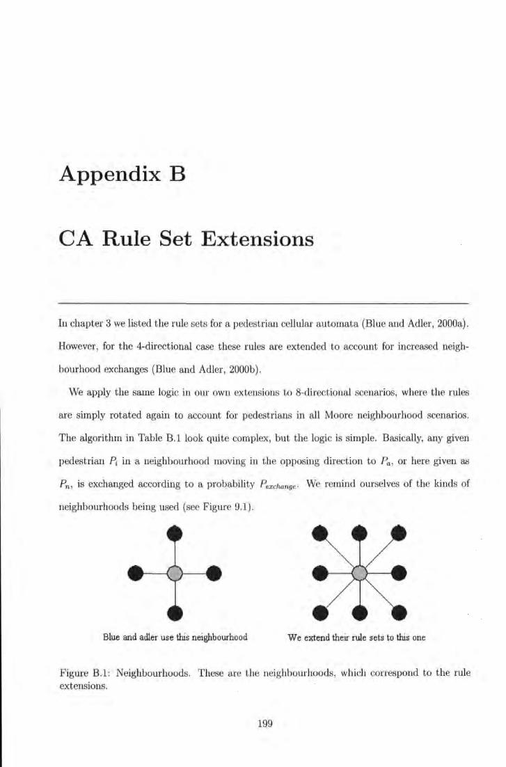
Appendix B

CA Rule Set Extensions

In chapter 3 we listed the rule sets for a pedestrian cellular automata (Blue and Adler, 2000a).

However, for the 4-direct ional case these rules are extended to account for increased neigh-

bourhood exchanges (Blue and Adler , 2000b) .

We apply the same logic in our own extensions to 8-directional scenarios, where the rules

are simply rotated again to account for pedestrians in all Moore neighbourhood scenarios.

The algorithm in Table B.1 look quite complex, but the logic is simple. Basically, any given

pedestrian ~ in a neighbourhood moving in the opposing direction to Pa, or here given as

P n, is exchanged according to a probability P exchange · We remind ourselves of the kinds of

neighbourhoods being used (see Figure 9.1) .

Blue and adler use this neighbourhood We extend their rule sets to this one

Figure B.1: Neighbourhoods. These are the neighbourhoods, which correspond to the rule extensions.

199

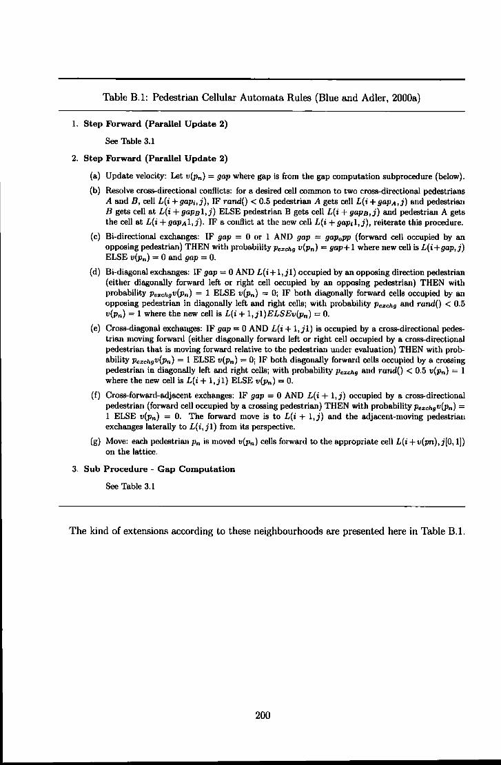
Table B.l: Pedestrian Cellular Automata Rules (Blue and Adler, 2000a}


See Table 3.1


(a) Update velocity: Let v(pn) =gap where gap is from the gap computation subprocedure (below).

(b) Resolve cross-directional conflicts: for a desired cell common to two cross-directional pedestrians A and B, cell L(i+gap;,j), IF rand()< 0.5 pedestrian A gets cell L(i+gapA,j) and pedestrian B gets cell at L(i + gapB1,j) ELSE pedestrian B gets cell L(i + gapB,i) and pedestrian A gets the cell at L(i + gapA1,j). IF a conflict at the new cell L(i + gap1l,j), reiterate this procedure.

(c) Bi-directional exchanges: IF gap = 0 or 1 AND gap = gap0 pp (forward cell occupied by an opposing pedestrian) THEN with probability Pezchg v(pn) = gap+ 1 where new cell is L(i +gap, j) ELSE v(pn) = 0 and gap = 0.

(d) Bi-diagonal exchanges: IF gap = 0 AND L( i + 1, j 1) occupied by an opposing direction pedestrian (either diagonally forward left or right cell occupied by an opposing pedestrian) THEN with probability PezchgV(pn) = 1 ELSE v(pn) = 0; IF both diagonally forward cells occupied by an opposing pedestrian in diagonally left and right cells; with probability Pezchg and rand() < 0.5 v(pn) = 1 where the new cell is L(i + 1,j1)ELSEv(pn) = 0.

(e) Cross-diagonal exchanges: IF gap= 0 AND L(i + 1,j1) is occupied by a cross-directional pedestrian moving forward (either diagonally forward left or right cell occupied by a cross-directional pedestrian that is moving forward relative to the pedestrian under evaluation) THEN with probability Pezchgv(pn) = 1 ELSE v(pn) = 0; IF both diagonally forward cells occupied by a crossing pedestrian in diagonally left and right cells; with probability Pczchg and rand() < 0.5 v(pn) = 1 where the new cell is L(i + 1,j1) ELSE v(pn) = 0.

(f) Cross-forward-adjacent exchanges: IF gap = 0 AND L( i + 1, j) occupied by a cross-directional pedestrian (forward cell occupied by a crossing pedestrian) THEN with probability PezchgV(pn) = 1 ELSE v(pn) = 0. The forward move is to L(i + 1,j) and the adjacent-moving pedestrian exchanges laterally to £( i, j 1) from its perspective.

(g) Move: each pedestrian Pn is moved v(pn) cells forward to the appropriate cell L(i + v(pn),j[O, 1]) on the lattice.

3. Sub Procedure - Gap Computation

See Table 3.1

The kind of extensions according to these neighbourhoods are presented here in Table B.l.

200

Appendix C

Publications

The following publications are included in this order:

Holden, R., and Parmee, I. (2000} Utilising multi-agent based crowd flow models for the evolutionary design of spatial layouts in marine vessels. Proceedings of the 1"1 European Conference on Marine Technology, Nantes, France.

Holden, R., and Cangelosi, A. (2004} Limits to locality in cellular automata models of pedestrian behaviour. Proceedings of Interflam 2004, 101h International Fire Science and Engineering Conference, Edinburgh.

Holden, R., and Cangelosi, A. (2004} A general, computationally intelligent model for egress simulation. Proceedings of Interflam 2004, 101h International Fire Science and Engineering Conference, Edinburgh.

201

Evolutionary Spatial Layout Utilising Agent-Based Models of Crowd Behaviours

Richard Holden' and lan Parmee, Plymouth Engineering Design Centre, University of Plymouth UK.

Abstract

This paJ>er outlines a proposed approach towards gaining useful measures of fitness for architectural spatial layout by utilising a multi - agent based model of crowd behaviour. Issues relating to computer aided design and the biologically inspired techniques that may underpin them in the future are considered. Then the general concept of an agent is outlined both in terms of intrinsic properties and BB a unit within 811 ecological complex. Finally, the future development of the model is related to long term aims of integration within an evolutionary framework.

Introduction

Perhaps one of the most important issues in architectural design is spatial layout. The concept of space is of fundamental importance and this is reftected in architectural theory (Hillier & Hanson 1984). The implication is that spatial configurations can profoundly inftuence the nature of people's movements through space SJld thus certain configurations may be more conducive to the provision of particular movement. A tool capable of providing reliable and useful information on the relationship between spatial layout SJ!d people movemcut may be of great benefit during the process of design.

Inadequate CAD tools

The computer is now an integral part of Architecture courses and just by virtue of its speed the computer is of some use in design. However, it bas beeu pointed out that the use of the phrase Computer Aided Design is more of a misuse because the current software tools do not contribute in any significant way to the octual process of design (.Jackson 1998).

The Architects brain still carries the weight of having to sift through the dizzying amount of information available in order to produce designs that satisfy mSJJY conflicting constraints. Architects will certainly ignore massive spaces of possible designs and many possibly fruitful avenues in completing their design.

• Author to whom c:orrespondence should be addressed: [email protected]

202

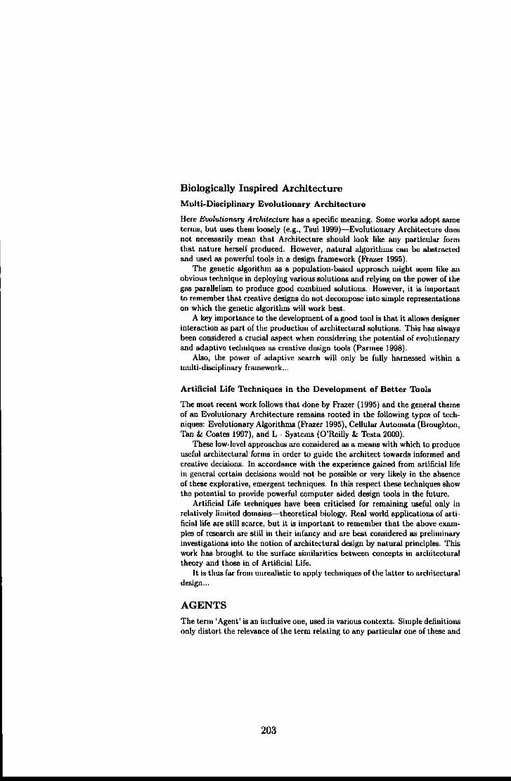
Biologically Inspired Architecture

Multi-Disciplinary Evolutionary Architecture

Here Evolutionary Architecture has a specific meaning. Some works adopt same terlllB, but uses them loosely (e.g., Tsui 1999)-Evolutionary Architecture does not necessarily mean that Architecture should look like any particular form that nature herself produced. However, natural algorithms can be abstracted and used as powerful tools in a design framework (Frazer 1995).

The genetic algorithm as a population-based approach might seem like an obvious technique in deploying various solutions and relying on the power of the gas parallelism to produce good combined solutions. However, it is important to remember that creative designs do not decompose into simple representations on which the genetic algorithm will work best.

A key importance to the development of a good tool is that it allows designer interaction as part of the production of architectural solutions. This has always been considered a crucial aspect when considering the potential of evolutionary and adaptive techniques as creative design tools (Parmee 1998).

Also, the power of adaptive search will only be fully harnessed within a multi-disciplinary framework ...

Artificial Life Techniques in the Development of Better Tools

The most recent work follows that done by Frazer ( 1995) and the general theme of an Evolutionary Architecture remains rooted in the following types of techniques: Evolutionary Algorithms (Frazer 1995), Cellular Automata (Broughton, Tan & Coates 19!17), and L- Systems (O'Reilly & Thsta 2000).

These low-level approaches are considered as a means with which to produce useful architectural forms in order to guide the architect towards informed and creative decisions. In accordance with the experience gained from artificial life in general certain decisions would not be possible or very likely in the absence of these explorative, emergent techniques. In this respect these techniques show the potential to provide powerful computer aided design tools in the future.

Artificial Life techniques have been criticised for remaining useful only in relatively limited domains-theoretical biology. Real world applications of artificial life are still scarce, but it is important to remember that the above examples of research are still in their infancy and are best considered as preliminary investigations into the notion of architectural design by natural principles. This work has brought to the surface similarities between concepts in architectural theory and those in of Artificial Life.

It is thus far from unrealistic to apply techniques of the latter to architectural design ...

AGENTS

The term 'Agent' is an inclusive one, used in various contexts, Simple definitions only distort the relevance of the term relating to any particular one of these and

203

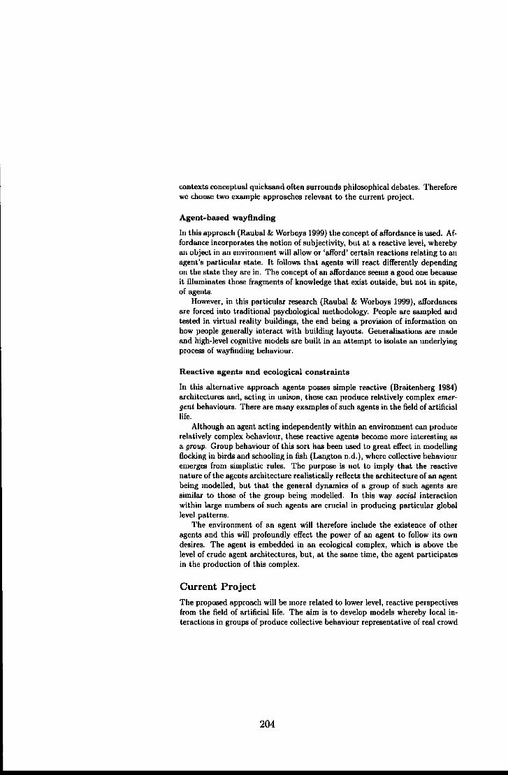
contexts conceptual quicksand often surrounds philosophical debates. Therefore we choose two example approaches relevant to the current project.

Agent-based wayfinding

In this approach (Raubal & Worboys 1999) the concept of affordance is used. Affordance incorporates the notion of subjectivity, but at a reactive level, whereby an object in an environment will allow or 'afford' certain reactions relating to an agent's particular state. It follows that agents will react differently depending on the state they are in. The concept of an affordance seems a good one because it illuminates those fragments of knowledge that exist outside, but not in spite, of agents.

However, in this particular research (Raubal & Worboys 1999), affordances are forced into traditional psychological methodology. People are sampled and tested in virtual reality buildings, the end being a provision of information on how people generally interact with building layouts. Generalisations are made IUld high-level cognitive models are built in an attempt to isolate an underlying process of wayfinding behaviour.

Reactive agents and ecological constraints

In this alternative approach agents posses simple reactive (Braitenberg 1984) architectures and, acting in unison, these can produce relatively complex emergent behaviours. There are many examples of such agents in the field of artificial life.

Although an agent acting independently within an environment can produce relatively complex behaviom, these reactive agents become more interesting as a group. Group behaviour of this sort has been used to great effect in modelling Rocking in birds and schooling in fish (Langton n.d.), where collective behaviour emerges from simplistic rules. The purpose is not to imply that the reactive nature of the agents architecture realistically reRects the architecture of an agent being modelled, but that the general dynamics of a group of such agents are similar to those of the group being modelled. In this way social interaction within large numbers of such agents are crucial in producing particular global level patterns.

The environment of an agent will therefore include the existence of other agents and this will profoundly effect the power of an agent to follow its own desires. The agent is embedded in an ecological complex, which is above the level of crude agent architectures, but, at the same time, the agent participates in the production of this complex.

Current Project

The proposed approach will be more related to lower level, reactive perspectives from the field of artificial life. The aim is to develop models whereby local interactions in groups of produce collective behaviour representative of real crowd

204

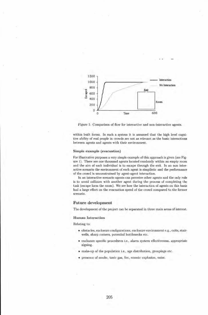
1200

1000 Interaction

No interaction

------800 """ _,..~ Exit " /-g. 600

D~~ 0

~ 400 I I

200 I

0 0 Tune 600

Figure 1: Comparison of Bow for interactive and non-interactive agents.

within built forms. In such a system it is assumed that the high level cognitive ability of real people in crowds are not as relevant as t he basic interactions between agents and agents with their environment.

Simple example (evacuation)

For illustrative purposes a very simple example of this approach is given (see Figure 1). There are one thousand agents located randomly within an empty room and the aim of each individual is to escape through the exit. In an non interactive scenario the environment of each agent is simplistic and the performance of the crowd is unconstrained by agent-agent interaction.

In an interactive scenario agents can perceive other agents and the only rule is to avoid collision with another agent during the process of completing t he task (escape form the room) . We see how the interaction of agents on this basis had a large effect on the evacuation speed of the crowd compared to the former scenario.

Future development

The development of the project can be separated in three main areas of interest .

Human Interaction

Relating to:

• obstacles, enclosure configurations, enclosure environment e.g., exits, stairwells, sharp corners, potential bottlenecks etc.

• enclosure specific procedures i.e., alarm system effectiveness, appropriate signing.

• make-up of the population i.e., age distribution, groupings etc.

• presence of smoke, toxic gas, fire, remote explosion , noise.

205

The Modelling of Interaction

• human-e1aviron1nent interaction

• human-human interaction

• human-hazard interaction

The intention is to initially establish simple behavioural agent-based models that take such interactions into account to some extent. Further development of basic models will rely upon calibration to available data relating to fire evacuation and to passenger evacuation data where available. Development and calibration will continue throughout the duration of the project as further information becomes available and knowledge develops.

It is intended that a degree of machine-learning will be incorporated within the behavioural agent models with a longer term objective of establishing autonomous activity to some extent.

Adaptive Design

The development of an evolutionary/adaptive computing design search, exploration and optimisation framework that utilises the developed behavioural models as objective functions in order to investigate:

• spatial layout i.e., the design of exits, passageways, stairwells, muster points etc.

• positioning of signs and lighting.

• information broadcasting and alarm systems

The emphasis will be upon interactive evolutionary design systems that allow a high degree of user-led exploration of possible scenarios.

References

Braitenberg, V. {1984), Vehicles: Experiments in Synthetic Psychology, Bradford Books, London.

Broughton, T., Tan, A.&. Coates, P. S. {1997), The use of genetic programi.ng in exploring 3D design worlds, in R. Juuge, ed., 'CAAD Futures 97', Kluwer Academic Publishers, Technical University Munich, Germany, pp. 885-917.

Frazer, A. {1995), Evolutionary Architecture, Architectural Association, London.

Hillier, B.&. Hanson, J. {1984), The Social Logic of Space, Cambridge University Press, Cambridge.

206

Jackson, H. (1998), An evolutionary step, Master's thesis, Shoo) of Architecture, University of East London.

Langton (n.d.), Artificial life, chapter 1, pp. 39-94.

O'R.eilly, U. M. & Testa, P. (2000), Representation in architectural design tools, in 'ACDM: proceedings of the conference on adaptive computing iu design and manufacture'.

Parmee, I. (1998), Exploring the design potential of evolutionary/adaptive search and other computational intelligence technologies, in T. Parmec, ed., 'Proceedings of The Third Conference on Adaptive Computing in Design and Manufacture', Springer, London, pp. 27-43.

Raubal, M. & Worhoys, M. (1999), A formal model of the process of wayfinding in built environment, in C. Freksa & D. Mark, eds, 'Spatial Information Theory - Cognitive and Computational Foundations of Geographic lnfor· mation Science', Stade, germany, pp. 381-399.

Tsui, E. (1999), Evolutionary Architecture: Nature as a basis of design, Wiley, New York.

207

Limits To Locality In Cellular Automata Models Of Pedestrian Behaviour

Richard Holden and Angelo Cangelosi Adaptive Behaviour and Cognition Centre for Interactive and Intelligent Systems U Diversity of Plymouth

[email protected]. uk, [email protected]

Abstract

Firstly, we investigate a pedestrian Cellular Automata (CA) model. We show that the model is sensitive to density and seck to control some of the density· dependent randomness in the rule sets, which work against intended pattern formation. The new constraints introduced improve statistical features of the model, but further investigation reveals persistently brittle behaviour. Secondly, we illustrate features of CA spatial representations-interaction properties of the 2-lattice graph. Many models of pedestrian behaviour make implicit use the 2-latticc and we show how this graph determines non-intuitive limits to intended self-organisation. We suggest important implications for local rulebased discrete dynamical models.

1 Introduction

Models of pedestrian movement in discrete spaces have their own domains of application and it is practical to implement specific techniques as needed. However, it is also important that general features of pedestrian behaviour are modelled. In this paper we address CA methods of implementation Rlld their usefulness for modelling the property of lane formation found in crowd populations. CA are iucreRBingly used in this application domain, perhaps due to the success of such kinds of methods in the field of )-dimensional, !-directional car traffic modelling (Nagel & Rasmusscn 1994). However, once a CA rule set moves into a 2-dimensional domain the number of rules needed increRSes and the number of permutations expands significantly.

We introduce tbe connection between a pedestrian CA (Blue & Adler 2000a) and a car CA (Nagel & Rasmussen 1994). Throughout we refer to these models as pedestrian CA and car CA, respectively. We present statistical behaviour of both models and then modify a randomly assigned rule in the pedestrian CA-this rule reinforces mixed lanes and we attempt to conserve the effect of other lane forming rules by constraining its necessarily random nature. Our local constraint controls some of the statistical results, but closer investigation reveals persistent breakdown of self-organised lane formations.

Finally, we present results of Doolean network percolation statistics. We argue that discrete pedestrian models are a specific instance of such networks. We argue that local rule specification is blind to particular effects of density increments-percolation between pedestrian neighbourhoods. We suggest how,

208

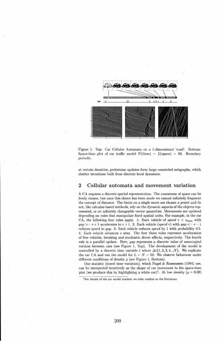
Figure 1: Top: Car Cellular Automata on a 1-dimeusioual ' road'. Bottom: Space-time plot of car t raffic model N(time) = L(space) = 50. Boundary periodic.

at certain densit ies, pedestrian updates form large connected subgraphs, which shat ter intentions built from discrete local dynamics.

2 Cellular automata and movement variation

A CA requires a discrete spatial representation. The coarseness of space can be freely chosen, but once t his choice has been made we cannot infinitely fragment the concept of distance. T he limits on a single move are chosen a priori and do not, like calculus-based methods, rely on the dynamic aspects of the objects represented, or on infinitely changeable vector quantities. Movements are updated depending on rules that manipulate fixed spatial units. For example, in the car CA, the following four rules apply. 1: Each vehicle of speed v < Vma:t with gap>= v + 1 accelerates to v + 1. 2: Each vehicle (speed v ) with gap<= 11 - 1 reduces speed to gap. 3: Each vehicle reduces speed by 1 with probability 0.5. 4: Each vehicle advances v sites. The first three rules represent acceleration of free vehicles, breaking and stochastic driver effects, respectively. The fourth rule is a parallel update. Here, gap represents a discrete value of unoccupied vertices between cars (see Figure 1, Top). The development of the model is controlled by a discrete time variable t where ~t{ 1, 2, 3, 4 ... N}. We replicate the car CA and run the model for L = N = 50. We observe behaviour under different conditions of density p (sec Figure 1, Bottom).

One statistic (travel t ime variation) , which Nagel & Rasmussen (1994) use, can be interpreted int uit ively as the shape of car movement in the space-time plot (we produce this by highlighting a white car)1 . At low density (p = 0.08)

1 For details of the car model statistic we refer readers to the literature.

209

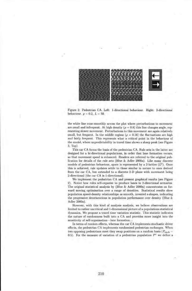
Figure 2: Pedestrian CA. Left: !-directional behaviour. Right : 2-directional behaviour. p = 0.2, L = 50.

the white line runs smoothly across the plot where perturbations to movement are small and infrequent. At high density (p = 0.8) this line changes angle, representing slower movement. Perturbations to this movement are again relatively small, but frequent. In the middle regime (p = 0.16) the fluctuations are h.igh and fairly frequent. This represents what a cri tical point in the behaviour of the model, where uupredictability in travel time shows a sharp peak (see Figure 3, Top) .

This car CA forms the basis of the pedestrian CA. Rule sets in the latter are designed for a bi-directional populations, in order that lane formation occurs, so that movement speed is enbauced. Readers are referred to the original publication for details of the rule sets (Blue & Adler 2000a) . Like many discrete models of pedestrian behaviour, space is represented by a 2-lattice (L2 ) . Once this is achieved, rule updates settle to those similar in nature to ones derived from the car CA, but extended to a discrete 2-D plane with movement being 2-directional (the car CA is !-directional).

We implement the pedestrian CA and present graphical results (see Figure 2). Notice how rules self-organise to produce lanes in 2-directional scenarios. The original statistical analysis by (Blue & Adler 2000a) concentrates on forward moving optimisation over a range of densities. Statistical results show population speed-density relationships as smooth, invested s-shapes, indicating the progressive det.eriorations in population performance over densit.y (Blue & Adler 2000a).

However, with this kind of analysis analysis, we believe observations are limited to rather uncritical and !-dimensional picture of a populations statistical dynamics. We propose a travel time variation statistic. T lus statistic indicates the nature of randomness built into a CA and provides more insight into the sensitivity of self-organisation- lane formation ...

In terms of random effects, whereas the car CA implements stochastic driver effects, the pedestrian CA implements randomised pedestrian exchanges. When two opposing pedestrians meet they swap positions on a random basis ( Pexch = 0.5). For the measure of variation of a pedestrian population p r we define a

210

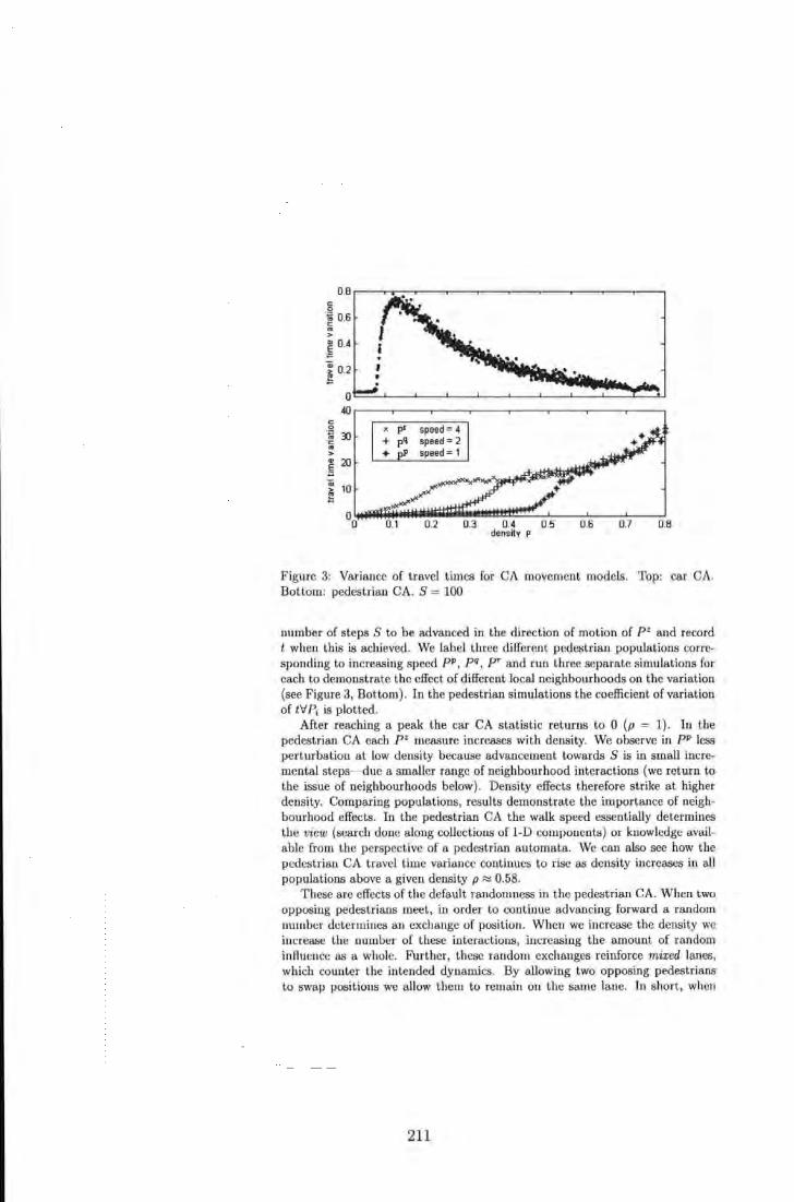
" 0

·~ 0.6 ' C

"' >

~ 0.4

1 0.2 .. oc==-~--~--~--~--~--~--~----L---~~

~-----.----.----.-----.----.----.-----.----,

" 0

·~ )J · ;::

"' >

"' 20 E ·;:; a;

10 ~

Figure 3: Variance of travel times for CA movement models. Top: car CA. Bottom: pedestrian CA. S = 100

number of steps S to be advanced in the direction of motion of P' and record t when this is achieved. We label three different pedestrian populations corresponding to increasing speed PP , pq, p r and run three separate simulations for each to demonstrate t he effect of different local neighbourhoods on the variat ion (see Figure 3, Bot tom) . In the pedestrian simulations the coefficient of variation of tV P; is plotted.

After reaching a peak the car CA statistic returns to 0 (p = 1). In the pedestrian CA each pz measure increases with density. We observe in PP less perturbation at low density because advancement towards S is in small incremental steps- due a smaller range of neighbourhood interactions (we return to the issue of neighbourhoods below). Density effects therefore strike at higher density. Comparing populations, results demonstrate the importance of neighbourhood effects. In the pedestrian CA the walk speed essentially determines the view (search done along collections of 1-D components) or knowledge available from the perspective of a pedestrian automata. We eau also see how the pedestrian CA travel time variance continues to rise as density increases in all populations above a given density p::::: 0.58.

These are effects of the default randomness in the pedestrian CA. When two opposing pedestrians meet, in order to continue advancing forward a random number detenuines an exchange of posit ion. When we increase the density we increase the number of these interactions, increasing the amount of random inAuence as a whole. Further, these random exchanges reinforce mixed lanes, which counter the intended dynamics. By allowing two opposing pedestrians to swap posit ions we allow them to remain on the same lane. In short, when

211

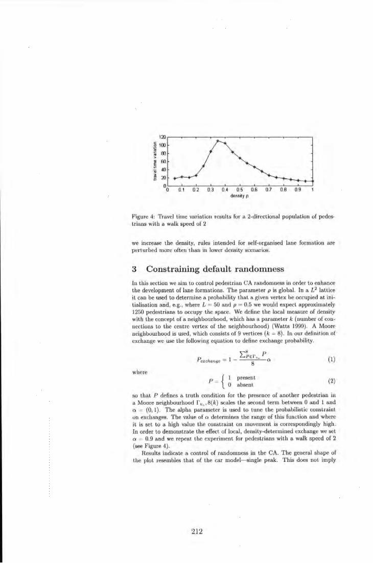
1~.-------.---.---.---.---.---.---.---.---.

.§ 100 .. ':i El) > .. 60

·~ "iii 40

~ ~

0.1 0.2 0.3 0.4 0.5 0.6 0.7 0.6 0.9 density p

Figure 4: Travel time variation results for a 2-direct ional population of pedestrians with a walk speed of 2

we increase the density, rules intended for self-organised lane formation are perturbed more often t han in lower density scenarios.

3 Constraining default randomness

In this section we aim to control pedestrian CA randomness in order to enhance the development of lane formations. The parameter p is global. In a £ 2 lattice it can be used to determine a probability that a given vertex be occupied at initialisation and, e.g., where L = 50 and p = 0.5 we would expect approximately 1250 pedestrians to occupy the space. We define the local measure of density with the concept of a neighbourhood, which has a parameter k {number of connections to the centre vertex of the neighbourhood} (Watts 1999}. A Moore neighbourhood is used, which consists of 9 vertices (k = 8}. In our definition of exchange we use the following equation to define exchange probability.

L~Er •• P P erchange = 1 -

8 er {1}

where p _ { 1 present

- 0 absent {2}

so that P defines a truth condition for the presence of another pedestrian in a Moo re neighbourhood r v., 8{ k) scales the second term between 0 and 1 and er = {0, 1}. The alpha parameter is used to tune the probabilistic constraint on exchanges. The value of er determines the range of this function and where it is set to a high value the constraint on movement is correspondingly high. In order to demonstrate the effect of local, density-determined exchange we set er = 0.9 and we repeat the experiment for pedestrians with a walk speed of 2 (see Figure 4).

Results indicate a control of randomness in the CA. T he general shape of the plot resembles that of the car model-single peak. This does not imply

212

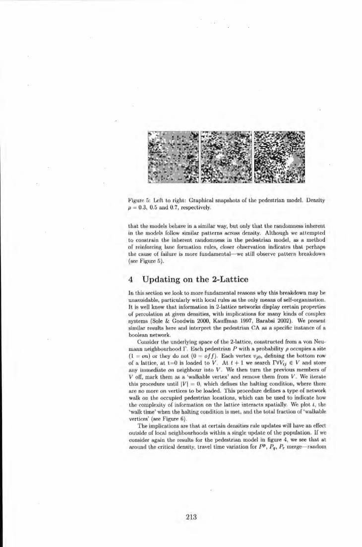
Figure 5: Left to right: Graphical snapshots of the pedestrian model. Density p = 0.3, 0.5 and 0.7, respectively.

that t he models behave in a similar way, but only that the randomness inherent in the models foUow similar patterns across density. Although we attempted to constrain the inherent randomness in the pedestrian model, as a method of reinforcing lane formation rules, closer observation indicates that perhaps the cause of failure is more fundamental-we still observe pattern breakdown (see Figure 5).

4 Updating on the 2-Lattice

In this section we look to more fundamental reasons why this breakdown may be w1avoidable, particularly with local rules as the only means of self-organisation. It is weU know that information in 2-lattice networks display certain properties of percolation at given densities, with implications for many kinds of complex systems (Sole & Goodwin 2000, Kauffman 1997, Barabsi 2002). We present similar results here and interpret the pedestrian CA as a specific instance of a boolean network.

Consider the underlying space of the 2-lattice, constructed from a von Neumann neighbourhood r . Each pedestrian P with a probability p occupies a site (1 = on) or they do not (0 = of f). Each vertex Vjo, defining the bottom row of a lattice, at t= O is loaded to V . At t + 1 we search f\IV;i E V and store any immediate on. neighbour into V . We then turn the previous members of V off, mark them as a 'walkable vertex' and remove them from V . We iterate this procedure until lVI = 0, which defines the halt ing condition, where there are no more on vertices to be loaded. This procedure defines a type of network walk on the occupied pedestrian locations, which can be used to indicate how the complexity of information on the lattice interacts spatially. We plot t , the 'walk t ime' when t he halting condition is met, and the total fract ion of 'walkable vertices' (see Figure 6) .

The implications are that at certain densities rule updates will have an effect outside of local neighbourhoods within a single update of the population. lf we consider again the results for the pedestrian model in figure 4, we see that at around the critical density, travel time variation for pP, Pq, Pr merge-random

213

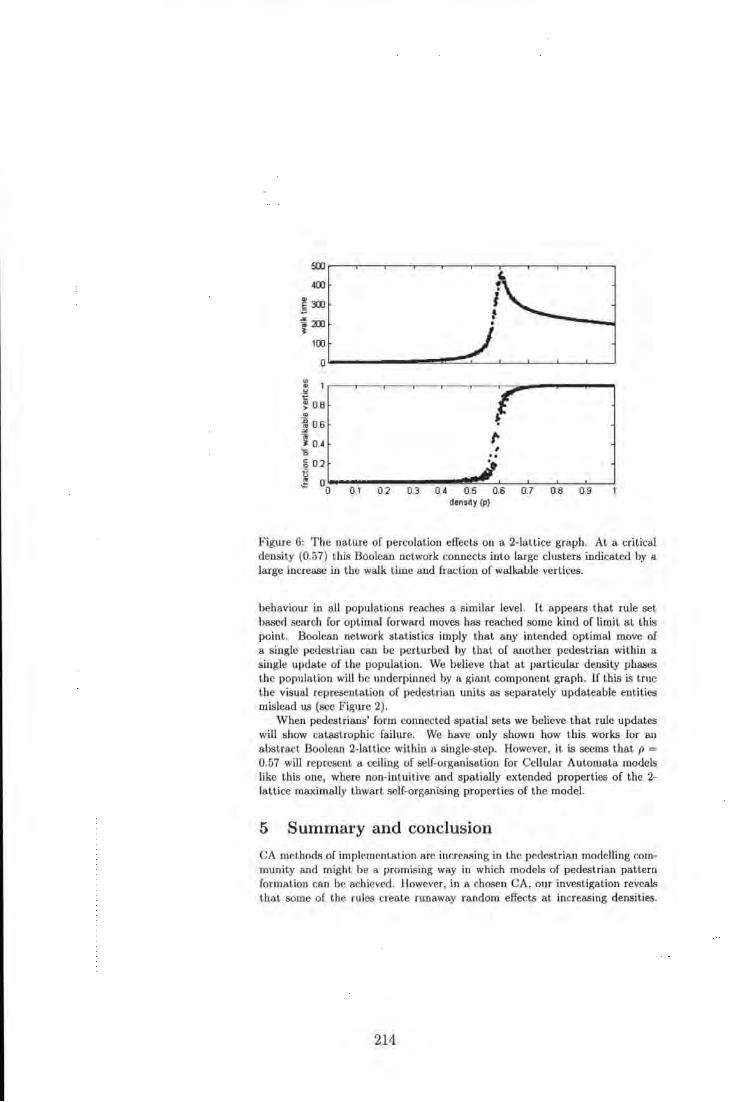
~r---.-~--~---.---,---,---.---.---.--~

400

eDJ ·;:;

.. .. u ·,;:

100

: 0.8 .. ~ 0.6 .><

l 0.4 '15

~ /" , .. ... a o.2

•t; ~ 00*-----------------~~L---L---L-~--_j

0.1 0.2 0.3 0.4 0.5 0.6 0.7 0.8 0.9 density (p)

Figure 6: T he nature of percolation effects on a 2-lattice graph. At a critical density (0.57) this Doolean network connects into large clusters indicated by a large increase in the walk time and fraction of walkable vertices.

behaviour in all populations reaches a similar level. It appears that rule set based search for optimal forward moves has reached some kind of limit at this point . Boolean network statistics imply that any intended optimal move of a single pedestrian can be pertmbed by that of another pedestrian within a single update of the population. We believe that at particular density phases the population will be underpinned by a giant component graph. If this is true t he visual representation of pedestrian units as separately updateable entities mislead us (sec Figme 2) .

When pedestrians' form connected spatial sets we believe that rule updates will show catastrophic failme. We have only shown how this works for an abstract Boolean 2-lattice within a single-step. However, it is seems that p = 0.57 will represent a ceiling of self-organisation for Cellular Automata models like this one, where non-int ui tive and spatially extended propert ies of the 2-la ttice maximally thwart self-organising properties of the model.

5 Summary and conclusion

CA methods of implementation are increasing in the pedestrian modelling community and might be a promising way in which models of pedestrian pattern formation can be achieved. However, in a chosen CA, our investigation reveals that some of the rules create runaway random effects at increasing densities.

214

One plausible approach to remedy this is to attempt to control this randomness at its source, locally from within the rule sets. On closer inspection, however, pedestrian CA statistics are shown to hide what appear to be catastrophic failures in self-<lrganisation, indicating that other less apparent dynamic mechanism are running the show, rather than the discrete dynamic rules by design.

We have suggested that the problem could lie in the localisation of rule design in these models. As an instance of a Boolean 2-lattice, the presence of certain quantities of other pedestrians can seriously undermine the knowledge gained from a local neighbourhood. Although vertices are discrete entities, neighbourhoods are not. Changes in one neighbourhood can have effects that percolate outside a given local region. These kinds of behaviours have been known in the field of computational physics and graph theory for some time. The notion of percolation is important for CA modelB of pedestrian pattern formation because many CA models rely on a graph representation of space.

In short, to maintain pedestrian patterns across the entire density range, it seems that discrete pedestrian models might be forced to use higher-level search algorithiiiS in the face of limits to locality.

References

Barabsi, A. {2002), Linked: The New Science of Networks, Perscus Publishing, Cambridge.

Blue, V. & Adler, J. (2000a), Cellular automata model of emergent collective bi-directional pedestrian dynamics, in 'Artificial Life VII', pp. 437-445.

Kauffman, S. (1997), The Origins of Order: Self-Organi8ation and Selection in Evolution, Oxford University Press, New York.

Nagel, K. & Rasmussen, S. (1994), Traffic at the edge of chaos, in 'Artificial Life IV: Proceedings of the Fourth International Workshop on the Synthesis and Simulation of Living SysteiDB'.

Sole, R. & Goodwin, B. (2000), Signs of Life: How complexity pervades biology, Basic Books, New York.

Watts, D. (1999), Small Worlds: The Dynamics of Networks Between Order and Randomness, Princeton Studies in the Science of Complexity, Princeton.

215

A General, Computationally Intelligent Model of Egress Behaviour

Richard Holden and Angelo Cangelosi Adaptive Behaviour and Cognition Centre for Interactive and Intelligent Systems University of Plymouth

[email protected]. uk, [email protected]. uk

Abstract

We present statistical features of a 2-lattice graph and argue that a search alg<r rithm for pedestrian movement will need to cope with network-level information. As a candidate search algorithm, we introduce a Pulse Coupled Neural Network (PCNN). We improve the search mechanisms in the PCNN equations and show how it can then be used as a general search algorithm for pedestrian models. We present results, which demonstrate the search capacity of these networks in pedestrian occupied spaces. Two discrete-dynamic models are then outlinedpedestrian lane formation and pedestrian egress. Lane formation results are presented and compared to a Cellular Automaton (CA) model. Results show bow the network approach is more robust in high-density situations. Egress and exit choices show the potential generality of the approach. We discuss the potential of our technique as a general method for egress model specification for use within the pedestrian and evacuation modelling community.

1 Introduction

The field of pedestrian modelling contains numerous approaches to rule specification. Some models use global information in the form of potential fields to help specify rules of movement (Owen, Galea & Lawrence 1996), whereas others use local rule-sets in order to produce emergent patterns (Blue & Adler 2000a) . We have argued elsewhere that the latter is an interesting, but fundamentally limited technique (Holden & Cangelosi 2004). ln this paper we are concerned with investigating a new approach to emergent patterns. However, instead of relying on purely local rules we argue that a higher-level network search is necessary in order to provide sufficient information for pedestrians to navigate effectively in complex environments.

We present graphical results of information percolation on a type of 2-lattice graph. The reason we look towards a network approach is related to the effects identified on the 2-lattice. If effects can percolate outside of a given neighbourhood, then it would be a useful approach to search for optimal moves at the level of this information, rather than according to fixed rule sets and limited neighbourhood sizes, as is common in Cellular Automata approaches (Blue & Adler 2000a). We believe that a network-based approach to modelling pedestrian behaviour may be more robust to density parameters. The Pulse Coupled Neural Network (PCNN) is a candidate network approach, identified previously

216

as a possible search engine for complex maze solutions (Caulfield & Kinaer 1999). We investigate the usefulness of tbe PCNN in the domain of pedestrian modelling. We preaent equations of artificial neuron units and demonstrate bow theae units behave in 1 and 2-lattice arrays. A natural property of theae networks is the production of autowaves. We preaent equations that can enhance autowave properties before going ou to demonstrate how theae networks can produce optimal path information in an occupied configuration. However, as results of 2-lattice percolation indicate, search becomes suddenly constrained at critical density values and we identify situations where redundancy in tbe search algorithm peaks. We then alleviate these effects by encoding directional information to the network, which produces lane formation effects in a given experimental set-up. We compare results with a Cellular Automaton (Blue & Adler 2000a). Finally, we demonstrate the generality of our approach by testing it in an 'exit choice' configuration, initialised with directional populations. We discuss results and intended future directions.

2 Properties of a 2-Lattice (k = 8)

Properties of Boolean information on a 2-lattice graph are well known (critical behaviour, percolation, fractal properties) and results relating to connectivity have implications for many complex systems (Sole & Goodwin 2000). We have suggested that the reason for catastrophic breakdown of local rule set approaches, such as CA, is because of emerging, giant component sub-networks of pedestrians, which thwart the intended effects of local updates (Holden & Cangelosi 2004). We preaent behaviour for a 2-lattice with Moore (k = 8) neighbourhoods (see Figure 1). We observe the critical range to be around 4.1, where the walk length and the fraction of walkable sites show large increases 1

.

3 Pulse Coupled Neural Network (PCNN)

The PCNN is a variation of a particular model of the visual cortex. It was originally intended for use in image pre-procesaing tasks, but has also been applied to a number of other application domains (Caulfield & Kinaer 1999, Lindblad & Kinser 1998). The model for a single neuron contains five basic compartments, described by the following equations:

1 More det.a.iled explanations exist in the liU.erBLurc (Sole & Goodwin 2000, Holden k Cangelosi 2004)

217

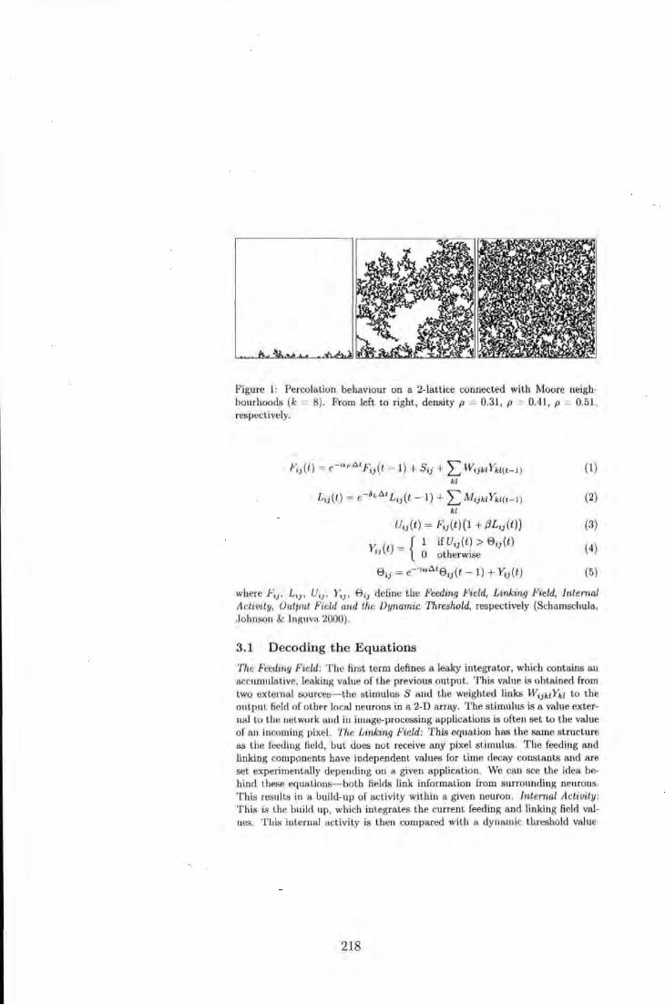
Figure 1: Percolation behaviour on a 2-lattice connected with Moore neighbourhoods (k = 8). From left to right, density p = 0.31, p = 0.41, p = 0.51 , respectively.

fi;(l) = e-oFAtF;;(l-l) + S;; + 2:.: W;jktYkt(t - 1)

kl

L;;(l) = e-6Lt>.t£;1(t- 1) + 2:.: M ;jktYkt(t - 1)

kl

U;;(t) = F1;(t}(l + jJL,1(t))

Y.· (t) = { 1 if U;1(t) > 8;1(t) '1 0 otherwise

8;; = e_..,9 618 ;1(t - 1) + Y;1(t )

(I)

(2)

(3)

(4)

(5)

where F;1, L;;, U,; , Y;;, 8;; define the Feeding Field, Linking Field, Internal Activity, Output Field a11d the Dynamic Threshold, respectively (Schamschula, Johnson & lnguva 2000).

3.1 Decoding the Equations

The Feeding Field: T he first term defines a leaky integrator, which contains au accumulative, leaking value of the previous output. This value is obtained from two external sources-the stimulus S ru1d the weighted links W ;jkl Ykt to the output field of other local neurons in a 2-D array. The stimulus is a value external to the network and iu image-processing applications is often set to the value of an incoming pixel. The Link:ing Field: This equation has the same structure as the feeding field, but does not receive auy pixel stiwulus. The feeding and linking components have independent values for time decay constants and are set experimentally depending on a given application. We can see the idea behind these equations- both fields link information from surrounding neurons. This results in a build-up of activity within a given neuron. Internal Activity: T his is the build up, which integrates the current feeding and linking field values. This internal activity is then compared with a dynamic threshold value.

218

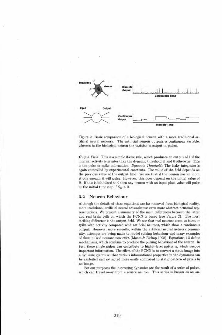
Input Output

Figure 2: Basic comparison of a biological neuron with a more traditional artificial neural network. The artificial neuron outputs a continuous variable, whereas in the biological neuron the variable is output in pulses.

Output Field: This is a simple if-else rule, which produces an output of 1 if the internal activity is greater than the dynamic threshold e and 0 otherwise. Tllis is the pulse or spike information. Dynamic Threshold: The leaky integrator is again controlled by experimental constants. The value of the field depends ou the previous value of the output field. We see that if the neuron has an input strong enough it will pulse. However, this does depend on the initial value of 8 . If this is initialised to 0 then any neuron with an input pixel value will pulse at the iuitial t ime step if S;; > 0.

3.2 Neuron Behaviour

Although the details of these equations are far removed from biological reality, more t raditional artificial neural networks use even more abstract neuronal representations. We present a. summary of the main differences between the latter and real brain cells on which the PCNN is based (see Figure 2). T he most striking difference is the output field. We see that real neurons seem to burst or spike with activity compared with artificial neurons, which show a continuous output. However, more recently, within the artificial neural network community, attempts are being made to model spiking behaviour and many examples of these pulsed neurons now exist {Maass & Bishop 1998). Equations 1-5 define mechanisms, which combine to produce the pulsing behaviour of the neuron. In turu these single pulses can contribute to higher-level patterns, which encode important information. The effect of the PCNN is to convert a static image into a dynamic system so that various informational properties in the dynamics can be exploited and extracted more easily compared to static pattern of pixels in an image.

For our purposes the interesting dynamics are the result of a series of pulses, which can travel away from a source neuron. This series is known as an au-

219

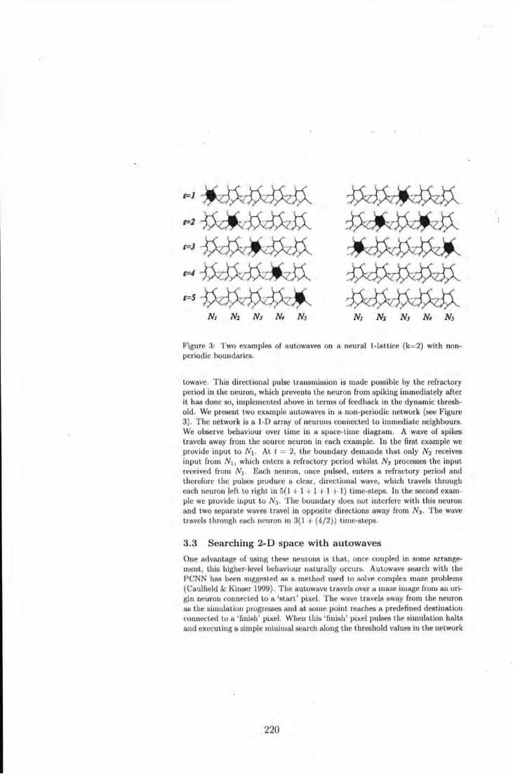
t=l~ t=2~

t=3~

t=4~ t=S~

Figure 3: Two examples of autowaves on a neural 1-lattice (k=2) with nonperiodic boundaries.

towave. This directional pulse transmission is made possible by the refractory period in the neuron, which prevents the neuron from spiking immediately after it has done so, implemented above in terms of feedback in the dynamic threshold. We present two example autowaves in a non-periodic network (see Figure 3). The network is a. 1-D array of neurons connected to immediate neighbours. We observe behaviour over time in a space-time diagram. A wave of spikes travels away from the source neuron in each example. In t he first example we provide input to N1 . At t = 2, the boundary demands that only N2 receives input from N 1, which enters a refractory period whilst N2 processes the input received from N1• Each neuron, once pulsed, enters a refractory period and therefore the pulses produce a clear, directional wave, which travels through each neuron left to right in 5( 1 + 1 + 1 + 1 + 1) lime-steps. In the second example we provide input to N3 . The boundary does not interfere with tllis neuron and two separate waves travel in opposite directions away from N3. The wave travels through each neuron in 3(1 + (4/2)) time-steps.

3.3 Searching 2-D space with a utowaves

One advantage of using these neurons is that, once coupled in some arrangement, this higher-level behaviour natura.lly occurs. Autowave search witll the PCNN has been suggested as a method used to solve complex maze problems (Cauliield & Kiuser 1999). The autowave t ravels over a maze image from an origin neuron connected to a 'start' pixel. The wave travels away from the neuron as the simulation progresses and a t some point reaches a predefined destination connected to a 'finish' pixel. When this 'finish ' pixel pulses the simulation halts and executing a. simple minimal search along the t hreshold values in the network

220

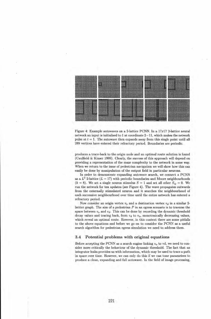
Figure 4: Example autowaves on a 2-lattice PCNN. In a 17x17 2-lattice neural network an input is initialised to 1 at coordinate 2-11, which makes t he network pulse at l = 1. The autowave then expands away from this single point until all 289 vertices have entered their refractory period. Boundaries are periodic.

produces a trace-back to the origin node and an optimal route solution is found (Caulfield & Kinser 1999). Clearly, the success of this approach will depend on providing a representation of the maze complexity to the network in some way. When we return to the issue of pedestrian navigation we will show how this can easily be done by manipulation of the output field in particular neurons.

In order to demonstrate expanding autowave search, we connect a PCNN as a £ 2 2-lattice (L = 17) with periodic boundaries and Moore neighbourhoods (k = 8). We set a single neuron stimulus S = 1 and set all other S;j = 0. We run the network for ten updates (see Figure 4). The wave propagates outwards from the externally stimulated neuron and it searches the neighbourhood of each successive neighbourhood over time until the entire network has entered a refractory period.

Now consider an origin vertex V0 and a destination vertex Vd in a similar 2-lattice graph. The aim of a pedestrian P in an egress scenario is to traverse the space between V 0 and Vd· This can be done by recording the dynamic threshold decay values and tracing back, from Vd to v0 , monotonically decreasing values, which reveal an optimal route. However, in this context there are some pitfalls to the above equations and before we go on to consider the PCNN as a useful search algorithm for pedestrian egress simulation we need to address them.

3.4 Potential problems with original equations

Before accepting the PCNN as a search engine linking V0 to vd, we need to consider more critically the behaviour of the dynamic threshold. T he fact that an integrator leaks provides us with information, which may be used to trace a path in space over time. However, we can only do this if we can tune parameters to produce a clean, expanding and full autowave. In the field of image processing,

221

autowaves from clear images do seem to produce clean autowaves, but depending on the parameters and communication between neurons, wave features may fragment (Lindblad & Kinser 1998). The threshold function, therefore, might potentially produce missing pieces of information. We need to be careful bow we set parameters. Three scenarios are possible. I) In the case where a clean and full autowave expanda from v0 to Vd, the function will be a simple, unperturbed decay shape and we will be able to uncover a link between V0 and tld- 2) If the time decay constants are too strong, then the wave may not reach Vd, because it essentially rullS out of energy. In this case, only temporal information is provided, which is the same in all directions and so there is no direction or specific trace back possible. 3) If we set parameters that allow a neuron to pulse more than once before the wave front hits vd, local optima in the network can result. Scenario I is desirable, whereas scenarios 2 and 3 are undesirable. In order to ensure the first scenario we enhance the autowave features by pruning some of the pulse-recruitment mechanisms in the original equatiollS:

L;j(t) = e-6L"'' L;;(t- I)+ L M;jkl Ykl(t-1) kl

U;J(t) = F;J -1- L;J

ifU;j(l) > 8;j(l) otherwise

(6)

(7)

(8)

(9)

(10)

where, again, F;j, L;j, U;j. Y;j, 8;j define the Feeding Field, Linking Field, lntenaal Activity, Output Field and the Dynamic Threshold, respectively.

There are three main changes in the new PCNN equatiollS. ~'irstly, in the image processing application, F;j sums links to neighbouring neurons with S. Here we only use S. We do this because S can be used to identify the pedestrian location V0 on a 2-D plane and itself produce the start of an autowave. The effect of equation I is to encourage local pulsing through feedback, which as we have explained is undesirable. The corresponding equation, equation 6, relies only on external stimulm. In addition, by turning off the stimulus as soon as a neuron pulses, we ensure that all information used in the threshold comes from the linking field only, reducing feedback and the tendency of neurons to recruit each other to fire. This reduces the problem of multiple pulses and the creation of local optima because there is less information being input to the neuron. Secondly, instead of U;; being a non-linear combination as in equation 6.3, it is now the sum of the feeding and linking fielda. Finally, we introduce a new term in the dynamic threshold, where V" is a large amplification factor. This COIIStant provides a me8118 to ensure that the threshold value is very high, with the effect of extending the period of refraction in a neuron. Settiug this constant to a large value allows the wave to remain directional because multiple pulses should not occur at a single neuron site. We present a schematic for the

222

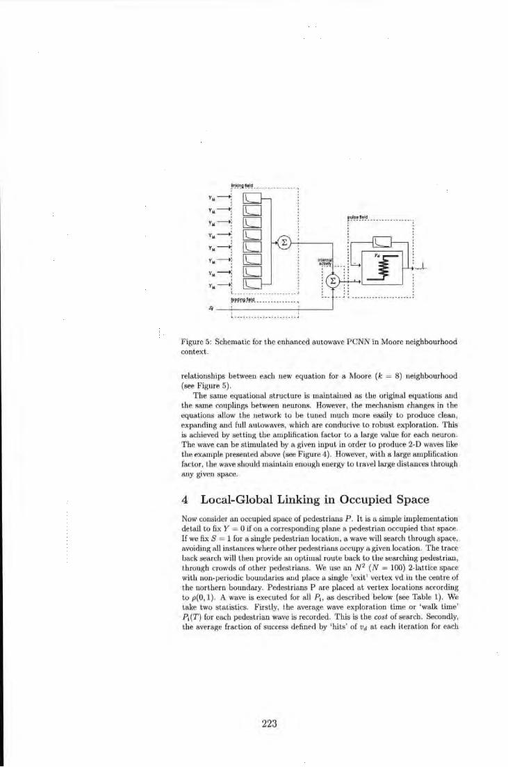
!!'!"!~ii~·J~- - - ------------

Yw~

yl4-+:

ylli-----+: Yw~

~~~~~!~------- ------- -·:

Internal Yid -+: '

yld -+:

!mp· !. ·~---· - '......L

y._ -----.:

L- .• - - - . ·---- •·- .•••••• .J

~~~1!>9-~ld ___ -- -- ---- - -- -, s, _ __._ _______ ~---'

: i L ••• ·· · · ·••· · •·. · · · • • · · .J

Figure 5: Schematic for the enhanced autowave PCNN in Moore neighbourhood context.

relationships between each new equation for a Moore (k = 8) neighbourhood (see Figure 5).

The same equatioual structure is maintained as the original equations and the same couplings between neurons. However, the mechanism changes in the equations allow the network to be tuned much more easily to produce clean, expanding and full autowaves, which are conducive to robust exploration. This is achieved by setting the amplification factor to a large value for each neuron. The wave can be stimulated by a given input in order to produce 2-D waves like the example preseuted above (see Figure 4). However, with a large amplification factor, the wave should maintain enough energy to travel large distances through any given space.

4 Local-Global Linking in Occupied Space

Now consider an occupied space of pedestrians P. It is a simple i1uplernentation detail to fix Y = 0 if on a corresponding plane a pedestrian occupied that space. If we fix S = 1 for a single pedestrian location, a wave will search through space, avoiding all instances where other pedestrians occupy a given location. The trace back search will then provide an optimal route back to the searching pedestrian, through crowds of other pedestrians. We use an N 2 (N = 100) 2-lattice space with non-periodic boundaries and place a single 'exit ' vertex vd in t he centre of the northern boundary. Pedestrians P are placed at vertex locations according to p(O, 1). A wave is executed for all P;, as described below (see Table 1). We take two statistics. Firstly, t he average wave exploration time or 'walk time' P;(T) for each pedestrian wave is recorded. This is the cost of search. Secondly, the average fraction of success defined by 'hits' of Vd at each iteration for each

223

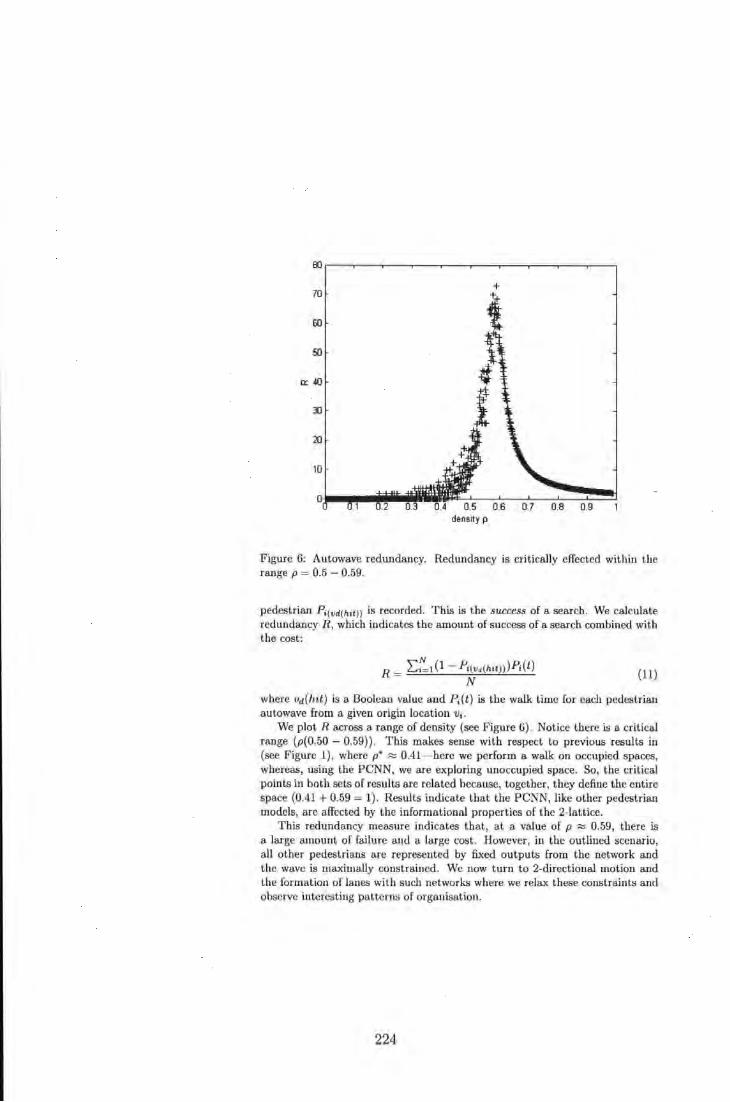
70

60

50

a::40

20

10

0.6 0.7 0.8 0.9 dens~y p

Figure G: Autowave redundancy. Redundancy is critically effected within the range p = 0.5 - 0.59.

pedestrian P;(ud(hit)) is recorded. This is the success of a search. We calculate redundancy R, which indicates t he amount of success of a search combined with t he cost:

R = 2:::: 1 (1 - P;(w(hit)J )P; ( l )

N (11)

where vd(hit ) is a Boolean value and P;(t) is the walk t ime for each pedestrian autowave from a given origin location v1•

We plot R across a range of density (see Figure G). Notice there is a critical range (p(0.50- 0.59)). This makes sense with respect to previous results in (see Figure 1), where p• ::::: 0.41- here we perform a walk on occupied spaces, whereas, using the PCNN, we are exploring unoccupied space. So, the critical points in both sets of results are related because, together, they define the entire space (0.41 + 0.59 = 1). Results indicate that the PCNN, like other pedestrian models, are affected by the informational properties of the 2-lattice.

This redundancy measure indicates that, at a value of p ::::: 0.59, there is a large amount of failure and a large cost . However, in the outlined scenario, all other pedestrians a re represented by fixed outputs from the network and the wave is maxima.Uy constrained. We now turn to 2-directional motion and the formation of lanes with such networks where we relax t hese constraints and observe interesting patterns of organisation.

224

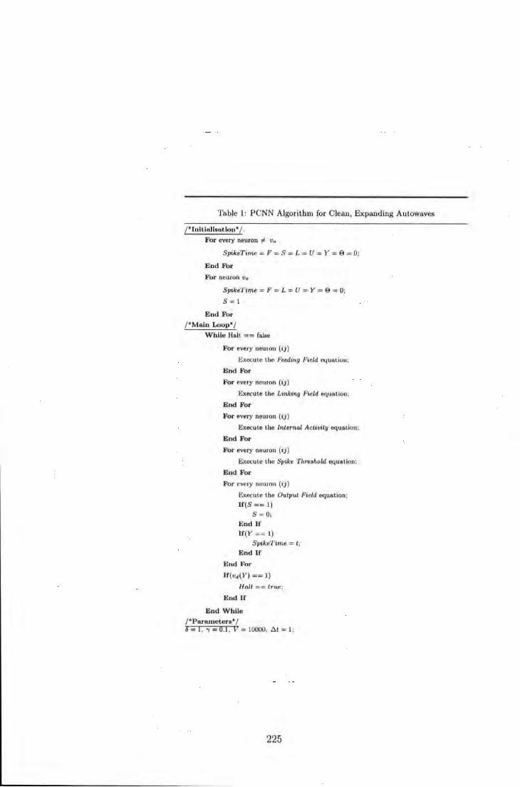
Table 1: P CNN Algorithm for Clean, Expanding Aut.owaves

/*Initialisation*/

For every neuron # Vo

SpikeTime = F = S = L = U = Y = 8 = 0;

End For

For neu.ron Vo

SpikeTime = F = L = U = Y = 8 = 0;

8=1

End For

/*Main Loop*/

While Halt == false


Execute the Feeding Field equation;

End For


Execute the Linking Field equation;

End For


Execute the lnte"'al Activity equation;

End For


Execute the Spike 'Threshold equation;

End For


Execute the Output Field equation;

lf(S ==I)

8 = 0; End If

If(Y == 1) SpikeTime = t ;

End If

End For

If(vd(Y) == I)

Halt == !rue;

End If

End While

r Parameters*/ o- 1, "' - 0.1 , V= 10000, At= I ;

225

5 Pedestrian Interaction Model of Lane Formation

Lane formation behaviour is very important in optimising forward movement in crowds (Blue & Adler 2000a, Hclbing, Farkas & Vicsek 2000). In order to test the lane formation ability of our model, it is important to provide each pedestrian with knowledge of the movement of surrounding pedestrians. Above we outlined an approach for representing the positions of other agents by fixing Y = 0. However, we did not consider here factors relating to the directions of movement. In other models, directional movement is achieved by, for example, introducing a relaxation term to a vector in continuous space (Helbing et al. 2000) or by labelling each pedestrian and creating rules around these labels in discrete space (Diue & Adler 2000a). In our model, a discrete model, we also label our pedestrians and then use this label to determine how pedestrians are accounted for in terms of their relative direction of motion. The assumption behind our approach reAects an idea that pedestrians moving in the same direction physically interact less than with those moving in the opposite direction.

We define a population of pedestrians p•, sub-divided into two populations P" and P'. We define the immediate neighbourhood r(vo);lfP' and fix Y = 0 If p• in this neighbourhood so that each pedestrian has knowledge of the occupancy of all other pedestrians in its immediate surroundings. Outside of this neighbourhood we only apply inputs f"'Pl'(n,•l, so that each pedestrian only has a knowledge of pedestrians with the opposite sign. We define Vd as V 0 +M, where M is a positive value defined relative to the movement direction. At each time-step each pedestrian makes a move towards Vd, so that it continually moves forward in the direction of motion. For a 2-lattice (N2 ), in order to present quantitative results for lane formation behaviour, we use the following to calculate the amount of pedestrian homogeneity I in a given lane i:

I;= max(P",P'); max(P", P•); + min(P",P');

and for the entire lattice: L = E~ll;

N

(12)

(13)

We record L over a range of p for the first 500 time steps and compare results with a CA model (Blue & Adler 2000a) for a N = 50, periodic 2-lattice (see Figure 7). We observe that at low densities both models produce high values. However, the CA model clearly produces perfect lane formatioUB, which makes sense when we coUBider the deterministic nature of the search. The relatively high measures for L in our own model are only a result of lower deUBities having an increased probability that a single pedestrian may be found on a single lane. As we increase the deUBity this effect diminishes. At r.ertain density ranges the CA model produces low values where breakdown iu lane formation behaviour occurs (sec also (Holden & Cangelosi 2004)). In contrast to this, we see how our own model produces larger values as density increases

226

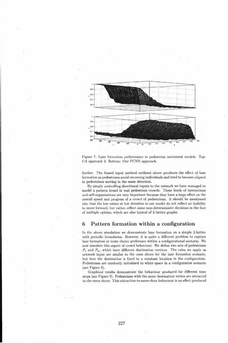
F'igure 7: Lane formation performance in pedestrian movement models. Top: CA approach 2. Bottom: Our PCNN approach.

fur ther. T he biased input method outlined above produces the effect of lane formation as pedestrians avoid oncoming individuals and tend to become aligned to pedestrians moving in the same direction.

By simply controlling directional inputs to the network we have managed to model a patLern fou nd in real pedestrian crowds. T hese kinds of interactions and self-organisations are very important because they have a large effect on the overall speed and progress of a crowd of pedestrians. It should be mentioned also tha t the low values at low densities in our model do not reflect an inability to move forward, but rather reflect some non-deterministic decisions in the face of mult iple optima, which are also typical of 2-lattice graphs.

6 Pattern formation within a configuration

In the above simulation we demonstrate lane formation on a simple 2-\atticc with periodic boundaries. However, it is quite a different problem to capture lane formation or route choice preference within a configurational scenario. We now simulate this aspect of crowd behaviour. We define two sets of pedestrians P. and Pw, which have different destination vertices. The rules we apply as network input are simila r to the ones above for the lane formation scenario, but here the destination is fixed to a constant location in the configuration. Pedestrians a re randomly initialised to white space in a configuration scenario (sec Figure 8}.

Graphical resul ts demonstrate the behaviour produced for different time steps (sec Figure 9}. Pedestrians with tl1e same destination vertex are attracted to the same doors. This attraction-to-san1e-door behaviour is an effect produced

227

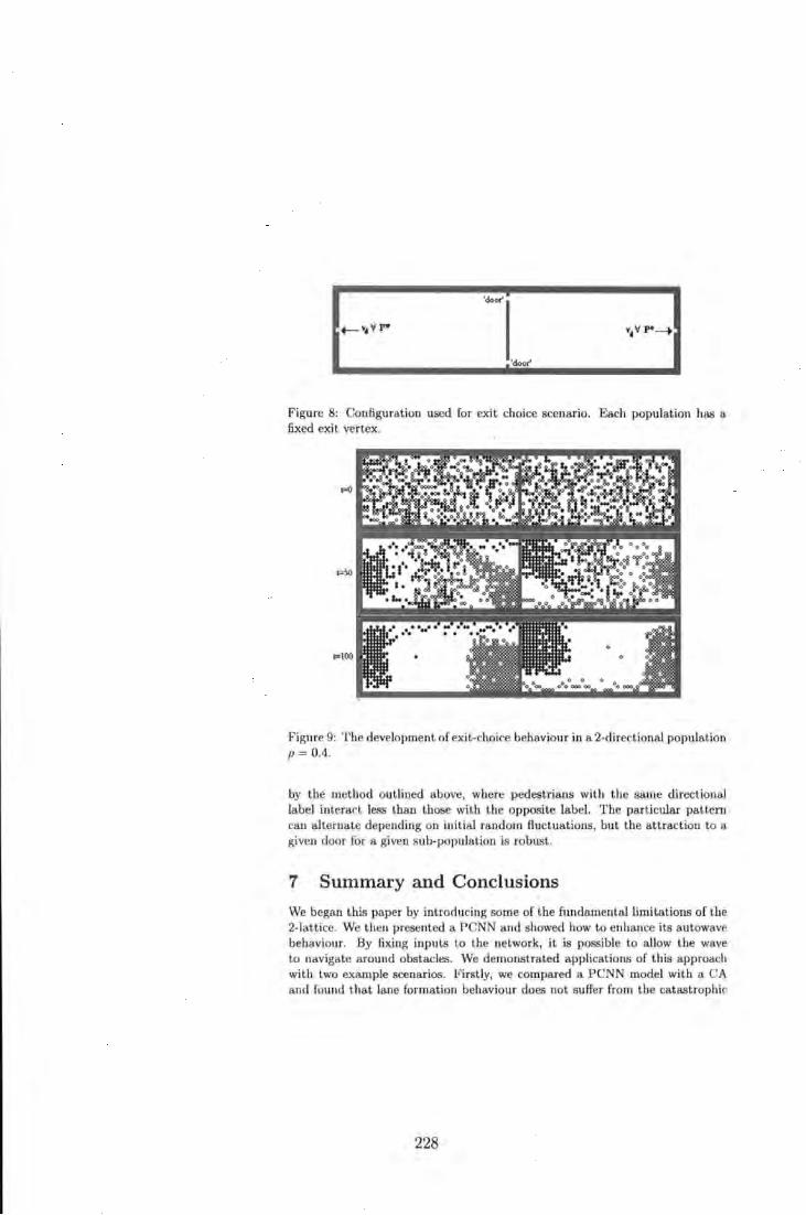
Figure 8: Configuration used for exit choice scenario. Each population has a fixed exit vertex.

Figure 9: The development of exit-choice behaviour in a 2-directional population p = 0.4.

by the method outlined above, where pedestrians with the same directional label interact less than those with the opposite label. The particular pattern can alternate depending on initial random fluctuations, but the attraction to a given door for a given sub-popula tion is robust.

7 Summary and Conclusions

We began this paper by introducing some of the fundamental limitations of the 2-lattice. We then presented a PCNN aud showed how to enhance its autowave behaviour. By fixing inputs to the network, it is possible to allow the wave to navigate around obstacles. We demonstrated applications of t his approach with two example scenarios. Firstly, we compared a PCNN model with a CA and found t ha t lane formation behaviour does not suffer from t he catastrophic

228

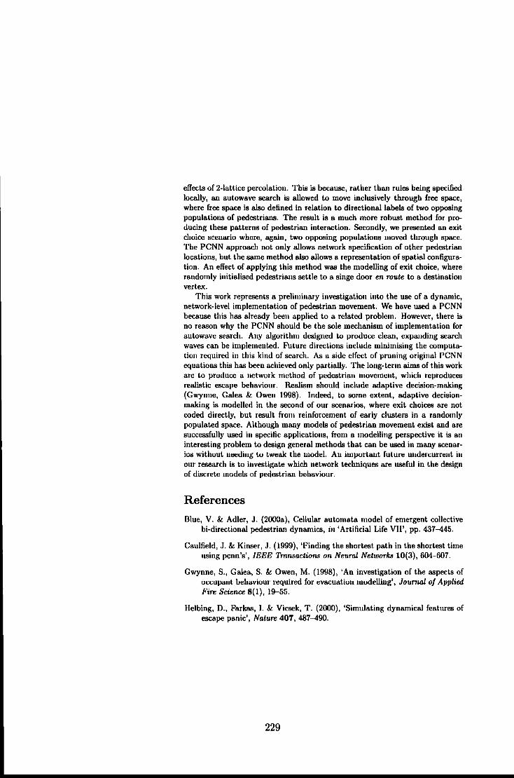
effects of 2-lattice percolation. This is becanse, rather than rules being specified locally, an autowave search is allowed to move inclusively through free space, where free space is also defined in relation to directional labels of two opposing populations of pedestrians. The result is a much more robust method for producing these patterns of pedestrian interaction. Secondly, we presented an exit choice scenario where, again, two opposing populations moved through space. The PCNN approach not only allows network specification of other pedestrian locations, but the same method also allows a representation of spatial configuration. An effect of applying this method was the modelling of exit choice, where randomly initialised pedestrians settle to a singe door en route to a destination vertex.

This work represents a preliminary investigation into the nse of a dynamic, network-level implementation of pedestrian movement. We have used a PCNN because this has already been applied to a related problem. However, there is no reason why the PCNN should be the sole mechanism of implementation for autowave search. Any algorithm designed to produce clean, expanding search waves can be implemented. FUture directions include minimising the computation required in this kind of search. As a side effect of pruning original PCNN equations this has been achieved only partially. The long-term aims of this work are to produce a network method of pedestrian movement, which reproduces realistic escape behaviour. Realism should include adaptive decision-making (Gwyuue, Galea &. Owen 1998). Indeed, to some extent, adaptive decisionmaking is modelled in the second of our scenarios, where exit choices are not coded directly, but result from reinforcement of early clusters in a randomly populated space. Although many models of pedestrian movement exist and are successfully used in specific applications, from a modelling perspective it is an interesting problem to design general methods that can be used in many scenarios without needing to tweak the model. An important future undercurrent in our research is to investigate which network techniques are nseful in the design of discrete models of pedestrian behaviour.

References

Blue, V. &. Adler, J. (2000a), Cellular automata model of emergent collective bi-directional pedestrian dynamics, in 'Artificial Life V11', pp. 437-445.

Caulfield, J. &. Kinser, J. (1999), 'Finding the shortest path in the shortest time using pcnn's', IEEE 1hmsactions on Neural Networks 10(3), 604-607.

Gwynne, S., Galea, S. &. Owen, M. (1998). 'An investigation of the aspects of occupant behaviour required for evacuation modelling', Joumal of Applied Fire Science 8(1), 19-55.

Helbing, D., Farkas, I. &. Vicsek, T. (2000), 'Simulating dynamical features of escape panic', Nature 407, 487-490.

229

Holden, R. & Cangelosi, A. (2004), Limits to locality in ceUular automata models of pedestrian behaviour, in 'lnterflam 2004, lOth International Fire Science and Engineering Conference', lnterscience, Edinburgh, pp. 761-766.

Lindblad, T. & Kinser, J. (1998), Image Proce8sing using Pulse-Coupled Neural Networks, Springer-Verlag, London.

Maass, W. & Bishop, C. (1998), Pulsed neuml networks, MIT Press, London.

Owen, M., Galea, E. & Lawrence, P. (1996), 'The exodus evacuation model applied to building evacuation scenarios', Joumal of Fire Protection Engineering 8(2). 65-86.

Schamschula, M., Johnson, J. & lnguva, R. (2000), Image processing with pulse coupled neural networks, in 'The Second International Forum on Multimedia and Image Processing', World Automation Congress, Maui, pp. 75--&l.

Sole, R. & Goodwin, B. (2000), Signs of Life: How complexity peroades biology, Basic Books, New York.

230

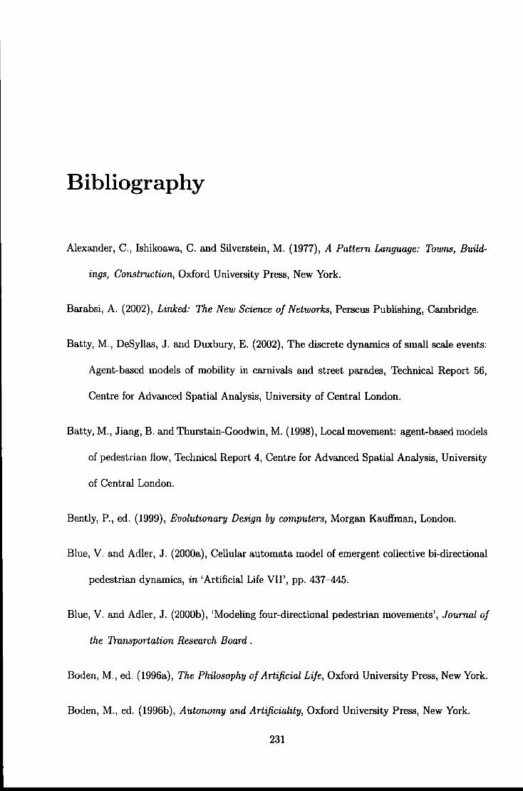
Bibliography

Alexander, C., Ishikoawa, C. and Silverstein, M. (1977), A Pattern Language: Towns, Build

ings, Construction, Oxford University Press, New York.

Barabsi, A. (2002), Linked: The New Science of Networks, Perseus Publishing, Cambridge.

Batty, M., DeSyllas, J. and Duxbury, E. (2002), The discrete dynamics of small scale events:

Agent-based models of mobility in carnivals and street parades, Technical Report 56,

Centre for Advanced Spatial Analysis, University of Central London.

Batty, M., Jiang, B. and Thurstain-Goodwin, M. (1998), Local movement: agent-based models

of pedestrian flow, Technical Report 4, Centre for Advanced Spatial Analysis, University

of Central London.

Bently, P., ed. (1999), Evolutionary Design by computers, Morgan Kauffman, London.

Blue, V. and Adler, J. (2000a), Cellular automata model of emergent collective bi-directional

pedestrian dynamics, in 'Artificial Life VII', pp. 437-445.

Blue, V. and Adler, J. (2000b), 'Modeling four-directional pedestrian movements', Journal of

the Transportation Research Board .

Boden, M., ed. (1996a), The Philosophy of Artificial Life, Oxford University Press, New York.

Boden, M., ed. (1996b), Autonomy and Artificiality, Oxford University Press, New York.

231

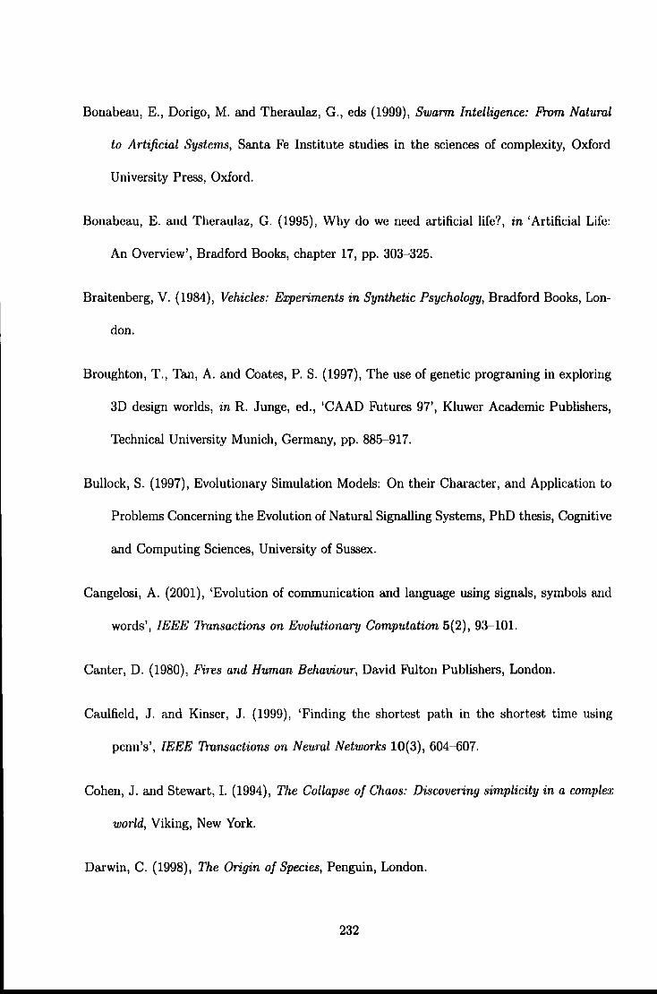
Bonabeau, E., Dorigo, M. and Theraulaz, G., eds (1999}, Swarm Intelligence: Prom Natuml

to Artificial Systems, Santa Fe Institute studies in the sciences of complexity, Oxford

University Press, Oxford.

Bonabeau, E. and Theraulaz, G. {1995}, Why do we need artificial life?, in 'Artificial Life:

An Overview', Bradford Books, chapter 17, pp. 303-325.

Braitenberg, V. {1984}, Vehicles: Experiments in Synthetic Psychology, Bradford Books, Lon

don.

Broughton, T., Tan, A. and Coates, P. S. (1997}, The use of genetic programing in exploring

3D design worlds, in R. Junge, ed., 'CAAD Futures 97', Kluwer Academic Publishers,

Technical University Munich, Germany, pp. 885-917.

Bullock, S. (1997}, Evolutionary Simulation Models: On their Character, and Application to

Problems Concerning the Evolution of Natural Signalling Systems, PhD thesis, Cognitive

and Computing Sciences, University of Sussex.

Cangelosi, A. (2001}, 'Evolution of communication and language using signals, symbols and

words', IEEE Transactions on Evolutionary Computation 5(2}, 93-101.

Canter, D. (1980}, Fires and Human Behaviour, David Fulton Publishers, London.

Caulfield, J. and Kinser, J. (1999}, 'Finding the shortest path in the shortest time using

pcnn's', IEEE Transactions on Neuml Networks 10(3}, 604--607.

Cohen, J. and Stewart, I. (1994}, The Collapse of Chaos: Discovering simplicity in a complex

world, Viking, New York.

Darwin, C. {1998}, The Origin of Species, Penguin, London.

232

Dawkins, R. (1976), The Selfish Gene, Oxford University Press, Oxford.

Dawkins, R. (1991), The Blind Watchmaker, Penguin, London.

Deneubourg, J., Goss, S., Franks, N., Sendova-Franks, A. and Detrain, C. (1990), 'The self

organising exploratory pattern of the argentine ant', Journal of Insect Behaviour 3, 159-

168.

Dennet, D. (1995), Darwin's Dangerous Idea: Evolution and the Meaning of Life, Penguin,

London.

D'Souza, R. and Margolus, N. (1999), 'A thermodynamically reversible generalisation of dif

fusion limited aggregation', Physical Review E 60(1).

Fahy, R. (2001), Verifying the predictive capability of exit89, in 'Human Behaviour and Fire',

MIT, Cambridge, Boston.

Feynman, R. (1963), The Feynman Lectures on Physics, Vol. 1, Addison-Wesley, London.

Feynman, R. (1992), The Character of Physical Law, Penguin, London.

Frazer, A. (1995), Evolutionary Architecture, Architectural Association, London.

Goldberg, D. (1989), Genetic Algorithms in Search, Optimisation and Machine Learning,

Addison-Wesley, Massachusetts.

Grand, S. (2000), Creation: Life and How To Make It, Weidenfeld and Nicolson, London.

Gwynne, S., Galea, S. and Owen, M. (1998), 'An investigation of the aspects of occupant

behaviour required for evacuation modelling', Journal of Applied Fire Science 8(1), 19-

55.

233

Halsey, T. (2000), 'Diffusion-limited aggregation: A model for pattern formation', Physics

Today 53(11).

Hamacher, H. and Tjandra, S. (2002), Mathematical modelling of evacuation problems: a

state of the art, in Schreckenberg and Sharma (2002), pp. 227-266.

Hanson, J. (1998), Decoding Homes and Houses, Cambridge University Press, Cambridge.

Harary, F., ed. (1997), Graph Theory and Statistical Physics, Academic Press, London.

Helbing, D., Farkas, 1., Molnr, P. and Vicsek, T. (2002), Simulation of pedestrian crowds in

normal and evacuation situations, in Schreckenberg and Sharma (2002), pp. 21-58.

Helbing, D., Farkas, I. and Vicsek, T. (2000), 'Simulating dynamical features of escape panic',

Nature 407, 487-490.

Helbing, D., Farkas, I. and Vicsek, T. (2001), 'Traffic and related self-driven many-particle

systems', Reviews of Modem Physics 73, 1067-1141.

Hillier, B. (1996), Space Is The Machine: A Configurational Theory of Architecture, Cam

bridge University Press, Cambridge.

Hillier, B. and Hanson, J. (1984), The Social Logic of Space, Cambridge University Press,

Cambridge.

Hillier, F. and Lieberrnan, G. (1990), Introduction to operations research, fifth edn, McGraw

Hill, London.

Holden, R. and Cangelosi, A. (2004a), A general computationally intelligent model for egress

simulation, in 'Interflam 2004, lOth International Fire Science and Engineering Confer

ence', lnterscience, Edinburgh, pp. 387-398.

234

Holden, R. and Cangelosi, A. {2004b), Limits to locality in cellular automata models of pedes

trian behaviour, in 'Interflam 2004, lOth International Fire Science and Engineering

Conference', Interscience, Edinburgh, pp. 761-766.

Holden, R. and Parmee, I. {2000), Evolutionary spatial layout utilising agent-based models

of crowd behaviours, in 'Poster Proceedings of the Fourth International Conference on

Evolutionar Design and Manufacture', University of Plymouth, Plymouth.

Holden, R., Sanjana, N. and Seiferle-Valencia, A. {2002), The diffusion of ideas on dynamic

social networks, in 'Student Paper Proceedings of Complex Systems Summer School',

The Santa Fe Institute, Santa Fe.

Holland, J. {1975), Adaptation in Natuml and Artificial Systems, The University of Michigan

Press., Ann Arbour.

Holland, J. {1995), How Adaptation Builds Complexity, Bradford Books, Bradford.

Holldobler, B. and Wilson, E. 0. {1990), The Ants, Harvard University Press.

Huggert, N. {1999), Space from Zeno to Einstein, Bradford Books, London.

Hughes, R. {2002), 'A continuum theory of pedestrian motion', Tronsporlation Research B

pp. 50Q-535.

Hughes, R. {2003), 'The flow of human crowds', Annual Review of Fluid Mechanics pp. 169-

182.

Jennings, N. {1998), 'Editorial', Autonomous agents and multi-agent systems 1{1), 1-2.

Jin, E., Girvan, M. and Newman, M. {2001), The structure of growing social networks, Tech

nical Report 32, Santa Fe Institute, Santa Fe, New Mexico.

235

Johnson, J. {1994), The signature of images, in 'IEEE International Conference on Neural

Networks', Orlando.

Jones, J. K. M. B. K. L. J. {1996), Modelling vehicle behaviour in congested networks using

highly parallel systems, in 'Proceedings of the 24th European Transport Forum'.

Kauffman, S. {1995), At Home in the Universe: The Search for Laws of Complexity, Oxford

University Press, New York.

Kerridge, R. K J. (2001), Pedflow: Development of an autonomous agent model of pedestrian

flow, in '80th Annual Meeting TRB - Spatial Analysis in Urban Activity and Travel

Demand Modelling', Washington DC.

Kimura, M. {1983), The Neutml Theory of Molecular Evolution, Cambridge University Press.

Kumar, S. and Bentley, P., eds {2003), On Growth, Form and Computers., Elsevier Academic

Press, London.

Langton {1996a), Artificial life, in Boden {1996a), chapter??, p. ??

Langton, C. {1990), 'Computation at the edge of chaos: phase transitions and emergent

computation', Physica D 42, 12-37.

Levy, S., ed. {1993), Artificial Life: The Quest for a New Creation, Penguin, London.

Lindblad, T. and Kinser, J. {1998), Image Processing using Pulse-Coupled Neuml Networks,

Springer-Verlag, London.

Maass, W. and Bishop, C. {1998), Pulsed neuml networks, MIT Press, London.

Maynard-Smith, J. {1974), Models in Ecology, Cambridge University Press, Cambridge.

236

Michalewicz, Z. {1999), Genetic algorithms + Data Structures = Evolution Programs, third

edn, Springer, London.

Miller, G. (1995), Artificial life as theoretical biology: How to do real science with com

puter simulation, Technical Report 378, Cognitive and Computing Science, University of

Sussex.

Mitchell, M. {1999), An Introduction to Genetic Algorithms, Bradford Books, London.

Mitchell, M. and Crutchfield, J. (1996), Evolving cellular automata with genetic algorithms:

A review of recent work, in 'Proceedings of the First International Conference on Evolu

tionary Computation and Its Applications'.

Muhlenbein, H. and Shlierkamp-Voosen, D. ( 1993), 'Predictive models for the breeder genetic

algorithm: I. continuous parameter optimization', Evolutionary Computation 1(1), 25-

49.

Nagel, K. and Rasmussen, S. {1994), Traffic at the edge of chaos, in 'Artificial Life IV: Pro

ceedings of the Fourth International Workshop on the Synthesis and Simulation of Living

Systems'.

Newman, M. {2003), 'Properties of highly clustered networks', Physical Review E 68.

Noble, J. (1998), The Evolution of Animal Communication Systems: Questions of function

examined through simulation, PhD thesis, Cognitive and Computing Science, University

of Sussex.

O'Reilly, U. M. and Testa, P. (2000), Representation in architectural design tools, in Parmee

{2000).

237

Owen, M., Galea, E. and Lawrence, P. (1996), 'The exodus evacuation model applied to

building evacuation scenarios', Journal of Fire Protection Engineering 8(2), 65-86.

Owen, M., Galea, E., Lawrence, P. and Filippidis, L. (1998), 'The numerical simulation of air

craft evacuation and its application to aircraft desigu and certification', The Aeronautical

Journal pp. 301-312.

Parmee, 1., ed. (2000), ACDM: Proceedings of the Conference on Adaptive Computing in

Design and Manufacture, University of Plymouth, Kluwer academic publishers, London.

Penn, A. and Thrner, A. (2002), Space syntax based agent simulation, in Schreckenberg and

Sharma (2002), pp. 99-114.

Peponis, J., Zimring, C. and Choi, Y. (1990), 'Finding the building in wayfinding', Environ

ment and Behaviour 22(5), 555-590.

Prusinkiewicz, P. (1995), Visual models of morphogenesis, in 'Artificial Life: An Overview',

Bradford Books, pp. 61-74.

Raubal, M. (2001), Agent-based Simulation of Human Wayfinding: A Perceptual Model for

Unfamiliar Buildings, PhD thesis, Vienna University of Technology, Vienna.

Resnick, M. (1994), Turtles, Ten11itcs and Traffic Jams: Explomtions in Massively Pamllel

Microworlds, MIT Press, Cambridge.

Reynolds, C. (1987), 'Flocks, herds, and schools: A distributed behavioral model', Computer

Gmphics 21(4), 25-34.

Reynolds, C. (1999), Steering behaviours for autonomous characters, in 'Proceedings of the

Game Developers Conference', pp. 763-782.

238

Rosenman, M. (1996), The generation of form using an evolutionary approach, in J. Gero,

eel., 'Artificial Intelligence '96', Kluwer Academic Press, London, pp. 643--662.

Schamschula, M., Johnson, J. and Inguva, R. (2000), Image processing with pulse coupled neu

ral networks, in 'The Second International Forum on Multimedia and Image Processing',

World Automation Congress, Maui, pp. 75-86.

Schreckenberg, M. and Sharma, S., eds (2002), Pedestrian and Evacuation Dynamics. Proceed

ings of the First Conference on Pedestrian and Evacuation Dynamics, Springer, Berlin.

Schuster, P. (1997), Extended Molecular Evolutionary Biology, Bradford Books, London, chap

ter 3, pp. 39--60.

Shipman, R. (2003), Coupling Evolution and Self-Organisation in Bio-lnspired Communica

tion Systems, PhD thesis, School of Computing, University College London.

Sole, R. and Goodwin, B. (2000), Signs of Life: How complexity pervades biology, Basic Books,

New York.

Stanley, A. (1992), Walk this way: using agent-based simulation to evaluate architectural

designs, Master's thesis, COGS, University of Sussex.

Stanley, K. and Miikkulainen, R. (2003), 'Taxonomy for artificial embryogeny', Artificial Life

9(2), 93-130.

Staulfer, D. and Aharony, A. (1992), Introduction to Percolation Theory, Taylor Francis,

London.

Stewart, I. (1997), Does God Play Dice: The new maths of chaos, Penguin, London.

Still, K. (2000), Crowd Dynamics, PhD thesis, Mathematics, University of Warwick.

239

Suzudo, T. (2002), Diversity of complex systems produced by a class of cellular automata, in

'Proceedings of the 6th International Conference on Complex Systems', Tokyo.

Torrens, P. (2000), How cellular models of urban systems work (1 theory), Technical Report 28,

Centre for Advanced Spatial Analysis, University of Central London.

Watts, D. (1999), Small Worlds: The Dynamics of Networks Between Order and Randomness,

Princeton Studies in the Science of Complexity, Princeton.

Wheeler, M. (1996), From robots to rothko: The bringing forth of worlds, in M. Boden, ed.,

'The Philosophy of Artificial Life', Oxford University Press.

Wilson, R. (1985), Introduction to Gmph Theory, third edn, Longman, New York.

Wilson, W. (2000), Simulating Evolutionary and Ecological Systems in C, Cambridge Univer

sity Press, Cambridge.

Witten, T. and Sadler, L. (1983), 'Diffusion-limited aggregation', Physical Review B 27, 5686-

5697.

Wolfram, S. (1984), 'Universality and complexity in cellular automata', Physica D 10, 1-35.

Wolfram, S. (2002), A New Kind of Science, Wolfram Media Inc, Illinois.

Wright, S. (1932), The roles of mutation inbreeding, crossbreeding and selection in evolution,

in 'International proceedings of the congress on genetics', pp. 356-366.

240

DOCTOR OF PHILOSOPHY - CORE

Documents