UNIVERSITÉ PIERRE & MARIE CURIE - SORBONNE UNIVERSITÉS Doctor of Philosophy (Ph.D.) Thesis to obtain the title of PhD of Science of the University Pierre & Marie Curie Specialty : Applied Mathematics Defended by Quang Dien Duong Application of advanced statistical analysis for internal modeling in life insurance Thesis Advisor: Agathe Guilloux and Olivier Lopez defended on Mars 4, 2021 Jury : Reviewers : Mathieu Ribatet - École Centrale de Nantes Frédéric Planchet - Université Claude Bernard - Lyon 1 Advisors : Agathe Guilloux - Université d’Évry Val d’Essonne Olivier Lopez - Université Pierre & Marie Curie Examinators : Michel Broniatowski - Sorbonne Université Caroline Hillairet - ENSAE Thomas Lim - ENSIIE Evry

Welcome message from author
This document is posted to help you gain knowledge. Please leave a comment to let me know what you think about it! Share it to your friends and learn new things together.
Transcript

UNIVERSITÉ PIERRE & MARIE CURIE - SORBONNEUNIVERSITÉS
Doctor of Philosophy (Ph.D.)Thesis
to obtain the title of
PhD of Science
of the University Pierre & Marie CurieSpecialty : Applied Mathematics
Defended by
Quang Dien Duong
Application of advanced statisticalanalysis for internal modeling in
life insurance
Thesis Advisor: Agathe Guilloux and Olivier Lopez
defended on Mars 4, 2021
Jury :
Reviewers : Mathieu Ribatet - École Centrale de NantesFrédéric Planchet - Université Claude Bernard - Lyon 1
Advisors : Agathe Guilloux - Université d’Évry Val d’EssonneOlivier Lopez - Université Pierre & Marie Curie
Examinators : Michel Broniatowski - Sorbonne UniversitéCaroline Hillairet - ENSAEThomas Lim - ENSIIE Evry


Acknowledgments
First of all, I would like to thank Prof. Mathieu Ribatet and Prof. Frédéric Planchetfor agreeing to review this thesis. The final version of this thesis benefited from theirvery careful reading and their valuable comments. I also thank all the members ofthe jury for agreeing to attend the presentation of this work.
Second, I owe my deepest gratitude to my PhD supervisors, Prof. Agathe Guil-loux and Prof. Olivier Lopez. Agathe and Olivier, I would like to thank you forthe kindness you have shown toward my work and myself over the past four years.Thank you for sharing with me your scientific knowledge and rigor; they both per-meate throughout my PhD thesis today.
I would also like to thank Jean-Baptiste Monnier for being such a great PhDadviser and scientific interlocutor. Jean-Baptiste, thank you for your enlighteningscientific advices, for being so welcoming and for your great sense of humor. Moreimportantly, I would like to thank you for your constant encouragements, especiallywhen times were tougher, and for the enjoyable times spent in your office or arounda cup of coffee; I hope there will be many more.
My thanks also go to the members of the Risk and Value Measurement Servicesteam and especially Vincent Gibrais, Emmanuel Perrin, Bastien Godrix, DidierRiche and Santiago Hector Fiallos. These meetings were very enriching and we wereable to work together and share discussions on many exciting topics.


Contents
1 Introduction 11.1 Presentation of the PwC’s R&D project . . . . . . . . . . . . . . . . 11.2 Context of the study . . . . . . . . . . . . . . . . . . . . . . . . . . . 21.3 Problems with calculating the distribution of basic own funds over a
one-year time horizon . . . . . . . . . . . . . . . . . . . . . . . . . . 41.4 Proxy models in life insurance . . . . . . . . . . . . . . . . . . . . . . 7
1.4.1 Curve-Fitting . . . . . . . . . . . . . . . . . . . . . . . . . . . 81.4.2 Least Square Monte-Carlo . . . . . . . . . . . . . . . . . . . . 81.4.3 Replicating Portfolios . . . . . . . . . . . . . . . . . . . . . . 121.4.4 Acceleration algorithm . . . . . . . . . . . . . . . . . . . . . . 14
1.5 Error quantification for internal modeling in life insurance . . . . . . 151.6 Application of Extreme Value Theory to Solvency Capital Require-
ment estimation . . . . . . . . . . . . . . . . . . . . . . . . . . . . . . 161.7 Contributions and structure of the thesis . . . . . . . . . . . . . . . . 17
1.7.1 Contribution to the company . . . . . . . . . . . . . . . . . . 171.7.2 Methodological contributions . . . . . . . . . . . . . . . . . . 181.7.3 Structure of the thesis . . . . . . . . . . . . . . . . . . . . . . 27
2 Solvency II - Interpreting the key principles of Pillar I 292.1 History of capital requirements in the European insurance industry . 29
2.1.1 Solvency I directive . . . . . . . . . . . . . . . . . . . . . . . . 292.1.2 From Solvency I to Solvency II . . . . . . . . . . . . . . . . . 30
2.2 Implementation of Solvency II . . . . . . . . . . . . . . . . . . . . . . 312.3 Pillar I . . . . . . . . . . . . . . . . . . . . . . . . . . . . . . . . . . . 32
2.3.1 The quantitative requirements of Pillar 1 . . . . . . . . . . . 332.3.2 Standard Formula . . . . . . . . . . . . . . . . . . . . . . . . 352.3.3 Internal Model . . . . . . . . . . . . . . . . . . . . . . . . . . 38
3 Application of Bayesian penalized spline regression for internalmodeling in life insurance 393.1 Univariate nonparametric regression . . . . . . . . . . . . . . . . . . 40
3.1.1 Kernel smoothing method . . . . . . . . . . . . . . . . . . . . 413.1.2 Spline regression . . . . . . . . . . . . . . . . . . . . . . . . . 43
3.2 Multivariate non-parametric regression . . . . . . . . . . . . . . . . . 453.2.1 Some problems in high dimensional analysis . . . . . . . . . . 463.2.2 Dimension Reduction Techniques . . . . . . . . . . . . . . . . 463.2.3 Additive models . . . . . . . . . . . . . . . . . . . . . . . . . 47
3.3 Notations and requirements for the fitting process . . . . . . . . . . . 493.3.1 Risk factors . . . . . . . . . . . . . . . . . . . . . . . . . . . . 493.3.2 Loss function . . . . . . . . . . . . . . . . . . . . . . . . . . . 50

iv Contents
3.3.3 Approximation of a shock at t = 0+ . . . . . . . . . . . . . . 513.4 Methodology description . . . . . . . . . . . . . . . . . . . . . . . . . 523.5 Numerical study . . . . . . . . . . . . . . . . . . . . . . . . . . . . . 57
3.5.1 ALM modeling . . . . . . . . . . . . . . . . . . . . . . . . . . 573.5.2 Analysis of the loss functions . . . . . . . . . . . . . . . . . . 603.5.3 Nested Simulations . . . . . . . . . . . . . . . . . . . . . . . . 69
4 Sparse group lasso additive modeling for Pareto-type distributions 714.1 Part I - Overview of Extreme Values Theory . . . . . . . . . . . . . . 72
4.1.1 Generalized extreme value distribution . . . . . . . . . . . . . 724.1.2 Peak-over-threshold method . . . . . . . . . . . . . . . . . . . 744.1.3 Example of limiting distributions . . . . . . . . . . . . . . . . 754.1.4 Statistical Estimation . . . . . . . . . . . . . . . . . . . . . . 774.1.5 Characterisation of Maximum Domains of Attraction . . . . . 79
4.2 Part II - Sparse group lasso additive modeling for conditional Pareto-type distributions . . . . . . . . . . . . . . . . . . . . . . . . . . . . . 794.2.1 Methodology . . . . . . . . . . . . . . . . . . . . . . . . . . . 804.2.2 Simulation Study . . . . . . . . . . . . . . . . . . . . . . . . . 89
4.3 Appendix . . . . . . . . . . . . . . . . . . . . . . . . . . . . . . . . . 984.3.1 Proof of Lemma 1 . . . . . . . . . . . . . . . . . . . . . . . . 984.3.2 Best approximation by splines . . . . . . . . . . . . . . . . . . 984.3.3 Block Coordinate Descent Algorithm . . . . . . . . . . . . . . 99
5 Conclusion 101
A Economic Scenarios Modeling 105A.1 Correlated random vectors generator . . . . . . . . . . . . . . . . . . 106A.2 Hull White Model . . . . . . . . . . . . . . . . . . . . . . . . . . . . 108
A.2.1 Cap pricing . . . . . . . . . . . . . . . . . . . . . . . . . . . . 110A.3 Black Scholes Model . . . . . . . . . . . . . . . . . . . . . . . . . . . 112A.4 Jarrow, Lando and Turnbull Model . . . . . . . . . . . . . . . . . . . 117
A.4.1 Transition process . . . . . . . . . . . . . . . . . . . . . . . . 119A.4.2 Spread . . . . . . . . . . . . . . . . . . . . . . . . . . . . . . . 121A.4.3 Model Calibration . . . . . . . . . . . . . . . . . . . . . . . . 121
B Asset-Liability Management 125B.1 Introduction . . . . . . . . . . . . . . . . . . . . . . . . . . . . . . . . 125B.2 Saving contract . . . . . . . . . . . . . . . . . . . . . . . . . . . . . . 126
B.2.1 Characteristics of a saving contract . . . . . . . . . . . . . . . 127B.2.2 Accounting in insurance companies-Basic concepts . . . . . . 129
B.3 General presentation of the ALM simulator . . . . . . . . . . . . . . 130B.3.1 Description of the Asset . . . . . . . . . . . . . . . . . . . . . 131B.3.2 Description of the Liability . . . . . . . . . . . . . . . . . . . 135B.3.3 Chronology of the Asset-Liability interactions . . . . . . . . . 139

Contents v
B.3.4 Profit-sharing strategy . . . . . . . . . . . . . . . . . . . . . . 140B.3.5 End-of-period liabilities modeling . . . . . . . . . . . . . . . . 146
B.4 ALM modeling consistency - Leakage test . . . . . . . . . . . . . . . 146
C Demonstration of the θt equation 151
D Bayesian P-spline regression and Bayesian asymptotic confidenceinterval 153D.1 Smoothing Splines . . . . . . . . . . . . . . . . . . . . . . . . . . . . 153D.2 Regression Penalized Splines or P-Splines . . . . . . . . . . . . . . . 154D.3 Bayesian Analysis for Penalized Splines Regression . . . . . . . . . . 155D.4 Bayesian Asymptotic Confidence Interval . . . . . . . . . . . . . . . . 155D.5 Additive model and Asymptotic confidence interval for each func-
tional components . . . . . . . . . . . . . . . . . . . . . . . . . . . . 157D.6 Upper bound of the probabilities of deviation . . . . . . . . . . . . . 158D.7 Best approximation by splines . . . . . . . . . . . . . . . . . . . . . . 159D.8 Asymptotic distribution of empirical quantiles . . . . . . . . . . . . . 160
Bibliography 161


Chapter 1
Introduction
Contents1.1 Presentation of the PwC’s R&D project . . . . . . . . . . . . 11.2 Context of the study . . . . . . . . . . . . . . . . . . . . . . . 21.3 Problems with calculating the distribution of basic own
funds over a one-year time horizon . . . . . . . . . . . . . . . 41.4 Proxy models in life insurance . . . . . . . . . . . . . . . . . . 7
1.4.1 Curve-Fitting . . . . . . . . . . . . . . . . . . . . . . . . . . . 81.4.2 Least Square Monte-Carlo . . . . . . . . . . . . . . . . . . . . 81.4.3 Replicating Portfolios . . . . . . . . . . . . . . . . . . . . . . 121.4.4 Acceleration algorithm . . . . . . . . . . . . . . . . . . . . . . 14
1.5 Error quantification for internal modeling in life insurance 151.6 Application of Extreme Value Theory to Solvency Capital
Requirement estimation . . . . . . . . . . . . . . . . . . . . . 161.7 Contributions and structure of the thesis . . . . . . . . . . . 17
1.7.1 Contribution to the company . . . . . . . . . . . . . . . . . . 171.7.2 Methodological contributions . . . . . . . . . . . . . . . . . . 181.7.3 Structure of the thesis . . . . . . . . . . . . . . . . . . . . . . 27
1.1 Presentation of the PwC’s R&D project
Research and Development ("R&D") is a very important focus for the developmentof PricewaterhouseCoopers Advisory. Indeed, the consulting activity requires aconstant level of excellence and needs to be constantly at the forefront of innovation.For this reason, PricewaterhouseCoopers Advisory invests in a strong R&D policyand conducts dozens of internal and clients R&D projects every year.
PricewaterhouseCoopers Advisory conducts research in various scientific andtechnological fields. Thus, several R&D projects are conducted in major scien-tific disciplines such as mathematics and financial statistics, Big Data, computersecurity, etc.
In addition, PricewaterhouseCoopers Advisory has set up a department called"Risk and Value Measurement Services" (or "RVMS"). It is a unique center ofexpertise working with the "financial industry" (major players in the insurance andbanking sectors) to respond to their challenges in terms of risk and value.

2 Chapter 1. Introduction
The "RVMS" cluster brings together nearly 70 modeling and risk experts (ac-tuaries, quantitative engineers and data scientists). These experts master both thequantitative techniques and the functional, operational and regulatory environmentin which these techniques are used (Solvency II, Basel III, IFRS evolution, etc.).Trained in auditing methods, they also have significant experience in conductingcomplex consulting missions.
This team, which relies on in-house technical studies, is organized to meet theexpectations of PricewaterhouseCoopers Advisory clients. It also uses Pricewater-houseCoopers’ international network to be at the forefront of actuarial methods,tools and quantitative finance.
The RVMS department supervise a CIFRE thesis in partnership with the Pierreand Marie Curie University (Paris 6). This CIFRE thesis entitled "Application ofadvanced statistical analysis for internal modeling in life insurance" aims to developinnovative methods to effectively address the complex problem posed by the valu-ation of life insurance commitments and the calculation of their prudential capitalcost, and is an integral part of the research project that will be described later inthis document.
1.2 Context of the study
The valuation of life insurance liabilities presents real complexity, since it is based inparticular on profit-sharing mechanisms which require the simultaneous modeling ofthese liabilities with the asset items associated with them. This complexity is natu-rally multiplied in the context of prudential capital calculations by internal models,given that it is then a question of obtaining the distribution of these valuations atone year, in accordance with article 121 of the Solvency 2 directive (please refer toProblem 1 in Section 1.3 for more details). To reduce the degree of complexity ofthis problem, various approximation, better known under the name of proxy modelsor loss functions, are proposed in practice. We will detail later how these proxymodels are validated in practice and the efforts that remain to be made to improvetheir reliability. In particular, we suggest justifying the choice of the method usedduring the validation step of the loss functions. But first, how are life insuranceliabilities valued in practice?
In practice, life insurance liabilities are valued using the risk-neutral Monte-Carlomethod. This method consists of estimating the value of life insurance commitmentsas the average of the discounted values at the risk-free rate of benefits paid topolicyholders for a set of financial trajectories called risk neutral scenarios. Thisvaluation method captures the optionality of life insurance liabilities and gives theman economic value, also known as "market consistent". You might ask "Wheredoes the optionality of life insurance liabilities come from?"
Conventional life insurance contracts with a savings component usually offertheir holders a number of guarantees. Among the main guarantees are minimumguaranteed rates, profit sharing and the right of redemption. Depending on the

1.2. Context of the study 3
contracts, we can also find the cancellation option in annuity, the right to arbitratebetween support in EURO and support in Unit-Linked (UL), the UL floor guaranteein the event of death, etc. These guarantees represent rights granted by life insurersto their policyholders and can be considered as options in all respects similar tothose treated on the financial markets.
What is the typical calculation time for the economic value of a lifeinsurance liability? Depending on the size of the balance sheet, the complexityof the optionality of life insurance contracts and the finesse of the cash-flow modelused, the “market-consistent” valuation of a life insurer’s commitments can rangefrom several minutes to several hours. The same is therefore true for the valuationof its own funds.
The Solvency II directive offers life insurers the possibility of using a (partial)internal model in order to assess the forecast probability density of the variationin their own funds over one year (see article 121) and in particular its quantile at99.5% called “Solvency Capital Requirement” (SCR). In practice, this quantile isestimated by the Monte-Carlo method. This method consists of simulating severaltens of thousands of future economic and actuarial environments within one year,revaluing the equity (and therefore the liabilities) of the life insurance company ineach of these new states of the world, and identify the annual change in equityassociated with the 99.5% percentile.
Given the time required to calculate the value of a life insurance company’sown funds using a cash-flow model in a given economic and actuarial environment,the abrupt calculation of the SCR by the Monte- Carlo is not possible in practice.In order to solve this problem, life insurance undertakings have developed "proxy"methods intended to reproduce the results of the cash flow model in a very shorttime and in any economic and actuarial environment.
So what are the proxy methods that are used in practice? The economicand actuarial environment of a life insurance company is in practice modeled by avector of risk factors. The cash-flow model is therefore a function in the mathemat-ical sense of the term which associates a specific background value with a vector ofrisk factors. This function will be referred to below as the “equity function”. Proxymodels are therefore ultimately approximations or estimators of the value of equityfunction. The problem of approximating the value of equity function is a complexproblem. Its complexity is in practice all the greater as the dimension of the un-derlying risk factor vector is large and the regularity of the equity function is low.Given the inherent difficulty of this problem, no technical solution has yet emergedas being the most appropriate, and a multitude of approaches coexist, each with itsown advantages and disadvantages. The best known and also the most frequentlyused are the Curve-Fitting, Least Square Monte Carlo (LSMC) and ReplicatingPortfolio methods (see Section 1.4 for more details).
How are these proxy models validated in practice? Is there a regulatoryrequirement for error controlling. As stated in Article 229-(g) of the DelegatedActs [93], deviations caused by the use of these proxy models must be measuredand controlled. The validation of these proxy models therefore essentially consists

4 Chapter 1. Introduction
in developing robust procedures for measuring and controlling the error introducedby the use of the proxy model.
In the first part of this thesis, we will introduce a novel proxy method, whichis highly practical, modular, smooth and naturally relates the approximation errorsto the Monte-Carlo statistical errors. Furthermore, our approach allows insurancecompanies to naturally and transparently start reporting confidence levels on theirprudential reporting, which is not disclosed so far by insurance companies and wouldbe a relevant information within solvency disclosures for the industry.
In the second part of this thesis, we will deal with the quantile estimation prob-lem when the tail distribution is heavy and covariate information is available. Tothis end, we rely on extreme value statistics.
In extreme value statistics, estimation of the tail-index is of importance in nu-merous applications since it measures the tail heaviness of a distribution. Examplesinclude heavy rainfalls, big financial losses, high medical costs, just to name a few.When covariate information is available, we are mainly interested in describing thetail heaviness of the conditional distribution of the dependent variable given theexplanatory variables and the tail-index will be thus taken as a function of this co-variate information. In many practical applications, the explanatory variables cancontain hundreds of dimensions. Many recent algorithms use concepts of proximityin order to estimate model parameters based on their relation to the rest of thedata. However, in high dimensional space, the data is often sparse and the notionof proximity fails to retain its meaningfulness. Therefore, this implies deteriorationin estimation. The main purpose of this study is thus to overcome this challenge inthe context of the tail-index estimation given the explanatory variables.
1.3 Problems with calculating the distribution of basicown funds over a one-year time horizon
Recall that the Solvency Capital Requirement (SCR) is defined as the economic cap-ital to be held to ensure that ruin occurs over a one-year horizon with a probabilityunder 0.5%. Mathematically, the SCR is defined as follows:
P (BOFt=1 < 0 | BOFt=0 ≥ SCR) ≤ 0.5%
where P is the historical probability measure and BOF stands for the Basic OwnFunds defined as the difference between the Asset value within the economical bal-ance sheet and the Best Estimate liabilities (BEL). Note that the determination ofthe Basic Own Funds does not include the risk margin to avoid the problem of circu-larity that the introduction of this notion induces. Given the implicit nature of thedefinition given above, Bauer et al. [8] introduced a approximately equivalent notionof the SCR. In their paper, they define the SCR as the 99.5%-quantile of the oneyear loss function, evaluated at t = 0, which is of the form BOFt=0−P (0, 1)BOFt=1
with P (0, 1) the discount factor. Namely, we have
SCR = arg minu
P (BOFt=0 − P (0, 1)BOFt=1 > u) ≤ 0.5%
1.3. Problems with calculating the distribution of basic own funds overa one-year time horizon 5
or equivalentlySCR = BOFt=0 − P (0, 1)q0.5% (BOFt=1) . (1.1)
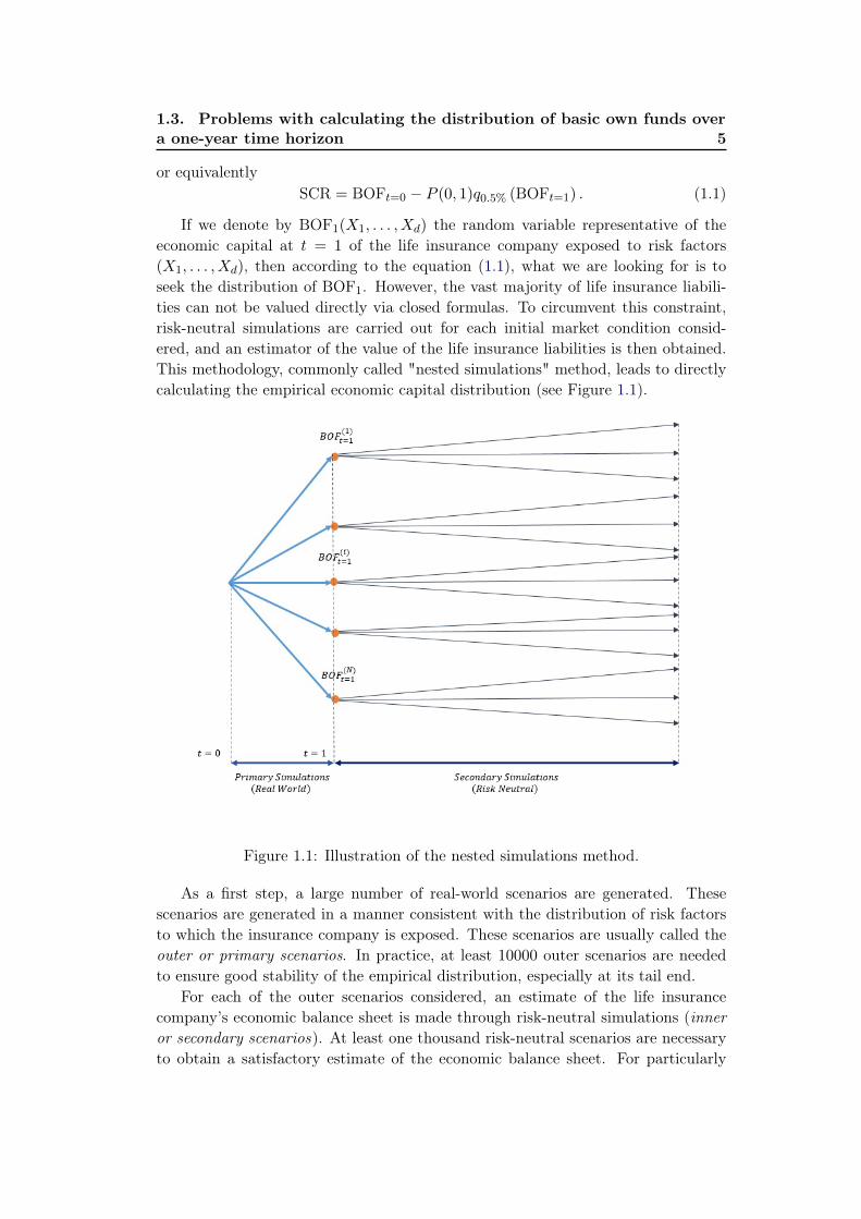
If we denote by BOF1(X1, . . . , Xd) the random variable representative of theeconomic capital at t = 1 of the life insurance company exposed to risk factors(X1, . . . , Xd), then according to the equation (1.1), what we are looking for is toseek the distribution of BOF1. However, the vast majority of life insurance liabili-ties can not be valued directly via closed formulas. To circumvent this constraint,risk-neutral simulations are carried out for each initial market condition consid-ered, and an estimator of the value of the life insurance liabilities is then obtained.This methodology, commonly called "nested simulations" method, leads to directlycalculating the empirical economic capital distribution (see Figure 1.1).
Figure 1.1: Illustration of the nested simulations method.
As a first step, a large number of real-world scenarios are generated. Thesescenarios are generated in a manner consistent with the distribution of risk factorsto which the insurance company is exposed. These scenarios are usually called theouter or primary scenarios. In practice, at least 10000 outer scenarios are neededto ensure good stability of the empirical distribution, especially at its tail end.
For each of the outer scenarios considered, an estimate of the life insurancecompany’s economic balance sheet is made through risk-neutral simulations (inneror secondary scenarios). At least one thousand risk-neutral scenarios are necessaryto obtain a satisfactory estimate of the economic balance sheet. For particularly

6 Chapter 1. Introduction
extreme outer scenarios, the number of risk-neutral simulations to be carried outcan be even greater.
In theory, this methodology is the one that achieves the most accurate economicown funds distribution. However, its implementation on a large scale still seemsimpossible today. Here we try to decompose very briefly the cycle of calculation ofthe economic own funds distribution.
• Outer scenarios generation: This step is by itself not particularly complex, aswe seek in the solvency 2 regulatory framework to measure the variation ineconomic own funds for extreme quantiles, it is important to have sufficientouter scenarios to ensure good stability of the empirical SCR estimate.
• Building economic balance sheets: As previously explained, it is necessary toperform risk-neutral valuations for each outer scenarios. These valuation pro-cesses require the dissemination of risk-neutral scenarios based on the achieve-ment of real-world risk factors. Depending on the complexity of the modelsused, this step may require many hours of calculation.
Today, the majority of ALM models used by insurance companies would be too slowto calculate the economic own funds distribution using this methodology. Put, end-to-end, this process does not seem possible nowadays. The constant improvementof diffusion models, projection models and the progress of information technologyshould enable us to improve these computing times in the future. But today weare still too far from the target to implement this methodology within life insurancecompanies.
In fact, we have only considered the production time so far, we must not neglectthe time required to analyze these results. As it stands, life insurers encounter aproduction time problem which can be formulated as follows :
Problem 1: The calculation of the Basic own Funds in life insurance is madeparticularly complex by many interactions between and liabilities, and is required alarge number of simulations to obtain a satisfactory result as a consequence of the lawof large numbers. The asset-liabilities interactions are related to the profit sharingmechanisms which are derived from both business objectives (client retention) andaccounting rules. Profit sharing impacts then the liabilities through the changes infuture services and the impacts it may have on policyholder behavior. The timenecessary to compute a BOF corresponding to with-profit saving contracts can varybetween about 10 min and 1 h depending on the computing power available and thecomplexity of the underlying cash-flows models. Assume that an insurer uses from104 to 2 × 10⁵ real world scenarios to derive the SCR and that the BOF is to becomputed in 10 min, this would amount to minimum 105 min, that is 70 days or 10
weeks of computation time. As a result, the nested simulation or brute-force approachis unsuitable since it leads to significant computing times, while these processes mustbe implemented in a very short amount of time for reporting purposes. Accordingto the Technical Practices Survey conducted by KPMG in 2015 [70], the majority of
1.4. Proxy models in life insurance 7
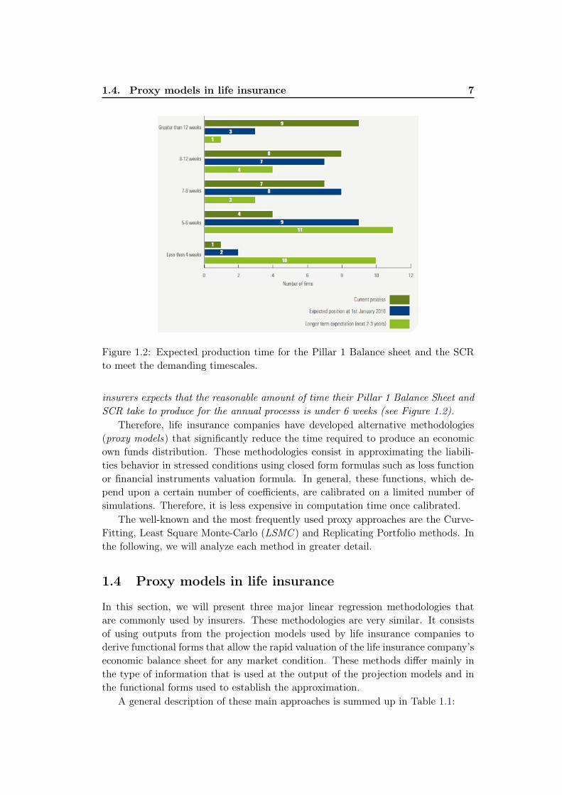
Figure 1.2: Expected production time for the Pillar 1 Balance sheet and the SCRto meet the demanding timescales.
insurers expects that the reasonable amount of time their Pillar 1 Balance Sheet andSCR take to produce for the annual processs is under 6 weeks (see Figure 1.2).
Therefore, life insurance companies have developed alternative methodologies(proxy models) that significantly reduce the time required to produce an economicown funds distribution. These methodologies consist in approximating the liabili-ties behavior in stressed conditions using closed form formulas such as loss functionor financial instruments valuation formula. In general, these functions, which de-pend upon a certain number of coefficients, are calibrated on a limited number ofsimulations. Therefore, it is less expensive in computation time once calibrated.
The well-known and the most frequently used proxy approaches are the Curve-Fitting, Least Square Monte-Carlo (LSMC ) and Replicating Portfolio methods. Inthe following, we will analyze each method in greater detail.
1.4 Proxy models in life insurance
In this section, we will present three major linear regression methodologies thatare commonly used by insurers. These methodologies are very similar. It consistsof using outputs from the projection models used by life insurance companies toderive functional forms that allow the rapid valuation of the life insurance company’seconomic balance sheet for any market condition. These methods differ mainly inthe type of information that is used at the output of the projection models and inthe functional forms used to establish the approximation.
A general description of these main approaches is summed up in Table 1.1:

8 Chapter 1. Introduction
Polynomial functions
LSMC Curve fitting Replicating portfolios
Cover all risks +++ +++ +Accuracy ++ ++ +Objectivity ++ + +
In line with market practice + ++ ++Implementation time and costs + ++ -Less Business-as-usual effort +++ + +required to perform runs
Table 1.1: Benchmark on the principle existing methods to calculate the SCR
1.4.1 Curve-Fitting
This methodology consists of constructing the best parametric form (linear combi-nation of analytic functions of real world risk factors) from a limited number of realworld scenarios for which a very precise valuation was performed. This parametriccurve thus passes through the calibration points (equality between the value of theparametric form and the value calculated within the projection model). To thatend each interpolation points must be estimated with an extremely high precision,which demands many simulations to improve the convergence rate. Therefore, thedisadvantages of this approach are that the data points must be carefully selectedby expert judgements and the number of interpolation points is really limited bysimulation time for each point [66].
To ensure that the estimator well replicate the economic own funds function,out of sample scenarios are used. The value of the parametric form is then com-pared with the value calculated within the projection model for these out of samplescenarios.
The criticisms relating to this methodology mainly concern its precision at thetail end. It is indeed necessary to ensure that there are enough extreme scenarios atthe tail end to ensure that the effects of non-linearity at the level of the liabilitiesin this area is correctly anticipated.
1.4.2 Least Square Monte-Carlo
The Least Square Monte-Carlo (LSMC) method was introduced by Longstaff andSchwartz [78] in order to evaluate American Bermudan options. The difficulty ofvaluing these options lies in the calculation of a retrograde algorithm based on theevaluation at each iteration of a conditional expectation. To avoid the need fornested simulations to calculate the conditional expectation at each date, Longstaffand Schwartz use an approximation to calculate this conditional expectation.

1.4. Proxy models in life insurance 9
Figure 1.3: Illustration of the curve-fitting estimation method.
Bermudan options valuation
We place ourselves in a probability space (Ω,F ,P), over a period of time [0, T ], wherethe sample space Ω is the set of possible realizations, F is the set of events containingthe information available at each date t, F = Ft; t ∈ [0, T ] with Fs ⊆ Ft for everys ≤ t, P is the historical probability. It is assumed that there is no arbitrageopportunity on the market, this implies that there is a risk-neutral probability Qequivalent to P.
American options can be exercised on specific dates between 0 and T , where T isthe expiry date of the option, we denote these exercise dates 0 < t1 ≤ · · · ≤ tN = T
with tk = kTN , ∆t = tk+1 − tk. The theoretical value of a Bermudan option under
risk-neutral probability is given by
V0 = supτ∈T
EQ [Zτe−rτ ]where τ∗ is a stopping time taking the values in T = t1, . . . , tN and Zt is thepayoff at time t.
To solve this problem, a dynamic programming method is used. The algorithmis written as follows:
VtN = ZTVtk = max
(Ztk ,EQ [e−r∆tVtk+1
| Ftk])
We adopt the convention that there is no early exercise opportunity at time 0,hence Z0 = 0. The terminal value ZT is known and the algorithm is reiteratedto determine V0. The delicate step of this algorithm is the computation of theconditional expectation (called value function), Longstaff and Schwartz propose anapproximation for this conditional expectation based on the least squares method.

10 Chapter 1. Introduction
We are interested here in derivative products whose payoffs are random variablesbelonging to the L2 (Ω,F ,Q) space, which is a Hilbert space. We know that theconditional expectation corresponds to the orthogonal projection on the Hilbertspace and is then the unique solution of the following minimization problem
EQ [X | F ] = arg minZ∈L2(Ω,F ,Q)
EQ [(X − Z)2]
(1.2)
The calculation of the value function is based on this characterization of the con-ditional expectation. Let S be the underlying of the option, Ft is the filtrationgenerated by S, which is a Markov process. Assume that we know how to simulatethe trajectories of the underlying under Q, so we have at each moment tk the Msimulated values Smtk , m = 1, . . . ,M .
Denote EQ [e−r∆tVtk+1| Ftk
]= EQ [e−r∆tVtk+1
| Stk]
= f(Stk). By consideringan orthonormal basis of our Hilbert space, the condition expectation can then beapproximated by a finite linear combination of this base that minimizes the criterionof conditional expectation (1.2). Given the basic functions pj, ∀j = 1, . . . , L, wethen look for the coefficients α∗j,k, solution of the least-squares problem:
α∗j,k = arg minαj,k
1
M
M∑m=1
e−r∆tV mtk+1−
L∑j=1
αj,kpj(Smtk)2
By replacing the optimal coefficients in the linear combination of the basic functions,we obtain an approximation of the value function for each trajectory m and at eachmoment tk:
EQ [e−r∆tVtk+1| Ftk
](m) ≈L∑j=1
α∗j,kpj(Smtk)
The following proposition provides a necessary and sufficient condition for theexistence of an optimal stopping time and characterizes the smallest optimal stop-ping time.
Proposition 1. There exists a stopping time τ∗ ∈ T such that EQ [Zτ∗e−rτ∗] =
supτ∈T EQ [Zτe−rτ ] if and only if Q(τ0 <∞) = 1, where
τ0 = inft ∈ T | Vt = Zt
The stopping time τ0 is then the smallest optimal stopping time.
This corresponds to the corollary 1.3.2 in [74]. By comparing the value of theimmediate exercise with the value function at each time step and for each trajectory,we are able to choose the optimal moment to exercise the option. We can nowdetermine the option price by taking the average of the discounted cash flows on eachtrajectories. Noting τ∗m the optimal stopping time corresponding to the trajectorym, we have:
V0 =1
M
M∑m=1
e−rτ∗mV
(m)τ∗m
.
1.4. Proxy models in life insurance 11
1.4.2.1 Application in Life Insurance
The application in Insurance of the LSMC method is based on the fact that the ownfund can be expressed as the expectation under the risk-neutral probability of thediscounted value of future profits conditional on the projection of the balance sheetin the "real world" universe (see, for instance, [7, 67,68,105,109]).
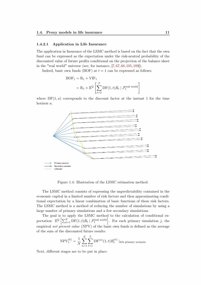
Indeed, basic own funds (BOF) at t = 1 can be expressed as follows:
BOF1 = R1 + VIF1
= R1 + EQ
[T∑t=2
DF(1, t)Rt | F real world1
]where DF(1, u) corresponds to the discount factor at the instant 1 for the timehorizon u.
Figure 1.4: Illustration of the LSMC estimation method.
The LSMC method consists of expressing the unpredictability contained in theeconomic capital in a limited number of risk factors and then approximating condi-tional expectation by a linear combination of basic functions of these risk factors.The LSMC method is a method of reducing the number of simulations by using alarge number of primary simulations and a few secondary simulations.
The goal is to apply the LSMC method to the calculation of conditional ex-pectation: EQ
[∑Tt=1 DF(1, t)Rt | F real world
1
]. For each primary simulation j, the
empirical net present value (NPV) of the basic own funds is defined as the averageof the sum of the discounted future results:
NPV(k)1 =
1
N
N∑n=1
T∑t=1
DF(n)(1, t)R(n)t |kth primary scenario
Next, different stages are to be put in place:

12 Chapter 1. Introduction
• Assume that each primary scenario can be synthesized at time t, using d riskfactors (x1, . . . , xd).
• Approximation of BOF1 by a finite linear combination of basic functions
pjj=1,...,L of these risk factors: BOF(k)
1 =∑J
j=1 βjpj
(x
(k)1 , . . . , x
(k)d
).
• Calculation of the empirical NPV(k)1 for each primary simulation k.
• Determination of optimal coefficients using the generalized least squaresmethod:
β = arg minβ∈RJ
K∑k=1
NPV(k)1 −
J∑j=1
βjpj
(x
(k)1 , . . . , x
(k)d
)• Calculation of BOF1 by replacing β by β.
The algorithm makes it possible to avoid the nested simulations since the conditionalexpectation is directly calibrated on the empirical NPV of the basic own funds viasome secondary simulations.
1.4.3 Replicating Portfolios
A replicating portfolio of a set of liabilities is:
• a portfolio of standard financial instruments
• that has the same market consistent value as the liabilities, and
• that has similar market consistent value sensitivities to market risks drivers.
This proxy model builds a representation of the liabilities using vanilla financialinstruments. This is a reasonably quick solution, relying mainly on the abilityto represent exotic financial instruments (insurance) using only vanilla financialinstruments. This representation is built on the projection system results. It is thencombined with a line-by-line model of the assets to build a synthetic economic viewof the market consistent balance sheet. The full range of initial market conditionscan then be run in a very timely manner. This methodology has the advantage thatit gives an understandable structure of the liabilities, which itself can
• provide insight into the business and into the financial risks
• help design hedging strategies
• help focus the calibration of the ESG to the most relevant financial instruments
• enable to challenge the results of the projection system.

1.4. Proxy models in life insurance 13
If liabilities are independent from the backing assets and from the financial market,the liabilities cash flows are certain and each cash-flow can be represented by a zero-coupon bond of the same maturity and same amount. One scenario is sufficientto project all liabilities cash-flows and to determine the equivalent zero couponbonds. However, the replicating portfolio can also be determined using the presentvalue of cash flows under different scenarios. Therefore, for Property and Casualty(P&C) and life non-participating line of businesses, the cash flows can be perfectlyreplicated whatever the market conditions are. As a result, the replicating portfoliois as accurate as the projection system.
Even if liabilities do depend on the backing assets performance, for examplethrough a profit sharing mechanism, it is possible to represent the liabilities usingfinancial instruments. Let us consider as an example a traditional savings productwith a guaranteed rate, and a guaranteed surrender value. The detail of the surren-der modelling will be presented later. Here we briefly summarize the behaviour ofthe policyholders:
• If market rates increase above the policy guaranteed rate, the lapses will in-crease the policyholders will take advantage of the guaranteed surrender value(higher than the market value of the values) and re-invest at market rates; theresulting liability cash-flows can be represented by payer swaptions;
• If market rates decrease below the policy guaranteed rate, the lapses willdecrease: the policyholders will take advantage of the guaranteed rate: theresulting cash-flows can be represented by receiver swaptions.
Not all policyholders will act as described-but at a portfolio level, it is possible torepresent the liabilities as a combination of zero-coupon (base guarantee), receiverswaptions (lower lapses with lower rates), and payer swaptions (higher lapses atguaranteed value with higher rates). The strikes of the swaptions will depend onthe lapse function.
However, it should be noted that it is often difficult to match complex liabilitieswell with replicating assets because the required instruments are not available in themarket (see, for instance, [15,69,82,114]).Replicating portfolios only cover financialand credit (spread) risk and therefore polynomial loss functions are still needed forall other risks.
1.4.3.1 Determination of a replicating portfolio
This step is meant to find a set of financial instruments which achieves the bestmatch of the market consistent values and sensitivities. In this section, we willhowever get into the details of this process since it goes beyond the scope of ourobjectives. In general, it will be an iterative process of:
1. Finding a candidate replicating portfolio,
2. Assessing its quality,

14 Chapter 1. Introduction
3. Repeating until predefined quality criteria are met.
The very first step is to define a list of candidate financial instruments. Insuranceliability features will link to different types of financial instruments or to differentcharacteristics of the financial instruments. It is therefore important to understandthe features of the liability being replicated to retain relevant instruments. In mostcases, the instruments will be a combination of: zero-coupons of different maturitiesrepresenting the expected premiums to be received, claims to be paid, guaranteesprovided; receiver and payer swaptions of different maturities, tenor and strikes,representing the options given to policyholders; puts or calls on equities of diiferentmaturities and strikes representing the profit-sharing given to policyholders.
The second step consists in finding the weights of all candidate instruments thatwill make the replicating portfolios closest to the liabilities. To this end we calculatethe present values (PV) of the liabilities cash-flows resulting from a set of scenariosrun through the projection system. We then define a distance on the present valueof cash-flows vector space, which enables a direct resolution of the minimization toobtain the optimal weighting coefficients. Namely, denote by ωkKk=1 the weightingcoefficients associate to K candidate instruments, we have
ω∗1, . . . , ω∗J = arg min
ω1,...,ωJ
N∑n=1
[T∑t=1
(K∑k=1
ωkCF(n)RP,k(t)− CF(n)
L,k(t)
)DF(n)(0, t)
]2
(1.3)
In simple cases, representations of liabilities can be built using those financial in-struments leading to high quality results for the calculation of the SCR.
1.4.4 Acceleration algorithm
Devineau and Loisel [30] develop an acceleration algorithm for the Nested Simulationmethod described previously. This algorithm aims to reduce the overall number ofprimary simulations to be carried out. The key idea of this method is to select themost adverse trajectories in terms of solvency according to the chosen risk factorsand to do the simulations only along these adverse trajectories. To sum up, theacceleration algorithm is implemented in three key steps:
1. Extract the elementary risk factors that have the most impact on the items ofthe balance sheet for each primary simulation.
2. Define a fixed threshold confidence region: only primary simulations for whichrisk factors are outside the confidence region are performed.
3. Make iterations on the threshold of the region in order to integrate each stepa number of additional points.
The basic idea behind this method is similar to the one of Lan et al. [72], whodescribe a screening procedure for expected shortfall based on nested simulations.The main advantage of this method is that it considerably reduces the calculation
1.5. Error quantification for internal modeling in life insurance 15
times and the necessary resources. However, the speed of the algorithm rapidlydecreases when the number of risk factors increases. Hence, only the risks havingsignificant impacts on the portfolio are selected for the solvency assessment. Thistechnique focuses on estimating economic capital and it is hard to apply to theportfolio risk management. Therefore, we observe that this method is rarely usedin practice.
1.5 Error quantification for internal modeling in life in-surance
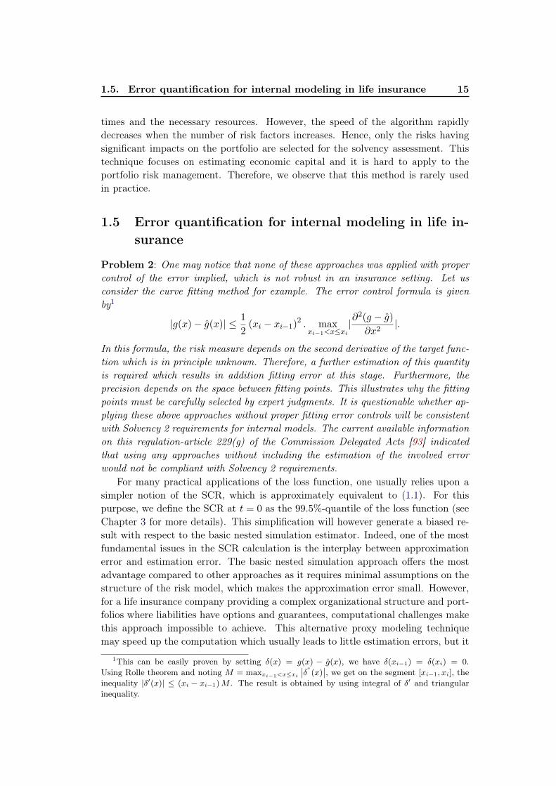
Problem 2: One may notice that none of these approaches was applied with propercontrol of the error implied, which is not robust in an insurance setting. Let usconsider the curve fitting method for example. The error control formula is givenby1
|g(x)− g(x)| ≤ 1
2(xi − xi−1)2 . max
xi−1<x≤xi|∂
2(g − g)
∂x2|.
In this formula, the risk measure depends on the second derivative of the target func-tion which is in principle unknown. Therefore, a further estimation of this quantityis required which results in addition fitting error at this stage. Furthermore, theprecision depends on the space between fitting points. This illustrates why the fittingpoints must be carefully selected by expert judgments. It is questionable whether ap-plying these above approaches without proper fitting error controls will be consistentwith Solvency 2 requirements for internal models. The current available informationon this regulation-article 229(g) of the Commission Delegated Acts [93] indicatedthat using any approaches without including the estimation of the involved errorwould not be compliant with Solvency 2 requirements.
For many practical applications of the loss function, one usually relies upon asimpler notion of the SCR, which is approximately equivalent to (1.1). For thispurpose, we define the SCR at t = 0 as the 99.5%-quantile of the loss function (seeChapter 3 for more details). This simplification will however generate a biased re-sult with respect to the basic nested simulation estimator. Indeed, one of the mostfundamental issues in the SCR calculation is the interplay between approximationerror and estimation error. The basic nested simulation approach offers the mostadvantage compared to other approaches as it requires minimal assumptions on thestructure of the risk model, which makes the approximation error small. However,for a life insurance company providing a complex organizational structure and port-folios where liabilities have options and guarantees, computational challenges makethis approach impossible to achieve. This alternative proxy modeling techniquemay speed up the computation which usually leads to little estimation errors, but it
1This can be easily proven by setting δ(x) = g(x) − g(x), we have δ(xi−1) = δ(xi) = 0.Using Rolle theorem and noting M = maxxi−1<x≤xi
∣∣δ”(x)∣∣, we get on the segment [xi−1, xi], the
inequality |δ′(x)| ≤ (xi − xi−1)M . The result is obtained by using integral of δ′ and triangularinequality.

16 Chapter 1. Introduction
will generate approximation errors as we impose additional assumptions. When thenumber of risk drivers increases, these approximation errors may have a substantialimpact on the estimated capital requirement. We will keep for further research toquantify the approximation errors in high dimensional settings. Finally, to ensurethat these approximation errors in low dimensional settings are relatively small andacceptable, we prepare the box-whisker plot to see how good the approximation is.
1.6 Application of Extreme Value Theory to SolvencyCapital Requirement estimation
One of the difficulties of SCR estimation is that one must evaluate quantities thatdepend on the tail of distribution, for which, almost by definition, one does nothave observations or at least one has only very few observations. Recall that thesimulation-based capital estimates are carried out as follows:
1. Generate real-world economic scenarios for all risk drivers affecting the balancesheet over one year,
2. Revalue the balance sheet under each real-world scenario (by using, for exam-ple, Monte Carlo (nested simulation), Replicating Portfolio, etc.),
3. Estimate the statistics of interest.
However, there exists many sources of uncertainty in this process. Namely, it de-pends on the choice of economic scenario generator models and their calibration,the liability model assumptions (e.g. dynamic lapse rules), as well as the choice ofscenarios sampled (i.e. choice of real world ESG random number seed). Usually, aninsurer will rely on expert judgement to define economic scenario generator modelsand liability model assumptions. Therefore, the first two sources of uncertainty arebeyond the scope of our work and we are particularly interested in the last source ofuncertainty, which is simply a statistical uncertainty. We wonder if we can estimatethis statistical uncertainty. If so, how can we reduce the amount of statistical un-certainty? In our work, we will address these questions using a statistical techniqueknown as Extreme Value Theory (EVT).
Recall that Extreme Value Theory tells us something about the shape of thedistribution in the tail. The standard approaches for describing the extreme eventsof a stationary time series are the block maxima approach (which models the maximaof a set of blocks dividing the series) and the Peak-over-Threshold (POT) approach(which focuses on exceedances over a fixed high threshold). The POT method hasthe advantage of being more flexible in modeling data, because more data pointsare incorporated (see Chapter 4.1 for more details). Hence, the method we use inour study is the POT method.
According to this method, the distribution of liability value beyond some thresh-old is approximated as a Generalized Pareto distribution (GPD), which is parame-terized by 2 parameters: scale σ and tail-index γ. Therefore, we can estimate the

1.7. Contributions and structure of the thesis 17
tail of the distribution by picking a threshold and fitting the 2 parameters of theGeneralized Pareto distribution to values in excess of the threshold.
In the context of financial and actuarial modeling, the observations very oftendepend on the other parameters, such as business line, risk profile, seniority, etc.However, all these studies assume that the tail-index is constant regardless of thesevariables. Many recent studies, for example [23,117], emphasized that the tail-indexcould be function of these explanatory variables. But none of the previously men-tioned studies provide a way to estimate the tail-index parameter conditionally tothese variables. As far as we can tell, in the context of financial and actuarial mod-eling, only three studies have been undertaken to provide methods to estimate thetail-index parameter conditionally to covariates. Beirlant and Goegebeur [9] proposea local polynomial estimator in the case of a one-dimensional covariate. When thedimension of the covariate increases, this method becomes less effective since theconvergence rate of the estimator decreases rapidly. To improve the performanceof the estimator, a solution would be to increase the size of data, but this wouldbe problematic in practice since the database could not be easily enlarged. Then,Chavez-Demoulin et al. [22] propose an additive structure with spline smoothing toestimate the relationship between the GDP parameters and covariates. Recently,Heuchenne et al. [52] approach suggests a semi-parametric methodology to estimatethe tail-index parameter of a GPD.
In practice, many financial and actuarial data modeling problem may dependupon several explanatory variables, which might make direct tail-index parameterestimation less accurate, or even impossible. However, it does not mean that allof these explanatory variables have more or less the same impact on the result.For example, Chernobai et al. [23] investigate the relation between frequency ofoperational loss events and firm-specific variables (market value of equity, firm age,cash holding ratio, etc.) as well as macroeconomic variables. They find a strongdependence between frequency and firm specific variables, but only weaker resultswith respect to the macroeconomic variables. This remark could also be true for thecapital requirement. Therefore, it exists therefore a real need for companies to map,model and measure those risks to take proper hedging action. One technique toreduce dimension is sparse group lasso, which was introduced by Simon et al. [100].Motivated both by the advances about the work of Chavez-Demoulin et al. [22]and the sparse group lasso method, we investigate a variable-selecting method toestimate the tail-index parameter conditionally to covariates.
1.7 Contributions and structure of the thesis
1.7.1 Contribution to the company
For PwC, the interest of sponsoring this PhD study is undeniable. Indeed, thisproject aims to perform a bibliographic research on recent scientific works concerningthe actuarial finance, to know and understand some techniques used by insurers. andto be able to propose new commercial offers which can stand out competition. In

18 Chapter 1. Introduction
this sense, I think that this last objective was correctly achieved to the extent thatmy first research work that I have provided has made it possible to quantify andcontrol the errors in the actuarial calculation engines.
Following the work carried out with clients in the context of either auditor’smandates or consultancy assignments, I have also established a benchmark of marketpractices concerning the implementation of Pillar I of the Solvency II Directive withrespect to the saving contracts in euros (see Figure 1.5 in French).
Besides, I developed and put in place (i) a cross-asset Economic Scenarios Gen-erator and (ii) an actuarial ALM simulator in life insurance. The ESG enabblesus to simulate future states of the global economy and financial markets. It usesadvanced modeling and estimation technology to produce empirically validated, re-alistic economic scenarios which are used as inputs to the ALM simulator. Thesenumerical tools result in numerous important contract wins for PwC. In the future,PwC would like to commercialize these numerical tools and present this work toclients. An overall introduction of these tools are given in Appendix A and B.
1.7.2 Methodological contributions
The works presented in this thesis attempt to bring a set of contributions to theperformance of internal modeling in life insurance by applying advanced statisticaltechniques, while being easily implementable and numerically stable. In each of thesimulation studies, We prove theoretical properties for the methods put in place,and we also show that these are relevant in practice and at least match the existingprocedures. The results obtained allow us to consider different lines of research.
Error quantification for internal modeling in life insurance
In this work, I develop a new fitting methodology for estimating the SCR (Problem1) and a formula for controlling the deviation of the target SCR from its estimate(Problem 2). The new method operates in the following way.
We proposed to calculate the SCR as the 99.5%-quantile of the loss function (seeSection 3.3.2 for the definition of the loss function), i.e.
SCR = q99.5%(φ) (1.4)
The loss function φ(x1, . . . , xd) is then decomposed into the stand-alone loss func-tions φj(xj)j=1,...,d and the excess loss function φ1d(x1, . . . , xd) as follows:
φ(x1, . . . , xd) =d∑j=1
φj(xj) + φ1d (x1, . . . , xd) . (1.5)
Next we apply the Bayesian penalized spline regression technique to estimate eachfunctional component. For later use, we denote by φ the estimate of φ.
The SCR can be estimated by SCR = q99.5%
(φ)its empirical 99.5th-percentile
derived from φ. In this stage, φ ≡ φ(X) is a random variable with X = (X1, . . . , Xd)

1.7. Contributions and structure of the thesis 19
Figure 1.5: Benchmark Pillar 1 of Solvency II (Certain information are confidential,and thus will not be mentioned in this table).

20 Chapter 1. Introduction

1.7. Contributions and structure of the thesis 21

22 Chapter 1. Introduction
the realistic random market state or the primary simulation state whose marginaldistribution is PX . Let fφ denote the density function of φ(X).
To control the probability of deviation of the target SCR from its estimate, wewill need certain conditions to make the theory work. First of all, it is important toclarify that as will be seen below, the resulting confidence band will not incorporatethe approximation error from the choice of the regression function.
Let us introduce some notation, definitions that will be used in the sequel. Wedefine the (L,Ω)-Lipschitz class of functions, denoted Σ(L,Ω), as the set of functiong : Ω→ R satisfy, for any x, x′ ∈ Rd, the inequality:
|g(x′)− g(x)| ≤ L‖x′ − x‖
with Ω ⊂ Rd and ‖x‖ , (x21 + · · · + x2
d)1/2. Let r > 0. We define B(a, r) =
x ∈ Rd | ‖a − x‖ ≤ r. We denote by Vφ = x ∈ Rd | φ(x) = q99.5%(φ) andVφ = x ∈ Rd | φ(x) = q99.5%(φ) the closed set of the 99.5th-percentile scenariosfor φ and φ respectively.
Let Γ denote the available sampling budget used to calibrate φ. Based on thework of Aerts et al. ( [2]), it is straightforward to deduce that for λφj (Γ) and λhJ (Γ)
tending to 0, the estimate φ converges in mean square to φ as Γ→∞. Furthermore,by Markov’s inequality, convergence in mean square of φ leads to the convergencein probability of φ(x) to φ(x) for every x ∈ Rd. This implies that for every x∗ ∈ Vφ,there exists a random sequence x∗(Γ) ∈ Vφ converges in probability to x∗.
Introduce now three assumptions on φ, φ and x∗(Γ) that will be used in the laststep:
ASSUMPTION 1: Suppose that φ ∈ Σ(L,Ω) where L > 0 and Ω(⊃ Vφ) is anopen subset of Rd.
ASSUMPTION 2: For any x∗ ∈ Vφ and r > 0, there exists two positive constantsξ(r, d), γ(r, d) such that
P(‖x∗ − x∗(Γ)‖ > r
)≤ ξ(r, d)Γ−γ(r,d)
for large enough Γ.ASSUMPTION 3: For any choice of x∗ ∈ Vφ and α ∈ (0, 1), there exists two
positive constants r(Γ) and ∆(α,Γ), with r(Γ)Γ→∞−−−→ 0, such that
P(| φ(x)− φ(x) |> ∆(α,Γ)
)≤ 1− (1− α)
d(d+3)2 , ∀x ∈ B(x∗, r(Γ))
for large enough Γ.
• SCR estimation error control: In the following, we denote by N1 the numberof the primary simulations. Note that∣∣∣SCR− SCR∣∣∣ ≤ ∣∣∣q99.5%
(φ)− q99.5%
(φ)∣∣∣+
∣∣∣q99.5%
(φ)− q99.5% (φ)
∣∣∣ (1.6)
The first term on the right-hand side corresponds to the numerical error sincewe appeal the empirical percentile to estimate the SCR and the second term

1.7. Contributions and structure of the thesis 23
represents the model error. Note that the numerical error depends not only onthe empirical assessment q99.5 but also on the fitting quality φ. To value thisnumerical error, we apply the Theorem in Appendix D.8. Namely, we have
P
∣∣∣q99.5%
(φ)− q99.5%
(φ)∣∣∣ > zα/2
0.07√N1fφ(q99.5%
(φ)
)
→ α (1.7)
as N1 →∞. In the previous expression, the distribution function fφ and the
evaluated point q99.5%
(φ)are however unknown and will be then replaced by
their estimators. Regarding the second term, by using Assumptions (1-3), weobtain the asymptotic probability of deviation of q99.5%
(φ)
from q99.5% (φ)
having the form:
P(∣∣∣q99.5%
(φ)− q99.5% (φ)
∣∣∣ > ∆(α,Γ) + Lr∗)≤[1− (1− α)
d(d+3)2
]+ ξ(r∗, d)Γ−γ(r∗,d) (1.8)
where r∗ ≡ r(Γ). The derivation of this result can be found in Appendix D.6.Combing the equations (1.7) and (1.8) leads to the control of the probabilityof deviation of SCR from SCR.
The confidence interval ∆(α,Γ)+Lr∗ is however an issue as it involves the unknownparameters ∆(α,Γ), L and r∗. In the following, we suggest a method to estimatethese parameters in practice.
In order to estimate the Lipschitz constant, we find the supremum of all slopes|φ(x)−φ(x′)|/‖x−x‖ for distinct points x and x′ within the 99.5th-percentile region.We call x∗ the empirical 99.5th-percentile scenario, i.e. φ(x∗) = q99.5%
(φ). The
parameter ∆(α,Γ) will be then replaced by ∆(α,Γ) =∑d
j=1 ∆(x∗)j,α +
∑J ∆
(x∗)J,α . To
estimate the parameter r∗, we seek the maximum radius r∗ such that for everyx(ν) ∈ B(x∗, r∗), the confidence intervals
∑dj=1 ∆
(ν)j,α+
∑J ∆
(ν)J,α are close to ∆(α,Γ).
On the right-hand side of the inequality (1.8), as the true value of ξ(r∗, d) andγ(r∗, d) are unknown, it is not possible to have a direct access to the upper boundof the probability. In practice, a large number of Γ is necessary so that the term[1− (1− α)d(d+3)/2
]becomes preponderant compared to ξ(r∗, d)Γ−γ(r∗,d).
For many practical applications of the loss function, one usually relies upon asimpler notion of the SCR, which is approximately equivalent to Eq. 1.1. Thissimplification will however generate a biased result with respect to the basic nestedsimulation estimator. Indeed, one of the most fundamental issues in the SCR cal-culation is the interplay between approximation error and estimation error. Thebasic nested simulation approach offers the most advantage compared to other ap-proaches as it requires minimal assumptions on the structure of the risk model,which makes the approximation error null. However, for a life insurance companyproviding a complex organizational structure and portfolios where liabilities haveoptions and guarantees, computational challenges make this approach impossible to
24 Chapter 1. Introduction
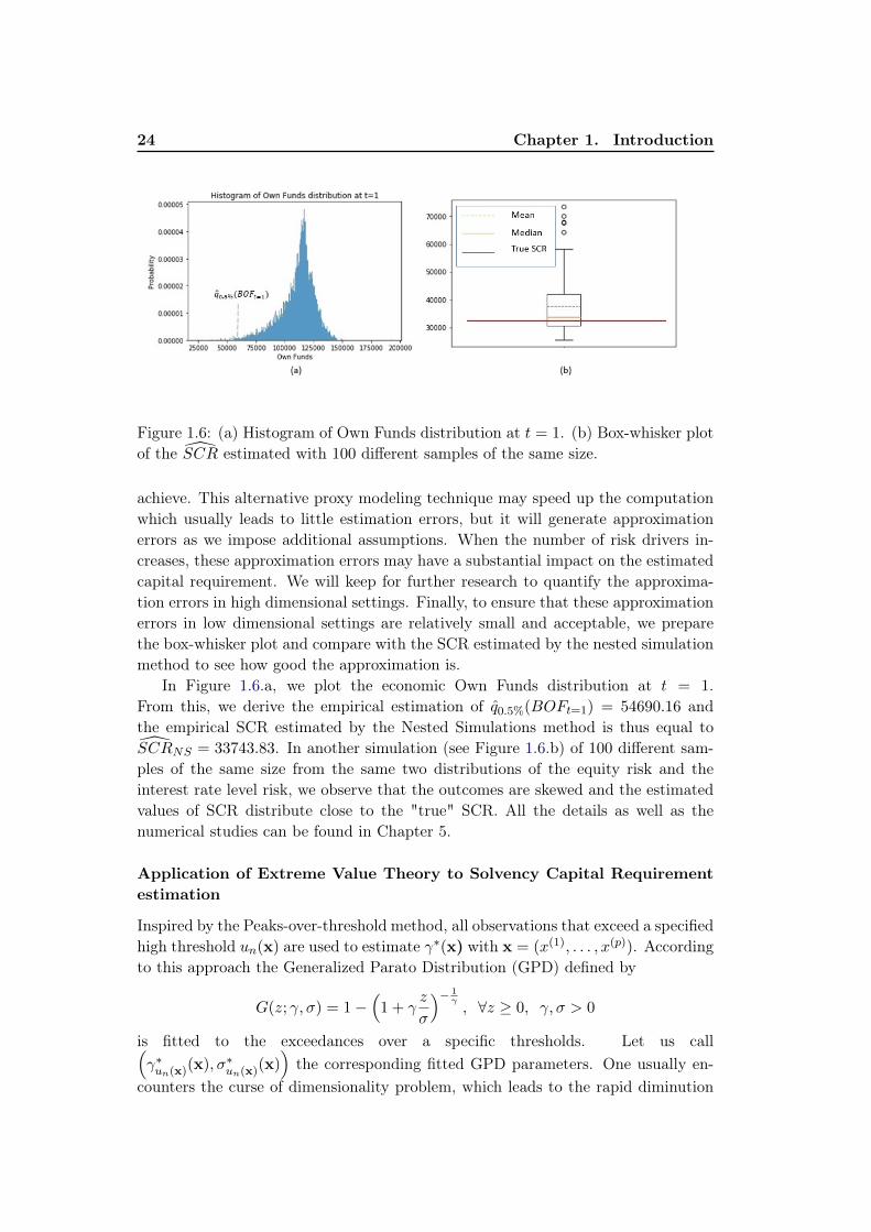
Figure 1.6: (a) Histogram of Own Funds distribution at t = 1. (b) Box-whisker plotof the SCR estimated with 100 different samples of the same size.
achieve. This alternative proxy modeling technique may speed up the computationwhich usually leads to little estimation errors, but it will generate approximationerrors as we impose additional assumptions. When the number of risk drivers in-creases, these approximation errors may have a substantial impact on the estimatedcapital requirement. We will keep for further research to quantify the approxima-tion errors in high dimensional settings. Finally, to ensure that these approximationerrors in low dimensional settings are relatively small and acceptable, we preparethe box-whisker plot and compare with the SCR estimated by the nested simulationmethod to see how good the approximation is.
In Figure 1.6.a, we plot the economic Own Funds distribution at t = 1.From this, we derive the empirical estimation of q0.5%(BOFt=1) = 54690.16 andthe empirical SCR estimated by the Nested Simulations method is thus equal toSCRNS = 33743.83. In another simulation (see Figure 1.6.b) of 100 different sam-ples of the same size from the same two distributions of the equity risk and theinterest rate level risk, we observe that the outcomes are skewed and the estimatedvalues of SCR distribute close to the "true" SCR. All the details as well as thenumerical studies can be found in Chapter 5.
Application of Extreme Value Theory to Solvency Capital Requirementestimation
Inspired by the Peaks-over-threshold method, all observations that exceed a specifiedhigh threshold un(x) are used to estimate γ∗(x) with x = (x(1), . . . , x(p)). Accordingto this approach the Generalized Parato Distribution (GPD) defined by
G(z; γ, σ) = 1−(
1 + γz
σ
)− 1γ, ∀z ≥ 0, γ, σ > 0
is fitted to the exceedances over a specific thresholds. Let us call(γ∗un(x)(x), σ∗un(x)(x)
)the corresponding fitted GPD parameters. One usually en-
counters the curse of dimensionality problem, which leads to the rapid diminution

1.7. Contributions and structure of the thesis 25
in convergence rate, when the covariate is high dimensional. To overcome this dif-ficulty, we assume that γ∗un(x)(x) and σ∗un(x)(x) are approximated by a generalizedadditive model as follows
γp,∞(x) = exp
γ0 +
p∑j=1
γj(x(j))
σp,∞(x) = exp
σ0 +
p∑j=1
σj(x(j))
where each additive function γj(·), σj(·) belongs to the Sobolev space of continuouslydifferentiable functions. In order to ensure the identification we assume that forevery j = 1, . . . , p the additive functions γj , σj are centered, i.e.
n∑i=1
γj
(x
(j)i
)= 0,
n∑i=1
σj
(x
(j)i
)= 0. (1.9)
These statistical models are still nonparametric and the estimation therefore a prob-lem of infinite dimension. We make it finite by expanding each additive functionalcomponents in natural cubic spline (NCS) bases with a reasonable amount of knotsKj for j = 1, ..., p. Thus, we parametrize
γj(·) =
Kj∑k=2
θj,k
(hj,k(·)−
1
n
n∑i=1
hj,k
(x
(j)i
)), σj(·) =
Kj∑k=2
θ′j,k
(hj,k(·)−
1
n
n∑i=1
hj,k
(x
(j)i
))
where hj,k : R→ R+ is the natural cubic spline basis function constructed on the setof the predefined interior knots ξ(j)
1 , . . . , ξ(j)Kj satisfying ξ(j)
1 ≤ · · · ≤ ξ(j)Kj
. Clearly,this parametrization of the functional components (γj(·), σj(·)) verifies the centeringconditions given in (1.9). To simplify our notation, let us define
hj,k(·) =
(hj,k(·)−
1
n
n∑i=1
hj,k
(x
(j)i
)), ∀j = 1, . . . , p, ∀k = 1, . . . ,Kj .
In the following, we denote by β0 and θ0 the intercept term instead of γ0 and σ0
to synchronize the notation with the coefficients θj,k, θ′j,k as presented previously.
Finally, our statistical model is defined as
γ(x) = exp
θ0 +
p∑j=1
Kj∑k=2
θj,khj,k
(x(j))
σ(x) = exp
θ′0 +
p∑j=1
Kj∑k=2
θ′j,khj,k
(x(j))
To sum up, the following diagram sets out the whole approximation scheme:Next, we denote by ϕ =
(θ0,θ
T , θ′0,θ
′,T)
the entire parameter vector where

26 Chapter 1. Introduction
θ =(θT1 , . . . ,θ
Tp
)T , θ′ =(θ′,T1 , . . . ,θ
′,Tp
)Twith θj =
(θj,2, . . . , θj,Kj
)T and
θ′j =
(θ′j,2, . . . ,θ
′j,Kj
)Tfor every j = 1, . . . , p. Clearly, the parameter vector ϕ
can be structured into groups G0,G1, . . . ,Gp and G0, G1, . . . , Gp. Each of the groupsis defined in the following way:
θ0 = ϕG0 , θj = ϕGj , θ′0 = ϕG0
, θ′j = ϕGj , ∀j = 1, . . . , p.
Under this notation, our models can be rewritten as
γ(x|ϕ) = exp
p∑j=0
ϕGj hGj
(x(j))
σ(x|ϕ) = exp
p∑j=0
ϕGj hGj
(x(j))
with hG0(·) = hG0(·) = 1.
For the purpose of variable selection and eliminating perturbative effects withineach group, we suggest to use the sparse group lasso technique to estimate(γ(x|ϕ), σ(x|ϕ)). Namely, the regression model used to estimate (γ(x|ϕ), σ(x|ϕ))
is defined by
ϕ(un(·),λ,µ) = arg minϕ
Pnl(ϕ|un(·)) + pen (ϕ|λ,µ) . (1.10)
where
Pnl(ϕ|un(·)) = − 1
n
n∑i=1
log g (yi − un(xi); γ(xi|ϕ), σ(xi|ϕ)) I(yi ≥ un(xi)).
with yi a realisation of Yi and the penalty
pen (ϕ|λ,µ) = λ1
p∑j=1
√Gj‖ϕGj‖2+λ2
p∑j=1
‖ϕGj‖1+µ1
p∑j=1
√Gj‖ϕGj‖2+µ2
p∑j=1
‖ϕGj‖1
with Gj ≡ |Gj | = |Gj | the cardinality of the group Gj , as well as of the group Gj ,λ = (λ1, λ2)T ∈ R2
∗,+ and µ = (µ1, µ2)T ∈ R2∗,+. The algorithm used to solve the
equation (1.10) is summarized in Algorithm 1.A well-known drawback of l1-penalized estimators is the systematic shrinkage of
the large coefficients towards zero. This may give rise to a high bias in the resulting

1.7. Contributions and structure of the thesis 27
estimators and may affect the overall conclusion about the model. We then need torefit the model without any penalties on the select support
SG = (j, k)|ϕGj,k 6= 0, SG = (j, k)|ϕGj,k 6= 0.
Finally, we perform a numerical study with different settings (i.e. p = 2, 10 andn = 500, 5000) and compare the estimating performance of our methodology withan existing method proposed by Beirlant and Goegebeur [9]. Usually in many high-dimensional studies, the dimension of the data vectors p is comparable or may belarger than the sample size n. Hence, it is obvious that our setting with p = 10
can not be considered as high dimensional covariate. However, we realized that itbecomes computationally expensive in terms of running time required to performestimation when the dimensionality increases. Therefore, in this thesis, we limitourselves to the case p = 10. Surprisingly, we note that the proposed methodologyslightly outperforms even with p = 10. And we hope in the near future that we canreinforce our results with higher dimensionality.
1.7.3 Structure of the thesis
As can be seen, this thesis, which is constituted of two parts, is organized in sevenchapters:
- The first part deals with the error quantification problem for internal modelingin life insurance. It consists of four different chapters. Chap. 2, 3 and 4 are introduc-tory chapters. Chap. 2 and 3 present respectively our Economic Scenario Generator(ESG) and Asset-Liability Management (ALM) cash-flows simulator, which are themain tools used to value the economic balance sheet. Chap. 4 is a general pre-sentation: the statistical framework and the nonparametric estimation methods areintroduced. All these chapters will provide us fundamental elements to achieve ourfindings presented in Chap. 5.
- The second part deals with the application of Extreme Value Theory to Sol-vency Capital Requirement estimation when the covariate information is available.Especially, when the covariate are high dimensional, we face with the curse of dimen-sionality problem resulting in a decrease in fastest achievable rates of convergence ofregression function estimators toward their target curve. This problem refers to thephenomenon where the volume of covariate space increases so fast that the availabledata become sparse. In order to obtain a statistically sound and reliable result,the amount of data needed to support the result often grows exponentially withthe dimensionality, which is usually problematic in many practical applications. Toovercome this estimating problem, we propose a new methodology for effectivenessevaluation, which is described in Chap 4.
Publication
Duong, Q.D., Application of Bayesian penalized spline regression for internal mod-eling in life insurance. European Actuarial Journal 9, 67–107(2019).

28 Chapter 1. Introduction
Submitted paper
Duong, Q.D., Guilloux, A. and Lopez, O., Sparse group lasso additive modeling forPareto-type distributions. Submitted to Computational Statistics journal.

Chapter 2
Solvency II - Interpreting the keyprinciples of Pillar I
Contents2.1 History of capital requirements in the European insurance
industry . . . . . . . . . . . . . . . . . . . . . . . . . . . . . . . 292.1.1 Solvency I directive . . . . . . . . . . . . . . . . . . . . . . . 292.1.2 From Solvency I to Solvency II . . . . . . . . . . . . . . . . . 30
2.2 Implementation of Solvency II . . . . . . . . . . . . . . . . . 312.3 Pillar I . . . . . . . . . . . . . . . . . . . . . . . . . . . . . . . . 32
2.3.1 The quantitative requirements of Pillar 1 . . . . . . . . . . . 332.3.2 Standard Formula . . . . . . . . . . . . . . . . . . . . . . . . 352.3.3 Internal Model . . . . . . . . . . . . . . . . . . . . . . . . . . 38
2.1 History of capital requirements in the European in-surance industry
2.1.1 Solvency I directive
The first European regulations on minimum capital to be held date back to the1970s. In 1973 and 1979, two directives was published; one in the non-life insurancesector1 and one in the life insurance sector2. These impose for the first time Euro-pean insurers to build a layer of security in terms of own funds. In February 2002
the Solvency I directives were adopted. Recall that these directives had remainedbroadly close to the first European regulations.
The model developed under Solvency I to assess the solvency capital requirementis simple. According to Solvency I, the risk is either in provisions or in premiums.The calculation of the capital required is a so-called "factor-based" approach, whichmeans that the required capital is calculated as a fraction of the elements considered
1First Council Directive 73/239/EEC of 24 July 1973 on the coordination of laws, regulationsand administrative provisions relating to the taking-up and pursuit of the business of direct insur-ance other than life assurance
2First Council Directive 79/267/EEC of 5 March 1979 on the coordination of laws, regulationsand administrative provisions relating to the taking up and pursuit of the business of direct lifeassurance

30 Chapter 2. Solvency II - Interpreting the key principles of Pillar I
as risky on the balance sheet (technical provisions) or on the profit and loss account(premiums).
2.1.2 From Solvency I to Solvency II
Solvency I has the merit of being simple and can therefore be implemented at alower cost. In addition, the regulations allow a quick comparison of the resultsobtained for different companies. The approach is nevertheless not adequate forseveral reasons, which will be discussed later. It thus justified the initiation of thenew reform, called Solvency II project, hereinafter Solvency II for short.
Firstly, the level of technical provisions or the premium amounts are not inthemselves good indicators of risk, for several reasons:
1. The approach does not take into account the level of prudence of the insurerin its provisioning. For example, a prudent insurer, better endowed withtechnical provisions, must mobilize more capital than an insurer with lessprovision. Such a system therefore penalizes prudential.
2. The approach highlighted in Solvency I is based only on the liabilities balancesheet of insurance companies, while other risks should be considered, suchas asset risks, i.e. market and credit risks. In addition, the solvency capitalrequirements do not take into account, for example, the investment structureof the insurance company.
3. The risk reduction methods are also ignored: diversification between risks,risk transfer, asset-liability management, risk hedging instruments. The useof financial derivatives products, the use of reinsurance, the credit quality ofre-insurers, etc., should also influence the required solvency margin.
Secondly, the assets and liabilities are valued at historical cost (or book value).However, this valuation method does not reflect the risks and the real value of theassets and liabilities. Finally, the Solvency I regime can lead to systemic risks.In fact, by way of illustration, a compulsory pricing framework for all insurancecompanies exposes all these companies to the same risks of errors in tariffs. Tosum up, Solvency I does not adequately reflect the risk profile of each insurancecompanies concerned. These weaknesses justified the need for a regulatory reform.
The lessons learned from the years 2002 and 2003, during which the financialmarkets experienced a period of crisis, while at the same time putting the financialhealth of some insurance companies at a disadvantage, led the regulators to take areview of the risk valuation framework within the insurance industry. Since March2003, the European Commission, in collaboration with the member states, had beenworking on developing a single reference system aimed at better integrating risk intothe constraints imposed on insurers in order to ensure their ability to fulfill theircommitments. This is the Solvency II Project.

2.2. Implementation of Solvency II 31
2.2 Implementation of Solvency II
As one of the most crucial projects currently being carried out by the Commissionand the member states in the insurance sector, Solvency II consists in developinga novel, better risk-adjusted system for assessing the overall solvency of insurancecompanies. Namely, this system provides the supervisory authorities with appro-priate quantitative and qualitative instruments for assessing the overall solvency ofinsurance companies.
Solvency II has two main objectives. The first one is to create a single, compet-itive and open market on a European scale. The second one is to further protectinsureds and counterparties. The first objective stems from the standardization ofprudential constraints within each European member country. Harmonization ofregulation removes the inequalities of regulatory benchmarks and allows the con-struction of a single and free market. The second objective is supported by the ideathat an insurer must better manage, know and evaluate its risks.
It is based on a three pillar structure such as the Basel II project, Solvencyemploies a risk-based approach, which encourages insurers to better measure them.This is a transition from an implicit vision of risk, that of Solvency I, to an explicitvision that integrates all risk managements gains, thus remedying the limits of thestandard methods by which a flat-rate solvency margin is required and a restrictionon investment in the safe, liquid, diversified and profitable assets. Each of the threepillars is synthesized in the following figure.
Figure 2.1: The structure of Solvency II
Solvency II aims at setting two requirements on the economic own funds oreconomic capital, a desirable level and a minimum level of capital. The former onemust allow the company to operate with a very low probability of ruin by takinginto account all the risks to which the insurance company is exposed. While the

32 Chapter 2. Solvency II - Interpreting the key principles of Pillar I
latter one is an element of intervention of last resort, it is a minimum of capitalrequirement.
In fact, the technical measures of Solvency II were developed in 2004 by EIOPAin two phases. A first phase of reflection on the general principles and a second phaseof detailed development of the methods of taking into account the different risks. Inorder to carry out this project, quantitative impact studies have been establishedby EIOPA to assess the applicability, consistency, comparability and implications ofpossible approaches for measuring the solvency of insurers. From this perspective,quantitative impact studies allow quantitative and qualitative feedback which isgathered from market participants to harmonize the management of insurance risksat European level.
However, Solvency II also gives insurance companies the possibility of adoptingan partial or total internal model allowing an adequate modelling of the various risksand having an economic balance sheet over one year horizon illustrating the level ofSolvency capital which is based on the notion of the distribution of own funds withinthis horizon. In life insurance, commitments duration are however much longer thanone year. Moreover, if we take into account the assets-liabilities interaction as well asthe complexity of their dependencies resulting from the profit sharing mechanisms,the interest rate guarantee, the possibility of early repayment and the buy-backbehavior of the policyholders, obtaining an economic capital distribution at oneyear will be a delicate task.
In the following of this chapiter, we will present in more detail the quantitativerequirements of the directive, namely Pillar 1. The other two pillars will not bedetailed and we refer the reader to the European directive voted on 22 April 2009.
2.3 Pillar I
Pillar 1 of Solvency 2 characterizes the quantitative requirements of the Directive.These quantitative requirements are more complex than those described by Solvency1 since they are intended to reflect an assessment of capital requirements using aneconomic approach.
As shown in Figure 2.2, the pillar sets out rules for the following six topics:
• Assets and Liabilities market consistent valuation.
• Investments.
• Technical Provision.
• Solvency Capital Requirement.
• Minimum Capital Requirement.
• Own Funds.
We briefly present the six topics mentioned above in order to understand thedemanding regulatory context in which the work presented in this document is.

2.3. Pillar I 33
2.3.1 The quantitative requirements of Pillar 1
2.3.1.1 Assets and Liabilities market consistent valuation
Under Solvency I, liabilities are measured using conservative assumptions and assetsare valued at historical cost. For example, the price of a security held in the portfoliowill be recorded at its acquisition price. Thus, at each balance sheet date, the grossbook value of the security does not change. Under Solvency II, assets and liabilitiesof insurance and reinsurance undertakings must be valued at their economic value,known as fair value or market consistent value. As explained in Kemp [64], a marketconsistent value of an asset or a liability, in case the liability is traded in a liquidmarket, is simply its market price. In this case, the market consistent valuation fora liability means that the stochastic liability cash-flows are perfectly replicated by aportfolio of liquid and deeply traded financial instruments. In absence of arbitrage,a market consistent value of a liability is thus defined as the expectation under therisk neutral measure of future liability cash-flows discounted by the value of themoney market account conditional upon the economic and actuarial informationavailable at the valuation time. Furthermore, assume that the market is complete,this market consistent value is unique thanks to the second fundamental theorem ofasset pricing (see, for example, [111]).
The definition of a complete market with non arbitrage opportunities and a risk-neutral probability can be found in [111]. Here, we would like to make it clear thefollowing notations. A risk-less portfolio means a portfolio with totally predictablepayoff. For example, if we invest 1 euro in a risk-less bank account, then this 1 eurocapitalized in the bank becomes ert euros at time t where we call r the risk-freerate of interest. Under the risk-neutral probability, the return on assets is equal tothe risk-free rate r. In the risk-neutral world, an investor will ignore the risk whenmaking decision to invest in something. This is completely different with respect toa risk-averse investor who prefers lower returns with known risks rather than higherreturns with unknown risks. In other words, among various investments giving thesame return with different level of risks, this investor always prefers the alternativewith least interest. Therefore, the risk-neutral probability increases the objectiveprobability of adverse events for the investor to take into account his risk aversion.From this point of view, the use of a risk-neutral valuation can be considered asa prudent valuation. This evaluation makes it possible to construct an economicbalance sheet which will be presented in Chapter B.
2.3.1.2 Technical Provisions
Technical provisions break down into Best Estimate and Risk Margin:The Best Estimate is defined as the probable present value of the future cash
flows without any margin of caution. In other words, the Best Estimate is thediscounted and probabilized sum of benefits and future costs backed by the insurer’scommitments. It should be noted that Best Estimate must be based on crediblecurrent information and realistic assumptions. Note that it must be calculated in

34 Chapter 2. Solvency II - Interpreting the key principles of Pillar I
run-off, i.e. new business is not considered in cash flows, only flows associated withcurrent contracts are taken into account.
There are different methods to evaluate the Best Estimate. In non-life asurrance,the deterministic methods (Chain-Ladder, Borhuetter Ferguson method, ...) sufficebecause the assets have no influence on the insurer’s liabilities and commitments.Conversely, in life insurance, assets and liabilities interact continuously. For exam-ple, the revaluation of policy liabilities (liabilities) will depend on the return rate onthe asset. Therefore, it is necessary to use an Asset Liability Management (ALM)tool to capture all the interactions between assets and liabilities.
The Best Estimate varies according to the behavior of policyholders in the future(redemptions, deaths), but also according to the actions that the management willtake (profit-sharing strategy, asset allocation, etc.). The modeling of the behaviorof the insured as well as the management rule is therefore an important stake for alife insurer.
In this thesis, we will set up an ALM model to calculate the Best Estimate ofan abstract life insurance company. The ALM model projects the company’s activ-ity over time through asset assumptions (economic scenarios, financial instrumentmodelling, ...) and liabilities assumptions (death, redemptions, ...). The functioningof the ALM model will be explained in the modeling part.
The Risk Margin is the additional amount required in relation to Best Estimateso that the liabilities can be transferred to another insurer. In other words, whenan insurance company takes over the contracts of another company, it must raisethe necessary capital to meet the new commitments and requirements (SCR). Therisk margin is therefore interpreted as the capital cost of these assets.
2.3.1.3 Own Funds
In addition to the technical provisions which are calculated on the fair value prin-ciple, the European Commission specifies that the Own Funds must be valued attheir economic value. Furthermore, the European Commission distinguishes theOwn Funds into Solvency Margin and Surplus. A solvency margin is constituted sothat the insurance company has a very low probability of going bankrupt within 1year.
The capital requirement is set up at two levels:
• Minimum Capital Requirement (MCR): corresponds to the capital required tocover a probability of ruin from 10% to 20%. If the own funds is lower thanthis required level, the Prudential Supervisory Authority (ACP) intervenesand can implement a restructuring plan or withdraw the company’s approval.
• Solvency Capital Requirement (SCR): corresponds to the capital required byan insurer to absorb unforeseen losses (extremely worst case scenario out of200) and gives insureds certainty that benefits will be paid with a probabilityof 99.5% within 1 year. When the SCR is respected, the probability of ruin

2.3. Pillar I 35
of the insurance company is 0.5%. To calculate it, there are two possibilities:the standard model and an internal model.
The Directive considers the assumptions on which the SCR calculations must bebased. Its calculation is based on the assumption of continuity of operation of theinsurance company. In addition, the SCR must be calibrated in such a way that allquantifiable risks to which the insurance or reinsurance undertaking are taken intoaccount. It is also specified that the SCR must cover at least the following risks:
• The subscription risk in non-life
• The subscription risk in life
• The risk of underwriting in health
• The market risk
• The credit risk: default of counterparties
• The operational risk (excluding reputation risks et strategic decision-makingrisks)
• The risk of intangible assets
Solvency 2 requires that the SCR has to be calculated at least once a year andnotified to the supervisory authorities. However, the SCR must be continuouslymonitored by the insurance and reinsurance companies. Therefore, if the company’srisk profile differs significantly from the last assumptions underlying the calculation,SCR must be re-evaluated without delay and its result must be notified to thesupervisory authorities.
The Directive proposes two methods for calculating SCR, the choice of whichis left to the company’s discretion: the standard formula or the internal model. Ifthe internal model is chosen by the company, a second calculation of the SCR bythe standard formula will nevertheless be obligatory for 2 years. In addition, theinternal model must be approved by the regulator.
2.3.2 Standard Formula
The standard formula is a simplified means proposed by the Solvency II Directivefor the evaluation of the SCR. The global required solvency capital is calculatedby aggregating specific risk-specific marginal SCRs. Thus, the standard formula isbroken down into several modules and sub-modules classified as one of the first sixrisks mentioned above, to which are added the intangible risk, counterparty defaultrisk and an adjustment. The adjustment proposed by CEOIPS takes into accountthe insurer’s ability to absorb future losses via profit-sharing mechanism with theinsured or via different taxes.

36 Chapter 2. Solvency II - Interpreting the key principles of Pillar I
Figure 2.2: Overall structure of the SCR according to the standard formula [33].
For each module, the technical specifications of the QIS 5 [90] propose a cal-culation method which can be an analytical formula, a deterministic method or anestimation by simulations. Note that in the last two approaches, the standard for-mula need to use a cash-flow projection model. Thus, in the context of life insurance,the calculation of a SCR by the standard formula requires an ALM model.
The overall SCR can be deduced in successive steps. Each of the SCRs mustfirst be computed for all submodules and then aggregated by correlation matrix todetermine a modular SCR. All the modular SCRs are then aggregated by correlationmatrix to form the Basic Solvency Capital Requirement or BSCR for short. Namely,we have
BSCR =
√∑i,j
Corr(i, j)× SCRi × SCRj + SCRintangible
Finally, the adjustment denoted by Adj aiming at including in the SCR calcula-tion the capacity to absord losses from technical provisions and deferred taxes, andoperational SCR denoted by SCRop are calculated separately without aggregation.Note that the value of the adjustment depends in particular on the profit-sharingmechanisms.
The global SCR is given by:
SCR = BSCR + SCRop + Adj
For example, in the Standard Formula, the SCRequity is determined by variationof Net Asset Values (NAV), floored at zero, as a result of the application of shocks.

2.3. Pillar I 37
Here, the NAV is defined as the difference between the assets market value andthe Best Estimate. Note that the determination of the Net Asset Value does notinclude the risk margin of the technical provisions in order to avoid the problem ofcircularity that the introduction of this notion induces. Mathematically, we haveSCREquity = max (NAVBE −NAVshock; 0)
Schematically, the calculation of the marginal SCR by variation of NAV can bepresented in Figures (2.3) and (2.4).
Figure 2.3: A graphical illustration of the SCR calculation by ∆NAV approach
Figure 2.4: A graphical illustration of the SCR calculation by ∆NAV approach

38 Chapter 2. Solvency II - Interpreting the key principles of Pillar I
2.3.3 Internal Model
The internal model is a model specific to the insurance or reinsurance undertakingsubject to the approval of the supervisory authorities. It may be total or partial 3.The definition of the internal model given by the CEA in Solvency II Glossary [104]is as follows:
"Risk management system of an insurer for the analysis of the overall risk situ-ation of the insurance undertaking, to quantify risks and/or to determine the capitalrequirement on the basis of the company specific risk profile."
The idea underlying the internal model is to carry out a customized modeling ofthe insurer’s portfolio. As a result, the SCR and MCR are based on the underlyingrisks actually borne by the insurer and no longer on the standard basis of thestandard formula as described above.
The advantages of an internal model, based on its own economic assumptions,are now widely shared within the insurance industry:
1. Organization interest: It helps an insurance company study and control itsunderlying risks;
2. Operational interest: It improves the risk management of an insurance com-pany;
3. Competitive interest: It plays like a communication tool intended for thefinancial community and rating agencies.
3There are many risk factors which may affect an insurance firm’s economic balance sheet:economic risks (interest rate risk, equity risk, credit risk, implied volatility, etc.) and non-economicrisks (lapse risk, mortality risk, etc.). A partial internal model is a specific model which only targeta limited number of risk factors

Chapter 3
Application of Bayesian penalizedspline regression for internal
modeling in life insurance
Contents3.1 Univariate nonparametric regression . . . . . . . . . . . . . . 40
3.1.1 Kernel smoothing method . . . . . . . . . . . . . . . . . . . . 41
3.1.2 Spline regression . . . . . . . . . . . . . . . . . . . . . . . . . 43
3.2 Multivariate non-parametric regression . . . . . . . . . . . . 45
3.2.1 Some problems in high dimensional analysis . . . . . . . . . . 46
3.2.2 Dimension Reduction Techniques . . . . . . . . . . . . . . . . 46
3.2.3 Additive models . . . . . . . . . . . . . . . . . . . . . . . . . 47
3.3 Notations and requirements for the fitting process . . . . . 49
3.3.1 Risk factors . . . . . . . . . . . . . . . . . . . . . . . . . . . . 49
3.3.2 Loss function . . . . . . . . . . . . . . . . . . . . . . . . . . . 50
3.3.3 Approximation of a shock at t = 0+ . . . . . . . . . . . . . . 51
3.4 Methodology description . . . . . . . . . . . . . . . . . . . . . 52
3.5 Numerical study . . . . . . . . . . . . . . . . . . . . . . . . . . 57
3.5.1 ALM modeling . . . . . . . . . . . . . . . . . . . . . . . . . . 57
3.5.2 Analysis of the loss functions . . . . . . . . . . . . . . . . . . 60
3.5.3 Nested Simulations . . . . . . . . . . . . . . . . . . . . . . . . 69
In this chapter, we develop a new fitting methodology for estimating the SCR(see Problem 1 in Chapter 1) and a formula for controlling the deviation of thetarget SCR from its estimate (see Problem 2 in Chapter 1). The new methodoperates in the following way. The loss function will be decomposed into standaloneloss functions and excess loss function. Then we apply the Bayesian penalized splineregression technique to estimate each functional component. But let us first recallsome basic notions of nonparametric statistics and the reason why we come up withadditive models and Bayesian penalized spline regression for internal modeling.
The structure of this chapter is organized as follows: First, an overarching in-troduction to nonparametric regression is give in Section 3. Then in Section 3.3,we recall the loss function notion, which is largely used in life insurance internal

40Chapter 3. Application of Bayesian penalized spline regression for
internal modeling in life insurance
models. We will also impose some assumptions about the functional form of theexcess loss function as well as the computation formula for SCR. In Section 3.4, wedescribe our statistical model as well as the mathematical framework of the method.In Section 3.5, we carry out the numerical study for illustration and elaborate theconsistency of the proposed method by comparing with the LSMC method.
Part I-Overarching introduction to nonparametric regres-sion
A classical way to estimate a regression function is to assume that the structure ofthe function is known, dependent on certain parameters, and is included in a finite-dimensional function space. This is the parametric approach, in which the data areused to estimate the unknown values of these parameters.
In the parametric context, estimators generally depend on few parameters, sothese models are well defined even for small samples. They are easily interpretable,for example, in the linear case, the values of the coefficients indicate the influence ofthe explanatory variable on the response variable, and their sign describes the natureof this influence. However, a linear estimator will lead to a significant inaccuracyregardless of the size of the sample whether the true function that generated thedata is not linear and can not be approached appropriately by linear functions.
The non-parametric approach does not however require a pre-determined struc-ture of the regression function. The functional relationship between the explanatoryvariables and the response variable is built from the data. This flexibility makes itpossible to capture the unusual or unexpected traits. However, the complexity ofthe estimation problem arises another issue.
In this chapter, we will briefly present different well-known nonparametric re-gression techniques in the scientific literature. This material is for the most partborrowed from [48,97,112]. Some of the results mentioned here will be then appliedin Chapter 5.
3.1 Univariate nonparametric regression
There are several methods for obtaining a non-parametric estimator of the functionf satisfying:
Y = f(X) + ε (3.1)
where Y is a ramdom variable, X can be a deterministic or random variable, εis a random variable independent of the predictor variable X such that E(ε) = 0
and Var(ε) = σ2. Now, let (Xi, Yi)i=1,...,n be the identically and independentlydistributed samples of (X,Y ) and (xi, yi)i=1,...,n be its realisations. The idea ofsmoothing technique is to estimate f(xi) by a weighted average of (yi)i=1,...,n inthe neighborhood of xi, that is f(xi) =
∑nk=1Wikyk, where f(xi) stands for the
estimation of f at xi. The weights Wik are high when | xi − xk | is small, or xk is

3.1. Univariate nonparametric regression 41
close to xi. Otherwise, the former one approaches zero when | xi − xk | becomeshigh. Among the smoothing methods, the linear smoothing technique is a particularone. A method is called linear if the weights Wik depend only on xii=1,...,n, butnot on yii=1,...,k. Let denote f = (f(x1), . . . , f(xn))T and y = (y1, . . . , yn)T .From this, one has a linear relation between f and y which is of the form f = S.ywhere S = Siki,k=1,...,n is the smoothing matrix and is independent of y. Inthe following of this section, we will recall the two conventional linear smoothingmethods: regression by kernel functions and by spline functions.
3.1.1 Kernel smoothing method
Kernel smoothing methods are intuitive and simple from the mathematical view-point. These techniques use a set of local weights, defined by the kernel functions,to construct the estimator in each value. In general, the kernel function K is acontinuous , bounded, non-negative and symmetric function such that:∫
supp(K)K(x)dx = 1,
∫supp(K)
x2K(x)dx < +∞
Here are some kernel functions which are widely used in practice:
• Gaussian: K(x) = 1√2π
exp(−x2
2
)• Epanechnikov: K(x) = 3
4
(1− x2
)I|x|≤1
• Quartic: K(x) = 1516
(1− x2
)2 I|x|≤1
• Cosine: K(x) = π4 cos
(π2x)I|x|≤1
The kernel estimators we can tell are the Nadaraya-Watson estimator, theGassero-Müller estimator and local polynomial regression estimator. For the lateruse, we denote Kh (x, x′) by 1
hK(x−x′h
)where the parameter h is called "band-
width". We will investigate the role of this parameter at the end of this section.
Nadaraya-Watson Estimator
The Nadaraya-Watson estimator is defined as:
fNW (x) =
∑ni=1 yiKh(x, xi)∑ni=1Kh(x, xi)
(3.2)
It is easily noted that the idea of the Nadaraya-Watson regression consists in parti-tioning the set of values of X and then performing a weighted average of the valuesof Y in each subinterval constructed as central neighborhoods at each point x. Fromthis, we can easily derive the smoothing matrix S whose elements are of the formSij =
Kh(xi,xj)∑nk=1 Kh(xi,xk)
. This smoothing matrix has an eigenvalue 1 and an eigenvector1n = (1, . . . , 1)T . Therefore, the Nadaraya-Watson estimator preserves the constantfunctions since S1n = 1n.

42Chapter 3. Application of Bayesian penalized spline regression for
internal modeling in life insurance
Local Polynomial Regression Estimator
Local polynomial regression estimator is a generalisation of the Nadaraya-Watsonestimator. Indeed, the Nadaraya-Watson estimator is the unique minimizer of thefollowing optimization problem:
fNW (x) = argmina∈Rn∑i=1
(yi − a)2Kh (x, xi)
If f(x) is p-times differentiable in a neighborhood of x, then the Taylor developpe-ment can be applied:
f(x′) ≈ f(x) + f ′(x)(x′ − x) + · · ·+ f (p)(x)
p!(x′ − x)p
≈ β0 + β1(x′ − x) + · · ·+ βp(x′ − x)p
where βk = f (k)(x)k! .
From the previous remarks, we can therefore consider the local polynomial re-gression problem in a neighborhood of x at follows. The regression function isestimated at each point by locally adjusting a polynomial of degree p by weightedleast squares. The weighting at the point xi, i = 1, . . . , n is chosen as a function ofthe amplitude of the kernel function centered at this point. The estimator of theregression function at each point x is the local polynomial which minimizes.
n∑i=1
(yi − β0 − β1(xi − x)− · · · − βp(xi − x)p)2Kh(xi, x) (3.3)
We denote W(x) = diag (Kh(x1, x), . . . ,Kh(xn, x)), β = (β0, . . . , βp)T and
X =
1 (x1 − x) . . . (x1 − x)p
......
1 (xn − x) . . . (xn − x)p
The problem(3.3) can be then reformulate as
minβ
(y−Xβ)T W (y−Xβ) (3.4)
Therefore, the vector β =(β0, . . . , βp
)Tminimizing the equation (3.4) is given by
β =(XTWX
)−1 XTWy (3.5)
The explicit expression of the estimator f(x) is then given by
f(x) = eT1 β = sT (x)y
where e1 = (1, 0, . . . , 0)T and sT (x) = eT1(XTWX
)−1 XTW.
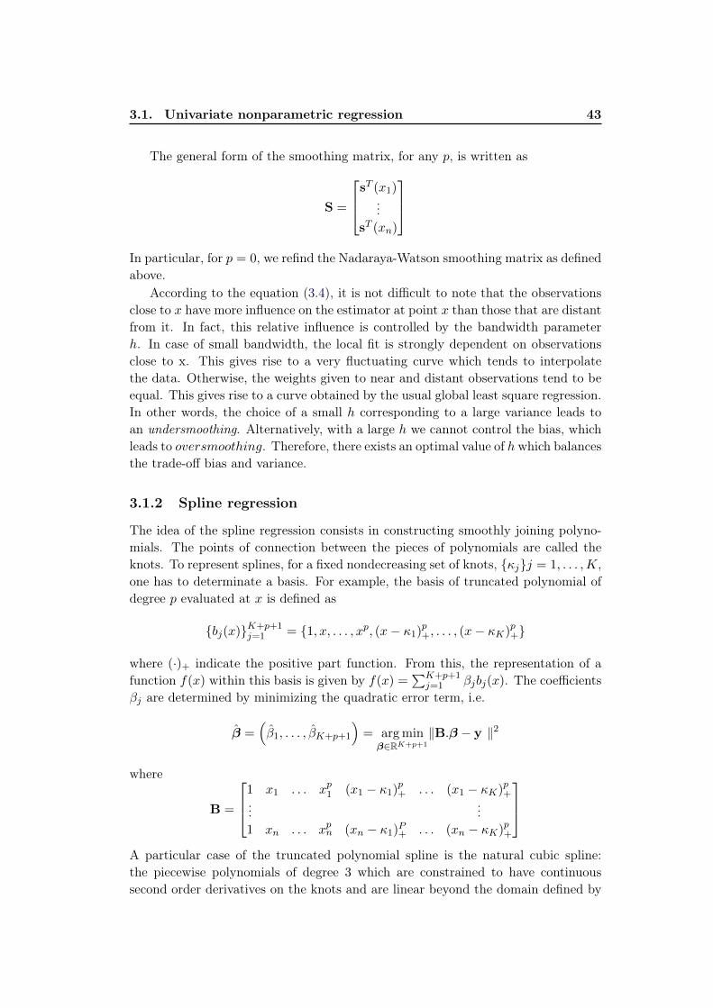
3.1. Univariate nonparametric regression 43
The general form of the smoothing matrix, for any p, is written as
S =
sT (x1)...
sT (xn)
In particular, for p = 0, we refind the Nadaraya-Watson smoothing matrix as definedabove.
According to the equation (3.4), it is not difficult to note that the observationsclose to x have more influence on the estimator at point x than those that are distantfrom it. In fact, this relative influence is controlled by the bandwidth parameterh. In case of small bandwidth, the local fit is strongly dependent on observationsclose to x. This gives rise to a very fluctuating curve which tends to interpolatethe data. Otherwise, the weights given to near and distant observations tend to beequal. This gives rise to a curve obtained by the usual global least square regression.In other words, the choice of a small h corresponding to a large variance leads toan undersmoothing. Alternatively, with a large h we cannot control the bias, whichleads to oversmoothing. Therefore, there exists an optimal value of h which balancesthe trade-off bias and variance.
3.1.2 Spline regression
The idea of the spline regression consists in constructing smoothly joining polyno-mials. The points of connection between the pieces of polynomials are called theknots. To represent splines, for a fixed nondecreasing set of knots, κjj = 1, . . . ,K,one has to determinate a basis. For example, the basis of truncated polynomial ofdegree p evaluated at x is defined as
bj(x)K+p+1j=1 = 1, x, . . . , xp, (x− κ1)p+, . . . , (x− κK)p+
where (·)+ indicate the positive part function. From this, the representation of afunction f(x) within this basis is given by f(x) =
∑K+p+1j=1 βjbj(x). The coefficients
βj are determined by minimizing the quadratic error term, i.e.
β =(β1, . . . , βK+p+1
)= arg minβ∈RK+p+1
‖B.β − y ‖2
where
B =
1 x1 . . . xp1 (x1 − κ1)p+ . . . (x1 − κK)p+...
...1 xn . . . xpn (xn − κ1)P+ . . . (xn − κK)p+
A particular case of the truncated polynomial spline is the natural cubic spline:the piecewise polynomials of degree 3 which are constrained to have continuoussecond order derivatives on the knots and are linear beyond the domain defined by

44Chapter 3. Application of Bayesian penalized spline regression for
internal modeling in life insurance
these knots. The natural condition of linearity on the edges implies the followingexpression of the natural basis of truncated polynomials for cubic splines
bj(x)Kj=1 = 1, x, d1(x)− dK(x), . . . , dK−2(x)− dK(x)
where dk(x) =(x−κk)3
+−(x−κK)3+
κk−κK [50]. The proof of this result is quite simple. Let usconsider the truncated power series representation for cubic splines with K knots
g(x) =3∑j=0
βjxj +
K∑k=1
θk(x− κk)3+ (3.6)
Using the natural boundary conditions for natural cubic splines leads to
β2 = β3 = 0,K∑k=1
θk =K∑k=1
κkθk = 0
or equivalently θK = −∑K−1
k=1 θk and θK−1 = −∑K−2
k=1(κk−κK)
(κK−1−κK)θk. Substitutingthese conditions into (3.6) implies our natural cubic splines basis.
The B-splines basis is however more suitable for calculations. This basis isobtained by linear combinations of the truncated polynomials. Namely, let ξ =
ξ0, . . . , ξN+1 be a sequence of non-decreasing real numbers such that
ξ0 ≤ · · · ≤ ξN+1
Define the augmented knot set
ξ−(m−1) = · · · = ξ0 ≤ · · · ≤ ξN+1 = · · · = ξN+m
where we have appended m − 1 times the lower and upper boundary knots ξ0 andξN+1. The B-splines basis is defined by
Bj,k(x) = (ξj+k − ξj)[ξj , . . . , ξj+k](· − x)k−1+
for all x ∈ R, j = −(m − 1), . . . , N + m − k and k = 1, . . . ,m. In the previousdefinition, we used the divided differences operator [t0, . . . , tn] which is defined byrecursion as follows
[t0]f = f(t0), [t0, . . . , tn]f =[t1, . . . , tn]f − [t0, . . . , tn−1]f
(tn − t0).
Since a B-spline is a linear combination of truncated power functions, so is con-tinuous from the right. Furthermore, we can recursively define a set of real-valuedfunctions Bj,k as follows:
Bj,1(x) = Iξj≤x<ξj+1
Bj,k(x) = ωj,k(x)Bj,k−1(x) + (1− ωj+1,k(x))Bj+1,k−1(x) for 1 < k ≤ m

3.2. Multivariate non-parametric regression 45
where ωj,k =x−ξj
ξj+k−ξj . For the above computation we define 0/0 as 0. These twodefinitions are equivalent. (see [18, 45]). Here are some of the properties: each B-spline has support in a finite interval; the B-splines form a partition of unity, i.e.∑N+m−k
j=−3 Bj,k(x) = 1; each B-spline Bj,k(x) is a piecewise polynomial of order k−1.These are local support functions, which implies that the corresponding matrices
are strip matrices. This base is constituted by K + 2 functions, the B-splines arenot natural splines, they have different restrictions on the edges.
3.2 Multivariate non-parametric regression
The multidimensional generalization of the problem (3.1) is as follows:
Y = f(X1, . . . , Xd) + ε (3.7)
with (X, Y ) = (X1, . . . , Xd, Y ) a random vector, ε a random variable independentof X such that E(ε) = 0, Var(ε) = σ2.
The adjustment of Y to a d-dimensional surface can be done by generalizing thekernel smoothing [47] as
KΛ(x,x′) =1
det(Λ)K(Λ−1(x− x′)
)(3.8)
where x = (x1, . . . , xd)T , x′ = (x′1, . . . , x
′d)T , and Λ is a positive definite, symmetric
matrix.Many possibilities exist for defining the kernel K(·). For example, it can be
defined as the d-product of uni-dimensional kernel, i.e. K(t) =∏dj=1K(tj), or by
a single uni-dimensional kernel, i.e. K(t) = K(‖t‖), where the choice of the normdetermines the shape of the neighborhoods. Another possibility is to generalizedirectly the uni-dimensional kernel functions.
The generalization of the Nadaraya-Watson (3.2) is thus
fNW (x) =
∑ni=1 yiKΛ(x,xi)∑ni=1KΛ(x,xi)
(3.9)
where xi = (xi1, . . . , xid)T .
The generalization of the minimization problem (3.3), in the particular case oflinear local regression, is
n∑i=1
(yi − β0 − (x− xi)T .β1
)2KΛ(x,xi) (3.10)
where β1 is a d× 1 dimensional vector.For cubic splines, one possibility is to generalize the penalization of the second
derivative to a plate-penalty [44], i.e.∫· · ·∫ d∑
j=1
(∂2f
∂x2j
)2
+∑j,k
(∂2f
∂xj∂xk
)2 d∏j=1
dxj . (3.11)

46Chapter 3. Application of Bayesian penalized spline regression for
internal modeling in life insurance
3.2.1 Some problems in high dimensional analysis
In the multidimensional case, non-parametric regression presents several problems.First, graphical representation is not possible for more than two explanatory vari-ables, and interpretation becomes difficult.
Second, the local methods approach fails in high dimension. This is the so-calledproblem of "curse of dimensionality" [12], which manifests itself in various ways. Forexample, assume that the observations of the explanatory variables are uniformlydistributed in a d-dimensional unit cube (d = 2, d = 10). To recover a percentageof the data p = 10%, the side length of a sub-cube should be p1/d. The length ofthe side is 0.32, for d = 2, and 0.79, for d = 10. For high d, these neighborhoodsare no longer local (the length of the side is very close to unity, so the sub-cube isvery close to the global cube). As a result, when the dimension increases, eitherlarger neighborhoods must be taken, implying global averages and therefore largebias, or the percentage of the data must be reduced which implies averaging over afew observations and therefore large variances of the adjustment [50].
Third, in high dimension setting, most data sets are usually "embedded" onsmaller dimensional manifolds. If these manifolds are hyper-planes, we encounterthe collinearity problem of the explanatory variables. If these manifolds are regular,we encounter a more general problem of concurvity [20,49].
3.2.2 Dimension Reduction Techniques
A solution to the high dimensional problems is to assume that the regression functionhas a certain structure. These non-parametric techniques remain flexible tools. Theprice to pay is the possible erroneous specification of the model.
The techniques based on dimension reduction principles are the additive models,which assume that the regression function is a sum of mono-variate functions in eachof the variables, projection pursuit models, close to multilayer perception neuralnetworks, and regression trees.
Projection pursuit
The algorithm of projection pursuit is to build an additive regression model of theform [38,65]:
Y =
K∑k=1
fk(αTk .X) + ε (3.12)
where ε is a random variable such that E(ε) = 0, Var(ε) = σ2 and independent ofthe explanatory variables.
The vector explanatory variables is projected on K directions αkk=1,...,K . Theregression surface is constructed by estimating one-dimensional regressions fk ap-plied to projections. The directions αkk=1,...,K and the number of terms K arechosen by model selection methods such as generalized cross validation.

3.2. Multivariate non-parametric regression 47
The advantage of this technique is that it allows easy processing of low densitydata. The model is also little constraint. Nevertheless, for K > 1, this modelpresents difficulties of interpretation: it is difficult to evaluate the contributions ofeach variable. For K = 1, the model is known as single−index model.
Projection pursuit techniques are often compared to multilayer perception neuralnetworks. These two methods extract linear combinations of inputs, and then modelthe output variable as a nonlinear function of these input variables. However, thefunctions fk of the projection pursuit are different and non-parametric, whereas theneural networks use a simpler activation function, normally the softmax (or logistic)function. In the case of projection pursuit, the number of "layers" is set at two 1
and the number of functions K is also predefined, which is not the case for neuralnetworks.
Regression trees
Regression trees divide the space of the explanatory variables into a set of hyper-cubes. A simple model (for example, a constant) is then fitted to each hyper-cubeas
f(x) =K∑k=1
αkIx∈Rk (3.13)
withK the number of partitions of the space of the explanatory variables, Rk disjointregions, αk the constant that models the response in the region. The algorithmsimultaneously decides the partition and the values of the parameters αkk=1,...,K .
Regression trees have the advantage of conceptual simplicity and the ability tointerpret. Their limitations are instability and lack of continuity of the regressionsurface.
3.2.3 Additive models
Additive models assume that the regression function can be written as a sum offunctions of the explanatory variables [48,107]:
Y = α0 +
d∑j=1
fj(Xj) + ε (3.14)
where ε is independent of X = (X1, . . . , Xd), E(ε) = 0 and Var(ε) = σ2; α0 is aconstant, fj , j = 1, . . . , d are the univariate functions such that EXj [fj(X)] = 0.This condition of identifiability implies that EX[Y ] = α0 [49].
Additive models can be introduced as a generalization of the linear regressionmodels. This is the basic tool for modeling the relationship between the continuousresponse variable and the explanatory variables:
Y = α0 + α1X1 + · · ·+ αdXd + ε (3.15)1More precisely, we have X −→ αTk .X −→ fk(αTk .X) −→ Y.

48Chapter 3. Application of Bayesian penalized spline regression for
internal modeling in life insurance
where ε is independent of X, E(ε) = 0 and Var(ε) = σ2.The assumption of linear dependence of EX[Y ] in each of the explanatory vari-
ables is a strong assumption. When this assumption is not verified, one way toextend the linear model is the additive model. The non-parametric form of fj givesmore flexibility to the model, while the additive structure preserves the possibil-ity of representing the effect of each variable. The model can be represented byone-dimensional functions describing the roles of explanatory variables in responsemodeling, which facilitates interpretation. However, the simplicity of the linearmodel is lost. A new problem appears: the selection of smoothing parameters, rep-resenting the complexity of each component of the model. Here we will list someproperties of the additive models.
Interpretability: The joint effect of the explanatory variables on the responsevariable is expressed as a sum of the individual effects. These individual effects showhow the expectation of the response varies when one of the components varies whilethe others are fixed to any values. Thus, the individual functions can be representedseparately in order to visualize the effect of each explanatory variable, making theresult intelligible. The possibility of representing the effects of the variables directlyat the same time gives indications on the importance of each of the variables.
Scourge of dimensionality: By restricting the nature of the dependencies,the problems related to the high dimension are mitigated: the response is modeledas the sum of uni-dimensional functions of the explanatory variables, instead of be-ing modeled by multidimensional functions. Therefore, the number of observationsrequired increases linearly with d (and not exponentially).
Consider the estimation of the regression function (3.7). The optimal asymptoticrate for the estimate of f is n−[m/(2m+d)], where m is an index of the regularity ofthe function f is m − 1 times continuously differentiable and its m-th directionalderivatives exist) [106]. On the other hand, if f is additive, the optimal rate reachesthe uni-dimensional convergence rate n−[m/(2m+1)] [108]. In this sense, the additivemodels are considered as dimension reduction techniques.
Invalid model: The model is poorly specified when the explanatory variablesinteract. That is, the effect of the variations of an explanatory variable on theresponse depends on the values adopted by the other explanatory variables.
Suppose the general multiple regression model (3.7), where the function f(·) isa smooth function. Assuming that the observations xij are contained in a regionwhere the curvature of the function f is small, then the additivity (and linearity) canbe justified by a first-order Taylor expansion f(x) ≈ f(x′) +Df(x′)(x− x′), wherex′ is within the region defined by the observations and Df indicates the gradient off . If the curvature of f is high, the Taylor expansion requires, at least, quadraticterms and cross terms in two variables. When only the former are needed, the modelis always additive, although it incorporates "nonlinear" terms.
Adaptability: The interest of additive models is their ability to model therelationship between variables in an intuitive way, but also the possibility of adaptingthe model to simpler or more complex situations. When components do not requirenonparametric modeling, they can be reduced to linear components. Also, when

3.3. Notations and requirements for the fitting process 49
interactions exist between certain variables, quadratic (or higher order) terms canbe integrated into the model.
Part II-Application of Bayesian penalized spline regres-sion for internal modeling
3.3 Notations and requirements for the fitting process
3.3.1 Risk factors
As will be seen later, we use the term "risk factors" to refer to the underlyingparameters that may impact the balance sheet. As discussed in Chapter 2 and inAppendix B, we might notice that there are several risk factors, which may affectan insurance firm’s economic balance sheet. These risks can generally be classifiedinto the following categories:
1. asset-related risks (interest rates, equity and property prices, credit spreads):asset-liability impacts of variances in underlying parameters across all lines ofbusiness;
2. insurance risks: claims (mortality/morbidity/longevity), discontinuances, ex-penses, including effects of both actual experience over the period of assess-ment as well as the impact of that experience on the closing liability assess-ment;
3. counterparty risks: risk of default by key counterparties such as reinsurers;
4. operational risks.
There are some risks which could affect the company but have little impact on theasset position (reputation risk is an example). There are some risks which not bemitigated by holding capital against them (liquidity risk is an example). Theserisks should be considered in the broader risk management framework but mightnot feature in the calculation of Economic Capital.
The approach to quantifying risks will vary by risk type. This includes:
• factor-based methods, where a factor is applied to a driver to approximate theimpact of a risk;
• stress testing, where a specific shock is defined and the impact of that shockon the balance sheet is determined;
• stochastic modelling, where a full distribution of shocks are modelled, produc-ing a full distribution of own funds outcomes.
Like many other proxy models (e.g. Curve Fitting, LSMC), only stochastic riskfactors are taken into account in this methodology.

50Chapter 3. Application of Bayesian penalized spline regression for
internal modeling in life insurance
3.3.2 Loss function
The loss function in life insurance is a function defined as the change in Basic OwnFunds due to the realization of different economic states of the world. Mathemat-ically, let us denote by (RF1, . . . , RFd) a d-tuple standing for the underlying riskfactors and by (x1, . . . , xd) another d-tuple representing the shock applied at thecurrent state. The loss function is then defined as:
φ(x1, . . . , xd) = BOFt=0 (RF1, . . . , RFd)−BOFt=0+ (RF1(1 + x1), . . . , RFd(1 + xd))
(3.16)In the Solvency II environment, the value of each balance sheet part corresponds tothe expected value of the discounted future cash-flows under a risk-neutral proba-bility Q. Let
• DF(0, t) be the stochastic discount factor in terms of a risk free instantaneousinterest rate rs, i.e. DF(0, t) = e
∫ t0 rsds;
• Rt be the company's profit in period t.
Under this notation, the Basic Own Funds at the initial date is calculated in thefollowing manner:
BOFt=0(RF1, . . . , RFd) = EQ
[T∑u=1
DF(0, u)Ru | (RF1, . . . , RFd)
]From this we may rewrite the loss function (3.16) in terms of the conditional expectedvalue with respect to capital loss.
Namely, let
Y = BOFt=0(RF1, . . . , RFd)−T∑u=1
DF(0, u)Ru |(RF1(1+x1),...,RFd(1+xd))
be the potential capital loss which is a random variable whose conditional distri-bution depends on the x1, . . . , xd. The loss function (3.16) can be equivalentlyrewritten as:
φ(x1, . . . , xd) = EQ (Y | x1, . . . , xd) (3.17)
For latter use, let us define the standalone loss functions φj(xj) which is of theform:
φj(xj) = EQ (Y | 0, . . . , xj , . . . , 0) (3.18)
and the excess loss function which is expressed as:
φ1d(x1, . . . , xd) = EQ (η | x1, . . . , xd) (3.19)
with η = Y −∑d
j=1 φj(xj) the residual loss of capital. From this, it is easily seenthat the following relation holds:
φ(x1, . . . , xd) =d∑j=1
φj(xj) + φ1d (x1, . . . , xd) . (3.20)

3.3. Notations and requirements for the fitting process 51
Figure 3.1: Here we illustrate the empirical SCR estimation with N1 outer simula-tions.
Stand-alone loss functions are useful for risk monitoring, as they are used to analyzethe contribution of each risk factor to the capital requirements. In fact, to havestand-alone loss functions allows to classify and quantify risk exposure to risk factors,which corresponds to a useful tool for steering the activity. Thus, this specificdecomposition for stand-alone loss functions is fully aligned with market practice.As a result, the standalone loss functions should be independently calibrated so asnot to modify the other estimators.
3.3.3 Approximation of a shock at t = 0+
As seen previously, the Nested Simulation approach requires the realization of thereal world scenarios between t = 0 and t = 1. In practice, one usually relies on adifferent approach, which consists of performing the approximation of a shock att = 0+. Regarding the market risks, this means that the market value of financialinstruments are modified right after their initialization. This approximation is inline with the standard formula approach, where the defined shocks are to be appliedinstantaneously on the balance sheet. In the standard model, the SCR is evaluatedvia the "square-root" formula based on a modular approach. In our setting (internalmodel), the SCR is defined as the 99.5%-quantile of the loss function (see Section3.3.2 for the definition of the loss function), i.e.
SCR = q99.5%(φ) (3.21)
As will be seen later, further analyses will be performed to highlight the reliabilityof our assumption (3.21) and the resulting estimate. Namely, we carry out thecomparison between the SCR estimated by Nested Simulations approach and theSCR estimated by our method.

52Chapter 3. Application of Bayesian penalized spline regression for
internal modeling in life insurance
3.4 Methodology description
We assume that the functional components φ1, . . . , φd, φ1d are regular enoughand every standalone loss function can be thus approximated by polynomial splinefunction (see Appendix D.7). To guarantee the granularity, we will estimate in-dependently each standalone loss functions by applying the Bayesian penalizedspline regression (see Appendix D.3). Regarding the Excess Loss function, evenif φ1d(x1, . . . , xd) is not genuinely additive, an additive approximation to φ1d maybe sufficiently accurate as well as being readily interpretable. We define φ∗1d beingof the form:
φ∗1d (x1, . . . , xd) = h0 +
d∑j=1
hj (xj) +∑
1≤j<j′≤dhjj′
(xj × xj′
)(3.22)
To ensure identifiability of each of the functional components, we include theintercept h0 and the functions hj , hjj′ are chosen subject to the constraints1n
∑nν=1 hj(x
(ν)j ) = 1
n
∑nν=1 hjj′(x
(ν)j × x
(ν)j′ ) = 0 where
(x
(ν)1 , . . . , x
(ν)d
)ν=1,...,n
are
the design points as will be seen later. Then φ∗1d is the best additive approximationto φ1d in the sense of mean squared error. In the case that φ1d is additive, we thenhave φ1d = φ∗1d. The Excess Loss function will be thus estimated via the additivemodel (3.22). With a slight abuse of notation, we use the same symbol here as inEquation (3.20), i.e.:
φ(x1, . . . , xd) =d∑j=1
φj(xj) + φ∗1d (x1, . . . , xd) .
Confidence intervals are of primary importance in many practical applications ofhow accurate the estimate can predict. As remarked by Nychka [84], “one limitationin applying spline methods in practice, however, is the difficulty in constructingconfidence intervals or specifying other measures of the estimate’s accuracy”. Wahba[115] suggested a Bayesian approach to derive the point-wise asymptotic confidenceinterval. Surprisingly, these Bayesian asymptotic confidence intervals work welleven when evaluated from the frequentist viewpoint. As it stands, we will usethis approach to derive the asymptotic confidence intervals for the standalone lossfunctions estimation as well as the excess loss function estimation. However, wewould like to point out that the confidence bands do not incorporate approximationerrors from the choice of the regression function. This remark will be shown in thederivation which can be found in Appendix D.4 and Appendix D.5.
The proposed methodology is summarized in five steps:
• Fitting points selection: The first step consists of generating the design pointsx(ν)
j ν=1,...,njj=1,...,d . Since the sample size is limited by calculation time, only signif-
icant and comparable point are mainly considered. In fact, we are ultimatelyinterested in calculating a percentile on the economic own funds distribution,

3.4. Methodology description 53
it is consequently important to know with accuracy what will be the potentialloss with a security level of 99.5% rather than having a perfect estimation ofthe loss function for every realistic scenario even though the final objective isto get the most accurate possible fitting. Therefore, a sufficient number of “tailscenarios” is required in order to estimate properly the economic own fundstail distribution. To this end, we assume that the desired tail scenarios lie inthe tail of distribution of each underlying risk factor and this latter one definesthe 99.5th-percentile region. The determination of the 99.5th-percentile regiondepends however upon the risk-factor considered. For example, we know thatthe falling equity markets implies the negative impact on BOF, and thus in-creases the loss capital. Therefore, the 99.5th-percentile for the Equity riskis placed on the left tail of its distribution which is defined as the intervalbetween the 0.01th percentile and the 10th-percentile. Concerning the convex(or U-shaped) loss functions, such as the Interest rate loss function, the tailscenarios should be picked from both extremes of its distribution since it is notclear ex ante of whether the highest or lowest values of interest rates would bemost problematic. All design points located outside of the 99.5th-percentileregion can be selected randomly and uniformly.
• Standalone loss functions estimation: Using the ALM model described in Sec-tion 3.5.1.4, one values the empirical estimate of the standalone losses for eachselected design points x(ν)
j ν=1,...,njj=1,...,d , that is φj(x
(ν)j ) = 1
N2
∑N2k=1 Y
(k)
|x(ν)j
with
N2 the number of inner scenarios and Y(k) the loss of capital associated to thek-th inner scenario given the market stress condition x(ν)
j . Next one appliesthe Bayesian penalized spline regression model to smooth the data by solvingthe following optimization problem:
minβ∈Rpj+Kj+1
[ nj∑ν=1
(φj
(x
(ν)j
)−B
(x
(ν)j
)βj
)2+ λjβ
Tj Djβj
], ∀j = 1, . . . , d
(3.23)where B(x) =
(1, x, x2, . . . , xpj , (x− κ1)
pj+ , . . . , (x− κKj )
pj+
)T ∈ R1+pj+Kj isthe truncated pj-polynomial basis with Kj knots κ1, . . . , κKj, the symbol(·)+ stands for the Heaviside step function and Dj is the block diagonal ma-trix diag
(01+pj ,1Kj
). (For the detailed description of the Bayesian penalized
spline regression, please refer to Appendix D). Let Bj be the nj×(1+pj+Kj)
matrix whose i’s row equals B(x
(i)j
)Tand Φj =
(φj
(x
(1)j
), . . . , φj
(x
(nj)j
))T,
the estimate of βj is then given by:
βj =(BTj Bj + λjDj
)−1BTj Φj (3.24)
for j = 1, . . . , d. From this it follows that Φj =(φj
(x
(1)j
), . . . , φj
(x
(nj)j
))=
Bj βj .

54Chapter 3. Application of Bayesian penalized spline regression for
internal modeling in life insurance
The deviation of φj(x
(ν)j
)from φ
(x
(ν)j
)is characterized by the 1−α Bayesian
asymptotic confidence interval having the form:
P(|φj(x
(ν)j
)− φ
(x
(ν)j
)| ≤ ∆
(ν)j,α
)→ 1− α (3.25)
where ∆(ν)j,α = max
(∣∣∣∣∣zα/2√(
E(Mj)− E(Bj)2)[
VΦj
]νν± E (Bj)
√[VΦj
]νν
∣∣∣∣∣),
zα/2 is the critical point from a standard normal distribution and the explicit
form of E(Mj), E(Bj) and VΦjare given in Appendix D.4.
• Excess loss function estimation: Again we use the ALM model and the stan-dalone loss functions estimators to value the empirical excess losses at eachdesign points x(ν)
1d =(x
(ν)1 , . . . , x
(ν)d
)for ν = 1, . . . , n, that is
φ1d (xν1d) =1
N2
N2∑k′=1
Y(k′)
|x(ν)1d
−d∑j=1
φj
(x
(ν)j
)wherein Y(k′)
|x(ν)1d
is the capital loss associated to the k′-th inner scenario given
the market stress condition x(ν)1d . These are considered to be the responses
variables. To ensure that independence is not broken, scenarios used to derivethe excess loss function should be different from those used in the standaloneloss functions calibration. The algorithm to derive the functional componentshj , hjj′ estimators of excess loss function is analogue to that of the standaloneloss function. The computation is tedious and can be found in Appendix D.5,so we will omit it here. For later use, we define the 1−α Bayesian asymptoticconfidence interval for hj , hjj′
∆(ν)J,α = max
(∣∣∣∣∣zα/2√(
E (MJ)− E (BJ)2)[
VhJ
]νν± E (BJ)
√[VhJ
]νν
∣∣∣∣∣)
(3.26)where J can be j or jj′, zα/2 is the critical point from a standard normal
distribution and the explicit form of E(MJ), E(BJ) and VhJare given in
Appendix D.5.
• Loss function estimation error control: We will now investigate the control ofthe deviation of φ from φ at an arbitrary design points x(ν) = (x
(ν)1 , . . . , x
(ν)d ).
Obviously, we have|φ(x(ν))− φ(x(ν))| >d∑j=1
∆(ν)j,α +
∑J
∆(ν)J,α
⊂ d⋃j=1
|φj(x
(ν)j
)− φj
(x
(ν)j
)| > ∆
(ν)j,α
∪(⋃J
|hJ(x
(ν)J
)− hj
(x
(ν)J
)| > ∆
(ν)J,α
)(3.27)

3.4. Methodology description 55
where we used the notation x(ν)jj′ = x
(ν)j × x
(ν)j′ . From this it follows that the
probability of deviation of φ(x(ν)) from φ(x(ν)) is asymptotically bounded by
P
|φ(x(ν))− φ(x(ν))| >d∑j=1
∆(ν)j,α +
∑J
∆(ν)J,α
≤ 1− (1− α)d(d+3)
2 (3.28)
The derivation of this result can be found in Appendix D.6.
Motivated by this, we can estimate SCR by SCR = q99.5
(φ)
its empirical
99.5th-percentile derived from φ. In this stage, φ ≡ φ(X) is a random variable withX = (X1, . . . , Xd) the realistic random market state or the primary simulation statewhose marginal distribution is PX . Let fφ denote the density function of φ(X).
To control the probability of deviation of the target SCR from its estimate, wewill need certain conditions to make the theory work. First of all, it is important toclarify that as will be seen below, the resulting confidence band will not incorporatethe approximation error from the choice of the regression function.
Let us introduce some notation, definitions that will be used in the sequel. Wedefine the (L,Ω)-Lipschitz class of functions, denoted Σ(L,Ω), as the set of functiong : Ω→ R satisfy, for any x, x′ ∈ Rd, the inequality:
|g(x′)− g(x)| ≤ L‖x′ − x‖
with Ω ⊂ Rd and ‖x‖ , (x21 + · · · + x2
d)1/2. Let r > 0. We define B(a, r) =
x ∈ Rd | ‖a − x‖ ≤ r. We denote by Vφ = x ∈ Rd | φ(x) = q99.5%(φ) andVφ = x ∈ Rd | φ(x) = q99.5%(φ) the closed set of the 99.5th-percentile scenariosfor φ and φ respectively.
Let Γ denote the available sampling budget used to calibrate φ. Based on thework of Aerts et al. [2], it is straightforward to deduce that for λφj (Γ) and λhJ (Γ)
tending to 0, the estimate φ converges in mean square to φ as Γ→∞. Furthermore,by Markov’s inequality, convergence in mean square of φ leads to the convergencein probability of φ(x) to φ(x) for every x ∈ Rd. This implies that for every x∗ ∈ Vφ,there exists a random sequence x∗(Γ) ∈ Vφ converges in probability to x∗.
Introduce now three assumptions on φ, φ and x∗(Γ) that will be used in the laststep:
ASSUMPTION 1: Suppose that φ ∈ Σ(L,Ω) where L > 0 and Ω(⊃ Vφ) is anopen subset of Rd.
ASSUMPTION 2: For any x∗ ∈ Vφ and r > 0, there exists two positive constantsξ(r, d), γ(r, d) such that
P(‖x∗ − x∗(Γ)‖ > r
)≤ ξ(r, d)Γ−γ(r,d)
for large enough Γ.ASSUMPTION 3: For any choice of x∗ ∈ Vφ and α ∈ (0, 1), there exists two
positive constants r(Γ) and ∆(α,Γ), with r(Γ)Γ→∞−−−→ 0, such that
P(| φ(x)− φ(x) |> ∆(α,Γ)
)≤ 1− (1− α)
d(d+3)2 , ∀x ∈ B(x∗, r(Γ))
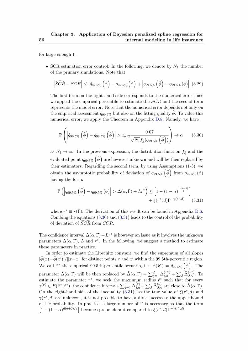
56Chapter 3. Application of Bayesian penalized spline regression for
internal modeling in life insurance
for large enough Γ.
• SCR estimation error control: In the following, we denote by N1 the numberof the primary simulations. Note that∣∣∣SCR− SCR∣∣∣ ≤ ∣∣∣q99.5%
(φ)− q99.5%
(φ)∣∣∣+∣∣∣q99.5%
(φ)− q99.5% (φ)
∣∣∣ (3.29)
The first term on the right-hand side corresponds to the numerical error sincewe appeal the empirical percentile to estimate the SCR and the second termrepresents the model error. Note that the numerical error depends not only onthe empirical assessment q99.5% but also on the fitting quality φ. To value thisnumerical error, we apply the Theorem in Appendix D.8. Namely, we have
P
∣∣∣q99.5%
(φ)− q99.5%
(φ)∣∣∣ > zα/2
0.07√N1fφ(q99.5%
(φ)
)
→ α (3.30)
as N1 →∞. In the previous expression, the distribution function fφ and the
evaluated point q99.5%
(φ)are however unknown and will be then replaced by
their estimators. Regarding the second term, by using Assumptions (1-3), weobtain the asymptotic probability of deviation of q99.5%
(φ)
from q99.5% (φ)
having the form:
P(∣∣∣q99.5%
(φ)− q99.5% (φ)
∣∣∣ > ∆(α,Γ) + Lr∗)≤[1− (1− α)
d(d+3)2
]+ ξ(r∗, d)Γ−γ(r∗,d) (3.31)
where r∗ ≡ r(Γ). The derivation of this result can be found in Appendix D.6.Combing the equations (3.30) and (3.31) leads to the control of the probabilityof deviation of SCR from SCR.
The confidence interval ∆(α,Γ)+Lr∗ is however an issue as it involves the unknownparameters ∆(α,Γ), L and r∗. In the following, we suggest a method to estimatethese parameters in practice.
In order to estimate the Lipschitz constant, we find the supremum of all slopes|φ(x)−φ(x′)|/‖x−x‖ for distinct points x and x′ within the 99.5th-percentile region.We call x∗ the empirical 99.5th-percentile scenario, i.e. φ(x∗) = q99.5%
(φ). The
parameter ∆(α,Γ) will be then replaced by ∆(α,Γ) =∑d
j=1 ∆(x∗)j,α +
∑J ∆
(x∗)J,α . To
estimate the parameter r∗, we seek the maximum radius r∗ such that for everyx(ν) ∈ B(x∗, r∗), the confidence intervals
∑dj=1 ∆
(ν)j,α+
∑J ∆
(ν)J,α are close to ∆(α,Γ).
On the right-hand side of the inequality (3.31), as the true value of ξ(r∗, d) andγ(r∗, d) are unknown, it is not possible to have a direct access to the upper boundof the probability. In practice, a large number of Γ is necessary so that the term[1− (1− α)d(d+3)/2
]becomes preponderant compared to ξ(r∗, d)Γ−γ(r∗,d).

3.5. Numerical study 57
Figure 3.2: Initial Balance Sheet used to value the prudential balance sheet.
3.5 Numerical study
Being aware of the limitations of the ALM model considered in this paper, the areaof use of this cash-flow generator depending on only a few risk factors is sufficientin the context of this study. That is to say, the study serves as illustration for ourproposed methodology. In practice, note that for many life insurance companies,the number of risk factors is often very large, e.g., over 100. Therefore, the efficiencyas well as the performance of this approach compared with the existing approachesremain unknown for practical problems and can be the subject of future research.
3.5.1 ALM modeling
In this section, we recall in a concise way the main lines of the operation of an actu-arial cash flow simulator that is used today by life insurers to value their prudentialbalance sheet. All the details of our ESG and ALM cash-flow simulator are givenin Chapters A and B.
3.5.1.1 Initial balance sheet
We model the prudential balance sheet of an insurance company that sells exclu-sive savings contracts in euros. The initial balance sheet of the modeled insurancecompany is defined as follows:
Assets backing mathematical reserves consist of cash, equities/real estate andbonds, by convention, up to 5%, 15% and 80%, respectively. Assets backing liquidityrisk provision (PRE ), profit-sharing provision (PPE ), capitalization reserve and ownfunds are not explicitly modeled and implicitly considered to be 100% of cash (seeFigure 3.2).
The cash-flow simulator considers the risk neutral evolution of financial risk fac-tors on the balance sheet and these trajectories run for 50 years. At each time step,the cash flows of assets and liabilities are calculated and the company’s manage-

58Chapter 3. Application of Bayesian penalized spline regression for
internal modeling in life insurance
ment strategy is implemented (calculation of the profit-sharing rate, allocation ofprovisions, distribution of dividends to shareholders, etc.).
3.5.1.2 Liabilities
Regarding the liabilities, the contracts in the liabilities are exclusively savings con-tracts in euros with minimum guaranteed rates (MGR) and redemption rights. Inaccordance with the Solvency II Directive, the valuation of the prudential balancesheet is carried out in run-off on insurance liabilities, which means that no newfuture production is considered and under the assumption of continuity of activitieson the assets side (maintenance of target allocation, management decisions, etc.).
Savings contracts generally allow policyholders to withdraw partially or totallytheir savings. We can distinguish two types of redemptions in life insurance:
1. Conjunctural surrenders: these are the redemptions linked to the economicsituation and the performance of the insurer. They are usually estimatedfrom the difference between the rate served by the insurer and the rate servedby the competition.
2. Structural surrenders: these are the redemptions related to the characteristicsof the contract. For example, there is usually a wave of structural surrenderafter the 8 year seniority. This phenomenon is explained by the taxation oflife insurance, which becomes more favorable when it comes to redemptions ifthe contract has 8 year seniority.
The insurer makes its asset allocation according to the characteristics of itsliabilities (duration, MGR ...). If actual redemptions are greater than expectedredemptions, for the sake of liquidity, the insurer will be forced to sell assets thathave not matured, which may be a disadvantage if these assets are unrealized losses.Similarly, the insurer has to pay a capital or an annuity in case of death of the insuredto the beneficiary designated by the contract. Therefore, the risk of a buyout andmortality risk are two major risks for life insurers that results from a behavioralchange of insured persons. The modeling of these behaviors is therefore a crucialissue for the asset-liability management of an insurance company.
Insured mortality is assumed to be deterministic and the death rate is givenby the death table "TH0002" for men and "TF0002" for women 2. With respectto modeling the redemptions in our setting, the total redemption rate (TR) of themodel is calculated as the sum of the conjunctural surrender rate (CR), which is afunction of the spread between the rate expected by the insured and the last profitsharing rate served by the insured, and the structural surrender rate (SR), whichis determined on the policyholder’s seniority according to a historically calibratedredemption table.
2The TH-TF 0002 mortality table is built from the INSEE 2000 − 2002 table - re-spectively for the male population and for the female population. These are the regula-tory tables for life insurance contracts (other than life annuities) The table is available athttp://www.spac-actuaires.fr/jdd/public/documents/xls/TH-TF%2000-02.xls.

3.5. Numerical study 59
3.5.1.3 Assets
The asset portfolio of the insurance company consists of the following asset classes:cash, shares/real estate and bonds. Cash is remunerated at the risk-free rate. Wechoose the Hull & White one factor model to model the dynamics of short-terminterest rates. Namely, under the risk neutral probability Q, the instantaneousshort-term interest rate rt is governed by the following dynamics:
drt = (θt − art)dt+ σdWt
where σ represents the instantaneous volatility of the short rate, a is the mean-reverting speed and Wt the Brownian motion under the risk neutral probabilityQ. The time dependent parameter θt is determined by σ, a and the initial yieldcurve R(0, T ). As there is only one driving Brownian motion, all forward ratesare determined by the short rate. Since the dynamics of short rates depend on themean-reverting speed, the interest rate volatility and the initial yield curve, theselatter ones will thus completely determine the shape of the forward yield curves.In this study, we fix a = 0.35, σ = 0.5% and take the risk-free interest rate termstructures published by EIOPA as only input of the Hull & White model. Readerscan refer to [36] for more details of this model.
Shares/real estate are modeled by a geometric Brownian movement with con-stant dividend rate and log-normal volatility at 17.4%. The dividend or rent rate isadjustable. Here, the dividend rate is set at 3%, the rental rate at 5%. The treasurybond portfolio consists of government bonds whose probability of default is assumedto be zero.
3.5.1.4 ALM Model
The ALM simulator projects the assets and liabilities of the insurer over time. Thismakes it possible to determine at each time step the balance sheet and the value ofthe flows distributed to the policyholders on the one hand and to the shareholderson the other hand.
At each time step, along with the risk neutral trajectory, the ALM simulatorproceeds in 6 steps to forecasting the assets and liabilities by one year, calculatingthe cash flows of liabilities and assets, updating the balance sheet and determiningthe value of the outgoing flows:
1. Sale or purchase of assets to recover the target allocation at book value: 80%
bonds, 15% equities and 5% monetary.
2. Disseminate the stock market values over one year; calculate the dividend andthe bonds coupon received in respect of the year; construct the yield curve overone year; actualize the bonds market values; calculate the carrying amortizingamount of bonds over one year.
3. Determine death benefits and new premiums received during the past yearfor each point model. The death rates correspond to those of the TF0002

60Chapter 3. Application of Bayesian penalized spline regression for
internal modeling in life insurance
and TH0002 mortality tables. Benefits are assumed to be paid in the middleof the year. They are revalued at the rate used for the past year for halfa year. Moreover, the structural and conjunctural surrenders are evaluatedduring the year. Conjunctural surrender rates are valued as a function of thespread between the rate used in the previous year and the 10-year rate.
4. Periodic premiums received are invested in assets. Then, assets are eventu-ally sold to pay for benefits. After that, we recalculate the unrealized lossesassociated with non-bond assets on which the PRE is acquired or taken over.
5. The minimum and maximum available resources are calculated. They can bereached by playing on the achievement of the unrealized profits and losses,and of the resumption of PPE. The expected wealth is determined accordingto the performance of the financial markets. Finally, one determines the rateused for each point model, considering the different MGRs.
6. The distinct items of the closing balance sheet for year N are calculated byrevalorizing the Mathematical Provisions at the rate used as determined inthe previous step and the various balance sheet items (basic own funds, capi-talization reserve, PPE, PRE).
At the end of the trajectory, that is over 50 years, the assets are settled, the bal-ance sheet is updated and the balances of mathematical provisions and PPE aredistributed to policyholders.
3.5.2 Analysis of the loss functions
In this section, we present the results carried out to demonstrate the performance ofthe standalone as well as the excess loss functions fitting. As can be seen in Section(3.5.1), interest rate risk exists for all assets and liabilities for which the net assetvalue is sensitive to changes in the term structure of interest rates or interest ratevolatility. In the standard formula, the calculations of capital requirements in theinterest rate risk module are based on specified scenarios which are defined by adownward and upward stress of the term structure of interest rates. Inspired bythis idea, we restrict ourselves solely to consider the risk related to the level of theinitial yield curve.
To build stress scenarios, we apply a principal component analysis (explaining98% of the variability of the annual percentage interest rate change in each of thematurities in the underlying datasets) of historical term structure data from theyears 2007− 2017. As a result, the yield curve can be approximated as
R(0, T ) ≈ αPC1(0, T ) + βPC2(0, T ) + γPC3(0, T )
where PC1, PC2, PC3 are the first three forward curve loadings or principal com-ponent vectors (see Section 3.4.3 in [36] for more details). The PC1 represents thesituation that all forward rates in the yield curve move in the same direction. This
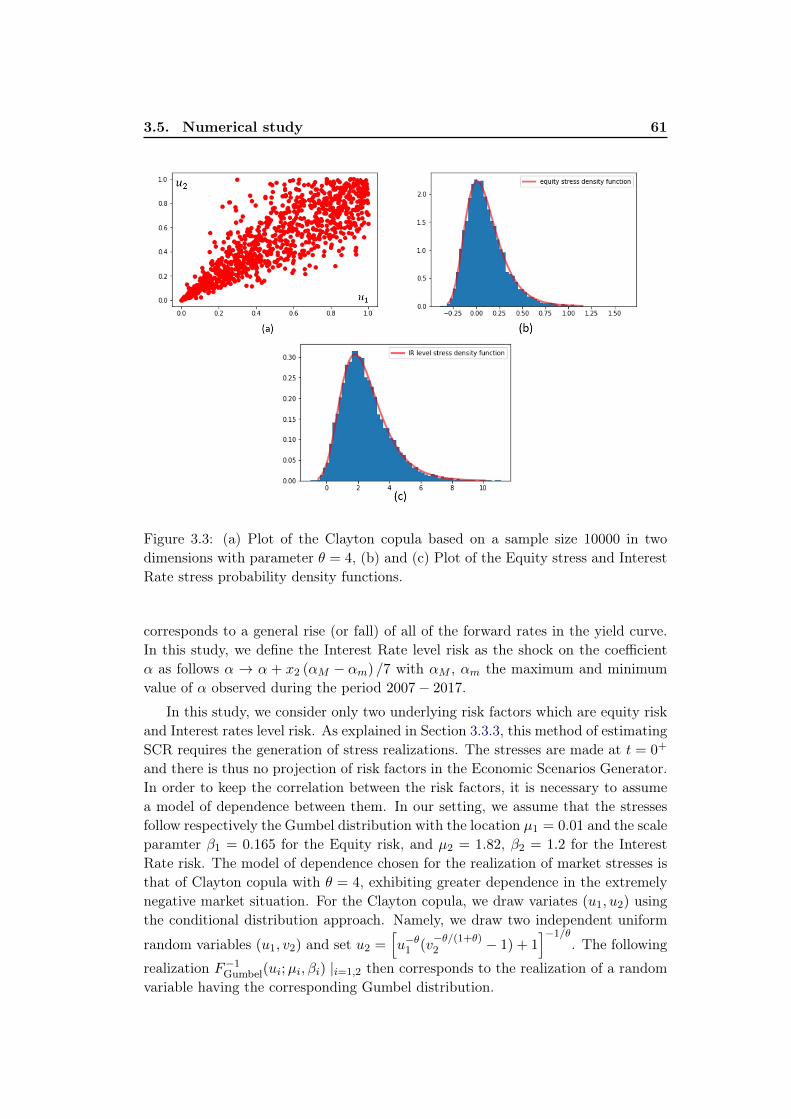
3.5. Numerical study 61
Figure 3.3: (a) Plot of the Clayton copula based on a sample size 10000 in twodimensions with parameter θ = 4, (b) and (c) Plot of the Equity stress and InterestRate stress probability density functions.
corresponds to a general rise (or fall) of all of the forward rates in the yield curve.In this study, we define the Interest Rate level risk as the shock on the coefficientα as follows α → α + x2 (αM − αm) /7 with αM , αm the maximum and minimumvalue of α observed during the period 2007− 2017.
In this study, we consider only two underlying risk factors which are equity riskand Interest rates level risk. As explained in Section 3.3.3, this method of estimatingSCR requires the generation of stress realizations. The stresses are made at t = 0+
and there is thus no projection of risk factors in the Economic Scenarios Generator.In order to keep the correlation between the risk factors, it is necessary to assumea model of dependence between them. In our setting, we assume that the stressesfollow respectively the Gumbel distribution with the location µ1 = 0.01 and the scaleparamter β1 = 0.165 for the Equity risk, and µ2 = 1.82, β2 = 1.2 for the InterestRate risk. The model of dependence chosen for the realization of market stresses isthat of Clayton copula with θ = 4, exhibiting greater dependence in the extremelynegative market situation. For the Clayton copula, we draw variates (u1, u2) usingthe conditional distribution approach. Namely, we draw two independent uniform
random variables (u1, v2) and set u2 =[u−θ1 (v
−θ/(1+θ)2 − 1) + 1
]−1/θ. The following
realization F−1Gumbel(ui;µi, βi) |i=1,2 then corresponds to the realization of a random
variable having the corresponding Gumbel distribution.

62Chapter 3. Application of Bayesian penalized spline regression for
internal modeling in life insurance
3.5.2.1 Standalone loss function fitting
For each variable considered, we take 25 points within the 99.5th-percentile regionand 25 points elsewhere. One possibility of selecting design points within the 99.5th-percentile region is to choose only comparable points. For example, one usuallychooses predefined percentiles such as the 0.5th-percentile and/or the 2th-percentile.The 0.5th-percentile is of a specific interest since it gives the required capital underthe assumption there is only one risk. In this paper, our choice of fitting points relieson following approach: the fitting points inside and outside of the 99.5th-percentileregion are selected randomly and uniformly. Each response variables Y is empiricallyevaluated byN2 = 40 inner scenarios. The most simple and straightforward "equallyspaced" knot placement method is used inside and outside of the 99.5th-percentilezone. For the natural cubic spline space, the usual choice of the number of knots isK = [n
15 ], where n is the number of observations. As a result of our hypothesis about
stress realizations and the interactions between them, the 99.5th-percentile regionfor the Equity risk corresponds to the interval [−0.3,−0.12]. When running thenested simulations (see Section 3.5.3), we realize that the tail scenarios correspondto the lowest values for interest rates. Therefore, for the sake of simplicity, we onlypick the points from the extreme left and the 99.5th-percent region for interest ratesis associated to the interval [−0.49, 0.82].
In the rest of this section, in order to the determine the optimal λEq and λIR ridgeparameters, it is recommended to perform the 10-fold cross validation as describedin [40]3. Figure 3.5 illustrates our 10-fold cross-validation for λEq and λIR selection.Finally, the estimated standard deviation σEq is found around 7.64× 10⁻² and theresulting optimal ridge parameter λEq is determined to be 3.32 (see Figure 3.5).The fitting of Equity exposed loss function is presented in Figure 3.4.
Figure 3.6 presents the fitting of the Interest rate level exposed loss function.Similarly, the estimated standard deviation σIR is 8.02×10⁻² and the optimal ridgeparameter λIR turns out to be 7.39 (see Figure 3.5).
For comparison, we calculate the standalone loss functions with 10000 innersimulations at fewer fitting points and apply the Natural Cubic Spline (NCS) inter-polation method to reconstruct the curve (Curve Fitting). This latter one can bethen considered as the target function. On the other hand, we compare the fittingquality of our method with the Least Squares Monte-Carlo (LSMC) fitting methodas described. The Hermite polynomials are chosen as regression basic functions.Regarding the LSMC regression, it is critical to have a reliable data-dependent rule
3In k-fold cross-validation, we partition a dataset S into k equally sized non-overlapping subsetsSi. For each fold Si, a model is trained on S\Si and is then evaluated on Si. The cross-validationestimator of the mean squared prediction error is defined as the average of the mean squared predic-tion errors obtained on each fold. There is however overlap between the training sets for all k > 2
and the overlap is largest for leave-one-out cross validation. This means that the learned modelsare correlated implying the increasing amount of variance in the mean squared prediction errorestimation. Furthermore, while two-fold cross validation does not have the problem of overlappingtraining sets, it also has large variance since the training sets are only half the size of the originalsample. Therefore, a good compromise is usually 10-fold cross-validation (see, for instance, [13]).

3.5. Numerical study 63
Figure 3.4: (a) Plot of the estimation of the "normalized" equity exposed lossfunction φequity
BOF0and its corresponding 95% Bayesian asymptotic confidence interval
within the 99.5th-percentile region. (b) Plot of the estimation of the "normalized"equity exposed loss function and its corresponding 95% Bayesian asymptotic confi-dence interval for the whole range of market stress in equity X1. (c) A comparisonbetween the Bayesian penalized spline regression, the LSMC fitting and the curvefitting wherein each fitting point is evaluated by 10000 inner simulations.

64Chapter 3. Application of Bayesian penalized spline regression for
internal modeling in life insurance
Figure 3.5: Ten-fold cross validation errors or mean squared prediction errors witherror bars across different values of log(λ) for: (5.a, 5.b) λIR in the Interest Rateexposed loss function regression model and (5.c, 5.d) λEq in the Equity exposed lossfunction regression model. The blue dashed lines show the resulting optimal ridgeparameters.

3.5. Numerical study 65
Figure 3.6: (a) Plot of the estimation of the "normalized" interest rate level exposedloss function φIR
BOF0and its corresponding 95% Bayesian asymptotic confidence inter-
val within the 99.5th-percentile region. (b) Plot of the estimation of the "normal-ized" interest rate level exposed loss function and its corresponding 95% Bayesianasymptotic confidence interval for the whole range of market stress in Interest Ratelevel x2. (c) A comparison between the penalized spline regression, the LSMC fit-ting and the curve fitting wherein each fitting point is evaluated by 10000 innersimulations.

66Chapter 3. Application of Bayesian penalized spline regression for
internal modeling in life insurance
Figure 3.7: Cross validation approach to the selection of the degree of the fittingpolynomial selection: a) for the Equity exposed loss function, b) for the Interestrate level exposed loss function.
for degree of the fitting polynomial selection. Once again we rely on the 10-foldcross validation technique mentioned previously to select the optimal fitting degreedegoptimal, which corresponds to the best bias-variance tradeoff 4. A numerical studyis carried out and it is easily seen that the best-fitting degree of polynomial equals3 for the Interest rate level exposed loss function and equals 2 for the equity lossfunction (see Figure 3.7). Figures (3.4c) and (3.6c) show that our estimates areconsistent with the LSMC and NCS fitting results.
To conclude this section, an interpretation of the standalone loss functions isgiven below. When the equities market performs well, BOF should be increased.Conversely, a fall in prices may reduce the insurer’s own funds. Hence, the equityloss function should be a decreasing function of stock prices. As interest rates rise,the market value of the bond assets that make up the majority of the insurer’sportfolio declines and therefore the BOF are expected to decline. However, anexponential increase in BEL dominates that of assets and reduces BOF when theinterest rates fall. Hence, the interest-rate loss function should be a concave functionof the interest rate.
3.5.2.2 Excess loss function fitting
When dealing with single risk loss functions, the notion of 99.5th-percentile regionis straightforward. This is not the case for the excess loss function. The 99.5th-percentile region in case of the excess loss function is the smallest hypercube con-taining all the tail scenarios of each underlying risk factors. For example, in oursetting, the 99.5th-percentile region is the rectangular [−0.3,−0.12]× [−0.49, 0.82].Below an illustration of the 99.5th-percentile region for d = 2 subject to a totalof 40 stress points randomly and uniformly selected (Figure 3.8). To better fit theexcess loss function outside of the zone, there are 60 additional stress points which
4In case of deg < degoptimal, one misses the pattern while trying to avoid fitting the noise whichleads to underfitting. On the contrary, if deg > degoptimal, one tries to fit the noise in addition tothe pattern which leads to overfitting.

3.5. Numerical study 67
Figure 3.8: An example of the 99.5th-percentile region and the distribution of thefitting points for d = 2.
are also randomly and uniformly selected.Figure 3.9 displays the fitting of three smooth component functions h1(X1),
h2(X2) and h12(X1×X2) by using the third-degree P-splines. The fitting procedureis completely analogous to that of the standalone loss functions. The three opti-mal ridge parameters λh1 , λh2 and λh12 are found respectively equal to 2.33, 100.87
and 132.82. It is clear that the practical usefulness of this method depends on itsaccuracy, which may be assessed via the length of a confidence interval. However,as observed in Figure 3.9 (a) and (b), these confidence intervals are quite wide atthe extreme outcomes, which are most relevant. This is due to the boundary effectwhere the estimator does not feel the boundary, and penalizes for the lack of databeyond the boundary.
For comparison, we demonstrate the analysis for the proposed fitting methodand the LSMC method over 12 distinguish stress point within the 99.5th-percentileregion. To this end, we repeat the estimation process multiple times with differentrandom-states. Then we compute the mean squared errors between the estimat-ing excess losses and its corresponding target values evaluated by performing theMonte-Carlo simulation with 10000 inner scenarios. The same process is performedwith the LSMC method. Overall results (Table 3.1) shows that the LSMC estimat-ing method achieve slightly better convergence rate and higher efficiency than theproposed method. We suspect that the less efficient estimating performance of ourapproach is due to the fact that parametric models usually provide nice convergencerates of the estimators. However, the discrepancy is relative small ensuring goodbehavior of the estimators, except for the points (−0.21,−0.46) and (−0.3,−0.1)
which are close to the 99.5th-percentile region and suffer thus drawback concerningthe boundary effect. The last column in Table (3.1) shows the empirical probabilitythat the estimating asymptotic confidence interval covers the target value. It is

68Chapter 3. Application of Bayesian penalized spline regression for
internal modeling in life insurance
Figure 3.9: Three smooth functional components h1(X1), h2(X2) and h12(X1 ×X2) obtained by fitting with the third-degree P-splines and its corresponding 95%
Bayesian asymptotic confidence intervals.
Figure 3.10: Left : Plot of the resulting "normalized" Excess Loss function fitted bythe Least Square Monte-Carlo method and Right : Plot of the resulting "normalized"Excess Loss function fitted by the Bayesian penalized spline method.

3.5. Numerical study 69
Table 3.1: Empirical mean squared errors (×10−5) of different estimators evaluatedby the proposed fitting method and the LSMC method. The last column showsthe empirical probability that the estimating asymptotic confidence interval coversthe target value. Here we denote by δφ = φSpline − φMC the deviation from theestimator φSpline to the target value φMC , m the number of repeated calibrationprocess with different random states. In our case, we choose m = 100.
(X1, X2) ELSMC EBayesian 1m
∑mi=1 I
(| δφ(·) |≤ ∆
(·)1 + ∆
(·)2 + ∆
(·)12
)(-0.24,-0.11) 3.47 12.45 100%(-0.26,-0.24) 4.44 17,11 100%(-0.25,0.76) 3.88 13.38 100%(-0.16,0.32) 2.83 5.23 100%(-0.14,-0.2) 4.29 16.24 100%(-0.2, 0.24) 2.81 9.28 100%(-0.17, 0.8) 4.05 10.37 100%(-0.12,0.54) 3.12 15.2 100%(-0.3, -0.1) 3.62 23.54 100%(-0.21,-0.46) 6.61 45.22 86.23%(-0.22,0.28) 2.84 4.78 100%(-0.29,0.37) 2.85 4.51 100%
easily noted that almost all the interior points are well estimated. However, there isan unexpected situation for the point (−0.21,−0.46) exhibiting poor performancesince it is subject to boundary effect.
3.5.3 Nested Simulations
We are ultimately interested in calculating the SCR estimated by Nested Simulationsmethod. It is of great important to know with accuracy how well the proposed fittingmethod works for estimating the capital requirement.
To that end, we need:
1. A set of real world economic scenarios consistent with the market stresses usedto estimate the loss function.
2. For each of these real world scenarios, a set of risk neutral scenarios are gen-erated. The number of inner loops can vary from a scenario to another. Es-pecially increasing the number of inner loop in the tail of the distributionincreases the accuracy of the estimators calculated.
3. The total number of outer scenarios is equal to 10000. These outer scenar-ios are composed of: 7000 scenarios selected from the 40th-percentile to the95th-percentile of each market stress, 3000 tail scenarios in order to estimateproperly q0.5%(BOFt=1) the 0.5%-quantile of BOFt=1.
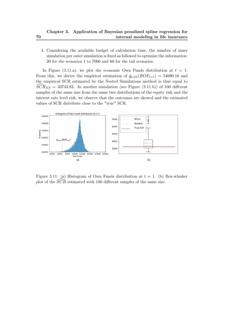
70Chapter 3. Application of Bayesian penalized spline regression for
internal modeling in life insurance
4. Considering the available budget of calculation time, the number of innersimulation per outer simulation is fixed as followed to optimize the information:20 for the scenarios 1 to 7000 and 60 for the tail scenarios.
In Figure (3.11.a), we plot the economic Own Funds distribution at t = 1.From this, we derive the empirical estimation of q0.5%(BOFt=1) = 54690.16 andthe empirical SCR estimated by the Nested Simulations method is thus equal toSCRNS = 33743.83. In another simulation (see Figure (3.11.b)) of 100 differentsamples of the same size from the same two distributions of the equity risk and theinterest rate level risk, we observe that the outcomes are skewed and the estimatedvalues of SCR distribute close to the "true" SCR.
Figure 3.11: (a) Histogram of Own Funds distribution at t = 1. (b) Box-whiskerplot of the SCR estimated with 100 different samples of the same size.
Chapter 4
Sparse group lasso additivemodeling for Pareto-type
distributions
Contents4.1 Part I - Overview of Extreme Values Theory . . . . . . . . . 72
4.1.1 Generalized extreme value distribution . . . . . . . . . . . . . 72
4.1.2 Peak-over-threshold method . . . . . . . . . . . . . . . . . . . 74
4.1.3 Example of limiting distributions . . . . . . . . . . . . . . . . 75
4.1.4 Statistical Estimation . . . . . . . . . . . . . . . . . . . . . . 77
4.1.5 Characterisation of Maximum Domains of Attraction . . . . . 79
4.2 Part II - Sparse group lasso additive modeling for condi-tional Pareto-type distributions . . . . . . . . . . . . . . . . . 79
4.2.1 Methodology . . . . . . . . . . . . . . . . . . . . . . . . . . . 80
4.2.2 Simulation Study . . . . . . . . . . . . . . . . . . . . . . . . . 89
4.3 Appendix . . . . . . . . . . . . . . . . . . . . . . . . . . . . . . 98
4.3.1 Proof of Lemma 1 . . . . . . . . . . . . . . . . . . . . . . . . 98
4.3.2 Best approximation by splines . . . . . . . . . . . . . . . . . 98
4.3.3 Block Coordinate Descent Algorithm . . . . . . . . . . . . . . 99
In extreme value statistics, estimation of the tail-index is of importance in nu-merous applications since it measures the tail heaviness of a distribution. Examplesinclude heavy rainfalls, big financial losses, high medical costs, just to name a few.When covariate information is available, we are mainly interested in describing thetail heaviness of the conditional distribution of the dependent variable given theexplanatory variables and the tail-index will be thus taken as a function of this co-variate information. In many practical applications, the explanatory variables cancontain hundreds of dimensions. Many recent methods use concepts of proximityin order to estimate model parameters based on their relation to the rest of thedata. However, in high dimensional space, the data is often sparse and the notionof proximity fails to retain its meaningfulness. Therefore, this implies deteriorationin estimation. Having this problematic, we aim to overcome this challenge in thecontext of the tail-index estimation given the explanatory variables.

72Chapter 4. Sparse group lasso additive modeling for Pareto-type
distributions
This chapter consists of two parts: The first part presents an overarching intro-duction of extreme values theory, which is served as base for our proposed method-ology. Then the mechanism of this methodology will be detailed in the second part.
4.1 Part I - Overview of Extreme Values Theory
Nowadays, modeling extreme events (hurricane, earthquake, floods, financial crises,oil shocks, etc.) is a particularly active research field. In recent years, there has beena growing interest in the application of Extreme Values Theory (EVT) for modelingsuch events.
Predict certain events or behaviors from the study of extreme values of a se-quence, is therefore one of the main goals for those trying to apply EVT. Thistheory emerged between 1920 and 1940, thanks to Frechet, Fisher and Tippett,Gumbel and Gnedenko. When modeling the maximum of a set of random variables,then, under certain conditions that we will specify later, its distribution can onlybelong to one of the three following laws: Weibull (with bounded support), Gumbel(with unbounded support and with fine tails) and Fréchet (with unbounded supportand thick tails). These three laws define a family of statistical distributions called"generalized extreme value distribution", whose applications are innumerable andvery diverse. We will limit ourselves in this report to related insurance risks.
The extreme values theory makes it possible to evaluate the rare events andthe losses associated with their appearance. In other words, when a significantloss occurs, this theory makes it possible to evaluate its magnitude. Moreover,this theory plays a particularly important role since it is directly interested in thetail of the distribution. In fact, only the extreme data are used to estimate theparameters of the EVT models which ensures a better fit of the model to the tailof the distribution and therefore a better estimate of the Value-at-Risk (VaR). VaRis a concept commonly used to measure the market risk of a portfolio of financialinstruments. It corresponds to the amount of losses that should only be exceededwith a given probability on a given time horizon.
In the following, the material is for the most part borrowed from [27]. Therefore,proofs are most often not given and readers are rather referred to the above referencesfor detailed proofs.
4.1.1 Generalized extreme value distribution
The extreme values theory aims to study the law of the maximum of a sequenceof real random variables even if, and especially if, the law of the phenomenon isunknown. Formally, let us consider (X1, . . . , Xn) a sequence of n independent andidentically distributed random variables of distribution function FX .
To study the behavior of extreme events, let us consider the random variableMn = max(X1, . . . , Xn). Since the random variables are independent and identically

4.1. Part I - Overview of Extreme Values Theory 73
distributed, then the distribution function of Mn is given by:
FMn(x) = P (Mn ≤ x) = P (X1 ≤ x; . . . ;Xn ≤ x) =
n∏i=1
P (Xi ≤ x) = FnX(x). (4.1)
Equation (4.1) is of very limited interest. Moreover, the law of a random variableX is rarely known precisely and, even if the law of this random variable is knownexactly, the law of the maximum term is not always easily calculable. For thesereasons, it is interesting to consider the asymptotic behaviors of the appropriatelystandardized maximum.
Definition: We say that two real random variables X and Y are of the sametype if there are two real constants a and b such that Y and aX + b follow the samelaw of distribution.
In a similar way to the central limit theorem, can we find normalization constantsan > 0 and bn and a non-degenerate law H such that:
P(Mn − bn
an≤ x
)= FnX(anx+ b)→ H(x) (4.2)
as n→∞ ?Fisher and Tippett [37] find a solution to this problem by means of a theorem
which bears their name and which is one of the foundations of the theory of extremevalues.
Theorem 1 (Fisher - Tippett Theorem). If there are two sequences of normalizationconstants with (an) > 0 and (bn) ∈ R and a non degenerate law of distribution H
such thatlimn→∞
FMn−bnan
(x) = H(x),
then H(x) is one of these three limits:
• Gumbel distribution: G0(x) = exp(− exp(−x)), x ∈ R
• Fréchet distribution: Φα(x) = exp (−x−α) I(0,∞)(x)
• Gumbel distribution: Ψα(x) = I[0,∞)(x) + exp (−(−x)α) I(−∞,0)(x).
Although the behavior of these laws of distribution is completely different, theycan be combined in a single parametrization containing a single parameter thatcontrols the thickness of the tail of distribution, which is called the tail-index ofextreme values:
Hγ(x) =
exp(−(1 + γx)
− 1γ
), if γ 6= 0; 1 + γx > 0
exp(− exp(−x)), if γ = 0
where H is a non-degenerate function. This law of distribution is called the gener-alized extreme values distribution (GEV). By introducing the location parameters

74Chapter 4. Sparse group lasso additive modeling for Pareto-type
distributions
µ and the dispersion σ into the parameterization, we obtain the most general formof the generalized extreme value distribution (GEV):
Hγ,µ,σ(x) = exp
(−(
1 + γx− µσ
)− 1γ
), γ 6= 0, 1 + γ
x− µσ
> 0 (4.3)
where γ is the shape parameter.The Fisher-Tippett Theorem provides the counterpart of the Central Limit The-
orem (CLT) in the case of extreme events. However, unlike the CLT, where the nor-mal distribution is the only possible limiting distribution. In the case of extremes,three types of limiting distribution are possible:
• Gumbel distribution: γ = 0,
• Fréchet distribution: γ > 0 corresponds to the Fréchet parameter α = 1γ ,
• Weibull distribution: γ < 0 corresponds to the Weibull parameter α = − 1γ .
The GEV-based approach has been criticized as the use of a single maximaleads to a loss of information contained in the other large values of the sample. Toovercome this problem, the Peak-over-Threshold method (POT) was introduced inPickands [89].
4.1.2 Peak-over-threshold method
The Peak-Over-Threshold (POT) method is based on the behavior of observed valuesbeyond a given threshold. In other words, it consists in observing not the maximumor the greatest values but all the values of the realizations which exceed a certainhigh threshold. The basic idea of this approach is to choose a sufficiently highthreshold and study the excesses beyond this threshold.
We define a threshold u ∈ R, Nu = cardi : i = 1, . . . , n,Xi > u, and Yj =
Xi−u > 0 for 0 ≤ j ≤ Nu where Nu is the number of exceedances over the thresholdu by the Xii=1,...,n and Yjj=1,...,Nu are the corresponding excesses.
We seek from the distribution FX to define a conditional distribution Fu withrespect to the threshold u for the random variables exceeding this threshold. Wethen define the conditional law of excess Fu by:
Fu(y) = P(X − u ≤ y |W > u) =FX(y + u)− FX(u)
1− FX(u)
The Pickands-Balkema-de Haan theorem [6,89] below gives the form of the limitingdistribution for extreme values: under certain convergence conditions, the limitingdistribution is a generalized Pareto distribution that we note GPD.
Theorem 2 (Pickands-Balkema-de Haan theorem). A distribution function F be-longs to the maximum domain of attraction of Hγ if and only if, there exists apositive function σ(u) such that:
limu→xF
sup0≤y≤xF−u
∣∣Fu(y)−Gγ,σ(u)(y)∣∣ = 0 (4.4)

4.1. Part I - Overview of Extreme Values Theory 75
where Fu is the conditional distribution function of the excesses for the threshold u,xF is the end point of FX , xF = supx ∈ R : FX(x) < 1 and Gγ,σ(u)(y) is theGPD given by:
Gγ,σ(u)(y) =
1−(
1 + γ yσ(u)
)− 1γ, if γ 6= 0
1− exp(− yσ(u)
), if γ = 0
(4.5)
with y ≥ 0 for γ ≥ 0 and 0 ≤ y ≤ −σ(u)γ for γ < 0.
This theorem shows the existence of a close relationship between the GPD andthe GEV (Generalized Extreme Value); Pickands [89] has shown that for any dis-tribution FX , the GPD approximation defined above is verified only if there arenormalization constants and a non-degenerate law such as Eq. (4.2) is satisfied. Inthis case, if H is written in the form of a GEV, then the tail index γ is the same asthat of the GPD.
Similarly, for the GPD, the case where γ > 0 corresponds to the distributionswith thick tails, for which 1 − G behaves like a power x−
1γ for x large enough. If
γ = 0, we have 1− exp(− yσ(u)
): it is an exponential law of parameter σ and finally
γ < 0, it is the type-II Pareto distribution with bounded support.The GPD has the following properties:
E(Y ) =σ
1− γ, γ < 1 (4.6)
V (Y ) =σ2
(1− γ)2(1− 2γ), γ <
1
2. (4.7)
In practice, the choice of the threshold constitutes a difficulty. In fact, u must belarge enough for the GPD approximation to be valid, but not too high to keepenough overruns to estimate model parameters. The threshold must be chosen soas to make a traditional arbitration between the bias and the variance.
Generally, u is determined graphically by exploiting the linearity of the meanexcess function e(u) for the GPD [34]. The function of average excess is given bythe relation:
e(u) = E (X − u | X > u) =σ + γu
1− γ, γ < 0.
This technique provides valuable help. However, one should not expect from it thegood value of u. In practice, several values of u must be tested. This problem ofchoice has aroused many works in the literature. Beirlant et al. [10] suggest choos-ing the threshold u that minimizes the asymptotic mean squared error of the Hillindex estimator, while assuming that FX belongs to Fréchet’s maximum attractiondomain.
4.1.3 Example of limiting distributions
In this subsection, we propose three examples illustrating how the limit distributionsof the GEV and the GPD manifest themselves in practice, taking into accountdifferent assumptions about the distribution FX .

76Chapter 4. Sparse group lasso additive modeling for Pareto-type
distributions
Exponential distribution
For the exponential law of parameter λ = 1, the distribution function is FX(x) =
1− e−x for x ≥ 0. By posing bn = ln(n) and an = 1 then,
FnX(anx+ b) =
(1− e−x
n
)n→ exp
(−e−x
)= G0(x) (4.8)
as n→∞.This shows that the normalized maximum (Mn − bn)/an of the exponential
distribution converges to Gumbel distribution. With regard to the POT method,taking σu = 1, then, for all y > 0,
Fu(y) =FX(y + u)− FX(u)
1− FX(u)
= 1− e−y.
Also, the limiting distribution is the GPD of parameter γ = 0 with σu = 1. Notethat in this case, the GPD is not simply the limiting distribution, but it is the exactdistribution for every u.
Pareto distribution
For the distribution function FX(x) = 1− cx−α, where c > 0 and α > 0. By posingbn = 0 and an = (nc)1/α then we have for x > 0:
FnX(anx+ b) =
(1− x−α
n
)n→ exp
(−x−α
)= Φα(x) (4.9)
which is the Fréchet distribution. Pareto distribution belongs to Fréchet’s domainsof attraction.
Based on the POT method with the threshold u and considering σu = ub forb > 0, then we have
Fu(y) =FX(u+ uby)− FX(u)
1− FX(u)
= 1− (1 + by)−α
which is the GPD with γ = 1/α and b = γ.
Normal distribution
Let FX(x) = 1√2π
∫ x−∞ e
−t2/2dt be the normal cumulative distribution function. Amathematical result says that 1 − F (x) ∼ 1
x√
2πe−x2/2in the neighborhood of +∞,
therefore:
limu→∞
1− FX (u+ z/u)
1− FX(u)= lim
u→∞
[(1 +
z
u2
)−1exp
(−1
2
(u+
z
u
)2+
1
2u2
)]= e−z
(4.10)

4.1. Part I - Overview of Extreme Values Theory 77
If we assume at first that βu = 1u , then
1− 1− FX(u+ z/u)
1− FX(u)=FX(u+ βuz)− FX(u)
1− FX(u)→ 1− e−z, u→ +∞
and subsequently the limiting distribution of the excesses beyond a threshold u isthe exponential distribution.
In a second time if we consider bn, the solution of the equation FX(bn) = 1− 1n ,
and an = 1bn, we obtain
n [1− FX(anx+ bn)] =1− FX(anx+ bn)
1− FX(bn)→ e−x.
And then
limn→∞
FnX(anx+ bn) = limn→∞
(1 +
e−x
n
)n→ exp
(−e−x
)= G0(x)
4.1.4 Statistical Estimation
Referring to the literature, various methods that have been proposed to estimate theparameters of the GEV and GPD laws are noted, the maximum likelihood method[103], the method of moments [24] the probability weighted moments method [4],or Bayesian methods [79]. There are also nonparametric approaches for estimatingthe tail index. The most used in practice are the Pickands estimator [89], the Hillestimator [53] (for the case of Frechet type laws only) and the Dekkers-Einmahl DeHann estimator [28]. The most popular method that under certain conditions is themost effective is the maximum likelihood method.
In what follows, we will first present this last parametric estimation method forthe GPD. Subsequently, we will present the value-at-risk estimate using an approachbased on the Peak Over Thershold (POT) method. And finally, we will presentanother non-parametric method, the McNeil and Frey [81] model that applies tofinancial data. For a more complete description, see Embrechts et al. [34].
4.1.4.1 Estimation of GPD parameters by maximum likelihood
Consider again the GPD whose the density function is given by:
g(y) =1
σ
(1 + γ
y
σ
)− 1γ−1
(4.11)
for y ≥ 0 if γ > 0, and 0 ≤ y ≤ −σξ if γ < 0.
The estimation of the GPD, by the method of maximum likelihood, relates tothe tail index γ as well as the scale parameter σ. The expression of the log-likelihoodis therefore
l(Y ; γ, σ) = −Nu ln (σ)−(
1 +1
γ
) Nu∑i=1
ln(
1 + γyiσ
)(4.12)

78Chapter 4. Sparse group lasso additive modeling for Pareto-type
distributions
for a sample of excesses Y = (y1, . . . , yNu). From this, by taking the derivatives withrespect to each parameter, we obtain the maximum likelihood estimator (MLE),from θ = (γ, σ).
For γ > −12 , Smith [101, 102], Hosking and Wallis [55] prove that the regular-
ity conditions of the likelihood function are fulfilled and the maximum likelihoodestimator results in an unbiased, asymptotically normal estimator.
4.1.4.2 Estimate of the Value-at-Risk or the extreme quantile
Recall that the distribution of excesses beyond sufficiently high threshold u is
Fu(y) = P (X − u ≤ y | X > u) =F (u+ y)− F (u)
1− F (u)=F (u)− F (u+ y)
F (u), y ≥ 0
(4.13)where F = 1− F . This can be rewritten as
Fu(y)F (u) = F (u)− F (u+ y). (4.14)
This is equivalent to
F (u+ y) = F (u)− Fu(y)F (u) = F (u)Fu(y). (4.15)
Thanks to the Pickands-Balkema-de Haan theorem, we have
Fu(y) ≈(
1 + γy
σ(u)
)− 1γ
, y ≥ 0 (4.16)
as u→∞. This approximation makes it possible to propose an estimator for Fu(y),which is of the form
ˆFu(y) =
(1 + γ
y
σ(u)
)− 1γ
. (4.17)
A natural estimate of F (u) is the empirical estimator
ˆFn(u) =1
n
n∑i=1
IXi>u =Nu
n(4.18)
where Nu is the number of exceedances.The estimator results from the tail F (u+ y) = F (x) (for) and therefore has the
form:ˆF (u+ y) = ˆFn(u) ˆFu(y) =
Nu
n
(1 + γ
y
σ(u)
)− 1γ
. (4.19)
By inverting this equation, we obtain the quantile estimator
xp = u+σ
γ
[(n
Nu(1− p)
)−γ− 1
](4.20)
for p > F (u). Finally, the Value-at-Risk (VaR) is nothing other than the extremequantile calculated from the asymptotic extreme distribution (Generalized ParetoDistribution), obtained by modeling extreme losses (or profits) by the POT method.

4.2. Part II - Sparse group lasso additive modeling for conditionalPareto-type distributions 79
4.1.5 Characterisation of Maximum Domains of Attraction
Before jumping into the second part of this chapter, let us recall the characterisationof maximum domains of attraction. However, we will mainly focus on the maximumdomain of attraction of Fréchet, or MDA(Fréchet), since we are only interested inheavy-detailed distributions. For more information, readers can refer to [95].
The characterisation of maximum domains of attraction actually relies on thetheory of regular-varying functions [16]. A positive function U is regularly-varyingwith index δ ∈ R at infinity if
limx→∞
U(λx)
U(x)= λδ (4.21)
for all λ > 0. This property is denoted by U ∈ RVδ.The following theorem (see Theorem 4 in [42]) tells us how the distribution
function F looks like if F belongs to MDA(Fréchet).
Theorem 3. F belongs to MDA(Fréchet) if and only if F = 1 − F is regularlyvarying with index −1/γ. The associated extreme-value index is γ. Moreover, apossible choice for the normalizing sequences is an = F←(1− 1/n) and bn = 0.
Let us highlight that necessarily the endpoint of F is infinite. The distributionF is called a Pareto-type distribution if F has the following form:
F (y) = 1− F (y) = y− 1γL(y), y > 0 (4.22)
for some slowly varying function L : (0,∞)→ (0,∞) measurable so that
L(λy)
L(y)→ 1 as y →∞, ∀λ > 0.
Interestingly, the theorem above shows that the all Pareto-type distributions belongto MDA(Fréchet).
4.2 Part II - Sparse group lasso additive modeling forconditional Pareto-type distributions
In the context of financial and actuarial modeling, the observations very often de-pend on the other parameters, such as business line, risk profile, seniority, etc.However, all these studies assume that the tail-index is constant regardless of thesevariables. Many recent studies, for example [23,117], emphasized that the tail-indexcould be function of these explanatory variables. But none of the previously men-tioned studies provide a way to estimate the tail-index parameter conditionally tothese variables. As far as we can tell, in the context of financial and actuarial mod-eling, only three studies have been undertaken to provide methods to estimate thetail-index parameter conditionally to covariates. Beirlant and Goegebeur [9] proposea local polynomial estimator in the case of a one-dimensional covariate. When the

80Chapter 4. Sparse group lasso additive modeling for Pareto-type
distributions
dimension of the covariate increases, this method becomes less effective since theconvergence rate of the estimator decreases rapidly. To improve the performanceof the estimator, a solution would be to increase the size of data, but this wouldbe problematic in practice since the database could not be easily enlarged. Then,Chavez-Demoulin et al. [22] propose an additive structure with spline smoothing toestimate the relationship between the GDP parameters and covariates. Recently,Heuchenne et al. [52] approach suggests a semi-parametric methodology to estimatethe tail-index parameter of a GPD.
In practice, many financial and actuarial data modeling problem may dependupon several explanatory variables, which might make direct tail-index parameterestimation less accurate, or even impossible. One technique to reduce dimension issparse group lasso, which was introduced by Simon et al. [100]. Motivated both bythe advances about the work of Chavez-Demoulin et al. [22] and the sparse grouplasso method, we investigate a variable-selecting method to estimate the tail-indexparameter conditionally to covariates.
Here is the section layout. We recall first some general results regarding thePeaks-over-Threshold (POT) methodology given covariates, and present the gener-alized additive model (GAM) in Section (4.2.1). In Section 4.2.1.4, we introducethe sparse group lasso regression and propose a computational algorithm, which isbuilt upon a theoretical property of our statistical model. Finally, we conduct asimulation study to assess the finite sample performance of the proposed methodin Section 4.2.2. At the end of this section, we carry out a comparative study withthe local polynomial estimation proposed by Beirlant and Goegebeur [9]. Someconcluding remarks are made in Section ??.
4.2.1 Methodology
4.2.1.1 Asymptotic conditional distribution in the POT technique
In this section, we will recall the POT method (see, for instance, [26, 75]) whencovariate information is available. Define a set of covariate X ⊂ Rp. In this paper,we assume that the design points xi = (x
(1)i , . . . , x
(p)i ) ∈ X for i = 1, . . . , n are fixed.
Let us consider (Yi,xTi )1≤i≤n where Yi is a random variable whose distributionfunction is of the form F (y|xi) = P (Yi ≤ y|xi) of the type (4.22) with some L(y|xi).Namely,
1− F (y|xi) = y−1/γ∗(xi)L(y|xi). (4.23)
Moreover, for some threshold function un(xi) > 0, we define the conditional distri-bution of Yi − un(xi) given Yi > un(xi) as follows :
Fun(xi)(z|xi) = P (Yi − un(xi) ≤ z|Yi ≥ un(xi)) =F (un(xi) + z|xi)− F (un(xi)|xi)
1− F (un(xi)|xi).
Gnedenko (see Theorem 4 in [42]) showed the equivalent between (4.23) andF (·|xi) ∈ D(Hγ∗(xi)). Then, according to the Pickands theorem [89], we have,

4.2. Part II - Sparse group lasso additive modeling for conditionalPareto-type distributions 81
for ∀i ∈ 1, . . . , n,
limun(xi)→∞
sup0≤z≤∞
|Fun(xi)(z|xi)−G (z; γ∗(xi), σ∗(xi))| = 0 (4.24)
where G(z; γ, σ) is the GPD. This means that, by taking un(xi) large enough, thedistribution of the excesses over un(xi) is sufficiently close to a GPD with the pa-rameters γ∗(xi) and σ∗(xi). Hence, we approximate the condition distribution ofYi−un(xi) given Yi > un(xi) by a GPD with the parameters γ∗(xi) and σ∗(xi) andall observations that exceed a specified high threshold are used to estimate γ∗(xi).However, since the conditional distribution of Yi − un(xi) given xi is not exactly aGPD, this consideration will imply a misspecification error in the estimation, whichis more difficult to assess.
To be more precise, let us denote by g(z; γ, σ) the density function of G(z; γ, σ)
being of the form
g(z; γ, σ) =1
σ
(1 + γ
z
σ
)− 1γ−1,
Let us define Mxi(γ, σ) = E(γ∗(xi),σ∗(xi)) [log g (Zi; γ, σ) |xi] the minus informationcross entropy [98] where Zi given xi exactly follows a GPD with the shape parametersγ∗(xi) and σ∗(xi) and E(γ∗(xi),σ∗(xi)) denotes the expectation with respect to thetrue parameters (γ∗(xi), σ∗(xi)). Clearly, we have
(γ∗(xi), σ∗(xi)) = arg max(γ,σ)∈R∗+×R∗+
Mxi(γ, σ) for every i = 1, . . . , n (4.25)
as a result of the Kullback–Leibler divergence [71] between g(z; γ, σ) andg(z; γ∗(xi), σ∗(xi)). Following the idea mentioned previously, we defineMun(xi)(γ, σ) = E [log g(Yi − un(xi); γ, σ)|xi, Yi ≥ un(xi)] the expectation of the ap-proximative log-likelihood log g(Yi − un(xi); γ, σ) given Yi > un(xi). Thanks to theequations (4.24) and (4.25), one can see that
(γ∗un(xi) (xi) , σ∗un(xi) (xi)
), which are
defined by(γ∗un(xi) (xi) , σ∗un(xi) (xi)
)= arg max
(γ,σ)∈R∗+×R∗+Mun(xi)(γ, σ), for every i = 1, . . . , n
are the approximations of (γ∗(xi), σ∗(xi)) for every i = 1, . . . , n. In order to obtainthe consistency and asymptotic normality of
(γ∗un(xi) (xi) , σ∗un(xi) (xi)
), we have to
impose a further condition on the behavior of the function L(y|xi) as follows.Condition (S): For every i = 1, . . . , n, L(tz|xi)
L(z|xi) = 1 + φ(z|xi)c(xi)∫ t
1 sρ(xi)−1ds+
o (φ(z|xi)) as z → ∞ for each t > 0, with φ(z|xi) > 0 and φ(z|xi) → 0 as z → ∞and ρ(z|xi) ≤ 0.
The above condition corresponds to the condition C.6 in Beirlant and Goegebeur[9]. Furthermore, this condition is equivalent to the second order condition (seeDefinition 2.3.1 and Theorem 2.3.9 in [27]). Under the second order condition,de Haan and Ferreira [27] showed that the asymptotic normality of the maximumlikelihood estimates holds for γ∗(xi) > −1
2 (please refer to Section 3.4 in [27] formore details).

82Chapter 4. Sparse group lasso additive modeling for Pareto-type
distributions
With a slight abuse of notation, we will use (γ∗(x), σ∗(x)) to represent themisspecified shape parameter (γ∗un(x)(x), σ∗un(x)(x)) for the rest of this paper.
4.2.1.2 Generalized Additive Model (GAM)
Recall that our main purpose is to describe the tail-heaviness of the conditionaldistribution of the dependent variable Y given the predictor x ∈ Rp. As consequence,the tail-index is taken as functions of the covariate x. As previously mentioned inthe introduction, Beirlant and Goegebeur [9] considered the POT approach andproposed the technique of local polynomial estimation to fit the shape parameter(γ∗(x), σ∗(x)) and their corresponding derivatives up to the degree of the chosenpolynomial. However, it is difficult to reproduce the forms of γ∗(x) and σ∗(x)
with high-dimensional covariates. This is the so-called "curse of dimensionality"problem, which is due to the fact that data points are isolated in their immensityand the notion of nearest points vanishes with such data. This thus implies therapid deterioration in convergence rate. On the other hand, the more regular γ∗(x)
and σ∗(x) are, the easier the regression functions are to estimate. The absence ofhypothesis on the form of the regression functions leads to a speed of convergencedepending on the number of explanatory variables. To overcome this difficulty, wecan make stronger assumptions about the form of γ∗(x) and σ∗(x), which brings usback to the case of parametric models and methods. However, these models lackflexibility for our problem.
Generalized additive models, introduced by Hastie and Tibshirani [49], can com-promise the flexibility of non-parametric models and the non-dependence of thespeed of convergence of estimators with respect to the number of components ofparametric models. Since γ∗(x) and σ∗(x) are positive functions, we then introduceour generalized additive model as follows:
γp,∞(x) = exp
γ0 +
p∑j=1
γj(x(j))
(4.26)
σp,∞(x) = exp
σ0 +
p∑j=1
σj(x(j))
(4.27)
where each additive function γj(·), σj(·)pj=1 belongs to the Sobolev space of con-tinuously differentiable functions. In order to ensure the identification we assumethat for every j = 1, . . . , p the additive functions γj , σj are centered, i.e.
n∑i=1
γj
(x
(j)i
)= 0,
n∑i=1
σj
(x
(j)i
)= 0 (4.28)
Supposing that log γ∗(x) and log σ∗(x) are additive will introduce a bias in theestimation, but this assumption is less restrictive than assuming a parametric formon the regression functions, so the modelling error is lower (see, for example [107],for more details about the additive approximation error).

4.2. Part II - Sparse group lasso additive modeling for conditionalPareto-type distributions 83
4.2.1.3 Natural cubic splines expansion
The model presented in (4.26) and (4.27) is still nonparametric and the estimationis therefore a problem of infinite dimension. We make it finite by expanding eachadditive functional components in natural cubic spline (NCS) bases with a reason-able amount of knots Kj for j = 1, . . . , p. Indeed, as pointed in Section 4.3.2, forany regular functions f , we can always find a best spline approximation f of f tominimize ‖f − f‖∞. The error in approximating f by f is usually small, thus inpractice we estimate f instead of f . An usual choice would be to use Kj − 4
√n
interior knots. For the sake of simplicity, we consider that every coupled-additivefunction (γj(·), σj(·))pj=1 will be expanded in the same base. Thus, we parametrize
γj(·) =
Kj∑k=2
θj,k
(hj,k(·)−
1
n
n∑i=1
hj,k
(x
(j)i
)), σj(·) =
Kj∑k=2
θ′j,k
(hj,k(·)−
1
n
n∑i=1
hj,k
(x
(j)i
))
where hj,k : R→ R+ is the natural cubic spline basis function constructed on the setof the predefined interior knots ξ(j)
1 , . . . , ξ(j)Kj satisfying ξ(j)
1 ≤ · · · ≤ ξ(j)Kj
. Namely,these natural cubic spline basis functions are of the form
hj,1(x) = 1, hj,2(x) = x, hj,k+2(x) = dk(x)− dKj (x) ∀k = 1, . . . ,Kj − 2
with dk(x) =(x−ξk)3
+−(x−ξKj )3+
ξKj−ξk. Clearly, this parametrization of the functional com-
ponents (γj(·), σj(·)) verifies the centering conditions given in (4.28). To simplifyour notation, let us define
hj,k(·) =
(hj,k(·)−
1
n
n∑i=1
hj,k
(x
(j)i
)), ∀j = 1, . . . , p, ∀k = 1, . . . ,Kj .
In the following, we denote by β0 and θ0 the intercept term instead of γ0 and σ0
to synchronize the notation with the coefficients θj,k, θ′j,k as presented previously.
Finally, our statistical model is defined as
γ(x) = exp
θ0 +
p∑j=1
Kj∑k=2
θj,khj,k
(x(j)) (4.29)
σ(x) = exp
θ′0 +
p∑j=1
Kj∑k=2
θ′j,khj,k
(x(j)) (4.30)
To sum up, the following diagram sets out the whole approximation scheme:

84Chapter 4. Sparse group lasso additive modeling for Pareto-type
distributions
4.2.1.4 Sparse group lasso estimation
For notational simplicity, we denote by ϕ =(θ0,θ
T , θ′0,θ
′,T)the entire parameter
vector where θ =(θT1 , . . . ,θ
Tp
)T , θ′ =(θ′,T1 , . . . ,θ
′,Tp
)Twith θj =
(θj,2, . . . , θj,Kj
)Tand θ′j =
(θ′j,2, . . . ,θ
′j,Kj
)Tfor every j = 1, . . . , p. This high-dimensional parame-
ter vector carries a group structure where the parameter is partitioned into disjointpieces. This usually occurs when dealing with expansions in high-dimensional addi-tive models as discussed in Section 4.2.1.2. The goal is high-dimensional estimationin generalized additive models being sparse with respect to whole group. Clearly, theparameter vector ϕ can be structured into groups G0,G1, . . . ,Gp and G0, G1, . . . , Gpwhich build a partition of the index set 1, . . . , 2 + 2
∑pj=1(Kj − 1). That is,
p⋃j=0
(Gj ∪ Gj) = 1, . . . , 2 + 2
p∑j=1
(Kj − 1)
and the intersection of any distinct groups is an empty set. Each of the groups isdefined in the following way:
θ0 = ϕG0 , θj = ϕGj , θ′0 = ϕG0
, θ′j = ϕGj , ∀j = 1, . . . , p.
Under this notation, the equations (4.29) and (4.30) can be rewritten as
γ(x|ϕ) = exp
p∑j=0
ϕGj hGj
(x(j)) (4.31)
σ(x|ϕ) = exp
p∑j=0
ϕGj hGj
(x(j)) (4.32)
with hG0(·) = hG0(·) = 1.
Let yi ∈ R be a realisation of Yi. We define in the sequel the empirical lossfunction as follows
Pnl(ϕ|un(·)) = − 1
n
n∑i=1
log g (yi − un(xi); γ(xi|ϕ), σ(xi|ϕ)) I(yi ≥ un(xi)). (4.33)
By minimizing this empirical loss function, we could obtain an estimate of the modelparameters ϕ. However, there are two main reasons why a practitioner is often notsatisfied with this estimating approach. The first reason is prediction accuracy: theestimators often have low bias but large variance, especially when p n. Shrinkingsome coefficients to 0 could improve the estimators quality. Indeed, we sacrificea little bias to reduce the variance of the estimators. This allows to balance thebias-variance trade-off which may improve the overall prediction accuracy. Thesecond reason is related to the interpretation. We prefer to bring out a smallersubset among a large number of predictors that exhibits the strongest effects. In

4.2. Part II - Sparse group lasso additive modeling for conditionalPareto-type distributions 85
other words, we would like to identify the principal explanatory variables having thestrongest impact on the determination of the tail index parameters. To this end,Yuan and Lin [120] suggested the group lasso penalty for this problem. Moreover,we would like not only sparsity of groups but also within each group. Indeed, thereare so many coefficients to calibrate in the model. By doing so it allows to omitnegligible coefficients and eliminate perturbative effects. Therefore, we combineboth the group lasso criterion and the l1 penalty proposed by Tibshirani [110].
Namely, for some constants λ1, λ2, µ1, µ2 > 0, defining
pen (ϕ|λ,µ) = λ1
p∑j=1
√Gj‖ϕGj‖2+λ2
p∑j=1
‖ϕGj‖1+µ1
p∑j=1
√Gj‖ϕGj‖2+µ2
p∑j=1
‖ϕGj‖1
(4.34)where Gj ≡ |Gj | = |Gj | denotes the cardinality of the group Gj , as well as of thegroup Gj , λ = (λ1, λ2)T and µ = (µ1, µ2)T .
The regression model that we consider to estimate (γ(x|ϕ), σ(x|ϕ)) is definedby
ϕ(un(·),λ,µ) = arg minϕ
Pnl(ϕ|un(·)) + pen (ϕ|λ,µ) . (4.35)
Note that this latter one is not exactly the penalized log-likelihood estimation sincethe true conditional distribution of Yi − un(xi) given Yi > un(xi) is not a GPD asmentioned in Section 4.2.1.1.
4.2.1.5 Algorithm for the sparse group lasso
In this section, we will use ϕ to designate the estimator ϕ(un(·),λ,µ) for nota-tional simplicity. Furthermore, for the later use, we need to define the followingparameters: sj = ϕGj/‖ϕGj‖2 if ϕGj 6= 0 (i.e. not equal to the 0-vector) and sj isa vector satisfying ‖sj‖2 ≤ 1 if ϕGj ≡ 0, and tj,k ∈ sign((ϕGj )k) if (ϕGj )k 6= 0 andtj,k ∈ [−1, 1] otherwise. By interchanging Gj with Gj , we obtain the similar defini-tion for uj and vj,k. Besides, we denote by ϕ−Gj the ϕ-vector whose componentsin Gj are set to zero, by ϕGj ,−k the ϕ-vector where only the kth component in thegroup Gj is set to zero.
For later use, let us denote by Φ a nonempty subset of R2(1+∑pj=1(Kj−1)) con-
taining the optimal vector of model parameters ϕ(un(·),λ,µ). As a consequenceof the Karush-Kuhn-Tucker (KKT) conditions (see, for example, [14]), we have thefollowing result, which is an important characterization of the optimal solution ϕin (4.35).
Lemma 1. Assume that Pnl(ϕ) is locally convex1 on Φ. Then, the necessary andsufficient conditions for ϕ to be a solution of (4.35) are
∂Pnl(ϕ)
∂ϕG0
= 0 (4.36)
1Regarding the definition of a locally convex function and its related details, readers can referto, for example, [76].

86Chapter 4. Sparse group lasso additive modeling for Pareto-type
distributions
∂Pnl(ϕ)
∂ϕG0
= 0 (4.37)
[∇Pnl(ϕ)Gj
]k
+ λ1
√Gj(sj)k + λ2tj,k = 0 (4.38)[
∇Pnl(ϕ)Gj
]k
+ µ1
√Gj(uj)k + µ2vj,k = 0 (4.39)
for every j = 1, . . . , p and k = 2, . . . ,Kj where ∇Pnl(ϕ)Gj (respectively for∇Pnl(ϕ)Gj ) denotes the gradient vector of Pnl(ϕ) with respect to ϕGj (respectivelyfor ϕGj ) at ϕ, and sj ,uj , tj,k, vj,k are defined above.
The proof of this lemma will be given in Appendix 4.3.1. These first deriva-tive tests (4.36 - 4.39) can give insight into the sparsity of groups and withineach group. Indeed, the necessary and sufficient condition for ϕGj ≡ 0 is thatthe equation
[∇Pnl(ϕ−Gj )Gj
]k
+ λ1
√Gj(sj)k + λ2tj,k = 0 has a solution with
‖sj‖2 ≤ 1 and tj,k ∈ [−1, 1] for every k ∈ Gj . To this end, we define J(tj ; ϕ−Gj ) =
1λ2
1Gj
∑k∈Gj
([∇Pnl(ϕ−Gj )Gj
]k
+ λ2tj,k
)2= ‖sj‖22. Let us denote by tj the mini-
mizer of J(tj , ϕ−Gj ). If J(tj , ϕ−Gj ) ≤ 1, then ϕGj ≡ 0. Otherwise, ϕGj is notidentically equal to the 0-vector. Moreover, it is easily seen that the minimizer is ofthe form:
tj,k =
−[∇Pnl(ϕ−Gj )Gj
]k
λ2, if |
[∇Pnl(ϕ−Gj )Gj
]k
λ2| ≤ 1
−sign([∇Pnl(ϕ−Gj )Gj
]k
), otherwise
(4.40)
With a little bit of algebra, we can show that J(tj , ϕ−Gj ) ≤ 1 is equivalent to
‖S(∇Pnl(ϕ−Gj )Gj , λ2
)‖2 ≤ λ1
√Gj
with S(·) the coordinate-wise soft thresholding operator:
(S (z, λ))i = sign(zi) (|zi| − λ)+ , z ∈ RGj , λ ∈ R+.
If ϕGj 6= 0, we apply the coordinate descent algorithm to find its element(ϕGj
)k.
The logic of the coordinate descent procedure is as follows: if(ϕGj
)k6= 0, then the
equation[∇Pnl(ϕ)Gj
]k
+ λ1
√Gj(ϕGj
)k/‖ϕGj‖ + λ2sign(
(ϕGj
)k) = 0 must have
a solution. This latter one leads to the inequality |(∇Pnl(ϕ)Gj
)k| > λ2. This
follows easily by examining the case where(ϕGj
)kis strictly positive and negative.
Therefore, check if |(∇Pnl(ϕGj ,−k)Gj
)k| ≤ λ2 and if so set
(ϕGj
)k
= 0. Otherwise,we minimize the equation (4.35) over (ϕGj )k by a one-dimensional optimization toget
(ϕGj
)k.
It is natural to think of a generalized gradient descent method to get the opti-mal solution. This consideration thus leads to the computation presented in 4.3.3.According to this algorithm, the optimal solution can be found by cycling throughthe groups G0 → G1 → · · · → Gp → G0. Within each iterative steps, we optimize theobjective function (4.35) by solving the equations (4.36 - 4.39) with respect to the

4.2. Part II - Sparse group lasso additive modeling for conditionalPareto-type distributions 87
current group Gj (or Gj) while keeping all except for the group fixed. This is calledthe block coordinate descend algorithm, as proposed by Friedman et al. [39].
As presented earlier, we considered the coordinate descent procedure to fit themodel within group. As pointed out by Simon et al. [100], this algorithm providesa poor performance in terms of timing and accuracy2. To overcome this drawback,they propose a block-wise descent algorithm which makes stride in performance.Inspired by this idea, we extend the fitting algorithm to our statistical model. Sinceour penalty (4.34) is separable between groups, we will only focus on an arbitraryone, saying Gj and the algorithm will be applied on the same principal for the others.Therefore, we consider the other group coefficients as fixed and ignore the penaltiescorresponding to these groups. With a slight abuse of notation, we denote in thefollowing our loss function Pnl(ϕGj ) taking ϕGj as parameter to minimize over.
We start with the majorization minimization scheme. This means that we ma-jorize the empirical loss function and then minimize the upper bound, together withthe penalty. Namely, the empirical loss function is majorized by
Pnl(ϕGj
)≤ Pnl
(ϕ0Gj
)+(ϕGj −ϕ0
Gj
)T.∇Pnl
(ϕ0Gj
)+
1
2t‖ϕGj −ϕ0
Gj‖22
where ϕ0Gj is a vector parameter to be determined at a later point and t is sufficiently
small so that the quadratic term dominates the Hessian of the loss function forevery ϕGj ∈ Φj with Φj the set of vectors parameter containing the target vector ofcoefficients.
We will omit the demonstration since it is given in [100]. Finally, we get that if‖S(ϕ0Gj − t∇Pnl(ϕ
0Gj ), tλ2
)‖2 ≤ tλ1
√Gj , then ϕGj ≡ 0. Otherwise,
ϕGj = F(ϕ0Gj , t) =
1−tλ1
√Gj
‖S(ϕ0Gj − t∇Pnl(ϕ
0Gj ), tλ2
)‖2
+
S(ϕ0Gj − t∇Pnl(ϕ
0Gj ), tλ2
)
To get the optimal solution, we cyclically iterate the procedure through the blocks.
At each iterative step, we update(ϕ0Gj
)(m)= ϕ
(m−1)Gj . By introducing a momentum
term in the gradient updates, Nesterov [83] showed that this modification can havea huge improvement in terms of convergence rate. As also suggested by Simon etal. [100], we present here Algorithm 1 for the blockwise descent fitting method.
4.2.1.6 Refitting step
A well-known drawback of l1-penalized estimators is the systematic shrinkage of thelarge coefficients towards zero. This may give rise to a high bias in the resultingestimators and may affect the overall conclusion about the model (see, for example,
2For the reason mentioned above, we will no longer discuss the performance of the Block Co-ordinate descent algorithm (or the accelerated generalized gradient descent algorithm) in the restof this paper. However, interested readers can can refer to Appendix 4.3.3 where the pseudo-codeversion of this algorithm is provided, in order to facilitate its implementation

88Chapter 4. Sparse group lasso additive modeling for Pareto-type
distributions
Algorithm 1 Block-wise Descent Algorithm1: Set up with the initial parameter vector ϕ(0) and the loop index m = 0.2: Increase m by one: m ← m + 1 and cycle the optimization procedure through
the groups:(2.1) Set ϕ(m) = ϕ(m−1).(2.2) Regarding j = 0, if ∇Pnl(ϕ(m)
−G0)G0 = 0: set ϕ(m)
G0= 0, and for j =
1, . . . , p, if ‖S(∇Pnl(ϕ(m)
−Gj )Gj , λ2
)‖2 ≤ λ1
√Gj : set ϕ(m)
Gj = 0. Otherwise, set
counter l = 1, step size t = 1 and ϕ(m,l)Gj = µ
(m,l)Gj = ϕ
(m)Gj and repeat the
following until convergence:(2.2.1) Update gradient g = ∇Pnl
(ϕ
(m,l)Gj
).
(2.2.2) Estimate optimal step size by iterating t← 0.8 ∗ t until
Pnl(F(ϕ
(m,l)Gj , t)
)≤ Pnl
(ϕ
(m,l)Gj
)+(
∆(m,l)t
)T.g +
1
2t‖∆(m,l)
t ‖22
with ∆(m,l)t = F(ϕ
(m,l)Gj , t)− ϕ(m,l)
Gj .
(2.2.3) Update µ(m,l)Gj by µ(m,l+1)
Gj ← F(ϕ(m,l)Gj , t).
(2.2.4) Update ϕ(m,l) by
ϕ(m,l+1) ← µ(m,l)Gj +
l
l + 3
(µ
(m,l+1)Gj − µ(m,l)
Gj
).
(2.2.5) Increase l by one: l← l + 1.(2.3) Repeat the procedure for the groups Gj for j = 0, . . . , p.
3: Repeat the entire step (2) until convergence.

4.2. Part II - Sparse group lasso additive modeling for conditionalPareto-type distributions 89
[11]). A simple remedy is to treat sparse group lasso as a variable selection tool andto perform a refitting step on the select support. Namely, let us define the activeset by
SG = (j, k)|ϕGj,k 6= 0, SG = (j, k)|ϕGj,k 6= 0
Next, we define
γ′(x|ϕ) = exp
∑(j,k)∈SG
ϕGj,k hGj,k
(x(j)) (4.41)
σ′(x|ϕ) = exp
∑(j,k)∈SG
ϕGj,k hGj,k
(x(j)) (4.42)
Our refitted estimator is thus the only minimizer of the following equation
ˆϕ = arg minϕ
Pnl′(ϕ|un(·)) (4.43)
where
Pnl′(ϕ|un(·)) = − 1
n
n∑i=1
log g(yi − un(xi); γ′(xi|ϕ), σ′(xi|ϕ)
)Iyi ≥ un(xi).
4.2.2 Simulation Study
How well does the sparse group lasso procedure described above estimate the tail-index function γ∗(x)? To answer this question, we conduct a small simulationstudy of the block-wise descent estimator where yini=1 are generated from theBurr(η, τ(x), ξ) distribution [21] for which the distribution function is given by
FBurr(y) = 1−(
η
η + yτ(x)
)ξ. (4.44)
Let us recall the Hall class of Pareto-type distributions [46] which is of the form
1− F (y) = ay− 1γ∗ (x)
[1 + by−θ(x) + o
(y−θ(x)
)].
Note that this class of distribution satisfies the condition 1 with c(x) = −θ(x)b,ρ(x) = −θ(x) and φ(z|x) = z−θ(x). It is easily seen that the Burr(η, τ(x), ξ) distri-bution belongs to the Hall class of Pareto-type distribution with γ∗(x) = 1/(ξτ(x)),a = ηξ, b = −ηξ and θ(x) = τ(x) since its survival function can be written as
1− FBurr(y) = y−ξτ(x)ηξ(
1− ξηy−τ(x) + o(y−τ(x)))
as y → ∞. Therefore, the condition (S) is satisfied with c(x) = ηξτ(x), ρ(x) =
−τ(x) and φ(z|x) = z−τ(x).In this simulation study, we consider two sample sizes n = 500, 5000 and two p
values p = 2 and 10. Usually in many high-dimensional studies, the dimension of

90Chapter 4. Sparse group lasso additive modeling for Pareto-type
distributions
the data vectors p is comparable or may be larger than the sample size n. Hence, itis obvious that our setting with p = 10 can not be considered as high dimensionalcovariate. However, we realized that it becomes computationally expensive in termsof running time required to perform estimation when the dimensionality increases.Therefore, in this paper, we limit ourselves to the case p = 10. Surprisingly, we notethat the proposed methodology slightly outperforms the local polynomial maximumlikelihood regression proposed by Beirland and Goegebeur [9] even with p = 10.
The data are generated from the Burr(η, τ(x), ξ) distribution with ξ = η = 1
andτ(x) =
20
3[(x(1))2 − (x(2))2 + 4
]where x =
(x(1), x(2)
)T for p = 2 and x =(x(1), x(2), . . . , x(10)
)T for p = 10. Clearly,there are only two active variables for both cases. From this, it follows that the tail-index function γ∗(x) is then given by
γ∗(x) =1
ξτ(x)= 0.15
[(x(1))2 − (x(2))2 + 4
]. (4.45)
Each explanatory variable x(j), j = 1, . . . , 10 takes value from the 10-equally spacedsamples in the closed interval [0, 1]. For each simulated dataset, we apply the pro-posed methods to estimate γ∗(x).
A hurdle in the Peaks-over-threshold approach for analyzing extreme values isthe selection of the threshold. The misdetermination of the threshold value willhave a non negligible impact on the performance of the estimator. Indeed, thresholdselection constitutes a trade-off situation between bias and variance. If we set thethreshold value too low, the GPD approximation is not suitable which implies a largebias. On the other hand, if we set the threshold value too high, a small numberof observations is used which leads to an increasing variance in the estimated GPDparameters. In the previous section, one considers that threshold un(x) depends onboth the covariates x and the sample size n, with un(x)→∞ as n→∞. However,this ideal threshold selection framework will be addressed in this section since it goesbeyond the scope of our paper. Hence, we assume that the threshold is constant interms of the explanatory variables x, but still depends the sample size.
Instead of the regularization parameters (λ1, λ2, µ1, µ2) as in (4.34), we considera modification which allows for more efficient computation. Namely, we take λ1 =
(1 − α1)λ, λ2 = α1λ, µ1 = (1 − α2)µ and µ2 = α2µ where α1, α2 ∈ [0, 1] are themixing parameters − a convex combination of the lasso and group lasso penalties.In practice, cross-validation or generalized cross-validation has been widely used tosearch for the optimal tuning parameters λ, µ, α1, α2 and the threshold u in order tomaximize its performance. However, since there are too many tuning parameters,this calibration process could be a computational burden and hardly be useful formany practical applications. Therefore, we consider the reduction of the "degreesof freedom" by taking α1 = α2 = α. Furthermore, since we expect strong group-wise sparsity, we would thus use α = 0.05. This condition clearly does not give
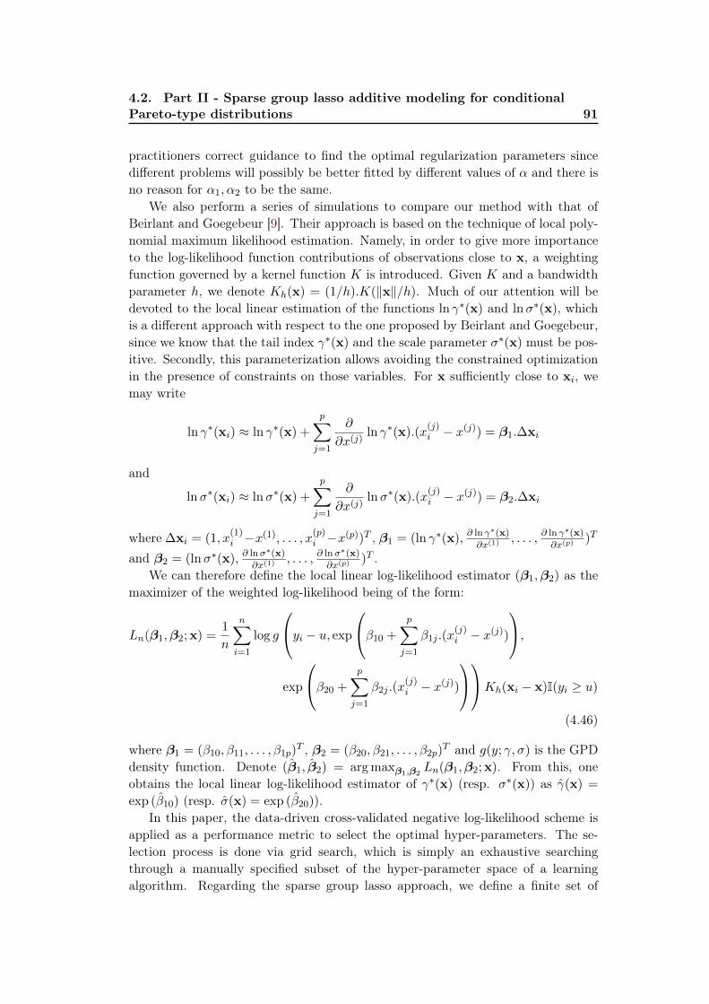
4.2. Part II - Sparse group lasso additive modeling for conditionalPareto-type distributions 91
practitioners correct guidance to find the optimal regularization parameters sincedifferent problems will possibly be better fitted by different values of α and there isno reason for α1, α2 to be the same.
We also perform a series of simulations to compare our method with that ofBeirlant and Goegebeur [9]. Their approach is based on the technique of local poly-nomial maximum likelihood estimation. Namely, in order to give more importanceto the log-likelihood function contributions of observations close to x, a weightingfunction governed by a kernel function K is introduced. Given K and a bandwidthparameter h, we denote Kh(x) = (1/h).K(‖x‖/h). Much of our attention will bedevoted to the local linear estimation of the functions ln γ∗(x) and lnσ∗(x), whichis a different approach with respect to the one proposed by Beirlant and Goegebeur,since we know that the tail index γ∗(x) and the scale parameter σ∗(x) must be pos-itive. Secondly, this parameterization allows avoiding the constrained optimizationin the presence of constraints on those variables. For x sufficiently close to xi, wemay write
ln γ∗(xi) ≈ ln γ∗(x) +
p∑j=1
∂
∂x(j)ln γ∗(x).(x
(j)i − x
(j)) = β1.∆xi
and
lnσ∗(xi) ≈ lnσ∗(x) +
p∑j=1
∂
∂x(j)lnσ∗(x).(x
(j)i − x
(j)) = β2.∆xi
where ∆xi = (1, x(1)i −x(1), . . . , x
(p)i −x(p))T , β1 = (ln γ∗(x), ∂ ln γ∗(x)
∂x(1) , . . . , ∂ ln γ∗(x)
∂x(p) )T
and β2 = (lnσ∗(x), ∂ lnσ∗(x)
∂x(1) , . . . , ∂ lnσ∗(x)
∂x(p) )T .We can therefore define the local linear log-likelihood estimator (β1,β2) as the
maximizer of the weighted log-likelihood being of the form:
Ln(β1,β2;x) =1
n
n∑i=1
log g
yi − u, exp
β10 +
p∑j=1
β1j .(x(j)i − x
(j))
,exp
β20 +
p∑j=1
β2j .(x(j)i − x
(j))
Kh(xi − x)I(yi ≥ u)
(4.46)
where β1 = (β10, β11, . . . , β1p)T , β2 = (β20, β21, . . . , β2p)
T and g(y; γ, σ) is the GPDdensity function. Denote (β1, β2) = arg maxβ1,β2
Ln(β1,β2;x). From this, oneobtains the local linear log-likelihood estimator of γ∗(x) (resp. σ∗(x)) as γ(x) =
exp (β10) (resp. σ(x) = exp (β20)).In this paper, the data-driven cross-validated negative log-likelihood scheme is
applied as a performance metric to select the optimal hyper-parameters. The se-lection process is done via grid search, which is simply an exhaustive searchingthrough a manually specified subset of the hyper-parameter space of a learningalgorithm. Regarding the sparse group lasso approach, we define a finite set of

92Chapter 4. Sparse group lasso additive modeling for Pareto-type
distributions
"reasonable" values for u, λ and µ as follows u ∈ 0.0, 0.1, . . . , 3.9, 4.0, λ, µ ∈10−2.0, 10−2.1, . . . , 10−3.3, 10−3.4. Similarly, we set u ∈ 0.0, 0.1, . . . , 3.9, 4.0 andh ∈ 101, 101.05, . . . , 102 for the local polynomial approach.
On each knot, we compute the 5-fold cross validation error which is defined asfollows:For the sparse group lasso approach:
CVSGL(λ, µ;u) =1
5
5∑k=1
CV [k](λ, µ;u) (4.47)
For the local polynomial approach:
CVLP(h;u) =1
5
5∑k=1
CV [k](h;u) (4.48)
where CV [k](λ, µ;u) as well as CV [k](h;u) is the cross-validation er-ror in predicting the kth part (testing set), which is given by−
∑i∈testing
set
log g(yi − u; γ[−k](xi), σ[−k](xi)
)I(yi ≥ u) with g(y; γ, σ) the GPD
density function, γ[−k], σ[−k] calibrated on the training set.The use of (4.47) is illustrated in Figure 4.1 for n = 5000 and p = 10 where we
denote by CVoptimal(u) = minλ,µCV (λ, µ;u) the optimal cross validation metricsgiven the threshold u.
Figure 4.1: (left) CVoptimal(u) = minλ,µCV (λ, µ;u) versus the threshold u; (right)Contour plot of 5-fold CV error as a function of λ and µ at u = 1 and α = 0.05 forn = 5000 and p = 10.
Regarding the sparse group lasso estimation, we are also interested in how wellwe can estimate the non-zero patterns of the κj ’s with others observations. To thisend, we repeat such a procedure a total of 100 times with 100 independent samplesof size n = 5000 for p = 10. In theory, we have to re-evaluate the optimal hyper-parameters u, λ and µ for each scenario since all these parameters depend upon the

4.2. Part II - Sparse group lasso additive modeling for conditionalPareto-type distributions 93
number of exceedances over threshold. However, in practice, this latter step requiresmultiple iterative calculations which could be a computational burden. Therefore,for sake of simplicity, we assume that the optimal hyper-parameters remain constantwith respect to different scenario. However, we would like to note that in sometrials we were unable to make the sparse-group lasso regression select the right zerocoefficients. This is due to the misspecified optimal hyper-parameters and the idealthreshold value with respect to the given sample, and due to the grouping effects.Overall we found that the sparse-group lasso reaches about 62% prediction accuracy,which is the proportion of correct nonzero functional components identifications overthe initial total number of samples, i.e. 100.
Once the optimal hyper-parameters for the sparse group lasso estimation and thelocal polynomial estimation have been calibrated, our final step consists in check-ing how well these estimations perform. For this purpose, we compute the MeanIntegrated Squared Error (MISE) which is defined as
MISE =
∫[0,1]p
MSE(x)dx (4.49)
where we denote by MSE(x) = empirical mean of∣∣γ (x; xini=1, y
(k)i ni=1
)−
γ∗(x)∣∣2 : 1 ≤ k ≤ 100
the (empirical) mean squared error at point x ∈ [0, 1]p. As
a reminder, the mean squared error allows us, in a single measurement, to capturethe ideas of bias and variance in our models, as well as showing that there is someuncertainty in our models that we cannot get rid. Therefore, the mean squarederror is arguably the most important criterion used to evaluate the performance ofan estimator at a particular point and the Mean Integrated Squared Error is thusconsidered as global metric for the performance of an estimation method. To valuethe equation (4.49) is a difficult operation, we will thus replace it by its roughlyapproximated version being of the form
MISE = ∆px5∑
m1=1
5∑m2=1
∑m3∈1,2
· · ·∑
mp∈1,2
MSE(x(1)m1, . . . , x(p)
mp) (4.50)
where x(j)mj takes values in 0, 0.25, 0.5, 0.75, 1 for j = 1, 2 and 0.25, 0.75 for
j = 3, . . . , p, ∆px = (0.25)2.(0.5)p−2. As can be seen, the discretization is moregranular with respect to the first two explanatory variables in (4.50) since these aretwo active variables in our model (4.45). Our key findings are reported in Table 1.
Surprisingly, we find that the thresholds u for different settings, obtained byusing the cross-validation optimization method (4.47, 4.48) are more or less the samelevels whether the local polynomial approach or the sparse group lasso approach.As observed from our numerical studies, the time required to calculate the cross-validation metrics in the sparse group lasso approach is much more longer than thatin the local polynomial approach. This result tells us that the optimal thresholdobtained from the criterion (4.48) could be directly applied in the sparse group lasso

94Chapter 4. Sparse group lasso additive modeling for Pareto-type
distributions
LocalPolynom
ialSparse
Group
Lasso
pn
uh
MISE
(Std)(×
10−
2)u
λµ
MISE
(Std)(×
10−
2)
5000.8
103
4.82
(2.08)0.5
0.5×
10−
30.63×
10−
36.22
(3.37)
2
5000
1.5
101.3
0.76
(0.47)1.5
0.5×
10−
30.63×
10−
31.44
(0.65)
5000.5
104
8.54
(0.42)0.5
5.01×
10−
35.01×
10−
36.81
(4.31)
10
5000
1.0
100.8
2.75
(0.59)1.0
1.58×
10−
32.0×
10−
31.56
(0.75)
Table
4.1:Sum
mary
ofoptim
alhyper-param
eters,as
well
asthe
approximated
Mean
IntegratedSquared
Error
MISE,
forthe
localpolynom
ialestim
ationand
thesparse
grouplasso
estimation,
with
respectto
differentsettings
(p=
2,10
andn
=500,500
0).To
measure
howspread
outthe
calculationof
MISE
is,we
compute
itscorrespond-
ingstandard
deviation(Std),
which
isthe
squareroot
ofthe
numerical
valueobtaine
while
calculatingvar (MISE )
=
∆px ∑
5m1=
1 ∑5m
2=
1 ∑m
3 ∈1,2 ··· ∑
mp ∈1,2var (MSE
(x(1
)m
1 ,...,x(p
)mp ) ).

4.2. Part II - Sparse group lasso additive modeling for conditionalPareto-type distributions 95
estimation, or at least as an indicator to check or to reinforce the reliability of theoptimal threshold obtained from the criterion (4.47).
Table 1 shows that the local polynomial estimation has a better fit for low di-mensional data (p = 2). The explanation of these results is twofold. First, thelocal polynomial estimation for low dimensional data is less subject to the curse ofdimensionality (reference). Second, except for the GDP approximation (4.24), thereis no any other approximation error that could occur. This is however not the casefor the sparse group lasso estimation where we consider the natural cubic splineapproximation (4.29, 4.30) even though these approximation errors could be small.This thus results in a better performance of the local polynomial estimation for lowdimensional data. By contrast, the sparse group lasso estimation globally gives abetter result for high dimensional data (p = 10). Clearly, in this case, the local poly-nomial estimation is affected by the curse of dimensionality, caused by the sparsityof data in a high dimensional space, resulting in a decrease in fastest achievable rateof convergence. As a result, this leads to a bad performance for the local polynomialestimators. The natural cubic spline assumption and the sparse group lasso algo-rithm could prevent those estimators suffering from the curse of dimensionality bypartially or totally eliminating the non-active explanatory variables. As mentionedin Section (4.2.1.6), imposing a penalty term based on the l1-norm will generate ahigh bias in our estimators. This latter one implies an increase in estimation errors.Therefore, we need to re-calibrate the coefficients on the active set. Besides, if wefocus on the last column in Table 1, we will observe that the MISE for p = 10 isslightly greater than the MISE for p = 2 whether n = 500 or 5000. As explainedabove, these prediction inaccuracies come from the fact that the sparse group lassomethod is somehow not able to identify all the non-active coefficients. Consequently,this drawback will create a small fluctuation in our estimators.
So far we compare the (rougly approximated) mean integrated squared errorcalculated by the local polynomial approach to that calculated by the sparse grouplasso approach with different settings. In the following we carry out the out-of-sample test to elaborate the efficiency and forecasting capability of our estimatorsat different points with the same settings. As it involves only two active explanatoryvariables (x(1), x(2)) constituting a two dimensional plane [0, 1] × [0, 1], This planeis divided into four quadrants. The first quadrant is the upper left-hand cornerof the plane [0, 0.5] × [0.5, 1]. The second quadrant is the upper right-hand corner[0.5, 1]× [0.5, 1]. The third quadrant is the lower left-hand corner [0, 0.5]× [0, 0.5].Finally, the fourth quadrant is the lower right-hand corner [0.5, 1]× [0, 0.5]. At eachquadrant, we take unintentionally a testing point as shown in Table 2. For p = 10,we will concatenate the active part (x(1), x(2)) and the inactive part x−(1,2) ∈ R8.Let us define u+ = (0.15, 0.25, 0.35, . . . , 0.85)T and u− = (0.85, 0.75, 0.65, . . . , 0.15).The inactive part x−(1,2) will take value in either u+ or u−. Finally we come upwith 4 testing points as shown in Table 2 for p = 10. In this study, we will focuson the coverage probability and the average of confidence intervals at these testingpoints. Recall that the coverage probability is the proportion of the time that the

96Chapter 4. Sparse group lasso additive modeling for Pareto-type
distributions
confidence interval contains the true value. To this end, we proceed the simulationas follows:
1. Reuse the samples of size n = 100, which are generated in the MISE calcu-lation, i.e.
y(k)i ni=1 : 1 ≤ k ≤ 100
.
2. Compute the 95% confidence interval (CI) for each sample by applying theboostrap sampling with replacement method from nboot = 500 boostrappeddata sets (see, for example, [29]).
3. Compute the proportion of samples for which the true tail index γ∗(x) iscontained in the confidence interval. That proportion is an estimate for theempirical coverage probability for the CI.
4. Compute the average of confidence intervals CI.
Why is this necessary? Isn’t the coverage probability always 95%? The answeris negative since the estimators
γ(x; xi)ni=1, y
(k)i ni=1) : 1 ≤ k ≤ 100
are not
normally distributed and the sample sizes are not large enough that we can invokethe Central Limit Theorem. Finally, our key findings are reported in Table 2.
N = 500, p = 2
Local Polynominal Sparse Group Lasso
Coverage Probability CI Coverage Probability CI
(0.12, 0.86) 35% 0.2306 44% 0.361
(0.76, 0.21) 53% 0.4082 90% 0.5612
(0.22, 0.01) 46% 0.5097 64% 0.6843
(0.92, 0.96) 10% 0.3673 58% 0.597
N = 500, p = 10
Local Polynominal Sparse Group Lasso
Coverage Probability CI Coverage Probability CI
(0.12, 0.86, u+) 0% 0.049 44% 0.3924
(0.76, 0.21, u+) 0% 0.049 4% 0.361
(0.22, 0.01, u−) 1% 0.1009 0% 0.025
(0.92, 0.96, u−) 0% 0.025 19% 0.3619
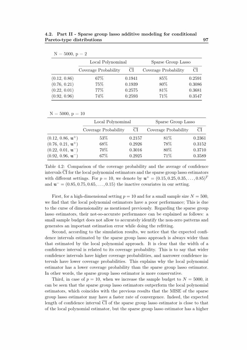
4.2. Part II - Sparse group lasso additive modeling for conditionalPareto-type distributions 97
N = 5000, p = 2
Local Polynominal Sparse Group Lasso
Coverage Probability CI Coverage Probability CI
(0.12, 0.86) 67% 0.1941 85% 0.2591
(0.76, 0.21) 75% 0.1939 80% 0.3086
(0.22, 0.01) 77% 0.2575 81% 0.3681
(0.92, 0.96) 74% 0.2593 71% 0.3547
N = 5000, p = 10
Local Polynominal Sparse Group Lasso
Coverage Probability CI Coverage Probability CI
(0.12, 0.86, u+) 53% 0.2157 81% 0.2361
(0.76, 0.21, u+) 68% 0.2926 78% 0.3152
(0.22, 0.01, u−) 70% 0.3016 80% 0.3710
(0.92, 0.96, u−) 67% 0.2925 71% 0.3589
Table 4.2: Comparison of the coverage probability and the average of confidenceintervals CI for the local polynomial estimators and the sparse group lasso estimatorswith different settings. For p = 10, we denote by u+ = (0.15, 0.25, 0.35, . . . , 0.85)T
and u− = (0.85, 0.75, 0.65, . . . , 0.15) the inactive covariates in our setting.
First, for a high-dimensional setting p = 10 and for a small sample size N = 500,we find that the local polynomial estimators have a poor performance; This is dueto the curse of dimensionality as mentioned previously. Regarding the sparse grouplasso estimators, their not-so-accurate performance can be explained as follows: asmall sample budget does not allow to accurately identify the non-zero patterns andgenerates an important estimation error while doing the refitting.
Second, according to the simulation results, we notice that the expected confi-dence intervals estimated by the sparse group lasso approach is always wider thanthat estimated by the local polynomial approach. It is clear that the width of aconfidence interval is related to its coverage probability. This is to say that widerconfidence intervals have higher coverage probabilities, and narrower confidence in-tervals have lower coverage probabilities. This explains why the local polynomialestimator has a lower coverage probability than the sparse group lasso estimator.In other words, the sparse group lasso estimator is more conservative.
Third, in case of p = 10, when we increase the sample budget to N = 5000, itcan be seen that the sparse group lasso estimators outperform the local polynomialestimators, which coincides with the previous results that the MISE of the sparsegroup lasso estimator may have a faster rate of convergence. Indeed, the expectedlength of confidence interval CI of the sparse group lasso estimator is close to thatof the local polynomial estimator, but the sparse group lasso estimator has a higher
98Chapter 4. Sparse group lasso additive modeling for Pareto-type
distributions
coverage probability.
4.3 Appendix
4.3.1 Proof of Lemma 1
The conditions (4.36) and (4.37) are trivial. To prove (4.38) and (4.39), we first recallthe definition of the subgradient and subdifferential of a locally convex function on Ω,f : Ω→ R, at x ∈ Ω where Ω is a nonempty subset of Rm. A vector d ∈ Rm is calleda subgradient of f at point x if f(y) ≥ f(x)+(y−x)T .d for all y ∈ Ω. The collectionof all subgradients of f at x is called the subdifferential of f at x, denoted by ∂f(x).Then, a neccesary and sufficient conditions for x to be a minimum of f is that0 ∈ ∂f(x). For any further information about the subgradient and subdifferentialas well as the optimality theorem, the interested readers can refers to [14]. Let usreturn to our proof. We can easily verify (the same arguments for the groups Gj)that
∂‖ϕGj‖2 = e ∈ RGj ; e =ϕGj‖ϕGj‖2
if ϕGj 6= 0 and ‖e‖2 ≤ 1 if ϕGj ≡ 0.
And the subdifferential set for |(ϕGj )k| obviously equals
∂|(ϕGj )k| = t ∈ R; t = sign((ϕGj )k) and |t| ≤ 1 if (ϕGj )k = 0
Due to local convexity and differentiability of Pnl(ϕ), we obtain finally the condi-tions (4.38) and (4.39).
4.3.2 Best approximation by splines
Let us first introduce two functional spaces.
Definition 1 (Polynomial Spline Space Φa,bs ). Letting ξl for l ∈ 1, . . . ,K be K-
interior knots satisfying the condition a = ξ0 ≤ ξ1 ≤ · · · ≤ ξK+1 = b. We define Φa,bs
the space of functions whose element is a polynomial of at most degree p on each ofthe intervals [ξl, ξl+1) for l = 0, 1, . . . ,K and is p− 1 continuously differentiable on[a, b] if p ≥ 1.
Definition 2 (Empirically Centered Polynomial Spline Space Φa,bs ). Given the de-
sign points (x1, . . . , xn) ∈ [a, b]n, a polynomial spline space is centered if for everyg ∈ Φa,b
s the following identity holds:
1
n
n∑i=1
g(xi) = 0.
We denote by Φa,bs the empirically centered polynomial spline space.

4.3. Appendix 99
According to de Boor (p. 149 in [18]), for every f(x) ∈ Cp+1([a, b]), there exists aconstant c > 0 and a spline function f ∈ Φa,b
s , such that ‖f− f‖∞ ≤ c‖f (p+1)‖∞δp+1
with δ = max1≤l≤K(ξl+1 − ξl).Given the design points (x1, . . . , xn) ∈ [a, b]n, we assume furthermore that
1
n
n∑i=1
f(xi) = 0.
By defining f(x) = f(x) − 1n
∑ni=1 f(xi) ∈ Φa,b
s , it is straightforward to show thatthere exists a positive constant c′ such that ‖f − f‖∞ ≤ c′‖f (p+1)‖∞δp+1.
4.3.3 Block Coordinate Descent Algorithm
Algorithm 21: Set up with the initial parameter vector ϕ(0) and the loop index m = 0.2: Increase m by one: m ← m + 1 and cycle the optimization procedure through
the groups:(2.1) Set ϕ(m) = ϕ(m−1).(2.2) Regarding j = 0, if ∇Pnl(ϕ(m)
−G0)G0 = 0: set ϕ(m)
G0and for j = 1, . . . , p,
if ‖S(∇Pnl(ϕ(m)
−Gj )Gj , λ2
)‖2 ≤ λ1
√Gj : update ϕ(m)
Gj = 0. Otherwise, cyclethe optimization procedure with respect to each coordinate within the groupfixed. That is, if |
(∇Pnl(ϕ(m)
(Gj ,−k))Gj
)k| ≤ λ2: update (ϕ
(m)Gj )k = 0. Otherwise,
minimize the objective function over (ϕGj )k by a one-dimensional optimization.Cyclically iterate this coordinate-wise optimization process until convergence.
(2.3) Repeat the procedure for the groups Gj for j = 0, . . . , p.3: Repeat the entire step (2) until convergence.


Chapter 5
Conclusion
The objective of this thesis is twofold. Firstly, we aim to define the SCR estimationerror related to the use a proxy in the context of the Solvency II regime, to establishthe various causes of this error and to propose a methodology allowing it to bequantified in order to assess and control it.
Namely, we suggest to decompose the loss function into marginal and residualloss functions and apply the Bayesian penalized spline smoothing analysis on eachfunctional components and showed how to control its errors. We also carried outseveral numerical tests on a simplified life insurance ALM simulator aiming to putinto practice this methodology of quantification of the model error and the result isconsidered satisfactory. But, how well does this method perform with respect to theothers in low and high dimensions (number of underlying risk-factors)? The optimalrate of convergence is typically of the form Γ−2r where r = p/(2p+ d), Γ being theavailable sampling budget, p being a measure of the assumed smoothness of the lossfunction, d being the dimension of underlying risk-factors. The rate of convergencebecomes slower when d increases. This is caused by the sparsity of data in high-dimensional spaces, resulting in a decrease in fastest achievable rates of convergenceof regression function. This phenomenon is called the "curse of dimensionality". Inthe context of portfolio risk measurement, Hong et al. [54] in particular show thesame issue of non-parametric approaches in high dimensional settings.
Pelsser and Schweizer [88] discussed the pros and cons of the LSMC and Repli-cating Portfolios methods in insurance liability modeling. As pointed out by theauthors, both methods also suffer the curse of dimensionality problem as a result ofusing a multivariate basis constructed as the tensor product of the univariate bases.Alternative basis constructions must be considered to overcome this drawback. Tothe best of our knowledge, it is still a major challenge for the LSMC method tochoose a functional form, which correctly approximate the conditional expectedvalue. In practice, the conditional expected value of the cash flows can be calcu-lated analytically in portfolio replication and closed form solutions can be obtainedby combining the standard financial instruments that provides the same structure ofcash-flows. However, finding a portfolio that replicates the strong path-dependentpayoff functions is a more difficult problem.
Stone [107] revealed multiple advantages of the additive models. One of theinteresting points is that we can achieve asymptotically the univariate-like optimalrate of convergence. This latter one leads us to consider the two-factor additivemodel (3.22) for the estimation of the excess loss function. However, this approachcontains an approximation error, which cannot be eliminated and is probably non-

102 Chapter 5. Conclusion
negligible. As we have seen in the derivation of the confidence interval, the errorcontrol is limited to the estimation error, but not to the approximation error. Withinour application, we only consider two risk drivers: equity risk and interest rate risk,and the approximation error is thus relatively small compared to the estimationerror. If one keeps all risk drivers of an insurance group, number of dimensionsbecomes incredibly large. With more risk drivers, it is not sure that the approxima-tion (3.22) is still relevant. We will keep this for further research. There are severalpossibilities for further improving the procedure’s efficiency in practice. Hong etal. [54] propose a decomposition technique for portfolio risk measurement, throughwhich the loss of a portfolio is a linear combination of losses depending on only asmall number of common risk factors. Another possibility is to use the variancereduction techniques into the simulation to improve the rate of convergence and toget a better performance.
Secondly, we would like to propose a methodology to estimate the tail-index ofa heavy-tailed distribution when covariate information is available. In general, thegoodness of a regression model is determined based on three fundamental aspects:high flexibility, less curse of dimensionality and strong interpretability. A model isflexible if it could provide accurate fits in a wide range of applications. Curse ofdimensionality refers to various phenomena that the variance in estimation increasesrapidly with increasing dimensionality. A model is interpretable if it could revealthe underlying structure of the problem that we want to solve. These are the criteriawe can look at to give us a sense of what will be a reasonable approach to start withthe tail-index estimation problem. Based on our simulation study, we can see thatthe proposed methodology has all of these properties.
We have seen that both the Local Polynomial maximum likelihood modellingand the Sparse Group Lasso modelling provide a correct estimate of the tail-indexof a heavy-tailed distribution when covariate information is available. Another re-mark that we would like to point out is that both methods are relatively simpleto use and to programme. According to the results of our numerical study, we no-tice that the Sparse Group Lasso approach allow for a more stable estimation ofthe tail-index parameter. This phenomenon can be interpreted as a result of theadditive assumptions (4.26, 4.27). Indeed, Stone [107] showed that, under somemild auxiliary conditions, the additive regression can achieve the same optimal rateof convergence as that in a unidimensional setting. However, it happens that theSparse Groupe Lasso estimation suffers a practical issue compared to the Local Poly-nomial maximum likelihood estimation. Indeed, this additive regression techniquemay speed up the computation which usually leads to little estimation errors, butit will generate a non-negligible approximation error as we impose an additionalassumption. The quantification of this approximation error is however out of thescope of the current paper.
Nevertheless, there is a major gap between the computation and theoreticalanalysis due to the non-convex behavior of the negative log-likelihood objectivefunction. This drawback will in some situations lead to the inconsistent results. Wedo not provide an answer to this issue in this paper and will keep this for further

103
research.Concerning the interpretability of two methods, it is clear that the Sparse Group
Lasso modelling becomes predominant in selecting the most relevant predictors con-tributing to the tail-heaviness of a distribution. However, there is still room forimprovement regarding the proposed methodology. First, we will work toward thetheoretical validation of this method by showing that the resulting estimate hasoracle properties. Second, we will enrich our simulation part with other higher di-mensional datasets where the dimensionality is comparable or even larger than thesample size.


Appendix A
Economic Scenarios Modeling
In this chapter, we discuss the modeling of the financial assets evolution, via ourEconomic Scenario Generator (ESG), that intervene in our Asset-Liability Manage-ment (ALM) model which will be presented in Chapter B.
Recall that an economic scenario generator (ESG) is a computer-based modelof an economic environment that is used to produce simulations of joint behaviorof financial market values and economic variables. Two common applications aredriving the increased utilization of ESGs:
1. Market-consistent (risk-neutral) valuation work for pricing complex financialderivatives and insurance contracts with embedded options. These applica-tions are mostly concerned with mathematical relationship within and amongfinancial instruments are less concerned with forward-looking expectations ofeconomic variables.
2. Risk management work for calculating business risk, regulatory capital andrating agency requirements. These applications apply real-world models thatare concerned with forward-looking potential paths of economic variables andtheir potential influence on capital and solvency.
In our setting, our ESG is a support that allows us to simulate evolution of:
• Interest-Rate curves
• Discount factors
• Equity index
• Credit risk.
These economic variables and their interrelationships are modeled through a cor-related Brownian motions generated by a correlated random vectors generator tomaintain model integrity.
As mentioned previously, the simulations generated by our ESG have to verifythe two following properties:
1. They must be market-consistent, that is to reflect the economic conditions ofthe valuation moment
2. They must be risk-neutral. The expected return is equal to the risk-free ratefor every asset class.

106 Appendix A. Economic Scenarios Modeling
Here, a question arises: "Which model will be used to model the curve of shortrates ?". Two approaches are possible: equilibrium models and no-arbitrage models.The major difference between these two approaches is that the no-arbitrage modelsconsider the observed yield curve as inputs while this is not the case for the equi-librium models. The observed yield curve used as input for the model is the yieldcurve provided by EIOPA. We decide to use the Hull and White one-factor (HW)model to model the short-rate curve. Regarding the equity index and credit risk, weuse respectively the Black-Scholes (BS) model and the Jarrow, Lando and Turnbull(JLT) model. Each section will be organized as follows: Theoretical framework,model calibration and test on market consistency.
But first, let us introduce the correlated random vectors generator.
A.1 Correlated random vectors generator
Recall that a vector X = (X1, . . . , Xd) is Gaussian if any linear combination of itscomponents
∑di=1 aiXi has the Gaussian law. A Gaussian vector X is characterized
by its mean m and its covariance matrix V. We denote X ∼ N (m,V).In general, a Gaussian vector is simulated by the affine transformation of inde-
pendent reduced Gaussian random variables, i.e. ∼ N (0, Id).
Proposition 2. Let d and d0 be two non-zero integers, X ∼ N (0, Id), m ∈ Rd andL be a matrix of dimension d× d0. Then we have
m + LX ∼ N (m,LLT )
i.e. m + LX is a Gaussian vector of mean m and covariance matrix V = LLT
Conversely, a symmetric positive covariance matrix V of size d can always de-compose in a non-unique way being of the form V = LLT , thanks to the spectraltheorem [51]. Therefore this latter one allows us to simulate any Gaussian vectorby being reduced to the previous case.
Theorem 4 (Spectral Theorem). Suppose A a Hermitian matrix. Then
• The eigenvalues of A are real.
• There is an orthogonal basis of eigenvectors for A; in particular, A is diago-nalizable over C (and even over R if B has real entries).
To compute L, we can use the Cholesky decomposition method, providing alower triangular matrix L, which when applied to a vector of uncorrelated samples,u, produces the covariance vector of the system.
Cholesky decomposition assumes that the matrix being decomposed is Hermitianand positive-definitive. Since we are only interested in real-valued matrices, we canreplace the property of Hermitian with that of symmetric (i.e. the matrix equals itsown transpose).

A.1. Correlated random vectors generator 107
In order to solve for the lower triangular matrix, we will make use of theCholesky-Banachiewicz algorithm. First, we calculate the values for L on the maindiagonal. Subsequently, we calculate the off-diagonals for the elements below thediagonal:
lkk =
√√√√vkk −k−1∑j=1
l2kj
lik =1
lkk
vik − k−1∑j=1
lijlkj
, i > k
In a general sense, Monte Carlo methods involve the use of sampling from dis-tribution(s) during the calculation of numerical approximations, most commonly toevaluate high-dimensional integrations. Although most schemes use random sam-pling, Monte Carlo does not necessarily imply the use of random numbers. In somesituations there are better ways, most notably via the use of low-discrepancy num-bers. There are many formal definitions of what "random" means. In a simplisticsense, we can say that in a sequence of truly random numbers each variate has nocorrelation with any other, on any scale.
In reality, a deterministic method must be used to generate variates, and by itsvary nature this can never actually be random. Hence, we should really be usingthe term pseudo-random to describe computer generated numbers that resemblerandom numbers.
Discrepancy refers to the clustering of values that occurs when a sequence ofsamples are drawn from the uniform interval for the 1-dimensional case, the unitsquare for the 2-dimensional case, and the unit hypercube in higher dimensions. Itis a measure of how inhomogeneously (non-uniformly) the values fit into the hy-percube. Low-discrepancy numbers are deterministic sequences drawn to minimisetheir discrepancy - or equivalently, maximise their uniformity.
Formally, for a set S of N points in the d-dimensional hypercube [0, 1]d we candefine the discrepancy of S as :
DN (S) = supΩ∈[0,1]d
∣∣∣∣Card(Ω;S)
N− v(Ω)
∣∣∣∣where v(Ω) is the volume of a sub-region Ω of the unit hypercube, Card(Ω;S) is thenumber of points in S that fall into Ω. In a general sense, more uniformly distributedsets of points have lower discrepancy than less uniformly distributed sets of points.
Sobol numbers are low-discrepancy, quasi-random numbers. They are highlyuniform, much more so than standard uniform distribution generators as illustratedby the diagrams below 1: Expectations obtained from Monte Carlo schemes using
1NumPy is a library for the Python programming language, adding support for large, multi-dimensional arrays and matrices, along with a large collection of high-level mathematical func-tions to operate on these arrays. For any further information about this package, please refer tohttps://www.numpy.org/

108 Appendix A. Economic Scenarios Modeling
Figure A.1: Sampling the fitting space: Sobol pseudo-random numbers vs Numpypseudo-random numbers.
ideal random numbers are expected to converge asymptotically as a function of thenumber of trials as 1√
N. In contrast, low-discrepancy numbers should converge as
ln(N)d
N where d is the dimensionality of the problem. In low dimensions, we ex-pect low-discrepancy numbers to converge substantially faster than pseudo-randomnumbers. This increased convergence speed allows us to achieve a greater accuracywith the same number of simulations, or equivalently the same accuracy with fewersimulations and reduced computational expense.
For a futher evaluation of low-discrepancy numbers and their use within stochas-tic scenario generation, please refer to [92].
A.2 Hull White Model
John Hull and Alan White introduced the one-factor Hull-White interest rate modelin 1990 (see, e.g. [56–60]). The model is no-arbitrage yield curve model, meaningthat it can reproduce exactly the initial yield curve implied by bond prices. Themodel assumes that the short rate rt is governed by the following dynamics:
drt = (θt − art)dt+ σndWnt (A.1)
where σ represents the instantaneous volatility of the short rate, and a is the mean-reverting speed. The time dependent parameter θt is determined by σ, a and theinitial yield curve.
Namely, let us denote by f(0, t) the instantaneous forward rate given by
f(0, t) = −∂ lnP (0, t)
∂t

A.2. Hull White Model 109
with P (0, t) the price of the zero coupon bond paying 1 at time T , the factor θt isgiven by
θt =df(0, t)
dt+ af(0, t) +
σ2n
2a
(1− e−2at
).
The parameter θt is in fact derived from the no arbitrage condition of the model onthe price of the discount factors.
Namely, one can work out the expression of the parameter θt so that we havethe following relationship:
P (0, T ) = E(e−
∫ T0 rsds
)Since the process
∫ Tt rsds is Gaussian, we have
P (0, T ) = exp
(−E
[∫ T
trsds | Ft
]+
1
2Var
[∫ T
trsds | Ft
])= A(t, T )e−B(t,T )
whereB(t, T ) =
1
a
(1− e−2a(T−t)
)and
A(t, T ) =P (0, T )
P (0, t)exp
(B(t, T )f(0, t)− σ2
4a
(1− e−2at
)B2(t, T )
)For a full derivation of the parameter θt, please refer to Appendix C.
The Hull-White model is used widely in derivative pricing as well as in riskmanagement. Hull and White published a series of papers that discuss the procedureto construct a Hull-White interest rate tree as well as applications of the model.
One main advantage of the Hull-White model is its tractability. More specifically,given the initial yield curve and the model parameters, analytic formula is availablefor the distribution of short term and long term interest rates at a future time. Inaddition, vanilla bonds and European options can also be valued analytically.
The tractability of the Hull-White model makes it convenient to calibrate theparameters using bond or options prices. This is the primary reason we use themodel in this study. Meanwhile, it is also important to understand that the one-factor Hull-White model has certain limitations. For instance, the Hull-White modelassumes that the short rate is normally distributed. As a consequence, both the spotand forward interest rates can be negative, which is usually considered unrealistic.Another drawback of the one-factor Hull-White model is that, as there is only onedriving Brownian motion, all forward rates are determined by the short rate. As aconsequence, the shape of the yield curve is completely determined by the short rate.Therefore, the model is not flexible enough to account for twists in the yield curve.However, various other models can resolve one or both issues. Here, we provide afew examples of these models and explain the reason why these models are not usedin our study. A comprehensive review of these models is beyond the scope of thisstudy and can be found in Andersen and Piterbarg [3] or Brigo and Mercurio [19].

110 Appendix A. Economic Scenarios Modeling
The Black-Derman-Toy model and Black-Karasinski model assume that theshort rate follows log-normal distribution and is always non-negative. However,log-normal short rate models typically don’t have analytic bond pricing formulaand numerical technique is required to calibrate the model to the initial yield curve.The lack of flexibility associated with one-factor models is a major concern whenpricing exotic options. As pointed out in Andersen and Piterbarg, "... as a generalrule, all derivatives that have payouts exhibiting significant convexity to non-parallelmoves of the forward curve must not be priced in a one-factor model." Jagannathan,Kaplin and Sun [62] pointed out that pricing error can be relatively large even formulti-factor models such as the three-factor CIR model. On the other hand, one-factor models remain popular for other purposes, such as risk management. Sinceour study does not focus on pricing exotic derivatives, the one-factor Hull-Whitemodel is considered sufficiently flexible, especially when the parameters are allowedto be time variant.
Model calibration
As we have already pointed out, the model’s diffusion depends on two differentparameters: the volatility and the mean reversion. Calibrating the model findingvalues for these two parameters, consistent with some market prices. These marketprices should obviously be actively traded options, i.e. financial instruments usedby the trader to effectively hedge his portfolio. Caps and swaptions are the twomain markets in the interest rate derivatives world. However, in our setting, welimit ourselves to the model calibration based on the cap pricing.
A.2.1 Cap pricing
In the Hull and White framework, the price of the European call priced at t, ofmaturity T , with strike K and written of a zero-coupon bond of maturity S is:
ZBC(t, T, S,K) = P (t, S)Φ(h)−KP (t, T )Φ(h− σ)
where Φ(·) is the standard normal cumulative function, and
σ = σ
√1− e−2a(T−t)
2aB(T, S)
h =1
σln
(P (t, S)
P (t, T )
)+σ
2.
The price of the put contract having a similar formula, which is
ZBP(t, T, S,K) = KP (t, T )Φ(σ − h)− P (t, S)Φ(−h).
We get now the price of the cap with settlement dates t0 ≡ T, t1, . . . , tn ≡ S, withstrike K and of nominal N :
Cap(t, T, S,K) = N
n∑i=1
(1 +Kτi)ZBP(t, ti−1, ti,
1
1 +Kτi
)

A.2. Hull White Model 111
where we denote by τi the fraction of year between two settlement date ti−1 and ti.We carry out the calibration of the Hull and White model from ATM2 Euribor
6 month Caps for the maturaties T = 3, 4, 5, 6, 7, 8, 9, 10, 11, 12, 15, 20. Regardingthe market data, we retrieve on Bloomberg:
1. the prices of ATM caps at the valuation date 29/12/2017 3,
2. the ATM strike Katm at the same date 4.
Let us denote by CapMkt the market price observed on Bloomberg and byCapMdl its corresponding theoretical price. To calibrate the parameters a and σn,we have to solve the following optimization problem:
a, σn = arg mina,σn
∑Ti∈T
(CapMkt(Ti,Katm)−CapMdl(0, 0, Ti,Katm; a, σn)
)2(A.2)
We realize this minimization problem in two steps:
1. First, one fix a and solves the optimization problem (A.2) only on σn by usingthe gradient descent method developed on Python.
2. We again carry out this optimization problem for each value of a within apredefined interval in a way to find the couple (a, σn) minimizing the mean-square error (A.2).
Here is the result of our calibration.
Maturity Market Price Model Price Abs. Error (%)
3Y 0.0046 0.008882 0.4282344Y 0.0093 0.014044 0.4743775Y 0.0151 0.020086 0.4985676Y 0.0219 0.026825 0.4925227Y 0.0296 0.034158 0.4558318Y 0.0380 0.041948 0.3947839Y 0.0469 0.050244 0.33436110Y 0.0562 0.058975 0.27749812Y 0.0753 0.077757 0.24573815Y 0.1040 0.104103 0.01027620Y 0.1480 0.140244 0.775627
Table A.1: Overall difference between the market price and the model price.2ATM stands for At-The-Money3Bloomberg ticker: EUCPAM** where ** is replaced by the maturity4Bloomberg ticker: EUCPST** where ** is replaced by the maturity

112 Appendix A. Economic Scenarios Modeling
2.5 5.0 7.5 10.0 12.5 15.0 17.5 20.0Maturities
0
2
4
6
8
10
12
14
Price
s (%
)an = 0.005000, n = 0.006699
Model pricesMarket prices
ATM Caps prices in the Hull White Model
Figure A.2: Calibration results given the optimal model parameters a and σn.
A.3 Black Scholes Model
The standard Black-Scholes formula [17] has been obtained under the assumptionsthat the stock price St follows a lognormal diffusion with constant volatility σS :
dStSt
= rdt+ σSdWSt , S0 = F, (A.3)
where r is the risk-free interest rate. The results established in the Black Scholesmodel still hold under more general hypothese, namely when the volatility is atime-dependent determistic function σS(t):
dStSt
= (rt − qt)dt+ σS(t)dWSt , S0 = F, (A.4)
where rt and qt are also time-dependent functions, being the risk-free interest rateand the dividend rate of St, respectively.
To get a simple and general picture of the Black Scholes model, we list here itsadvantages and limitations.
Advantages: Closed form formula can be obtained to price Calls, Puts and manyother European contracts. As a result, computations are instantaneous.
Limitations: The Black-Scholes hypothesis of a constant volatility is unrealisticunder real market conditions. Recall that using market option prices, we can in-vert Black Scholes formula to compute the implied volatility. For different optionstrikes K and maturities T , we get different volatilities, therefore the Black-Scholeshypothesis of constant volatility does not hold. Moreover, empirical evidence of

A.3. Black Scholes Model 113
the markets shows that the implied volatility is shaped like a smile or a skew. Anexample of the implied volatility surface is given in Figure (A.3).
Figure A.3: Implied volatility surface for the index Eurostoxx 50 extracted fromBloomberg as of date of calibration 29/12/2017
To respect the market-consistent and risk-free properties, and to simplify oursimulation, the return rate rt follows the Hull-White model (A.1) and the volatilityσS and the dividend rate q are supposed to be constant, i.e.
dStSt
= (rt − q)dt+ σSdWSt , S0 ≡ F (A.5)
Model calibration
The only parameter to calibrate in is the volatility σS . To this end, we appeal thefollowing result to obtain the closed formula for the vanilla European Call option.

114 Appendix A. Economic Scenarios Modeling
Proposition 3. Assume that the stock price St follows the Black-Scholes model(A.5) with the return rate rt following the Hull-White model (A.1) and that thecorrelation between two Brownian motions dWn
t and dWSt is ρ. Then we have
Call(T,K) = EQ(e−
∫ T0 rsds(ST −K)+
)= FΦ(d1)−KP (0, T )Φ(d2)
where d1 = 1σ√T
[lnF/(P (0, T )K) + 1
2 σ2T]and d2 = d1 − σ2
√T with
σ2 = σ2S +
2ρσnσSaT
[T − 1
a
(1− e−aT
)]+
σ2n
a2T
[T − 1
2ae−2aT +
2
ae−aT − 3
2a
]Proof. First we rewrite the equations (A.1) and (A.5) differently as follows:
drt = (θt − art)dt+ σndW1t
dSt = St
(rtdt+ σS(ρdW 1
t +√
1− ρdW 2t ))
where W 1t , t ≥ 0 and W 2
t , t ≥ 0 are two independent standard Brownian mo-tions.
Following the results obtained in the Hull White model, the zero-coupon bondprice is given by
P (t, T ) = EQ(e−
∫ Tt rsds | Ft
)= exp
(−B(0, T )rt −
∫ T
tθ(s)B(s, T )ds+
1
2
∫ T
tσ2
0B(s, T )2ds
)Then we have
d lnP (t, T ) =
(rt −
1
2σ2nB(t, T )2
)dt− σnB(t, T )dW 1
t
ordP (t, T ) = P (t, T )(rtdt− σ0B(t, T )dWt).
Let us denote by QT the T -forward measure with the corresponding numeraireP (t, T ) defined by
dQT
dQ|t =
P (t, T )
P (0, T )e−
∫ t0 rsds
= exp
(−1
2
∫ t
0σ2nB(s, T )2ds−
∫ t
0σnB(s, T )dW 1
s
).
By the Girsanov theorem [41], under QT , the process (W 1t , W
2t ), t ≥ 0 where
W 1t = W 1
t +
∫ t
0σnB(t, T )ds
W 2t = W 2
t

A.3. Black Scholes Model 115
are two standard Brownian motions. Clearly, under QT ,
dP (t, T ) = P (t, T )[(rt + σ2
nB(t, T )2)dt− σnB(t, T )dW 1t
]dSt = St
[(rt − ρσnσSB(t, T )) dt+ σS
(ρdW 1
t +√
1− ρ2dW 2t
)]and Su/P (u, T ) is a martingale. Therefore, the forward price has the form
F (t, T ) = EQT [ST | Ft] =St
P (t, T )
and
dF (t, T ) =dSt
P (t, T )− StP 2(t, T )
dP (t, T )− d〈St, P (t, T )〉P 2(t, T )
+St
P 3(t, T )d〈P (t, T ), P (t, T )〉
= F (t, T )[(ρσS + σnB(t, T ))dW 1
t + σS√
1− ρ2dW 2t
]Define σ an effective volatility being of the form:
T σ2 =
∫ T
0
[(ρσS + σnB(t, T ))2 + σ2
S(1− ρ2)]ds
= σ2ST +
2ρσSσna
[T − 1
a(1− e−aT )
]+σ2n
a2
[T − 1
2ae−2aT +
2
ae−aT − 3
2a
]
Then
F (T, T ) = F (0, T ) exp
(−1
2σ2T + σ
√Tξ
)
where ξ is a standard normal random variable. Consequently, we have
EQ(e−
∫ T0 rsds(ST −K)+
)= EQ
(e−
∫ T0 rsds(F (T, T )−K)+
)= EQT
(e−
∫ T0 rsds(F (T, T )−K)+
dQdQT
|T)
= P (0, T )EQT ((F (T, T )−K)+)
= FΦ(d1)−KP (0, T )Φ(d2)

116 Appendix A. Economic Scenarios Modeling
Figure A.4: Calibration results given the optimal model parameter σS = 8.03%
Maturity Market Price Model Price Abs. Error (%)
1M 0.0117 0.0091 0.26153M 0.0240 0.0156 0.84216M 0.0261 0.0219 0.41739M 0.0357 0.0266 0.90111Y 0.0430 0.0304 1.239918M 0.0471 0.0375 0.95872Y 0.0583 0.0436 1.47203Y 0.0697 0.0554 1.43314Y 0.0782 0.0671 1.10355Y 0.0858 0.0792 0.65637Y 0.0984 0.1054 0.702610Y 0.1122 0.1509 3.8706
Table A.2: Overall difference between the market price and the model price.

A.4. Jarrow, Lando and Turnbull Model 117
A.4 Jarrow, Lando and Turnbull Model
The stochastic credit development allows the ALM model to reach more accuracyin bond simulated cash-flows. Bonds are rated by credit agency. This rating evolvesover time and leads many changes for the bond such as the market value and thecredit spread.
The ratings of the bond are given by credit agency with a transition matrix whichcontains the probabilities to jump from one state to another. These probabilitiesare computed as the historical average of such migrations. However the marketanticipates different migration probabilities. They are the risk neutral migrationprobabilities and are those used in the model to simulate the bond rating dynamics.
The bonds projection in stochastic model introduces the following components:
1. Bond’s rating at time t: ηt
2. Recovery rate δ: The same recovery rate is used for all the bonds. At maturity,the cash flow is 1 if the bond has not defaulted and δ otherwise.
The risky zero-coupon bond price P ηt(t, T ) can be expressed thanks to the risk-freezero-coupon price P (t, T ), the recovery rate and the risk neutral default probabilityQ(τηtD > T
)and assumption that risk free rate rst≤s≤T and rating process are
independent as
P ηt(t, T ) = EQ[exp
(−∫ T
trsds
)(I(τηtD > T ) + δI(τηtD ≤ T )
)]= P (t, T )
(δ + (1− δ)Q
(τηtD > T
))where Q is the risk neutral probability measure and τηtD is the stopping time whetheran event of default occurs.
The historical transition matrices are average of past migrations. Risk neutraltransition matrices are expectations of future migrations. In t = 0 a time-dependantfactor-the risk premium-is computed to transform the historical transition processin risk-neutral one. This factor is then used to simulate the dynamics of the risk-neutral transition matrix over time in each scenario.
The central variable of the model is the bond rating. His evolution is describedas a Markov chain. The spreads are computed from this dynamic. A process thatfollows a Markov chain over a set of state is a process that jumps from one stateto another over time. For example, we can have a set of two states A and B. Theprocess ηt following the Markov chain will value A or B and changes over time.If the changes occur at discrete time, the Markov chain is named discrete Markovchain. We can then define the probabilities to jump from one state to another. Withour example, at the time t of jump, the process have a probability pt(A → B) tojump from the state A to the state B between the time t and t + 1, pt(A → A) tojump from the state A to the state A (to stay in the same state), pt(B → A) tojump from B to A and pt(B → B) to jump from B to B. At time t the process ηt isonly in one state so there are only two possibilities, but at time t+1 it is not known

118 Appendix A. Economic Scenarios Modeling
in which state the process will be at time t and then it is necessary to define thefour probabilities. It is convenient to present these probabilities under matrix form.
Pt,t+1 =
[pt(A→ A) pt(A→ B)
pt(B → A) pt(B → B)
]The rows represent the start state which is the state wherein the process is at
time t. The columns represent the final state which is the state where the processjumps and then the state of the process at time t + 1. Then on the call which ison the row A and the column B we consequently have the probability to jump fromthe state A to the state B.
As we can see the probabilities of transition have an index for the time, thetransition matrix is then time dependant. In this case the process is named in-homogeneous Markov chain. This is an usual feature. For example the one yeartransition matrix given by credit rating agency changes every year which meansthat the historical rating process is an inhomogeneous Markov chain.
We can also define the transition matrix over two time periods Pt,t+2. Theimportant property of Markov chain is then
Pt,t+2 = Pt,t+1Pt+1,t+2
If the transition matrix is not time dependant, the process follows an homogeneousMarkov chain. The transition matrix can then be indexed only with number of timeperiod over which the transition matrix runs. This is possible thanks to the previousproperty.
Because of the homogeneity, we have
Pt,t+1 = P1
And thenPt,t+2 = Pt,t+1Pt+1,t+2 = P 2
1 = P2
Until now the Markov chain is discrete. The jumps occur only at some points oftime. We now introduce continuous Markov chain where the jumps can occur atany time. To define the transition matrix over an infinitesimal length of time dt, weintroduce the generator Λt of the Markov chain. The generator is a matrix such as
Pt,t+dt = I + Λtdt
Mathematical properties allow us to write
Pt,t+T = exp
(∫ t+T
tΛsds
)As in the discrete time case, we can have homogeneous continuous Markov chain.The generator is then no more time dependant and the transition matrix over a timeperiod of length T is given by
PT = Pt,t+T = P T1 , ∀t > 0.
We see clearly the link between discrete and continuous model. Thanks to all thesedefinitions, we can now describe the rating process modelling.

A.4. Jarrow, Lando and Turnbull Model 119
A.4.1 Transition process
Credit rating agencies compute transition matrices. These matrices are the averageover historical data of the transition that happened. Then we named these matriceshistorical transition matrices.
There is another probability of default that allows computing the market priceof risky bonds. This probability is named risk free probability. The pricing formulawill be developed in the next section. We are now interested in how compute thisrisk free default probability. Under the no-arbitrage condition, there exists a uniquerisk free probability which is equivalent to the historical probability. Moreover, wealso assume that the risk free rate and the rating process are independent. Theseassumptions are analysed in Jarrow et al. [63]. Under this probability, the risk freebonds and risky bonds discounted prices are martingales.
We make assumption that under the historical probability the rating processfollows a homogeneous Markov chain. This is not true since the one year historicaltransition matrices provide by credit rating agencies change each year. But this sim-plification is required for the sake of computability and the changes in the transitionmatrices are little.
Always for the sake of computability we will work with the continuous frame-work. The one year historical transition matrix can be written:
P historical1 = exp(
Λhistorical)
We could compute the risk free transition matrix with a time dependant matrixof risk premium Πt. The relation between historical process and risk free processwould be
Λriskfreet = ΠtΛhistorical
With no particular assumption, the risk free Markov chain is then inhomogeneous.The risk premium as a matrix is not bearable from a computability point of view.This is due to the lack of data and the impossibility to ensure that the risk free gen-erator remains a generator matrix over time. The trade-off between computabilityand flexibility is then to use a time dependant scalar risk premium. This is discussedin Lando (2004) [73] (see Chapter 6). Then we have
Λriskfreet = πtΛhistorical
Since the risk premium has to be positive, it is convenient to use a CIR (Cox,Ingersoll and Ross) process to model this factor.
dπt = α(µ− πt)dt+ σπ√πtdW
πt .
The risk neutral transition matrix over the time interval [t, t+ ∆t] is
Pt,t+∆t = e∫ t+∆tt Λriskfrees ds = eΛhistorical
∫ t+∆tt πsds.
This matrix is stochastic since the risk premium is. To compute this matrix, wehave to know the risk premium path over the time interval [t, t + ∆t]. Thus this

120 Appendix A. Economic Scenarios Modeling
matrix is named conditional transition matrix. Note that it is still a Markov chaintransition matrix. The problem is that at time t we do not know the future path ofthe risk premium. So we define the unconditional transition matrix as:
P πtt,T = EQ [Pt,T | πt]
The unconditional transition matrix is only the expectation of the conditional tran-sition matrix. This expression allows us to understand that the risk free transitionmatrix at time t depends only on the risk premium at time t, the time length overwhich the matrix runs and the parameters of the risk premium. And among theseparameters solely the risk premium at t stochastic.
In practice the risk neutral transition matrix can be obtained by a closed formula.The transition matrix can be diagonalized. For the proof we can see Israel et al.[61]. This diagonalization exists and is unique. We also make the assumption thatthe diagonalization basis is not time dependant. This assumption is empiricallyapproved in Arvanatis et al. [5]. We then write
Λhistorical = Σ Diag(d1, . . . , dK)Σ−1
With diKi=1 the eigenvalues and Σ the matrix of eigenvectors. Then
Pt,t+∆t = eΣ Diag(d1,...,dK)Σ−1∫ t+∆tt πsds
= Σ Diag(ed1
∫ t+∆tt πsds, . . . , edK
∫ t+∆tt πsds
)Σ−1
The unconditional transition matrix is then given by
P πtt,t+∆t = Σ Diag(EQ[ed1
∫ t+∆tt πsds | πt
], . . . ,EQ
[edK
∫ t+∆tt πsds | πt
])Σ−1
Each terms of the diagonal matrix can be computed as
EQ[edi
∫ t+∆tt πsds | πt
]= eAi(∆t)−πtBi(∆t)
with
Ai(∆t) =2αµ
σ2ln
(2vie
1/2(α+vi)∆t
(αi + vi)(evi∆t − 1) + 2vi
)
Bi(∆t) = − 2di(evi∆t − 1)
(α+ vi)(evi∆t − 1) + 2vi
vi =√α2 − 2diσ2
The previous equations give a close formula to compute unconditional transitionmatrix as long as the risk premium is known. The default probabilities are theneasy to deduce. Namely, we have
Q(τηtD > T
)= 1−
K−1∑j
σηt,jEQ[edj
∫ Tt πsds | πt
](σ−1)j,K (A.6)
where:

A.4. Jarrow, Lando and Turnbull Model 121
• K the index of the default rating in the transition matrix,
• σηt,j the value of Σ on the row ηt and column j,
• (σ−1)j,K the value of Σ−1 on the row j and the column K.
A.4.2 Spread
In this section, we express the risky bond price using the rating process and thendefine the spread for a rating and a maturity at any time.
We consider a risky zero-coupon bond of maturity T and rated ηt at time t. Wedefine the recovery rate δ as the proportion of the nominal that the owner of therisky zero-coupon bond earns at maturity if default occurs. Then at maturity, thecash flow is 1 if the bond has not defaulted and δ otherwise.
Since the price of a bond is the present value of expected future cash flow andusing DF(t, T ) = exp
(−∫ Tt rsds
)the deflator from maturity to time t, we can
express the price P ηt(t, T ) of the bond previously defined as
P ηt(t, T ) = EQ [DF(t, T )(1− (1− δ)I(τηtD ≤ T )
)]In case of default, the bond becomes a risk free bond with the same maturity butwith a nominal reduced by the loss rate which is (1− δ).
We assume independence between the risk free rate and the rating process. Thenwe can write
P ηt(t, T ) = P (t, T )(1− (1− δ)Q(τηtD ≤ T )
)where Q(τηtD ≤ T ) is derived from Equation A.6.
We define the spread sηtt,T between t and T for the rating ηt at t as follows:
exp(−sηtt,T (T − t)
)= 1− (1− δ)Q(τηtD ≤ T )
or equivalently
sηtt,T = − 1
T − tln(1− (1− δ)Q(τηtD ≤ T )
)(A.7)
This expression allows us to understand that the spread is stochastic thanks to therisk premium at time t.
A.4.3 Model Calibration
A.4.3.1 Moody’s historical transition matrix
The first step consists in recovering the historical transition matrix P historicalt,T : forexample, we retrieve the one from Moody’s over the period 1983-2013. The latterone is deduced directly from the market data
However, in the process of estimating credit spreads and default probabilities,it is not this transition matrix that is directly used, but rather its generator. The

122 Appendix A. Economic Scenarios Modeling
AAA AA A BBB BB B CCC D
AAA 96,79% 3,30% 0,04% 0,10% 0,00% 0,00% 0,00% 0,00%AA 3,86% 92,76% 1,69% 0,89% 0,13% 0,00% 0,00% 0,00%A 0,00% 4,52% 90,51% 3,49% 1,40% 0,08% 0,00% 0,00%
BBB 0,00% 0,00% 6,11% 89,10% 4,13% 0,61% 0,05% 0,00%BB 0,00% 0,00% 0,00% 8,59% 84,93% 5,31% 0,34% 0,67%B 0,00% 0,00% 0,00% 0,00% 5,64% 87,89% 2,74% 3,24%
CCC 0,00% 0,00% 0,00% 0,00% 0,00% 13,33% 48,33% 38,33%D 0,00% 0,00% 0,00% 0,00% 0,00% 0,00% 0,00% 100,00%
Table A.3: Moody’s historical transition matrix from 1983 to 2013
second step is therefore the generator estimates associated with the historical transi-tion matrix provided by Moody’s. Recall that the equation connecting the historicaltransition matrix to its generator is given by
P historicalt,T = e(T−t)Λ =∞∑n=0
((T − t)Λ)n
n!
A problem arises: what are the conditions of existence and/or uniqueness to findsuch a matrix Λ?
We will join here the works of Israel, Rosenthal and Wei [61] which allowed inparticular to identify the conditions under which a real generator exists, and how tochoose the right generator, that will be compatible with the behavior of the creditratings. They state in particular a theorem allowing, under the sufficient conditionthat the diagonal terms of the matrix P historicalt,T are strictly greater than 0.5, toexpress Λ according to the matrix P historicalt,T − I:
Λ =
∞∑k=1
(−1)k+1 (P − I)k
k
where P stands for the historical transition matrix P historicalt,T for the sake of sim-plicity.
However, this condition does not guarantee the non-negativity of terms locatedoff the diagonal of Λ, preventing it from being a true generator of P . As these termsare generally very small, it is customary to correct the problem:
• by replacing them with 0,
• then adding their initial value to the corresponding diagonal element to pre-serve the property that the sum of a line must be zero.
This new matrix will therefore have many positive non-diagonal elements and sum-ming lines at 0, guaranteeing the good properties of the generator. This is what we

A.4. Jarrow, Lando and Turnbull Model 123
will choose to do, thus obtaining the next generator Λ as follows:
Λ = 10−2
−3, 336 3, 199 0, 011 0, 095 0 0 0 0
4, 079 −7, 836 1, 814 0, 932 0, 115 0 0 0
0 4, 937 −10, 254 3, 8 1, 502 0, 034 0 0
0, 005 0 6, 826 −12, 106 4, 683 0, 544 0, 053 0
0 0, 011 0 9, 912 −17, 108 6, 106 0, 375 0, 551
0 0 0, 015 0 6, 564 −13, 777 4, 139 2, 532
0 0 0 0, 05 0 20, 244 −73, 957 53, 72
0 0 0 0 0 0 0 0
A.4.3.2 Recovery rate
Moody’s annually publishes a default risk study, called "Moody’s annual defaultstudy". It includes the history of recovery rates, classified according to the seniorityof the debt (from the most secure to the least secure):
1. Senior secured
2. Senior unsecured
3. Senior Subordinated
4. Subordinated
5. Junior Subordinated
For our model, we particularly note a recovery rate of δ = 35%.
A.4.3.3 Merril Lynch spreads
We recover on Bloomberg the historical data of spreads on the Merrill Lynch bondindices, in the valuation date 31/12/2017.
AAA AA A BBB
1 0,0016 0,0036 0,0044 0,00683 0,0017 0,0046 0,0054 0,00885 0,0023 0,0044 0,0067 0,01137 0,0026 0,0067 0,0083 0,01310 0,0069 0,0097 0,0109 0,0177
Table A.4: Spreads on Merrill Lynch bond indices as of 31/12/2017
A.4.3.4 Calibration of the risk premium on spreads
Let us consider the historical spreads presented in section (A.4.3.3). These spreadstherefore represent our market spreads as of date of calibration t = 0, which will be

124 Appendix A. Economic Scenarios Modeling
noted smktk,T where k tracks all the K ratings of maturities T ∈ T1, . . . , Tm. Thetheoretical forward spread is given by the equation (A.7).
In our setting, we choose to fix values of the parameters α, µ, σπ according tovalues provided by Moody’s analytics in a technical note published in 2003, wherethey have already performed a historical calibration of the CIR process π(t). Thestudy then suggests considering the following parameters:
Parameter Historical Calibration
α 0,1σπ 0,75µ 3
Table A.5: Historical calibration of the CIR process π(t) provided by Moody’s
The last parameter to be calibrated is therefore the initial risk premium, whichwe will choose as the solution of the optimization problem
π∗(0) = arg minπ(0)
∑k∈1,...,K
∑T∈T1,...,Tm
[smktk,T − smodelk,T (π(0))
]Thanks to the Python function scipy.optimize.minimize5, we obtain π∗(0) = 3.3615
and the following spread curves:
Figure A.5: Credit spread curves for the rating AAA and AA
5For the documentation of this Python function, please refer tohttps://docs.scipy.org/doc/scipy/reference/generated/scipy.optimize.minimize.html

Appendix B
Asset-Liability Management
B.1 Introduction
The insurer’s job is to provide financial protection to people who want to transfersome of their risks for a premium. Its role is to better manage the risks received tobe able to honor its commitments at any time. For this, it has two levers: technicallever that is on the liabilities side and financial lever that is on the assets side, butcannot be separated from liabilities. To this end, the insurer need a Asset-LiabilityManagement (ALM) simulator. This tool simulates the economic and accountingbehavior of a "Euro Funds" type life insurance fund. The model takes into accountfor each fund (liability scenario) various assumptions on the evolution of markets(asset scenario) and a number of management rules:
1. Liability scenario: can be stochastic or deterministic. If it is deterministic, itstill has correlations with the asset, such as profit-sharing, dynamical redemp-tion. In addition, the model make it possible to treat different tranches ofliabilities within the same fund. These slices are called model points. Segmen-tation is done following factors that may influence the fund’s behavior (Age,gender, TMG1 type contract, behavior of the insured, etc.) and thus increasesthe accuracy of modeling. Each model point is managed individually by themodel although the allocation assets and financial products are pooled.
2. Asset scenario: can be also deterministic or stochastic. These scenarios returnmarket performance for a number of asset classes (bonds, equities, etc). Allthese scenarios are provided by the ESG presented in Chapter A.
3. Management rules: These are all the rules for managing the fund. These rulesare various type (accounting, economic, contractual, etc).
In our setting, we limit ourselves to the deterministic liability scenario, but thestochastic asset scenarios. The simulations are carried out over a period of 502 yearsby annual time step. In practice, the projection horizon should cover the entire lifeof all incoming cash flows that are required to fulfill contractual commitments. Inour case, the determination of the projection horizon should match the farthestexpected lapse of the contract of the portfolio (i.e. run-off mode).
1Guaranteed minimum rate2The projection horizon is modifiable in our modeling tool.

126 Appendix B. Asset-Liability Management
In this chapter we will present the implementation of our ALM model. It’s aPython-coded tool that can estimate the Best Estimate Liabilities of a life insurancecompany marketing euro savings products using a stochastic approach. Our ALMmodel was built based on our benchmark of market practices concerning the imple-mentation of Pillar I of the Solvency II Directive as introduced in Section 1.7.1. Asit concerns the privileged and confidential documents, we will not cite any relativereferences in this report. Regarding other materials such as mathematical provision,capitalization reserve, etc., readers can refer to the "Code des Assurances" 3
We will detail in a first time the operation of the tool, the different modelsimplemented and the simplifications made. Then we will present and analyze theresults obtained.
B.2 Saving contract
Saving is simply a matter of placing money that becomes unavailable for immediatepayments and current consumption. The investment can be made on productsoffered by financial institutions or insurers. Their return varies depending on thetype of investment, the lock-up period and the rate of pay set by the contract.
Savings product are the answer to different needs:
1. save without a specific goal or just as a precaution
2. finance the short and the medium term
3. value or grow a capital
4. provide additional income for retirement
In order for everyone to find the product in line with their needs, there is a verydiversified range of products. We will focus only on saving contracts in the lifeinsurance business. In particular, we will study its characteristics and the accountingmechanisms involved.
The life insurance savings contract looks like a financial investment and is closeto a capitalization contract. But it is still a contract of insurance, which is not afixed-term product and is intended to cover you until you pass away. Life insuranceis based on the lifetime capitalization technique. This means that during the termof the contract, the subscriber does not receive any income, apart from the possiblepayment of interest and profit sharing. The premiums paid by insureds are thus im-mediately reinvested and incorporated into savings, thus becoming interest-bearing.However this is not a purely financial investment since it involves both a lifetimeparameter (the mortality rate) and a financial parameter (the profit-sharing rate).Indeed, the benefits are conditioned by the occurrence of certain events such as thedeath of the insured during the term of the contract or by the redemption of thecontract. It is therefore necessary for the modeling of a contract to have available
3Available at https://www.legifrance.gouv.fr/affichCode.do?cidTexte=LEGITEXT000006073984

B.2. Saving contract 127
mortality tables indicating the number of living at each age of human life, and alsothe laws of redemptions depending on the type of contract. In the following, we willbriefly present the different types of life insurance saving contract.
Secure Funds in Euros
These are contracts with minimal risk as they are mostly invested in bonds. Theytherefore have a yield directly linked to bond rates and are therefore not very sen-sitive to the vagaries of the stock market. They also have a double guarantee: 1) aguaranteed minimum return and 2) a "ratchet effect" that allows the subscriber tokeep definitively the annual interest credited on the contract.
Unit-linked life insurance contract
Unit-linked contracts are contracts that do not refer to a currency but to units ofaccount, i.e. shares , securities or real estate. These contracts provide diversifiedinvestment in the financial and real estate markets. They are chosen by long-terminvestors who are willing to accept the risks inherent in financial market fluctuationsto obtain a higher expectation of earnings than a conventional bond-type contractlike the secure funds in euros.
Multi-vehicle life insurance contract
In this type of contract, investments are made in several supports or funds (in eurosand / or in unit-linked contracts). Depending on the contract, the distribution ofthe investment is free, imposed or pre-established. These contracts benefit frommore than one possibility of arbitrage between the support in unit-linked and thesupports in euros (the arbitrage is an operation which consists of modifying thedistribution of the capital between the various supports of the contract).
It is thus possible to divide its investments between more or less risky support.Several risky profiles are often proposed: prudential, dynamic, balanced. The sub-scriber then entrusts the financial experts to manage its payments according to thechosen profile.
B.2.1 Characteristics of a saving contract
The subscriber pays premiums which are capitalized at the guaranteed minimumrate to constitute the guaranteed capital. It also revalued taking into account profit-sharing. It should be noted that in case of death before term, the capital is paid tothe beneficiary designated in the contract.
Premiums
Premiums can be made in different forms:

128 Appendix B. Asset-Liability Management
1. Scheduled periodic contracts: a payment schedule (monthly, quarterly, annual)is set up with most of the time the possibility of making additional payments;this is a payment option and not a firm commitment since the insured canstop payments at any time.
2. Flexible payment contracts: there is no payment schedule but the insured isoften subject to a minimum amount of contributions.
3. Single payment contracts: the payment takes place at the time of subscription.
The insurer cannot demand the payment of premiums. Non-payment from theinsured entails either the reduction of the contract (continuation of the contract, butreduction of the amount of the guaranteed benefits), or the outright cancellation ofthe contract.
Expenses
They can be very different from one company to another. It exists in particular(this is a non-exhaustive list):
1. Acquisition fees: this may be a percentage taken from payments or a lump-sumper policy.
2. Administration fees.
3. Management fees related to the investment of the fund: they are deducted fromthe savings (i.e. on the policy liabilities), during the annual capitalization, onthe interest generated by the fund.
4. Commission fees related to distribution networks.
5. Arbitrage fees (in case of multi-support contract): they are calculated on thesums transferred in the event of a change of support.
Redemption option or policy loan (advance) during the contract
In case of need of money before the end of the contract, it is possible to request apartial or total surrender (i.e. repurchase agreement) insofar as the contract has acash value. However, there may be considerable penalties (expressed as percentagesof the mathematical provision) depending on the residual life of the contract. Thisindemnity intended for the insurer cannot, however, exceed 5% of the mathematicalprovision and becomes nil after a period of ten years from the effective date of thecontract.
Partial Surrender : corresponds to the payment by the insurer of a part of themathematical provision.
Total Surrender : terminates the contract and allows the insured to recover thevalue of his fund before the end of the contract.

B.2. Saving contract 129
Advance: allows the insured to obtain a sum of money without reducing thesavings. The insurer agrees to advance funds in the form of a loan that will haveto be repaid by the insured. The amount that can be borrowed is capped at 1%
of the mathematical provision. The advance is granted at an interest rate and fora variable amount depending on the contract. It should be noted that an advancecannot be granted on a periodic premium contract.
B.2.2 Accounting in insurance companies-Basic concepts
In the following, we will discuss some accounting elements that relate to life in-surance and that will be useful for understanding management decisions and asset-liability management.
Mathematical provision (PM)
Insurance companies have to set up sufficient technical provisions for the full set-tlement of their commitments in relation to policyholders or beneficiaries of thecontracts. The mathematical provision consists of the funds that life insurancecompanies set aside to meet the commitments they made to their policyholders. Itis defined as the difference between the commitment of the insurer and that of theinsured. In other words, it represents the net insurer’s liability for policyholders’liabilities.
Profit-sharing reserve (PPE)
The profit-sharing reserve is defined as the amount of profit sharing attributed topolicyholders which is not repaid immediately. In accordance with the InsuranceCode, all amounts allocated to the profit-sharing reserve must be returned to theinsured within 8 years. The temporal distribution of this provision is thus left tothe discretion of the insurers, which allows them to smooth the profit-sharing rateserved to policyholders or to attract new customers by proposing a revaluation ratehigher than the average during the first years of the contract thanks to an attractiveprofit-sharing rate.
Capitalization reserve (RC)
The capitalization reserve is a reserve fueled by the capital gains realized on bondsales and taken over symmetrically only in the event of realized capital losses on thistype of asset. This makes it possible to smooth the results corresponding to the gainsor losses realized on bonds sold before their term, in case of movements of interestrates. Thus, insurance companies are not encouraged, in case of falling interestrates, to sell their bonds with high coupons and to generate one-off profits whilebuying other, less performing bonds at a later date. This special reserve, consideredas a provision in relation to the hedging requirements of the commitments, formspart of the solvency margin.
130 Appendix B. Asset-Liability Management
Liquidity risk provision (PRE)
This is a regulated technical provision in insurance, which arises when the non-amortizable investments are in a total net unrealized loss position. As will bepresented below in Section B.3.1, the only non-amortizable investment in our assetsis the equity portfolio. This provision therefore corresponds to that for risk on theequity portfolio and will be calculated as follows:
PREt = min
(PREt−1 +
1
3MVLequity
t ;MVLequityt
). (B.1)
From this it is easily seen that a payment or a drawn-down is made on the liquidityrisk provision according to its value last year and the unrealized capital losses onthe equity portfolio. Namely, we have
∆PRE =
< 0, if PREt−1 > MVLequity
t
≥ 0, if PREt−1 ≤ MVLequityt
As will be seen later, we assume that the recovery or the provisioning of the liquidityrisk provision is made before the decision on profit-sharing rate. This will thusimpact the financial incomes as well as the profit-sharing which will be distributedto the insureds.
B.3 General presentation of the ALM simulator
Our ALM modeling tool makes it possible to summarize the annual cash flows suchas premiums, claims, changes in provisions, financial income, management expenses,etc. and calculate the margins and then record them in the income statement andbalance sheet. In addition, the balance sheet shows the stocks of provisions as wellas the market and book values of the assets that are backed by the liabilities at eachtime step.
The simulation technique chosen in our tool is the Monte-Carlo method basedon the law of large numbers. This involves performing a large number of scenariosindependently, in order to obtain an approximation close to the true Best Estimate.The tool takes as input N neutral risk economic scenarios generated by our ESG. Foreach scenario, the tool projects the assets and liabilities of the insurance companyover 50 years, while performing the Asset/Liability interactions according to a pre-defined algorithm. The Best Estimate Liabilities (BE) is thus calculated accordingto the following formula:
BE = EQ
[50∑t=1
DF(0, t)CF(t)
]≈ 1
N
N∑i=1
50∑t=1
DF(i)(0, t)CF(i)(t) (B.2)
where:
1. DF(i)(0, t) is the discount factor in scenario i,

B.3. General presentation of the ALM simulator 131
2. CF(i)(t) is the liability cash flow at time t in scenario i.
3. N is the number of simulations.
In our model, we do not simulate the expenses and the taxes. Therefore, the scopeof the liability cash flows only recovers: the claims (redemptions and death benefits)Clt and the premiums Pt. Namely we have
CF(t) = Clt − Pt.
In order to facilitate the change of the model assumptions, the different elements ofthe balance sheet are developed in different classes. Their interactions are shown inFigure B.3.
B.3.1 Description of the Asset
In order not to burden the modeling, we simplified the modeling of the asset withthe following assumptions:
1. The insurance undertaking’s asset portfolio consists solely of the followingasset classes:
• Cash remunerated at risk free rate,
• Equities
• Fixed-rate government and corporate bonds
2. The financial market where our assets are located is supposed to be perfectlyliquid. In addition, the assets are infinitely divisible and can be purchased withouttransaction costs. In other words, we can sell or buy assets at any time in thequantities desired.
3. The assets allocation is defined at the beginning of the projection and theinsurance company keeps the same allocation of the portfolio throughout the pro-jection. Thus, at the end of each year, the portfolio allocation in terms of marketvalue is identical to the initial one. Finally, the asset portfolio is allocated as follows:
• 10% cash,
• 20% equities,
• 70% bonds.
B.3.1.1 Bonds valuation
Recall the equation (A.7), defining the forward spreads directly according to thedefault probability. In particular, we will generate the actuarial spreads for eachrating, defined as
Sηt(t, T ) = P (t, T )−1
T−t(esηtt,T − 1
)(B.3)

132 Appendix B. Asset-Liability Management
Figure B.1: ALM modeling structure

B.3. General presentation of the ALM simulator 133
Figure B.2: Credit spread curves
In particular, these credit spreads make it possible to value risk bonds by adjust-ing the value of the deflators. More precisely, the deflator DFηt(t, T ) for the ratingηt adjusted for the corresponding credit spread Sηt(t, T ), is therefore expressed as:
DFηt(t, T ) =1
(1 +R(t, T ) + Sηt(t, T ))T−t. (B.4)
We can also draw the curves of the deflators, from zero coupon rates of differentmaturities R(0, T ) and spread values Sη0(0, T ). These deflators will be particularlyuseful for carrying out the martingale test in the following part.
The market value in t = 0 of an obligation for the rating class η, maturity T ,coupon ctt=1,...,T and nominal 1 is none other than
V η(0, T ) = DFη(0, T ) +
T∑t=1
DFη(0, t)ct (B.5)
We choose, for the sake of simplicity, to simulate ratings migrations and defaultsproportionally to the simulated transition matrices at each time step. This allows usin particular to rewrite V η(0, T ) according to the recovery rate δ and the elementsof the transition matrix such as
V η(0, T ) = DFη(0, T )fT +T∑t=1
DFη(0, t)[δfdt−1,t + ctft
](B.6)
where ft represents the proportion of the obligation that is not in default in t, andfdt−1,t is the proportion of the obligation that was not in default in t− 1 but that isin t.
Finally, let us also remind that, theoretically, the price of this obligation isexpressed as a function of the recovery rate δ and the probability of default as

134 Appendix B. Asset-Liability Management
Figure B.3: Adjusted deflator curves
follows:
vη(0, T ) = P (0, T ) (1− qη,K(0, T ))
+T∑t=1
P (0, t) (ct[1− qη,K(0, t)] + δ[qη,K(0, t)− qη,K(0, t− 1)])
where qη,K(0, u) is the probability of default given the initial rating η which is ofthe form (see Section (A.4.1) for more detail):
qη,K(0, u) =K−1∑j
ση,j (Aj(u)− π0Bj(u)) (σ−1)jK .
Martingale test The last step in implementing a neutral risk model is to checkthe quality of the simulation and the parameters. For this, we carry out a martingaletest, aiming to test if the price of the assets is equal to their discounted future flowssimulated under the risk-neutral probability. This approach makes it possible tocheck the concept of market consistency, that is to say the property ensuring thatthe discounted prices are indeed martingales.
Note that for i ∈ [1, N ] with N the number of simulated trajectories, the presentvalue of the bonds price is
V ηi (0, T ) = Dη
i (0, T ) +T∑t=1
Dηi (0, t)ci,t

B.3. General presentation of the ALM simulator 135
where Dηi (0, T ) and ci,t respectively correspond to the deflator between t = 0 and T
for scenario i, and the simulated cash flow at time t for scenario i. The law of largenumbers allows us in particular to affirm that
1
N
N∑i=1
V ηi (0, T )
N→∞−−−−→ EQ [V η1 (0, T )]
or equivalently
V η(0, T ) =1
N
N∑i=1
V ηi (0, T )
N→∞−−−−→ vη(0, T ).
Thus, we try to verify that we have, for each T maturity, the convergence of theempirical average of the discounted cash flows towards the price of the correspondingmaturity bonds. On the other hand, the central limit theorem states that
√N(V η(0, T )− vη(0, T )
)N→∞−−−−→ N
(0, σ2
η,T
)where σ2
η,T is the variance of V η1 (0, T ). So we can easily build the associated confi-
dence intervals.
Figure B.4: Martingale test on a 10 year maturity AAA-rated bond
B.3.2 Description of the Liability
This subsection concerns the liabilities modeling. We begin by exposing the sim-plifying assumptions on the liabilities modeling. In order to determine the Best

136 Appendix B. Asset-Liability Management
Estimate, no new policy is underwritten during the projection. It is said that theinsurance company operates in mode run-off. Therefore, only future premiums forcurrent policies should be taken into account. Finally, we consider that the insurancecompany does not use reinsurance to give up part of its risk.
To model the liabilities evolution, the following assumptions are applied:
• The mortality rates are assumed to be deterministic depending on the age ofthe insured.
• Deaths and redemptions occur mid-year.
• The insurance policies are grouped into homogeneous groups (Model Points)according to discriminating criteria as will be seen later.
• At the end of 50 years, the activity of the company comes to the end, that isto say that all remaining policyholders will buy their contract and the math-ematical provision of the insurer will become null.
Model Point
Our liability portfolio is entirely fictitious. It was built from ten saving productsclose to those that could be found in the liabilities of a life insurer today.
Figure B.5: Summary of our liability portfolio
To further simplify our model points, the following characteristics, apart from theage, subscription date and initial number of contract, necessary for the projectionof the liabilities are identical. Therefore, for each model point, we have:
• Opening mathematical provision: 100.000 euros,
• There are two types of annual guaranteed minimum rate: one for TMGA: 2%
and another for TMGX 0.1%,
• Periodic premium: 300 euros,
• Structural Lapse rate: 1%,
• Rate sensibility, margin rate will be detailed in the following.
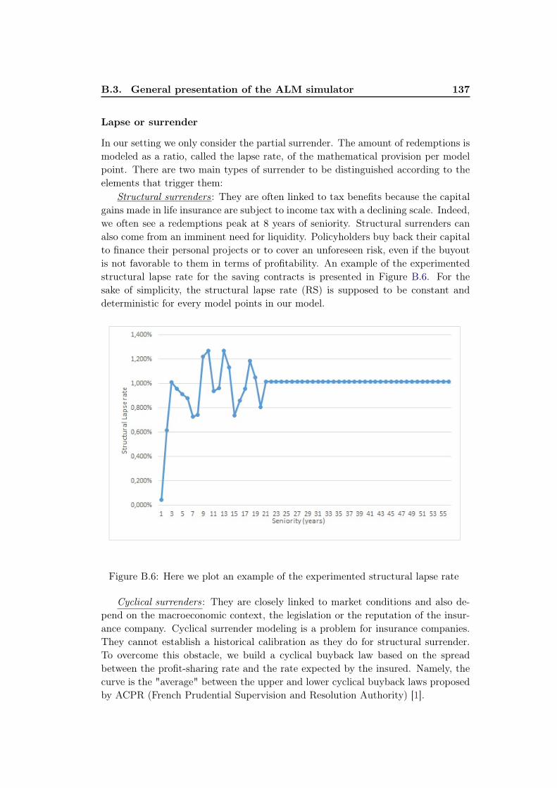
B.3. General presentation of the ALM simulator 137
Lapse or surrender
In our setting we only consider the partial surrender. The amount of redemptions ismodeled as a ratio, called the lapse rate, of the mathematical provision per modelpoint. There are two main types of surrender to be distinguished according to theelements that trigger them:
Structural surrenders: They are often linked to tax benefits because the capitalgains made in life insurance are subject to income tax with a declining scale. Indeed,we often see a redemptions peak at 8 years of seniority. Structural surrenders canalso come from an imminent need for liquidity. Policyholders buy back their capitalto finance their personal projects or to cover an unforeseen risk, even if the buyoutis not favorable to them in terms of profitability. An example of the experimentedstructural lapse rate for the saving contracts is presented in Figure B.6. For thesake of simplicity, the structural lapse rate (RS) is supposed to be constant anddeterministic for every model points in our model.
Figure B.6: Here we plot an example of the experimented structural lapse rate
Cyclical surrenders: They are closely linked to market conditions and also de-pend on the macroeconomic context, the legislation or the reputation of the insur-ance company. Cyclical surrender modeling is a problem for insurance companies.They cannot establish a historical calibration as they do for structural surrender.To overcome this obstacle, we build a cyclical buyback law based on the spreadbetween the profit-sharing rate and the rate expected by the insured. Namely, thecurve is the "average" between the upper and lower cyclical buyback laws proposedby ACPR (French Prudential Supervision and Resolution Authority) [1].
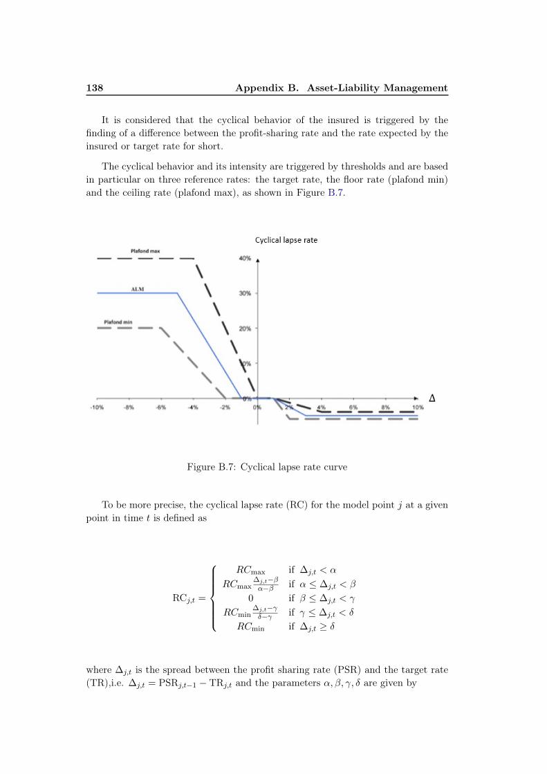
138 Appendix B. Asset-Liability Management
It is considered that the cyclical behavior of the insured is triggered by thefinding of a difference between the profit-sharing rate and the rate expected by theinsured or target rate for short.
The cyclical behavior and its intensity are triggered by thresholds and are basedin particular on three reference rates: the target rate, the floor rate (plafond min)and the ceiling rate (plafond max), as shown in Figure B.7.
Figure B.7: Cyclical lapse rate curve
To be more precise, the cyclical lapse rate (RC) for the model point j at a givenpoint in time t is defined as
RCj,t =
RCmax if ∆j,t < α
RCmax∆j,t−βα−β if α ≤ ∆j,t < β
0 if β ≤ ∆j,t < γ
RCmin∆j,t−γδ−γ if γ ≤ ∆j,t < δ
RCmin if ∆j,t ≥ δ
where ∆j,t is the spread between the profit sharing rate (PSR) and the target rate(TR),i.e. ∆j,t = PSRj,t−1 − TRj,t and the parameters α, β, γ, δ are given by

B.3. General presentation of the ALM simulator 139
Parameter Plafond min Plafond max ALM
α -6% -4% -5%β -2% 0% -1%γ 1% 1% 1%δ 2% 4% 3%
RCmin -6% -4% -5%RCmax 20% 40% 30%
This redemption law is divided into three zones reflecting three behaviors ofpolicyholders according to the difference between the profit-sharing rate and theexpected rate:
• Unfavorable situation: the profit-sharing rate is below the target rate, i.e.∆ < 0, which is below the insured’s expectations. Positive cyclical surrendersare triggered.
• Favorable situation: the profit-sharing rate is included in the [TR+β,TR+γ]
interval, which is close to the rate expected by the insured. Cyclical surrendersare void.
• Very favorable situation: The profit-sharing rate is beyond the target rate, i.e.∆ > 0, which is beyond the expectations of the insured. Cyclical surrendersare negative and offset all or part of the structural buybacks.
Finally, the lapse rate (LR) is calculated as the sum of the structural lapse rateand the cyclical lapse rate as follows:
LRj,t = min (1,max (0, RS +RCj,t)) (B.7)
B.3.3 Chronology of the Asset-Liability interactions
In the framework of the calculation of the BEL, the ALM model makes it possible toproject over a given time horizon the assets and the liabilities of the balance sheet.It allows to determine at each time step the balance sheet and the value of the cashflows distributed to the policyholders on the one hand and to the shareholders onthe other hand.
During each projection period, the following operations are performed:
• Liability cash flows: The insurer collects the premiums and pays the benefitsrelating to the contracts taken out by the insureds. In practice, the liabilitiescash flows are collected and paid throughout the year. In order to facilitatethe calculation of cash flows, we assume that the liabilities cash flows occurmid-period within the stochastic projection model. The modeling of liabilityflows within the stochastic projection model is presented in Section (B.3.2).
• Financial production: The insurer receives the returns from the assets held inthe portfolio.

140 Appendix B. Asset-Liability Management
The interactions between assets and liabilities occur at the end of each period overthe duration of the stochastic projection. These interactions are as follows:
• Purchase and sale of assets: Invest the premiums collected during the period(purchase of assets); finance the claims paid during the period (sale of assets).
• Profit-sharing strategy : profit-sharing rates are calculated for contracts eli-gible for profit-sharing which takes into account regulatory and contractualconstraints. The profit-sharing strategy is described in Section B.3.4.
• Calculation of liabilities at the end of the period : the contracts are revaluedvia the corresponding profit-sharing rates calculated previously. The explicitcalculation of the liabilities at the end of the period is presented in Section [?].
Note that at the end of the projection (after the profit-sharing strategy), theresidual general reserves deemed to belong to the insurer are included in theprofit, those deemed to belong to the insured are included in the BEL.
• Assets reallocation: In accordance with the target asset allocation, the insurerwill buy or sell assets to meet the predefined target asset allocation at the endof the period.
The modeled general reserves (capitalization reserve (RC), provision for risk onthe equity portfolios (PRE) and profit-sharing provision (PPE)) are recalculatedfollowing the purchases and sales of assets.
The following illustration (Fig. B.8) shows the chronology of operations per-formed during a projection period.
Figure B.8: Chronology of the Asset-Liability interactions
B.3.4 Profit-sharing strategy
The profit-sharing strategy is a central element of the ALM model. On the one hand,it plays a role of leverage in the business development of the insurance company,
B.3. General presentation of the ALM simulator 141
because it has an impact on the satisfaction level of policyholders, and on the otherhand, it is subject to regulatory constraints aimed at protecting the interest of theinsured.
In the following, we will give the details of this profit-sharing strategy.
Calculation of Profit-sharing rate
The insurer must at least serve the guaranteed minimum rate (TMG) as defined inthe contract with its insureds. This amount can only be financed by the financialresults of the company. In case of insufficient incomes, the insurer will draw on itsown funds and will realize a loss.
In any case, the insurer cannot use the PPE from previous years to serve theTMG. But once the wealth acquired in this year makes it possible to serve theTMG, the insurer has the right to take over the PPE to provide policyholders abetter revaluation rate. More specifically, the insurer will serve the insureds a so-called net desired rate (NDR), which is defined by
NDRj,t = max (TRj,t − RSj ;TMGj) (B.8)
where RSj is the rate sensibility for the model point j mentioned in Section B.3.2.But what is exactly the meaning of the rate sensibility? In fact, the target ratecorresponds to the desired rate on products subject to strong commercial pressure(flagship products). On less exposed (non-flagship) contracts, the policyholder willbe less sensitive and the expected rate may be reduced by a spread. This latter isset according to the policyholder’s sensitivity to its profit-sharing rate. This is whythe spread is called the rate sensitivity. For the flagship products, this spread is setto 0.
For the latter use, we define the gross desired rate (GDR) and the gross TMG(GTMG) for the model point j as
GDRj,t = NDRj,t + MRj (B.9)
andGTMGj = TMGj + MRj (B.10)
where MRj is the margin rate mentioned in Section (B.3.2).Now the question is what profit-sharing rate the insurer will be able to serve.
To this end we define at first different notions of wealth.First, we define the targets that the insurer seeks to achieve: the "TMG wealth"
and the "desired wealth". They are obtained with a capitalization of the mathe-matical provisions with respectively the TMG and the net desired rate. Namely, wehave
WealthTMGj,t = PMj,t−1(1 + GTMGj) + (Pj,t − Clj,t)
√1 + GTMGj
− (PMj,t−1 + Pj,t − Clj,t)
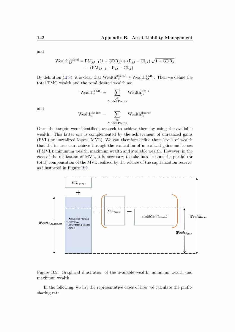
142 Appendix B. Asset-Liability Management
and
Wealthdesiredj,t = PMj,t−1(1 + GDRj) + (Pj,t − Clj,t)
√1 + GDRj
− (PMj,t−1 + Pj,t − Clj,t)
By definition (B.8), it is clear that Wealthdesiredj,t ≥WealthTMG
j,t . Then we define thetotal TMG wealth and the total desired wealth as:
WealthTMGt =
∑j∈
Model Points
WealthTMGj,t
andWealthdesired
t =∑j∈
Model Points
Wealthdesiredj,t
Once the targets were identified, we seek to achieve them by using the availablewealth. This latter one is complemented by the achievement of unrealized gains(PVL) or unrealized losses (MVL). We can therefore define three levels of wealththat the insurer can achieve through the realization of unrealized gains and losses(PMVL): minumum wealth, maximum wealth and available wealth. However, in thecase of the realization of MVL, it is necessary to take into account the partial (ortotal) compensation of the MVL realized by the release of the capitalization reserve,as illustrated in Figure B.9.
Figure B.9: Graphical illustration of the available wealth, minimum wealth andmaximum wealth.
In the following, we list the representative cases of how we calculate the profit-sharing rate.

B.3. General presentation of the ALM simulator 143
Case 1 : WealthTMGt ≥Wealthmax
t :In this case the insurer has to first draw on its own funds a certain amount in
order to serve the TMG and then use the PPE to reach a) the desired rate or b) thecorresponding maximum profit-sharing rate that we can serve (see Figure B.10).
Figure B.10: Case 1: WealthTMGt ≥Wealthmax
t
Case 2 : Wealthavailablet ≤ WealthTMG
t ≤ Wealthmaxt and Wealthdesired
t ≤Wealthmax
t + PPEt−1:The insurer must first realize a portion of unrealized gains to serve the TMG
before the resumption of the PPE to serve the desired rate. (see Figure B.11). Moreprecisely, the unrealized gains needed to be realized is given by
PVREquity = minmax(WealthTMGt −Wealthavailable
t ;
Wealthdesiredt −Wealthavailable
t − PPEt−1);
PVLEquity.
Case 3 : Wealthmint ≤ WealthTMG
t ≤ Wealthavailablet and Wealthdesired
t ≤Wealthavailable
t + PPEt−1:The insurer is able to serve the TMG and the desired rate with the available
wealth. Moreover, we can realize in this case a portion of unrealized loss (see Figure

144 Appendix B. Asset-Liability Management
Figure B.11: Case 2: Wealthavailablet ≤WealthTMG
t ≤Wealthmaxt andWealthdesired
t ≤Wealthmax
t + PPEt−1
B.12). In the same way as previously, the realized loss is determined by comparingdifferent levels of wealth
MVR = minWealthavailablet −WealthTMG
t ;
Wealthavailablet + PPEt−1 −Wealthdesired
t ;
MVLrealizable.
Figure B.12: Case 3: Wealthmint ≤WealthTMG
t ≤Wealthavailablet and Wealthdesired
t ≤Wealthavailable
t + PPEt−1
.
Case 4 : WealthTMGt ≤Wealthmax
t and Wealthmaxt + PPEt−1 <Wealthdesired
t :The insurer can not serve the desired rate despite the realization of all its un-
realized gains. We will therefore serve a profit-sharing rate corresponding to its

B.3. General presentation of the ALM simulator 145
maximum level of wealth (see Figure B.13).
Figure B.13: Case 4: WealthTMGt ≤ Wealthmax
t and Wealthmaxt + PPEt−1 <
Wealthdesiredt
.
Case 5 : Wealthdesiredt ≤Wealthmin
t :In the best case, the insurer can not only serve the desired rate but only make
a profit (see Figure B.14).
Figure B.14: Case 5: Wealthdesiredt ≤Wealthmin
t
.
In regulation, insurance companies must redistribute at least 85% of the financialproducts (if any) to the insureds. It is therefore necessary to verify at the end of

146 Appendix B. Asset-Liability Management
the wealth distribution process that this regulatory condition is well verified. Inpractice, we will cap the margin to be distributed to shareholders at 15% of allfinancial income by putting the surplus in the PPE.
B.3.5 End-of-period liabilities modeling
Own funds
In practice, during the projection of the activity of the insurance companies, theprofits are never redistributed to the shareholders. Therefore, we assume that thefinal own funds BOFt, in our model, becomes the previous own funds BOFt−1 towhich all the results Rt are added. This assumption then makes it possible tocalculate the own funds at the end of each year as follows
BOFt = BOFt−1 + Rt.
B.4 ALM modeling consistency - Leakage test
In order to verify that the ALM model is consistent and correctly implemented,we verify that there is no value leakage during projections. This test is called theleakage test. It consists of comparing the market value of liabilities with the marketvalue of assets at t = 0. Namely, we have to ensure that the following equationholds BELt=0 + VIFt=0 = Assetst=0, where VIFt=0 stands for the value-of-in-forcebusiness at t = 0. Recall that the value-of-in-force business (VIF) is a concept usedwithin insurance that essentially refers to the future profits expected to emerge froma particular life insurance portfolio. Mathematically, it is defined as
VIFt=0 = EQ
[T∑t=1
DF (0, t) (Φt + Pt − Clt −∆PMt −∆PPEt −∆RCt −∆PREt)
]where
• Clt the policyholder claims occured over the period of t to t+ 1,
• Pt the periodic primes paid by the policyholders over the period of t to t+ 1,
• Φt the financial result between the time t and t+ 1.
To better understand the leakage test, a derivation of the previous equa-tion in case of a deterministic projection is given in the following. Bydefinition, we have BELt=0 =
∑Tt=1 P (0, t) (Clt − Pt) and VIFt=0 =∑T
t=1 P (0, t) (Φt + Pt − Clt −∆PMt −∆PPEt −∆RCt −∆PREt). Therefore,
BELt=0 + VIFt=0 =
T∑t=1
P (0, t) (Φt −∆PMt −∆PPEt −∆RCt −∆PREt) .
For later use, let us denote by

B.4. ALM modeling consistency - Leakage test 147
• Casht the cash return on capital deposited on saving account,
• Divt the dividend paid to shareholders,
• Cpnt the coupon collected on the investment bonds,
• Amortizationt the carrying value of a bond portfolio,
• PMVRbondst ,PMVReqt the realized capital gains and losses arising from finan-cial operations on bonds and equities respectively.
The financial result Φt includes the dividend Divt, the cash return Casht, the couponCpnt, the carrying value Amortizationt and the realized capital gains and lossesPMVRt, i.e.
Φt = Divt + Casht + Cpnt + Amortizationt + PMVRbondst + PMVReqt .
We denote by MVt+ ,MVt− the market values of a financial product at the beginningand at the end of the year t, and by α, β the allocations (in percentage) of equitiesand bonds. It is not difficult to note that
Divt = qMVeq(t−1)−
Casht = R(t− 1, t) [(1− α− β)PMt−1 + PPEt−1 + RCt−1 + PREt−1]
PMVReqt = α (PMt − PMt−1) +(MVeq
t+−MVeq
t−
)= α (PMt − PMt−1) + (1 +R(t− 1, t)− q)MVeq
(t−1)− −MVeqt−
Amortizationt + PMVRbondst = β (PMt − PMt−1) +(MVbondst+ −MVbondst−
)and
MVbondst− = P (t− 1, t)(MVbonds(t+1)+ + Cpnt+1
)=P (0, t+ 1)
P (0, t)
(MVbonds(t+1)+ + Cpnt+1
)Combining all these equations together, we get finally
P (0, t)(Φt −∆PMt −∆PPEt −∆RCt −∆PREt)
= P (0, t− 1)[MVeq(t−1)− + MVbonds(t−1)− + (1− α− β)PMt−1
+ PREt−1 + RCt−1 + PPEt−1]− P (0, t)[MVeqt− + MVbondst−
+ (1− α− β)PMt + PREt + RCt + PPEt] (B.11)
Since we liquidate all the liabilities at the end of projection, we have to addP (0, T )[MVeq
T− +MVbondsT− + (1−α− β)PMT +PRET +RCT +PPET ] on the right-hand side of the equation (B.11) at t = T . With a little bit of algebra, it is easy toshow that
BELt=0 + VIFt=0 = MVeq0 + MVbonds0 + (1− α− β)PM0 + PRE0 + RC0 + PPE0
= Assett=0.

148 Appendix B. Asset-Liability Management
Figure B.15: Comparison of the market value of assets and the market value ofliabilities at t = 0 given the deterministic scenario.
By freezing all the volatility terms to be zero (deterministic scenario), we findthat there is no leakage in our ALM model (see Fig B.15). We also perform theleakage test for the probabilistic simulations. In this case, we will observe the leaksin our simulations mainly explained by the finite numbers of simulations. To thisend, we define the leakage ratio as
Lε =|BELt=0 + VIFt=0 −Assett=0|
Assett=0
We iterate the simulation with 100 different random seeds. For each simulation, wecompute the BEL and the VIF using Monte-Carlo method with NMC number ofsimulations. Then we compute the mean squared error defined by
MSE =1
100
100∑j=1
(L(j)ε
)2
where the index j stands for the jth random state. Finally, we obtain the followingresults
NMC MSE(×10−4)
103 83.2
104 11.5
105 0.98

B.4. ALM modeling consistency - Leakage test 149
In the above table we can see that the leaks are significantly reduced as thenumber of simulations increases.


Appendix C
Demonstration of the θt equation
The Hull White model reproduces exactly the zero-coupon rate curve, if
θt =d
dtf(0, t) + a.f(0, t) +
σ2
2a
(1− e−2at
)(C.1)
Proof. We assume that the zero-coupon price at maturity T is written as a functionof t and the short rate rt. So we have P (t, T ) = h(t, rt). Let’s apply the formula ofItô to h(t, rt), in order to find a partial differential equation verified by h:
dP (t, T ) =
(dh
dt+dh
drt(θt − art) +
1
2
d2h
dr2t
σ2
)dt+
dh
drtσdWt
However, under the neutral risk probability, dP (t, rt) = rtP (t, rt)dt since the zero-coupon bond is considered as the risk-free asset. By uniqueness, we obtain thefollowing partial differential equation
dh
dt+dh
drt(θt − art) +
1
2
d2h
dr2t
σ2 = rtP (t, rt) (C.2)
In addition, f(T, rT ) = P (T, T ) = 1 by definition of a zero-coupon bond.We then seek to find a solution of the equation (C.2) of form: f(t, rt) = P (t, T ) =
A(t, T )e−B(t,T )rt . By differentiating P in terms of t and rt, and by simplifying bye−B(t,T )rt :
dA(t,T )dt − θtA(t, T )B(t, T ) + 1
2σ2A(t, T )B2(t, T ) = 0
1 + dB(t,T )dt − aB(t, T ) = 0
with A(T, T ) = 1 and B(T, T ) = 0.We then obtain
B(t, T ) =1
a
(1− e−a(T−t)
)and
lnA(t, T ) = −∫ T
tθuB(u, T )du− σ2
2a(B(t, T )− (T − t))− σ2
4aB2(t, T )
With the expression of A and B, we have the zero coupon price expression in theHull & White model, we can infer an expression of today’s instantaneous forwardrates for all maturities T
f(0, T ) =
∫ T
0θudB(u, T )
dTdu+
dB(0, T )
dTr0 −
σ2
2aB(0, T )
(1− dB(0, T )
dT
)

152 Appendix C. Demonstration of the θt equation
Let us differentiate the above equation by T , we have
df(0, T )
dT= θT − af(0, T )− σ2
2a
(1− e−2aT
)

Appendix D
Bayesian P-spline regression andBayesian asymptotic confidence
interval
In this section, a brief description of smoothing and penalized splines (or P-splines)will be presented. Some interesting additional information about smoothing splinesand P-splines can be found for example in the work of Reinsch [94], Duchon [31],Green and Silverman [43], Hastie and Tibshirani [49], Eubank [35], Eilers and Marx[32] and Ruppert and Carroll [96].
Consider the regression model Yi = m(Xi) + εi, i = 1, . . . , n where εi are theindependent random variables with mean 0 and variance σ2. We assume that thedesign points Xi ∈ [a, b] with a, b < ∞. As pointed out in Appendix (D.7), forany regular functions m(x), we can always find a best spline approximation m(x) ofm(x) to minimize ‖m− m‖∞. The error in approximating m(x) by m(x) is usuallynegligible compared to the estimator error, thus in practice we estimate m(x) insteadof m(x). In the following, we denote by B(x) = B1(x), . . . , BN (x)T ∈ RN , N ≤ na spline basis.
D.1 Smoothing Splines
The key idea of this regression method is to approximate the target function m(x)
by a natural cubic spline m(x) with knots at the distinct Xi values. The basisfunctions for natural cubic splines are
1, x, d1(x)− dn−1(x), . . . , dn−2(x)− dn−1(x)
where dk(x) =(x−Xk)3
+−(x−Xn)3+
Xn−Xk for k = 1, . . . , n− 1.A smoothing spline estimator arises as the minimizer of the penalized sum of
squares,n∑i=1
(Yi − m(Xi))2 + λ
∫ b
a
(m”(x)
)2dx (D.1)
for λ > 0.The integral term in the previous expression is a roughness penalty with the
smoothing parameter λ. We write the vector m = (m(X1), . . . , m(Xn))T ∈ Rn.The theorem 2.1 in Green and Silverman [43] shows that there exists a n × n

154Appendix D. Bayesian P-spline regression and Bayesian asymptotic
confidence interval
dimensional matrix K of rank n − 2 such that the penalty term∫ ba
(m”(x)
)2dx
can be written as mTKm. The smoothing spline estimate at the design pointsm = (m(X1), . . . , m(Xn))T ∈ Rn is thus explicitly given by m = (I + λK)−1 Y
where Y = (Y1, . . . , Yn)T ∈ Rn. This regression method is however less practicalwhen the number of design points n becomes large since it uses n knots.
D.2 Regression Penalized Splines or P-Splines
The idea of penalized spline smoothing with basic functions can track back toO’Sullivan [87], see also Eilers and Marx [32] and Ruppert and Carroll [96] foradditional information. Two common basis used in practical, up to our knowledges,are the B-spline basis (Eilers and Marx [32], De Boor [25]) and the truncated powerbasis (Ruppert and Carroll [96]). The B-spline basis is preferable for computationbecause of its better numerical properties. For formulation and theoretical studythe truncated power basis is preponderant because of its simplicity.
The penalized spline model specifies that the estimate m(x) is expressed asB(x)Tβ for some N -dimensional space. Hence, the estimation of m(x) is equivalentto that of β. Let D be a fixed, symmetric, positive semidefinite N × N matrix,which is equivalent to the matrix K in the smoothing spline model. The penalizedspline estimator β arises as the minimizer of
n∑i=1
(Yi −B(Xi)β)2 + λβTDβ (D.2)
Define B the n × N matrix whose i-th row equals B(Xi)T . The penalized spline
estimator is thus written as β = (BTB + λD)−1BTY . From this, we obtain:
E(β)
=(BTB + λD
)−1BTBβ (D.3)
and the covariance of the estimate
Vβ = σ2(BTB + λD
)−1BTB
(BTB + λD
)−1 (D.4)
It follows that β ∼ N(E(β),Vβ
). It is clear that E
(β)6= β except for β = 0
which leads to the difficulty in using this result for calculating confidence intervals.In this paper, we choose the truncated p-polynomial basis as mentioned previ-
ously, i.e. B(x) =(1, x, x2, . . . , xp, (x− κ1)p+, . . . , (x− κK)p+
)T for p ≥ 1 and D
is the diagonal matrix diag(0p+1,1K), indicating that only the spline coefficientsare penalized. One can easily verify that
∫ ba
[m(p+1)(x)
]2dx = (p!)2
∑Kj=1 β
2j+p by
using the fact that the derivative of an indicator function is a Dirac delta function.Therefore, the equation (D.2) can be rewritten as
n∑i=1
(Yi − m(x))2 + λ′∫ b
a
[m(p+1)(x)
]2dx (D.5)
which is a generalization of equation (D.1).
D.3. Bayesian Analysis for Penalized Splines Regression 155
D.3 Bayesian Analysis for Penalized Splines Regression
The Bayesian analysis for penalized spline regression is an alternative approach tocalculate the confidence intervals. The initial works for this approach is mainlydue to Wahba [115] and Silverman [99]. The main idea behind this method is topartition the coefficient vector β into the coefficients of the monomial basis func-tions of the truncated power functions by letting β = (βT1 , β
22)T where β1 ∈ R1+p
has an improper uniform prior density and β2 ∈ RK has a proper prior equal to(λ/σ2)K/2 exp
(−(λ/2σ2)βT2 β2
).
Following the idea of Wood (section 4.8.1 in [119]), we obtain the Bayesianposterior covariance matrix for the parameter β:
Vβ =(BTB + λD
)−1σ2 (D.6)
and its corresponding posterior distribution:
β|Y ∼ N(β,Vβ
)(D.7)
where β = (BTB + λD)−1BTY . The penalized least squares estimator is themean of the posterior distribution of β. This posterior on β induces a posterioron m(·) and then the posterior distribution of m = (m(X1), . . . , m(Xn))T , i.e.m|Y ∼ N (AY, σ2A) with A = B(BTB + λD)−1BT .
D.4 Bayesian Asymptotic Confidence Interval
Nychka [84] showed that if m(x) is estimated using a cubic smoothing spline forwhich the smoothing parameter is sufficiently reliably estimated that the bias in theestimates is a modest fraction of the mean squared error for m(x), then the averagecoverage probability (ACP)
ACP =1
n
n∑i=1
P (m(Xi) ∈ BIα(Xi))
is very close to the nominal level 1 − α, where BIα(x) indicates the (1 − α)100%
Bayesian interval for m(x) and α the significance level. This is due to the fact thatthe average posterior variance for the spline is similar to a consistent estimate ofthe average squared error and that the average squared bias is relatively small withrespect to the total average squared error.
Marra and Wood [80] modified Nychka’s [84] approach to obtain the confidenceinterval for Generalized Additive Model (GAM ), which is also applicable in theBayesian penalized spline models. Here we will sketch the main steps to obtainconfidence interval of variable width.
Given some constants Ci, which will be defined later, the primary purpose is tofind a constant A, such that
ACP =1
n
n∑i=1
P(|m(Xi)− m(Xi)| ≤ zα/2A/
√Ci
)= 1− α (D.8)

156Appendix D. Bayesian P-spline regression and Bayesian asymptotic
confidence interval
where zα/2 is the α/2 critical point from a standard normal distribution.Letting m = (m(X1), . . . , m(Xn))T = Bβ and m = (m(X1), . . . , m(Xn))T =
Bβ. We write the covariance of m as Vm = BVβBT and the same as that
of m, i.e. Vm = BVβBT . Define b ≡ (b(X1), . . . , b(Xn))T = E(m) − m and
v ≡ (v(X1), . . . , v(Xn))T = m − E(m). We have v ∼ N (0,Vm) following frommultivariate normality of m. Equivalently, the equation (D.8) can be written as:
ACP = P(|b(XI) + v(XI)| ≤ zα/2A/
√CI
)= P
(|B + V| ≤ zα/2A
)= 1− α (D.9)
where I is a random variable uniformly distributed on 1, 2, . . . , n, B and V arerespectively the random scaled bias and random scaled variance defined as follows:
B =√CIb(XI) and V =
√CIv(XI).
This means that we need to know the distribution of B + V in order to find theconstant A.
Clearly, by definition, we have E(B) = cTB (Fβ − β), E(V) = 0 and var(V) =
tr(CVm)/n where c =(√C1, . . . ,
√Cn)T , F = (BTB + λB)−1BTB and C is the
diagonal matrix diag (C1, . . . , Cn). Since v ∼ N (0,Vm), V is a mixture of normals.However, if we choose C−1
i = [Vm]ii, the random scaled variance V then has anormal distribution. Since its distribution no longer depends on i, it implies theindependence of B and V.
We call M the scaled average mean squared error which is given by:
M =1
n
n∑i=1
Ci (m(Xi)− m(Xi))2 . (D.10)
The mean squared error E (M) can be then determined as follows:
E(M) =1
nTr(BTC2BVβ
)+
1
n‖CB (F− I)β‖2. (D.11)
By construction, we have E(B + V) = E(B) and var(B + V) = E(M) − E(B)2.Nychka’s [84] simulation results showed that B+V will be approximately normallydistributed, provided that B is small relative to V, i.e.
B + V ∼ N(E(B),E(M)− E(B)2
)The expectations E(B) and E(M) can be estimated by substituting β by β whichyields
E(B) = cTB(Fβ − β)/n
and
E (M) =1
nTr(BTC2BVβ
)+
1
n‖CB (F− I) β‖2
= 1 +1
n‖CB (F− I) β‖2 (D.12)

D.5. Additive model and Asymptotic confidence interval for eachfunctional components 157
Therefore, we have the approximate result
B + V ∼ N(E(B), E(M)− E(B)
2)
under the assumption that B is small relative to V, i.e. b2 v2.
As the definition (D.9), it follows that A =
√E(M)− E(B)
2and then we obtain
m(Xi)− E(B)√
[Vm]ii ± zα/2
√(E(M)− E(B)
2)
[Vm]ii (D.13)
as the definition of 1− α Bayesian asymptotic confidence intervals at the point Xi.Finally, we use the estimator σ2 = ‖Y−Bβ‖2
n−Tr(F) to estimate σ2.
D.5 Additive model and Asymptotic confidence intervalfor each functional components
In this section, the additive model will be briefly presented. In this model therelation between the response Yi, i ∈ 1, . . . , n and the d-explanatory variablesX1i, X2i, . . . , Xdi is expressed through arbitrary univariate functions fj as follows:
Yi = β0 +
d∑j=1
fj (Xji) + εi (D.14)
where the errors εi are independent and identically distributed with mean zeroand the variance σ2. Several estimation strategies have been developed to fit sucha model, e.g. backfitting algorithm (Hastie and Tibshirani [49]) as well as itsasymptotic statistical properties (Opsomer and Ruppert [85], Opsomer [86] andWand [116]), and a marginal integration approach (Linton and Nielsen [77]). Dueto the computational expediency, the penalized splines regression to ordinary ad-ditive models (Hastie and Tibshirani [49]) have been widely used in practice. Asconsequent, we will apply this approach to estimate the excess loss function.
Like the univariate case, each of the functional components fj is modeledas BTβj a degree pj penalized spline estimator with smoothing parameters λjand Bj a n × (pj + Kj) matrix whose i-th row is (Xji, X
2ji, . . . , X
pjji , (Xji −
κj1)pj+ , . . . , (Xji − κjKj )
pj+ ). However, for the identifiability reasons, we replace
fj(·) by fj(·) − 1/n∑n
i=1 fj(Xji) which leads to the condition on fj(·) of the form∑ni=1 fj(Xji) = 0. Therefore, the estimate of β0 is β0 = Y ≡ 1
n
∑ni=1 Yi which is
independent of Xji’s and the matrix Bj is adjusted to B∗j = 1n(I − 1.1T )Bj where
I is the identity matrix and 1 is a n× 1 column of ones. This adjustment is calledthe “centering effect”. Letting Y ∗ = (Y1 − β0, . . . , Yn − β0)T , B = [B∗1, . . . ,B
∗d]
and Dλ = blockdiag1≤j≤d(λjDj) with λj > 0. We then have the estimate ofβT = (βT1 , . . . , β
Td ) is given by
β =(BT B + Dλ
)−1BY ∗ ∈ R
∑dj=1(pj+Kj+1) (D.15)
158Appendix D. Bayesian P-spline regression and Bayesian asymptotic
confidence interval
From this we derive the estimate of βj , βj = Pj β where Pj =
[0, . . . ,1(pj+Kj+1), . . . , 0] ∈ R(pj+Kj+1)×∑k(pk+Kk+1).
Regarding the Bayesian asymptotic confidence interval for each of the functionalcomponents, the derivation is analogue as for the univariate case. Namely, assumethat β0 has an improper uniform prior distribution and the prior for βj is given by(λj/σ
2)Kj/2 exp(−(λj/2σ
2)βTj βj
)for j = 1, . . . , d. By using Bayes rule, it has been
shown ( [119]) thatβ|Y ∼ N
(β,Vβ
)where Vβ = (BT B + Dλ)−1σ2. Thanks to the equation (D.15), it is then routine toshow that Vβ = (BT B + Dλ)−1BT B(BT B + Dλ)−1σ2. It follows immediately thatthe variance of fj is Vfj
= (B∗jPj)Vβ(B∗jPj)T . The 1 − α Bayesian asymptotic
confidence interval computation for fj(Xji) is similar to that can be found in (D.4).Routine manipulation then results in
fj (Xji)− E(Bj)
√[Vfj
]ii± zα/2
√(E(Mj)− E(Bj)
2)[
Vfj
]ii
(D.16)
as the definition of 1−α Bayesian asymptotic confidence interval for fj(Xji). Here,we denoted E(Bj) = 1
ncTB∗jPj
(Fβ − β
)with c =
([Vfj
]−1/211 , . . . , [Vfj
]−1/2nn
)and F = (BT B + Dλ)−1BT B, E(Mj) = 1 + 1
n‖CjB∗jPj(Fβ − β)‖ with Cj =
diag([Vfj]−111 , . . . , [Vfj
]−1nn). Readers can refer to [80] for more details.
D.6 Upper bound of the probabilities of deviation
1. Let us denote Sj = |φj(x
(ν)j
)− φj
(x
(ν)j
)| > ∆
(ν)j,α and Sj = |hJ
(x
(ν)J
)−
hJ
(x
(ν)J
)| > ∆
(ν)J,α. Since Sj and SJ are mutually independent, it implies that
(by De Morgan’s law)
P
⋃j
Sj
⋃(⋃J
SJ
) = 1− P
⋂j
Scj
⋂(⋂J
ScJ
)= 1−
∏j
P(Scj )
×(∏J
P(Scj )
)
which asymptotically tends to 1− (1−α)d(d+3)/2 as Γ→∞. With this the equation(3.28) is then a straightforward consequence of the relation
P
|φ(x(ν))− φ(x(ν))| >d∑j=1
∆(ν)j,α +
∑J
∆(ν)J,α
≤ P
⋃j
Sj
⋃(⋃J
SJ
)thanks to the equation (3.27).

D.7. Best approximation by splines 159
2. For a given value of Γ, we call r∗ ≡ r(Γ) the positive constant mentioned inAssumption (3). Furthermore, we assume that B(x∗, r∗) ⊂ Ω for large enough Γ.
For notional simplicity, let us denote δφ(x, y) = |φ(y)− φ(x)|. We have
P(δφ(x∗, x∗(Γ)) > ∆(α,Γ) + Lr∗
)= P
(δφ(x∗, x∗(Γ)) > ∆(α,Γ) + Lr∗ | x∗(Γ) ∈ B(x∗, r∗)
)P(x∗(Γ) ∈ B(x∗, r∗)
)+ P
(|φ(x∗(Γ))− φ(x∗)| > ∆(α,Γ) + Lr∗ | x∗(Γ) /∈ B(x∗, r∗)
)P(x∗(Γ) /∈ B(x∗, r∗)
)≤ P
(δφ(x∗(Γ), x
∗(Γ)) > ∆(α,L) | x∗(Γ) ∈ B(x∗, r∗)
)+ ξ(r∗, d)Γ−γ(r∗,d)
since |φ(x∗(Γ))− φ(x∗)| ≤ |φ(x∗(Γ))− φ(x∗(Γ))|+ |φ(x∗(Γ))− φ(x∗)| and
P(|φ(x∗(Γ))− φ(x∗)| > Lr∗ | x∗(Γ) ∈ B(x∗, r∗)
)= 0
thanks to Assumption (1).Finally, by applying Assumption (3), we obtain
P(δφ(x∗, x∗(Γ)) > ∆(α,Γ) + Lr∗
)≤[1− (1− α)d(d+3)/2
]+ ξ(r∗, d)Γ−γ(r∗,d).
D.7 Best approximation by splines
Let us first introduce two functional spaces.
Definition 3 (Polynomial Spline Space Φa,bs ). Letting κl for l ∈ 1, . . . ,K be K-
interior knots satisfying the condition a = κ0 ≤ κ1 ≤ · · · ≤ κK ≤ κK+1 = b. Wedefine Φa,b
s the space of functions whose element is a polynomial of at most degreep on each of the intervals [κl, κl+1) for l = 0, 1, . . . ,K and is p − 1 continuouslydifferentiable on [a, b] if p ≥ 1.
Definition 4 (Empirically Centered Polynomial Spline Space Φa,bs ). Given the de-
sign points (x1, . . . , xn) ∈ [a, b]n, a polynomial spline space is centered if for everyg ∈ Φa,b
s the following identity holds:
1
n
n∑i=1
g(xi) = 0.
We denote by Φa,bs the Empirically centered polynomial spline space.
According to de Boor (p.149 in [25]), for every φ(x) ∈ Cp+1([a, b]), there existsa constant c > 0 and a spline function φ∗(x) ∈ Φa,b
s , such that ‖φ − φ∗‖∞ ≤c‖φ(p+1)‖∞δp+1 with δ = max1≤l≤K(κl+1 − κl).
Given the design points (x1, . . . , xn) ∈ [a, b]n, we assume furthermore that
1
n
n∑i=1
φ(xi) = 0
.By defining φ∗∗(x) = φ∗(x)− 1
n
∑ni=1 φ
∗(xi) ∈ Φa,bs , it is straightforward to show
that there exists a positive constant c′ such that ‖φ− φ∗∗‖∞ ≤ c′‖φ(p+1)‖∞δp+1.

160Appendix D. Bayesian P-spline regression and Bayesian asymptotic
confidence interval
D.8 Asymptotic distribution of empirical quantiles
Theorem 5. Let X1, . . . , Xn be n-real valued observations with unknown distribu-tion function F , p be a real number defined in the interval [0, 1], xp = xp(F ) be thepth-percentile of F and Fn(x) be the empirical distribution function.
If we suppose that F is continuous and differentiable at xp of derivation f(xp),then
√n (xp(n)− xp)→ N
(0,p(1− p)f2(xp)
)(D.17)
as n→∞.
This is a well-known result for the asymptotic convergence of empirical quantiles.We will thus omit the proof here. For any further and detailed information, theinterested reader can refer to [113] (see Section 3.9.21)

Bibliography
[1] ACPR, Préparation à Solvabilité II. Enseignements des annexes techniques vieremises en 2013. (Cited on page 137.)
[2] Aerts, M., Claeskens, G. and Wand, M. P., Some theory for penalized splinegeneralized additive models J. Stat. Plan. Inference, 103, 455−470, 2002. (Citedon pages 22 and 55.)
[3] Anderson, L. B. G. and Piterbarg, V. V., Interest Rate Modeling. Atlantic Fi-nancial Press, Business & Economics, 2010. (Cited on page 109.)
[4] Arthur Greenwood, J., Maciunas Landwehr, J., Matalas, N. C. and Wallis, J. R.,Probability weighted moments: Definition and relation to parameters of severaldistributions expressable in inverse form. Water Resources Research, 15, 1979.(Cited on page 77.)
[5] Arvanitis A., Gregory J., and Laurent J. P., Building Models for Credit Spreads.The Journal of Derivatives, 6 (3) 27−43, 1999. (Cited on page 120.)
[6] Balkema, A. A. and de Haan, L., Residual Life Time at Great Age. Annals ofprobability, 2(5): 792−804, 1974. (Cited on page 74.)
[7] Bauer, D., Bergmann, D. and Reuss, A., Solvency II and Nested Simulations-A Least Square Monte Carlo Approach. Proceedings of the 2010 ICA congress,2009. (Cited on page 11.)
[8] Bauer, D., Reuss, A. and Singer, D., On the Calculation of the Solvency CapitalRequirement based on Nested Simulations. ASTIN Bulletin, 42, 453−499, 2012.(Cited on page 4.)
[9] Beirlant, J. and Goegebeur, Y., Local polynomial maximum likelihood estimationfor Pareto-type distributions. Journal of Multivariate Analysis, 89, 97−119, 2004.(Cited on pages 17, 27, 79, 80, 81, 82, 90 and 91.)
[10] Beirlant, J., Goegebeur, Y., Teugels, J. and Segers, J., Statistics of Extremes:Theory and Applications. John Wiley & Sons, Inc. Published 2004. (Cited onpage 75.)
[11] Belloni, A. and Chernozhukov, V., Least squares after model selection in highdimensional sparse model. Bernoulli, 19(2):521−547, 2013. (Cited on page 89.)
[12] Bellman, R. E., Adaptive Control Processes. Princeton University Press, 1961.(Cited on page 46.)
[13] Bengio, Y. and Grandvalet, Y., No unbiased estimator of the variance of k-foldcross-validation. J Mach Learn Res, 5, 1089−1105, 2004. (Cited on page 62.)

162 Bibliography
[14] Bertsekas, D., Nonlinear programming. Athena Scientific, 1999. (Cited onpages 85 and 98.)
[15] Beutner, E., Pelsser, A. and Schweizer, J., (1993) Theory and validation ofreplicating portfolios in insurance risk management. Available athttp://papers.ssrn.com/sol3/papers.cfm?abstract_id=2557368 Accessed20 June 2018. (Cited on page 13.)
[16] Bingham, N.H, Goldie, C.M. and Teugles, J.L., Regular Variation. CambridgeUniversity Press, 1987. (Cited on page 79.)
[17] Black, F. and Scholes, M.. The Pricing of Options and Corporate Liabilities.Journal of Political Economy. 81(3): 637˘654, 1973. (Cited on page 112.)
[18] de Boor, C., A Practical Guide to Splines, Revised Edition. volume 27, AppliedMathematical Sciences, Springer, New York, 2001. (Cited on pages 45 and 99.)
[19] Brigo, D. and Mercurio, F., Interest Rate Model: Theory and Practice. SpringerScience & Business Media, 2013. (Cited on page 109.)
[20] Buja, A., Hastie, T. J. and Tibshirani, R. J., Linear smoothers and additivemodels. Annals of Statistics, 17: 453−510, 1989. (Cited on page 46.)
[21] Burr, I. W., Cumulative frequency functions. Ann of Math Statist, 13, 215−232,1954. (Cited on page 89.)
[22] Chavez-Demoulin, V., Embrechts, P. and Sardy, S., An extreme value approachfor modeling operational risk losses depending on covariates. J Risk Insur, 2014.(Cited on pages 17 and 80.)
[23] Chernobai, A., Jorion, P. and Yu, F., The determinants of operational riskin u.s. financial institutions. Journal of Financial and Quantitative Analysis,46(8):1683−1725, 2011. (Cited on pages 17 and 79.)
[24] Christopeit, N., Estimating parameters of an extreme value distributionby the method of moments. Journal of Statistical Planning and Inference,41(2):173−186, 1994. (Cited on page 77.)
[25] de Boor, C., A Practical Guide to Splines, revised ed. Springer, New York,2001. (Cited on pages 154 and 159.)
[26] de Haan, L. and Rotzen, H., On the estimation of high quantiles. J Stat PlanInference, 35(1), 1−13, 1993. (Cited on page 80.)
[27] de Haan, L. and Ferreira, A. F., Extreme Value Theory - An Introduction.Springer Series in Operations Research and Financial Engineering, 2006. (Citedon pages 72 and 81.)

Bibliography 163
[28] Dekkers, A. L. M., Einmahl, J. H. J. and de Hann, J., A moment estimator forthe index of an extreme-value distribution. Annals of Statistics, 17:1833−1855,1989. (Cited on page 77.)
[29] Dekking, F.M., Kraaikamp, C., Lopuhaä, H.P. and Meester, L.E., A Modern In-troduction to Probability and Statistics: Understanding Why and How. SpringerTexts in Statistics, 2005. (Cited on page 96.)
[30] Devineau, L. and Loisel, S., Construction of an acceleration algorithm of theNested Simulations method for the calculation of the Solvency II economic capi-tal. Bulletin Français d’Actuariat, 2009. (Cited on page 14.)
[31] Duchon, J., Splines minimizing rotation-invariant semi-norms in Sobolevspaces. In Construction Theory of Functions of Several Variables. Springer,Berlin, 1977. (Cited on page 153.)
[32] Eilers, P. H. C. and Marx, B. D., Flexing smoothing with B-splines and Penal-ties. Stat Sci, 11, 89-102, 1996. (Cited on pages 153 and 154.)
[33] EIOPA-14/209, Technical Specification for the Preparatory Phase (Part I), 30April 2014, p.120. (Cited on page 36.)
[34] Embrechts, P., Klüpplberg, C. and Mikosch, T., Modelling Extremal Events.Berlin: Springer, 1997. (Cited on pages 75 and 77.)
[35] Eubank, R. L., Nonparametric Regression and Spline Smoothing. (2nd ed.) Mar-cel Dekker, New York, 1999. (Cited on page 153.)
[36] Filipovic, D., Term-Structure Models: A Graduate Course. Springer FinanceTextbooks, 2009. (Cited on pages 59 and 60.)
[37] Fisher, R. A. and Tippett, L. H. C., Limiting forms of the frequency distributionof the largest or smallest member of a sample. Mathematical Proceedings of theCambridge Philosophical Society, 24(2): 180−190, 1928. (Cited on page 73.)
[38] Friedman, J. H. and Stuetzle, W., Projection pursuit regression. Journal of theAmerican Statistical Association, 76:817−823, 1981. (Cited on page 46.)
[39] Friedman, J., Hastie, T. and Tishirani, R., (2010) A note on the Group Lassoand a Sparse Group Lasso. arXiv:1001.0736.22. (Cited on page 87.)
[40] Giraud, C., Introduction to High-Dimensional Statistics. Chapman and Hall,CRC Monographs on Statistics & Applied Probability, 2014. (Cited on page 62.)
[41] Girsanov, I. V., On transforming a certain class of stochastic processes by ab-solutely continuous substitution of measures. Theory of Probability and its Ap-plications, 5 (3): 285−310, 1960. (Cited on page 114.)
[42] Gnedenko, B., Sur la distribution limite du terme maximum d’une seriealeatoire. Ann Stat, 44(3), 423−453, 1943. (Cited on pages 79 and 80.)

164 Bibliography
[43] Green, P. J. and Silverman, B. W., Nonparametric Regression and GeneralizedLinear Models: A Roughness Penalty Approach. Chapman and Hall, London,1994. (Cited on page 153.)
[44] Gu, C., Multivariate spline regression. In Schimek, M. G., editor: Smoothingand Regression: Approaches, Computation and Applications. Wiley Series inProbability and Mathematical Statistics, 229−356. John Wiley & sons, 2000.(Cited on page 45.)
[45] Gu, C., Smoothing spline ANOVA Models. Springer Series in Statistics,Springer, New York, 2002. (Cited on page 45.)
[46] Hall, P., On some simple estimates of an exponent of regular variation. J RoyStatist Soc Ser B, 44, 37−42, 1982. (Cited on page 89.)
[47] Härdle, W. and Muller, M., Multivariate and semiparametric kernel regression,In Schimek, M. G., editor: Smoothing and Regression: Approaches, Computa-tion and Application. Wiley Series in Probability and Mathematical Statistics,357−392, John Wiley & sons, 2000. (Cited on page 45.)
[48] Hastie, T. and Tibshirani, R., Generalized additive models. Statistical Science,1:297−318, 1986. (Cited on pages 40 and 47.)
[49] Hastie, T. and Tibshirani, R., Generalized Additive Models. volume 43, Mono-graphs on Statistics and Applied Probability, Chapman & Hall, 1990. (Cited onpages 46, 47, 82, 153 and 157.)
[50] Hastie, T. J., Tibshirani, R.J., and Friedman, J., The elements of StatisticalLearning: Data Mining, Inference and Prediction. Springer Series in Statistics,Springer, New York, 2001. (Cited on pages 44 and 46.)
[51] Hawkins, T. Cauchy and the spectral theory of matrices. Historia Mathematica.2:1˘29, 1975. (Cited on page 106.)
[52] Heuchenne, C., Lopez, O. and Hambuckers, J., A semiparametric model forgeneralized pareto regression based on a dimension reduction assumption. Un-publised work, 2014. (Cited on pages 17 and 80.)
[53] Hill, B. M., A simple general approach to inference about the tail of a distribu-tion. Annals of Statistics, 3:1163−1174, 1975 (Cited on page 77.)
[54] Hong, L.J., Juneja, S. and Liu, G., (2017) Kernel smoothing for nested esti-mation with application to portfolio risk measurement. Operations Research, 65,657−673, 2017. (Cited on pages 101 and 102.)
[55] Hosking, J. R. M. and Wallis, J. R., Parameter and quantile estimation forthe generalized Pareto distribution. Technometrics, 29:339−349, 1987. (Cited onpage 78.)

Bibliography 165
[56] Hull, J. and White, A., Pricing interest-rate derivative securities. The Reviewof Financial Studies, 3(4): 573−592, 1990. (Cited on page 108.)
[57] Hull, J. and White, A., One factor interest rate models and the valuation of in-terest rate derivative securities. Journal of Financial and Quantitative Analysis,28(2): 235−254, 1993. (Cited on page 108.)
[58] Hull, J. and White, A., Numerical procedures for implementing term structuremodels I. Journal of Derivatives, 7–16, Fall 1994. (Cited on page 108.)
[59] Hull, J. and White, A., Numerical procedures for implementing term structuremodels I. Journal of Derivatives, 37–48, Winter 1994. (Cited on page 108.)
[60] Hull, J. and White, A., Using Hull–White interest rate trees Journal of Deriva-tives, 3(3), 26˘36, 1996. (Cited on page 108.)
[61] Israel, R. B., Rosenthal, J. S. and Wei, J. Z., Finding generator for Markovchains via empirical transition matrices with application to credit ratings. Math-ematical Finance, 11(2): 245−265, 2001. (Cited on pages 120 and 122.)
[62] Jagannathan, R., Kaplin, A. and Sun, S., An evaluation of multi-factor CIRmodels using LIBOR, swap rates, and cap and swaption prices. Journal of Econo-metrics, 116(1−2):113−146, 2003. (Cited on page 110.)
[63] Jarrow, R. A., Lando, D. and Turnbull, S. M., A Markov Model for the TermStructure of Credit Risk Spreads. The Review of Financial Studies, 10 (2):481−523, 1997. (Cited on page 119.)
[64] Kemp, M., Market Consistency. Wiley Finance, 2009. (Cited on page 33.)
[65] Klinke, S. and Grassmann, J., Projection pursuit regression, In Schimek, M. G.,editor: Smoothing and Regression: Approaches, Computation and Application.Wiley Series in Probability and Mathematical Statistics, 471−496, John Wiley& sons, 2000. (Cited on page 46.)
[66] Koursaris, A., Improving capital approximation using the curve-fitting approach.Barrie & Hibbert (working paper), 2011. (Cited on page 8.)
[67] Koursaris, A., The advantages of least squares Monte Carlo. Barrie & Hibbert.Available athttp://www.barrhibb.com/documents/downloads/The_Advantages_of_Least_Squares_Monte_Carlo.pdf. Accessed 22 June 2018, 2011. (Cited on page 11.)
[68] Koursaris, A., A least squares Monte Carlo approach to liability proxy modellingand capital calculation. Barrie & Hibbert. Available athttp://www.barrhibb.com/documents/downloads/Least_Square_Monte_Carlo_Approach_to_Liability_Proxy_Modelling_and_Capital_Calculation.pdf.Accessed 22 June 2018, 2011. (Cited on page 11.)
166 Bibliography
[69] Koursaris, A., (2011) A primer in replicating portfolios. Barrie & Hibbert. Avail-able athttp://www.barrhibb.com/documents/downloads/Primer_in_Replicating_Portfolios.pdf. Accessed 22 June 2018, 2011. (Cited on page 13.)
[70] KPMG, Technical Practices Survey 2015 Solvency II, Available athttps://assets.kpmg.com/content/dam/kpmg/pdf/2016/04/TPS_2015.pdf,2015. (Cited on page 6.)
[71] Kullback, S. and Leibler, R. A., On information and sufficiency. Ann. Math.Stat., 22(1):79−86, 1951. (Cited on page 81.)
[72] Lan, H. and Nelson, B. L. and Staum, J., A confidence interval procedure for ex-pected shortfall risk measurement via two-level simulation. Operations Research,58, 1481−1490, 2007. (Cited on page 14.)
[73] Lando, D. Credit Risk Modelling: Theory and Practice. Princeton UniversityPress, 2004. (Cited on page 119.)
[74] Lamberton, D., Optimal stopping and American options. Lecture note, availableat https://www.fmf.uni-lj.si/finmath09/ShortCourseAmericanOptions.pdf(Cited on page 10.)
[75] Leadbetter, M. R., On a basis for Peaks over Threshold modeling. Statisticsand Probability Letters. 12(4): 357˘362, 1991. (Cited on page 80.)
[76] Li, Y. C. and Yeh, C. C., Some characterizations of convex functions. Comput-ers & Mathematics with Applications, 59(1), 327−337, 2010. (Cited on page 85.)
[77] Linton, O. and Nielsen, J. P., A kernel method of estimating structured non-parametric regression based on marginal integration. Biometrika, 82, 93−100,1995. (Cited on page 157.)
[78] Longstaff, F. and Schwartz, E. Valuing American Options by Simulation: ASimple Least-Squares Approach. Finance, Anderson Graduate School of Man-agement, UC Los Angeles, 2001. (Cited on page 8.)
[79] Lye, L. M., Hapuarachchi, K. P. and Ryan, S., Bayes Estimation of the Extreme-Value Reliability Function. IEEE Transactions on Reliability, 42, 1993. (Citedon page 77.)
[80] Marra, G. and Wood, S. N., Coverage Properties of Confidence Intervals forGeneralized Additive Model Components. Scand Stat Theory Appl, 39, 53−74,2012. (Cited on pages 155 and 158.)
[81] McNeil, J. A. and Frey, R., Estimation of tail-related risk measures for het-eroscedastic financial time series: an extreme value approach. Journal of Empir-ical Finance, 7, 271−300, 2000. (Cited on page 77.)

Bibliography 167
[82] Natolski, J. and Werner, R., Mathematical analysis of different approaches forreplicating portfolios. Eur Actuar J, 4(2), 411−435, 2014. (Cited on page 13.)
[83] Nesterov, Y., Gradient methods for minimizing composite objective function.CORE, 2007. (Cited on page 87.)
[84] Nychka, D., Bayesian confidence intervals for smoothing splines. J Am StatAssoc, 83, 1134−1143, 1988. (Cited on pages 52, 155 and 156.)
[85] Opsomer, J. D. and Ruppert, D., Fitting a bivariate additive model by localpolynomial regression. Ann Stat, 25, 186−211, 1997. (Cited on page 157.)
[86] Opsomer, J. D., Asymptotic properties of backfitting estimators. Journal of theAmerican Statistical Association, 93:605−619, 2000. (Cited on page 157.)
[87] O’Sullivan, F., A statistical perspective on ill-posed inverse problems. Stat Sci,1, 505−527, 1986. (Cited on page 154.)
[88] Pelsser, A. and Schweizer, J., The difference between LSMC and replicatingportfolio in the insurance liability modeling. Eur Actuar J, 6:441−494, 2016.(Cited on page 101.)
[89] Pickands, J., Statistical Inference Using Extreme Order Statistics. Annals ofStatistics, 3:119−131, 1975. (Cited on pages 74, 75, 77 and 80.)
[90] European Commission, QIS5 Technical Specifications, Annex to Call for Advicefrom CEIOPS on QIS5.https://eiopa.europa.eu/Publications/QIS/QIS5-technical_specifications_20100706.pdf (Cited on page 36.)
[91] Ramsay, T. O., Burnett, R. T. and Krewski, D., The effect of concurvity ingeneralized additive models linking mortality to ambient particulate matter. Epi-demiology, 14(1):18−23, 2003. (Not cited.)
[92] Redfem, D., Low discrepancy numbers and their use within the ESG, Moody’sAnalytics, 2010. (Cited on page 108.)
[93] Règlement délégué (UE) 2015/35 de la commission du 10 octobre 2014complétant la directive 2009/138/CE du Parlement européen et du Conseilsur l’accès aux activités de l’assurance et de la réassurance et leur exercise(solvabilité II) [French version]https://eur-lex.europa.eu/legal-content/FR/TXT/PDF/?uri=CELEX:32015R0035&from=EN (Cited on pages 3 and 15.)
[94] Reinsch, C., Smoothing by spline functions II. Numer Math, 16, 451−454, 1971.(Cited on page 153.)
[95] Resnick, S., Extreme values, regular variation, and point process. Springer, 2008.(Cited on page 79.)

168 Bibliography
[96] Ruppert, D. and Carroll, R. J., Spatially Adaptive Penalties for Spline Fitting.Aust N Z J Stat, 42, 205−233, 2000. (Cited on pages 153 and 154.)
[97] Schimek, M. G. and Turlach, B. A., Additive and generalized additive models,In Schimek, M. G., editor: Smoothing and Regression: Approaches, Computa-tion and Application. Wiley Series in Probability and Mathematical Statistics,229−276, John Wiley & sons, 2000. (Cited on page 40.)
[98] Shannon, C. E., A Mathematical Theory of Communication. Belle System Tech-nical Journal, 27(3) : 379−423, 1948. (Cited on page 81.)
[99] Silverman, B. W., Some aspects of the spline smoothing approach to non-parametric regression curve fitting. J R Stat Soc Series B Stat Methodol, 47,1−52, 1985. (Cited on page 155.)
[100] Simon, N., Friedman, J., Hastie, T. and Tibshirani, R., A Sparse-Group Lasso.Journal of Computational and Graphical Statistics, 22, 2013. (Cited on pages 17,80 and 87.)
[101] Smith, R. L., Maximum Likelihood Estimation in a Class of Non-RegularCases. Biometrika, 72(1):67−90, 1985. (Cited on page 78.)
[102] Smith, R. L., Estimating tails of probability distributions. Annals of Statistics,15:1174−1207, 1987. (Cited on page 78.)
[103] Smith, R., Extreme Value Analysis of Environmental Time Series: an Appli-cation to Trend Detection in Ground-Level Zone. Statistical Science, 4: 367−393,1989. (Cited on page 77.)
[104] Solvency II Glossary,http://ec.europa.eu/internal_market/insurance/docs/solvency/impactassess/annex-c08d_en.pdf (Cited on page 38.)
[105] Stentoft, L., Convergence of the Least Square Monte-Carlo Approach to Amer-ican Option Valuation. Manage Sci, 50(9), 2004. (Cited on page 11.)
[106] Stone, C., Optimal global rates of convergence for nonparametric regression.Annals of Statistics, 10:1040−1053, 1982. (Cited on page 48.)
[107] Stone, C., Additive regression and other nonparametric models. Annals ofStatistics, 13(2):689−705, 1985. (Cited on pages 47, 82, 101 and 102.)
[108] Stone, C., The dimensionality reduction principle for generalized additive mod-els. Annals of Statistics, 14:590−606, 1986. (Cited on page 48.)
[109] Teuquia, O. N., Ren, J. and Planchet, F., Internal model in life insurance:application of least squares monte-carlo in risk assessment, 2014. (Cited onpage 11.)

Bibliography 169
[110] Tibshirani, R., Regression shrinkage and selection via the lasso. J R Stat SocSeries B, 58:267−288, 1996. (Cited on page 85.)
[111] Tomas, B., Arbitrage Theory in Continuous Time. (Fourth Edition), OxfordFinance Series. (Cited on page 33.)
[112] Tsybakov, A. B., Introduction to Nonparametric Estimation. Springer Seriesin Statistics, 2003. (Cited on page 40.)
[113] van der vaart, A. W. and Wellner, Jon, Weak Convergence and EmpiricalProcess. Springer Series in Statistics, 1996. (Cited on page 160.)
[114] Vidal, E. G. and Daul, S., Replication of insurance liabilities. RiskMetricsJournal, 9, 79−96, 2009. (Cited on page 13.)
[115] Wahba, G., Bayesian confidence intervals for the cross validated smoothingspline. J R Stat Soc Series B Stat Methodol 45, 133-150, 1983. (Cited on pages 52and 155.)
[116] Wand, M. P., Central Limit Theorem for Local Polynomial Backfitting Esti-mators. J Multivar Anal, 70, 57−65, 1999. (Cited on page 157.)
[117] Wang, T. and Hsu, C., Board composition and operational risk events of finan-cial institutions. Journal of Banking & Finance, 37(6):2042−2051, 2013. (Citedon pages 17 and 79.)
[118] Wetherill, G. B., Regression Analysis with Applications. Monographs on Statis-tics and Applied Probability, volume 27, Chapman & Hall, 1986. (Not cited.)
[119] Wood, S. N., On confidence intervals for generalized additive models based onpenalized regression splines. Aust N Z J Stat, 48, 445−464, 2006. (Cited onpages 155 and 158.)
[120] Yuan, M. and Lin, Y., Model selection and estimation in regression withgrouped variables. J R Stat Soc Series B, 68(1):49−67, 2007. (Cited on page 85.)

170 Bibliography
Résumé: Les accords de Bale et les directives européennes associées ont con-duit à conditionner les capitaux prudentiels des banques à leur profil de risqueplutôt qu’à leur taille ou chiffre d’affaires. La directive Solvabilité 2 (ci-après la "di-rective") répète ce processus pour les assureurs et réassureurs européens. Elle con-stitue un changement total de paradigme pour la majorité des assureurs européens.Elle définit les grands principes réglementaires visant à encadrer leur activité et enparticulier à déterminer le montant des capitaux prudentiels associés aux risquesinhérents à leur activité.
Conformément à la directive, le capital prudentiel correspond en principe pourun assureur au quantile à 99.5% de la variation de ses fonds propres sur l’année àvenir. Une telle mesure de risque prospective requiert pour un assureur la capacitéd’adresser deux problèmes : un problème de valorisation et un problème de simula-tion. En pratique, le quantile à 99.5% de la variation de ses fonds propres est estimépar méthode de Monte-Carlo. Il est particulièrement sensible à la loi jointe à unan retenue pour le vecteur de facteurs de risque x. Son évaluation par méthode deMonte-Carlo nécessiterait idéalement de simuler m réalisations du facteur de risquex à un an et d’évaluer les valeurs des fonds propres associées. Compte tenu du tempsde calcul important nécessaire à l’évaluation numérique, cette approche s’avère enpratique inadaptée. De manière à contourner ce problème, les opérationnels ontmis au point de nombreuses méthodes d’approximation ou « proxys » qui permet-tent d’en approximer la valeur de manière instantanée. Aujourd’hui, ces méthodessont rarement accompagnées de contrôles d’erreur qui permettraient d’en mesurer laqualité. Plus précisément, les méthodes actuellement utilisées par les opérationnelsne permettent pas de contrôler naturellement l’erreur d’approximation engendréepar l’utilisation du modèle proxy en lieu. Les contrôles d’erreur proposés sont donctoujours empiriques et trop approximatifs.
Afin de résoudre cette problématique, nous proposons, dans une première partiede cette thèse, une nouvelle méthode de construction du proxy à la fois économeen ressources informatiques et offrant un contrôle d’erreur rigoureux. La deux-ième partie de cette thèse a pour l’objectif d’appliquer la théorie de la valeur ex-trême à l’estimation du capital prudentiel lorsque l’information sur la covariableest disponible. En particulier, lorsque la covariable est de grande dimension, noussommes confrontés au problème de la "curse of dimensionality", qui se traduit parune diminution des taux de convergence les plus rapides possibles des estimateursde la fonction de régression vers leur courbe cible. Ce problème fait référence auphénomène où le volume de la covariable augmente si rapidement que les donnéesdisponibles deviennent rares. Pour obtenir un résultat statistiquement fiable, laquantité de données nécessaire à l’appui du résultat augmente souvent de manièreexponentielle avec la dimensionnalité, ce qui est généralement problématique dansde nombreuses applications pratiques. Pour surmonter ce problème d’estimation,nous proposons une nouvelle méthodologie d’évaluation efficace en combinant lemodèle additif généralisé et la méthode de sparse group lasso.
Mots-clé: Solvabilité 2, Assurance Vie, regression bayésienne par splines pénal-isées, sparse group lasso, modèle additif généralisé.

Bibliography 171
Discipline: MathématiquesAbstract: The Basel agreements and the associated European directives have
made banking prudential capital contingent on their risk profile rather than on theirsize or turnover. The Solvency 2 Directive (hereinafter the "Directive") repeats thisprocess for European insurers and reinsurers. It constitutes a total paradigm shift forthe majority of European insurers. It defines the main regulatory principles aimedat regulating their activity and in particular determining the amount of prudentialcapital associated with the risks inherent to their activity.
In accordance with the directive, the prudential capital corresponds in principleto an insurer with a 99.5% percentile of the change in its basic own funds over thecoming year. Such a prospective risk measure requires for an insurer the ability toaddress two problems: a valuation problem and a simulation problem. In practice,the 99.5% percentile of the change in basic own funds is estimated using the MonteCarlo method. It is particularly sensitive to the one-year law retained for the riskfactors vector. Its Monte Carlo valuation would ideally require the simulation of one-year risk factor vector x and the valuation of the associated equity values. Giventhe significant calculation time required for numerical evaluation, this approach is inpractice unsuitable. In order to circumvent this problem, the insurers have developedmany approximate methods or "proxies" which make it possible to approximate thebasic own funds value instantaneously. Today, these methods are rarely accompaniedby error controls that would measure the simulation quality. More precisely, themethods currently used by the insurers do not make it possible to control naturallythe approximation error generated by the use of the proxy model instead. Theproposed error checks are therefore always empirical and too approximate.
In order to solve this problematic, we propose, in a first part of this thesis,a new method of constructing the proxy that is both resource-efficient and offersrigorous error control. The second part of this thesis aims at applying the extremevalue theory to the prudential capital estimate when information on the covariate isavailable. In particular, when the covariate is high dimensional, we are confrontedwith the problem of the curse of dimensionality, which translates into a decreasein the fastest possible convergence rates of estimators of the regression function totheir target curve. This problem refers to the phenomenon where the volume ofthe covariate increases so rapidly that available data become sparse. To obtain astatistically reliable result, the amount of data needed to support the result oftenincreases exponentially with dimensionality, which is generally problematic in manypractical applications. To overcome this estimation problem, we propose a newefficient evaluation methodology by combining the generalized additive model andthe sparse group lasso method.
Key Words: Solvency 2, Life Insurance, Bayesian penalized spline regression,sparse group lasso, generalized additive model.

172 Bibliography
Related Documents