Do Married Women Base Their Labour Supply Decisions on Gross or Marginal Wages?

econstor www.econstor.eu

Der Open-Access-Publikationsserver der ZBW – Leibniz-Informationszentrum WirtschaftThe Open Access Publication Server of the ZBW – Leibniz Information Centre for Economics

Nutzungsbedingungen:Die ZBW räumt Ihnen als Nutzerin/Nutzer das unentgeltliche,räumlich unbeschränkte und zeitlich auf die Dauer des Schutzrechtsbeschränkte einfache Recht ein, das ausgewählte Werk im Rahmender unter→ http://www.econstor.eu/dspace/Nutzungsbedingungennachzulesenden vollständigen Nutzungsbedingungen zuvervielfältigen, mit denen die Nutzerin/der Nutzer sich durch dieerste Nutzung einverstanden erklärt.

Terms of use:The ZBW grants you, the user, the non-exclusive right to usethe selected work free of charge, territorially unrestricted andwithin the time limit of the term of the property rights accordingto the terms specified at→ http://www.econstor.eu/dspace/NutzungsbedingungenBy the first use of the selected work the user agrees anddeclares to comply with these terms of use.

zbw Leibniz-Informationszentrum WirtschaftLeibniz Information Centre for Economics

König, Heinz; Laisney, François; Lechner, Michael; Pohlmeier, Winfried

Working Paper

Do Married Women Base Their Labour SupplyDecisions on Gross or Marginal Wages?

ZEW Discussion Papers, No. 93-09

Provided in Cooperation with:ZEW - Zentrum für Europäische Wirtschaftsforschung / Center forEuropean Economic Research

Suggested Citation: König, Heinz; Laisney, François; Lechner, Michael; Pohlmeier, Winfried(1993) : Do Married Women Base Their Labour Supply Decisions on Gross or MarginalWages?, ZEW Discussion Papers, No. 93-09

This Version is available at:http://hdl.handle.net/10419/29473

Discussion Paper No 93-09

Do Married Women BaseTheir Labour Supply Decisionson Gross or Marginal Wages?

Heinz KonigFran~ois LaisneyMichael Lechner

Winfried Pohlmeier

DiscussionPaper

ZEWZentrum fOr EuropaischeWirtschaftsforschung Gmbl-

Public Finance andCorporate Taxation Series

Do Married Women Base Their Labour Supply

Decisions on Gross or Marginal Wages?

by

Heinz Konig*, Fran~ois Laisney**, Michael Lechner"', and Winfried Pohlmeier*

* Lehrstuhlfur Volkswirtschaftslehre, Universitiit Mannheim and ZEW

** BETA, Universite Louis Pasteur, Strasbourg, and ZEW

*** Institutfur Volkswirtschaftslehre und Statistik, Universitiit Mannheim and ZEW

May 1993

Abstract

In the face ofcomplex budget constraints the assumption ofrationally acting individualshaving complete knowledge of the tax system is a theoretical borderline. The specificissues examined in this study are (i) "to what extent do consumers (here married women)perceive their true marginal tax rate when they make their labour supply decisions?",and (ii) "how does the perception of the marginal tax rate differ among varioussocio-economic groups?". Using different approaches and different data sets·we con­sistently find that (i) against conventional wisdom the assumption of completeknowledge of the tax system does not fit the data well, and that (ii) education appearsto be the main determinant of a correct perception of the marginal tax rate.

Acknowledgements

Financial support from the Deutsche Forschungsgemeinschaft and from the SPES project "Un­employment in Europe" is gratefully acknowledged. Former versions ofthis paper have been presentedat workshops and conferences in Louvain-Ia-Neuve, Florence, Gmunden and Che1wood Gate. Wewould like to thank the participants for comments and discussions, with special thanks to SamuelBentolila, Per-Anders Edin, Wolfgang Franz, Bertil Holmlund, Peter Kooreman, Gauthier LanotandSteve Machin. Thanks also to Carla Fernandes-Schlegel, Katarina Katsuli and Daniela D'Agostinofor able research assistance. Finally we would like to thank the DIW in Berlin and the INSEE Division"Conditions de vie des menages" in Paris for providing the data. The usual disclaimer applies.

1 Introduction

Existing tax systems imply complex budget constraints, so that the assumption of

rationally acting individuals who have complete knowledge of the tax system has to

be regarded as a theoretical borderline. Yet it is difficult to model the extent of the

perception of tax costs, because questioning the rationality of economic agents leads

the economist on unsteady ground. In this respect it is significative that Atkinson and

Stiglitz (1980) address this perception problem only in connection with public goods

(pp. 322-323), whereas it really applies to most of the situations they consider.

The specific issues examined in this study are (i) "to what extent do consumers (here

married women) perceive their true marginal tax rate when they make their labour

supply decisions?", and (ii) "how does the perception of the marginal tax rate differ

among various socio-economic groups?". It is hardly necessary to dwell on the

importance of this problem for investigators attempting to quantify the impact of fiscal

policies on household behaviour. For instance, the idea to create economic incentives

by reducing marginal taxes will only make sense to the extent that the tax reduction is

perceived.

It is clear that investigating the individuals' perception of marginal taxes questions the

paradigm of the rational utility-maximizing consumer. Empirical models of consumer

behaviour following this paradigm incur the risk of mixing up normative and positive

theory, in the sense that they are more likely to describe how the consumer should

behave rather than how she does behave. Since the seminal work of Kahneman and

Tversky (1979) we know that in certain well-defined situations consumers' choices

under uncertainty are inconsistent with the assumption of rational acting. In these

situations economic theory and econometrics will make systematic errors when pre­

dicting responses to tax ~hanges.

In microeconometric models of labour supply it is usually assumed either that indi­

viduals have perfect knowledge about the implications of the tax system as to their

marginal wage rates or that individuals only know their pre-tax wages (see for instance

the survey of Hausman, 1985). From a purely theoretical point of view the latter

approach is of course far less satisfactory. On the other hand, it can happen that models

which adopt the perfect knowledge assumption do less well in terms of goodness of

fit and diagnostic checks (see below, Subsection 5.1, for evidence from French data).

However, it is possible to think of alternative specifications of labour supply which

nest the perfect knowledge case and the case of complete ignorance as parametrically

extreme cases. This is the starting point for our analysis. Firstly, in using a logarithmic

specification for models the wage, the latter is conveniently additively decomposed

into a gross wage term and a marginal tax rate term which can be given different

coefficients (see Rosen 1976a and b, and the discussion in Nakamura and Nakamura,

1981). Introducing interactions between the marginal tax rate and household char­

acteristics is an easy way to allow for different behavioural patterns in this framework.

Ourempirical analysis will mainly focus on this extension of the standard labour supply

framework. In a second step we try to find further evidence of systematic departures

from the rational behaviour implied by the neoclassical labour supply model by

allowing for different preference structures and different stochastic assumptions.

Workers in most western economies have only incomplete knowledge of their marginal

wage when they make their labour supply decision. Unexpected changes in taxable

income due to new collective bargaining arrangements, illness, extra bonuses, job

change and overtime work produce tax uncertainty such that the exact knowledge on

the true marginal tax rate is only revealed a posteriori, in the year following the one

where decisions supposedly based on that knowledge are taken. Standard labour supply

models under uncertainty are able to deal with this kind of uncertainty in a general

manner by introducing the marginal wage rate as a stochastic price. However, by

applying the usual rational expectations framework, little can be learned about which

social groups have a better perception of the marginal tax rate.

Our motive for investigating differences in the perception by various social groups thus

lies in the following considerations. Some individuals may have no real incentive to

go to the trouble of gathering the information and knowledge necessary for the

computation of their marginal tax rate, namely those who pay little tax anyway, and

those who have higher costs for than anticipatedbenefits from gathering and processing

information. This will in particular be the case for people who are relatively isolated.

2

In view of these points one may expect the poor, the unemployed, the less educated as

well as the youngest and oldest cohorts (the latter may also fail to adjust to changes in

the tax system, even if they had a good approximation of it at some point in their life

cycle) to care relatively less about their marginal tax rate than the rest.

Wahlund (1987) argues from a psychological point of view that the perception of a

reduction in marginal taxes depends on various factors such as the context or back­

ground, past experience as well as attention factors such as motives, expectations, and

payoff. For instance, individuals who have faced large fluctuations in income as well

as individuals experienced with the management of wealth, where taking taxes into

consideration is very important, are likely to evaluate their true tax rate more accurately

than others do. Following prospect theoretical reasoning he argues that an increase in

the marginal tax rate should be perceived as bigger than a corresponding decrease later

on, because the value function for losses is steeper than the value function for gains.

Some married women may even refuse to take their marginal wage rate into account,

as being discouraging and unfairly high. This is likely to happen for relatively well-off

women in the case of joint taxation with the same marginal tax rate on both earners.

Individuals may also appear to disregard their marginal tax rate because they are

prepared to work in periods where the usual simple static labour supply models would

predict that it is not profitable for them to do so. Examples of such situations could be

as follows: (i) better prospects later may make it attractive to work now, even if the

immediate reward seems comparatively small (for instance trainees: their wage cannot

explain their current labour supply; women re-entering the labour market after a

non-participation spell for raising children: for psychological reasons, they may have

almost zero current reservation wage, yet this may increase rapidly when they regain

confidence); (ii) work may enterutility positively (social contacts, prestige, self-esteem,

independence, etc.). Admittedly, the standard labour supply models are not able to

handle these aspects, but the direction of the effects mentioned could be that women

with older children will be less inclined to take account of their marginal tax rates than

women with younger children or without children.

At any rate it seems interesting to try to see what data may have to say on these points,

even if the interpretation of results pointing away from rationality calls for- extreme

3

caution. In the application of the models that this paper suggests, we shall use panel

data for Germany and cross-section data for France. Using the latter, we have obtained

puzzling results from several different approaches (see Blundell et al., 1993, Gabler et

aI., 1993, and Laisney et aI., 1991). We found large heterogeneity in the group ofwomen

with higher education (completed secondary school or above). Although one expla­

nation could be found in the diverse motivations for human capital accumulation by

women, especially (a posteriori) in the case of married women (mating, child quality

production, etc.), another possibility might be heterogeneity with respect to the per­

ception of the marginal wage rate.

At this stage it is perhaps worth stressing that we do not imply that households may

intend not to comply with their intertemporal budget restriction (see Hammond, 1989,

for the ensuing problems), although this may be of minor importance in a life cycle

model of labour supply with intertemporal separability.

The paper introduces three different approaches to the problem outlined above. All

three approaches nest the extreme assumptions of perfect perception of the marginal

tax rate and of complete disregard parametrically. The central approach we start with

rests on Rosen's (l976b) labour supply model with tax illusion which allows for

differing effects (in absolute terms) of the gross wage and the tax rate on labour supply.

We extend Rosen's work and focus on the determinants of tax illusion by introducing

interaction effects of the log of one minus the tax rate with sociodemographic char­

acteristics. Empirical evidence on the validity of this specification is gained from

estimates on German panel data and French cross section.

Moreover, in order to obtain additional evidence we estimate two alternative models

which assume Stone-Geary preferences, and different functional forms nesting the two

borderline cases. In a switching regressions probit model with unknown switching

point, the switching function determines the probability for each individual to act

according to one of the two extreme cases. In the last approach the individual's labour

force participation decision is based on "expected" wages and non-wage labour income

which are defined as a weighted average of the two extreme cases. The weights are

allowed to depend on observable socio-economic-characteristics, and this results in a

nonlinear probit model.

4

The outline of the paper is as follows. In Section 2 we briefly present the model of

quasi-linear preferences used for comparative treatment of the French and the German

data described in Section 3. Estimation results are presented in Section 4, along with

their implications for perceived retention rates. Section 5 concentrates on approaches

which are feasible when consumption is observable, which is only the case for the

French data. Subsection 5.1 presents the underlying preference specification and

comments on estimation and tests results for the two extreme cases separately. Sub­

section 5.2 discusses the two alternative statistical models. Estimation results are

presented in Subsection 5.3, and Section 6 gives concluding comments.

2 An Empirical Model

The motivation for our approach is based on the observation that structural empirical

labour supply models usually either use the gross wage or the marginal wage rate as

the price for leisure. Both approaches have in common that for a given information on

(marginal) wages and hours (and sometimes additionally on expenditures), the position

of the budget constraint is assumed to be known by the individual and by the eco­

nometrician. Statistical inference on the preference structure is conditional on this

information set. In the sequel we relax the maintained hypothesis that the position of

the budget constraint is known and we define as a misperception ofthe budget constraint

a situation where, for a given combination of hours supplied and marginal wage rate,

the marginal rate of substitution between consumption and leisure does not coincide

with the real marginal wage rate.

Figure 1 will help understand what we have in mind when we combine a potential

misperception of the budget constraint with the choice of a point that does not violate

that constraint. The situation of a woman who takes her marginal tax rate into account

is described by the solid lines. These are the true and the linearized budget lines, as

well as the indifference curve which is tangent to the linearized budget line at the

observed (p C ,h) point. The interrupted lines picture our representation of a misper­

ception of the budget restriction. This cuts the true budget line at the observed (p C , h)

point but has the wrong slope there. Of course this is quite involved since it is difficult

to see what mechanisms ensure a posteriori the consistency ofthe 'mistaken' behaviour

5

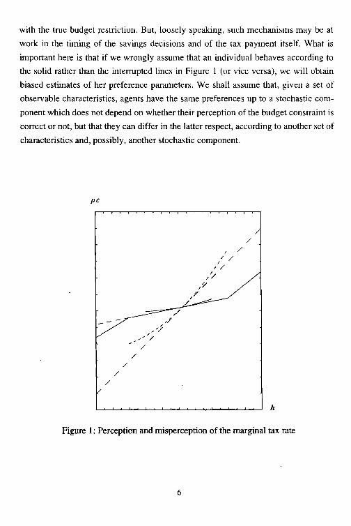
with the true budget restriction. But, loosely speaking, such mechanisms may be at

work in the timing of the savings decisions and of the tax payment itself. What is

important here is that if we wrongly assume that an individual behaves according to

the solid rather than the interrupted lines in Figure 1 (or vice versa), we will obtain

biased estimates of her preference parameters. We shall assume that, given a set of

observable characteristics, agents have the same preferences up to a stochastic com­

ponent which does not depend on whether their perception of the budget constraint is

correct or not, but that they can differ in the latter respect, according to another set of

characteristics and, possibly, another stochastic component.

pc

I/ /

// /

///~

/1'/

/,,/

,//",,,/

//

/

//

/

//

h

Figure 1: Perception and misperception of the marginal tax rate

6

In terms of our definition of perception of marginal taxes the following empirical

approaches have three common features: (i) They give up the maintained hypothesis

that the true position of the budget constraint is known, (ii) the perceived budget

constrained is endogenous and depends on individual characteristics and (iii) the

approaches nest the two extreme cases of perfect knowledge case and the complete

ignorance. The differences lie in the assumptions about the underlying preference

structure, in the stochastics and in the computational burden.

An appealing and simple way to extend the neoclassical labour supply framework in

the direction sketched above is to introduce interaction terms with the marginal tax

rate. Given the situation in the German data, where consumption is not observed, an

interesting starting point which is described in more detail by Laisney et al. (1993) is

a life cycle labour supply model based on additive intertemporal preferences where

contemporaneous preferences are quasi-linear (indifference curves are parallel). This

implies that there is no income effect on leisure. Moreover, regardless of the normal­

ization chosen for within-period preferences, hours supplied will be independent of

assets in period 0, interest rates and the rate of time preference. This is of course an

extremely restrictive set of assumptions, but given the complexity of the estimation

strategy pursued here, it will provide a convenient benchmark. In that case Frisch

demands for leisure correspond exactly with Hicksian and with Marshallian demands

and depend only on the real wage. Yet, since static models of female labour supply

typically yield small income elasticities, this may not be such a bad model. In detail,

the period t utility function is specified as

U,CC"L,) =F,[C, +V,CL,)] =:F,[U;CC"L,)],

for some increasing functions Frand Vr, where C,: denotes household aggregate con­

sumption in period t, and L, denotes the desired leisure of the female in period t. We

specify the parsimonious parametric form Box-Cox functional form VtCLt ) =YtLt{P},

withL {P}:= (L P- 1)1~ if~ ~ 0, lnL otherwise. Utility increasing in leisure requires 'Y, > 0.

This is easily achieved in estimation by specifying a logarithmic equation for this taste

shifter. Convexity of indifference curves requires ~ < 1. Using the following specifi­

cation for the taste shifter and the gross wage

7

and the condition that a woman chooses hours equating her MRS and her perceived

net wage, this results in the following form for an interior solution in desired leisure:

z~ +£1 =-(~ -1) In([ -N) + InW +aIn{1 - -r(Y, WN)}. (2.1)

Here L denotes the amount of time available for allocation between market time and

'leisure', N are the desired hours of work of the individual, Y is her husband's income,

exogenous, and W is her gross wage rate, assumed exogenous. -r denotes the marginal

tax rate, which is in Germany a function of the individual's earnings and of the other

income of the household, here her husand's income. a denotes an essential house­

hold-specific multiplier for this study: its presence corresponds to taking account of a

"subjective" marginal retention rate p. defined by p. = (l--r)u. In the following the

perception rate a depends on a vector of socio-economic characteristics, V, that may

proxy the individual's knowledge about the tax system. Assuming linearity we have

a =Vr, where r is a parameter vector to be estimated. For a =1 condition (2.1) reflects

the supply condition under perfect knowledge about marginal wage rates. Given a =0

we are in the framework where marginal tax rates are completely ignored. However,

in this approach we do not restrict a to lie between 0 and 1. Thus a negative a would

lead to a retention rate above one and a > 1would indicate an 'exaggeration' ofmarginal

tax rates.

Our econometric treatment of observations with missing wage information, or with

irregular employment or unemployment takes care of some of the problems that

availability of detailed information on demand conditions might help to handle more

explicitly. Actual hours, but also the desired hours available in our data, are influenced

by the availability of the corresponding (hours, wage) offers. It is also apparent from

a histogram of these desired hours (reproduced in Laisney et al. 1993), that most

respondents give answers that are multiples of5. We shall cope with this by considering

ranges of desired hours as the observed dependent variable rather than the actual level

8

of desired hours. This technique is used by Blundell et al. (1993) but we are in a better

position to use it here, because we do not have to make their assumption that actual

and desired hours fall into the same interval.

3 Data

3.1 German data: sample selection and description of variables

We use the unbalanced sample from Laisney et al. (1993). The selection is summarized

in Table 3.1. In order to avoid the non-convexity of the budget set caused by means­

tested benefits, we restricted the sample used in the estimation to females who would

not be entitled to the means-tested benefits giving rise to a marginal tax rate of 100%

at zero hours. This selection rule only depends on the "unearned income" and on the

demographics ofthe household, and is exogenous in the framework ofour assumptions.

Table 3.1: Sample Selection

1985 1986 1987 1988 1989

all females with valid interview 5631 5378 5308 5068 4930

German nationality 4287 4090 4010 3774 3586

age 25 - 57 2434 2328 2262 2129 2038

married and living together with partner 1903 1781 1736 1633 1555

no partner change, marriage, divorce, etc..

1846 1726 1669 1582 1510

head or wife of head of household 1842 1717 1656 1575 1499

no other adults in household 1842 1717 1656 1574 1499

not self-employed 1734 1621 1548 1477 1411

after deleting missing values..

1530 1419 1361 1266 1192

no benefits at zero hour~ 1328 1237 1193 1139 1068

* in last 18 months

** except hours and female income information

We refer the reader to Laisney et al. (1993) for the description of the variables used in

the determination of the form of the budget set of each household, since this represents

a large portion of that paper.

9

Gross wages for the participants have been computed as reported gross monthly

earnings of the last month divided by reponed average working hours (per week) of

the last month multiplied by 4.3. The resulting number is multiplied by 13/12 in order

to account for the additional income component corresponding to the "thirteenth month"

practice. In our final sample we consider observations in the lower and the upper

percentile of the wage distribution as indicating unplausible values for either the

working hours or the gross monthly income. Moreover, we discard the information on

wages for several particular groups of observations and treat them like the job seekers,

for whom the only information we use is the fact that their desired hours are positive.

The variables used in estimation may be summarily described as follows (see Table

3.2 for some descriptive statistics). Wages: real gross wage =gross wage / price index.

Hours: desired, forparticipants: nonnal weekly hours over the year; observed, including

overtime, for the computation of gross wages. These are average weekly hours over

the year.

Non-participants: women who report being registered as unemployed, or being out of

the labour force and, in case they answered yes to the question "future participation

(yes, perhaps, no)", declared that they do not look for a job that would begin

immediately. Seekers: women who report being registered as unemployed, or being

out of the labour force and, in case they answered yes to the question "future partici­

pation (yes, perhaps, no)" declared that they do look for a job that would begin

immediately. Participants: women who report working full- or part-time, or being in

vocational training, or working irregularly, or who report positive desired hours or

positive observed hours. Participants with missing wage information: Participants with

missing information on earnings or on observed hours or on desired hours, or working

irregularly, or reporting to work full time but with average weekly hours below 20, or

reporting to work part time but with average weekly hours above 35, or with computed

gross nominal wage in the upper or lower 5% of the distribution. We thus have four

categories of observations: non-participants, seekers, participants with missing infor­

mation, and participants with complete information.

Age: Woman's age in years (year of wave - year of birth), divided by 10. The square

ofthe same variable is used also. Schooling: Three dummies for highest grade in general

10

Table 3.2: Descriptive statistics: Germany

Year 1985 1986 1987 1988 1989

Variable mean std mean std mean std mean std mean std

price index 1 0 0.998 0 0.999 0 1.01 0 1.039 0non-participants 0.49 0.49 0.48 0.48 0.47seekers 0.03 0.04 0.04 0.02 0.04participants 0.48 0.46 0.47 0.49 0.50part., no wage information 0.13 0.13 0.11 0.11 0.13real hourly wage (OM 1985)* 14.9 5.41 16.0 7.67 16.1 6.3 17.0 7.05 17.0 7.00desired weekly hours* 25.4 9.64 26.1 8.73 26.9 9.10 25.5 8.85 26.5 8.91actual weekly hours* 30.4 11.2 32.0 11.2 30.2 11.3 29.4 11.7 29.9 10.8

age 41.1 9.01 41.5 8.99 41.5 8.90 41.5 8.91 41.4 8.94disability 0.03 0.15 0.04 0.14 0.04 0.16 0.04 0.15 0.04 0.15potential experience 25.8 9.32 26.5 9.15 26.7 8.78 27.1 9.00 27.3 8.06

schooling: highest degreeHauptschlfle, or no degree 0.70 0.71 0.71 0.72 0.72Realschule 0.22 0.21 0.21 0.21 0.21Fachoberschule, Abitur 0.08 0.08 0.08 0.07 0.07

children:youngestichild 0-2 years 0.10 0.11 0.10 0.09 0.07

II II 3-5 " 0.12 0.11 0.12 0.13 0.14" 6-11 " 0.16 0.16 0.16 0.17 0.18" 12-15 " 0.15 0.14 0.12 0.10 0.09" 16-25 0.25 0.26 0.28 0.28 0.30

number of children 0-5 0.27 0.55 0.29 0.59 0.27 0.55 0.27 0.55 0.24 0.51" 6-11 0.30 0.56 0.31 0.58 0.33 0.62 0.35 0.63 0.36 0.64" 12-15 0.26 0.50 0.23 0.48 0.21 0.46 0.20 0.45 0.19 0.43" 16-25 0.58 0.84 0.57 0.82 0.58 0.82 0.58 0.83 0.60 0.81

regional variablesnorthern states 0.19 0.19 0.19 0.18 0.19Nordrhein-Westfalen 0.28 0.28 0.28 0.29 0.29Berlin 0.03 0.03 0.03 0.03 0.02central states 0.16 0.17 0.16 0.16 0.17Bayern, Baden-Wiirttemberg 0.33 0.34 0.34 0.34 0.33

Urbanisation (areas)more than 500' inhabit. 0.44 0.44 0.44 0.43 0.43

100' - 500' 0.15 0.16 0.16 0.16 0.1620' - 100' 0'.11 0.11 0.11 0.11 0.11less than 20' 0.30 0.29 0.29 0.29 0.29

Parameters of tax approxmarginal tax rate at zero hours 0.15 0.07 0.15 0.07 0.15 0.07 0.16 0.07 0.16 0.07margo tax rate at desired hours 0.29 0.19 0.29 0.18 0.30 0.18 0.29 0.17 0.30 0.17benefits at zero hours: dummy 0.13 0.11 0.13 0.11 0.10

* participants with "accepted" wage rates only

11

education, corresponding to (years of schooling in brackets) "Hauptschule" (9)

"Mittlere Reife" (10) "Abitur" or "Zulassung zur Fachhochschule" (13 and 12,

respectively). Potential experience: (Age - Years of schooling - 6) / 10. The square is

also used. Children: (i) Numbers of children: up to 5 years of age, between 6 and 11,

between 12 and 15, older than 15 and still in education. (ii) Dummies youngest child:

up to 2 years of age, between 3 and 5, between 6 and 11, between 12 and 15, older than

15 and still in education. Urbanization grade (Boustedt): Town, village, rural (below

20' inhabitants).

3.2 French data: sample selection and description of variables

We work with the subsample of 3658 households from the INSEE survey "Budgets

des Familles 1979" already used by Laisney et al. (1991) and Blundell et al. (1993).

The selection was made according to the following criteria: we consider single tax units

based on a married couple where the male is either working or, ifpresently out of work,

is seeking a job. The household has no other wage earner than the husband or the wife.

The latter is neither at school nor is a student or a pensioner or an 'aide familiale' , she

is neither self-employed nor a teacher or an artist or a member of clergy, army or police.

She is between 26 and 65 years'of age and reports at most 69 normal weekly hours of

work. Since means-tested benefits are assessed on the taxable income of the previous

year, we only take taxes in a strict sense proper into account in this first approach. We

now summarily describe the variables used (age and potential experience have the same

definition as for the German data). Wages: gross wages for the participants have been

computed as reported gross yearly earnings (including bonuses) divided by reported

normal weekly working hours times 52. Hours: reported normal weekly hours of work.

Seekers: unemployed and women who do not participate at the time of the interview

but who report that they are currently looking for a job. Participants: only women who

report positive hours. Non-participants: women who do not belong to either of the

previous categories. We thus have only three categories of observations for the French

data.

12

zewSchooling: three dummies for highest grade in general education, corresponding to end

of primary school (BE), mid secondary school (BEPC), end of secondary school or

above (baccalaureat). Numbers of children: (i) not yet in the next category, (ii) at the

"ecole matemelle" (kindergarden), (iii) dummies for the numbers ofchildren at primary

and secondary school (1, 2, 3 or more). Marginal tax rate: the approach here is simpler

than for the German data and makes the assumption of constancy of the marginal tax

rate over the relevant range of hours. For the French data this is an acceptable

approxim~tion (see Blundell et al. 1993 for details).

Table 3.3: Descriptive statistics: France 1978/1979

non-participants 0.52participants 0.43seekers 0.05gross nominal hourly wage (FF)* 17.7normal weekly hours (actual)* 36.6

age 39.6potential experience 23.1regional unemployment rate 0.06telephone (dummy) 0.63

schooling: highest degreenone 0.28end primary school (BE) 0.43mid secondary school (BEPC) 0.18end secondary school (baccalaureat) or above 0.11

numbers of children:small 0.18ecole maternelle 0.22dummy one other chilq 0.26dummy two other children 0.23three or more other children 0.14

suburb 0.39

marginal tax rate 0.23

* participants only

13

std

7.59.6

9.59.7

0.01

0.430.49

0.07

min

2.003

263

0.05

oo

0.09

max

56.666

6549

0.10

33

0.50

4 ResultsDue to a substantial clustering of hours in both samples we restrict our attention to a

model specification where hours information is grouped according to the cut-points

22.5, 27.5, 32.5, 37.5 hours per week. The choice of these cut-points is justified in

Laisney et al. (1993). For the German panel data we estimate the model for all five

cross-sections by maximum likelihood and use the' minimum distance estimation

technique to enforce the panel structure on the cross-section estimates. In Table 4.1 we

present two sets of estimates for Germany, according to whether or not we restrict the

variance of the taste shifter to 1. Table 4.2 presents the corresponding maximum

likelihood results for the French cross-section. Both sets of results are based on the

choice ofL =10.5 hours a day.!

A first feature of the results is that estimates of the wage elasticity of leisure are fairly

high in absolute terms compared to the results of previous studies using the same data

(Laisney et al., 1993, and Hujer and Schnabel, 1992, for Germany; Dagsvik et al., 1988,

and Blundell et al., 1993, for France).

In many respects the estimates for Germany seem more reliable than the results for

France and we discuss these first. The parameters of the wage equation and the taste

shifter are fairly standard. The (log-) wage profile is bell-shaped in terms of potential

experience, with a maximum at 22 years of experience. In interpreting the coefficients

in the taste shifter it must be remembered that a positive impact on the taste shifter

increases the weight of leisure in the utility function. Having children in any of the

defined age groups implies a reduction of hours supplied.

Most interesting for the present study are the results obtained for the coefficients

appearing in the perception rate. In terms of our model, positive coefficients on the

different child dummies in V indicate that women with children are likely to have a

higherperceptionofthe marginal tax rate. We offer the following tentative explanations

for this finding. If families with children find it more difficult than childless couples

I In opposition with most of the literature on this point, we find that this choice does matter. Ideally,one would want to allow r to vary with demographics, but this would strain identification one stepfurther than we already do. For the German data, the value of 10.5 corresponds approximately to anestimate obtained by restraining (l to be equal to 1.

14

to make ends meet, they may be more inclined to take into account their true marginal

tax rate. Moreover, having access to special tax allowances for families with children

may produce a better knowledge about the true tax rate. However, this argument is not

supported by our finding that owning a house, and thus possibly receiving corre­

sponding tax reductions, has no significant impact on the perception rate. The neo­

classical assumption that individuals are perfectly aware ofthe implications ofmarginal

tax rates appears more likely to hold for women with a higher educational degree than

for the reference group.

The estimates for France differ to some extent from previous results. This holds for

the wage equation, where we do not find a significant impact of potential experience

on wages; furthermore, the coefficients on the child dummies appearing in V are not

well determined and are negative in contrast to the results obtained with the German

data. Education has the expected positive sign. The impact of age on the perception

rate is concave with a maximum at age 48, whereas we find no such effect for Germany.

The dummy variable for the ownership of a telephone was included to pick up potential

differences in information. Its positive impact on wages and the perception rate might

also pick up an income effect. Although the results for France appear robust with respect

to inclusion of this variable, they are very fragile as far as other modifications of the

specification are concerned: since the specification reported here is derived from the

final specification retained for the German data, we have good reasons to suspect it to

fit the French data less well. Experimenting with changes in the level ofr, we found

thatr =15 led to a lower elasticity but to even more negative values of a than implied

by the estimates reported here. When changing the grouping of hours we encountered

difficulties with convergence.2 Due to this instability and to the better quality of the

German data as regards the evaluation of marginal tax rates, we concentrate on the

implications of the estin,tated model for Germany. We will come back to the French

data when discussing models which take advantage of the availability of information

on expenditures.

2 We also had convergence problems when trying to produce results with a constant across individualswhile retaining the same specification for the preferences, as done by Rosen (1976b): the resultingmodel was obviously underparameterized, which again points to the identification issue discussedabove.

15

Table 4.1: Gennany: Minimum Distance Estimation, Unbalanced Panel,Results with and without Restriction on Variance of Taste Shifter (*: std. err)

Restriction (Yes/No) No Yescoef. t-value coef. t-value

~Wage equation

Taste shifter

Variables in V

Covariancestructure

constant 1985constant 1986constant 1987constant 1988constant 1989potential experience /10pot. experience squared /1000less than 20' inhabitantsRealschuleFachoberschule, Abiturconstant 1985constant 1986constant 1987constant 1988constant 1989number of children 0-5

II II 6-11II 12-15II 16-25

constant 1985constant 1986constant 1987constant 1988constant 1989youngest child 0-2 years

11 II 3-5 "II 6-11 II

II 12-15 II

RealschuleFachoberschule, Abitur

0'1 1985

0'1 1986

0'1 1987

0'1 19880'1 1989

P 1985P 1986P 1987P 1988P 19890'2 1985

0'2 1986

0'2 1987

0'2 1988

0'2 1989

16

0.7152.4952.5602.6002.6242.6470.171-0.5150.0110.1540.2814.6544.7294.7754.7824.8420.2460.1350.0800.0490.0430.002-0.095-0.010-0.1700.184-0.0080.1310.0740.2250.3520.4300.456

0.4160.415

0.351

0.7370.8280.7980.8170.7770.341

0.375

0.366

0.3800.368

11.(534.034.934.433.833.83.1-4.90.66.06.09.9

10.010.210.210.36.05.12.72.40.60.0-1.3-0.1-1.61.9-0.11.91.04.44.1

0.052*0.045

0.0570.055

0.059

0.0660.0510.0600.0600.065

0.0130.019

0.015

0.0160.016

-0.0292.2792.3722.3842.4102.4330.299-0.691-0.0440.2380.50110.21610.34610.34710.32710.3990.5930.3180.2000.1890.082

-0.043-0.1960.096-0.1590.576 '0.0100.3460.2910.3740.575

1

1

11

1

0.3270.4980.4780.4830.4890.328

0.368

0.359

0.377

0.356

-0.526.227.227.427.027.34.6-5.5-1.89.312.823.724.024.224.023.911.48.04.06.20.6

-0.3-1.70.7

-1.23.70.13.02.24.44.0

0.074*0.0610.0650.0680.067

0.0130.019

0.014

0.0150.016

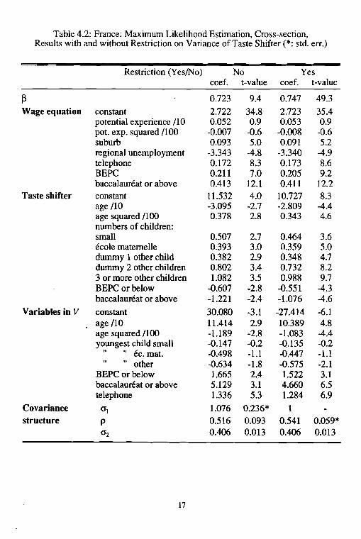
Table 4.2: France: Maximum Likelihood Estimation, Cross-section,Results with and without Restriction on Variance of Taste Shifter (*: std. err.)

Restriction (Yes/No) No Yescoef. t-value coef. t-value

~ 0.723 9.4 0.747 49.3

Wage equation constant 2.722 34.8 2.723 35.4potential experience /10 0.052 0.9 0.053 0.9pot. expo squared /100 -0.007 -0.6 -0.008 -0.6suburb 0.093 5.0 0.091 5.2regional unemployment -3.343 -4.8 -3.340 -4.9telephone 0.172 8.3 0.173 8.6BEPC 0.211 7.0 0.205 9.2baccalam-eat or above 0.413 12.1 0.411 12.2

Taste shifter constant 11.532 4.0 10.727 8.3age /10 -3.095 -2.7 -2.809 -4.4age squared /H)O 0.378 2.8 0.343 4.6numbers of children:small 0.507 2.7 0.464 3.6ecole matemelle 0.393 3.0 0.359 5.0dummy 1 other child 0.382 2.9 0.348 4.7dummy 2 other children 0.802 3.4 0.732 8.23 or more other children 1.082 3.5 0.988 9.7BEPC or below -0.607 -2.8 -0.551 -4.3baccalaureat or above -1.221 -2.4 -1.076 -4.6

Variables in V constant 30.080 -3.1 -27.414 -6.1age /10 11.414 2.9 10.389 4.8age squared /100 -1.189 -2.8 -1.083 -4.4youngest child small -0.147 -0.2 -0.135 -0.2

" "ec. mat. -0.498 -1.1 -0.447 -1.1" other -0.634 -1.8 -0.575 -2.1

BEPC or below 1.665 2.4 1.522 3.1baccalaureat or above 5.129 3.1 4.660 6.5telephone 1.336 5.3 1.284 6.9

Covariance (JI 1.076 0.236* 1structure p 0.516 0.093 0.541 0.059*

(J2 0.406 0.013 0.406 0.013

17

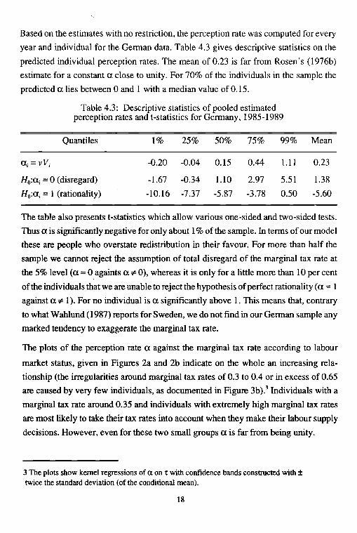
Based on the estimates with no restriction, the perception rate was computed for every

year and individual for the German data. Table 4.3 gives descriptive statistics on the

predicted individual perception rates. The mean of 0.23 is far from Rosen's (1976b)

estimate for a constant a close to unity. For 70% of the individuals in the sample the

predicted a lies between 0 and 1 with a median value of 0.15.

Table 4.3: Descriptive statistics of pooled estimatedperception rates and t-statistics for Gennany, 1985-1989

Quantiles 1% 25% 50% 75% 99% Mean

aj=vVj -0.20 -0.04 0.15 0.44 1.11 0.23

HO:a i = 0 (disregard) -1.67 -0.34 1.10 2.97 5.51 1.38

Ho:a j = 1 (rationality) -10.16 -7.37 -5.87 -3.78 0.50 -5.60

The table also presents t-statistics which allow various one-sided and two-sided tests.

Thus a is significantly negative for only about 1% of the sample. In tenns of our model

these are people who overstate redistribution in their favour. For more than half the

sample we cannot reject the assumption of total disregard of the marginal tax rate at

the 5% level (a =0 againts a "# 0), whereas it is only for a little more than 10 per cent

of the individuals that we are unable to reject the hypothesis ofperfect rationality (a =1

against a "# 1). For no individual is a significantly above 1. This means that, contrary

to what Wahlund (1987) reports for Sweden, we do not find in our Gennan sample any

marked tendency to exaggerate the marginal tax rate.

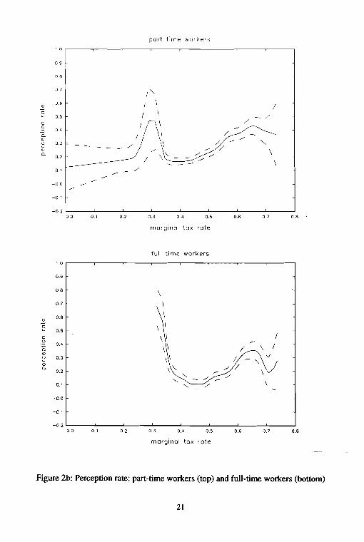
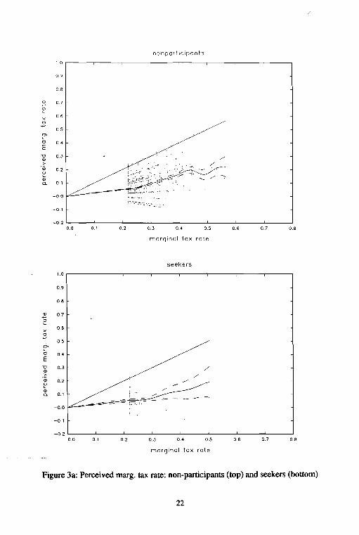
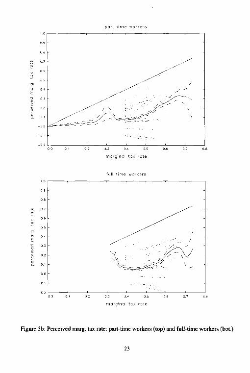
The plots of the perception rate a against the marginal tax rate according to labour

market status, given in Figures 2a and 2b indicate on the whole an increasing rela­

tionship (the irregularities around marginal tax rates of 0.3 to 0.4 or in excess of 0.65

are caused by very few individuals, as documented in Figure 3b).3 Individuals with a

marginal tax rate around 0.35 and individuals with extremely high marginal tax rates

are most likely to take their tax rates into account when they make their labour supply

decisions. However, even for these two small groups a is far from being unity.

3 The plots show kernel regressions of a on 't with confidence bands constructed with ±twice the standard deviation (of the conditional mean).

18

Comparing across groups, we find that the perception ofpart-time workers seems more

accurate than that of full-time workers, which is consistent with the higher education,

on average, of part-time workers, and that seekers have a flatter profile than non par­

ticipants.

For individuals with zero marginal tax rate, whatever their labour market position, the

question of misperception of the marginal tax rate is without any importance for the

labour supply decision since at a tax rate of zero the impact of the misperception on

hours supplied is nil, at least in our model.

Therefore it is interesting to look at the relationship between the actual marginal tax

rate t and the perceived marginal tax rate t·, where the latter is defined by the relation

(l-t)U = I -t·, and represents the tax rate that would produce the same behaviour if

exactly perceived. This relationship is depicted in Figures 3a and 3b, where on top of

the kernel plots we have also represented each individual point (t, t·). The clustering

of values of t around some of the lower values correspond to tax allowances and to an

allowance for the payment of social contributions (see Laisney et aI., 1993, for details).

The solid straight line shows equality between t and t·, or perfect perception.

One way to look at the pictures is to ask what the perceived marginal tax rate is on

average for a given marginal tax rate of, say 0.45. Thatvalue is 0.18 for non participants,

0.14 for seekers, 0.08 for part-timers and 0.06 for full-timers. It is small, but the relative

magnitudes are in intuitive accordance with the observed labour market status. How­

ever, it is worth noting also that a possible explanation for this ranking could lie in the

fact that our model takes no account of the "investment in human capital" aspect of

market work.

19

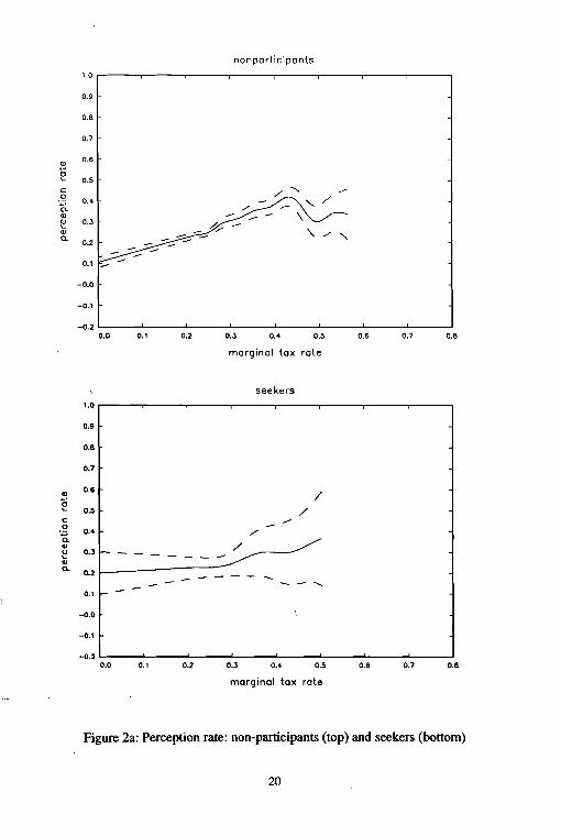
Figure 2a: Perception rate: non-participants (top) and seekers (bottom)

20

part time workers

1.0

0.9

08

0.7/""-

0>0.5 I \

/"2 05 I \

/c \ ./0

04 /0- f \ /0>

0.3 \ / ""-c> ./ '/0> \0- \" ./0.2

./\

01

-0 a

-0 1

-0.200 0.1 0.2 0.3 0.4 0.5 0.6 0.7 O.B

marginal tax rate

full time workers

1.0

0.9

0.8\

0.7 \

0.6 \

.2\2 0.5 \

c \ \ /0

0.4\ \ / \ f

0-0>

\ \ vc> 0.3 / '\0>

"./ /0-

\0.2""- --./ ./

"- - -- \0.1 "'- ./

-00

-0 1

-0200 0.1 02 0.3 0.4 0.5 0.6 0.7 O.B

marginal tax rate

Figure 2b: Perception rate: part-time workers (top) and full-time workers (bottom)

21

nonparticipants

1 0 r------r-----,-----r-------,---..,---------,,----------,-------,

0.9

0.8

0.7

x.::;

06

0.5

~o 0.4E\J 0.3<lJ.~

<lJ 0.2~<lJa. 0.1

-0.0

-0.1

/

-0.2 L.-...__.....L ....l.... l...-__......L.. ...l..-__........I ......L..__---l

0.0 0.1 0.2 0.3 0.4 0.5 0.6 0.7 O.B

marginal tax rate

seekers

1.0 r-------,---..,--------,---...,---.,-------r-----r-----,

0.9

0.8

0.7

x.::;

0.6

0.5

~o 0.4E\J 0.3<lJ>

'(jj 0.2

~<lJa. 0.1

-0.0

-0.1

/

-0.2 l...-__......L.. ...l..-__---l ....L.. ..L...-__.......L ....I....__---l

0.0 0.1 0.2 0.3 0.4 0.5 0.6 0.7 0.8

marginal tax rate

Figure 3a: Perceived margo tax rate: non-participants (top) and seekers (bottom)

22

part time workers

/~/'

/.'/'" .._-::.~.:~/­

-;:::-~-,~ .. _.v· ... ~::::.·,;:-:

/

/'

./

/' ""-\

\

1.0

0.9

08

2 0.7

;:x 06

0

05

2'0 0.4E"D 0.3<j)

.:::<j) 0.2~<j)

o 1Q.

-00

-D 1

-0200 0.1 0.2

/ ""­/ \

0.3 0.4 0.5 D.6 0.7 O.B

marginal tax rate

full time workers

./'~/

z;/~",:~.. ,....

1.0

09

08

2 0.7

;:x

06

2D5

2'0 04E

"D 0.3QJ

.:::QJ D.2~QJ

0.1Q.

-D a

-0 1

-D 200 0.1 02 03 0.4 0.5 06

\

\

0.7

I

/

D.B

marginal tax rate

Figure 3b: Perceived margo tax. rate: part-time workers (top) and full-time workers (bot.)

23

5 Alternative Approaches

5.1 Theoretical Model and Previous Results

We start with no taxes and with the standard problem of one individual with inter­

temporally separable preferences who maximizes expected discounted utility

over the life cycle, subject to

(5.1)

(no bequest)

k=t, ... ,T-l (5.2)

in self-explaining notation, and with uncertainty limited to the (gross) wage and interest

rate profiles. Using the Bellman principle, we define

T

Vt + 1 =maxE L ~kU(ck,hk) s.t.(2)fork=t+l, ... ,T. (5.3)t+lk=/+1

The only choice variable entering Vt+ 1 is At , and

(5.4)

subject to

(5.5)

Thus, conditioning on A, , the current period decision variables c, and h, are solutions

of

and the fonn of the constraint in (5.6) stresses the relevance of "dissaving" IJ.t as

conditioning variable. This will allow us to omit the time periodsubscript tin the sequel.

In a model with taxes, the constraints (5.2) are replaced by

24

Ak = (1 + rk)Ak: 1+Yk +wkhk- PkCk -/(hk, Yk' rk,Ak_I,Ak) (5.7)

with 1(.) a general tax function. An approximation (exactly valid over some range of

hours for a piecewise linear budget restriction) is obtained by linearizing the budget

constraint, using the "net" counterparts of Yt , rt , and WI:

(5.8)

Hence the definition of the "net" dissaving variable

(5.9)

Thus for given (pc, h) and w (or W *), Jl (or Jl*) is obtained from the relevant (linearized)

budget constraint.4

Finally, going over to the households we shall be interested in subsequently, namely

households based on a married couple, the analysis goes through under the assumption

that male leisure is both separable from female leisure and consumption and con­

strained. The only change necessary is a redefinition of the unearned income variable

Y so as to include the male's earnings.

The preference specification we use here is described in detail in Blundell et al. (1993).

Here it will suffice to say that it leads to the following labour supply equation:

h = (l - ~)y+ ~(d - Jl)/w , (5.10)

with a nonnal stochastic component appearing additively in y. This interpretation of

the stochastic component in tenns of random preferences only will simplify the

exposition without introducing significant restrictions. Since the labour supply function

(5.10) includes the "net" dissaving variableJl we are only able to estimate the model

for the French data which include infonnation on expenditures.

4 A more detailed analysis of the case of a nonlinear tax function and a justification of the procedurefollowed here are given by Blomquist (1985).

25

Since the study of Blundell et al. gives some grounds to distrust the hours information

available in the data used, we shall concentrate on the participation rather than on the

full labour supply decision. In doing so we lose information which may help identifying

the preference parameters, but on the other hand we discard one potential source of

misspecificat'on. Other potential sources of misspecification are errors in variables,

simultaneity bias, and fixed costs of participation. Errors in variables and endogeneity

in both wages and dissaving are, to some extent, taken care of by the use of instrumental

variables. Fixed costs of work may be more problematic since these are included in

the consumption of participants but are unobserved for non-participants.

Table 5.1 shows probit estimates for the participation condition derived from (5.10).

The first pair of columns relates to the assumption that every woman in the sample

considers the complete tax system, including benefits and social security contributions,

while the second sets the marginal tax rate to zero and corresponds to a linear budget

constraint. Assuming that everyone disregards her marginal tax rate leads to much

stronger wage effects. Another striking difference is the reversal on the impact of

education on participation, and the very different estimates for the minimum

expenditures, which are identified from a probit model (three last lines of the table).

See Blundell et al. for more details.

The diagnostics reported in Table 5.2 show a trade-off between the specification of the

marginal tax rate and non-linearity in the preferences: linearity is passed easily for the

model with complete treatment of the tax system only. The deterioration of the hete­

roscedasticity diagnostic for the inverse of the marginal wage reinforces this finding,

which is no surprise since that diagnostic picks up a special type of non-linearity.

26

Table 5.1 Probit estimates with identical perception of the tax systemfor all households.

Model marginal wage rate gross wage rate

Variable coeff. t-val. coeff. t-val.

intercept 0.8246 3.3162 2.7082 10.8132(age-40)/10 -0.3812 -11.5598 -0.3601 -10.5605same, squared -0.1310 -4.3122 -0.1237 -4.0230primary school 0.2909 5.1043 0.1941 3.2905lower secondary 0.4548 5.3075 -0.0412 -0.4470end secondary 0.3623 3.0921 -0.3322 -2.6525higher education 0.2863 2.0110 -0.3482 -2.3681small children -0.6878 -10.4453 -0.5634 -8.2270ecole matemelle -0.4793 -9.3007 -0.3599 -6.6668one other child -0.2481 -3.9844 -0.1018 -1.6071two other children -0.6666 -9.0512 -0.3657 -4.7561> 2 other children -0.9137 -10.1181 -0.3510 -3.5295suburb dummy 0.1610 3.3477 0.0008 0.01721/marg. wage [l/w] 2.3854 0.9246 -16.7075 -5.3414owner/w -0.9884 -1.0722 0.2224 0.1826buyer/w 2.1465 3.4361 2.8566 3.4540rn/w -1.5684 -8.4054 -4.0566 -14.0549

-2*Log Lik. 4397 4182

Table 5.2 Diagnostics: empirical significance levels (%).

Model

QLM - Test

linearitym2

w2

lnw

homoscedasticity(age-40)/10end secondaryl/marginal wage [1/w]

normalityskewnesskurtosis

d.oJ.

3111

16111

211

marginal wage rate

35.96536.32215.82920.083

0.0121.2750.0110.464

20.6458.283

80.828

27

gross wage rate

0.0000.0000.0000.000

0.01239.8520.0030.051

6.99710.9003.936

5.2 Two Alternative Statistical Models

5.2.1 Switching Regressions

In this approach we consider that each individual has some probability 7t to take her

true marginal tax rate into account and probability 1-7t to disregard it fully. Given that

(5.9) is written with different versions of w and ~ in each case, but with the same error

tenn, the model will have the following structure:

(5.11 )

z·=.Zc-v,

where u and v are jointly nonnal with variances set equal to 1 and correlation p . The

nonnalisation of the variances corresponds to the usual lack of identification in

dichotomous models. The latent variable y. coincides with y; in regime 1, that is, if

z· ~ 0, and with y; otherwise. The observed dichotomous variable y is defined as

y =1[y. ~ 0] . Thus the participation probability is given by

p=P[y=l]=P[y;~O 1\ z·~O] + P[y;~O 1\ z·<O] (5.12)

=P [u 5: XIb 1\ V 5: Zc ] + P [u 5: X2b 1\ v > ZC ]

where <1>(2) denotes the cumulative of the bivariate nonnal. If p =0 this simplifies to:

In any case the log-likelihood function for an i.i.d. n-sample takes the fonn

n

lnL(y IX,b,c,p)= L[y;lnp;+(l-yJln(l-pJ];=1

with score vector given by

28

(5.13)

(5.14)

and

dlnL Yi - Pi

dPi =Pi(1 - p;)

dP , ,db =<!>(X1b )<t>(Ze - pX1b )X1+ <!>(X2b) [1- <t>(Ze - pX2b)]X2

dp .de =<!>(Ze) [<t>(X1b - pZe) -<t>(X2b - pZe)]Z

(5.15)

(5.16)

the latter relationship being given in Hausman and Wise (1978, fn.17). There does not

appear to be any theoretical identification problem in either case, except in some

pathological cases. For instance, if Xl =X2, Yis not identified. It is however clear that

the model puts great strain on the data (see Kiefer, 1979). The Appendix reports on

limited experimentation with simulated data using this model. This yields the following

conclusions, which would need to be checked with a thorough Monte-Carlo study. 1

Convergence is obtained easily using numerical gradients but is often difficult with

analytical gradients. The explanation seems to lie in insufficient precision in the

computation of the univariate and bivariate cumulative probability functions for the

normal. 2 Wrongly assuming that p =0 causes little bias in the estimation of b as long

as p is not too large. 3 The number of observations necessary for precise estimation of

the parameters e of the switching process is much larger than that giving precise

estimation for the preference parameters b. Precise estimation of p requires even more

observations.

5.2.2 Convex Combination Approach: Nonlinear Probit

The basic idea of the following convex combination approach is to treat wages and

nonwage income perceived by the individual as a convex combination of the two

extreme cases: The rational perception of the budget constraint's curvature and the

complete disregard of marginal wage rates. Assuming that the individual's perception

of the budget constraint is given by:

29

(5.17)

where the superscript p denotes the individual's perception of the corresponding

variable. This perception is expressed as weighted average of the two extreme cases.

For the perceived wage rate this is given as the weighted average of the marginal wage,

w· , and the gross wage, W . More precisely, if \jI denotes the relative weight given to

"rational" tax behaviour, w P is defined as:

(5.18)

The perceived nonlabour income is defined correspondingly. Hence for \jI = I equation

(5.18) reduces to the linearized budget constraint of the conventional neoclassical

labour supply mod~l with taxes, and results in the linear budget constraint of an indi­

vidual ignoring taxes for \jI =0. In a second step the perception weight is endogenized

by expressing \jI as a function of observable socio-economic characteristics. For our

econometric approach we assume a logistic functional fo~ for \jI in order to restrict

the weights to the interval [0,1] while keeping the computational burden low:

\jI =(1 +exp(-z 'y)r\ (5.19)

where z is a k x 1 - vector ofexplanatory variables and yis the corresponding parameter

vector to be estimated. For the quasi-homothetic preferences corresponding to (5.10)

the labour supply specification will be:

(5.20)

Since we use only binary information on hours, the convex combination approach

results in a probit model which is both parameters and variables. In comparison to the

switching probit model this model is stochastically simpler, but this does not reduce

the computational burden, because of the high degree of non-linearity implied by

equations (5.18-5.20).

The convex combination approach is not only justified as an approach that nests the

two extreme cases while being parametrically considerably richer, it also has some

theoretical justification since it can be derived from utility maximizing behaviourunder

30

uncertainty with respect to the income taxes. This, however, requires the strong

assumption that expected wages are based on a binary outcome as given by (5.18).

Since it is more likely that individuals have "some partial knowledge about their tax

rates we would prefer to refer to w P as perceived marginal wage rate rather than expected

marginal wage rate.

5.3 Estimation Results

5.3.1 Switching Regressions Model

In our first attempts at estimating the switching regressions model we did not impose

equality of all the preference parameters between regimes and assumed a constant

probability of disregard across households. This led to almost exactly the results

obtained for the gross wage rate in Table 5.1, and a probability of disregard almost

equal to 1. In a second type of attempts, we moved to the other extreme in order to

obtain some deviation from complete disregard: we retained only a constant, the inverse

of the wage and the ratio IJIw in each regime, without restrictions, while all other

variables appeared in the switching process. The results are not reproduced because

the corresponding hessian is not invertible: it has three null eigenvalues associated with

the preference parameters for the "tax" regime. Besides, the probability of participation

for the tax regime amounts to zero for almost every observation. Finally, we did impose

the restriction of identical preference parameters across regimes: a surprising conse­

quence is that the hessian now has 8 null eigenvalues, all of them being related to switch

parameters.

5.3.2 Estimation Results of the Convex Combination Approach

Estimating the convex combination model turns out to be computationally burdensome

and sensitive to the optihtization algorithm chosen. We first estimated the model

assuming all demographic variables to enter only the weighting function (5.19). The

results are presented in Table 5.3.

Several of the weighting function parameter estimates are only mildly significant, but

are, apart from the sign (the convention is different) and a factor of proportionality,

broadly in accordance with the (non-converged) parameters obtained for the switching

31

regressions (see subsection 5.3.1). Women with higher education or end secondary

education are more likely to take marginal tax rates into account when deciding upon

work force participation. The same holds for older women. More surprisingly perhaps,

but still in accordance with the intuition presented in the introduction, the variables

small children and ecole maternelle reveal a significant impact on the probability of a

rational perception of the marginal tax rate. The average estimate of the weight given

to full perception (average 'II) is 0.19 with some 15% of the individuals giving a weight

above 1/2 to complete perception of the budget constraint. The fact that most individuals

in the sample are more likely to ignore their marginal taxes is also reflected in the

estimates of the preference parameters which come close to the estimates under the no

tax assumption. In terms of the number of correct predictions this estimated model lies

between those for the participation decision under the two polar cases regarding tax

perception. The squared age variable and the suburb dummy used in Table 5.1 had to

be deleted here due to problems of convergence of the various optimization routines

applied.

In a second step we estimated a richer specification using the set of demographic

variables belonging to the utility function as well as to the weighting function (see

columns 3 and 4 of Table 5.3). For several choices of the starting values used, con­

vergence was achieved for parameter values of ythat appear at first sight as blown-up

versions of the estimates of the restricted model. Yet there are striking differences

beyond scale. Firstly, none of the coefficients of the weighting function turns out to be

significant. Secondly, the average estimate of 'II is now much smaller. Accordingly,

the preference parameters are more similar in size and significance to those from the

simple participation model based on the gross wage rate (see columns 3 and 4 of Table

5.1 for comparison).

Finally, we used the estimated parameters of the restricted model to calculate the

perceived wage rate according to equation (5.18) and estimated the borderline models

with the estimated perceived wage rate instead. The number of correct predictions

(0.691 %) is close to the figure obtained when taxes are completely ignored (0.697%)

and exceeds the figure for the full tax borderline case by roughly 2%.

32

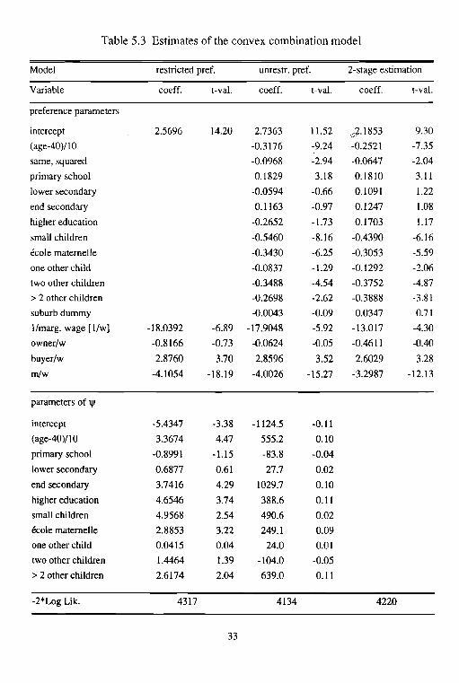
Table 5.3 Estimates of the convex combination model

Model restricted pref. unrestr. pref. 2-stage estimation

Variable coeff. t-val. coeff. t-val. coeff. t-val.

preference parameters

intercept 2.5696 14.20 2.7363 11.52 eJ·1853 9.30

(age-40)/1O -0.3176 -9.24 -0.2521 -7.35

same, squared -0.0968 -2.94 -0.0647 -2.04

primary school 0.1829 3.18 0.1810 3.11

lower secondary -0.0594 -0.66 0.1091 1.22

end secondary 0.1163 -0.97 0.1247 1.08

higher education -0.2652 -1.73 0.1703 1.17

small children -0.5460 -8.16 -0.4390 -6.16

ecole maternelle -0.3430 -6.25 -0.3053 -5.59

one other child -0.0837 -1.29 -0.1292 -2.06

two other children -0.3488 -4.54 -0.3752 -4.87

> 2 other children -0.2698 -2.62 -0.3888 -3.81

suburb dummy -0.0043 -0.09 0.0347 0.71

l/marg. wage [1/w] -18.0392 -6.89 -17.9048 -5.92 -13.017 -4.30

owner/w -0.8166 -0.73 -0.0624 -0.05 -0.4611 -0.40

buyer/w 2.8760 3.70 2.8596 3.52 2.6029 3.28

rn/w -4.1054 -18.19 -4.0026 -15.27 -3.2987 -12.13

parameters of 'II

intercept -5.4347 -3.38 -1124.5 -0.11

(age-40)/l0 3.3674 4.47 555.2 0.10

primary school -0.8991 -1.15 -83.8 -0.04

lower secondary 0.6877 0.61 27.7 0.02

end secondary 3.7416 4.29 1029.7 0.10

higher education 4.6546 3.74 388.6 0.11

small children 4.9568 2.54 490.6 0.02

ecole maternelle 2.8853 3.22 249.1 0.09

one other child 0.0415 0.04 24.0 0.01

two other children 1.4464 1.39 -104.0 -0.05

> 2 other children 2.6174 2.04 639.0 0.11

-2*Log Lik. 4317 4134 4220

33

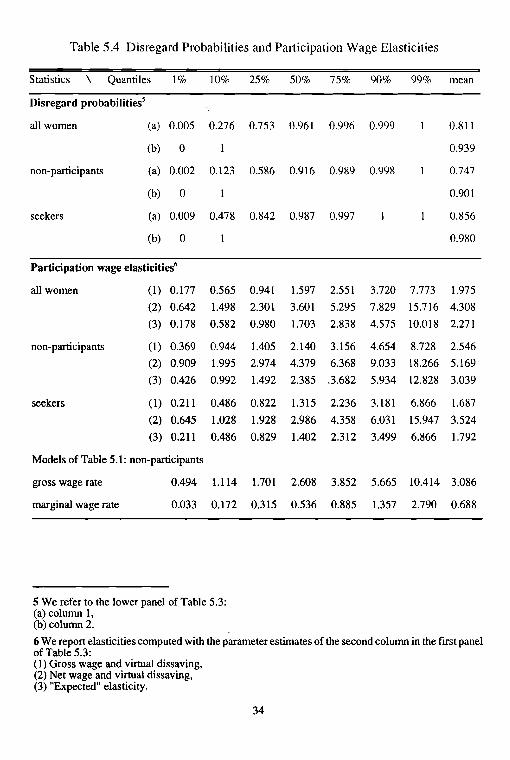
Table 5.4 Disregard Probabilities and Participation Wage Elasticities

Statistics \ Quantiles 1% 10% 25% 50% 75% 90% 99% mean

Disregard probabilities5

all women (a) 0.005 0.276 0.753 0.961 0.996 0.999 0.811

(b) 0 0.939

non-participants (a) 0.002 0.123 0.586 0.916 0.989 0.998 0.747

(b) 0 0.901

seekers (a) 0.009 0.478 0.842 0.987 0.997 0.856

(b) 0 0.980

Participation wage elasticities6

all women (1) 0.177 0.565 0.941 1.597 2.551 3.720 7.773 1.975

(2) 0.642 1.498 2.301 3.601 5.295 7.829 15.716 4.308

(3) 0.178 0.582 0.980 1.703 2.838 4.575 10.018 2.271

non-participants (1) 0.369 0.944 1.405 2.140 3.156 4.654 8.728 2.546

(2) 0.909 1.995 2.974 4.379 6.368 9.033 18.266 5.169

(3) 0.426 0.992 1.492 2.385 .3.682 5.934 12.828 3.039

seekers (1) 0.211 0.486 0.822 1.315 2.236 3.181 6.866 1.687

(2) 0.645 1.028 1.928 2.986 4.358 6.031 15.947 3.524

(3) 0.211 0.486 0.829 1.402 2.312 3.499 6.866 1.792

Models of Table 5.1: non-participants

gross wage rate 0.494 1.114 1.701 2.608 3.852 5.665 10.414 3.086

marginal wage rate 0.033 0.172 0.315 0.536 0.885 1.357 2.790 0.688

5 We refer to the lower panel of Table 5.3:(a) column 1,(b) column 2.

6 We report elasticities computed with the parameter estimates of the second column in the first panelof Table 5.3:(1) Gross wage and virtual dissaving,(2) Net wage and virtual dissaving,(3) "Expected" elasticity.

34

5.3.3 Estimated Disregard Probabilities and Participation Elasticities

"Table 5.4 gives quantiles and means for the magnitudes of interest, first for all women

in the sample (3658 observations), then for the true non-participants (1902 observa­

tions), and finally for those who do not work but report that they are looking for a job

(200 observations). True non-participants have higher disregard probability than

seekers, but a lower one than the participants, which is in accordance with the intuition.

Looking into some more detail than reported in the table we found that a large number

ofchildren and a high education were associated with the lowest disregard probabilities.

All participation elasticities reported are very high, except those of the last line of the

table, which correspond to the parameters of the first column of Table 5.1 and thus to

disregard probabilities of zero for everyone. Although this is not supported by the

evidence presented here, this is still the model we would prefer to use for policy

simulations ... until we have a better one.

6 Conclusions

This paper addresses the issue whether married women perceive their true marginal

tax rate when making their labour supply decision and to what extend the perception

differs among various socio-economic groups. A simple framework of analysis is

presented and three alternative suitable statistical models discussed.

While the computational burden of the first approach is comparable to the computa­

tional burden involved with the estimation of more conventional labour supply models

the two latter approaches seem to require larger sample sizes than the one considered

in the empirical' part of this study. Due to the computational problems involved in the

estimation ofthe two latterapproaches, the different definition ofthe dependent variable

and a slightly different set of explanatory variables, a final conclusion on the basis of

the comparison of the functional forms is premature. Therefore, the results for these

two approaches have mainly illustrative character.

All three approaches deviate from standard neoclassical labour supply approaches by

functional form, Le. the deviation from rational acting behaviour is only identified by

assuming a specific form for the underlying laboursupply functions. Hence the eventual

35

statistical significance of the parameters that reflect this departure might be the result

of a misspecification of the labour supply function rather than evidence against

rationality. This made a comparison of various functional forms and a comparison

across countries particularly meaningful. Since the estimates of models with different

underlying preference structure point into the same direction with respect to the per­

ception parameters, this is some evidence that the additional parameters, do pick up

what they are intended to.

All estimates have one thing in common regardless of which model is applied or which

data set is used: the estimates are more in accordance with the extreme disregard

assumption. Contrary to the findings by Rosen (1976 b) who does not find a significant

departure from a correct perception ofmarginal taxes, none of the approaches presented

here gives support to the neoclassical view of complete rationality.

In general the models lead to the same conclusions: 1 The probability of disregard of

the marginal tax rate by married women is a decreasing function of age, of education,

and of the number of children they have. 2 Previous estimates obtained under the

assumption of complete disregard of the marginal tax rate for everyone suggested a

negative impact of education on participation. This counterintuitive result disappears

when the impact of education on the perception of the marginal tax rate is taken into

account.

This encouraging aspect of the results should not mask their fragility. In particular it

wo~ld be important to develop a theoretical model that jointly explains labour supply

and learning behaviour about taxes. Our approach of modelling the individuals tax

perception is fairly traditional in the sense that perception is explained by standard

variables used in labour supply specifications. Another path of future research should

incorporate insights from economic psychology. If tax perception is regarded as the

mediation between tax stimulus and labour supply response to the tax stimulus one

should incorporate' soft' variables such as the beliefs about the disincentive effects of

taxation or perceptions of the purpose of taxation and preferences about the redis­

tribution of wealth (see for instance Lewis, 1982).

36

Finally, in order to assess the overall impact of taxes on labour supply a closer look

should be taken at the qualitative dimensions of labour supply (motivation, job satis­

faction etc...) rather than at the participation hours decision alone.

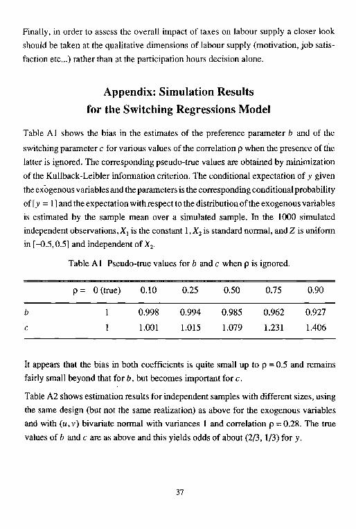
Appendix: Simulation Results

for the Switching Regressions Model

Table A I shows the bias in the estimates of the preference parameter b and of the

switching parameter c for various values of the correlation p when the presence of the

latter is ignored. The corresponding pseudo-true values are obtained by minimization

of the Kullback-Leibler information critelion. The conditional expectation of y given

the exogenous variables and the parameters is the corresponding conditional probability

of [y =1] and the expectation with respect to the distribution ofthe exogenous variables

is estimated by the sample mean over a simulated sample. In the 1000 simulated

independent observations, Xl is the constant 1, X2 is standard normal, and Z is uniform

in [-0.5,0.5] and independent of X2•

Table A 1 Pseudo-true values for b and c when p is ignored.

b

c

p = 0 (true) 0.10

0.998

1.001

0.25

0.994

1.015

0.50

0.985

1.079

0.75

0.962

1.231

0.90

0.927

1.406

It appears that the bias in both coefficients is quite small up to p =0.5 and remains

fairly small beyond that for b, but becomes important for c.

Table A2 shows estimation results for independent samples with different sizes, using

the same design (but not the same realization) as above for the exogenous variables

and with (u, v) bivariate normal with variances 1 and correlation p =0.28. The true

values of b and c are as above and this yields odds of about (2/3, 1/3) for y.

37

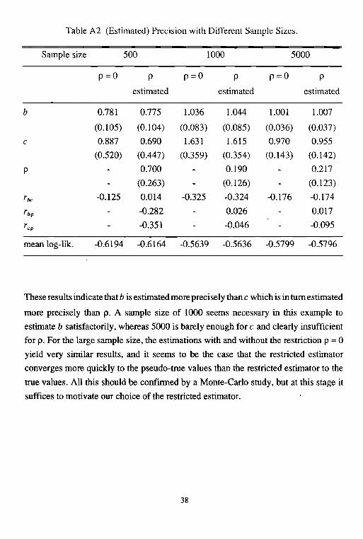
Table A2 (Estimated) Precision with Different Sample Sizes.

Sample size 500 1000 5000

p=o P p=o P p=o pestimated estimated estimated

b 0.781 0.775 1.036 1.044 1.001 1.007

(0.105) (0.104) (0.083) (0.085) (0.036) (0.037)

c 0.887 0.690 1.631 1.615 0.970 0.955

(0.520) (0.447) (0.359) (0.354) (0.143) (0.142)

P 0.700 0.190 0.217

(0.263) (0.126) (0.123)

roc -0.125 0.014 -0.325 -0.324 -0.176 -0.174

r bp -0.282 0.026 0.017

rep -0.351 -0.046 -0.095

mean log-Uk. -0.6194 -0.6164 -0.5639 -0.5636 -0.5799 -0.5796

These results indicate that b is estimated more precisely than c which is in tum estimated

more precisely than p. A sample size of 1000 seems necessary in this example to

estimate b satisfactorily, whereas 5000 is barely enough for c and clearly insufficient

for p. For the large sample size, the estimations with and without the restriction p =0

yield very similar results, and it seems to be the case that the restricted estimator

converges more quickly to the pseudo-true values than the restricted estimator to the

true values. All this should be confinued by a Monte-Carlo study, but at this stage it

suffices to motivate our choice of the restricted estimator.

38

ReferencesAtkinson, A.B. and J.E. Stiglitz (1980): Lectures in Public Economics. Maidenhead:

McGraw-Hill.

Blundell, R.W., F. Laisney and M. Lechner (1993): "Alternative Interpretations ofHours Information in an Econometric Model of Labour Supply", EmpiricalEconomics, 18,543-556.

Gabler, S., F. Laisney and M. Lechner (1990): "Seminonparametric Estimation ofBinary Choice Models With an Application to Labor-Force Participation",Journal ofBusiness and Economic Statistics, 11(1),61-80.

Hammond, P. (1989): "On the Impossibility of Perfect Capital Markets", EU! WorkingPapers in Economics No. 90/5.

Hausman, 1. (1985): "The Econometrics of Nonlinear Budget Sets", Econometrica, 53,1255-82.

Hausman, 1. and Wise D. (1978): "A Conditional Probit Model for Qualitative Choice:Discrete Decisions Recognizing Interdependence and Heterogenous Prefer­ences", Econometrica, 46,403-426.

Hujer, R. and R. Schnabel (1992): "Specification and Estimation of a Life-Cycle Modelof Female Labor Supply: A Microeconometric Analysis Using West-GermanPanel Data and Regional Indicators", working paper 338, Stb 3, UniversitatFrankfurt and Universitat Mannheim.

Kahneman D. and A. Tversky (1979): "Prospect Theory: An Analysis of Decisionsunder Risk", Econometrica, 47, 263-491.

Kiefer, N.M. (1979): "On the Value ofSample Separation Information", Econometrica,47,997-1003.

Laisney, E, M. Lechner and S. StrflSm (1991): "Lessons from specification tests for alabour supply model", Unjversitat Mannheim, discussion paper No. 416-90,forthcoming in Annales d' Economie et de Statistique, 21/22.

Laisney, F., M. Lechner,A. Van Soestand G. Wagenhals (1993): "A Life Cycle LabourSupply Model with with Taxes Estimated on German Panel Data: The Case ofParallel Preferences", The Economic and Social Review, 24, 335-368.

Lewis, A. (1982): The Psychology ofTaxation. Oxford: Martin Robertson.

Nakamura, A. and M. Nakamura (1981): "A Comparison of the Labor Force Behaviorof Married Women in the United States and Canada, with Special Attention tothe Impact of Income Taxes", Econometrica, 49,451-489.

Rosen, H.S. (1976a): "Taxes in a Labor Supply Model with 10int Wage-HoursDetermination", Econometrica, 44, 485 - 507.

Rosen, H.S. (1976b): "Tax Illusion and the Labor Supply Model of Married Women",Review ofEconomics and Statistics, 58, 167 -180.

Wahlund R. (1987): "Does Lowering the Marginal Tax Rates Matter?" ,paperpresentedat the 12th Annual Colloquium of the rAREP, the International Association forResearch on Economic Psychology, Arhus, September 25-28 1987.

39