Diurnal variation of turbulence-related quantities in Lake Garda

This article was downloaded by: [University Library Utrecht], [Lisa Hahn-Woernle]On: 18 December 2014, At: 07:40Publisher: Taylor & FrancisInforma Ltd Registered in England and Wales Registered Number: 1072954 Registeredoffice: Mortimer House, 37-41 Mortimer Street, London W1T 3JH, UK

Click for updates

Advances in Oceanography andLimnologyPublication details, including instructions for authors andsubscription information:http://www.tandfonline.com/loi/taol20

Diurnal variation of turbulence-relatedquantities in Lake GardaW.K. Lenstraa, L. Hahn-Woernlea, E. Mattab, M. Brescianib, C.Giardinob, N. Salmasoc, M. Musantib, G. Filab, R. Uittenbogaardd,M. Gensebergerd, H.J. van der Woerde & H.A. Dijkstraa

a Institute for Marine and Atmospheric Research Utrecht, Centerfor Extreme Matter and Emergent Phenomena, Utrecht University,The Netherlandsb Italian National Research Council – Institute for theElectromagnetic Sensing of the Environment, Via Bassini 15, 20133Milano, Italyc Sustainable Agro-ecosystems and Bioresources Department,IASMA Research and Innovation Centre, Istituto Agrario de S.Michele all’Adige – Fondazione E. Mach, Via E. Mach1, 38010, S.Michele all’Adige, Trento, Italyd Deltares, P.O. Box 177, 2600 MH, Delft, The Netherlandse Institute for Environmental Studies (IVM), De Boelelaan 1085,1081 HV Amsterdam, The NetherlandsPublished online: 04 Dec 2014.

To cite this article: W.K. Lenstra, L. Hahn-Woernle, E. Matta, M. Bresciani, C. Giardino, N.Salmaso, M. Musanti, G. Fila, R. Uittenbogaard, M. Genseberger, H.J. van der Woerd & H.A. Dijkstra(2014) Diurnal variation of turbulence-related quantities in Lake Garda, Advances in Oceanographyand Limnology, 5:2, 184-203, DOI: 10.1080/19475721.2014.971870

To link to this article: http://dx.doi.org/10.1080/19475721.2014.971870

PLEASE SCROLL DOWN FOR ARTICLE

Taylor & Francis makes every effort to ensure the accuracy of all the information (the“Content”) contained in the publications on our platform. However, Taylor & Francis,our agents, and our licensors make no representations or warranties whatsoever as tothe accuracy, completeness, or suitability for any purpose of the Content. Any opinionsand views expressed in this publication are the opinions and views of the authors,and are not the views of or endorsed by Taylor & Francis. The accuracy of the Content

should not be relied upon and should be independently verified with primary sourcesof information. Taylor and Francis shall not be liable for any losses, actions, claims,proceedings, demands, costs, expenses, damages, and other liabilities whatsoever orhowsoever caused arising directly or indirectly in connection with, in relation to or arisingout of the use of the Content.

This article may be used for research, teaching, and private study purposes. Anysubstantial or systematic reproduction, redistribution, reselling, loan, sub-licensing,systematic supply, or distribution in any form to anyone is expressly forbidden. Terms &Conditions of access and use can be found at http://www.tandfonline.com/page/terms-and-conditions

Dow

nloa

ded

by [

Uni

vers

ity L

ibra

ry U

trec

ht],

[L

isa

Hah

n-W

oern

le]

at 0

7:40

18

Dec

embe

r 20

14

Diurnal variation of turbulence-related quantities in Lake Garda

W.K. Lenstraa, L. Hahn-Woernlea*, E. Mattab, M. Brescianib, C. Giardinob, N. Salmasoc,

M. Musantib, G. Filab, R. Uittenbogaardd, M. Gensebergerd, H.J. van der Woerde and

H.A. Dijkstraa

aInstitute for Marine and Atmospheric Research Utrecht, Center for Extreme Matter and EmergentPhenomena, Utrecht University, The Netherlands; bItalian National Research Council � Institute

for the Electromagnetic Sensing of the Environment, Via Bassini 15, 20133 Milano, Italy;cSustainable Agro-ecosystems and Bioresources Department, IASMA Research and InnovationCentre, Istituto Agrario de S. Michele all’Adige � Fondazione E. Mach, Via E. Mach1, 38010,S. Michele all’Adige, Trento, Italy; dDeltares, P.O. Box 177, 2600 MH, Delft, The Netherlands;

eInstitute for Environmental Studies (IVM), De Boelelaan 1085, 1081 HV Amsterdam,The Netherlands

(Received 3 September 2014; accepted 29 September 2014)

To determine diurnal variations in the physical and biological state of Lake Garda inearly spring, high-resolution measurements were made of the vertical distribution oftemperature and fluorescence in the upper 100 meters during 5�7 March 2014. In thispaper, the results of these measurements are presented and a preliminary analysis thatfocuses on the connection between the vertical mixing coefficient KT and the chloro-phyll-a (chl-a) concentration is given. From these first direct measurements of turbu-lence-related quantities in Lake Garda, it is found that mixed-layer values of KT

decrease, while surface chl-a concentrations increase, over the day. Variations in KT

can be connected to the changes in the surface wind stress, while variations in chl-aare negatively correlated with the amplitude of KT . In addition, satellite observationsof the surface chl-a concentration are analysed to test their use for the calibration ofthe fluorescence measurements and also for their potential utility in remotely deter-mining vertical mixing in the upper layers of the lake.

Keywords: turbulence; stratification; microstructure profiler; plankton; chlorophyll-a;remote sensing; Lake Garda

1. Introduction

Lake Garda (45�400 N, 10�410 E) is a deep lake with a mean depth of 133 m, a maximum

depth of 350 m and a total volume of 49 million m3. With a surface area of 368 km2, it is

the largest fresh water lake in Italy. The concentration of chlorophyll-a (chl-a) in Lake

Garda ranges from 0.5 to 12 mg L�1, which is relatively low, and Lake Garda is classified

as an oligo-mesotrophic basin [1].

In lakes at temperate latitudes the plankton community evolves in an annually recur-

ring pattern [2], with the abrupt onset of phytoplankton growth in spring as a starting

point. The timing of the onset of the phytoplankton growth is controlled predominantly

by abiotic factors such as vertical mixing and variations in solar radiation [3]. In deep

lakes such as Lake Garda, interannual variations in the onset dominantly result from

changes in vertical mixing rather than solar variations and temperature [4].

*Corresponding author. Email: [email protected]

� 2014 Taylor & Francis

Advances in Oceanography and Limnology, 2014

Vol. 5, No. 2, 184�203, http://dx.doi.org/10.1080/19475721.2014.971870

Dow

nloa

ded

by [

Uni

vers

ity L

ibra

ry U

trec

ht],

[L

isa

Hah

n-W

oern

le]

at 0

7:40

18

Dec

embe

r 20

14

It was shown that external factors, such as winter air temperature, spring lake temper-

ature and the extent of surface nutrient enrichment, had significant effects on the phyto-

plankton distributions in Lake Garda over the period 1990�2003 [5]. For example in the

years 1991, 1999 and 2000, the whole water column was completely turned over as a con-

sequence of the harsh winters. These turnovers brought nutrients to the surface layers,

which in turn affected the growth of individual phytoplankton groups; their peaks

appeared at different times as well as at (mainly) higher concentrations than in other

years. Recently, limnological measurements and winter air temperature records have

been connected to the temporal variations of large scale atmospheric patterns, in particu-

lar the East Atlantic pattern and the Eastern Mediterranean pattern [6,7].

Climate change is unequivocally connected to an increase in surface temperature over

lakes in Western Europe, including Lake Garda. Increased temperatures will affect upper

lake temperatures and thermal stratification and hence are expected to change mixing

conditions. Climate warming may induce a shift in the timing and onset of the growth of

phytoplankton and hence strongly affect food-web interactions with zooplankton and fish

[8]. It is therefore important to understand the detailed causal chain between climate

change, changes in vertical mixing and the timing and extent of phytoplankton growth.

Although much has been inferred from the effects of the vertical mixing in Lake Garda,

direct measurements that can be used to determine the turbulence-related quantities are

lacking so far.

The objective of the present study was to gain a first insight into the turbulence-related

quantities of Lake Garda in early spring as well as into the sensitivity of the chl-a concen-

tration to diurnal changes in these quantities. We present preliminary results of the first

high-resolution measurements of the vertical temperature distribution (done with Self

Contained Autonomous Microstructure Profiles � SCAMP) in the upper 100 m of Lake

Garda. Based on these high-resolution measurements, profiles of the vertical mixing coef-

ficient KT as well as other turbulence-related quantities were determined. Measurements

of the vertical fluorescence distribution were calibrated with chl-a concentrations of water

samples to derive chl-a concentration profiles. Combining the chl-a measurements with

the KT data, the hypothesis of the negative effect of vertical mixing on phytoplankton

growth due to transport out of the photic zone is investigated. Finally, remote sensing

data (MODIS AQUA) of surface chl-a concentrations were compared with in situ concen-

trations to analyse the correspondence between the different measurement techniques and

the impact of spatial variance. This very preliminary picture of in situ and remote sensing

data will hopefully stimulate further research on the influence of the diurnal and seasonal

variations in turbulent mixing on the growth of phytoplankton at Lake Garda.

2. Data and methods

2.1. SCAMP measurements

The SCAMP is a free-falling instrument that measures the vertical temperature profile at a

frequency of 100 Hz down to a maximum depth of 100 m. The vertical temperature pro-

file is measured with two fast response thermistors and one accurate thermistor. The fast

sensors have a precision of 0:05�C, the more accurate thermistor measures with a preci-

sion of 0:02�C. The depth is measured with a pressure sensor with a precision of 0.5%

[9]. Based on the depth measurements, the free-fall velocity of the SCAMP is calculated

(� 0:1ms�1). The high sampling frequency results in a spatial resolution of » 1 mm,

which is needed to characterise the small-scale turbulent motions. At the top end of the

Advances in Oceanography and Limnology 185

Dow

nloa

ded

by [

Uni

vers

ity L

ibra

ry U

trec

ht],

[L

isa

Hah

n-W

oern

le]

at 0

7:40

18

Dec

embe

r 20

14

SCAMP a Photo-synthetically Active Radiation (PAR) sensor is installed. The PAR pro-

files are used to define the photic depth for which the PAR signal decreases to 0.01% of

the incoming intensity (� 30�45 m) and for the depth above which 90% of the backscat-

tered irradiance originates, z90 (� 14 m). The latter is used for comparison with satellite

surface chl-a concentration [10,11].

Above the thermistors there is an inlet where water can flow through the SCAMP

from which the fluorescence is measured. The fluorescence signal is based on the photo-

system properties of the chl-a cells and measurements are given in volts. It is well known

that the relation to chl-a cells is not linear and optical properties may change over depth.

At the surface phytoplankton cells commonly adapt to the high light availability, also

known as non-photochemical quenching [12]. Therefore surface values of the fluores-

cence measurements are excluded from the analysis.

The conversion from volts to chl-a concentration needs to be determined from in situ

or satellite measurements of the chl-a concentration. The determination of the conversion

factor is described in more detail in Appendix A.

The SCAMP is provided with MATLAB�software, with which the measured profiles

are preprocessed before analysis. First, a sharpening, smoothening, trimming and second-

order Butterworth brick-wall filtering are performed [13]. Next, the measured profiles are

depth-binned; here, one-meter bins are chosen because of a trade-off between having suf-

ficient vertical resolution and good statistical robustness. Finally, the arithmetic mean of

each bin is calculated to determine the temperature profiles for further analysis. In the fol-

lowing, these profiles will be referred to as the processed data.

More detailed information about the SCAMP can be found on the webpage of PME

(http://www.pme.com/).

2.2. Determination of turbulence-related quantities

Assuming that dependent quantities are horizontally uniform and that the time mean of the

vertical velocity is zero (w = 0), the temperature variance equation can be written as [14]

@

@tðT 0 Þ2 ¼ �2ðw 0 T 0 Þ @T

@z� x; (1)

where the depth z is taken positive in the downward direction, the bar indicates the time

mean and the prime the deviation from the time mean. In Equation (1), the first term on

the right hand side is the production of thermal variance by the vertical heat flux. The sec-

ond term is the dissipation of thermal variance by thermal diffusion x, which is given by

x ¼ 6k@T 0

@z

� �2

; (2)

where k is the (molecular) thermal diffusivity. Assuming that the production and dissipa-

tion terms approximately balance [15] and using the following first-order closure for the

turbulent heat flux:

w 0T 0 ¼ �KT

@T

@z; (3)

186 W.K. Lenstra et al.

Dow

nloa

ded

by [

Uni

vers

ity L

ibra

ry U

trec

ht],

[L

isa

Hah

n-W

oern

le]

at 0

7:40

18

Dec

embe

r 20

14

the vertical mixing coefficient KT is found from

KT ¼ x

2

@T

@z

� ��2

: (4)

The dissipation of turbulent kinetic energy e is determined by considering processes at

the Batchelor length scale lB, at which the advection and diffusion of heat approximately

balance. The relation between e and lB is given by [15]

lB ¼ nk2

e

� �1=4

; (5)

where n is the (molecular) kinematic viscosity. The Batchelor wave number kB is the

inverse of the Batchelor length scale (kB ¼ 1=lB) and can be estimated by fitting a Batche-

lor spectrum to the Fourier transform of the temperature gradient measurements. We used

the maximum likelihood method developed by Ruddick et al. [15], which is further

explained in Appendix B.

When kB is determined, e is found for each segment from

e ¼ ð2pkBmaxÞ4nk2: (6)

Here n is the arithmetic mean of the molecular kinematic viscosity in the segment and

kBmax is the optimal value of the Batchelor wave number. From early experimental work

[16,17] it was concluded that values for edetermined indirectly through Batchelor fitting

agree within a factor of two with values for e determined from the vertical shear fluctua-

tions of the flow.

According to Osborn�Cox theory [14], the relationship between the vertical mixing

coefficient KT , the turbulent kinetic energy dissipation e, and the squared Brunt V€ais€al€afrequency (N 2 s�2) is expected to be

KT ¼ GeN2

; (7)

where G � 0:2 is the so-called mixing efficiency. Formally, this relation only holds under

very idealised circumstances [18].

In the open ocean, the depth of the mixed layer (ML) is usually determined by the

depth at which the temperature difference with respect to the surface is 0.5�C [19]. As

will be shown below, the water temperature measured at Lake Garda only varies verti-

cally by a maximum of 0.4�C. To take this small temperature gradient into account, we

defined the ML depth as the depth where the temperature deviated by 0.11�C from the

average temperature over the upper 10 m. The averaging over the first 10 m was done to

avoid a strong influence of relatively high temperatures at the surface. The value of

0.11�C was chosen so that the ML depth results are in good agreement with the depth at

which the maximum temperature gradient occurs.

2.3. Additional data

Daily water samples at different depths (surface, 15, 30 and 45 m) were collected in Van

Dorne bottles for subsequent laboratory analyses to determine, amongst other things, the

Advances in Oceanography and Limnology 187

Dow

nloa

ded

by [

Uni

vers

ity L

ibra

ry U

trec

ht],

[L

isa

Hah

n-W

oern

le]

at 0

7:40

18

Dec

embe

r 20

14

chl-a and soluble reactive phosphorus (SRP) concentrations. For the chl-a concentration,

acetone (90%) extraction according to Lorenzen [20] was used, and for the SRP concen-

tration, spectrophotometric determination according to the American Public Health Asso-

ciation [21] was used.

MODIS AQUA (MYD021KM product) Level 1B data were used to determine surface

chl-a concentrations. Radiance products were corrected for the atmospheric effect with

the 6SV1 code (Second Simulation of a Satellite Signal in the Solar Spectrum, Vector,

version 1) [22].

The spectral inversion procedure BOMBER [23], implementing a four-component

bio-optical model, was used to estimate chl-a from MODIS-derived remote sensing

reflectance data (Rrs). The bio-optical model parameterisation relies on a comprehensive

dataset of concentrations and optical properties measured in Lake Garda in recent years

[24,25].

Due to incomplete data sets from the local weather stations, meteorological data were

taken from COSMO-2 model data (MeteoSwiss, http://www.cosmo-model.org/content/

tasks/operational/meteoSwiss/). The data include wind speed data at 10 m, the net surface

heat flux, air temperature, relative humidity and air pressure. The data are given with a

high spatial (2.2 km) and temporal (1 hour) resolution and for each variable the mean

over the southern part of the lake (45.4785�45.6181�N, 10.5703�10.6575�E) is used.

The wind stress amplitude t0 on the water surface is calculated with the help of

t0 ¼ raCDU210; (8)

where CD is the wind-drag coefficient (here taken as a constant, CD ¼ 1:310�3), ra is the

density of air, and U10 is the wind speed at a height of 10 m.

3. Results

3.1. Measurement locations

The measurements in Lake Garda were carried out at four stations over three days from 5

to 7 March 2014. In Figure 1, a map of the southern part of Lake Garda is shown where

the dots indicate the locations of the stations. In Table 1, the coordinates of the stations

and the number of SCAMP vertical profiles measured at each station are listed. During

rough weather it was more difficult to obtain data of good quality and fewer profiles were

obtained. At the two southern stations (red and green) previous measurements of the opti-

cal properties of the water had been done which motivated their choice. We added two

northern stations (blue and black) to determine any geographical variations. The SCAMP

measurements were split into morning sets (before 13:00) and afternoon sets (after

13:00). After sampling all four stations during one set, we spent the whole day of 7 March

at the green station to capture the diurnal variations at one location.

3.2. Meteorological forcing

Figure 2(a) shows the surface wind stress calculated from the COSMO-2 wind speed with

Equation (8). In general, the wind speed � and thereby the wind stress � was relatively

high in the morning, while it decreased in the afternoon. The whole day of 6 March was

characterised by higher wind speeds in comparison to the other two days (5 and 7 March).

The resulting surface wind stress ranged from 0.1£ 10�3 to 0.26 N m�2. The largest peak

188 W.K. Lenstra et al.

Dow

nloa

ded

by [

Uni

vers

ity L

ibra

ry U

trec

ht],

[L

isa

Hah

n-W

oern

le]

at 0

7:40

18

Dec

embe

r 20

14

in wind stress occurred during the night of 6 March. Smaller peaks occured around noon

of 5 March and in the morning of 7 March.

Contributions to the surface heat balance from the COSMO-2 model output are plotted in

Figure 2(b). The net heat flux negative for heat entering the water) is mainly controlled by

the net shortwave heat flux. The net longwave heat flux and latent heat flux only provide a

substantial contribution to the total heat flux during night. The sensible heat flux is negligibly

small. The daily integrated heat fluxes per day were �2.5 MJ/m2 (5 March), +1.4 MJ/m2

(6 March) and�1.6 MJ/m2 (7 March). The positive value on 6 March means that the lake was

cooling during that day while it was heating during the other two days. From Figure 2(b), one

can see that the cooling mainly happened in the night from 5 to 6 March.

Figure 1. Stations at Lake Garda (colored dots) where SCAMP profiles were measured and watersamples were taken during the period 5�7 March 2014. Contours give the depth in meters. The pre-cise locations and details concerning the number of profiles can be found in Table 1.

Table 1. Detailed information about the SCAMP measurement stations: the location in LakeGarda, the date and time span (UTC+02:00) of measurements, the maximum depth range of themeasurements and the number of profiles measured.

Station Location Date and time Depth range No. of profiles

45.544�N 5 Mar 2014

Blue 10.618�E 09:50�12:20 2�100 m 6

45.563�N 5 Mar 2014

Black 10.621�E 15:05�18:00 2�99 m 6

45.494�N 6 Mar 2014

Red 10.567�E 14:30�16:40 2�47 m 8

6 Mar 2014

10:40�12:50 2�73 m 5

45.524�N 7 Mar 2014

Green 10.602�E 10:50�12:30 2�76 m 5

7 Mar 2014

13:50�16:50 2�75 m 8

Advances in Oceanography and Limnology 189

Dow

nloa

ded

by [

Uni

vers

ity L

ibra

ry U

trec

ht],

[L

isa

Hah

n-W

oern

le]

at 0

7:40

18

Dec

embe

r 20

14

3.3. Mean vertical temperature profiles

Based on the SCAMP measurements, the mean processed temperature profiles are plotted

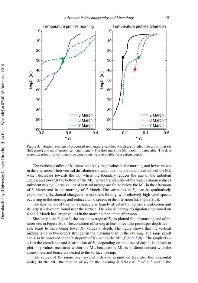
in Figure 3 for the morning set (left) and the afternoon set (right). During the day, the pro-

files show an increase in stratification because of surface heating and calmer weather con-

ditions in the afternoon.

On 5 March, the morning temperature profile shows an almost homogeneous upper

layer with a small upward sloping profile, while the afternoon profile shows a small tem-

perature step at about 25 m depth. On 6 and 7 March, the morning and afternoon tempera-

ture profiles have a similar shape with an increased surface temperature in the afternoon.

The strong cooling in the night from 5 to 6 March leads to a weak stratification in the

morning of 6 March. The maximum measurement depth for the red station on 6 March is

limited because the station is located in a relatively shallow part of Lake Garda.

Over the three days, a stratification build-up is seen in the morning profiles with a

temperature step of about 0.15�C appearing near 30 m depth at 7 March. The same also

holds for the afternoon profiles, which show mainly a deepening of the warm surface

water and the development of a clear ML.

3.4. Turbulence-related quantities

Figure 4 shows the vertical profiles of (a) KT , (b) x and (c) e, which were derived from the

temperature profiles according to Equations (4), (2) and (6), respectively. Missing data

points (white areas) occur due to insufficient quality of the Batchelor fit as discussed in

Appendix B.

Figure 2. Meteorological conditions during the Lake Garda measurements based on the COSMO-2model (data obtained from MeteoSwiss) plotted over the three days (0:00 meaning midnight). (a)Wind stress as determined from Equation (8); (b) terms in the surface heat balance (negative whenheat enters the lake) with net surface heat flux (black), net shortwave heat flux (blue), net longwaveheat flux (red), sensible heat flux (magenta), and latent heat flux (green).

190 W.K. Lenstra et al.

Dow

nloa

ded

by [

Uni

vers

ity L

ibra

ry U

trec

ht],

[L

isa

Hah

n-W

oern

le]

at 0

7:40

18

Dec

embe

r 20

14

The vertical profiles of KT show relatively large values in the morning and lower values

in the afternoon. Their vertical distribution shows a maximum around the middle of the ML

which decreases towards the top, where the boundary reduces the size of the turbulent

eddies, and towards the bottom of the ML, where the stability of the water column reduces

turbulent mixing. Large values of vertical mixing are found below the ML in the afternoon

of 5 March and in the morning of 7 March. The variations in KT can be qualitatively

explained by the diurnal changes of wind stress forcing, with relatively high wind speeds

occurring in the morning and reduced wind speeds in the afternoon (cf. Figure 2(a)).

The dissipation of thermal variance x is largely affected by thermal stratification and

its largest values are found near the surface. The kinetic energy dissipation e measured on

6 and 7 March has larger values in the morning than in the afternoon.

Similarly as in Figure 3, the station average of KT is plotted for all morning and after-

noon sets in Figure 5(a). The condition of having at least three data points per depth avail-

able leads to there being fewer KT values at depth. The figure shows that the vertical

mixing is up to two orders stronger in the morning than in the evening. The same result

can also be observed in the histogram of KT within the ML (Figure 5(b)). The graph visu-

alises the abundance and distribution of KT depending on the time of day. It is chosen to

plot only values measured within the ML because the ML is in direct contact with the

atmosphere and hence connected to the surface forcing.

The values of KT range over several orders of magnitude (see also the horizontal

scale). In the ML, the median of KT in the morning is 5:93£10�4 m2 s�1 and in the

Figure 3. Station average of processed temperature profiles, which are divided into a morning set(left panel) and an afternoon set (right panel). The dots mark the ML depth, if detectable. The datawere discarded if fewer than three data points were available for a certain depth.

Advances in Oceanography and Limnology 191

Dow

nloa

ded

by [

Uni

vers

ity L

ibra

ry U

trec

ht],

[L

isa

Hah

n-W

oern

le]

at 0

7:40

18

Dec

embe

r 20

14

Figure 4. Vertical, depth binned profiles of the turbulence-related quantities KT (a), x (b) and e(c) derived from the SCAMP temperature profiles measured during 5�7 March. Vertical black linesseparate the different days, red lines indicate the difference between morning and afternoon. Smallhorizontal black bars indicate the depth of the ML. The colors on the x-axis indicates the stationwhere the measurements were done, as shown in Figure 1. The small black dots represent the maxi-mum depth of each SCAMP measurement.

192 W.K. Lenstra et al.

Dow

nloa

ded

by [

Uni

vers

ity L

ibra

ry U

trec

ht],

[L

isa

Hah

n-W

oern

le]

at 0

7:40

18

Dec

embe

r 20

14

afternoon it is 3:11£10�5 m2 s�1. The median of x in the morning is 1:49£10�8 K2 s�1

and in the afternoon it is 6:86£10�10 K2 s�1. The median of e in the morning is

9:16£10�8 m2 s�3 and in the afternoon it is 3:29£10�10 m2 s�3.

In order to provide a preliminary test of Osborn�Cox theory as given in Equation (7),

the relation of logðKT Þ to logðe=N 2Þ and to logðNÞ is plotted in Figures 6(a) and 6(b),

respectively. The results in Figure 6(a) indicate that the value of G is not independent of

e=N 2. The relation between KT and N in Figure 6(b) shows the effect of the background

stratification on the vertical mixing and appears to agree more closely with theory, with

the data spreading around the theoretical slope of �2.

Considering also previous studies [26,27], our measurements are likely to lie in

a turbulence regime for which Osborn�Cox theory is too idealised, but a more quantita-

tive analysis (and more SCAMP measurements) are necessary to be conclusive here.

3.5. In situ determined chlorophyll-a

Based on the calibrated fluorescence profiles, the measured chl-a concentration (in mg L�1)

is shown in Figure 7. Most profiles show a clear sign of the ML in their chl-a distribution

Figure 5. Diurnal variation of KT in the ML. (a) Mean profiles of KT in the morning (left) andafternoon (right). (b) Histogram of KT values; the dark green bars indicate that morning values(blue) are plotted behind afternoon values (green).

Advances in Oceanography and Limnology 193

Dow

nloa

ded

by [

Uni

vers

ity L

ibra

ry U

trec

ht],

[L

isa

Hah

n-W

oern

le]

at 0

7:40

18

Dec

embe

r 20

14

with a strong gradient in the chl-a concentration at the ML depth. Only in the morning of

5 March was the stratification still weak and mixing to greater depths possible. Concentra-

tions within the ML are rather homogeneous (note that the first 5�10 m at the surface are

excluded from the analysis due to the possibility of non-photochemical quenching).

For most sets the chl-a concentration increases with time, but the strength of this trend

varies strongly; while both sets on 7 March show an increase in chl-a, the morning set of 5

March and the afternoon set of 6 March show no trend. A possible explanation of this

behavior could be the deep ML. Deep vertical mixing spreads the phytoplankton cells

into regions below the photic layer where growth does not occur due to the lack of PAR.

This could lead to the inhomogeneous distribution of chl-a. A trend towards a higher con-

centrations at the surface can only be initiated by the shallowing of the ML [28,29]. The

Figure 6. Relation of logðKT Þ to (a) logðe=N 2Þ and (b) logðNÞ. The lines in both panels would bethe relation according to Osborn�Cox theory.

194 W.K. Lenstra et al.

Dow

nloa

ded

by [

Uni

vers

ity L

ibra

ry U

trec

ht],

[L

isa

Hah

n-W

oern

le]

at 0

7:40

18

Dec

embe

r 20

14

net shortwave heat flux (blue line in Figure 2(b)) seems to increase over the three days

too, which can lead to increased phytoplankton growth and a decrease of the ML depth.

Both processes enhance the chl-a concentration.

Another interesting feature is the difference in the two morning sets at the green sta-

tion: on 6 March the chl-a concentration is high and spreads deep while on 7 March con-

centrations are considerably lower and reach 10 m less deep. The difference in the depth

of the spread can be explained by the lower ML depth on 7 March in comparison to 6

March. The difference in the concentration could again be explained by the depth of the

ML. Another explanation could be ‘turbulence avoidance’ by zooplankton. Under normal

conditions, zooplankton migrate to the surface at night to eat phytoplankton. In [30], tur-

bulence avoidance is described as the migration of zooplankton to deeper layer to avoid

turbulent transport at the surface. Wind-stress amplitudes of 0.0398 to 0.1593 N m�2 are

described as sufficient to prevent turbulent sensitive species entering the surface layer.

Wind-stress values above this critical value are found at 6 March during the night

(Figure 2(a)). Proof of the absence of zooplankton could not be provided because zoo-

plankton concentrations were not measured.

To address our main hypothesis regarding the effect of vertical mixing on the chl-a

concentration, the average values within the ML of the chl-a concentration and of KT are

plotted against each other in Figure 8. The chl-a concentration is negatively correlated

with the value of the vertical mixing coefficient. This result supports the hypothesis of

reduced growth under higher vertical mixing conditions due to light limitation. Regarding

the outliers in Figure 7, it can be seen that the morning set of 5 March fits into the case of

high vertical mixing and low chl-a concentrations while the morning set of 6 March

clearly deviates from this.

Another possible explanation for the negative correlation between chl-a concentration

and vertical mixing could be that strong mixing brings most of the phytoplankton cells in

contact with the surface. At the surface, the high light intensity will lead to non-photo-

chemical quenching, which weakens the fluorescence signal of these cells even when

they are mixed into deeper depths again. Weak mixing, however, keeps these affected

cells mainly at the surface and non-photochemical quenching has less influence on the

Figure 7. Depth binned profiles of the chlorophyll-a concentration as measured with the SCAMPduring 5�7 March. For further description, see the caption to Figure 4.

Advances in Oceanography and Limnology 195

Dow

nloa

ded

by [

Uni

vers

ity L

ibra

ry U

trec

ht],

[L

isa

Hah

n-W

oern

le]

at 0

7:40

18

Dec

embe

r 20

14

fluorescence signal below the surface, which means that the strength of the fluorescence

signal is not influenced by the quenching.

3.6. Satellite determined chlorophyll-a

Figure 9 shows the daily maps of chl-a retrieved concentrations measured by MODIS

AQUA after applying BOMBER [23] during 5�7 March; a comparison with chl-a mea-

sured in the laboratory shows an RSME (root mean square error) of 30%. The chl-a con-

centration shows a slight latitudinal trend along the four stations with decreasing

concentrations northwards. This is a very interesting feature, which could not be captured

in the SCAMP measurements since diurnal variations are too dominant and the time

Figure 8. Correlation between KT and chl-a in the ML.

Figure 9. The MODIS AQUA-retrieved chl-a concentrations on 5, 6 and 7 March 2014. Circlesindicate the measurement stations during the corresponding days.

196 W.K. Lenstra et al.

Dow

nloa

ded

by [

Uni

vers

ity L

ibra

ry U

trec

ht],

[L

isa

Hah

n-W

oern

le]

at 0

7:40

18

Dec

embe

r 20

14

series is too short. On 6 March, chl-a patterns are more patchy than those at the other

days, which could have two possible explanations: the high wind-forcing during that day

(Figure 2(a)), and the location of Lake Garda within the MODIS scene (MODIS has a

viewing swath width of 2.3 km). On 6 March, the lake is located close to the swath edge

where image data are usually nosier due to geometric distortion [31].

In Figure 10, the surface chl-a concentration based on SCAMP data and on MODIS

AQUA data is plotted. SCAMP values are calculated as the mean concentration of chl-a

above z90. They show that concentrations increase steadily during the day by about 50%

of their initial value except for 6 March. The MODIS AQUA data of the corresponding

time and location are shown to be of the same order of magnitude as the SCAMP data,

but with a discrepancy of up to 40%. Taking into account the fast changes in chl-a con-

centration, the 30% RMSE of the MODIS AQUA data and the uncertainty in the calibra-

tion of the SCAMP fluorometer, the two measurement methods seem to be in reasonable

agreement.

In Table 2, an overview of the data based on water samples, SCAMP profiles and

remote sensing is given. From these samples the concentrations of chl-a (column 4) and

of soluble reactive phosphorous SRP (last column) are determined. Column 5 gives the

comparable SCAMP chl-a concentrations, which are for the surface values the mean over

2�5 m depth and placed in parentheses owing to the effect of non-photochemical quench-

ing. The comparable value at depth is the 5 m mean around the corresonding sample

depth to take the uncertainty in the depth of the bottles into account. At the red station the

SCAMP measurements were not deep enough when the samples were taken. Columns 6

and 7 give the surface chl-a concentration as discussed above (and shown in Figure 9).

Because MODIS AQUA data is available only once per day, there is only one SCAMP

surface value per day and per location to compare this data with. In general, a reasonable

Figure 10. Mean surface chl-a concentration measured with the SCAMP. Values are averaged overz90. For clarity, the data are divided into three different days. Upwards pointing triangles indicatethe MODIS-AQUA chl-a measurements at the corresponding times.

Advances in Oceanography and Limnology 197

Dow

nloa

ded

by [

Uni

vers

ity L

ibra

ry U

trec

ht],

[L

isa

Hah

n-W

oern

le]

at 0

7:40

18

Dec

embe

r 20

14

correlation between the different chl-a measurements is found, especially between

MODIS AQUA and bottle samples at the surface and between SCAMP and bottle sam-

ples at depth. The latter may be influenced by the calibration of the SCAMP fluorescence

data to the bottle samples at depth (see Appendix A). The surface bottle sample of 6

March in the morning is exceptionally high. A comparison with the z90-mean (column 7)

and their compatibility with the MODIS AQUA data underlines the importance of the

optical properties involved in the measurement and analysis of the chl-a concentration. In

Lake Garda, SRP can become a limiting factor for phytoplankton growth, but generally

this is not the case in spring [6,7]. The bottle samples also suggest that the growth is not

nutrient limited, but the data is too sparse to draw firm conclusions.

4. Summary and discussion

We have presented a preliminary analysis of turbulence-related quantities and phyto-

plankton (chl-a) distributions of the upper 100 m of Lake Garda in early spring using

SCAMP data, water samples and MODIS AQUA satellite measurements. We found that

the stratification was building up over the three days of measurements and that diurnal

changes in the strength of the vertical mixing occurred and were mainly driven by the

change in wind stress. Furthermore, the vertical mixing was shown to be negatively corre-

lated to the strength of the background stratification.

The surface chl-a concentrations increased during the day and the diurnal variation of

the chl-a concentration (cf. Figure 7) appears to be sensitive to external factors. The

nature of these external factors can be very different, e.g. grazing and nutrient limitation,

and cannot be captured by the measurements done here. The correlation between the ver-

tical mixing coefficient and the chl-a concentration measured in the ML is clearly nega-

tive, which indicates that wind stress induced mixing is effectively limiting the

phytoplankton growth during early March. A comparison of the in situ and remote sens-

ing data showed that the uncertainty of the satellite data is still too high to use it for direct

Table 2. Measurements of chl-a and soluble reactive phosphorus (SRP) concentrations (all inmg L�1) for different depths and locations during 5�7 March in Lake Garda. Bold font measure-ment depths indicate measurements below the ML in the hypolimnion. The SCAMP surface valuesin column 5 are values of chl-a averaged over the first 2 to 5 m and the surface values of column 7are averaged over z90.

Date Station DepthSamplechl-a

SCAMPchl-a

MODISchl-a

SCAMPchl-a(z90Þ

SampleSRP

5 March blue surface 1.94 (0.92) 1.99 1.58 14.7

30 m 2.43 2.29 14.7

5 March black surface 1.26 (1.46) 1.79 � 6.3

45 m 1.34 1.47 10.5

6 March green surface 3.97 (1.24) 1.44 2.23 23.2

45 m 1.40 1.47 9.1

6 March red surface 2.44 (1.06) 2.23 � 7.7

45 m 2.04 � 10.5

7 March green surface � � 2.30 1.54 �15 m 2.60 2.25 19.0

30 m 2.25 2.47 7.7

198 W.K. Lenstra et al.

Dow

nloa

ded

by [

Uni

vers

ity L

ibra

ry U

trec

ht],

[L

isa

Hah

n-W

oern

le]

at 0

7:40

18

Dec

embe

r 20

14

calibration. However, the remote sensing data provide a valuable picture of the spatial

variability of surface chl-a concentrations in Lake Garda.

Although the data are sparse and the analysis very preliminary, the results presented

provide a good overview of the vertical distribution of turbulence-related quantities that

can be connected to surface forcing as well as to background stratification. The nature of

the negative correlation between KT and the chl-a concentration can be due to the mixing

of the phytoplankton cells at the lower boundary of the photic zone and beyond. Alterna-

tively, it can also be due to the distribution of cells affected by non-photochemical

quenching in the case of strong mixing. In the case of weak mixing, these cells mainly

remain at the surface and do not affect the fluorescence signal at greater depths.

The results here also suggest a number of improvements for further research. The

measurements are too sparse and spatially inhomogeneous for a quantitative connection

between surface forcing and turbulence-related quantities, such as were made, for exam-

ple, for the open ocean in [9]. For the analysis of this connection, we suggest measuring

the atmospheric forcing directly on the water at the location of the SCAMP measurements.

The analysis of the turbulence-related quantities with the SCAMP would also benefit from

a larger number of vertical profiles at each location to become statistically more robust.

The calibration of the fluorescence measurements to in situ bottle samples is a well-

known problem since the conversion from fluorescence to chl-a is not provided by a uni-

versal constant. Instead, it is sensitive to biochemical effects like non-photochemical

quenching. Especially measurements close to the surface are affected and fluorescence

data cannot be trusted. We therefore suggest taking bottle samples with higher vertical

resolution for better calibration of the fluorometer as well as more detailed biochemical

analysis. The latter should include the determination of zooplankton concentration such

that the zooplankton turbulence avoidance mechanism can be tested. Also, the determina-

tion of the nutrient composition and concentration will be of high relevance, particularly

during summer, at which time nutrient depletion in the surface water can lead to substan-

tial changes in the composition of the phytoplankton population. Such changes in the pop-

ulation and the growth environment may lead to a different correlation between the

vertical mixing coefficient KT and the chl-a concentration than the correlation found here.

Finally, we hope that the paper has illustrated the potential of the SCAMP for measur-

ing vertical mixing properties in deep lakes and that the results will stimulate further

experimental work on the connection between vertical mixing and phytoplankton distri-

butions in Lake Garda.

Acknowledgements

The authors are very grateful to M. Bartoli and M. Pinardi (University of Parma) for laboratoryanalysis and to I. Cazzaniga (CNR-IREA) for support in data processing.

Meteorological data have been provided by MeteoSwiss, the Swiss Federal Office of Meteorol-ogy and Climatology.

Special thanks go also to the work of the two anonymous reviewers who read our manuscript incritical detail and provided us with highly valuable input.

Funding

This work was funded by the NSO User Support Programme through the COLOURMIX project withfinancial support from the Netherlands Organization for Scientific Research (NWO) [grant numberALW-GO-AO/11-08]. This study was co-funded by GLaSS (7th Framework Programme) [project num-ber 313256]; and CLAM-PHYM (the Italian Space Agency) [contract number I/015/11/0].

Advances in Oceanography and Limnology 199

Dow

nloa

ded

by [

Uni

vers

ity L

ibra

ry U

trec

ht],

[L

isa

Hah

n-W

oern

le]

at 0

7:40

18

Dec

embe

r 20

14

References

[1] C. Giardino, V.E. Brando, A.G. Dekker, N. Str€ombeck, and G. Candiani, Assessment of waterquality in Lake Garda (Italy) using Hyperion, Remote Sens. Environ. 109 (2007),pp. 183�195.

[2] U. Sommer, Plankton Ecology � Succession in Plankton Communities, Springer, Berlin,1989.

[3] W. Bleiker and F. Schanz, Influence of environmental factors on the phytoplankton springbloom in Lake Z€urich, Aquat. Sci. 51 (1989), pp. 47�58.

[4] F. Peeters, D. Straile, A. Lorke, and D. Ollinger, Turbulent mixing and phytoplankton springbloom development in a deep lake, Limnol. Oceanogr. 52 (2007), pp. 286�298.

[5] N. Salmaso, Effects of climatic fluctuations and vertical mixing on the interannual trophicvariability of Lake Garda, Italy, Limnol. Oceanogr. 50 (2005), pp. 553�565.

[6] N. Salmaso, Influence of atmospheric modes of variability on a deep lake south of the Alps,Climate Res. 51 (2012), pp. 125�133.

[7] N. Salmaso, F. Buzzi, L. Cerasino, L. Garibaldi, B. Leoni, G. Morabito, M. Rogora, and M.Simona, Influence of atmospheric modes of variability on the limnological characteristics oflarge lakes south of the Alps: a new emerging paradigm, Hydrobiologia 731 (2013),pp. 31�48.

[8] M. Scheffer, D. Straile, E.H. van Nes, and H. Hosper, Climatic warming causes regime shiftsin lake food webs, Limnol. Oceanogr. 46 (2001), pp. 1780�1783.

[9] E. Jurado, H.J. van der Woerd, and H.A. Dijkstra, Microstructure measurements along aquasi-meridional transect in the northeastern Atlantic Ocean, J. Geophys. Res.�Oceans(1978�2012) 117 (2012), C04016. doi:10.1029/2011JC007137

[10] H.R. Gordon and D.K. Clark, Remote sensing optical properties of a stratified ocean: animproved interpretation, Appl. Optics 19 (1980), pp. 3428�3430.

[11] P.J. Werdell and S.W. Bailey, An improved in-situ bio-optical data set for ocean color algo-rithm development and satellite data product validation, Remote Sens. Environ. 98 (2005),pp. 12�140.

[12] P. Muller, X.P. Li, and K.K. Niyogi, Non-photochemical quenching. A response to excess lightenergy, Plant Physiol. 125 (2001), pp. 1558�1566.

[13] F.M. Fozdar, G.J. Parkar, and J. Imberger, Matching temperature and conductivity sensorresponse characteristics, J. Phys. Oceanogr. 15 (1985), pp. 1557�1569.

[14] T.R. Osborn and C.S. Cox, Oceanic fine structure, Geophys. & Astrophys. Fluid Dyn. 3(1972), pp. 321�345.

[15] B. Ruddick, A. Anis, and K. Thompson, Maximum likelihood spectral fitting: the Batchelorspectrum, J. Atmos. Ocean. Technol. 17 (2000), pp. 1541�1555.

[16] T.M. Dillon and D.R. Caldwell, The Batchelor spectrum and dissipation in the upper ocean, J.Geophys. Res.�Oceans (1978�2012) 85 (1980), pp. 1910�1916.

[17] N.S. Oakey, Determination of the rate of dissipation of turbulent energy from simultaneoustemperature and velocity shear microstructure measurements, J. Phys. Oceanogr. 12 (1982),pp. 256�271.

[18] B. Ruddick, D. Walsh, and N. Oakey, Variations in apparent mixing efficiency in the NorthAtlantic Central Water, J. Phys. Oceanogr. 27 (1997), pp. 2589�2605.

[19] S. Levitus, J.I. Antonov, T.P. Boyer, and C. Stephens, Warming of the world ocean, Science287 (2000), pp. 2225�2229.

[20] C.J. Lorenzen, Determination of chlorophyll and phaeo-pigments: spectrophotometric equa-tions, Limnol. Oceanogr. 12 (1967), pp. 343�346.

[21] APHA (American Public Health Association), AWWA (American Water Works Association),and WPCF (Water Pollution Control Federation),Standard methods for the examination ofwater and wastewater, American Public Health Association, Washington, DC, 1981.

[22] S.Y. Kotchenova, E.F. Vermote, R. Matarrese, F.J. Klemm Jr, Validation of a vector versionof the 6S radiative transfer code for atmospheric correction of satellite data. Part I: Path radi-ance, Appl. Optics 45 (2006), pp. 6762�6774. doi:10.1364/AO.45.006762

[23] C. Giardino, G. Candiani, M. Bresciani, Z. Lee, S. Gagliano, and M. Pepe, BOMBER: a toolfor estimating water quality and bottom properties from remote sensing images, Comput.Geosci. 45 (2012), pp. 313�318.

[24] M. Bresciani, R. Bolpagni, F. Braga, A. Oggioni, and C. Giardino, Retrospective assessmentof macrophytic communities in southern Lake Garda (Italy) from in situ and MIVIS

200 W.K. Lenstra et al.

Dow

nloa

ded

by [

Uni

vers

ity L

ibra

ry U

trec

ht],

[L

isa

Hah

n-W

oern

le]

at 0

7:40

18

Dec

embe

r 20

14

(Multispectral Infrared and Visible Imaging Spectrometer) data, J. Limnol. 71 (2012),pp. 180�190. doi:10.4081/jlimnol.2012.e19

[25] C. Giardino, G. Candiani, M. Bresciani, M. Bartoli, and L. Pellegrini, Multi-spectral IR andvisible imaging spectrometer (MIVIS) data to assess optical properties in shallow waters, in3rd EARSeL Workshop on Remote Sensing of the Coastal Zone, 7�9 June 2007, Bolzano,Italy.

[26] L.H. Shih, J.R. Koseff, G.N. Ivey, and J.H. Ferziger, Parameterization of turbulent fluxes andscales using homogeneous sheared stably stratified turbulence simulations, J. Fluid Mech.525 (2005), pp. 193�214.

[27] C.E. Bluteau, N.L. Jones, and G.N. Ivey, Turbulent mixing efficiency at an energetic oceansite, J. Geophys. Res.�Oceans (1978�2012) 118 (2013), pp. 4662�4672. doi:10.1002/jgrc.20292

[28] A.W. Omta, B. Kooijman, and H.A. Dijkstra, Critical turbulence revisited: the impact of sub-mesoscale vertical mixing on plankton patchiness, J. Mar. Res. 66 (2008), pp. 61�85.

[29] I.T. Webster and P.A. Hutchinson, Effect of wind on the distribution of phytoplankton cells inlakes revisited, Limnol. Oceanogr. 39 (1994), pp. 365�373.

[30] J.M. Pringle, Turbulence avoidance and the wind-driven transport of plankton in the surfaceEkman layer, Cont. Shelf Res. 27 (2007), pp. 670�678.

[31] P.K. Varshney and M.K. Arora, Advanced Image Processing Techniques for Remotely SensedHyperspectral Data, Springer, Heidelberg, 2004.

[32] G.I. Taylor, The spectrum of turbulence, Proc. Roy. Soc. London A: Math. & Phys. Sci. 164(1938), pp. 476�490.

[33] D.A. Luketina and J. Imberger, Determining turbulent kinetic energy dissipation from Batche-lor curve fitting, J. Atmos. Ocean. Technol. 18 (2001), pp. 100�113.

Appendix A. Calibration of SCAMP fluorometer data

During the Lake Garda field work, four water bottle samples taken at the surface, and six at agreater depth (Table 2), are used to calibrate the SCAMP fluorescence data (volts). The water sam-ples taken at the surface are not used for calibration because of two reasons: (1) the SCAMP startsmeasuring at a depth of 2 m and (2) fluorescence measurements are affected by non-photochemicalquenching at the surface. The sample taken on 6 March at a depth of 45 m in the afternoon was notused because SCAMP measurements at this station were not deep enough. The depth of the watersamples has an uncertainty of » 1 m. Therefore the mean of the maximum and minimum fluores-cence within the interval of 1 m above and below the depth of the sample is taken for the calibra-tion. In Figure A.1 this mean fluorescence is plotted against the deep water samples. The error barsindicate the maximum and the minimum fluorescence within the 3 m range. The number of datapoints are sparse for an accurate calibration and changes in the optical properties of the phyto-plankton cells are not taken into account. Nonetheless, the measurements of fluorescence provide agood estimate of the diurnal changes of the chl-a distribution and the correlation has a coefficientR2 ¼ 0:7774.

Based on the data in Figure A.1, the conversion factor for the SCAMP fluorometer measure-ments to chl-a concentration is 4.1435 mg L�1 V�1. The surface chl-a satellite measurements doneby MODIS AQUA could also have been used for the calibration but the accuracy of the bottle sam-ples is higher.

Appendix B. Maximum likelihood Batchelor spectrum fitting

The Batchelor wave number kB can estimated by fitting the observed temperature spectrum to a the-oretical Batchelor spectrum. Batchelor curve fitting can only be used when the Taylor hypothesis of‘frozen turbulence’ is valid [32]. This hypothesis is considered to be valid if variations in the fluctu-ating velocities are small compared to the fall velocity of the SCAMP. The speed of the SCAMPshould ideally be larger than the largest turbulent velocity fluctuations. However, when the SCAMPvelocity is too high, sensor roll-off becomes a problem. The turbulence velocity scales asu» ðeLÞ1=3. In an energetic environment, e is of the order 10�5 and L is around 0.1 m, which gives au of 0.01 ms�1. Thus a SCAMP free-fall velocity of 0.1 m s�1 is a good compromise between sensorroll-off and satisfying the Taylor hypothesis [33].

Advances in Oceanography and Limnology 201

Dow

nloa

ded

by [

Uni

vers

ity L

ibra

ry U

trec

ht],

[L

isa

Hah

n-W

oern

le]

at 0

7:40

18

Dec

embe

r 20

14

The observed vertical temperature profile is divided into segments of 1 m. By means of the fastFourier transform using a Hamming window, a spectrum of every segment is made. The observedspectrum is fitted to the theoretical Batchelor spectrum according to

SthðkÞ ¼ SBðkÞ þ SnðkÞ; (B1)

where k is the wave number. The theoretical spectrum Sth is built up out of the analytical expressionfor the Batchelor spectrum SB given by

SBðk; kB;xÞ ¼ ðq=2Þ1=2xk�1B k�1

T f ð#Þ (B2)

and the instrumental noise spectrum Sn. The magnitude of the noise is different for every SCAMPand is set within the postprocessing routine.

In Equation (B.2) the non-dimensional shape of the spectrum is given by the function f ð#Þ,

f ð#Þ ¼ # e�#2=2 � #

Z 1

#

; e�x2=2 dx

� �; (B3)

where # is the non-dimensional wave number defined by

# ¼ kk�1B

ffiffiffiffiffi2q

p(B4)

and q is a universal constant between 3.4 and 4.1, which is set here as 3.4 to match the value used inthe SCAMP software [33].

In the post-processing of the SCAMP data, we made use of the maximum likelihood estimate tofind the best fit between the observed and theoretical spectra. This technique explicitly incorporatesthe instrumental noise, which offers a significant improvement over the commonly used leastsquares techniques.

Figure A.1. Correlation between the fluorescence measurements done by the SCAMP and thechl-a concentration of the deep water samples.

202 W.K. Lenstra et al.

Dow

nloa

ded

by [

Uni

vers

ity L

ibra

ry U

trec

ht],

[L

isa

Hah

n-W

oern

le]

at 0

7:40

18

Dec

embe

r 20

14

The best fit between the theoretical and observed spectrum is found by maximizing the quantityC given by

C ¼XNi¼1

lnd

SBðki; kB;xuÞ þ SnðkiÞ£x2d

dSobsðkiÞSBðki; kB;xuÞ þ SnðkiÞ

� �� �; (B5)

with the x2d distribution having d degrees of freedom. An example of a fit between the two spectra is

given in the upper graph of Figure B.1,where the Power Spectral Density (PSD) is plotted againstthe wave number.

Some observed temperature spectra can be difficult to fit. For large wave numbers, the instru-mental noise becomes more important and can influence the fit of the spectra (Figure B.1, bottompanel). Another problem can be internal wave and fine-structure contamination at the low wavenumber end of the spectra. These limiting Batchelor wave numbers, which can be used to fit theobservations, rely on the range that can be measured. In [33], three rejection criteria, which have tobe satisfied by the fit, are presented and we have used the same criteria to reject bad fits. The lowergraph in Figure B.1 is an example for a rejected fit where the theoretical Batchelor spectrum is toomuch affected by the noise.

Figure B.1. Example of a good fit (top) and a bad fit (bottom) between theoretical and observedspectra. The blue curve represents the observed spectrum, the green curve the modeled noise, andthe red curve the theoretical Batchelor spectrum (including the modeled noise).

Advances in Oceanography and Limnology 203

Dow

nloa

ded

by [

Uni

vers

ity L

ibra

ry U

trec

ht],

[L

isa

Hah

n-W

oern

le]

at 0

7:40

18

Dec

embe

r 20

14