Disturbance decoupling of switched linear systems

Systems & Control Letters 61 (2012) 69–78

Contents lists available at SciVerse ScienceDirect

Systems & Control Letters

journal homepage: www.elsevier.com/locate/sysconle

Disturbance decoupling of switched linear systemsE. Yurtseven a,∗, W.P.M.H. Heemels a, M.K. Camlibel b,ca Eindhoven University of Technology, Department of Mechanical Engineering, Hybrid and Networked Systems group, The Netherlandsb University of Groningen, Johann Bernoulli Inst. for Mathematics and Computer Science, Groningen, The Netherlandsc Dogus University, Department of Electronics and Communication Engineering, Istanbul, Turkey

a r t i c l e i n f o

Article history:Received 25 January 2011Received in revised form11 July 2011Accepted 26 September 2011Available online 22 November 2011

Keywords:Disturbance decouplingSwitched linear systems (SLS)Linear parameter-varying (LPV) systemsPiecewise linear (PWL) systemsInvariant subspacesGeometric control theory

a b s t r a c t

In this paper, we consider disturbance decoupling problems for switched linear systems. We will providenecessary and sufficient conditions for three different versions of disturbance decoupling, which differbased on which signals are considered to be the disturbance. In the first version, the exogenous inputis considered as the disturbance, in the second, the switching signal and in the third both of themare considered as disturbances. All three versions of disturbance decoupling have direct counterpartsfor linear parameter-varying (LPV) systems, while the latter instance of the problem is relevant fordisturbance decoupling of piecewise linear systems, as we will show. The solutions of the threedisturbance decoupling problems will be based on geometric control theory for switched linear systemsand will entail both mode-dependent and mode-independent static state feedback.

© 2011 Elsevier B.V. All rights reserved.

1. Introduction

Geometric control theory for linear time-invariant systems hasa long and rich history, as is evidenced by the availability of varioustextbooks on the topic [1–3]. In particular, for solving disturbancedecoupling problems (DDPs) for linear systems, the usage ofgeometric theory turned out to be extremely powerful. Alsosolutions to various problems for smooth nonlinear systems usinga nonlinear geometric approach are available in the literature;see, e.g., [4–6]. However, outside the context of linear or smoothnonlinear control systems, the number of results on DDPs is ratherlimited. This is specifically surprising for hybrid dynamical systemsor subclasses such as switched systems [7], as they have beenstudied extensively over the past two decades.

Only a few results are available on geometric control theory andsolutions to DDPs for switched systems. In [8], the largest con-trolled invariant set for switched linear systems (SLSs) is stud-ied in which both the switching (discrete control input) and thecontinuous input can bemanipulated as control inputs. In the con-text of linear parameter-varying (LPV) systems, various parameter-varying (controlled and conditioned) invariant subspaces areintroduced in [9] and various algorithms are presented tocompute them. Based on [9] first results in the direction of applying

∗ Corresponding author.E-mail addresses: [email protected] (E. Yurtseven),

[email protected] (W.P.M.H. Heemels), [email protected],[email protected] (M.K. Camlibel).

0167-6911/$ – see front matter© 2011 Elsevier B.V. All rights reserved.doi:10.1016/j.sysconle.2011.09.021

these concepts to DDPs with respect to continuous disturbancesare given in [10] using a parameter-dependent state feedback.Recently, in [11], the DDP for switched linear systems usingmode-dependent state feedback control is solved and combined withresults on quadratic stabilizability [12,13]. Also for reachabilityproblems for SLSs, invariant subspaces played an important role.In particular, in [14,15], it was shown that the reachable set of anSLS is equal to the smallest invariant set containing the subspacespanned by all the inputmatrices of the individual subsystems. Forswitched nonlinear systems, the only work known to the authorsis [16]. In [16], local versions of DDP with respect to continuousdisturbances are solved using both mode-dependent and mode-independent static state feedback.

The objectives of this paper are to provide complete answers toDDPs for SLSs using various invariant subspaces for SLSs. Buildingupon the preliminary version of this paper [17], we first assumethat the control input is absent and analyze the disturbancedecoupling properties of an SLS. In contrast with the abovementioned references, which only study disturbance decoupling(DD) with respect to exogenous disturbances, we consider threevariants of DD as will be formally defined in Section 2, namelyDDwith respect to the disturbances being either (i) the exogenousdisturbances, (ii) the switching signal, or (iii) both the exogenousdisturbances and the switching signal. Wewill show that the latterinstance of the problem is relevant for disturbance decoupling ofpiecewise linear systems. In Section 3, we will fully characterizethese three DD properties and show the equivalence of theseproperties with their counterparts for linear parameter-varying

70 E. Yurtseven et al. / Systems & Control Letters 61 (2012) 69–78

(LPV) systems. In Section 4, we will add control inputs to theproblem and solve the DDP using state feedback controllers thatmay be both mode-dependent and mode-independent. We willallow for direct feedthrough terms of the control input into the to-be-decoupled output variable, a situation that was not consideredin the aforementioned references. Note also that variants (ii) and(iii) are defined in the present paper for the first time. Beforestating the conclusions, we provide algorithms to compute thelargest common controlled invariant subspaces using both mode-dependent and mode-independent feedbacks in Section 5, whichcan be used to verify the characterizations of the solvability of theDDPs provided in Section 4 and also to construct feedbacks solvingthe DDPs.

2. Problem formulation

A switched linear system (SLS) without control inputs isdescribed by the following equations

x(t) = Aσ(t)x(t) + Eσ(t)d(t) (1a)

z(t) = Hσ(t)x(t) (1b)

where x(t) ∈ Rnx , d(t) ∈ Rnd and z(t) ∈ Rnz denote the statevariable, the exogenous disturbance input and output, respec-tively, at time t ∈ R+ := [0, ∞). For each i ∈ {1, . . . ,M}, Ai ∈

Rnx×nx , Ei ∈ Rnx×nd and Hi ∈ Rnz×nx are matrices describing alinear subsystem. Switching between subsystems (modes) is or-chestrated by the switching signal σ . We assume that σ lies inthe set S of right-continuous functions R+ → {1, . . . ,M} that arepiecewise constant with a finite number of discontinuities in a fi-nite length interval. Particular switching signals are the constantones σ i

∈ S, i = 1, . . . ,M , which are defined as σ i(t) = i forall t ∈ R+. We assume that the exogenous signal d is locally in-tegrable, i.e. d ∈ Lloc1 (R+, Rnd). Clearly, the SLS (1) has for eachd ∈ Lloc1 (R+, Rnd), initial condition x(0) = x0 ∈ Rnx and switchingsignal σ ∈ S, a unique solution xx0,σ ,d and a corresponding outputzx0,σ ,d.

We will consider the following three variants of disturbancedecoupling, which differ based on which signals are considered tobe the disturbance.

Definition 2.1. The SLS (1) is called disturbance decoupled (DD)with respect to d if

zx0,σ ,d1 = zx0,σ ,d2 (2)

for all x0 ∈ Rnx , σ ∈ S and d1, d2 ∈ Lloc1 (R+, Rnd).

Definition 2.2. The SLS (1) is called disturbance decoupled (DD)with respect to σ if

zx0,σ1,d = zx0,σ2,d (3)

for all x0 ∈ Rnx , σ1, σ2 ∈ S and d ∈ Lloc1 (R+, Rnd).

Definition 2.3. The SLS (1) is called disturbance decoupled (DD)with respect to both σ and d if

zx0,σ1,d1 = zx0,σ2,d2 (4)

for all x0 ∈ Rnx , σ1, σ2 ∈ S and d1, d2 ∈ Lloc1 (R+, Rnd).

It immediately follows from these definitions that the SLS (1) isDD with respect to both σ and d if and only if it is DD with respectto σ and DD with respect to d.

DD with respect to disturbance d is commonly studied andwell motivated within the context of linear systems [1–3] andnonlinear systems [4–6]. DD with respect to σ or both σ and dis typical for switched systems as studied here. These variants

of DD are relevant in situations where the switching signal σ isuncontrolled and we would like to design a (closed-loop) systemin which σ does not influence certain important performancevariables z. In particular, when σ models certain faults in thesystem such as breakage of pipes, actuators, sensors, etc. and thuseach mode i ∈ {1, . . . ,M} corresponds to one of these discretefault scenarios, it would be desirable to decouple z from σ (andpossibly other disturbances d). Hence, as such these variants ofDD constitute fundamental problems in the area of fault-tolerantcontrol [18]. Anothermotivation for DDwith respect to both σ andd are DD problems for piecewise linear (PWL) systems and linearparameter-varying (LPV) systems; see Sections 3.4 and 3.5 below.

3. Disturbance decoupling characterizations

To provide characterizations for the above mentioned DDproperties, we need to introduce some concepts and a technicallemma. We call a subspace V ∈ Rnx A-invariant for A ∈ Rnx×nx , ifAV ⊆ V . We call a subspace {A1, . . . , AM}-invariant Ai ∈ Rnx×nx ,i = 1, . . . ,M , if AiV ⊆ V for all i = 1, . . . ,M . Given a matrixA ∈ Rnx×nx and a subspace W ∈ Rnx , let ⟨A|W⟩ denote the smallestA-invariant subspace that contains W , i.e.,

⟨A|W⟩ = W + AW + · · · + Anx−1W . (5)For a set of matrices {A1, . . . , AM} and a subspace W , the small-

est {A1, . . . , AM}-invariant subspace that contains W , denoted byVs(W), is uniquely defined by the following three properties:(1) W ⊆ Vs(W);(2) Vs(W) is {A1, . . . , AM}-invariant;(3) For any subspaceV being {A1, . . . , AM}-invariantwithW ⊆ V ,

it holds that Vs(W) ⊆ V .Calculation of Vs(W) can be done using the recurrence relation

V1 = W; Vi+1 =

M−j=1

⟨Aj|Vi⟩.

Since Vi ⊆ Vi+1 for i = 1, 2, . . . and Vp = Vp+1 implies Vq =

Vp for all q ≥ p, it holds that Vq = Vs(W) for all q ≥ nx; see,e.g., [9,15].

The reachable set of (1) is defined as R := {x0,σ ,d(T ) | T ∈

R+, σ ∈ S and d ∈ Lloc1 (R+, Rnd)} being the set of states that canbe reached from the origin in finite time for some σ and d.

Lemma 3.1. For the SLS (1),

R = Vs

M−i=1

im Ei

.

See [14,15] for the proof of this lemma.

3.1. Disturbance decoupling with respect to d

In this section, we consider DD with respect to d. Beforegiving the main result of this subsection, we would like to give amotivating example which shows that this is not a trivial problem.

Example 3.2. Consider a two-mode SLS with the 1st subsystemdescribed as

x1(t) = 0 x2(t) = d(t) z(t) = x1(t) (6)

and the 2nd subsystem as

x1(t) = d(t) x2(t) = 0 z(t) = x2(t). (7)

It is obvious that both the linear subsystems are DD with respectto d. However, under the switching signal σ(t) described as

σ(t) =

1 0 ≤ t < t12 t1 ≤ t (8)

E. Yurtseven et al. / Systems & Control Letters 61 (2012) 69–78 71

the output at t1 is given by

z(t1) = x20 +

∫ t1

0d(τ )dτ .

Therefore, one can observe that it is not sufficient that thesubsystems of an SLS are DD with respect to d for the SLS itselfto be DD with respect to d. This observation is consistent with thefollowing theorem.

Theorem 3.3. The SLS (1) is DD with respect to d if and only if thereexists an {A1, . . . , AM}-invariant subspace V such that

M−i=1

im Ei ⊆ V ⊆ ker

H1...

HM

. (9)

Proof. Once σ is fixed, the SLS (1) reduces to a linear time-varyingsystem. Using the resulting linearity properties, it can be shownthat (2) is equivalent to

z0,σ ,d = 0 ∀σ ∈ S ∀d ∈ Lloc1 (R+, Rnd). (10)

Necessity. Since each x ∈ R can be reached for some σ andd, i.e. x = x0,σ ,d(T ) for some T ∈ R+, we can take σ i(t) =

σ(t) 0 ≤ t < Tσ i(t) t ≥ T for i = 1, . . . ,M in (10) to get that Hix = z0,σ i,d

(T ) = 0. Hence (9) holds for V = R due to Lemma 3.1.Sufficiency. Since x0,σ ,d(t) ∈ R for all t ∈ R+, it follows

from Lemma 3.1 that x0,σ ,d(t) ∈ V for all t ∈ R+ as R = Vs∑Mi=1 im Ei

⊆ V . Hence, due to (9), z0,σ ,d(t) = Hσ(t)x0,σ ,d(t) =

0 and thus (10) is satisfied. �

Remark 3.4. Revisiting the SLS in Example 3.2, one can see that2−

i=1

im Ei = R2 ker[H1H2

]= {0}.

Clearly, there cannot be a subspace V that satisfies2−

i=1

im Ei ⊆ V ⊆ ker[H1H2

].

Therefore, the SLS in Example 3.2 is not DD with respect tod according to Theorem 3.3, which agrees with our previousobservation based on computing the output of the SLS explicitlyfor a particular switching signal.

3.2. Disturbance decoupling with respect to σ

In this section, we consider DD with respect to σ . We denotethe unobservable subspace corresponding to the pair (Hi, Ai) byNi,i.e.Ni = kerHi∩kerHiAi∩· · ·∩kerHiA

nx−1i . Note thatNi is also the

largest Ai-invariant subspace contained in kerHi, i ∈ {1, . . . ,M}.

Lemma 3.5. The SLS (1) is DD with respect to σ if and only if for all(i, j) ∈ {1, . . . ,M} × {1, . . . ,M} the following conditions hold

(i) Hi = Hj;(ii) Ni = Nj;(iii) im(Ai − Aj) ⊆ Ni;(iv) im(Ei − Ej) ⊆ Ni.

Proof. Necessity. To prove the necessity of the conditions, takeσ1 = σ i and σ2 = σ j. Let d(t) = d0 for all t ∈ R+. Then, onegets

zx0,σ i,d = zx0,σ j,d

and hence

HieAitx0 +

∫ t

0HieAi(t−s)Ei ds

d0 =

HjeAjtx0 +

∫ t

0HjeAj(t−s)Ej ds

d0

(11)

for all t ∈ R+. Since x0 and d0 are both arbitrary, one gets

HiAki = HjAk

j (12)

HiAki Ei = HjAk

j Ej (13)

for all k ∈ N by differentiating (11) with respect to time andevaluating at t = 0. Condition (i) follows from (12) for k = 0,and (ii) follows from k = 0, 1, . . . , nx − 1. To see that (iii) holds,note that

HiAℓi (Ai − Aj) = HiAℓ+1

i − HiAℓi Aj

(12)= HiAℓ+1

j − HiAℓi Aj

= Hi(Aℓj − Aℓ

i )Aj

(12)= 0

for all ℓ ∈ N. For condition (iv), observe that

HiAℓi Ei

(13)= HjAℓ

j Ej(12)= HiAℓ

i Ej

and hence HiAℓi (Ei − Ej) = 0 for all ℓ ∈ N.

Sufficiency. First, we will show that

HiAki = HjAk

j (14)

for all (i, j) ∈ {1, 2, . . . ,M} × {1, 2, . . . ,M} and k ∈ N byinduction. Note that (14) holds for k = 0 due to condition (i).Assume that it holds for some k. Then

HiAk+1i − HjAk+1

j = HiAk+1i − HiAk

i Aj

= HiAki (Ai − Aj)

(iii)= 0.

Also note that

HiAki Ei − HjAk

j Ej(14)= HiAk

i Ei − HiAki Ej

= HiAki (Ei − Ej)

(iv)= 0

for all k ∈ N. Thus, we get

HiAki Ei = HjAk

j Ej (15)

for all (i, j) ∈ {1, 2, . . . ,M} × {1, 2, . . . ,M} and k ∈ N. Now, let

z = zx0,σ1,d − zx0,σ2,d (16)

x = xx0,σ1,d − xx0,σ2,d (17)

for some x0, σ1, σ2, and d. It follows from (14) for k = 0 that

z(t) = Hσ1(t)x(t).

By differentiating and using (14) for k = 1 and (15) for k = 0, onegets

˙z(t) = Hσ1(t)Aσ1(t)x(t)

for all t ∈ R+. Repeating the same argument, one obtains

z(k)(t) = Hσ1(t)Akσ1(t)x(t)

for all k ∈ N and for all t ∈ R+. Due to (14), this yields

z(k)(t) = HiAki x(t)

72 E. Yurtseven et al. / Systems & Control Letters 61 (2012) 69–78

for all t ∈ R+, in which i ∈ {1, . . . ,M} can be selectedarbitrarily. Then, there exists a nonzero polynomial p(λ) (e.g., thecharacteristic polynomial of Ai for any i) such that

p

ddt

z = 0

by theCayley–Hamilton theorem. Since x(0) = 0, onehas z(k)(0) =

0 for all k ∈ N. Therefore, z(t) = 0 for all t ∈ R+. In other words,

zx0,σ1,d = zx0,σ2,d

for all x0, σ1, σ2, and d. �

Based on Lemma 3.5, we can also derive an alternativecharacterization of DD with respect to σ , which is more geometricin nature.

Theorem 3.6. The SLS (1) is DD with respect to σ if and onlyif there exists an {A1, . . . , AM}-invariant subspace V such that for all(i, j) ∈ {1, . . . ,M} × {1, . . . ,M}

(i) Hi = Hj;(ii) im (Ai − Aj) ⊆ V ⊆ kerHi;(iii) im (Ei − Ej) ⊆ V .

Proof. Necessity. The necessity of these conditions follows directlyfrom Lemma 3.5 by taking V = Ni.

Sufficiency. As Ni is the largest Ai-invariant subspace that iscontained in kerHi for all i ∈ {1, . . . ,M}, condition (ii), togetherwith the {A1, . . . , AM}-invariance of V , implies that V ⊆ Ni. Thisfact together with (i) implies that condition (i), (iii) and (iv) ofLemma 3.5 are satisfied. To show that also (ii) of Lemma 3.5 issatisfied, we observe that statement (ii) of this theorem impliesthat HiAi = HiAj for all (i, j) ∈ {1, . . . ,M} × {1, . . . ,M}. Due toim (Ai − Aj) ⊆ V and V being {A1, . . . , AM}-invariant, it musthold that Ak

i im (Ai − Aj) ⊆ V ⊆ kerHi for all k ∈ N and thusHiAk+1

i = HiAki Aj for all (i, j) ∈ {1, . . . ,M} × {1, . . . ,M}. We will

now prove that

HiAki = HjAk

j (18)

for all k ∈ N using induction. Clearly, it holds for k = 0. Suppose itholds for k, then

HjAk+1j

(18)= HiAk

i Aj = HiAk+1i .

Hence, (18) holds for all k ∈ N and thus Ni = Nj for all (i, j) ∈

{1, . . . ,M} × {1, . . . ,M}. As such, we recovered the conditionsof Lemma 3.5, which completes the proof. �

3.3. Disturbance decoupling with respect to σ and d

Using the above results, we will now characterize DD withrespect to σ and d.

Theorem 3.7. The following statements are equivalent.

(I) The SLS (1) is DD with respect to σ and d.(II) The conditions

(i) Hi = Hj = H(ii) Ni = Nj = N(iii) im (Ai − Aj) ⊆ N(iv) im Ei ⊆ Nhold for all (i, j) ∈ {1, . . . ,M} × {1, . . . ,M}.

(III) There exists an {A1, . . . , AM}-invariant subspace V such that(i) Hi = Hj = H(ii) im (Ai − Aj) ⊆ V ⊆ kerH(iii) im Ei ⊆ Vfor all (i, j) ∈ {1, . . . ,M} × {1, . . . ,M}.

Proof. (I) ⇒ (II): If the SLS (1) is DD with respect to σ and d,the hypotheses of Theorem 3.3 and Lemma 3.5 must be true,i.e. inclusion (9) holds along with the conditions in Lemma 3.5.Observe that for all x ∈ V one can write

HAki x = 0

for all k ∈ N and i = 1, . . . ,M . This shows that x ∈ N . ThereforeV ⊆ N . Furthermore,

∑Mj=1∑M

i=1 im (Ei − Ej) ⊆∑M

i=1 im Ei. Then,combining the conditions of Theorem 3.3 and Lemma 3.5 gives (II).

(II) ⇒ (III): Since Ni is an Ai-invariant subspace contained inkerH , one can write

AiN ⊆ N

for all i = 1, . . . ,M . Thus, it follows that N is an {A1, . . . , AM}-invariant subspace contained in kerH .

(III) ⇒ (I): It follows from (III) that∑M

i=1 im Ei ⊆ V ⊆ kerH .This recovers the condition of Theorem 3.3. One can also recoverthe conditions of Lemma 3.5 by following the steps shown in thesufficiency part of Theorem 3.6. Thus, (I) follows. �

3.4. Disturbance decoupling of piecewise linear systems

Based on the above results, we can show the importance of DDwith respect to σ and d for disturbance decoupling of piecewiselinear (PWL) systems of the form

x(t) = Aix(t) + Eid(t) if x(t) ∈ Xi (19a)z(t) = Hx(t), (19b)

in which Xi ⊂ Rnx , i ∈ {1, . . . ,M}, are polyhedral regions withnon-empty interiors that form a partitioning of the state space Rnx ,i.e.,

Mi=1 Xi = Rnx and the interiors of different regions have

an empty intersection. Since the right-hand side of a PWL systemcan be discontinuous, solutions will be interpreted in the senseof Filippov [19], which includes possible sliding motions at theboundaries of the regions. See [19] for more details and exactdefinitions of Filippov solutions. To avoid any ambiguity in thedefinition of the output as in (19b) during sliding motions, weassume that the output matrix H is independent of i. Note that thisis a necessary condition for the SLS (1) corresponding to (19) to beDD with respect to both σ and d.

Definition 3.8. The PWL system (19) is called disturbance decou-pled (DD)with respect to d if for all x0 ∈ Rnx , d1, d2 ∈ Lloc1 (R+, Rnd),it holds that

z1 = z2 (20)

where zj = Hxj, j = 1, 2 and xj, j = 1, 2, is some Filippov solutionto (19) for initial state x(0) = x0 and disturbance input dj, j = 1, 2.

Note that due to possible non-uniqueness of Filippov solutions,multiple solutions might correspond to one initial condition andone disturbance input.

Theorem 3.9. The PWL (19) system is DD with respect to d, if thecorresponding SLS (1) is DD with respect to σ and d.

Proof. Let xj be Filippov solutions to (19) for x0 and dj and zj = Hxjthe corresponding outputs for j = 1, 2. Then we have

xj(t) ∈ conv{Aixj + Eidj | i = 1, . . . ,M}

for almost all t ∈ R+, with conv denoting the convex hull. Definingz(t) := z1(t) − z2(t), we can write

˙z(t) = H(x1(t) − x2(t))∈ conv{HAix1 + HEid1 | i = 1, . . . ,M}

− conv{HAix2 + HEid2 | i = 1, . . . ,M}.

E. Yurtseven et al. / Systems & Control Letters 61 (2012) 69–78 73

Since the corresponding SLS is DD with respect to σ and d, wehave the implications HAk

i = HAkj and HAk

i Ej = 0 for all (i, j, k) ∈

{1, . . . ,M} × {1, . . . ,M} × N. Then it follows that

˙z(t) = HA1(x1(t) − x2(t)). (21)

Differentiating (21) repeatedly with respect to time, we get thefollowing identity

z(k)(t) = HAk1(x1(t) − x2(t)) ∀k ∈ N.

Due to the Cayley–Hamilton theorem there exists a polynomial psuch that

p

ddt

z(t) = 0.

As x1(0) = x2(0), we have z(t) ≡ 0. �

This theorem demonstrates the relevance of DDwith respect toσ and d for SLSs in the context of DD with respect to d for PWLsystems. As such, when control inputs u are present, disturbancedecoupling problems (DDPs), i.e., designing controllers that renderthe closed-loop SLS DD with respect to σ and d, can be used alsofor solving DDPs of PWL systems with respect to d. DDPs for SLSswill be considered in the next section. However, before doing so,we would like to show that although DD of the SLS with respectto σ and d is a sufficient condition for DD of a PWL system withrespect to d, it is not necessary.

Example 3.10. Consider the PWL system

x(t) =

[−1 00 0

]x(t) +

[01

]d(t) x1(t) ≥ 0

x(t) =

[−2 00 0

]x(t) +

[02

]d(t) x1(t) < 0

z =1 0

x.

It is clear that the corresponding SLS is not disturbance decoupledwith respect to σ and d. Yet, the PWL system describedabove is disturbance decoupled with respect to d. This exampledemonstrates the fact that the condition in Theorem 3.9 is indeedsufficient but not necessary.

It is also worth pointing out that for a PWL system to be DDwith respect to d, it is not sufficient that the corresponding SLS isDD with respect to d only. For a PWL system, an initial conditionx0 and disturbance d1 lead to a certain (Filippov) solution to (19a)with a corresponding switching signal denoted by σ1. Likewise, thesame initial condition x0 and a different disturbance d2 lead to apossibly different (Filippov) solution to (19a) with a correspondingswitching signal denoted by σ2. Since σ1 = σ2 in general, DD withrespect to d of the corresponding SLS is therefore not sufficient. Thefollowing example demonstrates this observation.

Example 3.11. Consider the PWL system

x(t) =

[1 20 2

]x(t) +

[10

]d(t) x1(t) ≥ 0

x(t) =

[−1 20 1

]x(t) +

[10

]d(t) x1(t) ≤ 0

z =0 1

x.

It is easy to check that the corresponding SLS is DDwith respect to dbut not DDwith respect to σ . However, setting the initial conditionto x0 = (0 1)⊤ and taking two disturbance signals d1, d2 such thatthe solution xx0,d1(t) lies in the region x1(t) > 0 and the solutionxx0,d2(t) lies in the region x1(t) < 0 for all t > 0, we obtain theoutputs

zx0,d1 = e2t zx0,d2 = et

which are clearly not identical. Thus, the PWL system is not DDwith respect to d.

3.5. Disturbance decoupling of linear parameter-varying systems

Another important class of dynamical systems is formed bylinear parameter-varying (LPV) systems. In this section, we willshow how DD for SLS is relevant for DD for LPV systems. Considerthe LPV system of the form

x(t) = A(w(t))x(t) + E(w(t))d(t) (22a)z(t) = H(w(t))x(t) (22b)

with x(t), d(t) and z(t) as defined before and w(t) ∈ W denotesan (uncertain) parameter at time t ∈ R+ with W being the set{w ∈ Rm

|∑M

i=1 wi = 1 and wi ≥ 0, i = 1, . . . ,M}. The matricesA(w), E(w) and H(w) are given by

A(w) =

M−i=1

wiAi E(w) =

M−i=1

wiEi

H(w) =

M−i=1

wiHi.

The parameter w is time-varying and we assume that w : R+

→ W belongs to the set PC(R+, W) of piecewise continuousfunctions with only a finite number of discontinuities in a finitelength interval. We will denote the set PC(R+, W) as PC in therest of this section. Note that the behavior of the SLS (1) is a subsetof the behavior of the LPV system (22) as any σ ∈ S leads to acorresponding w ∈ PC that takes values at the extreme pointsof W.

In what follows, we will characterize the disturbance decou-pling properties of the LPV system (22).

Definition 3.12. The LPV system is called disturbance decoupled(DD) with respect to d if

zx0,w,d1 = zx0,w,d2

for all x0 ∈ Rnx , w ∈ PC and d1, d2 ∈ Lloc1 (R+, Rnd).

Definition 3.13. The LPV system is called disturbance decoupled(DD) with respect to w if

zx0,w1,d = zx0,w2,d

for all x0 ∈ Rnx , w1, w2∈ PC and d ∈ Lloc1 (R+, Rnd).

Definition 3.14. The LPV system is called disturbance decoupled(DD) with respect to d and w if

zx0,w1,d1 = zx0,w2,d2

for all x0 ∈ Rnx , w1, w2∈ PC and d1, d2 ∈ Lloc1 (R+, Rnd).

Theorem 3.15. The LPV system (22) is DD with respect to(i) d(ii) w(iii) both d and w

if and only if the SLS (1) is DD with respect to(1) d(2) σ(3) both d and σ ,respectively.

Proof. Wewill show the equivalences (i)⇔ (1) and (ii)⇔ (2). Theequivalence (iii) ⇔ (3) immediately follows then from combining(i) ⇔ (1) and (ii) ⇔ (2).

74 E. Yurtseven et al. / Systems & Control Letters 61 (2012) 69–78

(i) ⇔ (1): It is obvious that (i) ⇒ (1). To show the reverseimplication we take an initial state x0, w ∈ PC and disturbancesd1, d2 and let x1 and x2 denote the state trajectories correspondingto x0, w, d1 and x0, w, d2, respectively. Furthermore, we denotethe corresponding outputs by z1 and z2. Then, x := x1 − x2 withd := d1 − d2 satisfies

˙x(t) = A(w(t))x(t) + E(w(t))d(t). (23)

We will now study system (23). From Theorem 3.3, we have thatthere exists an {A1, . . . , AM}-invariant subspace V satisfying

M−i=1

im Ei ⊆ V ⊆ ker

H1...

HM

.

Then it follows that

A(w)V ⊆ V im E(w) ⊆ V ⊆ kerH(w) ∀w ∈ W. (24)

For arbitrary x0, w and d, the unique solution to the linear time-varying system (23) is given by the Peano–Baker formula (see [20])as

x(t) = Φ(t, 0)x0 +

∫ t

0Φ(t, τ )E(w(τ))d(τ )dτ (25)

where the state transition matrix, Φ(t, τ ), is given as

Φ(t, τ ) =

∞−n=0

Ψn(t)

with

Ψn+1(t) =

∫ t

τ

A(w(s))Ψn(s)ds Ψ0(t) = I.

Assuming w ∈ PC and d ∈ Lloc1 (R+, Rnd), we will now prove thefollowing implication for system (23).

x0 ∈ V ⇒ x(t) ∈ V ∀t ∈ R+.

First we show thatΦ(t, τ )V ⊆ V for all τ , t ∈ R+ by induction.Take a vector x ∈ V and note that Ψ0(t)x ∈ V . Now assumethat Ψn(t)x ∈ V for all t ∈ R+. Then, by using the relation A(w)

V ⊆ V for all w ∈ W, it is easy to see that Ψn+1(t)x = t0

A(w(s))Ψn(s)xds ∈ V for all t ∈ R+. Thus, Φ(t, τ )V ⊆ V for allτ , t ∈ R+.

Next, observe that im E(w) ⊆ V . Then by the same inductionargument as above one can show for any d ∈ Lloc1 (R+, Rnd) andw ∈ PC that∫ t

0Φ(t, τ )E(w(τ))d(τ )dτ ∈ V ∀t ∈ R+.

Since x(0) = 0, we can easily infer that x(t) ∈ V for all t ∈ R+.As V ⊆ kerH(w) for all w ∈ W from (24), we conclude thatz(t) := z1(t) − z2(t) = H(w(t))x(t) = 0 for all t ∈ R+, whichshows that zx0,w,d1 = zx0,w,d2 .

(ii) ⇔ (2): Clearly, (ii) ⇒ (2). To show the reverse implicationwe take an initial state x0, w1, w2

∈ PC and disturbance d andlet x1 and x2 denote the state trajectories corresponding tox0, w1, d and x0, w2, d, respectively. Furthermore, we denote thecorresponding outputs by z1 and z2. Then for x := x1 − x2 we have

˙x(t) = A(w1(t))x1(t) − A(w2(t))x2(t)

+ (E(w1(t)) − E(w2(t)))d(t). (26)

From Theorem 3.6 we have that

Hi = Hj := H

HAli = HAl

j

HAlkEi = HAl

kEj

for all (i, j, k, l) ∈ {1, . . . ,M} × {1, . . . ,M} × {1, . . . ,M} × N. Wedefine z = z1 − z2 and pre-multiply (26) by H to obtain

˙z(t) = HA1x(t). (27)

Differentiating (27) repeatedly leads to

z(k)(t) = HAk1x(t)

for all k ∈ N. Invoking now the Cayley–Hamilton theorem, weobtain

p

ddt

z = 0

where p is the characteristic polynomial of A1. Since x(0) = 0 andthus z(k)(0) = 0 for k ∈ N, we infer that zx0,w1,d = zx0,w2,d. �

4. DDP by state feedback

In the previous section, we provided full characterizations ofDD properties. Nowwe will consider if and howwe should choosecontrol inputs in order to render an SLS disturbance decoupled insome sense. In order to do so, consider the SLS

x(t) = Aσ(t)x(t) + Bσ(t)u(t) + Eσ(t)d(t) (28a)

z(t) = Hσ(t)x(t) + Jσ(t)u(t) (28b)

where we included now a control input u(t) ∈ Rnu at time t ∈ R+.As before, we denote the solution corresponding to x0 ∈ Rnx ,σ ∈ S, d ∈ Lloc

1 (R+, Rnd) and u ∈ Lloc1 (R+, Rnu) by xx0,σ ,d,u

and the corresponding output by zx0,σ ,d,u.We are now interested infinding conditions under which controllers can be found such thatthe closed-loop system is DDwith respect to d, σ , or both.We startwith mode-dependent static state feedback controllers.

4.1. Solution of DDP with respect to d by mode-dependent statefeedback

Problem 4.1. The disturbance decoupling problemwith respect tod (DDPd) by mode-dependent state feedback for SLS (28) amountsto finding Fi ∈ Rnu×nx , i = 1, . . . ,M such that

x(t) = (Aσ(t) + Bσ(t)Fσ(t))x(t) + Eσ(t)d(t) (29a)

z(t) = (Hσ(t) + Jσ(t)Fσ(t))x(t) (29b)

is DD with respect to d.

Note that the SLS (29) results from putting system (28) in closedloop with u(t) = Fσ(t)x(t), which requires knowledge of the activemode σ(t) at time t ∈ R+.

Definition 4.2. Consider the SLS (28) with d = 0. A subspace V iscalled output-nulling {(A1, B1), . . . , (AM , BM)}-invariant if for anyx0 ∈ V and σ ∈ S there exists a control input u ∈ Lloc1 (R+, Rnu)such that xx0,σ ,0,u(t) ∈ V and zx0,σ ,0,u(t) = 0 for all t ∈ R+.

Sometimes an output-nulling {(A1, B1), . . . , (AM , BM)}-invariantsubspace is called a common output-nulling controlled invariantsubspace for (28).

Definition 4.3. Given a linear subspace V ⊆ Rnx , we define theextended subspace e(V) ⊆ Rnx+nz as

e(V) = V × {0}.

E. Yurtseven et al. / Systems & Control Letters 61 (2012) 69–78 75

Theorem 4.4. Consider the SLS (28)with d = 0. Let V be a subspaceof Rnx . The following statements are equivalent.

(i) V is common output-nulling controlled invariant.(ii)

AjHj

V ⊆ e(V) + im

BjJj

for all j = 1, . . . ,M.

(iii) There exist Fj ∈ Rnu×nx , j = 1, . . . ,M, such that (Aj + BjFj)V ⊆

V ⊆ ker(Hj + JjFj) for all j = 1, . . . ,M.

Proof. The proof is similar in nature to the (more complicated)proof of Theorem 4.10, which we will provide below, and istherefore omitted. �

Let {Vj | j ∈ J} be a collection of common output-nullingcontrolled invariant subspaces for the SLS (28). It follows fromDefinition 4.2 that

∑j∈J Vj is common output-nulling controlled

invariant. Therefore, the set of all common output-nullingcontrolled invariant subspaces admits a largest element. Thelargest common output-nulling controlled invariant subspace fora given SLS plays a crucial role in the solution of DDPd by mode-dependent state feedback.

Definition 4.5. Consider the SLS (28)with d = 0.WedefineV∗

md asthe largest common output-nulling controlled invariant subspacefor the SLS (28) that is

(i) V∗

md is common output-nulling controlled invariant;(ii) if V is a common output-nulling controlled invariant subspace

for the SLS (28), then V ⊆ V∗

md.

Corollary 4.6. Consider the SLS (28). DDPd bymode-dependent statefeedback is solvable if and only if

M−i=1

im Ei ⊆ V∗

md. (30)

Proof. The sufficiency of this condition is obvious. For thenecessity, we have from Theorem 3.3 that there must exist asubspace V satisfying

(Aj + BjFj)V ⊆ V ⊆ ker(Hj + JjFj) for j = 1, . . . ,M

such thatM−i=1

im Ei ⊆ V.

Then, it follows from Theorem 4.4 that V is common output-nulling controlled invariant. By Definition 4.5, we have V ⊆ V∗

md,which completes the proof. �

In Section 5, we will present a means to verify the hypothesisof this theorem providing an algorithm to compute the largestcommon output-nulling controlled invariant subspace for a givenSLS.

Remark 4.7. For the special case that Ji = 0, i = 1, . . . ,M , thisproblem was solved also in [11]. In [11], the DDP with respectto d by mode-dependent state feedback was combined with thequestion of quadratic stability. Sufficient conditions were givenexploiting known results for quadratic stabilization as in [12,13].These stability conditions can also be added to the theorems thatwe present here, but unfortunately, they are, just as in [11], notso trivial to verify, certainly for a high number of subsystems.Indeed, the sufficient conditions that guarantee solvability of DDPwith quadratic stability (DDPQS) according to Theorem 3.2 in[11] are the existence of Fj, j = 1, . . . ,M , such that (Aj + BjFj)V∗

md⊆ V∗

md ⊆ ker(Hj + JjFj) for all j = 1, . . . ,M and there exists a

convex combination∑

αj(Aj + BjFj) with∑M

j=1 αj = 1 and αj ≥ 0,j = 1, . . . ,M , being a Hurwitz matrix. Since a parameterization ofall Fj, j = 1, . . . ,M , satisfying (Aj+BjFj)V∗

md ⊆ V∗

md ⊆ ker(Hj+JjFj)is hard to come by in the first place, and one has to search forboth αj and Fj, j = 1, . . . ,M , which is a non-convex problem, theseconditions are not easy to verify. Also, for the satisfaction of thestabilization condition, it is unclear if using V∗

md instead of anothercommon output-nulling controlled invariant subspace containing∑M

i=1 im Ei is introducing conservatism into the conditions. Otherdifferences with respect to [11], are that DDP with respect to d bymode-independent state feedback and DDPwith respect to σ werenot considered in [11], while we treat these problems in the nextsections.

4.2. Solution of DDP with respect to d by a mode-independent statefeedback

Problem 4.8. The disturbance decoupling problem with respectto d (DDPd) by mode-independent state feedback for SLS (28)amounts to finding F ∈ Rnu×nx such that

x(t) = (Aσ(t) + Bσ(t)F)x(t) + Eσ(t)d(t) (31a)

z(t) = (Hσ(t) + Jσ(t)F)x(t) (31b)

is DD with respect to d.

Note that the SLS (31) results from putting system (28) in closedloop with u(t) = Fx(t). The latter state feedback controller doesnot require knowledge of the active mode σ(t) at time t ∈ R+.

Definition 4.9. Consider the SLS (28) with d = 0. A subspace Vis called output-nulling {(A1, B1), . . . , (AM , BM)}-invariant undermode-independent control if for any x0 ∈ V there exists a controlinput u ∈ Lloc1 (R+, Rnu) such that xx0,σ ,0,u(t) ∈ V and zx0,σ ,0,u(t) =

0 for all σ ∈ S and for all t ∈ R+.

Sometimes a subspace that is output-nulling {(A1, B1), . . . ,(AM , BM)}-invariant under mode-independent control is called acommon output-nulling controlled invariant subspace under mode-independent control for (28).

Theorem 4.10. Consider the SLS (28) with d = 0. Let V be a sub-space of Rnx . Define the matrices As ∈ RM(nx+nz )×nx and Bs ∈

RM(nx+nz )×nu

As =

A1

H1

...

AM

HM

, Bs =

B1

J1...

BM

JM

(32)

and e(V)M as e(V)M =

M times e(V) × e(V) × · · · × e(V). The following

statements are equivalent.

(i) V is common output-nulling controlled invariant under mode-independent control.

(ii) AsV ⊆ e(V)M + im Bs.(iii) There exists F ∈ Rnu×nx such that (Aj+BjF)V ⊆ V ⊆ ker(Hj+

JjF) for all j = 1, . . . ,M.

Proof. (i) ⇒ (ii). Assume that σ(t) = σ j for some j ∈ {1, . . . ,M}.Let x0 ∈ V and u be a control input such that xx0,σ j,0,u(t) = xj(t) ∈

V and zx0,σ j,0,u(t) = z j(t) = 0 for all j = 1, . . . ,M and t ∈ R+.Then one can write

76 E. Yurtseven et al. / Systems & Control Letters 61 (2012) 69–78

xM(t)

=

x0...x0

+

∫ t

0

A1 0

. . .

0 AM

x1(s)

...

xM(s)

+

B1...BM

u(s)

ds. (33)

Furthermore, zx0,σ j,0,u(t) = Hjxj(t)+Jju(t) = 0 for all j = 1, . . . ,Mand for all t ∈ R+. Thus, one can also write

∫ t

0

z1(s)...

zM(s)

ds = 0. (34)

Combining (33) with (34), we getA1 0H1

. . .

AM0 HM

∫ t

0

x1(s)...

xM(s)

ds

=

x1(t) − x0

0...

xM(t) − x00

∈e(V)M

−

B1J1...BMJM

∫ t

0u(s)ds

∈im Bs

. (35)

Nowwe divide the left-hand side of (35) by t and take the limitto obtain

limt→0

1t

A1 0H1

. . .

AM0 HM

∫ t

0

x1(s)...

xM(s)

ds

=

A1 0H1

. . .

AM0 HM

x0

...x0

=

A1H1...

AMHM

x0. (36)

Equality (36) holds because xj(t) is continuous for all j = 1, . . . ,M .The rest of the proof is clear from here on.

(ii) ⇒ (iii): Choose a basis {q1, . . . , qnv , qnv+1, . . . , qnx} for Rnx

such that {q1, . . . , qnv } is a basis for V . For k = 1, . . . , nv thereexist vectors qj,k ∈ V and uk ∈ Rnu such that Ajqk = qj,k + Bjukand Hjqk = Jjuk for all j = 1, . . . ,M . For k = 1, . . . , nv defineFqk = −uk and for k = nv + 1, . . . , nx let Fqk be arbitraryvectors in Rnx . Then for (j, k) ∈ {1, . . . ,M} × {1, . . . , nv} wehave (Aj + BjF)qk = qj,k ∈ V and (Hj + JjF)qk = 0. Hence(Aj + BjF)V ⊆ V ⊆ ker(Hj + JjF) for all j = 1, . . . ,M .

(iii) ⇒ (i): Let x0 ∈ V and apply the feedback law u(t) = Fx(t)to obtain the closed loop system x(t) = (Aσ(t) +Bσ(t)F)x(t), z(t) =

(Hσ(t) + Jσ(t)F)x(t). Clearly, xx0,σ ,0,u(t) ∈ V and zx0,σ ,0,u(t) = 0 forall t ∈ R+. Thus, (i) follows. �

Definition 4.11. Consider the SLS (28) with d = 0. We defineV∗

mi as the largest common output-nulling controlled invariantsubspace under mode-independent control for the SLS (28),that is,

1. V∗

mi is common output-nulling controlled invariant undermode-independent control;

2. if V is common output-nulling controlled invariant undermode-independent control for the SLS (28), then V ⊆ V∗

mi.

Corollary 4.12. Consider the SLS (28). DDPd by mode-independentstate feedback is solvable if and only if

M−i=1

im Ei ⊆ V∗

mi. (37)

Proof. Following the line of reasoning in the proof of Corol-lary 4.6, the proof can be obtained from Theorems 3.3, 4.10 andDefinition 4.11. �

In Section 5, we will present an algorithm to compute thelargest common output-nulling controlled invariant subspaceunder mode-independent control for a given SLS.

4.3. Solution of DDP with respect to σ by mode-dependent statefeedback

Problem 4.13. Consider the SLS (28). The disturbance decouplingproblem with respect to σ (DDPσ ) by mode-dependent statefeedback amounts to finding Fi ∈ Rnu×nx , i = 1, . . . ,M such thatthe SLS (29) is DD with respect to σ .

Before giving the theorem for the solvability of Problem 4.13,we need to introduce the following lemma.

Lemma 4.14. Consider the SLS (28). DDPσ by mode-dependentfeedback is solvable if and only if there exist a common output-nullingcontrolled invariant subspace V and Fk ∈ Rnu×nx , k = 1, . . . ,M,with (Ak + BkFk)V ⊆ V ⊆ ker(Hk + JkFk), k = 1, . . . ,M, suchthat the following three conditions hold for all (i, j) ∈ {1, . . . ,M} ×

{1, . . . ,M}:(i) Hi + JiFi = Hj + JjFj,(ii) im (Ai + BiFi − Aj − BjFj) ⊆ V ,(iii) im (Ei − Ej) ⊆ V .

Proof. The proof of the lemma directly follows from Theorems 3.6and 4.4. �

Theorem 4.15. Consider the SLS (28). DDPσ by mode-dependentfeedback is solvable if and only if there exist Gi ∈ Rnu×nx , i =

1, . . . ,M, such that for all (i, j) ∈ {1, . . . ,M} × {1, . . . ,M} it holdsthat(i) Hi + JiGi = Hj + JjGj,(ii) im (Ai + BiGi − Aj − BjGj) ⊆ V∗

md,(iii) im (Ei − Ej) ⊆ V∗

md.In case the above conditions are satisfied, a mode-dependent statefeedback u(t) = Fσ(t)x(t) that renders (29) DD with respect to σ canbe constructed by letting {v1, v2, . . . , vnx} be a basis for Rnx such that{v1, . . . , vq} is a basis for V∗

md and defining

Fivk =

Fivk k ∈ {1, 2, . . . , q}Givk k ∈ {q + 1, q + 2, . . . , nx}

in which Fi satisfies (Ai + BiFi)V∗

md ⊆ V∗

md ⊆ ker(Hi + JiFi),i ∈ {1, . . . ,M}.

Proof. Necessity. For a subspace V we will use the notation

Fi(V) = {F |(Ai + BiF)V ⊆ V ⊆ ker(Hi + JiF)}.

If DDPσ is solvable, then as a result of Lemma 4.14, there existsa common output-nulling controlled invariant subspace, V , suchthat Hi + JiF ′

i = Hj + JjF ′

j , for some F ′

k ∈ Fk(V) k = 1, . . . ,M , forall (i, j) ∈ {1, . . . ,M} × {1, . . . ,M}. It also holds that

E. Yurtseven et al. / Systems & Control Letters 61 (2012) 69–78 77

im (Ai + BiF ′

i − Aj − BjF ′

j ) ⊆ V ⊆ ker(Hi + JiF ′

i )

im (Ei − Ej) ⊆ V.

Let Fi ∈ Fi(V∗

md) for all i = 1, . . . ,M . Since V ⊆ V∗

md, one canchoose a basis {v1, v2, . . . , vnx} for Rnx such that {v1, . . . , vp} is abasis for V and {v1, . . . , vq} is a basis for V∗

md. Define

Givk =

Fivk k ∈ {1, 2, . . . , q}F ′

i vk k ∈ {q + 1, q + 2, . . . , nx}.

Clearly, Gi ∈ Fi(V∗

md) and Hi + JiGi = Hj + JjGj for all (i, j) ∈

{1, . . . ,M}×{1, . . . ,M}. We claim that im (Ai+BiGi−Aj−BjGj) ⊆

V∗

md. To see this, note that

[(Ai + BiGi) − (Aj + BjGj)]vk ∈

V∗

md k ∈ {1, 2, . . . , q}V k ∈ {q + 1, q + 2, . . . , nx}.

Since V ⊆ V∗

md, it immediately follows that im (Ai + BiGi − Aj −

BjGj) ⊆ V∗

md. Note that

im (Ei − Ej) ⊆ V ⊆ V∗

md

and thus also (iii) holds.Sufficiency. Let {v1, v2, . . . , vnx} be a basis for Rnx such that

{v1, . . . , vq} is a basis for V∗

md. Furthermore, let Fi ∈ Fi(V∗

md),i = 1, . . . ,M . Define

Fivk =

Fivk k ∈ {1, 2, . . . , q}Givk k ∈ {q + 1, q + 2, . . . , nx}.

Note that Fi ∈ Fi(V∗

md) for all i = 1, . . . ,M . It is easy to see thatim (Ai + BiFi − Aj − BjFj) ⊆ V∗

md and Hi + JiFi = Hj + JjFj for all(i, j) ∈ {1, . . . ,M}×{1, . . . ,M}. Thuswe recovered the conditionsof Lemma 4.14, thereby completing the proof. �

4.4. Solution of DDP with respect to d and σ (DDPdσ ) by a mode-dependent state feedback

Problem 4.16. Consider the SLS (28). The disturbance decouplingproblem with respect to d and σ (DDPdσ ) by mode-dependentstate feedback amounts to finding Fi ∈ Rnu×nx , i = 1, . . . ,M suchthat the SLS (29) is DD with respect to d and σ .

Theorem 4.17. Consider the SLS (28). DDPdσ by mode-dependentstate feedback is solvable if and only if there exist Gi ∈ Rnu×nx ,i = 1, . . . ,M such that for all (i, j) ∈ {1, . . . ,M} × {1, . . . ,M}

it holds that

(i) Hi + JiGi = Hj + JjGj,(ii) im (Ai + BiGi − Aj − BjGj) ⊆ V∗

md,(iii) im Ei ⊆ V∗

md.

In case the above conditions are satisfied, a mode-dependent statefeedback u(t) = Fσ(t)x(t) that renders (29) DD with respect to d andσ can be constructed by letting {v1, v2, . . . , vnx} be a basis for Rnx

such that {v1, . . . , vq} is a basis for V∗

md and defining

Fivk =

Fivk k ∈ {1, 2, . . . , q}Givk k ∈ {q + 1, q + 2, . . . , nx}

in which Fi satisfies (Ai + BiFi)V∗

md ⊆ V∗

md ⊆ ker(Hi + JiFi), i ∈

{1, . . . ,M}.

Proof. The proof of the theorem is obtained along similar lines asin the proof of Theorem 4.15. �

Remark 4.18. In Theorems 4.15 and 4.17, if V∗

md is replaced withV∗

mi and Gi = Gj for all (i, j) ∈ {1, . . . ,M} × {1, . . . ,M}, thenthe solutions to DDPσ and DDPdσ by mode-independent statefeedback, respectively, are obtained.

5. Algorithms to test the hypotheses of the solutions to the DDP

5.1. Algorithm for Corollary 4.6

In this subsection, we will present an algorithm to find thelargest common output-nulling controlled invariant subspace forthe SLS (28).

Algorithm 5.1.

V0 = Rnx; (38a)

Vi+1 =

Mj=1

{x | ∃u Ajx + Bju ∈ Vi and Hjx + Jju = 0}. (38b)

From this recurrence relation, it follows that Vi+1 ⊆ Vi for alli = 0, 1, . . . , and if Vk = Vk+1 for some k, then Vi = Vk for alli ≥ k. Let q be the smallest k ∈ N such that Vk = Vk+1. Obviously,q ≤ nx. We claim that Vq = V∗

md.

Theorem 5.2. Consider the SLS (28) and Algorithm 5.1. Then, Vq =

V∗

md with q := min{k ∈ N | Vk = Vk+1} ≤ nx.Proof. We will first show Vi+1 ⊆ Vi for i ∈ N by induction. It isobvious that V1 ⊆ V0. Suppose now that Vi+1 ⊆ Vi.

Vi+2 =

Mj=1

{x | ∃u Ajx + Bju ∈ Vi+1,Hjx + Jju = 0}

⊆

Mj=1

{x | ∃u Ajx + Bju ∈ Vi,Hjx + Jju = 0}

= Vi+1

from which Vi+2 ⊆ Vi+1 follows. Therefore, Vi+1 ⊆ Vi for i ∈ N.Suppose that for some k, Vk+1 = Vk. Then

Vk+2 =

Mj=1

{x | ∃u Ajx + Bju ∈ Vk+1,Hjx + Jju = 0}

=

Mj=1

{x | ∃u Ajx + Bju ∈ Vk,Hjx + Jju = 0}

= Vk+1.

Hence, Vi = Vk for all i ≥ k. Since Vk ⊆ Vk−1 ⊆ · · · ⊆ V0, wehave Vq = Vq+1 for some q ≤ nx.

Vq =

Mj=1

{x | ∃u Ajx + Bju ∈ Vq, Hjx + Jju = 0}.

This shows that[AjHj

]Vq ⊆ e(Vq) + im

[BjJj

]for all j = 1, . . . ,M . By Theorem 4.4,Vq is indeed common output-nulling controlled invariant.

To show that Vq is the largest common output-nullingcontrolled invariant subspace, we consider a common output-nulling controlled invariant subspace V for the SLS (28).

V ⊆ V0, thus the following:

V =

Mj=1

{x ∈ V | ∃u Ajx + Bju ∈ V, Hjx + Jju = 0}

⊆

Mj=1

{x | ∃u Ajx + Bju ∈ V0, Hjx + Jju = 0}

= V1.

Hence, V ⊆ V1. Repeating the procedure above, we arrive at theconclusion V ⊆ Vq. �

78 E. Yurtseven et al. / Systems & Control Letters 61 (2012) 69–78

5.2. Algorithm for Corollary 4.12

In this subsection, we will present the algorithm to findthe largest common output-nulling controlled invariant subspaceunder mode-independent control for the SLS (28).

Algorithm 5.3. Define the matrices As and Bs in the same way asin Theorem 4.10.

V0 = Rnx; Vi+1 = {x | Asx ∈ e(Vi)M

+ im Bs}. (39)

As in the previous algorithm, it holds that Vi+1 ⊆ Vi for all i =

0, 1, . . . and ifVk = Vk+1 for some k, thenVi = Vk for all i ≥ k. Letq be the smallest k ∈ N such that Vk = Vk+1. Obviously, q ≤ nx.We claim that Vq = V∗

mi in the next theorem of which the proofcan be obtained following a similar line of reasoning as in the proofof Theorem 5.2.

Theorem 5.4. Consider the SLS (28) and Algorithm 5.3. Then, Vq =

V∗

mi with q := min{k ∈ N | Vk = Vk+1} ≤ nx.

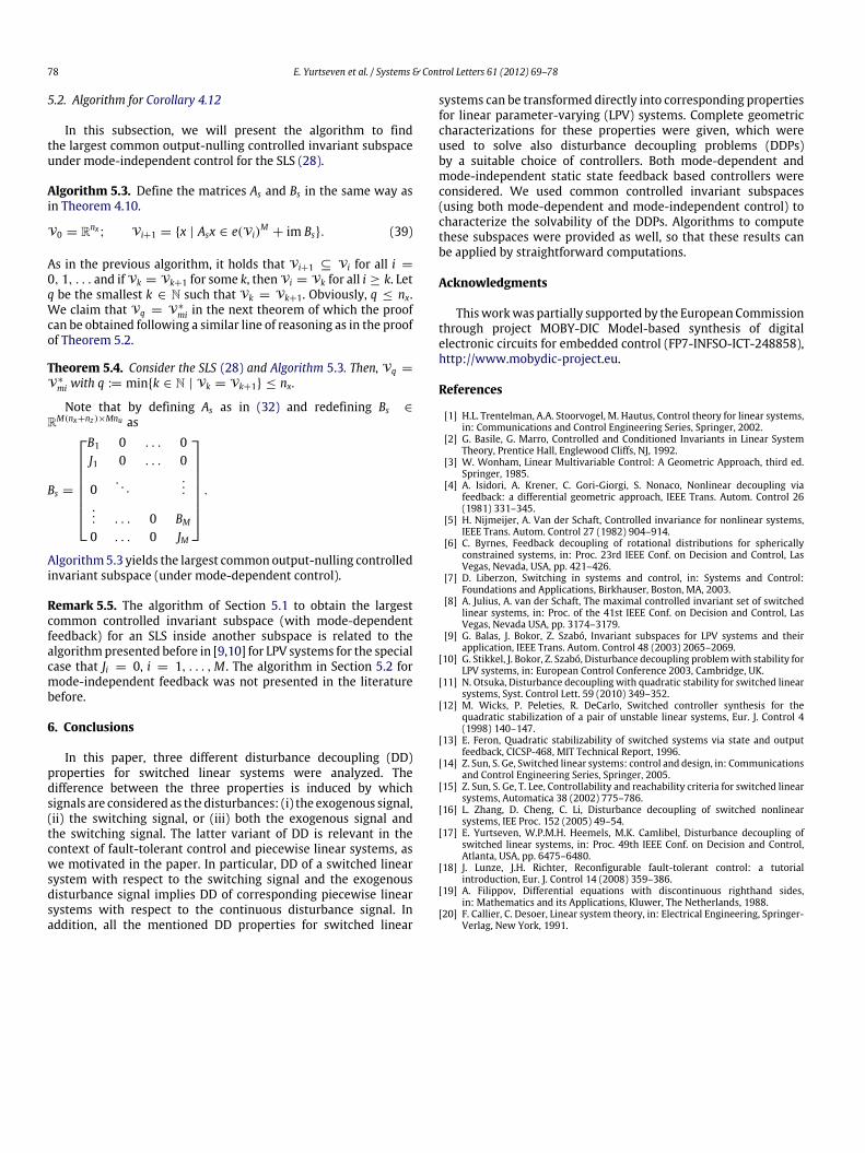
Note that by defining As as in (32) and redefining Bs ∈

RM(nx+nz )×Mnu as

Bs =

B1 0 . . . 0J1 0 . . . 0

0. . .

...

... . . . 0 BM

0 . . . 0 JM

.

Algorithm5.3 yields the largest common output-nulling controlledinvariant subspace (under mode-dependent control).

Remark 5.5. The algorithm of Section 5.1 to obtain the largestcommon controlled invariant subspace (with mode-dependentfeedback) for an SLS inside another subspace is related to thealgorithmpresented before in [9,10] for LPV systems for the specialcase that Ji = 0, i = 1, . . . ,M . The algorithm in Section 5.2 formode-independent feedback was not presented in the literaturebefore.

6. Conclusions

In this paper, three different disturbance decoupling (DD)properties for switched linear systems were analyzed. Thedifference between the three properties is induced by whichsignals are considered as thedisturbances: (i) the exogenous signal,(ii) the switching signal, or (iii) both the exogenous signal andthe switching signal. The latter variant of DD is relevant in thecontext of fault-tolerant control and piecewise linear systems, aswe motivated in the paper. In particular, DD of a switched linearsystem with respect to the switching signal and the exogenousdisturbance signal implies DD of corresponding piecewise linearsystems with respect to the continuous disturbance signal. Inaddition, all the mentioned DD properties for switched linear

systems can be transformed directly into corresponding propertiesfor linear parameter-varying (LPV) systems. Complete geometriccharacterizations for these properties were given, which wereused to solve also disturbance decoupling problems (DDPs)by a suitable choice of controllers. Both mode-dependent andmode-independent static state feedback based controllers wereconsidered. We used common controlled invariant subspaces(using both mode-dependent and mode-independent control) tocharacterize the solvability of the DDPs. Algorithms to computethese subspaces were provided as well, so that these results canbe applied by straightforward computations.

Acknowledgments

Thisworkwas partially supported by the European Commissionthrough project MOBY-DIC Model-based synthesis of digitalelectronic circuits for embedded control (FP7-INFSO-ICT-248858),http://www.mobydic-project.eu.

References

[1] H.L. Trentelman, A.A. Stoorvogel, M. Hautus, Control theory for linear systems,in: Communications and Control Engineering Series, Springer, 2002.

[2] G. Basile, G. Marro, Controlled and Conditioned Invariants in Linear SystemTheory, Prentice Hall, Englewood Cliffs, NJ, 1992.

[3] W. Wonham, Linear Multivariable Control: A Geometric Approach, third ed.Springer, 1985.

[4] A. Isidori, A. Krener, C. Gori-Giorgi, S. Nonaco, Nonlinear decoupling viafeedback: a differential geometric approach, IEEE Trans. Autom. Control 26(1981) 331–345.

[5] H. Nijmeijer, A. Van der Schaft, Controlled invariance for nonlinear systems,IEEE Trans. Autom. Control 27 (1982) 904–914.

[6] C. Byrnes, Feedback decoupling of rotational distributions for sphericallyconstrained systems, in: Proc. 23rd IEEE Conf. on Decision and Control, LasVegas, Nevada, USA, pp. 421–426.

[7] D. Liberzon, Switching in systems and control, in: Systems and Control:Foundations and Applications, Birkhauser, Boston, MA, 2003.

[8] A. Julius, A. van der Schaft, The maximal controlled invariant set of switchedlinear systems, in: Proc. of the 41st IEEE Conf. on Decision and Control, LasVegas, Nevada USA, pp. 3174–3179.

[9] G. Balas, J. Bokor, Z. Szabó, Invariant subspaces for LPV systems and theirapplication, IEEE Trans. Autom. Control 48 (2003) 2065–2069.

[10] G. Stikkel, J. Bokor, Z. Szabó, Disturbance decoupling problemwith stability forLPV systems, in: European Control Conference 2003, Cambridge, UK.

[11] N. Otsuka, Disturbance decoupling with quadratic stability for switched linearsystems, Syst. Control Lett. 59 (2010) 349–352.

[12] M. Wicks, P. Peleties, R. DeCarlo, Switched controller synthesis for thequadratic stabilization of a pair of unstable linear systems, Eur. J. Control 4(1998) 140–147.

[13] E. Feron, Quadratic stabilizability of switched systems via state and outputfeedback, CICSP-468, MIT Technical Report, 1996.

[14] Z. Sun, S. Ge, Switched linear systems: control and design, in: Communicationsand Control Engineering Series, Springer, 2005.

[15] Z. Sun, S. Ge, T. Lee, Controllability and reachability criteria for switched linearsystems, Automatica 38 (2002) 775–786.

[16] L. Zhang, D. Cheng, C. Li, Disturbance decoupling of switched nonlinearsystems, IEE Proc. 152 (2005) 49–54.

[17] E. Yurtseven, W.P.M.H. Heemels, M.K. Camlibel, Disturbance decoupling ofswitched linear systems, in: Proc. 49th IEEE Conf. on Decision and Control,Atlanta, USA, pp. 6475–6480.

[18] J. Lunze, J.H. Richter, Reconfigurable fault-tolerant control: a tutorialintroduction, Eur. J. Control 14 (2008) 359–386.

[19] A. Filippov, Differential equations with discontinuous righthand sides,in: Mathematics and its Applications, Kluwer, The Netherlands, 1988.

[20] F. Callier, C. Desoer, Linear system theory, in: Electrical Engineering, Springer-Verlag, New York, 1991.