Distributed Monitoring of Voltage Collapse Sensitivity Indices

1

Distributed Monitoring of Voltage Collapse

Sensitivity IndicesJohn W. Simpson-Porco, Member, IEEE, and Francesco Bullo, Fellow, IEEE

Abstract—The assessment of voltage stability margins is apromising direction for wide-area monitoring systems. Accuratemonitoring architectures for long-term voltage instability aretypically centralized and lack scalability, while completely decen-tralized approaches relying on local measurements tend towardsinaccuracy. Here we present distributed linear algorithms forthe online computation of voltage collapse sensitivity indices. Thecomputations are collectively performed by processors embeddedat each bus in the smart grid, using synchronized phasormeasurements and communication of voltage phasors betweenneighboring buses. Our algorithms provably converge to theproper index values, as would be calculated using centralizedinformation, but but do not require any central decision makerfor coordination. Modifications of the algorithms to account forgenerator reactive power limits are discussed. We illustrate theeffectiveness of our designs with a case study of the New England39 bus system.

Index Terms—Distributed monitoring, smart grid, voltagecollapse, voltage stability, wide-area monitoring and control

I. INTRODUCTION

Power grids are transitioning from a paradigm of centralized

monitoring and control to one based on decentralized deci-

sions and consumer interaction. When coupled with waining

infrastructure investment, rapidly growing urban load centers,

and the wide-spread adoption of intermittent distributed gen-

eration, this structural shift will lead to a broader and more

uncertain range of operating conditions for the grid and an

erosion of system stability margins if not properly coordinated.

Simultaneously however, the rise of cheap and ubiquitous

sensing, communication, and computational capabilities sug-

gest a future where the physical grid is strongly coupled to

many accompanying layers of data and control. Unlike classic

grids where sparsely available information is telemetered to a

control center and processed, copious amounts of information

are distributed throughout the smart grid along with the com-

putational capabilities to process the measured data and make

coordinated decisions in real-time for wide-area monitoring,

protection, and control (WAMPAC) [1], [2]. The distributed

nature of these smart grid resources suggests we explore and

evaluate the effectiveness of different information architectures

for WAMPAC, ranging the spectrum from centralized to

decentralized.

In this article we consider the problem of online monitoring

for long-term voltage instability (LTVI) within a smart grid,

J. W. Simpson-Porco is with the Department of Electrical and ComputerEngineering, University of Waterloo, Waterloo ON, N2L 3G1 Canada. Corre-spondance: [email protected]. F. Bullo is with the Center forControl, Dynamical Systems and Computation, University of California, SantaBarbara, CA 93106 USA. This work was supported by NSF CNS-1135819and by the Natural Science and Engineering Research Council of Canada.

which has recently been identified as an area of urgent interest

for industry [3]. While in general voltage stability is a com-

plex, multi time-scale phenomena, long-term voltage instabil-

ity is a quasi-static bifurcation instability [4], [5] associated

with an inability of the combined generation/transmission

system to transmit sufficient power to loads [6]. After an

increase in load, or a disturbance such as generation failure

or load shedding, the grid’s long-term operating point can

vanish leading to the tripping of protection equipment and

potentially to a large-scale voltage collapse blackout [6].

Robustness margins against LTVI are quantified via voltage

collapse proximity indices (VCPIs), which produce measures

of distance to instability [7]. Accurate indicator estimates

are key for distinguishing vulnerable system conditions from

stable conditions exhibiting low voltages [8], and we now

review various architectures for the calculation of such indices.

A. Monitoring of Long-Term Voltage Instability

Many monitoring solutions for LTVI have been proposed,

and can be broadly classified by architecture (centralized, de-

centralized, distributed), measurement rate/complexity (time-

skewed SCADA vs. time-stamped phasor measurement unit

data), and theoretical rigor (heuristic vs. exact) [8]. The

most important distinction for our purposes is monitoring

architecture, which we now expand on.

Centralized Monitoring: In a centralized monitoring ap-

proach, relevant data is telemetered to a central computer in a

control center and potentially combined with state estimation

to calculate relevant indices; see [8]–[11] and the many

references therein. From the perspective of this paper, the

main drawback of a centralized approach is that it results

in a single point of failure for the monitoring system, and

potentially requires data to be sent over large distances. Data

privacy issues may also come into consideration. Moreover, in

emerging applications such as microgrids, centralized super-

vision may be untenable or prohibitive. In this case, a more

modular, scalable monitoring approach is desirable.

Decentralized Monitoring:∗ In contrast to centralized

monitoring, decentralized techniques rely only on locally

measured information to estimate voltage stability margins.

Monitoring techniques based on PMU data and/or Thevenin

equivalent circuits were proposed in [12]–[16], among others.

Decentralized VCPIs offer low implementation complexity and

∗We use the term decentralized here for what is sometimes called “com-pletely decentralized” or “completely distributed” — the VCPI calculated atbus i will depend only on information measured locally at bus i, such as thephasor voltage Vi∠θi and the complex power injection Pi + jQi.

Digital Object Identifier: 10.1109/TSG.2016.2533319

1949-3061 c© 2016 IEEE. Personal use is permitted, but republication/redistribution requires IEEE permission.See http://www.ieee.org/publications standards/publications/rights/index.html for more information.

2

easy scalability, with the additional advantage that (typically)

no communication or state estimation is required. The price

paid for these advantages is accuracy: decentralized VCPIs

are invariably heuristics, often inspired by single-line power

flow results, and are always too optimistic since they do not

explicitly account for the electrical coupling between buses

[17]. A notable exception for decentralized approaches is [17],

where sensitivities of voltages with respect to on-load tap

changer ratios are used to monitor the system for instability.

A monitoring approach for LTVI was presented in [18],

where the grid is partitioned into overlapping monitoring areas

(akin to control areas in automatic generation control). The

indices used however are somewhat unconventional, and the

approach relies on selecting monitoring areas which are only

weakly coupled. Neglecting this small inter-area coupling then

results in a centralized assessment problem within each area.

While being termed “distributed”, in our terminology the

approach in [18] is a hybrid of centralized and decentralized

ideas. In Remark 3 we comment on the extension of our

distributed approach to a similar multi-area architecture.

Distributed Monitoring: In the intermediate between cen-

tralized and decentralized we arrive at distributed monitor-

ing strategies, which rely on local measurements along with

communicated data from directly adjacent buses or areas

of the grid. Distributed strategies promise to combine the

performance of centralized monitoring with the scalability

of decentralized monitoring, requiring only sparse, localized

communication without global information or coordination.

Reflecting this, the recent literature has witnessed a steady

growth in the applications of distributed algorithms to power

system monitoring and control, now including resource alloca-

tion [19], load shedding [20], economic dispatch [21], optimal

power flow [22], voltage control [23], transfer capability

assessment [24], and inverter coordination in microgrids [25].

To the authors knowledge however, distributed algorithms

have not yet been designed for the monitoring of VCPIs. In

particular, we focus on a subclass of VCPIs termed sensitivity

indices, which quantify the sensitivity of grid states to changes

in grid parameters. These sensitivities increase as voltage

collapse is approached, and monitoring these sensitivities

therefore provides information on the proximity to collapse.

B. Contributions

In this work we present the first distributed algorithms for

the online computation of voltage collapse sensitivity indices.

We demonstrate that the exact calculation of several standard

centralized indices can be distributed among agents embed-

ded within the smart grid, achieving centralized performance

through only local measurements and short-range nearest-

neighbor communication. The exact nature of these agents

is left unconstrained; the software could be embedded in

next generation power inverters, power electronic devices for

voltage control, or implemented at generators or smart meters.

Our algorithms do not rely on a state estimator processing

sparse measurements to estimate state variables, but rather

combine direct local measurements with measurements made

and communicated by neighboring buses. Data is transmitted

only over short distances, minimizing communication prob-

lems such as packet delays and measurement problems such

as time-stamp drift. No centralized decision maker is required.

Our approach does not rely on any pre-defined interfaces, on

any representative sets of offline data used for learning, or

on any Thevenin equivalent representations. After algorithm

convergence, each bus recovers its exact sensitivity index along

with the indices of neighboring buses. We demonstrate the

efficacy of our algorithms via simulation in Section IV on the

IEEE 39 bus system.

We assume that each bus in the system is equipped with

a phasor measurement unit. While current power systems

are not equipped with this level of observability, the smart

grid eventually may, and demonstrations of the operational

benefits of observability (such as those presented herein) will

serve as incentive to invest in such measurement capabilities

in the future. It seems plausible that our assumption of full

observability can be relaxed, and that the approach can be

extended to more detailed models of long-term voltage insta-

bility, but we defer further discussion of this to our concluding

remarks in Section V. At the transmission level, centralized

state estimation-based VCPIs will continue to play a major

role, but it is nonetheless important to assess the advantages

and limitations of alternative architectures. Our main message

is that complicated sensitivity indices can in fact be com-

puted using only localized information, without the need for

centralized coordination or computation. An area where our

algorithms may prove particularly useful is microgrids, where

centralized monitoring, control and optimization architectures

are often absent and must be implemented collectively by

coordinating devices within the microgrid in a scalable way.

C. Preliminaries and Notation

We let R (resp. R>0) denote the set of real (resp.

strictly positive real) numbers. Given x ∈ Rn, ‖x‖∞ =maxi∈{1,...,n} |xi|, and [x] ∈ Rn×n is the associated diagonal

matrix with x on the diagonal. Throughout, 1n and 0n are

the n-dimensional vectors of unit and zero entries, and 0 is

a matrix of all zeros of appropriate dimensions. The n × nidentity matrix is In.

II. SYSTEM MODELS AND SENSITIVITY-BASED VOLTAGE

COLLAPSE PROXIMITY INDICES

We begin by defining the grid models to be used in the

paper before reviewing the relevant voltage collapse indices.

A. Power System Model

We model a balanced, quasi-synchronous power grid as a

connected, undirected and weighted graph (V, E), where V is

the set of nodes (buses) and E ⊆ V × V is the set of edges

(branches). We partition the set of buses V as V = L∪G, with

n ≥ 1 load (PQ) buses L = {1, . . . , n} and m ≥ 1 generator

(PV) buses G = {n+1, . . . , n+m}.† Each branch {i, j} ∈ E

†For our purposes, load buses L may represent either standard loads orinverters performing maximum power point tracking. Similarly, generatorbuses G may represent synchronous generators, frequency-dependent loads,or grid-forming inverters implementing droop control [21], [26].

3

is weighted by a transfer admittance yij = gij + jbij , where

gij ≥ 0 and bij ≤ 0. We encode the weights and topology in

the bus admittance matrix Y , with elements Yij = −yij and

Yii =∑n+m

j 6=i yij+yshunt,i, where yshunt,i is the shunt element

at bus i. The conductance matrix G and susceptance matrix

B are defined by G = Re(Y ) and B = Im(Y ). To each bus

i ∈ V we associate a phasor voltage Vi∠θi and a complex

power injection Pi+jQi, which are related by the power flow

equations

Pi =∑

j∈VViVj(Gij cos(θi − θj) +Bij sin(θi − θj)) , (1a)

Qi =∑

j∈VViVj(Gij sin(θi − θj)−Bij cos(θi − θj)) . (1b)

The unknowns in (1a)–(1b) are the phase angles θ =(θ1, . . . , θn+m) and the load voltages VL = (V1, . . . , Vn).With shunt admittances absorbed into the admittance matrix,

we assume that the remainder of the load at each PQ bus can

be described by a constant power load model. Extending our

approach to more general voltage-dependent static load models

Pi(Vi) and Qi(Vi) is straightforward, and requires only a few

additional terms in the formulae and algorithms which follow;

we omit these extensions for notational simplicity. Further

comments on grid modeling are deferred to Section V.

B. Cyber Layer Model

We assume that devices (agents) are embedded at each

bus i ∈ V and are capable of measuring local information,

communicating with devices at nearby buses, and performing

basic computations on the measured data.

Regarding measurement, we assume that each bus i ∈ Vis equipped with a PMU, yielding accurate and synchronized

measurements of voltage phasors Vi∠θi. In addition we as-

sume that the processor at each bus has knowledge of (or

access to measurements of) power system infrastructure inci-

dent to the bus, such as local power consumption/generation

Pi + jQi, the admittances of incident electrical lines yij ,

and any local shunt elements yshunt,i. Admittances may be

know a priori, or estimated in an initialization phase using

ranging technologies over power line communication (PLC)

channels. Similarly, shunt susceptances designed to support

voltage magnitudes are often either fixed or switched by

local controllers which could be integrated into the processing

equipment under consideration. In contrast to SCADA systems

which sample data every few seconds, PMUs under the IEEE

Standard C37.118 [27], [28] are synchronized and able to take

10’s of samples per second. On the time scales of interest for

LTVI, this fast sampling is well approximated as continuous-

time measurement. Throughout we assume high-quality mea-

surements, and do not distinguish between measured and true

values of variables. If PMU measurement quality is determined

to be an issue, a distributed state-estimation and filtering layer

[29], [30] can be implemented between the raw measurements

and our algorithms to improve signal-to-noise ratios and reject

bad data.

Regarding communication, we assume that each agent can

communicate bidirectionally with the agents at adjacent buses

to which it is electrically connected. Said differently, the

topology of the communication layer mimics the physical

grid topology. This communication could be achieved through

power line communication (PLC), limited-range wireless, or

Ethernet. We emphasize that here our focus is not on detailed

communication protocols, but on highlighting the sufficiency

of local information exchange for the exact calculation of

standard sensitivity indices. To streamline our mathematical

developments throughout, we will therefore assume generous

communication capabilities which in effect permit continuous-

time communication. Due to the large separation of time-scales

between PMU sampling rates and LTVI, and the fact that

our algorithms require only short-distance communications,

throughout we assume that delays are negligible. Nonetheless,

in Remark 2 we comment on theoretical extensions to less

restrictive communication assumptions.

C. Sensitivity-Based Voltage Collapse Proximity Indics

As LTVI and voltage collapse are associated with saddle-

node bifurcation of the network’s equilibrium equations, sin-

gularity of the power flow Jacobian or related matrices has

long been used as an indicator of voltage collapse [31].

Related approaches include modal analysis, singular value

and condition number indices, sensitivity indices, continuation

methods, optimization, and energy function-based VCPIs. Sur-

veys, classifications, and comparative studies of various VCPIs

are available in [6]–[8], [32]–[39].

Here we focus on one of the oldest classes of VCPIs, the

sensitivity indices, which are based on the sensitivity of the

system operating point to variations in parameters. The idea

is that small variations in system parameters — for example,

load demands — will produce large variations in bus voltages

near bifurcation [32], [40], [41]. While many sensitivity-

based VCPIs have been superseded in practical power system

operations by more accurate, more computationally intensive

techniques, they nonetheless provide intuitive actionable in-

formation, and are relatively straightforward to define and

interpret. We recall three basic indices [42, Sec. 8.2.3] and

then comment on the information needed to compute them.

All derivatives are evaluated at the current operating point.

a) The “dV/dQ” Index: This index measures the sensi-

tivity of load bus voltage magnitudes with respect to changes

in reactive power demands. For a multi-bus network, for each

load bus i ∈ L we may formulate the appropriate indicator as

Ii ,∑

j∈LQj

Vi

δVi

δQj

, i ∈ L . (2)

The summands are the point elasticities of the voltage at load

bus i with respect to the reactive injection at load bus j. The

sum then evaluates the total elasticity of the voltage at bus

i ∈ L. The index ranges from 0 at open-circuit conditions to

+∞ when the system reaches the point of collapse.

b) The “dVL/dVG” Index: Also called the “dV/dE”

index, this index measures the sensitivity of load bus voltages

to changes in generator grid-side voltage set points. The

appropriate multi-bus index Ji is

Ji ,∑

k∈GδVi

δVk

, i ∈ L . (3)

4

Near open-circuit conditions Ji should be near unity, indicating

that changes in load voltages track changes in generator

voltages with unity gain (a “controllability” property [32]).

The index tends to +∞ at the point of collapse.

c) The dQG/dQL Index: This index measures the in-

cremental reactive power generation required to supply an

incremental amount of additional load, and therefore quantifies

the (inverse) efficiency of reactive power transport through the

network. The appropriate multi-bus definition is

Ki ,∑

k∈GδQk

δQi

, i ∈ L . (4)

With our sign conventions, the Ki ranges from −1 at open-

circuit to −∞ at bifurcation, indicating that the network

transports reactive power inefficiently near voltage collapse.

The important observations regarding the indices (2)–(4)

are (i) the matrices of derivatives defining them are generally

dense matrices, and (ii) the matrix elements take into account

the global state of the network. For example, for a processor

at bus i ∈ L to directly compute Ji, it would need to not

only be directly aware of all generators connected to the

network, but also know numerically how variation of the set

points Vk of each generator influence the local voltage Vi. This

sensitivity is in turn influenced by the presence (or absence)

of loading/compensation at all other buses. Ostensibly then,

(2)–(4) incorporate non-local information, and it would appear

then that only an operator with centralized or near-centralized

state information can evaluate them.

III. DISTRIBUTED COMPUTATION OF SENSITIVITY-BASED

VCPIS

We now detail our approach for distributing the computation

of the VCPIs presented in Section II-C. We present our ap-

proach pedagogically for the dV/dQ index (2) before formally

defining our distributed protocols for all indices (2)–(4) and

addressing protocol convergence. To begin, note that in vector

notation the dV/dQ index (2) becomes

I = [VL]−1 δVL

δQL

QL ,

where I = (I1, . . . , In), QL = (Q1, . . . , Qn), [VL] is the

diagonal matrix of load bus voltages, and δVL/δQL is the

matrix with elements δVi/δQj for load bus indices i, j ∈ L.

Away from the point of collapse the matrix δVL/δQL is

invertible, and we may equivalently write

δQL

δVL

[VL]I = QL , (5)

which is a (dense) system of equations for I. Returning to

the power flow (1a)–(1b), around an operating point (θ, VL) ∈Rn+m × Rn

>0 incremental changes (δθ, δVL, δVG) in phase

angles, load voltages, and generator voltage set points are

related to incremental changes (δP, δQL, δQG) in active and

reactive power injections (load and generator) by

δPδQL

δQG

=

∂P∂θ

∂P∂VL

∂P∂VG

∂QL

∂θ∂QL

∂VL

∂QL

∂VG

∂QG

∂θ∂QG

∂VL

∂QG

∂VG

δθδVL

δVG

. (6)

If variations in active power injections δP and generator

voltages δVG are held at zero, the first two block-rows of

equations in (6) may be solved to yield

δQL

δVL

=∂QL

∂VL

−∂QL

∂θ

(

∂P

∂θ

)†∂P

∂VL

. (7)

where † denotes the Moore-Penrose pseudoinverse (see Re-

mark 1). The system of equations (5) for I then becomes

∂QL

∂VL

[VL]I−∂QL

∂θ

(

∂P

∂θ

)†∂P

∂VL

[VL]I = QL .

Introducing an auxiliary variable Iaux ∈ Rn+m, this dense

system of equations is equivalent to the expanded system(

∂QL

∂VL[VL]

∂QL

∂θ

∂P∂VL

[VL]∂P∂θ

)

(

I

Iaux

)

=

(

QL

0n+m

)

. (8)

The coefficient matrix in (8) is sparse, its sparsity pattern

closely related the physical grid topology. Indeed, the sparsity

of such matrices has long been used as an aid for fast

computation of stability margins [43]. While sparsity of the

unreduced Jacobian (6) could also be exploited for computing

the desired indices, (6) will typically contain unnecessary in-

formation, which for our algorithms would lead to unnecessary

communication and computation. For example, the third block-

row in (6) contains unnecessary information for the dV/dQindex. We therefore find the reduced Jacobian-like matrix

in (8) more useful to work with. To propose the simplest,

most intuitive distributed algorithm for calculating the stability

index I, we make the following assumptions.

Assumption 1 (System Matrix Stability): All eigenvalues of

the matrices

∂P

∂θ,

(

∂P∂θ

∂P∂VL

∂QL

∂θ∂QL

∂VL

)

,

(

∂P∂θ

∂P∂VL

[VL]

∂QL

∂θ∂QL

∂VL[VL]

)

.

have positive real parts, with the exception of a simple zero

eigenvalue for each with respective right eigenvectors 1n+m,

(1n+m, 0n) and (1n+m, 0n).Remark 1 (Comments on Assumption 1): The simple zero

eigenvalues of the matrices in Assumption 1 correspond to a

uniform shift δθ 7→ δθ+α1n+m of all phase angle deviations

δθ. Since phase is defined only up to a reference, this trivial

degree of freedom may be removed by restricting Iaux to lie

in the subspace orthogonal to 1n+m, in which case all three

matrices are effectively invertible. In practice Assumption 1

holds away from the point of collapse [34], and the non-zero

eigenvalues of these matrices are often found to be real or

have small imaginary parts [44, Appendix B.3]. Moreover,

Assumption 1 is quite natural since (i) the matrices under

consideration describe stable small-signal behavior for certain

classes of power system dynamics, and (ii) these dynamics are

known to not exhibit Hopf bifurcations, and hence the respec-

tive matrices can only become singular when an eigenvalue

reaches the origin during saddle-node bifurcation [5]. In this

sense then, Assumption 1 is “necessary and sufficient” for the

linear system (8) to be well-posed. �

Our key observation is that the matrix elements in (8) are

determined by localized information: the ijth element of any

5

sub-matrix depends only on the voltage phasors at buses i and

j and on the admittance of the adjoining branch. It follows that

by using phasor measurements and communication among ad-

jacent buses, the solution of (8) for (I, Iaux) can be distributed

among processors embedded at each bus. With this goal in

mind, to each load bus i ∈ L we associate a pair of scalar states

(xi, yi) ∈ R2, while to each generator bus i ∈ G we associate

a scalar state yi ∈ R. We assume that these states can be

communicated bidirectionally between directly adjacent buses.

Our first formal result gives a simple distributed algorithm in

continuous-time such that limt→∞ xi(t) → Ii for each i ∈ L.

For notational convenience we define the data coefficients

dij , ViVj (Gij sin(θi − θj)−Bij cos(θi − θj)) , (9a)

Dij , ViVj (Gij cos(θi − θj) +Bij sin(θi − θj)) , (9b)

for each i, j ∈ V , which depend only on known constants,

locally measured PMU data, and PMU data communicated

between adjacent buses in the grid.

Theorem 3.1 (Distributed dV/dQ Index): Consider the

dV/dQ indices Ii defined in (2) and let dij and Dij be as in

(9). Let each load bus i ∈ L execute

τ xi = Qi(1− xi)− Piyi −∑

j∈Ldijxj +

∑

j∈VDijyj , (10a)

τ yi = Qiyi − Pixi −∑

j∈LDijxj −

∑

j∈Vdijyj , (10b)

for some chosen τ > 0, while each generator bus i ∈ Gexecutes

τ yi = Qiyi −∑

j∈LDijxj −

∑

j∈Vdijyj . (11)

Then for any initial condition (x(0), y(0)) ∈ Rn × Rn+m it

holds for each i ∈ L that limt→∞ xi(t) = Ii.

Proof: Let x = (x1, . . . , xn) and y = (y1, . . . , yn+m) be the

state vectors associated with (10)–(11). Comparing the right-

hand sides of (10)–(11) with the power flow Jacobian matrix

elements in Lemma A.1, one finds that in vector notation (10)–

(11) reads as

τ

(

xy

)

= −

(

∂QL

∂VL[VL]

∂QL

∂θ

∂P∂VL

[VL]∂P∂θ

)

(

xy

)

+

(

QL

0n+m

)

. (12)

Conversely, (10)–(11) are obtained by writing out (12) in

components, using Lemma A.1 and the definitions of dij and

Dij in (9). Comparing the dynamics (12) to the algebraic

equation (8), it follows that the steady-states of (10)–(11)

are one-to-one correspondence with the solutions (I, Iaux) of

(8). The system matrix in (12) is a permutation of the third

matrix in Assumption 1, and is therefore Hurwitz except for

a simple eigenvalue at zero with normalized right eigenvector

u1 = (0n,1√

n+m1n+m). The component of the state which

evolves parallel to u1 only influences the (average value of

the) auxiliary variable y(t), and does not influence the index

estimates x(t). Since by assumption all other eigenvalues have

negative real parts, it follows that limt→+∞ x(t) = I, which

completes the proof. �

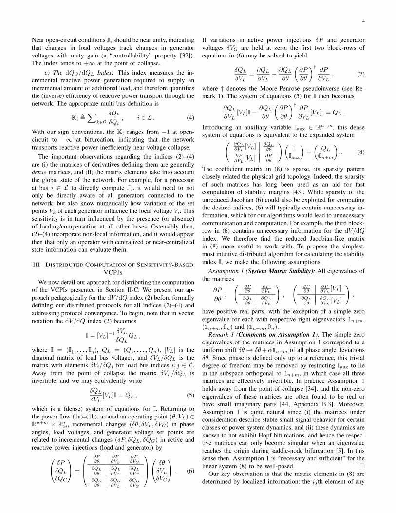
Fig. 1. Depiction of monitoring architecture for a radial three bus power sys-tem implementing the algorithm (10)–(11). Synchrophasor data is measuredand fed to local processors, while communication between adjacent processorstransfers both synchrophasor measurements Vi∠θi and filter states xi, yi.

The monitoring architecture is depicted in Figure 1 for a

simple power system. While the sums in (10)–(11) run over

all loads or all buses, the coefficients dij and Dij are zero

when {i, j} is not a physical branch of the network, and

hence the only information needed at processor i ∈ V is that

from electrically adjacent buses. Said differently, the proposed

monitoring architecture requires only peer-to-peer communi-

cation, without centralized coordination. Uniformity of the

time constant τ across all buses is formally required to infer

stability, but as our case study in Section IV will demonstrate,

mildly nonuniform time constants τi pose no difficulties when

implemented, and can thus be chosen independently.

We make five observations regarding the above algorithm.

First, note that the storage and computational requirements for

implementation are extremely low. Each agent stores only the

local states (xi(t), yi(t)) or yi(t), and integrates an ordinary

differential equation; storing the time-history of states is not

required, nor is it required that each agent maintains an

estimate of the entire algorithm state. Second, the method

relies only on bus measurements, and no measurements of

branch currents are required. Third, communication is required

only between neighboring buses in the network, minimizing

the effects of any communication delays. Fourth, the time

variable t in the algorithm should be interpreted as a com-

putational time-scale; the time constant τ can be adjusted

to achieve any desired convergence speed, limited ultimately

by communication time scales, measurement sampling time,

and system dynamics, but not by the algorithm itself. Fifth

and finally, our method does not rely on a linearized power

flow model; the linearity of (10)–(11) comes from examining

sensitivities of the nonlinear power flow (1a)–(1b), with real-

time measurements replacing a nonlinear power flow solver.

Remark 2 (Relaxed Algorithms & Communications): As

one can see from (12), the distributed algorithm (10)–(11)

is of the form τ v = −Av + b, and hence can be explic-

itly discretized for distributed synchronous implementation as

v(k + 1) = (I2n+m − hA/τ)v(k) + hb/τ for a time-step

6

h > 0. Under Assumption 1, this discrete-time system is

stable if and only if h < 2τ maxiRe(λi)|λi|2 . Another option

for distributed implementation is Jacobi iteration, where Ais decomposed into its diagonal part T = diag(aii) and off

diagonal part R = A − T , with the iteration taking the form

v(k + 1) = T−1(b − Rv(k)). This iteration converges if and

only if ρ(T−1R) < 1; the authors have observed numerically

that this assumption often holds for the relevant matrices in

Assumption 1, but in general this assumption and Assumption

1 are not equivalent. The easily verified diagonal dominance

conditions for stability of the Jacobi iteration do not hold.

Packets from neighbors may arrive asynchronously or with

delays, and communication may be event-triggered, based on

sufficient changes in local measurements. While our focus is

not on detailed communication protocols, we note a particular

approach which is more complex but less restrictive. In [45]

a discrete-time algorithm was developed for the distributed

solution of linear equations such as (8). In the proposed

approach, each bus is assumed to know its respective row of

the coefficient matrix, and updates a local estimate of the entire

system state (x, y) by exchanging estimates with neighbors.

Thus, the requirements on information and communication are

similar to the ones required by Theorem 3.1, with slightly more

local storage requirements. The approach extends to handle

both asynchronism and delays [46], [47]. When Assumption

1 fails during extreme system conditions, the algorithm (10)–

(11) will diverge, and one of these alternatives would be

required to calculate the relevant indices (which may even

change sign under such conditions). �

Remark 3 (Extension to Multi-Area Monitoring): While

we have presented the algorithm (10)–(11) with a direct peer-

to-peer implementation, it is easily extended to the case of

multi-area monitoring. To see this, partition the the buses V of

the network into p ≤ n+m non-overlapping monitoring areas

V = A1 ∪ · · · ∪Ap. Depending on the specific problem setup,

these areas could correspond to ISO regions, substations,

phasor data concentrators (PDCs), or microgrids. Inside area

Ak, assume that a central processor Pk has (i) access to PMU

measurements from each bus in area Ak (ii) knowledge of the

grid topology and parameters in area Ak (iii) knowledge of the

power lines which connect Ak to neighboring areas, and (iv)

the ability to perform basic computations and communicate

data with the processors in neighboring areas. In this case, the

algorithm (12) would simply be block-partitioned according to

the different areas, with central processors implementing the

required blocks. The case of one area p = 1 would correspond

to complete centralized monitoring, where a central processor

aggregates all information and performs all computations,

while p = n + m is the case described in main paper,

where each bus (e.g., substation) constitutes an area, only

local measurements are required, and information exchange is

peer-to-peer. Depending on regional data disclosure policies

and privacy concerns, one architecture may be preferable over

another; these issues are outside the scope of this work. �

Similar filters to (10)–(11) can be designed to calculate the

dVL/dVG index (3) and the dQG/dQL index (4); the proofs

may be found in Appendix A.

Theorem 3.2 (Distributed dVL/dVG Index): Consider the

dVL/dVG indices Ji defined in (3) and let dij and Dij be as

in (9). Let each load bus i ∈ L execute

τ xi = −Qi

Vi

xi − Piyi −∑

j∈L

dijVj

xj +∑

j∈VDijyj −

∑

j∈G

dijVj

,

τ yi = Qiyi −Pi

Vi

xi −∑

j∈L

Dij

Vj

xj −∑

j∈Vdijyj −

∑

j∈G

Dij

Vj

,

for some chosen τ > 0, while each generator bus i ∈ Gexecutes

τ yi = −Pi

Vi

+Qiyi −∑

j∈L

Dij

Vj

xj −∑

j∈Vdijyj −

∑

j∈G

Dij

Vj

.

Then for any initial condition (x(0), y(0)) ∈ Rn × Rn+m it

holds for each i ∈ L that limt→∞ xi(t) = Ji.

Theorem 3.3 (Distributed dQG/dQL Index): Consider the

dQG/dQL indices Ki defined in (4) and let dij and Dij be

as in (9). Let each load bus i ∈ L execute

τ xi = −Qi

Vi

xi −Pi

Vi

(yi − zi)−∑

j∈L

djiVi

xj

−∑

j∈V

Dji

Vi

(yj − zj) +∑

j∈G

djiVi

,

τ yi = Qiyi − Pixi +∑

j∈LDjixj −

∑

j∈Vdjiyj ,

τ zi = Qizi −∑

j∈Vdjizj +

∑

j∈GDji ,

for some chosen τ > 0, while each generator bus i ∈ Gexecutes

τ yi = Qiyi +∑

j∈LDjixj −

∑

j∈Vdjiyj ,

τ zi = −Pi +Qizi −∑

j∈Vdjizj +

∑

j∈GDji ,

Then for any initial condition (x(0), y(0), z(0)) ∈ Rn ×Rn+m × Rn+m it holds for each i ∈ L that limt→∞ xi(t) =Ki.

A. Incorporating Generator VAR Limits

The distributed algorithms presented in Theorems 3.1–

3.3 ignore an important factor in LTVI studies, namely the

reactive power limitations of generators [48]–[50]. When a

synchronous generator exceeds these reactive power limits

(derived from field and armature current limits) over medium

time-scales, the AVR system becomes unable to regulate the

network-side generator voltage and over-excitation limiters fix

the reactive power output at its limit. On the long-time scales

of interest for us, we can therefore approximate this behavior

by replacing the PV bus model with a PQ bus model when

the generator is at or above its reactive power limit [44].

The approach for incorporating these limits into the dis-

tributed algorithm (10)–(11) of Theorem 3.1 is as follows

(similar approaches hold for the remaining two algorithms).

If the reactive power supplied by generator i ∈ G satisfies

Qi < Qmaxi , then the associated processor executes (11),

7

just as before. When Qi ≥ Qmaxi , the processor initializes

an additional internal state xi(t) and instead executes (10a)–

(10b). If necessary, this can be accompanied with a binary

alert message to its neighbors signaling that a switch has taken

place. To avoid chattering due to oscillating reactive power

injections during transients, a temporal hysteresis can be used

which ensures that Qi remains above or below Qmaxi for a

sufficient amount of time before a switch in algorithm is made.

B. Monitoring Thresholds and Worst-Case Indices

The algorithms in Theorems 3.1–3.3 give the processor at

load bus i ∈ L a converging estimate of its stability index Ii, Jior Ki, as well converging estimates of the same indices for

any adjacent buses which are also load buses. Based on this

information, we highlight two additional steps for monitoring

that may be desirable. We discuss the dV/dQ algorithm (10)–

(11); similar statements apply to the other algorithms.

Monitoring Thresholds: Suppose that to each load bus

i ∈ L we associate a threshold γi > 0 for the index Ii. These

thresholds may be determined by experience, offline trials, or

determined online by yet another distributed algorithm. If dur-

ing monitoring xi(t) increases above γi and remains there, an

alert is triggered and communicated to neighboring processors.

This in turn could trigger localized control responses, or the

alert could be propagated system-wide.

Global Knowledge of Worst-Case Index: Voltage stability

of the network is ultimately limited by the weakest or most

sensitive bus, quantified in our setup by the largest nodal value

‖I‖∞ = maxi∈L Ii of the stability index. It may therefore be

desirable for all buses to maintain an estimate wi(t) of the

worst-case index ‖I‖∞ and continuously update it. A simple

distributed protocol for achieving this is called max-consensus

[51], [52] where each processor executes (in discrete-time)

wi(k + 1) = max

{

wi(k), maxj,{i,j}∈E

wj(k)

}

, (15)

with the initialization wi(t0) = xi(t0) for i ∈ L, where t0is the time at which execution begins. As generator buses

i ∈ G do not carry a local state xi(t), each wi(t0) is

initialized to a common value w∗ for each i ∈ G, equaling

the open-circuit value of the voltage stsability index under

consideration. For example, for the dV/dQ index w∗ = 0,

while for the dVL/dVG index w∗ = 1. Each processor

observes its own index and the indices of its neighbors and

updates its estimate with the largest value it sees. By re-

initializing and re-executing this periodically, all processors

in the network can be made aware of the largest sensitivity.

IV. CASE STUDY: IEEE 39 BUS SYSTEM

We demonstrate our approach by implementing our algo-

rithm for the dVL/dVG index of Theorem 3.2 on a dynamic

model of the reduced New England power grid, containing 9

generators and 30 load buses. A six-state two-axis model is

used for the generators consisting of two-state mechanical dy-

namics, two-state electrical dynamics, a single-state excitation

system and a single-state governor with droop [53]; generator

and network parameters are drawn from [53]–[55].

In place of a uniform filter time constant τ , we let each

processor implement its dVL/dVG filter with a time constant

τi, which we draw from a uniform distribution between 10s

and 20s. Synchrophasor measurements are assumed to be

corrupted with uncorrelated zero mean Gaussian noise, with

standard deviation 0.001 p.u. on voltage magnitudes (arising

from quantization and harmonic distortion), and 0.01◦ on

phase angles (due to sampling time discrepancies and inexact

synchronization). At a 2σ level, these values are in compliance

with the maximum total phasor error of 1% specified by IEEE

Standard C37.118-2011 [28]. Beginning from the base load

case [55], power demands are ramped along the base case by

15% between t = 20s and t = 40s, with the newly ramped

load being shed abruptly at t = 200s.

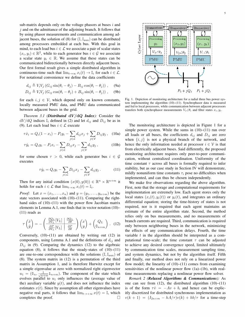
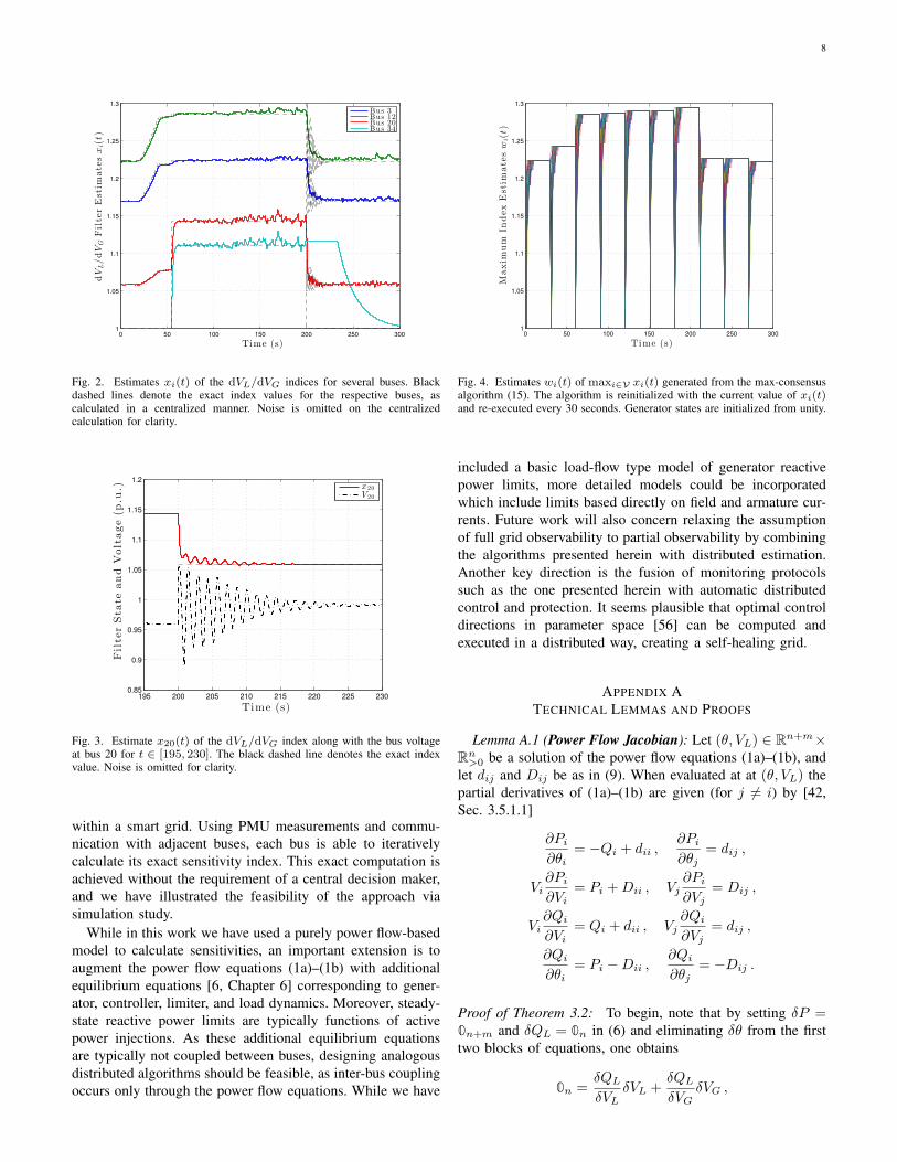
The filter states xi(t) are plotted in Figure 2 for load

buses 3, 12, and 20, and the generator bus 34 whose state

is initialized as x34(0) = 1. The exact steady-state values

of the respective stability indices are plotted in dashed black

for each bus, as computed by a central processor solving the

linear equation (16) at each moment in time. First, we observe

that the algorithm is able to accurately track the ramp in load

between 20s and 40s. The estimates for buses 3, 12, and 20

have effectively converged to their proper values shortly before

t = 50s, but the increase in load has caused the generator at

bus 34 to hit its reactive power limits. The respective estimator

x34(t) comes online at roughly t = 54s and converges rapidly,

contributing to a further increase in the index estimates xi(t)of all other buses, and in particular at bus 20 which is directly

adjacent to bus 34. At t = 200s the excess load is shed

and filter estimates converge back to their original values;

the centralized computation displays significant ringing due to

transient dynamics, while the filter state converges relatively

smoothly due to its natural first-order dynamics, which act as

a low-pass filter. The generator falls back below its reactive

power limits, and after an anti-chattering delay the estimator

for bus 34 is reset.

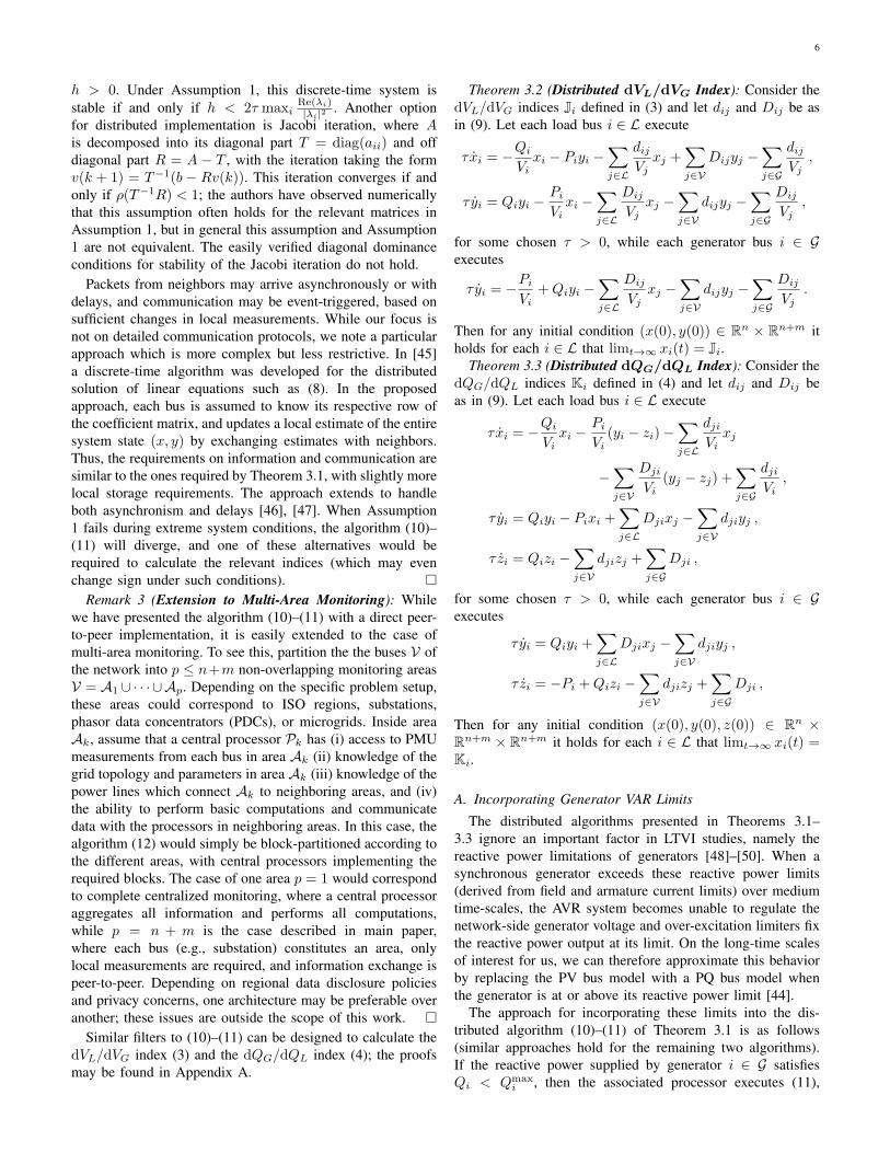
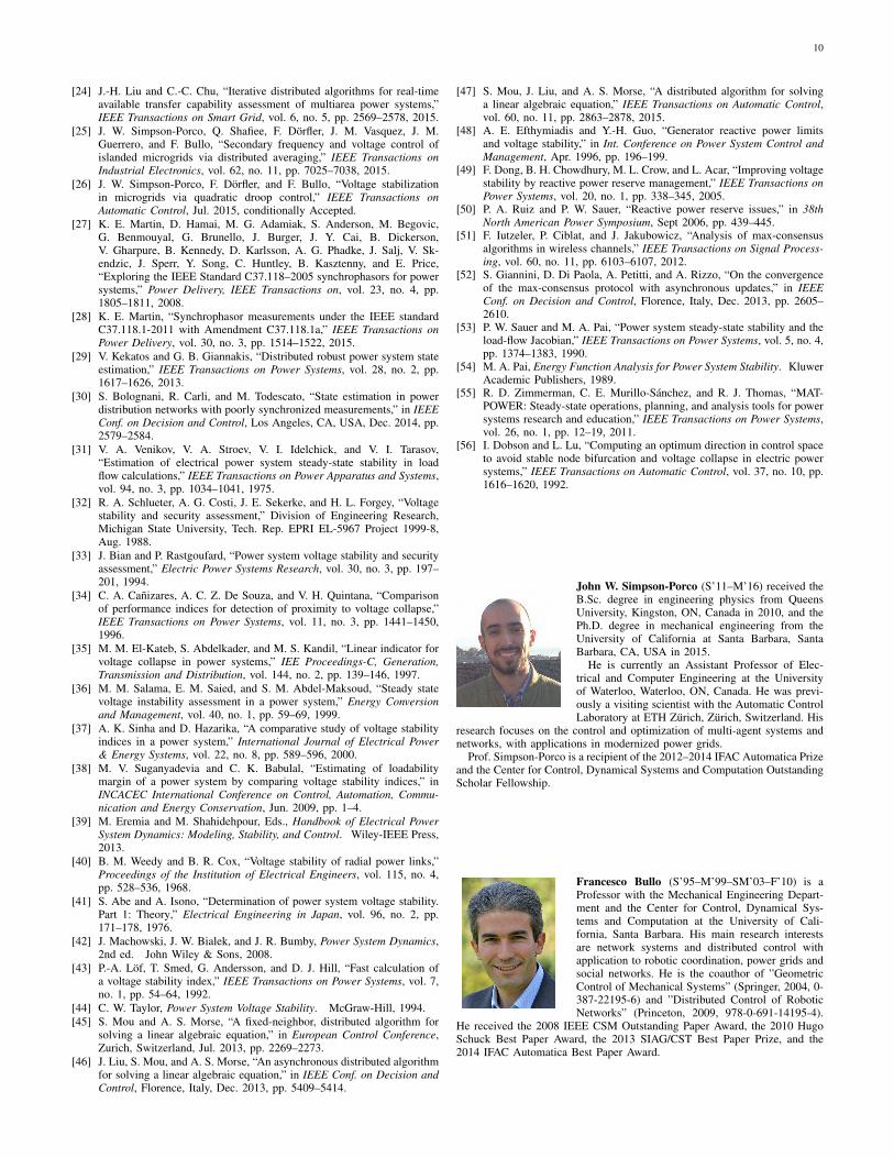
Figure 3 displays a close-up of the trace of xi(t) at bus 20

after the load is shed at t = 200s, along with the resulting

dynamics of the corresponding bus voltage V20(t). As our

algorithms use real-time measurements for computing the

sensitivity indices, transients experienced by the physical bus

variables also impact the filter estimates until convergence

occurs. As can be seen from Figure 3 however, transients in

physical variables tend to be damped significantly by the filter.

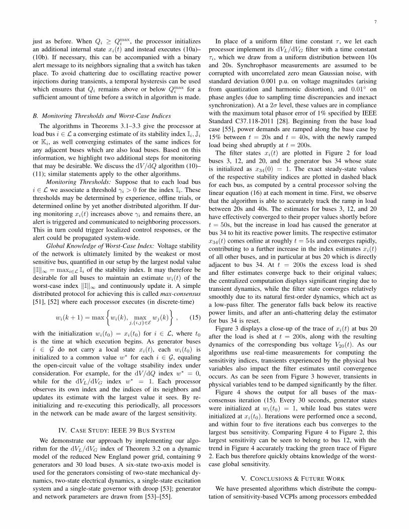
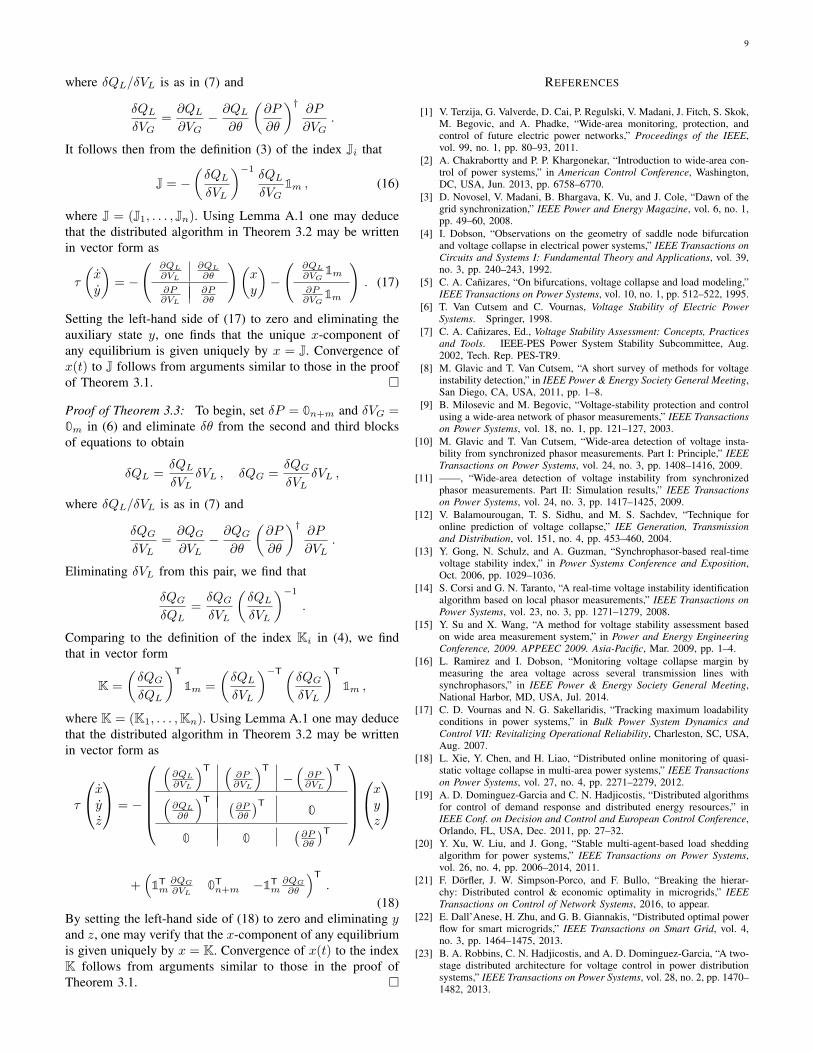
Figure 4 shows the output for all buses of the max-

consensus iteration (15). Every 30 seconds, generator states

were initialized at wi(t0) = 1, while load bus states were

initialized at xi(t0). Iterations were performed once a second,

and within four to five iterations each bus converges to the

largest bus sensitivity. Comparing Figure 4 to Figure 2, this

largest sensitivity can be seen to belong to bus 12, with the

trend in Figure 4 accurately tracking the green trace of Figure

2. Each bus therefore quickly obtains knowledge of the worst-

case global sensitivity.

V. CONCLUSIONS & FUTURE WORK

We have presented algorithms which distribute the compu-

tation of sensitivity-based VCPIs among processors embedded

8

0 50 100 150 200 250 3001

1.05

1.1

1.15

1.2

1.25

1.3dVL/dVGFilterEstim

atesxi(t)

Time (s)

Bus 3Bus 12Bus 20Bus 34

Fig. 2. Estimates xi(t) of the dVL/dVG indices for several buses. Blackdashed lines denote the exact index values for the respective buses, ascalculated in a centralized manner. Noise is omitted on the centralizedcalculation for clarity.

195 200 205 210 215 220 225 2300.85

0.9

0.95

1

1.05

1.1

1.15

1.2

FilterSta

teandVoltage(p

.u.)

Time (s)

x20V20

Fig. 3. Estimate x20(t) of the dVL/dVG index along with the bus voltageat bus 20 for t ∈ [195, 230]. The black dashed line denotes the exact indexvalue. Noise is omitted for clarity.

within a smart grid. Using PMU measurements and commu-

nication with adjacent buses, each bus is able to iteratively

calculate its exact sensitivity index. This exact computation is

achieved without the requirement of a central decision maker,

and we have illustrated the feasibility of the approach via

simulation study.

While in this work we have used a purely power flow-based

model to calculate sensitivities, an important extension is to

augment the power flow equations (1a)–(1b) with additional

equilibrium equations [6, Chapter 6] corresponding to gener-

ator, controller, limiter, and load dynamics. Moreover, steady-

state reactive power limits are typically functions of active

power injections. As these additional equilibrium equations

are typically not coupled between buses, designing analogous

distributed algorithms should be feasible, as inter-bus coupling

occurs only through the power flow equations. While we have

0 50 100 150 200 250 3001

1.05

1.1

1.15

1.2

1.25

1.3

Maxim

um

IndexEstim

atesw

i(t)

Time (s)

Fig. 4. Estimates wi(t) of maxi∈V xi(t) generated from the max-consensusalgorithm (15). The algorithm is reinitialized with the current value of xi(t)and re-executed every 30 seconds. Generator states are initialized from unity.

included a basic load-flow type model of generator reactive

power limits, more detailed models could be incorporated

which include limits based directly on field and armature cur-

rents. Future work will also concern relaxing the assumption

of full grid observability to partial observability by combining

the algorithms presented herein with distributed estimation.

Another key direction is the fusion of monitoring protocols

such as the one presented herein with automatic distributed

control and protection. It seems plausible that optimal control

directions in parameter space [56] can be computed and

executed in a distributed way, creating a self-healing grid.

APPENDIX A

TECHNICAL LEMMAS AND PROOFS

Lemma A.1 (Power Flow Jacobian): Let (θ, VL) ∈ Rn+m×Rn

>0 be a solution of the power flow equations (1a)–(1b), and

let dij and Dij be as in (9). When evaluated at at (θ, VL) the

partial derivatives of (1a)–(1b) are given (for j 6= i) by [42,

Sec. 3.5.1.1]

∂Pi

∂θi= −Qi + dii ,

∂Pi

∂θj= dij ,

Vi

∂Pi

∂Vi

= Pi +Dii , Vj

∂Pi

∂Vj

= Dij ,

Vi

∂Qi

∂Vi

= Qi + dii , Vj

∂Qi

∂Vj

= dij ,

∂Qi

∂θi= Pi −Dii ,

∂Qi

∂θj= −Dij .

Proof of Theorem 3.2: To begin, note that by setting δP =0n+m and δQL = 0n in (6) and eliminating δθ from the first

two blocks of equations, one obtains

0n =δQL

δVL

δVL +δQL

δVG

δVG ,

9

where δQL/δVL is as in (7) and

δQL

δVG

=∂QL

∂VG

−∂QL

∂θ

(

∂P

∂θ

)†∂P

∂VG

.

It follows then from the definition (3) of the index Ji that

J = −

(

δQL

δVL

)−1δQL

δVG

1m , (16)

where J = (J1, . . . , Jn). Using Lemma A.1 one may deduce

that the distributed algorithm in Theorem 3.2 may be written

in vector form as

τ

(

xy

)

= −

(

∂QL

∂VL

∂QL

∂θ

∂P∂VL

∂P∂θ

)

(

xy

)

−

(

∂QL

∂VG1m

∂P∂VG

1m

)

. (17)

Setting the left-hand side of (17) to zero and eliminating the

auxiliary state y, one finds that the unique x-component of

any equilibrium is given uniquely by x = J. Convergence of

x(t) to J follows from arguments similar to those in the proof

of Theorem 3.1. �

Proof of Theorem 3.3: To begin, set δP = 0n+m and δVG =0m in (6) and eliminate δθ from the second and third blocks

of equations to obtain

δQL =δQL

δVL

δVL , δQG =δQG

δVL

δVL ,

where δQL/δVL is as in (7) and

δQG

δVL

=∂QG

∂VL

−∂QG

∂θ

(

∂P

∂θ

)†∂P

∂VL

.

Eliminating δVL from this pair, we find that

δQG

δQL

=δQG

δVL

(

δQL

δVL

)−1

.

Comparing to the definition of the index Ki in (4), we find

that in vector form

K =

(

δQG

δQL

)T

1m =

(

δQL

δVL

)−T(

δQG

δVL

)T

1m ,

where K = (K1, . . . ,Kn). Using Lemma A.1 one may deduce

that the distributed algorithm in Theorem 3.2 may be written

in vector form as

τ

xyz

= −

(

∂QL

∂VL

)T (

∂P∂VL

)T

−(

∂P∂VL

)T

(

∂QL

∂θ

)T(

∂P∂θ

)T

0

0 0(

∂P∂θ

)T

xyz

+(

1T

m∂QG

∂VL0T

n+m −1T

m∂QG

∂θ

)T

.

(18)

By setting the left-hand side of (18) to zero and eliminating yand z, one may verify that the x-component of any equilibrium

is given uniquely by x = K. Convergence of x(t) to the index

K follows from arguments similar to those in the proof of

Theorem 3.1. �

REFERENCES

[1] V. Terzija, G. Valverde, D. Cai, P. Regulski, V. Madani, J. Fitch, S. Skok,M. Begovic, and A. Phadke, “Wide-area monitoring, protection, andcontrol of future electric power networks,” Proceedings of the IEEE,vol. 99, no. 1, pp. 80–93, 2011.

[2] A. Chakrabortty and P. P. Khargonekar, “Introduction to wide-area con-trol of power systems,” in American Control Conference, Washington,DC, USA, Jun. 2013, pp. 6758–6770.

[3] D. Novosel, V. Madani, B. Bhargava, K. Vu, and J. Cole, “Dawn of thegrid synchronization,” IEEE Power and Energy Magazine, vol. 6, no. 1,pp. 49–60, 2008.

[4] I. Dobson, “Observations on the geometry of saddle node bifurcationand voltage collapse in electrical power systems,” IEEE Transactions on

Circuits and Systems I: Fundamental Theory and Applications, vol. 39,no. 3, pp. 240–243, 1992.

[5] C. A. Canizares, “On bifurcations, voltage collapse and load modeling,”IEEE Transactions on Power Systems, vol. 10, no. 1, pp. 512–522, 1995.

[6] T. Van Cutsem and C. Vournas, Voltage Stability of Electric Power

Systems. Springer, 1998.

[7] C. A. Canizares, Ed., Voltage Stability Assessment: Concepts, Practices

and Tools. IEEE-PES Power System Stability Subcommittee, Aug.2002, Tech. Rep. PES-TR9.

[8] M. Glavic and T. Van Cutsem, “A short survey of methods for voltageinstability detection,” in IEEE Power & Energy Society General Meeting,San Diego, CA, USA, 2011, pp. 1–8.

[9] B. Milosevic and M. Begovic, “Voltage-stability protection and controlusing a wide-area network of phasor measurements,” IEEE Transactions

on Power Systems, vol. 18, no. 1, pp. 121–127, 2003.

[10] M. Glavic and T. Van Cutsem, “Wide-area detection of voltage insta-bility from synchronized phasor measurements. Part I: Principle,” IEEE

Transactions on Power Systems, vol. 24, no. 3, pp. 1408–1416, 2009.

[11] ——, “Wide-area detection of voltage instability from synchronizedphasor measurements. Part II: Simulation results,” IEEE Transactions

on Power Systems, vol. 24, no. 3, pp. 1417–1425, 2009.

[12] V. Balamourougan, T. S. Sidhu, and M. S. Sachdev, “Technique foronline prediction of voltage collapse,” IEE Generation, Transmission

and Distribution, vol. 151, no. 4, pp. 453–460, 2004.

[13] Y. Gong, N. Schulz, and A. Guzman, “Synchrophasor-based real-timevoltage stability index,” in Power Systems Conference and Exposition,Oct. 2006, pp. 1029–1036.

[14] S. Corsi and G. N. Taranto, “A real-time voltage instability identificationalgorithm based on local phasor measurements,” IEEE Transactions on

Power Systems, vol. 23, no. 3, pp. 1271–1279, 2008.

[15] Y. Su and X. Wang, “A method for voltage stability assessment basedon wide area measurement system,” in Power and Energy Engineering

Conference, 2009. APPEEC 2009. Asia-Pacific, Mar. 2009, pp. 1–4.

[16] L. Ramirez and I. Dobson, “Monitoring voltage collapse margin bymeasuring the area voltage across several transmission lines withsynchrophasors,” in IEEE Power & Energy Society General Meeting,National Harbor, MD, USA, Jul. 2014.

[17] C. D. Vournas and N. G. Sakellaridis, “Tracking maximum loadabilityconditions in power systems,” in Bulk Power System Dynamics and

Control VII: Revitalizing Operational Reliability, Charleston, SC, USA,Aug. 2007.

[18] L. Xie, Y. Chen, and H. Liao, “Distributed online monitoring of quasi-static voltage collapse in multi-area power systems,” IEEE Transactions

on Power Systems, vol. 27, no. 4, pp. 2271–2279, 2012.

[19] A. D. Dominguez-Garcia and C. N. Hadjicostis, “Distributed algorithmsfor control of demand response and distributed energy resources,” inIEEE Conf. on Decision and Control and European Control Conference,Orlando, FL, USA, Dec. 2011, pp. 27–32.

[20] Y. Xu, W. Liu, and J. Gong, “Stable multi-agent-based load sheddingalgorithm for power systems,” IEEE Transactions on Power Systems,vol. 26, no. 4, pp. 2006–2014, 2011.

[21] F. Dorfler, J. W. Simpson-Porco, and F. Bullo, “Breaking the hierar-chy: Distributed control & economic optimality in microgrids,” IEEE

Transactions on Control of Network Systems, 2016, to appear.

[22] E. Dall’Anese, H. Zhu, and G. B. Giannakis, “Distributed optimal powerflow for smart microgrids,” IEEE Transactions on Smart Grid, vol. 4,no. 3, pp. 1464–1475, 2013.

[23] B. A. Robbins, C. N. Hadjicostis, and A. D. Dominguez-Garcia, “A two-stage distributed architecture for voltage control in power distributionsystems,” IEEE Transactions on Power Systems, vol. 28, no. 2, pp. 1470–1482, 2013.

10

[24] J.-H. Liu and C.-C. Chu, “Iterative distributed algorithms for real-timeavailable transfer capability assessment of multiarea power systems,”IEEE Transactions on Smart Grid, vol. 6, no. 5, pp. 2569–2578, 2015.

[25] J. W. Simpson-Porco, Q. Shafiee, F. Dorfler, J. M. Vasquez, J. M.Guerrero, and F. Bullo, “Secondary frequency and voltage control ofislanded microgrids via distributed averaging,” IEEE Transactions on

Industrial Electronics, vol. 62, no. 11, pp. 7025–7038, 2015.

[26] J. W. Simpson-Porco, F. Dorfler, and F. Bullo, “Voltage stabilizationin microgrids via quadratic droop control,” IEEE Transactions on

Automatic Control, Jul. 2015, conditionally Accepted.

[27] K. E. Martin, D. Hamai, M. G. Adamiak, S. Anderson, M. Begovic,G. Benmouyal, G. Brunello, J. Burger, J. Y. Cai, B. Dickerson,V. Gharpure, B. Kennedy, D. Karlsson, A. G. Phadke, J. Salj, V. Sk-endzic, J. Sperr, Y. Song, C. Huntley, B. Kasztenny, and E. Price,“Exploring the IEEE Standard C37.118–2005 synchrophasors for powersystems,” Power Delivery, IEEE Transactions on, vol. 23, no. 4, pp.1805–1811, 2008.

[28] K. E. Martin, “Synchrophasor measurements under the IEEE standardC37.118.1-2011 with Amendment C37.118.1a,” IEEE Transactions on

Power Delivery, vol. 30, no. 3, pp. 1514–1522, 2015.

[29] V. Kekatos and G. B. Giannakis, “Distributed robust power system stateestimation,” IEEE Transactions on Power Systems, vol. 28, no. 2, pp.1617–1626, 2013.

[30] S. Bolognani, R. Carli, and M. Todescato, “State estimation in powerdistribution networks with poorly synchronized measurements,” in IEEE

Conf. on Decision and Control, Los Angeles, CA, USA, Dec. 2014, pp.2579–2584.

[31] V. A. Venikov, V. A. Stroev, V. I. Idelchick, and V. I. Tarasov,“Estimation of electrical power system steady-state stability in loadflow calculations,” IEEE Transactions on Power Apparatus and Systems,vol. 94, no. 3, pp. 1034–1041, 1975.

[32] R. A. Schlueter, A. G. Costi, J. E. Sekerke, and H. L. Forgey, “Voltagestability and security assessment,” Division of Engineering Research,Michigan State University, Tech. Rep. EPRI EL-5967 Project 1999-8,Aug. 1988.

[33] J. Bian and P. Rastgoufard, “Power system voltage stability and securityassessment,” Electric Power Systems Research, vol. 30, no. 3, pp. 197–201, 1994.

[34] C. A. Canizares, A. C. Z. De Souza, and V. H. Quintana, “Comparisonof performance indices for detection of proximity to voltage collapse,”IEEE Transactions on Power Systems, vol. 11, no. 3, pp. 1441–1450,1996.

[35] M. M. El-Kateb, S. Abdelkader, and M. S. Kandil, “Linear indicator forvoltage collapse in power systems,” IEE Proceedings-C, Generation,

Transmission and Distribution, vol. 144, no. 2, pp. 139–146, 1997.

[36] M. M. Salama, E. M. Saied, and S. M. Abdel-Maksoud, “Steady statevoltage instability assessment in a power system,” Energy Conversion

and Management, vol. 40, no. 1, pp. 59–69, 1999.

[37] A. K. Sinha and D. Hazarika, “A comparative study of voltage stabilityindices in a power system,” International Journal of Electrical Power

& Energy Systems, vol. 22, no. 8, pp. 589–596, 2000.

[38] M. V. Suganyadevia and C. K. Babulal, “Estimating of loadabilitymargin of a power system by comparing voltage stability indices,” inINCACEC International Conference on Control, Automation, Commu-

nication and Energy Conservation, Jun. 2009, pp. 1–4.

[39] M. Eremia and M. Shahidehpour, Eds., Handbook of Electrical Power

System Dynamics: Modeling, Stability, and Control. Wiley-IEEE Press,2013.

[40] B. M. Weedy and B. R. Cox, “Voltage stability of radial power links,”Proceedings of the Institution of Electrical Engineers, vol. 115, no. 4,pp. 528–536, 1968.

[41] S. Abe and A. Isono, “Determination of power system voltage stability.Part 1: Theory,” Electrical Engineering in Japan, vol. 96, no. 2, pp.171–178, 1976.

[42] J. Machowski, J. W. Bialek, and J. R. Bumby, Power System Dynamics,2nd ed. John Wiley & Sons, 2008.

[43] P.-A. Lof, T. Smed, G. Andersson, and D. J. Hill, “Fast calculation ofa voltage stability index,” IEEE Transactions on Power Systems, vol. 7,no. 1, pp. 54–64, 1992.

[44] C. W. Taylor, Power System Voltage Stability. McGraw-Hill, 1994.

[45] S. Mou and A. S. Morse, “A fixed-neighbor, distributed algorithm forsolving a linear algebraic equation,” in European Control Conference,Zurich, Switzerland, Jul. 2013, pp. 2269–2273.

[46] J. Liu, S. Mou, and A. S. Morse, “An asynchronous distributed algorithmfor solving a linear algebraic equation,” in IEEE Conf. on Decision and

Control, Florence, Italy, Dec. 2013, pp. 5409–5414.

[47] S. Mou, J. Liu, and A. S. Morse, “A distributed algorithm for solvinga linear algebraic equation,” IEEE Transactions on Automatic Control,vol. 60, no. 11, pp. 2863–2878, 2015.

[48] A. E. Efthymiadis and Y.-H. Guo, “Generator reactive power limitsand voltage stability,” in Int. Conference on Power System Control and

Management, Apr. 1996, pp. 196–199.[49] F. Dong, B. H. Chowdhury, M. L. Crow, and L. Acar, “Improving voltage

stability by reactive power reserve management,” IEEE Transactions on

Power Systems, vol. 20, no. 1, pp. 338–345, 2005.[50] P. A. Ruiz and P. W. Sauer, “Reactive power reserve issues,” in 38th

North American Power Symposium, Sept 2006, pp. 439–445.[51] F. Iutzeler, P. Ciblat, and J. Jakubowicz, “Analysis of max-consensus

algorithms in wireless channels,” IEEE Transactions on Signal Process-

ing, vol. 60, no. 11, pp. 6103–6107, 2012.[52] S. Giannini, D. Di Paola, A. Petitti, and A. Rizzo, “On the convergence

of the max-consensus protocol with asynchronous updates,” in IEEE

Conf. on Decision and Control, Florence, Italy, Dec. 2013, pp. 2605–2610.

[53] P. W. Sauer and M. A. Pai, “Power system steady-state stability and theload-flow Jacobian,” IEEE Transactions on Power Systems, vol. 5, no. 4,pp. 1374–1383, 1990.

[54] M. A. Pai, Energy Function Analysis for Power System Stability. KluwerAcademic Publishers, 1989.

[55] R. D. Zimmerman, C. E. Murillo-Sanchez, and R. J. Thomas, “MAT-POWER: Steady-state operations, planning, and analysis tools for powersystems research and education,” IEEE Transactions on Power Systems,vol. 26, no. 1, pp. 12–19, 2011.

[56] I. Dobson and L. Lu, “Computing an optimum direction in control spaceto avoid stable node bifurcation and voltage collapse in electric powersystems,” IEEE Transactions on Automatic Control, vol. 37, no. 10, pp.1616–1620, 1992.

John W. Simpson-Porco (S’11–M’16) received theB.Sc. degree in engineering physics from QueensUniversity, Kingston, ON, Canada in 2010, and thePh.D. degree in mechanical engineering from theUniversity of California at Santa Barbara, SantaBarbara, CA, USA in 2015.

He is currently an Assistant Professor of Elec-trical and Computer Engineering at the Universityof Waterloo, Waterloo, ON, Canada. He was previ-ously a visiting scientist with the Automatic ControlLaboratory at ETH Zurich, Zurich, Switzerland. His

research focuses on the control and optimization of multi-agent systems andnetworks, with applications in modernized power grids.

Prof. Simpson-Porco is a recipient of the 2012–2014 IFAC Automatica Prizeand the Center for Control, Dynamical Systems and Computation OutstandingScholar Fellowship.

Francesco Bullo (S’95–M’99–SM’03–F’10) is aProfessor with the Mechanical Engineering Depart-ment and the Center for Control, Dynamical Sys-tems and Computation at the University of Cali-fornia, Santa Barbara. His main research interestsare network systems and distributed control withapplication to robotic coordination, power grids andsocial networks. He is the coauthor of ”GeometricControl of Mechanical Systems” (Springer, 2004, 0-387-22195-6) and ”Distributed Control of RoboticNetworks” (Princeton, 2009, 978-0-691-14195-4).

He received the 2008 IEEE CSM Outstanding Paper Award, the 2010 HugoSchuck Best Paper Award, the 2013 SIAG/CST Best Paper Prize, and the2014 IFAC Automatica Best Paper Award.