Understanding LCA results variability: developing global sensitivity analysis with Sobol indices. A first application to photovoltaic systems

UNDERSTANDING LCA RESULTS VARIABILITY: DEVELOPING

GLOBAL SENSITIVITY ANALYSIS WITH SOBOL INDICES. A FIRST

APPLICATION TO PHOTOVOLTAIC SYSTEMS.

Pierryves Padey (1),(2), Didier Beloin-Saint-Pierre (2), Robin Girard (2), Denis Le-

Boulch (1), Isabelle Blanc (2)

(1) EDF R&D, Les Renardières 77818 Moret sur Loing Cedex, France

[email protected]

(2) MINES ParisTech, 1, rue Claude Daunesse, F-06904 Sophia Antipolis Cedex, France

Abstract

LCA has been extensively used in the last few years and a large number of studies have

been published in the literature. These studies show a great variability in results of

comparable systems. It somehow leads policy-makers to consider the LCA approach as an

inconclusive method. Some attempts have been developed to assess LCA results variability;

however, they remain mostly qualitative.

In this paper, a method based on Global Sensitivity Analysis (GSA) is presented in order to

understand the origin of results variability. A general variance decomposition based on the

Sobol indices is applied to quantify the influence of input parameters on the environmental

answer.

A preliminary study is done by using this GSA on a large set of integrated photovoltaic

systems greenhouse gas (GHG) performances. We identify that the irradiation parameter has

the biggest influence on those GHG performances. The other parameters such as lifetime or

performance ratio have been identified as having a smaller but significant influence on the

GHG results variability. The GHG performances range from 24 to 230 g CO2eq/kWh with

75% of the performance ranging from 23.8 to 93.5g CO2eq/kWh.

Keywords:

Sobol indices, variability, GHG performance, photovoltaic, GSA.

hal-0

0785

068,

ver

sion

1 -

5 Fe

b 20

13Author manuscript, published in "International Symposium on Life Cycle ssessment and Construction Civil engineering and

buildings, Nantes : France (2012)"

Page 1

1. INTRODUCTION

Life Cycle Assessment (LCA) is nowadays considered as one of the main relevant tool to

study a product or system environmental impacts. Therefore, LCA has been widely used in

order to assess the environmental impacts for a panorama of systems. The result is a large

quantity of LCA studies presenting a high variability in impacts results for comparable

systems. An IPCC report [1] clearly shows this situation for different sources of electricity

production over a large set of publications. In this report, the CO2 equivalent emissions for

photovoltaic (PV) electricity generation range between 5 and 217 g CO2eq/kWh. This high

variability tends to complicate the work of decision makers. We propose a method which aims

at explaining such variability in response to this situation.

Recently, the LCA research community initiated new methods; defined as meta-analysis,

to get a comprehensive panorama of systems environmental impacts [2],[3],[4]. These meta-

analyses aim at synthesizing and identifying the main sources of results‟ variability [3].

Understanding LCA variability requires the definition of its types and sources. Different

studies [5], [6] underline that defining that kind of information will improve the LCA method

reliability. Moreover, a selection of studies [7] has identified the possibility of explaining a

large proportion of environmental impacts variability with a limited number of parameters.

Sensitivity analyses have been identified as a necessary tool to improve the LCA results

representativeness [6] by quantifying the influence of input parameters on a system‟s environmental performances. However, when dealing with environmental impact assessment,

most sensitivity analyses remain at a local level as they evaluate the variation of the input

parameters one factor at a time [8]. This approach only partially reflects the LCA results

variability, because it does not consider the full range of input parameters interval, as well as

the combined variability and their probability distribution [8]. A statistical tool named Global

Sensitivity analyses (GSA), by opposition to the traditional local sensitivity analyses, exists

but only few studies [9][10] have proposed this systematic and generic method to identify the

most environmentally influential parameters for LCAs.

This paper aims at presenting a generic methodology that can explain part of the LCA‟s

results variability through input parameter variability assessment. The methodology we

propose relies on the study of different variability sources for electricity generation systems

through GSA. The GSA is performed through the computation of Sobol indices that are built

upon general variance decomposition [11]. This methodology is applied to a large sample of

building integrated PV electricity LCAs as a first example.

hal-0

0785

068,

ver

sion

1 -

5 Fe

b 20

13

Page 2

2. PROBLEMATIC

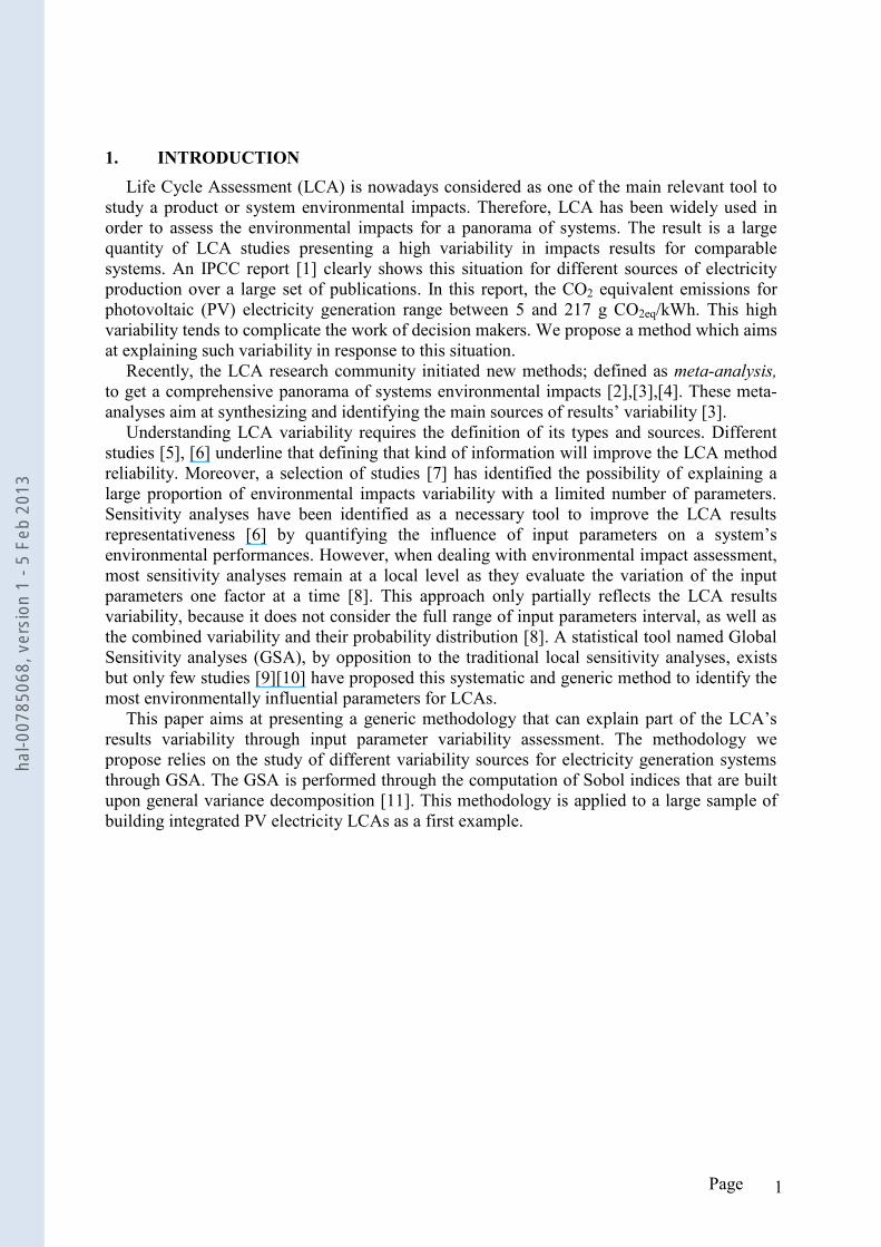
The LCA modeling process can be summarized as in Figure 1:

Figure 1 : Representation of the LCA model

Each stage of a LCA implies variability and uncertainty. Björklund [5] proposed to classify

these different sources; we will focus on the data inaccuracy (the quantifications of all input

parameters are dependant of measurements or data given by experts), the model uncertainty

(the model of the studied system for the LCA calculations is a simplified representation of the

reality), the uncertainty due to choice (the LCA practitioners need to make choices during the

modeling phase such as allocation rules, system boundaries, choice of average data…), the spatial variability (a renewable energy system, for example photovoltaic performance is

strongly dependant of its geo-localization) and the epistemological uncertainty (due to lack of

knowledge on system‟s behavior, such as the system‟s lifetime estimation). These aspects and limitations are known and accepted by LCA practitioners. However,

their transparent descriptions are limited in the literature.

This issue is a sensitive debated subject when modeling electricity generation systems. The

fast developments of renewable energy technologies and incentives policies require a clear

vision of renewable energies environmental impacts panorama. The IPCC [1] has made a

literature review of the GHG emissions for electricity generation systems which clearly shows

this problematic (see figure 2). This literature review has been based on different criterions

such as assumption transparency and temporal representativeness (the LCAs selected in the

IPCC review had to correspond to an up-to-date technology or to be representative of a near

future).

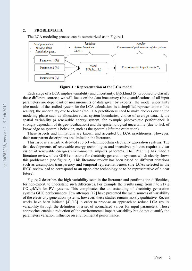
Figure 2 describes the high variability seen in the literature and confirms the difficulties,

for non-expert, to understand such differences. For example the results range from 5 to 217 g

CO2eq/kWh for PV systems. This complicates the understanding of electricity generation

systems GHG performances. Few attempts [12] have presented the main sources of variability

of the electricity generation systems; however, these studies remain mostly qualitative. Recent

works have been initiated [4],[13] in order to propose an approach to reduce LCA results

variability through the definition of a set of normalized values for input parameters. Those

approaches enable a reduction of the environmental impact variability but do not quantify the

parameters variation influence on environmental performance.

hal-0

0785

068,

ver

sion

1 -

5 Fe

b 20

13

Page 3

Figure 2 : GHG variability for electricity generation systems from IPCC graph [1]

Sensitivity analyses (SA) are approaches allowing investigating the results variability from

inputs parameters [14]. They are defined as the study of relationships between information

flowing in and out of models [9]. Thereby, performing SA enables a better understanding of

results variability.

Sensitivity analyses are not always used in LCA and as an alternative only best and worst

case scenarios are considered. The commonly used sensitivity analysis (SA) in LCA, named

local sensitivity analysis, does not give access to distributions of environmental impact results

and does not quantify the full influence of input parameter on the environmental answer. The

commonly used SA in LCA is defined as a local study where parameters vary inside an

interval around a nominal value. Other particular case of local sensitivity analyses are used in

LCA, where one factor is varied and the others are held constant (one-factor-at-a-time

approach OAT, [8]) however, this approach does not consider the possible interaction

between parameters.

To overcome these limitations (no probability distribution, no consideration of interaction and

local analysis only) another type of sensitivity analysis technique called Global Sensitivity

Analysis (GSA), by opposition to local SA, is of strong interest. GSA enables the

quantification of input parameters influence on the variance of output performance for

nonlinear and non monotonic model, by a decomposition of output total variance [15] [16].

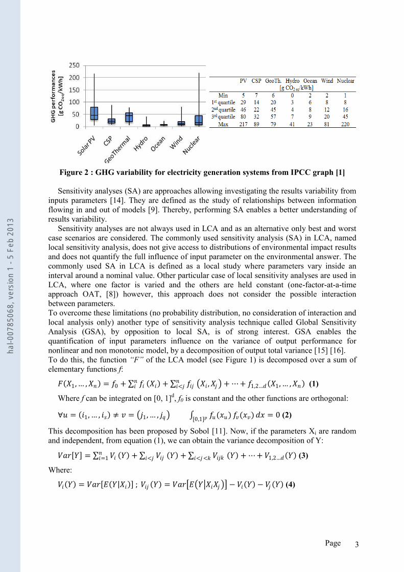
To do this, the function “F” of the LCA model (see Figure 1) is decomposed over a sum of

elementary functions f: ܨሺ1,ǥ ,ሻ = 0 + σ ሺ ሻ+ σ < ൫ , ൯ + +ڮ 1,2ǥሺ 1,ǥ ,ሻ (1)

Where f can be integrated on [0, 1]d, f0 is constant and the other functions are orthogonal: ݑ = ሺ1,ǥ , ሻݏ ݒ = ൫1,ǥ , ൯ݍ (ݑݔ)ݑ

[0,1] ݔ(ݒݔ)ݒ = 0 (2)

This decomposition has been proposed by Sobol [11]. Now, if the parameters Xi are random

and independent, from equation (1), we can obtain the variance decomposition of Y: ݎሾሿ = σ =1 ሺሻ + σ < ሺሻ + σ << ሺሻ + +ڮ 1,2ǥሺሻ (3)

Where: ሺሻ = ሺȁܧሾݎ ሻሿ ; ሺሻ = ൫หܧݎ ൯൧ െ ሺሻ െ ሺሻ (4)

hal-0

0785

068,

ver

sion

1 -

5 Fe

b 20

13

Page 4

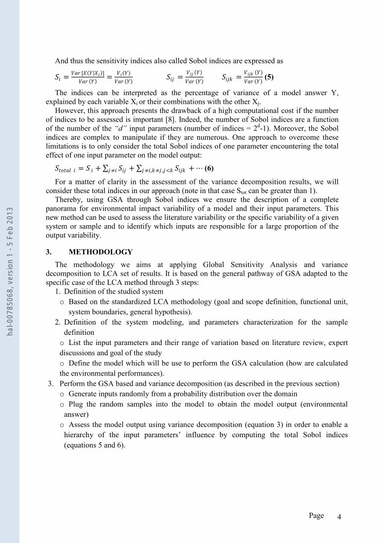
And thus the sensitivity indices also called Sobol indices are expressed as

=ݎ ݎ[ሺȁሻܧ] ሺሻ =

ሺሻݎ ሺሻ = ሺሻݎ ሺሻ =

ሺሻݎ ሺሻ (5)

The indices can be interpreted as the percentage of variance of a model answer Y,

explained by each variable Xi or their combinations with the other Xj.

However, this approach presents the drawback of a high computational cost if the number

of indices to be assessed is important [8]. Indeed, the number of Sobol indices are a function

of the number of the “d” input parameters (number of indices = 2d-1). Moreover, the Sobol

indices are complex to manipulate if they are numerous. One approach to overcome these

limitations is to only consider the total Sobol indices of one parameter encountering the total

effect of one input parameter on the model output: ݐݐ = + σ + σ , ,< + (6) ڮ

For a matter of clarity in the assessment of the variance decomposition results, we will

consider these total indices in our approach (note in that case Stot can be greater than 1).

Thereby, using GSA through Sobol indices we ensure the description of a complete

panorama for environmental impact variability of a model and their input parameters. This

new method can be used to assess the literature variability or the specific variability of a given

system or sample and to identify which inputs are responsible for a large proportion of the

output variability.

3. METHODOLOGY

The methodology we aims at applying Global Sensitivity Analysis and variance

decomposition to LCA set of results. It is based on the general pathway of GSA adapted to the

specific case of the LCA method through 3 steps:

1. Definition of the studied system

o Based on the standardized LCA methodology (goal and scope definition, functional unit,

system boundaries, general hypothesis).

2. Definition of the system modeling, and parameters characterization for the sample

definition

o List the input parameters and their range of variation based on literature review, expert

discussions and goal of the study

o Define the model which will be use to perform the GSA calculation (how are calculated

the environmental performances).

3. Perform the GSA based and variance decomposition (as described in the previous section)

o Generate inputs randomly from a probability distribution over the domain

o Plug the random samples into the model to obtain the model output (environmental

answer)

o Assess the model output using variance decomposition (equation 3) in order to enable a

hierarchy of the input parameters‟ influence by computing the total Sobol indices

(equations 5 and 6).

hal-0

0785

068,

ver

sion

1 -

5 Fe

b 20

13

Page 5

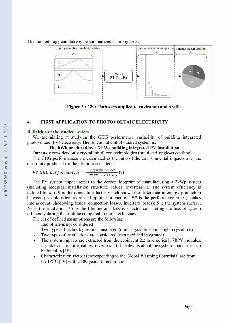
The methodology can thereby be summarized as in Figure 3:

Figure 3 : GSA Pathways applied to environmental profile

4. FIRST APPLICATION TO PHOTOVOLTAIC ELECTRICITY

Definition of the studied system

We are aiming at studying the GHG performance variability of building integrated

photovoltaic (PV) electricity. The functional unit of studied system is:

The kWh produced by a 3 kWp building integrated PV installation

Our study considers only crystalline silicon technologies (multi and single-crystalline).

The GHG performances are calculated as the ratio of the environmental impacts over the

electricity produced for the life time considered: ݏݎݎ ܩܪܩ = ݐݏݕݏ ߟݐܫ .. ݎݎܫ.. ݏݏ.ܮ. (7)

The PV system impact refers to the carbon footprint of manufacturing a 3kWp system

(including modules, installation structure, cables, inverters…). The system efficiency is

defined by さ, OR is the orientation factor which shows the difference in energy production

between possible orientations and optimal orientation; PR is the performance ratio (it takes

into account: shadowing losses, connection losses, inverters losses); S is the system surface,

Irr is the irradiation, LT is the lifetime and loss is a factor considering the loss of system

efficiency during the lifetime compared to initial efficiency.

The set of defined assumptions are the following:

- End of life is not considered

- Two types of technologies are considered (multi-crystalline and single-crystalline)

- Two types of installations are considered (mounted and integrated)

- The system impacts are extracted from the ecoinvent 2.2 inventories [17](PV modules,

installation structure, cables, inverters…). The details about the system boundaries can be found in [18]

- Characterization factors (corresponding to the Global Warming Potentials) are from

the IPCC [19] with a 100 years‟ time horizon

hal-0

0785

068,

ver

sion

1 -

5 Fe

b 20

13

Page 6

Characterization of the inputs parameters

The input parameter definitions, characterizations and distributions of our model are: Parameters Distribution Characterization

Peak Power [kW] Since the study is on residential, we fixed the value at 3kWp

System selection As described above, there are 2 types of technologies (single or multi-silicon) as well

as 2 types of installations structure (mounted or integrated). The system selection is

made with equiprobability distribution over these 4 technical choices.

System Impacts

[kg CO2 eq]

Module impacts (for both technologies and installation structures) are issued from

ecoinvent V2.2 [17]. In addition, we defined an uncertainty impact distribution

following a normal law centered on the ecoinvent values with a 15% relative

standard deviation This has been proposed in order to assess the influence of the

possible inventory uncertainty on the GHG performances

Irradiation [kWh/m2] Annual irradiation between 900 to 2200 kWh/m² with equiprobability distribution

Lifetime [years] In the literature, we observed lifetimes ranging between 20 and 30 years. We decided

to define the lifetime distribution as a normal law centered on 25 years with SD=2

Efficiency [%] The efficiency range and distribution for each studied technologies (multi and single

Si) have been estimated according to IEA PVPS work [20]. Therefore, the variability

due to the system selection as well as the efficiency variability for a same technology

are addressed. The range is between 0.10 to 0.16.

Orientation factor

[-]

The orientation factor has been defined as ranging between 0, 75 to 1. This represents

installation ranging from optimized to fully perpendicular to fully horizontal but it

can also represent installation directed in the western or eastern direction

Performance ratio

[-]

The efficiency range and distribution have been estimated according to IEA PVPS

work [20] ranging from 0.65 to 0.90

Surface [m2] The systems‟ surfaces have been calculated as a function of system efficiency in

order to keep the system peak power constant

Loss [%] Loss factor of 1% each year in production compared to year n-1 (estimation)

Table 1 Input parameters characterization for a GSA on residential PV electricity

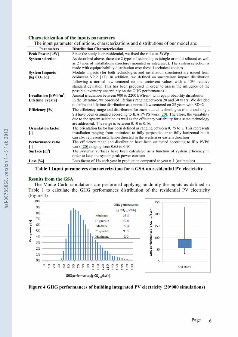
Results from the GSA

The Monte Carlo simulations are performed applying randomly the inputs as defined in

Table 1 to calculate the GHG performances distribution of the residential PV electricity

(Figure 4).

Figure 4 GHG performances of building integrated PV electricity (20‘000 simulations)

hal-0

0785

068,

ver

sion

1 -

5 Fe

b 20

13

Page 7

According to our sample definition on which we apply the Monte Carlo simulations, the

GHG performances vary from one order of magnitude between the minimum and maximum

values. The median, 1st and 3

rd quartiles values are below 100 g CO2eq/kWh. Compared to

IPCC literature survey [1], the coverage range of GHG performance is slighter higher.

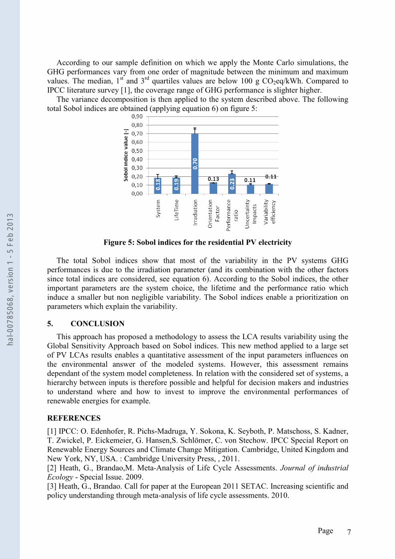
The variance decomposition is then applied to the system described above. The following

total Sobol indices are obtained (applying equation 6) on figure 5:

Figure 5: Sobol indices for the residential PV electricity

The total Sobol indices show that most of the variability in the PV systems GHG

performances is due to the irradiation parameter (and its combination with the other factors

since total indices are considered, see equation 6). According to the Sobol indices, the other

important parameters are the system choice, the lifetime and the performance ratio which

induce a smaller but non negligible variability. The Sobol indices enable a prioritization on

parameters which explain the variability.

5. CONCLUSION

This approach has proposed a methodology to assess the LCA results variability using the

Global Sensitivity Approach based on Sobol indices. This new method applied to a large set

of PV LCAs results enables a quantitative assessment of the input parameters influences on

the environmental answer of the modeled systems. However, this assessment remains

dependant of the system model completeness. In relation with the considered set of systems, a

hierarchy between inputs is therefore possible and helpful for decision makers and industries

to understand where and how to invest to improve the environmental performances of

renewable energies for example.

REFERENCES

[1] IPCC: O. Edenhofer, R. Pichs-Madruga, Y. Sokona, K. Seyboth, P. Matschoss, S. Kadner,

T. Zwickel, P. Eickemeier, G. Hansen,S. Schlömer, C. von Stechow. IPCC Special Report on

Renewable Energy Sources and Climate Change Mitigation. Cambridge, United Kingdom and

New York, NY, USA. : Cambridge University Press, , 2011.

[2] Heath, G., Brandao,M. Meta-Analysis of Life Cycle Assessments. Journal of industrial

Ecology - Special Issue. 2009.

[3] Heath, G., Brandao. Call for paper at the European 2011 SETAC. Increasing scientific and

policy understanding through meta-analysis of life cycle assessments. 2010.

hal-0

0785

068,

ver

sion

1 -

5 Fe

b 20

13

Page 8

[4] Plevin, R., Heath, G., Chul Kim, H., Sovacool, B. The American Center for Life Cycle

Assessment - LCA X Conference. Portland , 2010.

[5] Björklund, A. E. Survey of approaches to improve Reliability in LCA. The International

Journal of Life Cycle Assessment. pp. 64-72. Vol. 7, 2002.

[6] Reap, J., Roman, F., Duncan, S., Bras, B. A Survey of unreseolved problems in life cycle

assessment. Part 2: Impact Assessment and interpretation. The International Journal of Life

Cycle Assessment. pp. 374-388, 2008.

[7] Bala, A., Raugei, M., Benveniste, G. , Gazulla, C. and Fullana-i-Palmer, P. Simplified

tools for global warming potential evaluation: when „good enough‟ is best. The International

Journal of Life Cycle Assessment. pp. 489-498. Vol. 15, 2010

[8] Saltelli, A.,Ratto, M., Tarantola, S., Campolongo, F.,European Commission, Joint

Research Centre of Ispra. Sensitivity analysis practices: Strategies for model-based inference.

Reliability Engineering and System Safety. pp. 1109–1125, 2006.

[9] Tarantola S., Jesinghaus J., Puolamaa M. Saltelli et al., editors Sensitivity analysis. New

York : Wiley pp. 385–97, 2000.

[10] I. Kioutsioukis, S. Tarantola, A. Saltelli, and D. Gatelli, “Uncertainty and global sensitivity analysis of road transport emission estimates,” Atmospheric Environment, vol. 38,

no. 38, pp. 6609 – 6620, 2004,

[11] Sobol, I.M. Sensitivity estimates for non linear mathematical models. Mathematical

Modelling and Computational Experiments. pp. 407–414, 1993.

[12] Weisser, D. A guide to life-cycle greenhouse gas (GHG) emissions from electric supply

technologies. Energy. pp. 1543-1559. Vol. 32, 2007.

[13] Alsema E., Fraile D., Frischknecht R., Fthenakis V., Held M., Kim H.C., Pölz W.,

Raugei M., de Wild Scholten M., Methodology Guidelines on Life Cycle Assessment of

Photovoltaic Electricity, Subtask 20 "LCA", EA PVPS Task 12, 2009.

[14] Sustainability, European Comission - Joint Research Center - Insitute fo Environment

and. International Reference Life Cycle Data System (ILCD) Handbook - General Guide for

Life Cycle Assessment - Detailed guidance. First edition. s.l. : Publication Office of the

European Union, 2010.

[15] Iooss, B. Revue sur l‟analyse de sensibilité globale de modèles numériques. Journal de

la Société Française de Statistique. 2011.

[16] Jacques, J. Pratique de l‟analyse de sensibilité : comment évaluer l‟impact des entrées aléatoires sur la sortie d‟un modèle mathématique. Lille : s.n., 2011.

[17] ecoinvent. Database Version 2.2. 2010.

[18] Jungbluth N, "Life cycle assessment of crystalline photovoltaics in the swiss ecoinvent

database," Progress in Photovoltaics, vol. 13, pp. 429-446, 2005.

[19]Forster, P., V. Ramaswamy, P. Artaxo, T. Berntsen, R. Betts, D.W. Fahey, J. Haywood, J.

Lean, D.C. Lowe, G. Myhre, J. Nganga, R. Prinn, G. Raga, M. Schulz and R. Van Dorland,

2007: Changes in Atmospheric Constituents and in Radiative Forcing. In: Climate Change

2007: The Physical Science Basis. Contribution of Working Group I to the Fourth Assessment

Report of the Intergovernmental Panel on Climate Change [Solomon, S., D. Qin, M.

Manning, Z. Chen, M. Marquis, K.B. Averyt, M.Tignor and H.L. Miller (eds.)]. Cambridge

University Press, Cambridge, United Kingdom and New York, NY, USA. 2007

[20] Clavadetscher L and Nordmann T, " Cost and performance trends in grid-connected

photovoltaic systems and case studies" 2007, Report IEA PVPS T2-06, 2007.

hal-0

0785

068,

ver

sion

1 -

5 Fe

b 20

13