Distributed Compressive Sensing

arX

iv:0

901.

3403

v1 [

cs.I

T]

22

Jan

2009

Distributed Compressive Sensing

Dror Baron,1 Marco F. Duarte,2 Michael B. Wakin,3

Shriram Sarvotham,4 and Richard G. Baraniuk2 ∗

1Department of Electrical Engineering, Technion – Israel Institute of Technology, Haifa, Israel2Department of Electrical and Computer Engineering, Rice University, Houston, TX

3Division of Engineering, Colorado School of Mines, Golden, CO4Halliburton, Houston, TX

This paper is dedicated to the memory of Hyeokho Choi, our colleague, mentor, and friend.

Abstract

Compressive sensing is a signal acquisition framework based on the revelation that a small col-lection of linear projections of a sparse signal contains enough information for stable recovery.In this paper we introduce a new theory for distributed compressive sensing (DCS) that en-ables new distributed coding algorithms for multi-signal ensembles that exploit both intra- andinter-signal correlation structures. The DCS theory rests on a new concept that we term thejoint sparsity of a signal ensemble. Our theoretical contribution is to characterize the funda-mental performance limits of DCS recovery for jointly sparse signal ensembles in the noiselessmeasurement setting; our result connects single-signal, joint, and distributed (multi-encoder)compressive sensing. To demonstrate the efficacy of our framework and to show that additionalchallenges such as computational tractability can be addressed, we study in detail three examplemodels for jointly sparse signals. For these models, we develop practical algorithms for jointrecovery of multiple signals from incoherent projections. In two of our three models, the resultsare asymptotically best-possible, meaning that both the upper and lower bounds match theperformance of our practical algorithms. Moreover, simulations indicate that the asymptoticstake effect with just a moderate number of signals. DCS is immediately applicable to a rangeof problems in sensor arrays and networks.

Keywords: Compressive sensing, distributed source coding, sparsity, random projection, random matrix,

linear programming, array processing, sensor networks.

1 Introduction

A core tenet of signal processing and information theory is that signals, images, and other data oftencontain some type of structure that enables intelligent representation and processing. The notionof structure has been characterized and exploited in a variety of ways for a variety of purposes. Inthis paper, we focus on exploiting signal correlations for the purpose of compression.

∗This work was supported by the grants NSF CCF-0431150 and CCF-0728867, DARPA HR0011-08-1-0078,DARPA/ONR N66001-08-1-2065, ONR N00014-07-1-0936 and N00014-08-1-1112, AFOSR FA9550-07-1-0301, AROMURI W311NF-07-1-0185, and the Texas Instruments Leadership University Program. Preliminary versions of thiswork have appeared at the Allerton Conference on Communication, Control, and Computing [1], the Asilomar Con-ference on Signals, Systems and Computers [2], the Conference on Neural Information Processing Systems [3], andthe Workshop on Sensor, Signal and Information Processing [4].E-mail: [email protected], duarte, shri, [email protected], [email protected]; Web: dsp.rice.edu/cs

Current state-of-the-art compression algorithms employ a decorrelating transform such as anexact or approximate Karhunen-Loeve transform (KLT) to compact a correlated signal’s energyinto just a few essential coefficients [5–7]. Such transform coders exploit the fact that many signalshave a sparse representation in terms of some basis, meaning that a small number K of adaptivelychosen transform coefficients can be transmitted or stored rather than N ≫ K signal samples. Forexample, smooth signals are sparse in the Fourier basis, and piecewise smooth signals are sparsein a wavelet basis [8]; the commercial coding standards MP3 [9], JPEG [10], and JPEG2000 [11]directly exploit this sparsity.

1.1 Distributed source coding

While the theory and practice of compression have been well developed for individual signals,distributed sensing applications involve multiple signals, for which there has been less progress.Such settings are motivated by the proliferation of complex, multi-signal acquisition architectures,such as acoustic and RF sensor arrays, as well as sensor networks. These architectures sometimesinvolve battery-powered devices, which restrict the communication energy, and high aggregate datarates, limiting bandwidth availability; both factors make the reduction of communication critical.

Fortunately, since the sensors presumably observe related phenomena, the ensemble of signalsthey acquire can be expected to possess some joint structure, or inter-signal correlation, in additionto the intra-signal correlation within each individual sensor’s measurements. In such settings,distributed source coding that exploits both intra- and inter-signal correlations might allow thenetwork to save on the communication costs involved in exporting the ensemble of signals to thecollection point [12–15]. A number of distributed coding algorithms have been developed thatinvolve collaboration amongst the sensors [16–19]. Note, however, that any collaboration involvessome amount of inter-sensor communication overhead.

In the Slepian-Wolf framework for lossless distributed coding [12–15], the availability of corre-lated side information at the decoder (collection point) enables each sensor node to communicatelosslessly at its conditional entropy rate rather than at its individual entropy rate, as long as the sumrate exceeds the joint entropy rate. Slepian-Wolf coding has the distinct advantage that the sen-sors need not collaborate while encoding their measurements, which saves valuable communicationoverhead. Unfortunately, however, most existing coding algorithms [14, 15] exploit only inter-signalcorrelations and not intra-signal correlations. To date there has been only limited progress ondistributed coding of so-called “sources with memory.” The direct implementation for sources withmemory would require huge lookup tables [12]. Furthermore, approaches combining pre- or post-processing of the data to remove intra-signal correlations combined with Slepian-Wolf coding forthe inter-signal correlations appear to have limited applicability, because such processing wouldalter the data in a way that is unknown to other nodes. Finally, although recent papers [20–22]provide compression of spatially correlated sources with memory, the solution is specific to losslessdistributed compression and cannot be readily extended to lossy compression settings. We concludethat the design of constructive techniques for distributed coding of sources with both intra- andinter-signal correlation is a challenging problem with many potential applications.

1.2 Compressive sensing (CS)

A new framework for single-signal sensing and compression has developed under the rubric ofcompressive sensing (CS). CS builds on the work of Candes, Romberg, and Tao [23] and Donoho [24],who showed that if a signal has a sparse representation in one basis then it can be recovered from

2

a small number of projections onto a second basis that is incoherent with the first.1 CS relies ontractable recovery procedures that can provide exact recovery of a signal of length N and sparsityK, i.e., a signal that can be written as a sum of K basis functions from some known basis, whereK can be orders of magnitude less than N .

The implications of CS are promising for many applications, especially for sensing signals thathave a sparse representation in some basis. Instead of sampling a K-sparse signal N times, onlyM = O(K logN) incoherent measurements suffice, where K can be orders of magnitude less thanN . Moreover, the M measurements need not be manipulated in any way before being transmitted,except possibly for some quantization. Finally, independent and identically distributed (i.i.d.)Gaussian or Bernoulli/Rademacher (random ±1) vectors provide a useful universal basis that isincoherent with all others. Hence, when using a random basis, CS is universal in the sense that thesensor can apply the same measurement mechanism no matter what basis sparsifies the signal [27].

While powerful, the CS theory at present is designed mainly to exploit intra-signal structuresat a single sensor. In a multi-sensor setting, one can naively obtain separate measurements fromeach signal and recover them separately. However, it is possible to obtain measurements that eachdepend on all signals in the ensemble by having sensors collaborate with each other in order tocombine all of their measurements; we term this process a joint measurement setting. In fact, initialwork in CS for multi-sensor settings used standard CS with joint measurement and recovery schemesthat exploit inter-signal correlations [28–32]. However, by recovering sequential time instances ofthe sensed data individually, these schemes ignore intra-signal correlations.

1.3 Distributed compressive sensing (DCS)

In this paper we introduce a new theory for distributed compressive sensing (DCS) to enable newdistributed coding algorithms that exploit both intra- and inter-signal correlation structures. Ina typical DCS scenario, a number of sensors measure signals that are each individually sparse insome basis and also correlated from sensor to sensor. Each sensor separately encodes its signalby projecting it onto another, incoherent basis (such as a random one) and then transmits just afew of the resulting coefficients to a single collection point. Unlike the joint measurement settingdescribed in Section 1.2, DCS requires no collaboration between the sensors during signal acquisi-tion. Nevertheless, we are able to exploit the inter-signal correlation by using all of the obtainedmeasurements to recover all the signals simultaneously. Under the right conditions, a decoder atthe collection point can recover each of the signals precisely.

The DCS theory rests on a concept that we term the joint sparsity — the sparsity of theentire signal ensemble. The joint sparsity is often smaller than the aggregate over individual signalsparsities. Therefore, DCS offers a reduction in the number of measurements, in a manner analogousto the rate reduction offered by the Slepian-Wolf framework [13]. Unlike the single-signal definitionof sparsity, however, there are numerous plausible ways in which joint sparsity could be defined. Inthis paper, we first provide a general framework for joint sparsity using algebraic formulations basedon a graphical model. Using this framework, we derive bounds for the number of measurementsnecessary for recovery under a given signal ensemble model. Similar to Slepian-Wolf coding [13], thenumber of measurements required for each sensor must account for the minimal features unique tothat sensor, while at the same time features that appear among multiple sensors must be amortizedover the group. Our bounds are dependent on the dimensionality of the subspaces in which eachgroup of signals reside; they afford a reduction in the number of measurements that we quantifythrough the notions of joint and conditional sparsity, which are conceptually related to joint and

1Roughly speaking, incoherence means that no element of one basis has a sparse representation in terms of theother basis. This notion has a variety of formalizations in the CS literature [24–26].

3

conditional entropies. The common thread is that dimensionality and entropy both quantify thevolume that the measurement and coding rates must cover. Our results are also applicable to caseswhere the signal ensembles are measured jointly, as well as to the single-signal case.

While our general framework does not by design provide insights for computationally efficientrecovery, we also provide interesting models for joint sparsity where our results carry through fromthe general framework to realistic settings with low-complexity algorithms. In the first model,each signal is itself sparse, and so we could use CS to separately encode and decode each signal.However, there also exists a framework wherein a joint sparsity model for the ensemble uses fewertotal coefficients. In the second model, all signals share the locations of the nonzero coefficients.In the third model, no signal is itself sparse, yet there still exists a joint sparsity among the signalsthat allows recovery from significantly fewer than N measurements per sensor. For each modelwe propose tractable algorithms for joint signal recovery, followed by theoretical and empiricalcharacterizations of the number of measurements per sensor required for accurate recovery. Weshow that, under these models, joint signal recovery can recover signal ensembles from significantlyfewer measurements than would be required to recover each signal individually. In fact, for two ofour three models we obtain best-possible performance that could not be bettered by an oracle thatknew the the indices of the nonzero entries of the signals.

This paper focuses primarily on the basic task of reducing the number of measurements forrecovery of a signal ensemble in order to reduce the communication cost of source coding thatensemble. Our emphasis is on noiseless measurements of strictly sparse signals, where the optimalrecovery relies on ℓ0-norm optimization,2 which is computationally intractable. In practical settings,additional criteria may be relevant for measuring performance. For example, the measurements willtypically be real numbers that must be quantized, which gradually degrades the recovery quality asthe quantization becomes coarser [33, 34]. Characterizing DCS in light of practical considerationssuch as rate-distortion tradeoffs, power consumption in sensor networks, etc., are topics of futureresearch [31, 32].

1.4 Paper organization

Section 2 overviews the single-signal CS theories and provides a new result on CS recovery. Whilesome readers may be familiar with this material, we include it to make the paper self-contained.Section 3 introduces our general framework for joint sparsity models and proposes three examplemodels for joint sparsity. We provide our detailed analysis for the general framework in Section 4;we then address the three models in Section 5. We close the paper with a discussion and conclusionsin Section 6. Several appendices contain the proofs.

2 Compressive Sensing Background

2.1 Transform coding

Consider a real-valued signal3 x ∈ RN indexed as x(n), n ∈ 1, 2, . . . , N. Suppose that the basis

Ψ = [ψ1, . . . , ψN ] provides a K-sparse representation of x; that is,

x =N∑

n=1

ϑ(n)ψn =K∑

k=1

ϑ(nk)ψnk, (1)

2The ℓ0 “norm” ‖x‖0 merely counts the number of nonzero entries in the vector x.3Without loss of generality, we will focus on one-dimensional signals (vectors) for notational simplicity; the exten-

sion to multi-dimensional signal, e.g., images, is straightforward.

4

where x is a linear combination of K vectors chosen from Ψ, nk are the indices of those vectors,and ϑ(n) are the coefficients; the concept is extendable to tight frames [8]. Alternatively, we canwrite in matrix notation x = Ψϑ, where x is an N × 1 column vector, the sparse basis matrix Ψis N ×N with the basis vectors ψn as columns, and ϑ is an N × 1 column vector with K nonzeroelements. Using ‖ · ‖p to denote the ℓp norm, we can write that ‖ϑ‖0 = K; we can also write theset of nonzero indices Ω ⊆ 1, . . . , N, with |Ω| = K. Various expansions, including wavelets [8],Gabor bases [8], curvelets [35], etc., are widely used for representation and compression of naturalsignals, images, and other data.

The standard procedure for compressing sparse and nearly-sparse signals, known as transformcoding, is to (i) acquire the full N -sample signal x; (ii) compute the complete set of transformcoefficients ϑ(n); (iii) locate the K largest, significant coefficients and discard the (many) smallcoefficients; (iv) encode the values and locations of the largest coefficients. This procedure has threeinherent inefficiencies: First, for a high-dimensional signal, we must start with a large number ofsamples N . Second, the encoder must compute all of the N transform coefficients ϑ(n), eventhough it will discard all but K of them. Third, the encoder must encode the locations of the largecoefficients, which requires increasing the coding rate since the locations change with each signal.

We will focus our theoretical development on exactly K-sparse signals and defer discussion ofthe more general situation of compressible signals where the coefficients decay rapidly with a powerlaw but not to zero. Section 6 contains additional discussion on real-world compressible signals,and [36] presents simulation results.

2.2 Incoherent projections

These inefficiencies raise a simple question: For a given signal, is it possible to directly estimatethe set of large ϑ(n)’s that will not be discarded? While this seems improbable, Candes, Romberg,and Tao [23, 25] and Donoho [24] have shown that a reduced set of projections can contain enoughinformation to recover sparse signals. A framework to acquire sparse signals, often referred to ascompressive sensing (CS) [37], has emerged that builds on this principle.

In CS, we do not measure or encode the K significant ϑ(n) directly. Rather, we measureand encode M < N projections y(m) = 〈x, φT

m〉 of the signal onto a second set of functionsφm,m = 1, 2, . . . ,M , where φT

m denotes the transpose of φm and 〈·, ·〉 denotes the inner product.In matrix notation, we measure y = Φx, where y is an M × 1 column vector and the measurementmatrix Φ is M ×N with each row a measurement vector φm. Since M < N , recovery of the signalx from the measurements y is ill-posed in general; however the additional assumption of signalsparsity makes recovery possible and practical.

The CS theory tells us that when certain conditions hold, namely that the basis ψn cannotsparsely represent the vectors φm (a condition known as incoherence [24–26]) and the numberof measurements M is large enough (proportional to K), then it is indeed possible to recover theset of large ϑ(n) (and thus the signal x) from the set of measurements y(m) [24, 25]. Thisincoherence property holds for many pairs of bases, including for example, delta spikes and the sinewaves of a Fourier basis, or the Fourier basis and wavelets. Signals that are sparsely representedin frames or unions of bases can be recovered from incoherent measurements in the same fashion.Significantly, this incoherence also holds with high probability between any arbitrary fixed basisor frame and a randomly generated one. In the sequel, we will focus our analysis to such randommeasurement procedures.

5

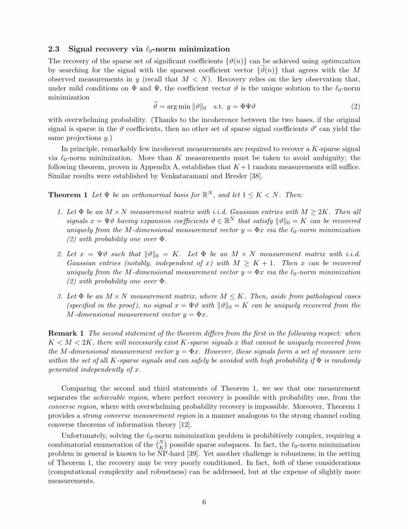
2.3 Signal recovery via ℓ0-norm minimization

The recovery of the sparse set of significant coefficients ϑ(n) can be achieved using optimizationby searching for the signal with the sparsest coefficient vector ϑ(n) that agrees with the Mobserved measurements in y (recall that M < N). Recovery relies on the key observation that,under mild conditions on Φ and Ψ, the coefficient vector ϑ is the unique solution to the ℓ0-normminimization

ϑ = arg min ‖ϑ‖0 s.t. y = ΦΨϑ (2)

with overwhelming probability. (Thanks to the incoherence between the two bases, if the originalsignal is sparse in the ϑ coefficients, then no other set of sparse signal coefficients ϑ′ can yield thesame projections y.)

In principle, remarkably few incoherent measurements are required to recover a K-sparse signalvia ℓ0-norm minimization. More than K measurements must be taken to avoid ambiguity; thefollowing theorem, proven in Appendix A, establishes that K+1 random measurements will suffice.Similar results were established by Venkataramani and Bresler [38].

Theorem 1 Let Ψ be an orthonormal basis for RN , and let 1 ≤ K < N . Then:

1. Let Φ be an M ×N measurement matrix with i.i.d. Gaussian entries with M ≥ 2K. Then allsignals x = Ψϑ having expansion coefficients ϑ ∈ R

N that satisfy ‖ϑ‖0 = K can be recovereduniquely from the M -dimensional measurement vector y = Φx via the ℓ0-norm minimization(2) with probability one over Φ.

2. Let x = Ψϑ such that ‖ϑ‖0 = K. Let Φ be an M × N measurement matrix with i.i.d.Gaussian entries (notably, independent of x) with M ≥ K + 1. Then x can be recovereduniquely from the M -dimensional measurement vector y = Φx via the ℓ0-norm minimization(2) with probability one over Φ.

3. Let Φ be an M ×N measurement matrix, where M ≤ K. Then, aside from pathological cases(specified in the proof), no signal x = Ψϑ with ‖ϑ‖0 = K can be uniquely recovered from theM -dimensional measurement vector y = Φx.

Remark 1 The second statement of the theorem differs from the first in the following respect: whenK < M < 2K, there will necessarily exist K-sparse signals x that cannot be uniquely recovered fromthe M -dimensional measurement vector y = Φx. However, these signals form a set of measure zerowithin the set of all K-sparse signals and can safely be avoided with high probability if Φ is randomlygenerated independently of x.

Comparing the second and third statements of Theorem 1, we see that one measurementseparates the achievable region, where perfect recovery is possible with probability one, from theconverse region, where with overwhelming probability recovery is impossible. Moreover, Theorem 1provides a strong converse measurement region in a manner analogous to the strong channel codingconverse theorems of information theory [12].

Unfortunately, solving the ℓ0-norm minimization problem is prohibitively complex, requiring acombinatorial enumeration of the

(NK

)possible sparse subspaces. In fact, the ℓ0-norm minimization

problem in general is known to be NP-hard [39]. Yet another challenge is robustness; in the settingof Theorem 1, the recovery may be very poorly conditioned. In fact, both of these considerations(computational complexity and robustness) can be addressed, but at the expense of slightly moremeasurements.

6

2.4 Signal recovery via ℓ1-norm minimization

The practical revelation that supports the new CS theory is that it is not necessary to solve theℓ0-norm minimization to recover the set of significant ϑ(n). In fact, a much easier problem yieldsan equivalent solution (thanks again to the incoherence of the bases); we need only solve for thesmallest ℓ1-norm coefficient vector ϑ that agrees with the measurements y [24, 25]:

ϑ = arg min ‖ϑ‖1 s.t. y = ΦΨϑ. (3)

This optimization problem, also known as Basis Pursuit, is significantly more approachable andcan be solved with traditional linear programming techniques whose computational complexitiesare polynomial in N .

There is no free lunch, however; according to the theory, more than K + 1 measurementsare required in order to recover sparse signals via Basis Pursuit. Instead, one typically requiresM ≥ cK measurements, where c > 1 is an overmeasuring factor. As an example, we quote aresult asymptotic in N . For simplicity, we assume that the sparsity scales linearly with N ; that is,K = SN , where we call S the sparsity rate.

Theorem 2 [39–41] Set K = SN with 0 < S ≪ 1. Then there exists an overmeasuring fac-tor c(S) = O(log(1/S)), c(S) > 1, such that, for a K-sparse signal x in basis Ψ, the followingstatements hold:

1. The probability of recovering x via ℓ1-norm minimization from (c(S)+ǫ)K random projections,ǫ > 0, converges to one as N →∞.

2. The probability of recovering x via ℓ1-norm minimization from (c(S)−ǫ)K random projections,ǫ > 0, converges to zero as N →∞.

In an illuminating series of papers, Donoho and Tanner [40–42] have characterized the over-measuring factor c(S) precisely. In our work, we have noticed that the overmeasuring factor is quitesimilar to log2(1 +S−1). We find this expression a useful rule of thumb to approximate the preciseovermeasuring ratio. Additional overmeasuring is proven to provide robustness to measurementnoise and quantization error [25].

Throughout this paper we use the abbreviated notation c to describe the overmeasuring factorrequired in various settings even though c(S) depends on the sparsity K and signal length N .

2.5 Signal recovery via greedy pursuit

Iterative greedy algorithms have also been developed to recover the signal x from the measurementsy. The Orthogonal Matching Pursuit (OMP) algorithm, for example, iteratively selects the vectorsfrom the matrix ΦΨ that contain most of the energy of the measurement vector y. The selectionat each iteration is made based on inner products between the columns of ΦΨ and a residual; theresidual reflects the component of y that is orthogonal to the previously selected columns. Thealgorithm has been proven to successfully recover the acquired signal from incoherent measurementswith high probability, at the expense of slightly more measurements, [26, 43]. Algorithms inspired byOMP, such as regularized orthogonal matching pursuit [44], CoSaMP [45], and Subspace Pursuit [46]have been shown to attain similar guarantees to those of their optimization-based counterparts. Inthe following, we will exploit both Basis Pursuit and greedy algorithms for recovering jointly sparsesignals from incoherent measurements.

7

2.6 Properties of random measurements

In addition to offering substantially reduced measurement rates, CS has many attractive and in-triguing properties, particularly when we employ random projections at the sensors. Randommeasurements are universal in the sense that any sparse basis can be used, allowing the same en-coding strategy to be applied in different sensing environments. Random measurements are alsofuture-proof: if a better sparsity-inducing basis is found for the signals, then the same measurementscan be used to recover a more accurate view of the environment. Random coding is also robust: themeasurements coming from each sensor have equal priority, unlike Fourier or wavelet coefficients incurrent coders. Finally, random measurements allow a progressively better recovery of the data asmore measurements are obtained; one or more measurements can also be lost without corruptingthe entire recovery.

2.7 Related work

Several researchers have formulated joint measurement settings for CS in sensor networks thatexploit inter-signal correlations [28–32]. In their approaches, each sensor n ∈ 1, 2, . . . , N simul-taneously records a single reading x(n) of some spatial field (temperature at a certain time, forexample).4 Each of the sensors generates a pseudorandom sequence rn(m),m = 1, 2, . . . ,M , andmodulates the reading as x(n)rn(m). Each sensor n then transmits its M numbers in sequence tothe collection point where the measurements are aggregated, obtaining M measurements y(m) =∑N

n=1 x(n)rn(m). Thus, defining x = [x(1), x(2), . . . , x(N)]T and φm = [r1(m), r2(m), . . . , rN (m)],the collection point automatically receives the measurement vector y = [y(1), y(2), . . . , y(M)]T =Φx after M transmission steps. The samples x(n) of the spatial field can then be recovered usingCS provided that x has a sparse representation in a known basis. These methods have a majorlimitation: since they operate at a single time instant, they exploit only inter-signal and not intra-signal correlations; that is, they essentially assume that the sensor field is i.i.d. from time instantto time instant. In contrast, we will develop signal models and algorithms that are agnostic to thespatial sampling structure and that exploit both inter- and intra-signal correlations.

Recent work has adapted DCS to the finite rate of innovation signal acquisition framework [47]and to the continuous-time setting [48]. Since the original submission of this paper, additional workhas focused on the analysis and proposal of recovery algorithms for jointly sparse signals [49, 50].

3 Joint Sparsity Signal Models

In this section, we generalize the notion of a signal being sparse in some basis to the notion of anensemble of signals being jointly sparse.

3.1 Notation

We will use the following notation for signal ensembles and our measurement model. Let Λ :=1, 2, . . . , J denote the set of indices for the J signals in the ensemble. Denote the signals in theensemble by xj, with j ∈ Λ and assume that each signal xj ∈ R

N . We use xj(n) to denote samplen in signal j, and assume for the sake of illustration — but without loss of generality — that thesesignals are sparse in the canonical basis, i.e., Ψ = I. The entries of the signal can take arbitraryreal values.

We denote by Φj the measurement matrix for signal j; Φj is Mj × N and, in general, theentries of Φj are different for each j. Thus, yj = Φjxj consists of Mj < N random measurements

4Note that in Section 2.7 only, N refers to the number of sensors, since each sensor acquires a signal sample.

8

of xj. We will emphasize random i.i.d. Gaussian matrices Φj in the following, but other schemesare possible, including random ±1 Bernoulli/Rademacher matrices, and so on.

To compactly represent the signal and measurement ensembles, we denote M =∑

j∈ΛMj and

define X ∈ RJN , Y ∈ R

M , and Φ ∈ RM×JN as

X =

x1

x2...xJ

, Y =

y1

y2...yJ

, and Φ =

Φ1 0 . . . 00 Φ2 . . . 0...

.... . .

...0 0 . . . ΦJ

, (4)

with 0 denoting a matrix of appropriate size with all entries equal to 0. We then have Y =ΦX. Equation (4) shows that separate measurement matrices have a characteristic block-diagonalstructure when the entries of the sparse vector are grouped by signal.

Below we propose a general framework for joint sparsity models (JSMs) and three exampleJSMs that apply in different situations.

3.2 General framework for joint sparsity

We now propose a general framework to quantify the sparsity of an ensemble of correlated signalsx1, x2, . . . , xJ , which allows us to compare the complexities of different signal ensembles and toquantify their measurement requirements. The framework is based on a factored representation ofthe signal ensemble that decouples its location and value information.

To motivate this factored representation, we begin by examining the structure of a single sparsesignal, where x ∈ R

N with K ≪ N nonzero entries. As an alternative to the notation used in (1),we can decouple the location and value information in x by writing x = Pθ, where θ ∈ R

K containsonly the nonzero entries of x, and P is an identity submatrix, i.e., P contains K columns of theN × N identity matrix I. Any K-sparse signal can be written in similar fashion. To model theset of all possible sparse signals, we can then let P be the set of all identity submatrices of allpossible sizes N × K ′, with 1 ≤ K ′ ≤ N . We refer to P as a sparsity model. Whether a signalis sufficiently sparse is defined in the context of this model: given a signal x, one can consider allpossible factorizations x = Pθ with P ∈ P. Among these factorizations, the unique representationwith smallest dimensionality for θ equals the sparsity level of the signal x under the model P.

In the signal ensemble case, we consider factorizations of the form X = PΘ where X ∈ RJN

as above, P ∈ RJN×δ, and Θ ∈ R

δ for various integers δ. We refer to P and Θ as the locationmatrix and value vector, respectively. A joint sparsity model (JSM) is defined in terms of a set Pof admissible location matrices P with varying numbers of columns; we specify below additionalconditions that the matrices P must satisfy for each model. For a given ensemble X, we letPF (X) ⊆ P denote the set of feasible location matrices P ∈ P for which a factorization X = PΘexists. We define the joint sparsity level of the signal ensemble as follows.

Definition 1 The joint sparsity level D of the signal ensemble X is the number of columns of thesmallest matrix P ∈ PF (X).

In contrast to the single-signal case, there are several natural choices for what matrices Pshould be members of a joint sparsity model P. We restrict our attention in the sequel to whatwe call common/innovation component JSMs. In these models each signal xj is generated as acombination of two components: (i) a common component zC , which is present in all signals, and

9

(ii) an innovation component zj , which is unique to each signal. These combine additively, giving

xj = zC + zj , j ∈ Λ.

Note, however, that the individual components might be zero-valued in specific scenarios. We canexpress the component signals as

zC = PCθC , zj = Pjθj, j ∈ Λ,

where θC ∈ RKC and each θj ∈ R

Kj have nonzero entries. Each matrix P ∈ P that can expresssuch signals xj has the form

P =

PC P1 0 . . . 0PC 0 P2 . . . 0...

......

. . ....

PC 0 0 . . . PJ

, (5)

where PC , Pjj∈Λ are identity submatrices. We define the value vector as Θ = [θTC θT

1 θT2 . . . θT

J ]T ,where θC ∈ R

KC and each θj ∈ RKj , to obtain X = PΘ. Although the values of KC and Kj

are dependent on the matrix P , we omit this dependency in the sequel for brevity, except whennecessary for clarity.

If a signal ensemble X = PΘ, Θ ∈ Rδ were to be generated by a selection of PC and Pjj∈Λ,

where all J+1 identity submatrices share a common column vector, then P would not be full rank.In other cases, we may observe a vector Θ that has zero-valued entries; i.e., we may have θj(k) = 0for some 1 ≤ k ≤ Kj and some j ∈ Λ, or θC(k) = 0 for some 1 ≤ k ≤ KC . In both of these cases,by removing one instance of this column from any of the identity submatrices, one can obtain amatrix Q with fewer columns for which there exists Θ′ ∈ R

δ−1 that gives X = QΘ′. If Q ∈ P,then we term this phenomenon sparsity reduction. Sparsity reduction, when present, reduces theeffective joint sparsity of a signal ensemble. As an example of sparsity reduction, consider J = 2signals of length N = 2. Consider the coefficient zC(1) 6= 0 of the common component zC and thecorresponding innovation coefficients z1(1), z2(1) 6= 0. Suppose that all other coefficients are zero.The location matrix P that arises is

P =

1 1 00 0 01 0 10 0 0

.

The span of this location matrix (i.e., the set of signal ensembles X that it can generate) remainsunchanged if we remove any one of the columns, i.e., if we drop any entry of the value vector Θ.This provides us with a lower-dimensional representation Θ′ of the same signal ensemble X underthe JSM P; the joint sparsity of X is D = 2.

3.3 Example joint sparsity models

Since different real-world scenarios lead to different forms of correlation within an ensemble of sparsesignals, we consider several possible designs for a JSM P. The distinctions among our three JSMsconcern the differing sparsity assumptions regarding the common and innovation components.

10

3.3.1 JSM-1: Sparse common component + innovations

In this model, we suppose that each signal contains a common component zC that is sparse plusan innovation component zj that is also sparse. Thus, this joint sparsity model (JSM-1) P isrepresented by the set of all matrices of the form (5) with KC and all Kj smaller than N . Assumingthat sparsity reduction is not possible, the joint sparsity D = KC +

∑j∈ΛKj.

A practical situation well-modeled by this framework is a group of sensors measuring temper-atures at a number of outdoor locations throughout the day. The temperature readings xj haveboth temporal (intra-signal) and spatial (inter-signal) correlations. Global factors, such as the sunand prevailing winds, could have an effect zC that is both common to all sensors and structuredenough to permit sparse representation. More local factors, such as shade, water, or animals, couldcontribute localized innovations zj that are also structured (and hence sparse). A similar scenariocould be imagined for a network of sensors recording light intensities, air pressure, or other phenom-ena. All of these scenarios correspond to measuring properties of physical processes that changesmoothly in time and in space and thus are highly correlated [51, 52].

3.3.2 JSM-2: Common sparse supports

In this model, the common component zC is equal to zero, each innovation component zj is sparse,and the innovations zj share the same sparse support but have different nonzero coefficients. Toformalize this setting in a joint sparsity model (JSM-2) we let P represent the set of all matricesof the form (5), where PC = ∅ and Pj = P for all j ∈ Λ. Here P denotes an arbitrary identitysubmatrix of size N ×K, with K ≪ N . For a given X = PΘ, we may again partition the valuevector Θ = [θT

1 θT2 . . . θT

J ]T , where each θj ∈ RK . It is easy to see that the matrices P from JSM-2

are full rank. Therefore, when sparsity reduction is not possible, the joint sparsity D = JK.

The JSM-2 model is immediately applicable to acoustic and RF sensor arrays, where eachsensor acquires a replica of the same Fourier-sparse signal but with phase shifts and attenuationscaused by signal propagation. In this case, it is critical to recover each one of the sensed signals.Another useful application for this framework is MIMO communication [53].

Similar signal models have been considered in the area of simultaneous sparse approxima-tion [53–55]. In this setting, a collection of sparse signals share the same expansion vectors froma redundant dictionary. The sparse approximation can be recovered via greedy algorithms such asSimultaneous Orthogonal Matching Pursuit (SOMP) [53, 54] or MMV Order Recursive MatchingPursuit (M-ORMP) [55]. We use the SOMP algorithm in our setting (Section 5.2) to recover fromincoherent measurements an ensemble of signals sharing a common sparse structure.

3.3.3 JSM-3: Nonsparse common component + sparse innovations

In this model, we suppose that each signal contains an arbitrary common component zC and asparse innovation component zj ; this model extends JSM-1 by relaxing the assumption that thecommon component zC has a sparse representation. To formalize this setting in the JSM-3 model,we let P represent the set of all matrices (5) in which PC = I, the N × N identity matrix. Thisimplies each Kj is smaller than N while KC = N ; thus, we obtain θC ∈ R

N and θj ∈ RKj .

Assuming that sparsity reduction is not possible, the joint sparsity D = N +∑

j∈ΛKj . We alsoconsider the specific case where the supports of the innovations are shared by all signals, whichextends JSM-2; in this case we will have Pj = P for all j ∈ Λ, with P an identity submatrix of sizeN ×K. It is easy to see that in this case sparsity reduction is possible, and so the the joint sparsitycan drop to D = N + (J − 1)K. Note that separate CS recovery is impossible in JSM-3 with anyfewer than N measurements per sensor, since the common component is not sparse. However, wewill demonstrate that joint CS recovery can indeed exploit the common structure.

11

A practical situation well-modeled by this framework is where several sources are recorded bydifferent sensors together with a background signal that is not sparse in any basis. Consider, forexample, a verification system in a component production plant, where cameras acquire snapshotsof each component to check for manufacturing defects. While each image could be extremelycomplicated, and hence nonsparse, the ensemble of images will be highly correlated, since eachcamera is observing the same device with minor (sparse) variations.

JSM-3 can also be applied in non-distributed scenarios. For example, it motivates the compres-sion of data such as video, where the innovations or differences between video frames may be sparse,even though a single frame may not be very sparse. In this case, JSM-3 suggests that we encodeeach video frame separately using CS and then decode all frames of the video sequence jointly. Thishas the advantage of moving the bulk of the computational complexity to the video decoder. ThePRISM system proposes a similar scheme based on Wyner-Ziv distributed encoding [56].

There are many possible joint sparsity models beyond those introduced above, as well as beyondthe common and innovation component signal model. Further work will yield new JSMs suitablefor other application scenarios; an example application consists of multiple cameras taking digitalphotos of a common scene from various angles [57]. Extensions are discussed in Section 6.

4 Theoretical Bounds on Measurement Rates

In this section, we seek conditions onM = (M1,M2, . . . ,MJ ), the tuple of number of measurementsfrom each sensor, such that we can guarantee perfect recovery of X given Y . To this end, weprovide a graphical model for the general framework provided in Section 3.2. This graphical modelis fundamental in the derivation of the number of measurements needed for each sensor, as wellas in the formulation of a combinatorial recovery procedure. Thus, we generalize Theorem 1 tothe distributed setting to obtain fundamental limits on the number of measurements that enablerecovery of sparse signal ensembles.

Based on the models presented in Section 3, recovering X requires determining a value vector Θand location matrix P such that X = PΘ. Two challenges immediately present themselves. First,a given measurement depends only on some of the components of Θ, and the measurement budgetshould be adjusted between the sensors according to the information that can be gathered on thecomponents of Θ. For example, if a component Θ(d) does not affect any signal coefficient xj(·) insensor j, then the corresponding measurements yj provide no information about Θ(d). Second, thedecoder must identify a location matrix P ∈ PF (X) from the set P and the measurements Y .

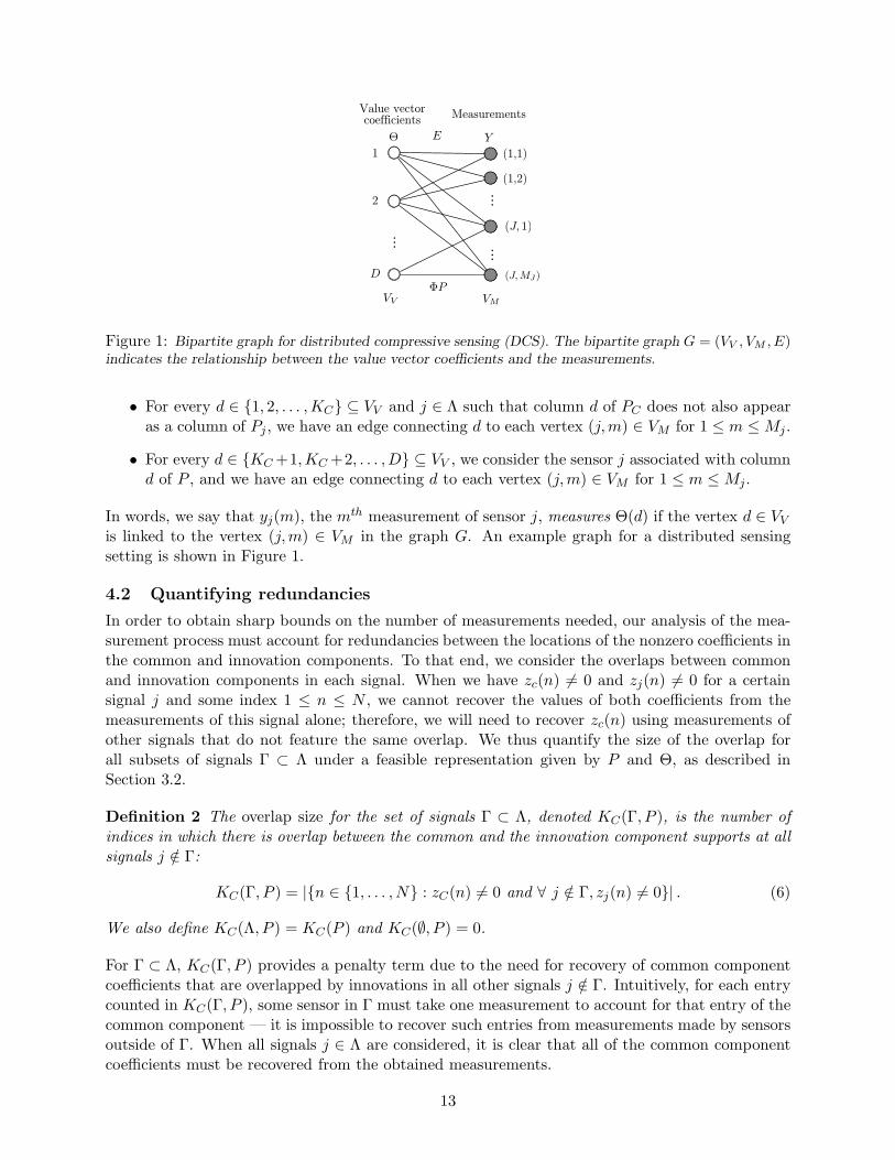
4.1 Modeling dependencies using bipartite graphs

We introduce a graphical representation that captures the dependencies between the measurementsin Y and the value vector Θ, represented by Φ and P . Consider a feasible decomposition of Xinto a full-rank matrix P ∈ PF (X) and the corresponding Θ; the matrix P defines the sparsitiesof the common and innovation components KC and Kj , 1 ≤ j ≤ J , as well as the joint sparsity

D = KC +∑J

j=1Kj . Define the following sets of vertices: (i) the set of value vertices VV haselements with indices d ∈ 1, . . . ,D representing the entries of the value vector Θ(d), and (ii) theset of measurement vertices VM has elements with indices (j,m) representing the measurementsyj(m), with j ∈ Λ and m ∈ 1, . . . ,Mj. The cardinalities for these sets are |VV | = D and|VM | = M , respectively.

We now introduce a bipartite graph G = (VV , VM , E), that represents the relationships betweenthe entries of the value vector and the measurements (see [4] for details). The set of edges E isdefined as follows:

12

Value vectorcoefficients Measurements

1

2

D

(1,1)

(1,2)

(J,MJ)

VM

...

...

...

Figure 1: Bipartite graph for distributed compressive sensing (DCS). The bipartite graph G = (VV , VM , E)indicates the relationship between the value vector coefficients and the measurements.

• For every d ∈ 1, 2, . . . ,KC ⊆ VV and j ∈ Λ such that column d of PC does not also appearas a column of Pj , we have an edge connecting d to each vertex (j,m) ∈ VM for 1 ≤ m ≤Mj .

• For every d ∈ KC +1,KC +2, . . . ,D ⊆ VV , we consider the sensor j associated with columnd of P , and we have an edge connecting d to each vertex (j,m) ∈ VM for 1 ≤ m ≤Mj.

In words, we say that yj(m), the mth measurement of sensor j, measures Θ(d) if the vertex d ∈ VV

is linked to the vertex (j,m) ∈ VM in the graph G. An example graph for a distributed sensingsetting is shown in Figure 1.

4.2 Quantifying redundancies

In order to obtain sharp bounds on the number of measurements needed, our analysis of the mea-surement process must account for redundancies between the locations of the nonzero coefficients inthe common and innovation components. To that end, we consider the overlaps between commonand innovation components in each signal. When we have zc(n) 6= 0 and zj(n) 6= 0 for a certainsignal j and some index 1 ≤ n ≤ N , we cannot recover the values of both coefficients from themeasurements of this signal alone; therefore, we will need to recover zc(n) using measurements ofother signals that do not feature the same overlap. We thus quantify the size of the overlap forall subsets of signals Γ ⊂ Λ under a feasible representation given by P and Θ, as described inSection 3.2.

Definition 2 The overlap size for the set of signals Γ ⊂ Λ, denoted KC(Γ, P ), is the number ofindices in which there is overlap between the common and the innovation component supports at allsignals j /∈ Γ:

KC(Γ, P ) = |n ∈ 1, . . . , N : zC(n) 6= 0 and ∀ j /∈ Γ, zj(n) 6= 0| . (6)

We also define KC(Λ, P ) = KC(P ) and KC(∅, P ) = 0.

For Γ ⊂ Λ, KC(Γ, P ) provides a penalty term due to the need for recovery of common componentcoefficients that are overlapped by innovations in all other signals j /∈ Γ. Intuitively, for each entrycounted in KC(Γ, P ), some sensor in Γ must take one measurement to account for that entry of thecommon component — it is impossible to recover such entries from measurements made by sensorsoutside of Γ. When all signals j ∈ Λ are considered, it is clear that all of the common componentcoefficients must be recovered from the obtained measurements.

13

4.3 Measurement bounds

Converse and achievable bounds for the number of measurements necessary for DCS recovery aregiven below. Our bounds consider each subset of sensors Γ ⊆ Λ, since the cost of sensing thecommon component can be amortized across sensors: it may be possible to reduce the rate at onesensor j1 ∈ Γ (up to a point), as long as other sensors in Γ offset the rate reduction. We quantifythe reduction possible through the following definition.

Definition 3 The conditional sparsity of the set of signals Γ is the number of entries of the vectorΘ that must be recovered by measurements yj, j ∈ Γ:

Kcond(Γ, P ) =

∑

j∈Γ

Kj(P )

+KC(Γ, P ).

The joint sparsity gives the number of degrees of freedom for the signals in Λ, while the conditionalsparsity gives the number of degrees of freedom for signals in Γ when the signals in Λ \ Γ areavailable as side information. Note also that Definition 1 for joint sparsity can be extended to asubset of signals Γ by considering the number of entries of Θ that affect these signals:

Kjoint(Γ, P ) = D −Kcond(Λ− Γ, P ) =

∑

j∈Γ

Kj(P )

+KC(P )−KC(Λ \ Γ, P ).

Note that Kcond(Λ, P ) = Kjoint(Λ, P ) = D.

The bipartite graph introduced in Section 4.1 is the cornerstone of Theorems 3, 4, and 5, whichconsider whether a perfect matching can be found in the graph; see the proofs in Appendices B, D,and E, respectively, for detail.

Theorem 3 (Achievable, known P ) Assume that a signal ensemble X is obtained from a com-mon/innovation component JSM P. Let M = (M1,M2, . . . ,MJ) be a measurement tuple, letΦjj∈Λ be random matrices having Mj rows of i.i.d. Gaussian entries for each j ∈ Λ, and writeY = ΦX. Suppose there exists a full rank location matrix P ∈ PF (X) such that

∑

j∈Γ

Mj ≥ Kcond(Γ, P ) (7)

for all Γ ⊆ Λ. Then with probability one over Φjj∈Γ, there exists a unique solution Θ to the system

of equations Y = ΦP Θ; hence, the signal ensemble X can be uniquely recovered as X = P Θ.

Theorem 4 (Achievable, unknown P ) Assume that a signal ensemble X and measurement matri-ces Φjj∈Λ follow the assumptions of Theorem 3. Suppose there exists a full rank location matrixP ∗ ∈ PF (X) such that ∑

j∈Γ

Mj ≥ Kcond(Γ, P ∗) + |Γ| (8)

for all Γ ⊆ Λ. Then X can be uniquely recovered from Y with probability one over Φjj∈Γ.

Theorem 5 (Converse) Assume that a signal ensemble X and measurement matrices Φjj∈Λ

follow the assumptions of Theorem 3. Suppose there exists a full rank location matrix P ∈ PF (X)such that ∑

j∈Γ

Mj < Kcond(Γ, P ) (9)

14

for some Γ ⊆ Λ. Then there exists a solution Θ such that Y = ΦP Θ but X := P Θ 6= X.

The identification of a feasible location matrix P causes the one measurement per sensor gap thatprevents (8)–(9) from being a tight converse and achievable bound pair. We note in passing that thesignal recovery procedure used in Theorem 4 is akin to ℓ0-norm minimization on X; see Appendix Dfor details.

4.4 Discussion

The bounds in Theorems 3–5 are dependent on the dimensionality of the subspaces in which thesignals reside. The number of noiseless measurements required for ensemble recovery is determinedby the dimensionality dim(S) of the subspace S in the relevant signal model, because dimensionalityand sparsity play a volumetric role akin to the entropy H used to characterize rates in sourcecoding. Whereas in source coding each bit resolves between two options, and 2NH typical inputsare described using NH bits [12], in CS we have M = dim(S) + O(1). Similar to Slepian-Wolfcoding [13], the number of measurements required for each sensor must account for the minimalfeatures unique to that sensor, while at the same time features that appear among multiple sensorsmust be amortized over the group.

Theorems 3–5 can also be applied to the single sensor and joint measurement settings. In thesingle-signal setting (Theorem 1), we will have x = Pθ with θ ∈ R

K , and Λ = 1; Theorem 4provides the requirement M ≥ K + 1. It is easy to show that the joint measurement is equivalentto the single-signal setting: we stack all the individual signals into a single signal vector, and inboth cases all measurements are dependent on all the entries of the signal vector. However, thedistribution of the measurements among the available sensors is irrelevant in a joint measurementsetting. Therefore, we only obtain a necessary condition

∑j Mj ≥ D + 1 on the total number of

measurements required.

5 Practical Recovery Algorithms and Experiments

Although we have provided a unifying theoretical treatment for the three JSM models, the nuanceswarrant further study. In particular, while Theorem 4 highlights the basic tradeoffs that mustbe made in partitioning the measurement budget among sensors, the result does not by designprovide insight into tractable algorithms for signal recovery. We believe there is additional insightto be gained by considering each model in turn, and while the presentation may be less unified, weattribute this to the fundamental diversity of problems that can arise under the umbrella of jointlysparse signal representations. In this section, we focus on tractable recovery algorithms for eachmodel and, when possible, analyze the corresponding measurement requirements.

5.1 Recovery strategies for sparse common + innovations (JSM-1)

We first characterize the sparse common signal and innovations model JSM-1 from Section 3.3.1.For simplicity, we limit our description to J = 2 signals, but describe extensions to multiple signalsas needed.

5.1.1 Measurement bounds for joint recovery

Under the JSM-1 model, separate recovery of the signal xj via ℓ0-norm minimization would requireKjoint(j) + 1 = Kcond(j) + 1 = KC +Kj −KC(Λ \ j) + 1 measurements, where KC(Λ \ j)accounts for sparsity reduction due to overlap between zC and zj . We apply Theorem 4 to the JSM-1 model to obtain the corollary below. To address the possibility of sparsity reduction, we denote

15

by KR the number of indices in which the common component zC and all innovation componentszj , j ∈ Λ overlap; this results in sparsity reduction for the common component.

Corollary 1 Assume the measurement matrices Φjj∈Λ contain i.i.d. Gaussian entries. Thenthe signal ensemble X can be recovered with probability one if the following conditions hold:

∑

j∈Γ

Mj ≥

∑

j∈Γ

Kj

+KC(Γ) + |Γ|, Γ 6= Λ,

∑

j∈Λ

Mj ≥ KC +

∑

j∈Λ

Kj

+ J −KR.

Our joint recovery scheme provides a significant savings in measurements, because the commoncomponent can be measured as part of any of the J signals.

5.1.2 Stochastic signal model for JSM-1

To give ourselves a firm footing for analysis, in the remainder of Section 5.1 we use a stochasticprocess for JSM-1 signal generation. This framework provides an information theoretic settingwhere we can scale the size of the problem and investigate which measurement rates enable recovery.We generate the common and innovation components as follows. For n ∈ 1, . . . , N the decisionwhether zC(n) and zj(n) is zero or not is an i.i.d. Bernoulli process, where the probability of anonzero value is given by parameters denoted SC and Sj , respectively. The values of the nonzerocoefficients are then generated from an i.i.d. Gaussian distribution. The outcome of this process isthat zC and zj have sparsities KC ∼ Binomial(N,SC) and Kj ∼ Binomial(N,Sj). The parametersSj and SC are sparsity rates controlling the random generation of each signal. Our model resemblesthe Gaussian spike process [58], which is a limiting case of a Gaussian mixture model.

Likelihood of sparsity reduction and overlap: This stochastic model can yield signalensembles for which the corresponding generating matrices P allow for sparsity reduction; specif-ically, there might be overlap between the supports of the common component zC and all theinnovation components zj , j ∈ Λ. For J = 2, the probability that a given index is present inall supports is SR := SCS1S2. Therefore, the distribution of the cardinality of this overlap isKR ∼ Binomial(N,SR). We must account for the reduction obtained from the removal of thecorresponding number of columns from the location matrix P when the total number of mea-surements M1 + M2 is considered. In the same way we can show that the distributions for thenumber of indices in the overlaps required by Corollary 1 are KC(1) ∼ Binomial(N,SC,1) andKC(2) ∼ Binomial(N,SC,2), where SC,1 := SC(1− S1)S2 and SC,2 := SCS1(1− S2).

Measurement rate region: To characterize DCS recovery performance, we introduce ameasurement rate region. We define the measurement rate Rj in an asymptotic manner as

Rj := limN→∞

Mj

N, j ∈ Λ.

Additionally, we note that

limN→∞

KC

N= SC and lim

N→∞

Kj

N= Sj, j ∈ Λ

Thus, we also set SXj= SC + Sj − SCSj, j ∈ 1, 2. For a measurement rate pair (R1, R2) and

sources X1 and X2, we evaluate whether we can recover the signals with vanishing probability oferror as N increases. In this case, we say that the measurement rate pair is achievable.

16

For jointly sparse signals under JSM-1, separate recovery via ℓ0-norm minimization wouldrequire a measurement rate Rj = SXj

. Separate recovery via ℓ1-norm minimization would requirean overmeasuring factor c(SXj

), and thus the measurement rate would becomeRj = SXj·c(SXj

). Toimprove upon these figures, we adapt the standard machinery of CS to the joint recovery problem.

5.1.3 Joint recovery via ℓ1-norm minimization

As discussed in Section 2.3, solving an ℓ0-norm minimization is NP-hard, and so in practice wemust relax our ℓ0 criterion in order to make the solution tractable. We now study what penaltymust be paid for ℓ1-norm recovery of jointly sparse signals. Using the vector and frame

Z :=

zCz1z2

and Φ :=

[Φ1 Φ1 0Φ2 0 Φ2

], (11)

we can represent the concatenated measurement vector Y sparsely using the concatenated coefficientvector Z, which contains KC+K1+K2−KR nonzero coefficients, to obtain Y = ΦZ. With sufficientovermeasuring, we have seen experimentally that it is possible to recover a vector Z, which yieldsxj = zC + zj , j = 1, 2, by solving the weighted ℓ1-norm minimization

Z = arg min γC ||zC ||1 + γ1||z1||1 + γ2||z2||1 s.t. y = ΦZ, (12)

where γC , γ1, γ2 ≥ 0. We call this the γ-weighted ℓ1-norm formulation; our numerical results(Section 5.1.6 and our technical report [59]) indicate a reduction in the requisite number of mea-surements via this enhancement. If K1 = K2 and M1 = M2, then without loss of generality we setγ1 = γ2 = 1 and numerically search for the best parameter γC . We discuss the asymmetric casewith K1 = K2 and M1 6= M2 in the technical report [59].

5.1.4 Converse bound on performance of γ-weighted ℓ1-norm minimization

We now provide a converse bound that describes what measurement rate pairs cannot be achievedvia the γ-weighted ℓ1-norm minimization. Our notion of a converse focuses on the setting whereeach signal xj is measured via multiplication by the Mj by N matrix Φj and joint recovery isperformed via our γ-weighted ℓ1-norm formulation (12). Within this setting, a converse region is aset of measurement rates for which the recovery fails with overwhelming probability as N increases.

We assume that J = 2 sources have innovation sparsity rates that satisfy S1 = S2 = SI .Our first result, proved in Appendix F, provides deterministic necessary conditions to recover thecomponents zC , z1, and z2, using the γ-weighted ℓ1-norm formulation (12). We note that the lemmaholds for all such combinations of components that generate the same signals x1 = zC + z1 andx2 = zC + z2.

Lemma 1 Consider any γC , γ1, and γ2 in the γ-weighted ℓ1-norm formulation (12). The com-ponents zC , z1, and z2 can be recovered using measurement matrices Φ1 and Φ2 only if (i) z1 canbe recovered via ℓ1-norm minimization (3) using Φ1 and measurements Φ1z1; (ii) z2 can be recov-ered via ℓ1-norm minimization using Φ2 and measurements Φ2z2; and (iii) zC can be recovered viaℓ1-norm minimization using the joint matrix [ΦT

1 ΦT2 ]T and measurements [ΦT

1 ΦT2 ]T zC .

Lemma 1 can be interpreted as follows. If M1 and M2 are not large enough individually, thenthe innovation components z1 and z2 cannot be recovered. This implies a converse bound on theindividual measurement rates R1 and R2. Similarly, combining Lemma 1 with the converse bound

17

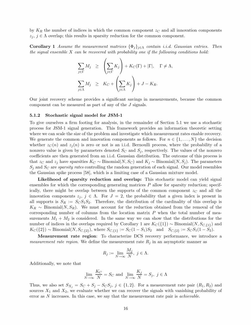
0 0.2 0.4 0.6 0.8 10

0.1

0.2

0.3

0.4

0.5

0.6

0.7

0.8

0.9

1

Simulation

R1

R2 Anticipated Converse

Achievable

Separate Recovery

Figure 2: Recovering a signal ensemble with sparse common + innovations (JSM-1). We chose acommon component sparsity rate SC = 0.2 and innovation sparsity rates SI = S1 = S2 = 0.05. Oursimulation results use the γ-weighted ℓ1-norm formulation (12) on signals of length N = 1000; themeasurement rate pairs that achieved perfect recovery over 100 simulations are denoted by circles.

of Theorem 2 for single-source ℓ1-norm minimization of the common component zC implies a lowerbound on the sum measurement rate R1 +R2.

Anticipated converse: As shown in Corollary 1, for indices n such that x1(n) and x2(n) differand are nonzero, each sensor must take measurements to account for one of the two coefficients. Inthe case where S1 = S2 = SI , the joint sparsity rate is SC +2SI−SCS

2I . We define the measurement

function c′(S) := S · c(S) based on Donoho and Tanner’s oversampling factor c(S) (Theorem 2).It can be shown that the function c′(·) is concave; in order to minimize the sum rate bound, we“explain” as many of the sparse coefficients in one of the signals and as few as possible in the other.From Corollary 1, we have R1, R2 ≥ SI + SCSI − SCS

2I . Consequently, one of the signals must

“explain” this sparsity rate, whereas the other signal must explain the rest:

[SC + 2SI − SCS2I ]− [SI + SCSI − SCS

2I ] = SC + SI − SCSI .

Unfortunately, the derivation of c′(S) relies on Gaussianity of the measurement matrix, whereasin our case Φ has a block matrix form. Therefore, the following conjecture remains to be provedrigorously.

Conjecture 1 Let J = 2 and fix the sparsity rate of the common component SC and the innovationsparsity rates S1 = S2 = SI . Then the following conditions on the measurement rates are necessaryto enable recovery with probability one:

Rj ≥ c′(SI + SCSI − SCS

2I

), j = 1, 2,

R1 +R2 ≥ c′(SI + SCSI − SCS

2I

)+ c′ (SC + SI − SCSI) .

5.1.5 Achievable bound on performance of ℓ1-norm minimization

We have not yet characterized the performance of γ-weighted ℓ1-norm formulation (12) analytically.Instead, Theorem 6 below uses an alternative ℓ1-norm based recovery technique. The proof describesa constructive recovery algorithm. We construct measurement matrices Φ1 and Φ2, each consisting

18

of two parts. The first parts of the matrices are identical and recover x1 − x2. The second parts ofthe matrices are different and enable the recovery of 1

2x1 + 12x2. Once these two components have

been recovered, the computation of x1 and x2 is straightforward. The measurement rate can becomputed by considering both identical and different parts of the measurement matrices.

Theorem 6 Let J = 2, N → ∞ and fix the sparsity rate of the common component SC and theinnovation sparsity rates S1 = S2 = SI . If the measurement rates satisfy the following conditions:

Rj > c′(2SI − S2I ), j = 1, 2, (13a)

R1 +R2 > c′(2SI − S2I ) + c′(SC + 2SI − 2SCSI − S

2I + SCS

2I ), (13b)

then we can design measurement matrices Φ1 and Φ2 with random Gaussian entries and an ℓ1-normminimization recovery algorithm that succeeds with probability approaching one as N increases.Furthermore, as SI → 0 the sum measurement rate approaches c′(SC).

The theorem is proved in Appendix G. The recovery algorithm of Theorem 6 is based on linearprogramming. It can be extended from J = 2 to an arbitrary number of signals by recovering allsignal differences of the form xj1−xj2 in the first stage of the algorithm and then recovering 1

J

∑j xj

in the second stage. In contrast, our γ-weighted ℓ1-norm formulation (12) recovers a length-JNsignal. Our simulation experiments (Section 5.1.6) indicate that the γ-weighted formulation canrecover using fewer measurements than the approach of Theorem 6.

The achievable measurement rate region of Theorem 6 is loose with respect to the region of theanticipated converse Conjecture 1 (see Figure 2). We leave for future work the characterization of atight measurement rate region for computationally tractable (polynomial time) recovery techniques.

5.1.6 Simulations for JSM-1

We now present simulation results for several different JSM-1 settings. The γ-weighted ℓ1-normformulation (12) was used throughout, where the optimal choice of γC , γ1, and γ2 depends on therelative sparsities KC , K1, and K2. The optimal values have not been determined analytically. In-stead, we rely on a numerical optimization, which is computationally intense. A detailed discussionof our intuition behind the choice of γ appears in the technical report [59].

Recovering two signals with symmetric measurement rates: Our simulation setting isas follows. The signal components zC , z1, and z2 are assumed (without loss of generality) to besparse in Ψ = IN with sparsities KC , K1, and K2, respectively. We assign random Gaussian valuesto the nonzero coefficients. We restrict our attention to the symmetric setting in which K1 = K2

and M1 = M2, and consider signals of length N = 50 where KC +K1 +K2 = 15.

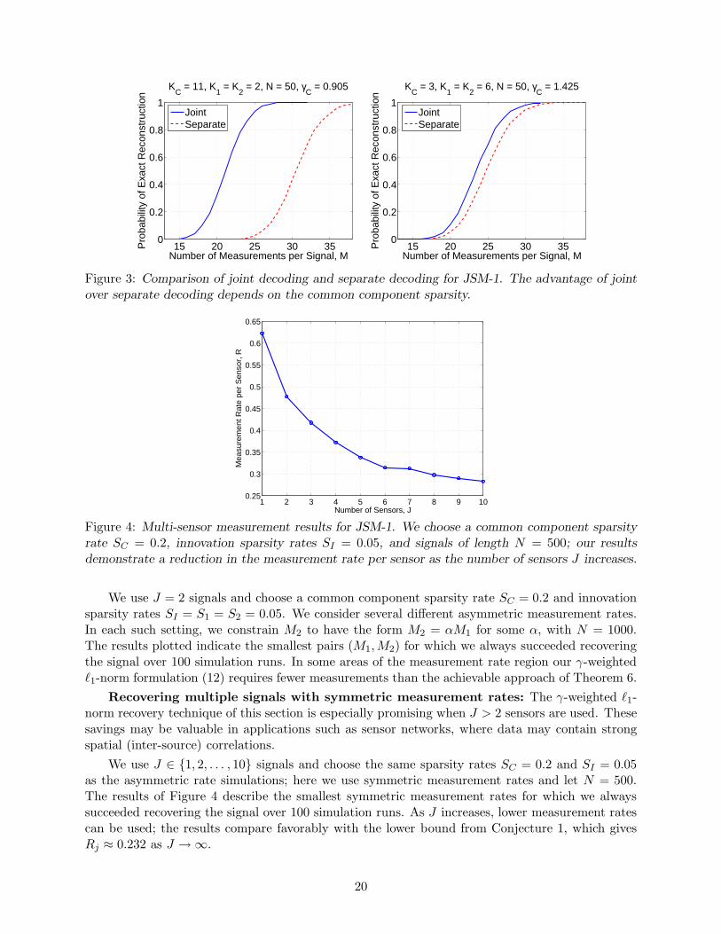
In our joint decoding simulations, we consider values of M1 and M2 in the range between 10and 40. We find the optimal γC in the γ-weighted ℓ1-norm formulation (12) using a line searchoptimization, where simulation indicates the “goodness” of specific γC values in terms of the like-lihood of recovery. With the optimal γC , for each set of values we run several thousand trials todetermine the empirical probability of success in decoding z1 and z2. The results of the simulationare summarized in Figure 3. The savings in the number of measurements M can be substantial,especially when the common component KC is large (Figure 3). For KC = 11, K1 = K2 = 2,M is reduced by approximately 30%. For smaller KC , joint decoding barely outperforms separatedecoding, since most of the measurements are expended on innovation components. Additionalresults appear in [59].

Recovering two signals with asymmetric measurement rates: In Figure 2, we compareseparate CS recovery with the anticipated converse bound of Conjecture 1, the achievable boundof Theorem 6, and numerical results.

19

15 20 25 30 350

0.2

0.4

0.6

0.8

1

Number of Measurements per Signal, M

Pro

babi

lity

of E

xact

Rec

onst

ruct

ion

KC

= 11, K1 = K

2 = 2, N = 50, γ

C = 0.905

JointSeparate

15 20 25 30 350

0.2

0.4

0.6

0.8

1

Number of Measurements per Signal, M

Pro

babi

lity

of E

xact

Rec

onst

ruct

ion

KC

= 3, K1 = K

2 = 6, N = 50, γ

C = 1.425

JointSeparate

Figure 3: Comparison of joint decoding and separate decoding for JSM-1. The advantage of jointover separate decoding depends on the common component sparsity.

1 2 3 4 5 6 7 8 9 100.25

0.3

0.35

0.4

0.45

0.5

0.55

0.6

0.65

Number of Sensors, J

Mea

sure

men

t Rat

e pe

r S

enso

r, R

Figure 4: Multi-sensor measurement results for JSM-1. We choose a common component sparsityrate SC = 0.2, innovation sparsity rates SI = 0.05, and signals of length N = 500; our resultsdemonstrate a reduction in the measurement rate per sensor as the number of sensors J increases.

We use J = 2 signals and choose a common component sparsity rate SC = 0.2 and innovationsparsity rates SI = S1 = S2 = 0.05. We consider several different asymmetric measurement rates.In each such setting, we constrain M2 to have the form M2 = αM1 for some α, with N = 1000.The results plotted indicate the smallest pairs (M1,M2) for which we always succeeded recoveringthe signal over 100 simulation runs. In some areas of the measurement rate region our γ-weightedℓ1-norm formulation (12) requires fewer measurements than the achievable approach of Theorem 6.

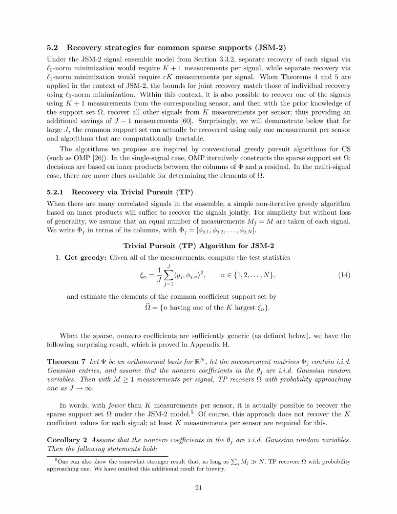
Recovering multiple signals with symmetric measurement rates: The γ-weighted ℓ1-norm recovery technique of this section is especially promising when J > 2 sensors are used. Thesesavings may be valuable in applications such as sensor networks, where data may contain strongspatial (inter-source) correlations.

We use J ∈ 1, 2, . . . , 10 signals and choose the same sparsity rates SC = 0.2 and SI = 0.05as the asymmetric rate simulations; here we use symmetric measurement rates and let N = 500.The results of Figure 4 describe the smallest symmetric measurement rates for which we alwayssucceeded recovering the signal over 100 simulation runs. As J increases, lower measurement ratescan be used; the results compare favorably with the lower bound from Conjecture 1, which givesRj ≈ 0.232 as J →∞.

20

5.2 Recovery strategies for common sparse supports (JSM-2)

Under the JSM-2 signal ensemble model from Section 3.3.2, separate recovery of each signal viaℓ0-norm minimization would require K + 1 measurements per signal, while separate recovery viaℓ1-norm minimization would require cK measurements per signal. When Theorems 4 and 5 areapplied in the context of JSM-2, the bounds for joint recovery match those of individual recoveryusing ℓ0-norm minimization. Within this context, it is also possible to recover one of the signalsusing K + 1 measurements from the corresponding sensor, and then with the prior knowledge ofthe support set Ω, recover all other signals from K measurements per sensor; thus providing anadditional savings of J − 1 measurements [60]. Surprisingly, we will demonstrate below that forlarge J , the common support set can actually be recovered using only one measurement per sensorand algorithms that are computationally tractable.

The algorithms we propose are inspired by conventional greedy pursuit algorithms for CS(such as OMP [26]). In the single-signal case, OMP iteratively constructs the sparse support set Ω;decisions are based on inner products between the columns of Φ and a residual. In the multi-signalcase, there are more clues available for determining the elements of Ω.

5.2.1 Recovery via Trivial Pursuit (TP)

When there are many correlated signals in the ensemble, a simple non-iterative greedy algorithmbased on inner products will suffice to recover the signals jointly. For simplicity but without lossof generality, we assume that an equal number of measurements Mj = M are taken of each signal.We write Φj in terms of its columns, with Φj = [φj,1, φj,2, . . . , φj,N ].

Trivial Pursuit (TP) Algorithm for JSM-2

1. Get greedy: Given all of the measurements, compute the test statistics

ξn =1

J

J∑

j=1

〈yj, φj,n〉2, n ∈ 1, 2, . . . , N, (14)

and estimate the elements of the common coefficient support set by

Ω = n having one of the K largest ξn.

When the sparse, nonzero coefficients are sufficiently generic (as defined below), we have thefollowing surprising result, which is proved in Appendix H.

Theorem 7 Let Ψ be an orthonormal basis for RN , let the measurement matrices Φj contain i.i.d.

Gaussian entries, and assume that the nonzero coefficients in the θj are i.i.d. Gaussian randomvariables. Then with M ≥ 1 measurements per signal, TP recovers Ω with probability approachingone as J →∞.

In words, with fewer than K measurements per sensor, it is actually possible to recover thesparse support set Ω under the JSM-2 model.5 Of course, this approach does not recover the Kcoefficient values for each signal; at least K measurements per sensor are required for this.

Corollary 2 Assume that the nonzero coefficients in the θj are i.i.d. Gaussian random variables.Then the following statements hold:

5One can also show the somewhat stronger result that, as long asP

jMj ≫ N , TP recovers Ω with probability

approaching one. We have omitted this additional result for brevity.

21

1. Let the measurement matrices Φj contain i.i.d. Gaussian entries, with each matrix having anovermeasuring factor of c = 1 (that is, Mj = K for each measurement matrix Φj). Then TPrecovers all signals from the ensemble xj with probability approaching one as J →∞.

2. Let Φj be a measurement matrix with overmeasuring factor c < 1 (that is, Mj < K), forsome j ∈ Λ. Then with probability one, the signal xj cannot be uniquely recovered by anyalgorithm for any value of J .

The first statement is an immediate corollary of Theorem 7; the second statement followsbecause each equation yj = Φjxj would be underdetermined even if the nonzero indices wereknown. Thus, under the JSM-2 model, the TP algorithm asymptotically performs as well asan oracle decoder that has prior knowledge of the locations of the sparse coefficients. From aninformation theoretic perspective, Corollary 2 provides tight achievable and converse bounds forJSM-2 signals. We should note that the theorems in this section have a slightly different flavorthan Theorem 4 and 5, which ensure recovery of any sparse signal ensemble, given a suitable setof measurement matrices. Theorem 7 and Corollary 2 above, in contrast, rely on a random signalmodel and do not guarantee simultaneous performance for all sparse signals under any particularmeasurement ensemble. Nonetheless, we feel this result is worth presenting to highlight the strongsubspace concentration behavior that enables the correct identification of the common support.

In the technical reports [59, 61], we derive an approximate formula for the probability of errorin recovering the common support set Ω given J , K, M , and N . While theoretically interesting andpotentially practically useful, these results require J to be large. Our numerical experiments showthat the number of measurements required for recovery using TP decreases quickly as J increases.However, in the case of small J , TP performs poorly. Hence, we propose next an alternativerecovery technique based on simultaneous greedy pursuit that performs well for small J .

5.2.2 Recovery via iterative greedy pursuit

In practice, the common sparse support among the J signals enables a fast iterative algorithmto recover all of the signals jointly. Tropp and Gilbert have proposed one such algorithm, calledSimultaneous Orthogonal Matching Pursuit (SOMP) [53], which can be readily applied in our DCSframework. SOMP is a variant of OMP that seeks to identify Ω one element at a time. A similarsimultaneous sparse approximation algorithm has been proposed using convex optimization [62].We dub the DCS-tailored SOMP algorithm DCS-SOMP.

To adapt the original SOMP algorithm to our setting, we first extend it to cover a differentmeasurement matrix Φj for each signal xj. Then, in each DCS-SOMP iteration, we select thecolumn index n ∈ 1, 2, . . . , N that accounts for the greatest amount of residual energy acrossall signals. As in SOMP, we orthogonalize the remaining columns (in each measurement matrix)after each step; after convergence we obtain an expansion of the measurement vector yj on anorthogonalized subset of the columns of basis vectors. To obtain the expansion coefficients in thesparse basis, we then reverse the orthogonalization process using the QR matrix factorization.Finally, we again assume that Mj = M measurements per signal are taken.

DCS-SOMP Algorithm for JSM-2

1. Initialize: Set the iteration counter ℓ = 1. For each signal index j ∈ Λ, initialize theorthogonalized coefficient vectors βj = 0, βj ∈ R

M ; also initialize the set of selected indices

Ω = ∅. Let rj,ℓ denote the residual of the measurement yj remaining after the first ℓ iterations,and initialize rj,0 = yj .

22

2. Select the dictionary vector that maximizes the value of the sum of the magnitudes of theprojections of the residual, and add its index to the set of selected indices

nℓ = arg maxn∈1,...,N

J∑

j=1

|〈rj,ℓ−1, φj,n〉|

‖φj,n‖2,

Ω = [Ω nℓ].

3. Orthogonalize the selected basis vector against the orthogonalized set of previously selecteddictionary vectors

γj,ℓ = φj,nℓ−

ℓ−1∑

t=0

〈φj,nℓ, γj,t〉

‖γj,t‖22γj,t.

4. Iterate: Update the estimate of the coefficients for the selected vector and residuals

βj(ℓ) =〈rj,ℓ−1, γj,ℓ〉

‖γj,ℓ‖22

,

rj,ℓ = rj,ℓ−1 −〈rj,ℓ−1, γj,ℓ〉

‖γj,ℓ‖22γj,ℓ.

5. Check for convergence: If ‖rj,ℓ‖2 > ǫ‖yj‖2 for all j, then increment ℓ and go to Step2; otherwise, continue to Step 6. The parameter ǫ determines the target error power levelallowed for algorithm convergence.

6. De-orthogonalize: Consider the relationship between Γj = [γj,1, γj,2, . . . , γj,M ] and the Φj

given by the QR factorization Φj,bΩ

= ΓjRj , where Φj,bΩ

= [φj,n1, φj,n2, . . . , φj,nM] is the so-

called mutilated basis.6 Since yj = Γjβj = Φj,bΩxj,bΩ = ΓjRjxj,bΩ, where xj,bΩ is the mutilated

coefficient vector, we can compute the signal estimates xj as

xj,bΩ = R−1j βj ,

where xj,bΩ

is the mutilated version of the sparse coefficient vector xj.

In practice, we obtain cK measurements from each signal xj for some value of c. We then useDCS-SOMP to recover the J signals jointly. We orthogonalize because as the number of iterationsapproaches M the norms of the residues of an orthogonal pursuit decrease faster than for a non-orthogonal pursuit; indeed, due to Step 3 the algorithm can only run for up to M iterations. Thecomputational complexity of this algorithm is O(JNM2), which matches that of separate recoveryfor each signal while reducing the required number of measurements.

Thanks to the common sparsity structure among the signals, we believe (but have not proved)that DCS-SOMP will succeed with c < c(S). Empirically, we have observed that a small numberof measurements proportional to K suffices for a moderate number of sensors J . Based on ourobservations, described in Section 5.2.3, we conjecture that K + 1 measurements per sensor sufficeas J → ∞. Thus, this efficient greedy algorithm enables an overmeasuring factor c = (K + 1)/Kthat approaches 1 as J , K, and N increase.

6We define a mutilated basis ΦΩ as a subset of the basis vectors from Φ = [φ1, φ2, . . . , φN ] corresponding to theindices given by the set Ω = n1, n2, . . . , nM, that is, ΦΩ = [φn1

, φn2, . . . , φnM

]. This concept can be extended tovectors in the same manner.

23

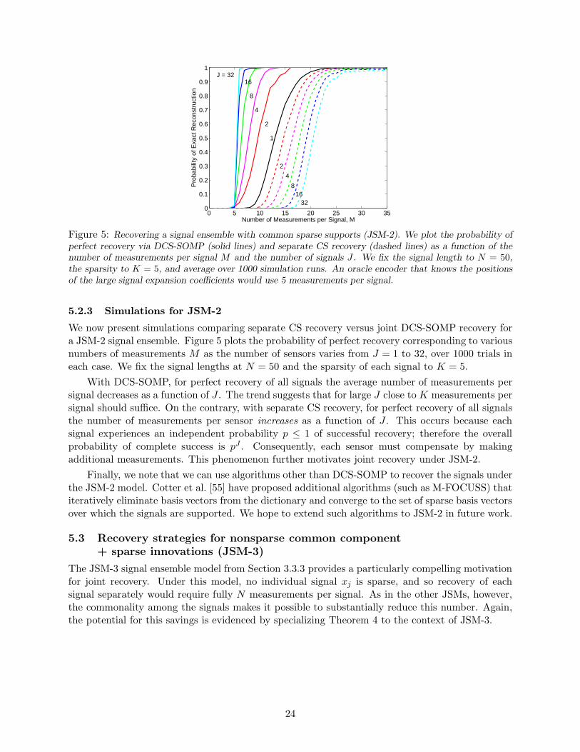
0 5 10 15 20 25 30 350

0.1

0.2

0.3

0.4

0.5

0.6

0.7

0.8

0.9

1

Number of Measurements per Signal, M

Pro

babi

lity

of E

xact

Rec

onst

ruct

ion

1

2

2

4

4

8

8

16

16

J = 32

32

Figure 5: Recovering a signal ensemble with common sparse supports (JSM-2). We plot the probability ofperfect recovery via DCS-SOMP (solid lines) and separate CS recovery (dashed lines) as a function of thenumber of measurements per signal M and the number of signals J . We fix the signal length to N = 50,the sparsity to K = 5, and average over 1000 simulation runs. An oracle encoder that knows the positionsof the large signal expansion coefficients would use 5 measurements per signal.

5.2.3 Simulations for JSM-2

We now present simulations comparing separate CS recovery versus joint DCS-SOMP recovery fora JSM-2 signal ensemble. Figure 5 plots the probability of perfect recovery corresponding to variousnumbers of measurements M as the number of sensors varies from J = 1 to 32, over 1000 trials ineach case. We fix the signal lengths at N = 50 and the sparsity of each signal to K = 5.

With DCS-SOMP, for perfect recovery of all signals the average number of measurements persignal decreases as a function of J . The trend suggests that for large J close to K measurements persignal should suffice. On the contrary, with separate CS recovery, for perfect recovery of all signalsthe number of measurements per sensor increases as a function of J . This occurs because eachsignal experiences an independent probability p ≤ 1 of successful recovery; therefore the overallprobability of complete success is pJ . Consequently, each sensor must compensate by makingadditional measurements. This phenomenon further motivates joint recovery under JSM-2.

Finally, we note that we can use algorithms other than DCS-SOMP to recover the signals underthe JSM-2 model. Cotter et al. [55] have proposed additional algorithms (such as M-FOCUSS) thatiteratively eliminate basis vectors from the dictionary and converge to the set of sparse basis vectorsover which the signals are supported. We hope to extend such algorithms to JSM-2 in future work.

5.3 Recovery strategies for nonsparse common component+ sparse innovations (JSM-3)

The JSM-3 signal ensemble model from Section 3.3.3 provides a particularly compelling motivationfor joint recovery. Under this model, no individual signal xj is sparse, and so recovery of eachsignal separately would require fully N measurements per signal. As in the other JSMs, however,the commonality among the signals makes it possible to substantially reduce this number. Again,the potential for this savings is evidenced by specializing Theorem 4 to the context of JSM-3.

24

Corollary 3 If Φj is a random Gaussian matrix for all j ∈ Λ, P is defined by JSM-3, and

∑

j∈Γ

Mj ≥∑

j∈Γ

Kj +KC(Γ, P ) + |Γ|, Γ ∈ Λ, (15)

∑

j∈Λ

Mj ≥∑

j∈Λ

Kj +N + J −KR, (16)

then the signal ensemble X can be uniquely recovered from Y with probability one.

This suggests that the number of measurements of an individual signal can be substantiallydecreased, as long as the total number of measurements is sufficiently large to capture enoughinformation about the nonsparse common component zC . The term KR denotes the number ofindices where the common and all innovation components overlap, and appears due to the sparsityreduction that can be performed at the common component before recovery. We also note thatwhen the supports of the innovations are independent, as J →∞, it becomes increasingly unlikelythat a given index will be included in all innovations, and thus the terms KC(Γ, P ) and KR will goto zero. On the other hand, when the supports are completely matched (implying Kj = K, j ∈ Λ),we will have KR = K, and after sparsity reduction has been addressed, KC(Γ, P ) = 0 for all Γ ⊆ Λ.

5.3.1 Recovery via Transpose Estimation of Common Component (TECC)

Successful recovery of the signal ensemble xj requires recovery of both the nonsparse commoncomponent zC and the sparse innovations zj. To help build intuition about how we mightaccomplish signal recovery using far fewer than N measurements per sensor, consider the followingthought experiment.

If zC were known, then each innovation zj could be estimated using the standard single-signalCS machinery on the adjusted measurements yj−ΦjzC = Φjzj . While zC is not known in advance,it can be estimated from the measurements. In fact, across all J sensors, a total of

∑j∈ΛMj random

projections of zC are observed (each corrupted by a contribution from one of the zj). Since zC isnot sparse, it cannot be recovered via CS techniques, but when the number of measurements issufficiently large (

∑j∈ΛMj ≫ N), zC can be estimated using standard tools from linear algebra.

A key requirement for such a method to succeed in recovering zC is that each Φj be different, sothat their rows combine to span all of R

N . In the limit (again, assuming the sparse innovationcoefficients are well-behaved), the common component zC can be recovered while still allowing eachsensor to operate at the minimum measurement rate dictated by the zj. A prototype algorithmis listed below, where we assume that each measurement matrix Φj has i.i.d. N (0, σ2

j ) entries.

TECC Algorithm for JSM-3

1. Estimate common component: Define the matrix Φ as the vertical concatenation of theregularized individual measurement matrices Φj = 1

Mjσ2j

Φj, that is, Φ = [ΦT1 , Φ

T2 , . . . , Φ

TJ ]T .

Calculate the estimate of the common component as zC = 1J ΦTY .

2. Estimate measurements generated by innovations: Using the previous estimate, sub-tract the contribution of the common part from the measurements and generate estimates forthe measurements caused by the innovations for each signal: yj = yj − Φj zC .

3. Recover innovations: Using a standard single-signal CS recovery algorithm,7 obtain esti-mates of the innovations zj from the estimated innovation measurements yj.

7For tractable analysis of the TECC algorithm, the proof of Theorem 8 employs a least-squares variant of ℓ0-normminimization.

25

4. Obtain signal estimates: Estimate each signal as the sum of the common and innovationsestimates; that is, xj = zC + zj .

The following theorem, proved in Appendix I, shows that asymptotically, by using the TECCalgorithm, each sensor needs to only measure at the rate dictated by the sparsity Kj .

Theorem 8 Assume that the nonzero expansion coefficients of the sparse innovations zj are i.i.d.Gaussian random variables and that their locations are uniformly distributed on 1, 2, . . . , N. Letthe measurement matrices Φj contain i.i.d. N (0, σ2

j ) entries with Mj ≥ Kj + 1. Then each signalxj can be recovered using the TECC algorithm with probability approaching one as J →∞.

For large J , the measurement rates permitted by Theorem 8 are the best possible for anyrecovery strategy for JSM-3 signals, even neglecting the presence of the nonsparse component.These rates meet the minimum bounds suggested by Corollary 3, although again Theorem 8 is ofa slightly different flavor, as it does not provide a uniform guarantee for all sparse signal ensemblesunder any particular measurement matrix collection. The CS technique employed in Theorem 8involves combinatorial searches that estimate the innovation components; we have provided thetheorem simply as support for our intuitive development of the TECC algorithm. More efficienttechniques could also be employed (including several proposed for CS in the presence of noise [25, 63,64]). It is reasonable to expect similar behavior; as the error in estimating the common componentdiminishes, these techniques should perform similarly to their noiseless analogues.

5.3.2 Recovery via Alternating Common and Innovation Estimation (ACIE)

The preceding analysis demonstrates that the number of required measurements in JSM-3 can besubstantially reduced through joint recovery. While Theorem 8 shows theoretical gains as J →∞,practical gains can also be realized with a moderate number of sensors. In particular, supposein the TECC algorithm that the initial estimate zC is not accurate enough to enable correctidentification of the sparse innovation supports Ωj. In such a case, it may still be possible fora rough approximation of the innovations zj to help refine the estimate zC . This in turn couldhelp to refine the estimates of the innovations.

The Alternating Common and Innovation Estimation (ACIE) algorithm exploits the observa-tion that once the basis vectors comprising the innovation zj have been identified in the index setΩj, their effect on the measurements yj can be removed to aid in estimating zC . Suppose that we

have an estimate for these innovation basis vectors in Ωj. We can then partition the measurementsinto two parts: the projection into span(φj,nn∈bΩj

) and the component orthogonal to that span.

We build a basis for the RMj where yj lives:

Bj = [Φj,bΩjQj ],

where Φj,bΩjis the mutilated matrix Φj corresponding to the indices in Ωj, and the Mj×(Mj−|Ωj|)

matrix Qj has orthonormal columns that span the orthogonal complement of Φj,bΩj.

This construction allows us to remove the projection of the measurements into the aforemen-tioned span to obtain measurements caused exclusively by vectors not in Ωj:

yj = QTj yj and Φj = QT

j Φj. (17)

These modifications enable the sparse decomposition of the measurement, which now lives in

RMj−|bΩj |, to remain unchanged:

26

yj =

N∑

n=1

αjφj,n.

Thus, the modified measurements Y =[yT1 yT

2 . . . yTJ

]Tand modified measurement matrix Φ =[

ΦT1 ΦT

2 . . . ΦTJ

]Tcan be used to refine the estimate of the common component of the signal,

zC = Φ†Y , (18)

where A† = (ATA)−1AT denotes the pseudoinverse of matrix A.

When the innovation support estimate is correct (Ωj = Ωj), the measurements yj will describeonly the common component zC . If this is true for every signal j and the number of remainingmeasurements

∑Jj=1(Mj −Kj) ≥ N , then zC can be perfectly recovered via (18). However, it may

be difficult to obtain correct estimates for all signal supports in the first iteration of the algorithm,and so we find it preferable to refine the estimate of the support by executing several iterations.

ACIE Algorithm for JSM-3

1. Initialize: Set Ωj = ∅ for each j. Set the iteration counter ℓ = 1.

2. Estimate common component: Update estimate zC according to (17)–(18).

3. Estimate innovation supports: For each sensor j, after subtracting the contribution zCfrom the measurements, yj = yj − Φj zC , estimate the support of each signal innovation Ωj.

4. Iterate: If ℓ < L, a preset number of iterations, then increment ℓ and return to Step 2.Otherwise proceed to Step 5.

5. Estimate innovation coefficients: For each j, estimate the coefficients for the indices inΩj,

zj,bΩj= Φ†

j,bΩj

(yj − Φj zC),

where zj,bΩj

is a mutilated version of the innovation’s sparse coefficient vector estimate zj .

6. Recover signals: Compute the estimate of each signal as xj = zC + zj .

Estimation of the supports in Step 3 can be accomplished using a variety of techniques. Wepropose to run a fixed number of iterations of OMP; if the supports of the innovations are knownto match across signals — as in JSM-2 — then more powerful algorithms like SOMP can be used.The ACIE algorithm is similar in spirit to other iterative estimation algorithms, such as turbodecoding [65].

5.3.3 Simulations for JSM-3

We now present simulations of JSM-3 recovery for the following scenario. Consider J signals oflength N = 50 containing a common white noise component zC(n) ∼ N (0, 1) for n ∈ 1, . . . , N.Each innovations component zj has sparsity K = 5 (once again in the time domain), resulting inxj = zC + zj . The signals are generated according to the model used in Section 5.1.6.

We study two different cases. The first is an extension of JSM-1: we select the supports for thevarious innovations separately and then apply OMP to each signal in Step 3 of the ACIE algorithmin order to estimate its innovations component. The second case is an extension of JSM-2: we selectone common support for all of the innovations across the signals and then apply the DCS-SOMPalgorithm (Section 5.2.2) to estimate the innovations in Step 3. In both cases we use L = 10

27

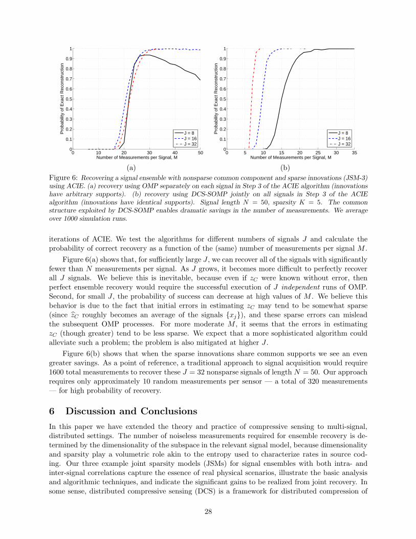
0 10 20 30 40 500

0.1

0.2

0.3

0.4

0.5

0.6

0.7

0.8

0.9

1

Number of Measurements per Signal, M

Pro

babi

lity

of E

xact

Rec

onst

ruct

ion

J = 8J = 16J = 32

0 5 10 15 20 25 30 350

0.1

0.2

0.3

0.4

0.5

0.6

0.7

0.8

0.9

1

Number of Measurements per Signal, M

Pro

babi

lity

of E

xact

Rec

onst

ruct

ion

J = 8J = 16J = 32

(a) (b)

Figure 6: Recovering a signal ensemble with nonsparse common component and sparse innovations (JSM-3)using ACIE. (a) recovery using OMP separately on each signal in Step 3 of the ACIE algorithm (innovationshave arbitrary supports). (b) recovery using DCS-SOMP jointly on all signals in Step 3 of the ACIEalgorithm (innovations have identical supports). Signal length N = 50, sparsity K = 5. The commonstructure exploited by DCS-SOMP enables dramatic savings in the number of measurements. We averageover 1000 simulation runs.

iterations of ACIE. We test the algorithms for different numbers of signals J and calculate theprobability of correct recovery as a function of the (same) number of measurements per signal M .

Figure 6(a) shows that, for sufficiently large J , we can recover all of the signals with significantlyfewer than N measurements per signal. As J grows, it becomes more difficult to perfectly recoverall J signals. We believe this is inevitable, because even if zC were known without error, thenperfect ensemble recovery would require the successful execution of J independent runs of OMP.Second, for small J , the probability of success can decrease at high values of M . We believe thisbehavior is due to the fact that initial errors in estimating zC may tend to be somewhat sparse(since zC roughly becomes an average of the signals xj), and these sparse errors can misleadthe subsequent OMP processes. For more moderate M , it seems that the errors in estimatingzC (though greater) tend to be less sparse. We expect that a more sophisticated algorithm couldalleviate such a problem; the problem is also mitigated at higher J .

Figure 6(b) shows that when the sparse innovations share common supports we see an evengreater savings. As a point of reference, a traditional approach to signal acquisition would require1600 total measurements to recover these J = 32 nonsparse signals of length N = 50. Our approachrequires only approximately 10 random measurements per sensor — a total of 320 measurements— for high probability of recovery.

6 Discussion and Conclusions

In this paper we have extended the theory and practice of compressive sensing to multi-signal,distributed settings. The number of noiseless measurements required for ensemble recovery is de-termined by the dimensionality of the subspace in the relevant signal model, because dimensionalityand sparsity play a volumetric role akin to the entropy used to characterize rates in source cod-ing. Our three example joint sparsity models (JSMs) for signal ensembles with both intra- andinter-signal correlations capture the essence of real physical scenarios, illustrate the basic analysisand algorithmic techniques, and indicate the significant gains to be realized from joint recovery. Insome sense, distributed compressive sensing (DCS) is a framework for distributed compression of

28

sources with memory, which has remained a challenging problem for some time.

In addition to offering substantially reduced measurement rates, the DCS-based distributedsource coding schemes we develop here share the properties of CS mentioned in Section 2. Twoadditional properties of DCS make it well-matched to distributed applications such as sensor net-works and arrays [51, 52]. First, each sensor encodes its measurements separately, which eliminatesthe need for inter-sensor communication. Second, DCS distributes its computational complexityasymmetrically, placing most of it in the joint decoder, which will often have more computationalresources than any individual sensor node. The encoders are very simple; they merely computeincoherent projections with their signals and make no decisions.

There are many opportunities for applications and extensions of these ideas. First, naturalsignals are not exactly sparse but rather can be better modeled as ℓp-compressible with 0 < p ≤1. Roughly speaking, a signal in a weak-ℓp ball has coefficients that decay as n−1/p once sortedaccording to magnitude [24]. The key concept is that the ordering of these coefficients is important.For JSM-2, we can extend the notion of simultaneous sparsity for ℓp-sparse signals whose sortedcoefficients obey roughly the same ordering [66]. This condition could perhaps be enforced as anℓp constraint on the composite signal

J∑

j=1

|xj(1)|,J∑

j=1

|xj(2)|, . . . ,J∑

j=1

|xj(N)|

.

Second, (random) measurements are real numbers; quantization gradually degrades the recov-ery quality as the quantization becomes coarser [34, 67, 68]. Moreover, in many practical situationssome amount of measurement noise will corrupt the xj, making them not exactly sparse in anybasis. While characterizing these effects and the resulting rate-distortion consequences in the DCSsetting are topics for future work, there has been work in the single-signal CS literature that weshould be able to leverage, including variants of Basis Pursuit with Denoising [63, 69], robust iter-ative recovery algorithms [64], CS noise sensitivity analysis [25, 34], the Dantzig Selector [33], andone-bit CS [70].

Third, in some applications, the linear program associated with some DCS decoders (in JSM-1and JSM-3) could prove too computationally intense. As we saw in JSM-2, efficient iterative andgreedy algorithms could come to the rescue, but these need to be extended to the multi-signalcase. Recent results on recovery from a union of subspaces give promise for efficient, model-basedalgorithms [66].

Finally, we focused our theory on models that assign common and innovation componentsto the signals in the ensemble. Other models tailored to specific applications can be posed; forexample, in hyperspectral imaging applications, it is common to obtain strong correlations onlyacross spectral slices within a certain neighborhood. It would be then appropriate to pose acommon/innovation model with separate common components that are localized to a subset of thespectral slices obtained. Results similar to those obtained in Section 4 are simple to derive formodels with full-rank location matrices.

A Proof of Theorem 1

Statement 2 is an application of the achievable bound of Theorem 4 to the case of J = 1 signal. Itremains then to prove Statements 1 and 3.

29

Statement 1 (Achievable, M ≥ 2K): We first note that, if K ≥ N/2, then with probabilityone, the matrix Φ has rank N , and there is a unique (correct) recovery. Thus we assume thatK < N/2. With probability one, all subsets of up to 2K columns drawn from Φ are linearlyindependent. Assuming this holds, then for two index sets Ω 6= Ω such that |Ω| = |Ω| = K,colspan(ΦΩ)∩colspan(ΦbΩ) has dimension equal to the number of indices common to both Ω and Ω.A signal projects to this common space only if its coefficients are nonzero on exactly these (fewerthan K) common indices; since ‖θ‖0 = K, this does not occur. Thus every K-sparse signal projectsto a unique point in R

M .

Statement 3 (Converse, M ≤ K): If M < K, there is insufficient information in the vectory to recover the K nonzero coefficients of θ; thus we assume M = K. In this case, there is asingle explanation for the measurements only if there is a single set Ω of K linearly independentcolumns and the nonzero indices of θ are the elements of Ω. Aside from this pathological case, therank of subsets ΦbΩ will generally be less than K — which would prevent robust recovery of signals

supported on Ω, or will be equal to K — which would give ambiguous solutions among all suchsets Ω.

B Proof of Theorem 3

We letD := KC +

∑

j∈Λ

Kj (19)

denote the number of columns in P . Because P ∈ PF (X), there exists Θ ∈ RD such that X = PΘ.

Because Y = ΦX, Θ is a solution to Y = ΦPΘ. We will argue that, with probability one over Φ,

Υ := ΦP

has rank D, and thus Θ is the unique solution to the equation Y = ΦPΘ = ΥΘ.

We recall that, under our common/innovation model, P has the form (5), where PC is anN × KC submatrix of the N × N identity, and each Pj , j ∈ Λ, is an N × Kj submatrix of theN ×N identity. To prove that Υ has rank D, we will require the following lemma, which we provein Appendix C.

Lemma 2 If (7) holds, then there exists a mapping C : 1, 2, . . . ,KC → Λ, assigning each elementof the common component to one of the sensors, such that for each Γ ⊆ Λ,

∑

j∈Γ

Mj ≥∑

j∈Γ

Kj +

KC∑

k=1

1C(k)∈Γ (20)

and such that for each k ∈ 1, 2, . . . ,KC, the kth column of PC is not a column of PC(k).

Intuitively, the existence of such a mapping suggests that (i) each sensor has taken enoughmeasurements to cover its own innovation (requiring Kj measurements) and perhaps some of thecommon component, (ii) for any Γ ⊆ Λ, the sensors in Γ have collectively taken enough extrameasurements to cover the requisite KC(Γ, P ) elements of the common component, and (iii) theextra measurements are taken at sensors where the common and innovation components do notoverlap. Formally, we will use the existence of such a mapping to prove that Υ has rank D.

30

We proceed by noting that Υ has the form

Υ =

Φ1PC Φ1P1 0 . . . 0Φ2PC 0 Φ2P2 . . . 0

......

.... . .

...ΦJPC 0 0 . . . ΦJPJ

,

where each ΦjPC (respectively, ΦjPj) is an Mj × KC (respectively, Mj × Kj) submatrix of Φj

obtained by selecting columns from Φj according to the nonzero entries of PC (respectively, Pj).In total, Υ has D columns (19). To argue that Υ has rank D, we will consider a sequence of threematrices Υ0, Υ1, and Υ2 constructed from small modifications to Υ.

We begin by letting Υ0 denote the “partially zeroed” matrix obtained from Υ using the followingconstruction. We first let Υ0 = Υ and then make the following adjustments:

1. Let k = 1.

2. For each j such that Pj has a column that matches column k of PC (note that by Lemma 2this cannot happen if C(k) = j), let k′ represent the column index of the full matrix P wherethis column of Pj occurs. Subtract column k′ of Υ0 from column k of Υ0. This forces to zeroall entries of Υ0 formerly corresponding to column k of the block ΦjPC .

3. If k < KC , add one to k and go to step 2.

The matrix Υ0 is identical to Υ everywhere except on the first KC columns, where any portion of acolumn overlapping with a column of ΦjPj to its right has been set to zero. Thus, Υ0 satisfies thenext two properties, which will be inherited by matrices Υ1 and Υ2 that we subsequently define:

P1. Each entry of Υ0 is either zero or a Gaussian random variable.

P2. All Gaussian random variables in Υ0 are i.i.d.

Finally, because Υ0 was constructed only by subtracting columns of Υ from one another,

rank(Υ0) = rank(Υ). (21)

We now let Υ1 be the matrix obtained from Υ0 using the following construction. For eachj ∈ Λ, we select Kj +

∑KC

k=1 1C(k)=j arbitrary rows from the portion of Υ0 corresponding to sensorj. Using (19), the resulting matrix Υ1 has

∑

j∈Λ

(Kj +

KC∑

k=1

1C(k)=j

)=∑

j∈Λ

Kj +KC = D

rows. Also, because Υ1 was obtained by selecting a subset of rows from Υ0, it has D columns andsatisfies

rank(Υ1) ≤ rank(Υ0). (22)

We now let Υ2 be the D×D matrix obtained by permuting columns of Υ1 using the followingconstruction:

1. Let Υ2 = [ ], and let j = 1.

31

2. For each k such that C(k) = j, let Υ1(k) denote the kth column of Υ1, and concatenate Υ1(k)to Υ2, i.e., let Υ2 ← [Υ2 Υ1(k)]. There are

∑KC

k=1 1C(k)=j such columns.

3. Let Υ′1 denote the columns of Υ1 corresponding to the entries of ΦjPj (the innovation com-

ponents of sensor j), and concatenate Υ′1 to Υ2, i.e., let Υ2 ← [Υ2 Υ′

1]. There are Kj suchcolumns.

4. If j < J , let j ← j + 1 and go to Step 2.

Because Υ1 and Υ2 share the same columns up to reordering, it follows that

rank(Υ2) = rank(Υ1). (23)

Based on its dependency on Υ0, and following from Lemma 2, the square matrix Υ2 meets propertiesP1 and P2 defined above in addition to a third property:

P3. All diagonal entries of Υ2 are Gaussian random variables.

This follows because for each j, Kj +∑KC

k=1 1C(k)=j rows of Υ1 are assigned in its construction, while

Kj +∑KC

k=1 1C(k)=j columns of Υ2 are assigned in its construction. Thus, each diagonal element ofΥ2 will either be an entry of some ΦjPj , which remains Gaussian throughout our constructions, orit will be an entry of some kth column of some ΦjPC for which C(k) = j. In the latter case, weknow by Lemma 2 and the construction of Υ0 that this entry remains Gaussian throughout ourconstructions.

Having identified these three properties satisfied by Υ2, we will prove by induction that, withprobability one over Φ, such a matrix has full rank.

Lemma 3 Let Υ(d−1) be a (d− 1)× (d− 1) matrix having full rank. Construct a d× d matrix Υ(d)

as follows:

Υ(d) :=

[Υ(d−1) v1vt2 ω

]

where v1, v2 ∈ Rd−1 are vectors with each entry being either zero or a Gaussian random variable,

ω is a Gaussian random variable, and all random variables are i.i.d. and independent of Υ(d−1).Then with probability one, Υ(d) has full rank.

Applying Lemma 3 inductively D times, the success probability remains one. It follows thatwith probability one over Φ, rank(Υ2) = D. Combining this last result with (21-23), we obtainrank(Υ) = D with probability one over Φ. It remains to prove Lemma 3.

Proof of Lemma 3: When d = 1, Υ(d) = [ω], which has full rank if and only if ω 6= 0, whichoccurs with probability one.

When d > 1, using expansion by minors, the determinant of Υ(d) satisfies

det(Υ(d)) = ω · det(Υ(d−1)) + C,

where C = C(Υ(d−1), v1, v2) is independent of ω. The matrix Υ(d) has full rank if and only ifdet(Υ(d)) 6= 0, which is satisfied if and only if

ω 6=−C

det(Υ(d−1)).

By assumption, det(Υ(d−1)) 6= 0 and ω is a Gaussian random variable that is independent of C anddet(Υ(d−1)). Thus, ω 6= −C

det(Υ(d−1))with probability one.

32

C Proof of Lemma 2

To prove this lemma, we apply tools from graph theory.

We seek a matching within the graph G = (VV , VM , E) from Figure 1, i.e., a subgraph(VV , VM , E) with E ⊆ E that pairs each element of VV with a unique element of VM . Such a match-ing will immediately give us the desired mapping C as follows: for each k ∈ 1, 2, . . . ,KC ⊆ VV ,we let (j,m) ∈ VM denote the single node matched to k by an edge in E, and we set C(k) = j.

To prove the existence of such a matching within the graph, we invoke a version of Hall’smarriage theorem for bipartite graphs [71]. Hall’s theorem states that within a bipartite graph(V1, V2, E), there exists a matching that assigns each element of V1 to a unique element of V2 if forany collection of elements Π ⊆ V1, the set E(Π) of neighbors of Π in V2 has cardinality |E(Π)| ≥ |Π|.

In the context of our lemma, Hall’s condition requires that for any set of entries in the valuevector, Π ⊆ VV , the set E(Π) of neighbors of Π in VM has size |E(Π)| ≥ |Π|. We will prove that if(7) is satisfied, then Hall’s condition is satisfied, and thus a matching must exist.

Let us consider an arbitrary set Π ⊆ VV . We let E(Π) denote the set of neighbors of Π in VM

joined by edges in E, and we let SΠ = j ∈ Λ : (j,m) ∈ E(Π) for some m. Thus, SΠ ⊆ Λ denotesthe set of signal indices whose measurement nodes have edges that connect to Π. It follows that|E(Π)| =

∑j∈SΠ

Mj . Thus, in order to satisfy Hall’s condition for Π, we require

∑

j∈SΠ

Mj ≥ |Π|. (24)

We would now like to show that∑

j∈SΠKj +KC(SΠ, P ) ≥ |Π|, and thus if (7) is satisfied for all

Γ ⊆ Λ, then (24) is satisfied in particular for SΠ ⊆ Λ.

In general, the set Π may contain vertices for both common components and innovation com-ponents. We write Π = ΠI ∪ΠC to denote the disjoint union of these two sets.

By construction, |ΠI | =∑

j∈SΠKj because we count all innovations with neighbors in SΠ, and

because SΠ contains all neighbors for nodes in ΠI . We will also argue that KC(SΠ, P ) ≥ |ΠC | asfollows. By definition, for a set Γ ⊆ Λ, KC(Γ, P ) counts the number of columns in PC that alsoappear in Pj for all j /∈ Γ. By construction, for each k ∈ ΠC , node k has no connection to nodes(j,m) for j /∈ SΠ; thus it must follow that the kth column of PC is present in Pj for all j /∈ SΠ, dueto the construction of the graph G. Consequently, KC(SΠ, P ) ≥ |ΠC |.

Thus,∑

j∈SΠKj +KC(SΠ, P ) ≥ |ΠI | + |ΠC | = |Π|, and so (7) implies (24) for any Π, and so

Hall’s condition is satisfied, and a matching exists. Because in such a matching a set of vertices inVM matches to a set in VV of lower or equal cardinality, we have in particular that (20) holds foreach Γ ⊆ Λ.

D Proof of Theorem 4

Given the measurements Y and measurement matrix Φ, we will show that it is possible to recoversome P ∈ PF (X) and a corresponding vector Θ such that X = PΘ using the following algorithm:

• Take the last measurement of each sensor for verification, and sum these J measurements toobtain a single global test measurement y. Similarly, add the corresponding rows of Φ into asingle row φ.

• Group all the remaining∑

j∈ΛMj − J measurements into a vector Y and a matrix Φ.

33

• For each matrix P ∈ P:

– choose a single solution ΘP to Y = ΦPΘP independently of φ — if no solution exists,skip the next two steps;

– define XP = PΘP ;

– cross-validate: check if y = φXP ; if so, return the estimate (P,ΘP ); if not, continue withthe next matrix.

We begin by showing that, with probability one over Φ, the algorithm only terminates when itgets a correct solution — in other words, that for each P ∈ P the cross-validation measurement ycan determine whether XP = X. We note that all entries of the vector φ are i.i.d. Gaussian, andindependent from Φ. Assume for the sake of contradiction that there exists a matrix P ∈ P suchthat y = φXP , but XP = PΘP 6= X; this implies φ(X −XP ) = 0, which occurs with probabilityzero over Φ. Thus, if XP 6= X, then φXP 6= y with probability one over Φ. Since we only need tosearch over a finite number of matrices P ∈ P, cross validation will determine whether each matrixP ∈ P gives the correct solution with probability one.

We now show that there is a matrix in P for which the algorithm will terminate with the correctsolution. We know that the matrix P ∗ ∈ PF (X) ⊆ P will be part of our search, and that the uniquesolution ΘP ∗ to Y = ΦP ∗ΘP ∗ yields X = P ∗ΘP ∗ when (8) holds for P ∗, as shown in Theorem 3.Thus, the algorithm will find at least one matrix P and vector ΘP such that X = PΘP ; when suchmatrix is found the cross-validation step will return this solution and end the algorithm.

Remark 2 Consider the algorithm used in the proof: if the matrices in P are sorted by numberof columns, then the algorithm is akin to ℓ0-norm minimization on Θ with an additional cross-validation step. The ℓ0-norm minimization algorithm is known to be optimal for recovery of strictlysparse signals from noiseless measurements.

E Proof of Theorem 5

We let D denote the number of columns in P . Because P ∈ PF (X), there exists Θ ∈ RD such that

X = PΘ. Because Y = ΦX, then Θ is a solution to Y = ΦPΘ. We will argue for Υ := ΦP thatrank(Υ) < D, and thus there exists Θ 6= Θ such that Y = ΥΘ = ΥΘ. Moreover, since P has fullrank, it follows that X := P Θ 6= PΘ = X.

We let Υ0 be the “partially zeroed” matrix obtained from Υ using the identical proceduredetailed in Appendix B. Again, because Υ0 was constructed only by subtracting columns of Υfrom one another, it follows that rank(Υ0) = rank(Υ).

Suppose Γ ⊆ Λ is a set for which (9) holds. We let Υ1 be the submatrix of Υ0 obtained byselecting the following columns:

• For any k ∈ 1, 2, . . . ,KC such that column k of PC also appears as a column in all Pj forj /∈ Γ, we include column k of Υ0 as a column in Υ1. There are KC(Γ, P ) such columns k.

• For any k ∈ KC + 1,KC + 2, . . . ,D such that column k of P corresponds to an innovationfor some sensor j ∈ Γ, we include column k of Υ0 as a column in Υ1. There are

∑j∈ΓKj

such columns k.

This submatrix has∑

j∈ΓKj + KC(Γ, P ) columns. Because Υ0 has the same size as Υ, and inparticular has only D columns, then in order to have that rank(Υ0) = D, it is necessary that all∑

j∈ΓKj +KC(Γ, P ) columns of Υ1 be linearly independent.

34

Based on the method described for constructing Υ0, it follows that Υ1 is zero for all measure-ment rows not corresponding to the set Γ. Therefore, consider the submatrix Υ2 of Υ1 obtainedby selecting only the measurement rows corresponding to the set Γ. Because of the zeros in Υ1, itfollows that rank(Υ1) = rank(Υ2). However, since Υ2 has only

∑j∈ΓMj rows, we invoke (9) and

have that rank(Υ1) = rank(Υ2) ≤∑

j∈ΓMj <∑

j∈ΓKj +KC(Γ, P ). Thus, all∑

j∈ΓKj +KC(Γ, P )columns of Υ1 cannot be linearly independent, and so Υ does not have full rank.

F Proof of Lemma 1

Necessary conditions on innovation components: We begin by proving that in order to recoverzC , z1, and z2 via the γ-weighted ℓ1-norm formulation it is necessary that z1 can be recovered viasingle-signal ℓ1-norm minimization using Φ1 and measurements y1 = Φ1z1.

Consider the single-signal ℓ1-norm minimization problem

z1 = arg min ‖z1‖1 s.t. y1 = Φ1z1.

Suppose that this ℓ1-norm minimization for z1 fails; that is, there exists z1 6= z1 such that y1 = Φ1z1and ‖z1‖1 ≤ ‖z1‖1. Therefore, substituting z1 instead of z1 in the γ-weighted ℓ1-norm formulation(12) provides an alternate explanation for the measurements with a smaller or equal modified ℓ1-norm penalty. Consequently, recovery of z1 using (12) will fail and we will recover x1 incorrectly.We conclude that the single-signal ℓ1-norm minimization of z1 using Φ1 is necessary for successfulrecovery using the γ-weighted ℓ1-norm formulation. A similar condition for ℓ1-norm minimizationof z2 using Φ2 and measurements Φ2z2 can be proved in an analogous manner.

Necessary condition on common component: We now prove that in order to recover zC ,z1, and z2 via the γ-weighted ℓ1-norm formulation it is necessary that zC can be recovered via single-signal ℓ1-norm minimization using the joint matrix [ΦT

1 ΦT2 ]T and measurements [ΦT

1 ΦT2 ]T zC .

The proof is very similar to the previous proof for the innovation component z1. Consider thesingle-signal ℓ1-norm minimization

zC = arg min ‖zC‖1 s.t. yC = [ΦT1 ΦT

2 ]T zC .

Suppose that this ℓ1-norm minimization for zC fails; that is, there exists zC 6= zC such that yC =[ΦT

1 ΦT2 ]T zC and ‖zC‖1 ≤ ‖zC‖1. Therefore, substituting zC instead of zC in the γ-weighted ℓ1-norm

formulation (12) provides an alternate explanation for the measurements with a smaller modifiedℓ1-norm penalty. Consequently, the recovery of zC using the γ-weighted ℓ1-norm formulation (12)will fail, and thus we will recover x1 and x2 incorrectly. We conclude that the single-signal ℓ1-normminimization of zC using [ΦT

1 ΦT2 ]T is necessary for successful recovery using the γ-weighted ℓ1-

norm formulation.

G Proof of Theorem 6

We construct measurement matrices Φ1 and Φ2 that consist of two sets of rows. The first set ofrows is identical in both and recovers the signal difference x1 − x2. The second set is different andrecovers the signal average 1

2x1 + 12x2. Let the submatrix formed by the identical rows for the signal

difference be ΦD, and let the submatrices formed by unique rows for the signal average be ΦA,1

and ΦA,2. Thus the measurement matrices Φ1 and Φ2 are of the following form:

Φ1 =

[ΦD

ΦA,1

]and Φ2 =

[ΦD

ΦA,2

].

35

The submatrices ΦD, ΦA,1, and ΦA,2 contain i.i.d. Gaussian entries. Once the difference x1 − x2

and average 12x1 + 1

2x2 have been recovered using the above technique, the computation of x1 andx2 is straightforward. The measurement rate can be computed by considering both parts of themeasurement matrices.

Recovery of signal difference: The submatrix ΦD is used to recover the signal difference.By subtracting the product of ΦD with the signals x1 and x2, we have

ΦDx1 − ΦDx2 = ΦD(x1 − x2).

In the original representation we have x1 − x2 = z1 − z2 with sparsity rate 2SI . But z1(n)− z2(n)is nonzero only if z1(n) is nonzero or z2(n) is nonzero. Therefore, the sparsity rate of x1 − x2 isequal to the sum of the individual sparsities reduced by the sparsity rate of the overlap, and so wehave S(X1 −X2) = 2SI − (SI)

2. Therefore, any measurement rate greater than c′(2SI − (SI)2) for

each ΦD permits recovery of the length N signal x1 − x2. (As always, the probability of correctrecovery approaches one as N increases.)

Recovery of average: Once x1 − x2 has been recovered, we have

x1 −1

2(x1 − x2) =

1

2x1 +

1

2x2 = x2 +

1

2(x1 − x2).

At this stage, we know x1 − x2, ΦDx1, ΦDx2, ΦA,1x1, and ΦA,2x2. We have

ΦDx1 −1

2ΦD(x1 − x2) = ΦD

(1

2x1 +

1

2x2

),

ΦA,1x1 −1

2ΦA,1(x1 − x2) = ΦA,1

(1

2x1 +

1

2x2

),

ΦA,2x2 +1

2ΦA,2(x1 − x2) = ΦA,2

(1

2x1 +

1

2x2

),

where ΦD(x1 − x2), ΦA,1(x1 − x2), and ΦA,2(x1 − x2) are easily computable because (x1 − x2)has been recovered. The signal 1

2x1 + 12x2 is of length N ; its sparsity rate is equal to the sum of

the individual sparsities SC + 2SI reduced by the sparsity rate of the overlaps, and so we haveS(1

2X1 + 12X2) = SC + 2SI − 2SCSI − (SI)

2 + SC(SI)2. Therefore, any measurement rate greater

than c′(SC + 2SI − 2SCSI − (SI)2 + SC(SI)

2) aggregated over the matrices ΦD, ΦA,1, and ΦA,2

enables recovery of 12x1 + 1

2x2.

Computation of measurement rate: By considering the requirements on ΦD, the individualmeasurement rates R1 and R2 must satisfy (13a). Combining the measurement rates required forΦA,1 and ΦA,2, the sum measurement rate satisfies (13b). We complete the proof by noting thatc′(·) is continuous and that limS→0 c

′(S) = 0. Thus, as SI goes to zero, the limit of the summeasurement rate is c′(S).

H Proof of Theorem 7

We assume that Ψ is an orthonormal matrix. Like Φj itself, the matrix ΦjΨ also has i.i.d. N (0, 1)entries, since Ψ is orthonormal. For convenience, we assume Ψ = IN . The results presented can beeasily extended to a more general orthonormal matrix Ψ by replacing Φj with ΦjΨ.

Assume without loss of generality that Ω = 1, 2, . . . ,K for convenience of notation. Thus,the correct estimates are n ≤ K, and the incorrect estimates are n ≥ K + 1. Now consider thestatistic ξn in (14). This is the sample mean of J i.i.d. variables. The variables 〈yj, φj,n〉

2 are i.i.d.

36

since each yj = Φjxj, and Φj and xj are i.i.d. Furthermore, these variables have a finite variance.8

Therefore, we invoke the Law of Large Numbers (LLN) to argue that ξn, which is a sample meanof 〈yj , φj,n〉

2, converges to E[〈yj , φj,n〉2] as J grows large. We now compute E[〈yj , φj,n〉

2] under twocases. In the first case, we consider n ≥ K + 1 (we call this the “bad statistics case”), and in thesecond case, we consider n ≤ K (“good statistics case”).

Bad statistics: Consider one of the bad statistics by choosing n = K + 1 without loss ofgenerality. We have

E[〈yj , φj,K+1〉2] = E

[K∑

n=1

xj(n)〈φj,n, φj,K+1〉

]2

= E

[K∑

n=1

xj(n)2〈φj,n, φj,K+1〉2

]

+ E

K∑

n=1

K∑

ℓ=1,ℓ 6=n

xj(ℓ)xj(n)〈φj,ℓ, φj,K+1〉〈φj,n, φj,K+1〉

=K∑

n=1

E[xj(n)2

]E[〈φj,n, φj,K+1〉

2]

+

K∑

n=1

K∑

ℓ=1,ℓ 6=n

E[xj(ℓ)]E[xj(n)]E [〈φj,ℓ, φj,K+1〉〈φj,n, φj,K+1〉] ,

since the terms are independent. We also have E[xj(n)] = E[xj(ℓ)] = 0, and so

E[〈yj , φj,K+1〉2] =

K∑

n=1

E[xj(n)2

]E[〈φj,n, φj,K+1〉

2]

=K∑

n=1

σ2E[〈φj,n, φj,K+1〉

2]. (25)

To compute E[〈φj,n, φj,K+1〉

2], let φj,n be the column vector [a1, a2, . . . , aM ]T , where each element

in the vector is i.i.d. N (0, 1). Likewise, let φj,K+1 be the column vector [b1, b2, . . . , bM ]T where theelements are i.i.d. N (0, 1). We have

〈φj,n, φj,K+1〉2 = (a1b1 + a2b2 + . . .+ aMbM )2

=

M∑

m=1

a2mb

2m + 2

M−1∑

m=1

M∑

r=m+1

amarbmbr.

8In [61], we evaluate the variance of 〈yj , φj,n〉2 as

Var[〈yj , φj,n〉2] =

Mσ4(34MK + 6K2 + 28M2 + 92M + 48K + 90 + 2M3 + 2MK2 + 4M2K), n ∈ Ω2MKσ4(MK + 3K + 3M + 6), n /∈ Ω.

For finite M , K and σ, the above variance is finite.

37

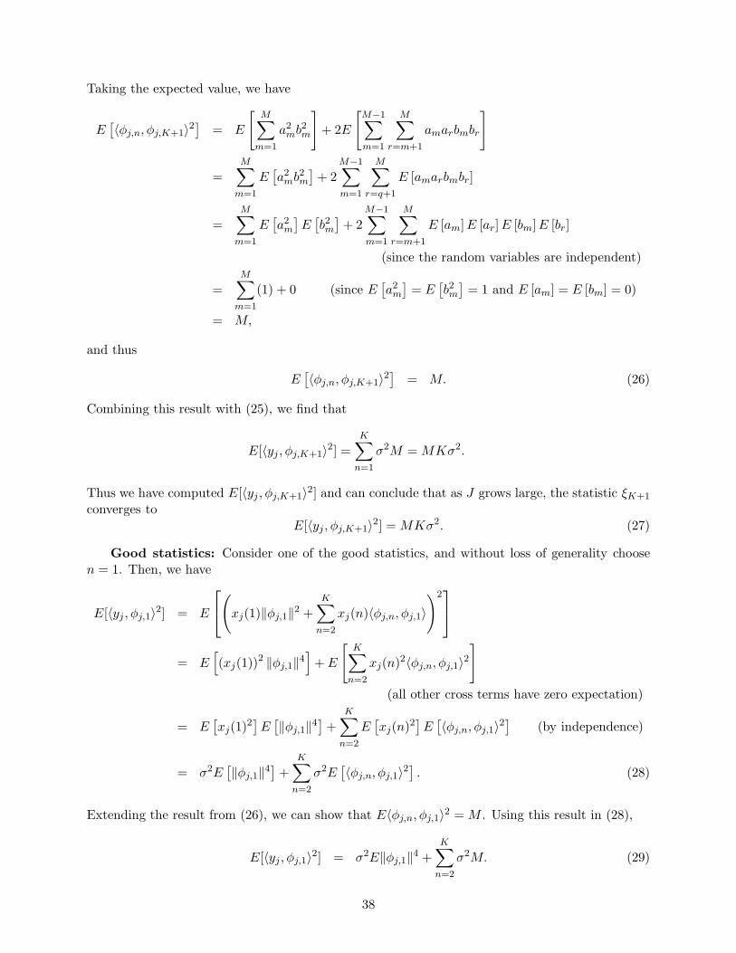
Taking the expected value, we have

E[〈φj,n, φj,K+1〉

2]

= E

[M∑

m=1

a2mb

2m

]+ 2E

[M−1∑

m=1

M∑

r=m+1

amarbmbr

]

=

M∑

m=1

E[a2

mb2m

]+ 2

M−1∑

m=1

M∑

r=q+1

E [amarbmbr]

=

M∑

m=1

E[a2

m

]E[b2m]+ 2

M−1∑

m=1

M∑

r=m+1

E [am]E [ar]E [bm]E [br]

(since the random variables are independent)

=M∑

m=1

(1) + 0 (since E[a2

m

]= E

[b2m]

= 1 and E [am] = E [bm] = 0)

= M,

and thus

E[〈φj,n, φj,K+1〉

2]

= M. (26)

Combining this result with (25), we find that

E[〈yj , φj,K+1〉2] =

K∑

n=1

σ2M = MKσ2.

Thus we have computed E[〈yj , φj,K+1〉2] and can conclude that as J grows large, the statistic ξK+1

converges toE[〈yj , φj,K+1〉

2] = MKσ2. (27)

Good statistics: Consider one of the good statistics, and without loss of generality choosen = 1. Then, we have

E[〈yj , φj,1〉2] = E

(xj(1)‖φj,1‖

2 +K∑

n=2

xj(n)〈φj,n, φj,1〉

)2

= E[(xj(1))

2 ‖φj,1‖4]

+ E

[K∑

n=2

xj(n)2〈φj,n, φj,1〉2

]

(all other cross terms have zero expectation)

= E[xj(1)

2]E[‖φj,1‖

4]+

K∑

n=2

E[xj(n)2

]E[〈φj,n, φj,1〉

2]

(by independence)

= σ2E[‖φj,1‖

4]+

K∑

n=2

σ2E[〈φj,n, φj,1〉

2]. (28)

Extending the result from (26), we can show that E〈φj,n, φj,1〉2 = M . Using this result in (28),

E[〈yj , φj,1〉2] = σ2E‖φj,1‖

4 +K∑

n=2

σ2M. (29)

38

To evaluate E[‖φj,1‖

4], let φj,1 be the column vector [c1, c2, . . . , cM ]T , where the elements of the

vector are random N (0, 1). Define the random variable Z = ‖φj,1‖2 =

∑Mm=1 c

2m. Note that (i)

E[‖φj,1‖

4]

= E[Z2]

and (ii) Z is chi-squared distributed with M degrees of freedom. Thus,E[‖φj,1‖

4]

= E[Z2]

= M(M + 2). Using this result in (29), we have

E[〈yj , φj,1〉2] = σ2M(M + 2) + (K − 1)σ2M

= M(M +K + 1)σ2.

We have computed the variance of 〈yj , φj,1〉 and can conclude that as J grows large, the statisticξ1 converges to

E[〈yj , φj,1〉2] = (M +K + 1)Mσ2. (30)

Conclusion: From (27) and (30) we conclude that

limJ→∞

ξn = E[〈yj , φj,n〉2] =

(M +K + 1)Mσ2, n ∈ ΩKMσ2, n /∈ Ω.

For any M ≥ 1, these values are distinct — their ratio is M+K+1K . Therefore, as J increases we can

distinguish between the two expected values of ξn with overwhelming probability.

I Proof of Theorem 8

Our proof has two parts. First we argue that limJ→∞ zC = zC . Then we show that this impliesvanishing probability of error in recovering each innovation zj .

Part 1: We can write our estimate as

zC =1

JΦT y =

1

J

J∑

j=1

ΦTj yj =

1

J

J∑

j=1

1

Mjσ2j

ΦTj Φjxj =

1

J

J∑

j=1

1

Mjσ2j

Mj∑

m=1

(φRj,m)TφR

j,mxj ,

where φRj,m denotes the m-th row of Φj, that is, the m-th measurement vector for node j. Since

the elements of each Φj are Gaussians with variance σ2j , the product (φR

j,m)TφRj,m has the property

E[(φRj,m)TφR

j,m] = σ2j IN .

It follows thatE[(φR

j,m)TφRj,mxj ] = σ2

jE[xj ] = σ2jE[zC + zj ] = σ2

j zC

and, similarly, that

E

1

Mjσ2j

Mj∑

m=1

(φRj,m)TφR

j,mxj

= zC .

Thus, zC is a sample mean of J independent random variables with mean zC . From the law oflarge numbers, we conclude that limJ→∞ zC = zC .

Part 2: Consider recovery of the innovation zj from the adjusted measurement vector yj = yj −Φj zC . As a recovery scheme, we consider a combinatorial search over all K-sparse index sets drawnfrom 1, 2, . . . , N. For each such index set Ω′, we compute the distance from y to the columnspan of Φj,Ω′, denoted by d(y, colspan(Φj,Ω′)), where Φj,Ω′ is the matrix obtained by sampling thecolumns Ω′ from Φj. (This distance can be measured using the pseudoinverse of Φj,Ω′.)

For the correct index set Ω, we know that d(yj , colspan(Φj,Ω)) → 0 as J → ∞. For any otherindex set Ω′, we know from the proof of Theorem 1 that d(yj , colspan(Φj,Ω′)) > 0. Let

39

ζ := minΩ′ 6=Ω

d(yj , colspan(Φi,Ω′)).

With probability one, ζ > 0. Thus for sufficiently large J , we will have d(yj, colspan(Φj,Ω)) < ζ/2,and so the correct index set Ω can be correctly identified. Since limJ→∞ zC = zC , the innovationestimates zj = zj for each j and for J large enough.

Acknowledgments

Thanks to Emmanuel Candes, Albert Cohen, Ron DeVore, Anna Gilbert, Illya Hicks, RobertNowak, Jared Tanner, and Joel Tropp for informative and inspiring conversations. Special thanksto to Mark Davenport for a thorough critique of the manuscript. MBW thanks his former affiliatedinstitutions Caltech and the University of Michigan, where portions of this work were performed.Final thanks to Ryan King for supercharging our computational capabilities.

References

[1] D. Baron, M. F. Duarte, S. Sarvotham, M. B. Wakin, and R. G. Baraniuk, “An information-theoretic approachto distributed compressed sensing,” in Allerton Conf. Communication, Control, and Computing, (Monticello,IL), Sept. 2005.

[2] M. F. Duarte, S. Sarvotham, D. Baron, M. B. Wakin, and R. G. Baraniuk, “Distributed compressed sensing ofjointly sparse signals,” in Asilomar Conf. Signals, Systems and Computers, (Pacific Grove, CA), Nov. 2005.

[3] M. B. Wakin, S. Sarvotham, M. F. Duarte, D. Baron, and R. G. Baraniuk, “Recovery of jointly sparse signalsfrom few random projections,” in Workshop on Neural Info. Proc. Sys. (NIPS), (Vancouver, Canada), Nov.2005.

[4] M. F. Duarte, S. Sarvotham, D. Baron, M. B. Wakin, and R. G. Baraniuk, “Performance limits for jointly sparsesignals via graphical models,” in Workshop on Sensor, Signal and Information Proc. (SENSIP), (Sedona, AZ),May 2008.

[5] R. A. DeVore, B. Jawerth, and B. J. Lucier, “Image compression through wavelet transform coding,” IEEETrans. Inform. Theory, vol. 38, pp. 719–746, Mar. 1992.

[6] J. Shapiro, “Embedded image coding using zerotrees of wavelet coefficients,” IEEE Trans. Signal Proc., vol. 41,pp. 3445–3462, Dec. 1993.

[7] Z. Xiong, K. Ramchandran, and M. T. Orchard, “Space-frequency quantization for wavelet image coding,” IEEETrans. Image Proc., vol. 6, no. 5, pp. 677–693, 1997.

[8] S. Mallat, A Wavelet Tour of Signal Processing. San Diego: Academic Press, 1999.

[9] K. Brandenburg, “MP3 and AAC explained,” in AES 17th International Conference on High-Quality AudioCoding, Sept. 1999.

[10] W. Pennebaker and J. Mitchell, “JPEG: Still image data compression standard,” Van Nostrand Reinhold, 1993.

[11] D. S. Taubman and M. W. Marcellin, JPEG 2000: Image Compression Fundamentals, Standards and Practice.Kluwer, 2001.

[12] T. M. Cover and J. A. Thomas, Elements of Information Theory. New York: Wiley, 1991.

[13] D. Slepian and J. K. Wolf, “Noiseless coding of correlated information sources,” IEEE Trans. Inform. Theory,vol. 19, pp. 471–480, July 1973.

[14] S. Pradhan and K. Ramchandran, “Distributed source coding using syndromes (DISCUS): Design and construc-tion,” IEEE Trans. Inform. Theory, vol. 49, pp. 626–643, Mar. 2003.

[15] Z. Xiong, A. Liveris, and S. Cheng, “Distributed source coding for sensor networks,” IEEE Signal Proc. Mag.,vol. 21, pp. 80–94, Sept. 2004.

[16] R. Cristescu, B. Beferull-Lozano, and M. Vetterli, “On network correlated data gathering,” in IEEE INFOCOM,(Hong Kong), Mar. 2004.

[17] M. Gastpar, P. L. Dragotti, and M. Vetterli, “The distributed Karhunen-Loeve transform,” IEEE Trans. Inform.Theory, vol. 52, pp. 5177–5196, Dec. 2006.

40

[18] R. Wagner, V. Delouille, H. Choi, and R. G. Baraniuk, “Distributed wavelet transform for irregular sensornetwork grids,” in IEEE Statistical Signal Proc. (SSP) Workshop, (Bordeaux, France), July 2005.

[19] A. Ciancio and A. Ortega, “A distributed wavelet compression algorithm for wireless multihop sensor networksusing lifting,” in IEEE Int. Conf. Acoustics, Speech, Signal Proc. (ICASSP), (Philadelphia), Mar. 2005.

[20] T. Uyematsu, “Universal coding for correlated sources with memory,” in Canadian Workshop Inform. Theory,(Vancouver, Canada), June 2001.

[21] J. Garcia-Frias and W. Zhong, “LDPC codes for compression of multi-terminal sources with hidden Markovcorrelation,” IEEE Communications Letters, vol. 7, pp. 115–117, Mar. 2003.

[22] C. Chen, X. Ji, Q. Dai, and X. Liu, “Slepian-Wolf coding of binary finite memory sources using Burrows Wheelertransform,” in Data Compression Conference, (Snowbird, UT), Mar. 2009.

[23] E. Candes, J. Romberg, and T. Tao, “Robust uncertainty principles: Exact signal reconstruction from highlyincomplete frequency information,” IEEE Trans. Inform. Theory, vol. 52, pp. 489–509, Feb. 2006.

[24] D. Donoho, “Compressed sensing,” IEEE Trans. Inform. Theory, vol. 52, pp. 1289–1306, Apr. 2006.

[25] E. J. Candes, “Compressive sampling,” in International Congress of Mathematicians, vol. 3, (Madrid, Spain),pp. 1433–1452, 2006.

[26] J. Tropp and A. C. Gilbert, “Signal recovery from partial information via orthogonal matching pursuit,” IEEETrans. Info. Theory, vol. 53, pp. 4655–4666, Dec. 2007.

[27] R. G. Baraniuk, M. Davenport, R. A. DeVore, and M. B. Wakin, “A simple proof of the restricted isometryproperty for random matrices,” Constructive Approximation, vol. 28, pp. 253–263, Dec. 2008.

[28] W. U. Bajwa, J. D. Haupt, A. M. Sayeed, and R. D. Nowak, “Joint source-channel communication for distributedestimation in sensor networks,” IEEE Trans. Inform. Theory, vol. 53, pp. 3629–3653, Oct. 2007.

[29] M. Rabbat, J. D. Haupt, A. Singh, and R. D. Nowak, “Decentralized compression and predistribution viarandomized gossiping,” in Int. Workshop on Info. Proc. in Sensor Networks (IPSN), (Nashville, TN), Apr.2006.

[30] W. Wang, M. Garofalakis, and K. Ramchandran, “Distributed sparse random projections for refinable approxi-mation,” in Int. Workshop on Info. Proc. in Sensor Networks (IPSN), (Cambridge, MA), 2007.

[31] S. Aeron, M. Zhao, and V. Saligrama, “On sensing capacity of sensor networks for the class of linear observation,fixed SNR models,” 2007. Preprint.

[32] S. Aeron, M. Zhao, and V. Saligrama, “Fundamental limits on sensing capacity for sensor networks and com-pressed sensing,” 2008. Preprint.

[33] E. Candes and T. Tao, “The Dantzig selector: Statistical estimation when p is much larger than n,” Annals ofStatistics, vol. 35, pp. 2313–2351, Dec. 2007.

[34] S. Sarvotham, D. Baron, and R. G. Baraniuk, “Measurements vs. bits: Compressed sensing meets informationtheory,” in Allerton Conf. Communication, Control, and Computing, (Monticello, IL), Sept. 2006.

[35] E. Candes and D. Donoho, “Curvelets — A surprisingly effective nonadaptive representation for objects withedges,” Curves and Surfaces, 1999.

[36] M. F. Duarte, M. B. Wakin, D. Baron, and R. G. Baraniuk, “Universal distributed sensing via random projec-tions,” in Int. Workshop on Info. Proc. in Sensor Networks (IPSN), (Nashville, TN), Apr. 2006.

[37] “Compressed sensing website.” http://dsp.rice.edu/cs/.

[38] R. Venkataramani and Y. Bresler, “Further results on spectrum blind sampling of 2D signals,” in IEEE Int.Conf. Image Proc. (ICIP), vol. 2, (Chicago), Oct. 1998.

[39] E. Candes, M. Rudelson, T. Tao, and R. Vershynin, “Error correction via linear programming,” in Annual IEEESymposium on Foundations of Computer Science, (Pittsburgh, PA), pp. 295–308, Oct. 2005.

[40] D. Donoho and J. Tanner, “Neighborliness of randomly projected simplices in high dimensions,” Proc. NationalAcademy of Sciences, vol. 102, no. 27, pp. 9452–457, 2005.

[41] D. Donoho, “High-dimensional centrally symmetric polytopes with neighborliness proportional to dimension,”Discrete and Computational Geometry, vol. 35, pp. 617–652, Mar. 2006.

[42] D. L. Donoho and J. Tanner, “Counting faces of randomly projected polytopes when the projection radicallylowers dimension,” Journal of the American Mathematical Society, vol. 22, pp. 1–53, Jan. 2009.

[43] A. Cohen, W. Dahmen, and R. A. DeVore, “Near optimal approximation of arbitrary vectors from highlyincomplete measurements,” 2007. Preprint.

41

[44] D. Needell and R. Vershynin, “Uniform uncertainty principle and signal recovery via regularized orthogonalmatching pursuit,” Dec. 2007. Preprint.

[45] D. Needell and J. Tropp, “CoSaMP: Iterative signal recovery from incomplete and inaccurate samples,” Appliedand Computational Harmonic Analysis, June 2008. To appear.

[46] W. Dai and O. Milenkovic, “Subspace pursuit for compressive sensing: Closing the gap between performanceand complexity,” Mar. 2008. Preprint.

[47] A. Hormati and M. Vetterli, “Distributed compressed sensing: Sparsity models and reconstruction algorithms us-ing anihilating filter,” in IEEE Int. Conf. Acoustics, Speech, Signal Proc. (ICASSP), (Las Vegas, NV), pp. 5141–5144, Apr. 2008.

[48] M. Mishali and Y. Eldar, “Reduce and boost: Recovering arbitrary sets of jointly sparse vectors,” Feb. 2008.Preprint.

[49] M. Fornassier and H. Rauhut, “Recovery algorithms for vector valued data with joint sparsity constrains,” SIAMJournal on Numerical Analysis, vol. 46, no. 2, pp. 577–613, 2008.

[50] R. Gribonval, H. Rauhut, K. Schnass, and P. Vandergheynst, “Atoms of all channels, unite! Average caseanalysis of multi-channel sparse recovery using greedy algorithms,” 2007. Preprint.

[51] D. Estrin, D. Culler, K. Pister, and G. Sukhatme, “Connecting the physical world with pervasive networks,”IEEE Pervasive Computing, vol. 1, no. 1, pp. 59–69, 2002.

[52] G. J. Pottie and W. J. Kaiser, “Wireless integrated network sensors,” Comm. ACM, vol. 43, no. 5, pp. 51–58,2000.

[53] J. Tropp, A. C. Gilbert, and M. J. Strauss, “Simulataneous sparse approximation via greedy pursuit,” in IEEEInt. Conf. Acoustics, Speech, Signal Proc. (ICASSP), (Philadelphia), Mar. 2005.

[54] V. N. Temlyakov, “A remark on simultaneous sparse approximation,” East J. Approx., vol. 100, pp. 17–25, 2004.

[55] S. F. Cotter, B. D. Rao, K. Engan, and K. Kreutz-Delgado, “Sparse solutions to linear inverse problems withmultiple measurement vectors,” IEEE Trans. Signal Proc., vol. 51, pp. 2477–2488, July 2005.

[56] R. Puri and K. Ramchandran, “PRISM: A new robust video coding architecture based on distributed compressionprinciples,” in Allerton Conf. Communication, Control, and Computing, (Monticello, IL), Oct. 2002.

[57] R. Wagner, R. G. Baraniuk, and R. D. Nowak, “Distributed image compression for sensor networks usingcorrespondence analysis and super-resolution,” in Data Comp. Conf. (DCC), Mar. 2000.

[58] C. Weidmann and M. Vetterli, “Rate-distortion analysis of spike processes,” in Data Compression Conference(DCC), (Snowbird, UT), pp. 82–91, Mar. 1999.

[59] D. Baron, M. Duarte, S. Sarvotham, M. B. Wakin, and R. G. Baraniuk, “Distributed compressed sensing,” Tech.Rep. TREE0612, Rice University, Houston, TX, Nov. 2006. Available at http://dsp.rice.edu/cs/.

[60] R. D. Nowak. Personal Communication, 2006.

[61] S. Sarvotham, M. B. Wakin, D. Baron, M. F. Duarte, and R. G. Baraniuk, “Analysis of the DCS one-stagegreedy algoritm for common sparse supports,” Tech. Rep. TREE0503, Rice University, Houston, TX, Oct. 2005.Available at http://www.ece.rice.edu/∼shri/docs/TR0503.pdf.

[62] J. Tropp, “Algorithms for simultaneous sparse approximation. Part II: Convex relaxation,” Signal Proc., vol. 86,pp. 589–602, Mar. 2006.

[63] D. Donoho and Y. Tsaig, “Extensions of compressed sensing,” Signal Proc., vol. 86, pp. 533–548, Mar. 2006.

[64] J. D. Haupt and R. D. Nowak, “Signal reconstruction from noisy random projections,” IEEE Transactions onInformation Theory, vol. 52, pp. 4036–4048, Sept. 2006.

[65] C. Berrou, A. Glavieux, and P. Thitimajshima, “Near Shannon limit error correcting coding and decoding:Turbo codes,” IEEE Int. Conf. Communications, pp. 1064–1070, May 1993.

[66] R. G. Baraniuk, V. Cevher, M. F. Duarte, and C. Hegde, “Model-based compressive sensing,” 2008. Preprint.

[67] P. T. Boufounos and R. G. Baraniuk, “Quantization of sparse representations,” Technical Report TREE0701,Rice University, Houston, TX, Mar. 2007.

[68] A. K. Fletcher, S. Rangan, and V. K. Goyal, “On the rate-distortion performance of compressed sensing,” inIEEE Int. Conf. Acoustics, Speech, Signal Proc. (ICASSP), (Honolulu, HI), pp. III–885–888, Apr. 2007.

[69] E. Candes, J. Romberg, and T. Tao, “Stable signal recovery from incomplete and inaccurate measurements,”Comm. on Pure and Applied Math., vol. 59, pp. 1207–1223, Aug. 2006.

[70] P. T. Boufounos and R. G. Baraniuk, “1-bit compressive sensing,” in Conf. Information Sciences and Systems(CISS), (Princeton, NJ), pp. 16–21, Mar. 2008.

[71] D. B. West, Introduction to Graph Theory. Prentice Hall, 1996.

42