A Tutorial on Compressive Sensing Simon Foucart Drexel University / University of Georgia CIMPA13 New Trends in Applied Harmonic Analysis Mar del Plata, Argentina, 5-16 August 2013

Welcome message from author
This document is posted to help you gain knowledge. Please leave a comment to let me know what you think about it! Share it to your friends and learn new things together.
Transcript
A Tutorial on Compressive Sensing
Simon FoucartDrexel University / University of Georgia
CIMPA13New Trends in Applied Harmonic Analysis
Mar del Plata, Argentina, 5-16 August 2013

This minicourse acts as an invitation to the elegant theory ofCompressive Sensing. It aims at giving a solid overview of thefundamental mathematical aspects. Its content is partly basedon a recent textbook coauthored with Holger Rauhut:

Part 1: The Standard Problem and First Algorithms
The lecture introduces the question of sparse recovery, establishesits theoretical limits, and presents an algorithm achieving theselimits in an idealized situation. In order to treat more realisticsituations, other algorithms are necessary. Basis Pursuit (that is,`1-minimization) and Orthogonal Matching Pursuit make their firstappearance. Their success is proved using the concept ofcoherence of a matrix.

Keywords
I SparsityEssential
I RandomnessNothing better so far
(measurement process)
I OptimizationPreferred, but competitive alternatives are available
(reconstruction process)

Keywords
I SparsityEssential
I RandomnessNothing better so far
(measurement process)
I OptimizationPreferred, but competitive alternatives are available
(reconstruction process)

Keywords
I SparsityEssential
I RandomnessNothing better so far
(measurement process)
I OptimizationPreferred, but competitive alternatives are available
(reconstruction process)

Keywords
I SparsityEssential
I RandomnessNothing better so far
(measurement process)
I OptimizationPreferred, but competitive alternatives are available
(reconstruction process)

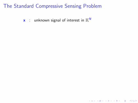
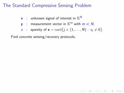
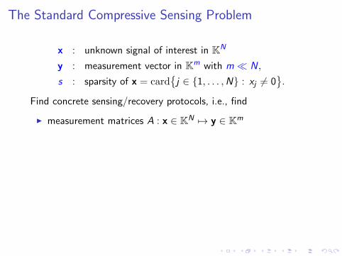
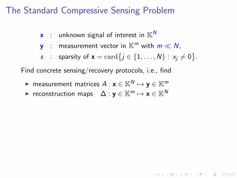
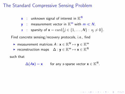
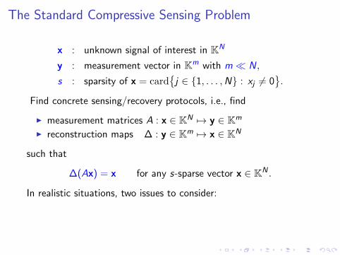
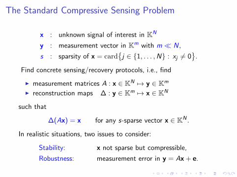
The Standard Compressive Sensing Problem
x : unknown signal of interest in KN
y : measurement vector in Km with m� N,
s : sparsity of x = card{j ∈ {1, . . . ,N} : xj 6= 0
}.
Find concrete sensing/recovery protocols, i.e., find
I measurement matrices A : x ∈ KN 7→ y ∈ Km
I reconstruction maps ∆ : y ∈ Km 7→ x ∈ KN
such that
∆(Ax) = x for any s-sparse vector x ∈ KN .
In realistic situations, two issues to consider:
Stability: x not sparse but compressible,
Robustness: measurement error in y = Ax + e.
The Standard Compressive Sensing Problem
x : unknown signal of interest in KN
y : measurement vector in Km
with m� N,
s : sparsity of x = card{j ∈ {1, . . . ,N} : xj 6= 0
}.
Find concrete sensing/recovery protocols, i.e., find
I measurement matrices A : x ∈ KN 7→ y ∈ Km
I reconstruction maps ∆ : y ∈ Km 7→ x ∈ KN
such that
∆(Ax) = x for any s-sparse vector x ∈ KN .
In realistic situations, two issues to consider:
Stability: x not sparse but compressible,
Robustness: measurement error in y = Ax + e.
The Standard Compressive Sensing Problem
x : unknown signal of interest in KN
y : measurement vector in Km with m� N,
s : sparsity of x = card{j ∈ {1, . . . ,N} : xj 6= 0
}.
Find concrete sensing/recovery protocols, i.e., find
I measurement matrices A : x ∈ KN 7→ y ∈ Km
I reconstruction maps ∆ : y ∈ Km 7→ x ∈ KN
such that
∆(Ax) = x for any s-sparse vector x ∈ KN .
In realistic situations, two issues to consider:
Stability: x not sparse but compressible,
Robustness: measurement error in y = Ax + e.
The Standard Compressive Sensing Problem
x : unknown signal of interest in KN
y : measurement vector in Km with m� N,
s : sparsity of x
= card{j ∈ {1, . . . ,N} : xj 6= 0
}.
Find concrete sensing/recovery protocols, i.e., find
I measurement matrices A : x ∈ KN 7→ y ∈ Km
I reconstruction maps ∆ : y ∈ Km 7→ x ∈ KN
such that
∆(Ax) = x for any s-sparse vector x ∈ KN .
In realistic situations, two issues to consider:
Stability: x not sparse but compressible,
Robustness: measurement error in y = Ax + e.
The Standard Compressive Sensing Problem
x : unknown signal of interest in KN
y : measurement vector in Km with m� N,
s : sparsity of x = card{j ∈ {1, . . . ,N} : xj 6= 0
}.
Find concrete sensing/recovery protocols, i.e., find
I measurement matrices A : x ∈ KN 7→ y ∈ Km
I reconstruction maps ∆ : y ∈ Km 7→ x ∈ KN
such that
∆(Ax) = x for any s-sparse vector x ∈ KN .
In realistic situations, two issues to consider:
Stability: x not sparse but compressible,
Robustness: measurement error in y = Ax + e.
The Standard Compressive Sensing Problem
x : unknown signal of interest in KN
y : measurement vector in Km with m� N,
s : sparsity of x = card{j ∈ {1, . . . ,N} : xj 6= 0
}.
Find concrete sensing/recovery protocols,
i.e., find
I measurement matrices A : x ∈ KN 7→ y ∈ Km
I reconstruction maps ∆ : y ∈ Km 7→ x ∈ KN
such that
∆(Ax) = x for any s-sparse vector x ∈ KN .
In realistic situations, two issues to consider:
Stability: x not sparse but compressible,
Robustness: measurement error in y = Ax + e.
The Standard Compressive Sensing Problem
x : unknown signal of interest in KN
y : measurement vector in Km with m� N,
s : sparsity of x = card{j ∈ {1, . . . ,N} : xj 6= 0
}.
Find concrete sensing/recovery protocols, i.e., find
I measurement matrices A : x ∈ KN 7→ y ∈ Km
I reconstruction maps ∆ : y ∈ Km 7→ x ∈ KN
such that
∆(Ax) = x for any s-sparse vector x ∈ KN .
In realistic situations, two issues to consider:
Stability: x not sparse but compressible,
Robustness: measurement error in y = Ax + e.
The Standard Compressive Sensing Problem
x : unknown signal of interest in KN
y : measurement vector in Km with m� N,
s : sparsity of x = card{j ∈ {1, . . . ,N} : xj 6= 0
}.
Find concrete sensing/recovery protocols, i.e., find
I measurement matrices A : x ∈ KN 7→ y ∈ Km
I reconstruction maps ∆ : y ∈ Km 7→ x ∈ KN
such that
∆(Ax) = x for any s-sparse vector x ∈ KN .
In realistic situations, two issues to consider:
Stability: x not sparse but compressible,
Robustness: measurement error in y = Ax + e.

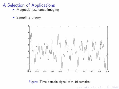
A Selection of Applications
I Magnetic resonance imaging
Figure: Left: traditional MRI reconstruction; Right: compressivesensing reconstruction (courtesy of M. Lustig and S. Vasanawala)
I Sampling theory
0.5 0.4 0.3 0.2 0.1 0 0.1 0.2 0.3 0.4 0.56
4
2
0
2
4
6
8
Figure: Time-domain signal with 16 samples.
I Error correction
I and many more...

A Selection of ApplicationsI Magnetic resonance imaging
Figure: Left: traditional MRI reconstruction; Right: compressivesensing reconstruction (courtesy of M. Lustig and S. Vasanawala)
I Sampling theory
0.5 0.4 0.3 0.2 0.1 0 0.1 0.2 0.3 0.4 0.56
4
2
0
2
4
6
8
Figure: Time-domain signal with 16 samples.
I Error correction
I and many more...
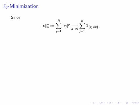
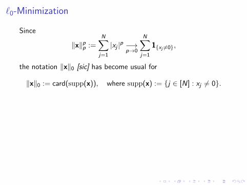
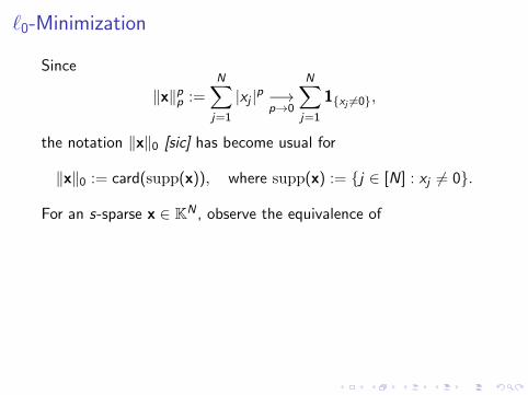
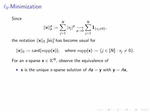
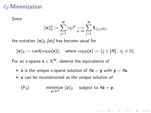
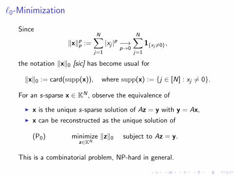
`0-Minimization
Since
‖x‖pp :=N∑j=1
|xj |p −→p→0
N∑j=1
1{xj 6=0},
the notation ‖x‖0 [sic] has become usual for
‖x‖0 := card(supp(x)), where supp(x) := {j ∈ [N] : xj 6= 0}.
For an s-sparse x ∈ KN , observe the equivalence of
I x is the unique s-sparse solution of Az = y with y = Ax,
I x can be reconstructed as the unique solution of
(P0) minimizez∈KN
‖z‖0 subject to Az = y.
This is a combinatorial problem, NP-hard in general.

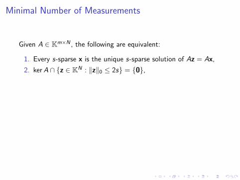
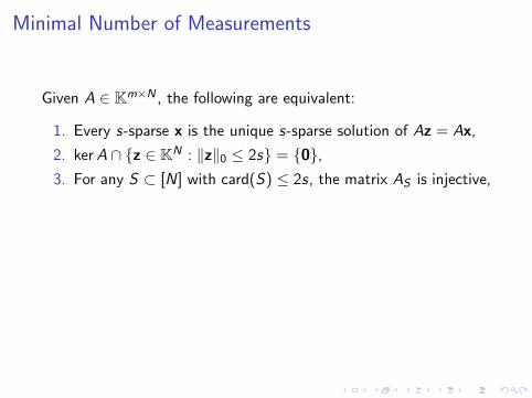
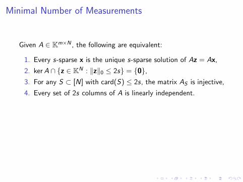
Minimal Number of Measurements
Given A ∈ Km×N , the following are equivalent:
1. Every s-sparse x is the unique s-sparse solution of Az = Ax,
2. kerA ∩ {z ∈ KN : ‖z‖0 ≤ 2s} = {0},3. For any S ⊂ [N] with card(S) ≤ 2s, the matrix AS is injective,
4. Every set of 2s columns of A is linearly independent.
As a consequence, exact recovery of every s-sparse vector forces
m ≥ 2s.
This can be achieved using partial Vandermonde matrices.
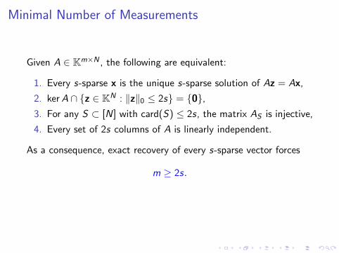
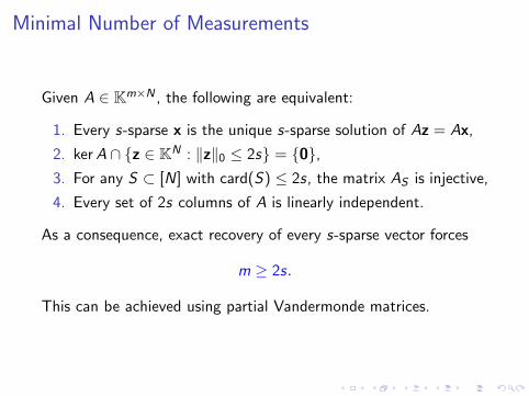
Minimal Number of Measurements
Given A ∈ Km×N , the following are equivalent:
1. Every s-sparse x is the unique s-sparse solution of Az = Ax,
2. kerA ∩ {z ∈ KN : ‖z‖0 ≤ 2s} = {0},
3. For any S ⊂ [N] with card(S) ≤ 2s, the matrix AS is injective,
4. Every set of 2s columns of A is linearly independent.
As a consequence, exact recovery of every s-sparse vector forces
m ≥ 2s.
This can be achieved using partial Vandermonde matrices.
Minimal Number of Measurements
Given A ∈ Km×N , the following are equivalent:
1. Every s-sparse x is the unique s-sparse solution of Az = Ax,
2. kerA ∩ {z ∈ KN : ‖z‖0 ≤ 2s} = {0},3. For any S ⊂ [N] with card(S) ≤ 2s, the matrix AS is injective,
4. Every set of 2s columns of A is linearly independent.
As a consequence, exact recovery of every s-sparse vector forces
m ≥ 2s.
This can be achieved using partial Vandermonde matrices.
Minimal Number of Measurements
Given A ∈ Km×N , the following are equivalent:
1. Every s-sparse x is the unique s-sparse solution of Az = Ax,
2. kerA ∩ {z ∈ KN : ‖z‖0 ≤ 2s} = {0},3. For any S ⊂ [N] with card(S) ≤ 2s, the matrix AS is injective,
4. Every set of 2s columns of A is linearly independent.
As a consequence, exact recovery of every s-sparse vector forces
m ≥ 2s.
This can be achieved using partial Vandermonde matrices.

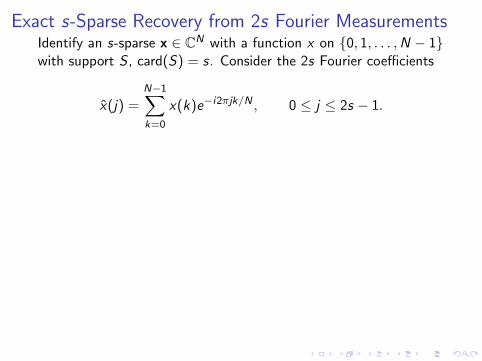
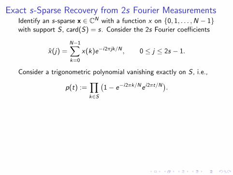
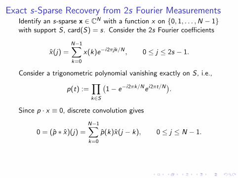
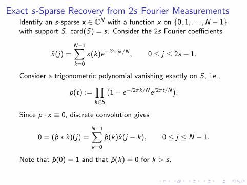
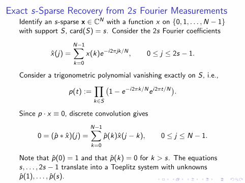
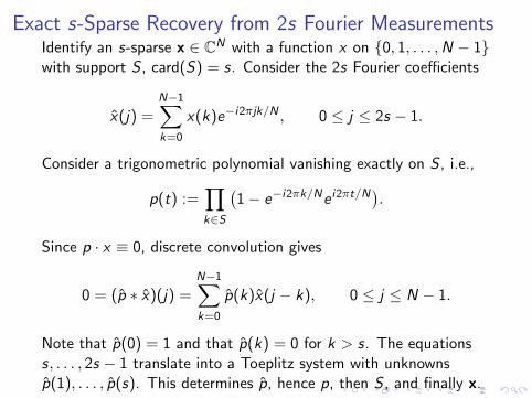
Exact s-Sparse Recovery from 2s Fourier Measurements
Identify an s-sparse x ∈ CN with a function x on {0, 1, . . . ,N − 1}with support S , card(S) = s. Consider the 2s Fourier coefficients
x̂(j) =N−1∑k=0
x(k)e−i2πjk/N , 0 ≤ j ≤ 2s − 1.
Consider a trigonometric polynomial vanishing exactly on S , i.e.,
p(t) :=∏k∈S
(1− e−i2πk/Ne i2πt/N
).
Since p · x ≡ 0, discrete convolution gives
0 = (p̂ ∗ x̂)(j) =N−1∑k=0
p̂(k)x̂(j − k), 0 ≤ j ≤ N − 1.
Note that p̂(0) = 1 and that p̂(k) = 0 for k > s. The equationss, . . . , 2s − 1 translate into a Toeplitz system with unknownsp̂(1), . . . , p̂(s). This determines p̂, hence p, then S , and finally x.

Exact s-Sparse Recovery from 2s Fourier MeasurementsIdentify an s-sparse x ∈ CN with a function x on {0, 1, . . . ,N − 1}with support S , card(S) = s.
Consider the 2s Fourier coefficients
x̂(j) =N−1∑k=0
x(k)e−i2πjk/N , 0 ≤ j ≤ 2s − 1.
Consider a trigonometric polynomial vanishing exactly on S , i.e.,
p(t) :=∏k∈S
(1− e−i2πk/Ne i2πt/N
).
Since p · x ≡ 0, discrete convolution gives
0 = (p̂ ∗ x̂)(j) =N−1∑k=0
p̂(k)x̂(j − k), 0 ≤ j ≤ N − 1.
Note that p̂(0) = 1 and that p̂(k) = 0 for k > s. The equationss, . . . , 2s − 1 translate into a Toeplitz system with unknownsp̂(1), . . . , p̂(s). This determines p̂, hence p, then S , and finally x.
Exact s-Sparse Recovery from 2s Fourier MeasurementsIdentify an s-sparse x ∈ CN with a function x on {0, 1, . . . ,N − 1}with support S , card(S) = s. Consider the 2s Fourier coefficients
x̂(j) =N−1∑k=0
x(k)e−i2πjk/N , 0 ≤ j ≤ 2s − 1.
Consider a trigonometric polynomial vanishing exactly on S , i.e.,
p(t) :=∏k∈S
(1− e−i2πk/Ne i2πt/N
).
Since p · x ≡ 0, discrete convolution gives
0 = (p̂ ∗ x̂)(j) =N−1∑k=0
p̂(k)x̂(j − k), 0 ≤ j ≤ N − 1.
Note that p̂(0) = 1 and that p̂(k) = 0 for k > s.
The equationss, . . . , 2s − 1 translate into a Toeplitz system with unknownsp̂(1), . . . , p̂(s). This determines p̂, hence p, then S , and finally x.
Exact s-Sparse Recovery from 2s Fourier MeasurementsIdentify an s-sparse x ∈ CN with a function x on {0, 1, . . . ,N − 1}with support S , card(S) = s. Consider the 2s Fourier coefficients
x̂(j) =N−1∑k=0
x(k)e−i2πjk/N , 0 ≤ j ≤ 2s − 1.
Consider a trigonometric polynomial vanishing exactly on S , i.e.,
p(t) :=∏k∈S
(1− e−i2πk/Ne i2πt/N
).
Since p · x ≡ 0, discrete convolution gives
0 = (p̂ ∗ x̂)(j) =N−1∑k=0
p̂(k)x̂(j − k), 0 ≤ j ≤ N − 1.
Note that p̂(0) = 1 and that p̂(k) = 0 for k > s. The equationss, . . . , 2s − 1 translate into a Toeplitz system with unknownsp̂(1), . . . , p̂(s).
This determines p̂, hence p, then S , and finally x.
Exact s-Sparse Recovery from 2s Fourier MeasurementsIdentify an s-sparse x ∈ CN with a function x on {0, 1, . . . ,N − 1}with support S , card(S) = s. Consider the 2s Fourier coefficients
x̂(j) =N−1∑k=0
x(k)e−i2πjk/N , 0 ≤ j ≤ 2s − 1.
Consider a trigonometric polynomial vanishing exactly on S , i.e.,
p(t) :=∏k∈S
(1− e−i2πk/Ne i2πt/N
).
Since p · x ≡ 0, discrete convolution gives
0 = (p̂ ∗ x̂)(j) =N−1∑k=0
p̂(k)x̂(j − k), 0 ≤ j ≤ N − 1.
Note that p̂(0) = 1 and that p̂(k) = 0 for k > s. The equationss, . . . , 2s − 1 translate into a Toeplitz system with unknownsp̂(1), . . . , p̂(s). This determines p̂, hence p, then S , and finally x.

Optimization and Greedy Strategies

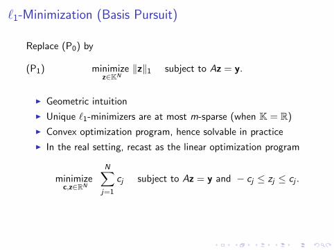
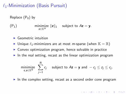
`1-Minimization (Basis Pursuit)
Replace (P0) by
(P1) minimizez∈KN
‖z‖1 subject to Az = y.
I Geometric intuition
I Unique `1-minimizers are at most m-sparse (when K = R)
I Convex optimization program, hence solvable in practice
I In the real setting, recast as the linear optimization program
minimizec,z∈RN
N∑j=1
cj subject to Az = y and − cj ≤ zj ≤ cj .
I In the complex setting, recast as a second order cone program

Basis Pursuit — Null Space Property
∆1(Ax) = x for every vector x supported on S if and only if
(NSP) ‖uS‖1 < ‖uS‖1, all u ∈ kerA \ {0}.
For real measurement matrices, real and complex NSPs read∑j∈S|uj | <
∑`∈S
|u`|, all u ∈ kerR A \ {0},
∑j∈S
√v2j + w2
j <∑`∈S
√v2` + w2
` , all (v,w) ∈ (kerR A)2 \ {0}.
Real and complex NSPs are in fact equivalent.

Basis Pursuit — Null Space Property
∆1(Ax) = x for every vector x supported on S if and only if
(NSP) ‖uS‖1 < ‖uS‖1, all u ∈ kerA \ {0}.
For real measurement matrices,
real and complex NSPs read∑j∈S|uj | <
∑`∈S
|u`|, all u ∈ kerR A \ {0},
∑j∈S
√v2j + w2
j <∑`∈S
√v2` + w2
` , all (v,w) ∈ (kerR A)2 \ {0}.
Real and complex NSPs are in fact equivalent.

Basis Pursuit — Null Space Property
∆1(Ax) = x for every vector x supported on S if and only if
(NSP) ‖uS‖1 < ‖uS‖1, all u ∈ kerA \ {0}.
For real measurement matrices, real and complex NSPs read
∑j∈S|uj | <
∑`∈S
|u`|, all u ∈ kerR A \ {0},
∑j∈S
√v2j + w2
j <∑`∈S
√v2` + w2
` , all (v,w) ∈ (kerR A)2 \ {0}.
Real and complex NSPs are in fact equivalent.

Basis Pursuit — Null Space Property
∆1(Ax) = x for every vector x supported on S if and only if
(NSP) ‖uS‖1 < ‖uS‖1, all u ∈ kerA \ {0}.
For real measurement matrices, real and complex NSPs read∑j∈S|uj | <
∑`∈S
|u`|, all u ∈ kerR A \ {0},
∑j∈S
√v2j + w2
j <∑`∈S
√v2` + w2
` , all (v,w) ∈ (kerR A)2 \ {0}.
Real and complex NSPs are in fact equivalent.

Basis Pursuit — Null Space Property
∆1(Ax) = x for every vector x supported on S if and only if
(NSP) ‖uS‖1 < ‖uS‖1, all u ∈ kerA \ {0}.
For real measurement matrices, real and complex NSPs read∑j∈S|uj | <
∑`∈S
|u`|, all u ∈ kerR A \ {0},
∑j∈S
√v2j + w2
j <∑`∈S
√v2` + w2
` , all (v,w) ∈ (kerR A)2 \ {0}.
Real and complex NSPs are in fact equivalent.

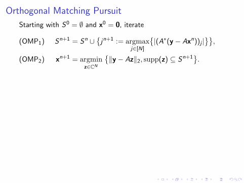
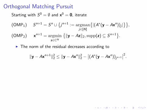
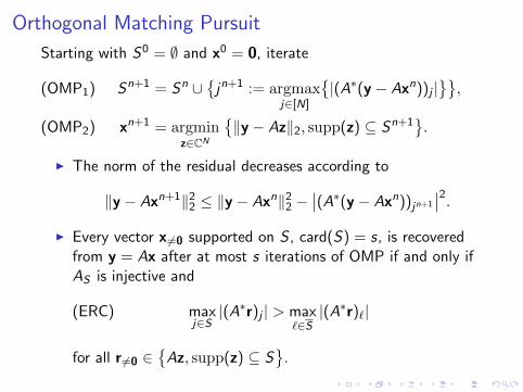
Orthogonal Matching Pursuit
Starting with S0 = ∅ and x0 = 0, iterate
Sn+1 = Sn ∪{jn+1 := argmax
j∈[N]
{|(A∗(y − Axn))j |
}},(OMP1)
xn+1 = argminz∈CN
{‖y − Az‖2, supp(z) ⊆ Sn+1
}.(OMP2)
I The norm of the residual decreases according to
‖y − Axn+1‖22 ≤ ‖y − Axn‖22 −∣∣(A∗(y − Axn))jn+1
∣∣2.I Every vector x 6=0 supported on S , card(S) = s, is recovered
from y = Ax after at most s iterations of OMP if and only ifAS is injective and
(ERC) maxj∈S|(A∗r)j | > max
`∈S|(A∗r)`|
for all r 6=0 ∈{Az, supp(z) ⊆ S
}.
Orthogonal Matching Pursuit
Starting with S0 = ∅ and x0 = 0, iterate
Sn+1 = Sn ∪{jn+1 := argmax
j∈[N]
{|(A∗(y − Axn))j |
}},(OMP1)
xn+1 = argminz∈CN
{‖y − Az‖2, supp(z) ⊆ Sn+1
}.(OMP2)
I The norm of the residual decreases according to
‖y − Axn+1‖22 ≤ ‖y − Axn‖22 −∣∣(A∗(y − Axn))jn+1
∣∣2.
I Every vector x 6=0 supported on S , card(S) = s, is recoveredfrom y = Ax after at most s iterations of OMP if and only ifAS is injective and
(ERC) maxj∈S|(A∗r)j | > max
`∈S|(A∗r)`|
for all r 6=0 ∈{Az, supp(z) ⊆ S
}.
Orthogonal Matching Pursuit
Starting with S0 = ∅ and x0 = 0, iterate
Sn+1 = Sn ∪{jn+1 := argmax
j∈[N]
{|(A∗(y − Axn))j |
}},(OMP1)
xn+1 = argminz∈CN
{‖y − Az‖2, supp(z) ⊆ Sn+1
}.(OMP2)
I The norm of the residual decreases according to
‖y − Axn+1‖22 ≤ ‖y − Axn‖22 −∣∣(A∗(y − Axn))jn+1
∣∣2.I Every vector x 6=0 supported on S , card(S) = s, is recovered
from y = Ax after at most s iterations of OMP if and only ifAS is injective and
(ERC) maxj∈S|(A∗r)j | > max
`∈S|(A∗r)`|
for all r 6=0 ∈{Az, supp(z) ⊆ S
}.

First Recovery Guarantees

Coherence
For a matrix with `2-normalized columns a1, . . . , aN , define
µ := maxi 6=j|〈ai , aj〉| .
As a rule, the smaller the coherence, the better.
However, the Welch bound reads
µ ≥
√N −m
m(N − 1).
I Welch bound achieved at and only at equiangular tight frames
I Deterministic matrices with coherence µ ≤ c/√m exist

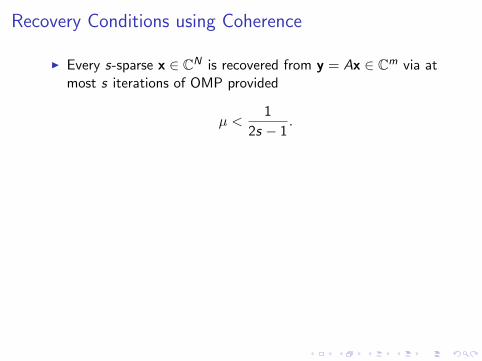
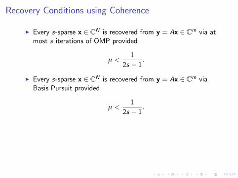
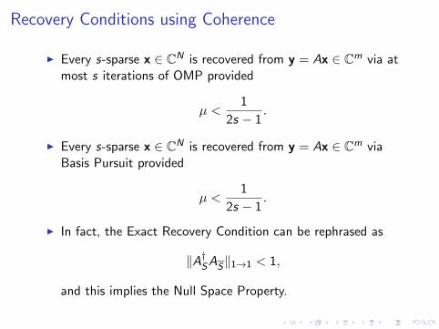
Recovery Conditions using Coherence
I Every s-sparse x ∈ CN is recovered from y = Ax ∈ Cm via atmost s iterations of OMP provided
µ <1
2s − 1.
I Every s-sparse x ∈ CN is recovered from y = Ax ∈ Cm viaBasis Pursuit provided
µ <1
2s − 1.
I In fact, the Exact Recovery Condition can be rephrased as
‖A†SAS‖1→1 < 1,
and this implies the Null Space Property.

Summary
The coherence conditions for s-sparse recovery are of the type
µ ≤ c
s,
while the Welch bound (for N ≥ 2m, say) reads
µ ≥ c√m.
Therefore, arguments based on coherence necessitate
m ≥ c s2.
This is far from the ideal linear scaling of m in s...
Next, we will introduce new tools to break this quadratic barrier(with random matrices).
Related Documents