1 DISSERTATION THE INFLUENCE OF CLIMATE ON TERRESTRIAL CO 2 FLUXES Submitted by Kevin Michael Schaefer Department of Atmospheric Science In partial fulfillment of the requirements for the degree of Doctor of Philosophy Colorado State University Fort Collins, Colorado Summer 2004

Welcome message from author
This document is posted to help you gain knowledge. Please leave a comment to let me know what you think about it! Share it to your friends and learn new things together.
Transcript

1
DISSERTATION
THE INFLUENCE OF CLIMATE ON TERRESTRIAL CO2 FLUXES
Submitted by
Kevin Michael Schaefer
Department of Atmospheric Science
In partial fulfillment of the requirements
for the degree of Doctor of Philosophy
Colorado State University
Fort Collins, Colorado
Summer 2004

2
COLORADO STATE UNIVERSITY
June 1, 2004
WE HEREBY RECOMMEND THE DISSERTATION PREPARED UNDER
OUR SUPERVISION BY KEVIN MICHAEL SCHAEFER ENTITLED THE
INFLUENCE OF CLIMATE ON TERRESTRIAL CO2 FLUXES BE ACCEPTED AS
FULFILLING IN PART REQUIREMENTS FOR THE DEGREE OF DOCTOR OF
PHILOSOPHY.
Committee on Graduate Work
______________________________________
______________________________________
______________________________________
______________________________________
______________________________________
______________________________________ Advisor
______________________________________ Department Head

3
ABSTRACT OF DISSERTATION
THE INFLUENCE OF CLIMATE ON TERRESTRIAL CO2 FLUXES
The concentration of CO2 in the atmosphere ([CO2]) is increasing at only about
half the rate expected based on fossil fuel emissions. This "missing sink" is highly
variable due primarily to the effects of climate variability on terrestrial CO2 fluxes in the
northern hemisphere. Using a series of model simulations, we studied how climate
influences inter-annual variability and long-term trends in terrestrial CO2 fluxes. We
modeled Net Ecosystem Exchange (NEE) of CO2 from 1958-2002 (45 years) using the
Simple Biosphere model, Version 2 (SiB2). As input weather, we used the National
Centers for Environmental Prediction (NCEP) reanalysis and the European Centre for
Medium-range Weather Forecasts (ECMWF) Reanalysis. To define the Leaf Area Index,
we used the Fourier-Adjustment, Solar zenith angle corrected, Interpolated Reconstructed
(FASIR) Normalized Difference Vegetation Index (NDVI) dataset. We used
correlations, trends, and other statistical techniques to isolate the relationships between
NEE and climate.
The simulated NEE reproduces the salient features and magnitude of the
measured global CO2 growth rate. The northern hemisphere shows a pattern of
alternating positive and negative NEE anomalies that cancel such that the tropics
dominate the global simulated NEE inter-annual variability.
Climate influences on NEE have strong regional differences with precipitation
dominating in the tropics and temperature in the extra-tropics. In tropical regions with
drier soils, precipitation control of photosynthesis (i.e., drought stress) dominates. By
contrast, in moist soils, precipitation control of respiration dominates. Due to

4
cancellation and competing effects, no single climate variable controls global or regional
NEE inter-annual variability. Globally, precipitation accounts for 44% of NEE
variability; followed by Leaf Area Index (23%), soil carbon (12%), and temperature
(16%). The influence of ENSO is consistent with that expected for shifting precipitation
patterns in the tropics.
The AO strongly influences autumn, winter, and spring NEE through its influence
on temperature. Soil retains the AO temperature signal for many months, influencing
respiration fluxes well into spring. Seasonally asymmetric NEE trends influence the
seasonal amplitude of atmospheric CO2 concentration. Positive AO polarity in winter
advances the date of leaf out, increasing the spring drawdown of atmospheric CO2.
Positive AO polarity in winter increases temperature and respiration, increasing the
winter buildup of atmospheric CO2. The influence of the AO on summer NEE is minimal
except for North America in August.
The trend in the winter AO partially explains observed trends towards warmer
winters and earlier springs. The timing of spring correlates with the AO where the AO
influences temperature (Eurasia and southeast United States). Modeled trends in leaf out,
snowmelt, and soil thaw are consistent with observations. The AO shows a statistically
significant influence on spring trends in the eastern United States and northern Europe.
Seasonally asymmetric trends in NEE can partially explain the observed trend towards
larger seasonal amplitudes in [CO2]. The components of the land surface with climate
memory (plant buds, snow pack, and soil temperature) integrate the noisy AO input over
time to control the transition from winter to spring.

5
In summary, climatic memory is very important in the study of seasonal dynamics
and that the winter AO influences the transition from winter to spring.
Kevin Michael Schaefer Department of Atmospheric Science Colorado State University Fort Collins, CO 80523 Summer 2004
6
Acknowledgements
I would not have been able to complete this research and obtain an advanced
degree without the love, support, and sacrifice of my wife, Susan Maroney. I thank my
advisor Scott Denning for keeping me focused. I thank my committee members for their
sound advice. I thank all the members of my research group, who at various times
provided help, technical support, data, and encouragement as needed. We thank the
National Oceanic and Atmospheric Administration, Climate Monitoring and Diagnostics
Laboratory, Boulder, Colorado for supplying observations of CO2 concentration. We
thank David Thompson of the Atmospherics Sciences Department, Colorado State
University for valuable advice and insight regarding our analysis of the Arctic
Oscillation. Lastly, I thank my son Jason, who just doesn't care whether Dad has a
graduate degree or not.
This research was funded by NASA under NASA Grant NCC5-621 Supplement
1, through the University of California at Berkeley under NASA grant SA2805-23941,
through the University of California at Santa Barbara under NASA Cooperative
Agreement NCC5-302, the Earth System Science Workbench (ESSW): a scalable
infrastructure for Earth Science Information Partners (ESIPs). Partial funding was also
provided through the Monfort Professor Award from CSU.

7
Table of Contents
ABSTRACT OF DISSERTATION........................................................................ 3
Acknowledgements ................................................................................................. 6
Table of Contents.................................................................................................... 7
1. Introduction..................................................................................................... 9
2. Hypotheses.................................................................................................... 12
3. Methods......................................................................................................... 23
3.1 General.................................................................................................. 23
3.2 SiB Input ............................................................................................... 24
3.3 GPP and Respiration in SiB2 ................................................................ 26
3.4 Statistics ................................................................................................ 41
4. The effect of climate on inter-annual variability of terrestrial CO2 fluxes ... 43
4.1 Introduction and Methods ..................................................................... 43
4.2 NEE Variability..................................................................................... 45
4.3 Climate Influences ................................................................................ 47
4.4 The Arctic Oscillation and NEE Variability......................................... 52
4.5 ENSO and NEE Variability .................................................................. 54
4.6 Conclusions ........................................................................................... 56
5. The winter Arctic Oscillation, the timing of spring, and carbon fluxes in the
northern hemisphere.......................................................................................................... 59
5.1 Introduction and Methods ..................................................................... 59
5.2 Results ................................................................................................... 62
5.3 Conclusions ........................................................................................... 74

8
6. Conclusions and Discussion ......................................................................... 77
6.1 Conclusions ........................................................................................... 77
6.2 Discussion............................................................................................. 80
6.3 Future Research..................................................................................... 80
7. References ..................................................................................................... 83

9
1. Introduction
The observed atmospheric CO2 growth rate over the past 50 years is only about
half that expected based on fossil fuel emissions. Modeling, isotope, and inversion
studies place much of this “missing sink” in the northern hemisphere terrestrial
biosphere, but its spatial distribution and the mechanisms that drive it are not well known.
Predicting future climate requires a deep understanding of how the atmospheric CO2
concentration will respond under various climate change scenarios, which, in turn,
requires an understanding of the mechanisms that drive the missing sink.
The atmospheric CO2 growth rate shows a great deal of inter-annual variability
[Conway et al., 1994; LLoyd, 1999; Rayner and Law, 1999; Tans and Wallace, 1999;
Bousquet et al., 2000; Fung, 2000]. The ocean fluxes show relatively low variability
[Rayner and Law, 1999; Le Quéré et al., 2000], so the growth rate variability is attributed
primarily to changes in the terrestrial sink [Sarmiento, 1993; Conway et al., 1994; Trolier
et al., 1996; Kaduk and Heimann, 1997; LLoyd, 1999; Houghton et al., 1998; Tans and
Wallace, 1999; Houghton, 2000; Prince et al., 2000]. Climate, land use change, natural
disturbance, CO2 fertilization, and nitrogen deposition also influence terrestrial CO2
fluxes [Conway et al., 1994; Bousquet et al., 2000; Fung, 2000; Houghton, 2000], but
climate contributes most to inter-annual variability [Houghton, 2000].
We need to understand how climate variability affects terrestrial CO2 fluxes so
that we can isolate the location and mechanisms behind the missing sink. In addition, the
growth rate variability provides clues about how the biosphere might respond under
various climate change scenarios. Studying how climate influences terrestrial CO2 fluxes
will allow us to test the performance of predictive models under various climate

10
conditions. Lastly, we need accurate estimates of seasonal and inter-annual variability in
CO2 fluxes to serve as background for data assimilation and transport inversion studies
designed to isolate the location and mechanisms behind the missing sink. Until we can
successfully reproduce past variability in the missing sink, the uncertainty in predicting a
future response will remain high.
Lacking direct measurements of net global CO2 fluxes, the scientific community
estimates net terrestrial fluxes from satellite data, inversions, and models. Satellite data,
e.g., the Normalized Difference Vegetation Index (NDVI), is used to estimate the Leaf
Area Index (LAI), which, in combination with a model, is used to estimate global net
primary production [e.g., Goetz et al., 2000 and Ichii et al., 2001]. NDVI does not
contain direct information about respiration, and so we cannot use it alone to estimate net
terrestrial fluxes. Inversions can estimate net fluxes for large, continental scale regions,
but cannot isolate the exact causes of variability [e.g., Bousquet et al., 2000]. Terrestrial
carbon models range from highly mechanistic biogeochemical process models to
statistical regression and bookkeeping models. Biogeochemistry models track the
amount of carbon in various biological pools [e.g., Ichii et al., 2001], but vary widely in
the number of pools and how explicitly they represent photosynthesis and respiration
processes.
My research focused on how climate influences inter-annual variability net
terrestrial CO2 fluxes. We neglected the influence of CO2 fertilization and nitrogen
deposition because they show little inter-annual variability [Houghton, 2000]. CO2
fertilization and nitrogen deposition probably influence long-term trends in the terrestrial
carbon sink, but we are studying the inter-annual variability rather than the magnitude of

11
the terrestrial sink. We also neglected variability due to fossil fuel emissions, which was
small compared to other factors [Houghton, 2000]. Due to time constraints, we did not
consider variability in ocean uptake. CO2 fluxes resulting from land use change, such as
deforestation, are spread over several years, resulting in a relatively low influence on
inter-annual variability in terrestrial CO2 fluxes [Houghton, 2000]. Variability of large-
scale disturbances, such as fires, influences inter-annual variability in terrestrial CO2
fluxes, but are also related to variability in climate [Houghton, 2000]. Although we did
not explicitly isolate the effects of land use change and disturbances, we did not
completely neglect them. The global NDVI dataset used as input to our model includes
the effects of land use change and disturbances.
This dissertation is based on two papers written for journal publication. Chapter 2
(Methods) describes the models, data, and statistical techniques common to both papers.
Chapter 3, the effect of climate on inter-annual variability of terrestrial CO2 fluxes, has
already been published [Schaefer et al., 2002]. Chapter 4, the winter Arctic Oscillation,
the timing of spring, and carbon fluxes in the northern hemisphere, will be submitted to
Global Biogeochemical Cycles. Both chapters include descriptions of models and
techniques unique to each paper.
I posed several specific hypotheses related to the relationship between climate and
NEE and tested them against the model output using various statistical techniques. These
long, global simulations (ranging from 1 to 45 years) can help answer many questions
about the interaction between climate and terrestrial CO2 fluxes. I focused on regional
climate influences, with a strong emphasis on the northern hemisphere because that is the
suspected location of the missing sink.

12
2. Hypotheses
Hypothesis 1: the climate influence on NEE has strong regional differences.
We hypothesize that climate influences on NEE have strong regional differences.
Past studies suggest temperature and precipitation can explain NEE inter-annual
variability, but disagree on the exact mechanism [e.g., Kaduk and Heimann, 1997; LLoyd,
1999; Dickinson, 2000; Houghton, 2000]. Respiration dominates flux inter-annual
variability in some areas [Houghton, 2000] and photosynthesis in others [Kaduk and
Heimann, 1997]. How available light and humidity influence inter-annual variability in
CO2 fluxes are not well known. To test our hypothesis, we will create specialized model
diagnostics (described below) that will allow us to statistically quantify how strongly
each climate factor influences NEE inter-annual variability.
Hypothesis 2: ENSO influences NEE in the tropics
We hypothesize that the El Niño-Southern Oscillation (ENSO) influences NEE in
the tropics. ENSO is the dominant mode of climate variability in the tropical regions and
should account for some of the inter-annual variability in NEE. To test our hypothesis,
we will represent ENSO using the Southern Oscillation Index (SOI) based on the sea
level pressure difference between Tahiti and Darwin. We will then use correlations and
regressions to relate the ENSO to our modeled NEE, respiration, and GPP.
Hypothesis 3: the AO influences NEE in the high northern latitudes
The Arctic Oscillation (AO) is the dominant atmospheric circulation mode in the
northern hemisphere in winter [Thompson et al., 2000]. The AO is a zonally symmetric
seesaw in atmospheric mass between the Arctic and mid-latitudes centered on 45N

13
[Thompson and Wallace, 2000]. Positive AO polarity has less mass and lower pressure
in the Arctic and more mass and higher pressure at 45N. Positive AO polarity is
characterized by westerly geostrophic surface winds along 55N latitude [Thompson and
Wallace, 2001]. This geostrophic balance results in a north-south dipole in the strength
of the zonal wind between 25°N and 60°N [Thompson and Wallace, 2000]. Positive AO
polarity has stronger westerly winds (positive anomalies) north of 45°N and weaker
winds (negative anomalies) south of 45°N [Thompson and Wallace, 2000; Thompson and
Wallace, 2001]. The variance in zonal mean wind due to the AO peaks between 25-35N
and 55-60N latitude [Thompson and Wallace, 2000]. The AO exists all year round, but is
strongest and most variable in winter, when radiative cooling over the pole is greatest and
the polar vortex is strongest. In March, the AO weakens as increased convection over
land breaks down the polar vortex. Since the 1950s, the winter AO has tended towards
positive polarity [Thompson et al., 2000], indicating a gradual strengthening of the
wintertime polar vortex [Serreze et al., 2000].
To represent the AO, we used an index based on the first principle component of
sea level pressure from the National Centers for Environmental Prediction (NCEP)
reanalysis [Thompson and Wallace, 2000]. Because they are highly correlated, we will
use this AO index to also represent the North Atlantic Oscillation (NAO). To visualize
the influence of the AO on climate, we correlated the AO index and the NCEP surface air
temperature and precipitation for winter and early spring (January-February-March or
JFM) for 1958-2002 (Figure 1). Smoother zonal flow associated with positive AO
polarity favors advection of warm, moist oceanic air deep into continental interiors,
resulting in higher temperatures and increased precipitation [Thompson and Wallace,

14
2000]. Warm air advection reduces precipitation in Eurasia south of 55º N latitudes,
resulting in negative precipitation correlations. Positive AO polarity also decreases the
number of cold air outbreaks, resulting in positive temperature anomalies in central North
America [Thompson and Wallace, 2001]. Alaska and Northeast Canada show negative
temperature and precipitation correlations, consistent with cold, dry airflow from the
Arctic expected for positive AO polarity [Thompson and Wallace, 2000]. The AO
randomly switches polarity with a characteristic synoptic time scale of 7-10 days.
We hypothesize that the Arctic Oscillation (AO) influences NEE variability in the
high northern latitudes. To test our hypothesis, we correlated and regressed the AO index
to our modeled NEE, respiration, and GPP. We assessed the influence of the AO on NEE
throughout the year, not just in winter when the AO is strongest. The AO influence on
temperature is stronger than its influence on precipitation, so we expect to see increased
respiration and GPP in those regions where the AO exerts the strongest influence on the
surface air temperature.
Hypothesis 4: Climate memory allows the winter AO to influence spring NEE
We hypothesize that elements of the land surface have sufficient climate memory
such that the winter AO influences variability in spring and early summer NEE. Climate
memory occurs when a slowly changing land component integrates noisy, high frequency
climate variability into a persistent, low frequency signal. The components of the land
system with climate memory include the soil temperature, soil moisture, the snow, and
the plants themselves.
To test our hypothesis, we correlated the winter (JFM) AO index with our
modeled fluxes at various lag times. Since the AO most strongly influences temperature,

15
we expect the soil to retain the winter AO temperature anomaly, influencing respiration
fluxes into spring.
Hypothesis 5: the winter AO influences variability and trends in the timing of spring
We hypothesize that the winter AO, through its influence on temperature and
precipitation, influences the timing of spring in the northern hemisphere. Those
components of the land system with climate memory (soil temperature and moisture,
snow, and plants) control the transition from winter to spring by integrating the noisy
climate input throughout the winter. Events that typically mark the start of spring include
snowmelt, soil thaw, and plant leaf out or flowering. Plant phenophases (i.e., climate
driven growth or senescence events) mark the start and end of the growing season
[Schwartz and Reiter, 2000; Chen and Pan, 2002].
The date of spring depends on the cumulative effects of climate over the entire
winter. The date of snowmelt, for example, depends on snow depth, temperature, and
cloud cover [Dye, 2002; Stone et al., 2002]. Increased precipitation in winter (October-
February) increases snow depth and delays snowmelt by increasing the total energy
required for melting [Cutforth et al., 1999; Vaganov et al., 1999; Stone et al., 2002].
Warmer temperatures in spring (March-May) advance snow melt by increasing melting
and sublimation rates [Stone et al., 2002]. Increased cloudiness in spring (March-May)
advances snowmelt by enhancing cloud thermal forcing from absorbed downwelling
longwave radiation [Stone et al., 2002].
Past research has identified some regional relationships between the timing of
spring and the NAO. The NAO negatively correlates with spring leafing and flowering
(positive NAO means earlier spring), indicating the NAO influence on winter

16
temperatures and precipitation influence spring phenology in Europe. Winter
temperatures and the JFM NAO statistically explain most of the observed variability in
spring phenophases in Europe [D'Odorico et al., 2002; Menzel, 2003]. D'Odorico et al.,
[2002] found that positive AO polarity in winter advanced ice breakup in European rivers
and Lakes. However, we hypothesize that the winter AO influences the timing of spring
throughout the northern hemisphere, not just in Europe.
Various observations over the last half of the 20th century indicate large-scale
climatic trends towards warmer and earlier springs in the northern hemisphere [Serreze et
al., 2000]. Bud burst, leaf out, and other plant phenophases have occurred earlier in
spring, also indicating a longer growing season [Menzel and Fabian, 1999; Keyser et al.,
2000; Menzel, 2000; Menzel, 2003]. Winter and spring temperatures have increased,
spring snow depth and snow cover have decreased, and the date of snowmelt has
advanced [Serreze et al., 2000]. During the same time period, the AO has tended towards
positive polarity during winter [Thompson et al., 2000]. Although the AO pattern
dominates the northern hemisphere [Serreze et al., 2000], how the AO influences
terrestrial carbon fluxes is unclear [Reichenau and Esser, 2003; Schaefer et al., 2002].
Warmer temperatures in early spring have advanced observed leaf unfolding and
flowering in Europe and North America since the 1950s [Menzel and Fabian, 1999;
Keyser et al., 2000; Menzel, 2000; Schwartz and Reiter, 2000; Menzel, 2003]. From
1959-1996 in Europe, the average growing season has increased by 10.8 days [Menzel
and Fabian, 1999; Menzel, 2000]. Since early spring phenophases show the strongest
trends, the longer growing seasons are due primarily to earlier starts in spring [Menzel
and Fabian, 1999; Menzel, 2000]. Trends in autumn phenophases are not as clear, with

17
some species advancing and others retreating, but overall show delays of 4.8 days in
Europe [Menzel and Fabian, 1999; Menzel, 2000; Menzel, 2003]. The inconsistent
autumn trends may result from conflicting temperature influences: higher spring and
early summer temperatures advance leaf coloring while higher autumn temperatures
delay leaf coloring [Menzel, 2003].
Since the 1950s, high latitude winter snow depths have declined and spring snow
cover has decreased 10% [Hartley and Robinson, 2000; Serreze et al., 2000; Dye, 2002;
Stone et al., 2002]. Also, the spring temperature and cloud cover have increased [Stone
et al., 2002], advancing the date of snowmelt [Cutforth et al., 1999; Zhou et al., 2001;
Dye, 2002]. Based on station measurements and NOAA snow charts derived from visible
reflectances, the Week of Last Snow in the northern hemisphere spring has advanced 9-
15 days and the snow free period has increased 9-19 days for 1972-2000, consistent with
observed NDVI and [CO2] amplitude trends [Dye, 2002]. The latitudes between 55-60
degrees show the strongest trends towards earlier snowmelt [Dye, 2002] while Siberia
shows increased snow depth and delayed snowmelt [Stone et al., 2002]. The spatial
pattern of snowmelt trends resembles the AO [Serreze et al., 2000]. The autumn trends
are not as clear: NOAA snow charts do not show a strong trend in autumn snow cover
[Dye, 2002] while station measurements in the U. S. Great Plains show increased autumn
snow cover [Hartley and Robinson, 2000].
The global mean surface air temperature has risen 0.3-0.6º C since 1960 with
largest increases in central Eurasia and Alaska [Cutforth et al., 1999; Barber et al., 2000;
Serreze et al., 2000; Schwartz and Reiter, 2000; Shabanov et al., 2002]. The temperature
trends are widespread, but not universal, with decreases in northeast Canada [Serreze et

18
al., 2000]. Winter, spring, and early summer show the greatest temperature increases,
resulting in earlier leaf out and longer growing seasons [Myneni et al., 1997; Randerson
et al., 1999; Vaganov et al., 1999; Barber et al., 2000; Hartley and Robinson, 2000;
Serreze et al., 2000; Zhou et al., 2001; Robeson, 2002; Zhou et al., 2003]. Autumn
temperature trends are ambiguous: some studies show increases [Myneni et al., 1997;
Randerson et al., 1999; Zhou et al., 2001, 2003], some show decreases [Hartley and
Robinson, 2000; Schwartz and Reiter, 2000], and others show no clear trend at all
[Serreze et al., 2000].
We hypothesize that the observed trends in the winter AO can help explain the
observed trends towards earlier leaf out and snowmelt over large areas in the northern
hemisphere. At mid to high northern latitudes, the AO statistically explains 31% of the
winter temperature variance [Serreze et al., 2000] and about 40% of the winter
temperature trends [Thompson et al., 2000]. Leaf out, snowmelt, and soil thaw all
depend on the integrated temperature over the entire winter. If the winter AO trend
explains the winter temperature trends, it should also explain the trends towards earlier
springs in the northern hemisphere.
To test our hypothesis, we modeled the dates of leaf out, snowmelt, and soil thaw
and correlated them with average JFM AO index. We expect that positive AO polarity in
winter results in a positive temperature anomaly and an earlier spring, resulting negative
correlations between the winter AO and the date of spring. Time constraints limited our
analysis to spring events only. We then estimated trends in the date of leaf out,
snowmelt, and soil thaw and, using correlations with the winter AO index, calculated the
fraction of these trends that are linearly congruent to the AO trend. We expect the AO to

19
statistically explain a significant fraction of the modeled trends in the date of spring in
those regions where the AO exerts the strongest influence on temperature.
Hypothesis 6: The winter AO influences variability and trends in the [CO2] seasonal amplitude
The seasonal variability in observed carbon dioxide concentrations ([CO2]) is
driven by plant growth in the Northern Hemisphere, dropping in spring and summer
when plant growth peaks and increasing in autumn and winter when plant growth tapers
off [Keeling et al., 1996; Wu and Lynch, 2000]. Figure 2 shows the observed seasonal
cycle for [CO2] at Barrow, Alaska (71.3N) and Mauna Loa, Hawaii (19.5N) derived from
continuous measurements of [CO2] with the long-term trend removed [Conway et al.,
1994]. The seasonal variability in NEE drives [CO2]. When NEE is negative in late
spring and early summer, [CO2] decreases as GPP draws CO2 out of the atmosphere.
[CO2] increases the rest of the year when NEE is positive and respiration puts CO2 back
into the atmosphere. The minimum [CO2] occurs in summer and the maximum [CO2] in
late winter or early spring. The [CO2] seasonal amplitude (defined as annual maximum
minus minimum) is 15-20 ppm at high northern latitudes, decreasing to 3 ppm near the
equator [Keeling et al., 1996; Wu and Lynch, 2000].
Since the 1960s, the [CO2] seasonal amplitude has increased 20% in Hawaii and
40% in the arctic [Keeling et al., 1995; Keeling et al., 1996; Randerson et al., 1999]. The
phasing of the [CO2] seasonal cycle has also advanced seven days globally, indicating an
earlier spring [Keeling et al., 1995; Keeling et al., 1996]. Figure 3 illustrates the
observed increase in the amplitude of the [CO2] seasonal cycle as a function of time for
Barrow, Alaska with the long-term trend removed [Conway et al., 1994]. Correlations
between temperature and regional net carbon flux (obtained by inverting flask

20
measurements with a transport model) indicate enhanced late spring and early summer
photosynthesis best reproduces the observed trend in [CO2] amplitude [Randerson et al.,
1999].
Seasonally asymmetric trends in surface CO2 fluxes can increase the [CO2]
seasonal amplitude. Seasonally asymmetric trends are tendencies that are stronger or
even of opposite sign at different times of the year. For example, warmer winters could
increase winter respiration [Zimov et al., 1996; Wu and Lynch, 2000]. Changes in the
timing of peak photosynthesis and respiration rates could change the [CO2] amplitude
even though the annual net annual carbon exchange may not change [Idso et al., 1999;
Wu and Lynch, 2000; Lucht et al., 2002; Nemani et al., 2002]. Advanced snowmelt in
spring could advance peak photosynthesis in early summer [Chapin et al., 1996; Stone et
al., 2002]. Lastly, changes in seasonal patterns of atmospheric circulation may shift the
source regions observed by flask stations, resulting in a trend in the observed [CO2]
amplitude [Dargaville et al., 2000; Higuchi et al., 2002].
We hypothesize that the winter AO influences inter-annual variability in the
[CO2] seasonal amplitude. Increased winter temperatures for positive AO polarity would
increase respiration over a large enough area to affect the buildup of [CO2] in winter. If
the winter AO influences the timing of spring over a large enough area, then it also
influences the start of the growing season and the total GPP during spring and early
summer, which, in turn, would influence the seasonal drawdown of [CO2]. A positive
AO polarity in winter would then simultaneously increase winter build up and spring
drawdown.

21
We also hypothesize that the observed trend towards larger [CO2] seasonal
amplitudes is related to the trend towards positive AO polarity in winter. The trend
towards positive AO polarity in winter could produce seasonally asymmetric trends in
NEE that might explain the observed trends towards increased [CO2] amplitude. Trends
towards increased GPP in spring would amplify the draw down, resulting in a lower
minimum [CO2]. Likewise, trends towards increased respiration at other times of the
year would amplify the [CO2] buildup, resulting in a higher maximum [CO2]. Increases
in GPP and respiration that occur at the same time tend to cancel each other with no
influence on [CO2] amplitude.
To test our hypotheses, we will correlate the winter respiration and the total spring
GPP to the winter AO index. We expect to see positive correlation with winter
respiration and with total spring GPP. We will then identify those latitudes that show
seasonally asymmetric trends. We will then use correlations with the winter AO and
calculate the fraction of these trends that are linearly congruent to the AO trend. We
expect to see trends towards increased respiration in winter and increased GPP in spring.
Hypothesis 7: The winter AO trend is related to NDVI trends
NDVI datasets for 1982-2000 with various corrections all show statistically
significant positive trends in the northern hemisphere, indicating earlier greening, later
falls, and lengthening growing seasons [Myneni et al., 1997; Los et al., 2001; Tucker et
al., 2001; Zhou et al., 2001; Hicke et al., 2002a, 2002b; Shabanov et al., 2002; Slayback
et al., 2003; Zhou et al., 2003]. The exception is one NDVI dataset that did not correct
for sensor drift and calibration [Slayback et al., 2003]. The greatest increases occur in
Eurasian boreal zones in March, April, and May. Warming in spring and fall statistically

22
explain the largest fraction of the greening trend [Tucker et al., 2001; Nemani et al.,
2002; Zhou et al., 2001; Slayback et al., 2003; Zhou et al., 2003]. The spring NDVI
positively correlates with the winter NAO [Los et al., 2001].
Interpretation of the NDVI trends is difficult. Based on individual band
reflectances and a radiative transfer model, the increased NDVI in spring can be
explained by darker soils from decreased snow cover [Shabanov et al., 2002], which
would mask relationships between NDVI and plant phenophases [Chen and Pan, 2002].
Also, the monthly or bi-monthly NDVI time resolution is too coarse to detect trends in
plant phenophases and the record too short to form strong conclusions [White et al., 1997;
Serreze et al., 2000; Zhou et al., 2001; Chen and Pan, 2002]. Nevertheless, the NDVI
trends are consistent with increasing photosynthetic activity in spring and summer and
with the observed increase in the [CO2] seasonal amplitude [Ichii et al., 2001; Shabanov
et al., 2002; Slayback et al., 2003].
We hypothesize that observed trends towards brighter NDVI is related to the
trends towards positive AO polarity in winter. If the winter AO trend has advanced the
date of spring, then the longer growing season should results in brighter NDVI. To test
our hypothesis, we will correlate the winter AO to spring NDVI and calculate the fraction
of these trends that are linearly congruent to the AO trend.

23
3. Methods
3.1 General
To test our various hypotheses, we modeled photosynthesis, respiration, spring
phenology, snowmelt, soil thaw, and many other variables using the Simple Biosphere
model, Version 2 (SiB2) [Sellers et al., 1996a]. SiB2 is a biophysical model, which
means it estimates the biological processes of photosynthesis and respiration and the
physical processes of turbulent transport between the land surface and the boundary
layer. Biophysical models, such as SiB2, were created to estimate surface fluxes of latent
heat, sensible heat, and momentum in General Circulation Models [Sellers et al., 1994;
Sellers et al., 1997; Los, 1998]. We employed SiB2 in an 'off-line' mode, where we input
weather generated by various General Circulation Models to estimate fluxes of latent
heat, sensible heat, and, of course, carbon.
SiB2 is a good choice for this type of modeling study. SiB2 produces realistic
CO2 surface fluxes [Denning et al., 1996a; Baker et al., 2003] and, when coupled to a
transport model, realistic atmospheric CO2 concentrations [Denning et al., 1996b]. SiB2
produces realistic surface energy and carbon fluxes at a variety of spatial scales: a single
point [Baker et al., 2003], in a mesoscale model [Denning et al., 2003], and a GCM
[Denning et al., 1995]. SiB2 has high time resolution and detailed plant physiology to
isolate the influences of climate at multiple temporal scales. A highly mechanistic model
like SiB2 driven by realistic weather allows us to identify and quantify exactly how
climate influences terrestrial CO2 fluxes.
SiB2 calculates leaf level photosynthesis based on enzyme kinetics and electron
transport [Farquhar et al., 1980] with a 10-min time step using the Ball-Berry-Collatz

24
stomatal conductance model [Ball, 1988; Collatz et al., 1991, 1992]. The leaf-level
photosynthesis is scaled to the canopy level based on satellite imagery [Sellers et al.,
1996a]. SiB2 is balanced, which means respiration balances photosynthesis on an annual
time scale using the model of Denning et al., [1996] as modified by Schaefer et al.,
[2002]. SiB2 has 1 canopy layer, which includes the canopy air and the canopy itself
[Sellers et al., 1996a]. SiB2 accounts for the effects of snow cover, rainfall interception
by the canopy, and aerodynamic turbulence [Sellers et al., 1996a]. SiB2 tracks 12
prognostic variables [Sellers et al., 1994; Sellers et al., 1996a]: canopy, surface, and deep
soil temperature; canopy and surface water interception stores; canopy and surface
ice/snow interception stores; canopy air space CO2 concentration, soil moisture; and
canopy conductance.
SiB2 has 3 soil layers for soil moisture (surface layer, root zone, recharge zone)
[Sellers et al., 1996a] and seven layers for soil temperature (Figure 4). The soil
temperature and moisture layers increase in thickness with depth. Soil hydraulic
properties depend on soil texture [Bonan, 1996]. Soil thermal properties depend on soil
texture and moisture [Bonan, 1996] and are recalculated each time step. Input soil
texture maps (percent sand, silt, and clay) were interpolated from the International Global
Biosphere Program (IGBP) soil core database. The soil and root depths are biome
specific parameters from Sellers et al., [1996b].
3.2 SiB Input
As input, SiB2 requires weather data, NDVI, vegetation cover fraction, vegetation
type, and soil type. Sellers et al., [1994, 1996b] describes in detail the vegetation and soil

25
characteristics. We used the DeFries and Townshend [1994] global map of 11 vegetation
types.
As input weather data, we used either the European Centre for Medium-range
Weather Forecasts (ECMWF) Reanalysis [Gibson et al., 1999] or the National Centers
for Environmental Prediction (NCEP) reanalysis. The ECMWF reanalysis covers 1978-
1993 on a global, 1° by 1° grid. The NCEP reanalysis covers 1958-2002 on a Gaussian,
1.875° by 1.904° grid. Both contain surface temperature, pressure, wind speed,
precipitation, visible light, and IR radiation data every 6 hours. Except for visible light,
we linearly interpolated between data points to match the 10-minute SiB2 time step. The
visible light was scaled by the cosine of the solar zenith angle to conserve energy and
assure no light falls on the canopy at night.
The modeled GPP depends on the Leaf Area Index (LAI) estimated from monthly
composite maps of NDVI. The monthly composite maps contain the maximum observed
NDVI values during the month for each pixel on a 1° by 1° grid from 1982-1998. The
NDVI was adjusted for missing data, satellite orbit drift, differing instrument calibrations,
sensor degradation, and volcanic aerosols. We used the Fourier-Adjustment, Solar zenith
angle corrected, Interpolated Reconstructed (FASIR) NDVI dataset, version 3.04b
[Sellers et al., 1994; Los, 1998; Los et al., 2000]. Daily values of NDVI are interpolated
from monthly composite values, which are arbitrarily assigned to the middle of the month
(the actual observation time can be anytime in the month and different for each pixel).
To use the NCEP reanalysis data, we converted the NDVI, biome type, soil type,
and other input maps from a 1x1° grid to the NCEP 1.875x 1.904° grid. We used area
averaging to convert the FASIR NDVI data, the fraction of vegetation cover map, and the

26
soil texture maps. Area averaging is not appropriate for maps of biome type (the average
of biome types 1 and 2 is not 1.5), so we used nearest neighbor technique. The nearest
neighbor technique assigns a grid cell on the 1.875x 1.904° grid with the value of the grid
cell on the 1x1 grid whose center was nearest the 1.875x 1.904° grid cell center. Each
map also used slightly different land masks, so we also used nearest neighbor to fill in
missing pixels that did not match the NCEP land mask.
Los et al., [2000] assumed the vegetation cover fraction, fV, was proportional to
the absorbed fraction of photo-synthetically active radiation (fPAR):
(1) maxfPAR
fPARf peak
V = ,
where fPARpeak is the observed maximum value of for each grid cell over a specified time
period and 95.0max =fPAR is the theoretical maximum value of fPAR [Sellers et al.,
1994; Los, 1998; Los et al., 2000; Oleson et al., 2000]. We estimated fPAR using an
average between the simple ratio and NDVI methods [Los et al., 2000]. Los et al., [2000]
used annual fPARpeak, which varies year-to-year, causing abrupt changes in fV each
January. Using an average fPARpeak for the entire 17-year NDVI record artificially
dampens fPAR variability in those years exceeding the average. We assumed fV was
constant and used fPARpeak for the entire time period.
3.3 GPP and Respiration in SiB2
General
SiB2 defines NEE as
(2) GPPRNEE −= ,

27
where R is ecosystem respiration and GPP is gross primary production (i.e., canopy
photosynthesis rate). Photosynthesis removes CO2 from the atmosphere and respiration
returns CO2 to the atmosphere. A positive NEE indicates a net CO2 flux into the
atmosphere. Breaking R into autotrophic and heterotrophic respiration gives
(3) GPPRRRNEE CRH −++= ,
where RH is heterotrophic respiration, RR is root autotrophic respiration, and RC is canopy
autotrophic respiration. Heterotrophic respiration is the decay of organic material by
microorganisms. Autotrophic respiration is the release of CO2 during plant maintenance
and growth. Defining ground respiration as RHg RRR += and canopy net assimilation
as Cn RGPPA −= , which gives an alternative definition of NEE [Sellers et al., 1996a;
Denning et al., 1996a]:
(4) ng ARNEE −= .
To calculate An, SiB2 iterates the CO2 partial pressure inside the leaf chloroplasts
to minimize the difference between an enzyme kinetic and a stomatal conductance
photosynthetic model. An enzyme kinetic model estimates An based on the chemical
reactions of photosynthesis. A stomatal conductance model estimates An based on the
flow of water and CO2 into and out of the leaf stomata. The enzyme kinetics model is a
"bottom-up" or "inside-out" approach to calculating photosynthesis and the stomatal
conductance model is a "top-down" or "outside-in" approach. SiB2 uses the Farquhar et
al., [1980] enzyme kinetics model and the Ball-Berry-Collatz stomatal conductance
model [Ball, 1988; Collatz et al., 1991; 1992]. Both models are semi-empirical, meaning
both combine theory with empirical relationships based on observations and both give
28
reasonable results. SiB2 assumes the best estimate of GPP is one that minimizes the
difference between the top-down and bottom-up models.
Photosynthesis from Enzyme Kinetics
The enzyme kinetics photosynthesis model in SiB assumes that the most limiting
resource determines the canopy photosynthesis rate [Denning et al., 1996a; Sellers et al.,
1996a; Sellers et al., 1997]:
(5) ( , , )C E SGPP MinW W W=
where GPP is the canopy Gross Primary Production (mole m-2 s-1), WC is the Rubisco
(leaf enzyme or nitrogen) limited rate, and WE is light limited rate. For C3 plants, WS is
the carbon compound export limited rate. For C4 plants, WS is the PEP-Carboxylase
limited rate. The transition between limiting rates is coupled and smooth, not abrupt. To
smooth the transition between limiting rates, SiB solves for the smallest roots of two
quadratic equations [Sellers et al., 1996a]:
(6) 2
2
( ) 0( ) 0
P P P C E E C
A P S P S
W W W W W WGPP GPP W W W Wβ
β− + + =− + + =
,
where WP is the smoothed minimum of Rubisco and export limited rates, and βP and βA
are coupling coefficients. The coefficients βP and βA can range from 1 (no coupling) to 0
(geometric coupling). SiB assumes weak coupling with values that range from 0.8 to
0.98.
Rubisco limited photosynthetic rate
The Rubisco limited canopy photosynthetic rate, WC, depends on the leaf’s
enzyme or nitrogen reserves and measures the biochemical processing capacity of the leaf
[Sellers et al., 1996a; Sellers et al., 1997]:

29
(7) max0C T w PRW V S S S= Π ,
where Vmax0 is the unstressed Rubisco catalytic capacity at canopy top, ST is a canopy
temperature scaling factor, Sw is a soil moisture scaling factor, SPR is a photorespiration
scaling factor, and Π is the PAR use parameter. Π scales WC from a single leaf to the
entire canopy (see below).
The chemical reactions in photosynthesis generally slow down at extreme high or
low temperatures, represented by high and low temperature inhibition functions [Sellers
et al., 1996a]. For C3 plants [Sellers et al., 1996a],
(8) 2.1
1 exp( ( )
TQ
THTI c HHTI
SS T T
=+ −
,
where ST is the temperature scaling factor, SHTI is the slope of the high temperature
inhibition function, THHTI is the half point temperature for the high temperature inhibition
function, QT is the temperature response exponent, and Tc is canopy temperature. For C4
plants [Sellers et al., 1996a],
(9) [ ][ ]
2.11 exp( ( ) 1 exp( ( )
TQ
THTI c HHTI LTI HLTI c
SS T T S T T
=+ − + −
,
where SLTI is the slope of the low temperature inhibition function and THLTI the half point
temperature of the low temperature inhibition function. Note that Sellers et al., [1996a]
shows 2.0 rather than 2.1 for both the C3 and C4 temperature response functions. QT, the
temperature response or “Q10” exponent, is defined as
(10) 10)( ropcT TTQ −= ,
where Trop is the reference or optimal temperature (typically 298.16 K).

30
Photorespiration is the production of CO2 by oxidation of Rubisco with O2 (both
CO2 and O2 can react with Rubisco). SPR measures the net competition between
photorespiration and photosynthesis. For C3 plants [Sellers et al., 1996a]:
(11) ( )
*
21 /i
PRi c o
cS
c K O K− Γ
=+ +
,
where ci is partial pressure of CO2 inside the chloroplasts, O2 is the oxygen partial
pressure inside chloroplasts, Kc is the Michaelis-Menten constant for CO2 (Pa), Ko is the
inhibition constant for O2 (Pa), and Γ* is the CO2 compensation point (Pa). At the CO2
compensation point, photorespiration equals photosynthesis. C4 plants pump up ci,
greatly reducing photorespiration, so 1.0PRS = . Empirical formulas show how Γ*, Kc,
and Ko vary with Tc:
(12) TTT QQo
Q KcKSS
O1.2302.1000,3057.026005.0 2* ×=×=×==Γ
where S is Rubisco specificity for CO2 relative to O2 and QT is the temperature scaling
exponent.
PAR Limited photosynthetic rate
The canopy PAR limited photosynthesis rate, WE, depends on the amount of
visible light absorbed by green leaves [Sellers et al., 1996a; Sellers et al., 1997]:
(13) E PARW PFDS= Π ,
where PFD is photon flux density, SPAR is the PAR use efficiency, and Π is the PAR use
parameter. The PFD is the flux of photons normal to the leaf surface [Sellers et al.,
1996a]:

31
(14) ( )
top gG
PFD xIµ
αµ
= ,
where x is a conversion factor (mole Joules-1), Itop is the PAR intensity incident on the top
of the canopy (W m-2), µ is the cosine of the solar zenith angle, G(µ) is the leaf area
projection in the µ direction, and αg is the absorptance of green leaves. As with WC, the
conversion of light energy into photosynthetic products depends on the competing
reactions of CO2 and O2 with Rubisco. SPAR scales We to account for this competition.
For C3 plants, SPAR is [Sellers et al., 1996a]
(15) *
3 *2i
PARi
cS
cε
− Γ= + Γ
,
and for C4 plants, SPAR is [Sellers et al., 1996a]
(16) 4PARS ε=
where ε3 and ε4 are quantum efficiencies for CO2 uptake by C3 and C4 plants (mole mole-
1 for C3, mole J-1 for C4) and Γ* is the CO2 compensation point (Pa). SiB2 assumes the
same quantum efficiency for C3 and C4 plants.
WE controls the simulated GPP only in low light levels, as indicated in Figure 5.
WS or WC limits GPP at higher light levels. The canopy typically absorbs more light than
it can use for photosynthesis, so GPP quickly approaches a maximum value with
increasing PAR. Export or CO2 limited photosynthetic rate
For C3 plants, the export of photosynthetic products out of the chloroplast ties up
Rubisco and can limit the assimilation rate. For C4 plants, the available CO2 can limit
the photosynthetic rate. The export limited assimilation rate, WS, is defined as [Sellers et
al., 1996a; Sellers et al., 1997]
(17) maxS o Tex w EXW V S S S= Π

32
where SEX is a leaf export scaling factor and STex is aan export temperature scaling factor.
For C3 plants, SiB assumes half of the Rubisco is tied up in the generation of
photosynthetic products, so 1 2EXS = [Sellers et al., 1996a]. For C4 plants, SEX depends
on the partial pressure of CO2 in the chloroplast [Sellers et al., 1996a]:
(18) 42 10 iEX
CS x
p= ,
where Ci is the partial pressure of CO2 in the chloroplast (Pa) and p is atmospheric
pressure (Pa).
The export rate generally slows down at extreme high or low temperatures
[Sellers et al., 1996a]. SiB represents this as high and low temperature inhibition
functions. For C3 plants [Sellers et al., 1996a],
(19) 1.8
1 exp( ( )
TQ
TexHTI c HHTI
SS T T
=+ −
,
where STex is the export temperature scaling factor, SHTI is the slope of the high
temperature inhibition function, THHTI is the half point temperature for the high
temperature inhibition function, QT is the temperature response exponent, and Tc is
canopy temperature. For C4 plants [Sellers et al., 1996a],
(20) [ ][ ]
1.81 exp( ( ) 1 exp( ( )
TQ
TexHTI c HHTI LTI HLTI c
SS T T S T T
=+ − + −
,
where SLTI is the slope of the low temperature inhibition function and THLTI the half point
temperature of the low temperature inhibition function. Note that Sellers et al., [1996a]
shows 2.0 rather than 1.8 for both the C3 and C4 temperature response functions. QT, the
temperature response exponent, is defined above.

33
Canopy Autotrophic Respiration
The canopy autotrophic respiration rate, Rc, depends on the carboxylase content:
(21) max0c d w rspR S V S S= Π ,
where Sd is an empirical scaling constant (0.015 for C3 plants and 0.025 for C4 plants),
Vmax0 is the unstressed Rubisco catalytic capacity at canopy top, Sw is a soil moisture
scaling factor, Srsp is a temperature scaling factor, and Π is the PAR use parameter
[Sellers et al., 1996a]. Like photosynthesis itself, the conversion of photosynthetic
products slows down at extreme temperatures. Srsp accounts for this temperature
dependence and is defined as
(22) 2
1 exp( ( )
TQ
rspRD c RD
SS T T
=+ −
,
where SRD is the slope of the temperature inhibition function and TRDI the half point
temperature of the temperature inhibition function, and Tc is the canopy temperature
[Sellers et al., 1996a]. QT is defined above.
GPP and Temperature
As illustrated in Figure 6, the simulated GPP shuts down at extreme high and low
temperatures, indicating the effects of temperature on GPP are not as complicated as they
might appear in the above equations for WC, WE, and WS. When the ground is frozen, the
plants cannot extract water from the soil, so GPP shuts down below about 272 K. At
high temperatures, photorespiration becomes strong and GPP declines. This results in an
optimal temperature for GPP. About this optimal temperature, GPP is relatively
insensitive to changes in temperature.

34
The PAR Use Parameter
The PAR use parameter, Π, scales the Farquhar et al., [1980] model for the
photosynthetic rate of a single leaf to an entire canopy [Sellers et al., 1994; Sellers et al.,
1996a; Sellers et al., 1997; Los, 1998]. Π is the ratio of GPP at the canopy top to the
GPP for the entire canopy
(23) top
AA
Π ≡ ,
where A is the GPP of the entire canopy and Atop is the GPP at the canopy top [Sellers et
al., 1996a].
Photosynthesis, and thus Π, depends on the distribution of nitrogen within the
canopy. Plants distribute the available nitrogen (e.g., Rubisco) to make the most of
available light for photosynthesis. SiB2 assumes that catalytic capacity of Rubisco at any
point within the canopy is proportional to average intensity of Photosynthetically Active
Radiation (PAR):
(24) ( )dA
I LdL
∝ ,
where L is the cumulative LAI from the canopy top and I(L) is the relative intensity of
PAR as a function of L. Separating terms and integrating from the canopy top gives us
the total GPP for the canopy:
(25) 0 0
( )LAI LAI
dA A I L dL= ∝∫ ∫ ,
where LAI is the total leaf area index. Dividing by the GPP at the canopy top gives us an
expression for P (assuming top topA I∝ ):

35
(26) 0
1( )
LAI
top top
AI L dL
A I= Π = ∫ ,
where Itop is the PAR intensity incident on the top of the canopy.
SiB assumes the average PAR intensity, I(L), decreases exponentially downward
from the canopy top according to Beer’s law such that
(27) 0
1 ( )exp
LAI
top exttop V
G LI G k dL
I fµ
µ
Π = −
∫ ,
where G is the greenness fraction, kext is the extinction coefficient of PAR in the canopy,
µ is the cosine of the solar zenith angle, G(µ) is the time averaged leaf area projection in
the µ direction, and fV is the fraction of vegetation cover. Canceling Itop and integrating
from 0 to LAI gives
(28)
( )1 exp
( )
V extV
ext
G LAIf G k
f
k G
µµ
µ µ
− −
Π = .
Noting that the numerator is fPAR, the fraction of PAR absorbed by green leaves within the
canopy, and the denominator is k, the time–mean, radiation weighted PAR extinction
coefficient [Sellers et al., 1996a], gives
(29) PARfk
Π = .
Π is effectively a remotely sensed measure of the vegetative state of the canopy
since LAI, G, fV, and Kext are all derived from the input NDVI and G(µ) and µ depend
only on the Earth-Sun geometry [Sellers et al., 1996b]. As shown in Figure 7, the
simulated GPP increases linearly with NDVI and then levels off at a maximum value
defined by the maximum LAI. The LAI increases exponentially with NDVI to a biome
specific maximum value based on observed values of LAI [Sellers et al., 1996b].
36
Photosynthesis Soil Moisture Scaling Factor
Opening the leaf stomata to absorb CO2 also allows water to escape from the
plant, creating a vacuum that sucks up additional water out of the soil. Plants tend to
seek an optimal balance between photosynthesis and water loss. When water loss
exceeds the ability of a plant to extract water from the soil, photosynthesis shuts down
and the plant "wilts" due to drought stress. SiB2 accounts for drought stress by modeling
a plant's ability to extract water out of the soil [Sellers et al., 1996a]:
(30) ))(02.0exp(1
1
2B
scw w
S−ψ−ψ+
= ,
where Sw is the GPP soil moisture scaling factor, ψc is the critical half point or optimal
soil water potential (200 m for all biome types), ψs is the soil water potential at saturation
(m), w2 is the soil water fraction of saturation in the root zone soil layer, and B is an
empirical constant. Figure 8 illustrates that the simulated GPP in SiB2 abruptly shuts
down when the soil moisture falls below the wilting point.
Hydrogen bonding between the soil particles and the water determine the wilting
point. Increased hydrogen bonding requires more work to extract soil water, resulting in
a higher wilting point. Thus ψs and B, which control the wilting point, depend on soil
texture [Klapp and Hornberger, 1978]. Figure 9 shows the wilting points as a function of
sand and clay fraction. Sand, which consists primarily of quartz, has low hydrogen
bonding while clay, which consists of minerals, has the highest. Thus, higher sand
content decreases the wilting point and higher clay content increases it. Clay has a
stronger influence on the wilting point than sand.

37
Photosynthesis from Stomatal Conductance
The stomatal conductance model in SiB2 uses the semi-empirical Ball-Berry-
Collatz equation relating photosynthesis and leaf stomatal conductance [Ball, 1988;
Collatz et al., 1991, 1992; Sellers et al., 1996a; Sellers et al., 1997; Denning et al.,
1996a]:
(31) ntops s
s
Ag m h p b
c= + ,
where Antop is the net leaf assimilation rate at the top of the canopy, gs is the leaf stomatal
conductance (mole m-2 s-1), p is atmospheric pressure, m is an empirical coefficient from
observations (9 for C3 plants, 4 for C4 plants, and 6 for conifers), b is the minimum
possible value for gs (0.01 for C3 plants and 0.04 for C4 plants), cs is the CO2 partial
pressure at the leaf surface (Pa), and hs is the relative humidity at the leaf surface.
To obtain the overall conductance for the entire canopy, integrate gs with respect
to LAI over the entire canopy:
(32) 0
LAIn
C s ss
Ag g dL m h p bLAI
c= = +∫ ,
where gc is the canopy conductance, An is the canopy net CO2 assimilation, L is
cumulative LAI from the top of the canopy, and LAI is total leaf Area Index [Sellers et
al., 1994; Sellers et al., 1996b; Sellers et al., 1997]. The simulated An increases as the
canopy air space humidity increases and evaporative water loss through the leaf stomata
(transpiration) decreases (Figure 10). The lower rate of transpiration allows the stomata
to open wider, allowing more CO2 to diffuse into the leaf.

38
Respiration
For our study, we adapted the respiration model of Denning et al., [1996a], where
the instantaneous value of Rg depends on soil temperature and moisture:
(33) fg RRR *= ,
where R* is a combined soil temperature and moisture scaling factor and Rf is the
respiration factor. Following Raich et al., [1991], ( ) ( )WfTfR WT=* , where fT is a
temperature response function, T is temperature, fW is a soil moisture response function,
and W is the soil moisture fraction of saturation. We calculate R* separately for each of
six soil layers and one layer of overlying litter.
As shown in Figure 11, the simulated Rg increases exponentially with soil
temperature [Raich and Schlesinger, 1992]:
(34) 1010
s refT T
Tf Q−
= ,
where Q10 is the temperature response factor, Ts is the soil temperature and Tref is a
reference temperature (298.15 K). A Q10 of 1 indicates respiration does not respond to
temperature. SiB2 assumes a Q10 of 2.4 [Raich and Schlesinger, 1992].
As shown in Figure 12, the simulated Rg increases with soil moisture to an
optimal value, then decreases [Raich et al., 1991]:
(35) 0.2 BW satf R= + where
2
1
−
−=
skewopt
skewopt
skew
w
wwB
where fw is the soil water content scaling factor, B is the wetness exponent, wopt is the
optimal soil wetness for respiration, Skew is the skewness exponent, and Rsat determines
the respiration rate at soil water saturation [Denning et al., 1996a]. Wopt, Skew, and RSat
depend on the soil texture based on empirical studies of soil decomposition [Raich et al.,

39
1991]. Wopt occurs when the soil volume is at least 15% air [Raich et al., 1991]. Too
much water and the microbes do not have sufficient air to oxidize organic matter. Too
much air (not enough water) and the microbe population drops and soil respiration
decreases. Wopt varies between 0.6 and 0.7, depending on clay fraction.
fw never drops below 0.2 because SiB pixels are large enough that some locations
always have enough water for respiration and because some respiration occurs even
under dry conditions. As the clay fraction increases, fw is skewed to the right because
increased clay suppresses respiration until the wetness reaches a critical value. The
skewness exponent, Skew, models this shift to higher wetness values as the clay fraction
increases. RSat assures that Moist falls between 60-80% at soil water saturation.
SiB2 is a balanced model, which means that respiration equals photosynthesis
over a specified time period. We chose a 1-year residence time so that the carbon cycle
at every model grid cell is nearly in balance, but that perturbations in photosynthesis in
one year are felt over the following year as perturbations in ecosystem respiration. Flux
tower observations indicate that NEE is nearly balanced [Baker et al., 2003]. In a
balanced, steady ecosystem, variability in respiration results from variability in the
amount of the most labile carbon with the shortest turnover times, such as leaf litter and
fine roots.
We parameterized respiration by releasing carbon accumulated by photosynthesis
over one year, weighted by the temperature and soil moisture response functions. The
total An over one year represents the size of the respiring carbon pool and Rf is the
respiration rate that balances annual An when adjusted for soil temperature and water
content:

40
(36) ∑
∑=
year 1
*year 1
R
AR
n
f .
The fraction of accumulated carbon in the litter layer increases with the annual
total accumulated carbon [Denning et al., 1996]. The remaining accumulated soil carbon
is divided among the six soil layers based on the fraction of total roots in each layer. We
assume the root density decreases exponentially with depth with biome specific profiles
[Jackson et al., 1996]. We calculated a “rolling” Rf each month based on the previous 12
months of An and R*.
A serious technical issue arises when initializing the magnitudes of respiring
carbon pools on a global grid. Two approaches used in the past are 1) “spinning up”
from a state of zero carbon [e.g., Potter et al., 1993], and 2) extrapolating from
representative field studies [e.g., Craig et al., 1998]. Spin up requires long integration
times, because some of the soil carbon pools are very long-lived. Randerson et al.,
[1997] spun up the CASA model for 5000 simulated years before analyzing any results.
Spin up has the advantage that ecosystem respiration and photosynthesis are everywhere
balanced with respect to climate forcing, but is computationally prohibitive for our model
(which uses a 10-min time step). Extrapolation is computationally efficient and allows for
the possibilities of time-mean sources and sinks, but it is impossible to establish the
veracity of global fields of biogeochemical pools defined everywhere from a few dozen
field studies. Craig et al., [1998] used extrapolation and produced regional net sources
and sinks of CO2 in excess of 5 GtC/yr, which seems unreasonable.

41
3.4 Statistics
We tested each hypothesis using various combinations of basic statistical
techniques, such as, correlations, regressions, and trends [Devore, 1995]. Before
calculating correlations and other statistics, we first removed long-term trends and then
the seasonal variability. Since trends are stronger in some seasons than others, we
removed trends month-by-month (the January trend, the February trend, etc). We
calculated the mean seasonal variation from global maps of monthly averages by
averaging all Januaries, Februaries, etc. This resulted in 12 global maps (one for each
month) representing the mean seasonal variation. Subtracting mean seasonal variation
maps from monthly average maps produced monthly anomaly maps:
(37) XXX ~−=′ ,
where X ′ is the monthly anomaly for variable X, X is the de-trended monthly mean of
X, and X~ is the mean or climatological seasonal variation of X. From the anomaly maps,
we produced maps of standard deviation, correlation, and other statistical parameters.
Multiplying by grid cell area (which varies with latitude) and adding all land pixels
produced total global land fluxes as a function of time.
We omitted trends, correlations, and regressions failing a single-tail student T-test
at 95% significance [Devore, 1995]. The degrees of freedom for the T-test were based on
the number of months, assuming each month was independent. For the statistics of
spring events, the degrees of freedom were based on the number of years.
Many of the hypotheses involve relating trends between variables. To quantify
the fraction of a trend in variable X due to a trend in variable Y, we used the congruent
trend fraction:

42
(38) yx
x
tf r
t= ,
where fx is the congruent trend fraction, r is the regression coefficient between X and Y, tx
is the trend in X, and ty is the trend in Y [Thompson et al., 2000]. When fx is zero, none of
the trend X results from the trend in Y; when fx is 1, the Y trend completely drives the X
trend. The congruent trend is statistically significant only where r, tx, and ty are all
statistically significant.
Many of the hypotheses are based on the concept of climate memory. In much of
our analysis, we tested how strongly a signal from variable Y persisted in variable X.
Climate memory is typically defined as the e-folding time of its correlation function (the
correlation of X with Y at various lag times). An alternative definition is the number of
months until the lagged correlation function fails a statistical significance test. Data
points in the lagged time series between X and Y that do not overlap reduce the degrees of
freedom for the statistical significance test.

43
4. The effect of climate on inter-annual variability of terrestrial CO2 fluxes
4.1 Introduction and Methods
In this chapter, we quantify how strongly various climate factors influence the
inter-annual variability of NEE and identify the causes for regional differences. We then
relate the NEE fluxes to atmospheric phenomena known to influence regional climate.
We based our analysis on a SiB simulation using the ECMWF reanalysis and the FASIR
NDVI data on a global, 1° by 1° latitude/longitude grid. ECMWF data were available for
1978 through 1993 and NDVI data for 1983 through 1999. Overlap between these two
datasets limited the analysis to 1983 through 1993 (11 years). All the analysis in Chapter
3 is based on this 11-year simulation.
Four climate variables influence NEE in SiB2: temperature, precipitation, relative
humidity, and incident light. We grouped them into those that affect GPP and those that
affect R (Table 1). We listed precipitation and temperature twice because they affect
both GPP and R. We chose SiB2 variables to represent each climate factor. These SiB2
variables change with the input weather data (which represents boundary layer values
above the canopy), but also respond to changes in GPP and R and depend on the physical
characteristics of the canopy and soil. For example, leaf surface humidity depends on
plant transpiration, boundary layer humidity, and sensible heat flux. The influence of
precipitation on GPP is limited to root zone soil moisture stress (i.e., drought stress).
GPP and R also depend on the amount of biomass. LAI represents the above
ground biomass and is prescribed via the input NDVI. The rolling Rf represents the effect
of short-term variation in below ground biomass due to variations in GPP. We neglected

44
the influence of LAI on autotrophic canopy respiration (RC), since it rarely exceeds 5% of
R and exerts only a 0.3% influence on NEE variability.
To quantify how climate influences NEE variability, we calculated reference rates
for GPP and R for each climate variable and compared them to the actual rate. We
defined a climate variable influence as:
(39) GPPGPPE ii −= or RRE ii −= ,
where Ei is the influence and GPPi and Ri are reference rates for the ith climate variable.
When a climate variable does not influence NEE, 0=iE . For example, if GPP is
Rubisco (nitrogen) limited and the light level increases, EPAR=0 since increased light
would not affect GPP. The absolute value ensures non-negative monthly averages of Ei.
All Ei were calculated each time step and have units of flux.
To calculate the reference rate (GPPi or Ri) for each Ei, we kept all inputs the
same and changed the ith climate factor to a reference value as listed in Table 1. As
humidity decreases, stomata close to minimize water loss, reducing GPP (i.e., humidity
stress), so we chose the optimal humidity value of 1.0. For LAI, we chose the maximum
possible LAI for each biome [Sellers et al., 1996b]. For precipitation influence on GPP,
we chose fully saturated soil ( 0.1=W ). For precipitation influence on R, we chose the
optimal soil water content for maximum heterotrophic respiration, Wopt [Raich et al.,
1991]. For temperature influence on GPP and R, we chose reference values as identified
in Sellers et al., [1996a]. For PAR we chose a typical saturated value (the canopy usually
absorbs more light than it can use for photosynthesis). For soil carbon, we chose an
average respiration factor, Rfmean, based on the mean seasonal variation of An and R*
(defined above).

45
To assure Ei scales properly with GPP or R, (i.e., Ei is small when GPP is small
and large when GPP is large), we calculated weighted monthly averages:
(40) GPP
EGPPE i
i
⋅= or
RER
E ii
⋅= ,
where the overbar represents a monthly average. The weighted monthly average
influence, iE , measures the sensitivity of GPP and R (and thus NEE) to changes in the ith
climate variable.
4.2 NEE Variability
The simulated, global land-surface NEE (GtC year-1) shows a strong seasonal
variation driven by vegetation in the northern hemisphere (Figure 13). The northern
hemisphere has more land and vegetation than the southern hemisphere and dominates
the global NEE seasonal cycle. NEE is most strongly negative during the northern
hemisphere summer when global GPP is greatest. NEE is most strongly positive in
northern hemisphere fall when assimilation drops off and global R dominates. The
secondary minimum in November results from the surge in global GPP in the southern
hemisphere spring. The NEE averages to zero over many years. However, small
changes in GPP and R each year result in inter-annual NEE variability of about 2± GtC
year-1.
The simulated, global NEE anomaly (GtC year-1) as a function of time (Figure 14)
captures the variability of the measured global CO2 growth rate extrapolated from flask
measurements [Conway et al., 1994]. The simulated NEE standard deviation (1.3 GtC
year-1) compares well with Conway et al., [1994] (1.1 GtC year-1) and Houghton [2000]
(1.0 GtC year-1). The peaks and valleys roughly line up, but a 12-month running mean

46
NEE shows only a weak correlation of 0.27 with the observed CO2 growth rate. The
simulated NEE lags behind the observed CO2 growth rate by 2-3 months because we did
not include transport from the terrestrial sources to the flask measurement sites.
Accounting for transport lag only increases the correlation to 0.3 because the observed
CO2 growth rate accounts for variability in ocean fluxes, biomass burning, and fossil fuel
emissions while we do not. Still, the simulated NEE anomaly agrees fairly well with the
global land flux estimates of McGuire et al., [2001] using several biogeochemical
models, Bousquet et al., [2000] from inversion of flask measurements with a transport
model, and Kaduk and Heimann [1997] from the Mona Loa record.
Some error in our simulated NEE may result from inaccuracies in NDVI estimates
for tropical forests, which cover only 9% of the land surface, but account for 30% of
global NEE. Spatial and temporal interpolation of NDVI data to account for persistent
cloud cover over tropical forests artificially smooth LAI estimates, making it more
difficult to predict year-to-year variations [Los et al., 2000]. The CO2 growth rate may
not accurately account for land fluxes because the flask measurements sample
predominantly marine rather than terrestrial air. Assuming a uniform 1-year turnover
time introduces error into our NEE estimates since different biome types actually have
different turnover times. Different turnover times for different biome types would
change the timing of respiration anomalies, although the overall respiration variability
would not change. Other sources of error include approximations in SiB2.
A map of simulated NEE standard deviations (Figure 15) show that tropical
grasslands in South America and Africa have the highest inter-annual variability followed
by northern extra-tropical forests. Equatorial rain forests have fairly low variability

47
except for the western half of the Amazon basin. The large South American anomaly
results from precipitation variability from El Niño-Southern Oscillation (ENSO) and
potential problems with the ECMWF precipitation data (see below). Deserts are highly
variable relative to their seasonal amplitude, but low GPP results in low NEE standard
deviations.
Variability in the Northern extra-tropics is not as spatially uniform as implied in
Figure 15. A typical map of simulated NEE anomalies for July 1984 (Figure 16) shows a
pattern of alternating positive and negative regions across the northern hemisphere. The
amplitudes of these simulated NEE anomalies range from 0.2 to 0.4 GtC yr-1 and are
comparable to annual net carbon fluxes estimated from inversions of CO2 flask
measurements [e.g., Bousquet et al., 2000; Pacala et al., 2001]. The anomaly periods of
2-3 years are consistent with the 100% inter-annual variability seen by Pacala et al.,
[2001] in their estimates of the North American carbon sink. These regional anomalies
tend to cancel, negating the effect of much greater land area in the northern hemisphere.
While the northern hemisphere dominates the global NEE seasonal cycle, the tropics
dominate global NEE inter-annual variability.
4.3 Climate Influences
NEE anomalies depend on the relative magnitude of GPP and R anomalies
because both respond in similar ways to climate and tend to cancel each other. For
example, for a given soil water content, both GPP and R tend to increase with
temperature. A climate anomaly will produce an NEE anomaly if either GPP or R
responds more vigorously to climate variability. The relative magnitude of GPP and R
variance measures how strongly they influence NEE inter-annual variability:
48
(41) )( 22
2
RGPP
GPPGPPf
σ+σσ= or
)( 22
2
RGPP
RRf
σ+σσ= ,
where fGPP and fR are the relative influences of GPP and R on NEE inter-annual
variability, σGPP and σR are the standard deviations of GPP and R, and 2GPPσ and 2
Rσ are
the variances of GPP and R. When 0=Rf , respiration has no influence on NEE inter-
annual variability; when 1=Rf , respiration totally controls NEE variability (by
definition, RGPP ff −= 1 ).
R dominates simulated NEE variability at high latitudes (Figure 17) while GPP
and R exert roughly equal influences in the highly variable tropical grasslands. Although
GPP variability almost totally controls the deserts, these regions have such low GPP they
do not significantly affect the global NEE inter-annual variability. Overall, R accounts
for 59% and GPP for 41% of the global NEE inter-annual variability.
Isolating the causes for these regional differences is difficult because the climate
variables are coupled and do not vary independently of one another. Feedback between
climate variables often limits NEE variability. For example, increasing canopy
temperature increases GPP, but also decreases relative humidity (which decreases GPP).
Comparing relative magnitudes of iE variance accounts for such cancellation and
feedback between climate factors. The total influence of the GPP Ei group on NEE
variability cannot exceed the relative influence of GPP itself such that
(42) GPPi
ii ff
∑σσ
=2
2
or Ri
ii ff
∑σσ
=2
2
,
where fi is the inter-annual influence of the ith climate factor and 2iσ the variance of iE .
When 0=if , the climate factor has no influence and when 1=if , the climate factor

49
totally controls NEE inter-annual variability. By definition, the sum of all fi for both the
R and GPP groups equals one ( 1=∑ if ). Maps of fi show strong regional differences in
the influence of climate on simulated NEE variability (Figure 18).
Precipitation control of GPP (Figure 18a) and R (Figure 18b) dominate
throughout the tropics. The GPP and R precipitation influence patterns do not
significantly overlap. The demarcation lies roughly where the average soil moisture
equals Wopt. This division is especially clear in regions with a strong spatial gradient in
soil moisture (e.g., sub-Saharan Africa and South America). The soil moisture influence
on GPP represents drought stress. In semi-arid and desert regions with drier soils
( optWW < ), precipitation control of GPP dominates because respiration can occur even in
very dry soils while GPP ceases below minimum soil water content. In nearly saturated
soils ( optWW > ), precipitation changes affect respiration, but do not induce drought
stress, so precipitation control of R dominates. Tian et al., [1998] saw a similar
dependency in their simulation of NEE in the Amazon basin.
The large NEE anomaly in South America (Figure 15) may result from problems
with the ECMWF precipitation data as well as naturally occurring drought stress. Spatial
patterns of precipitation differ between datasets derived from rain gauge data and those
from reanalysis using a model [Costa and Foley, 1998]. Our simulated anomaly differs
slightly from that simulated by Tian et al., [1998] because they used precipitation based
on rain gauge data. The precipitation data from the ECMWF reanalysis is diagnostic and
unconstrained by rain gauge measurements. The spectral representation of topography in
ECMWF produces false undulations in the land surface, creating potentially suspect
precipitation anomalies in South America [Costa and Foley, 1998]. Bright NDVI data

50
may indicate plant growth, but the ECMWF may systematically put the rain somewhere
else, resulting in drought stress.
Temperature influence on respiration dominates NEE variability at high latitudes
(Figure 18d). The temperature response function for R is exponential, so small soil
temperature anomalies can produce large R anomalies, especially during peak
temperatures in the summer. By contrast, GPP is relatively insensitive to temperature
except at extreme high and low temperatures (Figure 18c). The resulting temperature
influence on GPP is very small and reflects variability in temperature extremes at high
latitudes, high altitudes, and deserts. Essentially, R goes up and down with temperature
relative to a more stable GPP.
LAI influences NEE inter-annual variability in tropical grasslands, high-latitude
forests and tundra (Figure 18e). The LAI influence represents the indirect effect of
climate (precipitation, temperature, snow cover, etc.) on plant growth, probably when the
ecosystem is most sensitive, such as spring [Houghton, 2000]. In general, snow cover
influences LAI in the high northern latitudes, temperature in the mid-latitudes, and a
combination of precipitation and temperature in the tropics [Los et al., 2001].
Soil carbon has a fairly evenly distributed influence on NEE inter-annual
variability, peaking at the equator and decreasing towards the poles (Figure 18f). Like
LAI, soil carbon represents the indirect effects of climate on soil organic matter due to
GPP anomalies. The resulting soil carbon anomalies last a year because of the assumed
1-year turnover time in the rolling respiration factor. Consequently, regions where GPP
dominates NEE variability also show a strong soil carbon influence.

51
Humidity shows a weak, but fairly uniform influence on NEE inter-annual
variability (Figure 18g). Transpiration during photosynthesis generally keeps the leaf
surface humidity near saturation, making it insensitive to changes in ECMWF humidity
(defined in the boundary layer above the canopy). Humidity influences GPP only when
high sensible heat flux mixes relatively dry boundary layer air down into the canopy,
reducing the humidity at the leaf surface and causing humidity stress.
Although globally weak, PAR shows a fairly strong regional influence in
equatorial tropical forests where persistent cloud cover reduces the light available for
plant growth (Figure 18h). In SiB2, photosynthesis is light-limited only at low light
levels in the early morning and late evening (PAR below about 100 W m-2). At other
times, nitrogen or export capacity limit GPP. The length of time each day that GPP is
light-limited determines the overall influence of PAR. Precipitation anomalies change
cloud cover and incident PAR, which determines the time each day when GPP is light-
limited.
Because of the regional cancellation in the northern hemisphere, precipitation in
the tropics dominates the simulated global NEE inter-annual variability seen in Figure 14.
Precipitation influence on GPP and R combined account for 44% of the global NEE
variability (precipitation influence on GPP accounts for 32% while precipitation
influence on R accounts for 12%). Variability in LAI and soil carbon combined account
for 35% of global NEE variability (23% and 12% respectively). Overall humidity and
PAR influences on global NEE variability are very weak (2% and 3% respectively).
Temperature accounts for 16% of the global NEE inter-annual variability. The
temperature influence on GPP is weak (1% globally). Despite dominating the northern

52
hemisphere, regional cancellation reduces the global influence of temperature on
respiration to 15% of the simulated global NEE variability. Having quantified these
influences, we examined in detail two climatic phenomena known to affect inter-annual
variability in temperature and precipitation: the AO and ENSO.
4.4 The Arctic Oscillation and NEE Variability
The AO is characterized by a north-south dipole in the strength of the zonal wind
between 35°N and 55°N [Thompson and Wallace, 2000; Thompson and Wallace, 2001].
Positive AO polarity has stronger westerly winds north of 45°N and weaker winds south
of 45°N, which favors increased advection of relatively warm oceanic air deep into
continental interiors. Negative AO polarity has weaker mean zonal flow and more
blocking, pulling cold Arctic air masses down into continental interiors. Positive AO
polarity produces positive temperature anomalies over land; negative polarity produces
negative anomalies. Since the AO primarily influences the northern hemisphere and
since 50% of all northern hemisphere NEE anomalies occur in summer, we focused our
analysis on June-July-August (JJA).
Figure 19 shows summer (JJA) correlations of air temperature from the NCEP
reanalysis and simulated soil moisture with the AO index. Figure 20 shows JJA
correlations of simulated GPP, R, and NEE with the AO index. The AO index, GPP, and
temperature data show positive trends for 1983-93 [Los, 1998; Thompson et al., 2000],
which we removed prior to correlation. We omitted correlations failing the t-test at 95%
significance [Devore, 1995]. The degrees of freedom for the t-test are based on the total
number of summer months in our simulation (assuming each month is independent).
Warm air advection associated with positive AO polarity shows up as positive

53
temperature correlations in northern Europe, Canada, and central Asia. The reduced
blocking associated with positive AO polarity deceases rainfall in the same regions,
resulting in negative soil moisture correlations.
Figure 20 indicates the AO signal is strongest in northern Europe for GPP and R,
but competing effects and cancellation result in weak AO correlations with simulated
NEE. As seen in Figure 18, several climate factors control NEE variability in Northern
Europe: temperature (via GPP and R), LAI, precipitation (via R), and humidity.
Decreased R due to reduced soil moisture partially cancels increased R due to higher
temperatures. Decreased GPP due to increased humidity stress partially cancels
increased GPP due to warmer temperatures. The result is modest positive AO
correlations with R and GPP. While both GPP and R increase with temperature, R
responds more vigorously. The GPP anomalies partially cancel the R anomalies,
resulting in weak positive NEE correlations. Similar cancellation occurs in Canada and
central Asia resulting in even weaker NEE correlations with the AO. Correlations
scattered throughout the southern hemisphere are probably random associations and do
not reflect direct influence by the AO.
Overall, temperature effects from the AO dominate over precipitation effects.
The limited spatial extent of the AO influence combined with cancellation effects result
in a very weak AO signal in the NEE variability in summer. The AO can explain part of
the strong temperature influence across the northern hemisphere and the Northern Europe
portion of the simulated spatial pattern for NEE, but not the 2-3 year cycle in NEE
variability.
54
4.5 ENSO and NEE Variability
El Niño-Southern Oscillation (ENSO) is characterized by weaker or stronger trade
winds in the equatorial Pacific. Weaker trade winds (El Niño) cut off cold-water
upwelling off of South America and shift the Pacific warm water pool from off Asia
eastward to the central Pacific. Strong trade winds (La Niña) push the Pacific warm pool
westward towards Australia. El Niño and La Niña are the extremes of alternating sea
level pressures between east and west Pacific known as the Southern Oscillation. The
Pacific warm pool moving with ENSO has a domino effect, shifting rainfall and
temperature patterns around the globe [Green et al., 1997]. ENSO has a period of two to
seven years. Our simulation covered two El Niño events and part of a third (1982-83,
1986-87, and 1991-92) and two La Niña events (1984-85, 1988-89).
Figure 21 shows correlations of NCEP air temperature and simulated soil
moisture with a Southern Oscillation Index (SOI) based on the sea level pressure
difference between Tahiti and Darwin for 1983-93. We removed trends and omitted
correlations failing the t-test at 95% significance. Negative SOI corresponds to El Niño;
positive SOI corresponds to La Niña. Negative correlations mean increases during El
Niño; positive correlations mean decreases during El Niño.
Rainfall patterns throughout the tropics shift as the Pacific warm pool moves east
and west with ENSO. For example, rainfall (and thus soil moisture) in Australia drops
during El Niño as the Pacific warm pool moves to the east, resulting in positive SOI
correlations. Decreased rainfall reduces cloud cover, increases solar heating, and reduces
evaporative cooling [Kaduk and Heimann, 1997], which increases temperature and
produces negative SOI correlations. Temperature is fairly constant in the tropics, so

55
although the correlations appear strong, the effect is small. In East Russia, reduced cloud
cover associated with reduced precipitation during El Niño increases radiative cooling,
decreasing temperatures and producing positive SOI correlations. In summary, ENSO
primarily affects global precipitation and soil moisture patterns and weakly influences
temperature.
The effects of shifting rainfall patterns on simulated GPP and R can cancel
(Figure 22). For example, in Australia and India, both R and GPP show positive
correlations with SOI (both decrease as precipitation drops during El Niño). Precipitation
controls NEE variability for Australia and India (Figures 18a and 18b). Areas controlled
by drought stress show negative NEE correlations ( GPPR > during El Niño). Areas
controlled by soil moisture for respiration show positive NEE correlations
( GPPR < during El Niño). Zero NEE correlations indicate the R and GPP anomalies
cancel.
The large NEE anomaly in South America (Figure 15) results from drought stress
due to rainfall shifting with ENSO. The soil water content relative to the optimum for
respiration, Wopt, drives the spatial pattern of this anomaly. The average soil water
content exceeds Wopt in the Amazon basin and decreases southward and westward to less
than Wopt in the highlands of central and western South America. During El Niño, rainfall
shifts from the Amazon basin and central South America to the west and southeast. The
soil water in the Amazon basin decreases and respiration increases, but GPP is not
affected, resulting negative correlations for R and NEE, but weak correlations for GPP.
In the central South American highlands, the soil water is less than Wopt, so decreased
rain during El Niño reduces R and introduces drought stress, resulting in positive R and

56
GPP correlations. Drought stress coupled with possible problems with the ECMWF
precipitation data (described above) produce a highly variable NEE anomaly, but partial
cancellation between GPP and R weakens the NEE correlation with ENSO.
The ENSO influence above 30°N is weak. Temperature variability due to ENSO
shows up as a strong correlation with R in east Russia. The high values of LAI influence
on NEE variability (Figure 18g) and corresponding high soil moisture correlations
indicate ENSO influences snow cover, melting times, and spring plant growth [Kaduk
and Heimann, 1997, Los et al., 2001] in Europe and Canada. This may partly explain the
simulated NEE anomaly pattern in the northern hemisphere. However, ENSO does not
explain the strong temperature influence across the northern hemisphere or the 2-3 year
cycle in NEE variability.
Overall, ENSO primarily affects NEE variability in the tropics through changes in
precipitation, explaining much of the NEE variability simulated in South America,
Africa, and Asia. While our correlations are statistically significant at 95% assuming
each month is independent, our simulation covers only three ENSO cycles. Our results
are consistent with that expected from ENSO, but a more rigorous analysis requires
simulations of several decades.
4.6 Conclusions
The global NEE from our simulation captured the salient features of the observed
global CO2 growth rate. The detailed process information and high time resolution in
SiB2 allowed us to isolate and quantify the influences of climate on global and regional
inter-annual variability of NEE. Further, using remotely sensed LAI we estimated the
overall influence of plant biomass on GPP variability. Assuming a 1-year turnover time

57
we estimated the effect of below ground biomass on respiration variability. Using biome
specific turnover times would improve the timing of respiration anomalies. Adding an
ocean model would improve the match with the observed CO2 growth rate. Explicitly
tracking various carbon and nitrogen pools would isolate the effects of land use, growing
season length, nitrogen availability, and other factors that influence NEE inter-annual
variability.
The tropical grasslands in South America and Africa show the highest NEE
variability. The large South American NEE anomaly is driven by shifting precipitation
with ENSO, but may also result, in part, from ECMWF precipitation errors. The
simulated NEE in the northern hemisphere shows a pattern of alternating positive and
negative anomalies with periods of 2-3 years and amplitudes consistent with inversions of
CO2 flask measurements. The alternating anomalies tend to cancel such that the tropics
control global NEE inter-annual variability while the northern hemisphere controls the
global NEE seasonal cycle.
Due to cancellation and competing effects, no single climate variable controls
global or regional NEE inter-annual variability. Precipitation exerts the greatest
influence (44% of global NEE variability), followed by LAI (23%), temperature (16%),
and soil carbon (12%). Humidity and available light do not strongly influence global
NEE variability. Climate influences have strong regional differences: temperature
influence on respiration dominates in the extra-tropics while precipitation influence on
GPP and R dominates in the tropics. For regions controlled by precipitation the soil
water content relative to Wopt determines whether GPP or R controls NEE variability. In
dry soils ( optWW < ), GPP dominates; in wet soils ( optWW > ), R dominates.

58
The influence of ENSO on NEE variability is consistent with that expected for
shifting precipitation patterns in the tropics, especially for the large South American
anomaly. A definitive assessment requires a longer time record, since our simulation
covered only 3 ENSO cycles. Except in northern Europe, temperature advection by the
AO does not significantly influence NEE variability in summer. Neither the AO nor
ENSO fully explain the temperature influence on respiration or the simulated NEE
anomaly pattern in the northern hemisphere.

59
5. The winter Arctic Oscillation, the timing of spring, and carbon fluxes in the northern hemisphere
5.1 Introduction and Methods
In this chapter, we assess the AO influence on variability of spring carbon fluxes
and on long-term trends towards warmer and earlier springs. We included a short review
of available observations and any previous research relating the AO to the timing of
spring. We based our analysis on a SiB simulation using the NCEP reanalysis and the
FASIR NDVI data on a global 1.875x 1.904° grid. All analysis in Chapter 4 is based on
this 45-year simulation.
We modeled three events typically used to define the start of spring: leaf out,
snowmelt, and soil thaw. For each we identified a representative variable and calculated
the date when that variable crossed a threshold value. Soil thaw occurred when the
topsoil layer in SiB (7 cm depth) permanently exceeded 0º C. Snowmelt occurred when
the fractional snow cover fell below 25%, which roughly corresponds to the end of spring
runoff [Cutforth et al., 1999].
The timing of leaf out (defined as the start of leaf development in the spring)
depends primarily on temperature. After senescence in autumn, tree buds enter a state of
dormancy. After sufficient chilling by exposure to cold temperatures, dormancy ends and
the buds grow in response to warming in spring. When the buds have received a critical
amount of cumulative thermal energy, they burst and leaf out [Cannell and Smith, 1983,
1986; Hunter and Lechowicz, 1992; Kramer, 1994; White et al., 1997; Menzel and
Fabian, 1999; Vaganov et al., 1999; Beaubien and Freeland, 2000; Menzel, 2000; Los et
al., 2001; Chen and Pan, 2002; Menzel, 2003].

60
Available models of leaf out are empirical and vary widely in complexity and in
how they represent cumulative chilling and warming [Hunter and Lechowicz, 1992;
Kramer, 1994; Chuine, 2000]. Comparisons between models indicate the thermal time
model performs well and is adequate for predicting budburst [Hunter and Lechowicz,
1992; White et al., 1997; Tanja et al., 2003]. The thermal time model assumes a constant
amount of chilling each year and represents bud warming as a cumulative sum of
growing degree days from a fixed start date:
(43) *
January 1
0
( )
S Sbase
base base
T TS GDD GDD
T T t T T
= <= =
− ∆ ≥∑ ,
where S is the cumulative thermal forcing, S* is the critical cumulative thermal forcing
for leaf out, GDD is growing degree day, T is the NCEP surface air temperature, Tbase is
the base temperature, and ∆t is the model time step in days [Cannell and Smith, 1983;
Chuine, 2000]. Leaf out occurs on the date when S exceeds S*.
S* decreases exponentially with increased chilling in fall and winter:
(44) * rCS a be= + ,
where C is the cumulative chilling days, a is the thermal time asymptote when the plant is
fully chilled, b is the thermal response slope, and r is the chilling response slope (r < 0)
[Cannell and Smith, 1983; Murray et al., 1989; Nikolov and Zeller, 2003]. We assumed
chilling occurs only below the base temperature:
(45) April 30
November 1
1
0d base
d base
T TC CD CD
T T
<= =
≥∑ ,
where CD is chilling day and Td is the daily average NCEP surface air temperature
[Cannell and Smith, 1983, 1986; Hunter and Lechowicz, 1992; Murray et al., 1989;
Kaduk and Heimann, 1996; Chuine, 2000; Nikolov and Zeller, 2003].

61
Kaduk and Heimann [1996] used NDVI data to estimate biome specific values of
a, b, and r by ensuring the estimated leaf out date corresponds to the date when the
interpolated NDVI crosses a threshold value. We could not be sure that their values
would apply to the FASIR NDVI. Soil reflectivity masks the relationship between NDVI
and plant phenophases [Chen and Pan, 2002], making our choice of threshold value and
interpolation technique somewhat arbitrary.
Instead, we calculated an average S* curve from S* curves using empirical values
of a, b, and r for 15 species of trees and shrubs [Murray et al., 1989; Cannell and Smith,
1983]. We assumed a start date of January 1 for S and November 1 for C [Murray et al.,
1989; Cannell and Smith, 1983]. We chose a stop date of April 30 for C because we
found longer time periods did not change S*.
The choice of Tbase is more important at high latitudes than in the temperate
regions. In temperate regions (south of 55ºN) Tbase and S* compensate for each other:
lowering Tbase lowers C and increases S* such that leaf out occurs at nearly the same
time. For vast regions at high latitudes, S* lies near its asymptotic limit, essentially
independent of C and thus Tbase. However, S, GDD, and leaf out still depend on Tbase.
We used the same Tbase of 5 ºC Murray et al., [1989] and Cannell and Smith [1983] used
to empirically estimate a, b, and r.
C did not vary substantially from year-to-year, so we calculated a map of S* that
did not vary with time (Figure 23). At high latitudes, the chilling is very deep such that
S* lies near its asymptotic limit of 62 ºC day. Near the equator, where C approaches
zero, we placed an upper limit on S* of 200 ºC day.

62
The NCEP data were available from 1958-2002 (45 years) while the NDVI
dataset covered only 1982-98 (17 years). For 1982-1998, we used the actual NDVI data
and for 1958-1981 and 1999-2002 we used an average seasonal cycle of NDVI.
Normally, SiB2 uses linear interpolation to estimate daily values of NDVI from the
monthly composite values. However, an average seasonal cycle for NDVI would
produce the same values of LAI each year, regardless of the timing of spring.
Consequently, we synchronized the NDVI interpolation to our estimated date of leaf out.
We assumed the maximum NDVI for the month prior to leaf out occurred at the end of
the month. For the month of leaf out, the NDVI stays constant at the previous month's
value until the estimated date of leaf out. We then interpolated to next NDVI value over
a two-week green-up period after leaf out. Figure 24 illustrates the interpolation of
observed NDVI values for a randomly chosen pixel at mid-latitudes (30E, 55N) for 1958.
This simple synchronization between leaf out and NDVI was sufficient for our study, but
using the actual dates for each NDVI value [White et al., 1997] or more sophisticated
curve fitting techniques [Potter et al., 1999; Chen and Pan, 2002; Shabanov et al., 2002]
would result in smoother NDVI curves.
5.2 Results
Spring Mean Values
The 45-year mean values of simulated leaf out, snowmelt, and soil thaw (Figure
25) show that leaf out occurs after snowmelt and soil thaw, and all occur later at higher
latitudes and altitudes. Above 60ºN latitude, snowmelt tends to occur after soil thaw
because SiB2 allows patchy snow to persist longer than observed. South of the southern
margin, spring is either undefined or does not occur (e.g., it never snows in the tropics, so
63
snowmelt never occurs). Along the southern margin, the specific event may occur some
years, but not others, resulting in questionable February mean values. For example,
average snowmelt dates in February represent erratic or intermittent snows in January or
March (it snows in some years, but not others).
Large-scale data to validate our leaf out model is extremely scarce. The average
S* curve is based on temperate tree and shrub species from Europe, so the uncertainty in
estimated leaf out increases with distance from Europe. Our estimated leaf out dates at
high latitudes, where S* becomes independent of Tbase, are particularly uncertain. The
literature references hundreds of phenological studies, but most focus on one or two
species at a specific location. A global leaf out model needs global datasets of observed
leaf out for many species for development and validation.
As expected from a model based on temperature, our predicted leaf out occurs
about a week after spring in Europe estimated from observed temperatures [Jaagus et al.,
2003]. Our estimated leaf out is about one week earlier than observed birch leaf out in
Europe [Ahas et al., 2002]. The estimated leaf out is several weeks earlier than leaf out
for the continental United States estimated from NDVI [White et al., 1997].
Nevertheless, the estimated leaf out at all latitudes is consistent with the timing of spring
increases in the FASIR NDVI.
Spring Standard Deviations
Except along the southern margin, simulated leaf out, snowmelt, and soil thaw
show similar spatial patterns of variability, as represented by standard deviation (Figure
26). Variability is highest where the definition of spring is questionable. Leaf out is
well defined everywhere and shows fairly uniform variability ranging from ±5-14 days.

64
Intermittent, late season snows along the southern margin and in Siberia produce patches
of variability in snowmelt in excess of ±20 days. Along the southern margin, the soil
freezes in some years, but not in others, resulting in variability of soil thaw ranging from
±14-21 days.
AO-spring Correlations
To relate the winter AO to the timing of spring, we correlated the average AO
index for JFM with the simulated date of leaf out, snowmelt, and soil thaw (Figure 27).
Negative correlations indicate a spring advance (i.e., earlier spring) for positive AO
polarity during JFM. Leaf out, which depends entirely on temperature, is well defined
everywhere and bears the strongest resemblance to the AO temperature influence.
Snowmelt and soil thaw do not occur south of the snow line (~40º N) in the southeast
United States, Northern Africa, and the Middle East and thus do not show the strong
correlations with the AO as seen for leaf out.
Correlations with the winter AO increase with the climate memory of the variable
used to define spring. Strong climate memory integrates the conditions for the entire
winter, effectively filtering the noisy climate signal from the AO (which has a
characteristic time scale of 7-10 days). Snowmelt represents the integrated effects of
snowfall vs. temperature for the entire winter season: increased snowfall delays
snowmelt, while increased temperature advances snowmelt. Temperature effects
dominate, but partial cancellation due to increased snow produces weaker correlations
north of 55N latitude. Soil thaw and snowmelt have nearly identical spatial correlation
patterns because of the insulating effects of snow: the soil won't thaw until the snow
melts.

65
The climate memory of the leaf out model depends on your choice of temperature,
Tbase and S*. Figure 28 shows correlations between the JFM AO index and the simulated
date of leaf out for various combinations of temperature and Tbase assuming a constant S*
of 100 ºC day. Figure 28a has the strongest climate memory and Figure 28d the weakest.
Using the prognostic canopy air space temperature from SiB, which has a slightly longer
climate memory than the NCEP surface air temperature, also produces stronger
correlations with the JFM AO. A lower Tbase or a higher S* increases the number of days
included in the thermal sum, increasing its climate memory, resulting in stronger
correlations. Figure 28d has stronger correlations with the AO than Figure 27a because it
was based on a larger value of S* (100 ºC day vs. 65-75 ºC day). Some models use soil
rather than air temperature [White et al., 1997; Tanja et al., 2003], although the influence
of soil temperature on leaf out is small [Cannell and Smith, 1983]. Leaf out based on soil
temperature correlates stronger with the AO than one based on air temperature because
the heat capacity of soil is much greater than that of air, resulting in a greater thermal
inertia and a longer climate memory (see below). Although the spatial pattern does not
change, any choice of temperature, Tbase and S* that increases the climate memory of the
leaf out model will strengthen the correlations between estimated leaf out and the winter
AO.
Spring Trends
Simulated trends in leaf out, snowmelt, and soil thaw (Figure 29) are consistent
with observations. Positive trends indicate a delay in spring and negative trends indicate
an advance. Estimated trends in leaf out are similar to observed trends in Europe [Menzel
and Fabian, 1999; Menzel, 2000; Ahas et al., 2002; Scheifinger et al., 2002; Menzel,

66
2003] and North America [Keyser et al., 2000; Schwartz and Reiter, 2000]. The
snowmelt trends are consistent with the 0.3-0.5 days year-1 with peaks between 55-60N
derived from NOAA snow charts [Dye, 2002]. The modeled snowmelt trends did not
reflect observed delays in Siberia [Stone et al., 2002].
The strongest trends occur in those regions that experience increased temperatures
and neutral or decreased precipitation due to the AO. Snowmelt and soil do not show any
trends in the southeast United States (as one might expect from a trend in the AO)
because they are ill defined or do not occur there. For snowmelt, the southern margin
shows large, statistically significant trends in Eurasia in spite of the huge variability in
spring. However, these trends are suspect because our definition of snowmelt may not
apply (it may not snow every year). The positive trends (later springs) along the southern
margin for leaf out and soil thaw are consistent with lower temperatures due to the AO.
Comparing the simulated trends with the mean values (Figures 25 and 29)
indicates the strongest trends primarily lie in regions where the mean date of spring
occurs in April, May, and early June. These regions also correspond to regions of
maximum trends in NDVI. The NDVI trends persist all year rather than peaking in
spring only, suggesting the longer growing seasons promote the growth of woody plants
with darker visible reflectances.
As expected, leaf out, snowmelt, and soil thaw trends correspond with the trends
in surface air temperature from the NCEP data [Serreze et al., 2000]. Which causes
which is more difficult to determine, however. The air temperature trends may result
from the snow-temperature feedback amplifying a relatively weak temperature signal
[Cutforth et al., 1999; Hartley and Robinson, 2000; Serreze et al., 2000; Shabanov et al.,

67
2002; Stone et al., 2002]. Warmer temperatures reduce snow cover, decreasing solar
albedo, and increasing the absorbed solar radiation, which, in turn, increases air
temperature. However, our simulation is diagnostic in nature with a weak snow-
temperature feedback, so we could not accurately test its strength.
Comparing the simulated trends with the standard deviations (Figures 25 and 26)
indicates the trends coincide with regions of relatively low variability in date of spring.
This highlights the difficulty in identifying statistically significant trends from a noisy
signal. Other regions in the high northern latitudes may, in fact, be experiencing trends
towards earlier springs, but our 45-year simulation is too short to detect them.
To quantify the influence of the AO on spring trends, we defined the congruent
trend as the fraction of the trend in spring due to the trend in the JFM AO index:
(46) ao
spring
tx r
t= ,
where x is the congruent trend, r is the regression coefficient between the JFM AO and
spring (day per AO unit), tao is the trend in the average JFM index (AO unit per year),
and tspring is the trend in leaf out, snowmelt, or soil thaw (day per year) [Thompson et al.,
2000]. The congruent trend is statistically significant only where r, tao, and tspring are all
statistically significant (the overlap between Figure 27 and Figure 29). This limits where
we can quantify the AO influence on the simulated trends to the eastern United States and
northern Europe (Figure 30). In the eastern United States, the AO influence on leaf out
trends varies between 40-70% (snowmelt and soil thaw are undefined). In northern
Europe, the AO influence on leaf out, snowmelt, and soil thaw vary between 20-70%.
Evaluating broader regions requires longer simulations to increase the statistical
significance of the estimated spring trends.

68
Gross Primary Productivity
The winter AO can influence GPP directly through temperature control of enzyme
kinetics, and indirectly by modulating the growing season length. The direct influence of
the AO on simulated GPP appears very strong in March, for example, as illustrated by the
strong correlations in Figure 31a. However, in March, much of Northern Hemisphere
still lies in the grip of winter. Needleleaf, evergreen trees can photosynthesize even in
winter [Zimov et al., 1999], so SiB2 estimates a very small, but non-zero GPP that
correlates well with the AO. Regression coefficients (Figure 31b) clearly indicate that
although the correlations are strong, the magnitude of the direct AO influence is very
small except in those areas where spring occurs in March. Although the AO exists all
year [Thompson and Wallace, 2000], the direct influence of the AO on GPP is highest in
winter when the AO is strongest. The spatial extent of direct AO influence expands
southward in the fall as the AO builds up strength and contracts northward in the spring
as it weakens.
The indirect influence of the winter AO on GPP through its control on the timing
of spring is much greater than its direct influence through temperature. By influencing
the timing of spring, the winter AO controls the start of the growing season. Earlier
springs due to positive AO polarity in winter result in longer growing seasons and greater
total GPP. The average JFM AO index correlates with total simulated GPP from January
through June (Jan-Jun) where the winter AO most strongly influences winter temperature,
and thus the timing of spring (Figure 32a). Using total annual GPP (full growing season)
produces a similar spatial pattern (not shown), but much weaker correlations because the
JFM AO influences the start, but not the end of the growing season. This indicates the
69
drawdown period for [CO2] in spring and early summer is modulated by the winter AO
through its influence on the timing of spring.
The simulated trends in Jan-Jun GPP show some strong regional differences
(Figure 32b), only some of which we can attribute to the AO. The large positive trends in
western North America, for example, result from a long-term trend in annual
precipitation unrelated to the AO (Respiration also shows a positive trend in the same
region which cancels the GPP trend resulting in no trend in NEE). The fraction of Jan-
Jun GPP trends congruent with the JFM AO trend (Figure 32c) indicate that the AO
statistically accounts for 30-70% of the GPP trends in those regions where the AO exerts
a strong influence on temperature and the timing of spring.
Respiration
Because soil has a large heat capacity, it retains the winter AO temperature signal,
thus influencing spring and early summer respiration. Positive AO polarity in winter
produces a positive soil temperature anomaly. Soil respiration increases with
temperature, resulting in positive correlations with the AO. Correlations between the
February AO index and simulated soil respiration (Figure 33) show a strong positive
relationship in Eurasia and North America, consistent with the AO influence on
temperature.
The AO signal in simulated soil temperature persists for many months. Lagged
correlations between the February AO and simulated soil temperatures in Siberia (Figure
34a) peak later at deeper depths as the AO-induced soil temperature anomaly sinks into
the soil over a period of several months. The shallow soil layer temperatures are more
responsive to atmospheric temperature forcing, so the correlations start strong and drop
70
off within three months. The correlations for the middle soil layers start weak and
increase as the AO driven temperature anomaly penetrates deeper into the soil. The
lagged correlations persist longer at deeper depths because in SiB, soil layer thickness
increases with depth and deeper layers have greater heat capacity. After four months, the
winter AO temperature anomaly has reached the deepest soil layer in SiB (4 m).
Although no longer felt at the surface, the AO soil temperature anomaly persists in the
deepest soil layer for about 10 months. Correlations using December, January, or March
AO indices give similar results (not shown).
SiB assumes root density, and thus soil carbon, decreases exponentially with
depth [Jackson et al., 1996], so the AO influence on respiration fades with time as the
AO-induced temperature anomaly sinks below the soil carbon. Lagged correlations
between the February AO index and simulated soil respiration in Siberia (Figure 34b)
drop off completely by May because most of the soil carbon lies near the surface (95% in
the top 1 m of soil). Comparing Figures 34a and 34b, we see that respiration correlations
closely follow temperature correlations for the top 2 soil layers, which contain the bulk of
the soil carbon. Although winter AO temperature anomalies may persist at depth well
into summer, the effect on respiration is limited to spring and early summer.
NEE and [CO2] Amplitude
Our simulation does show seasonally asymmetric trends in NEE which could help
explain the [CO2] amplitude trend (Figure 35). Summer (June, July, and August or JJA)
shows large positive trends in NEE due almost entirely to trends towards increased
respiration in August. Spring (March April, and May or MAM) shows large decreases in
NEE due to increased GPP. Fall (September, October, and November or SON) show no
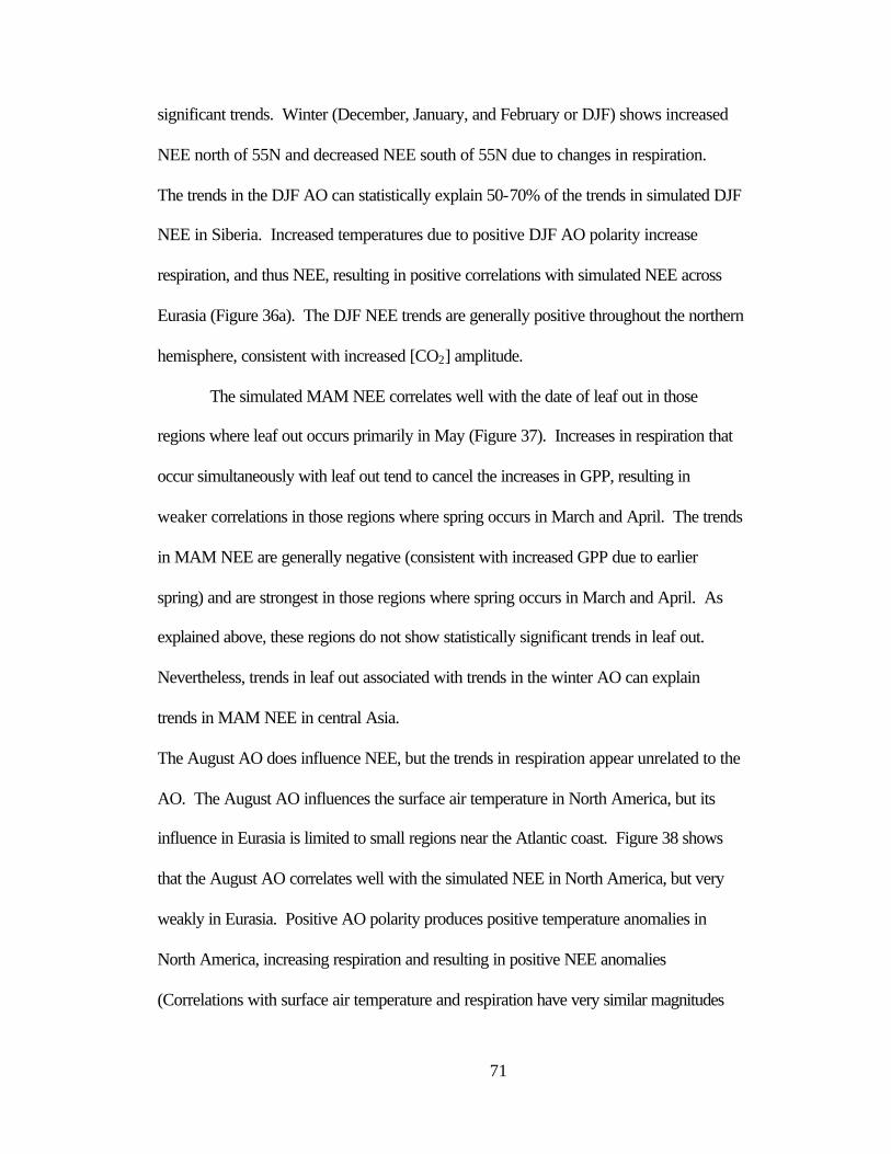
71
significant trends. Winter (December, January, and February or DJF) shows increased
NEE north of 55N and decreased NEE south of 55N due to changes in respiration.
The trends in the DJF AO can statistically explain 50-70% of the trends in simulated DJF
NEE in Siberia. Increased temperatures due to positive DJF AO polarity increase
respiration, and thus NEE, resulting in positive correlations with simulated NEE across
Eurasia (Figure 36a). The DJF NEE trends are generally positive throughout the northern
hemisphere, consistent with increased [CO2] amplitude.
The simulated MAM NEE correlates well with the date of leaf out in those
regions where leaf out occurs primarily in May (Figure 37). Increases in respiration that
occur simultaneously with leaf out tend to cancel the increases in GPP, resulting in
weaker correlations in those regions where spring occurs in March and April. The trends
in MAM NEE are generally negative (consistent with increased GPP due to earlier
spring) and are strongest in those regions where spring occurs in March and April. As
explained above, these regions do not show statistically significant trends in leaf out.
Nevertheless, trends in leaf out associated with trends in the winter AO can explain
trends in MAM NEE in central Asia.
The August AO does influence NEE, but the trends in respiration appear unrelated to the
AO. The August AO influences the surface air temperature in North America, but its
influence in Eurasia is limited to small regions near the Atlantic coast. Figure 38 shows
that the August AO correlates well with the simulated NEE in North America, but very
weakly in Eurasia. Positive AO polarity produces positive temperature anomalies in
North America, increasing respiration and resulting in positive NEE anomalies
(Correlations with surface air temperature and respiration have very similar magnitudes

72
and spatial patterns). As shown in Figure 39, the August AO index has a statistically
significant, positive trend (about 40% of the winter AO trend). However, the temperature
trends, which closely match the NEE trends in Figure 38b, are not consistent with that
expected from a positive trend in the August AO.
Correlations between simulated, zonal total NEE and observed [CO2] amplitudes based
on flask measurements are consistent with the seasonally asymmetric trends in NEE
(Figure 40). While many of the flask sites show trends towards increased seasonal [CO2]
amplitudes, only the Barrow, Alaska site had a sufficiently long enough record (1972-
2002) to pass a statistical significance test. Correlations with DJF total zonal NEE were
not statistically significant, so we could draw no firm conclusion about how the winter
fluxes influence the [CO2] amplitude at Barrow. Negative correlations in MAM zonal
NEE at about 60N latitude indicate that increased GPP in spring (negative NEE
anomalies) increases the [CO2] amplitude at Barrow. Positive correlations with JJA
zonal NEE indicate increased respiration in summer results in increased [CO2] amplitude
at Barrow.
Our results indicate that variability in NEE due to the AO can explain some of the
variability in the [CO2] amplitude. The NEE shows seasonally asymmetric trends
consistent with the observed trend in the [CO2] amplitude. The trends in MAM NEE can
be attributed to the trend towards earlier springs due to the trend in the winter AO. The
trends towards increased DJF NEE result from the winter AO trend, but the flask record
is too short to make a statistically significant link with the [CO2] amplitude trend. The
respiration increases in August contribute to the observed variability and trends in the
[CO2] amplitude, but are not strongly associated with the August AO trend.

73
Our results support the Idso et al., [1999] theory that seasonally asymmetric
fluxes can change the [CO2] seasonal cycle. We found that the timing of maximum and
minimum NEE showed little, if any, inter-annual variation and trends, indicating that the
timing peak photosynthesis did not change and cannot explain the amplitude trends, as
proposed by Chapin et al., [1996] and Stone et al., [2002]. We did not include a transport
model in our simulations, but our analysis indirectly supports the shifting source region
theory proposed by Dargaville et al., [2000] by linking some of the amplitude change to
a trend in winter circulation. The [CO2] seasonal cycle has climate memory because it
integrates the cumulative NEE throughout the year. Consequently, the source region for
the [CO2] seasonal cycle may encompass most of the northern hemisphere, much larger
than the source region for a single flask measurement. Evaluating shifting source regions
requires a detailed analysis of NEE using a transport model.
AO and NDVI
Observed NDVI trends from the FASIR dataset show a consistent spatial pattern all year
round (Figure 41), although the trends in spring (March, April, and May or MAM) are
approximately double the annual average. As seen with the trends in leaf out, the NDVI
trends are statistically significant only in regions of relatively low variability. The winter
AO index correlates with the MAM NDVI in Europe, where the AO has the strongest
influence on temperature and the timing of spring (Figure 42a). Positive AO polarity
results in earlier spring and positive NDVI anomalies. As one might expect, the MAM
NDVI also strongly correlate with the simulated date of spring throughout the northern
hemisphere (Figure 42b). Earlier springs result in positive NDVI anomalies and, thus
negative correlations.

74
Unfortunately, the NDVI time series is not long enough to statistically assess how
much of the NDVI trends result from the trend in the winter AO. The JFM AO does not
have a statistically significant trend over the 17-year time period covered by the FASIR
NDVI (1982-1998). The simulated leaf out shows some statistically significant trends,
but at far fewer points than seen in Figure 29. Without statistically significant trends, we
could not estimate congruent trend fractions with either the JFM AO or the date of leaf
out. Our analysis, therefore, is inconclusive.
5.3 Conclusions
The winter AO directly influences GPP and R through its influence on air
temperature. The soil retains the temperature signal of the winter AO for many months,
influencing respiration fluxes well into spring. By controlling the start of the growing
season, the AO influences the total GPP during spring and early summer, the drawdown
period for [CO2].
Our modeling results indicate that the trend in the winter AO can help explain
observed trends towards earlier leaf out and snowmelt. The modeled leaf out and
snowmelt trends are consistent with observed trends. The trends are also consistent with
the NDVI trends. The AO shows a statistically significant influence on spring trends in
the eastern United States and northern Europe. Increased GPP due to earlier springs
increases the amplitude of the NEE seasonal cycle, partially explaining the increase in
[CO2] amplitude.
We found that the components of the terrestrial biosphere with climate memory
(plant buds, snow pack, and soil temperature) integrate the noisy AO signal over time to
control the transition from winter to spring. In general, positive AO polarity during
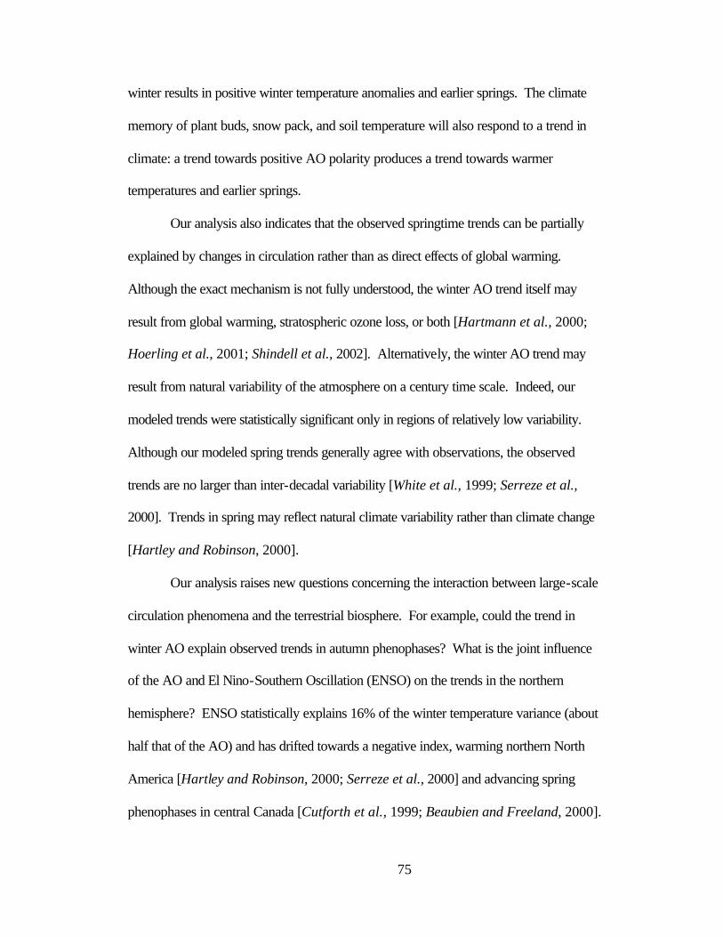
75
winter results in positive winter temperature anomalies and earlier springs. The climate
memory of plant buds, snow pack, and soil temperature will also respond to a trend in
climate: a trend towards positive AO polarity produces a trend towards warmer
temperatures and earlier springs.
Our analysis also indicates that the observed springtime trends can be partially
explained by changes in circulation rather than as direct effects of global warming.
Although the exact mechanism is not fully understood, the winter AO trend itself may
result from global warming, stratospheric ozone loss, or both [Hartmann et al., 2000;
Hoerling et al., 2001; Shindell et al., 2002]. Alternatively, the winter AO trend may
result from natural variability of the atmosphere on a century time scale. Indeed, our
modeled trends were statistically significant only in regions of relatively low variability.
Although our modeled spring trends generally agree with observations, the observed
trends are no larger than inter-decadal variability [White et al., 1999; Serreze et al.,
2000]. Trends in spring may reflect natural climate variability rather than climate change
[Hartley and Robinson, 2000].
Our analysis raises new questions concerning the interaction between large-scale
circulation phenomena and the terrestrial biosphere. For example, could the trend in
winter AO explain observed trends in autumn phenophases? What is the joint influence
of the AO and El Nino-Southern Oscillation (ENSO) on the trends in the northern
hemisphere? ENSO statistically explains 16% of the winter temperature variance (about
half that of the AO) and has drifted towards a negative index, warming northern North
America [Hartley and Robinson, 2000; Serreze et al., 2000] and advancing spring
phenophases in central Canada [Cutforth et al., 1999; Beaubien and Freeland, 2000].

76
ENSO correlates with [CO2] [Braswell et al., 1997] and with NDVI [Los et al., 2001;
Shabanov et al., 2002]. Long simulations such as ours using a highly mechanistic model
driven by reanalysis weather provide an excellent tool for analyzing long-term
interactions between the atmospheric circulation and the terrestrial biosphere.

77
6. Conclusions and Discussion
6.1 Conclusions
Hypothesis 1: the climate influence on NEE has strong regional differences.
We hypothesized that climate influences on NEE inter-annual variability have
strong regional differences. We found that temperature influence on respiration
dominates NEE inter-annual variability in the extra-tropics while precipitation influence
on GPP and R dominates in the tropics. In tropical regions with drier soils, precipitation
control of photosynthesis (i.e., drought stress) dominates. In nearly saturated soils,
precipitation control of respiration dominates. The demarcation between precipitation
control of GPP and R is the line where the average soil moisture is near Wopt, the optimal
soil moisture for respiration.
Hypothesis 2: ENSO influences NEE in the tropics
We hypothesized that ENSO influences NEE in the tropics. We found that the
influence of ENSO on NEE inter-annual variability is consistent with that expected for
shifting precipitation patterns in the tropics. The short time period of our simulation (11
years) precludes any definitive assessment.
Hypothesis 3: the AO influences NEE in the high northern latitudes
We hypothesized that the Arctic Oscillation (AO) influences NEE inter-annual
variability in the high northern latitudes. We found that the AO shows a fairly strong
influence on autumn, winter, and spring NEE through its influence on temperature.
Positive AO polarity indicates positive temperature anomalies, increased respiration, and
thus positive NEE anomalies. The positive temperature anomalies produce positive GPP

78
anomalies and negative NEE anomalies in those regions where spring occurs in March
and April. The influence of the AO on summer NEE is minimal except for North
America in August.
Hypothesis 4: Climate memory allows the winter AO to influence spring NEE
We hypothesized that elements of the land surface have sufficient climate
memory such that the winter AO influences variability in spring and early summer NEE.
The winter AO temperature signal persists for many months in the soil, but its' influence
on respiration drops off by May as the AO temperature anomaly sinks below the soil
carbon. We also found that the winter AO influences the total amount of GPP in spring
and early summer through its influence on the timing of spring. Positive AO polarity
results in earlier springs and greater total GPP.
Hypothesis 5: the winter AO influences variability and trends in the timing of spring
We hypothesized that the winter AO, through its influence on temperature and
precipitation, influences the timing of spring in the northern hemisphere. We found that
those elements of the land system with climate memory (plant buds, snow pack, and soil
temperature) integrate the noisy AO signal over time to control the transition from winter
to spring. The winter AO influences the timing of spring in those regions where the AO
exerts the strongest influence on temperature: Eurasia and southeast United States. Leaf
out, snowmelt, and soil thaw all show the same patterns of influence with the strength of
the correlations increasing with increased climate memory. The winter AO does not
explain variability in the date of spring in the boreal regions of North America.
We hypothesized that the trend in the winter AO are related to observed trends
towards earlier leaf out and snowmelt over large areas in the northern hemisphere. We

79
found that the modeled trends in leaf out, snowmelt, and soil thaw are consistent with
observations. The trends toward earlier spring in southeast United States and Europe
appear statistically related to the trend towards positive AO polarity in winter.
Hypothesis 6: The winter AO influences variability and trends in the [CO2] seasonal amplitude
We hypothesized that winter AO influences inter-annual variability in the [CO2]
seasonal amplitude by simultaneously increasing winter respiration and spring GPP, thus
resulting in a greater [CO2] seasonal amplitude. We found that positive AO polarity
result in positive temperature anomalies that increase the winter buildup of atmospheric
CO2 by increasing respiration and increase spring drawdown by increasing GPP,
particularly in March. We also found that positive AO polarity in winter advances the
start of the growing season, increasing total GPP in spring and early summer and thus the
total atmospheric CO2 drawdown.
We hypothesized that seasonally asymmetric trends in NEE caused by the trend in
the winter AO towards positive polarity is related to the observed trend towards larger
[CO2] seasonal amplitudes. We found that the climate trends in the NCEP reanalysis do
produce seasonally asymmetric trends in NEE. The winter trends towards increased
respiration are consistent with increased temperatures due to the AO. The strong trends
towards increased respiration in August are not related to the August trend towards
positive AO polarity. The trends towards increased GPP in spring are partially explained
by the trends in the winter AO, both directly, through temperature, and indirectly by
advancing the start of the growing season.

80
Hypothesis 7: The winter AO trend is related to NDVI trends
We hypothesized that observed trends towards brighter NDVI is related to the
trend towards positive AO polarity in winter. The NDVI is strongly correlated with the
date of spring. However, Our analysis is inconclusive because the NDVI time record is
too short to estimate statistically significant trends in either the AO or the date of leaf out.
6.2 Discussion
A highly mechanistic model like SiB2 driven by realistic weather is a useful tool
in analyzing the relationship between climate and NEE inter-annual variability. The
process information in SiB2 allows us to understand the exact mechanisms whereby
climate variability influences NEE variability. We can isolate exactly how large-scale
atmospheric phenomena influence NEE.
Climate memory is important in understanding the seasonal dynamics that drive
the global carbon cycle. Those elements of the land system with climate memory (soil,
snow, and plants) control the transition between seasons, and thus the global carbon
cycle. The indirect influence of the AO on NEE variability through climatic memory is
as great or greater than the direct influence through temperature and precipitation.
Climatic memory is a useful paradigm for understanding how climate variability
influences seasonal dynamics of the carbon cycle.
6.3 Future Research
The long simulations created for this research represent a great resource for the
study of NEE variability at a variety of time scales. We focused on how a synoptic scale
phenomenon (the AO) can influence NEE on seasonal and decadal time scales. We

81
answered a small subset of questions concerning the interplay between climate dynamics
and the global carbon cycle. Many other questions remain unanswered or even unasked.
Other Atmospheric Phenomena
Many atmospheric phenomena in addition to the AO and ENSO have strong
regional influences on climate, which would, in turn, influence NEE. Future research
could investigate the relationship between these phenomena and NEE. For example, the
Pacific-North America pattern also influences climate in North American and should be
studied for its effect on NEE. Future research should explain why the Madden-Julian
Oscillation, which influences precipitation and temperatures in the tropics, correlates
strongly with spring NEE in the northern hemisphere. Understanding how these and
other climate phenomena influence NEE provide a strong theoretical basis to explain the
observed variability in the missing carbon sink.
Future research should attempt to explain the strong correlations when NEE lag
the [CO2] growth rate by two years. Similar correlations are observed when the [CO2]
amplitude and NDVI lag temperature by two years [Keeling et al., 1995; Keeling et al.,
1996; Idso et al., 1999; Los et al., 2001].
Seasonal dynamics
Many questions about how climatic memory influences seasonal dynamics remain
unanswered. For instance, the spring variability and trends are not fully explained.
Future research should include an analysis of how ENSO and other atmospheric
phenomena influence the timing of spring in the northern hemisphere, especially in North
America. We have not addressed the transition from autumn to winter. Future research

82
should include an analysis of fall events, which show mixed trends indicating strong
regional differences.
Model Improvements
Our analysis has identified several model improvements that should improve our
estimates of NEE. Using observed leaf out for many more species than just the 15
species of trees and bushes in Europe would improve our estimated date of leaf out.
Incorporating more detailed biogeochemistry would provide better estimates of
respiration. Including the effects of land use change, CO2 fertilization, and nitrogen
deposition would improve the ability of SiB2 to locate and understand the mechanisms
behind the missing carbon sink.
Detailed Comparison with Observations
A logical follow-on study would compare our modeled results directly to
observations. The observations should include snowmelt dates, leaf out dates, soil
temperatures, [CO2] amplitudes, and NEE from flux towers. The reanalysis is optimally
consistent with observations, but nothing beats comparisons with actual data.
Expansion
Future research should expand the scope of our analysis to include other factors
that influence the global carbon cycle. Including a model of ocean fluxes would allow
direct comparison between land and ocean flux variability to test the fundamental
assumption that the ocean fluxes are not as variable as the land fluxes. Adding
atmospheric transport would allow direct comparison between modeled and observed
[CO2] and a more thorough assessment of the [CO2] amplitude trend.

83
7. References
Ahas, R., A. Aasa, A. Menzel, V. G. Fedotova, and H. Scheifinger, Changes in European spring phenology, International Journal of Climatology, 22, 1727-1738, 2002.
Ball, J. T., An analysis of stomatal conductance, Ph.D. Thesis, Stanford University, 1988. Barber, V. A., G. P. Juday, and B. P. Finney, Reduced growth of Alaskan white spruce in the twentieth
century from temperature-induced drought stress, Nature, 405(6787), 668-673, 2000. Beaubien, E. G., and H. J. Freeland, Spring phenology trends in Alberta, Canada: links to ocean
temperature, International Journal of Biometeorology, 44, 53-59, 2000.
Bonan, Gordon B., A Land Surface Model (LSM Version 1.0) for Ecological, Hydrological, and Atmospheric Studies: Technical Description and Users Guide, NCAR Technical Note NCAR/TN-417+STR, Boulder Colorado, 1996.
Bousquet, P, P. Peylin, P. Ciais, C. Le Quéré, P. Friedlingstein, and P.Tans, Regional changes in carbon dioxide fluxes of land and oceans since 1980, Science, 290(5495), 1342-1346, 2000.
Braswell, B. H., D. S. Schimel, E. Linder, and B. Moore, The response of global terrestrial ecosystems to interannual temperature variability, Science, 278(5339), 870-872, 1997.
Cannell, M. G. R. and R. I. Smith, Climatic warming, spring budburst, and frost damage on trees, Journal of Applied Ecology, 23, 177-191, 1986.
Cannell, M. G. R., and R. I. Smith, Thermal time, chill days, and prediction of budburst in picea sitchensis, Journal of Applied Ecology, 20, 951-963, 1983.
Chapin, F. S., S. A. Zimov, G. R. Shaver, and S. E. Hobbie, CO2 fluctuation at high latitudes, Nature, 383(6601), 585-586, 1996.
Chen, X. Q., and W. F. Pan, Relationships among phenological growing season, time-integrated normalized difference vegetation index and climate forcing in the temperate region of eastern China, International Journal of Climatology, 22(14), 1781-1792, 2002.
Chuine, I., A unified model for budburst of trees, Journal of Theoretical Biology, 207, 337-347, 2000. Collatz, G. J., J. T. Ball, C. Grivet, and J. A. Berry, Physiological and Environmental Regulation of
Stomatal Conductance, Photosynthesis, and Transpiration: A Model that Includes a Laminar Boundary Layer, Agricultural and Forest Meteorology, 54, 107-136, 1991.
Collatz, G. J., M. Ribascarbo, and J. A. Berry, Coupled Photosynthesis -Stomatal Conductance Model for Leaves of C4 Plants, Australian Journal of Plant Physiology, 19(5), 519-538, 1992.
Conway, T. J., P. P. Tans, L. S. Waterman, K. W. Thoning, D. R. Kitzis, K. A. Masarie, and N. Zhang, Evidence for Interannual Variability of the Carbon Cycle from the National Oceanic and Atmospheric Administration/Climate Monitoring and Diagnostics Laboratory Global Air Sampling Network, Journal of Geophysical Research, 99(D11), 22,831-22,855, 1994.
Costa, M. H., and J. A. Foley, A Comparison of Precipitation Datasets for the Amazon Basin, Geophysical Research Letters, 25(2), 155-158, 1998.
Craig, S. G., K. J. Holmén, G. B. Bonan, and P. J. Rasch, Atmospheric CO2 simulated by the National Center for Atmospheric Research Community Climate Model. 1. Mean fields and seasonal cycles, Journal of Geophysical Research, 13213-13235, 1998.
Cutforth, H. W., B. G. McConkey, R. J. Woodvine, D. G. Smith, P. G. Jefferson, and O. O. Akinremi, Climate change in the semiarid prairie of southwestern Saskatchewan: Late winter-early spring, Canadian Journal of Plant Science, 79(3), 343-350, 1999.
Dargaville, R. J., R. M. Law, and F. Pribac, Implications of interannual variability in atmospheric circulation on modeled CO2 concentrations and source estimates, Global Biogeochemical Cycles, 14(3), 931-943, 2000.
Defries, R. S. and J. R. G. Townshend, NDVI-derived land cover classification at a global scale, International Journal of Remote Sensing, 15(17), 3567-3586, 1994.

84
Denning, A. S., G. J. Collatz, C. Zhang, D. A. Randall, J. A. Berry, P. J. Sellers, G. D. Colello, and D. A. Dazlich, Simulations of Terrestrial Carbon Metabolism and Atmospheric CO2 in a General Circulation Model Part 1 Surface Carbon Fluxes, Tellus, 48, 521-542, 1996.
Devore, J. L., Probability and Statistics for Engineering and the Sciences, Duxbury Press, 1995. Dickinson, R. E., How coupling of the Atmosphere to ocean and Land Helps Determine the Timescales of
Inter-annual Variability of Climate, Journal of Geophysical Research, 105(D15), 20,115-20,119, 2000.
D'Odorico, P., J. Yoo, and S. Jaeger, Changing seasons: an effect of the North Atlantic Oscillation?, Journal of Climate, 15, 435-445, 2002.
Dye D. G., Variability and trends in the annual snow-cover cycle in Northern Hemisphere land areas, Hydrological Processes, 16(15), 3065-3077, 2002.
Fan, S. M. Gloor, J. Mahlman, S. Pacala, J. Sarmiento, T. Takahashi, and P. Tans, A large terrestrial carbon sink in North America implied by atmospheric and oceanic carbon dioxide data and models, Science, 282(5388), 442-446, 1998.
Farquhar, G. D., S. von Caemmerer, and J. A. Berry, A Biochemical Model of Photosynthetic CO2 Assimilation in Leaves of C3 Species, Planta, 149, 78-90, 1980.
Fung, I., Variable Carbon Sinks, Science, 290, 1313, 2000.
Gibson, J. K., S. Uppala, P. Kållberg, M. Fiorino, A. Hernandez, K. Onogi, and X. Li, ECMWF 40-year Re-Analysis (ERA-40) - Archive Plans, European Centre For Medium-Range Weather Forecasts, 1999.
Goetz, S. J., S. D. Prince, J. Small, and A. C. R. Gleason, Interannual Variability of Global Terrestrial Primary Production: Results of a Model Driven with Satellite Onservations, Journal of Geophysical Research, 105(D15), 20,077-20,091, 2000.
Green, P.M., D. M. Legler, C. J. Miranda V, and J. J. O'Brien, The North American Climate Patterns Associated with El Nino-Southern Oscillation, Center for Ocean-Atmospheric Prediction Studies, Project Report Series 97-1, 1997.
Hartley, S., and D. A. Robinson, A shift in winter season timing in the Northern Plains of the USA as indicated by temporal analysis of heating degree days, International Journal of Climatology, 20(4), 365-379, 2000.
Hartmann, D. L., J. M. Wallace, V. Limpasuvan, D. W. J. Thompson, and J. R. Holton, Can ozone depletion and global warming interact to produce rapid climate change?, Proceeding of the National Academy of Sciences of the United States of America, 97(4), 1412-1417, 2000.
Hicke, J. A., G. P. Asner, J. T. Randerson, C. Tucker, S. Los, R. Birdsey, J. C. Jenkins, C. Field, and E. Holland, Satellite-derived increases in net primary productivity across North America, 1982-1998, Geophysical Research Letters, 29(10), 1427, 2002.
Hicke, J. A., G. P. Asner, J. T. Randerson, C. Tucker, S. Los, R. Birdsey, J. C. Jenkins, and C. Field, Trends in North American net primary productivity derived from satellite observations, 1982-1998, Global Biogeochemical Cycles, 16(2), art. no. 1019, 2002.
Higuchi, K., S. Murayama, and S. Taguchi, Quasi-decadal variation of the atmospheric CO2 seasonal cycle due to atmospheric circulation changes: 1979-1998, Geophysical Research Letters, 29(8), art. no. 1173, 2002.
Hoerling, M. P., J. W. Hurrell, and T. Xu, Tropical origins for recent North Atlantic climate change, Science, 292, 90-92, 2001.
Houghton, R. A., E. A. Davidson, and G. M. Woodwell, Missing sinks, feedbacks, and understanding the role of terrestrial ecosystems in the global carbon balance, Global Biogeochemical Cycles, 12(1), 25-34, 1998.
Houghton, R. A., Interannual variability in the global carbon cycle, Journal of Geophysical Research, 105(D15), 20121-20130, 2000.
Hunt, E. Raymond Jr., Stephen C. Piper, Ramakrishna Nemani, Charles D. Keeling, Ralf D. Otto, and Steven W. Running, Global net carbon exchange and intra-annual atmospheric CO2 concentrations

85
predicted by an ecosystem process model and three-dimensional atmospheric transport model, Global Biogeochemical Cycles, 10(3), 431-456, 1996.
Hunter, A. F., and M. J. Lechowicz, Predicting the timing of budburst in temperate trees, Journal of Applied Ecology, 29(3), 597-604, 1992.
Ichii, K., Y. Matsui, Y. Yamaguchi, and K. Ogawa, Comparison of Global Net Primary Production Trends Obtained From Satellite-Based Normalized Difference Vegetation Index and Carbon Cycle Model, Global Biogeochemical Cycles, 15(2), 351-363, 2001.
Idso, C. D., S. B. Idso, and R. C. Balling, The relationship between near-surface air temperature over land and the annual amplitude of the atmosphere's seasonal CO2 cycle, Environmental and Experimental Botany, 41(1), 31-37, 1999.
Jaagus, J., J. Truu, R. Ahas, and A. Aasa, Spatial and Temporal variability of climatic seasons on the East European Plain in relation to large-scale atmospheric circulation, Climate Research, 23, 111-129, 2003.
Jackson, R. B., J. Canadell, J. R. Ehleringer, H. A. Mooney, O. E. Sala, and E. D. Schulze, A global analysis of root distributions for terrestrial biomes, Oecologia, 108, 389-411, 1996.
Kaduk, J. and M. Heimann, Assessing the Climate Sensitivity of the Global Terrestrial Carbon Cycle Model SILVAN, Physics and Chemistry of the Earth, 1997.
Kaduk, J., and M. Heimann, A prognostic phenology scheme for global terrestrial carbon cycle models, Climate Research, 6(1), 1-19, 1996.
Keeling, C. D., J. F. S. Chin, and T. P. Whorf, Increased activity of northern vegetation inferred from atmospheric CO2 measurements, Nature, 382(6587), 146-149, 1996.
Keeling, C. D., T. P. Whorf, M. Wahlen, and J. Vanderplicht, Interannual extremes in the rate of rise of atmospheric carbon-dioxide since 1980, Nature, 375(6533), 666-670, 1995.
Keyser, A. R., J. S. Kimball, R. R. Nemani, and S. W. Running, Simulating the effects of climate change on the carbon balance of North American high-latitude forests, Global Change Biology, 6, 185-195, 2000.
Kramer, K., Selecting a model to predict the onset of growth of Fagus sylvatica, Journal of Applied Ecology, 31, 172-181, 1994.
Le Quéré, C., J. C. Orr, P. Monfray, O. Aumont, and G. Madec, Interannual variability of the ocean sink of CO2 from 1979 through 1997, Global Biogeochemical Cycles, 14(4), 1247-1265, 2000.
Lloyd, J., Current perspectives on the terrestrial carbon cycle, Tellus Series B: Chemical and Physical Meteorology, 51(2), 336-342, 1999.
Los, S. O., G. J. Collatz, L. Bounoua, P. J. Sellers, and C. J. Tucker, Global Interannual Variations in Sea Surface Temperature and Land-Surface Vegetation, Air Temperature, and Precipitation, Journal of Climate, 14(7), 1535-1549, 2001.
Los, S. O., G. J. Collatz, P. J. Sellers, C. M. Malmstrom, N. H. Pollack, R. S. DeFries, C. J. Tucker, L. Bounoua, M. T. Parris, and D. A. Dazlich, A global 9-year biophysical land surface dataset from NOAA AVHRR data, Journal of Hydrometeorology, 1(2), 183-199, 2000.
Los, S. O., Linkages Between Global Vegetation and Climate: An Analysis Based on NOAA Advanced Very High Resolution Radiometer Data, Goddard Space Flight Center-1998-206852, 1998.
Lucht, W., I. C. Prentice, R. B. Myneni, S. Sitch, P. Friedlingstein, W. Cramer, P. Bousquet, W. Buermann, and B. Smith, Climatic control of the high-latitude vegetation greening trend and Pinatubo effect, Science, 296(5573), 1687-1689, 2002.
McGuire, A. D., S. Sitch, J. S. Clein, R. Dargaville, G. Esser, J. Foley, M. Heimann, F. Foos, J. Kaplin, D. W. Kicklighter, R. A. Meier, J. M. Melillo, B. Moore III, I. C. Prentice, N. Ramankutty, T. Reichenau, A. Schloss, H. Tian, L. J. Williams, and U. Wittenburg, Carbon balance of the terrestrial biosphere in the twentieth century: Analyses of CO2 climate and land use effects with four process-based ecosystem models, Global Biogeochemical Cycles, 15(1), 183-206, 2001.
Menzel, A, and P. Fabian, Growing season extended in Europe, Nature, 397(6721), 659-659, 1999. Menzel, A., Plant phenological anomalies in Germany and their relation to air temperature and NAO,
Climatic Change, 57(3), 243-263, 2003.

86
Menzel, A., Trends in phenological phases in Europe between 1951 and 1996, International Journal of Biometeorology, 44(2), 76-81, 2000.
Murray, M. B., M. G. R. Cannell, and R. I. Smith, Date of budburst of fifteen tree species in Britain following climatic warming, Journal of Applied Ecology, 26, 693-700, 1989.
Myneni, R. B., Keeling, C. D., Tucker, C. J., Asrar, G., and Nemani, R. R., Increased plant growth in the northern high latitudes from 1981 to 1991, Nature, 386(6626), 698-702, 1997.
Nemani, R. M. White, P. Thornton, K. Nishida, S. Reddy, J. Jenkins, and S. Running, Recent trends in hydrologic balance have enhanced the terrestrial carbon sink in the United States, Geophysical Research Letters, 29(10), art. no. 1468, 2002.
Nikolov, N., and K. F. Zeller, Modeing coupled interactions of carbon, water, and ozone exchange between terrestrial ecosystems and the atmosphere I: Model description, Environmental Pollution, 124, 231-246, 2003.
Pacala, S. W., G. C. Hurtt, D. Baker, P. Peylin, R. A. Houghton, R. A. Birdsey, L. Heath, E. T. Sundquist, R. F. Stallard, P. Ciais, P. Moorcroft, J. P. Caspersen, E. Shevliakova, B. Moore, G. Kohlmaier, E. Holland, M. Gloor, M. E. Harmon, S. M. Fan, J. L. Sarmiento, C. L. Goodale, D. Schimel, and C. B. Field, Consistent land-and ocean-based U. S. carbon sink estimates, Science, 292, 2316-2320, 2001.
Parton, W. J., J. M. O. Scurlock, D. S. Ojima, T. G. Gilmanov, R. J. Scholes, D. S. Schimel, T. Kirchner, J-C Menaut, T. Seastedt, E. Garcia Moya, Apinan Kamnalrut, J. I. Kinyamario, Observations and modeling of biomass and soil organic matter dynamics for the grassland biome worldwide, Global Biogeochemical Cycles, 7(4), 785-809, 1993.
Potter, C. S., J. T. Randerson, C. B. Field, P. A. Matson, P. M. Vitousek, H. A. Mooney, and S. A. Klooster, Terrestrial ecosystem production: A process-oriented model based on global satellite and surface data, Global Biogeochemical Cycles, 7, 811-842, 1993.
Potter, C. S., S. Klooster, and V. Brooks, Interannual variability in terrestrial net primary production: Exploration of trends and controls on regional to global scales, Ecosystems, 2(1), 36-48, 1999.
Potter, Christopher S.; Klooster, Steven A., Detecting a terrestrial biosphere sink for carbon dioxide: interannual ecosystem modeling for the mid-1980s, Climatic Change, 42(3), 489-503, 1999.
Prince, S. D., S. N. Goward, S. Goetz, and K. Czajkowski, Interannual Atmosphere-Biosphere Variation: Implications for Observation and Modeling, Journal of Geophysical Research, 105(D15), 20,055-20,063, 2000.
Raich, J. W., and W. H. Schlesinger, The global carbon dioxide flux in soil respiration and its relationship to vegetation and climate, Tellus Series B: Chemical and Physical Meteorology, 44, 81-99, 1992.
Raich, J. W., E. B. Rastetter, J. M. Melillo, D. W. Kicklighter, P. A. Steudler, and B. J. Peterson, Potential Net Primary Prodution in South America: Application of a Global Model, Ecological Applications, 1(4), 399-429, 1991.
Randerson, J. T., Field, C. B., Fung, I. Y., and Tans, P. P., Increases in early season ecosystem uptake explain recent changes in the seasonal cycle of atmospheric CO2 at high northern latitudes, Geophysical Research Letters, 26(17), 2765-2768, 1999.
Randerson, J.T., M.V. Thompson, T.J. Conway, I.Y. Fung, and C.B. Field, The contribution of terrestrial sources and sinks to trends in the seasonal cycle of atmospheric carbon dioxide., Global Biogeochemical Cycles, 11, 535-560, 1997.
Rayner, P. J., and R. M. Law, The interannual variability of the global carbon cycle, Tellus Series B: Chemical and Physical Meteorology, 51(2), 210-212, 1999.
Reichenau, T. G., and G. Esser, Is interannual fluctuations of atmospheric CO2 dominated by combined effect of ENSO and volcanic aerosols, Global Biogeochemical Cycles, 17(4), 1094, doi:10.1029/2002GB002025, 2003.
Robeson, S. M., Increasing growing-season length in Illinois during the 20th century, Climatic Change, 52(1-2), 219-238, 2002.
Sarmiento, J. L., Atmospheric CO2 Stalled, Nature, 356, 697-698, 1993.

87
Schaefer, K., A. S. Denning, N. Suits, J. Kaduk, I. Baker, S. Los, and L. Prihodko, Effect of climate on interannual variability of terrestrial CO2 fluxes, Global Biogeochemical Cycles, 16(4), art. no. 1102, 2002.
Scheifinger, H., A. Menzel, E. Koch, C. Peter, and R. Ahas, Atmospheric mechanisms governing the spatial and temporal variability of phenological phases in central Europe, International Journal of Climatology, 11, 1739-1755, 2002.
Schwartz, M. D., Phenology and springtime surface layer change, Monthly Weather Review, 120, 2570-2578, 1992.
Sellers, P. J., C. J. Tucker, G. J. Collatz, S. O. Los, C. O. Justice, D. A. Dazlich, and D. A. Randall, A global 1° by 1° NDVI data set for climate studies, part II: The generation of global fields of terrestrial biophysical parameters from NDVI, International Journal of Remote Sensing, 15(17), 3519-3545, 1994.
Sellers, P. J., D. A. Randall, G. J. Collatz, J. A. Berry, C. B. Field, D. A. Dazlich, C. Zhang, G. D. Collelo, and L. Bounoua, A Revised Land Surface Parameterization of GCMs, Part I: Model Formulation, Journal of Climate, 9(4), 676-705, 1996.
Sellers, P. J., S. O. Los, C. J. Tucker, C. O. Justice, D. A. Dazlich, G. J. Collatz, and D. A. Randall, A Revised Land Surface Parameterization of GCMs, Part II: The Generation of Global Fields of Terrestrial Biophysical Parameters from Satellite Data, Journal of Climate, 9(4), 706-737, 1996.
Serreze, M. C., J. E. Walsh, F. S. Chapin, T. Osterkamp, M. Dyurgerov, V. Romanovsky, W. C. Oechel, J. Morison, T. Zhang, and R. G. Barry, Observational evidence of recent change in the northern high-latitude environment, Climatic Change, 46(1-2), 159-207, 2000.
Shabanov, N. V., L. M. Zhou, Y. Knyazikhin, R. B. Myneni, and C. J. Tucker, Analysis of interannual changes in northern vegetation activity observed in AVHRR data from 1981 to 1994, IEEE Transactions on Geoscience and Remote Sensing, 40(1), 115-130, 2002.
Shindell, D. T., R. L. Miller, G. A. Schmidt, and L. Pandolfo, Simulation of recent northern winter climate trends by greenhouse-gas forcing, Nature, 399(6735), 452-455, 1999.
Sitch, S., I.C. Prentice, B. Smith, W. Cramer, J. Kaplan, W. Lucht, M. Sykes, K. Thonicke, and S. Venevsky, LPJ - A coupled model of vegetation dynamics and the terrestrial carbon cycle, The role of vegetation dynamics in the control of atmospheric CO2 content, Ph. D. Thesis, 2000.
Slayback, D. A., J. E. Pinzon, S. O. Los, and C. J. Tucker, Northern hemisphere photosynthetic trends 1982-99, Global Change Biology, 9(1), 1-15, 2003.
Stone, R. S., E. G. Dutton, J. M. Harris, and D. Longenecker, Earlier spring snowmelt in northern Alaska as an indicator of climate change, Journal of Geophysical Research: Atmospheres, 107(D10), art. no. 4089, 2002.
Tanja, S., F. Berninger, T. Vesala, T. Markkanen, P. Hari, A. Makela, H. Ilvesniemi, H. Hanninen, E. Nikinmaa, T. Huttula, T. Laurila, M. Aurela, A. Grelle, A. Lindroth, A. Arneth, O. Shibistova, and J. Lloyd, Air temperature triggers the recovery of evergreen boreal forest photosynthesis in spring, Global Change Biology, 9(10), 1410-1426, 2003.
Tans, P. P. and D. W. R. Wallace, Carbon Cycle Research After Kyoto, Tellus Series B: Chemical and Physical Meteorology, 51, 562-571, 1999.
Thompson, D. W. J. and J. M. Wallace, Annular Modes in the Extratropical Circulation. Part I: Month-to-Month Variability, Journal of Climate, 13, 1000-1016, 2000.
Thompson, D. W. J. and J. M. Wallace, Regional Climate Impacts of the Northern Hemisphere Annular Mode, Science, 293, 85-89, 2001.
Thompson, D. W. J., J. M. Wallace, and G. Hegerl, Annular Modes in the Extratropical Circulation. Part II: trends, Journal of Climate, 13, 1018-1036, 2000.
Tian, H. J. M. Melillo, D. W., Kicklighter, A. D. McGuire, J. V. K. Helfrich III, B. Moore, III, and C. J. Vorosmarty, Effect of interannual climate variability on carbon storage in Amazonian ecosystems, Nature, 396, 664-667, 1998.
88
Trolier, M., W. C. White, P. P. Tans, K. A. Masarie, and P. A. Gemery, Monitoring the Isotopic Composition of Atmnospheric CO2: Measurements from the NOAA Global Air Sampling Network, Journal of Geophysical Research, 101(D20), 25,897-25,916, 1996.
Tucker, C. J., D. A. Slayback, J.E. Pinzon, S. O. Los, R. B. Myneni, and M. G. Taylor, Higher northern latitude normalized difference vegetation index and growing season trends from 1982 to 199, International Journal of Biometeorology, 45(4), 184-190, 2001.
Vaganov, E. A., M. K. Hughes, A. V. Kirdyanov, F. H. Schweingruber, and P. P. Silkin, Influence of snowfall and melt timing on tree growth in subarctic Eurasia, Nature, 400(6740), 149-151, 1999.
White, M. A., P. E. Thornton, and S. W. Running, A continental phenology model for monitoring vegetation responses to interannual climatic variability, Global Biogeochemical Cycles, 11(2), 217-234, 1997.
White, M. A., S. W. Running, and P. E. Thornton, The impact of growing season length variability on carbon assimilation and evapotranspiration over 88 years in the eastern US deciduous forest, International Journal of Biometeorology, 42, 139-145, 1999.
Wu, W.L., and A. H. Lynch, Response of the seasonal carbon cycle in high latitudes to climate anomalies, Journal of Geophysical Research: Atmospheres, 105(D18), 22897-22908, 2000.
Zhang, C., D. A. Dazlich, D. A., Randall, P. J. Sellers, A. S. Denning, Calculation of the Global Land Surface Energy, Water, and CO2 Fluxes With an Off-line Version of SiB2, Journal of Geophysical Research, 101(D14), 19061-19075, 1996.
Zhou, L. M., C. J. Tucker, R. K. Kaufmann, D. Slayback, N. V. Shabanov, and R. B. Myneni, Variations in northern vegetation activity inferred from satellite data of vegetation index during 1981 to 1999, Journal of Geophysical Research: Atmospheres, 106(D17), 20,069-20,083, 2001.
Zhou, L., R. K. Kaufmann, Y. Tian, R. B. Myneni, and C. J. Tucker, Relation between interannual variations in satellite measures of northern forest greenness and climate between 1982 and 1999, Journal of Geophysical Research: Atmospheres, 108(D1), art. no. 4004, 2003.
Zimov, S. A., S. P. Davidov, G. M. Zimova, A. I. Davidova, F. S. Chapin, M. C. Chapin, and J. F. Reynolds, Contribution of disturbance to increasing seasonal amplitude of atmospheric CO2, Science, 284(5422), 1973-1976, 1999.
Zimov, S. A., S. P. Davidov, Y. V. Voropaev, S. F. Prosiannikov, I. P. Semiletov, M. G. Chapin, and F. S. Chapin, Siberian CO2 efflux in winter as a CO2 source and cause of seasonality in atmospheric CO2, Climatic Change, 33(1), 111-120, 1996.
Related Documents